Simulation and Performance Evaluation of Parabolic Trough

Simulation and Performance Evaluation of Parabolic Trough Solar Power Plants

by

ANGELA M. PATNODE

A thesis submitted in partial fulfillment of the requirements for the degree of

MASTER OF SCIENCE (MECHANICAL ENGINEERING)

at the

UNIVERSITY OF WISCONSIN-MADISON

2006

Approved by

Professor Sanford A. Klein

January 10, 2006

i

Abstract

Nine Solar Electric Generation Systems (SEGS) built in southern California between 1984

and 1990 continue to produce 14-80 [MWe] of utility-scale electric power each from solar

thermal energy input. The systems collect energy using a synthetic heat transfer fluid

pumped through absorber tubes in the focal line of parabolic trough collectors. The heated

fluid provides the thermal resource to drive a Rankine steam power cycle.

A model for the solar field was developed using the TRNSYS simulation program. The

Rankine power cycle was separately modeled with a simultaneous equation solving software

(EES). The steady-state power cycle performance was regressed in terms of the heat transfer

fluid temperature, heat transfer fluid mass flow rate, and condensing pressure, and

implemented in TRNSYS. TRNSYS component models for the steam condenser and cooling

tower were implemented in the simulation as well. Both the solar field and power cycle

models were validated with measured temperature and flow rate data from the SEGS VI plant

from 1998 and 2005. The combined solar field and power cycle models have been used to

evaluate effects of solar field collector degradation, flow rate control strategies, and

alternative condenser designs on plant performance.

Comparisons of measured solar field outlet temperatures between 1998 and 2005 indicate

some degradation in field performance. The degradation in performance over time may be

attributed, in part, to loss of vacuum in the annulus surrounding the absorber tube. Another

potential contributor to solar field degradation is hydrogen accumulation in the annular

space; hydrogen may dissociate from the synthetic heat transfer fluid and permeate through

ii

the absorber tube into the annulus. The thermal losses and resultant outlet temperatures are

modeled assuming 50% of collectors experience some loss of vacuum and/or hydrogen

permeation. The loss in electric power from the cycle is quantified as a function of the

prevalence of vacuum loss and hydrogen accumulation in the field.

The electric power output from the system at a given incident radiation depends on the

system efficiency, defined as the product of the solar field efficiency and the power cycle

efficiency. The solar field efficiency will decrease with increasing outlet temperature, while

the power cycle efficiency will increase with increasing outlet temperature. The magnitude

of these competing trends is such that the net change in system efficiency with outlet

temperature is small.

The SEGS plants use induced draft cooling towers for heat rejection. Cooling towers provide

an effective means of heat rejection, but require makeup water to compensate for evaporative

losses. The use of air cooled condensers can reduce plant water consumption; however,

system efficiency suffers with the higher condensing pressure. The optimal size of an air

cooled condenser unit is evaluated, and its performance assessed and compared to that of the

current condenser/cooling tower system.

iii

Acknowledgements

I owe thanks first and foremost to my three advisors:

Bill Beckman – Your experience and wisdom have benefited me a great deal. Thank

you for all of your counsel and advice.

Doug Reindl – Thank you for all of your enthusiasm for this project, as well as your

supportive attitude. Maybe some day I’ll learn how to speak in English units.

Sandy Klein – It’s an honor to be your advisee and student. It’s a pleasure to call you

my friend. Thanks for being my rabbit.

I am especially grateful for the feedback and support of all of the Concentrating Solar Power

staff at the National Renewable Energy Laboratory: Hank Price, Nate Blair, Mary Jane Hale,

and Mark Mehos. Special thanks as well to Carin Gummo, Nick Potrovitza, Scott Cawein,

Dan Brake, Harvey Stephens, and all of the SEGS plant personnel that have hosted myself

and other members of the Solar Energy Laboratory for site visits. These trips were an

incredibly valuable part of my research experience, and I am indebted to everyone at SEGS

and NREL that helped make them possible.

To my husband David, for being my sounding board several times: Thanks for letting me

vent my frustrations … and occasionally for solving my problems in doing so.

iv

Thanks to all of the friends and fellow graduate students in the Solar Lab, especially Kate

Edwards, who can always make me smile.

Finally, a special thank you goes to all of my family in Omaha – my parents, Mary and Jerry

Jacobson, and my siblings, Becky, Steve, and Stacy. You are the most important people in

my life.

This research work was sponsored by the National Renewable Energy Laboratory under

Contract 144-MQ55.

v

Table of Contents Abstract ......................................................................................................................................... i

Acknowledgements .................................................................................................................. iii

Table of Contents....................................................................................................................... v

List of Tables.............................................................................................................................. ix

List of Figures ............................................................................................................................ xi

1 Introduction............................................................................................................................. 1

1.1 Background for Solar Electric Generation Systems (SEGS).......................................... 1

1.2 Literature review............................................................................................................. 6

1.3 Objectives of current work.............................................................................................. 8

2 Solar Field Model ................................................................................................................. 11

2.1 Introduction................................................................................................................... 11

2.2 Solar Irradiation Absorption ......................................................................................... 16

2.2.1 Direct Normal Insolation ...................................................................................... 16 2.2.2 Angle of incidence ................................................................................................ 17 2.2.3 Incidence Angle Modifier (IAM).......................................................................... 26 2.2.4 Row Shadowing and End Losses.......................................................................... 28 2.2.5 Field Efficiency and HCE Efficiency ................................................................... 32

2.3 Receiver Heat Loss ....................................................................................................... 34

2.3.1 Analytical Heat Loss Derivation........................................................................... 34 2.3.2 Linear Regression Heat Loss Model..................................................................... 36 2.3.3 Solar Field Piping Heat Losses ............................................................................. 42

2.4 HTF Energy Gain and Temperature Rise ..................................................................... 42

2.5 Heat Transfer Fluid Pumps ........................................................................................... 44

2.6 Model Capabilities and Limitations.............................................................................. 46

3 Power Cycle Model............................................................................................................... 47

3.1 Introduction................................................................................................................... 47

3.2 Temperature – Entropy Diagram .................................................................................. 51

3.3 Assumptions.................................................................................................................. 52

3.4 Component Models....................................................................................................... 54

3.4.1 Superheater / Reheater .......................................................................................... 54 3.4.2 Steam Generator (Boiler)...................................................................................... 62 3.4.3 Preheater ............................................................................................................... 64 3.4.4 Turbine.................................................................................................................. 66 3.4.5 Condenser ............................................................................................................. 70 3.4.6 Pump ..................................................................................................................... 71

vi

3.4.7 Closed Feedwater Heater ...................................................................................... 73 3.4.8 Open Feedwater Heater (Deaerator) ..................................................................... 77 3.4.9 Mixer..................................................................................................................... 79

3.5 Power Generation and Cycle Efficiency....................................................................... 81

3.6 Linear Regression Power Cycle Model ........................................................................ 84

3.7 Conclusions................................................................................................................... 86

4 Balance of System Models.................................................................................................... 88

4.1 Introduction................................................................................................................... 88

4.2 Storage Tank ................................................................................................................. 89

4.3 Water-Cooled Condenser.............................................................................................. 92

4.4 Cooling Tower .............................................................................................................. 95

4.5 Conclusions................................................................................................................... 98

5 Model Validation .................................................................................................................. 99

5.1 Introduction................................................................................................................... 99

5.2 Data Consistency Analysis and Validation................................................................. 102

5.2.1 HTF mass flow rate............................................................................................. 103 5.2.2 HTF inlet temperature......................................................................................... 106 5.2.3 Steam mass flow rate .......................................................................................... 112 5.2.4 Energy Balances.................................................................................................. 114

5.3 Solar Field Model Validation...................................................................................... 117

5.4 Power Cycle Model Validation................................................................................... 132

5.5 Condensing Pressure Predictions versus Plant Data................................................... 145

5.6 System Gross Electric Power Predictions versus Plant Data...................................... 153

5.7 Conclusions................................................................................................................. 161

6 Solar Field Performance Analysis ...................................................................................... 162

6.1 Introduction................................................................................................................. 162

6.2 Assumptions................................................................................................................ 163

6.3 Change in Solar Field Heat Retention and Outlet Temperature ................................. 165

6.4 Effect on Electric Power Output ................................................................................. 172

6.5 Conclusions................................................................................................................. 175

7 Optimized Control of Solar Field Flow Rate...................................................................... 178

7.1 Introduction................................................................................................................. 178

7.2 Solar Field, Power Cycle Efficiency with Flow Rate ................................................. 179

vii

7.3 Impact of Flow Rate Control on Power Output .......................................................... 188

7.4 Conclusions................................................................................................................. 192

8 Alternative Condensers....................................................................................................... 194

8.1 Introduction................................................................................................................. 194

8.2 Air Cooled Condenser Design .................................................................................... 195

8.3 Optimum Size of Air Cooled Condenser for SEGS VI .............................................. 200

8.4 Annual Performance of Condensers ........................................................................... 201

8.5 Simulation Using Air Cooled Condenser ................................................................... 205

8.6 Economics of Dry Condensing ................................................................................... 207

8.7 Conclusions................................................................................................................. 208

9 Conclusions and Recommendations ................................................................................... 210

9.1 Conclusions................................................................................................................. 210

9.2 Recommendations for future work ............................................................................. 212

APPENDICES ............................................................................................................................ 214

viii

ix

List of Tables Table 1.1 Basic Characteristics of SEGS Plants at Kramer Junction ........................................... 2

Table 2.1 Typical optical parameters and correction values for solar field.................................. 34

Table 2.2 Inputs used in HCE heat transfer analysis model ......................................................... 38

Table 2.3 Coefficients for Receiver Heat Loss: Vacuum Annulus.............................................. 38

Table 2.4 Coefficients for Receiver Heat Loss: Air Annulus. .................................................... 38

Table 2.5. Coefficients for Receiver Heat Loss: Hydrogen Annulus. ........................................ 39

Table 3.1. Reference efficiency and pressures for turbine sections............................................. 67

Table 3.2. UAs for closed feedwater heaters ............................................................................... 75

Table 3.3. Coefficients for Equations (3.87) and (3.88) .............................................................. 85

Table 5.1. Plant monitored data used in data consistency analysis and model validation......... 101

Table 5.2. Instrumentation at SEGS VI. .................................................................................... 102

Table 5.3. RMSD through mid-day operation for each simulated day...................................... 131

Table 5.4. Sensitivity of solar field outlet temperature to uncertainty of parameters................ 132

Table 5.5. RMSD and average uncertainty values..................................................................... 143

Table 5.6. Sensitivity analysis for power cycle model as a function of power cycle inputs ..... 144

Table 8.1. Example ACC Parameters and Operating Conditions.............................................. 196

Table 8.2. Design Dry Bulb and Mean Coincident Wet Bulb, Edwards Air Force Base. ......... 202

x

xi

List of Figures

Figure 1.1. Parabolic troughs at a 30 MWe SEGS plant in Kramer Junction, CA........................ 2

Figure 1.2. Solar Collector Assembly (SCA) ................................................................................ 3

Figure 1.3. End of a row of Solar Collector Assemblies (SCAs) .................................................. 4

Figure 1.4. Heat collection element (HCE) ................................................................................... 5

Figure 2.1. Layout of the SEGS VI solar trough field .................................................................. 11

Figure 2.2. Heat collection element (HCE) (not shown to scale) ................................................. 12

Figure 2.3. Schematic of a Solar Collector Assembly (SCA)....................................................... 13

Figure 2.4. Information flow diagram for solar field component ................................................. 14

Figure 2.5. DNI measured at SEGS VI on June 21, 2005, and December 21, 2004. ................... 17

Figure 2.6. Angle of incidence on a parabolic trough collector................................................... 18

Figure 2.7. Declination angle due to Earth's tilt ........................................................................... 19

Figure 2.8. Declination angle variation by month, from Equation (2.2) ...................................... 20

Figure 2.9. Equation of time vs month of the year (from Equation 2.5) ...................................... 22

Figure 2.10. Solar altitude angle versus time, on June 21 and December 21 of the year, for

the SEGS VI location ................................................................................................ 23

Figure 2.11. DNI and DNI cos (θ) at SEGS VI on June 21, 2005............................................... 25

Figure 2.12. DNI and DNI cos (θ) at SEGS VI on December 21, 2004...................................... 25

Figure 2.13. Incidence angle modifier (IAM) versus θ, from Equation (2.11)............................ 28

Figure 2.14. Collector tracking through morning, showing digression of collector shading as

the day progresses ..................................................................................................... 29

Figure 2.15. RowShadow (Weff/W) versus time of day, for June 21 and December 21............... 30

Figure 2.16. End losses from an HCE........................................................................................... 31

Figure 2.17. End Losses versus incidence angle (θ) ..................................................................... 32

Figure 2.18. Heat transfer mechanisms acting on HCE surfaces.................................................. 35

Figure 2.19. Receiver heat loss vs bulk fluid temperature - vacuum annulus at 0.0001[torr] ..... 39

Figure 2.20. Receiver heat loss vs bulk fluid temperature - air in annulus at 760 [torr] ............. 40

Figure 2.21. Receiver heat loss vs bulk fluid temperature - Hydrogen in annulus at 1 [torr] ..... 40

Figure 3.1. Flow diagram for HTF through heat exchangers ...................................................... 48

Figure 3.2. Flow diagram for power cycle - components labeled ............................................... 49

Figure 3.3. Flow diagram for power cycle - state points labeled................................................. 50

xii

Figure 3.4. Temperature-entropy diagram of power cycle at reference state .............................. 52

Figure 3.5. Flow diagram of superheater/reheater ....................................................................... 54

Figure 3.6. Flow diagram of steam generator ............................................................................... 62

Figure 3.7. Flow diagram of preheater.......................................................................................... 64

Figure 3.8. Flow diagram for turbine section .............................................................................. 66

Figure 3.9. Percent reduction in efficiency as a function of throttle flow ratio, for condensing

turbine with one governing stage .............................................................................. 68

Figure 3.10. Flow diagram of condenser ...................................................................................... 70

Figure 3.11. Flow diagram of a pump........................................................................................... 72

Figure 3.12 Flow diagram for a closed feedwater heater............................................................. 74

Figure 3.13. Open feedwater heater diagram................................................................................ 78

Figure 3.14. Flow diagram of mixer ............................................................................................ 80

Figure 3.15. Generator efficiency as a function of load, for a power factor of 1.00 ................... 82

Figure 3.16. Electricity output (gross) vs HTF mass flow, at various HTF temperatures

entering the power cycle............................................................................................ 86

Figure 4.1. Diagram of inputs and outputs for all components in comprehensive model

simulation. ................................................................................................................. 88

Figure 4.2. Information flow diagram for the storage tank.......................................................... 90

Figure 4.3. Information flow diagram for the cooling water condenser. ..................................... 92

Figure 4.4. Information flow diagram for the cooling tower. ...................................................... 96

Figure 5.1. Relative difference associated with heat transfer fluid mass flow rate calculation

for two days in 1998. ............................................................................................... 104

Figure 5.2. Relative difference associated with heat transfer fluid mass flow rate calculation

for two days in 2005. ............................................................................................... 104

Figure 5.3. Difference in measured temperature at the solar field inlet compared to that

determined from mixing of preheater and reheater outlet streams, for two days in

1998. ........................................................................................................................ 108

Figure 5.4. Difference in measured temperature at the solar field inlet as compared to that

predicted from mixing of preheater and reheater outlet streams, for two days in

2005. ........................................................................................................................ 108

xiii

Figure 5.5. Recorded solar field inlet temperature and recorded preheater and reheater HTF

outlet temperatures from September 19, 1998. ....................................................... 110

Figure 5.6. Recorded solar field inlet temperature and recorded preheater and reheater HTF

outlet temperatures from March 12, 2005. .............................................................. 111

Figure 5.7. Relative difference associated with steam mass flow rate measurement for two

days in 1998............................................................................................................. 113

Figure 5.8. Relative difference associated with steam mass flow rate measurements for two

days in 2005............................................................................................................. 113

Figure 5.9. Results of an energy balance over main heat exchanger train for two days in

1998. ....................................................................................................................... 115

Figure 5.10. Results of an energy balance over main heat exchanger train for two days in

2005. ........................................................................................................................ 116

Figure 5.11. Direct normal insolation (DNI) measurements used for 1998 solar field model

validation. ................................................................................................................ 118

Figure 5.12. Direct normal insolation (DNI) measurements for 2005 model validation........... 118

Figure 5.13. Rates of heat absorption and heat loss from the solar field for June 20, 1998...... 120

Figure 5.14. Measured and predicted outlet temperatures from the solar field for June 20,

1998. ........................................................................................................................ 120

Figure 5.15. Rates of heat absorption and heat loss from the solar field for September 19,

1998. ........................................................................................................................ 121

Figure 5.16. Measured and predicted outlet temperatures from the solar field for September

19, 1998. .................................................................................................................. 121

Figure 5.17. Rates of heat absorption and heat loss from the solar field for December 16,

1998. ........................................................................................................................ 122

Figure 5.18. Measured and predicted outlet temperatures from the solar field for December

16, 1998. .................................................................................................................. 122


1998. ........................................................................................................................ 123


14, 1998. .................................................................................................................. 123

Figure 5.21. Rates of heat absorption and heat loss from the solar field for June 11, 2005...... 125

xiv


2005. ........................................................................................................................ 125

Figure 5.23. Rates of heat absorption and heat loss from the solar field for May 20, 2005...... 126

Figure 5.24. Measured and predicted outlet temperatures from the solar field for May 20,

2005. ........................................................................................................................ 126

Figure 5.25. Rates of heat absorption and heat loss from the solar field for April 27, 2005..... 127

Figure 5.26. Measured and predicted outlet temperatures from the solar field for April 27,

2005. ........................................................................................................................ 127

Figure 5.27. Rates of heat absorption and heat loss from the solar field for March 12, 2005... 128

Figure 5.28. Measured and predicted outlet temperatures from the solar field for March 12,

2005. ........................................................................................................................ 128


2004. ....................................................................................................................... 129


12, 2004. .................................................................................................................. 129

Figure 5.31. Gross power predicted by the power cycle model as compared to measured

gross electric power for June 20, 1998................................................................... 133

Figure 5.32. HTF temperature returning to the solar field, predicted by the power cycle

model, as compared to measured solar field inlet temperature, for June 20, 1998. 133

Figure 5.33. Gross power output predicted by the power cycle model as compared to

measured gross electric power for September 19, 1998.......................................... 134

Figure 5.34. HTF temperature returning to the solar field as predicted by the power cycle

model and compared to measured solar field inlet temperature, for September 19,

1998. ........................................................................................................................ 134


measured gross electric power for December 16, 1998. ......................................... 135


model and compared to measured solar field inlet temperature, for December 16,

1998. ........................................................................................................................ 135



xv



1998. ........................................................................................................................ 136


measured gross electric power for June 11, 2005. .................................................. 138

Figure 5.40. HTF temperature returning to solar field predicted by the power cycle model as

compared to measured solar field inlet temperature for June 11, 2005. ................. 138

Figure 5.41 Gross power output predicted by the power cycle model as compared to

measured gross electric power for May 20, 2005. .................................................. 139


model and compared to measured solar field inlet temperature, for May 20, 2005.139


measured gross electric power for April 27, 2005. ................................................. 140


model and compared to measured solar field inlet temperature, for April 27,

2005. ........................................................................................................................ 140


measured gross electric power for March 12, 2005. ............................................... 141


model and compared to measured solar field inlet temperature, for March 12,

2005. ........................................................................................................................ 141





2005. ........................................................................................................................ 142

Figure 5.49. Number of transfer units (NTU) calculated for the cooling tower......................... 148

Figure 5.50. Cooling water temperatures at the inlet and outlet of the steam condenser on

June 20, 1998........................................................................................................... 149

Figure 5.51. Steam condensing pressure on June 20, 1998 ....................................................... 149

xvi


December 16, 1998.................................................................................................. 150

Figure 5.53. Steam condensing pressure on December 16, 1998 .............................................. 150


June 11, 2005........................................................................................................... 151

Figure 5.55. Steam condensing pressure on June 11, 2005 ....................................................... 151


December 12, 2004 ................................................................................................ 152

Figure 5.57. Steam condensing pressure on December 12, 2004 .............................................. 152

Figure 5.58. Gross power output predicted by the comprehensive model as compared to

measured gross electric power on June 20, 1998................................................... 156


measured gross electric power on September 19, 1998......................................... 156


measured gross electric power on December 14, 1998.......................................... 157




measured gross electric power on June 11, 2005................................................... 158


measured gross electric power on May 20, 2005................................................... 158


measured gross electric power on April 27, 2005.................................................. 159


measured gross electric power on March 12, 2005................................................ 159



Figure 6.1. Receiver tube heat loss versus temperature, for various annulus hydrogen

pressures................................................................................................................. 164

Figure 6.2. Rates of heat absorption and heat loss from the solar field for June 11, 2005,

showing predictions for both the vacuum field case and the hydrogen field case. 167

xvii


2005, showing predictions for both the vacuum field case and the hydrogen

field case. ............................................................................................................... 167

Figure 6.4. Rates of heat absorption and heat loss from the solar field for May 20, 2005,

showing predictions for both the vacuum field case and the hydrogen field case..168

Figure 6.5. Measured and predicted outlet temperatures from the solar field for May 20,

2005, showing predictions for both the vacuum field case and the hydrogen field

case......................................................................................................................... 168

Figure 6.6. Rates of heat absorption and heat loss from the solar field for April 27, 2005,

showing predictions for both the vacuum field case and the hydrogen field case. . 169

Figure 6.7. Measured and predicted outlet temperatures from the solar field for April 27,


case. ......................................................................................................................... 169

Figure 6.8. Rates of heat absorption and heat loss from the solar field for March 12, 2005,

showing predictions for both the vacuum field case and the hydrogen field case. . 170

Figure 6.9. Measured and predicted outlet temperatures from the solar field for March 12,


case. ......................................................................................................................... 170

Figure 6.10. Measured and predicted gross electric power for June 11, 2005, showing

predictions for both the vacuum field case and the hydrogen field case................. 172

Figure 6.11. Measured and predicted gross electric power for May 20, 2005, showing


Figure 6.12. Measured and predicted gross electric power for April 27, 2005, showing


Figure 6.13. Measured and predicted gross electric power for March 12, 2005, showing


Figure 7.2. Solar field efficiency versus solar field outlet temperature, at various lines of

constant incident radiation [W/m2]. All lines truncate at a mass flow rate of 500

[kg/s] on the low temperature end and 240 [kg/s] on the high temperature end. .... 181

Figure 7.3. Power cycle efficiency (gross) versus solar field outlet temperature, at various

lines of constant incident radiation.......................................................................... 183

xviii

Figure 7.4. Power cycle efficiency (net) versus solar field outlet temperature, at various lines

of constant incident radiation .................................................................................. 184

Figure 7.5. Gross efficiency of the solar field-power cycle system versus solar field outlet

temperature, at various lines of constant incident radiation. ................................... 186

Figure 7.6. Net efficiency of the solar field-power cycle system versus solar field outlet

temperature, at various lines of constant incident radiation. ................................... 187

Figure 7.7. Solar field mass flow rate, as controlled for various strategies, for May 20, 2005. 189

Figure 7.8. Temperature achieved at solar field outlet, as a result of various flow rate control

strategies, for May 20, 2005.................................................................................... 189

Figure 7.9. Solar field mass flow rate, as controlled for various strategies, for June 11, 2005. 190

Figure 7.10. Temperature achieved at solar field, as a result of various flow rate control

strategies, for June 11, 2005................................................................................. 190

Figure 7.11. Gross and net electric power production predicted as a result of different flow

rate control strategies, for May 20, 2005.............................................................. 191

Figure 7.12. Gross and net electric power production predicted as a result of different flow

rate control strategies, for June 11, 2005.............................................................. 191

Figure 8.1. Condensing pressure and condensing temperature versus number of air cooled

condenser (ACC) units in an array. ...................................................................... 199

Figure 8.2. Gross cycle power, net cycle power with cooling tower, and net cycle power with

air cooled condenser, versus condensing pressure and condensing temperature. 200

Figure 8.3. Condensing pressure obtained in cooling tower and air cooled condenser through

one year. ............................................................................................................... 203

Figure 8.4. Gross power and net power resulting from the cycle for the mean day of each

month of the year.................................................................................................. 204

Figure 8.5. Gross and net power production predicted from measured plant data from June

20, 1998, for both the water cooled cycle (cooling tower) and the air cooled

cycle (ACC).......................................................................................................... 205

1

1 Introduction

1.1 Background for Solar Electric Generating Systems (SEGS)

Nine Solar Electric Generating Systems (SEGS) were built in the Mojave Desert in southern

California between 1984 and 1990. The SEGS plants are concentrating solar power (CSP) plants

which produce electricity using the thermal energy collected from a series of concentrating solar

collectors. This thermal energy drives a conventional Rankine steam power cycle to produce

electricity. The first two SEGS plants (SEGS I and SEGS II) were built in Daggett, CA, between

1984 and 1985, and are rated at 14 [MWe] and 30 [MWe], respectively. A power park of five

SEGS plants (SEGS III through VII), rated at 30 [MWe] each, was then assembled in Kramer

Junction, CA, between 1986 and 1988. The final two SEGS plants (SEGS VIII and IX) are each

rated at 80 [MWe] and were built in Harper Lake, CA, between 1989 and 1990. All nine SEGS

plants were designed, built, and sold by Luz International. The SEGS plants were made

possible, in large part, by substantial investment tax credits at both the state and federal levels, as

well as through the 1978 Federal Public Utility Regulatory Policies Act (PURPA), which

required local utilities to purchase power from qualifying renewable power plants (Price, 1999).

All of the SEGS plants are still in operation today and, collectively, they generate a combined

peak power of 354 [MW]. A portion of the solar field for one 30 MWe SEGS plant is shown in

Figure 1.1.

2

Figure 1.1. Parabolic troughs at a 30 MWe (net) SEGS plant in Kramer Junction, CA

Basic characteristics of the five SEGS plants at the Kramer Junction site are listed in Table 1.1.

Table 1.1 Characteristics of SEGS Plants at Kramer Junction (Source: Cohen et al, 1999)

Plant Startup Year

Capacity (net)

Design Solar Field Supply Temperature

Collector Technology*

Solar Field Size

III 1987 30 MW 349 [C] LS-2 230,300 m2

IV 1987 30 MW 349 [C] LS-2 230,300 m2

V 1988 30 MW 349 [C] LS-2/LS-3 250,560 m2

VI 1988 30 MW 390 [C] LS-2 188,000 m2

VII 1989 30 MW 390 [C] LS-2/LS-3 194,280 m2 *LS-2 and LS-3 are different generations of Luz parabolic collector troughs. The LS-2 model trough is 50 [m] long and has an aperture width of 5 [m]. The LS-3 model is 100 [m] long and has an aperture width of 5.75 [m].

Electric power generation at the SEGS plants begins with the solar field. The solar field is

composed of several rows of single axis tracking collector troughs (Figures 1.2, 1.3). Each

3

trough is formed of float-formed, parabolic-curved mirrors that focus direct radiation from the

sun onto a heat collection element (HCE) that runs through the focal line of each trough. The

concentration ratio of the troughs is 71:1 for the LS-2 collector model and 80:1 for the LS-3

(KJC Operating Company, 2004). The trough axes are oriented due north-south and track the

sun as it traverses the sky from east to west.

Figure 1.2. Solar Collector Assembly (SCA)

4

Figure 1.3. End of a row of Solar Collector Assemblies (SCAs)

The HCE is a steel absorber tube 70 [mm] in diameter, which is coated with either black chrome

or a selective ceramic/metal (cermet) surface coating (Figure 1.4). The absorber tube is

surrounded by a glass envelope; the space between the steel tube and the glass is evacuated to

limit heat losses from the absorber tube to the surrounding environment. The focused radiant

energy from the sun is absorbed through the HCE and transferred to a heat transfer fluid (HTF),

which is a synthetic oil such as a mixture of biphenyl and diphenyl oxide (Therminol VP-1) that

is pumped through each HCE tube (Kearney et al, 1988). The heated HTF is pumped back to the

power plant, where it becomes the thermal resource for steam generation in the power cycle.

5

Figure 1.4. Heat collection element (HCE) (Photo source: Solel UVAC, 2004)

Within the power cycle portion of the plant, the hot HTF is piped through a series of counter-

flow heat exchangers that transfer the thermal energy from the HTF to a feedwater stream to

produce superheated steam. This steam serves as the working fluid in a conventional Rankine

power cycle. Steam is condensed at the bottom of the cycle through a water cooled condenser

and pumped back through a series of feedwater heaters to the cycle’s steam generator. The heat

absorbed by the condenser water is rejected to the environment through an induced draft cooling

tower. The SEGS plants also include an ancillary natural gas fired boiler, which may be used to

supplement solar steam production (up to 25%). The levelized cost of electricity from the SEGS

plants was estimated at $0.14/kWh in 2002 (Price, 2002).

Glass envelope

Vacuum between envelope and absorber

Absorber tube

Heat transfer fluid (HTF) flows through absorber tube

6

1.2 Literature review

Lippke (1995) produced a detailed thermodynamic simulation model of the SEGS VI solar field

and power cycle using EASY simulation software (Lippke, 1995). The objective of this model

was to simulate system behavior during part-load conditions (such as winter months and cloud-

covered days). In this model, design state points from the technical plant description are used to

back-calculate turbine state efficiencies and overall conductance (UA) values for all heat

exchangers in the cycle. The model was validated against hourly plant data for both a clear

summer day and a clear winter day (the year from which data was taken for validation is not

specified).

A team of researchers from Sandia National Laboratories and KJC Operating Company members

designed a simulation model for SEGS VI using TRNSYS (Blair et al, 2001). TRNSYS is a

modular program widely used in the simulation of solar systems and buildings. The aim of the

team was to investigate the potential usefulness of parabolic trough plant modeling in TRNSYS,

as well as to provide modeling capability for the plant over short transient periods in the cycle,

such as during plant start-up and shut-down. Comparison of model predictions to SEGS VI plant

data from a clear day in June and a cloudy day in September of 1991 showed good agreement;

transient effects were shown to be adequately modeled. However, the model was very complex

and ran slowly; convergence problems were also commonly encountered in the model (Price,

personal communication, 2005).

Stuetzle (2002) developed a thermodynamic solar trough model and empirical power plant model

as part of a research initiative focused on solar field control. The aim of this work was to study

the potential gains of linearized predictive (automatic) control of HTF mass flow rate through the

7

solar field to maintain a constant solar field outlet temperature, as opposed to the current

manually operated flow rate control. While the automatic flow rate controller developed in this

study was able to simulate control of the field at a constant solar field outlet temperature, the

study did not find that automatic control of the field yielded significant improvement in gross

power output over what could be achieved by a plant operator (Stuetzle, 2002).

Parabolic trough solar field modeling is under development at the National Renewable Energy

Laboratory (NREL). A parabolic trough solar field model developed by NREL (Price, 2005) is

used as the basis for the solar field model in this study.

A detailed thermodynamic analysis of thermal gains and losses through the heat collection

element was completed by Forristall (2003). This model was validated with several sets of

performance data from the collectors and used to study the influence of difference absorber tube

materials, annulus gases, selective surface coatings, and glass envelope diameters on HCE

performance. The results of this study are implemented in predicting thermal losses from the

solar field for the present investigation.

Other reports have provided background on the SEGS plants in California, particularly efforts to

reduce the cost of energy supplied by these plants. Reducing the Cost of Energy from Parabolic

Trough Solar Power Plants (Price, 2002) summarizes several of the most promising means of

reducing the cost of energy from future SEGS plants, including cost reduction potential due to

solar field size, collector size, thermal storage, and other considerations. The Final Report on the

Operation and Maintenance Improvement Program for Concentrating Solar Power Plants (Cohen

8

et al, 1999) details the results of a six year operations and maintenance improvement study

conducted at the plants.

1.3 Objectives of current work

The SEGS VI solar power plant was chosen for detailed study. A model for the solar field was

developed using the TRNSYS simulation program (TRNSYS, 2005). The Rankine power cycle

was separately modeled with a simultaneous equation solving software (EES, 2005). The

steady-state power cycle performance was regressed in terms of the heat transfer fluid

temperature, heat transfer fluid mass flow rate, and condensing pressure, and implemented in

TRNSYS. TRNSYS component models for the steam condenser and cooling tower were

implemented in the simulation as well. Both the solar field and power cycle models were

validated with measured temperature and flow rate data from the SEGS VI plant from 1998 and

2005. The combined solar field and power cycle models have been used to evaluate effects of

solar field collector degradation, HTF flow rate control strategies, and alternative condenser

designs on overall plant performance.

Chapter 2 reviews modeling of the solar field. Power cycle modeling is discussed in Chapter 3.

Models of the thermal capacitance tank, cooling water condenser, and cooling tower are

summarized in Chapter 4. Chapter 5 discusses both solar field and power cycle validation with

plant measurements. Comparisons of measured solar field outlet temperatures between 1998 and

2005 seem to indicate that some degradation in field performance has occurred. In Chapter 6,

the combined solar field – power cycle model is used to quantify performance degradation of the

9

solar field in the period between 1998 and 2005, due to loss of vacuum in the annulus space and

hydrogen permeation through the annulus into the absorber space. Chapter 7 contains an

analysis of solar field flow rate control, including the effects of solar field flow rate on solar field

efficiency, power cycle efficiency, and overall system efficiency. Solar field efficiency

decreases with increasing temperature, while the opposite trend is seen in the power cycle; the

magnitude of these competing efficiency trends is such that the net change in system efficiency

with outlet temperature is small. Chapter 8 reviews the design and performance of an air cooled

condenser in place of the current cooling water condenser and cooling tower system. The use of

air cooled condensers can reduce plant water consumption; however, system efficiency suffers

with the higher condensing pressure. Conclusions and recommendations resulting from this

work are summarized in Chapter 9.

10

11

2 Solar Field Model

2.1 Introduction

The layout of the SEGS VI solar field is shown in Figure 2.1.

Figure 2.1. Layout of the SEGS VI solar trough field. The superimposed arrows indicate the direction of heat

transfer fluid flow. (Photo source: KJC Operating Company, 2005)

Heat transfer fluid (HTF) is pumped from the steam heat exchangers in the power cycle to the

east and west solar fields through the east and west supply headers. The supply headers

distribute the HTF through 50 parallel loops of solar collectors. Each collector loop consists of

Power Block

East Field West Field

Return Headers

Supply Headers Headers

12

16 solar collector assemblies (SCAs), arranged in two parallel rows of 8 SCAs each. The HTF

travels away from the supply (cold) header through one row of the collector loop and back

toward the return (hot) header through the other row. The hot HTF from the collector loops then

merges in the return headers and is pumped back to the central power plant.

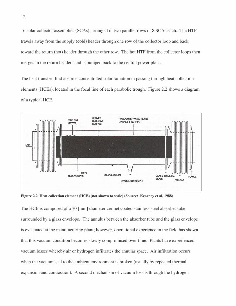
The heat transfer fluid absorbs concentrated solar radiation in passing through heat collection

elements (HCEs), located in the focal line of each parabolic trough. Figure 2.2 shows a diagram

of a typical HCE.

Figure 2.2. Heat collection element (HCE) (not shown to scale) (Source: Kearney et al, 1988)

The HCE is composed of a 70 [mm] diameter cermet coated stainless steel absorber tube

surrounded by a glass envelope. The annulus between the absorber tube and the glass envelope

is evacuated at the manufacturing plant; however, operational experience in the field has shown

that this vacuum condition becomes slowly compromised over time. Plants have experienced

vacuum losses whereby air or hydrogen infiltrates the annular space. Air infiltration occurs

when the vacuum seal to the ambient environment is broken (usually by repeated thermal

expansion and contraction). A second mechanism of vacuum loss is through the hydrogen

13

infiltrating the annual space. In this case, free hydrogen is generated by the heat transfer fluid

dissociating slowly over time. Hydrogen then permeates through the stainless steel absorber tube

and accumulates in the annular space. The impact of both air and hydrogen infiltration on the

thermal losses from the field is discussed further in Chapter 6. The metal bellows at either end

of the tube compensates for thermal expansion differences between the absorber material and the

envelope material. Convection and radiation losses to the ambient air occur from the outermost

surface of the HCE.

A schematic of the entire solar collector assembly (SCA), which shows the support structure and

location of drive controls for the system, is shown in Figure 2.3.

Figure 2.3. Schematic of a Solar Collector Assembly (SCA) (Source: Stuetzle, 2002)

The gross HTF temperature rise across the solar field during peak summer periods is on the order

of 100 [°C], from a cold inlet temperature of 293 [°C] to a hot outlet temperature around 390

Heat Collection Element

Mirror

Mirror

Hydraulic Drive System with Controller

Drive Pylon

Intermediate Pylon

Connections, Arms,

14

[°C] at the SEGS VI field. During cloudy days and off-summer periods, the temperature rise

will be lower for a constant flow rate. The actual temperature achieved at the solar field outlet

depends on a number of variables, including the following: HTF flow rate, solar field inlet

temperature, incident solar radiation, thermal losses, cleanliness of the collectors, tracking

precision, and surface properties of the collector field materials.

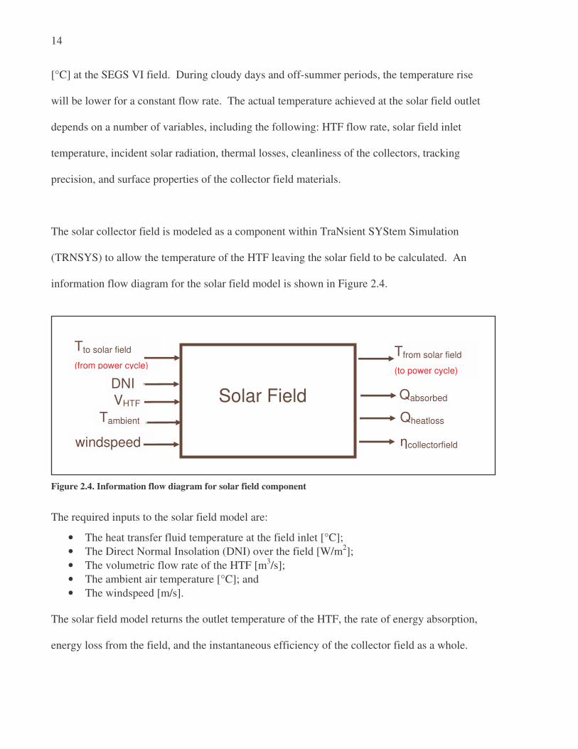
The solar collector field is modeled as a component within TraNsient SYStem Simulation

(TRNSYS) to allow the temperature of the HTF leaving the solar field to be calculated. An

information flow diagram for the solar field model is shown in Figure 2.4.

Figure 2.4. Information flow diagram for solar field component

The required inputs to the solar field model are:

• The heat transfer fluid temperature at the field inlet [°C];

• The Direct Normal Insolation (DNI) over the field [W/m2];

• The volumetric flow rate of the HTF [m3/s];

• The ambient air temperature [°C]; and

• The windspeed [m/s]. The solar field model returns the outlet temperature of the HTF, the rate of energy absorption,

energy loss from the field, and the instantaneous efficiency of the collector field as a whole.

Tfrom solar field

(to power cycle)

Tto solar field

(from power cycle)

DNI

VHTF

windspeed

Solar Field Tambient

Qabsorbed

Qheatloss

ηcollectorfield

15

The procedure for calculating the solar field outlet temperature can be divided into three parts.

First, the absorbed radiation, absorbedQ� , is calculated; absorbedQ� is defined as the energy from the

sun that is actually absorbed by the heat transfer fluid through the absorber tube. The absorbed

radiation will be some fraction of the direct normal insolation, adjusted for incidence angle, row

shading, solar field availability, collector cleanliness, and the collector field and HCE surface

properties. Next, the heat loss from the receivers, heatlossQ� , is calculated. Heat loss from the

receivers will occur due to convection and radiation between the outermost HCE surface and the

ambient air. Thermal losses from the piping leading to and from the collector loops are included

in the heatlossQ� term as well. A simple energy balance shows that the difference between the

absorbed radiation and the receiver heat loss is the effective energy gain of the HTF, collectedQ� .

Knowing the useful energy gain to the HTF and the entering fluid enthalpy allows determination

of the HTF leaving enthalpy. The outlet temperature of the HTF can then be determined from

the field outlet enthalpy.

Calculations of absorbed solar radiation, receiver heat loss, and solar field outlet temperature are

described in further detail in the following sections.

16

2.2 Solar Irradiation Absorption

The equation for the absorbed solar radiation is:

cos( )absorbed field HCE

Q DNI IAM RowShadow EndLoss SFAvailθ η η= ⋅ ⋅ ⋅ ⋅ ⋅ ⋅ ⋅� (2.1)

where

absorbedQ� = solar radiation absorbed by the receiver tubes [W/m2]

DNI = direct normal insolation [W/m2]

θ = angle of incidence [deg]

IAM = incidence angle modifier [-]

RowShadow = performance factor that accounts for mutual shading of parallel collector rows during early morning and late evening [-]

EndLoss = performance factor that accounts for losses from ends of HCEs [-]

ηfield = field efficiency that accounts for losses due to mirror optics and imperfections [-]

ηHCE = HCE efficiency that accounts for losses due to HCE optics and imperfections [-]

SFAvail = fraction of the solar field that is operable and tracking the sun [-]

Each parameter in Equation (2.1) is discussed in further detail in the following sections. 2.2.1 Direct Normal Insolation Extraterrestrial solar radiation follows a direct line from the sun to the Earth. Upon entering the

earth’s atmosphere, some solar radiation is diffused by air, water molecules, and dust within the

atmosphere (Duffie and Beckman, 1991). The direct normal insolation represents that portion of

solar radiation reaching the surface of the Earth that has not been scattered or absorbed by the

atmosphere. The adjective “normal” refers to the direct radiation as measured on a plane normal

to its direction.

17

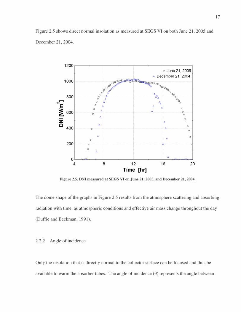
Figure 2.5 shows direct normal insolation as measured at SEGS VI on both June 21, 2005 and

December 21, 2004.

Figure 2.5. DNI measured at SEGS VI on June 21, 2005, and December 21, 2004.

The dome shape of the graphs in Figure 2.5 results from the atmosphere scattering and absorbing

radiation with time, as atmospheric conditions and effective air mass change throughout the day

(Duffie and Beckman, 1991).

2.2.2 Angle of incidence

Only the insolation that is directly normal to the collector surface can be focused and thus be

available to warm the absorber tubes. The angle of incidence (θ) represents the angle between

18

the beam radiation on a surface and the plane normal to that surface. The angle of incidence will

vary over the course of the day (as well as throughout the year) and will heavily influence the

performance of the collectors.

Figure 2.6 illustrates the angle of incidence between the collector normal and the beam radiation

on a parabolic trough. The angle of incidence results from the relationship between the sun’s

position in the sky and the orientation of the collectors for a given location.

Figure 2.6. Angle of incidence on a parabolic trough collector

The position of the sun varies throughout the year. The declination angle is the angular position

of the sun at solar noon, with respect to the plane of the equator. If the earth rotated upright on

its axis, there would be no change in declination angle as the earth revolved around the sun.

Sun

Tracking rotation

Tracking axis

Plane of collector aperture

Line normal to collector aperture

Beam radiation

θ

19

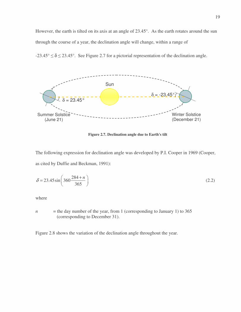
However, the earth is tilted on its axis at an angle of 23.45°. As the earth rotates around the sun

through the course of a year, the declination angle will change, within a range of

-23.45° ≤ δ ≤ 23.45°. See Figure 2.7 for a pictorial representation of the declination angle.

Figure 2.7. Declination angle due to Earth's tilt

The following expression for declination angle was developed by P.I. Cooper in 1969 (Cooper,

as cited by Duffie and Beckman, 1991):

28423.45sin 360

365

nδ

+ =

(2.2)

where

n = the day number of the year, from 1 (corresponding to January 1) to 365 (corresponding to December 31).

Figure 2.8 shows the variation of the declination angle throughout the year.

Sun

Summer Solstice (June 21)

Winter Solstice (December 21)

δ = 23.45° δ = -23.45°

20

Figure 2.8. Declination angle variation by month, from Equation (2.2)

The position of the sun depends on the hour angle, or the angular displacement of the sun east or

west of the local meridian. The hour angle is negative when the sun is east of the local meridian

(in the morning), positive when the sun is west of the local meridian (afternoon), and zero when

the sun is in line with the local meridian (noon).

The hour angle comes as a result of the rotation on the earth, which spins on its axis at a rate of

15° per hour:

( 12) 15hr

SolarTimeω °= − ⋅ (2.3)

where ω is the hour angle [deg] and SolarTime is the solar time [hr].

21

There is an important distinction between standard time and solar time. In solar time, the sun

aligns with the local meridian (ω = 0) at exactly 12:00, or “solar noon.” However, standard time

is based not on the local meridian, but on a standard meridian for the local time zone. The length

of the solar day also varies; this variation is due primarily to the fact that the earth follows an

elliptical path around the sun (Stine and Harrigan, 1985). As a result, the standard time must be

adjusted to reflect the current time of day in solar time. The relationship between solar time and

standard time, in hours, is:

1

60 min

( )

15st loc hL L

SolarTime StandardTime DST E−

= − + + ⋅ (2.4)

where

DST = Daylight Savings Time adjustment (1 [hr] during Daylight Savings Time, 0 [hr] during standard time)

Lst = standard meridian for the local time zone [deg]

Lloc = the local meridian of the collector site [deg]

E = equation of time [min]

E, the equation of time, accounts for the small irregularities in day length that occur due to the

Earth’s elliptical path around the sun. The equation of time used here, in minutes, comes from

Spencer (as cited by Iqbal, 1983):

229.18(0.000075 0.001868cos( ) 0.032077sin( )

0.014615cos(2 ) 0.04089sin(2 ))

E B B

B B

= + −

− − (2.5)

where

360( 1)

365B n= − [deg] (2.6)

n = day number of the year (1 for January 1, 365 for December 31)

22

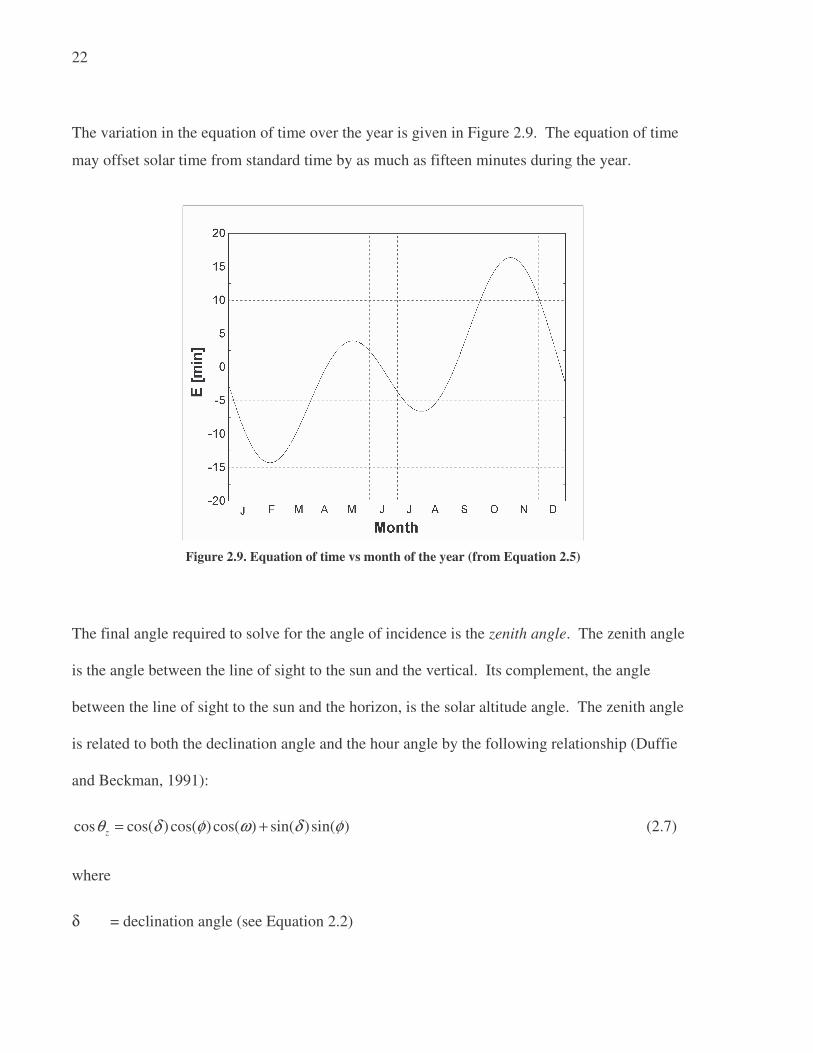
The variation in the equation of time over the year is given in Figure 2.9. The equation of time

may offset solar time from standard time by as much as fifteen minutes during the year.

Figure 2.9. Equation of time vs month of the year (from Equation 2.5)

The final angle required to solve for the angle of incidence is the zenith angle. The zenith angle

is the angle between the line of sight to the sun and the vertical. Its complement, the angle

between the line of sight to the sun and the horizon, is the solar altitude angle. The zenith angle

is related to both the declination angle and the hour angle by the following relationship (Duffie

and Beckman, 1991):

cos cos( ) cos( ) cos( ) sin( )sin( )zθ δ φ ω δ φ= + (2.7)

where

δ = declination angle (see Equation 2.2)

23

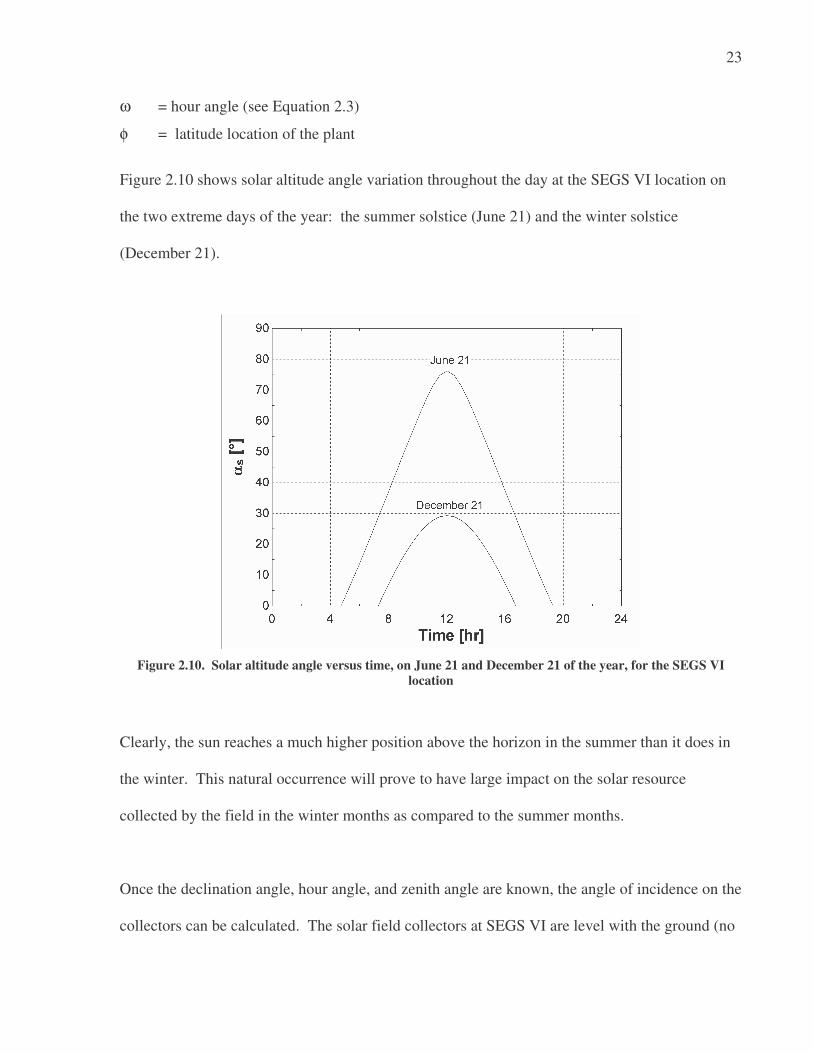
ω = hour angle (see Equation 2.3)

φ = latitude location of the plant

Figure 2.10 shows solar altitude angle variation throughout the day at the SEGS VI location on

the two extreme days of the year: the summer solstice (June 21) and the winter solstice

(December 21).

Figure 2.10. Solar altitude angle versus time, on June 21 and December 21 of the year, for the SEGS VI

location

Clearly, the sun reaches a much higher position above the horizon in the summer than it does in

the winter. This natural occurrence will prove to have large impact on the solar resource

collected by the field in the winter months as compared to the summer months.

Once the declination angle, hour angle, and zenith angle are known, the angle of incidence on the

collectors can be calculated. The solar field collectors at SEGS VI are level with the ground (no

24

vertical tilt) and are oriented due north-south. With a single-axis tracking system, the collectors

are capable of tracking the sun from a position 10° above the eastern horizon to 10° above the

western horizon. In the model, the assumption is made that the collectors are tracking during all

times the sun is above the horizon.

The incidence angle for a plane rotated about a horizontal north-south axis with continuous east-

west tracking to minimize the angle of incidence is given by (Duffie and Beckman, 1991):

2 2 2cos cos cos sinz

θ θ δ ω= + (2.8)

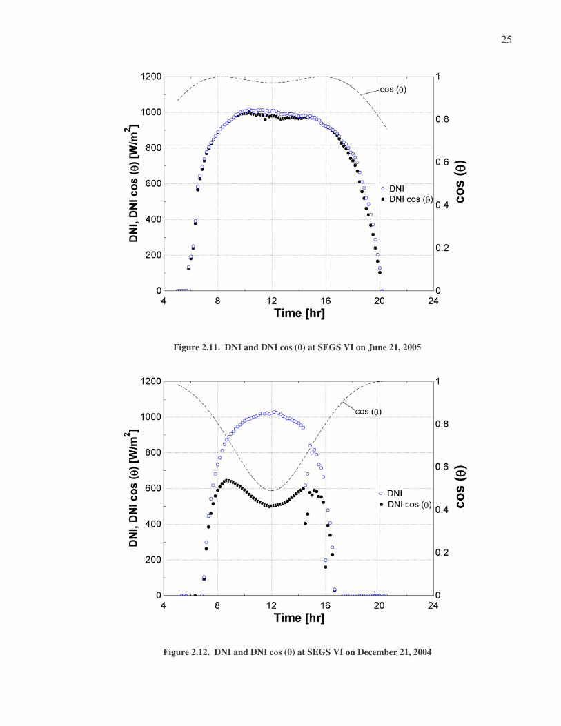
Figures 2.11 and 2.12 show variation of (DNI cos(θ)) throughout the day, as calculated for the

SEGS VI collector location, orientation, and tracking capability. For reference, the direct normal

insolation and cosine of the incidence angle are shown on the graphs as well. The summer

solstice (June 21, 2005) is shown in Figure 2.11; the winter solstice (December 21, 2004) is

shown in Figure 2.12.

25

Figure 2.11. DNI and DNI cos (θ) at SEGS VI on June 21, 2005

Figure 2.12. DNI and DNI cos (θ) at SEGS VI on December 21, 2004

26

The impact of the lower solar altitude angle in the winter is clearly seen in comparing Figure

2.11 to Figure 2.12. There is also a noticeable sag in DNI cos(θ) around noon in Figure 2.12.

The sun rises above the southeast horizon and sets beneath the southwest horizon. With a fixed

north-south orientation and east-west single-axis tracking system, the incidence angle is much

larger at noon in December than it is during morning or afternoon hours, which results in the

shape of the plot seen in Figure 2.12. Over the course of an entire year, the north-south oriented

single-axis tracking receives slightly more energy than an east-west single-axis tracking aperture

in the same location (Stine and Harrigan, 1984). Also, the north-south oriented tracking aperture

receives more energy in the summertime, when electricity demand is highest and the solar

collectors are designed for their peak performance.

2.2.3 Incidence Angle Modifier (IAM)

In addition to losses due to the angle of incidence, there are other losses from the collectors that

can be correlated to the angle of incidence. These losses occur due to additional reflection and

absorption by the glass envelope when the angle of incidence increases. The incidence angle

modifier (IAM) corrects for these additional reflection and absorption losses. The incidence

angle modifier is given as an empirical fit to experimental data for a given collector type.

The solar collector assemblies at the SEGS VI plant are Luz Solar collectors, second generation

(LS-2). Based on performance tests conducted at Sandia National Laboratories on an LS-2

collector, the incidence angle modifier for the collector is (Dudley, 1994):

2cos( ) 0.000884( ) 0.00005369( )K θ θ θ= + − (2.9)

27

where θ, the incidence angle, is provided in degrees.

It is desirable to distinguish between losses in available radiation due to the angle of incidence

itself and the reflection/absorption corrections empirically correlated to the angle of incidence.

For this purpose, the incidence angle modifier is defined for this work as the incidence angle

modifier defined by Dudley et al, divided by the cosine of the incidence angle:

cos( )

KIAM

θ= (2.10)

The equation for the incidence angle modifier used in the solar field component model is:

2

1 0.000884 0.00005369cos( ) cos( )

IAMθ θ

θ θ= + ⋅ − ⋅ (2.11)

The variation of the incidence angle modifier (IAM) is shown versus the incidence angle (θ) in

Figure 2.13. The cosine of the incidence angle is provided in Figure 2.13 for reference.

28

Figure 2.13. Incidence angle modifier (IAM) versus θ, from Equation (2.11)

2.2.4 Row Shadowing and End Losses

The positioning and geometry of the collector troughs and HCEs can introduce further losses,

due to shading of parallel rows in the morning and evening as well as end losses from the HCE.

The following discussion of collector shading is based on Stuetzle (2002). At SEGS VI, the

collectors are arranged in parallel rows, with about 15 [m] of spacing between each row. In the

early morning, all of the collectors face due east. Due to the low solar altitude angle of the sun in

the morning, the eastern-most row of collectors will receive full sun, but this row will shade all

subsequent rows to the west. As the sun rises and the collectors track the sun, this mutual row

shading effect decreases, until a critical zenith angle is reached at which no row shading occurs.

Collector rows remain un-shaded through the middle of the day, from late morning through early

29

afternoon. Mutual row shading then re-appears in the late afternoon and evening, when the solar

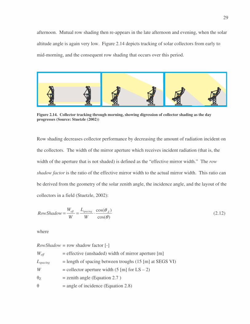
altitude angle is again very low. Figure 2.14 depicts tracking of solar collectors from early to

mid-morning, and the consequent row shading that occurs over this period.

Figure 2.14. Collector tracking through morning, showing digression of collector shading as the day

progresses (Source: Stuetzle (2002))

Row shading decreases collector performance by decreasing the amount of radiation incident on

the collectors. The width of the mirror aperture which receives incident radiation (that is, the

width of the aperture that is not shaded) is defined as the “effective mirror width.” The row

shadow factor is the ratio of the effective mirror width to the actual mirror width. This ratio can

be derived from the geometry of the solar zenith angle, the incidence angle, and the layout of the

collectors in a field (Stuetzle, 2002):

cos( )

cos( )

eff spacing ZW L

RowShadowW W

θ

θ= = ⋅ (2.12)

where

RowShadow = row shadow factor [-]

Weff = effective (unshaded) width of mirror aperture [m]

Lspacing = length of spacing between troughs (15 [m] at SEGS VI)

W = collector aperture width (5 [m] for LS – 2)

θZ = zenith angle (Equation 2.7 )

θ = angle of incidence (Equation 2.8)

30

Equation 2.12 is bounded with a minimum value of 0 (rows are fully shaded) and a maximum

value of 1 (rows are not shaded). Figure 2.15 shows variation of the row shadow factor through

the day, both for the summer solstice and the winter solstice. As seen in Figure 2.15, losses are

introduced by collector shading during approximately the first and last 90 minutes of operation

each day. Because the collectors are single-axis tracking in a north-south orientation, the length

of time over which row shading occurs does not vary significantly throughout the year.

Figure 2.15. RowShadow (Weff/W) versus time of day, for June 21 and December 21

End losses occur at the ends of the HCEs, where, for a nonzero incidence angle, some length of

the absorber tube is not illuminated by solar radiation reflected from the mirrors. Figure 2.16

depicts the occurrence of end losses for an HCE with a nonzero angle of incidence.

31

Figure 2.16. End losses from an HCE

The end losses are a function of the focal length of the collector, the length of the collector, and

the incident angle (Lippke, 1995):

tan( )1

SCA

fEndLoss

L

θ= − (2.13)

where

f = focal length of the collectors (5 [m] at SEGS VI)

θ = incident angle (see Equation 2.8)

LSCA = length of a single solar collector assembly (50 [m] at SEGS VI)

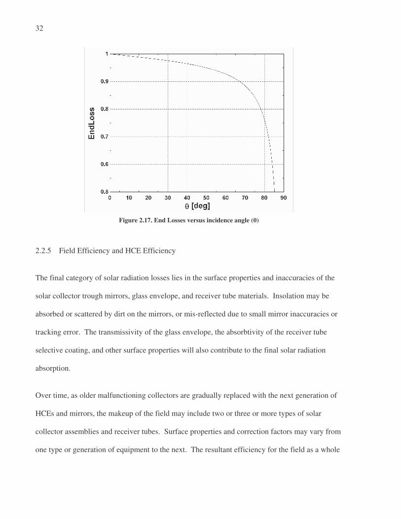
Figure 2.17 shows variation of end losses with incidence angle.

Beam radiation

f

θ

End loss

32

Figure 2.17. End Losses versus incidence angle (θ)

2.2.5 Field Efficiency and HCE Efficiency The final category of solar radiation losses lies in the surface properties and inaccuracies of the

solar collector trough mirrors, glass envelope, and receiver tube materials. Insolation may be

absorbed or scattered by dirt on the mirrors, or mis-reflected due to small mirror inaccuracies or

tracking error. The transmissivity of the glass envelope, the absorbtivity of the receiver tube

selective coating, and other surface properties will also contribute to the final solar radiation

absorption.

Over time, as older malfunctioning collectors are gradually replaced with the next generation of

HCEs and mirrors, the makeup of the field may include two or three or more types of solar

collector assemblies and receiver tubes. Surface properties and correction factors may vary from

one type or generation of equipment to the next. The resultant efficiency for the field as a whole

33

is assumed in the model to be the weighted average of the performance of each type of

component found in the field.

The sum effect of surface and correction parameters for the collector assembly and mirrors is

accounted for in the field efficiency term, ηfield :

1

NumCol

field i i i i i

i

ColFrac TrkTwstErr GeoAcc MirRef MirClnη=

= ⋅ ⋅ ⋅ ⋅∑ (2.14)

where NumCol = the number of collector types in the field

ColFrac = the fraction of collector type in the field

TrkTwstErr = twisting and tracking error associated with the collector type

GeoAcc = geometric accuracy of the collector mirrors

MirRef = mirror reflectivity

MirCln = mirror cleanliness

The sum effect of surface and correction parameters for the heat collection element is accounted

for in the HCE efficiency term, ηHCE :

1

NumHCE

HCE i i i i i i

i

HCEFrac HCEdust BelShad EnvTrans HCEabs HCEmiscη=

= ⋅ ⋅ ⋅ ⋅ ⋅∑ (2.15)

where NumHCE = the number of HCE types in the field

HCEFrac = the fraction of HCE type in the field

HCEdust = losses due to shading of HCE by dust on the envelope

BelShad = losses from shading of ends of HCEs due to bellows

EnvTrans = transmissivity of the glass envelope

HCEabs = absorbtivity of the HCE selective coating

HCEmisc = miscellaneous factor to adjust for other HCE losses

34

Typical surface properties and correction parameters for the collector field and HCE are shown

in Table 2.1.

Table 2.1 Typical optical parameters and correction values for solar field

(Source: Price, 2005, and Forristall, 2003)

Name Value Name Value

TrkTwstErr 0.99 HCEdust 0.98

GeoAcc 0.98 BelShad 0.97

MirRef 0.93 EnvTrans 0.96

MirCln 0.95 HCEabs 0.95

HCEmisc 0.96

For SEGS VI, using the parameters listed in Table 2.1, the field efficiency calculated is 0.857,

and the HCE efficiency calculated is 0.832. Together, the incident radiation losses due to surface

properties and focusing and cleanliness correction factors are 0.7133.

2.3 Receiver Heat Loss

As the heat transfer fluid in the receiver tubes absorbs energy, its temperature will increase. This

temperature increase creates a temperature difference between the bulk temperature of the fluid

and the temperature of the surrounding ambient air. Heat losses from the receiver tube to the

glass envelope, as well as from the glass envelope to the ambient air, are driven by this

temperature difference. This parasitic heat loss can be correlated with the temperature of the

heat transfer fluid, as described further below.

2.3.1 Analytical Heat Loss Derivation

Figure 2.18 shows the relevant heat transfer mechanisms responsible for losses between the

collector surfaces and the ambient environment.

35

Figure 2.18. Heat transfer mechanisms acting on HCE surfaces

The heat fluxes into each surface of the HCE must balance the fluxes leaving that surface. For a

given bulk fluid temperature, insolation, ambient weather conditions, HCE dimensions, and HCE

surface properties, energy balances over each surface of the HCE can be used to determine

surface temperatures, the net heat flux absorbed by the fluid, and the net heat flux lost to the

surroundings. Heat transfer analysis of the HCEs using simultaneous equation solving of these

heat transfer rates was accomplished by Forristall (2003). The program developed by Forristall

is used to determine which inputs are most influential in estimating the overall heat loss from an

HCE and establish a working equation for heat loss from a given HCE type as a function of these

inputs.

'convqi

'radqi

'radqi

'convqi

'condqi

'convqi

'radqi

'radqi

'radqi

= heat transfer

via radiation

'convqi

= heat transfer

via convection

'condqi

= heat transfer

via conduction

Absorber tube Annulus Glass envelope

36

2.3.2 Linear Regression Heat Loss Model

To minimize the computational overhead associated with solving a dynamic heat balance to

estimate receiver heat losses at each time step, a simplified model needs to be developed. The

formulation of a simplified model requires identifying the dominant mechanisms that contribute

to the heat loss from the heat transfer fluid through the collector. Since the heat fluxes over each

surface must balance, the heat flux from the outermost HCE surface will be influenced by the

incident radiation on that surface. Heat loss will also be impacted by the mass flow rate of the

fluid, as convective heat transfer to the HTF improves with higher mass flow rates. The ambient

air temperature will affect heat loss, as lower ambient temperature will increase temperature

differences between HTF and ambient and thus increase driving potential for heat loss, while the

reverse is true for higher ambient air temperatures. Finally, wind speed will affect heat loss by

increasing the convection coefficient from the outermost HCE surface to the surrounding air.

The effect of wind speed on heat loss is negligible except in the case of a missing glass envelope.

While heat transfer fluid flow rate and ambient air temperature influence heat loss from the

collector, the effects of these variables are small in comparison to the effect of bulk fluid

temperature and DNI. Thus, the receiver heat loss is modeled as a function of bulk fluid

temperature and DNI.

The heat loss from the HCE may be expressed in a single equation by applying a linear

regression analysis to the calculated heat loss from the HCE per unit length of trough [W/m] over

a range of bulk fluid temperatures and DNI levels. A linear regression analysis of HCE heat loss

for a UVAC tube with cermet selective coating, at an ambient temperature of 25 [°C] with a

37

volumetric flow rate through each collector of 140 [gal/min] determines the following functional

form of the heat loss equation as a function of temperature and DNI:

2 3 2

0 1 2 3 0 1( )HeatLoss a a T a T a T DNI b b T= + + + + + (2.16)

where HeatLoss = heat loss from the outermost surface of the receiver, per unit length [W/m]

T = bulk fluid temperature [°C]


a,b = coefficients (see Table 2.3 – 2.5)

All HCEs in the solar field are manufactured with an evacuated space between the absorber tube

and the glass envelope. Field experience has demonstrated that, over time, the vacuum in the

annulus can be compromised, allowing air to infiltrate the annulus. A separate mechanism that

destroys the vacuum condition is hydrogen permeation from the heat transfer fluid through the

absorber tube. With the loss of a vacuum condition in the annulus, convective heat exchange

between the receiver tube and the glass envelope substantially increases. A heat transfer analysis

model is used to write heat loss correlations for the following three annulus condition cases:

• Case 1: The annulus is nearly evacuated; a small amount of air exists in the annulus at a pressure of 0.0001 [torr];

• Case 2: The annulus vacuum is completely broken; air exists in the annulus at a pressure of 760 [torr];

• Case 3: The annulus has been permeated by hydrogen seeping out of the heat transfer fluid. Annulus pressure is at 1 [torr].

The surface properties and correction factors used in the heat transfer analysis model are listed in

Table 2.1. All other inputs to the HCE heat transfer analysis model are held constant for each

annulus type at the values shown in Table 2.2.

38

Table 2.2 Inputs used in HCE heat transfer analysis model

Ambient Conditions Modeling Properties

Windspeed 0 [mph] HTF Flow Type Pipe Flow

Ambient Temperature 25 [°C]

Incidence Angle 0 [deg]

HCE and Collector Properties Heat Transfer Fluid Properties

Collector Type LS-2 HTF Flow Rate 140 [gal/min]

Absorber Material 321H Heat Transfer Fluid Therminol VP-1

Absorber Selective Coating

Solel UVAC Cermet

Coefficients for Equation 2.16, along with their standard deviations, are shown for the vacuum

annulus, the air annulus, and the hydrogen annulus, in Tables 2.3 through 2.5, respectively. Root

mean square (RMS) deviation for the curve fit is shown as well.

Table 2.3 Coefficients for Receiver Heat Loss: Vacuum Annulus.

Parameter Value Std Dev

a0 -9.463033E+00 8.463850E-01

a1 3.029616E-01 1.454877E-02

a2 -1.386833E-03 7.305717E-05

a3 6.929243E-06 1.070953E-07

b0 7.649610E-02 5.293835E-04

b1 1.128818E-07 6.394787E-09

RMS ±2.4 [W/m]

Table 2.4 Coefficients for Receiver Heat Loss: Air Annulus.


a0 -2.247372E+01 1.399498E+00

a1 8.374490E-01 8.335284E-03

a2 0.00 ----------

a3 4.620143E-06 4.538542E-08

b0 6.983190E-02 1.550570E-03

b1 9.312703E-08 1.872309E-08

RMS ±8.1 [W/m]

39

Table 2.5. Coefficients for Receiver Heat Loss: Hydrogen Annulus.


a0 -3.583342E+01 3.895262E+00

a1 1.461366E+00 6.695686E-02

a2 1.569955E-03 3.362262E-04

a3 4.013432E-06 4.928776E-07

b0 6.926351E-02 2.436347E-03

b1 1.382089E-07 2.943031E-08

RMS ±12.7 [W/m]

Figures 2.19 through 2.21 show heat loss from the HCE versus average fluid temperature in

the absorber tubes, for each of the three annulus cases considered.

Figure 2.19. Receiver heat loss vs bulk fluid temperature - vacuum annulus at 0.0001[torr]

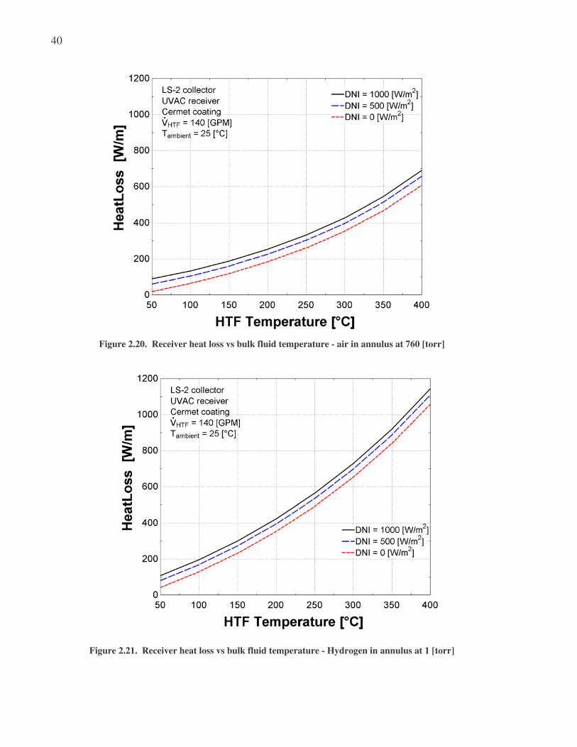
40

Figure 2.20. Receiver heat loss vs bulk fluid temperature - air in annulus at 760 [torr]

Figure 2.21. Receiver heat loss vs bulk fluid temperature - Hydrogen in annulus at 1 [torr]

41

The receiver heat loss model, as derived by Forristall, accounts for heat loss at a constant, fixed

bulk fluid temperature. As mentioned previously, the bulk temperature of the fluid will vary from

the field inlet to the field outlet by as much as 100 [°C]. To account for this temperature variance,

Equation 2.16 is integrated from field inlet temperature to field outlet temperature, and divided by

the difference in temperature between field inlet and field outlet:

O

I

T

T

Field

O I

HeatLoss

HLT T

=−

∫ (2.17)

2 2 3 3 4 4 3 331 2 10 0( ) ( ) ( ) ( ) [ ( ) ( )]

2 3 4 3( )

O I O I O I O I O I O I

Field

O I

aa a ba T T T T T T T T DNI b T T T T

HLT T

− + − + − + − + − + −=

− (2.18)

where

TO = Solar field temperature at the outlet [°C]

TI = Solar field temperature at the inlet [°C]

The final term for receiver heat loss is a weighted average of the heat loss resulting from each

type of HCE in the field:

,

1

NumHCETypesField i

i

i

HLRecHL HCEFrac

Width=

= ⋅∑ (2.19)

where Width = the width of the mirror aperture (5 [m] for LS-2 at SEGS VI)

42

Division by the mirror aperture width is performed to express the receiver heat loss as per unit of

mirror aperture area [W/m2].

2.3.3 Solar Field Piping Heat Losses

Thermal losses from the piping leading to and from the loops in the solar field are accounted for

by the following empirical equation (Price, 2005):

2 7 30.01693 0.0001683 6.78 10SfPipeHl T T T−= ∆ − ∆ + ⋅ ∆ (2.20)

where SfPipeHl is expressed per unit area of solar field aperture [W/m2], and ∆T [°C] is the

difference between the average field temperature and the ambient air temperature:

2

fieldoutlet fieldinlet

ambient

T TT T

+∆ = − (2.21)

Thermal losses due to piping to and from the solar field are generally small, on the order of 10

[W/m2] or less during solar field operation.

2.4 HTF Energy Gain and Temperature Rise

The net energy collected by the heat transfer fluid over the field, per unit aperture area [W/m2], is

the difference between the heat absorbed into the fluid by the absorber tubes ( absorbedQ� ,

Equation 2.1) and the sum of heat loss from the receivers (RecHL, Equation 2.19) and heat loss

from the piping to and from the solar field (SfPipeHl, Equation 2.20):

( )collected absorbedQ Q RecHl SfPipeHl= − +� � (2.22)

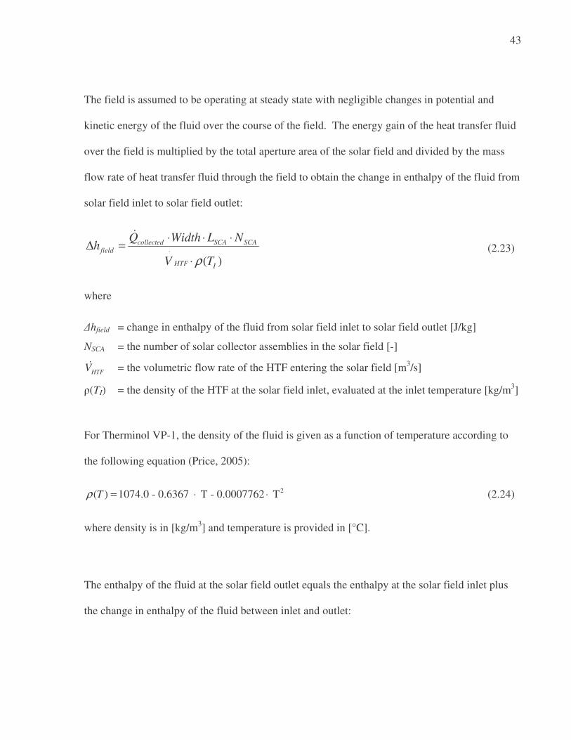
43

The field is assumed to be operating at steady state with negligible changes in potential and

kinetic energy of the fluid over the course of the field. The energy gain of the heat transfer fluid

over the field is multiplied by the total aperture area of the solar field and divided by the mass

flow rate of heat transfer fluid through the field to obtain the change in enthalpy of the fluid from

solar field inlet to solar field outlet:

( )

collected SCA SCAfield

HTF I

Q Width L Nh

V Tρ⋅

⋅ ⋅ ⋅∆ =

⋅

�

(2.23)

where

∆hfield = change in enthalpy of the fluid from solar field inlet to solar field outlet [J/kg]

NSCA = the number of solar collector assemblies in the solar field [-]

HTFV� = the volumetric flow rate of the HTF entering the solar field [m3/s]

ρ(TI) = the density of the HTF at the solar field inlet, evaluated at the inlet temperature [kg/m3]

For Therminol VP-1, the density of the fluid is given as a function of temperature according to

the following equation (Price, 2005):

2( ) 1074.0 - 0.6367 T - 0.0007762 TTρ = ⋅ ⋅ (2.24)

where density is in [kg/m3] and temperature is provided in [°C].

The enthalpy of the fluid at the solar field outlet equals the enthalpy at the solar field inlet plus

the change in enthalpy of the fluid between inlet and outlet:

44

( )out in I field

h h T h= + ∆ (2.25)

The enthalpy of Therminol VP-1 is a function of temperature according to the following equation

(Price, 2005):

2( ) 1000 (-18.34 + 1.498 T + 0.001377 T )h T = ⋅ ⋅ ⋅ (2.26)

where temperature (T) must be provided in [°C] and the enthalpy is returned in [J/kg]. It is

assumed that the enthalpy of the heat transfer fluid varies insignificantly with pressure.

Once the enthalpy of the heat transfer fluid at the solar field outlet is known, the temperature of

the fluid can be obtained from a temperature-enthalpy correlation for the HTF. For Therminol

VP-1, the temperature varies with enthalpy according to the function (Price, 2005):

2( ) -1.58E-10 + 0.0006072 + 13.37T h h h= ⋅ ⋅ (2.27)

where enthalpy is provided in [J/kg] and temperature is returned in [°C].

2.5 Heat Transfer Fluid Pumps

The heat transfer fluid is circulated by two variable speed driven heat transfer fluid pumps

operated in series (a third pump is included in the series as a standby). The speed of the pumps

is manually controlled by the plant operators. The heat transfer fluid pumping power is listed in

the technical evaluation as 1.6 [MWe] at design HTF flow, which is stated to be 7590 [gal/min]

at a temperature of 559 [°F] (293 [°C]) (Kearney et al, 1988). An efficiency of 0.60 is assumed

for the pumping process at the design flow; it is assumed that the pumps operate at their highest

efficiency at this design point. The pressure drop over the heat transfer fluid circulation loop at

45

design flow is estimated from the design flow rate, design pumping power, and the assumed

design efficiency of the pumps:

HTFpump HTFpump

HTF

HTF

WP

V

η ⋅∆ =

�

� (2.28)

This pressure drop estimate is based on the design pumping power requirements and does not

take into account the reductions in pressure drop that have been achieved at the SEGS plants

through operations and maintenance improvements, such as the ongoing replacement of flex

hoses at the ends of SCA rows with ball-joint assemblies (Cohen et al, 1999). The pressure drop

coefficient for the HTF circulation loop at design flow is determined from the calculated pressure

drop and design mass flow rate (the product of the volumetric flow rate and HTF density

evaluated at the design inlet temperature):

( )HTF

HTF

HTF inlet

Pk

V Tρ

∆=

⋅� (2.29)

The efficiency of the HTF pumping process at partial load flows is estimated as a function of

mass flow rate (Lippke, 1995):

2

, , ,

2(1 ) (1 )HTF HTF HTFmo mo mo

HTF ref HTF ref HTF ref

m me e e

m m

η

η

= + − − −

� �

� � (2.30)

where the subscript ‘ref’ refers to the value of the parameter at design conditions, and emo is a

dimensionless parameter that defines the shape of the efficiency curve. A value of emo =- 0.4 is

used in the work of Lippke (1995) and selected for the present investigation as well.

46

2.6 Model Capabilities and Limitations

The solar field model is computationally efficient and can be used to represent a solar field of

non-uniform composition. Over time, as older receiver tubes and mirrors wear down and break,

the field may be gradually replaced with the next generations of HCEs and mirrors. The makeup

of the solar field may include two or three or more types of solar collector assemblies and

receiver tubes. Surface properties and correction factors may vary from one brand or generation

of equipment to the next. The resultant efficiency for the field as a whole is assumed to be the

weighted average of the efficiency of each type of component found in the field.

The solar field is evaluated assuming steady state operation, with no accounting for thermal

capacitance. This assumption works fairly well through the majority of the operating day, but

creates some problems in the morning when the solar field is warming up. Without accounting

for thermal capacitance, the model predicts hotter temperatures at the solar field outlet in the

model than those actually realized. Thermal capacitance is accounted for in a separate storage

tank model (see Chapter 4).

In allowing the user to vary the properties of the HCEs and collectors in the field, the assumption

is made that each property contributes to the composite property of the field in proportion to its

prevalence in the field. The model does not allow the user to specify the location of

HCEs/collectors in the field, nor is there allowance to vary efficiencies or optical properties of

HCEs/collectors with local temperature in the affected equipment. There is no accounting, for

example, for the effects of using lower efficiency HCEs in the supply (cold) trough rows and

higher efficiency HCEs in the return (hot) trough rows.

47

3 Power Cycle Model

3.1 Introduction

In order to produce electricity, the thermal energy collected by the solar field must be converted

with an appropriate power cycle. The power cycle used in the SEGS plants is a traditional

Rankine cycle. This chapter describes the Rankine cycle used in the SEGS VI plant and presents

models for the power cycle components, which are based on energy and mass balances over the

components.

The power cycle begins by collecting the HTF returning from the solar field in an expansion

vessel. The expansion vessel serves to compensate for variation in the volume of the heat

transfer fluid throughout the day, since the specific volume of the HTF is dependent on

temperature. The heat transfer fluid is pumped from the expansion vessel and delivered to two

parallel heat exchanger trains (Train A and Train B) as the energy source for the power cycle.

Each of these heat exchanger trains consists of a superheater, steam generator, and feedwater

preheater, in series, as well as a reheater in parallel with the other three heat exchangers. Figure

3.1 depicts the flow of heat transfer fluid through the HTF – feedwater/steam heat exchangers.

48

Figure 3.1. Flow diagram for HTF through heat exchangers

For simplicity, the two parallel heat exchanger trains (Train A and Train B) are modeled as a

single train.

Figure 3.2 shows the flow diagram for the remainder of the SEGS VI Rankine power cycle. The

same diagram is reproduced in Figure 3.3, with state points labeled on the diagram. The state

points will be referred to throughout the remainder of the chapter.

Superheater Superheater

Reheater Reheater Steam Generator

Steam Generator

Preheater Preheater

HTF from solar field outlet

HTF to solar field inlet

Feedwater

Steam to HP turbine

Exhaust from HP turbine

Steam to LP turbine

Train A Train B

49

Figure 3.2. Flow diagram for power cycle - components labeled. The numbered vertical cylinders (#1 – 3, 5 –

6) represent closed feedwater heaters, while heater #4 represents the deaerator.

#1

#2

#3

#4

#5

#6

LP Turbine

HP Turbine

Condenser Pump

Deaerator Pump

Cooling Tower

Reheat

Superheat Preheat

Condenser

Steam Generation

Legend

Major steam line

Minor steam line Major feedwater line

Minor feedwater line Cooling water line

50

Figure 3.3. Flow diagram for power cycle - state points labeled.

The HTF receives pre-heated feedwater and generates dry steam at a temperature and pressure of

371 [°C] and 100 [bar] (at rated power conditions) by heat exchange with the HTF in the steam

preheater, steam generator, and superheater. The superheated steam travels first through the high

pressure turbine, where it expands and propels the turbine blades. Two extractions are taken

from the high pressure turbine; these extracted steam lines are used to preheat feedwater in two

closed feedwater heaters (#5 and #6). Upon exiting the high pressure turbine, the steam is

directed through a reheater, where it is superheated to approximately the same temperature

reached at the outlet of the superheater and a pressure of about 17.5 [bar] (at rated power

[42]

[22] [21]

[43]

[12]

[13]

[14]

[15]

[16]

[17]

[18]

[19]

[20]

[10]

[11]

[30]

[29]

[9]

[8]

[7]

[6]

[5]

[4]

[3]

[2]

[1]

[23]

[24]

[25]

[26]

[27]

[28]

[40]

[45] [46]

[41] [44]

[46]

[47]

Legend

Major steam line

Minor steam line

Major feedwater line Minor feedwater line

Cooling water line

51

conditions). The superheated steam then passes through the low pressure turbine, where again

the steam expands and propels the turbine blades. Four steam extractions are taken from the low

pressure turbine; one is directed to the deaerator (feedwater heater #4), and the remaining three

are fed to feedwater heaters #1 – #3. The steam leaving the low pressure turbine is condensed in

a surface condenser by heat exchange with circulating water. The condenser water is cooled

using an induced draft cooling tower. The condensed steam (now referred to as feedwater) is

pumped to a sufficiently high pressure (15 [bar]) to allow it to pass through the three low

pressure feedwater heaters and into the deaerator. The feedwater is pumped again at the outlet of

the deaerator, to a pressure slightly higher than the boiling pressure in the steam generator (125

[bar], at rated power conditions). Feedwater passes through the two high pressure feedwater

heaters before returning to the preheater to complete the cycle.

3.2 Temperature – Entropy Diagram

The temperature, pressure, enthalpy, and mass flow rate at each state point in the system for its

rated power load of 35 [MWe] gross power with 100% solar operation are provided in the

technical feasibility assessment of the plant (Kearney et al, 1988). This state is referred to as the

‘reference’ state for the power plant. A temperature – entropy diagram of the cycle with all

corresponding intermediate state points at the reference condition is shown in Figure 3.4.

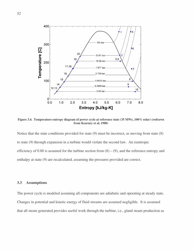
52

Figure 3.4. Temperature-entropy diagram of power cycle at reference state (35 MWe, 100% solar) (redrawn

from Kearney et al, 1988)

Notice that the state conditions provided for state (9) must be incorrect, as moving from state (8)

to state (9) through expansion in a turbine would violate the second law. An isentropic

efficiency of 0.88 is assumed for the turbine section from (8) – (9), and the reference entropy and

enthalpy at state (9) are recalculated, assuming the pressures provided are correct.

3.3 Assumptions

The power cycle is modeled assuming all components are adiabatic and operating at steady state.

Changes in potential and kinetic energy of fluid streams are assumed negligible. It is assumed

that all steam generated provides useful work through the turbine, i.e., gland steam production as

53

well as steam losses through line leaks are neglected. Also, negligible changes in fluid state

between the outlet of one component and the inlet of the next are assumed.

Correlations are provided by the National Renewable Energy Laboratory (Price, 2005) for the

heat transfer fluid (Therminol VP-1) properties as a function of temperature. It is assumed that

the fluid properties (enthalpy, density, and specific heat) do not have any significant dependence

on pressure.

In the condenser and feedwater heaters, the condensing steam outlet is located beneath the steam

inlet. Flow is held at steady state by maintaining a constant condensate level in the component.

Thus, steam vapor can not exit the component. In the steam generator, the opposite situation

occurs; the steam generator fluid exit is located above the inlet, and with a constant feedwater

level in the generator, saturated liquid can not exit. In addition to the aforementioned

assumptions, which apply to all power cycle components, the following assumptions are made

for these specific components:

• Preheater: feedwater exits the preheater as saturated liquid (x = 0)

• Steam generator: steam exits the steam generator as saturated vapor (x = 1)

• Closed feedwater heaters: condensed steam exits the heater as saturated liquid (x = 0)

• Open feedwater heater: feedwater exits the deaearator as saturated liquid (x = 0)

• Condenser: feedwater exits the condenser as saturated liquid (x = 0)

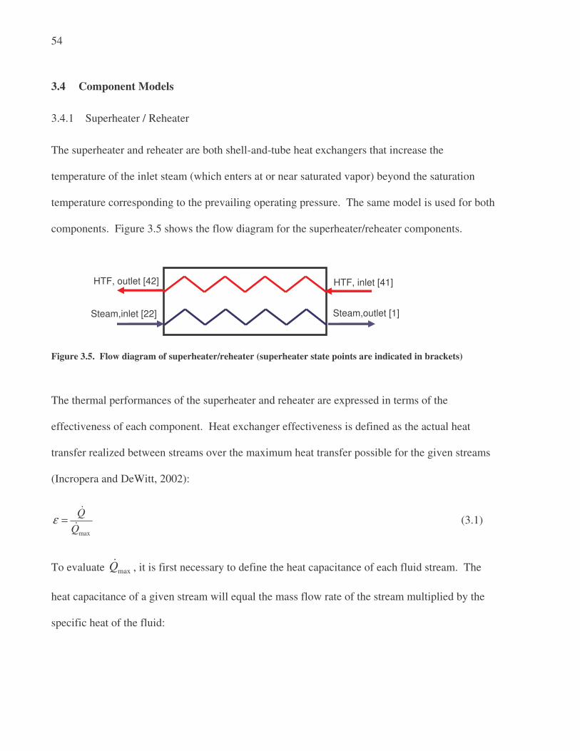
54

3.4 Component Models

3.4.1 Superheater / Reheater

The superheater and reheater are both shell-and-tube heat exchangers that increase the

temperature of the inlet steam (which enters at or near saturated vapor) beyond the saturation

temperature corresponding to the prevailing operating pressure. The same model is used for both

components. Figure 3.5 shows the flow diagram for the superheater/reheater components.

Figure 3.5. Flow diagram of superheater/reheater (superheater state points are indicated in brackets)

The thermal performances of the superheater and reheater are expressed in terms of the

effectiveness of each component. Heat exchanger effectiveness is defined as the actual heat

transfer realized between streams over the maximum heat transfer possible for the given streams

(Incropera and DeWitt, 2002):

max

Q

Qε =

�

� (3.1)

To evaluate maxQ� , it is first necessary to define the heat capacitance of each fluid stream. The

heat capacitance of a given stream will equal the mass flow rate of the stream multiplied by the

specific heat of the fluid:

HTF, inlet [41]

Steam,outlet [1]

HTF, outlet [42]

Steam,inlet [22]

55

C steam steamC m cp= ⋅� � (3.2)

H HTF HTFC m cp= ⋅� � (3.3)

where

CC� = capacitance rate of the cold side fluid (steam) [kW/K]

HC� = capacitance rate of the hot side fluid (HTF) [kW/K]

,steam HTFm� = mass flow rate of the steam or HTF (41) [kg/s]

steamcp = average specific heat of steam between inlet and outlet [kJ/kg-K]

HTFcp = average specific heat of HTF between inlet and outlet [kJ/kg-K]

The average specific heat for each stream is the difference in enthalpy of the stream between

inlet and exit, divided by the temperature difference between inlet and exit.

, ,

, ,

steam out steam in

steam

steam out steam in

h hcp

T T

−=

− (3.4)

, ,

, ,

HTF out HTF in

HTF

HTF out HTF in

h hcp

T T

−=

− (3.5)

The maximum heat transfer possible between streams will equal the smaller total heat

capacitance of the two fluid streams, multiplied by the difference in inlet temperatures between

the streams.

max min , ,( )HTF in steam inQ C T T= −� (3.6)

where

min ( , )C HC MIN C C= � � (3.7)

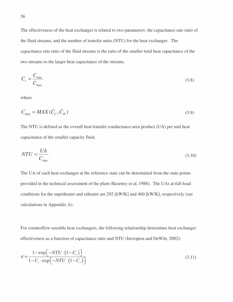
56

The effectiveness of the heat exchanger is related to two parameters: the capacitance rate ratio of

the fluid streams, and the number of transfer units (NTU) for the heat exchanger. The

capacitance rate ratio of the fluid streams is the ratio of the smaller total heat capacitance of the

two streams to the larger heat capacitance of the streams.

min

max

r

CC

C= (3.8)

where

max ( , )C H

C MAX C C= � � (3.9)

The NTU is defined as the overall heat transfer conductance-area product (UA) per unit heat

capacitance of the smaller capacity fluid.

min

UANTU

C= (3.10)

The UA of each heat exchanger at the reference state can be determined from the state points

provided in the technical assessment of the plant (Kearney et al, 1988). The UAs at full-load

conditions for the superheater and reheater are 292 [kW/K] and 460 [kW/K], respectively (see

calculations in Appendix A).

For counterflow sensible heat exchangers, the following relationship determines heat exchanger

effectiveness as a function of capacitance ratio and NTU (Incropera and DeWitt, 2002):

( )

( )

1 exp 1

1 exp 1

r

r r

NTU C

C NTU C

− − ⋅ − ε =− ⋅ − ⋅ −

(3.11)

57

Once maxQ� and the effectiveness have been calculated, the actual heat transfer between fluid

streams is determined from Equation (3.1).

The exit enthalpy of the steam is determined from the inlet enthalpy of the steam plus the heat

transfer per unit steam mass flow rate:

, ,steam out steam in

steam

Qh h

m= +

�

� (3.12)

Outlet temperature is determined from the outlet enthalpy and outlet pressure of the steam:

, , ,T( , )steam out steam out steam outT h P= (3.13)

where the outlet pressure is equal to the inlet pressure minus the pressure drop coefficient times

the mass flow rate of the steam, squared (Moran and Shapiro, 2001):

2

, ,steam out steam in steam steamP P k m= − ⋅ � (3.14)

Solving Equation (3.14) for the pressure drop coefficient ksteam, given the inlet pressure, outlet

pressure, and mass flow rate provided at the reference state, the pressure drop coefficients are

found to be 0.0023 [bar-s2/kg2] for the superheater and 0.001 [bar-s2/kg2] for the reheater (see

calculations in Appendix A).

The exit enthalpy of the HTF is determined from an energy balance on the fluid:

, ,HTF out HTF in

HTF

Qh h

m= −

�

� (3.15)

58

Outlet temperature of the heat transfer fluid may be determined as a function of enthalpy by

solving the cubic equation proposed by Price (2005):

2 3 = 1.49937 + (0.00269436/2) + (0.000000165426/3)HTF HTF HTF HTFh T T T (3.16)

where hHTF is provided in [kJ/kg] and THTF is in [°C].

Continuity requires the mass flow rates of the HTF and steam at the respective outlets to equal

the mass flow rates of each steam at their inlet.

, ,steam in steam outm m=� � (3.17)

, ,HTF in HTF outm m=� � (3.18)

The UA for the heat exchanger at the reference state is provided as a parameter to the exchanger

model. At partial loads, the UA will decrease with the decreasing flow rates of the streams. The

relationship between the reference UA/flow rate and a reduced UA/flow rate can be derived as

follows. The UA of an unfinned, tubular heat exchanger is defined as the total thermal resistance

to heat transfer between two fluids (Incropera and Dewitt, 2002):

" "ln1 1 1

2

fi foo i

i i i o o o

R RD D

UA h A A kL A h Aπ= + + + + (3.19)

where

h = convection heat transfer coefficient [W/m2-K]

A = surface area [m2]

R” = fouling factor, per unit area [m2-K/W]

D = diameter [m]

k = thermal conductivity of the material between the fluids [W/m-K]

59

L = length of the heat exchanger [m]

i (subscript) = property of the inner surface of the heat exchanger

o (subscript) = property of the outer surface of the heat exchanger

Equation (3.19) can be simplified if it is assumed that there is negligible fouling in the heat

exchangers and that the thermal resistance through the tubes can be neglected. With these

assumptions, Equation (3.19) reduces to:

1 1 1

i i o oUA h A h A= + (3.20)

In Equation (3.20), UA is a function of the inner and outer surface areas of the tubes and the heat

transfer coefficient of each fluid. The surface area of the tubes will not change with partial load

conditions. The heat transfer coefficients are a function of the Nusselt number:

fluidNu kh

D

⋅= (3.21)

where

Nu = the Nusselt number

kfluid = the thermal conductivity of the fluid

D = the hydraulic diameter

Assuming that the flow for both fluids is fully developed (hydrodynamically and thermally) and

turbulent through smooth circular tubes, the Nusselt number can be expressed as a function of

the Reynolds number (Re) and Prandtl number (Pr) by:

0.80.023 Re Prn

D DNu = ⋅ ⋅ (3.22)

where n = 0.4 for heating fluid and n = 0.3 for cooling fluid.

60

Definitions of the Reynolds number and the Prandtl number complete the equations:

4ReD

m

Dπ µ

⋅=

i

(3.23)

where

µ = dynamic fluid viscosity [N-s/m2]

Prfluid

c

k

µ ⋅= (3.24)

where

c = specific heat of fluid [kJ/kg-K]

Assuming constant fluid properties, the Prandtl number will be constant for each fluid, and the

Reynolds number will vary only with mass flow rate of the fluid. From Equation (3.21), the heat

transfer coefficient is proportional to the Nusselt number. Therefore, assuming constant fluid

properties, the heat transfer coefficient is proportional to the mass flow rate raised to the 0.8

power:

0.8 0.8Reh Nu h h m∝ ⇒ ∝ ⇒ ∝ � (3.25)

From Equation (3.20), the UA of a heat exchanger must be proportional to the fluid stream mass

flow rate as follows:

0.8 0.8

1 1 1

i oUA m m∝ +� �

(3.26)

The same correlation can be written for the reference UA, as a function of its reference inner and

outer fluid mass flow rates:

61

0.8 0.8

, .

1 1 1

REF i REF o REFUA m m∝ +� �

(3.27)

Combining Equations (3.26) and (3.27), the partial load UA and mass flow rates relate to the

reference UA and mass flow rates through the following relationship:

0.8 0.8 0.8 0.80.8 0.8, . . ,

0.8 0.8 0.8 0.8

, .0.8 0.8

1 1

1 1i REF o REF o REF i REFi o

REF i REF o REF o i

i o

m m m mm mUA

UA m m m m

m m

+ +⋅

= = ⋅ + +

� � � ��

� � � �

� �

(3.28)

Finally, it is assumed that the mass flow rates of the inner and outer fluids remain in the same

proportion at partial load conditions as at the reference load so that:

,

.

i REFi

o o REF

mmK

m m= =��

� � (3.29)

Substituting Equation (3.29) into Equation (3.28) and simplifying the terms, Equation (3.28)

reduces to

0.8 0.8

, .

0.8 0.8

1 1

1 1o REF o REF

REF

o o

KK m mUA

UA

K m m

+⋅

= =

+⋅

� �

� �

0.8 0.8

o om m⋅ ⋅� �

K0.8 0.8

, .o REF o REFm m⋅ ⋅� �

0.8

,o REFm

� ( 1)K +

0.8

om� ( 1)K +

(3.30)

Further simplification of Equation (3.30) results in the desired relation.

0.8

,

o

REF o REF

mUA

UA m

=

�

� (3.31)

62

3.4.2 Steam Generator (Boiler)

The steam generator is a shell-and-tube heat exchanger with liquid feedwater on the shell side

and hot HTF through the tube side. Feedwater boils on the surface of the HTF tubes and rises to

exit the steam generator as saturated vapor. The flow through the steam generator is controlled

such that a constant feedwater level is maintained in the vessel. Figure 3.6 shows the flow

diagram for the steam generator.

Figure 3.6. Flow diagram of steam generator (state points are indicated in brackets)

The effectiveness of the steam generator is determined from an effectiveness/NTU relationship,

in which the effectiveness and the number of transfer units (NTU) are as defined in Equations

(3.1) and (3.10), respectively. In changing phase from saturated liquid to saturated vapor, the

heat capacitance of the feedwater/steam is infinite; therefore, the minimum capacitance of the

two fluids as defined by Equation (3.7) will always be the capacitance of the hot side fluid (the

heat transfer fluid):

, ,

, ,

HTF in HTF out

MIN HTF

HTF in HTF out

h hC m

T T

−= − � (3.32)

Given that the heat capacitance of the feedwater/steam is effectively infinite, the capacitance

ratio as defined in Equation (3.8) for this heat exchanger is zero. Under these conditions, the

HTF, inlet [42]

Steam,outlet [22] X=1

HTF, outlet [43]

Feedwater,inlet [21] X=0

63

appropriate effectiveness/NTU relationship for the heat exchanger is (Incropera and Dewitt,

2002):

1 exp( )NTUε = − − (3.33)

The boiling temperature, HTF inlet and outlet temperature, and mass flow rates are specified at

rated power for 100% solar load in the technical assessment; from these values, the UA of the

steam generator at the reference state is found to be 2051 [kW/K] (see calculations in Appendix

A). This UA is adjusted for partial load conditions using Equation (3.31).

The exit enthalpy of the steam is assumed to be that of saturated vapor at the inlet pressure to the

steam generator (assume no pressure drop over the steam generator):

, ,steam in steam outP P= (3.34)

, ,( , 1)steam out steam outh h P x= = (3.35)

The mass flow rate of feedwater/steam through the steam generator may be determined from the

heat transfer between fluids over the difference in enthalpy from feedwater inlet to steam outlet:

( ),

, ,

steam out

steam out feedwater in

Qm

h h=

−

�

� (3.36)

The exit enthalpy of the HTF is determined from the inlet enthalpy of the HTF minus the heat

transfer per unit HTF mass flow rate:

, ,HTF out HTF in

HTF

Qh h

m= −

�

� (3.37)

64

Outlet temperature of the heat transfer fluid may be determined as a function of enthalpy by the

correlation given in Equation (3.16).

The mass flow rates of the HTF and steam at the outlet will equal the mass flow rates of the

streams at the inlet.

, ,feedwater in steam outm m=� � (3.38)

, ,HTF in HTF outm m=� � (3.39)

3.4.3 Preheater

The preheater raises the temperature of the feedwater from its temperature at the outlet of heater

#6 to its saturation temperature at the preheater outlet pressure. Figure 3.7 shows the flow

diagram for the HTF – steam preheater.

Figure 3.7. Flow diagram of preheater (state points are indicated in brackets)

The preheater is modeled assuming that the feedwater exit state will be saturated liquid at the

outlet pressure of the preheater. Outlet pressure of the feedwater is calculated as the inlet

pressure minus the pressure drop coefficient multiplied by the square of the mass flow rate:

HTF, inlet [43]

Feedwater,outlet [21]

HTF, outlet [44]

Feedwater,inlet [20]

65

2

, ,feedwater out feedwater in feedwater feedwaterP P k m= − ⋅ � (3.40)

, ,( , 0)feedwater out feedwater outh h P x= = (3.41)

The pressure drop coefficient, kfeedwater , is found from inlet and outlet pressures and mass flow

rates provided for the reference state of the plant to be 0.000092 [bar-s2/kg2] (see Appendix A).

The heat transfer to the feedwater is calculated, given the feedwater mass flow rate and the

known inlet and outlet states of the feedwater:

, ,( )feedwater feedwater out feedwater inQ m h h= −� � (3.42)

For an adiabatic heat exchanger, the heat transfer to the feedwater must equal the heat transfer

from the HTF. The exit enthalpy of the HTF (and consequently the HTF exit temperature) is

determined from the heat transfer between streams and the HTF mass flow rate:

, ,HTF out HTF in

HTF

Qh h

m= −

�

� (3.43)

Outlet temperature of the heat transfer fluid is determined from outlet enthalpy using the

correlation from Equation (3.16).

Notice that, unlike heat exchanger models previously discussed, the UA of the preheater is not

specified. In effect, the assumption is made that the preheater is of variable length as needed to

raise the feedwater temperature to boiling temperature but not begin to boil the fluid. In the

actual heat exchanger train, the exit state of the preheater is not so clearly defined. It is likely

that some feedwater preheating occurs in the steam generator, or that a small amount of steam

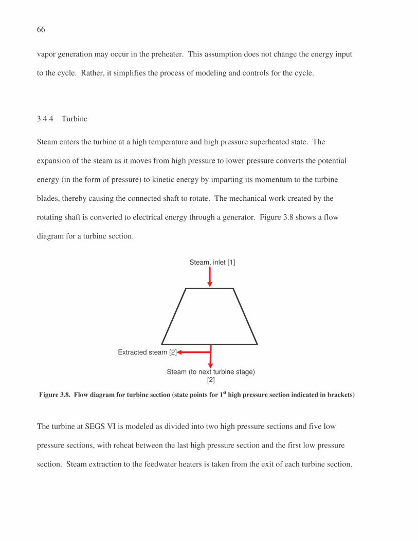
66

vapor generation may occur in the preheater. This assumption does not change the energy input

to the cycle. Rather, it simplifies the process of modeling and controls for the cycle.

3.4.4 Turbine

Steam enters the turbine at a high temperature and high pressure superheated state. The

expansion of the steam as it moves from high pressure to lower pressure converts the potential

energy (in the form of pressure) to kinetic energy by imparting its momentum to the turbine

blades, thereby causing the connected shaft to rotate. The mechanical work created by the

rotating shaft is converted to electrical energy through a generator. Figure 3.8 shows a flow

diagram for a turbine section.

Figure 3.8. Flow diagram for turbine section (state points for 1st high pressure section indicated in brackets)

The turbine at SEGS VI is modeled as divided into two high pressure sections and five low

pressure sections, with reheat between the last high pressure section and the first low pressure

section. Steam extraction to the feedwater heaters is taken from the exit of each turbine section.

Extracted steam [2]

Steam, inlet [1]

Steam (to next turbine stage) [2]

67

The performance of each section is defined by its isentropic efficiency. The isentropic efficiency

of a turbine stage is the ratio of the change in enthalpy of the fluid to the change that would have

occurred in an isentropic (reversible) turbine:

, ,

, , ,

steam in steam out

turbine

steam in steam out S

h h

h hη

−=

− (3.44)

where hsteam,out,S is the enthalpy that would have occurred at the outlet of the turbine were it an

isentropic process. This ideal enthalpy is evaluated using the outlet pressure and inlet entropy of

the fluid:

, , , ,( , )steam out s steam out steam inh h P s= (3.45)

The pressure and enthalpy at the inlet and exit of each turbine section are given in the reference

state parameters supplied in the technical assessment (Kearney et al, 1988). Table 3.1 shows the

reference inlet and outlet pressure and reference state efficiency of each section. The turbine

section efficiencies at the reference state were calculated from these values (see Appendix A).

Table 3.1. Reference efficiency and pressures for turbine sections

(Source: Kearney et al, 1988)

Turbine

Section

Inlet Pressure

[bar]

Exit Pressure

[bar]

Efficiency

[1] – [2] 100 33.61 0.8376

[2] – [3] 33.61 18.58 0.8463

[5] – [6] 17.10 7.98 0.8623

[6] – [7] 7.98 2.73 0.917

[7] – [8] 2.73 0.96 0.9352

[8] – [9] 0.96 0.29 0.88*

[9] – [10] 0.29 0.08 0.6445 *Isentropic efficiency calculated from reference pressures and enthalpies was >1; the value shown was assumed.

68

The efficiency of turbine stages will vary at partial loads as compared to its design load. The

SEGS VI turbines are 3600 rpm, condensing turbines, with one impulse stage and the remainder

reaction stages, with a reheat section between the high pressure and low pressure turbines (SEGS

VI Engineering Handbook, 1986). Figure 3.9 shows the percent reduction in efficiency as a

function of throttle flow ratio for a 3600-rpm condensing turbine with one governing stage

(Bartlett, 1958):

Figure 3.9. Percent reduction in efficiency as a function of throttle flow ratio, for condensing turbine with

one governing stage (Source: Adapted from Bartlett, 1958)

The efficiency of the turbine is expressed as a function of the reference efficiency for the section

and the throttle flow ratio:

(1 % ) refReductionη η= − ⋅ (3.46)

69

where %Reduction is expressed as a function of the ratio of the mass flow of steam through the

section over the mass flow through the section at the reference state, using the equation presented

in Figure 3.9.

The pressure drop over each turbine section will vary with the mass flow rate of steam as well.

The law of the ellipse governs the relationship between turbine inlet pressure, outlet pressure,

and mass flow rate at partial load, as compared to some reference load (Stodola and Lowenstein,

1945):

22 2

1 2

2 2

1, 2,ref ref ref

P P m

P P m

−= −

�

� (3.47)

If any two properties are known, the value of the third property may be found from Equation

(3.47). In the SEGS plant, the mass flow rate of steam is fixed by the steam generator, and the

exhaust pressure of the low pressure turbine (equal to the condensing pressure) is an input to the

model. The inlet pressure to each section is determined from Equation (3.47), provided the mass

flow rate through the section and the exhaust pressure of the section.

The work per unit mass performed by the turbine stage is equal to the change in fluid enthalpy

over the turbine stage:

1 2 1 2( )w h h− = −� (3.48)

At the exit of each section, a fraction of the mass flow rate through the section is extracted and

used to preheat feedwater to the boiler. The mass flow of steam demanded by each feedwater

heater is determined through the feedwater heater models. The mass flow continuing to the next

70

turbine section is the mass flow into the turbine minus the mass flow of any extractions previous

to that section.

3.4.5 Condenser

Upon exiting the low pressure turbine, the working fluid proceeds to the condenser, located

beneath the turbine. The condenser is a closed shell-and-tube heat exchanger, with cooling water

flow on the tube side and condensing steam from the turbine on the shell side. The function of

the condenser is to condense the turbine exhaust from vapor to liquid, so the working fluid can

be pumped back to the boiler. Figure 3.10 shows the flow diagram for the condenser.

Figure 3.10. Flow diagram of condenser (state points indicated in brackets)

It is assumed that there is no pressure drop in the steam side of the condenser, and that no

subcooling occurs in the condenser. The enthalpy of the steam at the condenser outlet equals the

saturated liquid enthalpy at the condensing pressure:

Condensed feedwater, outlet [12]

X=0

Steam, inlet [11]

Cooling water, inlet Cooling water, outlet

71

, ,steam in feedwater outP P= (3.49)

, ,( , 0)feedwater out feedwater outh h P x= = (3.50)

The condensing pressure is provided as an input to the power cycle model. The condensing

pressure is determined in an external model from the overall conductance-area (UA) of the

condenser, as well as the mass flow rate and enthalpy into the condenser and the mass flow rate

and enthalpy of the incoming circulating cooling water. The condenser supply water temperature

to the cycle is dictated by the performance of the cooling tower and the outside air wet bulb

temperature. The performances of the condenser and cooling tower are modeled external to the

power cycle model. Equations for modeling the condenser and cooling tower performance to

predict the condensing pressure are discussed in Chapter 4.

3.4.6 Pump

The pumps in the cycle serve to increase the pressure of the working fluid. There are two

pumping processes on the working fluid side of the power cycle. One set of pumps is located at

the condenser outlet, to pump the fluid from its condensing pressure to flow through the low

pressure feedwater heaters and deaerator. Another set of pumps is located at the deaerator outlet,

to pump the fluid from the extraction pressure to the high pressures required at the boiler inlet.

Figure 3.11 shows the flow diagram for a pump.

72

Figure 3.11. Flow diagram of a pump (state points for the condenser pump indicated in brackets)

Pump performance is characterized by its isentropic efficiency. The isentropic efficiency of the

pump is the ratio of the isentropic (reversible) change in enthalpy of the fluid to the change in

enthalpy that actually occurred:

, , ,S

, ,

feedwater in feedwater out

pump

feedwater in feedwater out

h h

h hη

−=

− (3.51)

where hfeedwater,out,S is the enthalpy that would have occurred were the pumping process

isentropic. This ideal enthalpy is evaluated using the desired outlet pressure and inlet entropy of

the fluid:

, ,S , ,( , )feedwater out feedwater out feedwater inh h P s= (3.52)

A reference isentropic efficiency of 0.6 (including both pump efficiency and motor efficiency) is

assumed for both pumps. The pump efficiency will change with changing load conditions.

Assume the pumps operate at maximum efficiency at the reference state. For constant speed

pumps, the change in pump efficiency is expressed as a function of the change in mass flow rate

by (Lippke, 1995)

Feedwater, outlet [13] Feedwater, inlet [12]

73

2

,

2pump

pump ref ref ref

m m

m m

η

η

= ⋅ −

i i

i i (3.53)

The work performed by the pump per unit mass is the change in fluid enthalpy from inlet to

outlet:

, ,pump feedwater in feedwater outw h h= −i

(3.54)

Note that the enthalpy of the feedwater at the inlet will always be lower than the enthalpy of the

feedwater at the outlet, and thus values for pump work are negative with the sign convention

assumed here.

3.4.7 Closed Feedwater Heater

A closed feedwater heater is a shell-and-tube heat exchanger with high pressure feedwater in the

tube side and condensing steam extracted from the turbine on the shell side. In essence, a closed

feedwater heater is a small condenser that operates at much higher pressure than the main

condenser (El-Wakil, 1984). Closed feedwater heaters are added to the cycle to preheat the

steam generator feedwater. While steam extraction for feedwater heating decreases the power

output of the turbine, it also increases the temperature of the feedwater to the boiler, reducing the

need for heat addition from the solar field and increasing the efficiency of the cycle. Figure 3.12

shows the flow diagram for a closed feedwater heater.

74

Figure 3.12 Flow diagram for a closed feedwater heater (state points are shown in brackets, using heater #6

as an example)

Heat transfer in the closed feedwater heater will occur through three zones; the desuperheating

zone, in which the steam is reduced to saturated vapor, the condensing zone, in which the steam

condenses from saturated vapor to saturated liquid, and a subcooling or drain cooling zone, in

which the condensed steam is cooled to a temperature below its saturation temperature. The size

and conductance of heat exchangers are characterized by an overall heat transfer coefficient

(UA). Each zone in the closed feedwater heater will have an associated UA value. It is assumed

here that the condensing zone of each feedwater heater is sufficiently large in comparison to the

desuperheating and subcooling zones that the desuperheating and subcooling zones can be

neglected. An overall UA for each feedwater heater is defined assuming steam is condensing

throughout the length of the feedwater heater.

Condensed steam, outlet [23]

X=0

Steam, inlet [2]

Feedwater, inlet [19]

Feedwater, outlet [20]

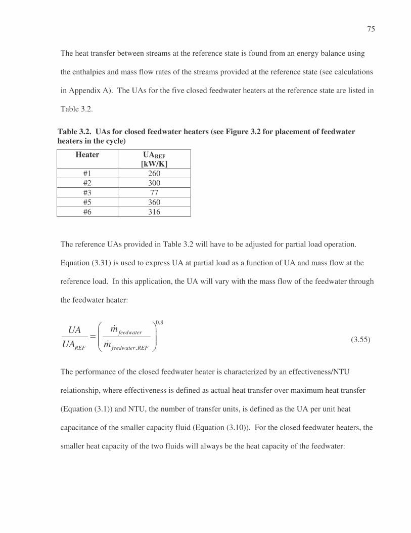
75

The heat transfer between streams at the reference state is found from an energy balance using

the enthalpies and mass flow rates of the streams provided at the reference state (see calculations

in Appendix A). The UAs for the five closed feedwater heaters at the reference state are listed in

Table 3.2.

Table 3.2. UAs for closed feedwater heaters (see Figure 3.2 for placement of feedwater

heaters in the cycle)

Heater UAREF

[kW/K]

#1 260

#2 300

#3 77

#5 360

#6 316

The reference UAs provided in Table 3.2 will have to be adjusted for partial load operation.

Equation (3.31) is used to express UA at partial load as a function of UA and mass flow at the

reference load. In this application, the UA will vary with the mass flow of the feedwater through

the feedwater heater:

0.8

,

feedwater

REF feedwater REF

mUA

UA m

=

�

� (3.55)

The performance of the closed feedwater heater is characterized by an effectiveness/NTU

relationship, where effectiveness is defined as actual heat transfer over maximum heat transfer

(Equation (3.1)) and NTU, the number of transfer units, is defined as the UA per unit heat

capacitance of the smaller capacity fluid (Equation (3.10)). For the closed feedwater heaters, the

smaller heat capacity of the two fluids will always be the heat capacity of the feedwater:

76

, ,

, ,

feedwater out feedwater in

MIN feedwater

feedwater out feedwater in

h hC m

T T

−= − � (3.56)

For a heat exchanger in which one fluid undergoes a phase change, the ratio of minimum to

maximum fluid heat capacities is zero, and the effectiveness/NTU relationship is given in

Equation (3.33).

The exit enthalpy of the condensed steam (condensate) is that of saturated liquid at the inlet

pressure to the feedwater heater, assuming that no pressure drop occurs over the condensing

steam:

, ,steam in steam outP P= (3.57)

, ,( , 0)steam out steam outh h P x= = (3.58)

The mass flow rate of extracted steam/condensate through the heater may be determined from

the heat transfer between fluids over the difference in enthalpy from steam inlet to condensate

outlet:

( ), ,

steam

steam in steam out

Qm

h h=

−

�

� (3.59)

The exit enthalpy of the feedwater is determined from the inlet enthalpy of the feedwater plus the

heat transfer per unit feedwater mass flow rate:

, ,feedwater out feedwater in

feedwater

Qh h

m= +

�

� (3.60)

77

The outlet feedwater temperature may be determined as a function of the outlet pressure and

outlet enthalpy using a property relation for water:

, , ,T( , )feedwater out feedwater out feedwater outT P h= (3.61)

The mass flow rates of the feedwater and steam/condensate at the outlet will equal the mass flow

rates of the streams at the inlet.

, ,feedwater in feedwater outm m=� � (3.62)

, ,steam in steam outm m=� � (3.63)

3.4.8 Open Feedwater Heater (Deaerator)

The open feedwater heater, like the closed feedwater heaters, uses extracted steam from the

turbine to preheat feedwater to the steam generator. Unlike the closed feedwater heaters,

however, in the open feedwater heater the extracted steam is directly mixed with the feedwater.

Open feedwater heaters are more effective than closed feedwater heaters, and are beneficial for

the removal of noncondensables from the feedwater (El-Wakil, 1984). The disadvantage of open

feedwater heaters is that the outlet pressure cannot exceed the pressure of the extracted steam; an

additional pump is required at the feedwater exit to increase fluid pressure to boiling pressure.

Figure 3.13 shows the flow diagram for the open feedwater heater.

78

Figure 3.13. Open feedwater heater diagram (state points are indicated in brackets)

The open feedwater heater is modeled as a fluid mixer with three inlet streams and a single outlet

stream. The three inlet streams are the extracted steam from the first stage of the low pressure

turbine (state [6]), the drain water from the high pressure feedwater heaters (state [25]), and the

feedwater from the low pressure feedwater heaters (state [16]). The mass flow rate of the outlet

stream is the sum of the mass flow rates of the three inlet streams:

, , , ,steam extracted steam drain feedwater in feedwater outm m m m+ + =� � � � (3.64)

An energy balance indicates that the enthalpy of the feedwater at the outlet is equal to the

weighted average of the enthalpies of the three streams entering the heater:

, , , ,extract extract drain drain feed in feed in feed out feed outm h m h m h m h⋅ + ⋅ + ⋅ = ⋅� � � � (3.65)

Assuming that the feedwater exits as saturated liquid (x = 0), the enthalpy of the outlet is also

equal to the saturated liquid enthalpy at the outlet pressure:

, ,( , 0)feed out feed outh h P x= = (3.66)

Drain steam [25]

Feedwater, inlet [16]

Feedwater, outlet [17]

Extracted steam [6]

79

where the pressure at the feedwater outlet is assumed to be the pressure of the extracted steam

(the outlet pressure cannot exceed this pressure):

, ,feedwater out steam extractedP P= (3.67)

Enthalpy and mass flow at state [26] and [16] are inputs to the open feedwater heater model, as

well as enthalpy at state [6] and mass flow at state [17]. The mass flow rate at state [6] is

determined by simultaneous solution of Equations (3.64) through (3.66).

Since the outlet state is saturated liquid, the temperature at the heater outlet is the saturation

temperature at the outlet pressure:

, ,T_SAT( )feedwater out feedwater outT P= (3.68)

3.4.9 Mixer

Drain water (condensed steam) from the closed feedwater heaters is cascaded backward,

meaning the condensed steam drained from one feedwater heater is fed back to the hot side inlet

of the next lower-pressure feedwater heater (El-Wakil 53). For example, the drain from heater

#6 (state [23]) mixes with extracted steam (state [3]) to produce a stream of saturated steam and

hot water. This mixture becomes the hot inlet for heater #5 (state [24]). The mixer models this

mixing of drain water and extracted steam. Figure 3.14 shows the flow diagram for the mixer.

80

Figure 3.14. Flow diagram of mixer (state points for mixer preceding heater #5 are indicated in brackets)

The mixer has two inlet streams and a single outlet stream. The mass flow rate at the outlet of

the mixer is the sum of the mass flow rates of the two inlet streams:

, ,in steam in feedwater outm m m+ =� � � (3.69)

An energy balance indicates that the enthalpy of the outlet is the weighted average of the

enthalpies of the two inlet streams:

, , , ,in steam in steam in feedwater in feedwater out outm h m h m h⋅ + ⋅ = ⋅� � � (3.70)

The pressure at the outlet is assumed to be equal to the pressure of the extracted steam line:

,in steam outP P= (3.71)

Since the mixture of drain water and extracted steam will always produce a saturated mixture,

the temperature of the outlet stream is calculated as the saturation temperature at the pressure of

the extracted steam line:

T_SAT( )out outT P= (3.72)

Extracted steam [3]

Mixed outlet [24]

Condensed drain steam [23]

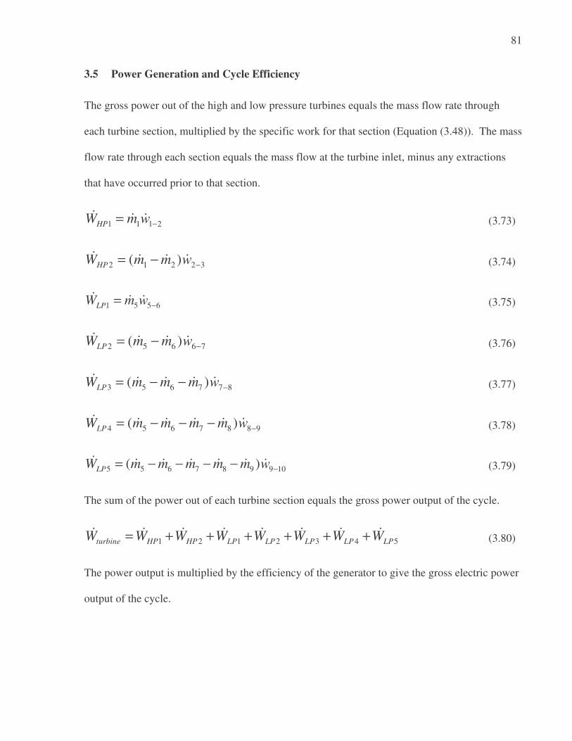
81

3.5 Power Generation and Cycle Efficiency

The gross power out of the high and low pressure turbines equals the mass flow rate through

each turbine section, multiplied by the specific work for that section (Equation (3.48)). The mass

flow rate through each section equals the mass flow at the turbine inlet, minus any extractions

that have occurred prior to that section.

1 1 1 2HPW m w −=� � � (3.73)

2 1 2 2 3( )HPW m m w −= −� � � � (3.74)

1 5 5 6LPW m w −=� � � (3.75)

2 5 6 6 7( )LPW m m w −= −� � � � (3.76)

3 5 6 7 7 8( )LPW m m m w −= − −� � � � � (3.77)

4 5 6 7 8 8 9( )LPW m m m m w −= − − −� � � � � � (3.78)

5 5 6 7 8 9 9 10( )LPW m m m m m w −= − − − −� � � � � � � (3.79)

The sum of the power out of each turbine section equals the gross power output of the cycle.

1 2 1 2 3 4 5turbine HP HP LP LP LP LP LPW W W W W W W W= + + + + + +� � � � � � � � (3.80)

The power output is multiplied by the efficiency of the generator to give the gross electric power

output of the cycle.

82

e turbine generatorW W η= ⋅� � (3.81)

The generator efficiency is a function of the fraction of full load at which the plant operates.

Figure 3.15 shows the efficiency of the generator as a function of load (turbine power over rated

turbine power = 36 [MW] for SEGS VI).

Figure 3.15. Generator efficiency as a function of load, for a power factor of 1.00

(Source: adapted from SEGS VI Engineering Handbook, 1986)

Heat addition to the cycle is provided through the HTF – steam superheater, boiler, preheater,

and reheater. The total heat addition to the cycle equals the sum of the heat transfer through

these heat exchangers.

added superheater steamgenerator preheater reheaterQ Q Q Q Q= + + +� � � � � (3.82)

83

Gross cycle efficiency is the ratio of the gross electric power output to the total heat addition.

,e

cycle gross

added

W

Qη =

�

� (3.83)

Parasitic work from the comprehensive model will include heat transfer fluid pumps, pumps at

the condenser outlet, pumps at the deaerator outlet, and cooling tower/condenser water pumps, as

well as cooling tower fans. In the power cycle model, only the condenser and deaerator pump

parasitics can be approximated. Parasitic work of the condenser pump and the deaerator pump

equals the mass flow rate through each pump multiplied by the specific work of the pump.

12 12 13CPW m w −= ⋅� � � (3.84)

17 17 18DPW m w −= ⋅� � � (3.85)

where CPW� is condenser pump power and DPW� is deaerator pump power. Parasitics for the heat

transfer fluid pumps and cooling tower fans are calculated in the solar field and cooling tower

models, respectively.

Finally, the temperature of the heat transfer fluid returning to the solar field is calculated by an

energy balance over the mixture of the HTF exiting the preheater and the HTF exiting the

reheater. The returning enthalpy of the HTF is the weighted average of the HTF enthalpy exiting

the preheater and reheater.

, , , ,

, ,( )

preheater out preheater out reheater out reheater out

tofield

preheater out reheater out

m h m hh

m m

+=

+

� �

� � (3.86)

84

3.6 Linear Regression Power Cycle Model

The power cycle has been implemented in EES, a simultaneous equation solving software

program (EES, 2005). Property data are taken from EES property functions. The power cycle is

driven by the following three inputs:

1. mass flow rate of the heat transfer fluid;

2. temperature of the HTF at the inlet of the HTF – steam heat exchanger train;

3. turbine exhaust pressure (equal to the condensing pressure)

A linear regression equation can be derived to express the gross electricity output from the power

cycle and the HTF temperature returning to the solar field as a function of these three inputs. A

function of the following form is derived for the gross power output:

2 2

0 1 2 3 4 5 6 7 8grossW a a m a m a P a T a T a m P a m T a P T= + ⋅ + ⋅ + ⋅ + ⋅ + ⋅ + ⋅ ⋅ + ⋅ ⋅ + ⋅ ⋅� � � � � (3.87)

where

grossW� = gross power output from the turbine-generator [MW]

mi

= mass flow rate of HTF [kg/s]

T = temperature of HTF entering HTF – steam heat exchanger train [°C]

P = condensing pressure (pressure of turbine exhaust) [bar]

The following functional form is derived for the HTF temperature returning to the solar field:

2 2

0 1 2 3 4 5tofieldT b b m b m b T b T b m T= + ⋅ + ⋅ + ⋅ + ⋅ + ⋅ ⋅� � � (3.88)

85

where Ttofield is the temperature of the HTF returning to the solar field [°C], and T and m� are as

defined for Equation (3.87) above. Note that in Equation (3.88), the temperature of the HTF

returning to the solar field does not prove to be a significant function of the condensing pressure.

Coefficients for Equation (3.87) and Equation (3.88) are provided in Table 3.3. The linear

regression model is valid for condensing pressures from 0.03 – 1.5 [bar], HTF mass flow rates

from 150 – 500 [kg/s], and solar field outlet temperatures from 250 – 400 [C].

Table 3.3. Coefficients for Equations (3.87) and (3.88)

Coefficient Value Std. Deviation Coefficient Value Std. Deviation

a0 +4.800749E+01 5.888080E-01 b0 -8.50750675E+00 5.508464E-01

a1 -7.447251E-02 1.147754E-03 b1 +7.16221364E-02 1.181532E-03

a2 -4.850291E-05 1.231476E-06 b2 -2.55926225E-04 1.382325E-06

a3 +2.541367E+01 3.537079E+00 b3 +1.01419428E+00 2.969144E-03

a4 -3.353077E-01 2.777871E-03 b4 -1.25871784E-03 4.331759E-06

a5 + 6.032502E-04 3.859045E-06 b5 +6.70025120E-04 2.2858951E-06

a6 -2.142849E-02 4.975414E-03

a7 +4.322630E-04 2.036491E-06

a8 -1.019810E-01 9.219628E-03

Figure 3.16 shows gross power output from the turbine as a function of HTF mass flow rate, at

various lines of constant temperature, for a condensing pressure of 0.08 [bar].

86

Figure 3.16. Electricity output (gross) vs HTF mass flow, at various HTF temperatures entering the power

cycle. Condensing pressure = 0.08 [bar].

It should be noted that HTF mass flow rate and temperature are not independent of one another.

When the solar field model and power cycle model are linked to simulate the entire system, the

linked system will converge on a solar field inlet temperature and outlet temperature for a given

HTF mass flow rate through the field.

3.7 Conclusions

The model used to calculate the outlet temperature of the solar field is discussed in Chapter 2.

The model for the Rankine steam power cycle is described in Chapter 3. A model for the

expansion vessel between the solar field and the power cycle is required to compensate for the

87

thermal capacitance of the heat transfer fluid. Models for the steam condenser and cooling

towers are also required to predict the condensing pressure of the steam. Mathematical

descriptions of the expansion vessel model, the condenser model, and the cooling tower model

are presented in Chapter 4.

88

4 Balance of System Models

4.1 Introduction

Figure 4.1 shows the information flow diagram for all components used in simulation of the

comprehensive solar field / power cycle system.

Figure 4.1. Diagram of inputs and outputs for all components in comprehensive model simulation.

Tfield,outlet

Tfield,inlet

DNI

HTFV� Solar Field

Tambient

Power Cycle

Condenser

Cooling Tower

Storage Tank

HTFm�

HTFm�

Ttank

electricW�

exhaustm�

hexhaust

Pcondense

TCW,2

TCW,1

coolwaterm�

airV�

Tambient

Twetbulb

89

The solar field and power cycle models have been described in Chapters 2 and 3, respectively.

Mathematical descriptions of the storage tank, condenser, and cooling tower models are provided

in the remainder of this chapter.

4.2 Storage Tank

The solar field model does not include thermal capacitance effects; consequently, a storage tank

has been implemented into the TRNSYS model to account for the thermal capacitance of the

heat transfer fluid in the solar field and the expansion vessel. The storage tank is located

between the solar field and the plant’s heat exchanger train. Figure 4.2 shows the information

flow diagram for the storage tank.

The storage tank is modeled with standard TRNSYS component Type 4a (TRNSYS, 2005). The

heat transfer fluid circulating through a solar field in a SEGS plant has considerable thermal

capacitance. During normal operation throughout the day, the field and plant run at a quasi-

steady condition, and the thermal capacitance effects of the solar field heat transfer fluid become

less important. At nighttime, the heat transfer fluid circulating pumps continue to operate (at a

significantly reduced flow) to avoid thermal shocking the collectors during the subsequent day’s

start-up. At night, the heat transfer fluid can experience a significant drop in temperature due to

ambient losses.

90

Figure 4.2. Information flow diagram for the storage tank.

The governing equation behind the storage tank, from an energy balance over the tank, is

( ) ( )tank tank HTF HTF in out loss env in

dTM C m c T T UA T T

dt⋅ = ⋅ − + −� (4.1)

where

Mtank = mass of heat transfer fluid in the tank [kg]

Ctank = heat capacity of the heat transfer fluid in the tank [kJ/kg-K]

cHTF = specific heat of the heat transfer fluid [kJ/kg-K]

UAloss = loss coefficient from the tank [kW/K]

Tin = temperature of the HTF entering the tank [C]

Tout = temperature of the HTF leaving the tank [C]

Tenv = temperature of ambient air surrounding the tank [C]

dT/dt = change in average temperature of the storage tank with time [C/hr]

HTFm� = mass flow rate of HTF [kg/hr]

It is assumed that the mass of fluid in the tank is constant. The storage tank is sized to provide

an equivalent mass as the heat transfer fluid residing in the solar field and expansion vessel. The

mass of the heat transfer fluid in the tank is evaluated from the volume of the HCE receiver tubes

Tank outlet temperature

Solar field outlet temperature Solar field mass flow Ambient air temperature

Parameters Ctank

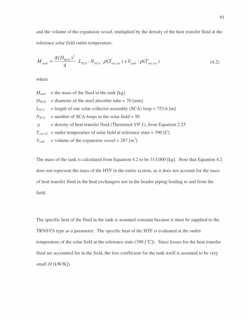
91

and the volume of the expansion vessel, multiplied by the density of the heat transfer fluid at the

reference solar field outlet temperature:

2

, ,

( )( ) ( )

4HCE

tank SCA SCA out ref tank out ref

DM L N T V T

πρ ρ= ⋅ ⋅ ⋅ + ⋅ (4.2)

where

Mtank = the mass of the fluid in the tank [kg]

DHCE = diameter of the steel absorber tube = 70 [mm]

LSCA = length of one solar collector assembly (SCA) loop = 753.6 [m]

NSCA = number of SCA loops in the solar field = 50

ρ = density of heat transfer fluid (Therminol VP-1), from Equation 2.25

Tout,ref = outlet temperature of solar field at reference state = 390 [C]

Vtank = volume of the expansion vessel = 287 [m3]

The mass of the tank is calculated from Equation 4.2 to be 313,000 [kg]. Note that Equation 4.2

does not represent the mass of the HTF in the entire system, as it does not account for the mass

of heat transfer fluid in the heat exchangers nor in the header piping leading to and from the

field.

The specific heat of the fluid in the tank is assumed constant because it must be supplied to the

TRNSYS type as a parameter. The specific heat of the HTF is evaluated at the outlet

temperature of the solar field at the reference state (390 [°C]). Since losses for the heat transfer

fluid are accounted for in the field, the loss coefficient for the tank itself is assumed to be very

small (0 [kW/K]).

92

4.3 Water-Cooled Condenser

Saturated steam vapor exhaust from the low pressure turbine is condensed to saturated liquid

using a shell-and-tube condenser. Condenser water circulates on the tube side of the condenser

while steam condenses on the shell side. Figure 4.3 shows the flow diagram for the cooling

water condenser.

Figure 4.3. Information flow diagram for the cooling water condenser.

The water-cooled condenser model predicts the condensing pressure, given the inlet steam mass

flow rate, entering steam enthalpy, condenser water flow rate, condenser water supply

temperature, and heat exchanger UA. The reference UA for the condenser was calculated to be

3500 [kW/K] from an energy balance over the condenser, using condensing pressure and inlet

and outlet cooling water temperature from the plant data (see calculations in Appendix A). The

UA of the condenser at part-load conditions is a function of the UA at rated power and the ratio

of the condenser water flow rate to the design condenser water flow rate raised to the 0.8 power

(see derivation of UA and mass flow rate dependence in Chapter 3.4):

,steam inm� hsteam coolingwaterm� Tcoolwater,in

Tcoolwater,out Pcondense

Parameters:

UAcondenser,ref

,coolwater refm�

93

0.8

,

,

condensercondenser condenser ref

condenser ref

mUA UA

m

=

�

� (4.3)

The UA of the condenser determines the number of transfer units (NTU) and effectiveness of the

condenser:

condensercondenser

condenser condenser

UANTU

m c=

⋅� (4.4)

1 exp( )condenser condenserNTUε = − − (4.5)

The specific heat of the condenser water, ccondenser , is assumed constant at 4.18 [kJ/kg-K].

The effectiveness of the condenser is the ratio of the heat transfer between condensing steam and

cooling water to the maximum heat transfer possible between these streams at their respective

inlet conditions:

,max

condensercondenser

condenser

Q

Qε =

�

� (4.6)

where

, ,( )condenser steam steam in steam outQ m h h= −� � (4.7)

,max ,( )condenser condenser condenser steam condenser inQ m c T T= ⋅ −� � (4.8)

94

The temperature and pressure of the condensing steam are assumed to be constant throughout the

condenser. The outlet enthalpy of the steam is assumed to be saturated liquid at the condensing

temperature of the steam:

, ( , 0)steam out steamh h T x= = (4.9)

The mass flow rate of exhaust steam, the exhaust steam inlet enthalpy, and the cooling water

inlet temperature are all provided as inputs to the component. Simultaneous solution of

Equations (4.6) through (4.9) determines the saturated condensing temperature of the steam. The

condensing pressure is the pressure corresponding to the saturation temperature of the

condensing steam.

( )condense SAT condenseP P T= (4.10)

The exit temperature of the cooling water is determined from the heat transfer between streams,

assuming constant specific heat for the condenser water:

, ,( )condenser condenser condenser condenser out condenser inQ m c T T= ⋅ −� � (4.11)

The reference parasitic power requirement for the cooling tower is listed at 0.91 [MW], at a

reference condenser water flow rate of 22,000 [gal/min] (Kearney et al, 1988). It is assumed that

this power includes both the four parallel condenser water pumps and the twin two-speed cooling

tower fans. The cooling tower fans are each listed at 156 [hp] (0.116 [MW]) at high speed;

therefore, assume that the reference power requirement for the condenser water pumps is 0.68

[MW]. The reference pressure drop over the condenser water circulation loop (including both

line losses and static pressure head) is calculated from the known reference power and flow rate,

assuming a reference efficiency of 0.60:

95

, ,

.

,

condenser ref condenser ref

condenser ref

condenser ref

WP

V

η ⋅∆ =

�

� (4.12)

The pressure drop coefficient is calculated from the determined reference pressure drop and

reference mass flow rate of condenser water (assuming the density of the condenser water is

constant at 1000 [kg/m3]):

,

,

condenser ref

condenser

condenser ref condenser

Pk

V ρ

∆=

⋅� (4.13)

The reference efficiency of the condenser water pumps is adjusted for partial load flow rates

using the same function as for the deaerator pump and condensate pump for the working fluid

(Equation 3.53).

4.4 Cooling Tower

The cooling tower rejects heat from the circulating cooling water by evaporative heat and mass

transfer to ambient air. The condenser water from the plant is pumped to the top of the tower

and distributed over the cooling tower fill, cascading down the fill to the well at the bottom. Air

is drawn through the bottom of the tower and across the fill media, picking up heat and moisture

and cooling the remaining water in the process. Two fans located at the top of the tower propel

the warm, moist air upward to the ambient environment. Approximately 1-2% of the condenser

water is evaporated in the process, while the remaining water is collected in a sump at the bottom

of the tower and returned back to the condenser. Figure 4.4 shows the information flow diagram

for the cooling tower model.

96

Figure 4.4. Information flow diagram for the cooling tower.

The performance of the cooling tower is quantified through an effectiveness relationship. The

effectiveness method used to model the cooling tower is based on the work of Braun et al

(Braun, 1988). For the cooling tower, the heat rejected from the condenser water stream is

defined as the product of effectiveness, the mass flow rate of the air, and the difference between

the inlet air enthalpy and the enthalpy of saturated air at the inlet temperature of the water.

( )rejected a air w,i iQ m ha ha= ε ⋅ ⋅ −� � (4.14)

where hai refers to the enthalpy of air at the ambient temperature, pressure, and relative

humidity, and haw,i refers to the enthalpy of saturated air evaluated at the inlet temperature of the

cooling water:

, , ,( , , 1)w i water in atmha h air water T P φ= + = (4.15)

, ,( , , )i air in atm ambientha h air water T P φ φ= + = (4.16)

Tcoolwater,out

coolwaterm� Tcoolwater,in Tambient Twetbulb airV�

Parameters

c,n (see Equation 4.21)

Atmospheric pressure, Patm

97

The mass flow rate of air is determined from the volumetric flow rate of air and the density of

the ambient air:

air air airm V= ⋅ρ�� (4.17)

For a counterflow cooling tower, the effectiveness of the cooling tower is related to the number

of transfer units (NTU) and the capacitance ratio through the following relationship:

( )( )( )( )

*

* *

1 exp 1

1 exp 1a

NTU m

m NTU m

− − ⋅ −ε =

− ⋅ − ⋅ − (4.18)

where

* air s

cw cw

m Cm

m c

⋅=

⋅

�

� (4.19)

w,i w,o

s

cw,out cw,in

hs hsC

T T

−=

− (4.20)

The saturated air enthalpies, hsw,i and hsw,o , refer to the enthalpy of saturated air at the inlet

water temperature and outlet water temperature, respectively:

, , ,( , , 1)w i water in atmhs h air water T P φ= + = (4.21)

, , ,( , , 1)w o water out atmhs h air water T P φ= + = (4.22)

The number of transfer units (NTU) for the cooling tower is evaluated as a function of the ratio

of the mass flow rate of cooling water flow rate to the mass flow rate of air:

98

1 n

w

a

mNTU c

m

+

=

�

� (4.23)

The coefficients c and n are obtained from a fit to performance data for the cooling tower (see

Chapter 5).

The two cooling tower fans may be operated at one of two speeds, where the higher operating

speed (106 RPM) is twice the lower operating speed (53 RPM). The power rating for each fan at

high speed is 0.116 [MW]. The parasitic power requirement for each fan at the lower operating

speed is calculated from the speed ratio and high speed power rating using the fan laws:

3

,

,

high fan high

low fan low

W

W

ω

ω

=

�

� (4.24)

4.5 Conclusions

The comprehensive system model consists of five components: a solar field component (Chapter

2), a power cycle component (Chapter 3), and components for the storage tank, the exhaust

steam condenser, and the cooling tower (Chapter 4). This chapter completes discussion of the

component models used to simulate the solar field / power cycle system. In the following

chapter, the solar field, power cycle, and condenser/cooling tower model predictions are

compared to measured plant data from the SEGS VI site.

99

5 Model Validation

5.1 Introduction

At the SEGS plants, a number of state variables are field measured for the purpose of providing

feedback on the plant to operations staff. The types of state variables measured include

temperature, pressure, and flow rate at several locations in the solar field, feedwater/steam plant

and heat rejection systems. The monitored data are logged and reported daily through the plant’s

distributed control system (DCS). The data are logged as instantaneous values at 5 minute

intervals during plant periods of operation between 5:00 A.M. and 8:30 P.M (Local Standard

Time). The DCS is configured to automatically generate daily reports of the plant data collected.

These reports are archived at the plants; data from the first year of operation (1987) to date are

available. The logged plant data are used to validate the solar field model, the power cycle

model, and the heat rejection model (condenser and cooling tower).

Data from two separate years (1998 and 2005) were chosen for model validation. Comparison of

measured values and model predictions from these two sets of data spanning several years allows

for analysis of any change in the performance of the system over time. The days chosen for

model validation had to meet the following criteria:

• Solar-only operation (i.e. no supplemental steam production from natural gas firing),

• Mix of summer, winter, and fall/spring days (to represent the range of operating

conditions experienced by the plant through the year),

• Clear days and cloudy days

100

The days chosen for model validation in the 1998 data year are listed below:

• Day 171 (June 20) – clear day, summer

• Day 262 (September 19) – clear day, fall

• Day 348 (December 14) – cloudy day, winter

• Day 350 (December 16) – clear day, winter

The days chosen for model validation in the 2004 – 2005 data years are listed below:

• Day 162 (June 11) (2005) – slightly overcast day, summer

• Day 141 (May 20) (2005) – clear day, spring

• Day 117 (April 27) (2005) – cloudy day, spring

• Day 71 (March 12) (2005) – clear day, spring

• Day 346 (December 12) (2004) – clear day, winter

The temperature, pressure, and flow rate measurements available in the daily reports that were

used in data consistency analysis and/or model validation are listed in Table 5.1.

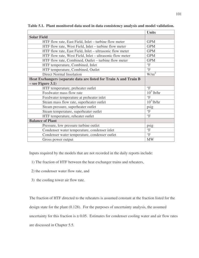
101

Table 5.1. Plant monitored data used in data consistency analysis and model validation.

Inputs required by the models that are not recorded in the daily reports include:

1) The fraction of HTF between the heat exchanger trains and reheaters,

2) the condenser water flow rate, and

3) the cooling tower air flow rate.

The fraction of HTF directed to the reheaters is assumed constant at the fraction listed for the

design state for the plant (0.128). For the purposes of uncertainty analysis, the assumed

uncertainty for this fraction is ± 0.05. Estimates for condenser cooling water and air flow rates

are discussed in Chapter 5.5.

Units

Solar Field

HTF flow rate, East Field, Inlet – turbine flow meter GPM

HTF flow rate, West Field, Inlet – turbine flow meter GPM

HTF flow rate, East Field, Inlet – ultrasonic flow meter GPM

HTF flow rate, West Field, Inlet – ultrasonic flow meter GPM

HTF flow rate, Combined, Outlet – turbine flow meter GPM

HTF temperature, Combined, Inlet °F

HTF temperature, Combined, Outlet °F

Direct Normal Insolation W/m2

Heat Exchangers (separate data are listed for Train A and Train B

– see Figure 3.1)

HTF temperature, preheater outlet °F

Feedwater mass flow rate 103 lb/hr

Feedwater temperature at preheater inlet °F

Steam mass flow rate, superheater outlet 103 lb/hr

Steam pressure, superheater outlet psig

Steam temperature, superheater outlet °F

HTF temperature, reheater outlet °F

Balance of Plant

Pressure, low pressure turbine outlet psig

Condenser water temperature, condenser inlet °F

Condenser water temperature, condenser outlet °F

Gross power output MW

102

5.2 Data Consistency Analysis and Validation

Table 5.2 lists the types of instrumentation used in the SEGS VI solar field and power cycle for

each measurement of interest.

Table 5.2. Instrumentation at SEGS VI.

Measurement Location Instrument Calibration Range* Instrument

Uncertainty

Temperature All temperature readings listed in Table 5.1

Thermocouple, Type K

0 – 800 [°F] (-32 – 427) [°C]

± 2.2 [°C] ��

Pressure Superheater, outlet

Pressure gauge 0 – 2000 [psig] (0 – 138) [bar]

± 5%��

Pressure Low pressure turbine outlet

Pressure gauge 0 – 30 [psig] (0 – 2) [bar]

± 5%��

Volumetric Flow (HTF)

East Field Inlet, West Field Inlet

vortex shedding meter and ultrasonic flow meter

0 – 10,000 [GPM] (turbine) (0 – 0.630) [m3/s] ultrasonic unknown

± 3% (turbine) �� ± 5% (ultrasonic) ��

Volumetric Flow (HTF)

Combined Field Outlet

vortex shedding flow meter

0 – 10,000 [GPM] (0 – 0.630) [m3/s]

± 3%��

Working fluid mass flow (both steam and feedwater)

Feedwater Inlet, Superheater Outlet

orifice plate mass flow meter

0 – 200,000 [lbm/hr] (0 – 25.2) [kg/s]

± 5%��

Direct Normal Insolation (DNI)

Weather station atop SEGS VI – VII control room

Pyrheliometer unknown ± 1%��

*Source: SEGS VI Instrumentation Index, 1987. ��Source: Omega, 2005. ��Source: Ashcroft, 2005. ��Source: Emco, 2005. ��Source: Rosemount, 2005. ��Source: Eppley, 2005.

It is important to note that the uncertainties listed in Table 5.2 are only those specified for the

instrument itself. Any errors in instrument installation, obstruction of instrument probes, or mis-

calibration of the instrument will further compound the uncertainty associated with the

measurement.

103

The data are checked for internal consistency through comparing heat transfer fluid mass flow

rate, solar field inlet temperature, and steam mass flow rate where possible. Each of these

comparisons are discussed in the following sections.

5.2.1 HTF mass flow rate

The mass flow rate of the heat transfer fluid is calculated as the product of the volumetric flow

rate and the density of the fluid at the point of measurement. The HTF mass flow rate is

calculated at the outlet of the solar field and compared to its estimated value at the solar field

inlet, using measurements from both inlet vortex shedding flow meters and inlet ultrasonic flow

meters. The relative error (difference) in HTF mass flow for the vortex shedding and ultrasonic

flow meters is given by Equations (5.1) and (5.2), respectively.

, , , , , , ,

,

, ,

( ) ( ) ( )

( )

HTF out field outlet HTF vortex east HTF vortex west field inlet

HTFflow vortex

HTF out field outlet

V T V V T

V T

⋅ρ − + ⋅ρε =

⋅ρ

� � �

� (5.1)

, , , , , , ,

,

, ,

( ) ( ) ( )

( )

HTF out field outlet HTF sonic east HTF sonic west field inlet

HTFflow sonic

HTF out field outlet

V T V V T

V T

⋅ρ − + ⋅ρε =

⋅ρ

� � �

� (5.2)

Figures 5.1 and 5.2 show the relative difference associated with heat transfer fluid mass flow

rate calculation from Equations 5.1 and 5.2 for two days in 1998 and 2005, respectively.

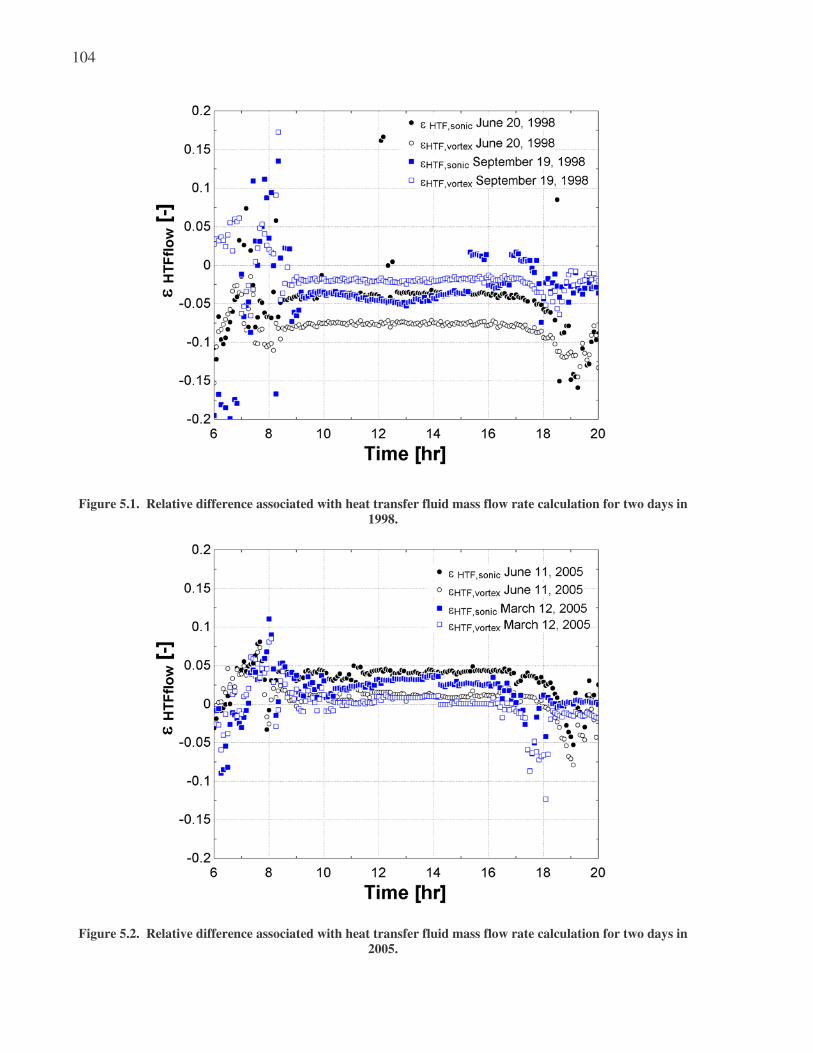
104

Figure 5.1. Relative difference associated with heat transfer fluid mass flow rate calculation for two days in

1998.

Figure 5.2. Relative difference associated with heat transfer fluid mass flow rate calculation for two days in

2005.

105

For the summer day in 1998, the HTF mass flow rate indicated by the vortex meters at the solar

field inlet is about 7.5% lower than the mass flow rate indicated by the vortex meter at the solar

field outlet; for the fall day in 1998 and both days in 2005, the two vortex meters produce mass

flowrates that agree within about 3%. Ultrasonic flow meter predictions in both 1998 and 2005

agree with the vortex outlet meter predictions within 5%. The large scatter in uncertainty seen at

the beginning and end of the measurement period may be attributed to transient system behavior

during start up and shut down.

There is clear systematic difference present in all HTF flow rate measurements in both 1998 and

2005. A systematic difference in the mass flow rate calculations may be attributed to a number

of causes, including the following:

• Mis-calibration of any single instrument;

• Potential difference in cleanliness or probe obstruction between one thermocouple or

flow rate meter and the next;

• Interruption or disturbance in flow read by the ultrasonic meter may be created by the

presence of the vortex shedding flow meter (it is not known which meter is upstream and

which is downstream, nor is the distance between the two instruments known);

• The difference in location between inlet temperature reading and inlet flow rate readings,

as well as between outlet temperature reading and outlet flow rate reading;

• The inlet and outlet temperature thermocouples may be installed at different depths in the

pipe, where a thermocouple inserted closer to the wall of the pipe will read a lower

temperature than a thermocouple inserted closer to the center of the pipe;

106

• The empirical equation for density as a function of temperature may be biased, leading to

more accurate prediction of density at certain temperatures as compared to others. The

equation may also be off if the Therminol VP-1 fluid has degraded with time, or if the

fluid is not pure.

The systematic difference is negative in 1998 (indicating that calculated inlet mass flow rate is

slightly higher than calculated outlet mass flow rate) and positive in 2005; the change in the

direction of the systematic difference indicates the cause of bias is more likely attributed to a

variable that may change with time (such as calibration or probe cleanliness/obstruction) rather

than variables that are not expected to change with time, such as instrument placement.

Fortunately, the systematic difference in the measurements is small and within the accepted

uncertainty of the measurements.

5.2.2 HTF inlet temperature

The measured inlet field temperature is compared to the predicted temperature of the mixed

preheater and reheater outlet streams, using the mass flow rate calculated from the vortex inlet

flow meters and temperature and an assumed splitting fraction of HTF of 0.128 between preheaters

and reheaters for trains A and B.

, , , ,2Tfield inlet field inlet field inletT Tε = − (5.3)

where Tfield,inlet is the measured temperature at the inlet of the solar field, and Tfield,inlet,2 is the

temperature to the solar field calculated from the mixture of HTF streams exiting the preheaters A

and B and reheaters A and B. The temperature of the mixed fluid stream from the two preheaters

and two reheaters is evaluated at the weighted average enthalpy of the four leaving streams:

107

, ,2 , , , ,

, , , ,

(1 ) (1 )( ) ( ) ( )

2 2

( ) ( )2 2

RH RHfield inlet PH out A PH out B

RH RHRH out A RH out B

x xh T h T h T

x xh T h T

− −= + +

+

(5.4)

where

xRH = fraction of HTF directed to the reheaters [-]

TPH,out = temperature of HTF at outlet of preheaters A,B [°C]

TRH,out = temperature of HTF at outlet of reheaters A,B [°C]

Figures 5.3 and 5.4 show the difference in temperature between the measured solar field inlet

temperature and the temperature predicted from mixing the preheater and reheater outlet HTF

streams. In Figure 5.4, the temperature predicted from mixing the preheater and reheater outlet

HTF streams is shown using both the design splitting fraction (0.128) and a fraction of 0.25

(25% of flow is directed to reheaters).

108

Figure 5.3. Difference in measured temperature at the solar field inlet compared to that determined from

mixing of preheater and reheater outlet streams, for two days in 1998.

Figure 5.4. Difference in measured temperature at the solar field inlet as compared to that predicted from

mixing of preheater and reheater outlet streams, for two days in 2005.

109

Temperature agreement for both days in 1998 is excellent, with mixed temperature prediction

differing from solar field inlet temperature by about 1 [°C] on average. Temperature agreement

varies widely throughout the day for both days in 2005. The difference may potentially be

explained in part by a change in the splitting fraction of the heat transfer fluid between the

supeheater-steam generator-preheater train and the reheater (there is no measurement of the HTF

flow rate through individual exchangers that may be used to confirm this observation).

However, even allowing for wide variance in the split of HTF between heat exchanger trains

does not fully reconcile the difference. There is also a clear saddle-shape profile to the relative

differences observed in 2005 in Figure 5.4 that is not seen in the 1998 data in Figure 5.3. Figures

5.5 and 5.6 show the recorded solar field inlet temperature, as well as the outlet HTF

temperatures from the preheaters and reheaters in both Train A and Train B, for data from

September 19, 1998 and data from March 12, 2005.

110

Figure 5.5. Recorded solar field inlet temperature and recorded preheater and reheater HTF outlet

temperatures from September 19, 1998.

111

Figure 5.6. Recorded solar field inlet temperature and recorded preheater and reheater HTF outlet

temperatures from March 12, 2005.

This saddle shape of the relative temperature difference observed in Figure 5.4 may be attributed

to the fact that the recorded solar field inlet temperature in 2005 shows a saddle-shape curve

through the day, while the recorded solar field preheater and reheater outlet temperatures are

fixed at one value through the majority of the day (see Figure 5.6). Also, notice that preheater

and reheater outlet temperatures from Train A and Train B agree fairly well in 1998 (Figure 5.5),

likely indicating that the flow is split evenly between the two trains; there is no such agreement

in outlet temperatures from Train A and Train B in 2005 (Figure 5.6), which may be attributed

either to uneven flow distribution, inaccurate temperature measurements, or, most likely, a

combination of the two. Figures 5.5 and 5.6 are representative of the precision and accuracy of

data in the data files from each respective year. At some time between 1998 and 2005, the data

recorders for the plant reports were programmed such that if the value of the variable being read

112

has not changed appreciably from the previous reading, the new reading is not recorded and the

old reading is carried over in its place. As a result of this recording decision, the mass flow rate

and temperature measurements may show no change at all over long periods of time and exhibit

sharp steps from one time step to the next. The lack of precision in the records is likely the root

cause of the wide temperature variation seen in Figure 5.4.

5.2.3 Steam mass flow rate

The feedwater mass flow rate measured at the preheater inlet (state [20], Figure 3.3) is compared

to the steam mass flow rate measured at the steam superheater outlet (state [1], Figure 3.3).

, ,,

,

( )feedwater A steam Asteamflow A

steam A

m m

m

−ε =

� �

� (5.8)

, ,,

,

( )feedwater B steam B

steamflow Bsteam B

m m

m

−ε =

� �

� (5.9)

Figures 5.7 and 5.8 show the relative difference associated with the steam mass flow rate

measurements for each heat exchanger train for two days in 1998 and 2005, respectively.

113

Figure 5.7. Relative difference associated with steam mass flow rate measurement for two days in 1998.

Figure 5.8. Relative difference associated with steam mass flow rate measurements for two days in 2005.

114

The steam mass flow rates measured at the preheater inlet and superheater outlet consistently

agree within 5% for both heat exchanger train A and heat exchanger train B for all days analyzed

in both 1998 and 2005. There is systematic positive bias in the 2005 data, which may be

attributed to mis-calibration of one or both instruments, obstruction of one or both instruments,

misalignment of one or both instruments in the flow stream, or other sources of systematic

difference as listed in Chapter 5.2.1.

5.2.4 Energy Balances

Finally, an energy balance may be applied over the main heat exchanger trains (superheater,

steam generator, and preheater) to assess whether or not the temperature and flow rate

measurements of the HTF and feedwater streams are physically feasible. The balance of energy

over the main heat exchanger train is calculated as the difference in energy transferred from the

HTF and that transferred to the feedwater/steam, expressed as a fraction of the energy transfer

from the HTF:

HTF steamEnergyBalance

HTF

Q Q

Q

−ε =

� �

� (5.10)

where

, , , , ,

, , , , ,

(1 )( ) ( ) ( )

2

(1 )( ) ( ) ( )

2

RHHTF in vortex field inlet field outlet PH out A

RHin vortex field inlet field outlet PH out B

xQ V T h T h T

xV T h T h T

− = ⋅ ⋅ρ − +

− ⋅ ⋅ρ −

� �

�

(5.11)

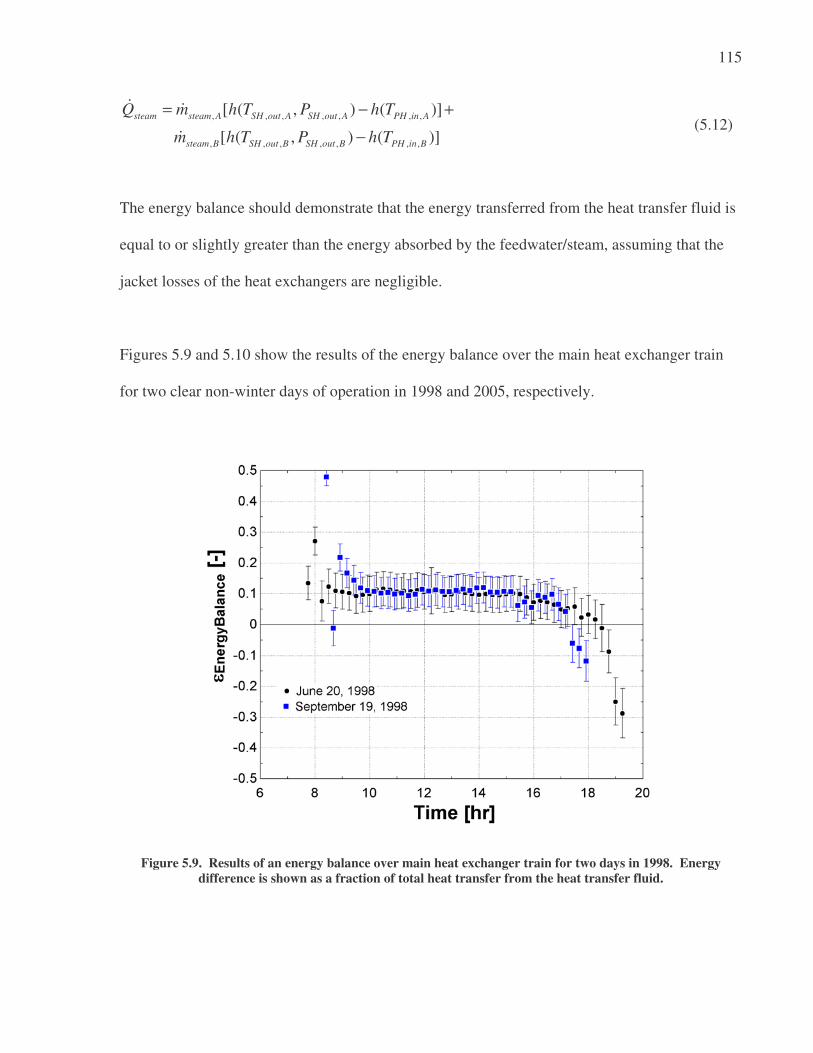
115

, , , , , , ,

, , , , , , ,

[ ( , ) ( )]

[ ( , ) ( )]

steam steam A SH out A SH out A PH in A

steam B SH out B SH out B PH in B

Q m h T P h T

m h T P h T

= − +

−

� �

� (5.12)

The energy balance should demonstrate that the energy transferred from the heat transfer fluid is

equal to or slightly greater than the energy absorbed by the feedwater/steam, assuming that the

jacket losses of the heat exchangers are negligible.

Figures 5.9 and 5.10 show the results of the energy balance over the main heat exchanger train

for two clear non-winter days of operation in 1998 and 2005, respectively.

Figure 5.9. Results of an energy balance over main heat exchanger train for two days in 1998. Energy

difference is shown as a fraction of total heat transfer from the heat transfer fluid.

116

Figure 5.10. Results of an energy balance over main heat exchanger train for two days in 2005. Energy

difference is shown as a fraction of total heat transfer from the heat transfer fluid.

The energy balances over the main heat exchanger train in both 1998 and 2005 show that

calculated energy transfer from the heat transfer fluid is consistently higher than the energy

transfer to the feedwater/steam. According to the calculations, roughly 10% of the energy

transfer from the heat transfer fluid is transferred to the surroundings, depending on the day and

year. The uncertainties in the energy balance, due to the propagated uncertainties associated

with the temperature, pressure, and flow rate readings as listed in Table 5.2., are shown with

error bars in Figures 5.9 and 5.10 to be about ± 5%. Because the error bars do not include a zero

relative energy balance, instrument uncertainty alone is not sufficient to explain the differences.

The relative energy of the heat transfer fluid stream is systematically higher than the steam-side;

therefore, an unaccounted for loss on the steam side could explanation the difference shown in

Figures 5.9 – 5.10. Energy transfer through the heat exchanger jacket to the surroundings seems

117

likely, based on this observation. The difference in calculated energy transfer could also be

attributed to a measurement error of steam flow, HTF flow, or inlet or outlet temperatures that is

greater than the uncertainty used for the measurements. However, many of the data

measurements used in calculating the energy balances have been checked for internal

consistency. Attributing the energy misbalance to instrumental error would require that not one,

but several instrumental readings be in error. For example, if the steam flow rate measurement is

10% too low, then the feedwater flow would also have to be 10% too low.

5.3 Solar Field Model Validation

Direct normal radiation measurements for the days in 1998 and 2005 used to validate the solar

field model are shown in Figures 5.11 and 5.12, respectively.

118

Figure 5.11. Direct normal insolation (DNI) measurements used for 1998 solar field model validation.

Figure 5.12. Direct normal insolation (DNI) measurements for 2005 model validation.

119

The solar field model is validated using direct normal insolation, ambient temperature, solar field

inlet temperature, and solar field volumetric flow rate data from the plant records. The mass

flow rate of heat transfer fluid is calculated from the sum of the volumetric flow rates as

measured by the turbine flow meter to the east and west solar fields, multiplied by the density of

the heat transfer fluid at the measured solar field inlet temperature. The solar field outlet

temperature predicted by the model is compared to the observed outlet temperature as recorded

in the plant data.

Figures 5.13 through 5.20 show measured and predicted outlet temperatures and rates of heat

gain and heat loss from the solar field for four days in 1998, using calculations for solar field

outlet temperature, heat transfer to HTF, and receiver heat loss as detailed in Chapter 2. The

figures show the energy that is absorbed by the receiver tubes ( absorbedQ� ), as well as the receiver

and piping heat losses (Receiver heat loss and piping heat loss, respectively) and the energy that

is absorbed by the heat transfer fluid after thermal losses from the receiver and piping losses

have been accounted for ( retainedQ� ). All energy rates shown in the figures are normalized on a

per unit solar field aperture area basis, so their units are [W/m2]. The uncertainty of the solar

field outlet temperature is determined by propagating the uncertainties of the solar field inlet

temperature, HTF turbine flow rate, and direct normal insolation listed in Table 5.2. An

estimated uncertainty of ±0.01 (absolute) is applied to both the mirror cleanliness factor and the

receiver tube cleanliness factor, to represent the uncertainty in the collector field efficiency and

HCE receiver tube efficiency calculations (see Chapter 2). It is assumed that all physical

dimensions of the solar field are well known.

120

Figure 5.13. Rates of heat absorption and heat loss from the solar field for June 20, 1998. The measured

direct normal insolation is provided for reference.

Figure 5.14. Measured and predicted outlet temperatures from the solar field for June 20, 1998.

121

Figure 5.15. Rates of heat absorption and heat loss from the solar field for September 19, 1998. The

measured direct normal insolation is provided for reference.

Figure 5.16. Measured and predicted outlet temperatures from the solar field for September 19, 1998.

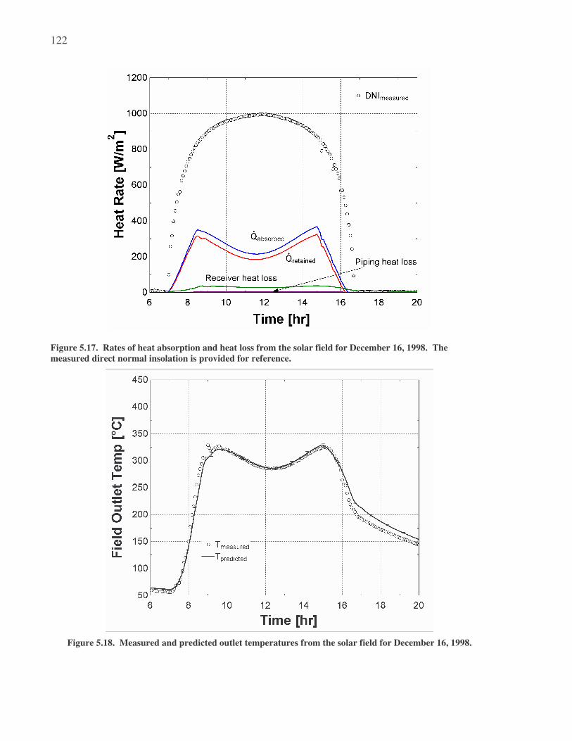
122

Figure 5.17. Rates of heat absorption and heat loss from the solar field for December 16, 1998. The


Figure 5.18. Measured and predicted outlet temperatures from the solar field for December 16, 1998.

123




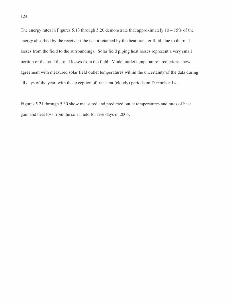
124

The energy rates in Figures 5.13 through 5.20 demonstrate that approximately 10 – 15% of the

energy absorbed by the receiver tube is not retained by the heat transfer fluid, due to thermal

losses from the field to the surroundings. Solar field piping heat losses represent a very small

portion of the total thermal losses from the field. Model outlet temperature predictions show

agreement with measured solar field outlet temperatures within the uncertainty of the data during

all days of the year, with the exception of transient (cloudy) periods on December 14.

Figures 5.21 through 5.30 show measured and predicted outlet temperatures and rates of heat

gain and heat loss from the solar field for five days in 2005.

125

Figure 5.21. Rates of heat absorption and heat loss from the solar field for June 11, 2005. The measured


Figure 5.22. Measured and predicted outlet temperatures from the solar field for June 11, 2005.

126

Figure 5.23. Rates of heat absorption and heat loss from the solar field for May 20, 2005. The measured


Figure 5.24. Measured and predicted outlet temperatures from the solar field for May 20, 2005.

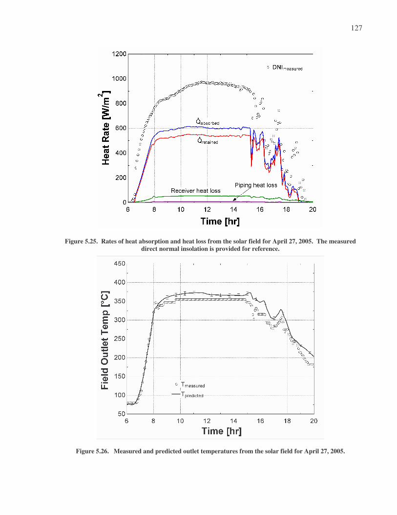
127

Figure 5.25. Rates of heat absorption and heat loss from the solar field for April 27, 2005. The measured


Figure 5.26. Measured and predicted outlet temperatures from the solar field for April 27, 2005.

128

Figure 5.27. Rates of heat absorption and heat loss from the solar field for March 12, 2005. The measured


Figure 5.28. Measured and predicted outlet temperatures from the solar field for March 12, 2005.

129




130

The outlet temperature predictions from the model agree with the measured data on all days to

within 8 – 9 [°C]. For the December and March days simulated, where the outlet temperature of

the solar field is relatively low, the predicted outlet temperatures run slightly higher than

measured temperatures (2 – 4 [°C]). For the April, May, and June days, when the outlet

temperature of the field is high, solar field outlet temperature predictions from the model are

consistently and significantly higher than measured solar field outlet temperatures by 8 – 9 [°C];

the difference is not explained by the uncertainty of the model predictions, as seen by the lack of

overlap between the error bars on the model predicted data with the actual observed data. In the

above calculations, it is assumed that all of the receivers have their vacuums intact. The

discrepancy in outlet temperatures in 2005 might be attributed, in part, to compromise of the

vacuum annulus of the solar field receivers. Modeling of performance losses from the solar field

and solar field/power cycle system as a result of this trend is discussed further in Chapter 6.

The difference between outlet temperature model predictions and measured field outlet

temperatures is quantified by the use of a statistical measure, the average root mean square

difference (RMSD):

2

, ,

1

( )n

measured i predicted i

i

x x

RMSDn

=

−

=∑

(5.13)

RMSD values for the solar field outlet temperatures predicted through mid-day operation (10

a.m. through 4 p.m.) are shown for each day simulated in 1998 and 2005 in Table 5.3.

131

Table 5.3. RMSD through mid-day operation for each simulated day

Day/Year RMSD

June 20, 1998 1.96 [°C]

September 19, 1998 1.07 [°C]

December 14, 1998 10.9 [°C]

December 16, 1998 2.65 [°C]

June 11, 2005 12.1 [°C]

May 20, 2005 9.91 [°C]

April 27, 2005 18.6 [°C]

March 12, 2005 5.68 [°C]

December 12, 2004 6.44 [°C]

The standard deviation during clear days in 1998 lies in a range from 1 – 3 [°C], with a standard

deviation on the cloudy day of almost 11 [°C]. The standard deviation in 2005 lies in a range

from about 10 – 12 [°C] in the late spring/summer and ranges from 5 – 7 [°C] in the early spring

and winter. Standard deviation on the cloudy day modeled in 2005 is just under 19 [°C]. It is

clear from the standard deviations that model agreement with measured data is much closer in

1998 as compared to 2005, especially in the spring and summer months.

The sensitivities of the solar field outlet temperature to each of the input variables and assumed

uncertainty of the mirror and receiver tube cleanliness are shown in Table 5.4. The sensitivities

(% uncertainties) represent the proportion of the propagated uncertainty in solar field outlet

temperature contributed by each variable. The values shown in the table are those calculated at

noon on June 20, 1998.

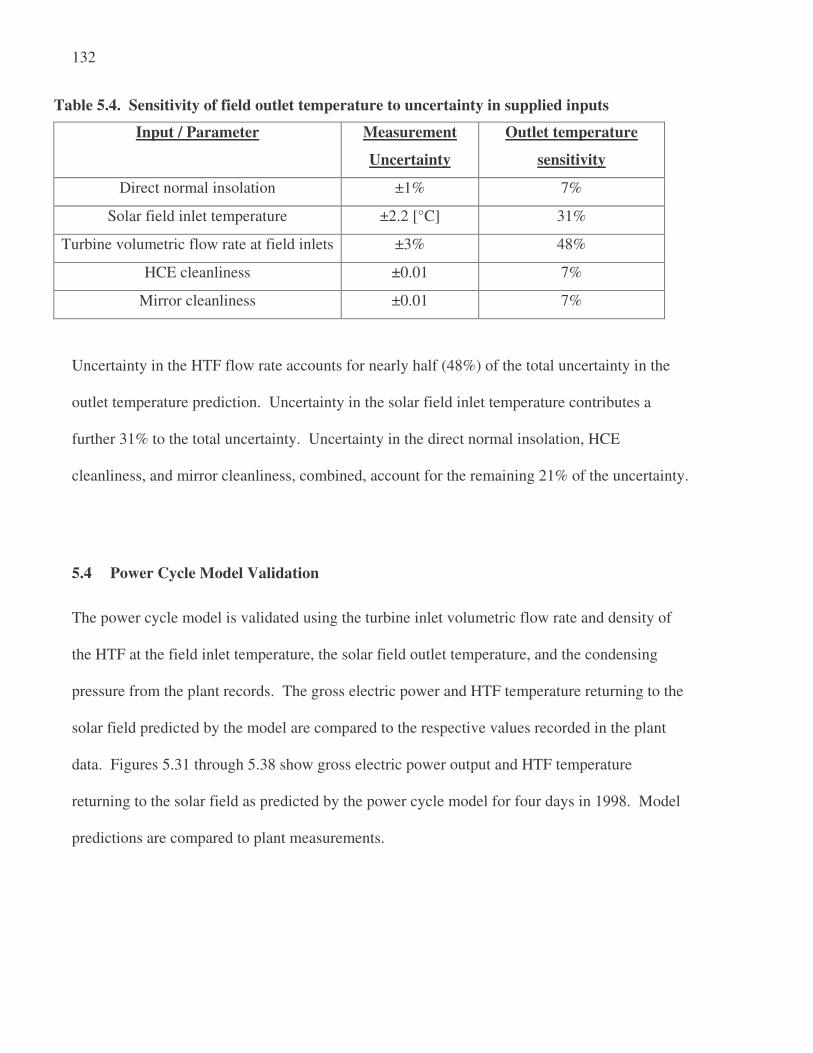
132

Table 5.4. Sensitivity of field outlet temperature to uncertainty in supplied inputs

Input / Parameter Measurement

Uncertainty

Outlet temperature

sensitivity

Direct normal insolation ±1% 7%

Solar field inlet temperature ±2.2 [°C] 31%

Turbine volumetric flow rate at field inlets ±3% 48%

HCE cleanliness ±0.01 7%

Mirror cleanliness ±0.01 7%

Uncertainty in the HTF flow rate accounts for nearly half (48%) of the total uncertainty in the

outlet temperature prediction. Uncertainty in the solar field inlet temperature contributes a

further 31% to the total uncertainty. Uncertainty in the direct normal insolation, HCE

cleanliness, and mirror cleanliness, combined, account for the remaining 21% of the uncertainty.

5.4 Power Cycle Model Validation

The power cycle model is validated using the turbine inlet volumetric flow rate and density of

the HTF at the field inlet temperature, the solar field outlet temperature, and the condensing

pressure from the plant records. The gross electric power and HTF temperature returning to the

solar field predicted by the model are compared to the respective values recorded in the plant

data. Figures 5.31 through 5.38 show gross electric power output and HTF temperature

returning to the solar field as predicted by the power cycle model for four days in 1998. Model

predictions are compared to plant measurements.

133

Figure 5.31. Gross power predicted by the power cycle model as compared to measured gross electric power

for June 20, 1998.

Figure 5.32. HTF temperature returning to the solar field, predicted by the power cycle model, as compared

to measured solar field inlet temperature, for June 20, 1998.

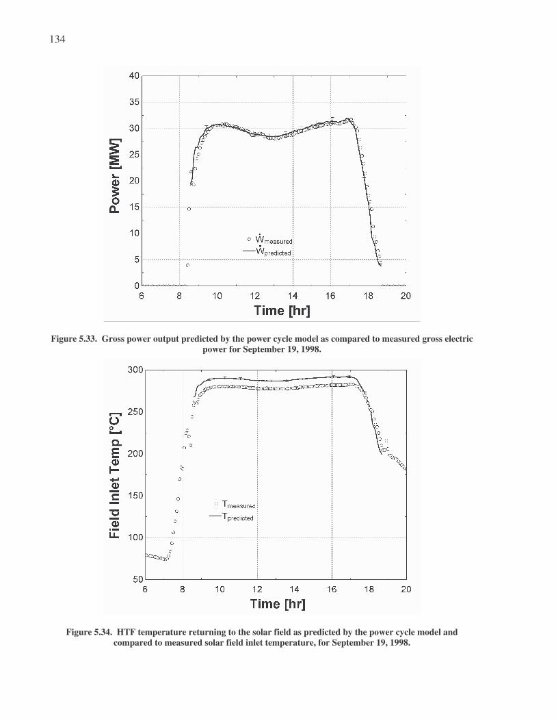
134

Figure 5.33. Gross power output predicted by the power cycle model as compared to measured gross electric

power for September 19, 1998.

Figure 5.34. HTF temperature returning to the solar field as predicted by the power cycle model and

compared to measured solar field inlet temperature, for September 19, 1998.

135


power for December 16, 1998.


compared to measured solar field inlet temperature, for December 16, 1998.

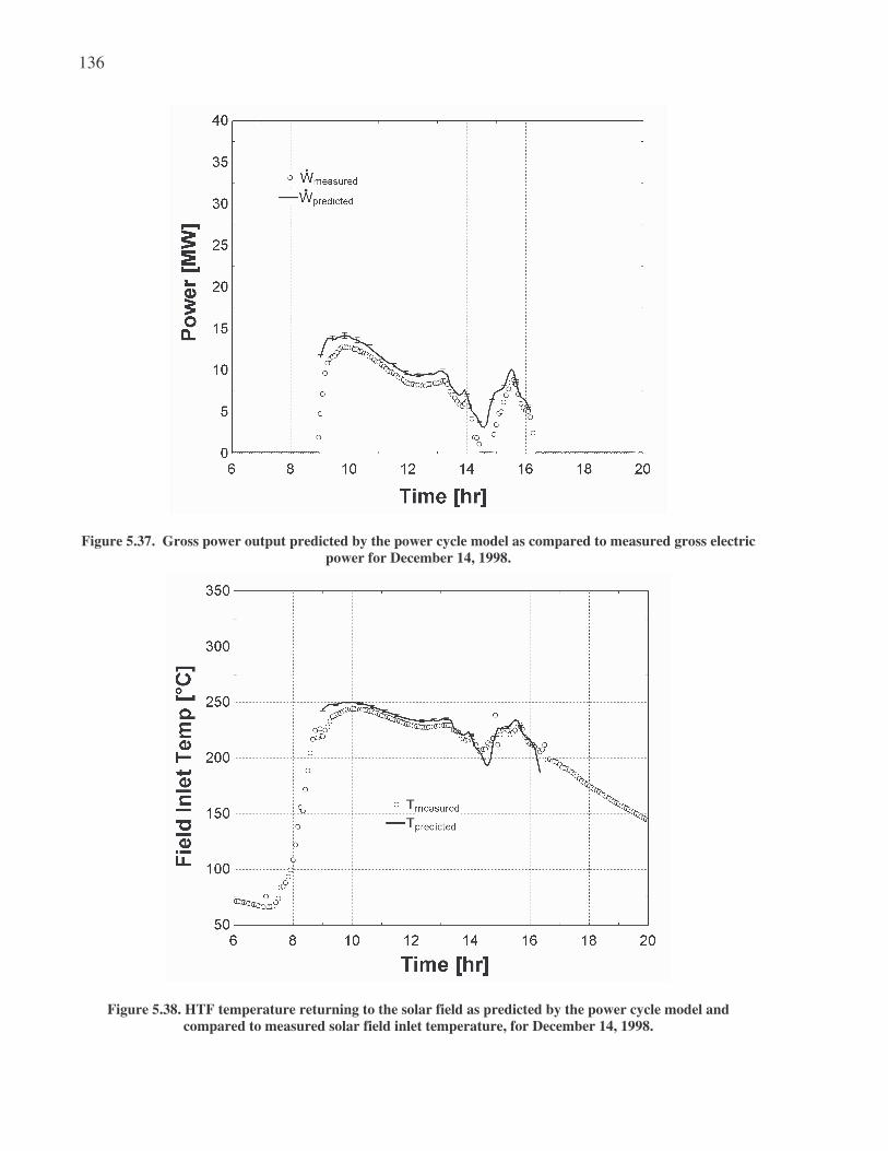
136





137

Gross electric power predicted by the model shows agreement within the uncertainty (+/- 1%) on

Day 171 and Day 262, and is about 10% higher than measured power, at most, on Days 348 and

350. The high gross electricity predictions on the winter days may likely be attributed to

inaccurate estimates of the partial load efficiency of the turbine stages.

The outlet temperature predicted by the model is 7 – 10 [°C] higher than measured solar field

inlet temperatures in all scenarios for 1998. This temperature difference is not explained by the

propagated uncertainties of the measurements of either the solar field inlet temperature or the

parameters (solar field flow rate, outlet temperature, condensing pressure, and reheat fraction)

used to run the simulation. The high temperatures must be attributed to thermal losses from the

heat exchanger equipment not included in the model.

Figures 5.39 through 5.48 show gross electric power output and HTF temperature returning to

the solar field as predicted by the power cycle model for a winter day in 2004 and four days in

2005. Model predictions are compared to plant measurements.

138


power for June 11, 2005.

Figure 5.40. HTF temperature returning to solar field predicted by the power cycle model as compared to

measured solar field inlet temperature for June 11, 2005.

139

Figure 5.41 Gross power output predicted by the power cycle model as compared to measured gross electric

power for May 20, 2005.


compared to measured solar field inlet temperature, for May 20, 2005.

140


power for April 27, 2005.


compared to measured solar field inlet temperature, for April 27, 2005.

141


power for March 12, 2005.


compared to measured solar field inlet temperature, for March 12, 2005.

142





143

The power cycle model generally agrees with the data to within about 1.5 [MW]. The stair-step

shape of the curves is attributed to the solar field outlet temperature, where the measured outlet

temperature trend exhibits a similar shape (see Figures 5.23, 5.25, 5.27, 5.29, and 5.31).

Temperature predictions at the outlet of the heat exchanger train are consistently and

significantly higher than those measured. The difference is not explained by the uncertainty in

the analysis. The difference is likely attributed to thermal losses from the HTF system (heat

exchangers, piping, and HTF pumps) not included in the model.

RMSD values for the gross electric power and solar field inlet temperatures predicted by the

power cycle through mid-day operation (10 a.m. through 4 p.m.) are shown for each day

simulated in 1998 and 2005 in Table 5.5.

Table 5.5. RMSD and average uncertainty values

Day/Year

Power

[MW]

RMSD

Temperature

[°C]

RMSD

June 20, 1998 0.279 10.5

September 19, 1998 0.318 9.54

December 14, 1998 1.85 5.23

December 16, 1998 1.52 6.28

June 11, 2005 0.835 6.65

May 20, 2005 0.795 8.74

April 27, 2005 1.31 8.67

March 12, 2005 1.36 8.55

December 12, 2004 0.835 10.0

144

The sensitivities of the power cycle model outputs to the uncertainty in the HTF temperature,

HTF flow rate, condensing pressure, and fraction of the HTF directed to the reheaters are shown

in Table 5.6. The values shown in the table are those calculated at noon on June 20, 1998.

Table 5.6. Sensitivity analysis for power cycle model as a function of power cycle inputs

Input / Parameter Measurement

Uncertainty

% Uncertainty, Tout % Uncertainty, Power

Solar field outlet

temperature

±2.2 [°C] 8% 25%

Turbine volumetric flow

rate at field inlets

±3% 87% 70%

Condensing pressure ±5% 0% 3%

fraction of HTF directed

to reheaters

±0.05 5% 2%

The largest source of uncertainty in both electric power and HTF heat exchanger outlet

temperature prediction is the HTF flow rate, representing 70% and 87% of the total uncertainty

in the prediction, respectively. The solar field outlet temperature provides the next largest source

of uncertainty in the model predictions. Uncertainty in the condensing pressure and the fraction

of the HTF directed to the reheaters represent relatively small contribution to the total

uncertainty of the model predictions. Notice that the condensing pressure (±5%) has no

significant effect on the HTF temperature at the heat exchanger train outlet.

145

5.5 Condensing Pressure Predictions versus Plant Data

The condensing temperature and pressure of the steam in the power cycle are calculated from a

surface condenser model. Inputs to the model include the entering enthalpy and mass flow rate

of the condensing steam and condenser water. The model returns condensing pressure and

temperature of the cooling water at the condenser outlet.

Plant records include measurements of entering condenser water temperature, leaving condenser

water temperature, and exhaust pressure (at the outlet of the low pressure turbine which is

assumed to be equal to the condensing pressure). The condenser and cooling tower models also

require flow rates for the condenser water and air flow rates through the tower. No data are

available in the plant records regarding the flow rates of these streams or the auxiliary power

consumption for the cooling tower fans and condenser water circulating pumps. The condenser

water flow rate is estimated from an energy balance on the condenser, using the measured

cooling water inlet and outlet temperatures for the condenser, a constant water specific heat of

4.181 [kJ/kg-K], and the heat rejected from the power cycle. Heat rejection is calculated from

the measured condensing pressure and the enthalpy and steam mass flow entering the condenser

component in the power cycle model (see Chapter 3):

( )11 11rejected cw cw cw,out cw,inQ Q m m c T T= − ⋅ = ⋅ ⋅ −� � � � (5.14)

The cooling tower has two cells, each of which is cooled by one 36 [ft] (11 [m]) diameter, 165

HP (123 kW) fan. Each fan can operate at one of two speeds: high speed (106 RPM), and low

speed (53 RPM). On summer days and spring/fall days, the assumption is made that both

cooling tower fans operate throughout the day at high speed; it is assumed that both cooling

146

tower fans operate at low speed throughout the day on the winter days. The volumetric flow rate

of air through one cooling tower fan is estimated by calculating the theoretical air velocity off of

the fan blade. The theoretical maximum air velocity off the fan blade is equal to the vector

component of velocity in the vertical (upwards) direction multiplied by the angular velocity. The

pitch of the fan blades is given in the cooling tower specifications to be 9°. The theoretical

average velocity of air off the fan blade in the vertical direction at the center of the fan blade is

2 sin( )V Rπω θ= (5.15)

where

R = radius, measured from the fan hub to the center of the fan blade ≈ 9 [ft] (3 [m])

θ = pitch of the fan blade = 9 [degrees]

ω = rotational speed of the fan blades = 106 [RPM]

For the given average radius of the fan blade, pitch, and rotational speed, the average velocity of

air through the fans is estimated at 4.75 [m/s]. With a fan cross sectional area of (πD2/4 = 94.5)

[m2], the fan volumetric flow rate at high speed is estimated at 450 [m3/s], for each fan.

Ambient air temperature measurements are provided in the weather data files for the plant.

Atmospheric air pressure is estimated at 1 [atm]. There are no data provided in the plant weather

files representing the relative moisture content of the air; the moisture content of the air is

estimated from hourly dew point measurements taken at the Barstow/Daggett Airport for the

days modeled (National Oceanic and Atmospheric Association, 2005).

147

From the estimated flow rates of the air and cooling water, the weather data, and the cooling

water temperatures at the inlet and outlet of the cooling tower, using Equations (4.10) through

(4.16), the number of transfer units (NTU) for the cooling tower can be predicted at several

points in time throughout the operating day. The number of transfer units is calculated as a

function of the ratio of the cooling water mass flow rate to the air mass flow rate (Braun, 1988):

1n

condenserwater

air

mNTU c

m

+

=

�

� (5.16)

where:

NTU = number of transfer units [-]

c = Y-intercept of log-log plot of NTU versus mass flow ratio [-]

n = slope of log-log plot of NTU versus mass flow ratio [-]

condenserwaterm� = mass flow rate of condenser water [-]

airm� = mass flow rate of air [-]

Figure 5.49 shows the number of transfer units calculated for the cooling tower as a function of

the ratio of cooling water mass flow rate to air mass flow rate. The plot shows NTU values

calculated for a summer day in 2005, a winter day in 2004, and a summer and winter day in

1998.

148

Figure 5.49. Number of transfer units (NTU) calculated for the cooling tower, as a function of measured

cooling water temperatures, weather data, and estimated cooling water and air mass flow rates.

The mass flow ratio generally ranges from 1 to 2, where the mass flow rate of condenser water is

greater than the mass flow rate of air. The coefficients c and n are obtained from a curve fit to

the NTU / mass flow rate calculations shown in Figure 5.49 and are found to be 1.138 and 1.75,

respectively.

Figures 5.50 through 5.57 show temperature predictions of the condenser cooling water at the

inlet and outlet of the steam condenser, as well as the predicted condensing pressure of the

steam, as compared to plant measurements for a summer and winter day in 1998, a summer day

in 2005, and a winter day in 2004.

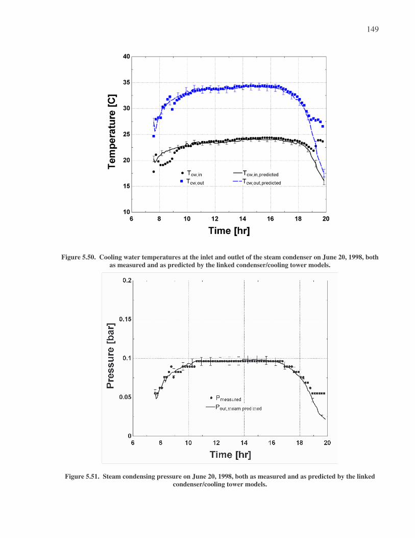
149

Figure 5.50. Cooling water temperatures at the inlet and outlet of the steam condenser on June 20, 1998, both

as measured and as predicted by the linked condenser/cooling tower models.

Figure 5.51. Steam condensing pressure on June 20, 1998, both as measured and as predicted by the linked

condenser/cooling tower models.

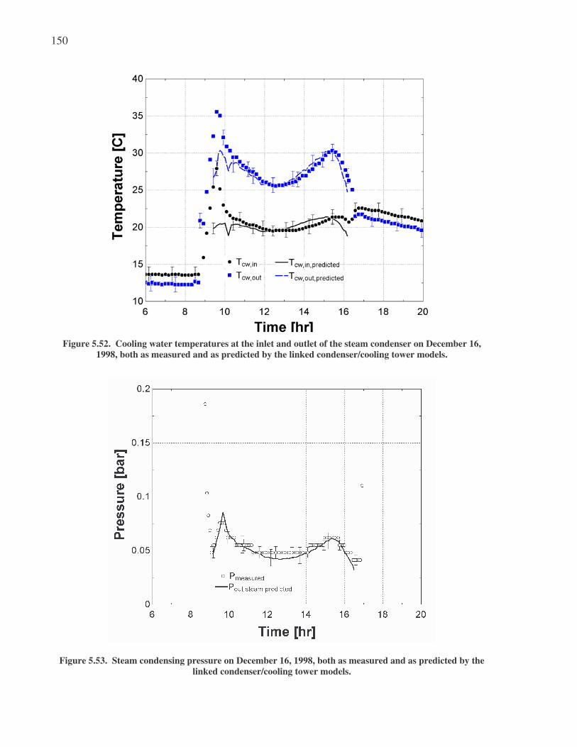
150

Figure 5.52. Cooling water temperatures at the inlet and outlet of the steam condenser on December 16,

1998, both as measured and as predicted by the linked condenser/cooling tower models.

Figure 5.53. Steam condensing pressure on December 16, 1998, both as measured and as predicted by the

linked condenser/cooling tower models.

151

Figure 5.54. Cooling water temperatures at the inlet and outlet of the steam condenser on June 11, 2005, both

as measured and as predicted by the linked condenser/cooling tower models.

Figure 5.55. Steam condensing pressure on June 11, 2005, both as measured and as predicted by the linked

condenser/cooling tower models.

152

Figure 5.56. Cooling water temperatures at the inlet and outlet of the steam condenser on December 12, 2004,

both as measured and as predicted by the linked condenser/cooling tower models.

Figure 5.57. Steam condensing pressure on December 12, 2004, both as measured and as predicted by the

linked condenser/cooling tower models.

153

The entering and leaving condenser water temperatures agree within the uncertainty of the field

measurements for both the summer day and the winter day in 1998. Condensing pressure

predictions in 1998 agree within the uncertainty of the data as well. Predictions for condenser

water temperatures and condensing pressures in 2005 do not match measured data within the

uncertainty of the measurements. This disagreement is likely due in large part to the lack of

reliability in the 2005 recorded data as compared to the 1998 data (see section 5.2).

5.6 System Gross Electric Power Predictions versus Plant Data

The comprehensive model represents the complete solar field/power cycle system, in which the

power cycle, solar field, expansion vessel, condenser, and cooling tower components are all

connected to represent the entire system. The information flow diagram, which shows input and

output connections for all models linked in the solar field/ power cycle combined system, is

provided as Figure 4.1 in Chapter 4. The inputs required to the comprehensive model are:

1) HTF mass flow rate [kg/s] (calculated from inlet volumetric flow rate and density at inlet temperature, both provided in the plant data);

2) direct normal insolation [W/m2] (provided in the plant data);

3) ambient air temperature [C] (provided in the plant data);

4) dew point temperature [C] (from hourly temperatures recorded at Daggett/Barstow airport);

5) cooling water mass flow rate [kg/s] (estimated from energy balance over condenser); and

6) air volumetric flow rate [m3/s] (estimated from rated rotational speed and pitch angle of fan)

154

For all days in both 1998 and 2005, the predicted temperature of the HTF at the outlet of the heat

exchanger train was consistently higher than the measured solar field inlet temperature. A heat

exchanger heat loss calculation is added between the heat exchanger outlet and the solar field

inlet to correct for this observed difference. The rate of heat transfer from the heat exchanger

train to the surroundings is expressed as a function of an overall heat transfer conductance-area

product (UA) for the heat exchanger train and the temperature difference between the HTF at the

heat exchanger outlet and the ambient air:

,( )loss loss HTF HXout ambientQ UA T T= −� (5.17)

where

lossQ� = heat transfer due to thermal losses from the heat exchangers to the surroundings

[kW]

lossUA = UA of heat transfer from heat exchangers to surroundings [kW/K]k

,HTF HXoutT = temperature of HTF at heat exchanger outlet that would be achieved were there

no compensation for thermal losses [°C]

ambientT = temperature of ambient air [°C]

The calculated heat transfer from the HTF to the surroundings is used to calculate the difference

in enthalpy (and thus the difference in temperature) between the HTF outlet temperature without

ambient losses and the HTF outlet temperature with ambient losses:

( ),( ) lossSFinlet HTF HXout

HTF

Qh T h T

m= −

�

� (5.18)

155

From the difference in measured and predicted solar field inlet temperature at noon on June 20,

1998. the heat transfer to the surroundings is found to be 10,900 [kW], and the calculated UA for

the thermal losses is 35 [kW/K].

The uncertainty of the power output predicted by the comprehensive model is a function of the

uncertainty in the measurements of the plant data, as well as the uncertainty of the estimated

condenser water and air flow rates. The air mass flow rate is assumed to have an uncertainty of

±5%; an uncertainty of ±5% is also assumed for the condenser water flow rate. Uncertainty in

the mirror cleanliness and HCE cleanliness performance factor of ±0.02 (absolute) are included

in the uncertainty analysis as well.

Figures 5.58 through 5.65 show gross electric power predictions from the comprehensive model

for four days in 1998 and five days in 2004 – 2005.

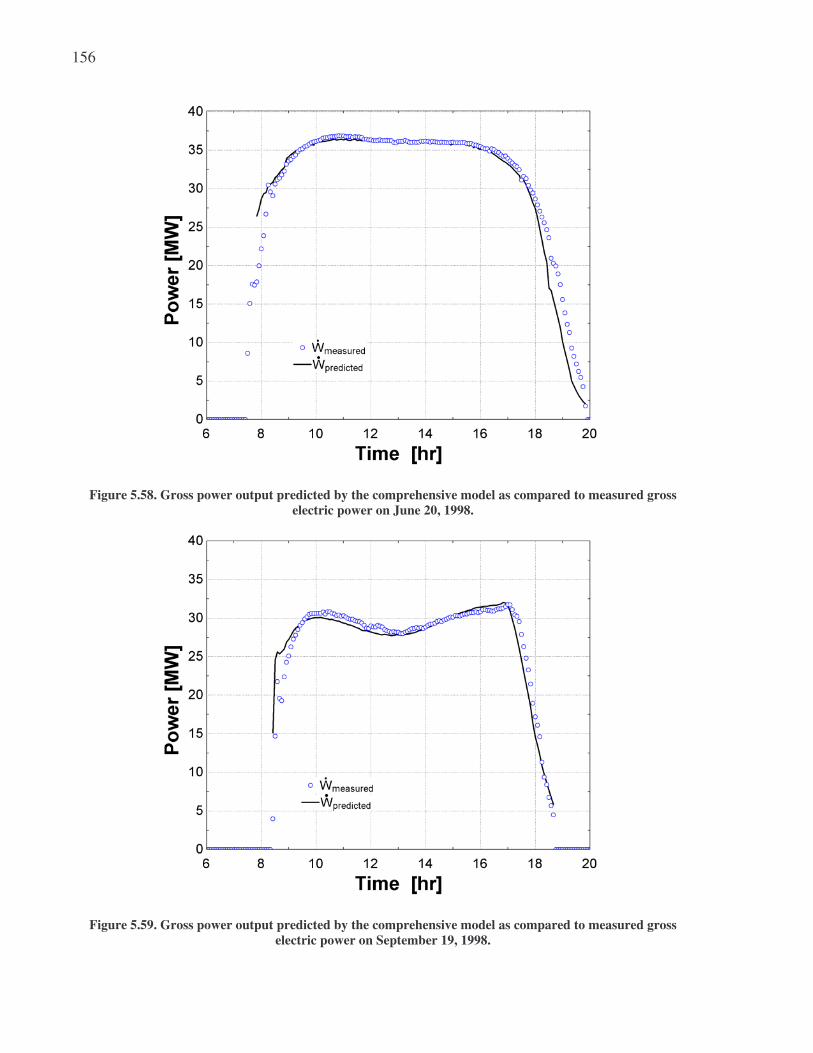
156

Figure 5.58. Gross power output predicted by the comprehensive model as compared to measured gross

electric power on June 20, 1998.


electric power on September 19, 1998.

157


electric power on December 14, 1998.



158


electric power on June 11, 2005.


electric power on May 20, 2005.

159


electric power on April 27, 2005.


electric power on March 12, 2005.

160



Gross power predictions agree with measured gross electric power within the uncertainty of the

measurements for the June and September days modeled in 1998. The difference between

predicted and gross power at the second saddle peak on the clear winter day in 1998 (December

16) is about 1.5 [MW], or 10% of the peak measured gross electric power on that day. Gross

power predictions at the second saddle peak on the winter day in 2004 are also high, by about 1.3

[MW]. Gross power predictions on the April, May, and June days modeled in 2005 are

consistently higher than measured gross electric power by about 4 [MW].

161

5.7 Conclusions

The solar field model shows that higher solar field outlet temperatures were achieved in the

summer and spring/fall days in 1998 than in 2005. The system model also shows that higher

gross electric power production (4 [MW]) was achieved in summer and spring/fall days in 1998

than in 2005. The trend indicates that some loss in performance has occurred in the solar field in

the period between 1998 and 2005. One possibility is that loss of vacuum in the HCE annular

space over the course of several years has contributed to this decline in performance. The effects

of HCE annulus condition on solar field performance and subsequent power production are

covered in Chapter 6.

162

6 Solar Field Performance Analysis

6.1 Introduction

Chapter 5 demonstrated the validity of the solar field model of the SEGS plant. Based on the

input of measured data consisting of the inlet heat transfer fluid (HTF) temperature, HTF flow

rate, direct normal insolation, and ambient air temperature, the predicted solar field outlet

temperatures agreed with measured outlet temperatures within the range of measurement

uncertainty for both the day in September and the day in June in 1998. Without changing any of

the collector field/HCE properties or other performance factors, the same model consistently

over-predicted solar field outlet temperatures for independent days selected during the months of

April, May, and June 2005. Based on the over-prediction, it appears that there has been some

degradation in the performance of the solar field in the period between 1998 and 2005.

Researchers at National Renewable Energy Laboratory (Price, personal communication, 2005)

believe that a significant fraction of the performance loss observed between 1998 and 2005 may

be attributed to compromise of the vacuum annulus in the solar field heat collection elements

(HCEs). The HCEs are composed of an absorber tube surrounded by a glass envelope. To

minimize thermal losses, the annular space between the tube and the envelope is evacuated when

manufactured. Over several years of operation, the potential exists for the vacuum to be

compromised, resulting in ambient air infiltrating the annular space. The introduction of ambient

air in the annular space will increase the thermal losses and, consequently, decrease the energy

collected. Another mechanism that can compromise the annular vacuum is “hydrogen

163

permeation.” Hydrogen from the synthetic heat transfer fluid can dissociate from the fluid and

migrate through the stainless steel absorber tube into the annular space. Because the thermal

conductivity of hydrogen is approximately 6.5 times greater than that of air at 350°C, thermal

losses from the collectors will increase significantly. Performance losses in the solar field as a

result of hydrogen permeation, as well as the resulting diminished electricity production, are the

focus of this chapter.

6.2 Assumptions

It has been estimated that as many as 50% of the collectors in the solar field have been

compromised, in part, by hydrogen permeation (Price, personal communication, 2005). A

program to provide detailed heat transfer analysis of the heat transfer rates through the HCE was

developed by Forristall (2003). Chapter 2 describes the use of Forristall’s HCE design program

to determine thermal losses from the HCE per unit length trough [W/m] as a function of the bulk

HTF temperature and direct normal insolation. Losses are considered for three separate cases:

1. annular space is evacuated at a pressure of 0.0001 [torr], as in its as-manufactured state (base case)

2. ambient air has infiltrated the annular space at atmospheric pressure (760 [torr])

3. hydrogen has infiltrated the annular space at a pressure of (1 [torr])

Assumptions regarding the HTF flow rate, ambient air temperature, and physical dimensions and

surface properties of the HCE elements are reviewed in Chapter 2.

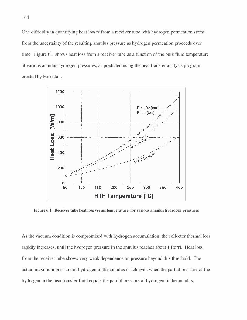
164

One difficulty in quantifying heat losses from a receiver tube with hydrogen permeation stems

from the uncertainty of the resulting annulus pressure as hydrogen permeation proceeds over

time. Figure 6.1 shows heat loss from a receiver tube as a function of the bulk fluid temperature

at various annulus hydrogen pressures, as predicted using the heat transfer analysis program

created by Forristall.

Figure 6.1. Receiver tube heat loss versus temperature, for various annulus hydrogen pressures

As the vacuum condition is compromised with hydrogen accumulation, the collector thermal loss

rapidly increases, until the hydrogen pressure in the annulus reaches about 1 [torr]. Heat loss

from the receiver tube shows very weak dependence on pressure beyond this threshold. The

actual maximum pressure of hydrogen in the annulus is achieved when the partial pressure of the

hydrogen in the heat transfer fluid equals the partial pressure of hydrogen in the annulus;

165

however, since the partial pressure of hydrogen in the heat transfer fluid is not known, this

condition can not be applied as the upper bound on the hydrogen pressure. For the analysis

presented in this chapter, it is assumed that hydrogen permeated tubes have an annulus pressure

of 1 [torr]. This pressure is selected to represent an upper limit on the heat loss from an HCE

with hydrogen in the annulus, as heat loss is a very weak function of pressures at pressures

greater than 1 [torr].

6.3 Change in Solar Field Heat Retention and Outlet Temperature

Outlet temperatures predicted by the solar field model are compared with plant data temperatures

for two cases in 2005, which are referenced using the following terms:

Vacuum Field Case: The solar field consists entirely of glass enveloped heat collection

elements (HCEs) with vacuum in the annulus, as originally designed (base case)

Hydrogen Field Case: The solar field is composed of 50% HCEs with vacuum in the

annulus and 50% HCEs with hydrogen in the annulus at a pressure of 1 [torr].

Figures 6.3 through 6.10 show measured and predicted outlet temperatures and rates of heat gain

and heat loss from the solar field for four days in 2005. These figures allow a comparison of

predictions made for the vacuum field base case with the hydrogen field case. The heat rate

graphs compare the heat flux incident on the receiver tubes ( absorbedQ� ), heat collected from the

receiver tubes ( collectedQ� ), and thermal losses from the receiver tubes for both the vacuum field

case and the hydrogen field case. “Piping heat loss” represents thermal losses from the piping

leading to and from the receiver tubes in the solar field. The direct normal insolation measured

166

for the day is provided on the heat rate graphs for reference. All heat losses are normalized on a

per unit solar field aperture area basis [W/m2]. In all of the following figures, the solid lines

represent model predictions for the vacuum field case, whereas the dashed lines represent

predictions for the hydrogen field case.

167

Figure 6.2. Rates of heat absorption and heat loss from the solar field for June 11, 2005, showing predictions

for both the vacuum field case and the hydrogen field case.

Figure 6.3. Measured and predicted outlet temperatures from the solar field for June 11, 2005, showing

predictions for both the vacuum field case and the hydrogen field case.

168

Figure 6.4. Rates of heat absorption and heat loss from the solar field for May 20, 2005, showing predictions


Figure 6.5. Measured and predicted outlet temperatures from the solar field for May 20, 2005, showing


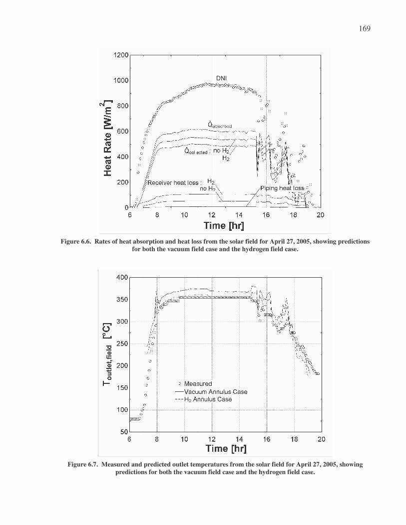
169

Figure 6.6. Rates of heat absorption and heat loss from the solar field for April 27, 2005, showing predictions


Figure 6.7. Measured and predicted outlet temperatures from the solar field for April 27, 2005, showing


170

Figure 6.8. Rates of heat absorption and heat loss from the solar field for March 12, 2005, showing


Figure 6.9. Measured and predicted outlet temperatures from the solar field for March 12, 2005, showing


171

Assuming 50% of the collector field has been compromised by hydrogen permeation in the

annular space at a pressure of 1 [torr] results in a decrease in predicted solar field outlet

temperature of about 8 – 9 [°C], on average, through the majority of the operating day. The

outlet temperature predictions for the hydrogen field case show much closer agreement with

plant data than predictions that assume no hydrogen permeation (base case) for all days except

the day in March, in which the hydrogen field case under-predicts the solar field outlet

temperature.

The differences in outlet temperature predictions shown as a result of hydrogen permeation may

appear at first to be small. As has been shown by Forristall (2003), losses from the solar field

due to heat transfer through the HCE are small when compared to the concentrated radiation

absorbed. In Figure 6.3, for example, the heat flux incident on the receiver tubes (Qabsorbed) on

June 11, 2005 ranges from about 600 – 650 [W/m2] through mid-day. By comparison, receiver

heat losses (due to convection and radiation from the glass envelope to the environment) in the

evacuated annulus case are about 55 [W/m2], an order of magnitude smaller than the heat flux

incident on the tubes. Heat losses for the hydrogen case increase to about 110 [W/m2], roughly a

100% increase in heat loss as compared to the vacuum case. Since the magnitude of heat flux

incident on the receiver tubes is large compared to the magnitude of receiver heat loss, a 100%

increase in thermal losses translates to about a 10% decrease in thermal energy collection by the

solar field. This effect is evidenced by the change in Qcollected shown in Figure 6.3, which peaks

at about 605 [W/m2] for the vacuum field case but peaks at only about 550 [W/m2] for the

hydrogen field case. The following section quantifies the impact of increased losses on the net

electric power generation capability of the plant.

172

6.4 Effect on Electric Power Output

Figures 6.11 through 6.14 show power output predictions from the linked solar field – power

cycle model for four days through the spring and early summer of 2005, showing predictions for

both the vacuum field case and the hydrogen field case.

Figure 6.10. Measured and predicted gross electric power for June 11, 2005, showing predictions for both the

vacuum field case and the hydrogen field case.

173

Figure 6.11. Measured and predicted gross electric power for May 20, 2005, showing predictions for both the


Figure 6.12. Measured and predicted gross electric power for April 27, 2005, showing predictions for both the


174

Figure 6.13. Measured and predicted gross electric power for March 12, 2005, showing predictions for both

the vacuum field case and the hydrogen field case.

The predicted difference in power output due to hydrogen permeation in 50% of the solar field is

about 4 [MW] on the summer days (May and June) and 3.5 [MW] during the mid-morning and

afternoon on April 27, or 10 – 11% of the rated gross output (35 [MW]) of the plant.

It may seem odd that the temperature at the solar field outlet appeared not to be significantly

affected by the hydrogen, but that the power does appear to be significantly affected. The

magnitude of the change in power output can be confirmed with a few rough calculations.

Recall from section 6.3 that the difference in collected radiation between the vacuum case and

the hydrogen case on June 11 was about 55 [W/m2]. Multiplied by the aperture area of the solar

field (roughly 182,000 m2), the difference in Qcollected translates to a change in heat supplied to

175

the power cycle of about 10 [MW]. Assuming the first law efficiency of the Rankine power

cycle is about 37%, the potential change in power output that could accompany this change in

absorbed energy is 3.7 [MW].

While the predicted solar field outlet temperatures and gross power production for the hydrogen

field case agree closely with measured data on days in May and June, the agreement is not as

favorable on the day in March, when the solar field outlet temperature is lower. The absorber

tubes are each equipped with hydrogen getter strips, which help collect hydrogen in the annulus.

It is believed that the getter strips retain more hydrogen at lower temperatures as compared to

higher temperatures, thus reducing the ‘hydrogen effect’ during evening hours and days in the

off-summer seasons (Price, personal communication, 2005).

6.5 Conclusions

The hydrogen field case predictions for solar field outlet temperature and power production

agree well with measured data during summer and spring days. However, while the correlation

provides strong evidence for the argument that hydrogen permeation or other compromise of the

annulus vacuum has affected the performance of the solar field, it does not prove that the lower

outlet temperatures observed in 2005 are caused by hydrogen permeation. Agreement between

model predictions and measured data alone can not be used to conclude that the behavior

observed in the field is driven by the conditions implemented in the simulation. It is possible

that the decline in solar field performance observed in the years between 1998 and 2005 is

caused not by an increase in thermal losses from the field, but by a decrease in the amount of

176

energy absorbed by the receiver tubes. For example, for June 11, 2005, it was observed that

outlet temperature and gross power predictions agree with measured data when the energy

collected by the solar field reaches a high of about 550 [W/m2]. The same rate of energy

collection could be achieved in the simulation by assuming that all of the HCEs in the field are

evacuated and that absorbedQ� , the rate of energy absorption, has decreased by 10%. The rate of

energy absorption would decrease by 10% if any of the following surface properties or

performance factors, or a combination thereof, were to decrease by 10%:

• the cleanliness of the mirrors;

• the reflectivity of the mirrors;

• the cleanliness of the HCE receiver tubes;

• the absorbtivity of the HCE selective surface coating;

• the transmissivity of the HCE glass envelope.

Field measurements of the annulus pressure in the receiver tubes and confirmation of the gas(es)

present in the annulus would greatly improve the ability to quantify the actual effect of hydrogen

permeation in the field. Performance tests of HCE and mirror surface properties are necessary to

confirm that the decline in performance can not be attributed to these factors.

The analysis of thermal losses presented in this chapter does not take into account any variation

in the pressure of the hydrogen in the receiver tubes. Heat losses from the hydrogen receiver

tubes were modeled assuming the pressure in the annulus was greater than or equal to about 1

[torr] at all bulk fluid temperatures. If the actual pressure of hydrogen in the receiver tubes is

much smaller than 1 [torr], heat losses from the tube will be significantly decreased.

177

This analysis also does not take into consideration the fact that hydrogen permeation is more

prevalent in the high temperature end of the solar field. In the solar field model (see Chapter 2),

heat losses are estimated assuming the overall heat loss from the field is a weighted average of

the heat loss contributed by each type of HCE (vacuum annulus, lost vacuum, H2 in annulus) in

the field. Heat losses from each type are estimated over the inlet and outlet temperatures to the

entire solar field.

The high thermal losses that occur as a result of hydrogen permeation could be greatly mitigated

by addition of another gas to the annulus at a much higher pressure (10 to 100 [torr]). An inert

gas such as argon has been proposed for this purpose (Price, personal communication, 2005). A

mixture of hydrogen and argon in the annulus will act like a pure ideal gas with a pseudo

molecular weight equal to the mole fraction weighted average value. In other words, a mixture

of hydrogen and argon that is heavily weighted towards argon will behave very much like pure

argon. The thermal conductivity of argon gas is much lower than that of hydrogen; thus, thermal

losses from the field could be reduced by injection of argon into the annulus. Injecting argon

into the annulus will not stop the permeation of hydrogen through the absorber, since this

diffusion process is driven by the partial pressure difference for hydrogen.

178

7 Optimized Control of Solar Field Flow Rate

7.1 Introduction

At the SEGS VI plant, the flow rate of

the circulating heat transfer fluid is

manually controlled by a plant operator

(Figure 7.1). The plant operators

typically increase the flow rate

gradually through the solar field during

start up, maintain a relatively constant

flow through mid-day operation, and

gradually lower the flow rate late in the

day in preparation for power plant shut

down. High flow rates improve the heat transfer coefficient in the HTF – steam heat exchangers,

but result in higher pumping parasitics and lower solar field outlet temperatures. Conversely,

low flow rates will result in smaller pumping parasitics and higher solar field outlet

temperatures, but reduce the heat transfer coefficient in the HTF – steam heat exchangers. At

very low flow rates, operators may further run the risk of degrading the heat transfer fluid, or

creating thermal shock or HTF expansion in the solar field equipment great enough to break the

receiver tubes. Plant operators rely on observation of temperatures in the solar trough field,

observation of weather conditions (such as cloud cover), and their individual experience and best

judgment to balance the competing temperature and flow rate requirements.

Figure 7.1. Solar field plant operator (Source: KJC

Operating Company, 2004)

179

The objective of this section is to explore impact of the solar field flow rate on electric power

produced by the cycle. The net electric power output from the system, at a given incident

radiation, is a function of the system efficiency, defined as the product of the solar field

efficiency and the power cycle efficiency. The efficiency of the solar field decreases with

increasing outlet temperature. The efficiency of the power cycle increases with increasing outlet

temperature. The magnitude of these competing trends is such that the net change in system

efficiency with outlet temperature is small. Therefore, operation over a wide range of solar field

temperatures and flow rates will produce little discernible difference in the electricity output.

This behavior is observed in simulations of the solar field and power cycle combined system,

employing various strategies for control of the solar field.

7.2 Solar Field, Power Cycle Efficiency with Flow Rate

The instantaneous efficiency of the solar field is defined as the rate of useful energy gain of the

solar field over the incident radiation on the absorber tubes:

colfield

aper incident

Q

A I=

�

η (7.1)

where

ηfield = the instantaneous solar field efficiency

aperA = total aperture area (product of mirror width and mirror length) of solar field [m2]

Iincident = corrected incident solar radiation [W/m2]

colQ� = rate of useful thermal energy gain [W]

180

The rate of useful energy gain of the solar field, colQ� , is the product of the HTF mass flow rate

and the enthalpy change across the field expressed on a per unit solar field aperture area basis:

, ,( )col HTF SF out SF inQ m h h= ⋅ −� � (7.2)

where

HTFm� = mass flow rate of heat transfer fluid through the field [kg/s]

,SF inh = inlet enthalpy of heat transfer fluid [J/kg]

,SF outh = outlet enthalpy of heat transfer fluid [J/kg]

The incident radiation is the product of the direct normal insolation and the modified angle of

incidence on the trough plane:

cos( )incidentI DNI IAMθ= ⋅ ⋅ (7.3)

where


cos( )θ = cosine of the angle of incidence between beam radiation and aperture normal

IAM = incidence angle modifier (see Chapter 2)

Figure 7.2 shows solar field efficiency versus solar field outlet temperature, at various lines of

constant incident radiation and field flow rate for both intact collector tubes and degraded

collector tubes. The intact collector tube case assumes all collectors have retained their as-built

vacuum condition within the annulus. The degraded collector tube case assumes that 50% of the

collector field has H2 infiltration in annulus at a pressure of 1 [torr], as described in Chapter 6.

181

Figure 7.2. Solar field efficiency versus solar field outlet temperature, at various lines of constant incident

radiation [W/m2]. All lines truncate at a mass flow rate of 500 [kg/s] on the low temperature end and 240

[kg/s] on the high temperature end.

At a specified radiation level, higher efficiency of the solar field results from lower solar field

outlet temperatures. This trend is dictated by thermal losses from the HCE, which increase with

increasing fluid temperature (see Figures 2.18 – 2.20). The magnitude of change in the solar field

efficiency is greater for the collectors that have been compromised by hydrogen in the annulus

than for those for which the annulus is evacuated. For the vacuum case, the decrease in solar

field efficiency with increasing solar field outlet temperature is relatively small. At a constant

incident radiation of 950 [W/m2] over a range of flow rates commonly observed in the field

(from 500 [kg/s] to 240 [kg/s]), without hydrogen permeation, the efficiency of the solar field

will decrease 1.4% from 62.4% to 61.0%. Over the same range, with hydrogen permeation, solar

field efficiency decreases 1.7 % from 56.4% to 54.7%. It should be noted that Figure 7.2 shows

182

solar field outlet temperatures above the maximum permissible operating temperature of the

plant (400 [°C]).

The gross efficiency of the power cycle is defined as the ratio of the electrical power (gross)

produced by the cycle to the thermal energy provided to the cycle, which is equal to the rate of

useful energy collection by the solar field:

,( )

electricpower gross

HTF SFout SFin

W

m h hη =

⋅ −

�

� (7.4)

The net efficiency of the power cycle is defined as the ratio of the net electrical power produced

by the cycle to the thermal energy provided to the cycle, where the net power equals the gross

power minus electrical power supplied to the heat transfer fluid pumps ( HTFpumpsW� , Equation

2.28), condenser water pumps ( CTpumpsW� , Equation 4.12), cooling tower fans ( CTfansW� , Equation

4.24), and working fluid pumps ( CPW� and DPW� , Equation 3.84 – 3.85):

parasitic HTFpumps CP DP CTpump CTfansW W W W W W= + + + +� � � � � � (7.5)

,( )

electric parasitic

power net

HTF SFout SFin

W W

m h hη

−=

⋅ −

� �

� (7.6)

Figure 7.3 shows gross power cycle efficiency versus solar field outlet temperature, for the same

lines of constant incident radiation as shown in Figure 7.2. Thermal losses from the HTF –

steam heat exchanger jackets to the ambient air (see Chapter 5.6) represent a significant loss of

available thermal energy to the plant; shown in Figure 7.2 are the gross efficiency of the power

183

cycle assuming no jacket thermal losses, as well as the gross efficiency assuming jacket losses as

calculated from Equations 5.17 – 5.18.

Figure 7.3. Power cycle efficiency (gross) versus solar field outlet temperature, at various lines of constant

incident radiation. All lines represent mass flow rate between 500 [kg/s] at the low temperature end and 240

[kg/s] at the high temperature end.

The gross efficiency of the power cycle increases with the increasing solar field outlet

temperature. The degree to which power cycle gross efficiency is affected by solar field outlet

temperature depends on whether or not thermal losses from the HTF – steam heat exchanger

jackets are included in the analysis. When jacket losses are included, the increase in efficiency

of the power cycle is offset by the subsequent increase in heat transfer to the surrounding

environment, as thermal losses from the jacket increase with increasing HTF temperature. For

incident radiation of 950 [W/m2] over the range of flow rates commonly observed in the field

184

(from 500 [kg/s] to 240 [kg/s]), without jacket losses, the gross efficiency of the SEGS VI power

cycle increases 0.5%, from 38.5% to 39.0%. When jacket losses are included, the gross

efficiency of the SEGS VI power cycle increases from 34.4% to 34.8%.

The change in net cycle efficiency versus solar field outlet temperature, for a constant incident

radiation, is shown in Figure 7.4.

Figure 7.4. Power cycle efficiency (net) versus solar field outlet temperature, at various lines of constant

incident radiation. All lines represent mass flow rate between 500 [kg/s] at the low temperature end and 240

[kg/s] at the high temperature end.

Parasitic power requirements decrease substantially with reductions in solar field mass flow rate

and consequent reductions in the working fluid (steam) mass flow rate. As a result, the net

efficiency of the plant shows a dramatic increase with increasing solar field outlet temperature.

At a constant incident radiation of 950 [W/m2], over a range of solar field mass flow rates from

500 [kg/s] to 240 [kg/s], without jacket losses, the estimated net efficiency of the power cycle

185

will increase 3.3%, from 33.4% to 36.7%. With jacket losses, the net efficiency of the power

cycle will increase from 2.6%, from 30.1% to 32.7%.

The system efficiency is defined as the ratio of the electrical power produced by the cycle to the

thermal energy supplied to the cycle, or the product of the solar field efficiency and the power

cycle efficiency:

( )

electric electricsystem

incident aper HTF SFout SFin

W W

I A m h hη = =

⋅ −

� �

�

( )HTF SFout SFinm h h−⋅�

aper

incident

A

I (7.7)

, ,system gross field power grossη η η= ⋅ (7.8)

, ,system net field power netη η η= ⋅ (7.9)

Figure 7.5 shows gross system efficiency versus solar field outlet temperature, for the same

levels of constant incident radiation as shown in Figures 7.2 and 7.3.

186

Figure 7.5. Gross efficiency of the solar field-power cycle system versus solar field outlet temperature, at

various lines of constant incident radiation.

The efficiency trends in the solar field and the power cycle with solar field outlet temperature

work against each other within the range of flowrates between 240 [kg/s] and 500 [kg/s]. In all

cases, the gross system efficiency shows a slight decrease with increasing solar field outlet

temperature. As the overall efficiency of the system improves, the effect of solar field outlet

temperature on system efficiency diminishes slightly. In all scenarios, the change in gross

system efficiency over the given range of HTF flow rates is very small, on the order of 0.2% or

less. For example, the change in gross efficiency of the system over the normal range of

operating flow rates, for a constant incident radiation of 950 [W/m2] with no jacket heat losses

and no hydrogen permeation, is only 0.2%, from 24.0% at 500 [kg/s] to 23.8% at 240 [kg/s].

Figure 7.6 shows net system efficiency with solar field outlet temperature.

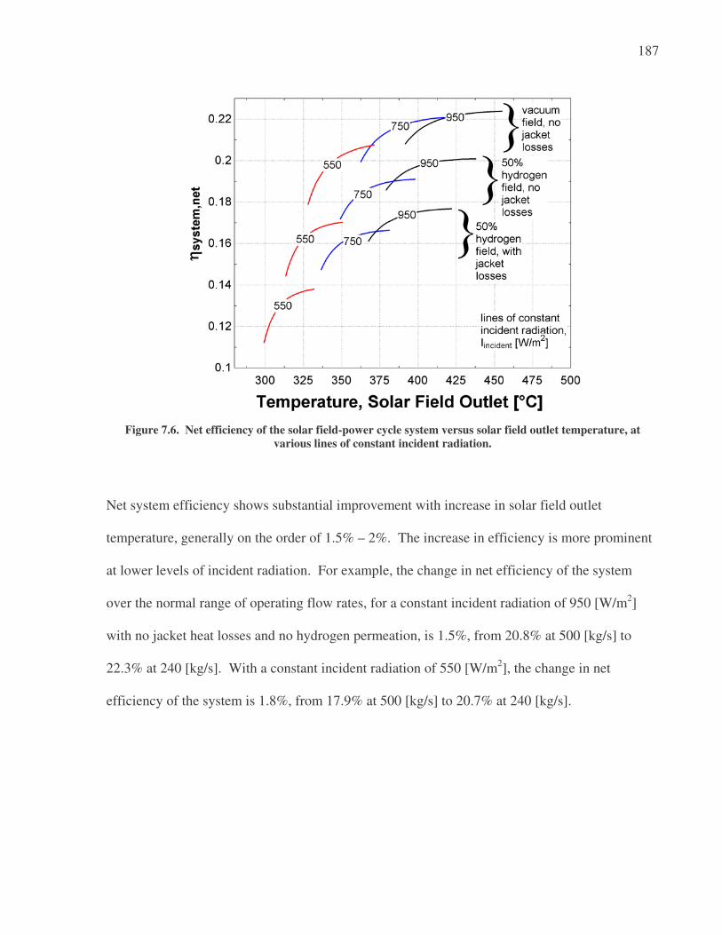
187

Figure 7.6. Net efficiency of the solar field-power cycle system versus solar field outlet temperature, at

various lines of constant incident radiation.

Net system efficiency shows substantial improvement with increase in solar field outlet

temperature, generally on the order of 1.5% – 2%. The increase in efficiency is more prominent

at lower levels of incident radiation. For example, the change in net efficiency of the system

over the normal range of operating flow rates, for a constant incident radiation of 950 [W/m2]

with no jacket heat losses and no hydrogen permeation, is 1.5%, from 20.8% at 500 [kg/s] to

22.3% at 240 [kg/s]. With a constant incident radiation of 550 [W/m2], the change in net

efficiency of the system is 1.8%, from 17.9% at 500 [kg/s] to 20.7% at 240 [kg/s].

188

7.3 Impact of Flow Rate Control on Power Output

The comprehensive solar field-power cycle simulation model has been run for two days in 2005

using the following four flow rate scenarios:

1) The flow rate recorded in the plant data for the day is used;

2) The flow rate is set constant at 300 [kg/s] ;

3) The flow rate is controlled for a constant solar field outlet temperature of 390 [C];

4) The flow rate is controlled for a constant temperature difference over the solar field of 100 [C].

The solar field flow rates and resultant solar field outlet temperature for each control scheme are

compared for May 20, 2005, in Figures 7.7 and 7.8, and for June 11, 2005, in Figures 7.9 and

7.10. The gross power outputs resulting from the four selected control strategies are shown in

Figures 7.11 for May 20, 2005, and in Figure 7.12 for June 11, 2005.

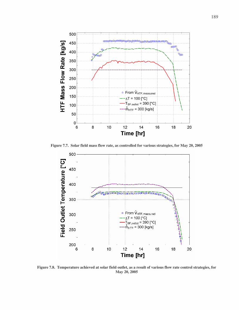
189

Figure 7.7. Solar field mass flow rate, as controlled for various strategies, for May 20, 2005

Figure 7.8. Temperature achieved at solar field outlet, as a result of various flow rate control strategies, for

May 20, 2005

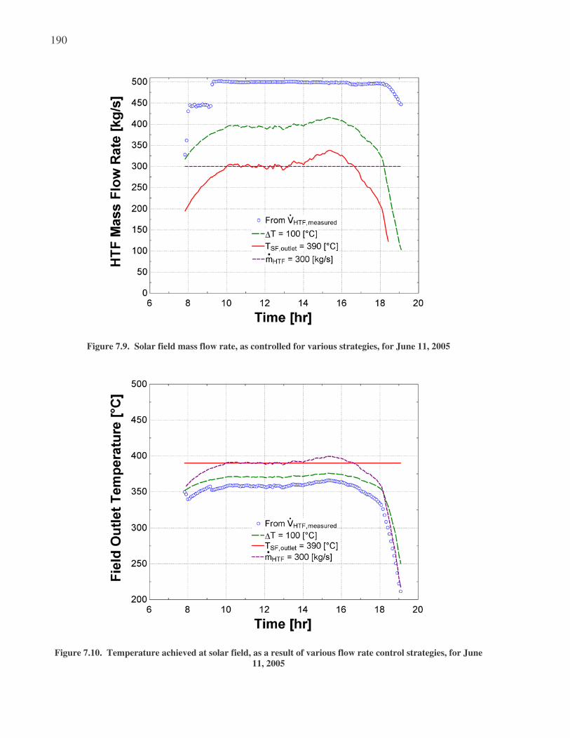
190

Figure 7.9. Solar field mass flow rate, as controlled for various strategies, for June 11, 2005

Figure 7.10. Temperature achieved at solar field, as a result of various flow rate control strategies, for June

11, 2005

191

Figure 7.11. Gross and net electric power production predicted as a result of different flow rate control

strategies, for May 20, 2005. Measured gross electric power produced by the plant is shown for reference.

Figure 7.12. Gross and net electric power production predicted as a result of different flow rate control

strategies, for June 11, 2005. Measured gross electric power produced by the plant is shown for reference.

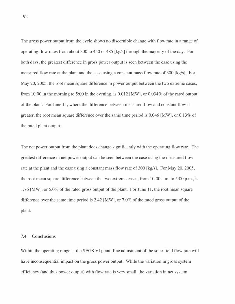
192

The gross power output from the cycle shows no discernible change with flow rate in a range of

operating flow rates from about 300 to 450 or 485 [kg/s] through the majority of the day. For

both days, the greatest difference in gross power output is seen between the case using the

measured flow rate at the plant and the case using a constant mass flow rate of 300 [kg/s]. For

May 20, 2005, the root mean square difference in power output between the two extreme cases,

from 10:00 in the morning to 5:00 in the evening, is 0.012 [MW], or 0.034% of the rated output

of the plant. For June 11, where the difference between measured flow and constant flow is

greater, the root mean square difference over the same time period is 0.046 [MW], or 0.13% of

the rated plant output.

The net power output from the plant does change significantly with the operating flow rate. The

greatest difference in net power output can be seen between the case using the measured flow

rate at the plant and the case using a constant mass flow rate of 300 [kg/s]. For May 20, 2005,

the root mean square difference between the two extreme cases, from 10:00 a.m. to 5:00 p.m., is

1.76 [MW], or 5.0% of the rated gross output of the plant. For June 11, the root mean square

difference over the same time period is 2.42 [MW], or 7.0% of the rated gross output of the

plant.

7.4 Conclusions

Within the operating range at the SEGS VI plant, fine adjustment of the solar field flow rate will

have inconsequential impact on the gross power output. While the variation in gross system

efficiency (and thus power output) with flow rate is very small, the variation in net system

193

efficiency is much more pronounced. Net system efficiency increases with decreasing solar field

mass flow rate and increasing solar field outlet temperature; the primary driving force behind this

trend is the decrease in parasitic power required for HTF pumps and working fluid pumps at

smaller flow rates. Further study of the parasitic power requirements and efficiency of the HTF

pumps and working fluid pumps is warranted to more accurately quantify the net power increase

resulting from a change in solar field operating strategy.

This study has not addressed the consequences of solar field outlet temperature on the integrity

of the heat transfer fluid and collector field equipment. The potential exists for increased

likelihood of collector failure or heat transfer fluid degradation as a result of operating at a higher

solar field outlet temperature. These considerations must be understood as well before a

particular solar field flow rate control strategy can be recommended.

194

8 Alternative Condensers

8.1 Introduction

Heat rejection from the exhaust stream in the SEGS VI power cycle is currently accomplished by

heat exchange in a shell-and-tube surface condenser with circulating cooling water. The cooling

water is cooled by evaporation in an induced draft cooling tower. Makeup water must be

supplied to the cooling water stream to compensate for water loss due to evaporation. Water

consumption for makeup feedwater, cooling water, and other site services was estimated in the

design of the plant at 450 acre-feet per year (Kearney et al, 1988); water consumption adversely

impacts the operating costs of the plant since the SEGS plants are located in the desert, where the

natural water supply is scarce.

There are alternative means for condensing steam that do not require makeup water. An A-frame

air cooled condenser (ACC), for example, condenses steam through several finned tubes with

forced air convection on the outer surfaces of the tubes. The primary advantage of air cooled

condensing is the elimination of water consumption for cooling water makeup. Another

advantage is elimination of the cooling tower plume. Elimination of the cooling tower plume

presents a unique benefit at the SEGS plants, as condensation from the cooling tower plume can

reduce the optical efficiency of the SCA mirrors closest to the cooling tower. The primary

disadvantage of air cooled condensing is that heat transfer by forced air convection is a less

effective heat transfer process than evaporative heat transfer. Therefore, larger heat exchanger

areas and greater fan power will be required to achieve heat rejection from the cycle comparable

to the design state. The performance of the air cooled condenser is also more dramatically

195

influenced by dry bulb temperature than the wet cooling tower, which is a wet bulb driven

process.

This chapter will address the design and performance of an air cooled condenser unit suitable for

replacement of the surface condenser and cooling tower in place at the SEGS plants. Previous

work in air cooled condenser modeling and performance evaluation (Conradie and Kroger, 1995)

provides the base case performance characteristics of a single ACC unit. The number of air-

cooled condensing units required for the SEGS VI plant is calculated assuming each condensing

unit in the array has the same performance. An optimum size for the ACC array is selected to

maximize the net power output from the air cooled cycle. Variation of the air-cooled cycle

performance and circulating cooling water cycle performance is determined for one year, using

monthly design ambient temperature and mean coincident wet bulb temperatures for each month.

The performance of the air-cooled condenser is simulated with the solar field and power cycle

for June 20 of 1998. The economic merit of the air cooled system is considered by evaluating

and comparing the cost of condenser makeup water for the given day in June and the opportunity

cost of lost power production due to higher condensing pressures.

8.2 Air Cooled Condenser Design

Discussion of the design of an A-frame air cooled condenser is based on condenser modeling for

similar applications from Conradie and Kroger (1995). In this work, a physical model for a

forced draft air cooled condenser is derived, which is based on mass and energy conservation

equations. The physical parameters and operating conditions for a single unit analyzed in this

design study are listed in Table 8.1.

196

Table 8.1. Example ACC Parameters and Operating Conditions

(Source: Conradie and Kroger, 1995)

Fin Tube

Outer diameter 69.9 mm Outer diameter 38.1 mm

Inner diameter 40.3 mm Inner diameter 35.1 mm

Thickness 0.35 mm Length 10 m

Pitch * 3.63 (row 1) 2.54 (row 2)

mm Number * 152 (row 1) 153 (row 2)

-

Material Aluminum Material Steel

Thermal conductivity 204 W/m-K Thermal conductivity 50 W/m-K

Apex angle 30 °

Width of tube row 11.659 m

Design point operating conditions

Ambient temperature 15.6 °C

Atmospheric pressure 86.4 kPa

Volumetric air flow rate 529.4 m3/s

Air mass flow rate 540.8 kg/s

Fan power 101 kW

Steam mass flow rate 4.675 kg/s

Saturated steam temperature 60 °C

Heat dissipated 11.036 MW

Air exit temperature 37.3 °C

* The pitch and number of tubes are adjusted to induce the same condensing pressure in each row of tubes.

It is assumed that the basic design of the air-cooled condenser in the Conradie and Kroger study

is similar to the design that could be applied at the SEGS plants. The physical parameters and

performance calculated in this study are taken as the base case and applied for the operating

conditions at the SEGS plants.

The effectiveness of the condenser is expressed as the heat transfer through the condenser over

the maximum heat transfer possible:

,( )air air SAT steam amb

Q

m cp T Tε =

⋅ −

�

� (8.1)

197

The heat transfer per unit, the mass flow rate of air per unit, and the operating ambient air

temperature and condensing steam temperature are specified in Table 8.1. Using a specific heat

of air of 1.007 [kJ/kg-K], the effectiveness of the condenser is found to be 0.425. The UA of the

condenser is found using the effectiveness-NTU relation for heat exchangers with phase change:

1 exp( )NTUε = − − (8.2)

air air

UANTU

m cp=

⋅� (8.3)

From Equations (8.2) and (8.3), the number of transfer units for the condenser is found to be

0.554, and the corresponding UA is 324 [kW/K].

The condenser is sized for application at SEGS by adding identical modules of the design

condenser unit to an array. The performance and parasitic requirements of each condenser in the

array are identical. The same air mass flow rate specified in the design study example is used for

each condensing unit in the SEGS simulation. Assuming fluid properties do not change

significantly with temperature and that the heat transfer coefficient on the water side is much

larger than the heat transfer coefficient on the air side, it is assumed that the UA of the condenser

array applied under the operating conditions at SEGS would not vary significantly from the

design example value. The number of transfer units and the effectiveness of the condenser will

have the same values as those calculated in the design study example as well.

The effectiveness of the air cooled condenser establishes the relationship between the steam-to-

air heat transfer and the maximum heat transfer possible for the given air and steam inlet

temperatures:

198

( ), , ,

,( )

steam unit steam in steam out

air air SAT steam ambient

m h h

m cp T Tε

−=

−

�

� (8.4)

It is assumed that the total mass flow of steam is distributed evenly among the condensers in the

array, and that the steam leaves the condenser as saturated liquid:

,steam unit steam unitsm m N=� � (8.5)

, ,( , 0)steam out SAT steamh h T x= = (8.6)

Simultaneous solution of Equations 8.4 – 8.6 determines the condensing temperature (and

corresponding condensing pressure) of the steam. A design ambient air temperature of 42.9 [°C]

is chosen from the ASHRAE Fundamentals design conditions for Edwards Air Force Base

(ASHRAE Fundamentals, 2005).

Parasitic fan power required for the condensing array is calculated assuming each unit in the

array uses the same fan, with the same air mass flow rate and power requirements as the fan cited

in the Conradie and Kroger study:

, (101 [kW])fan ACC unitsW N= ⋅� (8.7)

Figure 8.1 shows the condensing pressure and temperature achieved versus the number of air

cooled condenser units in use in an array. For the results shown in Figure 8.1, the power cycle is

199

supplied with a constant HTF mass flow rate of 400 [kg/s] and a constant HTF temperature of

390 [°C].

Figure 8.1. Condensing pressure and corresponding condensing temperature versus number of air cooled

condenser (ACC) units in an array.

As the number of condensing units increases, the condensing pressure approaches an asymptotic

limit. The limiting condensing pressure in an air cooled condenser will be the saturation pressure

corresponding to the ambient air temperature. The ambient air temperature chosen for the design

case is higher than the condensing temperature specified for SEGS VI at rated power (41.5 [°C]).

Since the design ambient air temperature exceeds the designed condensing pressure for the

power cycle, there is no combination of ACC units that would return a lower condensing

pressure than the current cooling configuration.

200

8.3 Optimum Size of Air Cooled Condenser for SEGS VI

Even if it were possible to condense steam in the air cooled condenser at the ambient air

temperature, the increase in parasitic fan power required to reach this temperature would

outweigh the increase in gross power from the cycle. There must be an optimum condensing

pressure at which the net power output from the cycle is at a maximum. Figure 8.2 shows gross

and net power output from the air cooled condensing cycle as a function of the condensing

pressure. For reference, the net power output from the current cycle configuration operating at

the given condensing pressure is computed as well. For this analysis, the flow rate of the

circulating cooling water is reduced to meet the condensing pressure given; all other parameters

are held constant.

Figure 8.2. Gross cycle power, net cycle power with cooling tower, and net cycle power with air cooled

condenser, versus condensing pressure and condensing temperature.

201

The maximum net plant power that could be achieved, using the ACC unit design as detailed in

Chapter 8.2, is 29.8 [MW], at a condensing temperature of 0.17 [bar]. An array of 18 ACC units

is required to achieve this condensing pressure. This design represents a decrease in net power

of 1.3 [MW] compared to a system with the existing cooling tower operating under a reduced

cooling water flow to achieve the same condensing pressure. This design also represents a

decrease in net power of 2.6 [MW] from the existing cooling tower operating at maximum

cooling water flow, under same ambient air and HTF temperature and mass flow conditions.

8.4 Annual Performance of Condensers

Heat rejection systems are heavily influenced by ambient air conditions. Since evaporative

transfer is driven by the dryness of the air, the cooling tower performance will improve with the

difference between wet bulb and dry bulb temperature. Conversely, the air cooled condenser

performance is a function not of the wet bulb temperature, but of the dry bulb temperature alone.

Lower ambient temperatures produce better performance in an air cooled condenser, as the

ambient temperature represents the maximum condensing temperature that could theoretically be

reached.

Table 8.2 lists monthly design dry bulb and mean coincident wet bulb temperatures for Edwards

Air Force Base, located about ten miles from the Kramer Junction SEGS site.

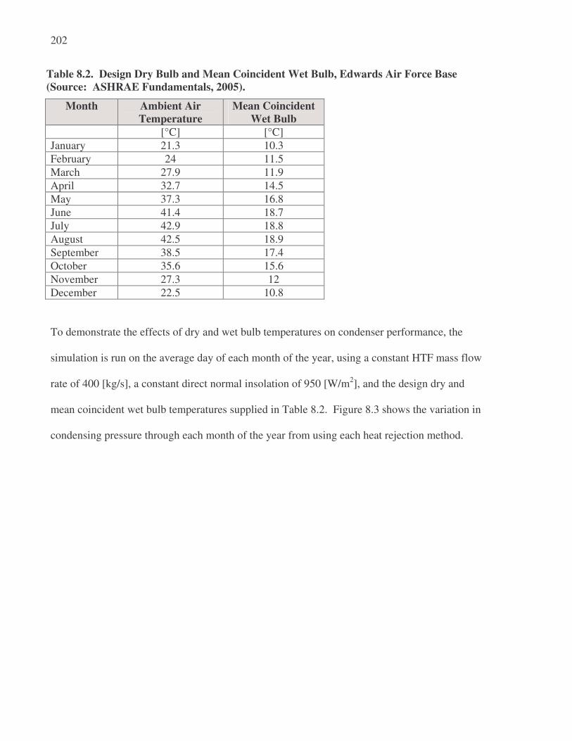
202

Table 8.2. Design Dry Bulb and Mean Coincident Wet Bulb, Edwards Air Force Base

(Source: ASHRAE Fundamentals, 2005).

Month Ambient Air

Temperature

Mean Coincident

Wet Bulb

[°C] [°C]

January 21.3 10.3

February 24 11.5

March 27.9 11.9

April 32.7 14.5

May 37.3 16.8

June 41.4 18.7

July 42.9 18.8

August 42.5 18.9

September 38.5 17.4

October 35.6 15.6

November 27.3 12

December 22.5 10.8

To demonstrate the effects of dry and wet bulb temperatures on condenser performance, the

simulation is run on the average day of each month of the year, using a constant HTF mass flow

rate of 400 [kg/s], a constant direct normal insolation of 950 [W/m2], and the design dry and

mean coincident wet bulb temperatures supplied in Table 8.2. Figure 8.3 shows the variation in

condensing pressure through each month of the year from using each heat rejection method.

203

Figure 8.3. Condensing pressure obtained in cooling tower and air cooled condenser through one year, using

ambient air temperature and mean coincident wet bulb temperature from ASHRAE Fundamentals for

Edwards Air Force Base.

The effect of ambient temperature on condensing pressure is clearly seen in Figure 8.3. Through

the course of the year, the condensing pressure from air cooled condensing can range from 0.035

– 0.176 [bar]. Conversely, changes in the condensing pressure from circulating cooling water

condensing are much less dramatic; condensing pressure ranges from 0.026 – 0.077 [bar]

throughout the year in this cycle configuration.

Figure 8.4 shows gross power and net power production from the system using each heat

rejection method, as a function of design ambient air temperature and mean coincident wet bulb

temperature.

204

Figure 8.4. Gross power and net power resulting from the cycle for the mean day of each month of the year,

using dry bulb and mean coincident wet bulb temperatures from ASHRAE Fundamentals for Edwards Air

Force Base.

Performance of the power cycle with air cooled condensing suffers most in the summer; the

difference in net power between the two cooling configurations in June is 2.7 [MW]. During

January, the net performance difference between the two heat rejection methods is 1.1 [MW].

Unfortunately, this performance trend is ill-suited for the SEGS plants, which are designed to be

most productive during the summer months.

It should be noted that, for the monthly simulation results shown in Figures 8.3 and 8.4, the

condensing pressure for the cooling tower case is calculated assuming the circulating cooling

water is flowing at design capacity and that both cooling tower fans are operating at high speed.

The condensing pressure in the air cooled condenser is also computed assuming all fan units are

operating at full speed for the full year. These conditions do not necessarily represent optimal

205

operating conditions at all times of the year and are used here only for the sake of a base

performance comparison from one month to the next.

8.5 Simulation Using Air Cooled Condenser

Figure 8.5 shows simulation results for gross and net power production simulation from the solar

field – power cycle system for June 20, 1998, for both the water cooled cycle and the air cooled

cycle.

Figure 8.5. Gross and net power production predicted from measured plant data from June 20, 1998, for

both the water cooled cycle (cooling tower) and the air cooled cycle (ACC).

The root mean square difference in gross power production between the two cycles (computed

between 10 a.m. and 4 p.m.) is about 0.54 [MW]; root mean square difference in net power

production between the two cycles is about 1.44 [MW]. The cumulative loss in net power

206

production over the entire day as a result of air cooling, from the model predictions, is about 14.8

[MWh].

Cooling water makeup requirements are calculated from the change in mass fraction of moisture

in the air between cooling tower intake and cooling tower exhaust. The mass fraction of water in

the cooling tower intake is evaluated from the partial pressure of the moisture in the air, which is

determined from the relative humidity and saturation pressure at the ambient air temperature:

( , )v SAT ambient

P R P water T= ⋅ (8.8)

where

Pv = partial pressure of water vapor in intake air [-]

R = relative humidity of intake air [-]

0.622 vintake

atm v

P

P Pω =

− (8.9)

where

Patm = atmospheric pressure (1 [atm])

The mass fraction of water in the cooling tower exhaust air is evaluated assuming the water is

saturated at the outlet temperature of the air:

,

,

( , )0.622

( , )

SAT air out

exhaust

atm SAT air out

P water T

P P water Tω =

− (8.10)

207

The rate of water loss is the product of the mass flow rate of the air and the difference in water

mass fraction between intake and exhaust:

( )makeup air exhaust intakem m ω ω= −� � (8.11)

For the water cooled cycle, cooling water makeup requirements are estimated at 244,000

gallons/day for June 20, 1998.

8.6 Economics of Dry Condensing

The Kramer Junction SEGS facility contracts with the Antelope Valley-East Kern Water Agency

(AVEK) to supply California aqueduct water to the facility (Kearney et al, 1988). The 2005 cost

of untreated water to the cooling tower is $500/acre-foot (1.53E-03 [$/gal]); cost of treatment

chemicals for cooling tower water is approximately 1.65E-04 [$/gal] (Gummo, 2006). The total

cost of cooling tower makeup water, from the combined purchase costs of raw water and

treatment chemicals, is estimated at 1.7E-03 [$/gal]. For June 20, 1998, the savings in cooling

water makeup resulting from use of air cooled condensing would amount to $414 / day.

Assume the opportunity cost of the lost power production due to air cooled condensing can be

quantified by the levelized cost of electricity. The levelized cost of electricity from the SEGS

plants was estimated at $0.14/kWh in 2002 dollars (Price, 2003). The levelized cost of

electricity, multiplied by the cumulative loss in net power production over the day, shows

production losses of about $2,090 / day resulting from air cooled condensing. By this analysis,

the cost of the electricity production losses far outweigh the cost savings from reduced water

consumption. Note that this represents a cost/benefits analysis for only one day of the year; the

208

same analysis would have to be performed over several days of the year to estimate the yearly

operating cost savings and cost penalties associated with dry condensing.

8.7 Conclusions

Use of an air-cooled condenser in place of the current cooling configuration would increase the

condensing temperature and pressure of the steam. With a design ambient temperature of 42.9

[°C] and parasitic power requirement of 101 [kW] per unit, an array of 18 A-frame condenser

units would produce optimal net power at a condensing pressure of 0.17 [bar]. Higher parasitic

power requirements, as well as higher condensing pressures, result in a decrease in power from

the air cooled cycle as compared to the water cooled cycle. The performance difference is more

noticeable in the summer months than in the winter months. Air cooled condensing could save

the SEGS VI facility 244,000 gallons of water on a typical summer day, at an estimated cost

savings of about $414. However, the associated decline in net power production is about 14.8

[MWh] / day, which, for a levelized cost of electricity of $0.141/kWh, results in a penalty cost of

about $2,090 / day for a typical summer day.

This study did not include optimization of the design and configuration of the air cooled

condensing unit. The performance characteristics of an existing A-frame air cooled condensing

unit were used as a reference; the effectiveness of the reference unit was found to be 0.425 .

Increasing the effectiveness of the condenser would reduce the parasitic power required to

achieve the same condensing pressure.

209

Capital costs of air cooled condensers were also not included in this study and must be

considered to further weigh the economic merit of dry condensing.

210

9 Conclusions and Recommendations

9.1 Conclusions

A comprehensive model of the SEGS VI solar collector field, power cycle, and heat rejection

system has been written and validated against plant data from both the 1998 and 2005 years of

operation. On clear days in the spring, summer, and fall, the model is capable of predicting the

gross power to within the uncertainty of the plant measurements; predictions are generally off by

no more than 4% of the rated gross power of the plant on the winter days. The model has served

as a tool for understanding the plant’s operating characteristics and has been used to assess

factors that can effectively improve the overall performance of the system. The model has also

provided a basis for quantifying the impacts of potential mechanisms that contribute to

performance degradation, such as partial loss of vacuum in the collector field.

Comparisons of daily gross power production between 1998 and 2005 show substantially

reduced solar field outlet temperatures (by about 8 – 9 [°C]) and gross power production (as

much as 4 [MW]) in 2005 as compared to 1998. This observation is re-enforced by model

simulations, which show excellent agreement with measured solar field outlet temperatures and

power data in 1998 but consistently and significantly over-predict the outlet temperatures and

power production in 2005. The root cause of the decline in the performance of the solar field

during the years between 1998 and 2005 is not known but it is likely the result of a loss in

211

vacuum in the annular space between the receiver tube and the glass enclosure for many of the

receivers in the field. In simulations that assumed 50% of the receiver tubes in the field have

hydrogen in the HCE annular space at a pressure of 1 [torr], good agreement with the measured

data collected in 2005 was obtained.

Overall, the gross system efficiency (without considering parasitic power requirements) was

found to be insensitive to variations in the mass flow rate and solar field outlet temperatures

within the observed operating range of the plant. Therefore, within the operating range at the

SEGS VI plant, fine adjustment of the solar field flow rate will have minimal impact on

optimizing the gross power output. Operation at lower solar field flow rates and higher solar

field outlet temperatures will increase the system net efficiency, as lower solar field flow rates

will require reduced heat transfer fluid parasitic pumping power. However, the flow rate must

still be maintained high enough to keep the solar field outlet temperature below the

recommended maximum operating temperature of the Therminol VP-1 fluid. Other performance

issues influenced by the system operating temperature, such as collector failure and HTF

breakdown, have not been investigated in this study but must be taken into consideration as well

in controlling the flow rate of HTF through the solar field.

Finally, in the interest of reducing water consumption at the plants, the performance impacts of

rejecting heat using air-cooled condensers in place of the current surface condenser and cooling

tower configuration were explored. Based on a design ambient temperature of 42.9 [°C] and

parasitic power requirement of 101 [kW] per unit, an array of 18 A-frame condenser units would

produce optimal net power at a condensing pressure of 0.17 [bar] (condensing temperature of 56

212

[°C]). Higher parasitic power requirements, as well as higher condensing pressures, result in a

decrease in power of about 1.3 [MW] from the air-cooled cycle as compared to the water-cooled

cycle at a condensing pressure of 0.17 [bar]. The performance difference is more noticeable in

the summer months than in the winter months.

9.2 Recommendations for future work

The decline in the performance of the solar field in the years between 1998 and 2005 is well

predicted with the assumption that 50% of the receiver tubes in the field have hydrogen in the

HCE annular space at a pressure of 1 [torr]. However, the agreement between plant data and

model predictions alone can not prove that hydrogen permeation exists at the levels assumed for

the study, nor that hydrogen permeation is the sole cause of the lower solar field outlet

temperatures observed in 1998. Quantification of the annulus pressure of receiver tubes in the

field, confirmation of the gas(es) present in the HCE annular space, and measurement of any

deterioration in the surface properties of the HCE absorber tube, glass envelope, and collector

mirrors would allow for a more conclusive investigation of the noted decline in the performance

of the solar field.

Gross power output from the power cycle has been modeled in detail and validated with plant

data measurements in this study. However, the parasitic power elements (the major elements of

which are the HTF pumps, condenser water pumps, working fluid pumps, and cooling tower

fans) have not been as rigorously modeled. Parasitic power consumption estimates are based on

the power requirements stated for the solar-only rated power output of the plant, known pressure

drops at the plant design state (where available - for working fluid pumps only), and assumed

213

pump reference efficiencies and efficiency curves. Further studies of manufacturer pump

efficiency curves, measured pressure losses, and measured power requirements of individual

pumps/fans are necessary to obtain more accurate parasitic power predictions.

The effects of solar field flow rate control on gross power production are modeled and quantified

in this work. There are further opportunities for optimization of power cycle controls that have

not been explored. The effect of the fraction of the heat transfer fluid directed to the reheater

trains on power production has not been investigated. There is a trade-off between the increased

gross power production resulting from lower condenser pressure and the higher parasitic pump

and fan power required to achieve lower condensing pressures. The optimum net power

production as a function of condensing pressure and parasitic heat rejection power required has

not been investigated.

The design and performance of the air cooled condenser units was taken from a performance

study by Conradie and Kroger (1995). The air cooled condenser unit design was not optimized

for application at SEGS VI in this study. Economic analysis of the trade off between capital cost

and performance of air cooled condensers was not undertaken in this study either.

214

APPENDICES

APPENDIX A

Calculation of Design Parameters: Turbine Efficiency, HTF – Steam and Feedwater Heater UAs APPENDIX B

Dimensions and Performance Parameters for Simulation of SEGS VI Solar Field APPENDIX C

TRNSYS Listing: Type 805 (Solar Field Model) APPENDIX D

TRNSYS Listing: Type 811 (Power Cycle Model) APPENDIX E

TRNSYS Listing: Type 816 (Condenser Model)

APPENDIX F

Contents of Enclosed CD: Modeling Files, Plant Data, and Other Resources

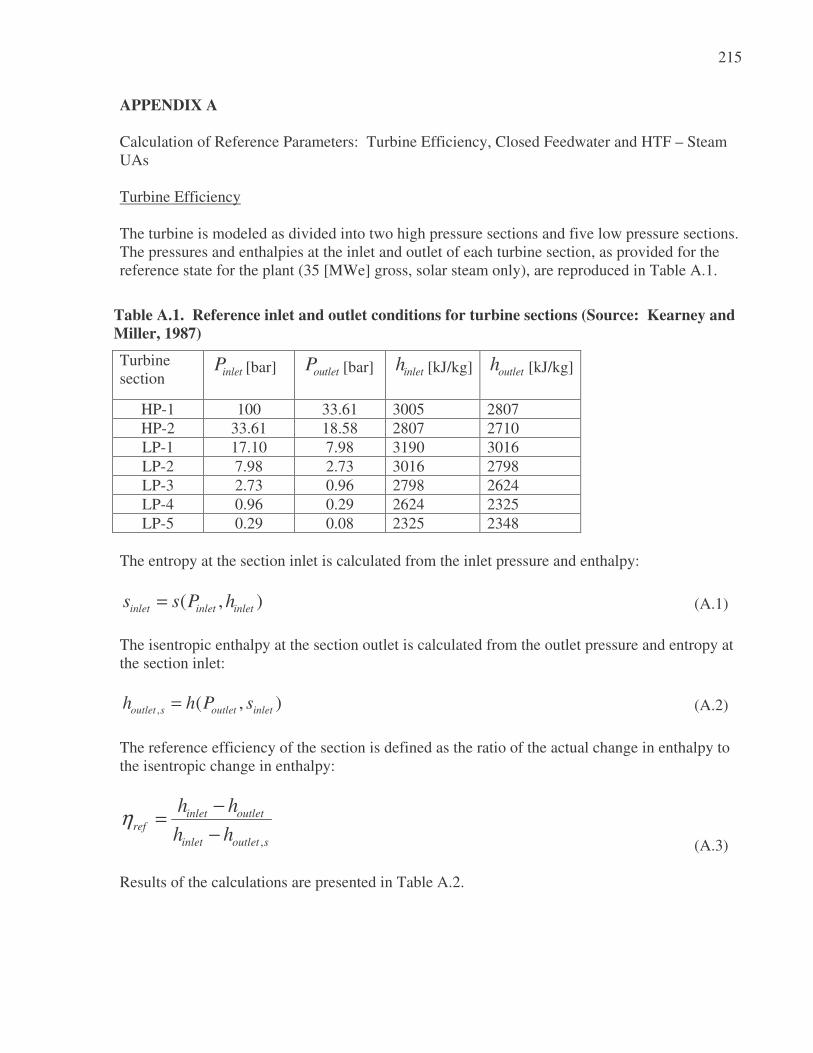
215

APPENDIX A

Calculation of Reference Parameters: Turbine Efficiency, Closed Feedwater and HTF – Steam UAs Turbine Efficiency The turbine is modeled as divided into two high pressure sections and five low pressure sections. The pressures and enthalpies at the inlet and outlet of each turbine section, as provided for the reference state for the plant (35 [MWe] gross, solar steam only), are reproduced in Table A.1.

Table A.1. Reference inlet and outlet conditions for turbine sections (Source: Kearney and

Miller, 1987)

Turbine section

inletP [bar] outletP [bar] inleth [kJ/kg] outleth [kJ/kg]

HP-1 100 33.61 3005 2807

HP-2 33.61 18.58 2807 2710

LP-1 17.10 7.98 3190 3016

LP-2 7.98 2.73 3016 2798

LP-3 2.73 0.96 2798 2624

LP-4 0.96 0.29 2624 2325

LP-5 0.29 0.08 2325 2348

The entropy at the section inlet is calculated from the inlet pressure and enthalpy:

( , )inlet inlet inlet

s s P h= (A.1)

The isentropic enthalpy at the section outlet is calculated from the outlet pressure and entropy at the section inlet:

, ( , )outlet s outlet inleth h P s= (A.2)

The reference efficiency of the section is defined as the ratio of the actual change in enthalpy to the isentropic change in enthalpy:

,

inlet outletref

inlet outlet s

h h

h hη

−=

− (A.3)

Results of the calculations are presented in Table A.2.

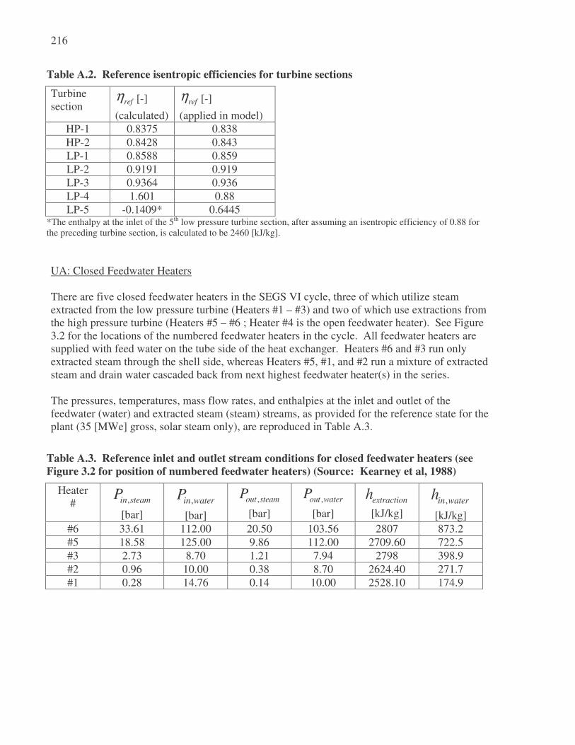
216

Table A.2. Reference isentropic efficiencies for turbine sections

Turbine section

refη [-]

(calculated)

refη [-]

(applied in model)

HP-1 0.8375 0.838

HP-2 0.8428 0.843

LP-1 0.8588 0.859

LP-2 0.9191 0.919

LP-3 0.9364 0.936

LP-4 1.601 0.88

LP-5 -0.1409* 0.6445 *The enthalpy at the inlet of the 5th low pressure turbine section, after assuming an isentropic efficiency of 0.88 for the preceding turbine section, is calculated to be 2460 [kJ/kg].

UA: Closed Feedwater Heaters There are five closed feedwater heaters in the SEGS VI cycle, three of which utilize steam extracted from the low pressure turbine (Heaters #1 – #3) and two of which use extractions from the high pressure turbine (Heaters #5 – #6 ; Heater #4 is the open feedwater heater). See Figure 3.2 for the locations of the numbered feedwater heaters in the cycle. All feedwater heaters are supplied with feed water on the tube side of the heat exchanger. Heaters #6 and #3 run only extracted steam through the shell side, whereas Heaters #5, #1, and #2 run a mixture of extracted steam and drain water cascaded back from next highest feedwater heater(s) in the series. The pressures, temperatures, mass flow rates, and enthalpies at the inlet and outlet of the feedwater (water) and extracted steam (steam) streams, as provided for the reference state for the plant (35 [MWe] gross, solar steam only), are reproduced in Table A.3.

Table A.3. Reference inlet and outlet stream conditions for closed feedwater heaters (see

Figure 3.2 for position of numbered feedwater heaters) (Source: Kearney et al, 1988)

Heater # ,in steamP

[bar]

,in waterP

[bar]

,out steamP

[bar]

,out waterP

[bar]

extractionh

[kJ/kg]

,in waterh

[kJ/kg]

#6 33.61 112.00 20.50 103.56 2807 873.2

#5 18.58 125.00 9.86 112.00 2709.60 722.5

#3 2.73 8.70 1.21 7.94 2798 398.9

#2 0.96 10.00 0.38 8.70 2624.40 271.7

#1 0.28 14.76 0.14 10.00 2528.10 174.9

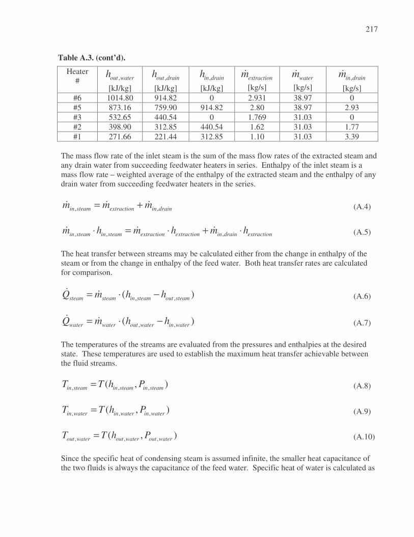
217

Table A.3. (cont’d).

Heater # ,out waterh

[kJ/kg]

,out drainh

[kJ/kg]

,in drainh

[kJ/kg]

extractionm�

[kg/s]

waterm�

[kg/s]

,in drainm�

[kg/s]

#6 1014.80 914.82 0 2.931 38.97 0

#5 873.16 759.90 914.82 2.80 38.97 2.93

#3 532.65 440.54 0 1.769 31.03 0

#2 398.90 312.85 440.54 1.62 31.03 1.77

#1 271.66 221.44 312.85 1.10 31.03 3.39

The mass flow rate of the inlet steam is the sum of the mass flow rates of the extracted steam and any drain water from succeeding feedwater heaters in series. Enthalpy of the inlet steam is a mass flow rate – weighted average of the enthalpy of the extracted steam and the enthalpy of any drain water from succeeding feedwater heaters in the series.

, ,in steam extraction in drainm m m= +� � � (A.4)

, , ,in steam in steam extraction extraction in drain extractionm h m h m h⋅ = ⋅ + ⋅� � � (A.5)

The heat transfer between streams may be calculated either from the change in enthalpy of the steam or from the change in enthalpy of the feed water. Both heat transfer rates are calculated for comparison.

, ,( )steam steam in steam out steamQ m h h= ⋅ −� � (A.6)

, ,( )water water out water in waterQ m h h= ⋅ −� � (A.7)

The temperatures of the streams are evaluated from the pressures and enthalpies at the desired state. These temperatures are used to establish the maximum heat transfer achievable between the fluid streams.

, , ,( , )in steam in steam in steamT T h P= (A.8)

, , ,( , )in water in water in waterT T h P= (A.9)

, , ,( , )out water out water out waterT T h P= (A.10)

Since the specific heat of condensing steam is assumed infinite, the smaller heat capacitance of the two fluids is always the capacitance of the feed water. Specific heat of water is calculated as

218

the difference in enthalpy of the feed water over the difference in temperature from inlet to outlet.

, ,

, ,

out water in water

water

out water in water

h hc

T T

−=

− (A.11)

The maximum heat transfer is determined from the capacitance rate of the feedwater multiplied by the difference in temperature between the two inlet streams:

max , ,( )water water in steam in waterQ m c T T= ⋅ −� � (A.12)

The ratio of actual heat transfer to maximum heat transfer establishes the reference effectiveness of the heat exchanger. The reference effectiveness is determined both using the heat transfer calculated on the steam side and using the heat transfer calculated on the feed water side.

max

steamsteam

Q

Qε =

�

� (A.13)

max

waterwater

Q

Qε =

�

� (A.14)

For heat exchangers in which one fluid undergoes a phase change, the effectiveness is related to the number of transfer units (NTU) through the following equation:

1 exp( )steam steam

NTUε = − − (A.15)

1 exp( )water waterNTUε = − − (A.16)

Finally, the ratio of the NTU to the heat capacitance of the feed water equals the reference UA of the heat exchanger:

steamsteam

water water

UANTU

m c=

⋅� (A.17)

waterwater

water water

UANTU

m c=

⋅� (A.18)

219

The pressure drop coefficient for the feed water is determined from the change in pressure of the feed water divided by the square of the feed water flow rate:

, ,

2

in water out water

water

water

P Pk

m

−=

� (A.19)

Results of the calculations are shown in Table A.4. refUA is a linear average of the UAs

calculated from the steam-side heat transfer and the water-side heat transfer.

Table A.4. Effectiveness and reference UA values for closed feedwater heaters

Heater # steamε steamUA

waterε waterUA refUA

#6 0.8344 318.3 0.8302 314 316

#5 0.8819 363.5 0.8756 354.7 360

#3 0.4448 77.2 0.4427 76.71 77

#2 0.9021 302.3 0.8968 295.5 300

#1 0.8452 241 0.8927 288.3 260

UA: HTF – Steam Heat Exchangers The pressures, temperatures, mass flow rates, and enthalpies at the inlet and outlet of each stream, as provided for the reference state for the plant (35 [MWe] gross, solar steam only), are reproduced in Table A.5.

Table A.5. Reference inlet and outlet stream conditions for HTF – steam heat exchangers (Source: Kearney and Miller, 1987)

Heat Exchanger ,in steamT ,in steamP ,in steam

h ,in steamx ,out steam

x ,out steamT ,out steamP

Preheater 234.83 103.56 ------ ------ 0 ------ 103.420

Steam Generation

------- 103.42 ------ 0 1 ------ 103.420

Superheater ------- 103.42 ------ 1 ------ 371 100.000

Reheater -------- 18.58 2709.6 ------ ------ 371 17.099

220

Table A.5. cont’d.

Heat Exchanger ,in HTFT ,out HTFT steamm�

[kg/s]

HTFm�

[kg/s]

Preheater 317.78 297.78 38.969 345.49

Steam Generation 377.22 317.78 38.969 345.49

Superheater 390.56 377.22 38.969 345.49

Reheater 390.56 294.00 33.034 50.90

Steam enthalpy at the inlet of the preheater is calculated from the given inlet temperature and pressure; enthalpies at the inlet and outlet of the steam generator are calculated assuming the inlet and outlet quality to the steam generator are 0 and 1, respectively. The temperature at the steam generator inlet and outlet is the saturation temperature at the specified steam generator pressure. The enthalpy of steam at the reheater inlet is calculated from the inlet enthalpy and pressure; temperature equals saturation temperature at the given inlet pressure. Outlet enthalpies are calculated from the outlet pressure and quality or outlet pressure and temperature, depending on which two values are given. The heat transfer between streams may be calculated either from the change in enthalpy of the feedwater/steam or from the change in enthalpy of the heat transfer fluid. Both heat transfer rates are calculated for comparison.

, ,( )steam steam in steam out steamQ m h h= ⋅ −� � (A.20)

, ,( )HTF HTF HTF in HTF out HTFQ m c T T= ⋅ −� � (A.21)

The specific heat of the heat transfer fluid is evaluated at the average temperature of the HTF in the heat exchanger.

, ,

2

in HTF out HTF

HTF HTF

T Tc c

+ =

(A.22)

The capacitance rate of each stream is the product of its mass flow rate and specific heat:

, ,

, ,

out steam in steam

C steam

out steam in steam

h hC m

T T

−= ⋅

−� (A.23)

H HTF HTFC m c= ⋅� (A.24)

The only exception to Equation A.23 occurs over the steam generator, in which case the specific heat of the boiling steam is assumed to be infinite.

221

The minimum and maximum heat capacitance rates of the two streams are identified, and the capacitance rate ratio is calculated:

min ( , )C H

C MIN C C= (A.24)

max ( , )C H

C MAX C C= (A.25)

min

max

r

CC

C= (A.26)

The maximum heat transfer is determined from the smaller capacitance rate of the two fluids multiplied by the difference in temperature between the two inlet streams:

max min , ,( )in HTF in steamQ C T T= −� (A.27)

The ratio of actual heat transfer to maximum heat transfer establishes the reference effectiveness of the heat exchanger. The reference effectiveness is calculated both using the heat transfer calculated on the steam side and using the heat transfer calculated on the heat transfer fluid side.

max

steamsteam

Q

Qε =

�

� (A.28)

max

HTFHTF

Q

Qε =

�

� (A.29)

For counterflow heat exchangers, the effectiveness is related to the number of transfer units (NTU) and capacitance ratio through the following equation:

( )

( )

1 exp 1

1 exp 1

r

r r

NTU C

C NTU C

− − ⋅ − ε =− ⋅ − ⋅ −

(A.30)

The exception to Equation A.30 occurs over the steam generator, where effectiveness is calculated according the Equation A.15. The ratio of the NTU to the heat capacitance of the feed water equals the reference UA of the heat exchanger:

222

min

steamsteam

UANTU

C= (A.31)

min

HTFHTF

UANTU

C= (A.32)

The pressure drop coefficient for the steam is determined from the change in pressure of the steam divided by the square of the steam mass flow rate:

, ,

2

in steam out steam

steam

steam

P Pk

m

−=

� (A.34)

Results of the calculations are shown in Table A.6. refUA is the UA used in the power cycle

model for the heat exchanger. It was assumed that the properties of steam were better known than those of the heat transfer fluid, for which it is not known what property data or assumptions were used in determining the reference temperatures. For this reason, the UAs calculated on the steam side were used in the power cycle model. The preheater model was written so as not to require a UA value; instead, the preheater model is written to calculate the outlet state of the working fluid as that of saturated liquid at the outlet pressure.

Table A.6. Effectiveness and reference UA values for closed feedwater heaters

HTFε HTFUA

steamε steamUA refUA

Preheater 0.9724 891.1 0.9481 724 -----

Steam Generator

0.9328 2371 0.9033 2051 2051

Superheater 0.8081 356.9 0.7462 292.5 292

Reheater 0.5844 149.1 0.8925 653.3 653

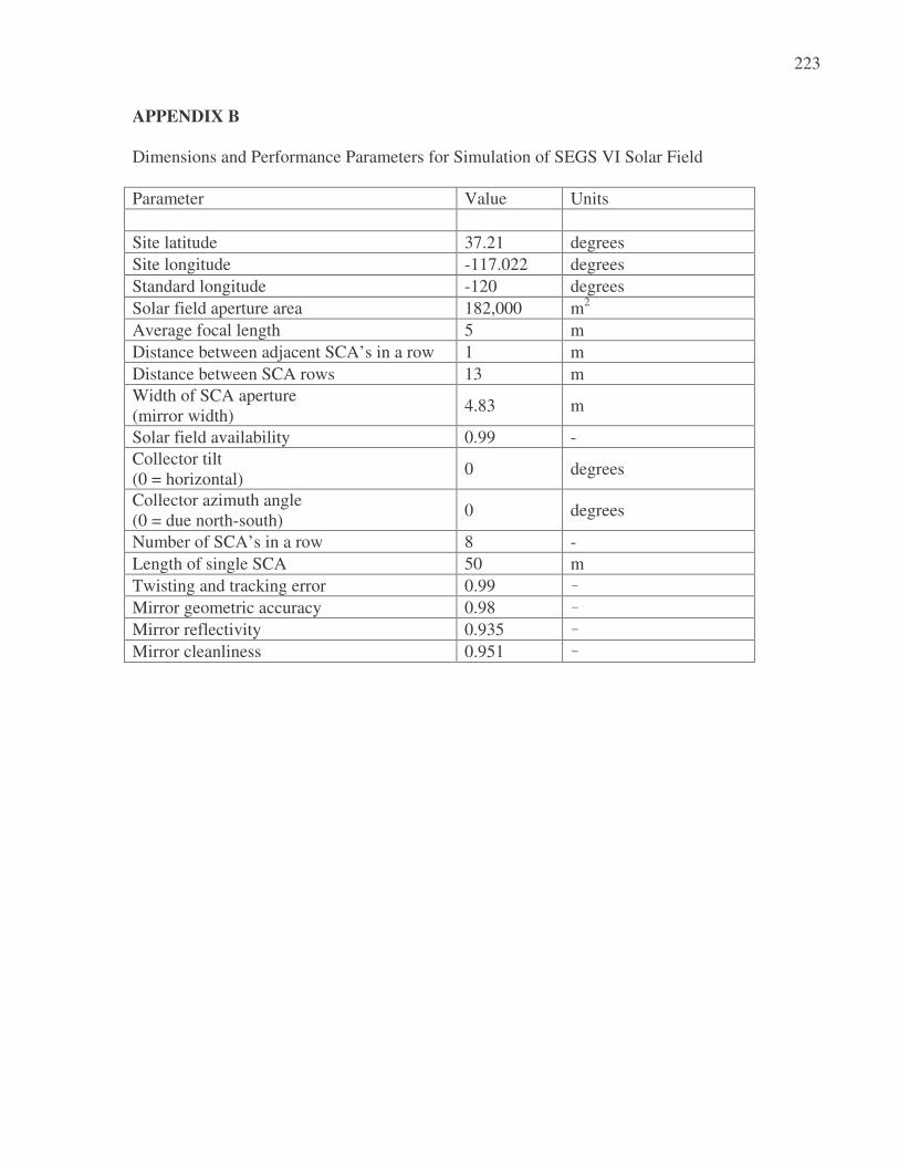
223

APPENDIX B Dimensions and Performance Parameters for Simulation of SEGS VI Solar Field

Parameter Value Units

Site latitude 37.21 degrees

Site longitude -117.022 degrees

Standard longitude -120 degrees

Solar field aperture area 182,000 m2

Average focal length 5 m

Distance between adjacent SCA’s in a row 1 m

Distance between SCA rows 13 m

Width of SCA aperture (mirror width)

4.83 m

Solar field availability 0.99 -

Collector tilt (0 = horizontal)

0 degrees

Collector azimuth angle (0 = due north-south)

0 degrees

Number of SCA’s in a row 8 -

Length of single SCA 50 m

Twisting and tracking error 0.99 -

Mirror geometric accuracy 0.98 -

Mirror reflectivity 0.935 -

Mirror cleanliness 0.951 -

224

APPENDIX C TRNSYS Listing: Type 805 (Solar Field Model) General Description Type 805 models a parabolic trough collector solar field. The incident radiation absorbed through the collector tubes is calculated as a function of direct normal insolation, incidence angle, incidence angle modifier, and other corrections for surface properties, shading, end losses, and solar collector field tracking/ focusing accuracy. Thermal losses from the collectors are modeled as a function of direct normal insolation and solar field temperatures at the inlet and outlet of the solar field; coefficients for the thermal loss equations are derived from an analytical heat transfer analysis and modeling program. (See Forristall.ees on the attached disk). Thermal losses from the piping leading to and from the solar field are also included. The model can operate in one of two modes. When SFMode = 1, the model is provided the volumetric flow rate of the solar field and returns the solar field outlet temperature. When SFMode = 2, the model is provided the desired solar field outlet temperature and returns the mass flow rate required to achieve the desired outlet temperature. Calculations for heat addition required to prevent the heat transfer fluid from freezing in the field at night and parasitic power requirements for the field are included in the model as well. Nomenclature

(0..3),1..na = coefficients for thermal heat loss as a function of temperature [-]

AntiFrPar = anti freeze pumping when field is circulated at night [MW]

(0..1),1..nb = coefficients for thermal heat loss as a function of direct normal insolation [-]

iBelShad = performance factor for losses due to shadows cast by metal bellows

HTFC Par = parasitics for pumping of cold heat transfer fluid (HTF at solar field inlet)

[MW]

HTFC ParPF = performance factor to adjust parasitics for pumping of cold heat transfer

fluid (HTF at solar field inlet) [-]

0...2HTFC ParF = coefficients of equation to adjust parasitics for pumping of cold heat transfer

fluid as a function of solar field load [-]

ColAz = azimuthal angle of orientation of collectors (0 = collector rows are oriented due north-south) [-]

ColTilt = tilt of collectors from horizontal (0 = collectors are parallel with ground) [degrees]

,1...Type nCol = type of collector (there is no internal numeric code for different collector

types; are collector type parameters are supplied by the user) [-]

,1...frac nCol = fraction of the solar field composed of the given type of collector [-]

225

DNI = direct normal insolation, per unit area [W/m2]

RowsDistance = distance between parallel rows of solar collector assemblies [m]

DSTadjust = adjustment to local time for Daylight Savings Time [hr]

EndLoss = performance factor; adjusts incident radiation for losses from the ends of the HCEs due to a non-zero angle of incidence [-]

iEnvTrans = transmissivity of HCE glass envelope [-]

FocalLength = average focal length of troughs in field [m]

1...nGeoAcc = geometric (focusing) accuracy associated with the collector type [-]

h = enthalpy of heat transfer fluid [kJ/kg]

fluidHTF = type of heat transfer fluid [-] (types are organized by numeric code:

1 – Nitrate salt 2 – Caloria HT 43 3 – Hitec XL 4 – Therminol VP-1 5 – Hitec 6 – Dowtherm Q 7 – Dowtherm RP)

,abs iHCE = HCE absorbtivity [-]

,dust iHCE = performance factor for level of dust accumulation on HCE [-]

,misc iHCE = miscellaneous performance factor for HCE absorbtivity losses [-]

,1...Type nHCE = type of HCE (types are organized by numeric code: 1 – UVAC Cermet,

vacuum intact, 2 – UVAC Cermet, air in annulus, 3 – UVAC Cermet, lost/broken envelope, 4 – UVAC Cermet, hydrogen in annulus) [-]

,1...frac nHCE = fraction of the solar field composed of the given type of HCE [-]

IAM = incidence angle modifier [-]

0...2IAMF = coefficients in incidence angle modifier equation [-]

K = modified incidence angle, as defined in Dudley et al (1994)

siteL = longitude of plant location [degrees]

standardL = longitude of standard meridian, off which local time zone is based [degrees]

HTFm� = mass flow rate of heat transfer fluid [kg/s]

,minHTFm� = minimum permissible mass flow rate in solar field [kg/s]

,maxHTFm� = maximum permissible mass flow rate in solar field [kg/s]

1...nMirRef = reflectivity of mirrors associated with the collector type [-]

1...nMirCln = cleanliness of mirrors associated with the collector type [-]

226

ShadowMode = mode for determining shadowing of solar field (0 = assume collectors are

tracking sun at all times, 1 = assume collector do not track sun until collector is less than half shaded) [m]

NumSCAs = number of solar collector assemblies in one row [-]

TypeNumHCE = number of “types” of HCEs found in the field (each type has an associated

set of surface and performance parameters, as well as its own coefficients for the receiver heat loss equation) [-]

TypeNumCol = number of “types” of collectors found in the field (each type has an

associated set of optical and performance parameters) [-]

absorbedQ� = thermal energy absorbed in the solar field, per unit solar field aperture area

[W/m2]

retainedQ� = thermal energy retained by the solar field, per unit solar field aperture area

[W/m2]

RecHl = receiver heat loss, per unit solar field aperture area [W/m2]

RowShadow = ratio of effective (unshaded) width of mirror aperture to actual mirror aperture width [-]

lengthSCA = length of a single solar collector assembly [m]

spacingSCA = spacing between solar collector assemblies (SCAs) in a row [m]

SFAvail = solar field availability – fraction of the solar field that is in operation [-]

AreaSF = total aperture area of mirrors in solar field [m2]

SFMode = solar field mode (1 = calculates outlet temperature based on mass flow rate, 2 = calculates mass flow rate to achieve set outlet temperature) [-]

SfPar = solar field LOC and motor parasitics [MW]

SfParPF = performance factor to adjust solar field LOC and motor parasitics [-]

SfPipeHl = thermal energy losses from piping leading to and from solar field, per unit

solar field aperture area [W/m2]

LatSite = latitude of plant location [degrees]

SolarAlt = solar altitude angle [degrees]

SolarAz = solar azimuth angle [degrees]

ambientT = ambient air temperature [C]

,minHTFT = minimum HTF temperature that must be maintained in the solar field to

prevent freezing [C]

,HTF inT = temperature of heat transfer fluid entering solar field [C]

,HTF outT = temperature of heat transfer fluid exiting solar field [C]

227

,out designT = desired solar field outlet temperature (also maximum temperature at solar

field outlet [m]

1...nTrkTwstEr = twisting and tracking error associated with the collector type [-]

HTFV� = volumetric flow rate of heat transfer fluid [m3/s]

effW = effective (unshaded) width of mirror aperture [m]

Width = width of mirror aperture [m]

WindSpeed = wind speed [m/s]

HCEη = efficiency of heat collection element [-]

fieldη = efficiency of solar field [-]

ρ = density of heat transfer fluid [kg/m3]

θ = angle of incidence between beam radiation and normal to collector surface [degrees]

Zθ = zenith angle [degrees]

Mathematical Description

The energy absorbed by the receivers is the product of the direct normal insolation, cosine of the angle of incidence, and performance factors correcting for mutual row shading, end losses, collector field and HCE surface properties, and solar field availability:

cos( )absorbed field HCEQ DNI IAM RowShadow EndLoss SFAvailθ η η= ⋅ ⋅ ⋅ ⋅ ⋅ ⋅ ⋅� (C.1)

The cosine of the incidence angle is calculated from Stine and Harrigan (1984):

2cos( ) 1 cos( ) cos( ) ( ) (1 cos( ))SolarAlt ColTilt ColTilt Cos SolarAlt SolarAz ColAzθ = − − − ⋅ ⋅ − − (C.2)

The incidence angle modifier is adapted from performance tests on an LS-2 collector conducted at Sandia National Laboratories (Dudley, 1994):

2

0 1 2cos( ) cos( )

IAM IAMF IAMF IAMFθ θ

θ θ= + ⋅ − ⋅

(C.3)

In this application, the incidence angle modifier is defined as

228

cos( )

KIAM

θ= (C.4)

RowShadow accounts for shading of parallel rows of collectors when the solar altitude angle is low, such as during early morning and late afternoon hours of operation. RowShadow is the ratio of the effective aperture width of the mirrors (the unshaded width of the mirrors) to the actual width of the mirrors.

cos( )

cos( )

eff Rows ZW Distance

RowShadowWidth Width

θ

θ= = ⋅

(C.5)

EndLoss accounts for reflective losses from the ends of a collector row due to a non-zero angle of incidence (Lippke, 1995).

tan( )1

Length

FocalLengthEndLoss

SCA

θ= −

(C.6)

The total collector field efficiency and HCE efficiency for the field are calculated as a weighted average of the performance of each type of collector or HCE in the field. The combined effects of optical and correction parameters for the heat collection element and collector field (mirror and tracking equipment) are accounted for in the HCE efficiency term, and collector efficiency

term, ηHCE and ηfield, respectively:

1

NumCol

field i i i i i

i

ColFrac TrkTwstErr GeoAcc MirRef MirClnη=

= ⋅ ⋅ ⋅ ⋅∑ (C.7)

1

NumHCE

HCE i i i i i i

i

HCEFrac HCEdust BelShad EnvTrans HCEabs HCEmiscη=

= ⋅ ⋅ ⋅ ⋅ ⋅∑ (C.8)

The heat loss from the receivers, per unit length trough [W/m], is calculated from:

229

,

1, 2,2 2 3 3

0, , , , , , ,

, ,

3, 1,4 4 3 3

, , 0, , , , ,

1 2

( ) ( ) ( )2 31( )

( ) ( ) ( )4 3

2

Field n

n n

n HTF out HTF in HTF out HTF in HTF out HTF in

HTF out HTF in

n n

HTF out HTF in n HTF out HTF in HTF out HTF in

HL HL HL

a aa T T T T T T

HLT T

a bT T DNI b T T T T

HL

= +

− + − + −=

−

− + − + −

=, ,( )HTF out HTF inT T−

(C.9)

,

1

NumHCETypesField n

n

n

HLRecHL HCEFrac

Width=

= ⋅∑ (C.10)

RecHL is the heat loss from the receiver tubes due to convection and radiation with the surroundings, in [W/m2]. HLfield is a term for the curve fit to the heat loss predicted by Forristall’s model as a function of the solar field inlet and exit temperatures; units are W/m (heat loss per unit length of HCE).

The solar field piping heat losses are calculated as a function of the difference between the average solar field temperature and the ambient air temperature (Price, 2005).

2 7 30.01693 0.0001683 6.78 10SfPipeHl T T T−= ∆ − ∆ + ⋅ ∆ (C.11)

where

, ,

2

HTF out HTF in

ambient

T TT T

+∆ = −

(C.12)

The difference between the energy absorbed by the HCEs and the losses from the field due to receiver heat losses and solar field piping heat losses is the energy collected by the field.

( )col absorbedQ Q RecHl SfPipeHl= − +� � (C.13)

230

In this model, the solar field outlet temperature is calculated from the outlet enthalpy, derived from an energy balance over the field as a function of the solar field inlet temperature, power collected by the field, and heat transfer fluid mass flow rate:

col area

HTF

Q SFh

m

⋅∆ =

�

� (C.14)

The inlet and outlet enthalpy of the heat transfer fluid are evaluated as a function of temperature obtained by integrating the specific heat of the fluid. Parasitic power requirements, when the solar field is collecting energy during the day, are calculated as a function of the energy absorbed by the solar field (Price, 2005).

2

0 1 2( )col colHTF HTF HTF HTF HTF

rated rated

SfTotPar SfPar SfParPF

Q QC Par C ParPF C ParF C ParF C ParF

Q Q

= ⋅

+ ⋅ + +

� �

� �

(C.15)

where

gross

rated

gross

WQ

η=�

� (C.16)

Parameters Number Name Dimension Unit Type Range Default

1 grossW� Power [MW] real [-inf;inf] 35

2 grossη Dimensionless [-] real [-inf;inf] 0.375

3 NumHCEType Dimensionless [-] real [-inf;inf] 4

4 NumColType Dimensionless [-] real [-inf;inf] 1

4+2n-1 ( )HCEType n Dimensionless [-] real [-inf;inf] 1

4+2n ( )HCEFrac n Dimensionless [-] real [-inf;inf] 1

4+2n+6i-5 ( )ColType i Dimensionless [-] real [-inf;inf] 1

4+2n+6i-4 ( )ColFrac i Dimensionless [-] real [-inf;inf] 1

4+2n+6i-3 ( )TrkTwstErr i Dimensionless [-] real [-inf;inf] 0.994

4+2n+6i-2 ( )GeoAcc i Dimensionless [-] real [-inf;inf] 0.98

4+2n+6i-1 ( )MirRef i Dimensionless [-] real [-inf;inf] 0.93

4+2n+6i ( )MirCln i Dimensionless [-] real [-inf;inf] 0.95

231

Inputs

Name Dimension Unit Type Range Default

1 ,HTF inT Temperature [C] real [-inf;inf] 80

2 DNI direct normal insolation, per unit area [W/mPower/Area [W/m2] real [-inf;inf] 0

3 ambientT latitude of plant location [degrees]Temperature [C] real [-inf;inf] 15

4 WndSpd Velocity [m/s] real [-inf;inf] 0

5 SFMode Dimensionless [-] real [-inf;inf] 0

6 HTFV� Flow Rate [m3/s] real [-inf;inf] 0.15

7 siteLat [deg] real [-inf;inf] 37

8 siteLong [deg] real [-inf;inf] -117.022

9 standardLong [deg] real [-inf;inf] -120

10 AreaSF Area [m2] real [-inf;inf] 182000

11 typeHTF Dimensionless [-] real [-inf;inf] 4

12 0IAMF Dimensionless [-] real [-inf;inf] 1

13 1IAMF Dimensionless [-] real [-inf;inf] 0.0506

14 2IAMF Dimensionless [-] real [-inf;inf] -0.1763

15 FocalLength Length [m] real [-inf;inf] 5

16 spacingSCA Length [m] real [-inf;inf] 5

17 RowsDistance Length [m] real [-inf;inf] 5

18 Width Length [m] real [-inf;inf] 4.83

19 SFAvail Dimensionless [-] real [-inf;inf] 0.99

20 ColTilt [deg] real [-inf;inf] 0

21 ColAz [deg] real [-inf;inf] 0

22 NumSCAs Dimensionless [-] real [-inf;inf] 8

23 lengthSCA Length [m] real [-inf;inf] 50

24 ,minHTFT Temperature [C] real [-inf;inf] 50

25 SfPar Dimensionless [-] real [-inf;inf] 0.1357

26 SfParPF Dimensionless [-] real [-inf;inf] 1

232

27 HTFC Par Dimensionless [-] real [-inf;inf] 5.3664

28 HTFC ParPF Dimensionless [-] real [-inf;inf] 1

29 0HTFC ParF Dimensionless [-] real [-inf;inf] -0.036

30 1HTFC ParF Dimensionless [-] real [-inf;inf] 0.242

31 2HTFC ParF Dimensionless [-] real [-inf;inf] 0.794

32 AntiFrPar Dimensionless [-] real [-inf;inf] 0.5366

33 DSTadjust Time [hr] real [-inf;inf] 0

34 ShadowMode Dimensionless [-] real [-inf;inf] 1

35 ,out designT Temperature [C] real [-inf;inf] 400

36 ,minHTFm� Flow Rate [kg/s] real [-inf;inf] 50

37 ,maxHTFm� Flow Rate [kg/s] real [-inf;inf] 550

Outputs


1 ,HTF outT Temperature [C] real [-inf;inf] 80

2 absorbedQ� Power/Area [W/m2] real [-inf;inf] 0

3 RecHL Power/Area [W/m2] real [-inf;inf] 0

4 SfPipeHL Power/Area [W/m2] real [-inf;inf] 0

5 collectedQ� Power/Area [W/m2] real [-inf;inf] 0

6 IAM Dimensionless [-] real [-inf;inf] 0

7 FreezeProtQ� Power [MW] real [-inf;inf] 0

8 SFQ� Power/Area [MW] real [-inf;inf] 0

9 HTFm� Flow Rate [kg/hr] real [-inf;inf] 100

10 SFTotPar Power [MW] real [-inf;inf] 0

11 fieldη Dimensionless [-] real [-inf;inf] 0

12 EndLoss Dimensionless [-] real [-inf;inf] 0

13 RowShadow Dimensionless [-] real [-inf;inf] 0

14 HCEη Dimensionless [-] real [-inf;inf] 0

233

Information Flow Diagram

Inputs: 1. ,HTF inT 11. typeHTF 21. ColAz 31. 2HTFC ParF

2. DNI 12. 0IAMF 22. NumSCAs 32. AntiFrPar

3. ambientT 13. 1IAMF 23. lengthSCA 33. DSTadjust

4. WndSpd 14. 2IAMF 24. ,minHTFT 34. ShadowMode

5. SFMode 15. FocalLength 25. SfPar 35. ,out designT

6. HTFV� 16. spacingSCA 26. SfParPF 36. ,minHTF

m�

7. siteLat 17. RowsDistance 27. HTFC Par 37. ,maxHTFm�

8. siteLong 18. Width 28. HTFC ParPF

9. standardLong 19. SFAvail 29. 0HTFC ParF

10. AreaSF 20. ColTilt 30. 1HTFC ParF

,HTF outT

INPUTS (see Inputs table below)

TYPE 805 Solar Field Model

7… 9… 11… 37 13… 15… 17… 19… 21… 23… 31… 33… 35… 25… 27… 29… 1… 3… 5…

1 2 3 4 5 6 7 8 9 10 11 12 13 14

absorbedQ�

RecHL

SfPipeHL

collectedQ� fieldη FreezeProtQ�

IAM SFQ�

HTFm�

SFTotPar EndLoss

RowShadow

HCEη

234

Parameters: 1. grossW�

2. grossη

3. NumHCEType

4. NumColType

4+2n-1. ( )HCEType n

4+2n. ( )HCEFrac n

4+2n+6i-5. ( )ColType i

4+2n+6i-4. ( )ColFrac i

4+2n+6i-3. ( )TrkTwstErr i

4+2n+6i-2. ( )GeoAcc i

4+2n+6i-1. ( )MirRef i

4+2n+6i. ( )MirCln i

235

APPENDIX D TRNSYS Listing: Type 811 (Power Cycle Model) General Description Type 811 models a Rankine steam power cycle and is written to interface with a concentrating solar power thermal energy collection system, such as a parabolic trough solar field (Type 805) or storage tank. Type 811 is designed for use in conjunction with an external thermodynamic power cycle model, such as SEGSVI.ees (included on the attached disk). The steady-state power cycle performance must be regressed in terms of the heat transfer fluid temperature, heat transfer fluid mass flow rate, and condensing pressure; coefficients of the linear regression equations are taken from the external program and supplied as inputs to Type 811. The component calculates the gross power output and the temperature of the heat transfer fluid exiting the power block, as well as the enthalpy and mass flow rate of steam at the entrance of the steam condenser. If the energy input to the heat transfer fluid is insufficient to produce power, the component sets all outputs to default values. Nomenclature

0...9a = coefficients for linear regression equation for gross power output [-]

0...9b = coefficients for linear regression equation for temperature of heat transfer

fluid exiting power block [-]

0...9c = coefficients for linear regression equation for mass flow rate of steam

entering steam condenser [-]

0...9d = coefficients for linear regression equation for enthalpy of steam entering

steam condenser [-]

steamh = enthalpy of steam entering steam condenser [kJ/kg]

HTFm� = mass flow rate of heat transfer fluid [kg/hr]

steamm� = mass flow rate of condensing steam [kg/hr]

P = condensing pressure of steam [bar]

,HTF inT = temperature of heat transfer fluid entering power cycle [C]

,HTF outT = temperature of heat transfer fluid exiting power cycle [C]

absorbedQ� = thermal energy absorbed in the solar field [W/m2]

grossW� = thermal energy absorbed in the solar field [W/m2]

236

Mathematical Description All outputs from the component are calculated in terms of heat transfer fluid temperature [C], heat transfer fluid flow rate [kg/s], and condensing pressure [bar]. Coefficients of the equations are obtained from linear regression curve fits, provided by an external model for the power cycle, in terms of the dependent variables shown, with units for the dependent variables as listed above.

2 2

0 1 2 3 4 5 ,

2

6 , 7 8 , 9 ,

gross HTF HTF HTF in

HTF in HTF HTF HTF in HTF in

W a a m a m a P a P a T

a T a m P a m T a P T

= + ⋅ + ⋅ + ⋅ + ⋅ + ⋅

+ ⋅ + ⋅ ⋅ + ⋅ ⋅ + ⋅ ⋅

� � �

� � (D.1)

2 2

, 0 1 2 3 4 5 ,

2

6 , 7 8 , 9 ,

HTF out HTF HTF HTF in


T b b m b m b P b P b T

b T b m P b m T b P T

= + ⋅ + ⋅ + ⋅ + ⋅ + ⋅

+ ⋅ + ⋅ ⋅ + ⋅ ⋅ + ⋅ ⋅

� �

� � (D.2)

2 2

0 1 2 3 4 5 ,

2

6 , 7 8 , 9 ,

steam HTF HTF HTF in


m c c m c m c P c P c T

c T c m P c m T c P T

= + ⋅ + ⋅ + ⋅ + ⋅ + ⋅

+ ⋅ + ⋅ ⋅ + ⋅ ⋅ + ⋅ ⋅

� � �

� � (D.3)

2 2

0 1 2 3 4 5 ,

2

6 , 7 8 , 9 ,

steam HTF HTF HTF in


h d d m d m d P d P d T

d T d m P d m T d P T

= + ⋅ + ⋅ + ⋅ + ⋅ + ⋅

+ ⋅ + ⋅ ⋅ + ⋅ ⋅ + ⋅ ⋅

� �

� � (D.4)

If the energy absorbed by the solar field is insufficient to produce power (<60 [W/m2]), the component sets the gross power output to 0 and the heat transfer fluid temperature at the outlet to the heat transfer fluid temperature at the inlet. Enthalpy and mass flow rate of steam entering the steam condenser are set to default values.

Inputs


1 ,HTF inT Temperature [C] real [-inf;inf] 140

2 HTFm� Flow rate [kg/hr] real [-inf;inf] 180000

3 P Pressure [bar] real [-inf;inf] 0.08

4 0a Dimensionless [-] real [-inf;inf] 48.00749

5 1a Dimensionless [-] real [-inf;inf] -0.07447251



8 4a Dimensionless [-] real [-inf;inf] 0

237






14 0b Dimensionless [-] real [-inf;inf] -8.50750675

15 1b Dimensionless [-] real [-inf;inf] 0.0716221364


17 3b Dimensionless [-] real [-inf;inf] 0







24 0c Dimensionless [-] real [-inf;inf] 31.17463

25 1c Dimensionless [-] real [-inf;inf] -0.05197693


27 3c Dimensionless [-] real [-inf;inf] 0







34 0d Dimensionless [-] real [-inf;inf] 2017.243

35 1d Dimensionless [-] real [-inf;inf] -0.9401352

238









44 absorbed

Q� Power/Area [W/m2] real [-inf;inf] 0

Outputs


1 grossW� Power [MW] real [-inf;inf] 0

2 ,HTF outT Temperature [C] real [-inf;inf] 80

3 steamm� Flow Rate [kg/s] real [-inf;inf] 32

4 steamh Enthalpy [kJ/kg] real [-inf;inf] 2025

5 HTFm� Flow Rate [kg/s] real [-inf;inf] 400

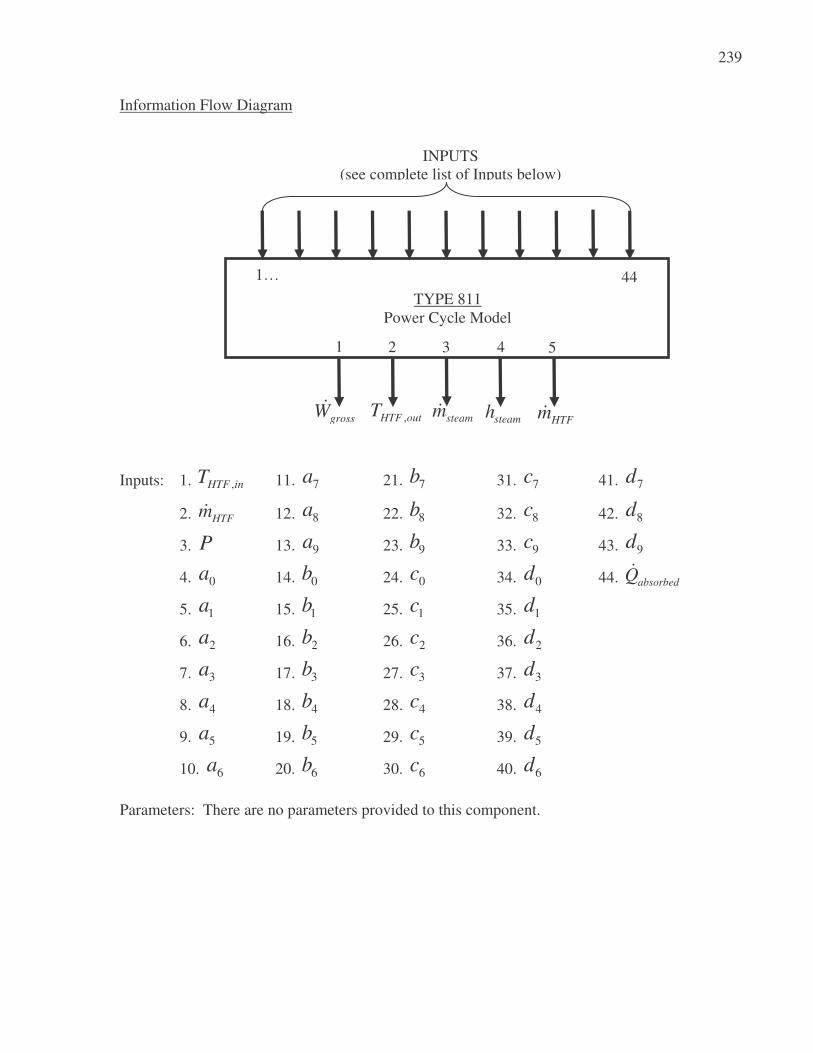
239


Inputs: 1. ,HTF inT 11. 7a 21. 7b 31. 7c 41. 7d

2. HTFm� 12. 8a 22. 8b 32. 8c 42. 8d

3. P 13. 9a 23. 9b 33. 9c 43. 9d

4. 0a 14. 0b 24. 0c 34. 0d 44. absorbedQ�

5. 1a 15. 1b 25. 1c 35. 1d

6. 2a 16. 2b 26. 2c 36. 2d

7. 3a 17. 3b 27. 3c 37. 3d

8. 4a 18. 4b 28. 4c 38. 4d

9. 5a 19. 5b 29. 5c 39. 5d

10. 6a 20. 6b 30. 6c 40. 6d

Parameters: There are no parameters provided to this component.

grossW�

TYPE 811 Power Cycle Model

1 2 3 4

INPUTS (see complete list of Inputs below)

1… 44

,HTF outT steamm� steamh HTFm�

5

240

APPENDIX E TRNSYS Listing: Type 816 (Steam Condenser Model) General Description Type 816 models the performance of a horizontal shell and tube steam condenser, in which steam condenses on the shell side of the exchanger and cold condenser water circulates through the tubes. The condensed steam exits the condenser as saturated liquid. The model is supplied with the enthalpy and mass flow rate of the entering steam, as well as the mass flow rate and temperature of the entering condenser water. The overall heat transfer conductance-area product (UA) at a reference condenser water flow rate is provided as a parameter to the model. The model uses an effectiveness-NTU relationship to predict the condensing pressure (and corresponding condensing temperature) of the steam. The temperature of the condenser water at the condenser outlet is determined from the model as well. The steam condenser is designed such that it can operate in conjunction with a solar field; if there is not sufficient energy absorbed in the solar field to produce power, the outputs are set to default values. Nomenclature

waterc = specific heat of water [kJ/kg-K]

,steam inh = enthalpy of steam entering steam condenser [kJ/kg]

,steam outh = enthalpy of steam exiting steam condenser [kJ/kg]

steamm� = mass flow rate of condensing steam [kg/hr]

waterm� = mass flow rate of condenser water [kg/hr]

,water REFm� = mass flow rate of condenser water at which reference UA is calculated

[kg/hr]

condenserNTU = number of transfer units for condenser [-]

condenseP = condensing pressure of steam [bar]

condenseT = condensing temperature of steam [C]

,water inT = temperature of condenser water at condenser inlet [C]

,water outT = temperature of condenser water at condenser outlet [C]

condenserUA = overall heat transfer conductance-area product for condenser [kW/K]

,condenser REFUA = reference overall heat transfer conductance-area product for condenser

[kW/K]

absorbedQ� = thermal energy absorbed in the solar field [W/m2]

241

condenserQ� = heat transfer from condensing steam to condenser water [kW]

,maxcondenserQ� = maximum heat transfer from steam to condenser water [kW]

condenserε = effectiveness of condenser [-]

Mathematical Description The UA of the condenser at the provided condenser water flow rate is calculated from the UA provided at the reference cooling water flow rate, multiplied by the ratio of the condenser water flow rate to the reference condenser water flow rate raised to the 0.8 power:

0.8

,

,

watercondenser condenser REF

water REF

mUA UA

m

=

�

� (E.1)

The UA of the condenser determines the number of transfer units (NTU) and effectiveness of the condenser:

condensercondenser

water water

UANTU

m c=

⋅� (E.2)

1 exp( )condenser condenserNTUε = − − (E.3)

The specific heat of the condenser water, as well as the specific heat of the condensed steam (saturated liquid), are both assumed constant. The enthalpy of the condenser water at the condenser water inlet temperature is used as an initial guess value for the exit enthalpy of the condensed steam. The condensing temperature is determined from the enthalpy guess value and the specific heat of the condensed steam:

,steam out

condense

water

hT

c= (E.4)

The heat transfer between streams, as well as the maximum heat transfer possible between streams, are calculated based on this condensing temperature:

, ,( )condenser steam steam in steam outQ m h h= −� � (E.5)

,max ,( )condenser water water condense water inQ m c T T= ⋅ −� � (E.6)

The effectiveness of the heat exchanger will equal the ratio of the actual heat transfer between streams (Equation E.5) to the maximum possible heat transfer between streams (Equation E.6).

242

,max

condensercondenser

condenser

Q

Qε =

�

� (E.7)

If the effectiveness of the condenser calculated from Equation E.7 does not match the effectiveness calculated from Equation E.3, the guess value for the exit enthalpy of the condensed steam is increased by 40 [kJ/kg], and Equations E.4 through E.7 are repeated. This iteration continues until the effectiveness of the condenser from Equation E.7 matches the effectiveness from Equation E.3. The condensing pressure is equal to the saturation pressure at the condensing temperature. The exit temperature of the cooling water is determined from the heat transfer between streams, assuming constant specific heat for the condenser water:

, ,condenser

water out water in

water water

QT T

m c= +

⋅

�

� (E.8)

The component is designed to operate in conjuction with a solar field. If the solar field has not absorbed a sufficient amount of energy to produce power, the component sets the condensing pressure and cooling water outlet temperature to 0.04 [bar] and 20 [°C], respectively.

Parameters


1 waterc Specific heat [kJ/kg-K] real [-inf;inf] 4.18

2 ,water REFm� Flow rate [kg/s] real [-inf;inf] 1500

3 ,condenser REFUA UA [kW/K] real [-inf;inf] 3600

Inputs


1 ,steam inh Enthalpy [kJ/kg] real [-inf;inf] 2500

2 steamm� Flow rate [kg/s] real [-inf;inf] 31.5

3 waterm� Flow rate [kg/hr] real [-inf;inf] 5400000

4 ,water inT Temperature [C] real [-inf;inf] 25

5 absorbedQ� Power /Area [W/m2] real [-inf;inf] 0

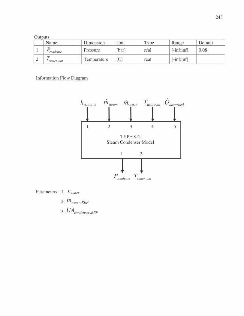
243

Outputs


1 condenseP Pressure [bar] real [-inf;inf] 0.08

2 ,water outT Temperature [C] real [-inf;inf]


Parameters: 1. waterc

2. ,water REFm�

3. ,condenser REFUA

condenseP

,steam inh

TYPE 812 Steam Condenser Model

1 2

1 2 3 4 5

steamm�

,water outT

waterm�

,water inT absorbedQ�

244

APPENDIX F

Contents of Enclosed CD: Modeling Files, Plant Data, and Other Resources Plant data 2004 – 2005

This folder contains the following files for all available days from January 1, 2004 through August 9, 2005. Files are named with the name or numerical designation for the system first, followed by the day number and the last two digits of the year. For example, ‘S6BLR.162.05.csv’ is the SEGS VI boiler data file for Day 162 (June 11) of the year 2005. Also, some 2004 files have ‘03’ appended to the end of the file name, i.e. ‘S6BLR’ is also called ‘S6BLR03’ for some days of the year in 2004. All data are recorded at 5-minute intervals between 5:00 AM and 8:30 PM unless otherwise noted. File Name: Description: S6BLR.csv – SEGS VI boiler data S6HTF.csv – SEGS VI heat transfer fluid data S6HXA.csv – SEGS VI heat exchanger data, Train A S6HXB.csv – SEGS VI heat exchanger data, Train B S6TUR.csv – SEGS VI turbine inlet/outlet data; also contains cooling water

inlet/outlet flow rates, as well as gross and parasitic power S602.csv – SEGS VI hourly averages for turbine data S604.csv – SEGS VI hourly averages, heat exchangers Trains A and B S605.csv – SEGS VI hourly averages, boiler data S608.csv – SEGS VI hourly averages, feedwater heaters #1 - #3 S609.csv – SEGS VI hourly averages, feedwater heaters #4 - #6 S701.csv – SEGS VII hourly performance averages; includes hourly average

weather readings and gross and parasitic power S6010.csv – (unclear; data columns not labeled) S6015.csv – SEGS VI boiler combustion data (at one-minute intervals) S6017.csv – SEGS VI reheater inlet pressure and temperature data, Trains A and B

(from 6:00 AM through noon) weather2004-1.csv - Kramer Junction weather station data at 5-minute intervals, for 24

hours/day, from January 1 to June 30, 2004 weather2004-2.csv - Kramer Junction weather station data at 5-minute intervals, for 24

hours/day, from July 1 to December 31, 2004 weather2005.csv - Kramer Junction weather station data at 5-minute intervals, for 24

hours/day, from January 1 to August 9, 2005

245

Plant data 1998

This folder contains the following files for twenty-one (21) days in 1998 in which it is believed the plant operated in solar-only mode. Files are named with the name for the system first, followed by the day number. The solar-only days included in this folder are:

Day 101 – 105 Day 109 – 110 Day 170 – 174 Day 262 – 263 Day 344 – 350

File Name: Description: S6HTF98.csv – SEGS VI heat transfer fluid data S6HXA98.csv – SEGS VI heat exchanger data, Train A S6HXB98.csv – SEGS VI heat exchanger data, Train B S6TUR98.csv – SEGS VI turbine inlet/outlet data; also contains cooling water

inlet/outlet flow rates, as well as gross and parasitic power TRNSYS Types and Models

This folder contains a sample .dck file for simulation of the comprehensive system model in TRNSYS, as well as all input files and non-standard TRNSYS components required to run the model. File Name: Description: SEGSVISystem.dck Deck file for the comprehensive model simulation of the SEGS plant.

*NOTE: this .dck was created and written directly in the .dck file, without use of the TRNSYS Simulation Studio. Attempting to view the file in the Studio window might not work very well.

Type805.f90 Fortran code for the solar field model Type811.f90 Fortran code for the power cycle model (polynomial equations for gross

power, heat transfer fluid temperature at heat exchanger outlet, and enthalpy and mass steam flow to the condenser as a function of heat transfer fluid inlet temperature and flow rate and condensing pressure)

Type806.f90 Fortran code for the steam condenser model *NOTE: None of the Types created for this project currently have proformas written for them.

246

EES files

All EES code created for modeling the power cycle and the comprehensive system is contained in this folder. The HCE heat transfer analysis program written by Forristall (2003) is included in this folder as well. File Name: Description: SEGSVI.ees This is the “user-friendly” version of the power cycle model. It includes

diagram windows for user inputs. This file contains the power cycle only. SEGSComplete.ees This file contains code for the power cycle, solar field, and heat rejection

system, all coupled in one program. This file was used for uncertainty analysis of the comprehensive model.

Forristall.ees The HCE heat transfer analysis and modeling program written by Forristall (last updated 03/19/05).

Thesis and Powerpoints

Contains the Masters thesis, in both .doc and .pdf format, and Powerpoint presentations on SEGS VI created for Solar Energy Laboratory presentations, other class presentations, and the thesis defense. Other Resources

Contains journal articles, powerpoint presentations, and other supplemental information.

File Name: Description: Lippke.pdf “Simulation of the Part Load Behavior of a 30MWe SEGS Plant” Conradie.pdf “Performance Evaluation of Dry-Cooling Systems for Power Plant

Applications.” Forristall.pdf “Heat Transfer Analysis and Modeling of a Parabolic Trough Solar

Receiver Implemented in Engineering Equation Solver.” KJC.ppt “Kramer SEGS Facility Solar Electric Generating Systems III through

VII” Photos

Contains photographs taken by Angela Patnode at the SEGS III-VII (Kramer Junction) facility.

247

References Ashcroft (Website). “Ashcroft Products Quick Guides: Ashcroft Gauges – Digital Pressure

Gauges.” Available at http://www.ashcroft.com/products/qg.cfm?qg=gauges&sub=22. Last accessed December 12, 2005.

Bartlett, Robert L. Steam Turbine Performance and Economics. New York: McGraw-Hill,

1958. Braun, J. E. , Klein, S. A., and Mitchell, J. B. “Effectiveness Models for Cooling Tower and

Cooling Coils”. ASHRAE Transactions, 95, Part II, 164 (1989). Cohen, Gilbert E., Kearney, David W., and Kolb, Gregory J. Final Report on the Operation and

Maintenance Improvement Program for Concentrating Solar Power Plants. Sandia National Laboratories, SAND 99-1290. June 1999.

Conradie, A.E., and Kroger, D. G. “Performance Evaluation of Dry-Cooling Systems for Power

Plant Applications.” Applied Thermal Engineering, Vol. 16, No.3, pp 213 – 232. May 1995. Dudley, V., Kolb, G.J., Mahoney, A.R., Mancini, T.R., Matthews, C.W., Sloan, M., and

Kearney, D. Test Results: SEGS LS-2 Solar Collector. Sandia National Laboratories, SAND94-1884. December 1994.

Duffie, John A., and Beckman, William A. Solar Engineering of Thermal Processes. 2nd

edition. New York: John Wiley and Sons, Inc., 1991.

Engineering Equation Solver (EES). Middleton, WI: F-Chart Software, 2005. Available at http://www.fchart.com.

El-Wakil, M. M. Powerplant Technology. New York: McGraw-Hill, Inc., 1984. Emco (Website). “Turbo-Bar Insertion Turbine Flow Meter: Specifications.” Available at

http://www.emcoflow.com/em_prods/Turbo_Bar.aspx#specifications. Last accessed December 12, 2005.

Emco (Website). “Sono-Trak Doppler Ultrasonic: Specifications” Available at

http://www.emcoflow.com/em_prods/Sono_Trak_Doppler.aspx. Last accessed December 12, 2005.

Forristall, Russell. “Heat Transfer Analysis and Modeling of a Parabolic Trough Solar Receiver

Implemented in Engineering Equation Solver.” National Renewable Energy Laboratory, NREL/TP-550-34169. October 2003.

Gummo, Carin. personal communication. January 3, 2006.

248

Incropera, Frank P., and DeWitt, David P. Fundamentals of Heat and Mass Transfer. 5th edition. New York: John Wiley and Sons, Inc., 2002.

Iqbal, M. An Introduction to Solar Radiation. Ontario: Academic Press Canada, 1983.

Jones, Scott A., Pitz-Paal, R., Schwarzboezl, P., Blair, N., and Cable, R. TRNSYS Modeling of the SEGS VI Parabolic Trough Solar Electric Generating System. Proceedings of Solar Forum 2001, Washington, D.C. April 2001.

Kearney, David W., and Miller, Charles E. SEGS VI: Technical Evaluation of Project Feasibility. Submitted to Luz Solar Partners VI. January 1988.

KJC Operating Company (Powerpoint Presentation). “Kramer SEGS Facility Solar Electric

Generating Systems III through VII”. Last accessed October 20, 2004. Lippke, Frank. “Simulation of the Part Load Behavior of a 30MWe SEGS Plant.” Prepared for

Sandia National Laboratories, Albuquerque, NM, SAND95-1293. June 1995. Moran, Michael J, and Shapiro, Howard N. Fundamentals of Engineering Thermodynamics. 4th

Edition. John Wiley and Sons, Inc. 2000. Omega (Website). “Thermocouple Tolerances: American Limits of Error ASTM E230-ANSI

MC 96.1.” Available at http://www.omega.com/toc_asp/frameset.html?book=Temperature&file=TC_GEN_SPECS_REF. Last accessed December 12, 2005.

Price, Henry, and Kearney, David. Reducing the Cost of Energy from Parabolic Trough Solar

Power Plants. National Renewable Energy Laboratory, NREL/CP-550-33208. January 2003.

Price, Henry (Microsoft Excel program). Excelergy. Last updated 2005. Price, Henry. personal communication. August, 2005. Rosemount (Website). “Rosemount Compact Orifice Flowmeter Series: Product Data Sheet.”

Available at http://www.emersonprocess.com/rosemount/document/pds/4810b00n.pdf. Last accessed December 12, 2005.

SEGS VI Engineering Handbook. Vol. I – III. Prepared by Luz Industries. March, 1986. SEGS VI and VII Operations Manual. Rev 1. June, 1989. SEGS VI Instrument Index. Prepared by Ludan Engineering Co., Ltd. September 1988.

249

Solel UVAC (Website). “Solel #5 – the Only Proven and Cost Effective Parabolic Trough.” Available at http://solel.com/products/pgeneration/tkey_fields/. Last accessed December 14, 2005.

Stine, William B., and Harrigan, Raymond W. Solar Energy Fundamentals and Design, with

Computer Applications. John Wiley & Sons, Inc., 1985. Stodola, A., and Loewenstein, Louis C. Steam and Gas Turbines. Volume I. New York:

McGraw-Hill Book Company, 1945. Stuetzle, Thorsten A. Automatic Control of the 30MWe SEGS VI Parabolic Trough Plant.

Master’s Thesis, Department of Mechanical Engineering, University of Wisconsin – Madison. 2002.

TRNSYS – A Transient System Simulation Program. Madison, WI: University of Wisconsin-

Madison Solar Energy Laboratory. Available at http://sel.me.wisc.edu/trnsys/. University of Oregon Solar Radiation Monitoring Laboratory (Website). “Eppley Normal

Incident Pyrheliometer.” Available at http://solardat.uoregon.edu/EppleyNIP.html. Last accessed December 12, 2005.

Documents

Simulation and Performance Evaluation of Parabolic Trough