1

Simulation and control of direct driven permanent magnet synchronous generator (PMSG)

Paul Deglaire, Sandra Eriksson and Andreas Solum Division for electricity and lightning research

Uppsala University Supervisor: Ian Norheim

Local supervisor: Hans Bernhoff ********************************************************************* Nomenclature All values are p.u. values, unless other units are explicitly specified. Subscripts 1) q-d axis definition : see slide 25 in [1]. 2) s is relative to the stator voltage and currents. r is relative to the rotor. c indicates values flowing through the grid side converter. ex indicates values at the grid. Hence the currents flowing into the stator side converter will be iqs and ids in the d-q frame in p.u.

sP is the active power delivered at the stator terminal.

sQ is the reactive power delivered at the stator terminal. 22

sss QPS += apparent power. Generator electrical parameters fψ permanent magnet flux.

qsψ , dsψ flux through the stator in the q and d directions. θ load angle in rad, which is the phase angle between the no-load voltage and the load voltage of the permanent magnet generator.

eT electromechanical torque produced by the generator. qsL q-axis stator inductance.

dsL d-axis stator inductance. R stator resistance.

eω electrical frequency at the stator side. reω rated electrical frequency at the stator side in rad/s.

2

Wind turbine aerodynamic and mechanical parameters ρ density of air in kg/m3. PoptC maximum power efficiency at optimum tip speed ratio.

optλ tip speed ratio assumed constant to obtain PoptC . V wind speed in m/s. r turbine radius in m. mT torque produced by the turbine at a given wind speed.

refP reference power delivered to the generator assuming that the turbine is

producing maximum power at a given rω rotor speed.

ratedS rated power of the wind turbine at optimum wind speed and optimum tip speed ratio in Watts.

rω mechanical speed of the turbine. cutiω cut in mechanical speed of the turbine. ratedω rated mechanical speed of the turbine. rrω rated rotational speed of the turbine in rad/s . H: turbine plus shaft inertia normalized constant in seconds. DC link bus dU DC link voltage. C DC link capacitance. Grid Uex grid voltage. Xt grid side inductance.

α phase angle between cu and Uex. Chosen values for our system The chosen values for our system are presented in Appendix 1. Introduction The aim of this project is to make a dynamic power system simulation of a PMSG with a full scale converter as interface to the grid. This is to be done by establishing a SIMULINK model for the PMSG and to test the model with suitable simulations. Four control systems are to be implemented. These should control the electrical frequency for optimum efficiency, the reactive power exchange between the stator and the converter, the reactive power exchange with the grid and the DC-voltage level. All currents and voltages are represented in the d-q reference frame and all parameters apart from angles are presented in per unit values.

3

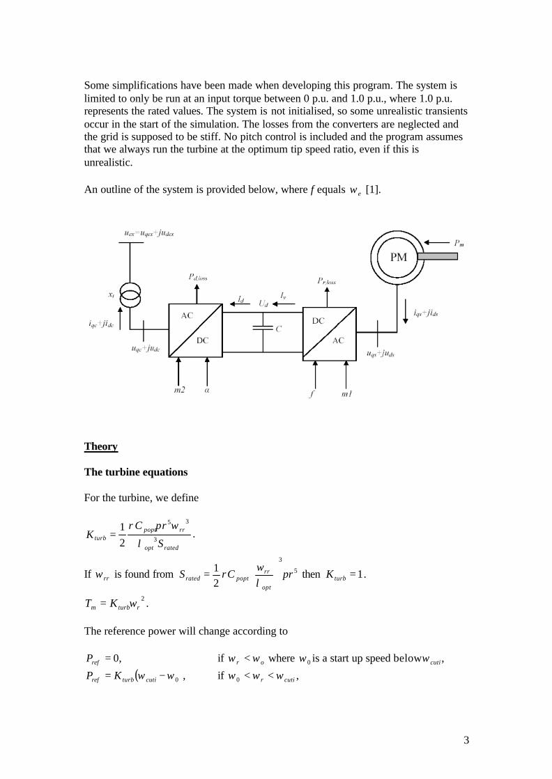
Some simplifications have been made when developing this program. The system is limited to only be run at an input torque between 0 p.u. and 1.0 p.u., where 1.0 p.u. represents the rated values. The system is not initialised, so some unrealistic transients occur in the start of the simulation. The losses from the converters are neglected and the grid is supposed to be stiff. No pitch control is included and the program assumes that we always run the turbine at the optimum tip speed ratio, even if this is unrealistic. An outline of the system is provided below, where f equals eω [1].

Theory The turbine equations For the turbine, we define

ratedopt

rrpoptturb

S

rCK 3

35

21

λ

ωπρ= .

If rrω is found from 5

3

21 rCS

opt

rrpoptrated π

λω

ρ

= then 1=turbK .

2rturbm KT ω= .

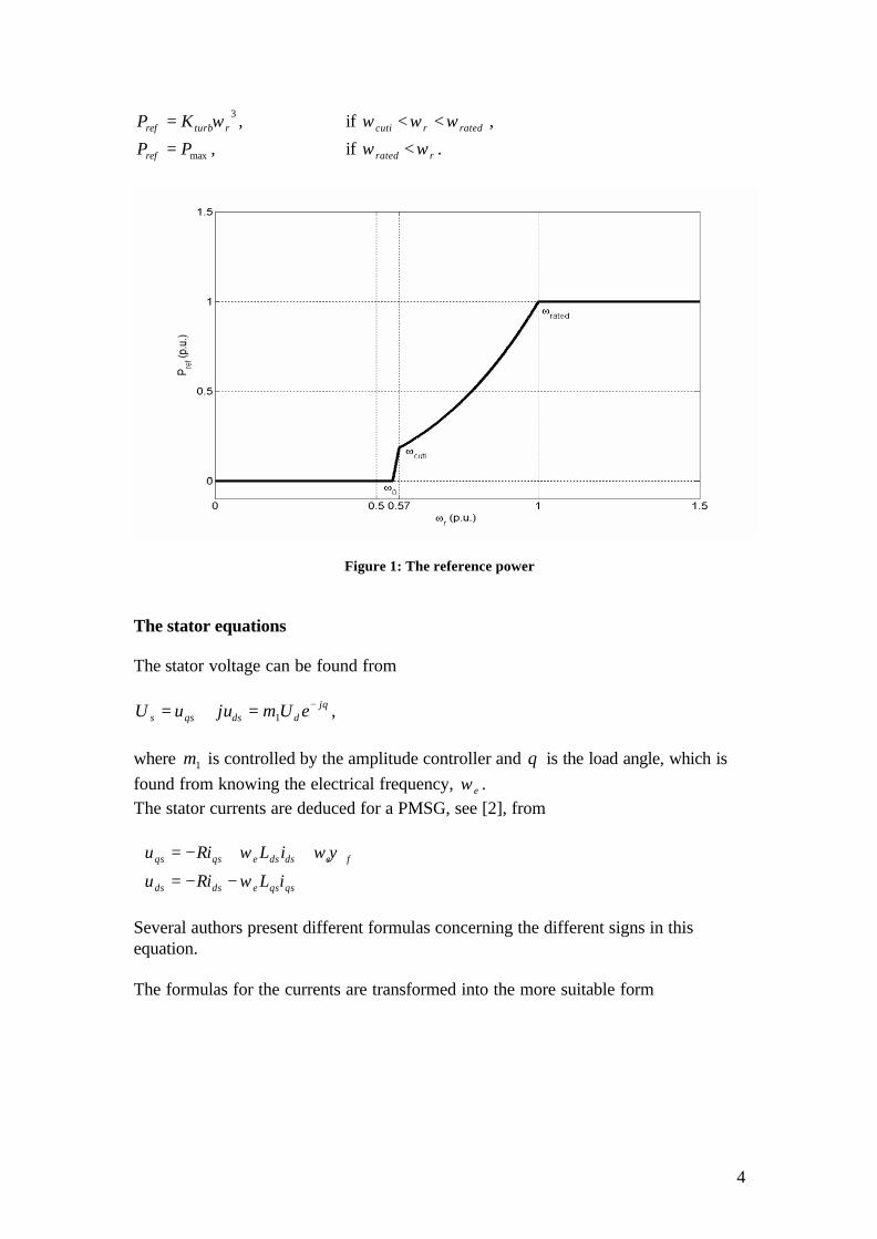
The reference power will change according to

,0=refP if or ωω < where 0ω is a start up speed below cutiω ,

( ),0ωω −= cutiturbref KP if cutir ωωω <<0 ,

4

,3rturbref KP ω= if ratedrcuti ωωω << ,

,maxPPref = if rrated ωω < .

Figure 1: The reference power The stator equations The stator voltage can be found from

θjddsqss eUmjuuU −=+= 1 ,

where 1m is controlled by the amplitude controller and θ is the load angle, which is found from knowing the electrical frequency, eω . The stator currents are deduced for a PMSG, see [2], from

−−=

++−=

qsqsedsds

fedsdseqsqs

iLRiu

iLRiu

ω

ψωω

Several authors present different formulas concerning the different signs in this equation. The formulas for the currents are transformed into the more suitable form

5

+

−+−=

+

+−−=

dsqse

fqseqsqsedsds

dsqse

fedsdseqsqs

LLR

LuLRui

LLR

RuLRui

22

2

22

ω

ψωω

ω

ψωω

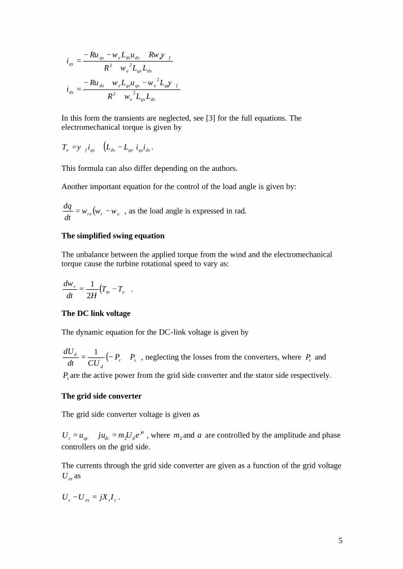
In this form the transients are neglected, see [3] for the full equations. The electromechanical torque is given by

( ) dsqsqsdsqsfe iiLLiT −+=ψ . This formula can also differ depending on the authors. Another important equation for the control of the load angle is given by:

( )erredtd

ωωωθ

−= , as the load angle is expressed in rad.

The simplified swing equation The unbalance between the applied torque from the wind and the electromechanical torque cause the turbine rotational speed to vary as:

( )emr TT

Hdtd

−=21ω

.

The DC link voltage The dynamic equation for the DC-link voltage is given by

( )scd

d PPCUdt

dU+−=

1, neglecting the losses from the converters, where cP and

sP are the active power from the grid side converter and the stator side respectively. The grid side converter The grid side converter voltage is given as

αjddcqcc eUmjuuU 2=+= , where 2m and α are controlled by the amplitude and phase

controllers on the grid side. The currents through the grid side converter are given as a function of the grid voltage

exU as

ctexc IjXUU =− .

6

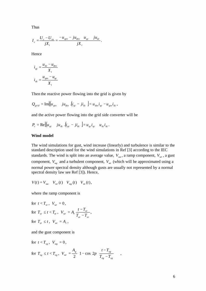
Thus

t

dcqcdexqex

t

excc jX

juujuujX

UUI

++−−=

−= .

Hence

−=

−=

t

qcqexdc

t

dexdcqc

X

uui

Xuu

i

Then the reactive power flowing into the grid is given by

( )( )[ ] dcqexqcdexdcqcdexqexgrid iuiujiijuuQ −=−+= .Im , and the active power flowing into the grid side converter will be

( ) ( )[ ] dcdcqcqcdcqcdcqcc iuiujiijuuP +=−+= .Re . Wind model The wind simulations for gust, wind increase (linearly) and turbulence is similar to the standard description used for the wind simulations in Ref [3] according to the IEC standards. The wind is split into an average value, waV , a ramp component, wrV , a gust component, wgV and a turbulent component, wtV (which will be approximated using a normal power spectral density although gusts are usually not represented by a normal spectral density law see Ref [3]). Hence,

)()()()( tVtVtVVtV wtwgwrwa +++= , where the ramp component is for srTt < , 0=wrV ,

for ersr TtT <≤ , srer

srrwr TT

TtAV

−−

= ,

for tTer ≤ , rwr AV = , and the gust component is for sgTt < , 0=wgV ,

for egsg TtT <≤ ,

−

−−=

sgeg

sggwr TT

TtAV π2cos1

2,

7

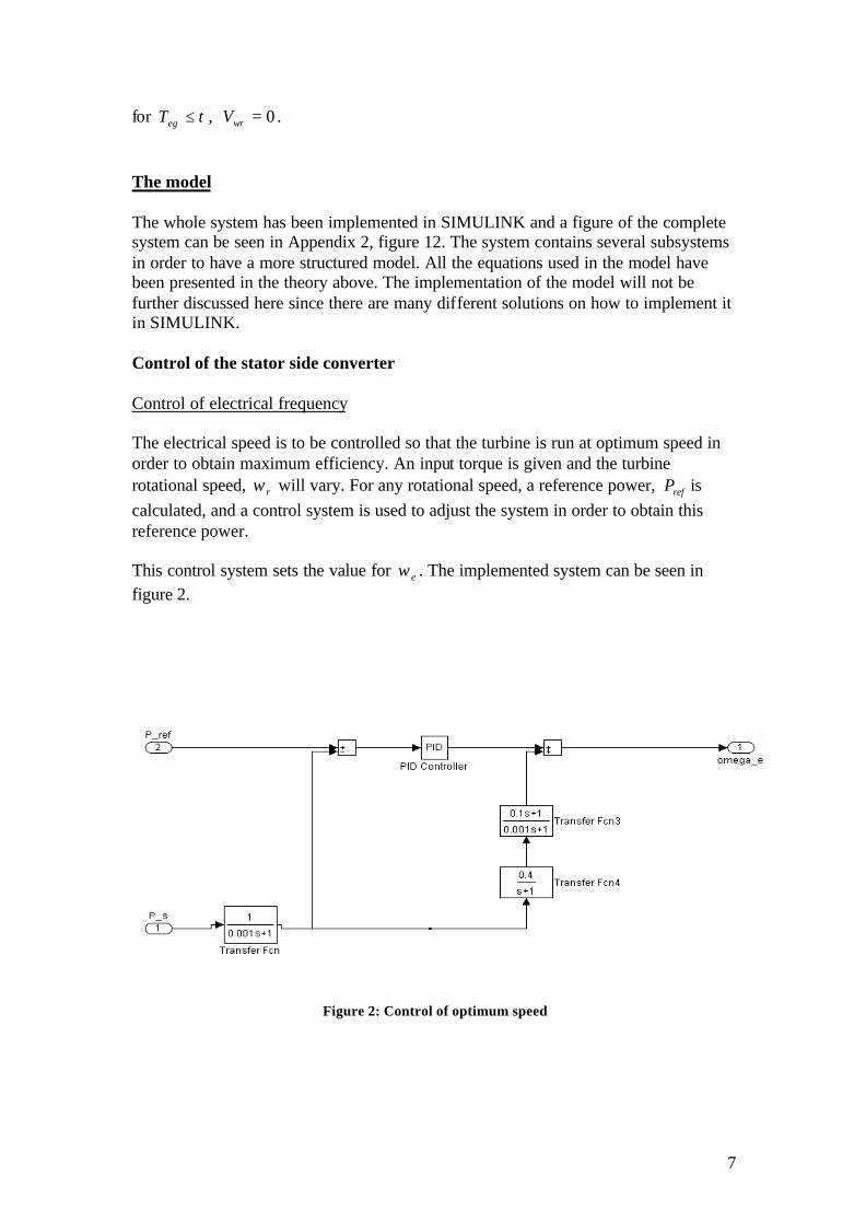
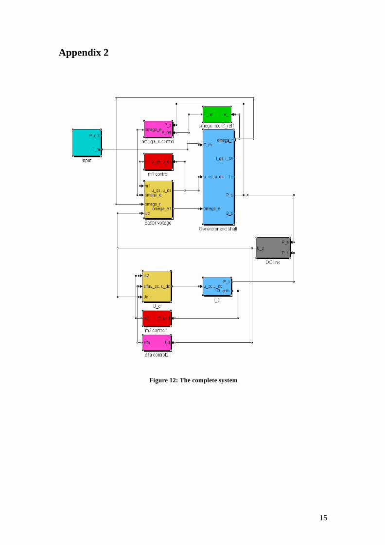
for tTeg ≤ , 0=wrV . The model The whole system has been implemented in SIMULINK and a figure of the complete system can be seen in Appendix 2, figure 12. The system contains several subsystems in order to have a more structured model. All the equations used in the model have been presented in the theory above. The implementation of the model will not be further discussed here since there are many different solutions on how to implement it in SIMULINK. Control of the stator side converter Control of electrical frequency The electrical speed is to be controlled so that the turbine is run at optimum speed in order to obtain maximum efficiency. An input torque is given and the turbine rotational speed, rω will vary. For any rotational speed, a reference power, refP is calculated, and a control system is used to adjust the system in order to obtain this reference power.

This control system sets the value for eω . The implemented system can be seen in figure 2.

Figure 2: Control of optimum speed

8

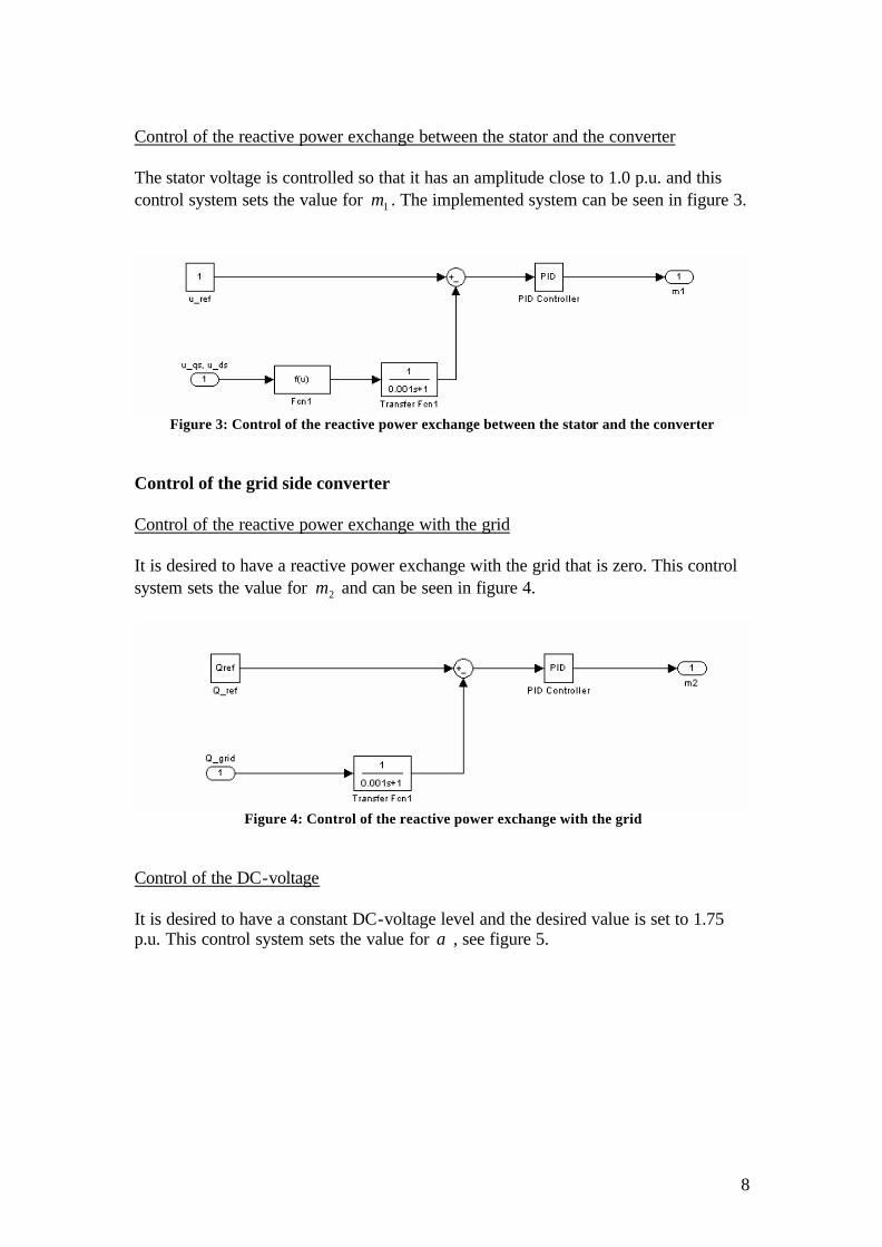
Control of the reactive power exchange between the stator and the converter The stator voltage is controlled so that it has an amplitude close to 1.0 p.u. and this control system sets the value for 1m . The implemented system can be seen in figure 3.

Figure 3: Control of the reactive power exchange between the stator and the converter

Control of the grid side converter Control of the reactive power exchange with the grid It is desired to have a reactive power exchange with the grid that is zero. This control system sets the value for 2m and can be seen in figure 4.

Figure 4: Control of the reactive power exchange with the grid

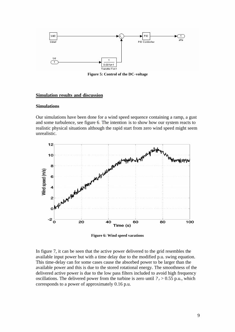
Control of the DC-voltage It is desired to have a constant DC-voltage level and the desired value is set to 1.75 p.u. This control system sets the value for α , see figure 5.

9

Figure 5: Control of the DC-voltage

Simulation results and discussion Simulations Our simulations have been done for a wind speed sequence containing a ramp, a gust and some turbulence, see figure 6. The intention is to show how our system reacts to realistic physical situations although the rapid start from zero wind speed might seem unrealistic.

Figure 6: Wind speed varations

In figure 7, it can be seen that the active power delivered to the grid resembles the available input power but with a time delay due to the modified p.u. swing equation. This time-delay can for some cases cause the absorbed power to be larger than the available power and this is due to the stored rotational energy. The smoothness of the delivered active power is due to the low pass filters included to avoid high frequency oscillations. The delivered power from the turbine is zero until ? r > 0.55 p.u., which corresponds to a power of approximately 0.16 p.u.

10

Figure 7: Power variations. The smooth line is Pc and the other line available power

The DC-link voltage is to be kept at 1.75 p.u. which is the case in figure 8. In addition we do not want any reactive power delivered to the grid and this is accomplished as can be seen in figure 9.

Figure 8: DC-voltage

11

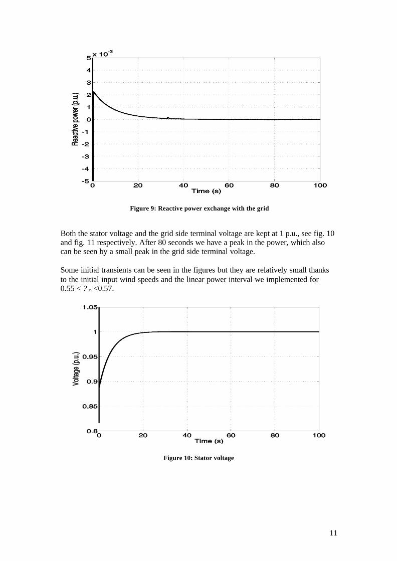
Figure 9: Reactive power exchange with the grid

Both the stator voltage and the grid side terminal voltage are kept at 1 p.u., see fig. 10 and fig. 11 respectively. After 80 seconds we have a peak in the power, which also can be seen by a small peak in the grid side terminal voltage. Some initial transients can be seen in the figures but they are relatively small thanks to the initial input wind speeds and the linear power interval we implemented for 0.55 < ? r <0.57.

Figure 10: Stator voltage

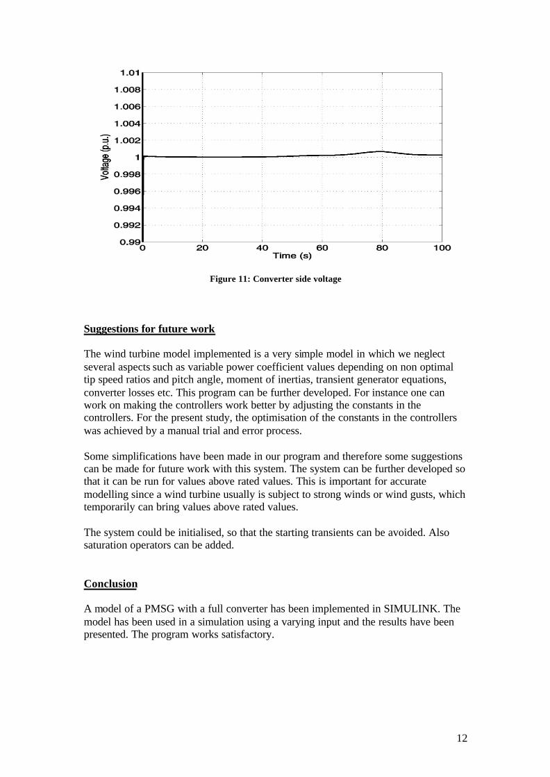
12

Figure 11: Converter side voltage

Suggestions for future work The wind turbine model implemented is a very simple model in which we neglect several aspects such as variable power coefficient values depending on non optimal tip speed ratios and pitch angle, moment of inertias, transient generator equations, converter losses etc. This program can be further developed. For instance one can work on making the controllers work better by adjusting the constants in the controllers. For the present study, the optimisation of the constants in the controllers was achieved by a manual trial and error process. Some simplifications have been made in our program and therefore some suggestions can be made for future work with this system. The system can be further developed so that it can be run for values above rated values. This is important for accurate modelling since a wind turbine usually is subject to strong winds or wind gusts, which temporarily can bring values above rated values. The system could be initialised, so that the starting transients can be avoided. Also saturation operators can be added. Conclusion A model of a PMSG with a full converter has been implemented in SIMULINK. The model has been used in a simulation using a varying input and the results have been presented. The program works satisfactory.

13

References [1] Ian Norheim, Dynamic modelling of turbines(2), Regulation and control strategies(1), lecture notes, Nordic PhD course on wind power, Smöla, Norway, 050607 [2] P.Kundur, Power System Stability and Control, McGraw-Hill, Inc. 1994. [3] T. Ackermann, Wind Power in Power Systems, Wiley, 2005.

14

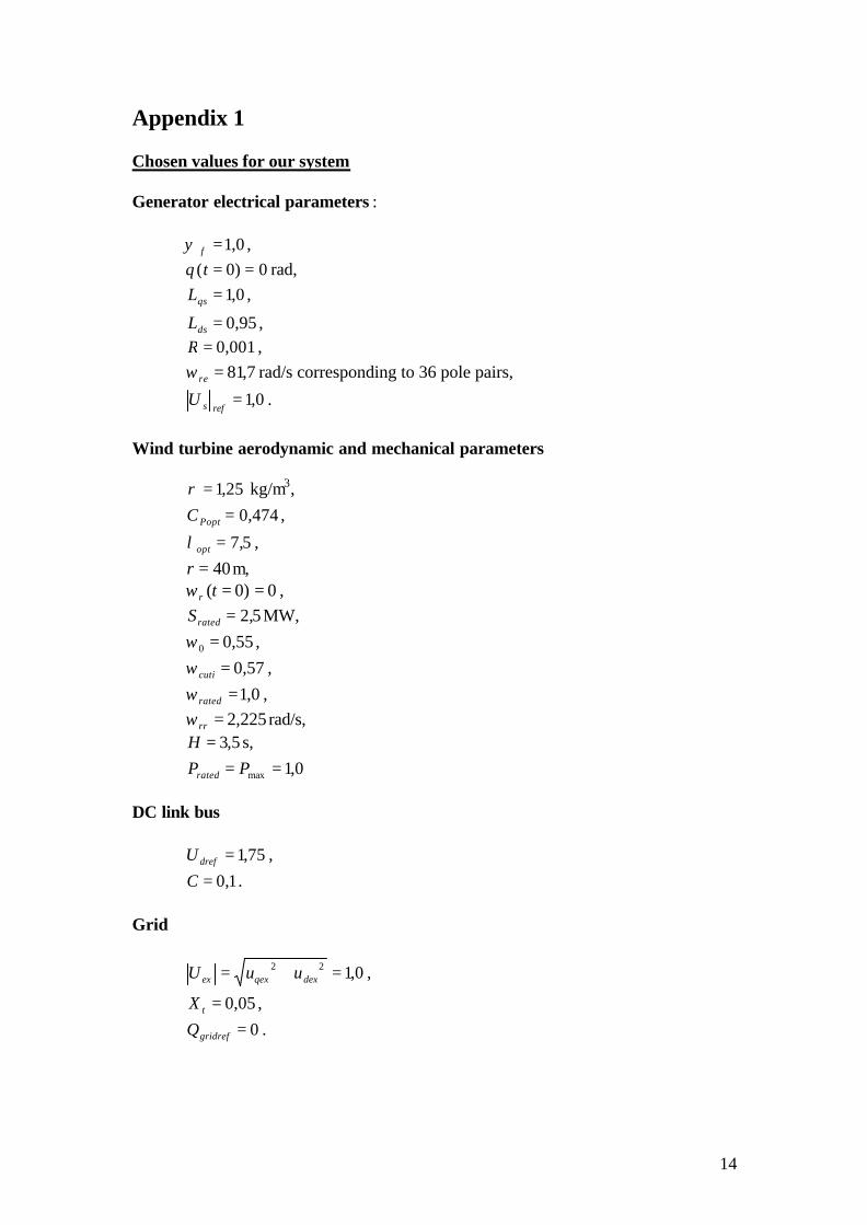
Appendix 1 Chosen values for our system Generator electrical parameters : 0,1=fψ , 0)0( ==tθ rad, 0,1=qsL ,

95,0=dsL , 001,0=R , 7,81=reω rad/s corresponding to 36 pole pairs,

0,1=refsU .

Wind turbine aerodynamic and mechanical parameters 25,1=ρ kg/m3, 474,0=PoptC ,

5,7=optλ , 40=r m, 0)0( ==trω , 5,2=ratedS MW, 55,00 =ω , 57,0=cutiω , 0,1=ratedω , 225,2=rrω rad/s, 5,3=H s, 0,1max == PPrated DC link bus 75,1=drefU , 1,0=C . Grid

0,122 =+= dexqexex uuU ,

05,0=tX , 0=gridrefQ .

15

Appendix 2

Figure 12: The complete system