Simulation & Analysis of the Helicopter Transmission System · Abstract This report analyzes the main shafts of the helicopter transmission box. The corresponding behavior of the

Simulation & Analysis of the Helicopter Transmission

System

الطائرة العموديةنظام نقل الحركة الخاص ب حليلتمحاكاة و

by

ABDALLAH LASFER

Dissertation submitted in fulfilment

of the requirements for the degree of

MSc SYSTEMS ENGINEERING

at

The British University in Dubai

January 2019

DECLARATION

I warrant that the content of this research is the direct result of my own work and that any use

made in it of published or unpublished copyright material falls within the limits permitted by

international copyright conventions. I understand that a copy of my research will be deposited

in the University Library for permanent retention. I hereby agree that the material mentioned

above for which I am author and copyright holder may be copied and distributed by The British

University in Dubai for the purposes of research, private study or education and that The British

University in Dubai may recover from purchasers the costs incurred in such copying and

distribution, where appropriate. I understand that The British University in Dubai may make a

digital copy available in the institutional repository. I understand that I may apply to the

University to retain the right to withhold or to restrict access to my thesis for a period which

shall not normally exceed four calendar years from the congregation at which the degree is

conferred, the length of the period to be specified in the application, together with the precise

reasons for making that application.

_______________________

Signature of the student

COPYRIGHT AND INFORMATION TO USERS

The author whose copyright is declared on the title page of the work has granted to the British

University in Dubai the right to lend his/her research work to users of its library and to make

partial or single copies for educational and research use. The author has also granted permission

to the University to keep or make a digital copy for similar use and for the purpose of

preservation of the work digitally. Multiple copying of this work for scholarly purposes may be

granted by either the author, the Registrar or the Dean only. Copying for financial gain shall

only be allowed with the author’s express permission. Any use of this work in whole or in part

shall respect the moral rights of the author to be acknowledged and to reflect in good faith and

without detriment the meaning of the content, and the original authorship.

Abstract

This report analyzes the main shafts of the helicopter transmission box. The

corresponding behavior of the shafts, gears, and blades are monitored and studied.

Three different methods were used to analyze the set of systems describing the

behavior of the shafts. The first method is the lumped model analysis, which

considers each element of the shaft to be discrete. The second method is the finite

element method, which separates the shaft itself into smaller elements. The last

method is the hybrid model, where the gears are taken as discrete elements, while

the shaft characteristics are continuous functions of the shafts’ length. The speed at

each end of each shaft is recorded and studied, as well as, the shafts threshold to the

shear stress applied. The model results are compared for accuracy, precision and

difficulty. Results conclude of simplicity of the lumped model but also

impracticality. While the finite elements model is difficult to produce as it requires

tedious solving of high order polynomials. The hybrid model is the most accurate in

terms of shaft properties however; it faces difficulty in determining the critical

speeds for mechanical failure.

ملخص

صاا لللذا ديسللللر رلللل لار سألايحللللذا لللقرار األعيلللعارئيسللللصار ع إرلللإاا للللبلر.ايتملللاقار ولإاللل اع ايلللا ا عر لللاار ترملللا

ص ارر شلللتعرت االلل ارملللاطلر اخلللة اتلللع.ا طالتلللاا احلإلللذا صس يلللاا للل ار لللب ار اللل االللل املللل لارئيسللللارر الللعر

ااحلإللللذار بسللل طوار سألطللل ياتارر لللقصايما للللعاعلللذايبللللعا للل ايبا للللعايسللل ار سب للل ا بتلللللةاار طعيأللللاارئر للل ا للل ا

األلللاارئةإلللعصر طعيأللللاار يا إلللاا للل اتعيأللللاار مبا لللعار سحللللر صاتار اللل ااتللللذار مسللل ا ترللل اي للل ايبا لللعا للل ع ارر طعي

لاتااماسللل للل ار بسللل طوار وصلللإ اتاخإلللتايلللا ا ةلللقار الللعر اعمبا لللعا بتلللللااتااللل اخلللإ اااللل اةللللا ار مسللل ا لللتا

وللا ار أللل ايللل اتلل قار مسلل ايللا اارللصإذار ترمللاار رللعياايبلللاعللذا وايللاا اللذايسلل اتارعللق ايا للاار مسلل اي لل اي

اا سألطللل يا ولللر سط أللللا االللا ا ألات لللاا الللا ار بسللل طوا للل اخإلللتار ل لللاارر للللم ا االطللل ار بالللا ا للل ا اخإلللاار بسللل طوار

ا لللا اا رلللإطاار اللل الإلللعايسلإلللا االلل اخلللإ ايللللم اخلللذا ملللا تا سللل طوا ا ار مبا لللعار سحللللر صائ ولللااااطلللل اخلللةا

لللاار رللعياار حعار بسلل طوار وصللإ ا للل ارئعيللعا لللاا لل اخإللتاةللللا ات للبار للل اط لل ا اا ر لل ا لللم ااالل ااحليلللل

لتشذار سإاا إا

Acknowledgment

I would like to thank my supervisor, Dr Alaa Ameer for his continuous guidance and

for providing assistance and advice when needed.

I also would like to show gratitude towards Professor Robert Whalley (deceased) for

his teachings and help throughout the whole program.

I am grateful towards my family, friends and colleagues for providing the physical

and mental encouragement to pursue this degree.

I

Table of Contents

List of Illustrations ....................................................................................................................................

List of Abbreviations .................................................................................................................................

Chapter I: Introduction ............................................................................................................................ 1

1.1 Control Systems Engineering Background ................................................................................... 1

1.2 Mathematical Modelling ............................................................................................................... 4

1.2.1 Lumped Parameter Method .................................................................................................... 4

1.2.2 Finite Element Method ........................................................................................................... 5

1.2.3 Hybrid (Distributed-Lumped) Method ................................................................................... 5

1.3 Problem Statement ........................................................................................................................ 6

1.4 Aims and Objectives ..................................................................................................................... 7

1.5 Organization of the Dissertation ................................................................................................... 7

Chapter II: Literature Review ................................................................................................................. 9

2.1 History of the Helicopter Aircraft ................................................................................................. 9

2.2 Helicopter Flight Principle ............................................................................................................ 9

2.3 Helicopter Transmission Line Components ................................................................................ 10

2.3.1 Gas Turbine & Turbo shaft .................................................................................................. 11

2.3.2 Clutch ................................................................................................................................... 14

2.3.3 Gears .................................................................................................................................... 16

2.4 Lumped Parameter Method ......................................................................................................... 17

2.5 Finite Element Method ................................................................................................................ 18

2.6 Impedance Analogy..................................................................................................................... 19

2.7 Hybrid (Distributed-Lumped) Method ........................................................................................ 20

Chapter III: Mathematical Modeling ..................................................................................................... 22

3.1 Helicopter Transmission System Model ..................................................................................... 22

3.2 Lumped Parameter Model ........................................................................................................... 23

3.3 Finite Elements Model ................................................................................................................ 35

3.4 Hybrid (Distributed-Lumped) Model .......................................................................................... 52

3.5 Defining of Parameter Values & Equations for each Modeling Method .................................... 66

II

3.5.1 Lumped Parameter Model Equations ................................................................................... 66

3.5.2 Finite Element Model Equations .......................................................................................... 74

3.5.3 Hybrid (Distributed-Lumped) Model Equations .................................................................. 79

Chapter IV: Simulation, Results & Discussion of Results .................................................................... 82

4.1 Lumped Parameter Model Simulation ........................................................................................ 82

4.2 Lumped Parameter Model Results .............................................................................................. 85

4.3 Lumped Parameter Model Analysis ............................................................................................ 93

4.4 Finite Element Model Simulation ............................................................................................... 99

4.5 Finite Element Model Results ................................................................................................... 102

4.6 Finite Element Model Analysis ................................................................................................. 112

4.7 Hybrid (Distributed-Lumped) Model Simulation ..................................................................... 117

4.8 Hybrid (Distributed-Lumped) Model Results ........................................................................... 121

4.9 Hybrid (Distributed-Lumped) Model Analysis ......................................................................... 127

Chapter V: Conclusions & Recommendations .................................................................................... 131

References ........................................................................................................................................... 133

Appendix I ........................................................................................................................................... 136

Appendix II ......................................................................................................................................... 150

8.1 Definition of Concepts .............................................................................................................. 150

8.1.1 Torque& Torsion ................................................................................................................ 150

8.1.2 Shear Stress ........................................................................................................................ 151

8.1.3 Angular Displacement, Velocity, Acceleration .................................................................. 151

8.1.4 Inertia & Moment of inertia ............................................................................................... 152

8.1.5 Power .................................................................................................................................. 153

8.1.6 Density ............................................................................................................................... 153

8.2 Differential Equations ............................................................................................................... 153

III

List of Illustrations

Figure 1: Overview of the Components of the Helicopter Transmission System (FAA Safety Team,

Accessed 6 Jan 2019) ............................................................................................................................ 11

Figure 2: Compressor Flow Characteristics (Fundamentals of Gas Turbine Engines, Accessed 14 Oct

2018) ..................................................................................................................................................... 13

Figure 3: Turbine Flow Characteristics (Fundamentals of Gas Turbine Engines, Accessed 14 Oct

2018) ..................................................................................................................................................... 13

Figure 4: Side View of the Components of a Turbo Shaft (Turbo Shaft Operation, Accessed on Jan 3

2019) ..................................................................................................................................................... 14

Figure 5: The Belt Drive Clutch (Padfield, 2013) ................................................................................. 15

Figure 6: Illustration of a Gear Train (Integrated Publishing, Accessed on Dec 21 2018) ................... 17

Figure 7: Schematic Model of the Helicopter Transmission System .................................................... 23

Figure 8: Main Rotor Shaft (MRS) ....................................................................................................... 24

Figure 9: Main Rotor Shaft (MRS): Labeled ........................................................................................ 25

Figure 10: Block Diagram of Lumped Model on Main Rotor Shaft ..................................................... 31

Figure 11: Block Diagram of Main Shaft .............................................................................................. 34

Figure 12: Finite Element Model on Main Rotor Shaft ........................................................................ 35

Figure 13: Block Diagram of the Finite Element Model on Main Rotor Shaft ..................................... 44

Figure 14: The Block Diagram of the Finite Element Model on Main Shaft ........................................ 51

Figure 15: Hybrid Model Main Rotor Shaft Labeled ............................................................................ 52

Figure 16: Transmission Line Representation (Whalley, Ebrahimi, Jamil, 2005) ................................ 53

Figure 17: Block Diagram of the Hybrid Model on Main Rotor Shaft ................................................. 62

Figure 18: Block Diagram of the Hybrid Model on the Main Shaft ..................................................... 65

Figure 19: Representation of SIMULINK Model of Main Rotor Shaft ................................................ 82

Figure 20: Representation of SIMULINK Model Main Shaft .............................................................. 84

Figure 21: Load End (Angular Speed 1) of Lumped Model ................................................................. 85

Figure 22: Drive End (Angular Speed 2) of Lumped Model ................................................................ 86

Figure 23: Load End (Angular Speed 1) Bode Plot for Lumped Model ............................................... 86

Figure 24: Load End (Angular Speed 2) Bode Plot for Lumped Model ............................................... 87

Figure 25: Shear Stress of Main Rotor Shaft for Lumped Model ......................................................... 88

Figure 26: Tail Rotor Speed for Lumped Model ................................................................................... 89

Figure 27: Drive End (Angular Speed 4) of Main Shaft for Lumped Model ........................................ 89

Figure 28: Blade Angular Speed of Main Shaft for Lumped Model ..................................................... 90

Figure 29: Drive End (Angular Speed 4) of Main Shaft Bode plot for Lumped Model ....................... 91

Figure 30: Blade Angular Speed of Main Shaft Bode Plot for Lumped Model .................................... 92

Figure 31: Shear Stress of Main Shaft for Lumped Model ................................................................... 93

Figure 32: Representation of SIMULINK Model of Finite Elements on Main Rotor Shaft ............... 100

Figure 33: Representation of SIMULINK Model of Main Shaft for the Finite Elements .................. 101

Figure 34: Load End (Angular Speed 1) of Finite Model ................................................................... 102

IV

Figure 35: Drive End (Angular Speed 2) of Finite Element Model .................................................... 103

Figure 36: Load End (Angular Speed 1) Bode Plot for Finite Element Model ................................... 104

Figure 37: Load End (Angular Speed 2) Bode Plot for Finite Element Model ................................... 105

Figure 38: Shear Stress of Main Rotor Shaft for Finite Element Model ............................................. 106

Figure 39: Tail Rotor Speed for Finite Element Model ...................................................................... 107

Figure 40: Drive End (Angular Speed 4) of Main Shaft for Finite Element Model............................ 108

Figure 41: Blade Angular Speed of Main Shaft for Finite Element Model ........................................ 109

Figure 42: Drive End (Angular Speed 4) of Main Shaft Bode plot for Finite Element Model ........... 110

Figure 43: Blade Angular Speed of Main Shaft Bode Plot for Finite Element Model ........................ 111

Figure 44: Shear Stress of Main Shaft for Finite Element Model ....................................................... 112

Figure 45: Representation of SIMULINK Model on Main Rotor Shaft for Hybrid Model ................ 118

Figure 46: Representation of SIMULINK Model on Main Shaft for Hybrid Model .......................... 120

Figure 47: Load End (Angular Speed 1) of Hybrid Model ................................................................. 121

Figure 48: Drive End (Angular Speed 2) of Hybrid Model ................................................................ 122

Figure 49: Shear Stress Main Rotor Shaft Hybrid Model ................................................................... 123

Figure 50: Tail Rotor Speed Hybrid Model ........................................................................................ 124

Figure 51: Drive End (Angular Speed 4) of Main Shaft for Hybrid Model ........................................ 125

Figure 52: Blade Angular Speed of Main Shaft for Hybrid Model ..................................................... 126

Figure 53: Shear Stress Main Shaft Hybrid Model ............................................................................. 127

Figure 54: Shear stress distribution across Solid and Hollow Shafts .................................................. 151

Figure 55: Equations of moment and polar moment of inertia for different shapes of rigid bodies ... 153

V

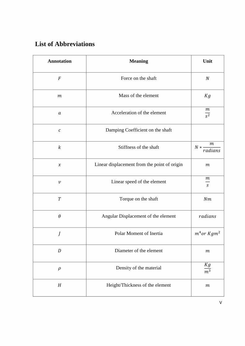
List of Abbreviations

Annotation Meaning Unit

𝐹 Force on the shaft 𝑁

𝑚 Mass of the element 𝐾𝑔

𝑎 Acceleration of the element 𝑚

𝑠2

𝑐 Damping Coefficient on the shaft

𝑘 Stiffness of the shaft 𝑁 ∗𝑚

𝑟𝑎𝑑𝑖𝑎𝑛𝑠

𝑥 Linear displacement from the point of origin 𝑚

𝑣 Linear speed of the element 𝑚

𝑠

𝑇 Torque on the shaft 𝑁𝑚

𝜃 Angular Displacement of the element 𝑟𝑎𝑑𝑖𝑎𝑛𝑠

𝐽 Polar Moment of Inertia 𝑚4𝑜𝑟 𝐾𝑔𝑚2

𝐷 Diameter of the element 𝑚

𝜌 Density of the material 𝐾𝑔

𝑚3

𝐻 Height/Thickness of the element 𝑚

VI

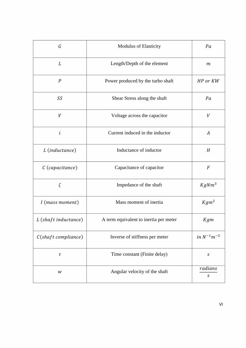
𝐺 Modulus of Elasticity 𝑃𝑎

𝐿 Length/Depth of the element 𝑚

𝑃 Power produced by the turbo shaft 𝐻𝑃 𝑜𝑟 𝐾𝑊

𝑆𝑆 Shear Stress along the shaft 𝑃𝑎

𝑉 Voltage across the capacitor 𝑉

𝑖 Current induced in the inductor 𝐴

𝐿 (𝑖𝑛𝑑𝑢𝑐𝑡𝑎𝑛𝑐𝑒) Inductance of inductor 𝐻

𝐶 (𝑐𝑎𝑝𝑎𝑐𝑖𝑡𝑎𝑛𝑐𝑒) Capacitance of capacitor 𝐹

𝜁 Impedance of the shaft 𝐾𝑔𝑁𝑚3

𝐼 (𝑚𝑎𝑠𝑠 𝑚𝑜𝑚𝑒𝑛𝑡) Mass moment of inertia 𝐾𝑔𝑚2

𝐿 (𝑠ℎ𝑎𝑓𝑡 𝑖𝑛𝑑𝑢𝑐𝑡𝑎𝑛𝑐𝑒) A term equivalent to inertia per meter 𝐾𝑔𝑚

𝐶(𝑠ℎ𝑎𝑓𝑡 𝑐𝑜𝑚𝑝𝑙𝑖𝑎𝑛𝑐𝑒) Inverse of stiffness per meter 𝑖𝑛 𝑁−1𝑚−2

𝜏 Time constant (Finite delay) 𝑠

𝑤 Angular velocity of the shaft 𝑟𝑎𝑑𝑖𝑎𝑛𝑠

𝑠

1

Chapter I: Introduction

1.1 Control Systems Engineering Background

The discipline of control system engineering is the study that uses the control

theory to manipulate different and a wide range of systems based and derived

from their mathematical roots. Sensors are used to measure the output of the

modelled and analysed system. The signals from the output measurement are

used as a method of corrective feedback to correct the input signal and reach the

desired outcome of the system. Control systems engineering is a very large field

with many sub specialties originating from different disciplines of engineering,

such as mechanical, electrical, chemical, and computer engineering. The very

first work in automatic control was the speed control of a rotor powered by a

steam engine in the eighteenth century (Ogata, 1997). In the early 1900s

engineers such as Harry Nyquist started developing different ways in terms of

finding stability of closed loop systems. During the mid-1900s, the frequency

response and root locus methods were fully developed as a basis and core of

classical control theory.

The analysis of any controlled system is divided in two categories.

Modelling and Simulation

Control Theory

The study of modelling in control systems engineering involves going back to the

roots of practical physics, and deriving the mathematical equations that describe the

2

analysed dynamic system. Current modelling techniques involves the use of

frequency response to turn ordinary and partial differential equations into

polynomials that are easier to solve. The model of the dynamic controlled system

covers the governing equations as well as some assumptions and constraints. This is

an integral part of the determining the solution of the equations. As mathematics

dictate, the solutions of differential equations are generated from a general format.

This general format is made smaller and more specific to one specific case by the

use of initial boundary conditions (A.D.Polyanin, 2003). These boundary conditions

are specific to the problem at hand and determined by the engineer.

With the help of new software and the mechanical to electrical analogies, it is

possible to simulate the dynamic system. Simulation is done after modelling; it

helps in understanding the behaviour of the designated system without the

requirement of building the prototype (up to an extent). With simulation, it is

possible to duplicate and imitate the initial signals sent to the system in order to

observe the behavioural response of the output.

Different modelling techniques exist, with different accuracies and difficulties; it

is the job of the engineer to analyse and optimise the best solution according to

the desired and required performance. For the case of drive line systems, the

models are linear, dynamic, discrete and continuous depending on the method

used. Further details will be explained in the following chapter.

The application of the control theory is related to the feedback control system.

The governing equations of the dynamic system can be represented in a block

3

model, this is also known as the open loop response. In order to close the loop, a

controller must be added; however, the design of the controller depends on the

system dynamics. In case of a single input command, and a single output from

the actuator, a more classical approach is used. A feedback is added that takes the

measured output signal and feeds it to the controller (Ogata, 1997). The

controller compares the output with the input signal it receives and corrects the

input. This is done continuously while the system is running; decreasing the

margin of error every time the signal passes through the loop until a steady state

is achieved. The main function of the controller is to be able to keep this steady

state output in case of any disturbances on the system. An example of a single

input-output controller is the PID, or the Proportional Integral Differential

controller, which regulates the response output of the system by increasing the

amplitude (of the signal), reducing the steady state error, regulating the overshoot

and the settling time (Sontag, 1998). In case of multiple input-output systems, a

more modern approach is used. The mathematical modelling for these type of

systems usually need a state space representation, and is solved in a matrix.

Designing a controller for these types of systems usually involves a lot more

complex methods with the help of software to produce more accurate results, as

the math can get very tedious. This becomes much more complicated in higher

order systems (3 or more input to outputs).

This is the case for all stable open-loop systems, in case of unstable systems a

test of controllability must be done first to determine if closing the loop can

4

control the Eigenvalues (roots of the equations) of the system (and to what

extent).

This dissertation will not cover the control theory, but only the modelling and

simulation of the main transmission of a helicopter vehicle.

1.2 Mathematical Modelling

The modeling of helicopter transmission is used to derive the basic mathematical

equations that describe the rotor shaft dynamic system.

Three different modeling techniques are used to study the behavior of the

helicopter transmission:

1- The Lumped Parameter Method

2- The Finite Element Method

3- The Hybrid (Distributed-Lumped) Method

The three models are used to describe the dynamic system in terms of differential

and partial differential equations within certain assumptions in order to analyze

the dynamic shear stresses and angular speeds of the shafts.

1.2.1 Lumped Parameter Method

The lumped parameter method is a method that describes the distributed system

in a topology. This topology is made of discrete elements that explain how the

system behaves under certain conditions and constraints. However, the lumped

model usually consists of an element having one important physical property

(Doebelin, E.O, 1998.). That physical property of concern will be a function of

5

one variable. What this signifies is that it reduces the set of equations that

describe the system into a number of ordinary differential equations with finite

number of parameters. This method is mainly but not entirely used in electrical,

thermal and mechanical systems.

1.2.2 Finite Element Method

The finite element method is a type of numerical methods to solve problems in

physics and engineering by approximating solutions of complex differential

equations. Differential equations are solved usually by having initial boundary

conditions to be set, so that the general solution is extracted. Some partial

differential equations are unsolvable unless a boundary condition is set, to extract

a specific solution for a specific problem. The finite element method divides a

problem into smaller parts named after the method. These equations are

transformed into algebraic polynomials, and then combined to form the system of

equations that model the problem (K.J.Bathe, 1976). The finite element method

is used in many disciplines of engineering and physics usually involving

dynamics of elements such as heat transfer, fluid flow dynamics, structural

analysis, and rotor systems.

1.2.3 Hybrid (Distributed-Lumped) Method

The model is derived based on the electrical transmission line using two linear

differential equations. These equations are called the telegrapher equations; they

were developed by Oliver Heaviside sometime in the late 19th century. The

equations are described by voltage and current those vary with time and the

6

length of the transmission line. These equations can be applied to all types of

transmission lines regardless of frequency. The transmission line model consists

of a resistor and an inductor in series, followed by another resistor and a

capacitor connected to it in parallel (Karakash, John,1950). The effect of the

inductance in the model is similar to that of the inertia in rigid bodies. The effect

of the capacitance is the same as of that of the spring, as it behaves as a restoring

force. The resistors exist as an energy dissipater, but in the lossless transmission

line model, they are equal to zero. All elements in the model are variables of

length. This is the base model used to derive the equations used in the hybrid

model analysis. This is because the hybrid model describes the shaft length as a

function of its inductance and compliance, similarly to the transmission line

model. However, lumped elements also exists in the model, such as the inertia of

the shafts/gears, length, diameter, and damping.

1.3 Problem Statement

The reason the helicopter transmission is studied, analysed and simulated is to

understand the difficulties in design in order to control and reduce the problems

that could occur due to torsional stresses in the shafts. The main purpose of this

dissertation is to apply the lumped, finite element, and transmission line

modelling techniques to the helicopter transmission system, and to compare the

accuracy and precision, difficulty, complexity, and the response of each model in

order to fully understand the behaviour of the system. The analysis will include

7

the speed of the shafts, as well as the shear stress. Bode diagrams will be used to

identify resonance speeds.

1.4 Aims and Objectives

At the end of the dissertation, the reader will be able to comprehend the

following:

Mathematical modelling of the helicopter transmission model using lumped,

finite element and hybrid model techniques.

Simulation of the helicopter transmission model on SIMULINK software.

Study and analyse the behaviour of the system from the response and bode

plots in terms of angular speed and dynamic torsional stress.

Comparing all modelling techniques in terms of response, complexity,

accuracy and feasibility to conclude the optimised way of analysis.

1.5 Organization of the Dissertation

The dissertation will consist of five different chapters:

Chapter one contains the introduction and background. This introduces the reader

mathematical modelling. Moreover, it presents the fundamental basics behind the

three methods that will be used.

Chapter two contains the literature review. This is the history of the helicopter,

how it was made, the flight principle, and the components that make the aircraft.

The three modelling techniques developed to simulate and analyse the helicopter

8

transmission is discussed as used by mathematicians, engineers, researchers and

scholars; showing what has been done (work) and their opinion (conclusions).

Chapter three covers the actual mathematical modelling and derivation. This

section covers the explanation of how the model is derived, as well as the

solution for the equations. The parameter definitions, values and calculations are

all completed in this chapter.

Chapter four shows the simulation, results, and the discussion of the three

models. This section describes the results in terms of the responses of the system.

The angular speed and shear stresses of each shaft is analysed. In addition, the

settling time, overshoot, magnitude, phase, and resonance speeds are recorded

and studied. Results are explained based on values reached.

Chapter five explains the conclusions reached. This is the author’s scientific

opinion based on the results obtained from the simulation. Each model’s results

are compared based on their qualities in terms of complexity, accuracy and

difficulty. A final conclusion is reached, and recommendations can be given if

needed.

9

Chapter II: Literature Review

2.1 History of the Helicopter Aircraft

The word helicopter comes from the greek words “helix” and “pteron” meaning

“spiral” and “wing”. The very first inventor (that was recorded in history) is said to

be the famous Leonardo da Vinci (Prime Industries, 2015). He was fascinated with

the idea of a flying machine with a helical screw which he designed in 1488.

However, due to lack of means he was never able to build it. This inspiration took

on into Sikorsky, the first man to build the base design of many modern helicopters.

The main struggle in creating the helicopter was the maneuvering of the main rotor

blades, which was solved by the mechanics of the swash plate. The swash plate is

able to move the rotor blades at different angles to allow sideway movements; the

main difference between a helicopter and an airplane. Another problem was the

design of the tail rotor blade, this was used to counter act the torque from the main

rotor blades. It was only until 1942 where Sikorsky was able to design the very first

successful helicopter.

2.2 Helicopter Flight Principle

The helicopter flight principle is based on the lift force produced from the main

rotor. When the fuel burns, the turbo shaft rotates the shaft, and power is

transmitted to the main rotor through the helicopter transmission. When the

rotor blades rotate, due to the shape of the blade, it creates a pressure difference

which causes a force upwards (Lift Force).

10

When the lift is more than the weight of the helicopter, it starts to move upwards

(Seddon and Newman, 2011). Navigation on the helicopter (movement to the

right/left or upwards/downwards) is done through changing the angle of attack.

This is the angle between the edge of the blade and the streamline of air hitting

the blade. The change in angle of attack decomposes the force vector into

different axes depending of direction of desire. This change is done using a

swashbuckler located at the hub connected below the rotor. When moving the

controls of the helicopter, the swashbuckle slips and twists accordingly to

change the angle of attack of the blades in order to manoeuvre around. Rotation

of the main rotor blades causes a problem that can be explained using Newton’s

third law of motion. For every action there is an equal and opposite reaction.

Because the main rotor blade rotates in one direction it will cause the body of

the helicopter to rotate as well. This is solved by installing the tail blade rotor.

The tail blade rotor’s main function is to counter act the force of rotation caused

by the main blade rotor (Padfield, 2013). The tail blade rotor produces a force in

a plane perpendicular to the main blade rotor, and is also powered from the main

transmission. The tail blade rotor is a lot smaller, and power/speed transmitted is

reduced a lot compared to the main blade rotor.

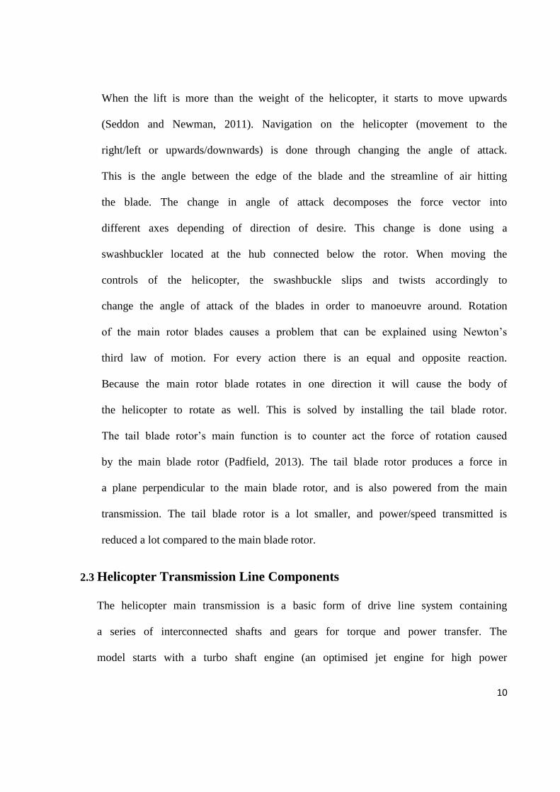
2.3 Helicopter Transmission Line Components

The helicopter main transmission is a basic form of drive line system containing

a series of interconnected shafts and gears for torque and power transfer. The

model starts with a turbo shaft engine (an optimised jet engine for high power

11

and low weight vehicles) rotating at 6000 rpm. This is the source of power that

moves the whole system, and follows the rules of the thermodynamics of a gas

turbine engine that converts energy into torque. The transmission shaft from the

turbo shaft is connected via a series of gear meshes to transmit torque and speed

to rest of the system (Padfield, 2013). The main transmission splits in

functionality to provide torque for both the main rotor and the tail rotor. At both

ends of the transmission lines, the shafts are connected to the hubs and rotary

blades.

Figure 1: Overview of the Components of the Helicopter Transmission System (FAA Safety

Team, Accessed 6 Jan 2019)

2.3.1 Gas Turbine & Turbo shaft

The gas turbine is a form of an internal combustion engine that converts fuel and

air into torque to be used in the transmission. The turbine comprises of 3 main

components: the compressor, the combustion chamber, and the turbine. These 3

components are connected (usually) in one shaft called the rotor. The compressor

12

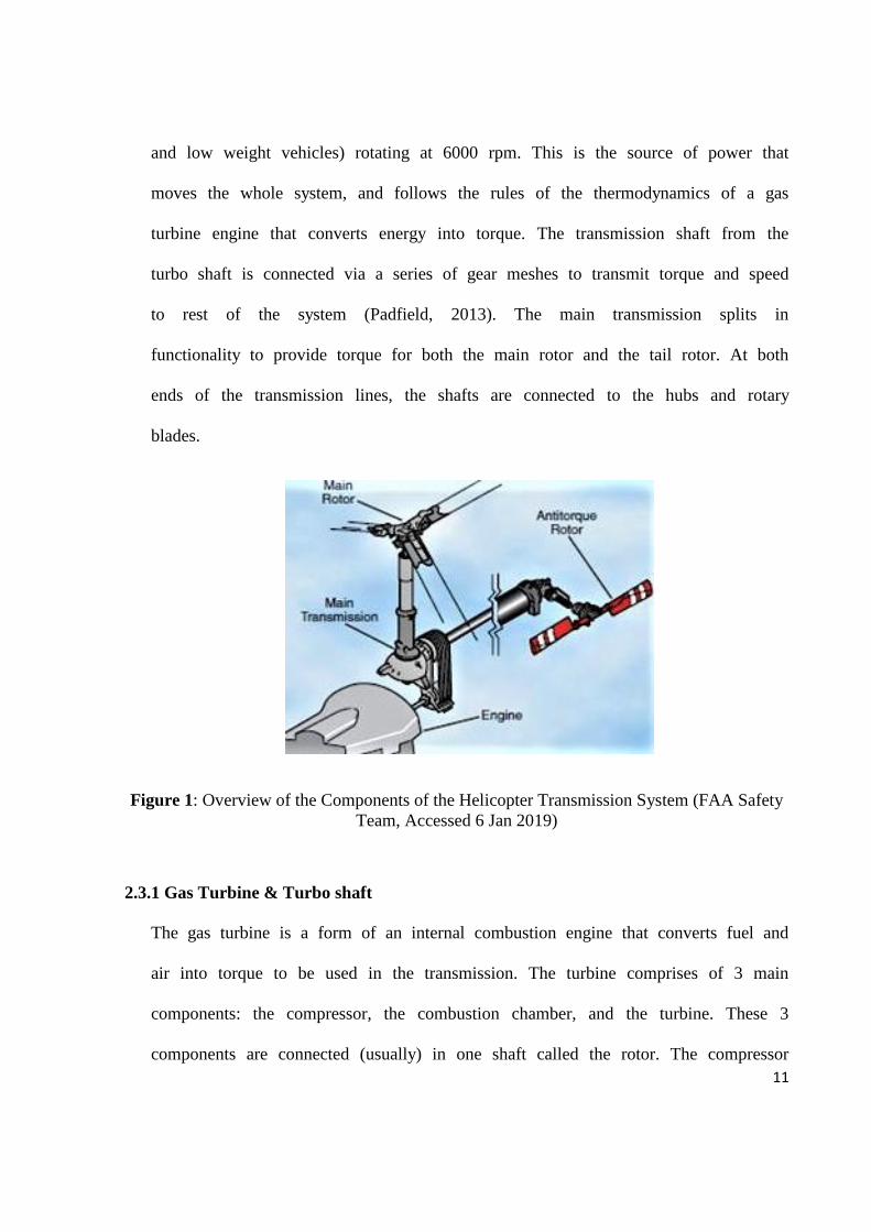
is made of many stages of rotary blades and stationary vanes. These blades and

vanes are in a bent shape named the air foil. The air foils have this specific shape

for a reason, when air travels through the compressor at fast speed, the foils due

to their profile, convert the kinetic energy into pressure energy; increasing the

pressure and temperature of the air (El Naggar, 2015). This process is isentropic

(ideally), meaning there is no heat transfer outside of the system, and reversible,

meaning no losses of energy occurs during the compression. When air exits the

compressor, it enters the combustion chamber, where it mixes with fuel. Inside

the combustion chamber are burners in order to heat the air and fuel mixture to

very high levels of temperature (around 1000 degrees Celsius, depending on gas

turbine operation and type). Combustion is an Isobaric process, meaning it

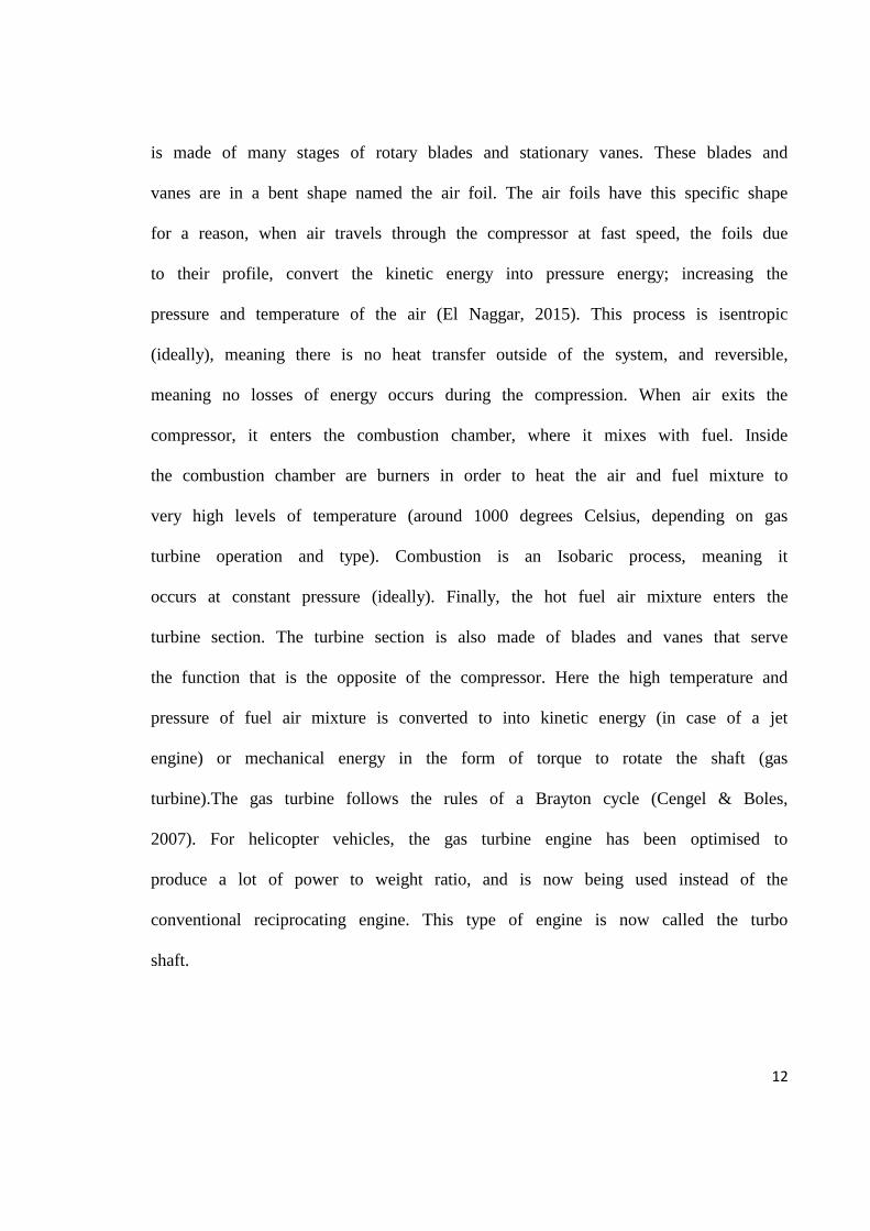
occurs at constant pressure (ideally). Finally, the hot fuel air mixture enters the

turbine section. The turbine section is also made of blades and vanes that serve

the function that is the opposite of the compressor. Here the high temperature and

pressure of fuel air mixture is converted to into kinetic energy (in case of a jet

engine) or mechanical energy in the form of torque to rotate the shaft (gas

turbine).The gas turbine follows the rules of a Brayton cycle (Cengel & Boles,

2007). For helicopter vehicles, the gas turbine engine has been optimised to

produce a lot of power to weight ratio, and is now being used instead of the

conventional reciprocating engine. This type of engine is now called the turbo

shaft.

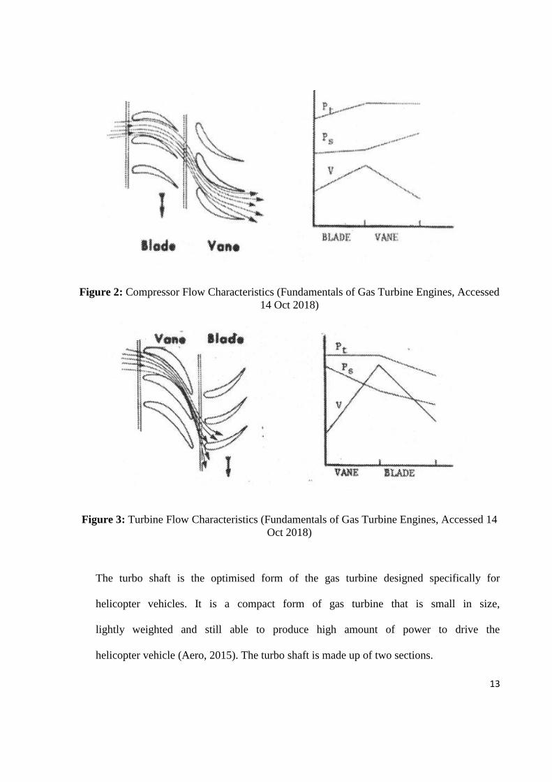
13

Figure 2: Compressor Flow Characteristics (Fundamentals of Gas Turbine Engines, Accessed

14 Oct 2018)

Figure 3: Turbine Flow Characteristics (Fundamentals of Gas Turbine Engines, Accessed 14

Oct 2018)

The turbo shaft is the optimised form of the gas turbine designed specifically for

helicopter vehicles. It is a compact form of gas turbine that is small in size,

lightly weighted and still able to produce high amount of power to drive the

helicopter vehicle (Aero, 2015). The turbo shaft is made up of two sections.

14

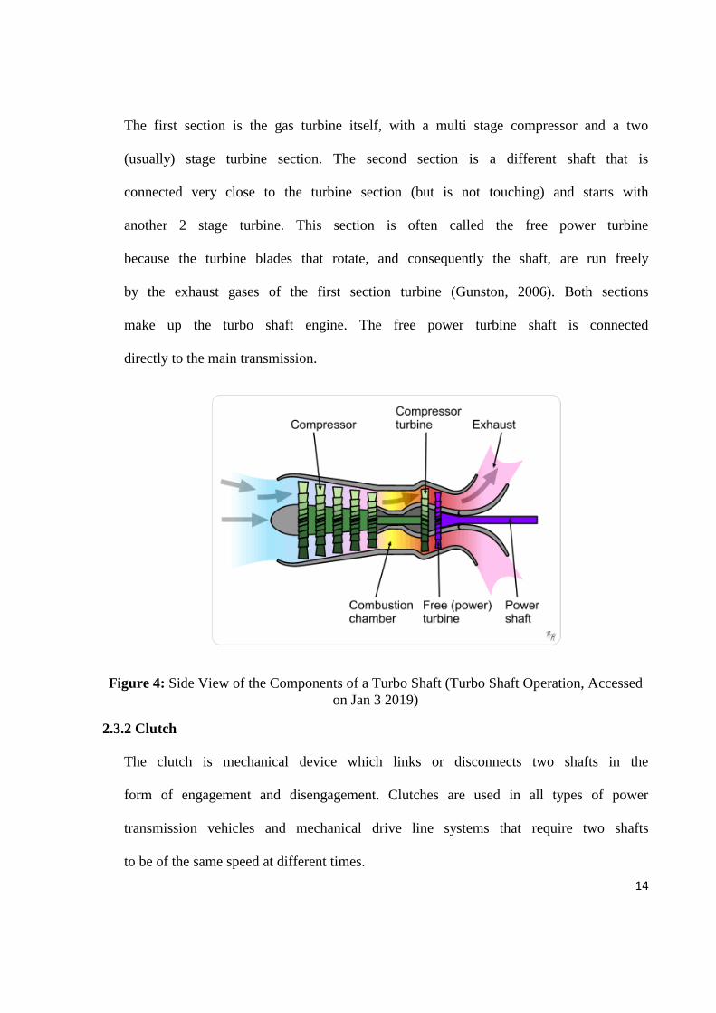
The first section is the gas turbine itself, with a multi stage compressor and a two

(usually) stage turbine section. The second section is a different shaft that is

connected very close to the turbine section (but is not touching) and starts with

another 2 stage turbine. This section is often called the free power turbine

because the turbine blades that rotate, and consequently the shaft, are run freely

by the exhaust gases of the first section turbine (Gunston, 2006). Both sections

make up the turbo shaft engine. The free power turbine shaft is connected

directly to the main transmission.

Figure 4: Side View of the Components of a Turbo Shaft (Turbo Shaft Operation, Accessed

on Jan 3 2019)

2.3.2 Clutch

The clutch is mechanical device which links or disconnects two shafts in the

form of engagement and disengagement. Clutches are used in all types of power

transmission vehicles and mechanical drive line systems that require two shafts

to be of the same speed at different times.

15

Normally, one of the shafts is considered to be the driving shaft and is connected

to a motor or an engine. The other shaft is the driven shaft and is connected to the

output of the system (Padfield, 2013). In helicopter design, there are different

types of clutches developed depending on practicality and feasibility.

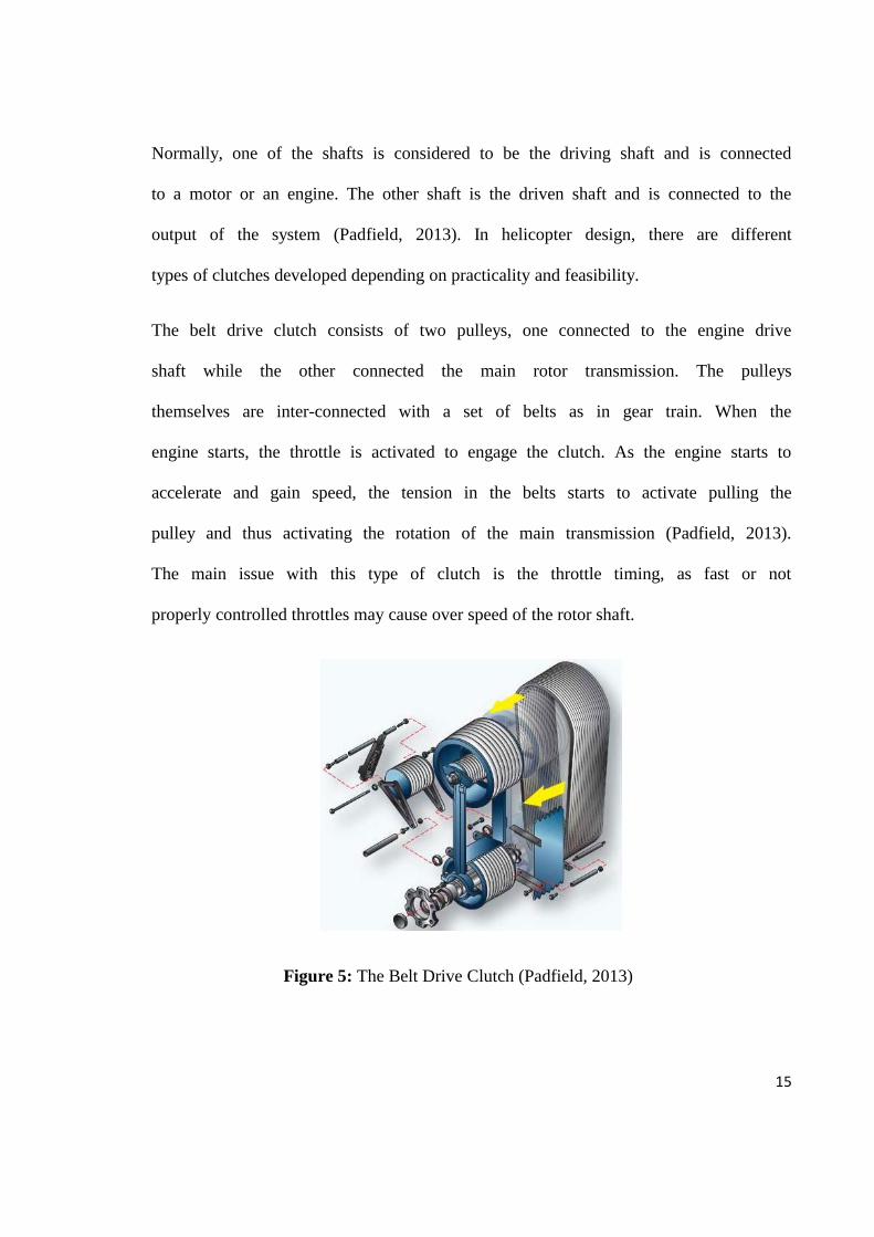
The belt drive clutch consists of two pulleys, one connected to the engine drive

shaft while the other connected the main rotor transmission. The pulleys

themselves are inter-connected with a set of belts as in gear train. When the

engine starts, the throttle is activated to engage the clutch. As the engine starts to

accelerate and gain speed, the tension in the belts starts to activate pulling the

pulley and thus activating the rotation of the main transmission (Padfield, 2013).

The main issue with this type of clutch is the throttle timing, as fast or not

properly controlled throttles may cause over speed of the rotor shaft.

Figure 5: The Belt Drive Clutch (Padfield, 2013)

16

The centrifugal clutch consists of an inner plate and an outer drum. The inner

plate is connected to the drive shaft, while the outer drum is connected to the

main rotor transmission. The inner plate consists of pads similar to break pads

that are held inside by springs. As the rotor speeds up, the centrifugal force of the

pads push the springs outward until the outer drum is touched. This is when the

clutch becomes fully engaged and the rotor drive shaft and driven shaft are

synchronised (Padfield,2013).

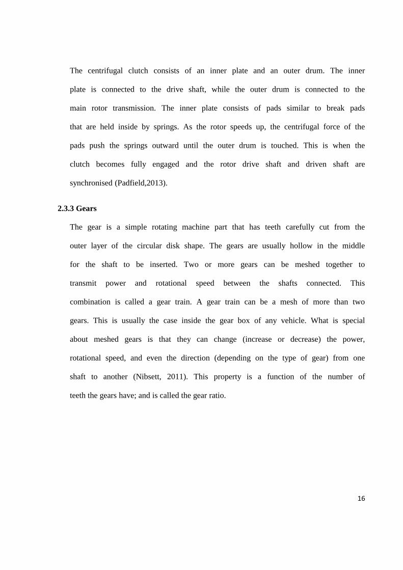
2.3.3 Gears

The gear is a simple rotating machine part that has teeth carefully cut from the

outer layer of the circular disk shape. The gears are usually hollow in the middle

for the shaft to be inserted. Two or more gears can be meshed together to

transmit power and rotational speed between the shafts connected. This

combination is called a gear train. A gear train can be a mesh of more than two

gears. This is usually the case inside the gear box of any vehicle. What is special

about meshed gears is that they can change (increase or decrease) the power,

rotational speed, and even the direction (depending on the type of gear) from one

shaft to another (Nibsett, 2011). This property is a function of the number of

teeth the gears have; and is called the gear ratio.

17

Figure 6: Illustration of a Gear Train (Integrated Publishing, Accessed on Dec 21 2018)

2.4 Lumped Parameter Method

The lumped parameter method is a method derived from analysis of electrical

systems; in electrical systems consisting of resistors, capacitors and inductors. The

lumped parameter method assumes no change in the magnetic field or charge in the

circuit. This results in the Kirchhoff’s laws of electrical circuit analysis. Another

assumption states that the propagation time is less than the period of the signal

inside the circuit (Doebelin, E.O, 1998.). When the propagation time increases to of

a significant value, it must be considered in the analysis and a distributed system

model must be used. In mechanical systems such as the current model (the

helicopter transmission), the method is similar, except it involves rigid bodies of

mechanical parts. The rigid bodies have significant characteristics such as inertia,

mass, dimensions, force and acceleration. These rigid bodies are linked by joints,

clutches, gears. Considering all of these elements as rigid bodies; this means that we

do not study each element as a set of small different parts but one as a whole.

18

We do not consider the temperature, stresses, behavior of each section of the shaft,

but the shaft as a whole. This is what defines a lumped parameter model. In terms of

mathematical modeling, non-linearities in the system are not considered.

2.5 Finite Element Method

The finite element method is a method that sub divides the analyzed system into

small sub sections; thus the name finite elements. Each sub section of the division

will have its own equation model. These equations are then constructed together to

solve the entire problem (K.J.Bathe, 1976). In the helicopter transmission, the shaft

is modeled as a combination of smaller shafts with gears at the end of each sub

section. Equations are modeled for each sub shaft between each two gears. This

creates a series of equations based on the number of sub shafts (or more correctly;

finite elements) taken. The equations themselves are similar to the lumped parameter

model and are dependent on each other. Solving these model equations is difficult

and complex due to the increasing number of the order of the polynomials (after

conversion from differential equations). Software (such as MATLAB) is best used to

avoid calculation errors. The more finite elements taken, the more the system is sub

divided, the higher the order, the higher the difficulty. In the paper “The Torsional

Response of Rotor Systems” the authors applied the finite element method in drive

line systems with 2 rotors by taking 5 to 10 finite elements (Whalley, Ebrahmi,

Jamil, 2005). Results displayed the complexity of the method which gives prone to

inaccuracies.

19

2.6 Impedance Analogy

The impedance analogy is one of the main analogies to describe mechanical systems

as electrical systems; converting the system as whole to easily reach the

mathematical representation model. This analogy is used in the hybrid model

technique, which is derived originally from the transmission line model. Each

element in the mechanical system has a similar and corresponding element in the

electrical system (Dorf, Bishop, 2010).

The mechanical loss of energy due to a resistive force such as friction is what is

known as electrical resistance. The mechanical effect of a damper (or a shock

absorber) is to reduce or dissipate kinetic energy. The corresponding effect of a

resistor is to reduce current flow, or dissipate electrical power.

The shaft itself and the gears have a mass. According to Newton’s first law of

dynamics: when an object (of a certain mass) moves, it continues to move in a

straight line. Thus the object resists the change in velocity, this is called inertia. The

analogous term for the electrical system is inductance. The inductor is a coil

wrapped around an insulator core. When electricity passes through the coil, it creates

a magnetic field around the coil with a direction specified according to Faraday’s

law. When current changes in the coil, this induces an electro motive force in the

coil and this opposes the change in the current. This is resistive property is

analogous to inertia.

20

The stiffness of a rigid body is the resistance to deformation. Since the shaft is

rotating due to torque, the stiffness in this model is mostly used as the resistance to

angular deformation. The weight for the shaft cause a bending stress on the shaft,

and thus the stiffness regards also resistance to linear deformation. This is however

ignored in the model for simplicity and the relation with the topic (not related). The

capacitance is analogous to the inverse of stiffness, which is called, the compliance

(Whalley, Ebrahimi, Jamil, 2005). The capacitor is a component that stores electrical

energy. It is made of two conducting metal plates with a solid insulator in between.

The insulator is referred to as a dielectric solid because of its ability to polarize the

charge passing through; this way the capacitor stores the voltage when charge passes

through.

2.7 Hybrid (Distributed-Lumped) Method

The hybrid method is a method that utilizes both the lumped and distributed

parameters into one representation. This is possible by taking the elements of

interest as a distributed sum, while other elements remain as lumped. In the

helicopter transmission, the shaft stiffness and compliance becomes a function of the

shaft’s properties such as length. Using the transmission line theory, as well as the

impedance analogy, it is possible to compare a mechanical system to an electrical

transmission line. In a long transmission line, the line behaves as a combination of

inductor and capacitor repeated infinitely across the line length. The inductance and

capacitance of this line become partial differential equations that are dependent on

both time and length.

21

These can be accessed from the equations of current and voltage for the inductor and

capacitor. Similarly, in the helicopter transmission, the compliance and stiffness of

the shaft vary across the length (of the shaft) and time. These partial differential

equations can be accessed from the equations of torque and speed. The rest of the

elements of the shaft, such as the mass/inertia of the gears are considered as lumped

parameters. In the paper “The Computational of Torsional, Dynamic Stresses” the

authors applied this method to 2, 3 and derived the equations for multiple rotor

systems (Whalley, Ameer, 2009). The results showed complexity in understanding

the determination of critical speeds.

22

Chapter III: Mathematical Modeling

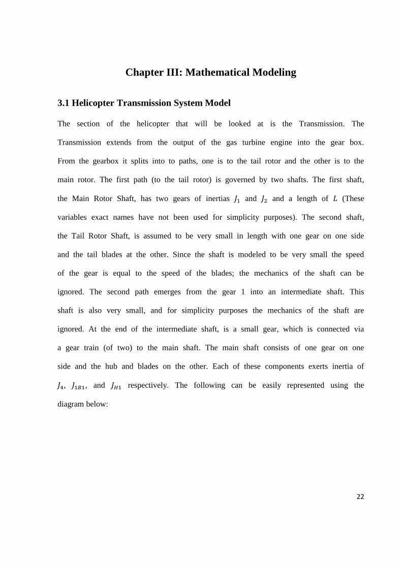
3.1 Helicopter Transmission System Model

The section of the helicopter that will be looked at is the Transmission. The

Transmission extends from the output of the gas turbine engine into the gear box.

From the gearbox it splits into to paths, one is to the tail rotor and the other is to the

main rotor. The first path (to the tail rotor) is governed by two shafts. The first shaft,

the Main Rotor Shaft, has two gears of inertias 𝐽1 and 𝐽2 and a length of 𝐿 (These

variables exact names have not been used for simplicity purposes). The second shaft,

the Tail Rotor Shaft, is assumed to be very small in length with one gear on one side

and the tail blades at the other. Since the shaft is modeled to be very small the speed

of the gear is equal to the speed of the blades; the mechanics of the shaft can be

ignored. The second path emerges from the gear 1 into an intermediate shaft. This

shaft is also very small, and for simplicity purposes the mechanics of the shaft are

ignored. At the end of the intermediate shaft, is a small gear, which is connected via

a gear train (of two) to the main shaft. The main shaft consists of one gear on one

side and the hub and blades on the other. Each of these components exerts inertia of

𝐽4, 𝐽1𝐵1, and 𝐽𝐻1 respectively. The following can be easily represented using the

diagram below:

23

Figure 7: Schematic Model of the Helicopter Transmission System

This model can be analyzed in 3 different ways. These 3 ways can be categorized

into 2 different sections. The first section is the lumped model analysis and the

second section is the distributed model analysis. The distributed model utilizes two

different methods, the finite element method and the hybrid method.

3.2 Lumped Parameter Model

The lump model analysis utilizes each element in the system as discrete figures,

which is what engineers usually do when modeling mechanical elements in a

mechanical system.

24

To simplify the modeling, the system will be cut to different sections in order to

calculate their properties.

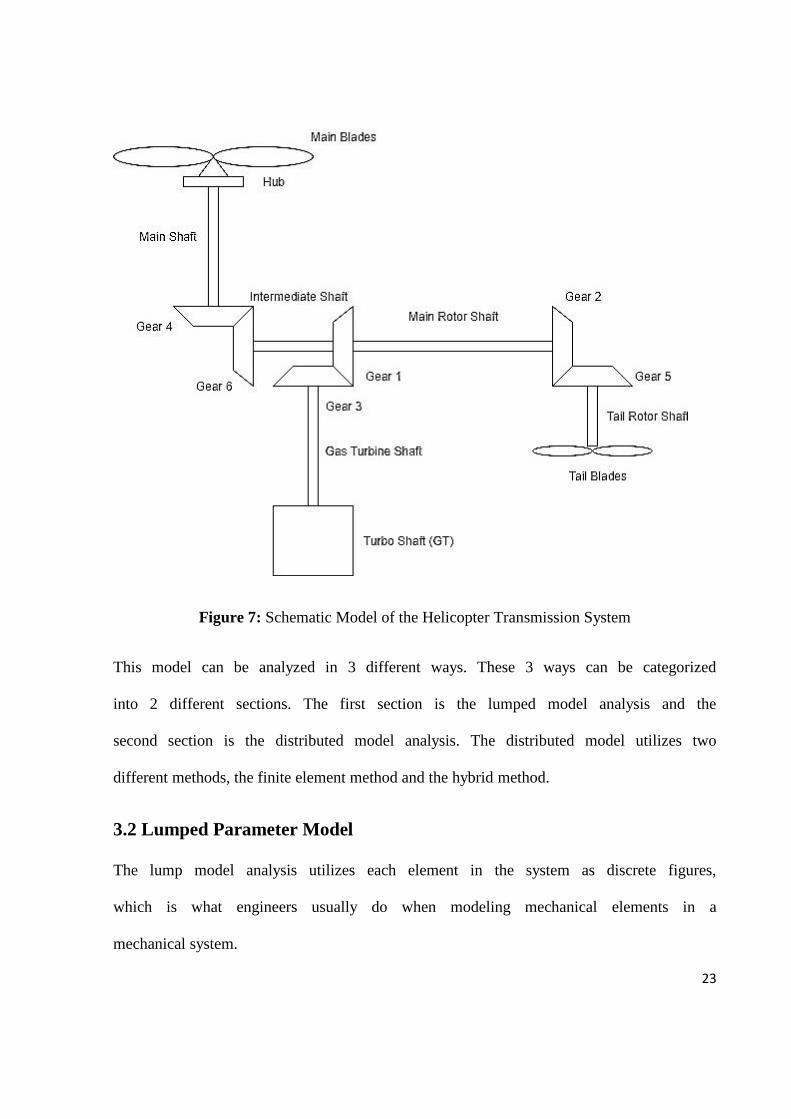
Starting with the Main Rotor Shaft, which is the basis of the whole model (thus the

name).

Figure 8: Main Rotor Shaft (MRS)

The model of this system comes from Newton’s second law of motion, which states:

The sum of the forces acting on an object is equal to the object mass multiplied by

its acceleration.

𝐹 = 𝑚𝑎 (3-1)

Considering this is a system with resistive forces: damping 𝐶 and stiffness 𝐾:

𝐹 – 𝑐𝑣 – 𝑘𝑥 = 𝑚𝑎 (3-2)

Rearranging:

𝐹 = 𝑚𝑎 + 𝑐𝑣 + 𝑘𝑥 (3-3)

Considering acceleration is the derivative of velocity, and velocity itself is the

derivative of displacement, then:

25

𝐹 = 𝑚𝑥’’ + 𝑐𝑥’ + 𝑘𝑥 (3-4)

This is a simple form of the second order differential equation.

However, the concern in our model is not linear displacement, but angular position,

thus turning the equation into:

𝑇 = 𝐽𝜃’’ + 𝑐𝜃’ + 𝑘𝜃 (3-5)

Where T is the Torque acting on the shaft, and J is the mass moment of Inertia of

modeled object.

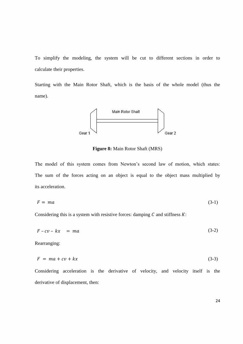
Since the Main Rotor Shaft, has two gears acting on the shaft, in other words, two

forms of inertia (separate), the equation has to be applied on two different point of

axes, at Gear 1 and Gear 2.

Figure 9: Main Rotor Shaft (MRS): Labeled

𝐽1 and 𝐽2 represent the Polar moment of inertia (mass) of gear 1 and gear 2. 𝐶1 and

𝐶2 represent the damping, or the resistance to speed, at each side of the shaft. 𝐾

26

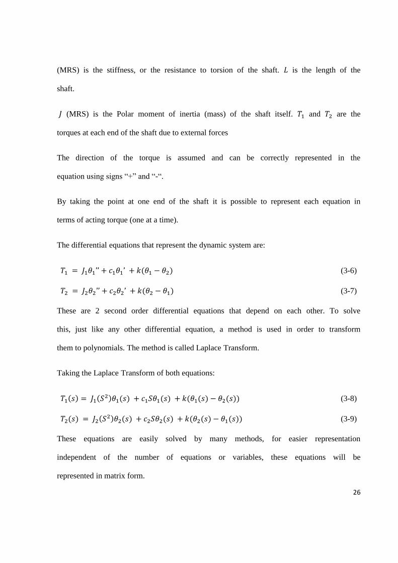
(MRS) is the stiffness, or the resistance to torsion of the shaft. 𝐿 is the length of the

shaft.

𝐽 (MRS) is the Polar moment of inertia (mass) of the shaft itself. 𝑇1 and 𝑇2 are the

torques at each end of the shaft due to external forces

The direction of the torque is assumed and can be correctly represented in the

equation using signs “+” and “-“.

By taking the point at one end of the shaft it is possible to represent each equation in

terms of acting torque (one at a time).

The differential equations that represent the dynamic system are:

𝑇1 = 𝐽1𝜃1’’ + 𝑐1𝜃1’ + 𝑘(𝜃1 − 𝜃2) (3-6)

𝑇2 = 𝐽2𝜃2’’ + 𝑐2𝜃2’ + 𝑘(𝜃2 − 𝜃1) (3-7)

These are 2 second order differential equations that depend on each other. To solve

this, just like any other differential equation, a method is used in order to transform

them to polynomials. The method is called Laplace Transform.

Taking the Laplace Transform of both equations:

𝑇1(𝑠) = 𝐽1(𝑆2)𝜃1(𝑠) + 𝑐1𝑆𝜃1(𝑠) + 𝑘(𝜃1(𝑠) − 𝜃2(𝑠)) (3-8)

𝑇2(𝑠) = 𝐽2(𝑆2)𝜃2(𝑠) + 𝑐2𝑆𝜃2(𝑠) + 𝑘(𝜃2(𝑠) − 𝜃1(𝑠)) (3-9)

These equations are easily solved by many methods, for easier representation

independent of the number of equations or variables, these equations will be

represented in matrix form.

27

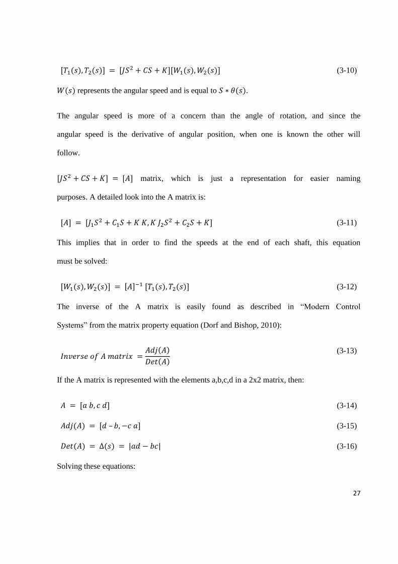
[𝑇1(𝑠), 𝑇2(𝑠)] = [𝐽𝑆2 + 𝐶𝑆 + 𝐾][𝑊1(𝑠), 𝑊2(𝑠)] (3-10)

𝑊(𝑠) represents the angular speed and is equal to 𝑆 ∗ 𝜃(𝑠).

The angular speed is more of a concern than the angle of rotation, and since the

angular speed is the derivative of angular position, when one is known the other will

follow.

[𝐽𝑆2 + 𝐶𝑆 + 𝐾] = [𝐴] matrix, which is just a representation for easier naming

purposes. A detailed look into the A matrix is:

[𝐴] = [𝐽1𝑆2 + 𝐶1𝑆 + 𝐾 𝐾, 𝐾 𝐽2𝑆2 + 𝐶2𝑆 + 𝐾] (3-11)

This implies that in order to find the speeds at the end of each shaft, this equation

must be solved:

[𝑊1(𝑠), 𝑊2(𝑠)] = [𝐴]−1 [𝑇1(𝑠), 𝑇2(𝑠)] (3-12)

The inverse of the A matrix is easily found as described in “Modern Control

Systems” from the matrix property equation (Dorf and Bishop, 2010):

𝐼𝑛𝑣𝑒𝑟𝑠𝑒 𝑜𝑓 𝐴 𝑚𝑎𝑡𝑟𝑖𝑥 =𝐴𝑑𝑗(𝐴)

𝐷𝑒𝑡(𝐴)

(3-13)

If the A matrix is represented with the elements a,b,c,d in a 2x2 matrix, then:

𝐴 = [𝑎 𝑏, 𝑐 𝑑] (3-14)

𝐴𝑑𝑗(𝐴) = [𝑑 – 𝑏, −𝑐 𝑎] (3-15)

𝐷𝑒𝑡(𝐴) = ∆(𝑠) = |𝑎𝑑 − 𝑏𝑐| (3-16)

Solving these equations:

28

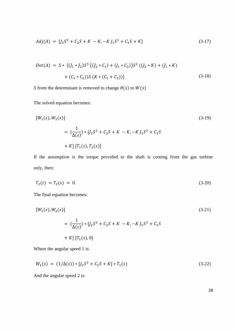
𝐴𝑑𝑗(𝐴) = [𝐽2𝑆2 + 𝐶2𝑆 + 𝐾 − 𝐾, −𝐾 𝐽1𝑆2 + 𝐶1𝑆 + 𝐾] (3-17)

𝐷𝑒𝑡(𝐴) = 𝑆 ∗ [(𝐽1 ∗ 𝐽2)𝑆3 ((𝐽2 ∗ 𝐶1) + (𝐽1 ∗ 𝐶2))𝑆2 ((𝐽2 ∗ 𝐾) + (𝐽1 ∗ 𝐾)

+ (𝐶1 ∗ 𝐶2))𝑆 (𝐾 ∗ (𝐶1 + 𝐶2))]

(3-18)

𝑆 from the determinant is removed to change 𝜃(𝑠) to 𝑊(𝑠)

The solved equation becomes:

[𝑊1(𝑠), 𝑊2(𝑠)]

= (1

∆(𝑠)) ∗ [𝐽2𝑆2 + 𝐶2𝑆 + 𝐾 − 𝐾, −𝐾 𝐽1𝑆2 + 𝐶1𝑆

+ 𝐾] [𝑇1(𝑠), 𝑇2(𝑠)]

(3-19)

If the assumption is the torque provided to the shaft is coming from the gas turbine

only, then:

𝑇2(𝑡) = 𝑇2(𝑠) = 0. (3-20)

The final equation becomes:

[𝑊1(𝑠), 𝑊2(𝑠)]

= (1

∆(𝑠)) ∗ [𝐽2𝑆2 + 𝐶2𝑆 + 𝐾 − 𝐾, −𝐾 𝐽1𝑆2 + 𝐶1𝑆

+ 𝐾] [𝑇1(𝑠), 0]

(3-21)

Where the angular speed 1 is:

𝑊1(𝑠) = (1/∆(𝑠)) ∗ [𝐽2𝑆2 + 𝐶2𝑆 + 𝐾] ∗ 𝑇1(𝑠) (3-22)

And the angular speed 2 is:

29

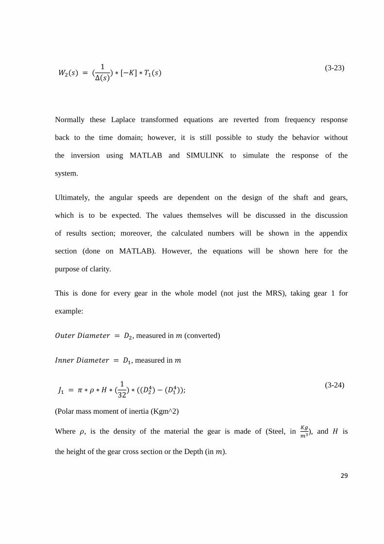
𝑊2(𝑠) = (1

∆(𝑠)) ∗ [−𝐾] ∗ 𝑇1(𝑠)

(3-23)

Normally these Laplace transformed equations are reverted from frequency response

back to the time domain; however, it is still possible to study the behavior without

the inversion using MATLAB and SIMULINK to simulate the response of the

system.

Ultimately, the angular speeds are dependent on the design of the shaft and gears,

which is to be expected. The values themselves will be discussed in the discussion

of results section; moreover, the calculated numbers will be shown in the appendix

section (done on MATLAB). However, the equations will be shown here for the

purpose of clarity.

This is done for every gear in the whole model (not just the MRS), taking gear 1 for

example:

𝑂𝑢𝑡𝑒𝑟 𝐷𝑖𝑎𝑚𝑒𝑡𝑒𝑟 = 𝐷2, measured in 𝑚 (converted)

𝐼𝑛𝑛𝑒𝑟 𝐷𝑖𝑎𝑚𝑒𝑡𝑒𝑟 = 𝐷1, measured in 𝑚

𝐽1 = 𝜋 ∗ 𝜌 ∗ 𝐻 ∗ (1

32) ∗ ((𝐷2

4) − (𝐷14));

(3-24)

(Polar mass moment of inertia (Kgm^2)

Where 𝜌, is the density of the material the gear is made of (Steel, in 𝐾𝑔

𝑚3), and 𝐻 is

the height of the gear cross section or the Depth (in 𝑚).

30

The same way, 𝐽2 and 𝐽𝑀𝑅𝑆 are calculated.

𝐶, the damping, is assumed from practice (in 𝑁

𝑚)

𝐾, the stiffness of the shaft is calculated:

𝐾 = 𝐺 ∗𝐽

𝐿

(3-25)

However, due to the fact that stiffness is independent mass, J here is Polar moment

of inertia not the Polar mass moment of inertia, the equation must be adjusted for

consistency.

The equation becomes:

𝐾 =𝐺 ∗ 𝐽

𝜌 ∗ (𝐿2 )

(3-26)

Where 𝐺 is the modulus of rigidity, which is dependent on the shaft material (Steel,

in 𝑁/𝑚2).

𝐽 is Polar mass moment of inertia of the shaft.

𝜌 is the density of the material.

𝐿 is the length of the shaft.

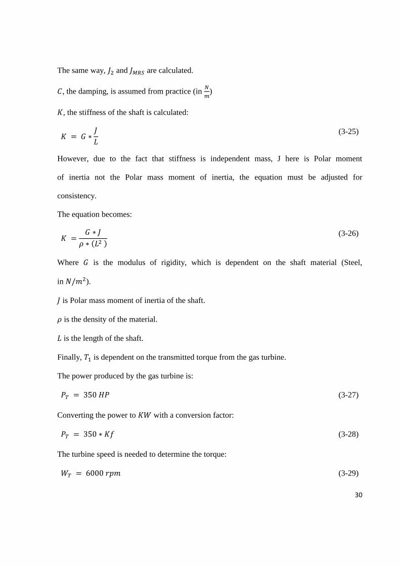
Finally, 𝑇1 is dependent on the transmitted torque from the gas turbine.

The power produced by the gas turbine is:

𝑃𝑇 = 350 𝐻𝑃 (3-27)

Converting the power to 𝐾𝑊 with a conversion factor:

𝑃𝑇 = 350 ∗ 𝐾𝑓 (3-28)

The turbine speed is needed to determine the torque:

𝑊𝑇 = 6000 𝑟𝑝𝑚 (3-29)

31

Again, the angular speed of the turbine is converted to 𝐻𝑧 with a conversion factor:

𝑊𝑇 = 6000 ∗ 𝐾ℎ (3-30)

The Torque produced on the gas turbine shaft is:

𝑇𝑇 = 𝑃𝑇/𝑊𝑇 = (350

6000) ∗ (

𝐾𝑓

𝐾ℎ)

(3-31)

The Gear Ratio between Gear 3 and Gear 1 determines the torque transmitted to the

Main Rotor Shaft, 𝑇1.

The Gear Ratio between Gear 3 and 1 is:

𝐺𝑅1 =𝑁3

𝑁1

(3-32)

Where 𝑁3 and 𝑁1 are the number of teeth of gear 3 and gear 1 respectively.

Finally, the torque on Main Rotor Shaft is:

𝑇1 = (350

6000) ∗ (

𝐾𝑓

𝐾ℎ) ∗ (

𝑁3

𝑁1)

(3-33)

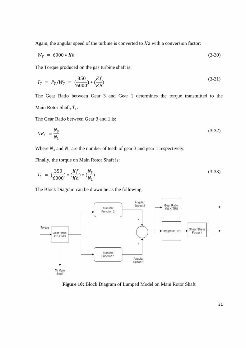
The Block Diagram can be drawn be as the following:

Figure 10: Block Diagram of Lumped Model on Main Rotor Shaft

32

Equations of Transfer functions used in SIMULINK and MATLAB can be found in

the

33

Appendix I.

On the Main Shaft, the analysis is very similar to the Main Rotor Shaft with the

exception of the inertia. Instead of two gears at two ends, it is one gear at one end

and blades + Hub on the other end.

The equation of the Main Shaft becomes:

[𝑊4(𝑠), 𝑊𝐵1(𝑠)]

= (1

∆(𝑠)) ∗ [𝐽𝐵1𝑆2 + 𝐶𝐵1𝑆 + 𝐾2 – 𝐾2, −𝐾2 𝐽4𝑆2 + 𝐶4𝑆

+ 𝐾2] [𝑇4(𝑠), 0]

(3-34)

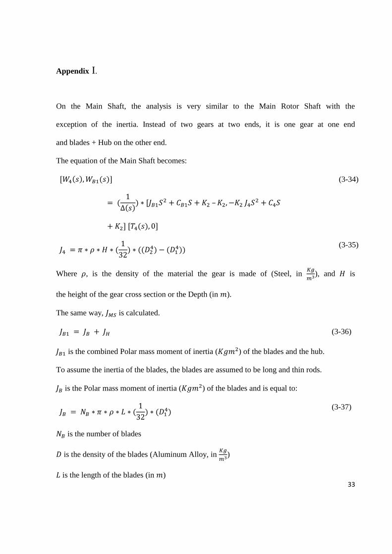
𝐽4 = 𝜋 ∗ 𝜌 ∗ 𝐻 ∗ (1

32) ∗ ((𝐷2

4) − (𝐷14))

(3-35)

Where 𝜌, is the density of the material the gear is made of (Steel, in 𝐾𝑔

𝑚3), and 𝐻 is

the height of the gear cross section or the Depth (in 𝑚).

The same way, 𝐽𝑀𝑆 is calculated.

𝐽𝐵1 = 𝐽𝐵 + 𝐽𝐻 (3-36)

𝐽𝐵1 is the combined Polar mass moment of inertia (𝐾𝑔𝑚2) of the blades and the hub.

To assume the inertia of the blades, the blades are assumed to be long and thin rods.

𝐽𝐵 is the Polar mass moment of inertia (𝐾𝑔𝑚2) of the blades and is equal to:

𝐽𝐵 = 𝑁𝐵 ∗ 𝜋 ∗ 𝜌 ∗ 𝐿 ∗ (1

32) ∗ (𝐷1

4) (3-37)

𝑁𝐵 is the number of blades

𝐷 is the density of the blades (Aluminum Alloy, in 𝐾𝑔

𝑚3)

𝐿 is the length of the blades (in 𝑚)

34

𝐷1 is the diameter of the blades (assumed as rods, in m)

The hub is then calculated to be:

𝐽𝐻 = 𝜋 ∗ 𝜌 ∗ 𝐿 ∗ (1

32) ∗ (𝐷4)

(3-38)

In which the variables represent the same characteristics but for the hub.

𝐶, the damping, is assumed from practice (in N/m)

𝐾2, the stiffness of the shaft is calculated from:

𝐾2 =𝐺 ∗ 𝐽

𝜌 ∗ (𝐿2 )

(3-39)

𝑇4, is the torque at the Main Shaft and is equal to:

𝑇4 = (350

6000) ∗ (

𝐾𝑓

𝐾ℎ) ∗ (

𝑁3

𝑁1) ∗ (

𝑁6

𝑁4)

(3-40)

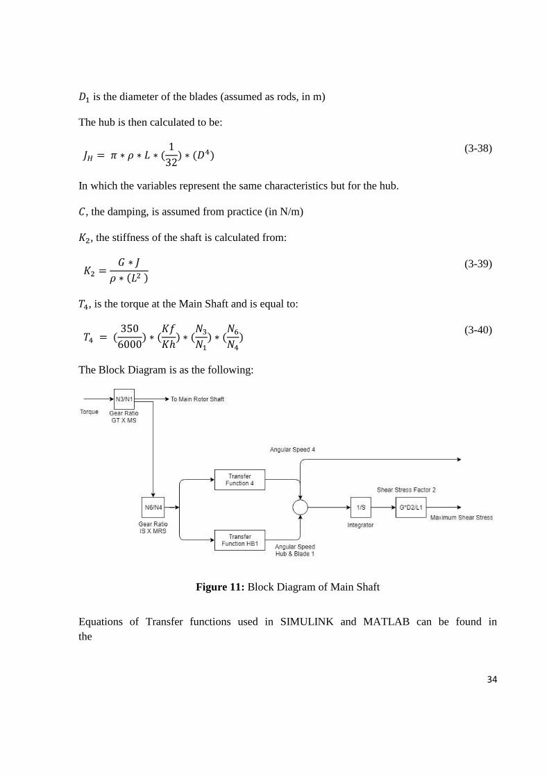
The Block Diagram is as the following:

Figure 11: Block Diagram of Main Shaft


the

35

Appendix I.

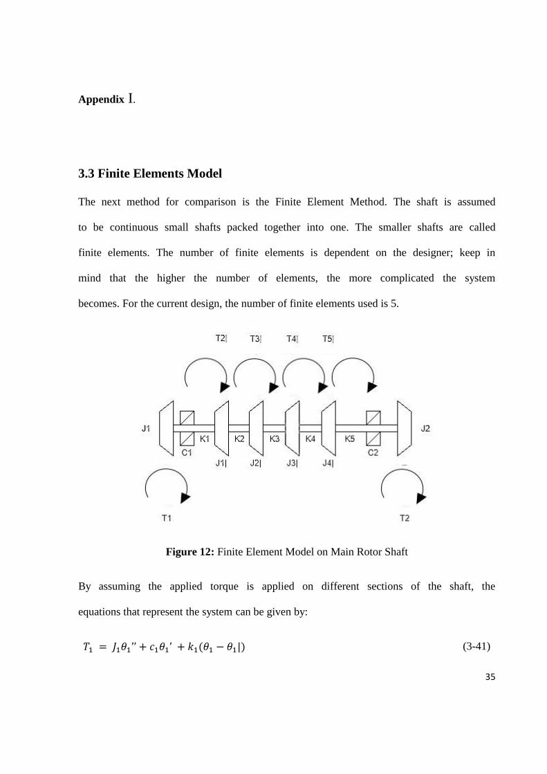
3.3 Finite Elements Model

The next method for comparison is the Finite Element Method. The shaft is assumed

to be continuous small shafts packed together into one. The smaller shafts are called

finite elements. The number of finite elements is dependent on the designer; keep in

mind that the higher the number of elements, the more complicated the system

becomes. For the current design, the number of finite elements used is 5.

Figure 12: Finite Element Model on Main Rotor Shaft

By assuming the applied torque is applied on different sections of the shaft, the

equations that represent the system can be given by:

𝑇1 = 𝐽1𝜃1’’ + 𝑐1𝜃1’ + 𝑘1(𝜃1 − 𝜃1|) (3-41)

36

𝑇2| = 𝐽1|𝜃1|’’ + 𝑘1(𝜃1| − 𝜃1) + 𝑘2(𝜃1| − 𝜃2|) (3-41)

𝑇3| = 𝐽2|𝜃2|’’ + 𝑘2(𝜃2| − 𝜃1|) + 𝑘3(𝜃2| − 𝜃3|) (3-42)

𝑇4| = 𝐽3|𝜃3|’’ + 𝑘3(𝜃3| − 𝜃2|) + 𝑘4(𝜃3| − 𝜃4|) (3-34)

𝑇 5

|= 𝐽4|𝜃4|’’ + 𝑘4(𝜃4| − 𝜃3|) + 𝑘5(𝜃4| − 𝜃2) (3-44)

𝑇6| = 𝐽2𝜃2’’ + 𝑐2𝜃2’ + 𝑘5(𝜃2 − 𝜃4|) (3-45)

Since the torque is coming from the gas turbine only:

𝑇2| = 𝑇3| = 𝑇4| = 𝑇5| = 𝑇6| = 0 (3-46)

The finite elements are assumed to be equal:

The polar moment of inertia of the elements is:

𝐽1 = 𝐽2 = 𝐽3 = 𝐽4 = 𝐽 (3-47)

Where the inertia of the 5 elements is equal to:

𝐽 =𝐽𝑀𝑅𝑆

5

(3-48)

The stiffness of the shaft between each element is represented in the model, making

the combined stiffness to be:

𝐾 = 𝑘1 + 𝑘2 + 𝑘3 + 𝑘4 + 𝑘5 (3-9)

The stiffness between each element is also assumed to be equal:

𝑘1 = 𝑘2 = 𝑘3 = 𝑘4 = 𝑘5 = 𝑘 (3-10)

The total stiffness of the shaft increases, and is equal to:

𝐾 = 5 ∗ 𝑘 (3-11)

37

On the other hand the length between each element is:

𝐿| =𝐿

5

(3-12)

Taking the Laplace transform of the equations:

𝑇1(𝑠) = 𝐽1(𝑆2)𝜃1(𝑠) + 𝑐1(𝑆)𝜃1(𝑠) + 𝑘1(𝜃1(𝑠) − 𝜃1|(𝑠)) (3-13)

0 = 𝐽1|(𝑆2)𝜃1|(𝑠) + 𝑘1(𝜃1|(𝑠) − 𝜃1(𝑠)) + 𝑘2(𝜃1|(𝑠) − 𝜃2|(𝑠)) (3-14)

0 = 𝐽2|(𝑆2)𝜃2|(𝑠) + 𝑘2(𝜃2|(𝑠) − 𝜃1|(𝑠)) + 𝑘3(𝜃2|(𝑠) − 𝜃3|(𝑠)) (3-15)

0 = 𝐽3|(𝑆2)𝜃3|(𝑠) + 𝑘3(𝜃3|(𝑠) − 𝜃2|(𝑠)) + 𝑘4(𝜃3|(𝑠) − 𝜃4|(𝑠)) (3-16)

0 = 𝐽4|(𝑆2)𝜃4|(𝑠) + 𝑘4(𝜃4|(𝑠) − 𝜃3|(𝑠)) + 𝑘5(𝜃4|(𝑠) − 𝜃2(𝑠)) (3-17)

0 = 𝐽2(𝑆2)𝜃2(𝑠) + 𝑐2(𝑆)𝜃2(𝑠) + 𝑘5(𝜃2(𝑠) − 𝜃4|(𝑠)) (3-18)

These 6 equations represent the mechanics of the Main Rotor Shaft Taking the

matrix from of the equations, (Whalley, Ebrahimi and Jamil, 2005):

[𝑇1(𝑠), 0, 0, 0, 0, 0]

= [𝐽(𝑆2) + 𝐶(𝑆) + 𝐾]

∗ [𝜃1(𝑠), 𝜃1|(𝑠 ), 𝜃2|(𝑠), 𝜃3|(𝑠), 𝜃4|(𝑠), 𝜃2(𝑠)]

(3-19)

Since 𝑆 ∗ 𝜃(𝑠) = 𝑊(𝑆), the [𝐽(𝑆2) + 𝐶(𝑆) + 𝐾] is just multiplied by 𝑆, in which 𝐷𝑒𝑙𝑡𝑎(𝑆)

will be of 1 lower power.

This does not change the equation:

38

[𝑇1(𝑠), 0, 0, 0, 0, 0]

= [𝐽(𝑆2) + 𝐶(𝑆) + 𝐾]

∗ [𝑊1(𝑠), 𝑊1|(𝑠), 𝑊2|(𝑠), 𝑊3|(𝑠), 𝑊4|(𝑠), 𝑊2(𝑠)]

(3-20)

The angular speeds of the finite elements is not to be concerned about, as the main

objective is to compare speeds of the ends of the shaft 𝑊1 and 𝑊2 to other models.

Matrix A is again made to be:

[𝐴] = [𝐽(𝑆2) + 𝐶(𝑆) + 𝐾] (3-21)

Where the Polar moment of inertia matrix is equal to:

[𝐽] = [𝐽1 0 0 0 0 0, 0 𝐽 0 0 0 0, 0 0 𝐽 0 0 0, 0 0 0 𝐽 0 0, 0 0 0 0 𝐽 0, 0 0 0 0 0 𝐽2] (3-22)

The damping matrix is:

[𝐶]

= [𝐶1 0 0 0 0 0, 0 0 0 0 0 0, 0 0 0 0 0 0, 0 0 0 0 0 0, 0 0 0 0 0 0, 0 0 0 0 0 𝐶2]

(3-23)

The stiffness is matrix is:

[𝐾] = [𝑘 − 𝑘 0 0 0 0, −𝑘 2𝑘 − 𝑘 0 0 0, 0 − 𝑘 2𝑘 − 𝑘 0 0, 0 0 − 𝑘 2𝑘 −

𝑘 0, 0 0 0 − 𝑘 2𝑘 − 𝑘, 0 0 0 0 − 𝑘 𝑘]

(3-24)

The equation of the model now becomes:

[𝑊1(𝑠), 𝑊1|(𝑠), 𝑊2|(𝑠), 𝑊3|(𝑠), 𝑊4|(𝑠), 𝑊2(𝑠)] = [𝐴]−1 ∗ [𝑇1(𝑠), 0, 0, 0, 0, 0] (3-25)

Where the inverse matrix of A is equal to:

39

[𝐴]−1 =𝐴𝑑𝑗

𝐷𝑒𝑡

(3-26)

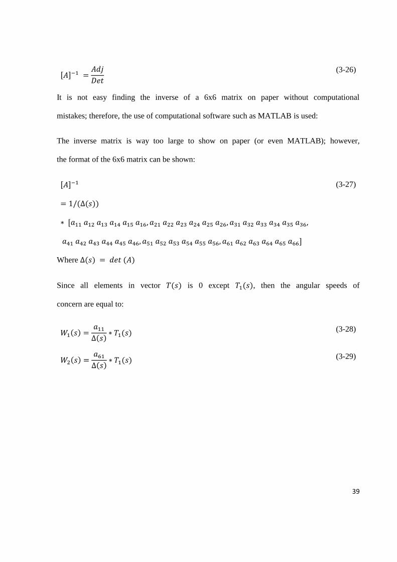
It is not easy finding the inverse of a 6x6 matrix on paper without computational

mistakes; therefore, the use of computational software such as MATLAB is used:

The inverse matrix is way too large to show on paper (or even MATLAB); however,

the format of the 6x6 matrix can be shown:

[𝐴]−1

= 1/(∆(𝑠))

∗ [𝑎11 𝑎12 𝑎13 𝑎14 𝑎15 𝑎16, 𝑎21 𝑎22 𝑎23 𝑎24 𝑎25 𝑎26, 𝑎31 𝑎32 𝑎33 𝑎34 𝑎35 𝑎36,

𝑎41 𝑎42 𝑎43 𝑎44 𝑎45 𝑎46, 𝑎51 𝑎52 𝑎53 𝑎54 𝑎55 𝑎56, 𝑎61 𝑎62 𝑎63 𝑎64 𝑎65 𝑎66]

(3-27)

Where ∆(𝑠) = 𝑑𝑒𝑡 (𝐴)

Since all elements in vector 𝑇(𝑠) is 0 except 𝑇1(𝑠), then the angular speeds of

concern are equal to:

𝑊1(𝑠) =𝑎11

∆(𝑠)∗ 𝑇1(𝑠) (3-28)

𝑊2(𝑠) =𝑎61

∆(𝑠)∗ 𝑇1(𝑠) (3-29)

40

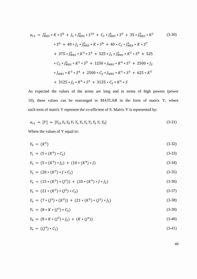
𝑎11 = 𝐽𝑀𝑅𝑆4 ∗ 𝐾 ∗ 𝑆8 + 𝐽2 ∗ 𝐽𝑀𝑅𝑆

4 ∗ 𝑆10 + 𝐶2 ∗ 𝐽𝑀𝑅𝑆4 ∗ 𝑆9 + 35 ∗ 𝐽𝑀𝑅𝑆

3 ∗ 𝐾2

∗ 𝑆6 + 40 ∗ 𝐽2 ∗ 𝐽𝑀𝑅𝑆3 ∗ 𝐾 ∗ 𝑆8 + 40 ∗ 𝐶2 ∗ 𝐽𝑀𝑅𝑆

3 ∗ 𝐾 ∗ 𝑆7

+ 375 ∗ 𝐽𝑀𝑅𝑆2 ∗ 𝐾3 ∗ 𝑆4 + 525 ∗ 𝐽2 ∗ 𝐽𝑀𝑅𝑆

2 ∗ 𝐾2 ∗ 𝑆6 + 525

∗ 𝐶2 ∗ 𝐽𝑀𝑅𝑆2 ∗ 𝐾2 ∗ 𝑆5 + 1250 ∗ 𝐽𝑀𝑅𝑆 ∗ 𝐾4 ∗ 𝑆2 + 2500 ∗ 𝐽2

∗ 𝐽𝑀𝑅𝑆 ∗ 𝐾3 ∗ 𝑆4 + 2500 ∗ 𝐶2 ∗ 𝐽𝑀𝑅𝑆 ∗ 𝐾3 ∗ 𝑆3 + 625 ∗ 𝐾5

+ 3125 ∗ 𝐽2 ∗ 𝐾4 ∗ 𝑆2 + 3125 ∗ 𝐶2 ∗ 𝐾4 ∗ 𝑆

(3-30)

As expected the values of the terms are long and in terms of high powers (power

10), these values can be rearranged in MATLAB in the form of matrix Y, where

each term of matrix Y represent the co-efficient of S. Matrix Y is represented by:

𝑎11 = [𝑌] = [𝑌10 𝑌9 𝑌8 𝑌7 𝑌6 𝑌5 𝑌4 𝑌3 𝑌2 𝑌1 𝑌0] (3-31)

Where the values of Y equal to:

𝑌0 = (𝐾5) (3-32)

𝑌1 = (5 ∗ (𝐾4) ∗ 𝐶2) (3-33)

𝑌2 = (5 ∗ (𝐾4) ∗ 𝐽2) + (10 ∗ (𝐾4) ∗ 𝐽) (3-34)

𝑌3 = (20 ∗ (𝐾3) ∗ 𝐽 ∗ 𝐶2) (3-35)

𝑌4 = (15 ∗ (𝐾3) ∗ (𝐽2)) + (20 ∗ (𝐾3) ∗ 𝐽 ∗ 𝐽2) (3-36)

𝑌5 = (21 ∗ (𝐾2) ∗ (𝐽2) ∗ 𝐶2) (3-37)

𝑌6 = (7 ∗ (𝐽3) ∗ (𝐾2)) + (21 ∗ (𝐾2) ∗ (𝐽2) ∗ 𝐽2) (3-38)

𝑌7 = (8 ∗ 𝐾 ∗ (𝐽3) ∗ 𝐶2) (3-39)

𝑌8 = (8 ∗ 𝐾 ∗ (𝐽3) ∗ 𝐽2) + (𝐾 ∗ (𝐽4)) (3-40)

𝑌9 = ((𝐽4) ∗ 𝐶2) (3-41)

41

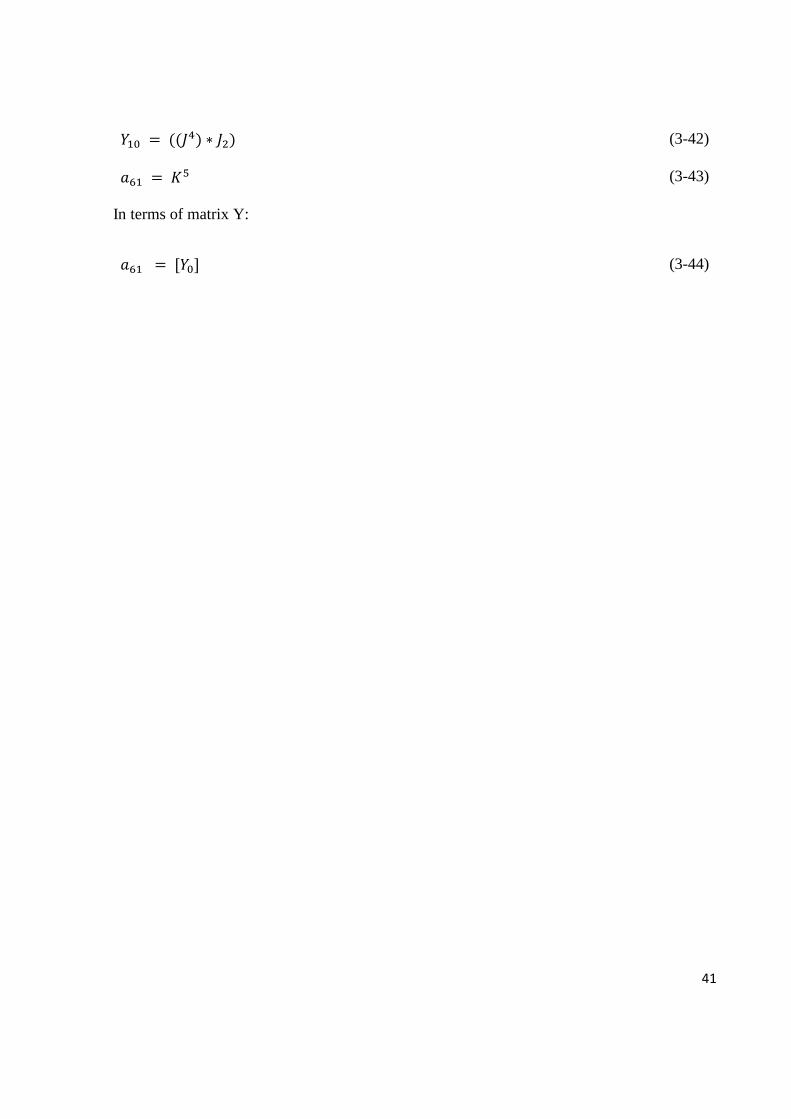
𝑌10 = ((𝐽4) ∗ 𝐽2) (3-42)

𝑎61 = 𝐾5 (3-43)

In terms of matrix Y:

𝑎61 = [𝑌0] (3-44)

42

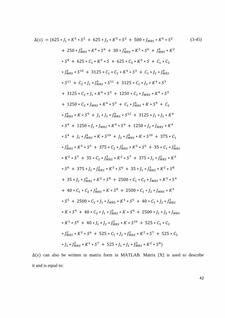
∆(𝑠) = (625 ∗ 𝐽1 ∗ 𝐾5 ∗ 𝑆2 + 625 ∗ 𝐽2 ∗ 𝐾5 ∗ 𝑆2 + 500 ∗ 𝐽𝑀𝑅𝑆 ∗ 𝐾5 ∗ 𝑆2

+ 250 ∗ 𝐽𝑀𝑅𝑆2 ∗ 𝐾4 ∗ 𝑆4 + 30 ∗ 𝐽𝑀𝑅𝑆

3 ∗ 𝐾3 ∗ 𝑆6 + 𝐽𝑀𝑅𝑆4 ∗ 𝐾2

∗ 𝑆8 + 625 ∗ 𝐶1 ∗ 𝐾5 ∗ 𝑆 + 625 ∗ 𝐶2 ∗ 𝐾5 ∗ 𝑆 + 𝐶1 ∗ 𝐶2

∗ 𝐽𝑀𝑅𝑆4 ∗ 𝑆10 + 3125 ∗ 𝐶1 ∗ 𝐶2 ∗ 𝐾4 ∗ 𝑆2 + 𝐶1 ∗ 𝐽2 ∗ 𝐽𝑀𝑅𝑆

4

∗ 𝑆11 + 𝐶2 ∗ 𝐽1 ∗ 𝐽𝑀𝑅𝑆4 ∗ 𝑆11 + 3125 ∗ 𝐶1 ∗ 𝐽2 ∗ 𝐾4 ∗ 𝑆3

+ 3125 ∗ 𝐶2 ∗ 𝐽1 ∗ 𝐾4 ∗ 𝑆3 + 1250 ∗ 𝐶1 ∗ 𝐽𝑀𝑅𝑆 ∗ 𝐾4 ∗ 𝑆3

+ 1250 ∗ 𝐶2 ∗ 𝐽𝑀𝑅𝑆 ∗ 𝐾4 ∗ 𝑆3 + 𝐶1 ∗ 𝐽𝑀𝑅𝑆4 ∗ 𝐾 ∗ 𝑆9 + 𝐶2

∗ 𝐽𝑀𝑅𝑆4 ∗ 𝐾 ∗ 𝑆9 + 𝐽1 ∗ 𝐽2 ∗ 𝐽𝑀𝑅𝑆

4 ∗ 𝑆12 + 3125 ∗ 𝐽1 ∗ 𝐽2 ∗ 𝐾4

∗ 𝑆4 + 1250 ∗ 𝐽1 ∗ 𝐽𝑀𝑅𝑆 ∗ 𝐾4 ∗ 𝑆4 + 1250 ∗ 𝐽2 ∗ 𝐽𝑀𝑅𝑆 ∗ 𝐾4

∗ 𝑆4 + 𝐽1 ∗ 𝐽𝑀𝑅𝑆4 ∗ 𝐾 ∗ 𝑆10 + 𝐽2 ∗ 𝐽𝑀𝑅𝑆

4 ∗ 𝐾 ∗ 𝑆10 + 375 ∗ 𝐶1

∗ 𝐽𝑀𝑅𝑆2 ∗ 𝐾3 ∗ 𝑆5 + 375 ∗ 𝐶2 ∗ 𝐽𝑀𝑅𝑆

2 ∗ 𝐾3 ∗ 𝑆5 + 35 ∗ 𝐶1 ∗ 𝐽𝑀𝑅𝑆3

∗ 𝐾2 ∗ 𝑆7 + 35 ∗ 𝐶2 ∗ 𝐽𝑀𝑅𝑆3 ∗ 𝐾2 ∗ 𝑆7 + 375 ∗ 𝐽1 ∗ 𝐽𝑀𝑅𝑆

2 ∗ 𝐾3

∗ 𝑆6 + 375 ∗ 𝐽2 ∗ 𝐽𝑀𝑅𝑆2 ∗ 𝐾3 ∗ 𝑆6 + 35 ∗ 𝐽1 ∗ 𝐽𝑀𝑅𝑆

3 ∗ 𝐾2 ∗ 𝑆8

+ 35 ∗ 𝐽2 ∗ 𝐽𝑀𝑅𝑆3 ∗ 𝐾2 ∗ 𝑆8 + 2500 ∗ 𝐶1 ∗ 𝐶2 ∗ 𝐽𝑀𝑅𝑆 ∗ 𝐾3 ∗ 𝑆4

+ 40 ∗ 𝐶1 ∗ 𝐶2 ∗ 𝐽𝑀𝑅𝑆3 ∗ 𝐾 ∗ 𝑆8 + 2500 ∗ 𝐶1 ∗ 𝐽2 ∗ 𝐽𝑀𝑅𝑆 ∗ 𝐾3

∗ 𝑆5 + 2500 ∗ 𝐶2 ∗ 𝐽1 ∗ 𝐽𝑀𝑅𝑆 ∗ 𝐾3 ∗ 𝑆5 + 40 ∗ 𝐶1 ∗ 𝐽2 ∗ 𝐽𝑀𝑅𝑆3

∗ 𝐾 ∗ 𝑆9 + 40 ∗ 𝐶2 ∗ 𝐽1 ∗ 𝐽𝑀𝑅𝑆3 ∗ 𝐾 ∗ 𝑆9 + 2500 ∗ 𝐽1 ∗ 𝐽2 ∗ 𝐽𝑀𝑅𝑆

∗ 𝐾3 ∗ 𝑆6 + 40 ∗ 𝐽1 ∗ 𝐽2 ∗ 𝐽𝑀𝑅𝑆3 ∗ 𝐾 ∗ 𝑆10 + 525 ∗ 𝐶1 ∗ 𝐶2

∗ 𝐽𝑀𝑅𝑆2 ∗ 𝐾2 ∗ 𝑆6 + 525 ∗ 𝐶1 ∗ 𝐽2 ∗ 𝐽𝑀𝑅𝑆

2 ∗ 𝐾2 ∗ 𝑆7 + 525 ∗ 𝐶2

∗ 𝐽1 ∗ 𝐽𝑀𝑅𝑆2 ∗ 𝐾2 ∗ 𝑆7 + 525 ∗ 𝐽1 ∗ 𝐽2 ∗ 𝐽𝑀𝑅𝑆

2 ∗ 𝐾2 ∗ 𝑆8)

(3-45)

∆(𝑠) can also be written in matrix form in MATLAB. Matrix [X] is used to describe

it and is equal to:

43

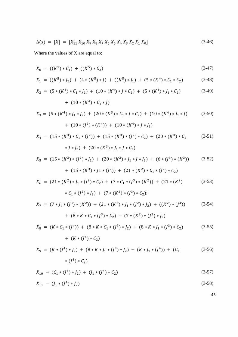
∆(𝑠) = [𝑋] = [𝑋11 𝑋10 𝑋9 𝑋8 𝑋7 𝑋6 𝑋5 𝑋4 𝑋3 𝑋2 𝑋1 𝑋0] (3-46)

Where the values of X are equal to:

𝑋0 = ((𝐾5) ∗ 𝐶1) + ((𝐾5) ∗ 𝐶2) (3-47)

𝑋1 = ((𝐾5) ∗ 𝐽2) + (4 ∗ (𝐾5) ∗ 𝐽) + ((𝐾5) ∗ 𝐽1) + (5 ∗ (𝐾4) ∗ 𝐶1 ∗ 𝐶2) (3-48)

𝑋2 = (5 ∗ (𝐾4) ∗ 𝐶1 ∗ 𝐽2) + (10 ∗ (𝐾4) ∗ 𝐽 ∗ 𝐶2) + (5 ∗ (𝐾4) ∗ 𝐽1 ∗ 𝐶2)

+ (10 ∗ (𝐾4) ∗ 𝐶1 ∗ 𝐽)

(3-49)

𝑋3 = (5 ∗ (𝐾4) ∗ 𝐽1 ∗ 𝐽2) + (20 ∗ (𝐾3) ∗ 𝐶1 ∗ 𝐽 ∗ 𝐶2) + (10 ∗ (𝐾4) ∗ 𝐽1 ∗ 𝐽)

+ (10 ∗ (𝐽2) ∗ (𝐾4)) + (10 ∗ (𝐾4) ∗ 𝐽 ∗ 𝐽2)

(3-50)

𝑋4 = (15 ∗ (𝐾3) ∗ 𝐶1 ∗ (𝐽2)) + (15 ∗ (𝐾3) ∗ (𝐽2) ∗ 𝐶2) + (20 ∗ (𝐾3) ∗ 𝐶1

∗ 𝐽 ∗ 𝐽2) + (20 ∗ (𝐾3) ∗ 𝐽1 ∗ 𝐽 ∗ 𝐶2)

(3-51)

𝑋5 = (15 ∗ (𝐾3) ∗ (𝐽2) ∗ 𝐽2) + (20 ∗ (𝐾3) ∗ 𝐽1 ∗ 𝐽 ∗ 𝐽2) + (6 ∗ (𝐽3) ∗ (𝐾3))

+ (15 ∗ (𝐾3) ∗ 𝐽1 ∗ (𝐽2)) + (21 ∗ (𝐾2) ∗ 𝐶1 ∗ (𝐽2) ∗ 𝐶2)

(3-52)

𝑋6 = (21 ∗ (𝐾2) ∗ 𝐽1 ∗ (𝐽2) ∗ 𝐶2) + (7 ∗ 𝐶1 ∗ (𝐽3) ∗ (𝐾2)) + (21 ∗ (𝐾2)

∗ 𝐶1 ∗ (𝐽2) ∗ 𝐽2) + (7 ∗ (𝐾2) ∗ (𝐽3) ∗ 𝐶2);

(3-53)

𝑋7 = (7 ∗ 𝐽1 ∗ (𝐽3) ∗ (𝐾2)) + (21 ∗ (𝐾2) ∗ 𝐽1 ∗ (𝐽2) ∗ 𝐽2) + ((𝐾2) ∗ (𝐽4))

+ (8 ∗ 𝐾 ∗ 𝐶1 ∗ (𝐽3) ∗ 𝐶2) + (7 ∗ (𝐾2) ∗ (𝐽3) ∗ 𝐽2)

(3-54)

𝑋8 = (𝐾 ∗ 𝐶1 ∗ (𝐽4)) + (8 ∗ 𝐾 ∗ 𝐶1 ∗ (𝐽3) ∗ 𝐽2) + (8 ∗ 𝐾 ∗ 𝐽1 ∗ (𝐽3) ∗ 𝐶2)

+ (𝐾 ∗ (𝐽4) ∗ 𝐶2)

(3-55)

𝑋9 = (𝐾 ∗ (𝐽4) ∗ 𝐽2) + (8 ∗ 𝐾 ∗ 𝐽1 ∗ (𝐽3) ∗ 𝐽2) + (𝐾 ∗ 𝐽1 ∗ (𝐽4)) + (𝐶1

∗ (𝐽4) ∗ 𝐶2)

(3-56)

𝑋10 = (𝐶1 ∗ (𝐽4) ∗ 𝐽2) + (𝐽1 ∗ (𝐽4) ∗ 𝐶2) (3-57)

𝑋11 = (𝐽1 ∗ (𝐽4) ∗ 𝐽2) (3-58)

44

This answer is already divided by S since 𝑊 (𝑠) = 𝑠 ∗ 𝜃(𝑠)

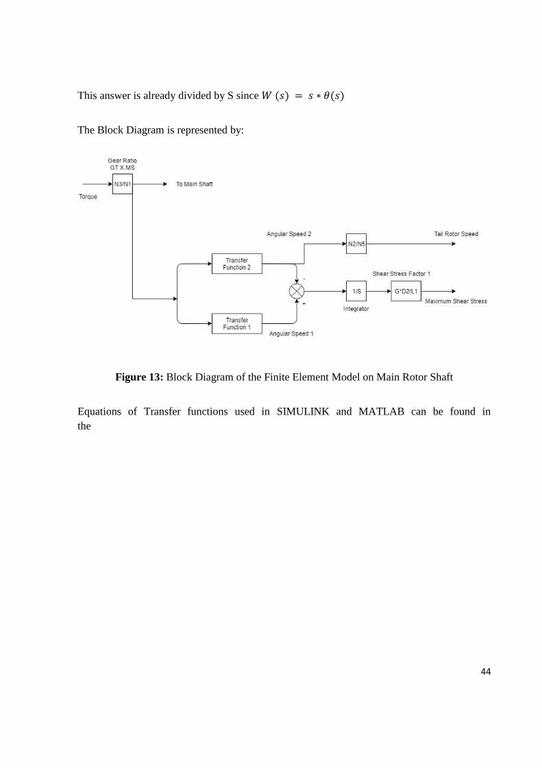
The Block Diagram is represented by:

Figure 13: Block Diagram of the Finite Element Model on Main Rotor Shaft


the

45

Appendix I.

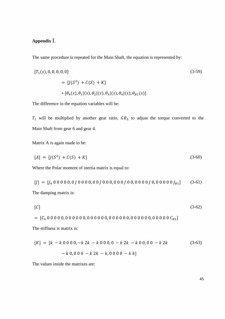
The same procedure is repeated for the Main Shaft, the equation is represented by:

[𝑇1(𝑠), 0, 0, 0, 0, 0]

= [𝐽(𝑆2) + 𝐶(𝑆) + 𝐾]

∗ [𝜃4(𝑠), 𝜃1|(𝑠), 𝜃2|(𝑠), 𝜃3|(𝑠), 𝜃4|(𝑠), 𝜃𝐵1(𝑠)]

(3-59)

The difference in the equation variables will be:

𝑇1 will be multiplied by another gear ratio, 𝐺𝑅3 to adjust the torque converted to the

Main Shaft from gear 6 and gear 4.

Matrix A is again made to be:

[𝐴] = [𝐽(𝑆2) + 𝐶(𝑆) + 𝐾] (3-60)

Where the Polar moment of inertia matrix is equal to:

[𝐽] = [𝐽4 0 0 0 0 0, 0 𝐽 0 0 0 0, 0 0 𝐽 0 0 0, 0 0 0 𝐽 0 0, 0 0 0 0 𝐽 0, 0 0 0 0 0 𝐽𝐵1] (3-61)

The damping matrix is:

[𝐶]

= [𝐶4 0 0 0 0 0, 0 0 0 0 0 0, 0 0 0 0 0 0, 0 0 0 0 0 0, 0 0 0 0 0 0, 0 0 0 0 0 𝐶𝐵1]

(3-62)

The stiffness is matrix is:

[𝐾] = [𝑘 − 𝑘 0 0 0 0, −𝑘 2𝑘 − 𝑘 0 0 0, 0 − 𝑘 2𝑘 − 𝑘 0 0, 0 0 − 𝑘 2𝑘

− 𝑘 0, 0 0 0 − 𝑘 2𝑘 − 𝑘, 0 0 0 0 − 𝑘 𝑘]

(3-63)

The values inside the matrixes are:

46

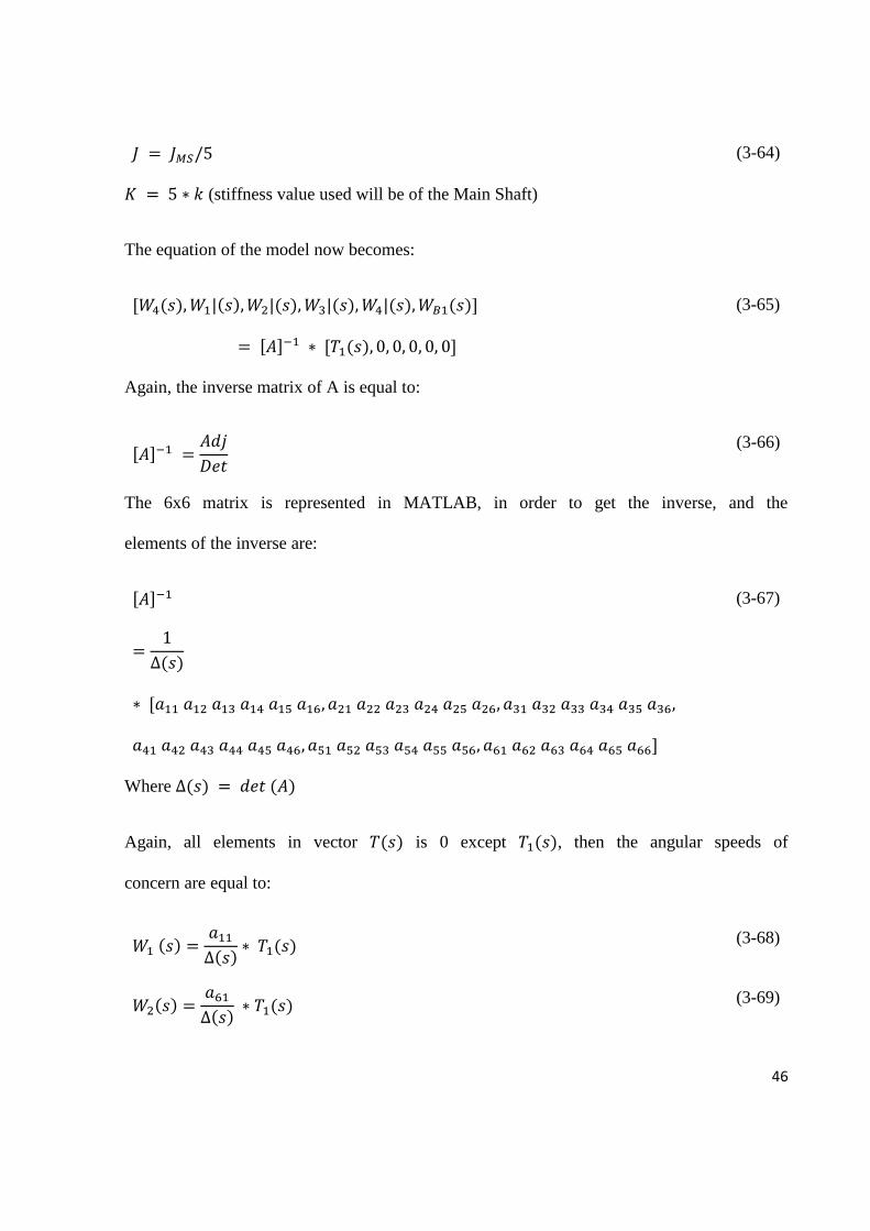
𝐽 = 𝐽𝑀𝑆/5 (3-64)

𝐾 = 5 ∗ 𝑘 (stiffness value used will be of the Main Shaft)

The equation of the model now becomes:

[𝑊4(𝑠), 𝑊1|(𝑠), 𝑊2|(𝑠), 𝑊3|(𝑠), 𝑊4|(𝑠), 𝑊𝐵1(𝑠)]

= [𝐴]−1 ∗ [𝑇1(𝑠), 0, 0, 0, 0, 0]

(3-65)

Again, the inverse matrix of A is equal to:

[𝐴]−1 =𝐴𝑑𝑗

𝐷𝑒𝑡

(3-66)

The 6x6 matrix is represented in MATLAB, in order to get the inverse, and the

elements of the inverse are:

[𝐴]−1

=1

∆(𝑠)

∗ [𝑎11 𝑎12 𝑎13 𝑎14 𝑎15 𝑎16, 𝑎21 𝑎22 𝑎23 𝑎24 𝑎25 𝑎26, 𝑎31 𝑎32 𝑎33 𝑎34 𝑎35 𝑎36,

𝑎41 𝑎42 𝑎43 𝑎44 𝑎45 𝑎46, 𝑎51 𝑎52 𝑎53 𝑎54 𝑎55 𝑎56, 𝑎61 𝑎62 𝑎63 𝑎64 𝑎65 𝑎66]

(3-67)

Where ∆(𝑠) = 𝑑𝑒𝑡 (𝐴)

Again, all elements in vector 𝑇(𝑠) is 0 except 𝑇1(𝑠), then the angular speeds of

concern are equal to:

𝑊1 (𝑠) =𝑎11

∆(𝑠)∗ 𝑇1(𝑠) (3-68)

𝑊2(𝑠) =𝑎61

∆(𝑠) ∗ 𝑇1(𝑠) (3-69)

47

𝐴11 = 𝐽𝑀𝑆4 ∗ 𝐾 ∗ 𝑆8 + 𝐽𝐵1 ∗ 𝐽𝑀𝑆

4 ∗ 𝑆10 + 𝐶𝐵1 ∗ 𝐽𝑀𝑆4 ∗ 𝑆9 + 35 ∗ 𝐽𝑀𝑆

3 ∗ 𝐾2

∗ 𝑆6 + 40 ∗ 𝐽𝐵1 ∗ 𝐽𝑀𝑆3 ∗ 𝐾 ∗ 𝑆8 + 40 ∗ 𝐶𝐵1 ∗ 𝐽𝑀𝑆

3 ∗ 𝐾 ∗ 𝑆7

+ 375 ∗ 𝐽𝑀𝑆2 ∗ 𝐾3 ∗ 𝑆4 + 525 ∗ 𝐽𝐵1 ∗ 𝐽𝑀𝑆

2 ∗ 𝐾2 ∗ 𝑆6 + 525

∗ 𝐶𝐵1 ∗ 𝐽𝑀𝑆2 ∗ 𝐾2 ∗ 𝑆5 + 1250 ∗ 𝐽𝑀𝑆 ∗ 𝐾4 ∗ 𝑆2 + 2500 ∗ 𝐽𝐵1

∗ 𝐽𝑀𝑆 ∗ 𝐾3 ∗ 𝑆4 + 2500 ∗ 𝐶𝐵1 ∗ 𝐽𝑀𝑆 ∗ 𝐾3 ∗ 𝑆3 + 625 ∗ 𝐾5

+ 3125 ∗ 𝐽𝐵1 ∗ 𝐾4 ∗ 𝑆2 + 3125 ∗ 𝐶𝐵1 ∗ 𝐾4 ∗ 𝑆

(3-70)

𝐴61 = 𝐾5 (3-71)

The values can be represented in a more proper fashion and rearranged as of

descending powers of S, in MATLAB this is done by writing it in form of a matrix

[W]

𝐴11 = [𝑊] = [𝑊10 𝑊9 𝑊8 𝑊7 𝑊6 𝑊5 𝑊4 𝑊3 𝑊2 𝑊1 𝑊0] (3-72)

Where the values of W are:

𝑊0 = (𝐾5) (3-73)

𝑊1 = (5 ∗ (𝐾4) ∗ 𝐶𝐵1) (3-74)

𝑊2 = (5 ∗ (𝐾4) ∗ 𝐽𝐵1) + (10 ∗ (𝐾4) ∗ 𝐽) (3-75)

𝑊3 = (20 ∗ (𝐾3) ∗ 𝐽 ∗ 𝐶𝐵1) (3-76)

𝑊4 = (15 ∗ (𝐾3) ∗ (𝐽2)) + (20 ∗ (𝐾3) ∗ 𝐽 ∗ 𝐽𝐵1) (3-77)

𝑊5 = (21 ∗ (𝐾2) ∗ (𝐽2) ∗ 𝐶𝐵1) (3-78)

𝑊6 = (7 ∗ (𝐽3) ∗ (𝐾2)) + (21 ∗ (𝐾2) ∗ (𝐽2) ∗ 𝐽𝐵1) (3-79)

𝑊7 = (8 ∗ 𝐾 ∗ (𝐽3) ∗ 𝐶𝐵1) (3-80)

𝑊8 = (8 ∗ 𝐾 ∗ (𝐽3) ∗ 𝐽𝐵1) + (𝐾 ∗ (𝐽4)) (3-81)

48

𝑊9 = ((𝐽4) ∗ 𝐶𝐵1) (3-82)

𝑊10 = ((𝐽4) ∗ 𝐽𝐵1) (3-83)

𝐴61 = [𝑊0] (3-84)

∆(𝑠) is also found to be:

49

∆(𝑠) = 625 ∗ 𝐽4 ∗ 𝐾5 ∗ 𝑆2 + 500 ∗ 𝐽𝑀𝑆 ∗ 𝐾5 ∗ 𝑆2 + 625 ∗ 𝐽𝐵1 ∗ 𝐾5 ∗ 𝑆2

+ 250 ∗ 𝐽𝑀𝑆2 ∗ 𝐾4 ∗ 𝑆4 + 30 ∗ 𝐽𝑀𝑆

3 ∗ 𝐾3 ∗ 𝑆6 + 𝐽𝑀𝑆4 ∗ 𝐾2 ∗ 𝑆8

+ 625 ∗ 𝐶4 ∗ 𝐾5 ∗ 𝑆 + 625 ∗ 𝐶𝐵1 ∗ 𝐾5 ∗ 𝑆 + 𝐶4 ∗ 𝐶𝐵1 ∗ 𝐽𝑀𝑆4

∗ 𝑆10 + 3125 ∗ 𝐶4 ∗ 𝐶𝐵1 ∗ 𝐾4 ∗ 𝑆2 + 𝐶4 ∗ 𝐽𝑀𝑆4 ∗ 𝐽𝐵1 ∗ 𝑆11

+ 𝐶𝐵1 ∗ 𝐽4 ∗ 𝐽𝑀𝑆4 ∗ 𝑆11 + 1250 ∗ 𝐶4 ∗ 𝐽𝑀𝑆 ∗ 𝐾4 ∗ 𝑆3 + 𝐶4 ∗ 𝐽𝑀𝑆

4

∗ 𝐾 ∗ 𝑆9 + 3125 ∗ 𝐶4 ∗ 𝐽𝐵1 ∗ 𝐾4 ∗ 𝑆3 + 3125 ∗ 𝐶𝐵1 ∗ 𝐽4 ∗ 𝐾4

∗ 𝑆3 + 1250 ∗ 𝐶𝐵1 ∗ 𝐽𝑀𝑆 ∗ 𝐾4 ∗ 𝑆3 + 𝐶𝐵1 ∗ 𝐽𝑀𝑆4 ∗ 𝐾 ∗ 𝑆9 + 𝐽4

∗ 𝐽𝑀𝑆4 ∗ 𝐽𝐵1 ∗ 𝑆12 + 1250 ∗ 𝐽4 ∗ 𝐽𝑀𝑆 ∗ 𝐾4 ∗ 𝑆4 + 𝐽4 ∗ 𝐽𝑀𝑆

4 ∗ 𝐾

∗ 𝑆10 + 3125 ∗ 𝐽4 ∗ 𝐽𝐵1 ∗ 𝐾4 ∗ 𝑆4 + 1250 ∗ 𝐽𝑀𝑆 ∗ 𝐽𝐵1 ∗ 𝐾4

∗ 𝑆4 + 𝐽𝑀𝑆4 ∗ 𝐽𝐵1 ∗ 𝐾 ∗ 𝑆10 + 375 ∗ 𝐶4 ∗ 𝐽𝑀𝑆

2 ∗ 𝐾3 ∗ 𝑆5 + 35

∗ 𝐶4 ∗ 𝐽𝑀𝑆3 ∗ 𝐾2 ∗ 𝑆7 + 375 ∗ 𝐶𝐵1 ∗ 𝐽𝑀𝑆

2 ∗ 𝐾3 ∗ 𝑆5 + 35 ∗ 𝐶𝐵1

∗ 𝐽𝑀𝑆3 ∗ 𝐾2 ∗ 𝑆7 + 375 ∗ 𝐽4 ∗ 𝐽𝑀𝑆

2 ∗ 𝐾3 ∗ 𝑆6 + 35 ∗ 𝐽4 ∗ 𝐽𝑀𝑆3

∗ 𝐾2 ∗ 𝑆8 + 375 ∗ 𝐽𝑀𝑆2 ∗ 𝐽𝐵1 ∗ 𝐾3 ∗ 𝑆6 + 35 ∗ 𝐽𝑀𝑆

3 ∗ 𝐽𝐵1 ∗ 𝐾2

∗ 𝑆8 + 2500 ∗ 𝐶4 ∗ 𝐶𝐵1 ∗ 𝐽𝑀𝑆 ∗ 𝐾3 ∗ 𝑆4 + 40 ∗ 𝐶4 ∗ 𝐶𝐵1 ∗ 𝐽𝑀𝑆3

∗ 𝐾 ∗ 𝑆8 + 2500 ∗ 𝐶4 ∗ 𝐽𝑀𝑆 ∗ 𝐽𝐵1 ∗ 𝐾3 ∗ 𝑆5 + 2500 ∗ 𝐶𝐵1 ∗ 𝐽4

∗ 𝐽𝑀𝑆 ∗ 𝐾3 ∗ 𝑆5 + 40 ∗ 𝐶4 ∗ 𝐽𝑀𝑆3 ∗ 𝐽𝐵1 ∗ 𝐾 ∗ 𝑆9 + 40 ∗ 𝐶𝐵1 ∗ 𝐽4

∗ 𝐽𝑀𝑆3 ∗ 𝐾 ∗ 𝑆9 + 2500 ∗ 𝐽4 ∗ 𝐽𝑀𝑆 ∗ 𝐽𝐵1 ∗ 𝐾3 ∗ 𝑆6 + 40 ∗ 𝐽4

∗ 𝐽𝑀𝑆3 ∗ 𝐽𝐵1 ∗ 𝐾 ∗ 𝑆10 + 525 ∗ 𝐶4 ∗ 𝐶𝐵1 ∗ 𝐽𝑀𝑆

2 ∗ 𝐾2 ∗ 𝑆6 + 525

∗ 𝐶4 ∗ 𝐽𝑀𝑆2 ∗ 𝐽𝐵1 ∗ 𝐾2 ∗ 𝑆7 + 525 ∗ 𝐶𝐵1 ∗ 𝐽4 ∗ 𝐽𝑀𝑆

2 ∗ 𝐾2 ∗ 𝑆7

+ 525 ∗ 𝐽4 ∗ 𝐽𝑀𝑆2 ∗ 𝐽𝐵1 ∗ 𝐾2 ∗ 𝑆8

(3-85)

∆(𝑠) is also represented by a matrix in MATLAB, the matrix of [V]:

∆(𝑠) = [𝑉] = [𝑉11 𝑉10 𝑉9 𝑉8 𝑉7 𝑉6 𝑉5 𝑉4 𝑉3 𝑉2 𝑉1 𝑉0] (3-86)

50

Where the values of matrix V are:

𝑉0 = ((𝐾5) ∗ 𝐶4) + ((𝐾5) ∗ 𝐶𝐵1) (3-87)

𝑉1 = ((𝐾5) ∗ 𝐽𝐵1) + (4 ∗ (𝐾5) ∗ 𝐽) + ((𝐾5) ∗ 𝐽4) + (5 ∗ (𝐾4) ∗ 𝐶4 ∗ 𝐶𝐵1) (3-88)

𝑉2 = (5 ∗ (𝐾4) ∗ 𝐶4 ∗ 𝐽𝐵1) + (10 ∗ (𝐾4) ∗ 𝐽 ∗ 𝐶𝐵1) + (5 ∗ (𝐾4) ∗ 𝐽4 ∗ 𝐶𝐵1)

+ (10 ∗ (𝐾4) ∗ 𝐶4 ∗ 𝐽)

(3-89)

𝑉3 = (5 ∗ (𝐾4) ∗ 𝐽4 ∗ 𝐽𝐵1) + (20 ∗ (𝐾3) ∗ 𝐶4 ∗ 𝐽 ∗ 𝐶𝐵1) + (10 ∗ (𝐾4) ∗ 𝐽4

∗ 𝐽) + (10 ∗ (𝐽2) ∗ (𝐾4)) + (10 ∗ (𝐾4) ∗ 𝐽 ∗ 𝐽𝐵1)

(3-90)

𝑉4 = (15 ∗ (𝐾3) ∗ 𝐶4 ∗ (𝐽2)) + (15 ∗ (𝐾3) ∗ (𝐽2) ∗ 𝐶𝐵1) + (20 ∗ (𝐾3) ∗ 𝐶4

∗ 𝐽 ∗ 𝐽𝐵1) + (20 ∗ (𝐾3) ∗ 𝐽4 ∗ 𝐽 ∗ 𝐶𝐵1)

(3-91)

𝑉5 = (15 ∗ (𝐾3) ∗ (𝐽2) ∗ 𝐽𝐵1) + (20 ∗ (𝐾3) ∗ 𝐽4 ∗ 𝐽 ∗ 𝐽𝐵1) + (6 ∗ (𝐽3)

∗ (𝐾3)) + (15 ∗ (𝐾3) ∗ 𝐽4 ∗ (𝐽2)) + (21 ∗ (𝐾2) ∗ 𝐶4 ∗ (𝐽2)

∗ 𝐶𝐵1)

(3-92)

𝑉6 = (21 ∗ (𝐾2) ∗ 𝐽4 ∗ (𝐽2) ∗ 𝐶𝐵1) + (7 ∗ 𝐶4 ∗ (𝐽3) ∗ (𝐾2)) + (21 ∗ (𝐾2)

∗ 𝐶4 ∗ (𝐽2) ∗ 𝐽𝐵1) + (7 ∗ (𝐾2) ∗ (𝐽3) ∗ 𝐶𝐵1)

(3-93)

𝑉7 = (7 ∗ 𝐽4 ∗ (𝐽3) ∗ (𝐾2)) + (21 ∗ (𝐾2) ∗ 𝐽4 ∗ (𝐽2) ∗ 𝐽𝐵1) + ((𝐾2) ∗ (𝐽4))

+ (8 ∗ 𝐾 ∗ 𝐶4 ∗ (𝐽3) ∗ 𝐶𝐵1) + (7 ∗ (𝐾2) ∗ (𝐽3) ∗ 𝐽𝐵1)

(3-94)

𝑉8 = (𝐾 ∗ 𝐶4 ∗ (𝐽4)) + (8 ∗ 𝐾 ∗ 𝐶4 ∗ (𝐽3) ∗ 𝐽𝐵1) + (8 ∗ 𝐾 ∗ 𝐽4 ∗ (𝐽3) ∗ 𝐶𝐵1)

+ (𝐾 ∗ (𝐽4) ∗ 𝐶𝐵1)

(3-95)

𝑉9 = (𝐾 ∗ (𝐽4) ∗ 𝐽𝐵1) + (8 ∗ 𝐾 ∗ 𝐽4 ∗ (𝐽3) ∗ 𝐽𝐵1) + (𝐾 ∗ 𝐽4 ∗ (𝐽4)) + (𝐶4

∗ (𝐽4) ∗ 𝐶𝐵1)

(3-96)

𝑉10 = (𝐶4 ∗ (𝐽4) ∗ 𝐽𝐵1) + (𝐽4 ∗ (𝐽4) ∗ 𝐶𝐵1) (3-97)

𝑉11 = (𝐽4 ∗ (𝐽4) ∗ 𝐽𝐵1) (3-98)

51

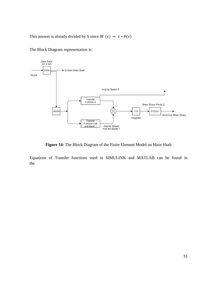
This answer is already divided by S since 𝑊 (𝑠) = 𝑠 ∗ 𝜃(𝑠)

The Block Diagram representation is:

Figure 14: The Block Diagram of the Finite Element Model on Main Shaft


the

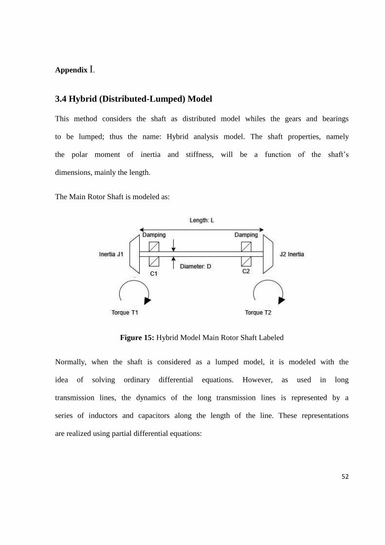
52

Appendix I.

3.4 Hybrid (Distributed-Lumped) Model

This method considers the shaft as distributed model whiles the gears and bearings

to be lumped; thus the name: Hybrid analysis model. The shaft properties, namely

the polar moment of inertia and stiffness, will be a function of the shaft’s

dimensions, mainly the length.

The Main Rotor Shaft is modeled as:

Figure 15: Hybrid Model Main Rotor Shaft Labeled

Normally, when the shaft is considered as a lumped model, it is modeled with the

idea of solving ordinary differential equations. However, as used in long

transmission lines, the dynamics of the long transmission lines is represented by a

series of inductors and capacitors along the length of the line. These representations

are realized using partial differential equations:

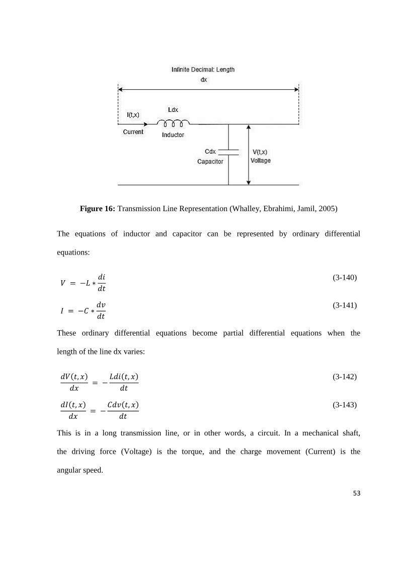
53

Figure 16: Transmission Line Representation (Whalley, Ebrahimi, Jamil, 2005)

The equations of inductor and capacitor can be represented by ordinary differential

equations:

𝑉 = −𝐿 ∗𝑑𝑖

𝑑𝑡

(3-140)

𝐼 = −𝐶 ∗𝑑𝑣

𝑑𝑡

(3-141)

These ordinary differential equations become partial differential equations when the

length of the line dx varies:

𝑑𝑉(𝑡, 𝑥)

𝑑𝑥 = −

𝐿𝑑𝑖(𝑡, 𝑥)

𝑑𝑡

(3-142)

𝑑𝐼(𝑡, 𝑥)

𝑑𝑥 = −

𝐶𝑑𝑣(𝑡, 𝑥)

𝑑𝑡

(3-143)

This is in a long transmission line, or in other words, a circuit. In a mechanical shaft,

the driving force (Voltage) is the torque, and the charge movement (Current) is the

angular speed.

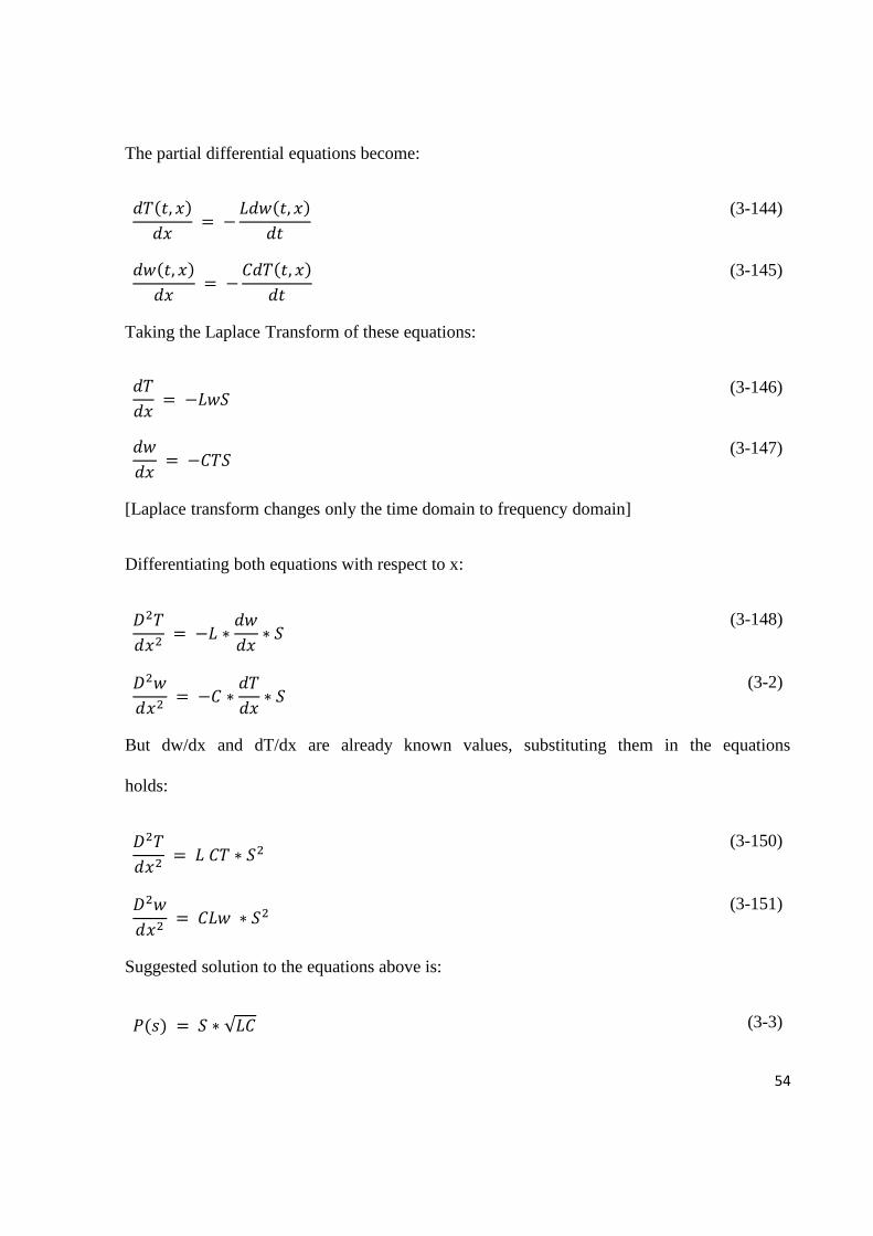
54

The partial differential equations become:

𝑑𝑇(𝑡, 𝑥)

𝑑𝑥 = −

𝐿𝑑𝑤(𝑡, 𝑥)

𝑑𝑡

(3-144)

𝑑𝑤(𝑡, 𝑥)

𝑑𝑥 = −

𝐶𝑑𝑇(𝑡, 𝑥)

𝑑𝑡

(3-145)

Taking the Laplace Transform of these equations:

𝑑𝑇

𝑑𝑥 = −𝐿𝑤𝑆

(3-146)

𝑑𝑤

𝑑𝑥 = −𝐶𝑇𝑆

(3-147)

[Laplace transform changes only the time domain to frequency domain]

Differentiating both equations with respect to x:

𝐷2𝑇

𝑑𝑥2 = −𝐿 ∗

𝑑𝑤

𝑑𝑥∗ 𝑆

(3-148)

𝐷2𝑤

𝑑𝑥2 = −𝐶 ∗

𝑑𝑇

𝑑𝑥∗ 𝑆

(3-2)

But dw/dx and dT/dx are already known values, substituting them in the equations

holds:

𝐷2𝑇

𝑑𝑥2 = 𝐿 𝐶𝑇 ∗ 𝑆2

(3-150)

𝐷2𝑤

𝑑𝑥2 = 𝐶𝐿𝑤 ∗ 𝑆2

(3-151)

Suggested solution to the equations above is:

𝑃(𝑠) = 𝑆 ∗ √𝐿𝐶 (3-3)

55

This would be called: the propagation function

Applying the propagation function to the partial differential equations; the general

solution becomes:

𝑇 = 𝑃1 ∗ 𝐶𝑜𝑠ℎ[𝑃(𝑠)𝑥] + 𝑃2 ∗ 𝑆𝑖𝑛ℎ[𝑃(𝑠)𝑥] (3-4)

𝑊 = 𝑃3 ∗ 𝑆𝑖𝑛ℎ[𝑃(𝑠)𝑥] + 𝑃4 ∗ 𝐶𝑜𝑠ℎ[𝑃(𝑠)𝑥] (3-53)

To find the constants, 𝑃1 𝑃2 𝑃3 𝑃4, initial conditions have to be satisfied.

Using the properties of hyperbolic functions:

𝑆𝑖𝑛ℎ(0) = 0 (3-154)

𝐶𝑜𝑠ℎ(0) = 1 (3-155)

Initial condition x = 0

𝑇(𝑠 = 𝑠, 𝑥 = 0) = 𝑃1 (3-156)

𝑊(𝑠 = 𝑠, 𝑥 = 0) = 𝑃4 (3-157)

Differentiating the general solutions:

𝑑𝑇

𝑑𝑥 = 𝑃1 ∗ 𝑃(𝑠) ∗ 𝑆𝑖𝑛ℎ[𝑃(𝑠)𝑥] + 𝑃2 ∗ 𝑃(𝑠) ∗ 𝐶𝑜𝑠ℎ[𝑃(𝑠)𝑥]

(3-158)

𝑑𝑊

𝑑𝑥 = 𝑃3 ∗ 𝑃(𝑠) ∗ 𝐶𝑜𝑠ℎ[𝑃(𝑠)𝑥] + 𝑃4 ∗ 𝑃(𝑠) ∗ 𝑆𝑖𝑛ℎ[𝑃(𝑠)𝑥]

(3-159)

But also:

𝑑𝑇

𝑑𝑥 = −𝐿𝑤𝑆

(3-160)

𝑑𝑤

𝑑𝑥 = −𝐶𝑇𝑆

(3-161)

56

Equating both equations:

−𝐿𝑤𝑆 = 𝑃1 ∗ 𝑃(𝑠) ∗ 𝑆𝑖𝑛ℎ[𝑃(𝑠)𝑥] + 𝑃2 ∗ 𝑃(𝑠) ∗ 𝐶𝑜𝑠ℎ[𝑃(𝑠)𝑥] (3-162)

−𝐶𝑇𝑆 = 𝑃3 ∗ 𝑃(𝑠) ∗ 𝐶𝑜𝑠ℎ[𝑃(𝑠)𝑥] + 𝑃4 ∗ 𝑃(𝑠) ∗ 𝑆𝑖𝑛ℎ[𝑃(𝑠)𝑥] (3-4-163)

Initial condition at x= 0:

−𝐿𝑤𝑆 = 𝑃2 ∗ 𝑃(𝑠) (3-164)

−𝐶𝑇𝑆 = 𝑃3 ∗ 𝑃(𝑠) (3-165)

𝑃2 = −𝐿 ∗ 𝑤 ∗𝑆

𝑃(𝑠)

(3-165)

𝑃3 = −𝐶 ∗ 𝑇 ∗𝑆

𝑃(𝑠)

(3-166)

Where 𝑤 is 𝑤(𝑠 = 𝑠, 𝑥 = 0) and 𝑇 is 𝑇(𝑠 = 𝑠, 𝑥 = 0)

Since 𝑃(𝑠) = 𝑆 ∗ √𝐿𝐶

𝑃2 = −𝐿 ∗ 𝑤(𝑠 = 𝑠, 𝑥 = 0) ∗𝑆

𝑆∗ √(𝐿𝐶)

(3-167)

𝑃2 = −√𝐿

𝐶∗ 𝑤(𝑠 = 𝑠, 𝑥 = 0)

(3-168)

𝑃3 = −𝐶 ∗ 𝑇(𝑠 = 𝑙𝑠, 𝑥 = 0) ∗𝑆

𝑆∗ √𝐿𝐶

(3-169)

𝑃3 = −√𝐶

𝐿∗ 𝑇(𝑠 = 𝑠, 𝑥 = 0)

(3-170)

The term √𝐿

𝐶 is defined as the impedance:

57

𝜁 = √𝐿

𝐶

(3-171)

1

𝜁 = √

𝐶

𝐿

(3-172)

This defines 𝑃2 and 𝑃3 to be:

𝑃2 = −√𝐿

𝐶∗ 𝑤(𝑠 = 𝑠, 𝑥 = 0)

(3-173)

𝑃2 = − 𝜁 ∗ 𝑤(𝑠 = 𝑠, 𝑥 = 0) (3-174)

𝑃3 = −√𝐶

𝐿∗ 𝑇(𝑠 = 𝑠, 𝑥 = 0)

(3-175)

𝑃3 = −(1

𝜁) ∗ 𝑇(𝑠 = 𝑠, 𝑥 = 0)

(3-176)

The general solution for the partial differential equations becomes:

𝑇 = 𝑇(𝑠 = 𝑠, 𝑥 = 0) ∗ 𝐶𝑜𝑠ℎ[𝑃(𝑠)𝑥] − 𝜁 ∗ 𝑤(𝑠 = 𝑠, 𝑥 = 0) ∗ 𝑆𝑖𝑛ℎ[𝑃(𝑠)𝑥] (3-177)

𝑊 = − (1

𝜁) ∗ 𝑇(𝑠 = 𝑠, 𝑥 = 0) ∗ 𝑆𝑖𝑛ℎ[𝑃(𝑠)𝑥] + 𝑊(𝑠 = 𝑠, 𝑥

= 0) ∗ 𝐶𝑜𝑠ℎ[𝑃(𝑠)𝑥]

(3-178)

To write the equation in matrix form:

[𝑇] = [𝐴] ∗ [𝑊] (3-179)

From 𝑊:

58

𝑊 = − (1

𝜁) ∗ 𝑇(𝑠 = 𝑠, 𝑥 = 0) ∗ 𝑆𝑖𝑛ℎ[𝑃(𝑠)𝑥] + 𝑊(𝑠 = 𝑠, 𝑥

= 0) ∗ 𝐶𝑜𝑠ℎ[𝑃(𝑠)𝑥]

(3-180)

𝑇(𝑠 = 𝑠, 𝑥 = 0) = − 𝜁 ∗ (1

𝑆𝑖𝑛ℎ[𝑃(𝑠)𝑥]) ∗ 𝑊 + 𝜁 ∗ 𝐶𝑜𝑡ℎ[𝑃(𝑠)𝑥] ∗ 𝑊(𝑠

= 𝑠, 𝑥 = 0)

(3-181)

𝐶𝑜𝑠𝑒𝑐ℎ[𝑃(𝑠)𝑥] = 1/𝑆𝑖𝑛ℎ[𝑃(𝑠)𝑥] (3-182)

𝑇(𝑠 = 𝑠, 𝑥 = 0) = − 𝜁 ∗ 𝐶𝑜𝑠𝑒𝑐ℎ[𝑃(𝑠)𝑥] ∗ 𝑊 + 𝜁 ∗ 𝐶𝑜𝑡ℎ[𝑃(𝑠)𝑥] ∗ 𝑊(𝑠

= 𝑠, 𝑥 = 0)

(3-183)

Substituting the acquired equation into 𝑇:

𝑇 = [− 𝜁 ∗ 𝐶𝑜𝑠𝑒𝑐ℎ[𝑃(𝑠)𝑥] ∗ 𝑊 + 𝜁 ∗ 𝐶𝑜𝑡ℎ[𝑃(𝑠)𝑥] ∗ 𝑊(𝑠 = 𝑠, 𝑥

= 0)] ∗ 𝐶𝑜𝑠ℎ[𝑃(𝑠)𝑥] − 𝜁 ∗ 𝑤(𝑠 = 𝑠, 𝑥 = 0) ∗ 𝑆𝑖𝑛ℎ[𝑃(𝑠)𝑥]

(3-184)

Where:

𝐶𝑜𝑠𝑒𝑐ℎ ∗ 𝐶𝑜𝑠ℎ = 𝐶𝑜𝑡ℎ (3-185)

𝐶𝑜𝑡ℎ ∗ 𝐶𝑜𝑠ℎ =𝐶𝑜𝑠ℎ2

𝑆𝑖𝑛ℎ

(3-186)

(𝐶𝑜𝑠ℎ2

𝑆𝑖𝑛ℎ) – 𝑆𝑖𝑛ℎ =

𝐶𝑜𝑠ℎ2 – 𝑆𝑖𝑛ℎ2

𝑆𝑖𝑛ℎ =

1

𝑆𝑖𝑛ℎ = 𝐶𝑜𝑠𝑒𝑐ℎ

(3-187)

This implies that:

𝑇 = −𝜁 ∗ 𝐶𝑜𝑙𝑡ℎ[𝑃(𝑠)𝑥] ∗ 𝑊 + 𝜁 ∗ 𝑊(𝑠 = 𝑠, 𝑥 = 0) ∗ 𝐶𝑜𝑠𝑒𝑐ℎ[𝑃(𝑠)𝑥] (3-188)

Taking both equations of 𝑇 and 𝑇(𝑠 = 𝑠, 𝑥 = 0), putting them in matrix form:

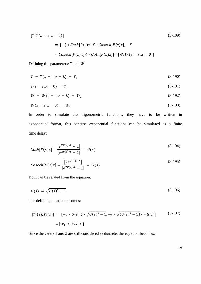
59

[𝑇, 𝑇(𝑠 = 𝑠, 𝑥 = 0)]

= [−𝜁 ∗ 𝐶𝑜𝑡ℎ[𝑃(𝑠)𝑥] 𝜁 ∗ 𝐶𝑜𝑠𝑒𝑐ℎ[𝑃(𝑠)𝑥], − 𝜁

∗ 𝐶𝑜𝑠𝑒𝑐ℎ[𝑃(𝑠)𝑥] 𝜁 ∗ 𝐶𝑜𝑡ℎ[𝑃(𝑠)𝑥]] ∗ [𝑊, 𝑊(𝑠 = 𝑠, 𝑥 = 0)]

(3-189)

Defining the parameters: 𝑇 and 𝑊

𝑇 = 𝑇(𝑠 = 𝑠, 𝑥 = 𝐿) = 𝑇2 (3-190)

𝑇(𝑠 = 𝑠, 𝑥 = 0) = 𝑇1 (3-191)

𝑊 = 𝑊(𝑠 = 𝑠, 𝑥 = 𝐿) = 𝑊2 (3-192)

𝑊(𝑠 = 𝑠, 𝑥 = 0) = 𝑊1 (3-193)

In order to simulate the trigonometric functions, they have to be written in

exponential format, this because exponential functions can be simulated as a finite

time delay:

𝐶𝑜𝑡ℎ[𝑃(𝑠)𝑥] =[𝑒2𝑃(𝑠)∗𝐿 + 1]

[𝑒2𝑃(𝑠)∗𝐿 − 1] = 𝐺(𝑠)

(3-194)

𝐶𝑜𝑠𝑒𝑐ℎ[𝑃(𝑠)𝑥] =[2𝑒2𝑃(𝑠)∗𝐿]

[𝑒2𝑃(𝑠)∗𝐿 − 1] = 𝐻(𝑠)

(3-195)

Both can be related from the equation:

𝐻(𝑠) = √𝐺(𝑠)2 − 1 (3-196)

The defining equation becomes:

[𝑇1(𝑠), 𝑇2(𝑠)] = [−𝜁 ∗ 𝐺(𝑠) 𝜁 ∗ √𝐺(𝑠)2 − 1, −𝜁 ∗ √(𝐺(𝑠)2 − 1) 𝜁 ∗ 𝐺(𝑠)]

∗ [𝑊1(𝑠), 𝑊2(𝑠)]

(3-197)

Since the Gears 1 and 2 are still considered as discrete, the equation becomes:

60

[𝑇1(𝑠) – 𝐽1 ∗ 𝑆 ∗ 𝑊1(𝑠) – 𝐶1 ∗ 𝑊1(𝑠), 𝑇2(𝑠) + 𝐽2 ∗ 𝑆 ∗ 𝑊2(𝑠) + 𝐶2 ∗

𝑊2(𝑠)] = [−𝜁 ∗ 𝐺(𝑠) 𝜁 ∗ √𝐺(𝑠)2 − 1, −𝜁 ∗ √𝐺(𝑠)2 − 1 𝜁 ∗ 𝐺(𝑠)] ∗

[𝑊1(𝑠), 𝑊2(𝑠)]

(3-198)

𝑇2 is assumed to be in the opposite direction of 𝑇1.

This can be separated as:

[𝑇1(𝑠), 𝑇2(𝑠)] – [𝐽1 ∗ 𝑆 + 𝐶1 0, 0 𝐽2 ∗ 𝑆 + 𝐶2] ∗ [𝑊1(𝑠), 𝑊2(𝑠)] (3-199)

And then recombined to:

[𝑇1(𝑠), 𝑇2(𝑠)] = [−𝜁 ∗ 𝐺(𝑠) + [𝐽1 ∗ 𝑆 + 𝐶1] 𝜁 ∗ √𝐺(𝑠)2 − 1, −𝜁

∗ √𝐺(𝑠)2 − 1 𝜁 ∗ 𝐺(𝑠) + [𝐽2 ∗ 𝑆 + 𝐶2]] ∗ [𝑊1(𝑠), 𝑊2(𝑠)]

(3-200)

Defining some terms:

𝑇2(𝑠) = 0 [Torque only coming from the gas turbine]

𝛾1(𝑠) = 𝐽1 ∗ 𝑆 + 𝐶1 [𝐹𝑜𝑟 𝑠𝑖𝑚𝑝𝑙𝑖𝑐𝑖𝑡𝑦] (3-201)

𝛾2(𝑠) = 𝐽2 ∗ 𝑆 + 𝐶2 (3-202)

The Torque equation for the model becomes:

[𝑇1(𝑠), 0] = [−𝜁 ∗ 𝐺(𝑠) + 𝛾1(𝑠) 𝜁 ∗ √𝐺(𝑠)2 − 1, −𝜁 ∗ √𝐺(𝑠)2 − 1 𝜁

∗ 𝐺(𝑠) + 𝛾2(𝑠)] ∗ [𝑊1(𝑠), 𝑊2(𝑠)]

(3-203)

The parameters of inductance and capacitance:

𝐿 = 𝜌 ∗ 𝐽𝑀𝑅𝑆 (3-204)

𝐶 =1

𝐺 ∗ 𝐽𝑀𝑅𝑆

(3-205)

61

The matrix A becomes:

[𝐴] = [−𝜁 ∗ 𝐺(𝑠) + 𝛾1(𝑠) 𝜁 ∗ √𝐺(𝑠)2 − 1, −𝜁 ∗ √𝐺(𝑠)2 − 1 𝜁 ∗ 𝐺(𝑠)

+ 𝛾2(𝑠)]

(3-206)

Inverting the torque equation to obtain the angular speeds:

[𝑊1(𝑠), 𝑊2(𝑠)] = [𝐴]−1 ∗ [𝑇1(𝑠), 0] (3-205)

The inverse of matrix A is:

[𝐴]−1 =𝐴𝑑𝑗(𝐴)

𝐷𝑒𝑡(𝐴)

(3-208)

If matrix A is considered as:

𝐴 = [𝑎 𝑏, 𝑐 𝑑] (3-209)

𝐴𝑑𝑗(𝐴) = [𝑑 – 𝑏, −𝑐 𝑎] (3-210)

𝐷𝑒𝑡(𝐴) = ∆(𝑠) = |𝑎𝑑 − 𝑏𝑐| (3-211)

Then:

𝐴𝑑𝑗(𝐴) = [𝜁 ∗ 𝐺(𝑠) + 𝛾2(𝑠) − 𝜁 ∗ √𝐺(𝑠)2 − 1, 𝜁 ∗ √𝐺(𝑠)2 − 1 − 𝜁

∗ 𝐺(𝑠) + 𝛾1(𝑠)]

(3-212)

𝐷𝑒𝑡(𝐴) = 𝜁 ∗ (𝛾1(𝑠) + 𝛾2(𝑠)) ∗ 𝐺(𝑠) + 𝛾1(𝑠) ∗ 𝛾2(𝑠) + 𝜁2 (3-213)

The Hybrid Model Equation becomes:

[𝑊1(𝑠), 𝑊2(𝑠)]

= 𝜁 ∗ [𝜁 ∗ 𝐺(𝑠) + 𝛾2(𝑠) − 𝜁 ∗ √𝐺(𝑠)2 − 1, 𝜁 ∗ √𝐺(𝑠)2 − 1

− 𝜁 ∗ 𝐺(𝑠) + 𝛾1(𝑠)] ∗ [𝑇1(𝑠), 0]

(3-214)

Where:

62

𝑊1(𝑠) =[𝜁 ∗ 𝐺(𝑠) + 𝛾2(𝑠)]

[𝜁 ∗ (𝛾1(𝑠) + 𝛾2(𝑠)) ∗ 𝐺(𝑠) + 𝛾1(𝑠) ∗ 𝛾2(𝑠) + 𝜁2]∗ 𝑇1(𝑠)

(3-215)

𝑊2(𝑠) =[𝜁 ∗ √𝐺(𝑠)2 − 1]

[𝜁 ∗ (𝛾1(𝑠) + 𝛾2(𝑠)) ∗ 𝐺(𝑠) + 𝛾1(𝑠) ∗ 𝛾2(𝑠) + 𝜁2]∗ 𝑇1(𝑠)

(3-216)

The Block Diagram for this model is:

Figure 17: Block Diagram of the Hybrid Model on Main Rotor Shaft


the

63

Appendix I.

For the Main Shaft, the same equations will be used, and some parameters will be changed:

𝐿 = 𝜌 ∗ 𝐽𝑀𝑆 (3-217)

𝐶 =1

𝐺 ∗ 𝐽𝑀𝑆

(3-218)

The propagation function:

𝑃2(𝑠) = 𝑆 ∗ √𝐿𝐶 (3-219)

𝐺2(𝑠) =[𝑒2𝑃2(𝑠)∗𝐿 + 1]

[𝑒2𝑃2(𝑠)∗𝐿 − 1]

(3-220)

𝐻2(𝑠) = √𝐺2(𝑠)2 − 1 (3-221)

𝜁2 = √𝐿

𝐶

(3-222)

𝛾3(𝑠) = 𝐽4 ∗ 𝑆 + 𝐶4 (3-223)

𝛾4(𝑠) = 𝐽𝐵1 ∗ 𝑆 + 𝐶𝐵1 (3-224)

The Torque equation for the hybrid model is:

[𝑇3(𝑠), 0] = [−𝜁2 ∗ 𝐺2(𝑠) + 𝛾3(𝑠) 𝜁2 ∗ √𝐺2(𝑠)2 − 1, −𝜁2 ∗ √𝐺2(𝑠)2 − 1 𝜁2

∗ 𝐺2(𝑠) + 𝛾4(𝑠)] ∗ [𝑊4(𝑠), 𝑊𝐵1(𝑠)]

(3-225)

The A matrix becomes:

[𝐴] = [−𝜁2 ∗ 𝐺2(𝑠) + 𝛾3(𝑠) 𝜁2 ∗ √𝐺2(𝑠)2 − 1, −𝜁2 ∗ √𝐺2(𝑠)2 − 1 𝜁2

∗ 𝐺2(𝑠) + 𝛾4(𝑠)]

(3-226)

To find the inverse of A:

64

𝐴𝑑𝑗(𝐴) = [𝜁2 ∗ 𝐺2(𝑠) + 𝛾4(𝑠) – 𝜁2 ∗ √𝐺2(𝑠)2 − 1, 𝜁2 ∗ √𝐺2(𝑠)2 − 1 – 𝜁2

∗ 𝐺2(𝑠) + 𝛾3(𝑠)]

(3-227)

𝐷𝑒𝑡(𝐴) = 𝜁2 ∗ (𝛾3(𝑠) + 𝛾4(𝑠)) ∗ 𝐺2(𝑠) + 𝛾3(𝑠) ∗ 𝛾4(𝑠) + 𝜁22 (3-228)

The Hybrid Model Equation becomes:

[𝑊4(𝑠), 𝑊𝐵1(𝑠)]

=1

[ 𝜁2 ∗ (𝛾3(𝑠) + 𝛾4(𝑠)) ∗ 𝐺2(𝑠) + 𝛾3(𝑠) ∗ 𝛾4(𝑠) + 𝜁22 ]

∗ [𝜁2 ∗ 𝐺2(𝑠) + 𝛾4(𝑠)– 𝜁2 ∗ √𝐺2(𝑠)2 − 1, 𝜁2

∗ √𝐺2(𝑠)2 − 1 – 𝜁2 ∗ 𝐺2(𝑠) + 𝛾3(𝑠)] ∗ [𝑇3(𝑠), 0]

(3-229)

Where:

𝑊4(𝑠) =[𝜁2 ∗ 𝐺2(𝑠) + 𝛾4(𝑠)]

[𝜁2 ∗ (𝛾3(𝑠) + 𝛾4(𝑠)) ∗ 𝐺2(𝑠) + 𝛾3(𝑠) ∗ 𝛾4(𝑠) + 𝜁22]

∗ 𝑇3(𝑠) (3-230)

𝑊𝐵1(𝑠) =[𝜁2 ∗ √𝐺2(𝑠)2 − 1]

[𝜁2 ∗ (𝛾3(𝑠) + 𝛾4(𝑠)) ∗ 𝐺2(𝑠) + 𝛾3(𝑠) ∗ 𝛾4(𝑠) + 𝜁22]

∗ 𝑇3(𝑠)

(3-231)

The Block Diagram for this shaft is:

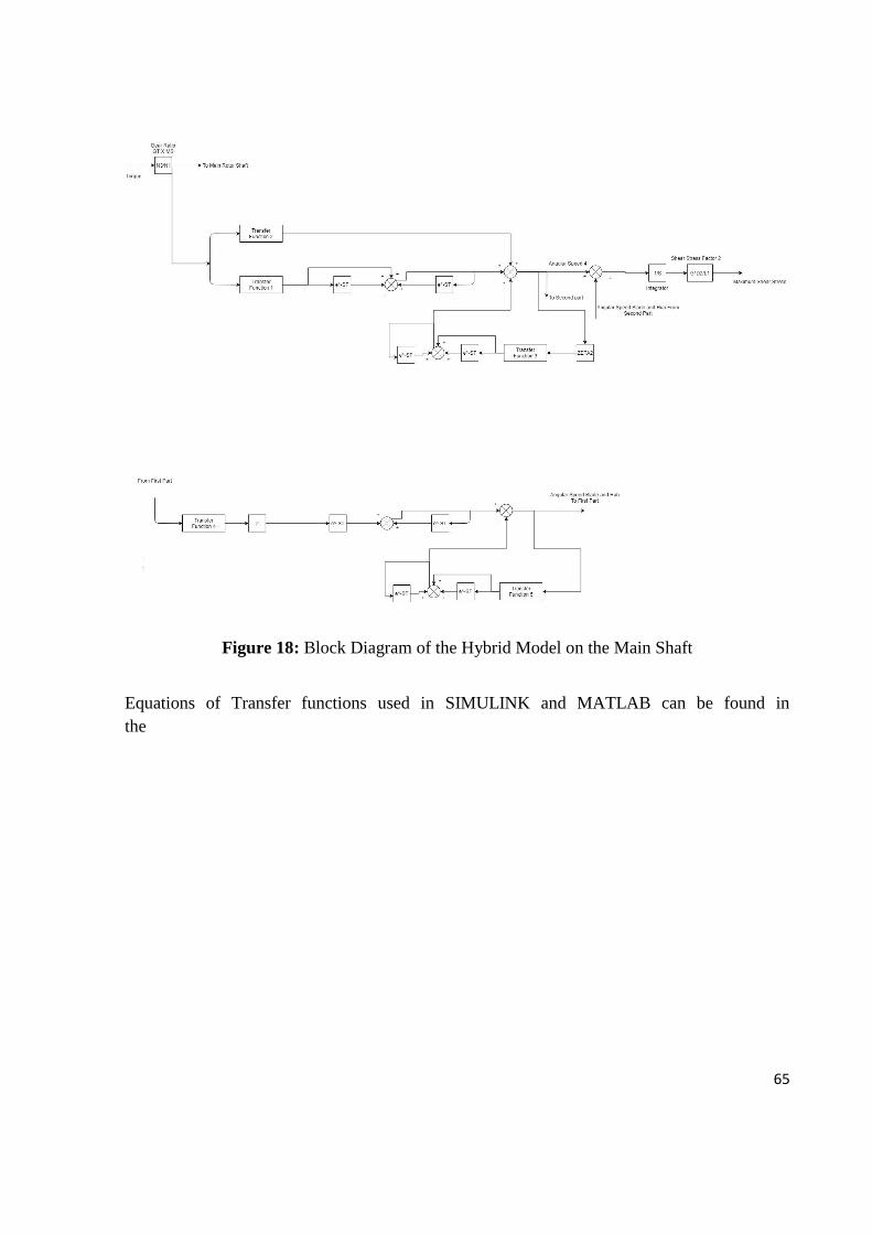
65

Figure 18: Block Diagram of the Hybrid Model on the Main Shaft


the

66

Appendix I.

3.5 Defining of Parameter Values & Equations for each Modeling Method

In this section, the results of the simulated responses including: the angular speeds,

the shear stress, the resonance speeds will be displayed. The behavior of the transfer

functions in terms of magnitude and decibels will also be shown (aka: the bode

plots). This section merely states the behavior, a thorough analysis and discussion is

shown in the Chapter 5.

But before any of the results, the design of each element for each type of model is

calculated:

The values for the design of gears, blades, hub, and shafts were taken from actual

values from different designs such as the R22 Robinson and CH53 Sikorsky;

depending on what was available. Values such as damping and density of the blade

alloy are estimated. This is because blade material for example is an alloy of

different metals depending on the manufacturer (trademark). However, this is not

meant to be a design and simulation of a specific helicopter model, but rather a

general simulation to the behavior of a helicopter transmission shafts.

3.5.1 Lumped Parameter Model Equations

Defining the density and depth of all gears:

𝐻 = 0.02 (3-232)

𝜌 = 7000 (3-133)

The density of the blades is estimated (Aluminum Alloy)

67

𝜌𝐵 = 3000 (3-234)

Main Rotor Shaft:

Shaft:

Inner and Outer Diameter:

𝐷1𝑀𝑆 = 𝑙0.0655 (3-5235)

𝐷2𝑀𝑆 = 0.07 (3-236)

The shaft is hollow in order to hold much more shear stress.

The Length:

𝐿1𝑀𝑆 = 3.96 (3-237)

The Polar Moment of Inertia (Mass):

𝐼1𝑀𝑆 = 𝜋 ∗ 𝜌 ∗ 𝐿1𝑀𝑆 ∗ (1

32) ∗ ((𝐷2𝑀𝑆

4 ) − (𝐷1𝑀𝑆4 ))

(3-238)

Gear 1:

Estimated Number of Teeth:

𝑁𝑇𝐷1 = 50 (3-239)


𝐷1𝐷1 = 0.08 (3-240)

𝐷2𝐷1 = 0.10 (3-241)


𝐼1 = 𝜋 ∗ 𝜌 ∗ 𝐻 ∗ (1

32) ∗ ((𝐷2𝐷1

4 ) − (𝐷1𝐷14 ))

(3-242)

Gear 2:


68

𝑁𝑇𝐷2 = 25 (3-243)


𝐷1𝐷2 = 0.08 (3-244)

𝐷2𝐷2 = 0.115 (3-245)


𝐼2 = 𝜋 ∗ 𝜌 ∗ 𝐻 ∗ (1

32) ∗ ((𝐷2𝐷2

4 ) − (𝐷1𝐷24 ))

(3-246)

Main Shaft:

Shaft:


𝐷1𝑀𝑅𝑆 = 0.042 (3-247)

𝐷2𝑀𝑅𝑆 = 0.05 (3-248)

The shaft is hollow in order to hold much more shear stress.

The Length:

𝐿1𝑀𝑅𝑆 = 1.34 (3-249)


𝐼1𝑀𝑅𝑆 = 𝜋 ∗ 𝜌 ∗ 𝐿1𝑀𝑅𝑆 ∗ (1

32) ∗ ((𝐷2𝑀𝑅𝑆

4 ) − (𝐷1𝑀𝑅𝑆4 ))

(3-250)

Gear 4:


𝑁𝑇𝐷4 = 60 (3-251)


𝐷1𝐷4 = 0.1 (3-252)

69

𝐷2𝐷4 = 0.11 (3-253)


𝐼4 = 𝜋 ∗ 𝜌 ∗ 𝐻 ∗ (1

32) ∗ ((𝐷2𝐷4

4 ) − (𝐷1𝐷44 ))

(3-254)

Blade and Hub 1:

Blade:

Estimated Number of Blades

𝑁𝐵1 = 5 (3-255)

Diameter of the blades (estimated to be very thin):

𝐷1𝐵1 = 0.02 (3-256)

The length of each blade:

𝐿𝐵1 = 4.03 (3-257)


𝐼𝐵1 = 𝑁𝐵1 ∗ 𝜋 ∗ 𝜌𝐵 ∗ 𝐿𝐵1 ∗ (1

32) ∗ (𝐷1𝐵1

4 ) (3-258)

Hub:

Hub Diameter:

𝐷𝐻1 = 0.1 (3-259)

Hub Depth:

𝐿𝐻1 = 0.35 (3-260)


𝐼𝐻1 = 𝜋 ∗ 𝜌𝐵 ∗ 𝐿𝐻1 ∗ (1

32) ∗ (𝐷𝐻1

4 ) (3-261)

Other Parameters of the Shafts

70

Main Rotor Shaft:

The Inertia:

𝐽1 = 𝐼1 (3-262)

𝐽2 = 𝐼2 (3-263)

𝐽1𝑀𝑆 = 𝐼1𝑀𝑆; (3-264)

The Damping:

𝐶1 = 2.5 (3-265)

𝐶2 = 20 (3-266)

The Modulus of Rigidity:

𝐺 = 80 ∗ 109 (3-267)

The Stiffness:

𝐾 =𝐺 ∗ 𝐽1𝑀𝑆

𝜌 ∗ (𝐿1𝑀𝑆2 )

; (3-268)

The Shear Stress Factor [Angle Difference is the signal]:

𝑆𝑆𝐹1 = 𝐺 ∗𝐷2𝑀𝑆

𝐿1𝑀𝑆;

(3-269)

Main Shaft:

The Inertia:

𝐽4 = 𝐼4 (3-270)

𝐽1𝐵1 = 𝐼𝐵1 (3-271)

𝐽𝐻1 = 𝐼𝐻1 (3-272)

𝐽1𝑀𝑅𝑆 = 𝐼1𝑀𝑅𝑆 (3-273)

𝐽𝐵1 = 𝐽1𝐵1 + 𝐽𝐻1 (3-274)

71

The Damping:

𝐶4 = 10 (3-275)

𝐶𝐵1 = 20 (3-276)

The Modulus of Rigidity:

𝐺 = 80 ∗ 109 (3-277)

The Stiffness:

𝐾𝑀𝑅𝑆 =𝐺 ∗ 𝐽1𝑀𝑅𝑆

𝜌 ∗ (𝐿1𝑀𝑅𝑆2 )

; (3-278)

The Shear Stress Factor:

𝑆𝑆𝐹2 = 𝐺 ∗𝐷2𝑀𝑅𝑆

𝐿1𝑀𝑅𝑆;

(3-279)

Gear Ratios:

Intermediate Shaft:

Gear 6:

Number of Teeth Estimated:

𝑁𝑇𝐷6 = 15 (3-280)

Gas Turbine Shaft:

Gear 3:


𝑁𝑇𝐷3 = 40 (3-281)

Tail Rotor Shaft:

Gear 5:


72

𝑁𝑇𝐷5 = 45 (3-282)

The Ratios:

Gas Turbine X Main Shaft:

𝐺𝑅𝐺𝑇𝑋𝑀𝑆 =𝑁𝑇𝐷3

𝑁𝑇𝐷1

(3-283)

Main Shaft x Tail Rotor Shaft:

𝐺𝑅𝑀𝑆𝑋𝑇𝑅𝑆 =𝑁𝑇𝐷2

𝑁𝑇𝐷5

(3-284)

Intermediate Shaft x Main Rotor Shaft:

𝐺𝑅𝐼𝑆𝑋𝑀𝑅𝑆 =𝑁𝑇𝐷6

𝑁𝑇𝐷4

(3-285)

Torque:

The Torque of the gas turbine is modeled as a 6000rpm turbo shaft:

Conversion to Hz, the Angular speed is:

𝑊𝑇 = 6000 ∗ 2 ∗𝜋

60 (3-286)

The Turbo shaft engine is modeled to have 350 Horse Power:

Conversion to kW, the Power is:

𝑃𝑇 = 350 ∗ 745.7 (3-287)

The Torque Equation is:

𝑇𝑇 =𝑃𝑇

𝑊𝑇

(3-288)

Resonance:

Resonance of the shaft is given by the derived equations:

At End 1:

73

𝑤 = √𝐾 ∗ (𝐶1 + 𝐶2)

(𝐽1 ∗ 𝐶2) + (𝐽2 ∗ 𝐶1)

(3-289)

At End 2:

𝑤2 = √𝐾𝑀𝑅𝑆 ∗ (𝐶4 + 𝐶𝐵1)

(𝐽4 ∗ 𝐶𝐵1) + (𝐽𝐵1 ∗ 𝐶4);

(3-290)

Calculated Values:

𝐽1 = 8.1147𝑒 − 04 (3-291)

𝐽2 = 0.0018 (3-292)

𝐾 = 1.1114𝑒 + 04 (3-293)

𝐽4 = 6.3788𝑒 − 04 (3-294)

𝐽𝐵1 = 0.0113 (3-295)

𝐾𝑀𝑅𝑆 = 1.8394𝑒 + 04 (3-296)

𝐽1𝑀𝑆 = 0.0153 (3-297)

𝐽1𝑀𝑅𝑆 = 0.0029 (3-298)

𝐺𝑅𝐺𝑇𝑋𝑀𝑆 = 0.8000 (3-299)

𝐺𝑅𝑀𝑆𝑋𝑇𝑅𝑆 = 0.5556 (3-300)

𝐺𝑅𝐼𝑆𝑋𝑀𝑅𝑆 = 0.2500 (3-301)

𝑇𝑇 = 415.3864 (3-302)

𝑆𝑆𝐹1 = 1.4141𝑒 + 09 (3-303)

𝑆𝑆𝐹2 = 2.9851𝑒 + 09 (3-304)

𝑊 = 828.8999 (3-305)

𝑊2 = 1.6132𝑒 + 03 (3-306)

74

3.5.2 Finite Element Model Equations

Main Rotor Shaft:

Setting the variables of the system:

𝑠𝑦𝑚𝑠 𝑆 𝑇1 𝑇2 𝐶1 𝐶2 𝐽1 𝐽2 𝐽 𝐾 (3-307)

Properties of finite elements:

𝐾 = 5 ∗ 𝐾 (3-308)

𝐽 =𝐽1𝑀𝑆

5

(3-309)

The A Matrix is composed of:

𝐾𝐹 = [𝐾 − 𝐾 0 0 0 0; −𝐾 𝐾 + 𝐾 − 𝐾 0 0 0; 0 − 𝐾 𝐾 + 𝐾 − 𝐾 0 0; 0 0

− 𝐾 𝐾 + 𝐾 − 𝐾 0; 0 0 0 − 𝐾 𝐾 + 𝐾 − 𝐾; 0 0 0 0 − 𝐾 𝐾]

(3-310)

𝐶

= [𝐶1 0 0 0 0 0; 0 0 0 0 0 0; 0 0 0 0 0 0; 0 0 0 0 0 0; 0 0 0 0 0 0; 0 0 0 0 0 𝐶2]

(3-311)

𝐽𝐹

= [𝐽1 0 0 0 0 0; 0 𝐽 0 0 0 0; 0 0 𝐽 0 0 0; 0 0 0 𝐽 0 0; 0 0 0 0 𝐽 0; 0 0 0 0 0 𝐽2];

(3-312)

𝐴1 = 𝐽𝐹 ∗ 𝑆2 (3-313)

𝐴2 = 𝐶 ∗ 𝑆 (3-314)

𝐴3 = 𝐾𝐹 (3-315)

𝐴 = 𝐴1 + 𝐴2 + 𝐴3 (3-316)

The Inverse of A Matrix:

𝑌 = 𝑖𝑛𝑣 (𝐴) (3-317)

The Torque Vector:

75

𝑇 = [𝑇1; 0; 0; 0; 0; 0]; (3-318)

The Angular Speed Vector:

𝑊𝐹 = 𝑌 ∗ 𝑇 (3-319)

After obtaining the equations in variable form, the variables are re arranged in terms

of S, in a matrix form:

Matrix X:

𝑋1 = ((𝐾5) ∗ 𝐽2) + (4 ∗ (𝐾5) ∗ 𝐽) + ((𝐾5) ∗ 𝐽1) + (5 ∗ (𝐾4) ∗ 𝐶1 ∗ 𝐶2) (3-320)

𝑋2 = (5 ∗ (𝐾4) ∗ 𝐶1 ∗ 𝐽2) + (10 ∗ (𝐾4) ∗ 𝐽 ∗ 𝐶2) + (5 ∗ (𝐾4) ∗ 𝐽1 ∗ 𝐶2)

+ (10 ∗ (𝐾4) ∗ 𝐶1 ∗ 𝐽)

(3-321)

𝑋3 = (5 ∗ (𝐾4) ∗ 𝐽1 ∗ 𝐽2) + (20 ∗ (𝐾3) ∗ 𝐶1 ∗ 𝐽 ∗ 𝐶2) + (10 ∗ (𝐾4) ∗ 𝐽1

∗ 𝐽) + (10 ∗ (𝐽2) ∗ (𝐾4)) + (10 ∗ (𝐾4) ∗ 𝐽 ∗ 𝐽2)

(3-322)

𝑋4 = (15 ∗ (𝐾3) ∗ 𝐶1 ∗ (𝐽2)) + (15 ∗ (𝐾3) ∗ (𝐽2) ∗ 𝐶2) + (20 ∗ (𝐾3)

∗ 𝐶1 ∗ 𝐽 ∗ 𝐽2) + (20 ∗ (𝐾3) ∗ 𝐽1 ∗ 𝐽 ∗ 𝐶2)

(3-323)

𝑋5 = (15 ∗ (𝐾3) ∗ (𝐽2) ∗ 𝐽2) + (20 ∗ (𝐾3) ∗ 𝐽1 ∗ 𝐽 ∗ 𝐽2) + (6 ∗ (𝐽3)

∗ (𝐾3)) + (15 ∗ (𝐾3) ∗ 𝐽1 ∗ (𝐽2)) + (21 ∗ (𝐾2) ∗ 𝐶1

∗ (𝐽2) ∗ 𝐶2)

(3-324)

𝑋6 = (21 ∗ (𝐾2) ∗ 𝐽1 ∗ (𝐽2) ∗ 𝐶2) + (7 ∗ 𝐶1 ∗ (𝐽3) ∗ (𝐾2)) + (21 ∗ (𝐾2)

∗ 𝐶1 ∗ (𝐽2) ∗ 𝐽2) + (7 ∗ (𝐾2) ∗ (𝐽3) ∗ 𝐶2);

(3-325)

𝑋7 = (7 ∗ 𝐽1 ∗ (𝐽3) ∗ (𝐾2)) + (21 ∗ (𝐾2) ∗ 𝐽1 ∗ (𝐽2) ∗ 𝐽2) + ((𝐾2)

∗ (𝐽4)) + (8 ∗ 𝐾 ∗ 𝐶1 ∗ (𝐽3) ∗ 𝐶2) + (7 ∗ (𝐾2) ∗ (𝐽3) ∗ 𝐽2)

(3-326)

𝑋8 = (𝐾 ∗ 𝐶1 ∗ (𝐽4)) + (8 ∗ 𝐾 ∗ 𝐶1 ∗ (𝐽3) ∗ 𝐽2) + (8 ∗ 𝐾 ∗ 𝐽1 ∗ (𝐽3)

∗ 𝐶2) + (𝐾 ∗ (𝐽4) ∗ 𝐶2)

(3-327)

76

𝑋9 = (𝐾 ∗ (𝐽4) ∗ 𝐽2) + (8 ∗ 𝐾 ∗ 𝐽1 ∗ (𝐽3) ∗ 𝐽2) + (𝐾 ∗ 𝐽1 ∗ (𝐽4)) + (𝐶1

∗ (𝐽4) ∗ 𝐶2)

(3-328)

𝑋10 = (𝐶1 ∗ (𝐽4) ∗ 𝐽2) + (𝐽1 ∗ (𝐽4) ∗ 𝐶2) (3-329)

𝑋11 = (𝐽1 ∗ (𝐽4) ∗ 𝐽2) (3-330)

Matrix Y:

𝑌0 = (𝐾5) (3-331)

𝑌1 = (5 ∗ (𝐾4) ∗ 𝐶2) (3-332)

𝑌2 = (5 ∗ (𝐾4) ∗ 𝐽2) + (10 ∗ (𝐾4) ∗ 𝐽) (3-333)

𝑌3 = (20 ∗ (𝐾3) ∗ 𝐽 ∗ 𝐶2) (3-334)

𝑌4 = (15 ∗ (𝐾3) ∗ (𝐽2)) + (20 ∗ (𝐾3) ∗ 𝐽 ∗ 𝐽2) (3-335)

𝑌5 = (21 ∗ (𝐾2) ∗ (𝐽2) ∗ 𝐶2) (3-336)

𝑌6 = (7 ∗ (𝐽3) ∗ (𝐾2)) + (21 ∗ (𝐾2) ∗ (𝐽2) ∗ 𝐽2) (3-337)

𝑌7 = (8 ∗ 𝐾 ∗ (𝐽3) ∗ 𝐶2) (3-338)

𝑌8 = (8 ∗ 𝐾 ∗ (𝐽3) ∗ 𝐽2) + (𝐾 ∗ (𝐽4)) (3-339)

𝑌9 = ((𝐽4) ∗ 𝐶2) (3-10)

𝑌10 = ((𝐽4) ∗ 𝐽2) (3-341)

Main Shaft:

Setting the variables of the system:

𝑠𝑦𝑚𝑠 𝑆 𝑇22 𝑇2 𝐶4 𝐶𝐵1 𝐽4 𝐽𝐵1 𝐽22 𝐾𝑀𝑅𝑆 (3-342)

Properties of finite elements:

𝐾𝑀𝑅𝑆 = 5 ∗ 𝐾𝑀𝑅𝑆 (3-342)

77

𝐽22 =𝐽1𝑀𝑅𝑆

5

(3-343)

The A Matrix is composed of:

𝐾𝐹2 = [𝐾𝑀𝑅𝑆 − 𝐾𝑀𝑅𝑆 0 0 0 0; −𝐾𝑀𝑅𝑆 𝐾𝑀𝑅𝑆 + 𝐾𝑀𝑅𝑆 − 𝐾𝑀𝑅𝑆 0 0 0; 0

− 𝐾𝑀𝑅𝑆 𝐾𝑀𝑅𝑆 + 𝐾𝑀𝑅𝑆 − 𝐾𝑀𝑅𝑆 0 0; 0 0 − 𝐾𝑀𝑅𝑆 𝐾𝑀𝑅𝑆

+ 𝐾𝑀𝑅𝑆 − 𝐾𝑀𝑅𝑆 0; 0 0 0 − 𝐾𝑀𝑅𝑆 𝐾𝑀𝑅𝑆 + 𝐾𝑀𝑅𝑆

− 𝐾𝑀𝑅𝑆; 0 0 0 0 − 𝐾𝑀𝑅𝑆 𝐾𝑀𝑅𝑆];

(3-344)

𝐶22 = [𝐶4 0 0 0 0 0; 0 0 0 0 0 0; 0 0 0 0 0 0; 0 0 0 0 0 0; 0 0 0 0 0 𝐶𝐵1]; (3-345)

𝐽𝐹2 = [𝐽4 0 0 0 0 0; 0 𝐽22 0 0 0 0; 0 0 𝐽22 0 0 0; 0 0 0 𝐽22 0 0;

0 0 0 0 𝐽22 0; 0 0 0 0 0 𝐽𝐵1];

(3-346)

𝐴4 = 𝐽𝐹2 ∗ 𝑆2 (3-347)

𝐴5 = 𝐶22 ∗ 𝑆

𝐴6 = 𝐾𝐹2 (1)

𝐴22 = 𝐴4 + 𝐴5 + 𝐴6 (2)

(3-348)

The Inverse of A Matrix:

𝑌22 = 𝑖𝑛𝑣 (𝐴22) (3-349)

The Torque Vector:

𝑇22 = [𝑇2; 0; 0; 0; 0; 0]; (3-350)

The Angular Speed Vector:

𝑊𝐹2 = 𝑌22 ∗ 𝑇22 (3-351)

After obtaining the equations in variable form, the variables are re arranged in terms

of S, in a matrix form:

Matrix V:

78

𝑉0 = ((𝐾5) ∗ 𝐶4) + ((𝐾5) ∗ 𝐶𝐵1) (3-352)

𝑉1 = ((𝐾5) ∗ 𝐽𝐵1) + (4 ∗ (𝐾5) ∗ 𝐽) + ((𝐾5) ∗ 𝐽4) + (5 ∗ (𝐾4) ∗ 𝐶4

∗ 𝐶𝐵1)

(3-353)

𝑉2 = (5 ∗ (𝐾4) ∗ 𝐶4 ∗ 𝐽𝐵1) + (10 ∗ (𝐾4) ∗ 𝐽 ∗ 𝐶𝐵1) + (5 ∗ (𝐾4) ∗ 𝐽4

∗ 𝐶𝐵1) + (10 ∗ (𝐾4) ∗ 𝐶4 ∗ 𝐽)

(3-354)

𝑉3 = (5 ∗ (𝐾4) ∗ 𝐽4 ∗ 𝐽𝐵1) + (20 ∗ (𝐾3) ∗ 𝐶4 ∗ 𝐽 ∗ 𝐶𝐵1) + (10 ∗ (𝐾4)

∗ 𝐽4 ∗ 𝐽) + (10 ∗ (𝐽2) ∗ (𝐾4)) + (10 ∗ (𝐾4) ∗ 𝐽 ∗ 𝐽𝐵1)

(3-355)

𝑉4 = (15 ∗ (𝐾3) ∗ 𝐶4 ∗ (𝐽2)) + (15 ∗ (𝐾3) ∗ (𝐽2) ∗ 𝐶𝐵1) + (20 ∗ (𝐾3)

∗ 𝐶4 ∗ 𝐽 ∗ 𝐽𝐵1) + (20 ∗ (𝐾3) ∗ 𝐽4 ∗ 𝐽 ∗ 𝐶𝐵1)

(3-356)

𝑉5 = (15 ∗ (𝐾3) ∗ (𝐽2) ∗ 𝐽𝐵1) + (20 ∗ (𝐾3) ∗ 𝐽4 ∗ 𝐽 ∗ 𝐽𝐵1) + (6 ∗ (𝐽3)

∗ (𝐾3)) + (15 ∗ (𝐾3) ∗ 𝐽4 ∗ (𝐽2)) + (21 ∗ (𝐾2) ∗ 𝐶4 ∗ (𝐽2)

∗ 𝐶𝐵1)

(3-357)

𝑉6 = (21 ∗ (𝐾2) ∗ 𝐽4 ∗ (𝐽2) ∗ 𝐶𝐵1) + (7 ∗ 𝐶4 ∗ (𝐽3) ∗ (𝐾2)) + (21

∗ (𝐾2) ∗ 𝐶4 ∗ (𝐽2) ∗ 𝐽𝐵1) + (7 ∗ (𝐾2) ∗ (𝐽3) ∗ 𝐶𝐵1)

(3-358)

𝑉7 = (7 ∗ 𝐽4 ∗ (𝐽3) ∗ (𝐾2)) + (21 ∗ (𝐾2) ∗ 𝐽4 ∗ (𝐽2) ∗ 𝐽𝐵1) + ((𝐾2)

∗ (𝐽4)) + (8 ∗ 𝐾 ∗ 𝐶4 ∗ (𝐽3) ∗ 𝐶𝐵1) + (7 ∗ (𝐾2) ∗ (𝐽3)

∗ 𝐽𝐵1)

(3-359)

𝑉8 = (𝐾 ∗ 𝐶4 ∗ (𝐽4)) + (8 ∗ 𝐾 ∗ 𝐶4 ∗ (𝐽3) ∗ 𝐽𝐵1) + (8 ∗ 𝐾 ∗ 𝐽4 ∗ (𝐽3)

∗ 𝐶𝐵1) + (𝐾 ∗ (𝐽4) ∗ 𝐶𝐵1)

(3-5360)

𝑉9 = (𝐾 ∗ (𝐽4) ∗ 𝐽𝐵1) + (8 ∗ 𝐾 ∗ 𝐽4 ∗ (𝐽3) ∗ 𝐽𝐵1) + (𝐾 ∗ 𝐽4 ∗ (𝐽4))

+ (𝐶4 ∗ (𝐽4) ∗ 𝐶𝐵1)

(3-361)

𝑉10 = (𝐶4 ∗ (𝐽4) ∗ 𝐽𝐵1) + (𝐽4 ∗ (𝐽4) ∗ 𝐶𝐵1) (3-362)

79

𝑉11 = (𝐽4 ∗ (𝐽4) ∗ 𝐽𝐵1) (3-363)

Matrix W:

𝑊0 = (𝐾5) (3-364)

𝑊1 = (5 ∗ (𝐾4) ∗ 𝐶𝐵1) (3-365)

𝑊2 = (5 ∗ (𝐾4) ∗ 𝐽𝐵1) + (10 ∗ (𝐾4) ∗ 𝐽) (3-366)

𝑊3 = (20 ∗ (𝐾3) ∗ 𝐽 ∗ 𝐶𝐵1) (3-367)

𝑊4 = (15 ∗ (𝐾3) ∗ (𝐽2)) + (20 ∗ (𝐾3) ∗ 𝐽 ∗ 𝐽𝐵1) (3-368)

𝑊5 = (21 ∗ (𝐾2) ∗ (𝐽2) ∗ 𝐶𝐵1) (3-369)

𝑊6 = (7 ∗ (𝐽3) ∗ (𝐾2)) + (21 ∗ (𝐾2) ∗ (𝐽2) ∗ 𝐽𝐵1) (3-370)

𝑊7 = (8 ∗ 𝐾 ∗ (𝐽3) ∗ 𝐶𝐵1) (3-371)

𝑊8 = (8 ∗ 𝐾 ∗ (𝐽3) ∗ 𝐽𝐵1) + (𝐾 ∗ (𝐽4)) (3-372)

𝑊9 = ((𝐽4) ∗ 𝐶𝐵1) (3-373)

𝑊10 = ((𝐽4) ∗ 𝐽𝐵1) (3-374)

Resonance Equations:

𝑤3 = [−𝑋10 0 𝑋8 0 − 𝑋6 0 𝑋4 0 − 𝑋2 0 𝑋0] (3-375)

𝑤4 = [−𝑉10 0 𝑉8 0 − 𝑉6 0 𝑉4 0 − 𝑉2 0 𝑉0] (3-376)

𝑟𝑜𝑜𝑡𝑠(𝑤3);

𝑟𝑜𝑜𝑡𝑠(𝑤4);

Only real positive values are taken into consideration.

3.5.3 Hybrid (Distributed-Lumped) Model Equations

Main Rotor Shaft:

System Characteristics:

80

Compliance/Inverse of Stiffness (Equivalent to Capacitance):

𝐶𝑂𝑀1 =𝜌 ∗ 𝐿1𝑀𝑆

𝐺 ∗ 𝐽1𝑀𝑆

(3-377)

Inductance (Equivalent to Polar moment of inertia, mass):

𝐿𝐼𝑁1 =𝐽1𝑀𝑆

𝐿1𝑀𝑆

(3-378)

The Impedance:

𝜁1 = √(𝐿𝐼𝑁1

𝐶𝑂𝑀1)

(3-379)

Time Constants and Delays:

𝜏𝑠1 = √𝐿𝐼𝑁1 ∗ 𝐶𝑂𝑀1 (3-380)

𝜏1 = 2 ∗ 𝐿1𝑀𝑆 ∗ 𝑇𝐴𝑊𝑆1 (3-381)

Transfer Function Equivalence Equations (For Convenience):

𝛾11 = [𝐽1 𝐶1] (3-382)

𝛾12 = [𝐽2 𝐶2] (3-383)

𝐷𝑆11 = 𝐽1 ∗ 𝐽2 (3-384)

𝐷𝑆12 = (𝐽1 ∗ 𝐶2) + (𝐽2 ∗ 𝐶1) (3-385)

𝐷𝑆13 = (𝐶1 ∗ 𝐶2) + (𝜁12) (3-386)

Main Shaft:

System Characteristics:

Compliance/Inverse of Stiffness (Equivalent to Capacitance):

𝐶𝑂𝑀2 =𝜌 ∗ 𝐿1𝑀𝑅𝑆

𝐺 ∗ 𝐽1𝑀𝑅𝑆

(3-387)

Inductance (Equivalent to Polar moment of inertia, mass):

81

𝐿𝐼𝑁2 =𝐽1𝑀𝑅𝑆

𝐿1𝑀𝑅𝑆

(3-388)

The Impedance:

𝜁2 = √(𝐿𝐼𝑁2

𝐶𝑂𝑀2)

(3-389)

Time Constants and Delays:

𝜏𝑠2 = √𝐿𝐼𝑁2 ∗ 𝐶𝑂𝑀2 (3-390)

𝜏2 = 2 ∗ 𝐿1𝑀𝑅𝑆 ∗ 𝑇𝐴𝑊𝑆2 (3-391)

Transfer Function Equivalence Equations (For Convenience):

𝛾21 = [𝐽4 𝐶4] (3-392)

𝛾22 = [𝐽𝐵1 𝐶𝐵1] (3-393)

𝐷𝑆21 = 𝐽4 ∗ 𝐽𝐵1 (3-394)

𝐷𝑆22 = (𝐽4 ∗ 𝐶𝐵1) + (𝐽𝐵1 ∗ 𝐶4) (3-395)

𝐷𝑆23 = (𝐶4 ∗ 𝐶𝐵1) + (𝜁22)

(3-396)

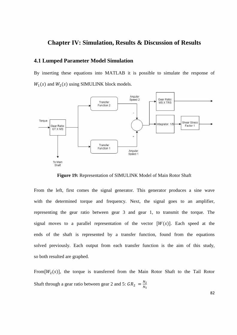
82

Chapter IV: Simulation, Results & Discussion of Results

4.1 Lumped Parameter Model Simulation

By inserting these equations into MATLAB it is possible to simulate the response of

𝑊1(𝑠) and 𝑊2(𝑠) using SIMULINK block models.

Figure 19: Representation of SIMULINK Model of Main Rotor Shaft

From the left, first comes the signal generator. This generator produces a sine wave

with the determined torque and frequency. Next, the signal goes to an amplifier,

representing the gear ratio between gear 3 and gear 1, to transmit the torque. The

signal moves to a parallel representation of the vector [𝑊(𝑠)]. Each speed at the

ends of the shaft is represented by a transfer function, found from the equations

solved previously. Each output from each transfer function is the aim of this study,

so both resulted are graphed.

From[𝑊2(𝑠)], the torque is transferred from the Main Rotor Shaft to the Tail Rotor

Shaft through a gear ratio between gear 2 and 5: 𝐺𝑅2 =𝑁2

𝑁5

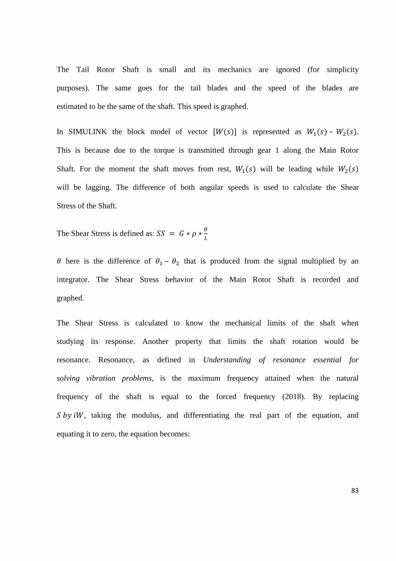
83

The Tail Rotor Shaft is small and its mechanics are ignored (for simplicity

purposes). The same goes for the tail blades and the speed of the blades are

estimated to be the same of the shaft. This speed is graphed.

In SIMULINK the block model of vector [𝑊(𝑠)] is represented as 𝑊1(𝑠) – 𝑊2(𝑠).

This is because due to the torque is transmitted through gear 1 along the Main Rotor

Shaft. For the moment the shaft moves from rest, 𝑊1(𝑠) will be leading while 𝑊2(𝑠)

will be lagging. The difference of both angular speeds is used to calculate the Shear

Stress of the Shaft.

The Shear Stress is defined as: 𝑆𝑆 = 𝐺 ∗ 𝜌 ∗𝜃

𝐿

𝜃 here is the difference of 𝜃1 – 𝜃2 that is produced from the signal multiplied by an

integrator. The Shear Stress behavior of the Main Rotor Shaft is recorded and

graphed.

The Shear Stress is calculated to know the mechanical limits of the shaft when

studying its response. Another property that limits the shaft rotation would be

resonance. Resonance, as defined in Understanding of resonance essential for

solving vibration problems, is the maximum frequency attained when the natural

frequency of the shaft is equal to the forced frequency (2018). By replacing

𝑆 𝑏𝑦 𝑖𝑊, taking the modulus, and differentiating the real part of the equation, and

equating it to zero, the equation becomes:

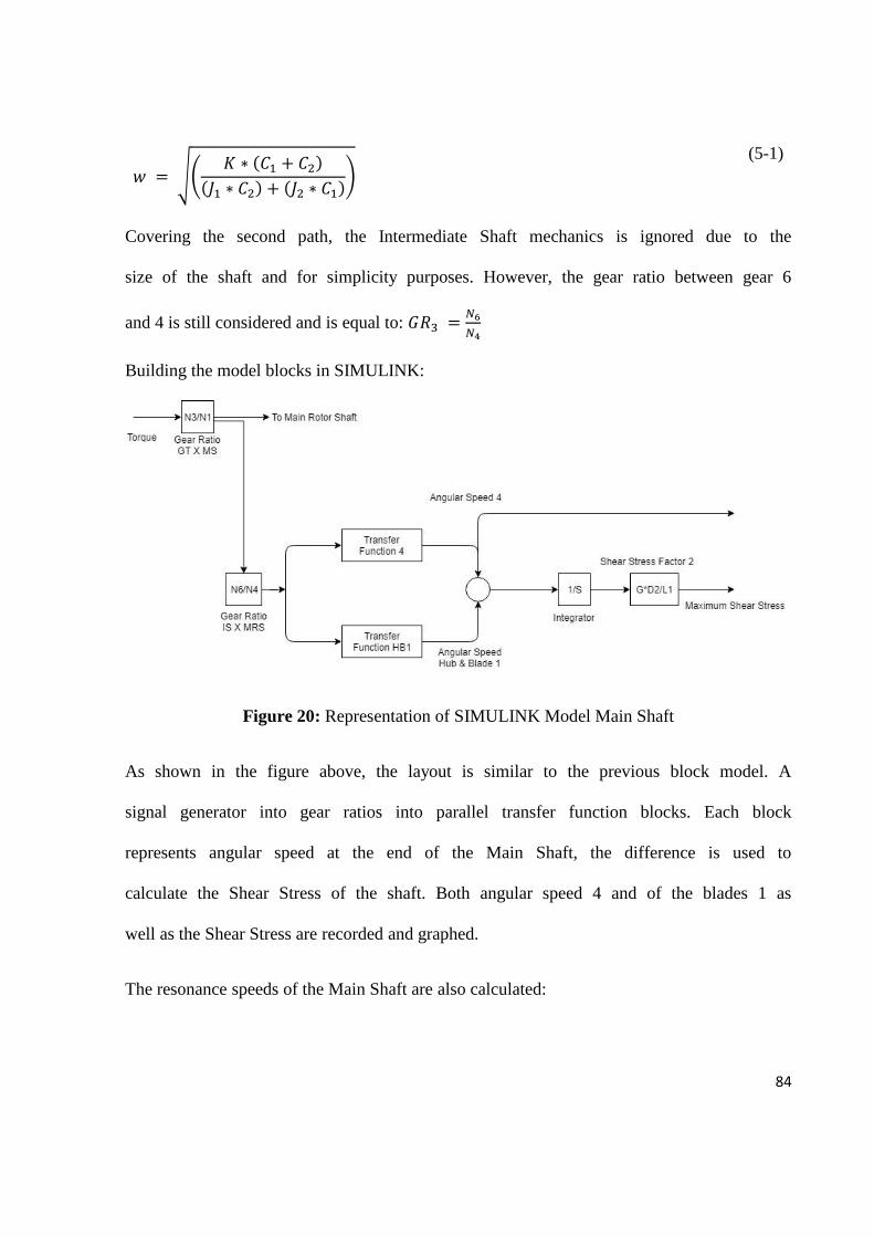
84

𝑤 = √(𝐾 ∗ (𝐶1 + 𝐶2)

(𝐽1 ∗ 𝐶2) + (𝐽2 ∗ 𝐶1))

(5-1)

Covering the second path, the Intermediate Shaft mechanics is ignored due to the

size of the shaft and for simplicity purposes. However, the gear ratio between gear 6

and 4 is still considered and is equal to: 𝐺𝑅3 =𝑁6

𝑁4

Building the model blocks in SIMULINK:

Figure 20: Representation of SIMULINK Model Main Shaft

As shown in the figure above, the layout is similar to the previous block model. A

signal generator into gear ratios into parallel transfer function blocks. Each block

represents angular speed at the end of the Main Shaft, the difference is used to

calculate the Shear Stress of the shaft. Both angular speed 4 and of the blades 1 as

well as the Shear Stress are recorded and graphed.

The resonance speeds of the Main Shaft are also calculated:

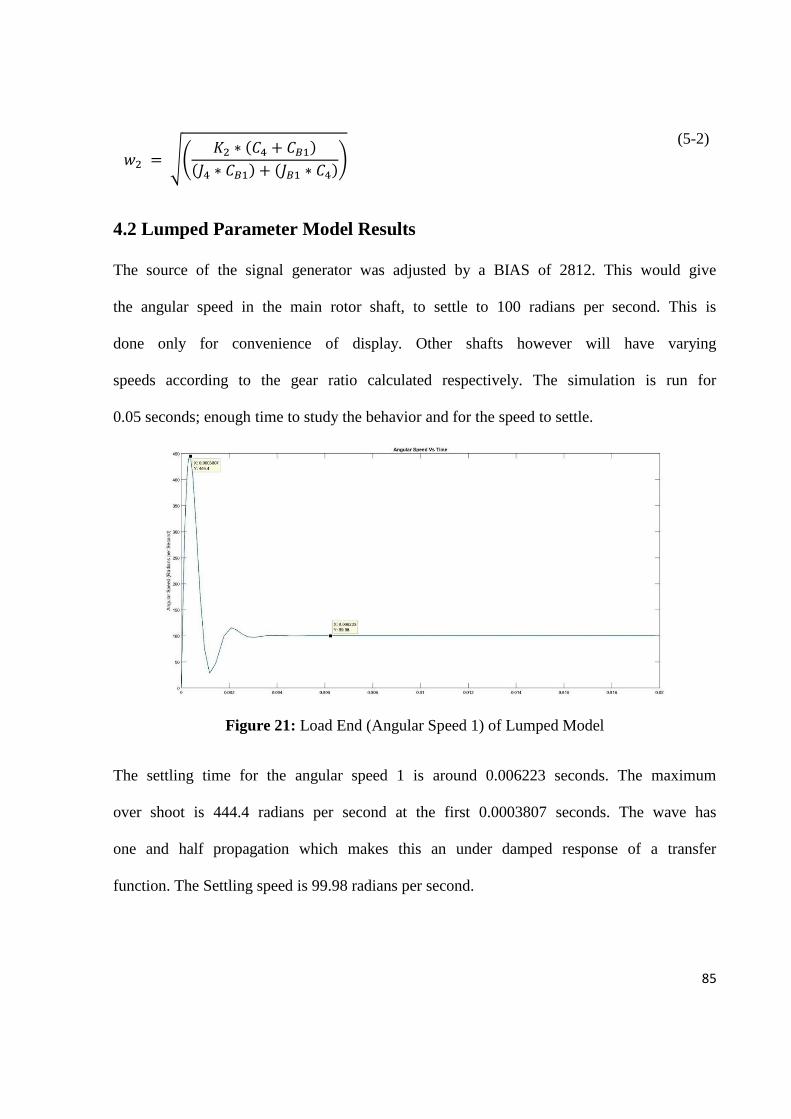
85

𝑤2 = √(𝐾2 ∗ (𝐶4 + 𝐶𝐵1)

(𝐽4 ∗ 𝐶𝐵1) + (𝐽𝐵1 ∗ 𝐶4))

(5-2)

4.2 Lumped Parameter Model Results

The source of the signal generator was adjusted by a BIAS of 2812. This would give

the angular speed in the main rotor shaft, to settle to 100 radians per second. This is

done only for convenience of display. Other shafts however will have varying

speeds according to the gear ratio calculated respectively. The simulation is run for

0.05 seconds; enough time to study the behavior and for the speed to settle.

Figure 21: Load End (Angular Speed 1) of Lumped Model

The settling time for the angular speed 1 is around 0.006223 seconds. The maximum

over shoot is 444.4 radians per second at the first 0.0003807 seconds. The wave has

one and half propagation which makes this an under damped response of a transfer

function. The Settling speed is 99.98 radians per second.

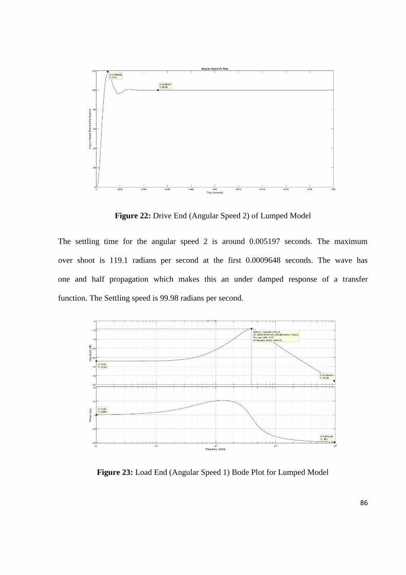
86

Figure 22: Drive End (Angular Speed 2) of Lumped Model





Figure 23: Load End (Angular Speed 1) Bode Plot for Lumped Model

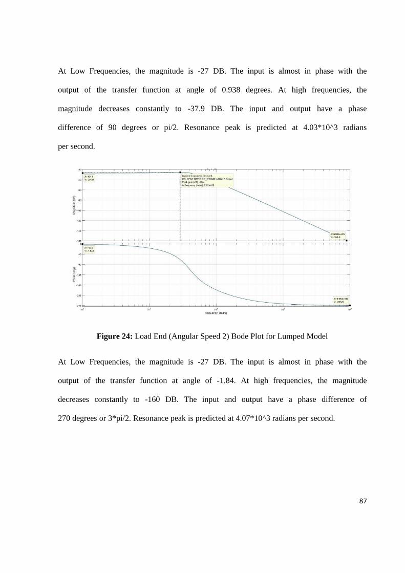
87

At Low Frequencies, the magnitude is -27 DB. The input is almost in phase with the

output of the transfer function at angle of 0.938 degrees. At high frequencies, the

magnitude decreases constantly to -37.9 DB. The input and output have a phase

difference of 90 degrees or pi/2. Resonance peak is predicted at 4.03*10^3 radians

per second.

Figure 24: Load End (Angular Speed 2) Bode Plot for Lumped Model

At Low Frequencies, the magnitude is -27 DB. The input is almost in phase with the

output of the transfer function at angle of -1.84. At high frequencies, the magnitude

decreases constantly to -160 DB. The input and output have a phase difference of

270 degrees or 3*pi/2. Resonance peak is predicted at 4.07*10^3 radians per second.

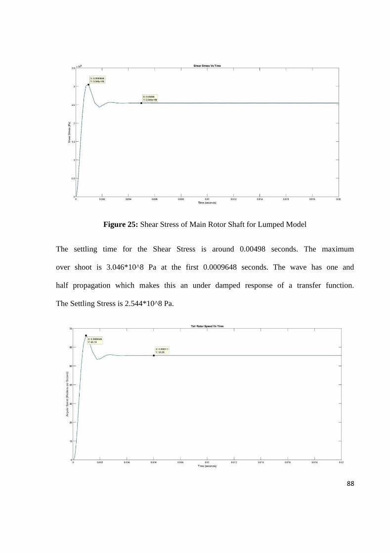
88

Figure 25: Shear Stress of Main Rotor Shaft for Lumped Model

The settling time for the Shear Stress is around 0.00498 seconds. The maximum

over shoot is 3.046*10^8 Pa at the first 0.0009648 seconds. The wave has one and

half propagation which makes this an under damped response of a transfer function.

The Settling Stress is 2.544*10^8 Pa.

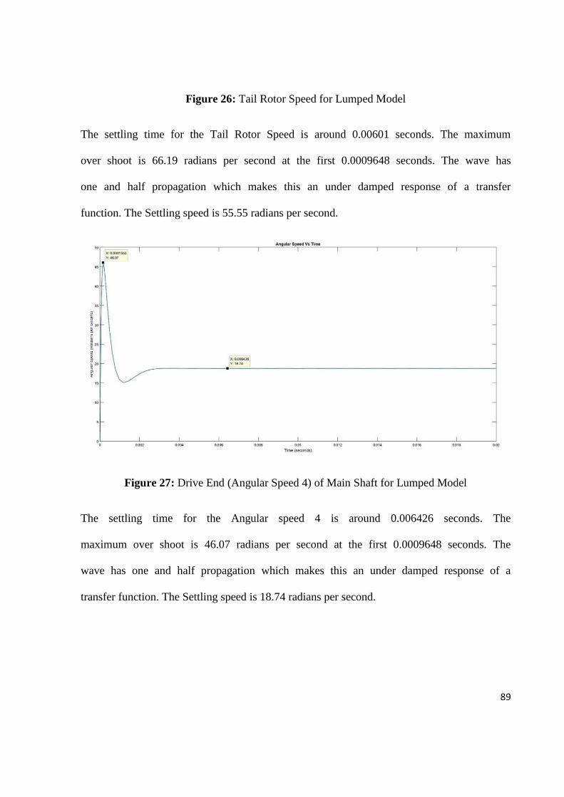
89

Figure 26: Tail Rotor Speed for Lumped Model

The settling time for the Tail Rotor Speed is around 0.00601 seconds. The maximum




Figure 27: Drive End (Angular Speed 4) of Main Shaft for Lumped Model

The settling time for the Angular speed 4 is around 0.006426 seconds. The

maximum over shoot is 46.07 radians per second at the first 0.0009648 seconds. The

wave has one and half propagation which makes this an under damped response of a

transfer function. The Settling speed is 18.74 radians per second.

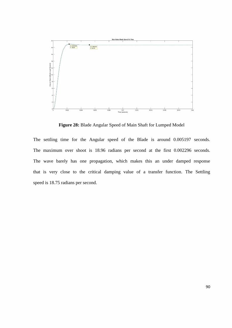
90

Figure 28: Blade Angular Speed of Main Shaft for Lumped Model

The settling time for the Angular speed of the Blade is around 0.005197 seconds.

The maximum over shoot is 18.96 radians per second at the first 0.002296 seconds.

The wave barely has one propagation, which makes this an under damped response

that is very close to the critical damping value of a transfer function. The Settling

speed is 18.75 radians per second.

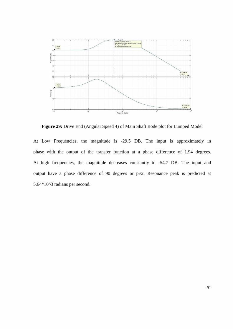
91

Figure 29: Drive End (Angular Speed 4) of Main Shaft Bode plot for Lumped Model

At Low Frequencies, the magnitude is -29.5 DB. The input is approximately in

phase with the output of the transfer function at a phase difference of 1.94 degrees.

At high frequencies, the magnitude decreases constantly to -54.7 DB. The input and

output have a phase difference of 90 degrees or pi/2. Resonance peak is predicted at

5.64*10^3 radians per second.

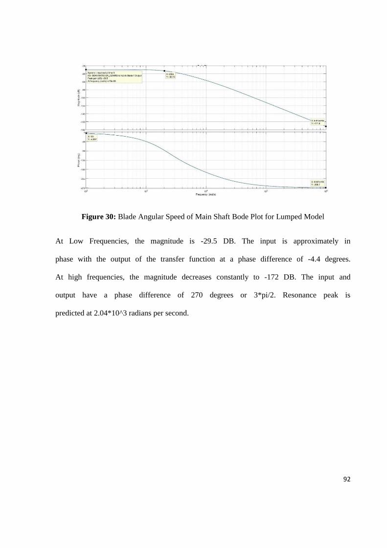
92

Figure 30: Blade Angular Speed of Main Shaft Bode Plot for Lumped Model


phase with the output of the transfer function at a phase difference of -4.4 degrees.

At high frequencies, the magnitude decreases constantly to -172 DB. The input and

output have a phase difference of 270 degrees or 3*pi/2. Resonance peak is

predicted at 2.04*10^3 radians per second.

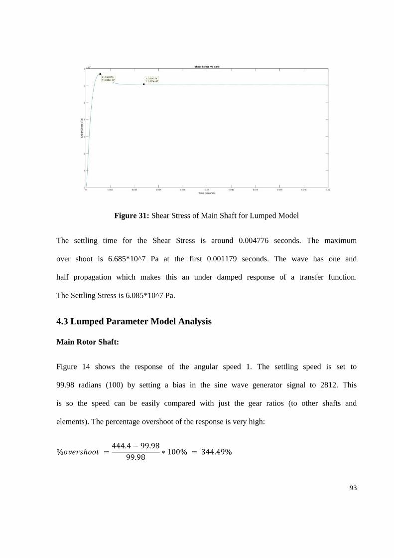
93

Figure 31: Shear Stress of Main Shaft for Lumped Model


over shoot is 6.685*10^7 Pa at the first 0.001179 seconds. The wave has one and

half propagation which makes this an under damped response of a transfer function.

The Settling Stress is 6.085*10^7 Pa.

4.3 Lumped Parameter Model Analysis

Main Rotor Shaft:

Figure 14 shows the response of the angular speed 1. The settling speed is set to

99.98 radians (100) by setting a bias in the sine wave generator signal to 2812. This

is so the speed can be easily compared with just the gear ratios (to other shafts and

elements). The percentage overshoot of the response is very high:

%𝑜𝑣𝑒𝑟𝑠ℎ𝑜𝑜𝑡 =444.4 − 99.98

99.98∗ 100% = 344.49%

94

This corresponding to R.Whalley’s and M.Ibrahimi’s work where they reach an over

shoot of 80% (April, 2005). Both results being outliers to a typical stable system

where the % overshoot would be a lot lower. The discrepancy between the results is

a matter of shaft and gear design as well the system application. A high % overshoot

is usually followed by tendency to either instability of the system, or a very high

maximum shear stress where the shaft breaks due to forces of rotation. Neither of

this is happening as shown in Figure 18, the response of the shaft to the shear stress.

The settling stress is reached in 0.00498 seconds (very small value) and the Main

Rotor Shaft has a percentage overshoot of:

%𝑜𝑣𝑒𝑟𝑠ℎ𝑜𝑜𝑡 =3.046 − 2.544

2.544∗ 100% = 19.73%

The value is in an acceptable range and is less than what the hollow shaft can handle

[from design point of view]. This gives the conclusion that the high overshoot is

acceptable. Another supporting detail would be that the overshoot is for a very small

amount of time, typically after the first 0.0003807 seconds starting the system the

shaft starts to stabilize and at the settling time of 0.006223 seconds the shaft is

completely stable.

The system behavior is that of an under damped system is completely expected, as

the value of the damping at gear 1 is 𝐶1 = 0.5

This value is very small, and even though both values of the damping (at both ends)

affect the behavior response of this end of the shaft, the damping 𝐶1 holds more

weight, and thus giving this expectation.

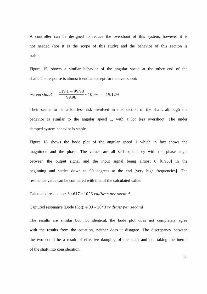
95

A controller can be designed to reduce the overshoot of this system, however it is

not needed (nor it is the scope of this study) and the behavior of this section is

stable.

Figure 15, shows a similar behavior of the angular speed at the other end of the

shaft. The response is almost identical except for the over shoot:

%𝑜𝑣𝑒𝑟𝑠ℎ𝑜𝑜𝑡 =119.1 − 99.98

99.98∗ 100% = 19.12%

Their seems to be a lot less risk involved in this section of the shaft, although the

behavior is similar to the angular speed 1, with a lot less overshoot. The under

damped system behavior is stable.

Figure 16 shows the bode plot of the angular speed 1 which in fact shows the

magnitude and the phase. The values are all self-explanatory with the phase angle

between the output signal and the input signal being almost 0 [0.938] in the

beginning and settles down to 90 degrees at the end [very high frequencies]. The

resonance value can be compared with that of the calculated value:

Calculated resonance: 3.4647 ∗ 10^3 𝑟𝑎𝑑𝑖𝑎𝑛𝑠 𝑝𝑒𝑟 𝑠𝑒𝑐𝑜𝑛𝑑

Captured resonance (Bode Plot): 4.03 ∗ 10^3 𝑟𝑎𝑑𝑖𝑎𝑛𝑠 𝑝𝑒𝑟 𝑠𝑒𝑐𝑜𝑛𝑑

The results are similar but not identical, the bode plot does not completely agree

with the results from the equation, neither does it disagree. The discrepancy between

the two could be a result of effective damping of the shaft and not taking the inertia

of the shaft into consideration.

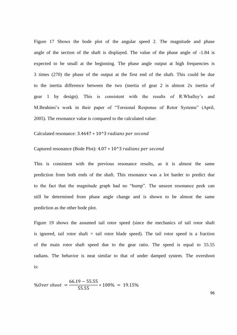
96

Figure 17 Shows the bode plot of the angular speed 2. The magnitude and phase

angle of the section of the shaft is displayed. The value of the phase angle of -1.84 is

expected to be small at the beginning. The phase angle output at high frequencies is

3 times (270) the phase of the output at the first end of the shaft. This could be due

to the inertia difference between the two (inertia of gear 2 is almost 2x inertia of

gear 1 by design). This is consistent with the results of R.Whalley’s and

M.Ibrahimi’s work in their paper of “Torsional Response of Rotor Systems” (April,

2005). The resonance value is compared to the calculated value:



This is consistent with the previous resonance results, as it is almost the same

prediction from both ends of the shaft. This resonance was a lot harder to predict due

to the fact that the magnitude graph had no “hump”. The unseen resonance peek can

still be determined from phase angle change and is shown to be almost the same

prediction as the other bode plot.

Figure 19 shows the assumed tail rotor speed (since the mechanics of tail rotor shaft

is ignored, tail rotor shaft = tail rotor blade speed). The tail rotor speed is a fraction

of the main rotor shaft speed due to the gear ratio. The speed is equal to 55.55

radians. The behavior is neat similar to that of under damped system. The overshoot

is:

%𝑂𝑣𝑒𝑟 𝑠ℎ𝑜𝑜𝑡 =66.19 − 55.55

55.55∗ 100% = 19.15%

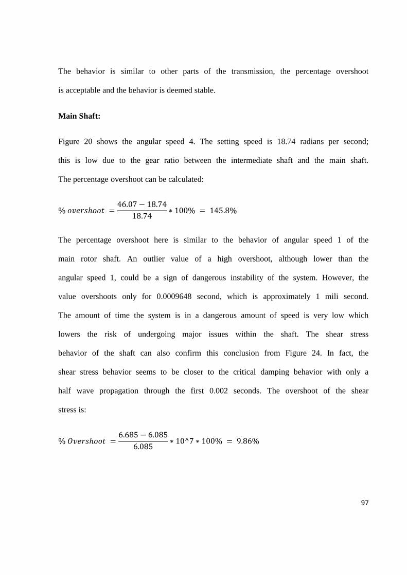
97

The behavior is similar to other parts of the transmission, the percentage overshoot

is acceptable and the behavior is deemed stable.

Main Shaft:

Figure 20 shows the angular speed 4. The setting speed is 18.74 radians per second;

this is low due to the gear ratio between the intermediate shaft and the main shaft.

The percentage overshoot can be calculated:

% 𝑜𝑣𝑒𝑟𝑠ℎ𝑜𝑜𝑡 =46.07 − 18.74

18.74∗ 100% = 145.8%

The percentage overshoot here is similar to the behavior of angular speed 1 of the

main rotor shaft. An outlier value of a high overshoot, although lower than the

angular speed 1, could be a sign of dangerous instability of the system. However, the

value overshoots only for 0.0009648 second, which is approximately 1 mili second.

The amount of time the system is in a dangerous amount of speed is very low which

lowers the risk of undergoing major issues within the shaft. The shear stress

behavior of the shaft can also confirm this conclusion from Figure 24. In fact, the

shear stress behavior seems to be closer to the critical damping behavior with only a

half wave propagation through the first 0.002 seconds. The overshoot of the shear

stress is:

% 𝑂𝑣𝑒𝑟𝑠ℎ𝑜𝑜𝑡 =6.685 − 6.085

6.085∗ 10^7 ∗ 100% = 9.86%

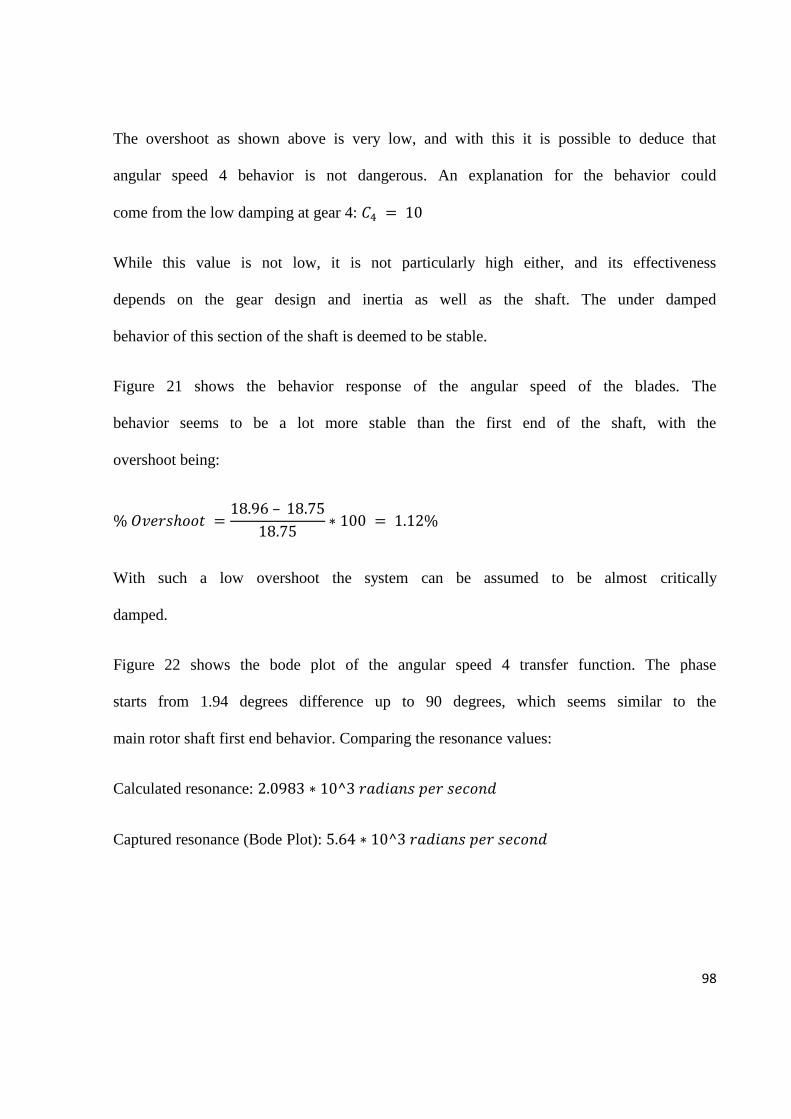
98

The overshoot as shown above is very low, and with this it is possible to deduce that

angular speed 4 behavior is not dangerous. An explanation for the behavior could

come from the low damping at gear 4: 𝐶4 = 10

While this value is not low, it is not particularly high either, and its effectiveness

depends on the gear design and inertia as well as the shaft. The under damped

behavior of this section of the shaft is deemed to be stable.

Figure 21 shows the behavior response of the angular speed of the blades. The

behavior seems to be a lot more stable than the first end of the shaft, with the

overshoot being:

% 𝑂𝑣𝑒𝑟𝑠ℎ𝑜𝑜𝑡 =18.96 – 18.75

18.75∗ 100 = 1.12%

With such a low overshoot the system can be assumed to be almost critically

damped.

Figure 22 shows the bode plot of the angular speed 4 transfer function. The phase

starts from 1.94 degrees difference up to 90 degrees, which seems similar to the

main rotor shaft first end behavior. Comparing the resonance values:



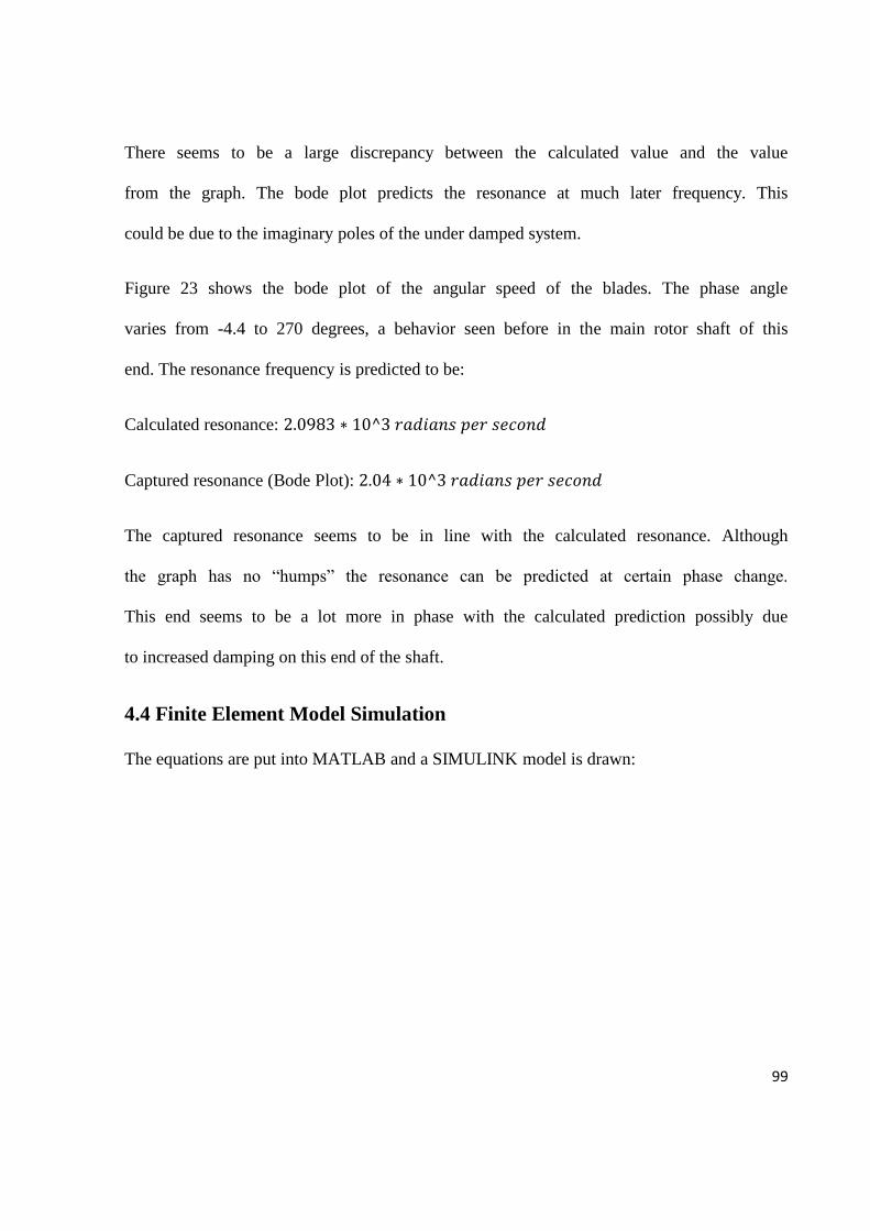
99

There seems to be a large discrepancy between the calculated value and the value

from the graph. The bode plot predicts the resonance at much later frequency. This

could be due to the imaginary poles of the under damped system.

Figure 23 shows the bode plot of the angular speed of the blades. The phase angle

varies from -4.4 to 270 degrees, a behavior seen before in the main rotor shaft of this

end. The resonance frequency is predicted to be:



The captured resonance seems to be in line with the calculated resonance. Although

the graph has no “humps” the resonance can be predicted at certain phase change.

This end seems to be a lot more in phase with the calculated prediction possibly due

to increased damping on this end of the shaft.

4.4 Finite Element Model Simulation

The equations are put into MATLAB and a SIMULINK model is drawn:

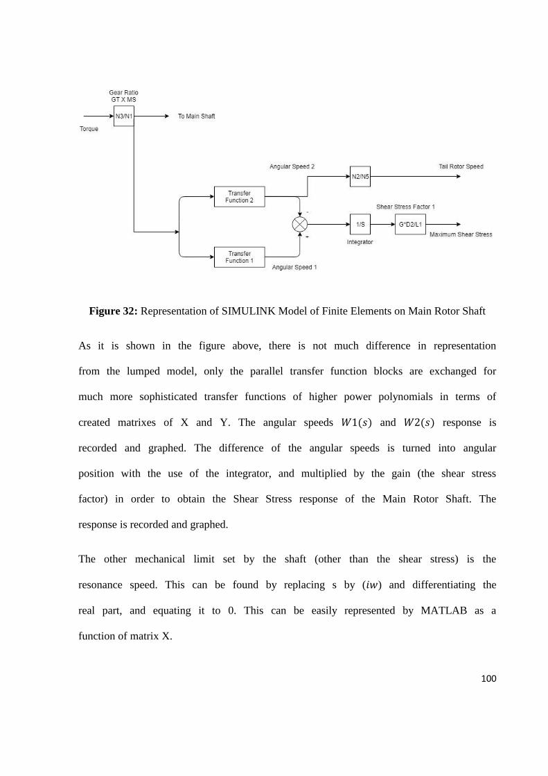
100

Figure 32: Representation of SIMULINK Model of Finite Elements on Main Rotor Shaft

As it is shown in the figure above, there is not much difference in representation

from the lumped model, only the parallel transfer function blocks are exchanged for

much more sophisticated transfer functions of higher power polynomials in terms of

created matrixes of X and Y. The angular speeds 𝑊1(𝑠) and 𝑊2(𝑠) response is

recorded and graphed. The difference of the angular speeds is turned into angular

position with the use of the integrator, and multiplied by the gain (the shear stress

factor) in order to obtain the Shear Stress response of the Main Rotor Shaft. The

response is recorded and graphed.

The other mechanical limit set by the shaft (other than the shear stress) is the

resonance speed. This can be found by replacing s by (𝑖𝑤) and differentiating the

real part, and equating it to 0. This can be easily represented by MATLAB as a

function of matrix X.

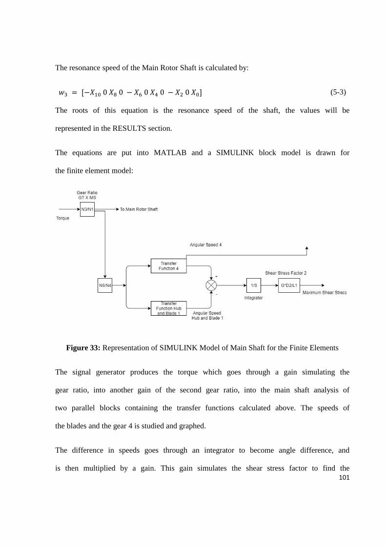
101

The resonance speed of the Main Rotor Shaft is calculated by:

𝑤3 = [−𝑋10 0 𝑋8 0 − 𝑋6 0 𝑋4 0 − 𝑋2 0 𝑋0] (5-3)

The roots of this equation is the resonance speed of the shaft, the values will be

represented in the RESULTS section.

The equations are put into MATLAB and a SIMULINK block model is drawn for

the finite element model:

Figure 33: Representation of SIMULINK Model of Main Shaft for the Finite Elements

The signal generator produces the torque which goes through a gain simulating the

gear ratio, into another gain of the second gear ratio, into the main shaft analysis of

two parallel blocks containing the transfer functions calculated above. The speeds of

the blades and the gear 4 is studied and graphed.

The difference in speeds goes through an integrator to become angle difference, and

is then multiplied by a gain. This gain simulates the shear stress factor to find the

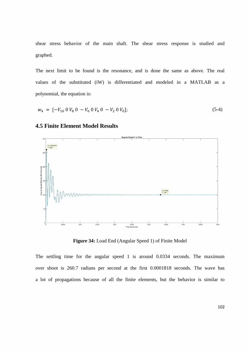
102

shear stress behavior of the main shaft. The shear stress response is studied and

graphed.

The next limit to be found is the resonance, and is done the same as above. The real

values of the substituted (iW) is differentiated and modeled in a MATLAB as a

polynomial, the equation is:

𝑤4 = [−𝑉10 0 𝑉8 0 − 𝑉6 0 𝑉4 0 − 𝑉2 0 𝑉0]; (5-4)

4.5 Finite Element Model Results

Figure 34: Load End (Angular Speed 1) of Finite Model



a lot of propagations because of all the finite elements, but the behavior is similar to

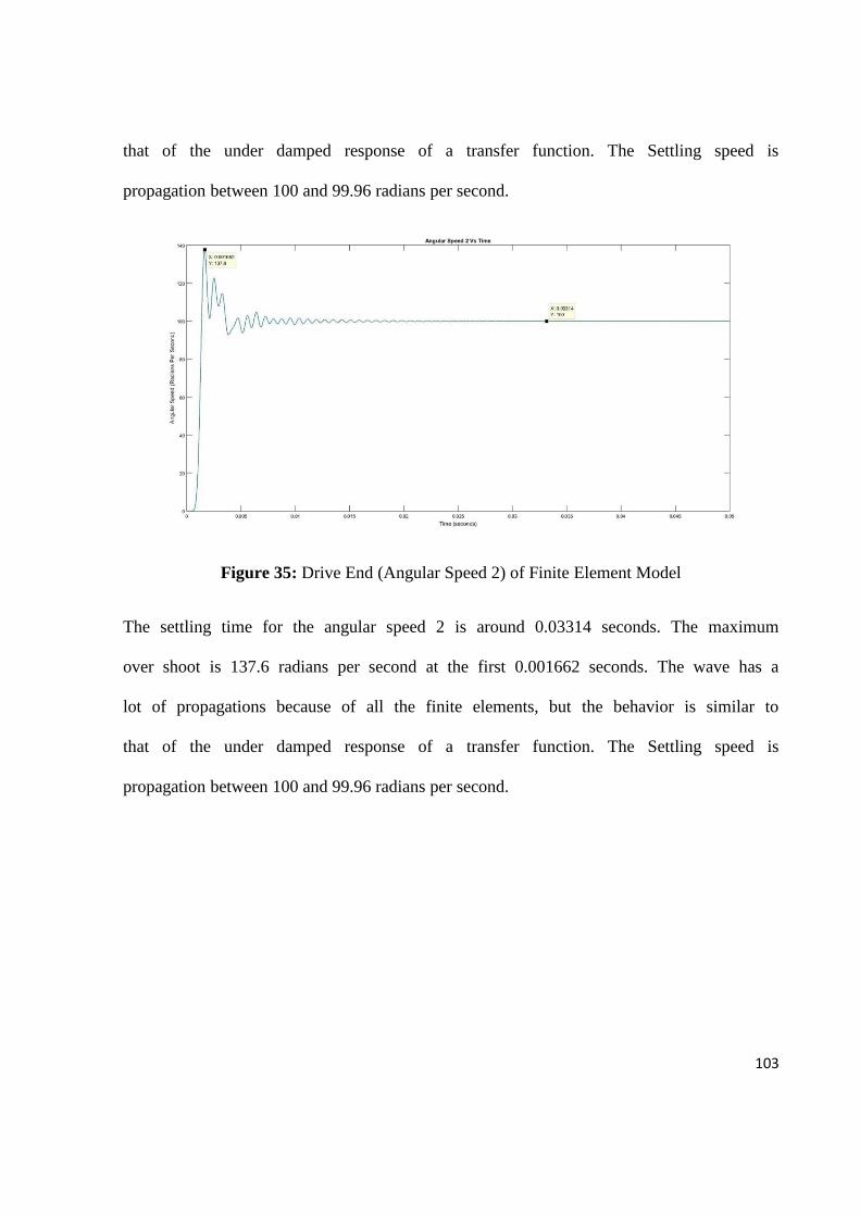
103

that of the under damped response of a transfer function. The Settling speed is

propagation between 100 and 99.96 radians per second.

Figure 35: Drive End (Angular Speed 2) of Finite Element Model


over shoot is 137.6 radians per second at the first 0.001662 seconds. The wave has a

lot of propagations because of all the finite elements, but the behavior is similar to


propagation between 100 and 99.96 radians per second.

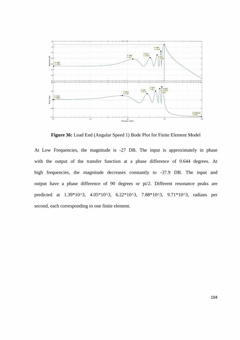
104

Figure 36: Load End (Angular Speed 1) Bode Plot for Finite Element Model

At Low Frequencies, the magnitude is -27 DB. The input is approximately in phase

with the output of the transfer function at a phase difference of 0.644 degrees. At

high frequencies, the magnitude decreases constantly to -37.9 DB. The input and

output have a phase difference of 90 degrees or pi/2. Different resonance peaks are

predicted at 1.39*10^3, 4.05*10^3, 6.22*10^3, 7.88*10^3, 9.71*10^3, radians per

second, each corresponding to one finite element.

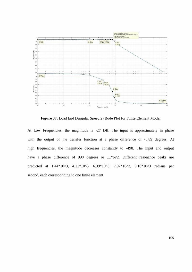
105

Figure 37: Load End (Angular Speed 2) Bode Plot for Finite Element Model

At Low Frequencies, the magnitude is -27 DB. The input is approximately in phase

with the output of the transfer function at a phase difference of -0.89 degrees. At

high frequencies, the magnitude decreases constantly to -498. The input and output

have a phase difference of 990 degrees or 11*pi/2. Different resonance peaks are

predicted at 1.44*10^3, 4.11*10^3, 6.39*10^3, 7.97*10^3, 9.18*10^3 radians per


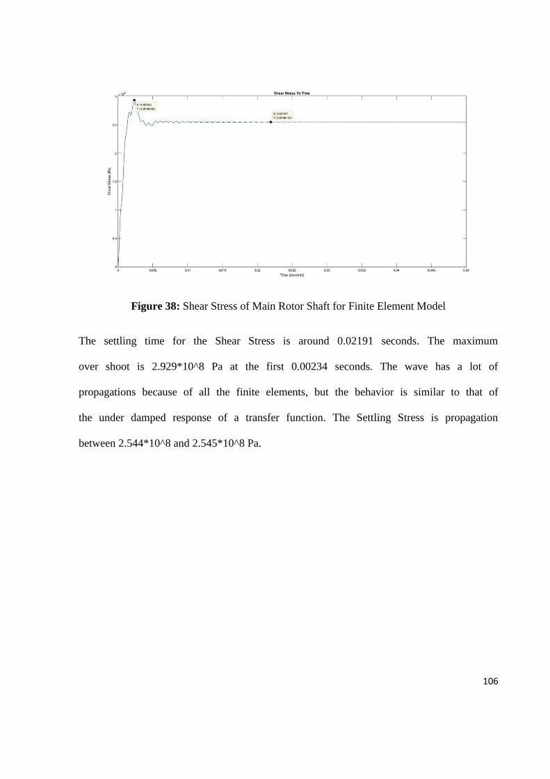
106

Figure 38: Shear Stress of Main Rotor Shaft for Finite Element Model


over shoot is 2.929*10^8 Pa at the first 0.00234 seconds. The wave has a lot of

propagations because of all the finite elements, but the behavior is similar to that of

the under damped response of a transfer function. The Settling Stress is propagation

between 2.544*10^8 and 2.545*10^8 Pa.

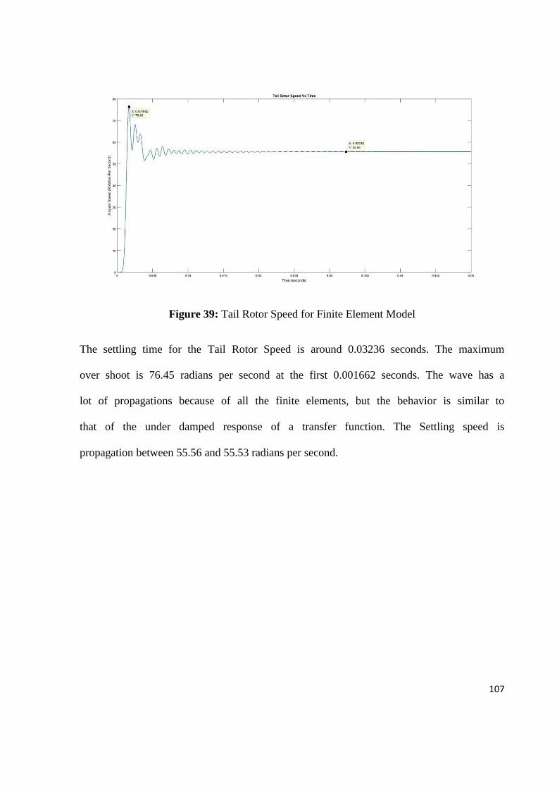
107

Figure 39: Tail Rotor Speed for Finite Element Model

The settling time for the Tail Rotor Speed is around 0.03236 seconds. The maximum


lot of propagations because of all the finite elements, but the behavior is similar to


propagation between 55.56 and 55.53 radians per second.

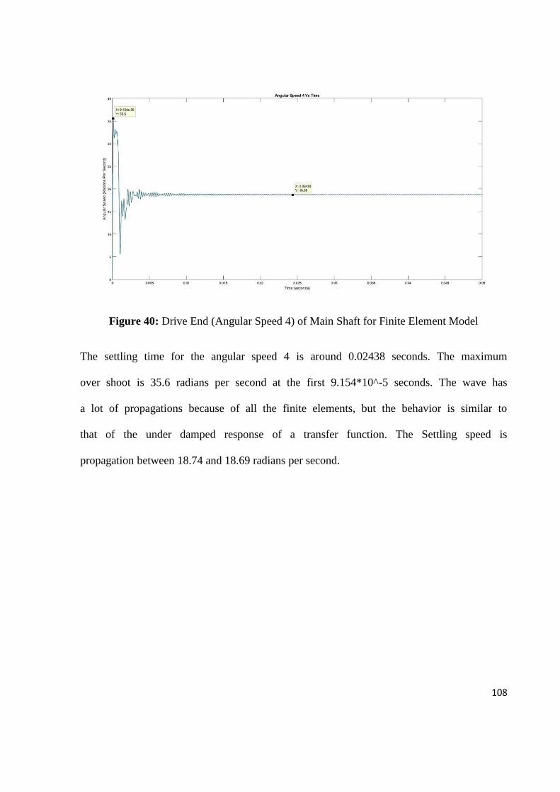
108

Figure 40: Drive End (Angular Speed 4) of Main Shaft for Finite Element Model


over shoot is 35.6 radians per second at the first 9.154*10^-5 seconds. The wave has

a lot of propagations because of all the finite elements, but the behavior is similar to


propagation between 18.74 and 18.69 radians per second.

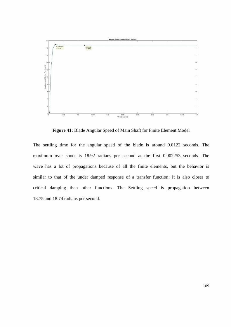
109

Figure 41: Blade Angular Speed of Main Shaft for Finite Element Model

The settling time for the angular speed of the blade is around 0.0122 seconds. The


wave has a lot of propagations because of all the finite elements, but the behavior is

similar to that of the under damped response of a transfer function; it is also closer to

critical damping than other functions. The Settling speed is propagation between

18.75 and 18.74 radians per second.

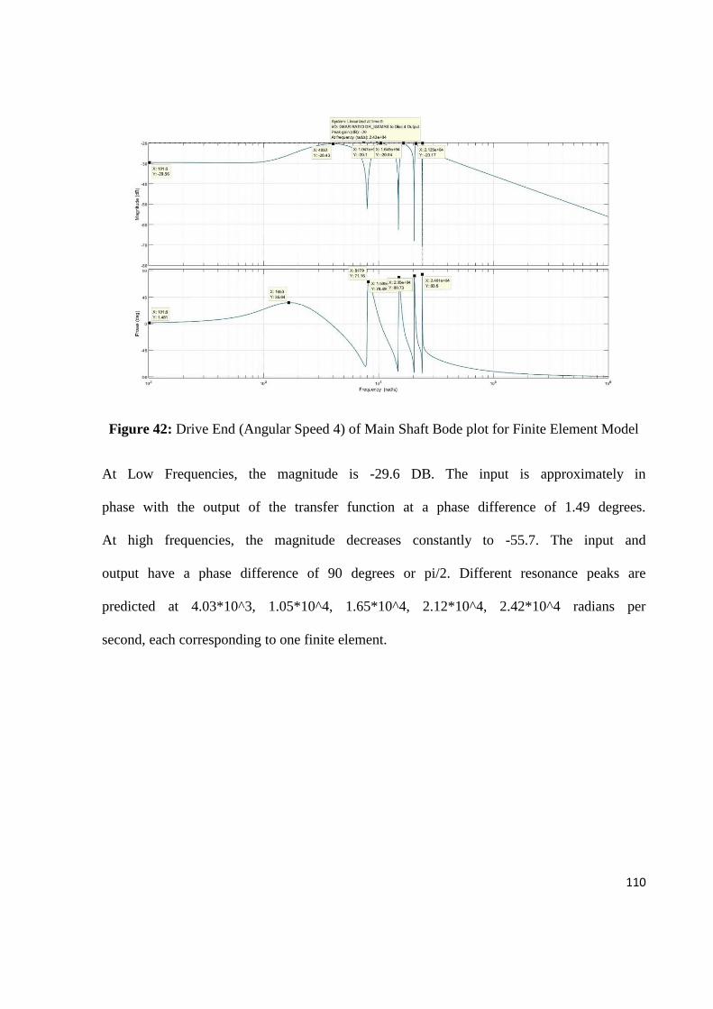
110

Figure 42: Drive End (Angular Speed 4) of Main Shaft Bode plot for Finite Element Model


phase with the output of the transfer function at a phase difference of 1.49 degrees.

At high frequencies, the magnitude decreases constantly to -55.7. The input and

output have a phase difference of 90 degrees or pi/2. Different resonance peaks are

predicted at 4.03*10^3, 1.05*10^4, 1.65*10^4, 2.12*10^4, 2.42*10^4 radians per


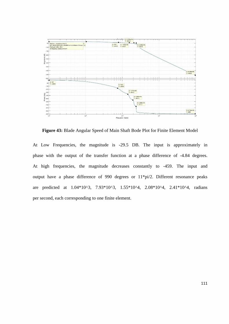
111

Figure 43: Blade Angular Speed of Main Shaft Bode Plot for Finite Element Model


phase with the output of the transfer function at a phase difference of -4.84 degrees.

At high frequencies, the magnitude decreases constantly to -459. The input and

output have a phase difference of 990 degrees or 11*pi/2. Different resonance peaks

are predicted at 1.04*10^3, 7.93*10^3, 1.55*10^4, 2.08*10^4, 2.41*10^4, radians

per second, each corresponding to one finite element.

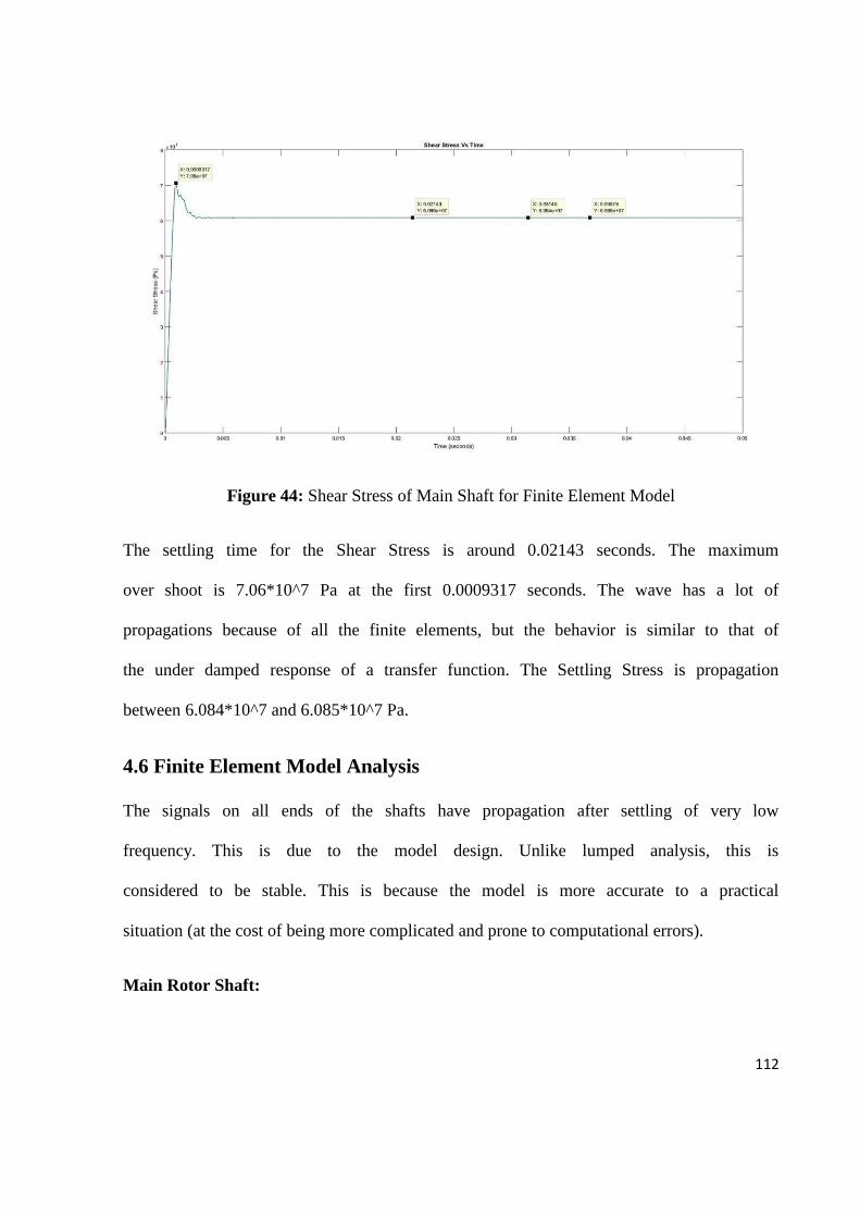
112

Figure 44: Shear Stress of Main Shaft for Finite Element Model


over shoot is 7.06*10^7 Pa at the first 0.0009317 seconds. The wave has a lot of

propagations because of all the finite elements, but the behavior is similar to that of

the under damped response of a transfer function. The Settling Stress is propagation

between 6.084*10^7 and 6.085*10^7 Pa.

4.6 Finite Element Model Analysis

The signals on all ends of the shafts have propagation after settling of very low

frequency. This is due to the model design. Unlike lumped analysis, this is

considered to be stable. This is because the model is more accurate to a practical

situation (at the cost of being more complicated and prone to computational errors).

Main Rotor Shaft:

113

Figure 25 shows the response of the angular speed 1. Mind the propagations of the

wave, the overall shape of the signal is similar to the under damped behavior. These

propagations are due to the shaft being distributed into 5 elements. Similarly, to the

lumped model, the overshoot is calculated:

% 𝑜𝑣𝑒𝑟 𝑠ℎ𝑜𝑜𝑡 =260.7 − 100

100∗ 100% = 160.7%

This is similar to the lumped model, except the overshoot now is almost half of what

is predicted before. This is not considered unhealthy as it only stays for the first 0.18

milliseconds of the response. The transfer function of the first end is still considered

to be under damped.

Figure 26 shows the response behavior of angular speed 2. Comparing the finite

model to the lumped model, the speed seems to settle a lot later than the lumped

model (from 0.005 seconds to 0.03 seconds), however, since the time itself is very

short, this is not an issue at all. The overshoot is calculated to be:

% 𝑜𝑣𝑒𝑟 𝑠ℎ𝑜𝑜𝑡 =137.6 − 100

100∗ 100% = 37.6%

The overshoot seems to be a little bit higher than the lumped model; this means that

a lot more vibrations should be expected in this section of the shaft. To get a better

conclusion the shear stress behavior is observed.

Figure 29 shows the shear stress behavior of the main rotor shaft. This response is

approximately identical to that of the lumped model, mind the propagations caused

by the finite elements model. The over shoot of this is calculated:

114

% 𝑂𝑣𝑒𝑟𝑠ℎ𝑜𝑜𝑡 =2.929 − 2.544

2.544∗ 100% = 45.29%

Although the behavior is the same, the overshoot is twice as high; this explains the

higher overshoot at the gear 2 end of the shaft. However, it is concluded that the

system is not in danger of approaching instability, due to the short time to reach the

overshoot, and the overall behavior of the speed and stress signals.

Figure 30 shows the tail rotor speed. This speed is predicted to be similar to the

angular speed 2, but only a fraction of it in value as of the gear ratio between them.

The over shoot is:

% 𝑂𝑣𝑒𝑟𝑠ℎ𝑜𝑜𝑡 =76.45 – 55.56

55.56∗ 100% = 37.59%

The over shoot behavior is also similar and occurs only during the first 0.001662

seconds and is not considered to be an issue to the stability of the system.

Figure 27 shows the bode plot of angular speed 1 transfer function. There seems to

be a lot of propagations compared the lumped model analysis. In fact it’s assumed to

be one real resonance peak for each finite element. The resonance values are:

Calculated resonance: 1.0 ∗ 10^3 ∗ (9.2826, 7.8770, 6.2746, 4.0327, 1.3900)

Captured resonance (Bode Plot): 1.39 ∗ 10^3, 4.05 ∗ 10^3, 6.22 ∗ 10^3, 7.88 ∗

10^3, 9.71 ∗ 10^3

115

The values from the graph seem to be in line with the calculated values, which

seems to conclude that this method is a lot more accurate than the lumped model

analysis, with increased consistency.

Figure 28 shows the bode plot of angular speed 2. The graph seems a lot harder to

read than angular speed 1 perhaps due to damping. This is consistent with the

lumped model on the other hand. The resonance values are found to be:



10^3, 9.18 ∗ 10^3

Although the values appear to have a little higher discrepancy, they are still very

consistent with both calculated results, and the bode results from the other end of the

shaft.

Main Shaft:

Figure 31 shows the angular speed 4 behavior response. The shape of the signal

indicates this is an under damped response with the over shoot to be:

% 𝑂𝑣𝑒𝑟𝑠ℎ𝑜𝑜𝑡 =35.6 − 18.74

18.74∗ 100 = 89.97%

As expected the overshoot is higher on the first end of the shaft. This was also seen

in the lumped model analysis. For a conclusion to be made, the time and stress must

be looked at.

116

Figure 35 shows the shear stress in the main shaft. The response seems to be close to

that of a critical damped system. The overshoot is:

% 𝑂𝑣𝑒𝑟 𝑠ℎ𝑜𝑜𝑡 =7.06 − 6.084

6.084∗ 100% = 16.04%

The over shoot seems to be very low. Even though this is the finite element model

analysis there are a lot less propagations than expected, this is a hint towards the

system’s stability. The time it takes for the angular speed 4 to reach the overshoot is

0.02438 seconds. These two low values excel at concluding that the high overshoot

is not of large concern towards system stability.

Figure 32 shows the speed of the blade end. The behavior of the response is a sign

that shows that the transfer function of this speed is almost critically damped. The

over shoot is calculated to be:

% 𝑂𝑣𝑒𝑟𝑠ℎ𝑜𝑜𝑡 =18.92 − 18.75

18.75∗ 100% = 0.91%

This value is agreeable of the analysis of the lumped model and this section is

considered to be stable.

Figure 33 shows the bode plot of angular speed 4. Similarly to the main rotor shaft,

there are 5 peaks considered to hold the frequency for resonance speed, because of

the 5 finite element modeling. The resonance frequency is compared:


117


10^4, 2.42 ∗ 10^4

As seem from the comparison of the values, the first two resonance frequencies have

a large discrepancy while the last three values are similar. This seems to be

consistent what was found from the lumped analysis and might be a damping issue.

However this is but a prediction and is not enough to dismiss it as instability,

although it is not entirely out of concern.

Figure 34 shows the bode plot of the blade transfer function. The peaks are hard to

read as seen in the lumped model but still can be deduced from the phase change and

be used for comparison between:



10^4, 2.41 ∗ 10^4

These values are much more in line with the calculated values and approved for

consistency and precision.

4.7 Hybrid (Distributed-Lumped) Model Simulation

Putting the necessary equations in MATLAB in order to produce the following

simulation in SIMULINK:

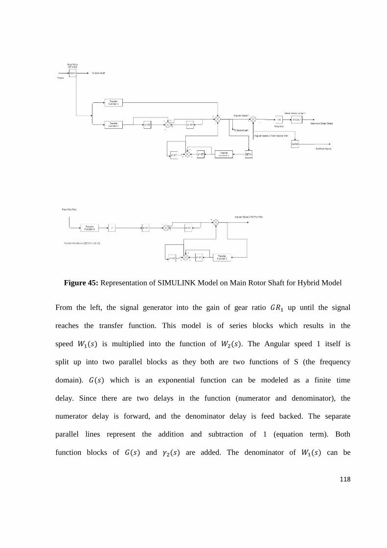
118

Figure 45: Representation of SIMULINK Model on Main Rotor Shaft for Hybrid Model

From the left, the signal generator into the gain of gear ratio 𝐺𝑅1 up until the signal

reaches the transfer function. This model is of series blocks which results in the

speed 𝑊1(𝑠) is multiplied into the function of 𝑊2(𝑠). The Angular speed 1 itself is

split up into two parallel blocks as they both are two functions of S (the frequency

domain). 𝐺(𝑠) which is an exponential function can be modeled as a finite time

delay. Since there are two delays in the function (numerator and denominator), the

numerator delay is forward, and the denominator delay is feed backed. The separate

parallel lines represent the addition and subtraction of 1 (equation term). Both

function blocks of 𝐺(𝑠) and 𝛾2(𝑠) are added. The denominator of 𝑊1(𝑠) can be

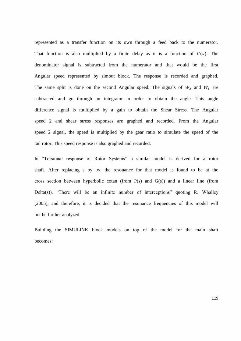
119

represented as a transfer function on its own through a feed back to the numerator.

That function is also multiplied by a finite delay as it is a function of 𝐺(𝑠). The

denominator signal is subtracted from the numerator and that would be the first

Angular speed represented by simout block. The response is recorded and graphed.

The same split is done on the second Angular speed. The signals of 𝑊2 and 𝑊1 are

subtracted and go through an integrator in order to obtain the angle. This angle

difference signal is multiplied by a gain to obtain the Shear Stress. The Angular

speed 2 and shear stress responses are graphed and recorded. From the Angular

speed 2 signal, the speed is multiplied by the gear ratio to simulate the speed of the

tail rotor. This speed response is also graphed and recorded.

In “Torsional response of Rotor Systems” a similar model is derived for a rotor

shaft. After replacing s by iw, the resonance for that model is found to be at the

cross section between hyperbolic cotan (from P(s) and G(s)) and a linear line (from

Delta(s)). “There will be an infinite number of interceptions” quoting R. Whalley

(2005), and therefore, it is decided that the resonance frequencies of this model will

not be further analyzed.

Building the SIMULINK block models on top of the model for the main shaft

becomes:

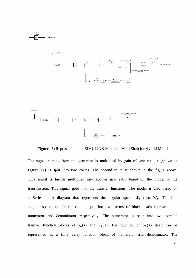
120

Figure 46: Representation of SIMULINK Model on Main Shaft for Hybrid Model

The signal coming from the generator is multiplied by gain of gear ratio 1 (shown in

Figure 12) is split into two routes. The second route is shown in the figure above.

This signal is further multiplied into another gear ratio based on the model of the

transmission. This signal goes into the transfer functions. The model is also based on

a Series block diagram that represents the angular speed 𝑊1 then 𝑊2. The first

angular speed transfer function is split into two terms of blocks each represents the

numerator and denominator respectively. The numerator is split into two parallel

transfer function blocks of 𝛾4(𝑠) and 𝐺2(𝑠). The function of 𝐺2(𝑠) itself can be

represented as a time delay function block of numerator and denominator. The

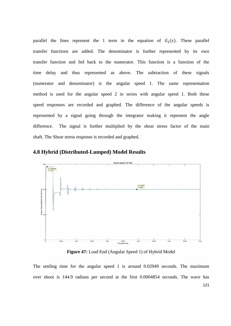
121

parallel the lines represent the 1 term in the equation of 𝐺2(𝑠). These parallel

transfer functions are added. The denominator is further represented by its own

transfer function and fed back to the numerator. This function is a function of the

time delay and thus represented as above. The subtraction of these signals

(numerator and denominator) is the angular speed 1. The same representation

method is used for the angular speed 2 in series with angular speed 1. Both these

speed responses are recorded and graphed. The difference of the angular speeds is

represented by a signal going through the integrator making it represent the angle

difference. The signal is further multiplied by the shear stress factor of the main

shaft. The Shear stress response is recorded and graphed.

4.8 Hybrid (Distributed-Lumped) Model Results

Figure 47: Load End (Angular Speed 1) of Hybrid Model



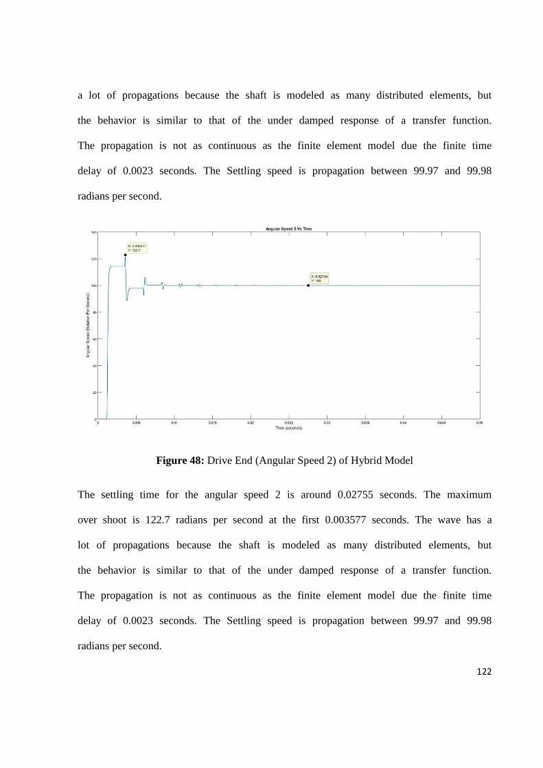
122

a lot of propagations because the shaft is modeled as many distributed elements, but

the behavior is similar to that of the under damped response of a transfer function.

The propagation is not as continuous as the finite element model due the finite time

delay of 0.0023 seconds. The Settling speed is propagation between 99.97 and 99.98

radians per second.

Figure 48: Drive End (Angular Speed 2) of Hybrid Model



lot of propagations because the shaft is modeled as many distributed elements, but



delay of 0.0023 seconds. The Settling speed is propagation between 99.97 and 99.98

radians per second.

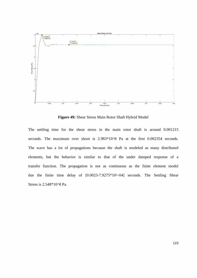
123

Figure 49: Shear Stress Main Rotor Shaft Hybrid Model

The settling time for the shear stress in the main rotor shaft is around 0.001215

seconds. The maximum over shoot is 2.983*10^8 Pa at the first 0.002354 seconds.

The wave has a lot of propagations because the shaft is modeled as many distributed

elements, but the behavior is similar to that of the under damped response of a

transfer function. The propagation is not as continuous as the finite element model

due the finite time delay of [0.0023-7.9275*10^-04] seconds. The Settling Shear

Stress is 2.548*10^8 Pa.

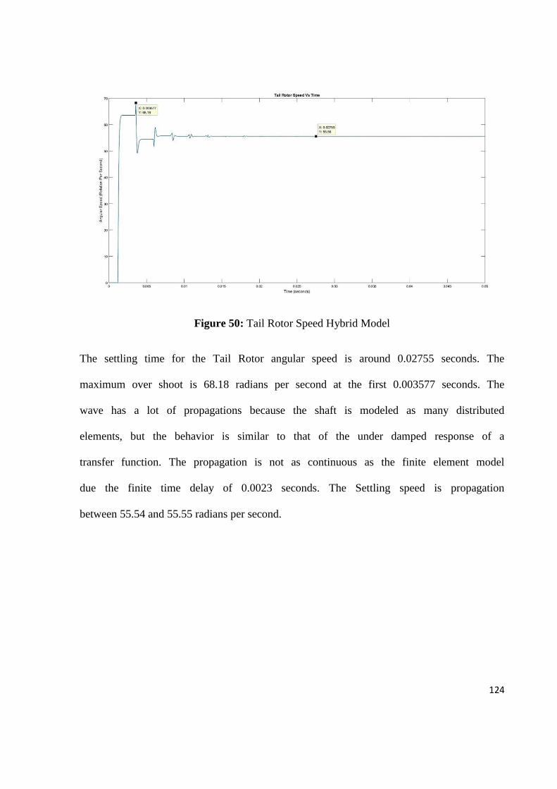
124

Figure 50: Tail Rotor Speed Hybrid Model

The settling time for the Tail Rotor angular speed is around 0.02755 seconds. The


wave has a lot of propagations because the shaft is modeled as many distributed



due the finite time delay of 0.0023 seconds. The Settling speed is propagation

between 55.54 and 55.55 radians per second.

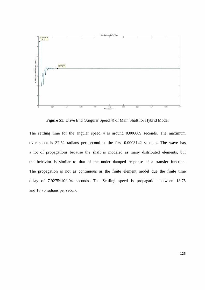
125

Figure 51: Drive End (Angular Speed 4) of Main Shaft for Hybrid Model



a lot of propagations because the shaft is modeled as many distributed elements, but



delay of 7.9275*10^-04 seconds. The Settling speed is propagation between 18.75

and 18.76 radians per second.

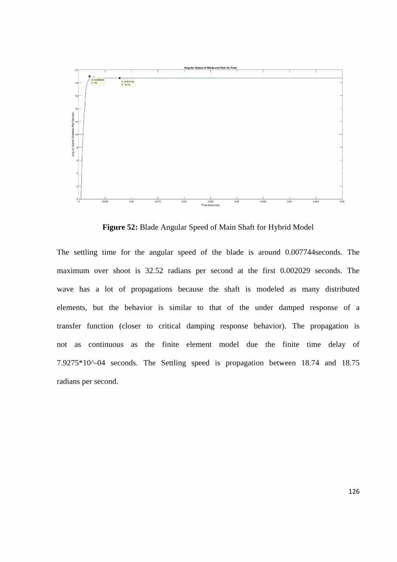
126

Figure 52: Blade Angular Speed of Main Shaft for Hybrid Model

The settling time for the angular speed of the blade is around 0.007744seconds. The




transfer function (closer to critical damping response behavior). The propagation is

not as continuous as the finite element model due the finite time delay of

7.9275*10^-04 seconds. The Settling speed is propagation between 18.74 and 18.75

radians per second.

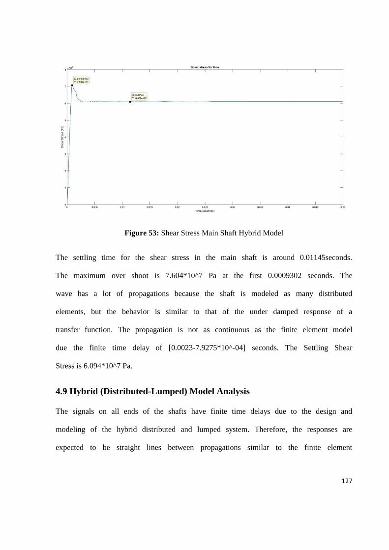
127

Figure 53: Shear Stress Main Shaft Hybrid Model

The settling time for the shear stress in the main shaft is around 0.01145seconds.

The maximum over shoot is 7.604*10^7 Pa at the first 0.0009302 seconds. The




due the finite time delay of [0.0023-7.9275*10^-04] seconds. The Settling Shear

Stress is 6.094*10^7 Pa.

4.9 Hybrid (Distributed-Lumped) Model Analysis

The signals on all ends of the shafts have finite time delays due to the design and

modeling of the hybrid distributed and lumped system. Therefore, the responses are

expected to be straight lines between propagations similar to the finite element

128

analysis but less severe and continuous. This model is most accurate for long shaft

lengths.

Main Rotor Shaft:

Figure 36 shows the response of the angular speed 1. As expected the behavior is

propagations with straight lines showing the effect of finite time delays. The

behavior is still that of an under damped system, and the over shoot is found to be:

% 𝑂𝑣𝑒𝑟𝑠ℎ𝑜𝑜𝑡 =144.9 − 99.98

99.98∗ 100% = 44.92%

Out of all models, this model gives off the least amount of overshoot for this

particular speed and is because of the effect of the finite time delay (cuts the signal

behavior until after the time delay where it starts to decrease).

Figure 37 shows the behavior of angular speed 2. Unlike angular speed 1 this

response starts with a delay due the function block of the SIMULINK modeling, in

other words, the nature of the transfer function. The over shoot of the system is

effected by this:

% 𝑂𝑣𝑒𝑟 𝑠ℎ𝑜𝑜𝑡 =122.7 − 99.98

99.98∗ 100% = 22.72%

Although the overshoot of angular speed 1 is greatly affected by the time delay

compared to other models, the overshoot for angular speed 2 does not seem to be

that much affected. This is because it starts with the time delay 0.0023 which is

smaller than the rise time (to reach the overshoot) which is 0.02755 seconds.

129

Figure 38 shows the shear stress behavior along the main rotor shaft. The shear

stress does not seem very different in all models of study. However, it still possible

to see the small effects of the time delays in the difference of angular speeds (1 and

2). The overshoot is:

% 𝑂𝑣𝑒𝑟𝑠ℎ𝑜𝑜𝑡 =2.983 − 2.548

2.548∗ 100% = 17.07%

The overshoot behavior is also similar to other models.

Figure 30 shows the tail rotor speed response. Like other models this model is

exactly similar to the angular speed 2 model but with a difference in settling speed

due to the gear ratio. The over shoot can still be calculated to be:

% 𝑂𝑣𝑒𝑟 𝑠ℎ𝑜𝑜𝑡 =68.18 − 55.55

55.55∗ 100% = 22.73%

Figure 40 shows the behavior of the angular speed 4. The response is similar to the

finite element model due to the small time constant of the finite time delay

(7.9275*10^-04 seconds). The over shoot of the signal is:

% 𝑂𝑣𝑒𝑟𝑠ℎ𝑜𝑜𝑡 =32.52 − 18.76

18.76∗ 100% = 73.33%

The over shoot is still high as the other models have also shown but due to the shear

stress behavior shown next and a small rise time of 0.3 mili seconds, this behavior is

accepted.

130

Figure 42 shows the shear stress along the main shaft. The response shows similar

characteristics of previous models to due to very small finite time delay difference.

The overshoot becomes:

% 𝑂𝑣𝑒𝑟 𝑠ℎ𝑜𝑜𝑡 =7.604 − 6.094

6.094∗ 100% = 24.78%

Just as the other models have predicted the over shoot is small and in an acceptable

range, making the over shoot in angular speed 4 also acceptable.

Figure 41 shows the angular speed of the blades. The finite time delay effect can be

seen in forms of stagnation between small propagations. The system response here is

still close to critical damping as other models have shown. The over shoot is:

% 𝑂𝑣𝑒𝑟𝑠ℎ𝑜𝑜𝑡 =32.52 − 18.75

18.75∗ 100% = 1.33%

The small overshoot corresponds to an almost critically damped system, and the

speed is deemed to be stable.

131

Chapter V: Conclusions & Recommendations

This section explains the behavior of the corresponding response, based on analysis,

model, and actual behavior of the shafts, gears and blades. The respective results are

referenced from their figure number.

To summarize, the three modeling techniques for rotor drive line system were

derived. The mathematical equations were extracted as ordinary differential

equations from the lumped and finite element model, and as partial differential

equations in the hybrid (transmission line) model. The transmission of the helicopter

was designed element by element, including shafts, gears, dampers, hubs and blades.

Using both, the mathematical model and element design a simulation has been run

on the system to find the output response. This response is in terms of angular

velocity and torsional shear stress. The lumped model was a more direct approach to

the theoretical derivation of the drive line system. The response was smooth for the

most part; with a small exception regarding the overshoots. However, this was

observed in all of the models, making it more of a design flaw than a modeling flaw.

The lumped model is simple and easy to derive and simulate but less accurate as it is

affected by assumptions and non linarites. The finite element model holds more

complexity in terms of mathematical derivation. This gives the value of the behavior

(of the responses) a lot more weight. However, with more complexity comes more

difficulty in solving the equations, and with more difficulty comes less accuracy.

The more the finite elements the higher the order of the polynomial, the more prone

to making mistakes the designer is. The hybrid model shows closer behavior to that

132

of the finite element, adding more weight to the value of the response found. The

hybrid model weakness is shown from the difficulty of obtaining the resonance or

critical speeds of the shaft. This becomes a nuisance as this information is needed to

prevent mechanical failure.

133

References

2018, Understanding of resonance essential for solving vibration problems | Control

Engineering. [online] Available at: https://www.controleng.com/single-article/understanding-

of-resonance-essential-for-solving-vibration-

problems/d488603700c4d41d9797cece595e8e74.html [Accessed 15 Nov. 2018].

2019, [online] Available at: http://navybmr.com/study%20material/14008a/14008A_ch7.pdf

[Accessed 6 Jan. 2019].

Ameer, A. (2010). Distributed Parameter System Modeling, Lecture 1.



Asmar, N. (2017). Partial Differential Equations with Fourier Series and Boundary Value

Problems. Dover Publications.

Bartlett, H. and Whalley, R. (1998). Analogue solution to the modelling and simulation of

distributed-lumped parameter systems. Proceedings of the Institution of Mechanical

Engineers, Part I: Journal of Systems and Control Engineering, 212(2), pp.99-114.

Bathe K. J. (1976) Numerical methods in finite element analysis, Prentice-Hall

Budynas. (n.d.). Shigleys mechanical engineering design, 9th ed. Mc Graw Hill: 2010.

C. Hibbeler, R. (2015). Engineering Mechanics + Mastering Engineering With Pearson Etext.

14th ed. Pearson College Div.

Cengel, Y., Kanoglu, M. and Boles, M. (2007). Thermodynamics. 6th ed. New York:

McGraw-Hill.

Doebelin, E. (1998). System dynamics. New York: Marcel Dekker.

Dorf, R. and Bishop, R. (2010) Modern Control Systems, 12th Edition, Pearson.

Ebrahimi, M. and Whalley, R. (2000). Analysis, Modeling and Simulation of stiffness in

machine tool drives. Computers & Industrial Engineering, 38(1), pp.93-105.

Fundamentals of Gas Turbine Engines. (n.d.).

Gregersen, E. (2017). Torque | Equation, Definition, & Units. [online] Encyclopedia

Britannica. Available at: https://www.britannica.com/science/torque [Accessed 28 Jun. 2017].

Gunston, B. (2006). The development of jet and turbine aero engines. Sparkford, Somerset:

Patrick Stephens.

134

Helicopter instructor's handbook. (2012). New Castle, Wash.: Aviation Supplies &

Academics, Inc.

Industries, P. (2015). A History of the Helicopter | Prime Industries. [online] Prime Industries.

Available at: https://primeindustriesusa.com/history-of-the-helicopter/ [Accessed 27 Jan.

2019].

Jiang, Y., Yang, Z. and Gao, J. (2011). The Application and Development of the High Speed

Overrunning Clutch in the Transmission System of the Helicopter. Applied Mechanics and

Materials, 86, pp.283-286.

John, S., Mishra, R. and Shetty, B. (2017). Development of Reclamation Technology for a

Turbo-Shaft Engine. Journal of Failure Analysis and Prevention, 17(2), pp.255-261.

Kalkat, M., Yıldırım, Ş. and Uzmay, I. (2003). Rotor Dynamics Analysis of Rotating Machine

Systems Using Artificial Neural Networks. International Journal of Rotating Machinery,

9(4), pp.255-262.

Karakash, J. (1951). Transmission lines and filter networks. Macmillan.

Modeling of Mechanical Vibrations, n.d.

Mohaideen, M. (2012). Optimization and Analysis on Turbine Rotor of a Turbo Shaft

Engine. Procedia Engineering, 38, pp.867-871.

MVR, R. (2015). Aerodynamic Load Estimation of Helicopter Rotor in Hovering

Flight. Journal of Aeronautics & Aerospace Engineering, 05(01).

Padfield, R. (n.d.). Learning to fly helicopters.

Poluiyanin, A. and Zaæiutysev, V. (2003). Handbook of exact solutions for ordinary

differential equations. Boca Raton: Chapman & Hall/CRC.

Seddon, J. and Newman, S. (2011). Basic Helicopter Aerodynamics. Hoboken: Wiley.

Siemens Gas Turbine. (2015). [ebook] Mahmood El Naggar. Available at:

https://www.slideshare.net/manojg1990/236407565-gasturbinenotes [Accessed 6 Jan. 2019].

Slager, A. (2015). Examination of a Helicopter Main Transmission Spiral Bevel Gear

Fractures Due to Intergranular Attack and Fatigue. Journal of Failure Analysis and

Prevention, 15(3), pp.441-444.

Sontag, E. (1998). Mathematical control theory : deterministic finite dimensional systems.

New York: Springer.

Turboshaft Engine. (2019). [ebook] Thirumalvalavan. Available at:

https://www.slideshare.net/manothirumal/turbo-shaft-engine [Accessed 6 Jan. 2019].

Whalley, R. (1990). Interconnected spatially distributed systems. Transactions of the Institute

of Measurement and Control, 12(5), pp.262-270.

135

Whalley, R. (1998). Three-term control of lightly damped mechanical systems. Proceedings

of the Institution of Mechanical Engineers, Part C: Journal of Mechanical Engineering

Science, 212(2), pp.153-164.

Whalley, R. and A-Ameer, A. (2009). The computation of torsional, dynamic

stresses. Proceedings of the Institution of Mechanical Engineers, Part C: Journal of

Mechanical Engineering Science, 223(8), pp.1799-1814.

Whalley, R. and Abdul-Ameer, A. (2009). Contoured shaft and rotor dynamics. Mechanism

and Machine Theory, 44(4), pp.772-783.

Whalley, R. and Ebrahimi, M. (2000). The regulation of mechanical drive systems. Applied

Mathematical Modelling, 24(4), pp.247-262.

Whalley, R., Abdul-Ameer, A. and Ebrahimi, M. (2008). Machine tool modelling and profile

following performance. Applied Mathematical Modelling, 32(11), pp.2290-2311.

Whalley, R., Ebrahimi, M. and Abdul-Ameer, A. (2005). Hybrid modelling of machine tool

axis drives. International Journal of Machine Tools and Manufacture, 45(14), pp.1560-1576.

Whalley, R., Ebrahimi, M. and Abdul-Ameer, A. (2007). High-speed rotor-shaft systems and

whirling identification. Proceedings of the Institution of Mechanical Engineers, Part C:

Journal of Mechanical Engineering Science, 221(6), pp.661-676.

Whalley, R., Ebrahimi, M. and Jamil, Z. (2005). The torsional response of rotor

systems. Proceedings of the Institution of Mechanical Engineers, Part C: Journal of

Mechanical Engineering Science, 219(4), pp.357-380.

White, G. (1998). Design study of a split-torque helicopter transmission. Proceedings of the

Institution of Mechanical Engineers, Part G: Journal of Aerospace Engineering, 212(2),

pp.117-123.

Images:

https://upload.wikimedia.org/wikipedia/commons/thumb/6/69/Turboshaft_operation_%28mul

tilanguage%29.svg/440px-Turboshaft_operation_%28multilanguage%29.svg.png

https://www.faasafety.gov/gslac/ALC/course_content.aspx?cID=105&sID=461&preview=tru

e [Accessed 6 Jan. 2019]

136

Appendix I

MATLAB EQUATIONS:

% All Gears

H = 0.02; %m

D = 7000; %kg/m3

% All Blades

DB = 3000; %kg/m3

% Main Shaft (Tail Rotor,Hollow)

% Inertia of the Shaft:

D1MS = 0.0655; %m

D2MS = 0.07; %m

L1MS = 3.96; %m

I1MS = pi*D*L1MS*(1/32)*((D2MS^4)-(D1MS^4)); %kgm2

% Inertia of the disc 1:

% Number of Teeth = 50

NTD1 = 50;

% Rotation = 2040 rpm

D1D1 = 0.08; %m

D2D1 = 0.10; %m

I1 = pi*D*H*(1/32)*((D2D1^4)-(D1D1^4)); %kgm2



137

NTD2 = 25;


D1D2 = 0.08; %m

D2D2 = 0.115; %m

I2 = pi*D*H*(1/32)*((D2D2^4)-(D1D2^4)); %kgm2

% Gas Turbine Shaft (Not Hollow)

% Power = 350 HP


NTD3 = 40;


% Inertia of the Shaft

D1GTS = 0.1; %m

L1GTS = 0.2; %m

I1GTS = pi*D*L1GTS*(1/32)*(D1GTS^4); %kgm2

% Inertia of the disc 3

D1D3 = 0.03; %m

D2D3 = 0.05; %m

I3 = pi*D*H*(1/32)*((D2D3^4)-(D1D3^4)); %kgm2

% Main Rotor Shaft

% Inertia of the Shaft

D1MRS = 0.042; %m

138

D2MRS = 0.05; %m

L1MRS = 1.34; %m

I1MRS = pi*D*L1MRS*(1/32)*((D2MRS^4)-(D1MRS^4)); %kgm2



NTD4 = 60;


D1D4 = 0.1; %m

D2D4 = 0.11; %m

I4 = pi*D*H*(1/32)*((D2D4^4)-(D1D4^4)); %kgm2

% Inertia of the Blades 1

NB1 = 5;

LB1 = 4.03; %m

D1B1 = 0.02; %m

IB1 = NB1*pi*DB*LB1*(1/32)*(D1B1^4); %kgm2

% Inertia of the Hub 1

DH1 = 0.1; %m

LH1 = 0.35; %m

IH1 = pi*DB*LH1*(1/32)*(DH1^4); %kgm2

% Tail Rotor Shaft

% Inertia of the Shaft = IGNORED because the shaft is too small

% Inertia of the Hub = IGNORED because the mass is too small

139

% Inertia of the blades 2 (Fixed on a small shaft)

NB2 = 4;

LB2 = 0.7; %m

D1B2 = 0.01; %m

I1B2 = NB2*pi*DB*LB2*(1/32)*(D1B2^4); %kgm2



NTD5 = 45;


D1D5 = 0.01; %m

D2D5 = 0.1; %m

I5 = pi*D*H*(1/32)*((D2D5^4)-(D1D5^4)); %kgm2

% Intermediate Shaft

% Inertia of the Shaft = IGNORED because the shaft is too small



NTD6 = 15;


D1D6 = 0.01; %m

D2D6 = 0.1; %m

I6 = pi*D*H*(1/32)*((D2D6^4)-(D1D6^4)); %kgm2

140

% Gear Ratios

% Gas Turbine X Main Shaft

GR_GTXMS = NTD3/NTD1;

% Main Shaft x Tail Rotor Shaft

GR_MSXTRS = NTD2/NTD5;

% Intermediate Shaft x Main Rotor Shaft

GR_ISXMRS = NTD6/NTD4;

% Maximum Shear Stress:

% TAW = Angle*G*R/L

% R = Outer Radius

% L = Length of Shaft

% Substitution:

% K = G*J/L EQUATION

% SSF = G*R/L EQUATION

J1 = I1;

J2 = I2;

J1MS = I1MS;

G = 80*10^9; % N/m2

C1 = 2.5; % 20;

C2 = 20; % 5;

K = (G*J1MS)/(D*(L1MS^2));

141

J4 = I4;

J1B1 = IB1;

JH1= IH1;

J1MRS = I1MRS;

% back

JB1 = J1B1 + JH1;

C4 = 10;

CB1 = 20;

KMRS = (G*J1MRS)/(D*(L1MRS^2));

SSF1 = G*D2MS/L1MS;

SSF2 = G*D2MRS/L1MRS;

% Torque

WT = 6000*2*pi/60;

PT = 350*745.7;

TT = PT/WT;

% Resonance

w = sqrt((K*(C1+C2))/((J1*C2)+(J2*C1)));

w2 = sqrt((KMRS*(C4+CB1))/((J4*CB1)+(JB1*C4)));

syms S T1 T2

142

%Values

K = 5*K;

J = J1MS/5;

% Matrices

KF = [K -K 0 0 0 0;

-K K+K -K 0 0 0;

0 -K K+K -K 0 0;

0 0 -K K+K -K 0;

0 0 0 -K K+K -K;

0 0 0 0 -K K];

C = [C1 0 0 0 0 0;

0 0 0 0 0 0;

0 0 0 0 0 0;

0 0 0 0 0 0;

0 0 0 0 0 0;

0 0 0 0 0 C2];

JF = [J1 0 0 0 0 0;

0 J 0 0 0 0;

0 0 J 0 0 0;

0 0 0 J 0 0;

0 0 0 0 J 0;

143

0 0 0 0 0 J2];

A1 = JF*S^2;

A2 = C*S;

A3 = KF;

A = A1+A2+A3;

Y = inv (A);

%R = S*Y;

T = [T1;

0;

0;

0;

0;

0];

WF = Y*T;

% SIMULINK EQUATIONS:

X0 = ((K^5)*C1) + ((K^5)*C2);

X1 = ((K^5)*J2) + (4*(K^5)*J) + ((K^5)*J1) + (5*(K^4)*C1*C2);

X2 = (5*(K^4)*C1*J2) + (10*(K^4)*J*C2) + (5*(K^4)*J1*C2) + (10*(K^4)*C1*J);

X3 = (5*(K^4)*J1*J2) + (20*(K^3)*C1*J*C2) + (10*(K^4)*J1*J) + (10*(J^2)*(K^4)) +

(10*(K^4)*J*J2);

144

X4 = (15*(K^3)*C1*(J^2)) + (15*(K^3)*(J^2)*C2) + (20*(K^3)*C1*J*J2) +

(20*(K^3)*J1*J*C2);

X5 = (15*(K^3)*(J^2)*J2) + (20*(K^3)*J1*J*J2) + (6*(J^3)*(K^3)) + (15*(K^3)*J1*(J^2))

+ (21*(K^2)*C1*(J^2)*C2);

X6 = (21*(K^2)*J1*(J^2)*C2) + (7*C1*(J^3)*(K^2)) + (21*(K^2)*C1*(J^2)*J2) +

(7*(K^2)*(J^3)*C2);

X7 = (7*J1*(J^3)*(K^2)) + (21*(K^2)*J1*(J^2)*J2) + ((K^2)*(J^4)) + (8*K*C1*(J^3)*C2)

+ (7*(K^2)*(J^3)*J2);

X8 = (K*C1*(J^4)) + (8*K*C1*(J^3)*J2) + (8*K*J1*(J^3)*C2) + (K*(J^4)*C2);

X9 = (K*(J^4)*J2) + (8*K*J1*(J^3)*J2) + (K*J1*(J^4)) + (C1*(J^4)*C2);

X10 = (C1*(J^4)*J2) + (J1*(J^4)*C2);

X11 = (J1*(J^4)*J2);

Y0 = (K^5);

Y1 = (5*(K^4)*C2);

Y2 = (5*(K^4)*J2) + (10*(K^4)*J);

Y3 = (20*(K^3)*J*C2);

Y4 = (15*(K^3)*(J^2)) + (20*(K^3)*J*J2);

Y5 = (21*(K^2)*(J^2)*C2);

Y6 = (7*(J^3)*(K^2)) + (21*(K^2)*(J^2)*J2);

Y7 = (8*K*(J^3)*C2);

Y8 = (8*K*(J^3)*J2) + (K*(J^4));

Y9 = ((J^4)*C2);

145

Y10 = ((J^4)*J2);

%Values

KMRS = 5*KMRS;

J22 = J1MRS/5;

% Matrices

KF2 = [KMRS -KMRS 0 0 0 0;

-KMRS KMRS+KMRS -KMRS 0 0 0;

0 -KMRS KMRS+KMRS -KMRS 0 0;

0 0 -KMRS KMRS+KMRS -KMRS 0;

0 0 0 -KMRS KMRS+KMRS -KMRS;

0 0 0 0 -KMRS KMRS];

C22 = [C4 0 0 0 0 0;

0 0 0 0 0 0;

0 0 0 0 0 0;

0 0 0 0 0 0;

0 0 0 0 0 0;

0 0 0 0 0 CB1];

JF2 = [J4 0 0 0 0 0;

0 J22 0 0 0 0;

0 0 J22 0 0 0;

0 0 0 J22 0 0;

146

0 0 0 0 J22 0;

0 0 0 0 0 JB1];

A4 = JF2*S^2;

A5 = C22*S;

A6 = KF2;

A22 = A4+A5+A6;

Y22 = inv (A22);

%R = S*Y;

T22 = [T2;

0;

0;

0;

0;

0];

WF2 = Y22*T22;

% SIMULINK EQUATIONS:

V0 = ((KMRS^5)*C4) + ((KMRS^5)*CB1);

V1 = ((KMRS^5)*JB1) + (4*(KMRS^5)*J22) + ((KMRS^5)*J4) + (5*(KMRS^4)*C4*CB1);

V2 = (5*(KMRS^4)*C4*JB1) + (10*(KMRS^4)*J22*CB1) + (5*(KMRS^4)*J4*CB1) +

(10*(KMRS^4)*C4*J22);

147

V3 = (5*(KMRS^4)*J4*JB1) + (20*(KMRS^3)*C4*J22*CB1) + (10*(KMRS^4)*J4*J22) +

(10*(J22^2)*(KMRS^4)) + (10*(KMRS^4)*J22*JB1);

V4 = (15*(KMRS^3)*C4*(J22^2)) + (15*(KMRS^3)*(J22^2)*CB1) +

(20*(KMRS^3)*C4*J22*JB1) + (20*(KMRS^3)*J4*J22*CB1);

V5 = (15*(KMRS^3)*(J22^2)*JB1) + (20*(KMRS^3)*J4*J22*JB1) +

(6*(J22^3)*(KMRS^3)) + (15*(KMRS^3)*J4*(J22^2)) + (21*(KMRS^2)*C4*(J22^2)*CB1);

V6 = (21*(KMRS^2)*J4*(J22^2)*CB1) + (7*C4*(J22^3)*(KMRS^2)) +

(21*(KMRS^2)*C4*(J22^2)*JB1) + (7*(KMRS^2)*(J22^3)*CB1);

V7 = (7*J4*(J22^3)*(KMRS^2)) + (21*(KMRS^2)*J4*(J22^2)*JB1) + ((KMRS^2)*(J22^4))

+ (8*KMRS*C4*(J22^3)*CB1) + (7*(KMRS^2)*(J22^3)*JB1);

V8 = (KMRS*C4*(J22^4)) + (8*KMRS*C4*(J22^3)*JB1) + (8*KMRS*J4*(J22^3)*CB1) +

(KMRS*(J22^4)*CB1);

V9 = (KMRS*(J22^4)*JB1) + (8*KMRS*J4*(J22^3)*JB1) + (KMRS*J4*(J22^4)) +

(C4*(J22^4)*CB1);

V10 = (C4*(J22^4)*JB1) + (J4*(J22^4)*CB1);

V11 = (J4*(J22^4)*JB1);

W0 = (KMRS^5);

W1 = (5*(KMRS^4)*CB1);

W2 = (5*(KMRS^4)*JB1) + (10*(KMRS^4)*J22);

W3 = (20*(KMRS^3)*J22*CB1);

W4 = (15*(KMRS^3)*(J22^2)) + (20*(KMRS^3)*J22*JB1);

W5 = (21*(KMRS^2)*(J22^2)*CB1);

148

W6 = (7*(J22^3)*(KMRS^2)) + (21*(KMRS^2)*(J22^2)*JB1);

W7 = (8*KMRS*(J22^3)*CB1);

W8 = (8*KMRS*(J22^3)*JB1) + (KMRS*(J22^4));

W9 = ((J22^4)*CB1);

W10 = ((J22^4)*JB1);

% Resonance

w3 = [-X10 0 X8 0 -X6 0 X4 0 -X2 0 X0];

roots(w3);

w4 = [-V10 0 V8 0 -V6 0 V4 0 -V2 0 V0];

roots(w4);

%Givens

%shaft MRS

COM1 = (D*L1MS)/(G*J1MS); %Compliance/m (inverse of stiffness)

LIN1 = J1MS/L1MS; % Polar moment of inertia/m (Inductance)

ZETA1 = sqrt(LIN1/COM1);

NEW11 = [J1 C1];

NEW12 = [J2 C2];

TAWS1 = sqrt(LIN1*COM1); %R(s)

TAW1 = 2*L1MS*TAWS1; %Time Constant (Delay)

149

DS11 = J1*J2;

DS12 = (J1*C2)+(J2*C1);

DS13 = (C1*C2)+(ZETA1^2);

%shaft MS

COM2 = (D*L1MRS)/(G*J1MRS); %Compliance/m (inverse of stiffness)

LIN2 = J1MRS/L1MRS; % Polar moment of inertia/m (Inductance)

ZETA2 = sqrt(LIN2/COM2);

NEW21 = [J4 C4];

NEW22 = [JB1 CB1];

TAWS2 = sqrt(LIN2*COM2); %R(s)

TAW2 = 2*L1MRS*TAWS2; %Time Constant (Delay)

DS21 = J4*JB1;

DS22 = (J4*CB1)+(JB1*C4);

DS23 = (C4*CB1)+(ZETA2^2);

150

Appendix II

8.1 Definition of Concepts

Some mechanical engineering concepts must be understood to grasp the

modelling of the system.

8.1.1 Torque& Torsion

Torque is the moment of force, the tendency of a force to cause a rotation of the

body along a certain axis (Gregerson, 2017). The torque itself as a quantity is

calculated by the multiplication of the force vector that is acting on the

concerned body by the shortest distance between the axis and the force’s

direction. Torque is measured in Newton meter (SI units). In vector form, the

torque is the cross product between the force and the radius (distance from force

to centre of axis).

𝑇 = 𝑟 𝑥 𝐹 [𝑐𝑟𝑜𝑠𝑠 𝑝𝑟𝑜𝑑𝑢𝑐𝑡]

Torsion is the effect of such torque on the rigid body subjected to it; in other

words, the twisting effect on the rigid body (Nibsett, 2011). Torsion is usually

indicated by the angle of twist:

𝜃 =𝑇 ∗ 𝐿

𝐺 ∗ 𝐽

Where:

𝜃 = angle of twist in radians

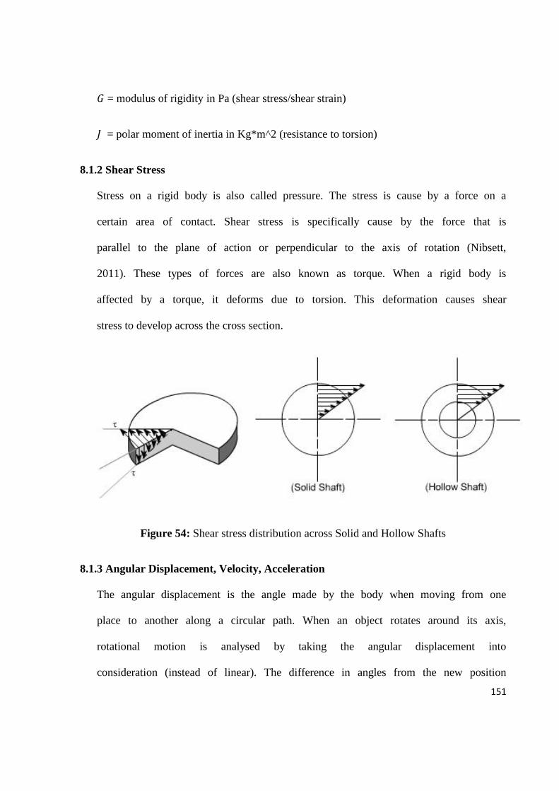
151

𝐺 = modulus of rigidity in Pa (shear stress/shear strain)

𝐽 = polar moment of inertia in Kg*m^2 (resistance to torsion)

8.1.2 Shear Stress

Stress on a rigid body is also called pressure. The stress is cause by a force on a

certain area of contact. Shear stress is specifically cause by the force that is

parallel to the plane of action or perpendicular to the axis of rotation (Nibsett,

2011). These types of forces are also known as torque. When a rigid body is

affected by a torque, it deforms due to torsion. This deformation causes shear

stress to develop across the cross section.

Figure 54: Shear stress distribution across Solid and Hollow Shafts

8.1.3 Angular Displacement, Velocity, Acceleration

The angular displacement is the angle made by the body when moving from one

place to another along a circular path. When an object rotates around its axis,

rotational motion is analysed by taking the angular displacement into

consideration (instead of linear). The difference in angles from the new position

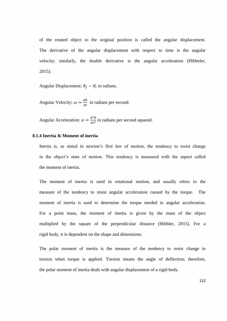
152

of the rotated object to the original position is called the angular displacement.

The derivative of the angular displacement with respect to time is the angular

velocity; similarly, the double derivative is the angular acceleration (Hibbeler,

2015).

Angular Displacement: 𝜃𝑓 − 𝜃𝑖 in radians.

Angular Velocity: 𝜔 =𝑑𝜃

𝑑𝑡 in radians per second.

Angular Acceleration: 𝛼 =𝑑2𝜃

𝑑𝑡2 in radians per second squared.

8.1.4 Inertia & Moment of inertia

Inertia is, as stated in newton’s first law of motion, the tendency to resist change

in the object’s state of motion. This tendency is measured with the aspect called

the moment of inertia.

The moment of inertia is used in rotational motion, and usually refers to the

measure of the tendency to resist angular acceleration caused by the torque. The

moment of inertia is used to determine the torque needed in angular acceleration.

For a point mass, the moment of inertia is given by the mass of the object

multiplied by the square of the perpendicular distance (Hibbler, 2015). For a

rigid body, it is dependent on the shape and dimensions.

The polar moment of inertia is the measure of the tendency to resist change in

torsion when torque is applied. Torsion means the angle of deflection; therefore,

the polar moment of inertia deals with angular displacement of a rigid body.

153

Figure 55: Equations of moment and polar moment of inertia for different shapes of rigid

bodies

8.1.5 Power

Power is the rate of doing work, or the rate of energy/heat transfer. In terms of

rigid bodies, it is the product of the torque multiplied by the angular velocity. It

is measured in Watts or Joules per second.

8.1.6 Density

Density is simply put as the mass of a substance per its unit volume. It is

measured in Kilograms per meters cubed.

8.2 Differential Equations

Solving each type of model require a set number of mathematical skills dealing

with differential equations. In general, there are many ways to solve a differential

equation, but the most used and reliable way in control system engineering is the

frequency response method. The frequency response method utilizes the Laplace

transform to change the differential equation from the time domain to the

154

frequency domain. This change causes the model equations to change from

derivatives to polynomials; and polynomials are much easier to solve from

classic algebra. Now the solved equations can be brought back to the time

domain, but in today’s simulation software, it is possible to study and understand

the behaviour of the model just from the frequency response. Normally there are

two types of differential equations; ordinary and partial. Ordinary equations

would be in terms of one independent and one dependent variable. Partial

differential equations on the other hand, are equations in terms of more than one

independent variable. The Lumped and Finite element drive line mathematical

models utilize ordinary differential equations, while the transmission model

utilises the partial differential equations.

Documents

Simulation & Analysis of the Helicopter Transmission System · Abstract This report analyzes the main shafts of the helicopter transmission box. The corresponding behavior of the