1

Simulating the Simplest Walking Model Using Altair Hyperworks 9.0

Semester Report – Spring 2008 MAE 690 - Master’s of Engineering (M. Eng.) Project

Rohit Hippalgaonkar

rrh54@cornell.edu +1-607-379-3529 +91-40-27565385 3-4-1013/15, Barkatpura Hyderabad, A.P., INDIA - 500027

Masters of Engineering Candidate, August 2008 Sibley School of Mechanical & Aerospace Engineering

Cornell University Ithaca, NY, USA 14853 Biorobotics and Locomotion Lab

Department of Theoretical & Applied Mechanics Cornell University

Ithaca, NY, USA 14853

2

Foreword This report outlines the work I have done over the Spring Semester in the Biorobotics and Locomotion Laboratory at Cornell University while simulating the simplest walking model (Garcia, et al - 1998) using Altair’s Hyperworks 9.0, a dynamic simulation software. The aim of my project was to test the suitability of this software in simulating the kind of walking robots that are built in the lab. Chapter 1 provides an introduction to Hyperworks 9.0, while also outlining the need to pursue the project. Chapter 2 details how the Simplest Walking Model was built in the software, mentioning the specific features used. Chapter 3 sheds light on the results of the simulations and Chapter 4 lists the conclusions that I have drawn based on my experience with the software. I worked about 10 hours per week on the project from February 20, 2008 to June 20, 2008. I started by simulating the simple pendulum, then a double pendulum, and then a bouncing ball (without any horizontal velocity) and performing various successful consistency checks (for e.g. conservation of energy, where applicable) before setting out to build and simulate the simplest walking model. For the simplest walking model itself, I tried two different ways of implementing the collision, using initial conditions that are known to give ‘period-one walking’ (from I).

3

Contents Foreword …………. 2 1. Introduction …………. 4 2. Simulating the Simplest Walker …………. 5 3. Results and Discussion ………….. 13 4. Conclusions …………16 5. References …………. 17 6. Appendices ………… 18

4

1. Introduction The Bio-robotics and locomotion lab specializes in building energy-efficient walking robots and walking toys. Many of these (e.g. the Cornell Ranger, the kneed passive-walking bi-ped, and so on) have been inspired by passive-dynamic walking models (e.g. the Simplest Walking Model (Garcia, et al 1998)). One approach to realizing energy-efficient robots is by finding optimal control laws in simulation that minimize the cost of walking and then implementing these laws on the robot. Simulation of the walking robot is the first step in finding the optimal control laws. This report describes in detail, an attempt at simulating the Simplest Walking Model using Hyperworks, and could serve as a guideline (and hopefully a time-saving tool) to someone building a similar walking model in the future while learning the software from scratch. Typically, the following steps are involved in simulating passive-dynamic walking models: first the governing equations of motion are derived and pieced together with the chosen collision model to form what is called the ‘stride map’. Suppose that a stride is the period starting from the instant of time just before a collision, until the instant just before the next collision. Typically, we are only interested in finding the set of initial conditions (or states) that give the same state before the next collision, i.e. we are only interested in ‘period-one cycles’. These initial conditions are found using root-finding sub-routines. Next, we find the optimal control law by carrying out an energy-minimization optimization, i.e. by finding which control law minimizes the cost of walking. We were looking to find a software or package that has the capability to allow us to perform all these steps, and Altair’s Hyperworks 9.0 seemed a good candidate. Hyperworks 9.0 is an advanced multi-body dynamic simulation software most used in the automobile industry and reportedly has tools or features useful for modeling, analysis, optimization, visualization, reporting and performance data management. For our purposes, one of its most important features is that we don’t have to derive governing equations. In a lot of cases (e.g. in kneed walkers, or walkers based on the triple pendulum) the equations are complex and take a long time to be derived by hand or by using software such as Matlab, Mathematica and so on. Hyperworks takes in a CAD-type model that is built and saved by the user to a .mdl file, using features such as ‘Points’, ‘Bodies’, ‘Markers’, ‘Joints’, ‘Graphics’ and optional features such as ‘Templates’, ‘Contacts’ and ‘Sensors’. The user then sets simulation parameters, such as end time of simulation, integration tolerances, step sizes along with choosing the integrator that will be used, and saves all these along with the model to a .xml file (preferably the same name as the .mdl file), which serves as the solver input file. Running the simulation then creates output files (in .h3d, .plt, .abf and .mrf formats, all with the same first name) that allow you to animate and plot results while a log file (.log) is also created that shows up any errors in the model.

2. Simulating the Simplest Walker In Hyperworks, we use ‘MotionView’, an environment to build multi-body dynamic models. ‘MotionSolve’ is a multi-body solver that is based on the principles of mechanics, and is tightly integrated with MotionView. It takes its input from the .mdl file and .xml files to automatically formulate and solve the equations of motion. The results, or solver output, are then plotted and animated and saved to .abf, .mrf, .h3d and .plt formats. The animation of results is viewed in ‘Hyperview’ and plots in ‘Hypergraph’.

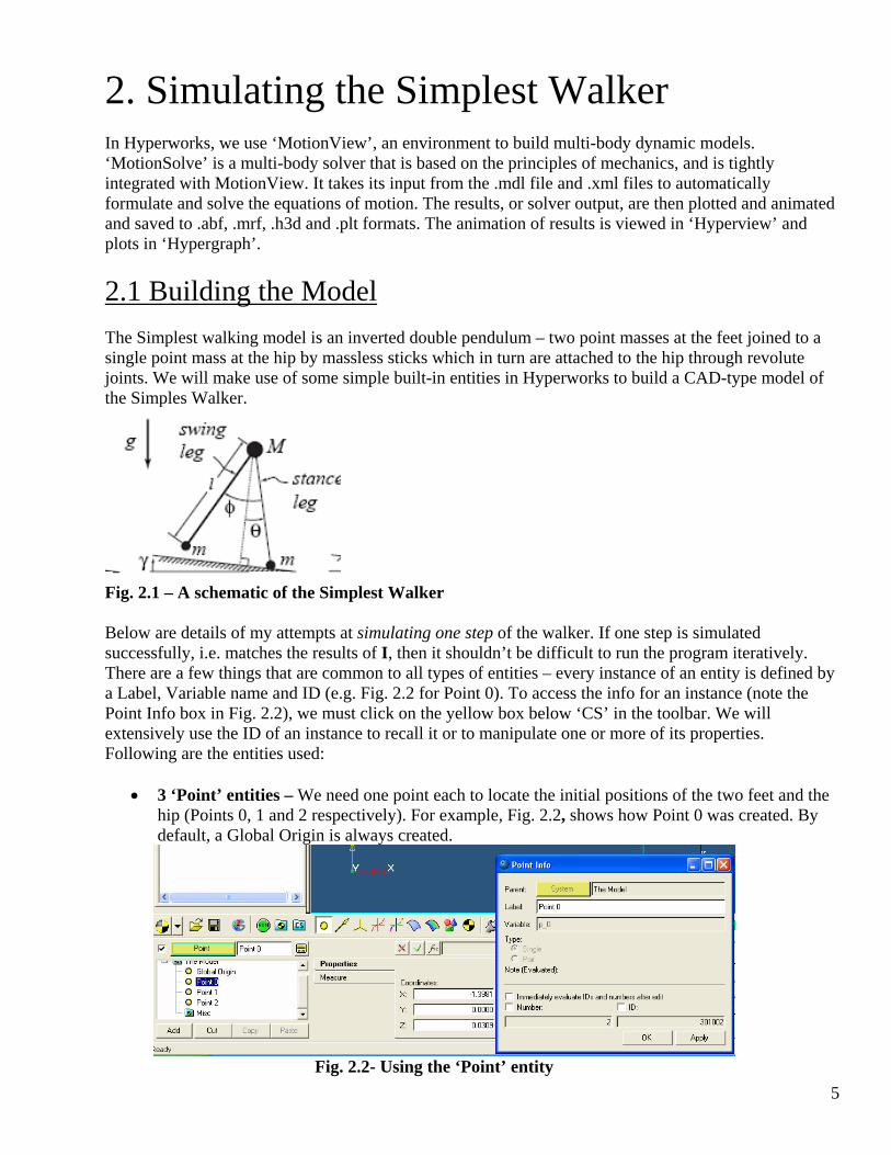
2.1 Building the Model The Simplest walking model is an inverted double pendulum – two point masses at the feet joined to a single point mass at the hip by massless sticks which in turn are attached to the hip through revolute joints. We will make use of some simple built-in entities in Hyperworks to build a CAD-type model of the Simples Walker.

Fig. 2.1 – A schematic of the Simplest Walker Below are details of my attempts at simulating one step of the walker. If one step is simulated successfully, i.e. matches the results of I, then it shouldn’t be difficult to run the program iteratively. There are a few things that are common to all types of entities – every instance of an entity is defined by a Label, Variable name and ID (e.g. Fig. 2.2 for Point 0). To access the info for an instance (note the Point Info box in Fig. 2.2), we must click on the yellow box below ‘CS’ in the toolbar. We will extensively use the ID of an instance to recall it or to manipulate one or more of its properties. Following are the entities used:

• 3 ‘Point’ entities – We need one point each to locate the initial positions of the two feet and the hip (Points 0, 1 and 2 respectively). For example, Fig. 2.2, shows how Point 0 was created. By default, a Global Origin is always created.

Fig. 2.2- Using the ‘Point’ entity

5

• 5 ‘Body’ entities – One body (Body 2, at Point 2) at the hip joining the two legs (‘M’ in Fig 2.1), and two other bodies (Bodies 0 and 1), each made up of a point mass at the foot and a massless rod to make up the leg. One body (Body 3) is required to make up the horizontal floor on which the simplest walker will walk. All Hyperworks models have a default Ground Body (B_Ground). The ‘Body’ entity requires the user to specify which co-ordinate system will be used (in this case, I have used the ‘CM (centre of mass) co-ordinate system’ to be used for all bodies), initial conditions for the body and its basic ‘Properties’, such as its shape, which two points it joins, etc. Note, choose Body 1 to be the stance leg and Body 0 to be the swing leg.

Fig. 2.3- Using the ‘Body’ entity • 5 ‘Marker’ entities – Markers are a set of co-ordinate axes (or frame) that are attached to a

particular body at a specific point. We attach markers to both Body 0 and Body 3 at Point 0, as well as to Bodies 1 and 3 at Point 1. Among the many uses of the markers, one is that they give us the capability of defining ‘floating’ joints (elaborated under ‘Templates’). Again, by default a Global Frame is attached at the Global Origin to the Ground Body.

Fig. 2.4 - Defining a ‘Marker’ entity

• 4 ‘Joint’ entities – We require 1 revolute joint between Body 0 and Body 2 (Joint 02), and one revolute joint between Body 1 and Body 2 (Joint 12). Body 3 is fixed to the ground, so we need a ‘Fixed Joint’ between Body 3 and Ground Body. We also need to start with one leg being the stance leg and the other the swing leg.

Fig. 2.5- Using the ‘Joint’ entity

6

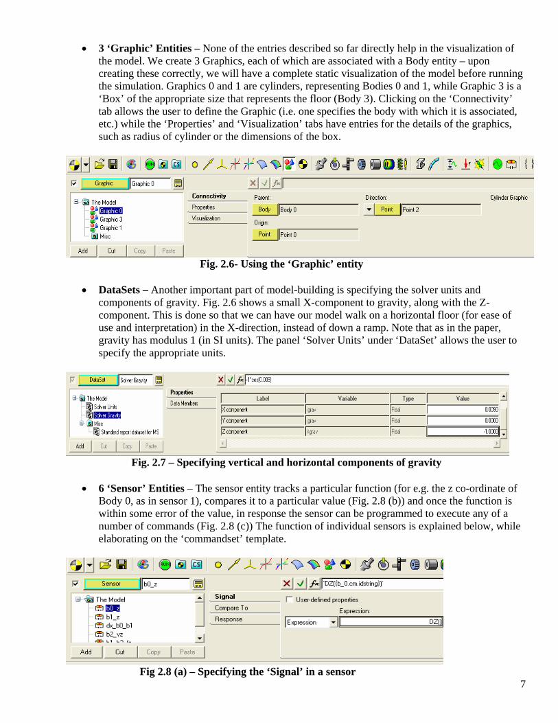
• 3 ‘Graphic’ Entities – None of the entries described so far directly help in the visualization of the model. We create 3 Graphics, each of which are associated with a Body entity – upon creating these correctly, we will have a complete static visualization of the model before running the simulation. Graphics 0 and 1 are cylinders, representing Bodies 0 and 1, while Graphic 3 is a ‘Box’ of the appropriate size that represents the floor (Body 3). Clicking on the ‘Connectivity’ tab allows the user to define the Graphic (i.e. one specifies the body with which it is associated, etc.) while the ‘Properties’ and ‘Visualization’ tabs have entries for the details of the graphics, such as radius of cylinder or the dimensions of the box.

Fig. 2.6- Using the ‘Graphic’ entity

• DataSets – Another important part of model-building is specifying the solver units and components of gravity. Fig. 2.6 shows a small X-component to gravity, along with the Z-component. This is done so that we can have our model walk on a horizontal floor (for ease of use and interpretation) in the X-direction, instead of down a ramp. Note that as in the paper, gravity has modulus 1 (in SI units). The panel ‘Solver Units’ under ‘DataSet’ allows the user to specify the appropriate units.

Fig. 2.7 – Specifying vertical and horizontal components of gravity

• 6 ‘Sensor’ Entities – The sensor entity tracks a particular function (for e.g. the z co-ordinate of Body 0, as in sensor 1), compares it to a particular value (Fig. 2.8 (b)) and once the function is within some error of the value, in response the sensor can be programmed to execute any of a number of commands (Fig. 2.8 (c)) The function of individual sensors is explained below, while elaborating on the ‘commandset’ template.

7 Fig 2.8 (a) – Specifying the ‘Signal’ in a sensor

Figs. 2.8 (b) and (c) –The ‘Compare To’ and ‘Response’ Entries in a Sensor

• ‘Templates’ – Templates are user-defined blocks of code, written in Templex – a general

purpose text and numeric processor, that comes with Hyperworks. I used them mostly for mathematical programming and declaring variables. Now that we have all the entities we need to build the model, using the set of initial conditions from I (that is known to give period-one walking), we should be able to run a simulation of the simplest walking model. However we still need some high-level control of the simulation. For example, the simplest walker scuffs for a finite amount of time around the instant when the stance leg is vertical, with the chosen initial conditions. Our simulations must ignore this scuffing. The ‘commandset’ template is the tool we will use for this high-level control, and its text is written to the solver command file. Sections 1 and 2 of the ‘commandset’ template (in Appendix 1) are roughly the same in both methods of implementing the collision. To start with, section 1 deactivates all sensors, joints and contacts except Sensor with ID 301004 (which returns to the solver command file once the z-component of the hip’s velocity goes below zero) and Joint 301004 (connecting Body 1 and Body 3). End time is set to 15 seconds, which is much longer than the walking cycle we expect to get (about 3.8 seconds). Once Sensor 301004 returns to the solver command file, it is deactivated in section 2. We then check that it is indeed Body1 that is the stance leg with an ‘if’ condition and then activate Sensor 301003 that returns to the command file once Point 0 is ahead of Point 1 by a certain amount (0.25 mts). This ensures that scuffing is ignored and that collision is implemented only after the swing leg is ahead of the stance leg by a good amount. The remaining sections of the template differ depending on the way we want to implement the collision (however Sensor 301003 must be deactivated first in both methods).

2.2 Implementing Collision Below are outlined two different ways that I attempted to implement collision at the end of step:

1) Using Contacts – The collision of the walker with the floor can be implemented by using the built-in ‘Contact’ entity (Fig. 2.9), which implements a collision through a spring-damper type system. We will need a ‘contact’ at each foot with the floor, and Hyperworks requires it to be defined between a pair of graphics (not bodies). The co-efficient of restitution controls the damping and needs to be close to zero in the case of the simplest walker. The penalty is like the spring constant – if it is too high, then the body jumps up too high after collision and if it is too low then the body penetrates too deep through the floor. Coulomb friction can be turned off or on, along with the related parameters – static and dynamic coefficients of friction, and the stiction and friction transition velocities.

8

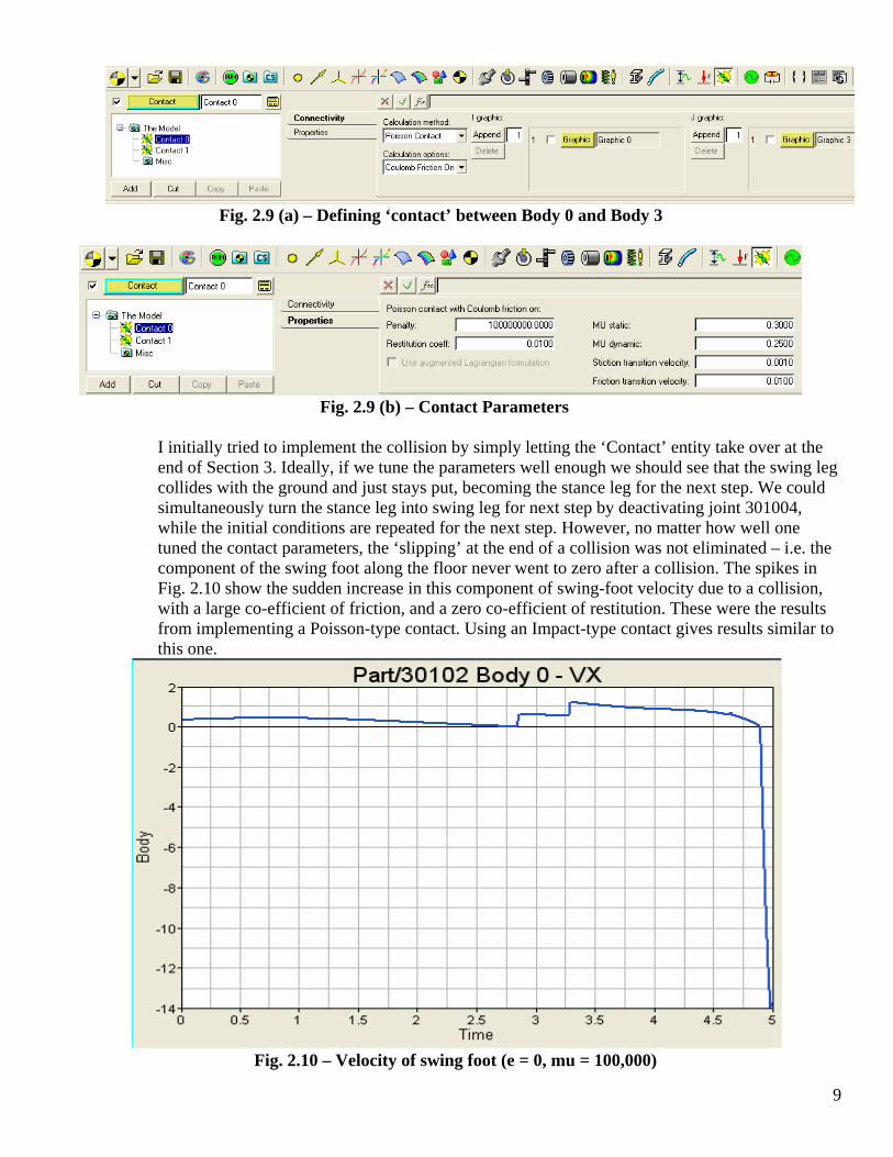
Fig. 2.9 (a) – Defining ‘contact’ between Body 0 and Body 3

Fig. 2.9 (b) – Contact Parameters

I initially tried to implement the collision by simply letting the ‘Contact’ entity take over at the end of Section 3. Ideally, if we tune the parameters well enough we should see that the swing leg collides with the ground and just stays put, becoming the stance leg for the next step. We could simultaneously turn the stance leg into swing leg for next step by deactivating joint 301004, while the initial conditions are repeated for the next step. However, no matter how well one tuned the contact parameters, the ‘slipping’ at the end of a collision was not eliminated – i.e. the component of the swing foot along the floor never went to zero after a collision. The spikes in Fig. 2.10 show the sudden increase in this component of swing-foot velocity due to a collision, with a large co-efficient of friction, and a zero co-efficient of restitution. These were the results from implementing a Poisson-type contact. Using an Impact-type contact gives results similar to this one.

Fig. 2.10 – Velocity of swing foot (e = 0, mu = 100,000)

9

I then tried another approach (Section 3 onwards in Appendix 1) wherein one follows a similar approach as above, except that a joint was activated at the swing foot at the instant when it is rebounding upwards and at the height of the floor. For this we activate Sensor 301006, which returns to the command file once the velocity of the swing foot goes above zero. Since we turn on this sensor only after turning off sensor 301003 (i.e. swing foot is ahead of stance foot by a good amount), the swing foot is already on its way down. The only way it can have an upward component of velocity is after the collision. In Section 4, once Sensor 301006 returns, we activate a sensor (301005) that returns when the swing foot is above the floor. Next in section 5, we simultaneously activate joint (301005) at swing foot and deactivate joint (301004) at the stance foot while also deactivating sensor 301005. Simulation is then re-started.

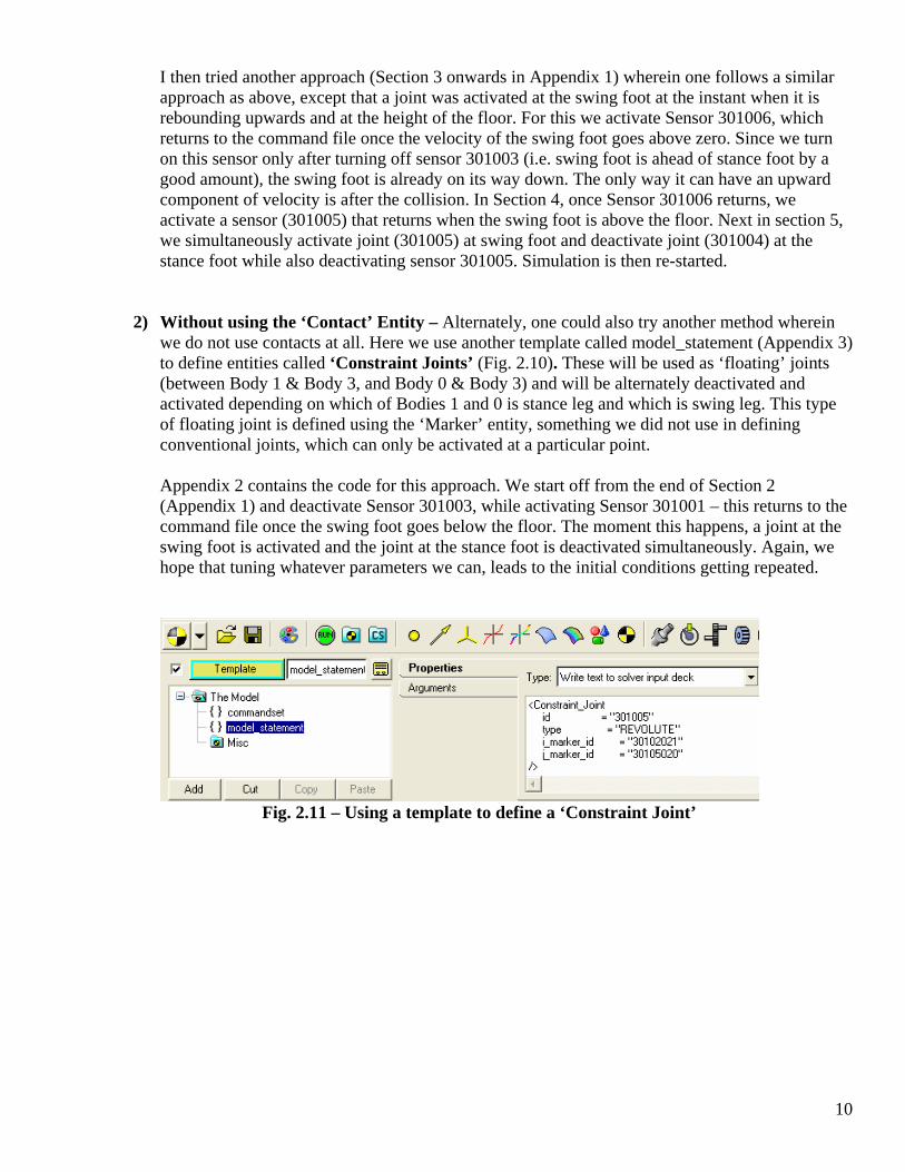
2) Without using the ‘Contact’ Entity – Alternately, one could also try another method wherein we do not use contacts at all. Here we use another template called model_statement (Appendix 3) to define entities called ‘Constraint Joints’ (Fig. 2.10). These will be used as ‘floating’ joints (between Body 1 & Body 3, and Body 0 & Body 3) and will be alternately deactivated and activated depending on which of Bodies 1 and 0 is stance leg and which is swing leg. This type of floating joint is defined using the ‘Marker’ entity, something we did not use in defining conventional joints, which can only be activated at a particular point.

Appendix 2 contains the code for this approach. We start off from the end of Section 2 (Appendix 1) and deactivate Sensor 301003, while activating Sensor 301001 – this returns to the command file once the swing foot goes below the floor. The moment this happens, a joint at the swing foot is activated and the joint at the stance foot is deactivated simultaneously. Again, we hope that tuning whatever parameters we can, leads to the initial conditions getting repeated.

Fig. 2.11 – Using a template to define a ‘Constraint Joint’

10

2.3 Running the Simulation Once model-building is complete, we save the .xml file with the same first name as the .mdl file, by clicking on the ‘Main’ tab under the ‘Run’ button in the toolbar (Fig. 2.12 (a)). Next the ‘Simulation Parameters’ are set (Fig. 2.12 (b)) and a ‘Transient’ type simulation is chosen with the appropriate parameters (Fig. 2.12 (c)) – minimum and maximum step-sizes, integration tolerances, etc.

Fig. 2.12 (a) – Saving the XML file

Fig. 2.12 (b) – Simulation Parameters

Fig. 2.12 (c) – ‘Transient’ type Simulation Next, click on ‘Check’ (in the far right corners of Fig. 2.11) – this opens up the Message Log, which shows up the results of checking the model. This points to any obvious modeling errors such as syntax errors and so on. Clicking on the ‘Run’ button under the ‘Check’ button (above) actually puts MotionSolve into action, where the equations are automatically derived from the .mdl and .xml files and solved. A commentary on the results of the simulation(s) is displayed in a windows prompt – this is a helpful feature in detecting the more subtle errors in modeling (which do not show up at the end of the model ‘Check)’, or arriving at the reasons behind the inability of the solver to accurately solve the system (Fig. 2.13 shows a section of the output). These comments are also saved in the .log file with the same first name as the .mdl file, which is automatically created when the ‘Run’ button (above) is clicked.

11

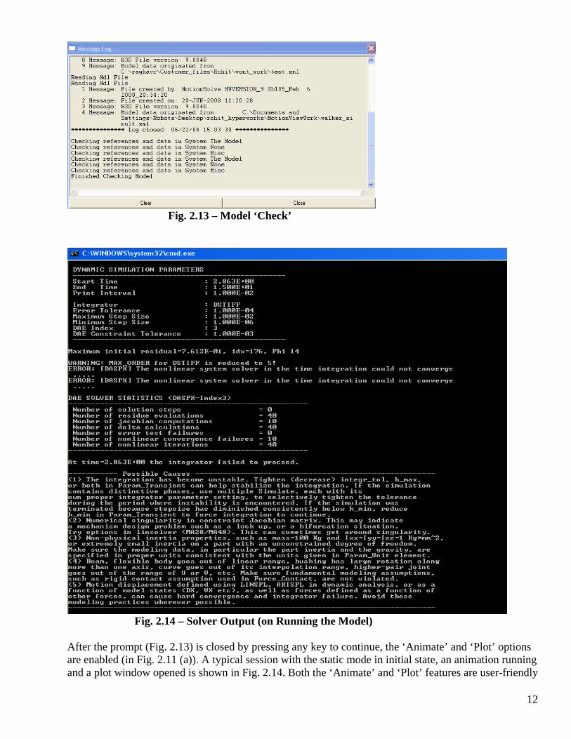
Fig. 2.13 – Model ‘Check’

Fig. 2.14 – Solver Output (on Running the Model) After the prompt (Fig. 2.13) is closed by pressing any key to continue, the ‘Animate’ and ‘Plot’ options are enabled (in Fig. 2.11 (a)). A typical session with the static mode in initial state, an animation running and a plot window opened is shown in Fig. 2.14. Both the ‘Animate’ and ‘Plot’ features are user-friendly

12

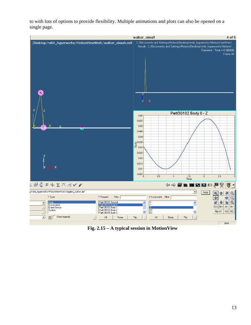
to with lots of options to provide flexibility. Multiple animations and plots can also be opened on a single page.

Fig. 2.15 – A typical session in MotionView

13

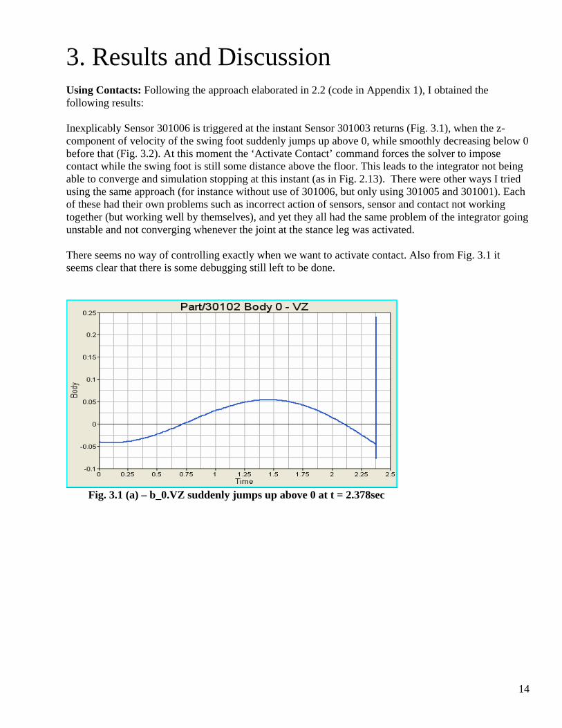
3. Results and Discussion Using Contacts: Following the approach elaborated in 2.2 (code in Appendix 1), I obtained the following results: Inexplicably Sensor 301006 is triggered at the instant Sensor 301003 returns (Fig. 3.1), when the z-component of velocity of the swing foot suddenly jumps up above 0, while smoothly decreasing below 0 before that (Fig. 3.2). At this moment the ‘Activate Contact’ command forces the solver to impose contact while the swing foot is still some distance above the floor. This leads to the integrator not being able to converge and simulation stopping at this instant (as in Fig. 2.13). There were other ways I tried using the same approach (for instance without use of 301006, but only using 301005 and 301001). Each of these had their own problems such as incorrect action of sensors, sensor and contact not working together (but working well by themselves), and yet they all had the same problem of the integrator going unstable and not converging whenever the joint at the stance leg was activated. There seems no way of controlling exactly when we want to activate contact. Also from Fig. 3.1 it seems clear that there is some debugging still left to be done.

Fig. 3.1 (a) – b_0.VZ suddenly jumps up above 0 at t = 2.378sec

14

Fig. 3.1 (b) – Sensor 301006 triggered (at t = 2.378 sec) Without Using Contacts: Fig. 2.13 shows the error messages that showed up with this kind of approach and Fig. 2.14 shows the output. The solver could not converge once the joint was imposed (at t = 2.863 sec, as soon as Sensor 301001 returns to the command file). The integrator stops at this point and cannot go any further. This time though, the stance foot is at the floor level (as indicated by the return of Sensor 301001), unlike when we were imposing collision with contacts. One reason why this is happening could be because of bugs in the program, or alternately it could be because the joint is not appropriately defined. The joint in question, 301005, is a revolute joint between swing leg and floor, which was defined through markers (in model_statement). These markers were attached to both bodies at Point 0 (swing foot) in the initial state. While Point 0 on the swing foot is moving, it is static on Body 3 (which is the floor). This could be the reason for the non-convergence of the solver as the two markers are too far apart for the joint to impose a constraint. However, this was the only way I could imagine it could work and I have not found a way of defining joints on-the-fly. Another possibility would be to place joints on the floor beforehand at points where we know the swing foot would collide and activate joints between these points and the swing foot. Ofcourse, this would be cumbersome if one would want to test the walker for many steps.

15

16

4. Conclusions Overall, the software does not seem completely bug-free yet. Even if it were, it does not give the user the capability to implement ‘joints’ and ‘contacts’ at will. Syntax errors were easy enough to detect but hard to fix. In some cases, a small error such as having an extra space in between two commas shows up an error without explicitly saying what the error was. On the positive side, Hyperworks is a great interface for analysis with its advanced animation and plotting capabilities. The plotting features can be used effectively for error-diagnosis. The .log file created also gives good feedback in terms of warnings and errors, and helps reduce the amount of time you might spend on debugging. In terms of its use to model walking robots, it can do a good job once collisions can be implemented accurately. Once we know what initial conditions to start with, it can easily simulate robots with lots of parts (such as the Cornell Ranger). I could not get to root-finding being stuck with implementation of collision for the most part, so it would be hard to draw conclusions on its capability to do the same. However, it does have the option of creating script files (just like .m files in Matlab), in TCL / TK. In terms of implementing control, Hyperworks only has SISO-control capability. So, for example, ‘Jacobian-killer’ control cannot be implemented in the current version.

17

References and Resources I. Garcia, M., Chatterjee, A., Ruina, A., and Coleman, M. (1997), ‘The Simplest Walking Model: Stability, Complexity, and Scaling’, ASME Journal of Biomechanical Engineering. II. Altair Engineering, ‘MotionView Training Volumes I & II , and MotionSolve Introduction’, Altair Hyperworks 8.0 Training Manual. III. Zapgrab2 Software

18

Appendix 1 The full code for the ‘commandset’ template while implementing collisions using ‘Contacts’: % Section 1 <H3DOutput switch_on = "TRUE" increment = "1" start_time = "0." end_time = "9999999." format_option = "AUTO" stress_option = "TENSOR" strain_option = "TENSOR" /> <Param_Simulation constr_tol = "1.0000E-10" implicit_diff_tol = "1.0000E-06" /> <Param_Transient integr_tol = "0.0001" integrator_type = "DSTIFF" h_max = "0.01" h0_max = "0.001" /> <Deactivate element_type = "SENSOR" element_id = "301001" /> <Deactivate element_type = "SENSOR" element_id = "301002" /> <Deactivate element_type = "SENSOR" element_id = "301003" /> <Deactivate element_type = "SENSOR" element_id = "301005" /> <Deactivate element_type = "CONTACT" element_id = "301001" /> <Deactivate element_type = "CONTACT" element_id = "301002" /> <Deactivate element_type = "JOINT" element_id = "301005" /> <Deactivate element_type = "JOINT" element_id = "301006" /> <Simulate analysis_type = "Transient"

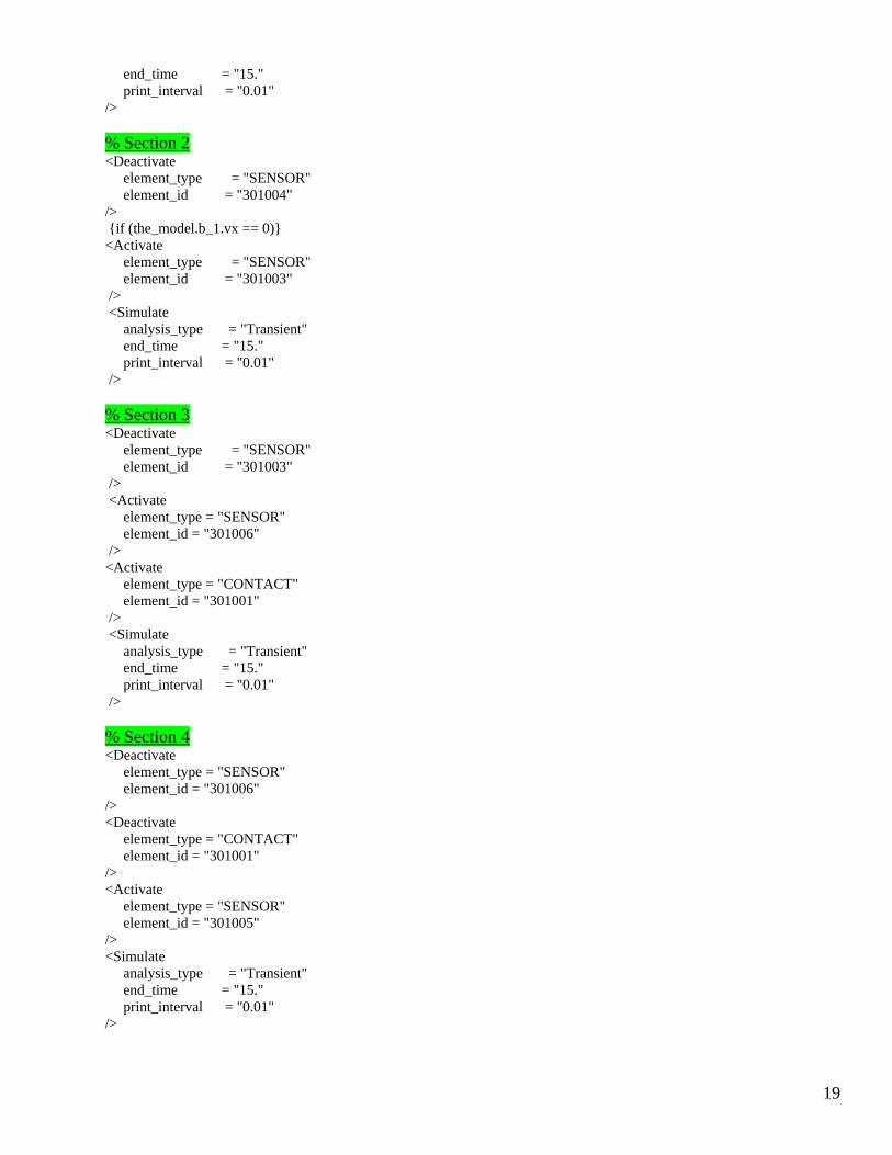
19

end_time = "15." print_interval = "0.01" /> % Section 2 <Deactivate element_type = "SENSOR" element_id = "301004" /> {if (the_model.b_1.vx == 0)} <Activate element_type = "SENSOR" element_id = "301003" /> <Simulate analysis_type = "Transient" end_time = "15." print_interval = "0.01" /> % Section 3 <Deactivate element_type = "SENSOR" element_id = "301003" /> <Activate element_type = "SENSOR" element_id = "301006" /> <Activate element_type = "CONTACT" element_id = "301001" /> <Simulate analysis_type = "Transient" end_time = "15." print_interval = "0.01" /> % Section 4 <Deactivate element_type = "SENSOR" element_id = "301006" /> <Deactivate element_type = "CONTACT" element_id = "301001" /> <Activate element_type = "SENSOR" element_id = "301005" /> <Simulate analysis_type = "Transient" end_time = "15." print_interval = "0.01" />

20

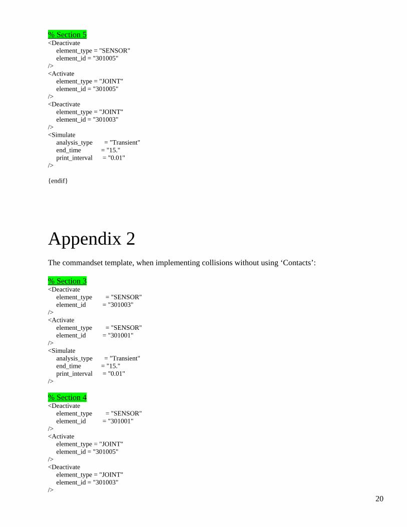
% Section 5 <Deactivate element_type = "SENSOR" element_id = "301005" /> <Activate element_type = "JOINT" element_id = "301005" /> <Deactivate element_type = "JOINT" element_id = "301003" /> <Simulate analysis_type = "Transient" end_time = "15." print_interval = "0.01" /> {endif}

Appendix 2 The commandset template, when implementing collisions without using ‘Contacts’: % Section 3 <Deactivate element_type = "SENSOR" element_id = "301003" /> <Activate element_type = "SENSOR" element_id = "301001" /> <Simulate analysis_type = "Transient" end_time = "15." print_interval = "0.01" /> % Section 4 <Deactivate element_type = "SENSOR" element_id = "301001" /> <Activate element_type = "JOINT" element_id = "301005" /> <Deactivate element_type = "JOINT" element_id = "301003" />

21

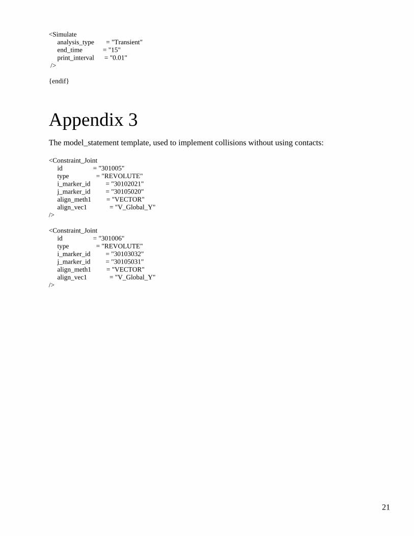
<Simulate analysis_type = "Transient" end_time = "15" print_interval = "0.01" /> {endif}

Appendix 3 The model_statement template, used to implement collisions without using contacts: <Constraint_Joint id = "301005" type = "REVOLUTE" i_marker_id = "30102021" j_marker_id = "30105020" align_meth1 = "VECTOR" align_vec1 = "V_Global_Y" /> <Constraint_Joint id = "301006" type = "REVOLUTE" i_marker_id = "30103032" j_marker_id = "30105031" align_meth1 = "VECTOR" align_vec1 = "V_Global_Y" />