Embed Size (px)
Citation preview

SimulatingHearing LossUsing aTransmission LineCochleaModelL. Koop
;


SimulatingHearing Loss
Using aTransmission Line Cochlea Model
by
L. Koopto obtain the degree of Master of Applied Mathematics
in the faculty of EEMCS at the Delft University of Technology,to be defended publicly on Thursday October 29, 2015 at 11:00 AM.
Student number: 4424387Project duration: September 24, 2014 – October 29, 2015Thesis committee: Prof. dr. ir. C. Vuik, TU Delft, supervisor
Dr. ir. P. W. J. van Hengel, INCAS3, supervisorDr. J. L. A. Dubbeldam, TU Delft
An electronic version of this thesis is available at http://repository.tudelft.nl/.


Preface
On the afternoon of June 26, 2001 I lived through a traumatic experience which profoundly impacted thedirection my life would take. In the thirty minutes, during which time the life of my sister seemed to hangin the balance and the memory of which is distorted by adrenaline, my life went from quiet, to exceedinglychaotic, and then back to a promise of normality. That day taught me the value of life and I also saw quality oflife in a new light. The events of that day impacted my decision to go through a rigorous Emergency MedicalTechnician (EMT) training, volunteer time to Emergency Medical Services, and when given the opportunity,to conduct research in medically related fields.
While enrolled at the Full-time Training in Anaheim, a graduate level bible college, I worked on theiraudio visual team. Therefore, armed with medical training and an interest in audio engineering the topic of“Simulating Hearing Loss” piqued my interest.
This topic of research was proposed by the research institute INCAS3 based in Assen. It is therefore:
An INCAS3 project.
The human ear is a very complex organ and there are many phenomena like the cochlear amplifier andvarious otoaucustic emissions that we are just beginning to understand. It is only logical to use models ofthe inner ear to simulate hearing loss in order to incorporate as many of the interdependent phenomena aspossible. In this ground breaking research a transmission line cochlea model was used to simulate a damagedcochlea and a backward transformation method was developed to allow for sound to be reconstructed fromthe model of a damaged cochlea. Even early results show that this method for simulating hearing loss allowsfor the affects of a damaged region to be propagated to an area in the cochlea that is not damaged. This is asignificant advantage over pure signal processing based hearing loss simulation.
Because this type of simulation had not been successful previously, some unforeseen complications alsoarose with the mathematical model that was believed to be tried and tested. For the back transformation ofthe sound to be possible, an energy handling flaw in the model first needed to be corrected.
My work on this project would not have succeeded if not for the help from many people. Most importantlyI would like to thank Peter van Hengel for answering countless questions, pointing out helpful study mate-rial, and providing valuable feedback. Kees Vuik also helped in many ways, was always available to answerquestions, and most importantly asked good questions in return.
Henk and Tamara, if it were not for your home, Delft would have been a lonelier place. To Pieter and LilianRodenburg, being able to come and help with the farm work was a great and needed study break. Jacob andPriscilla, as well as Roger, thank you for visiting me all the way from Belize. I shall always remember our timetogether in Europe fondly. To the Nieuwelink families in Vlaardingen, thank you for all the times that you hadme in your homes. Without all of you this project would not have been successful.
L. KoopDelft, October 2015
iii


Contents
0.1 Acronyms . . . . . . . . . . . . . . . . . . . . . . . . . . . . . . . . . . . . . . . . . . . . . 10.2 Definitions . . . . . . . . . . . . . . . . . . . . . . . . . . . . . . . . . . . . . . . . . . . . 1
1 Introduction 31.1 Research Question . . . . . . . . . . . . . . . . . . . . . . . . . . . . . . . . . . . . . . . . 31.2 Report Map . . . . . . . . . . . . . . . . . . . . . . . . . . . . . . . . . . . . . . . . . . . . 4
2 Hearing andHearing Loss 52.1 Components of the Hearing System. . . . . . . . . . . . . . . . . . . . . . . . . . . . . . . . 5
2.1.1 The Outer and Middle Ear . . . . . . . . . . . . . . . . . . . . . . . . . . . . . . . . . 52.1.2 The Cochlea . . . . . . . . . . . . . . . . . . . . . . . . . . . . . . . . . . . . . . . . 52.1.3 The Frequency Map . . . . . . . . . . . . . . . . . . . . . . . . . . . . . . . . . . . . 62.1.4 The Cochlear Nerve . . . . . . . . . . . . . . . . . . . . . . . . . . . . . . . . . . . . 7
2.2 Cochlear Emissions . . . . . . . . . . . . . . . . . . . . . . . . . . . . . . . . . . . . . . . . 72.2.1 Distortion Product Otoacoustic Emissions (DPOAEs) . . . . . . . . . . . . . . . . . . . 82.2.2 Spontanious Otoacoustic Emissions (SOAEs) . . . . . . . . . . . . . . . . . . . . . . . 82.2.3 Cochlear Amplifier . . . . . . . . . . . . . . . . . . . . . . . . . . . . . . . . . . . . . 8
2.3 Hearing Loss . . . . . . . . . . . . . . . . . . . . . . . . . . . . . . . . . . . . . . . . . . . 82.3.1 Age. . . . . . . . . . . . . . . . . . . . . . . . . . . . . . . . . . . . . . . . . . . . . 82.3.2 Noise Exposure . . . . . . . . . . . . . . . . . . . . . . . . . . . . . . . . . . . . . . 92.3.3 Inner Hair Loss. . . . . . . . . . . . . . . . . . . . . . . . . . . . . . . . . . . . . . . 92.3.4 Outer Hair Loss . . . . . . . . . . . . . . . . . . . . . . . . . . . . . . . . . . . . . . 92.3.5 Auditory Deafferentation . . . . . . . . . . . . . . . . . . . . . . . . . . . . . . . . . 92.3.6 Other Hearing Problems . . . . . . . . . . . . . . . . . . . . . . . . . . . . . . . . . . 9
3 Modeling the Cochlea 113.1 Coupled Oscillators as the Spatial Discretization . . . . . . . . . . . . . . . . . . . . . . . . . 123.2 A Linear Model . . . . . . . . . . . . . . . . . . . . . . . . . . . . . . . . . . . . . . . . . . 12
3.2.1 A Linear Parameter Set . . . . . . . . . . . . . . . . . . . . . . . . . . . . . . . . . . . 143.2.2 Shortcomings of a Linear Model . . . . . . . . . . . . . . . . . . . . . . . . . . . . . . 14
3.3 A Nonlinear Model . . . . . . . . . . . . . . . . . . . . . . . . . . . . . . . . . . . . . . . . 153.3.1 The Parameter Set used by Epp et al. . . . . . . . . . . . . . . . . . . . . . . . . . . . . 15
3.4 Model Inputs and Outputs . . . . . . . . . . . . . . . . . . . . . . . . . . . . . . . . . . . . 17
4 SolutionMethod 214.1 Convolution and Deconvolution vs. Multiplication and Division . . . . . . . . . . . . . . . . . 214.2 The Cochlea Model as a Convolution . . . . . . . . . . . . . . . . . . . . . . . . . . . . . . . 21
4.3 Previous Work by incas3 . . . . . . . . . . . . . . . . . . . . . . . . . . . . . . . . . . . . . 224.4 Sound Resynthesis in the Frequency Domain . . . . . . . . . . . . . . . . . . . . . . . . . . . 224.5 Sound Resynthesis in the Time Domain. . . . . . . . . . . . . . . . . . . . . . . . . . . . . . 23
5 Requirements for Simulating Hearing Loss 255.1 The Choice of Window and Length of Impulse Response . . . . . . . . . . . . . . . . . . . . . 25
5.1.1 Optimal Length of Impulse Response . . . . . . . . . . . . . . . . . . . . . . . . . . . 265.2 Scaling of the Model and N . . . . . . . . . . . . . . . . . . . . . . . . . . . . . . . . . . . . 285.3 Using a Repeated Signal. . . . . . . . . . . . . . . . . . . . . . . . . . . . . . . . . . . . . . 29
5.3.1 Using a Repeated Signal . . . . . . . . . . . . . . . . . . . . . . . . . . . . . . . . . . 295.3.2 Actual Effects of a Repeated Signal . . . . . . . . . . . . . . . . . . . . . . . . . . . . . 30
5.4 Energy Reflection . . . . . . . . . . . . . . . . . . . . . . . . . . . . . . . . . . . . . . . . . 305.4.1 The Problem . . . . . . . . . . . . . . . . . . . . . . . . . . . . . . . . . . . . . . . . 305.4.2 The Solution . . . . . . . . . . . . . . . . . . . . . . . . . . . . . . . . . . . . . . . . 335.4.3 The Best Solution . . . . . . . . . . . . . . . . . . . . . . . . . . . . . . . . . . . . . 37
v

vi Contents
6 Results and Simulations 416.1 Effects of Choice of Oscillator . . . . . . . . . . . . . . . . . . . . . . . . . . . . . . . . . . . 416.2 Combining the Resynthesized Sound . . . . . . . . . . . . . . . . . . . . . . . . . . . . . . . 466.3 Filtering for Combining the Result . . . . . . . . . . . . . . . . . . . . . . . . . . . . . . . . 486.4 Filtering in the Frequency Domain . . . . . . . . . . . . . . . . . . . . . . . . . . . . . . . . 506.5 Scaling the Result . . . . . . . . . . . . . . . . . . . . . . . . . . . . . . . . . . . . . . . . . 506.6 Simulating Hearing Loss . . . . . . . . . . . . . . . . . . . . . . . . . . . . . . . . . . . . . 516.7 The Damaged Sound . . . . . . . . . . . . . . . . . . . . . . . . . . . . . . . . . . . . . . . 566.8 The Low Frequencies . . . . . . . . . . . . . . . . . . . . . . . . . . . . . . . . . . . . . . . 586.9 Number of Representing Oscillators . . . . . . . . . . . . . . . . . . . . . . . . . . . . . . . 58
7 Conclusion 617.1 Discussion . . . . . . . . . . . . . . . . . . . . . . . . . . . . . . . . . . . . . . . . . . . . 617.2 Recommendations . . . . . . . . . . . . . . . . . . . . . . . . . . . . . . . . . . . . . . . . 617.3 The End . . . . . . . . . . . . . . . . . . . . . . . . . . . . . . . . . . . . . . . . . . . . . . 62
A MatLab Code for Sound Resynthesis 63B MatLab Code for the Updated CochleaModel 69Bibliography 81

List of Acronyms and Definitions
0.1. AcronymsCM Cochlear model or model of the cochleaCP Cochlear PartitionCT Combination ToneDCP Digital signal processingDPOAE Distortion Product Otoacoustic EmissionFFT Fast Fourier transformFIR Or FIR filter corresponds to Finite impulse response filterFT Fourier transformIFFT Inverse fast Fourier transformIFT Inverse Fourier transformODE Ordinary Differential EquationRK4 4 step Runge-Kutta methodSOAE Spontaneous Otoacoustic Emission
0.2. DefinitionsCochlea The cochlea is in the inner ear and is the organ that transduces sound coming into the ear
into nerve signalsCochlearpartition
The term used when the Basilar membrane, Reissner’s membrane, and the scala media of thecochlea are all together viewed simply as the partition between the scala vestibuli and scalatympani
1


1Introduction
Hearing loss is a significant disability and can greatly decrease the quality of life. In February of this yearthe World Health Organization published a news release with this stark title “1.1 Billion People at Risk ofHearing Loss”[11]. The main reason for this is the use of personal audio devices. Of course hearing loss isnot something new, but due to the recent increase in noise exposure because of the increased use of music inpopular culture, the relevance of caring for the hearing disabled will be catapulted to new importance. Thisin turn increases the importance of proper modeling of hearing and hearing damage. Accurate simulationof hearing loss could be used to aid in prevention and education, as well as faster development of improvedhearing aids. Fortunately, with the advent of the computer, attempts have been made to simulate hearingloss, but most fall short of truly simulating what a hearing disabled person hears.
The human ear is a remarkable and also an exceedingly complex organ. Trying to simulate hearing lossis certainly not a new endeavor. However, the current typical simulator focuses mainly on a digital signalprocessing approach without the mechanics of the ear being taken into account. In such an approach thesound signal will be edited for certain frequency ranges. This helps to give an impression of what hearing lossmay sound like. But such an approach will not be able to really capture the interdependent nature of damagein the hearing system.
To really be able to capture hearing loss with realism, a new approach to simulating hearing loss is neces-sary, an approach that simulates the physical mechanics of the ear as closely as possible. Of the three partsof the ear (to be introduced in Chapter 2) this report will focus largely on the inner ear, also known as thecochlea. A transmission line type mathematical model of the cochlea is central to the method of simulat-ing hearing loss in the approach taken here. Because sound has not before been successfully resynthesizedfrom this type of model, the new techniques developed will facilitate an entirely new approach to simulatinghearing loss.
1.1. Research QuestionThe goal of the research project “Simulating Hearing Loss” is to resynthesize sound from a transmission linecochlea model of a damaged cochlea. Specific attention will be given to the minimization of sound artifacts.
In the case of the linear model there are a number of things that will need to be considered. One approachto getting the sound from the model is to use a so called inverse filter method (see Section 4.3). For thismethod the CM is viewed as a sound filter. Then in a very similar way as described in Section 4.1 an inversefilter can be found and the original sound is reconstructed. With this method some things that need to beconsidered are the effects that the following have on the quality of sound reconstruction
• Choice of oscillator(s)
• Choice of window
• Breadth of window
• Length of impulse response
• Number of oscillators in the CM
3

4 1. Introduction
• How to combine the results from the different oscillators effectively
• The best way to reduce sound artifacts
• If there is an effect of using a repeated signal
1.2. Report MapThis report is divided into sections as follows. In Chapter 2 the reader is guided through the anatomy of thehuman ear. It explains the functions of the different components of the auditory system. Common physio-logical damages that lead to hearing loss are also presented. Because the models of the cochlea play such acentral role in hearing loss simulation, Chapter 3 examines both linear and nonlinear models of the cochlea.(An original goal of this project was to also include nonlinear cochlea models.) Chapter 4 gives a broad pictureof the solution method as well as the algorithms used. Both frequency domain variants and also time domainvariants of the algorithms are considered. The differences between the two is also explained. Chapter 5 thenexamines the changes that were made to the cochlea model in order for sound reconstruction to work. InChapter 6 the results of the sound reconstructions and hearing loss simulations are presented. The benefitsof using this simulation technique is also pointed out. A final discussion, recommendations for future work,and conclusions are found in Chapter 7. Finally, for the reader interested in the MatLab source code, it isprovided in appendices A and B.

2Hearing and Hearing Loss
Of the five senses hearing is perhaps the one that contributes the most to one’s situational awareness as wellas our complex social interaction skills. It is therefore no surprise that any deterioration of hearing directlyimpacts the quality of life.
2.1. Components of the Hearing SystemThe main components of the auditory system are the outer ear, the middle ear, and the inner ear. The outerear functions to funnel sound into the ear and is composed of the pinna and the ear canal. The middleear transfers sound vibrations from the eardrum to the oval window of the inner ear or cochlea. Within thecochlea sound is neurally encoded to be transmitted to the brain via the cochlear nerve. See Figure 2.1.
2.1.1. The Outer and Middle EarThe outer ear, consisting of the pinna, which we see, and the ear canal directs sound into our ear. The outerear ends at the ear drum. Internal to the eardrum is the middle ear. Within the hollow cavity of the middle earare three bones the malleus, the incus, and the stapes which are also known as the hammer, the anvil and thestirrup respectively. Together these bones are known as the ossicles. Of these bones the malleus is connectedto the eardrum and the stapes is connected to, or rests on, the oval window of the inner ear. These bonesallow for accurate sound wave transfer from the air-filled outer ear to the fluid-filled inner ear. If it were notfor this mechanism then much of the sound would bounce away from the ear without making the air to fluidtransition. The one remaining thing that we should point out here is that there are two muscles connected tothese bones, the stapedius muscle and the tympani muscle. These muscles allow loud sound transfer to theinner ear to be damped when they contract in response to loud sounds.
2.1.2. The CochleaThe inner ear consists of the vestibular system and the cochlea. The vestibular system enhances our balanc-ing ability and is not related to hearing. Because of this, little attention will be given to it. The cochlea onthe other hand will take center stage for much of this report. The cochlea is a coiled tube that resembles theshape of a snail. Within the cochlea are three chambers. The superior (superior versus inferior is medicalterminology for a part of the body that is above or below another part of the body when the body is in a natu-ral standing position) chamber is the scala vestibule and the inferior chamber is the scala tympani. Betweenthese two is the scala media in which is the organ of Corti which contains the hair cells that sense the soundvibrations coming into the cochlea. The hair cells in the organ of Corti then transduce these pressure wavesto action potentials. The action potentials travel to the brain as electrical stimulus via the cochlear nerve. Thescala vestibuli and the scala tympani are connected at the apex. All three chambers of the cochlea are fluidfilled. Both the scala vestibuli and the scala tympani are filled with perilymph and the scala media is filledwith endolymph. These fluids are mechanically equivalent to water. They differ however in chemical com-position, which is key to creating a potential difference over the hair cells, which is essential in the creation ofnerve signals from the motion of the organ of Corti.
The two ends of the cochlea are referred to as the base, near the middle ear, and the apex, at the tip of thespiral. At the base are two membranes, the oval window (or fenestra ovalis) and the round window. The stapes
5

6 2. Hearing and Hearing Loss
Figure 2.1: The human ear. Image source: [13]
bone from the middle ear rests on the oval window which is how sound comes to the cochlea. The apex ofthe cochlea is also called the helicotrema. In the mathematical model of the cochlea there was a fault in howenergy was treated in this region. Therefore the helicotrema or apex will be frequently referred to, especiallyin Chapter 5.
The scala media is separated from the scala vestibule by the Reissner’s membrane. And the basilar mem-brane separates the scala media from the scala tympani. These two membranes and the scala media are oftenreferred to simply as the cochlear partition in models of the cochlea. The basilar membrane is also more fre-quently mentioned in the literature for two reasons. Firstly, the basilar membrane is the main contributor tothe stiffness of the cochlear partition. Because of this it is the mechanically important membrane. Reissner’smembrane, on the other hand, is acoustically transparent. Secondly the basilar membrane is easier to access.The cochlea is well protected in the very hard temporal bone. The geometry of the cochlea is also such thatthe scala tympani is easier to access, especially in rodents. Access to the cochlear partition via the scala tym-pani brings the basilar membrane into view. Therefore, when the literature cites measurements taken of thevibrations of the cochlear partition the basilar membrane is likely to be what was measured.
One should note that in the organ of Corti there are a few different rows of hair cells. The row of inner haircells are responsible for the actual electrical encoding. Three rows of outer hair cells form a feedback systemthat most likely allows for amplifications of certain sounds.
2.1.3. The Frequency MapAnother important characteristic of the cochlea as it relates to the current study is the frequency map of thecochlea. The frequency range of human hearing is from 20 Hz and an upper limit of 22 kHz. The area in thecochlea close to the base is attributed to higher frequencies, and the region of the cochlea close to the apex tolow frequencies. It is important to keep this in mind. The typical frequency content plot in audio processingplaces the low frequencies on the left and the high frequencies on the right. The models used in this study aretypically viewed with the base depicted on the left and the apex/helicotrema on the right. Note that in thisorientation of viewing a 1-D cochlea model the region responsible for the high frequencies would be viewedon the left and the low frequencies on the right, and that this is mirrored in an audio frequency content plot.
Fortunately the place frequency map of the cochlea follows a logarithmic scale. This is nice as this is alsothe scale that is frequently used in audio signal processing. Greenwood[4] was one of the first to publish the

2.2. Cochlear Emissions 7
Figure 2.2: A cross section of the cochlea, Image source: [1]
place frequency map of the cochlea. A function for the frequency map is as follows:
fc (x) = 165.4(100.06(35−x) −k) (2.1)
Where k = 0.85 is the apical limit parameter. For a visual reference see Figure 2.3. In this picture the highestfrequency is taken as 18kHz instead of the 21kHz simulated in the models used.
2.1.4. The Cochlear NerveThere are just a few things that need to be mentioned related to the cochlear nerve. Obviously the soundsignal is transferred from the cochlea to the brain via this nerve. Lopez and Barrios[7] showed that deaf-ferentation of the auditory nerve can also be a source of hearing loss. An accurate hearing loss simulatorwould therefore need to take this into account. In this project this aspect of hearing loss is not included.Future work in this area should aim to simulate this mode of hearing loss as well.
2.2. Cochlear EmissionsFrom what is described until this point one may be tempted to believe that the cochlea is a relatively straightforward sound encoding organ. In truth however it is an exceedingly intricate and very finely tuned encod-ing organ capable of amplifying some sounds and damping others. Indicators of this are various otoaucusticemissions that were first experimentally verified by Kemp in the late 70s[5]. In essence, an otoaucustic emis-sion is a sound that is generated from within the ear. There are two basic types of emissions the first beingevoked emissions and the second being spontaneous emissions. Interestingly when the cochlea is damagedthese emissions tend to decrease or entirely disappear. This is why measuring cochlear emissions has becomea technique for measuring the health of the inner ear. And this is also why cochlear emissions are importantin relation to a hearing loss simulator as one would want to use the information from an emissions test toset the parameters of the hearing loss simulator. Listed below are a few emissions that an accurate hearingloss simulator should take into account. This is, however, not an exhaustive list. For further information Irecommend Chapter 4 of Cochlear Mechanics by Duifhuis[2].

8 2. Hearing and Hearing Loss
Figure 2.3: A visual place frequency map
2.2.1. Distortion Product Otoacoustic Emissions (DPOAEs)One of the more important of the various emissions is the distortion product otoaucustic emission (DPOAE).This emission is evoked using two tones at frequencies f1 and f2 with f1 < f2. The result is that there are anumber of emissions of the nonlinear mechanics of the organ of Corti at different frequencies, also referredto as combination tones. These combination tones are at frequencies m f1 −n f2 where m and n are integersand m f1 > n f2. The combination tone is referred to as even or odd if m +n is even or odd respectively [2,p. 68]. Although there are a number of combination tones the ones that are understood the best are 2 f1 − f2
called the “cubic” distortion tone, and f2 − f1 which is referred to as the quadratic combination tone. Theseare likely to play a key role in parameter adjusting in the future.
2.2.2. Spontanious Otoacoustic Emissions (SOAEs)Unlike the case of DPOAEs some cochlear emissions occur without being evoked, hence the term Sponta-neous Otoacoustic Emission (SOAE). This implies the generation of sound in the cochlea without there beingan input sound. This in turn is strong evidence for a cochlear amplifier.
2.2.3. Cochlear AmplifierAlthough the best method to model a cochlear amplifier is not yet well defined, the existence of the physicalamplifier and its workings are widely accepted although definitive experimental proof is still lacking. On theorgan of Corti the outer hair cells form a positive electromechanical feedback mechanism that allows it toincrease movement of the basilar membrane and thereby amplify the sound.
2.3. Hearing LossAlthough there are some cases of hearing loss that have relatively simple solutions like an obstructed earcanal, others are much more serious and do not have an easy fix. The severity of hearing loss is classified asmild, moderate, severe, profound, and totally deaf. Causes of hearing loss include aging, noise, chemicals,medications, illnesses, genetics, and trauma. Treatment depends, of course, on the condition. Some condi-tions benefit from surgery, for example, to remove scar tissue on the eardrum. Many conditions, however,cannot be directly treated and are alternately relieved by the use of hearing aids or even a cochlear implant.Although they may relieve the severity of the disability hearing aids and cochlear implants hardly restore thefull function of the auditory system.
2.3.1. AgeAge is perhaps the most common source of hearing loss. This is most likely due to damage or wear on thedelicate structures within the cochlea such as the inner and outer hair cells that do not regenerate when

2.3. Hearing Loss 9
damaged. This type of hearing loss may start in the late twenties to early thirties and is typically progressive.Hearing loss due to age tends to affect the sensitivity to the higher frequencies primarily.
2.3.2. Noise ExposureHearing loss due to noise exposure is dependent on the dB level of the noise and the length of time that anindividual is exposed to the noise. A 3 dB increase in level constitutes a doubling of the intensity of the soundand thus will do as much damage in half the exposure time. According to the Exposure Action Value, aneight hour exposure of noise at the 85 dB level is considered safe. However a conservative estimate for a safeexposure time at a 91 dB noise level is only two hours.
Oishi and Schacht[10] place noise related hearing loss at 5% of the global population. Unlike hearing lossdue to age, loss due to noise exposure affects mainly the frequencies in the 3,000 - 6,000 Hz range. Also unlikeloss due to age, loss due to noise exposure is something over which an individual has much control. Properchoices related to using ear protection or limiting exposure to loud music would significantly reduce laterhearing loss.
Today there is an increased awareness of this type of hearing loss as well as better education related toit. One potential use for a high quality hearing loss simulator would be in educating young people of thedamages of noise exposure. Physicians, parents, or even teachers could use such a tool to give young peoplea good impression of what it is like to live with hearing loss, and thereby encourage them to prevent such lossin the first place.
2.3.3. Inner Hair LossRelated to the above causes of hearing loss, what really happens within the ear is that there is damage to thehair cell structures. Depending on where the damage is, there is a differing loss of function. Should there bedamage to the inner hair cells then there is a direct loss to the electrical encoding mechanism. Although theBM may vibrate at the location of the given hair cell, it is unable to prompt a resulting electrical stimulus.
2.3.4. Outer Hair LossHowever in cases where the damage is related to the outer hair cells then there is a loss of functionality of thecochlear amplifier. The positive feedback brought about by the outer hair cells is reduced and this in turndecreases the sensitivity of the ear.
2.3.5. Auditory DeafferentationAuditory deafferentation or the loss of nerve fibers is another area of hearing loss that is being studied. Onevery troublesome affect of hearing loss is decreased speech perception in noisy environments. A possiblecause for this loss of perception is due to auditory deafferentation [8] [6] [7]. Furthermore, Lopez-Povedaand Barrios showed that this can be modeled by stochastically undersampling the sound waveform. As men-tioned before, any advanced future hearing loss simulator must take this phenomenon into account.
2.3.6. Other Hearing ProblemsAlthough simulating hearing loss is the main focus of this report, hearing problems are not limited solely tohearing loss. Should a hearing loss simulator be developed that took a nonlinear model as a base then thesimulation of Tinnitus and Hyperacusis might also be a realizable objective.
TinnitusTinnitus, or ringing of the ear, is one hearing problem not related to hearing loss. In essence a person per-ceives a sound despite the sound not really being there. Although it has many potential causes a commoncause is noise induced hearing loss. There are two classifications of tinnitus one being subjective and theother being objective. Subjective tinnitus might be quite hard to accurately simulate as this is purely sub-jective, and therefore there is no way to measure or test for it. Although objective tinnitus can be tested forsimilarly to otoaucustic emissions the frequency and level cannot be measured directly. So any simulationswould be qualitative.
HyperacusisHyperacusis is an over sensitivity to sound. It is possible that for an individual it will only affect certain fre-quencies or volumes of sounds. Some theories place the fault of hyperacusis in the brain’s perception of

10 2. Hearing and Hearing Loss
sound. Others link it to a fault in the tensor muscle in the middle ear. Because both are not directly related toa model of the cochlea this would require additional consideration and will therefore not be given precedencein this study.

3Modeling the Cochlea
A wide range of cochlea models have been developed over the years. For a concise presentation of the historyof these models Chapters 3 and 5 of Cochlear Mechanics[2] is a good reference. These models range fromsimple 1-D filter bank models to 3-D nonlinear models. Some model the cochlear cross-section and includemicro mechanics. Most 3-D models simplify the scala media and the two membranes into one cochlear par-tition and do not account for the micro mechanics of the cochlea. For the hearing loss simulations in thisreport linear and nonlinear 1-D transmission line cochlea models are considered. The hearing loss simu-lations performed were only using the linear model. However, future hearing loss simulators should alsoinclude back-transformations from nonlinear models. For this reason both linear and nonlinear models arepresented here.
The main equation of the transmission line cochlear model is:
∂2p
∂x2 (x, t )− 2ρ∂2 y
h∂t 2 (x, t ) = 0, 0 ≤ x ≤ L, t ≥ 0 (3.1)
In this equation y(x, t ) is the excitation of the oscillator (to be defined shortly, see Section 3.1), ρ representsthe density of the cochlear fluid, and h is the height of the scala. The length of the cochlea is denoted by Land the position in the cochlea by x. The pressure on the cochlear partition p(x, t ) can be written as:
p(x, t ) = my(x, t )+d(x)y(x, t )+ s(x)y(x, t ) (3.2)
Here m is the mass per unit area and s and d are stiffness and damping terms respectively. It should benoted that both the stiffness and damping terms depend on the position x. Nonlinearities in the model areintroduced via the parameters s and d and will be presented shortly.
To solve the equations we introduce a new term as the sum of the stiffness and damping terms as follows:
g (x, t ) = d(x)y(x, t )+ s(x)y(x, t ) (3.3)
With that, my(x, t ) can be rewritten as:
my(x, t ) = p(x, t )− g (x, t ) (3.4)
This allows us to then rewrite Equation 3.1 as in Equation 3.5 where κ= 2ρhm .
∂2p
∂x2 (x, t )−κp(x, t ) =−κg (x, t ) (3.5)
The Equation 3.5 at a single time point is an ODE (ordinary differential equation). The approach to solvethe model of the cochlea is to discretize this ODE in space and solve the system in each time step. Further-more, the Equation 3.2 can be transformed into two first order equations in time. Defining v as the partialderivative of y(x, t ) with respect to time gives the following two equations:
v(x, t ) = ∂y(x, t )
∂t(3.6)
11

12 3. Modeling the Cochlea
Oscillators in scaled cochlea length0 0.1 0.2 0.3 0.4 0.5 0.6 0.7 0.8 0.9 1
Oscillatordisplacement/velocity
(nm/m
s)
×10-5
-5
-4
-3
-2
-1
0
1
2
3
4
5progress 151.00 steps, t tilde = 0.00
osc. velocity
osc. displacement
Figure 3.1: The movement of the cochlear partition in response to an impulse
∂v(x, t )
∂t= p(x, t )− g (x, t )
m(3.7)
Equations (3.6) and (3.7) can be solved with RK4 (Classical 4th order Runge Kutta). Of course the actualsolving of this system would require the inclusion of boundary conditions and some finer details of discretiza-tion.
3.1. Coupled Oscillators as the Spatial DiscretizationThe equation of the cochlea model, Equation 3.1, is numerically solved in discrete time steps as mentioned inthe previous section. It is furthermore discretized in space into a set of N oscillators. Theoretically speakingwhat is referred to as an oscillator is just any point on the cochlear partition. In the discrete model, however,each discrete point on the partition can be viewed as an oscillator. For the rest of the report frequent use ismade of this term “oscillator“.
Each oscillator in the model has a specific damping and stiffness governing its behavior as described byEquations 3.9 and 3.8. In addition each oscillator is coupled to the oscillators around it via the simulation ofthe cochlear fluid. This means that the simulated cochlear partition is not simply a set of independent oscilla-tors that can move independently of each other solely according to their characteristic frequency determinedby their respective stiffness. Rather, the movement of the oscillators in relation to each other looks similar toa traveling wave on a string. Figures 3.1 - 3.4 show the response of the model to an impulse in successive timesteps and give an impression of the movement of the oscillators in relation to each other.
Almost any number of discrete points N can be used. Typically the model becomes more accurate with anincrease in the number of oscillators used. For a linear model, as few as N = 300 oscillators gives good results.For a nonlinear model more oscillators are required. Using N = 600 is quite standard. For the simulation ofsome Otoacoustic Emissions even more are used, up to N = 1200. As long as the results are accurate enoughit is beneficial to use fewer oscillators to minimize computation time and also to decrease memory demand.
For the rest of this report a model with N = 600 oscillators is used. This choice was made in an effort tokeep parameters simpler with the thought that nonlinear simulations would also be conducted.
3.2. A Linear ModelIn this research two cochlear models will be used. The first being a linear and the second being a nonlin-ear model. The main equation to be solved still remains Equation (3.1). However, the specific terms andarguments change.

3.2. A Linear Model 13
Oscillators in scaled cochlea length0 0.1 0.2 0.3 0.4 0.5 0.6 0.7 0.8 0.9 1
Oscillatordisplacement/velocity
(nm/m
s)
×10-5
-5
-4
-3
-2
-1
0
1
2
3
4
5progress 401.00 steps, t tilde = 0.00
osc. velocity
osc. displacement
Figure 3.2: The movement of the cochlear partition in response to an impulse
Oscillators in scaled cochlea length0 0.1 0.2 0.3 0.4 0.5 0.6 0.7 0.8 0.9 1
Oscillatordisplacement/velocity
(nm/m
s)
×10-5
-5
-4
-3
-2
-1
0
1
2
3
4
5progress 1101.00 steps, t tilde = 0.00
osc. velocity
osc. displacement
Figure 3.3: The movement of the cochlear partition in response to an impulse

14 3. Modeling the Cochlea
Oscillators in scaled cochlea length0 0.1 0.2 0.3 0.4 0.5 0.6 0.7 0.8 0.9 1
Oscillatordisplacement/velocity
(nm/m
s)
×10-5
-5
-4
-3
-2
-1
0
1
2
3
4
5progress 4101.00 steps, t tilde = 0.01
osc. velocity
osc. displacement
Figure 3.4: The movement of the cochlear partition in response to an impulse
Parameter Value Description
Middle Ear:Ast 3×10⁻⁶m2 Stapes areaAtm 60×10−6m2 Tympanic membrane areaMEQ 0.4 Middle ear quality factorMEN 30 Middle ear transformer
Cochlea:x 0 ≤ x ≤ 35×10−3m Longitudinal coordinatex 0 ≤ x ≤ 1 Normalized lengthm 0.5 kg m−2 Membrane mass per unit areaε 5×10⁻² Modulation factor for the impulse resonators0 1010 Pa
m First stiffness termλ 300m−1 Relationship between frequency and location x
Table 3.1: Parameter set of the linear cochlea model
3.2.1. A Linear Parameter SetFor the linear model the following are the parameters to be used. The mass m is as found in Table 3.1. Thestiffness term is defined as follows:
s(x) = s0e−λx (3.8)
And the damping term to be used is:
d(x) = ε√
m s(x) (3.9)
3.2.2. Shortcomings of a Linear ModelFrom a modeling perspective it would be nice if a linear model could capture all the necessary processes of thecochlea. If this were the case then many classical techniques of digital signal processing would be sufficientto simulate hearing loss accurately. However, there are a number of phenomenon that simply cannot becaptured with a linear model.
Among the things that a linear model cannot account for are [2, p. 60-61]:

3.3. A Nonlinear Model 15
Parameter Value Description
Middle Ear:Ast 3×10⁻⁶m2 Stapes areaAtm 60×10−6m2 Tympanic membrane areaMEQ 0.4 Middle ear quality factorMEN 30 Middle ear transformer
Cochlea:x 0 ≤ x ≤ 35×10−3m Longitudinal coordinatex 0 ≤ x ≤ 1 Normalized lengthm 0.375 kg m−2 Membrane mass per unit areaτ(x) 1.742/ fR (x) Delay of feedback stiffnessγ 0.12 Amplitude plateauδsat 0.2×100.52x Damping saturationδneg −0.12×10−0.17x Negative dampingα 40 Middle ear turning point velocityµα 6 Slope at lower turning pointβ −10 Lower turning point velocityµβ 5 Slope at lower turning pointA 20 832 s−1 x-f map coefficientλ 60 m−1 x-f map length constantκ 145.5 s−1 x-f map correctionσzwei g 0.1416×10−0.17x Feedback stiffness amplitudeε 0.01 Roughness scaling coefficient
Table 3.2: Parameter set of the nonlinear cochlea model
• Dynamic Range, that is, the compression of sound in the 100 - 120 dB level to and output of 30 - 50 dBin the auditory nerve.
• Combination tones
• Cochlear Emissions
Interestingly, with damage to the cochlea the above nonlinear processes tend to linearize.
Because of the shortcomings of the linear model, a nonlinear model should eventually also be considered.This research, however, will focus mainly on providing a solution to the linear case which should serve as astepping stone to finding a back transformation to a nonlinear cochlea model.
3.3. A Nonlinear ModelA nonlinear model tries to account for the phenomenon evident in the cochlea that a linear model cannotcapture. Over the years a number of models have been proposed. A particular nonlinear model that is re-garded as the gold standard of transmission line models is set forth here.
3.3.1. The Parameter Set used by Epp et al.The specific nonlinear model that we will consider is the one used by Bastian Epp and Jesko L. Verhey[3], andbased on work by van den Raadt and Duifhuis (1990); van Hengel et al. (1996)[15]; Mauermann et al. (1999)[9]and Talmadge et al. (1998)[14].
Unlike the linear model, the damping term is not as straight forward for this model. The reason for thisis that negative damping is used at low cochlear partition velocity. This is what allows the modeling of thecochlear amplifier as well as spontaneous otoaucustic emissions. The nonlinear damping term looks likethis:

16 3. Modeling the Cochlea
Time (ms)0 2 4 6 8 10 12 14 16
Amplitude
-1
-0.5
0
0.5
1
Tone sound
Figure 3.5: A simple tone sound wave with a gradual onset
Oscillators in scaled cochlea length0.1 0.2 0.3 0.4 0.5 0.6 0.7 0.8 0.9
Oscillatordisplacement/velocity
(nm/m
s)
-0.1
-0.08
-0.06
-0.04
-0.02
0
0.02
0.04
0.06
0.08
0.1Progress 50000.00 steps, t tilde = 10.00
osc. velocity
osc. displacement
Figure 3.6: Modeling the response of the basilar membrane to the tone in Figure 3.5

3.4. Model Inputs and Outputs 17
Time (ms)80 90 100 110 120 130 140 150 160
Amplitude
-0.5
0
0.5
Singing sound
Figure 3.7: A short snippet of singing sound
d(x, y) ={
(1−γ)(δsat −δneg )
[1− 1
1+e(Λ−α)/µα
]+γ(δsat −δneg )
[1− 1
1+eΛ−β/µβ
]+δneg
}√m s(x) (3.10)
Where Λ is the velocity level in dB and defined by:
Λ= 20log10
( |y |y0
), y0 = 10−6 m
s(3.11)
Considering that there is negative damping below a certain threshold should immediately cause one toquestion stability. Indeed with just the introduction of negative damping there would be a stability problem.Therefore the following delayed feedback stiffness term c is needed, which vanishes at higher levels:
c(x, y) ={
(1−γ)(σzwei g )
[1
1+e(Λ−α)/µα
]+γ(σzwei g )
[1
1+eΛ−β/µβ
]}(3.12)
With the inclusion of this c term, then, the pressure term (see: Equation 3.2) for a specific time pointchanges to:
p(x) = my(x)+d(x, y)y(x)+ s(x)[y(x)+ c(y)y(t )|t−τ] (3.13)
The delay in stiffness in the c term is due to the time shift or a delay ramp introduced by the use of theconstant τ.
3.4. Model Inputs and OutputsFor the introduction to the model output let us first consider two sound inputs. The first of these soundinputs is a very simple tone sound with a gradual onset as seen in Figure 3.5. The second sound that will beconsidered is a more complex sound snippet from a song. This sound is seen in Figure 3.7.
The time representation of these two sounds, as seen in Figures 3.5 and 3.7, is very common in soundengineering. On the x-axis is time and on the y-axis is amplitude. Before digital sound representation, theamplitude axis was a plot of the volts content of a signal as received from a microphone. In digital soundrepresentation this is simply a one dimensional array of samples in the range [−1,1] in time. Note that thisrepresentation is not in dB scale.
Assume the input sound to the cochlear model is a 100 millisecond sound a. Assume further that thecochlear model runs at a sample rate of 50kH z. If the sound a does not have a sample rate of 50 kHz then itwould first need to be resampled to this sample rate. Strictly speaking, because the method used to solve theequations of the model is RK4, which uses two sample points per integration time step, the sound a needs tobe resampled to a sample rate twice that of the model. That is, a would need to be resampled to 100kH z. The

18 3. Modeling the Cochlea
Oscillators in scaled cochlea length0.1 0.2 0.3 0.4 0.5 0.6 0.7 0.8 0.9
Oscillatordisplacement/velocity
(nm/m
s)
-0.01
-0.005
0
0.005
0.01
progress 60000.00 steps, t tilde = 0.12
osc. velocity
osc. displacement
Figure 3.8: Modeling the response of the basilar membrane to a sound clip from a song. The red circle indicates the oscillator for whichthe trace is shown in Figure 3.9
input to the model would therefore be a numerical array −1 ≤ a(t ) ≤ 1 of length 2l = (2)(100/1000) (50000)= 10000.
Because the first sound is a tone with a constant frequency the response within the cochlea model is seenmostly in a particular section of the cochlear partition. This is evident in Figure 3.6 by the fact that activityon the cochlear partition is restricted to a small area approximately in the middle of the cochlea. It shouldalso be noted that the response here is shown only for a particular timestep and that at each timestep theresponse changes. The plot shows both the excitation of the cochlear partition as well as its velocity. They-axis represents the excitation in nanometers and the velocity in nanometers per millisecond. The x-axis isthe position in the cochlea and bears a little more explanation.
This report will make use of a few different scales of the position in the cochlea. Physically the cochleais approximately 35mm in length. For the most part, plots in the report will not feature this length of 35mm.Rather, two other lengths will be used. The first, also the one seen in Figure 3.6, will be referred to as the“scaled length” of the cochlea. In this format, whatever the length of the cochlea is, it is scaled to fall in therange of [0,1]. The other format that will be used is according to the number of oscillators in the model. Forexample [0, N ] which will be [0,600] in the simulations that follow.
A more intricate sound, like one of a group of people singing, would of course have a more interestingcochlear response than the one seen in Figure 3.6 as seen in Figure 3.8.
Given the input a mentioned earlier the output from the model would be an array C (t ) of traces from theN = 600 oscillators of size (N × l ) = (600×5000). As can be imagined the output from the cochlea model canquickly become a very large array, should the input sound be a multisecond sound. If not all the oscillatortraces are needed for a computation it is advantageous to not record all N oscillator traces.
An oscillator trace that is a response to the sound in Figure 3.7 can be seen in Figure 3.9. Although thisoscillator trace is a part of the model output, it is not the whole output. The entire output consists of Nsuch traces. A very good way to view all of the data from the output of the model in a single picture is by acochleogram.
A cochleogram is a comprehensive representation of the output of the cochlea model. On the x-axis istime, typically represented in milliseconds. On the y-axis is each oscillator. Then on the z-axis is the positionof the given oscillator at a given point in time. In Figure 3.11 the z-axis is visible only as a color scale.
The process of computing a cochleogram is outlined in Figure 3.10. Basically, it is a positive envelopeof an oscillator trace calculated from the analytic signal. The analytic signal ua(t ) of a source signal u(t ) isa complex signal used commonly in signal processing and consists of u(t ) for the real part and the Hilberttransform of u(t ) for the imaginary part (ua(t ) = u(t )+i ·H(u(t ))) where H denotes the Hilbert Transform. Asa result, what is represented in the cochleogram is not the oscillations of the oscillators themselves but rather,

3.4. Model Inputs and Outputs 19
Time (ms)80 90 100 110 120 130 140 150 160
Amplitude(nm)
×10-5
-4
-2
0
2
4
Singing sound single oscillator trace
Figure 3.9: A trace from a single oscillator, the one marked by the red circle in Figure 3.8, corresponding to the sound in Figure 3.7
Time (ms)80 85 90 95 100 105 110 115 120
Amplitude(nm)
×10-5
-4
-2
0
2
4The building of a cochleogram
A
osc. trace
Time (ms)80 85 90 95 100 105 110 115 120
Amplitude(nm)
×10-5
-4
-2
0
2
4B
osc. trace
possitive envelope
Time (ms)80 85 90 95 100 105 110 115 120
Amplitude(dB)
-70
-65
-60
-55
-50
-45C
envelope in dB
Figure 3.10: The method of building a cochleogram. (A) shows a slightly zoomed in version of Figure 3.9. (B) shows the same oscillatortrace as seen in (A) with an included envelope. (C) shows the envelope in (B) but in dB scale. All 600 envelopes of the oscillator traces arecombined to form the cochleogram seen in Figure 3.11

20 3. Modeling the Cochlea
Figure 3.11: A full cochleogram
the envelope that indicates stimuli that affected a given oscillator. The envelope is then scaled to dB repre-sentation. The envelopes of all the oscillators are then plotted side by side and this gives a comprehensivepicture of the stimuli and responses of the entire CM. An example of a cochleogram is seen in Figure 3.11.

4Solution Method
This chapter will be a quick introduction and explanation of some digital signal processing (DCP) techniquesin acoustics. The reader who is well versed on the topic could consider skipping to the next chapter.
For a lot of DCP work that relates to signals in time there are actually two different domains in which towork with such signals. The first domain is the time domain and the second is the frequency domain. Soundsignals can be represented in either domain. A signal in the time domain can be transferred to the frequencydomain via a Fourier Transform (FT) and a signal in the frequency domain can be transferred to the timedomain via an inverse Fourier Transform (IFT). Because these transformations are very fast either domaincan be used for signal processing.
An operation of two signals resulting in a third signal is referred to as a convolution when done in thetime domain. The result of the cochlea model on the input signal is a convolution. Different convolutionoperations have a varying degree of complexity. From the description of the cochlea model in Chapter 3 onecan imagine that the convolution operation of the cochlea model is a very complex one. When a convolutionoperation has taken place, the operation of negating the convolution is called a deconvolution.
4.1. Convolution and Deconvolution vs. Multiplication and DivisionIn many ways it is easier to edit sound in the frequency domain. Take for example a high frequency filter.If implemented in the time domain a moving average filter might be used. Such a filter iterates over all thesample points and averages each sample point in comparison to the neighboring sample points. As a resultthe high frequency sound waves would be smoothed or filtered out.
An alternate way to implement the same filter would be to transfer the sound signal to the frequencydomain and then point-wise multiply the signal with an appropriate boolean vector such that the desiredhigh frequency range was set to zero. The result of the multiplication can then be transferred back to the timedomain where the targeted frequency will no longer be in the signal.
Note that of the two operations that were described above, the operation in the time domain falls into thecategory of a convolution whereas the operation in the frequency domain is a multiplication. Performing aninverse operation of the filter would be extremely difficult in the time domain as it is not so easy to find aninverse of a convolution operation.
However, the inverse of a multiplication operation is simply division, something that is easy to find,granted of course that one does not run into a divide by zero problem. This makes the frequency domainthe domain of choice when an inverse operation is needed. In this project an inverse cochlea model is whatis needed and therefore the domain of choice for much of the signal processing will be the frequency domain
4.2. The Cochlea Model as a ConvolutionAs mentioned earlier the result of the cochlea model can be viewed as a convolution operation. Let an inputsignal to the cochlea model be a(t ) where t denotes time and let the operation of the cochlea model be de-noted by b(t ). For the rest of this report the symbol ∗ is used to denote a convolution operation. Furthermore,let the result of a(t )∗b(t ) be c(t ). Then the operation of the cochlea model upon the input can be denoted byEquation 4.1.
21

22 4. Solution Method
c(t ) = a(t )∗b(t ) (4.1)
In short what is needed to simulate hearing loss is a method to deconvolve the signal c(t ), as in Equation4.2.
a(t ) = c(t )∗b−1(t ) (4.2)
The first step to simulating hearing loss, then, is to find a way to determine b−1(t ). Although finding adeconvolution filter and doing a back transformation is a common DSP problem, one that involves a cochleamodel is not without its complications (see Chapter 5).
For the linear case the operations described in Equation 4.1 can also be performed in the frequency do-main by transferring c(t ), a(t ), and b(t ) to the frequency domain. Equation 4.1 then becomes Equation 4.3where f denotes a particular frequency.
C ( f ) = A( f ) ·B( f ) (4.3)
Here B( f ) can be referred to as the frequency response of the cochlea model. In essence b(t ) is the timedomain response to an impulse. This is also called an impulse response. We use the frequency response ofthe cochlea model, which is just the impulse response b(t ) in the frequency domain, to an impulse to findB−1( f ) as described in Equation 4.4, and consequently b−1(t ) by IFT as described in Equation 4.5. Once theinverse filter has been built, then a(t ) can be found via deconvolution, Equation 4.6, given the output of thecochlea model c.
B−1( f ) = 1
B( f )(4.4)
b−1(t ) = I F T (B−1( f )) (4.5)
a(t ) = c(t )∗b−1(t ) (4.6)
An impulse in the continuous time domain is also referred to as a Dirac delta function. This function isone with an infinitely narrow and tall spike at the origin and zero everywhere else and has an integral of 1over the entire real line. The discrete delta function used here, common in DSP, is like a sound starting withvalue 1 at t = 0 and zero everywhere else.
4.3. Previous Work by incas3
Some time ago incas3 developed methods to find which parts of the cochleogram were most likely dominatedby the sound of a single (target) source, and which were not. They created masks based on that informationto be used in a speech recognition system. Because they wanted to have a way of telling how good thesemasks were, they tried to reconstruct an audio signal from a cochleogram multiplied by the mask. There wasa problem in that they calculated the cochleogram and masks at a lower sampling frequency than the cochleamodel was using.
Their work attempted to resolve this problem from two slightly different angles. In one approach move-ment of the basilar membrane was used to calculate an impulse response and from that an inverse filter.The other approach multiplied an envelope of the cochleogram with sin functions having a frequency thatmatched the center frequency of the cochleogram segments. The inverse filter method in this case has alonger delay and start-up time than does the cochleogram version.
They got to a certain point with the methods but eventually dropped the work in part because the resyn-thesized sound had click artifacts that made it unusable (see an example in Figure 6.6). This and other prob-lems are solved in the following chapters.
4.4. Sound Resynthesis in the Frequency DomainIn the linear case the algorithm for sound reconstruction follows the pseudo-code given in Algorithm 1. Theparameters that are required for this version of the algorithm are POS, samples, and si g nalF i le. POShere is an array of the oscillators to be used for the reconstruction. If this is a single number then only theinformation from a single oscillator will be used for the reconstruction. Samples indicates the length of the

4.5. Sound Resynthesis in the Time Domain 23
impulse response to be used for the reconstruction, and i mpul se and si g nal are the impulse and signalsound files respectively. The first thing that is done is to get the response of the model to the impulse Line5. The next thing that is done is to also get the model output in response to the si g nal sound file Line 6. InLines 8 - 15 is the construction of the inverse filter or H( f ) for the frequency domain version. Firstly, as muchof the impulse response as is needed is selected as indicated by samples. A Fourier transform transfers theresponse to the frequency domain. Then there is the need to bound the response in the frequency domain todiminish noise that would be introduced by numerical error in the part of the response that is almost zero.This is done in the i f - el se statement on Lines 10 - 14. In the frequency domain, the rest of the algorithm isquite simple. The response of the cochlea model to the signal is transferred to the frequency domain in Line16 and the result is made as a simple element-wise multiplication by the inverse filter in Line 17. This result istransformed back into sound by inverse Fourier transform in Line 18. Given that the response of the cochleamodel is proper and a good choice for samples and bound was used then this is as simple as it should bein the Linear case where the computation is done in the frequency domain and the resynthesis is to be donewith only one oscillator trace. To simulate hearing loss accurately more than one oscillator must contributeto the resynthesis, this is more complicated and is examined in Chapter 6.
Algorithm 1 Resynthesis in Frequency Domain
Require: POS, samples, impulse, signal1: POS . int or array of ints, the oscillator(s) to use2: samples . the length of impulse response to use3: signalFile . the signal sound file4:
5: i mpul se ← CM(impulseFile, POS)6: ampli tude ← CM(signalFile, POS)7:
8: h ← impulse(:,1:samples) . MatLab notation9: f ← fft(h, length(ampli tude)) . zero padded fft
10: if fi ≥ bound then11: fi ← fi
12: else13: fi ← bound . Cut off f at certain dB below peak14: end if15: f i ← 1
f16: Ampl i tude ← fft(ampli tude)17: Res ← Ampl i tude . · f i . MatLab notation18: r es ← real( ifft(Res) )19: return res
4.5. Sound Resynthesis in the Time DomainThe algorithm where sound reconstruction is done in the time domain starts very similarly to the previousalgorithm. In fact it is exactly the same until Line (9). At this point instead of transferring the cochlea modelresponse to the sound “ampli tude“ to the frequency domain for sound reconstruction the inverted f , f i ,is transferred back to the time domain to become the inverse filter called hi in the algorithm (See Algorithm2). This, in mathematical speak, is simply b−1(t ) as used in Section 4.2. This inverse filter must then besmoothed by a window, for example a Gaussian or Hanning window, in Line (18). The result is then calculatedin a standard finite impulse response (FIR) deconvolution filter operation in Line (19). The final step is tonormalize the amplitude of the reconstructed sound to have a peak of ±1, which is done in Line (20).
Both of the algorithms presented here provide the overarching concept or approach to sound reconstruc-tion. Both, however, are inadequate for actual hearing loss simulation because they do not provide a wayto do sound reconstruction from multiple oscillators. In the following chapters sound reconstruction usingmultiple oscillators will be considered further.

24 4. Solution Method
Algorithm 2 Resynthesis by Deconvolution
Require: POS, samples, impulse, signal1: POS . int or array of ints, the oscillator(s) to use2: samples . the length of impulse response to use3: impulseFile . the impulse sound file4: signalFile . the signal sound file5:
6: i mpul se ← CM(impulseFile, POS)7: ampli tude ← CM(signalFile, POS)8:
9: h ← impulse(:,1:samples) . MatLab notation10: f ← fft(h)11: if fi ≥ bound then12: fi ← fi
13: else14: fi ← bound . Cut off f at certain dB below peak15: end if16: f i ← 1
f17: hi ← real( ifft( f i ) )18: hi w ← hi . · wi ndow . MatLab notation, window can be Gauss, Hann, etc19: r es ← ampli tude ∗hi w20: r es ← r es ./max(|r es|) . just normalizing the result21: return res

5Requirements for Simulating Hearing Loss
In order for the back transformation of the model output into sound to work, the right parameters for buildingthe inverse filters must be chosen. As is often also the case in research, this project faced its fair share ofobstacles which needed to be overcome. Some of these turned out to not be of much consequence. Others ifleft unsolved would make simulating hearing loss impossible.
5.1. The Choice of Window and Length of Impulse ResponseAs mentioned in Section 4.3, incas3 has attempted sound resynthesis before. Their code provided the startingpoint for this project. The code followed Algorithm 2 from Section 4.5. One of the first problems that becameevident when using this code was that the quality of sound reconstruction was very sensitive to the type ofwindow (see an example of a Gaussian window in Figure 5.4) used to smooth the inverse filter. The operationin question is in Line 18 of Algorithm 2. The sound quality was even more sensitive to the window breadth.The breadth of the window also corresponds to the length of the impulse response.
In Figure 5.1 is a very accurate sound reconstruction using a window breadth of 1,776 samples. The samereconstruction is done again and shown in Figure 5.2 using only 10 samples less. As is evident, the sound isvery different. This shows how sensitive the original code was to the length of the impulse response, or thebreadth of the window.
Much better results were acquired when using a Gaussian window than when using a Hanning window.However, the type of window being used should have almost no affect on the quality of the sound reconstruc-tion. Fortunately, this problem, as well as the problem of sensitivity to the breadth of the window, was easilysolved, and was related to the default ordering of MatLab’s inverse Fourier transform function.
In the inverse Fourier transform (see: Line 17 of Algorithm 2) the default ordering of MatLab’s functionputs the important data of the inverse filter at the endpoints of the array as seen in Figure 5.3. The verynext operation in Algorithm 2 smooths the endpoints of the inverse filter. This is done with a point wisemultiplication by a window, for example a Gaussian window as seen in Figure 5.4. Because MatLab put the
Time (s)0 2 4 6 8 10 12 14 16 18 20 22
Amplitude
-1
-0.5
0
0.5
1
Resynthesized sound
Figure 5.1: Sound resynthesis using the 3rd oscillator and a window breadth of 1776 samples
25

26 5. Requirements for Simulating Hearing Loss
Time (s)0 2 4 6 8 10 12 14 16 18 20 22
Amplitude
-1
-0.5
0
0.5
1
Resynthesized sound
Figure 5.2: Sound resynthesis using the 3rd oscillator and a window breadth of 1766 samples
Index of array0 200 400 600 800 1000 1200 1400 1600
Amplitude
×108
-2.5
-2
-1.5
-1
-0.5
0
0.5
1
1.5
2
2.5
h−1(t) Default data arrangement
Figure 5.3: MatLab’s ifft default data arrangement
important data at the endpoints of the array, the very part that the window smooths, the inverse filter functionwas greatly damaged. By shifting the arrangement of the inverse filter to the order seen in Figure 5.5, wherethe endpoints are shifted to the middle, this problem is fixed. This reordering needs to be carried out anyway,and it is crucially important to do the reordering prior to the application of the smoothing window.
With this alteration, the type of smoothing window no longer has a significant affect on the quality of theresults. The length of the oscillator trace is also not nearly as sensitive. Mainly, as long as the oscillator comesto rest then it will suffice.
A part of the research question is to determine the affects that the choice of smoothing window and thebreadth of the window has on the quality of sound reconstruction. The answer to this part of the researchquestion is that when the window is properly applied, the choice of the type of window does not affect theresults significantly. With that, the breadth of the window is not significant as long as it is as wide as theinverse filter it is supposed to smooth.
5.1.1. Optimal Length of Impulse ResponseAnother of the research questions is, what is a good length of impulse response. Because the damping termin the cochlea model decreases at an exponential rate, it is expected that the needed length of the impulse

5.1. The Choice of Window and Length of Impulse Response 27
Index of array0 200 400 600 800 1000 1200 1400 1600
0
0.2
0.4
0.6
0.8
1
Gauss Window
Figure 5.4: An example of a smoothing window as used in Algorithm 2
Index of array0 200 400 600 800 1000 1200 1400 1600
Amplitude
×108
-2.5
-2
-1.5
-1
-0.5
0
0.5
1
1.5
2
2.5
Rearranged h−1(t)
Figure 5.5: A properly rearranged inverse transfer function

28 5. Requirements for Simulating Hearing Loss
Oscillator number0 100 200 300 400 500 600
Tim
e(m
s)
0
50
100
150
200
Needed impulse response length
Figure 5.6: Good lengths of impulse responses in relation to oscillator number
response would increase inversely proportionally to the damping term for the length of the cochlea. For afinite impulse response filter to work properly, a clean impulse response is needed, one where the oscillationscompletely die down. An example of a clean impulse response is seen in Figure 5.10.
Due to energy reflection at the helicotrema, a topic that will be given more attention in Section 5.4, thereis some difficulty in getting clean impulse responses. In the sound reconstruction this is evident in some lowfrequency error. An example of a moderate amount of this error is seen in Figure 6.23 at approximately 0.022kHz (= 22 Hz). It appears that for certain ranges of lengths of impulse responses this low frequency error isdisproportionately high.
To get an approximation of good impulse response lengths relative to an oscillator, tests were conductedwith a cochlea model running at 500 kHz. The number of samples or the length of the impulse responsewas then increased and the quality of sound reconstruction observed. From the perspective of the frequencycontent of the sound, there should be little error in the frequencies above 100 Hz. And with respect to thetime representation of the sound, the profile of the sound snippet should be similar to that in the originalsound. The profile of the sound was visually compared to the profile of the original, with both plotted side byside. When these requirements were met, then the number of samples was increased until the low frequencyerror was minimized. The results are summarized in the Figure 5.6.
Low frequency error is well minimized with impulse responses shorter than 4 milliseconds. But low fre-quencies are not well represented when using such a short impulse response. That disqualifies such a shortimpulse response. Especially if the sound being reconstructed has noticeable content in this frequency range.For the range of impulse response lengths between 4 milliseconds and 30 milliseconds low frequency error isvery high. Because of this, oscillators 2 to 200 need an impulse response of 30 milliseconds to keep this errorlower.
For oscillators beyond 200 the curve represented by good choices of sample numbers appears exponen-tial, as is the expectation. Oscillators 300 and 350 need a slightly longer impulse response than the curvesuggests. This is again due to there being a range between 50 milliseconds and 80 milliseconds where lowfrequency error is too dominant.
The length of impulse response that is needed is important if this technique of hearing loss simulationshould ever be used to do real time simulations. Real time simulations would be more feasible using theapproach of Algorithm 2. For this method the inverse filtering method needs a start-up time for the inversefilter to become accurate, at least as long as the impulse response is. Hence, a minimum amount of delay insimulation is the length of the impulse response.
5.2. Scaling of the Model and NThe model of the cochlea was found to be unstable for N = 600 oscillators. The threshold where the modelbecame unstable was N ≈ 428. The first oscillator in the model represents the middle ear, or the stapes. Thestapes size which is supposed to be 1
N was hard coded to be 1400 . As long as N < 428 was used, the model was
stable, albeit inaccurate for values of N not equal to 400. In future work this detail should be checked in the

5.3. Using a Repeated Signal 29
Index of array×10
4
0 2 4 6 8 10 12 14 16 18
Amplitude
×10-7
-5
0
5
Repeated Impulse
Figure 5.7: A faulty repeated impulse response
Time (ms)0 200 400 600 800 1000 1200 1400 1600 1800 2000
Amplitude
-0.5
0
0.5
Repeated TEN part.wav
Figure 5.8: A repeated sound signal
model.
5.3. Using a Repeated SignalSome problems in this project did not have an easy solution. These include some errors in the original adap-tation of the cochlea model to accept general input, as well as a problem with energy reflection, discussed inSection 5.4. The cochlea model that was supplied for this project was not able to accept arbitrary sound filesas input. Because during the initial update of the model, to accept general input, some errors were made,it seemed like a repeated input signal affected the model output. This was not the case, but it raised thequestion if there were other effects of using a repeated signal.
5.3.1. Using a Repeated SignalIn an effort to simulate hearing loss, every day sounds should be valid as input to the model. However, theinitial model supplied for this project operated on a pure tone signal that was generated repeatedly, twice atevery time step of the simulation, once for the the full step of the four step Runge-Kutta (RK4) method andthen again with a half step time shift, as required for the RK4 method used by the model. Changes were madeto the model itself to accept an arbitrary sound input, with the requirement that the input has a sample ratetwice that of the model. In this way, the additional sample points are used as the half time step values for theRK4 method.
Due to errors in updating the model initial outputs contained inaccurate waves. However, when input tothe model was repeated these effects tended to be reduced as is evident in Figure 5.7. After correcting theflaws in the model updates and benchmarking the model, these effects were greatly reduced. However, thereremains a difference when using a repeated signal versus using a single signal.

30 5. Requirements for Simulating Hearing Loss
Time (ms)63.7 63.75 63.8 63.85 63.9 63.95 64 64.05 64.1
Amplitude
-0.3
-0.2
-0.1
0
0.1
0.2
0.3
0.4
0.5
Effects of using a repeated signal
Origional sgn.
Result w/ double sgn.
Result 1st half
Result 2nd half
Figure 5.9: A comparison between four different sounds. The original sound is plotted in blue. Reconstructed sounds using the first halfand last half of a repeated signal are plotted in yellow and purple respectively. Sound reconstructed using a repeated cochlea output isshown in red
5.3.2. Actual Effects of a Repeated SignalUsing a double signal, like the one seen in Figure 5.8, to generate the model output and then using this toreconstruct sound, shows that there is a difference in the reconstructed sound and that the accuracy is im-proved when using a repeated signal.
When comparing the repeated parts of the model output, almost no difference is found between the two.However, when using a repeated output to do sound reconstruction versus using only a single output showsthat there are noticeable differences. Let a be the original signal from which the cochlea output is generated.In Figure 5.9 a is plotted in blue. Now let r1 be the reconstructed sound using the first half of the cochleaoutput. It is plotted in yellow in Figure 5.9. Let r2 be the sound reconstructed using the second half of thecochlea output, plotted in a purple dashed line. Lastly, let rD be the sound that is reconstructed using therepeated cochlea model output, plotted in a red dashed line. There is not a noticeable difference between r1
and r2. However, there is a very noticeable difference between these two and rD . The question then is, whichsound is more accurate? To test this, the original sound a is superimposed onto the other results. Zoomingin on the three results shows that rD is strikingly close to a as is evident in Figure 5.9. Both r1 and r2 are verysimilar to each other, but very different from a.
Therefore, as far as the cochlea model output is concerned there is not a significant difference when usinga repeated signal. But in sound reconstruction there is a difference when a repeated output is used. Further-more a repeated output increases the accuracy of the sound resynthesis.
5.4. Energy ReflectionOne of the biggest problems encountered in the project was a problem of energy being reflected at the he-licotrema (the end of the cochlea opposite of the base or opposite from where the sound energy enters viathe oval window). This had a few consequences, some of which were not immediately apparent, and will bediscussed here.
5.4.1. The ProblemThe first, and rather obvious problem of energy being reflected at the helicotrema, is related to the generationof a clean impulse response. For the creation of an inverse filter a finite impulse response is needed. Further-more, because contributions from all oscillators is necessary to simulate hearing loss, creating inverse filtersfrom all the oscillators must be possible.
5.4. Energy Reflection 31
Time in ms-2 0 2 4 6 8 10 12
Amplitude(nm)
×10-5
-2.5
-2
-1.5
-1
-0.5
0
0.5
1
1.5
2
2.5
Clean Impulse Response
Figure 5.10: A clean finite impulse response
For the later oscillators, impulse responses look like the one seen in Figure 5.20 due to energy being re-flected. What is seen in this figure is that the oscillator movement dies down well, but at a certain point largelow frequency oscillations take over. The original oscillations do eventually die out, but the low frequencyoscillations become increasingly distinct. For the earlier oscillators in the model a clean response is possible,at least until the energy bouncing back from the helicotrema arrived at the given oscillator. If an oscillatorcomes to rest before the reflected energy begins to affect it, then making a good inverse filter is possible bylimiting the length of the impulse response. The length of the impulse response must be long enough to allowthe oscillator to come to rest but not so long as to include reflected energy.
Although using the right length of impulse response worked for the high frequency oscillators it does notwork for the low frequency oscillators. The reason for this is that these oscillators do not come to rest beforebeing affected by the reflected energy.
In addition to the problem of not being able to create good inverse filters, the energy reflected at thehelicotrema also affects the model response to the input sound. Because not all the energy in the model isdamped out, a continued input of energy from a longer input source eventually causes the output from themodel to be blown out of proportion. Such output closely resembles output from an unstable model.
This unstable looking behavior is seen, for example, in Figure 5.11. Additionally, when the integrationtime step is reduced then it seems as though the output becomes more stable, as seen in Figure 5.12. Usinga timestep that is too big, is a frequent problem in numerical simulations that causes a model to becomeunstable. Repeatedly decreasing the time step in the cochlear model, eventually rendered output that lookedfine. However, the results were still not useable because energy was still reflected. The reason that the outputlooked good is that a smaller time step forced the input to be shorter because of the increased demand oncomputer memory. This shorter time horizon minimized the effect of the build-up of residual energy in themodel.
What is now abundantly clear is that there was a problem with the cochlea model. Without a fix for energyreflection the hope of using the cochlea output to simulate hearing loss would not be realized.

32 5. Requirements for Simulating Hearing Loss
Time (ms)0 500 1000 1500 2000 2500 3000 3500 4000
Amplitude(nm)
×106
-8
-6
-4
-2
0
2
4
6
Unstable CM output
Figure 5.11: Cochlea model output that is not stable due to energy build-up in the model
Time (ms)0 200 400 600 800 1000 1200 1400 1600 1800 2000
Amplitude(nm)
-0.05
-0.04
-0.03
-0.02
-0.01
0
0.01
0.02
0.03
0.04
0.05
Unstable CM output
Figure 5.12: CM output that is not stable but with smaller error than in Figure 5.11 due to either smaller time step or shorter time horizon

5.4. Energy Reflection 33
5.4.2. The SolutionBefore moving on to the solution to the energy reflection problem here are a few key terms that need tobe introduced. In the linear model there is a constant mass term m and position dependent stiffness anddamping terms s(x) (see: Equation 3.8) and d(x) (see: Equation 3.9) respectively. The profiles of these termsover the length of the cochlea are as seen in Figures 5.13 and 5.14. Here 0 ≤ x ≤ 35 is the position on thecochlear partition. Because in the model the length of the cochlear partition is scaled to 0 ≤ x ≤ 1, x is usedto denote this scaled position.
A term used to describe the relation between these two terms, d and s, is the Quality Factor Q(x) or just Qdefined as follows:
Q(x) =p
ms s(x)
d(x), 0 ≤ x ≤ 1 (5.1)
Using the definition for the quality factor Q it is easy to see that Q will be constant at 1ε .
Energy reflection has been a problem before in the use of the transmission line cochlea model. To counterthis problem Hendrikus Duifhuis introduced a modification to the damping term [16]. The modification thathe made was, that a factor was introduced to the d term such that the quality factor instead of being constantwent from 20 to 0.5. Lets call this factor f and it is defined as seen in Equation (5.2).
f (x) = 1+39e−α(1−x) (5.2)
The parameter α in f determines over how much of the damping term the update will be noticeable.Setting α= 25 makes the change such that it significantly affects approximately the last 1/4 of the oscillators.
The above definitions for the damping and the stiffness are not exactly as those in the cochlea model.Rather, the stiffness and damping as defined in the code is as follows.
d(x) = εt0
√s0
mse−0.5λx 0 ≤ x ≤ 1 (5.3)
With the variables defined as follows:
ε= 0.05 (5.4)
t0 = 1
1000(5.5)
s0 = 1×10¹⁰ (5.6)
ms = 0.5 (5.7)
λ= 10.5 (5.8)
With this line of code:
d = epsilon*t_0_hat*sqrt(s_0/m_s)*exp(-0.5*lambda_tilde.*x_tilde(2:end));
And the stiffness is defined in the code as follows:
s(x) = t 20
mss0e−λx 0 ≤ x ≤ 1 (5.9)
With this line of code:
s = t_0_hat^2 / m_s * s_0 .*exp( - lambda_tilde.*x_tilde(2:end) );
With the added parameters of ms and t0 the “unchanged” quality factor in the model is constant at14.1421. And the stiffness and damping profiles can be seen in Figures (5.15) and (5.16). The updated damp-ing profile according to the recommendation by Duifhuis is as seen in Figure (5.18).
The updated Q when applying the same factor (Equation 5.2) goes from 14.1421 to 0.3536 as seen in Fig-ure (5.17)

34 5. Requirements for Simulating Hearing Loss
Scaled length of the cochlea0 0.1 0.2 0.3 0.4 0.5 0.6 0.7 0.8 0.9 1
Stiffnessvalueof
theoscillator
×104
0
0.2
0.4
0.6
0.8
1
1.2
1.4
1.6
1.8
2
s(x)
Figure 5.13: The profile of the stiffness term s(x)
Scaled length of the cochlea0 0.1 0.2 0.3 0.4 0.5 0.6 0.7 0.8 0.9 1
Dam
pingvalueof
theoscillator
0
500
1000
1500
2000
2500
3000
3500
4000
d(x)
Figure 5.14: The profile of the damping term d(x)

5.4. Energy Reflection 35
Scaled length of the cochlea0 0.1 0.2 0.3 0.4 0.5 0.6 0.7 0.8 0.9 1
Dam
pingvalueof
theoscillator
0
1
2
3
4
5
6
7
8
True d(x) prior to the update
Figure 5.15: The damping profile prior to the update, according to the actual code
Scaled length of the cochlea0 0.1 0.2 0.3 0.4 0.5 0.6 0.7 0.8 0.9 1
Stiffnessvalueof
theoscillator
×104
0
0.2
0.4
0.6
0.8
1
1.2
1.4
1.6
1.8
2
s(x)
Figure 5.16: The stiffness profile according to the actual code

36 5. Requirements for Simulating Hearing Loss
Scaled length of the cochlea0 100 200 300 400 500 600
Qualityfactor
oftheoscillator
0
5
10
15
Q after the update
Figure 5.17: The quality factor after the update according to the actual code
Scaled length of the cochlea0 100 200 300 400 500 600
Dam
pingvalueof
theoscillator
0
1
2
3
4
5
6
7
8
d(x) after the update
Figure 5.18: The damping profile according to the recommended modification

5.4. Energy Reflection 37
Scaled length of the cochlea0 100 200 300 400 500 600
Dam
pingvalueof
theoscillator
0
5
10
15
20
25
d(x) initial overdone update
Figure 5.19: The damping profile with the initial exaggerated update
However, this update was not sufficient to produce stable results. In Figure 5.20 there is an oscillator traceof the model without any modification. As is clear in this figure the impulse response is not finite. With theupdate that was used by Duifhuis, the impulse response becomes better but is still not finite. The result fromthis modification can be seen in Figure 5.21. This implies that there needs to be significantly more dampingto really “kill” enough energy before it reaches the helicotrema. An even greater modification was made tothe damping term, that is, the factor f was made to be as defined in Equation 5.10. Such an exaggeratedmodification allowed to have good results that are very promising for sound reconstruction. The dampingprofile using this f is as seen in Figure 5.19. And the results on an impulse response is as seen in Figure 5.22.There still remain small oscillations on the impulse response, however, sound reconstruction is possible withan acceptable level of error.
f (x) = 1+560e−α(1−x) (5.10)
5.4.3. The Best SolutionThe best solution to the problem of energy being reflected at the helicotrema would be to extend the modelto include ±100 extra oscillators on which the damping would be modified to reduce energy reflection. Doingit in this way would keep the simulation of the cochlea relatively unaffected by the damping modification.
Adding an artificial damping layer is an approach also used in other applications, like seismic surveysimulations. Such a damping layer is often referred to as a sponge layer, or sometimes, as a sponge boundarycondition. Optimal sponge layers depend on the application, and remains a topic of research.

38 5. Requirements for Simulating Hearing Loss
Time in seconds0 0.05 0.1 0.15 0.2 0.25 0.3
Trace
ofoscillator
410of
600
×10-6
-6
-5
-4
-3
-2
-1
0
1
2
3
4
Impulse response with no update
Figure 5.20: An impulse response without an update, oscillator 410 of 600
Time in seconds0 0.05 0.1 0.15 0.2 0.25 0.3
Trace
ofoscillator
410of
600
×10-6
-6
-5
-4
-3
-2
-1
0
1
2
3
4
Impulse response with the recommended update
Figure 5.21: An impulse response with the recommended update, oscillator 410 of 600

5.4. Energy Reflection 39
Time in seconds0 0.05 0.1 0.15 0.2 0.25 0.3
Trace
ofoscillator
410of
600
×10-6
-6
-5
-4
-3
-2
-1
0
1
2
3
4
Impulse response with the exaggerated update
Figure 5.22: An impulse response with the exaggerated update, oscillator 410 of 600


6Results and Simulations
With the corrections and modifications to the cochlear model outlined in Section 5.4 the focus shifts to theproblem of reconstructing the input signal a from a set of oscillator traces C . For this we want to construct aviable inverse model that utilizes a broad range of oscillators for the reconstruction. Eventually the developedmethod will be used to simulate hearing loss.
In Section 3.1 the output of the cochlea model is described. Given an input sound a consisting of l samplepoints, then the output from the cochlea model is a set of N oscillator traces C of length l . An inverse model,then, is one that can generate the sound a given the set of oscillator traces C . In practice it is very difficult toresynthesize the input sound a exactly. Therefore a shall be used to refer to the resynthesized version of a.
When using the solution method described in Section 4 the sound a can be generated using a single tracec where c is a single oscillator trace from the set of traces C . But as described later, this will not suffice tosimulate hearing loss. Thus, there is the need for a to be reconstructed from a broad range of oscillators.
6.1. Effects of Choice of OscillatorOne of the main sound files that will be used is a 1 second snippet from the wave file “TEN_Part”, or just“TEN”, a sound file with broad spectrum noise. This sound is sometimes referred to as “threshold equalizingnoise”. It was supplied by incas3, originally from Moore et al [12]. The time representation of this sound filecan be seen in in Figure 6.1, and the frequency domain representation can be seen in Figure 6.2.
The frequency content plots of sound that follow are such that the the relevant frequencies are plotted onthe x-axis in logarithmic scale. This is common practice in acoustical signal processing. Frequency contentplots are often also plotted in dB scale. For sound content plots the dB scale is not used in this report.However, tuning curves and inverse filter functions are represented in dB scale. Some of the figures show thefrequency content of sound with an inverse filter super-imposed in the plot. In such a case the sound contentis not in dB scale, but the inverse filter is.
As explained in Section 4 the way that the inverse finite impulse response (inverse FIR) filters are found
Time (ms)0 100 200 300 400 500 600 700 800 900 1000
Amplitude
-1
-0.5
0
0.5
1
Time version of TEN part.wav
Figure 6.1: Time representation of the sound file “TEN_Part.wav”
41

42 6. Results and Simulations
frequency in kHz10
-210
-110
010
110
210
3
Amplitude
0
200
400
600
800
1000
1200
1400
1600
1800
Freq. Content of resampled Signal
Figure 6.2: Frequency domain representation of the sound file “TEN_Part.wav”
is by the response of an oscillator from the model to an impulse sound. This is called an “impulse response”and is like the ones shown in Section 5.4.2, of which the impulse response in Figure 5.10 is a good example.Frequency domain representations of the impulse responses are as seen in Figure 6.3. These curves are calledthe tuning curves of a given oscillator, because they will have their maximum frequency content close tothe oscillator’s characteristic frequency. Notice that after this maximum point the tuning curve drops off,indicating that there is very little response to frequencies higher than the characteristic frequency. Thesetuning curves refer to the model as B( f ) in Section 4. Inverting the tuning curve gives the inverse filter B−1( f ).
A given inverse filter can be used to resynthesize the sound a when multiplied with the correspondingoscillator trace c. Using a high frequency oscillator gives a resulting sound with frequency content profilealmost identical to the original seen in Figure 6.2. However, when a lower frequency oscillator is used then afew things should be noticeable.
In Figure 6.5 is the frequency content of the reconstructed sound a using a mid-frequency oscillator. Thefirst change to notice is that the high frequency content of the original sound is not represented. This isevident by the flat line starting at 7 kHz. The reason that a contains so little content beyond 7 kHz is due tothe high frequency energy being dissipated on higher frequency oscillators earlier in the cochlea.
The second noticeable thing, is that there is a large amount of error introduced where the tuning curvedrops off, at approximately 5 kHz. In the inverse filter that drop off point corresponds to a large amplificationfactor which is the peak seen on the inverse filter in Figure 6.5. There is also a corresponding peak in thefrequency spectrum of a that is so great that it shoots off the plot. This inaccuracy peak is brought in by theamplification of numerical error by the inverse filter. The peak of the error here is not seen in the graph, butgoes to a value of +19,000.
The amplification of numerical error is what gives rise to clicks in the resynthesized sound. The timedomain click of the error seen in Figure 6.5 is as seen in Figure 6.6 at t ≈ 9800. Because the human hear isvery sensitive to clicks such as these, this is a problem that must be solved for a hearing loss simulator.
A solution to the problem of error amplification is to choose a maximum amplification value and all fre-quencies where the inverse filter is greater than this maximum value is set to it. Two inverse filters are inFigure 5.11, where one is shown without a bound and the other is bounded at 50 dB above minimum ampli-fication value. This method certainly works very well when using a single oscillator. Experiments using thismethod were performed but results are not presented in this report.

6.1. Effects of Choice of Oscillator 43
frequency in kHz10
-110
010
1
Amplitude(dB)
-200
-180
-160
-140
-120
-100
-80
-60
-40
H(f) - tuning curves
osc.#: 5
osc.#: 30
osc.#: 55
osc.#: 80
osc.#: 105
osc.#: 130
osc.#: 155
osc.#: 180
osc.#: 205
osc.#: 230
osc.#: 255
osc.#: 280
osc.#: 305
osc.#: 330
osc.#: 355
osc.#: 380
osc.#: 405
osc.#: 430
osc.#: 455
osc.#: 480
Figure 6.3: These are the tuning curves of the different oscillators, the equivalent of H( f )

44 6. Results and Simulations
frequency in kHz10
-110
010
1
Amplitude(dB)
40
60
80
100
120
140
160
180
200
H−1(f) - filter functions
osc.#: 5
osc.#: 30
osc.#: 55
osc.#: 80
osc.#: 105
osc.#: 130
osc.#: 155
osc.#: 180
osc.#: 205
osc.#: 230
osc.#: 255
osc.#: 280
osc.#: 305
osc.#: 330
osc.#: 355
osc.#: 380
osc.#: 405
osc.#: 430
osc.#: 455
osc.#: 480
Figure 6.4: Inverting the tuning curves makes them the inverse filters H−1( f )

6.1. Effects of Choice of Oscillator 45
frequency in kHz10
-110
010
1
Amplitude
0
500
1000
1500
2000
Freq. Content of Result
Sound
inv. Filt.
Figure 6.5: Frequency content of the result, using oscillator 180. Filter represented in (dB), not according to scale. Y-axis of sound contentis not in (dB) scale
Time (ms)9000 9100 9200 9300 9400 9500 9600 9700 9800 9900 10000
Amplitude
-6
-5
-4
-3
-2
-1
0
1
Resulting sound with click
Figure 6.6: Sound with an error click seen in the time domain

46 6. Results and Simulations
frequency in kHz10
-110
010
1
Amplitude(dB)
60
80
100
120
140
160
180
frequency in kHz10
-110
010
1
Amplitude(dB)
60
80
100
120
140
160
180
Inverse filter without and with an amplification bound
Figure 6.7: An inverse filter with no amplification bound (L), and an inverse filter with an amplification bound of 50 dB above theminimum point (R)
6.2. Combining the Resynthesized SoundIn the previous section it is indicated what are some of the effects of the choice of oscillator in sound resyn-thesis. It is pointed out that some oscillators will not represent high frequency sound content, and that thereis a danger for error amplification. There was also a solution to lower the error when using a single oscillator.
However, in order to simulate hearing loss there is a need to combine the results from multiple oscillators.This is necessary because hearing loss often affects certain areas of the cochlea more than others. Assumethat the middle of the cochlea is affected. Then, if a single or even multiple oscillators are chosen not from thisarea then the hearing damage will not be simulated. Because of this, it is vital that a way is found to combinecontributions from multiple oscillators for sound reconstruction. Furthermore, it is logical that contributionsfrom a particular oscillator would represent frequencies close to its characteristic frequency. Out of necessity,it should not contribute to the frequency range where it has a high error amplification value.
Given a set of N oscillators that are to contribute to the sound reconstructions, an algorithm that workswell is as follows. First, determine the frequency f at which the tuning curve of the N th oscillator dropsoff. Because the N th oscillator corresponds to the lower frequencies it should be used for all sound withfrequencies lower than f . Then, declare a f = f . Next, reset f to the frequency where the tuning curve foroscillator N −1 drops off. Oscillator N −1 is then used for all frequencies in the range of ( f , f ]. This processcontinues, except for oscillator 2 (given that oscillator 2 is in the set of oscillators that contributes to soundreconstruction) which is used for all the frequencies higher than f . The reason that oscillator 2 is used as thelast oscillator instead of oscillator 1, is because the first oscillator in the model corresponds to the middle ear,not to the cochlea.
A good way to determine the contribution boundaries f and f is to use the minimum value of the inversefilter as the boundary (see: an example in Figure 6.8). In this way, each oscillator contributes not exactly tothe frequencies around its characteristic frequency, rather it contributes to frequencies lower than the char-acteristic frequency. This, however, should not be a big problem as long as the set of contributing oscillatorsdoes not have large gaps. Furthermore, as long as the goal is to just resynthesize the original sound, largegaps should not pose a problem. But when a hearing loss simulation is attempted then the regions wherethere is hearing damage should have a sufficient number of representing oscillators. To save computing timeand to minimize memory usage it it beneficial to use less oscillators, but care must be taken to have sufficientrepresentation. Using every third oscillator gave good results for the simulations that follow.
It is possible to also use a region around the minimum of the inverse filter as the contributing region foran oscillator. But using this kind of region becomes tricky because the drop-off slope is much steeper for low

6.2. Combining the Resynthesized Sound 47
frequency in kHz10
-110
010
1
Amplitude(dB)
60
80
100
120
140
160
Two inverse filters and f and f
tilde ff
Figure 6.8: Two example inverse filter functions with the value for f as the index point denoted by the blue x and f as the index pointdenoted by the red x
frequency oscillators than it is for high frequency oscillators. It quickly becomes complicated to computesuch a region and ensure that for every oscillator the error amplification area is avoided. Good results wereobtained by first finding the frequency of the minimum value of the inverse filter. And then finding the fre-quency where the slope is steepest beyond the minimum point and then using a weighted average betweenthese two frequencies as the boundary f . Using the average between these frequencies works. Skewing it tobe closer to the minimum of inverse filter seemed more accurate. But all of these trials did not work as wellas just using the minimum value of the inverse filter for f as described in the previous paragraph.
An alternate way to find the boundaries f and f would be to use the parts of a filter where it has thesmallest value of all the filters. This method of selecting the boundaries would be very similar to using theminimum point, but would not skew contributions to the lower frequencies as much.
Due to the way the highest frequencies are reconstructed it is paramount that one of the first oscillators isincluded in the list of contributing oscillators. The recommendation is to always include the second oscillator.If none of the first oscillators is included then any high frequency content of the input sound a that is higherthan the drop off value of the first used oscillator cannot be represented in a.
By using the boundaries f and f in the way described above the need for a maximum amplification valueis no longer relevant. This is because a given oscillator simply does not contribute to the frequency rangewhere it amplifies error. In Figure 6.9 is the frequency content of a resynthesized version of “TEN_Part.wav”along with the filter functions of the oscillators that contributed. In this figure the frequency content of a isshown not in dB. The inverse filter functions are shown in dB, but not according to scale.
Close inspection of Figure 6.9 indicates that the inverse filter functions are shown in groups of four. Inthis particular simulation the contributions from the inverse filters within each group were averaged with thehope that it would make for increased accuracy. There was, however, not a noticeable accuracy gain which iswhy averaging results was not continued.
With these added updates to the reconstruction method, a possible algorithm is as seen in Algorithm 3.This algorithm starts very similarly to Algorithms 1 and 2 from Chapter 4. In Line 12 this algorithm starts tochange. This line is simply the definition of the length of the input signal. Line 13 is needed for the scaling ofthe inverse filters in Line 21. In Line 19 the inverse filters are set to zero, except in the frequency ranges where

48 6. Results and Simulations
frequency in kHz10
-110
010
1
Amplitude
0
200
400
600
800
1000
1200
1400
1600
Freq. Content of Result
Figure 6.9: Sound reconstructed with contributions from a set of oscillators
they contribute to sound reconstruction. The other thing that changes, is the finding of the frequency rangesthat each filter does contribute to. For this f and f are used. They are updated in Lines 16, 18, and 24.
6.3. Filtering for Combining the ResultIn Section 6.2 it was mentioned that a specific oscillator was to contribute to the reconstructed sound a forfrequencies in a range ( f , f ]. This means that the frequencies outside of this range must be filtered out bysome means. The simplest filter to implement in MatLab is to just send the time signal through a standardMatLab band pass or band reject filter function with the needed parameters of what frequencies to filter.
Although easy to implement, there are a few reasons why this is not a good idea. First, the simplest ofFIR filters will introduce a time delay into the signal. Especially when multiple segments are combined, thesumming of multiple delayed signals renders the result unusable.
As an example, the sound a represented in Figure 6.10 has a frequency spectrum that very closely matchesthat of the original signal a. But in the time representation it is evidently not similar to the original, as seenwhen comparing a in Figure 6.10 with a in Figure 6.1. In Figure 6.10 at the start of the sound clip there are 10milliseconds (until t = 10) of complete quiet. In contrast a has a sharp start of sound such that at t = 10 it is atfull volume. After the 10 milliseconds of quiet in a (Figure 6.10) there is a gradual increase in sound volumethat is visible as a taper until about t = 250. Also, where a has a clear decrease in sound content starting att ≈ 875, there is only a slight and cluttered taper in a. By this, it is clear that not only should the frequencycontent of a be similar to that of a, but the time domain sound must also be similar.
A second reason why it can be complicated to filter out the unwanted frequencies in the time domainis that a very high order filter is needed to minimize either gaps or double representation in the frequen-cies close to the boundaries f and f , where content is taken from different oscillators. An example of thiscan be seen in Figure 6.11. In this figure, the blue in the background is the frequency content of the orig-inal signal and the orange is the frequency content of the reconstructed signal. In the forefront are the fil-ter functions that contributed to the the resynthesis. The frequency content gaps, seen here at frequencies3.25, 3.8, 4.6, 5.4, 6.4, 7.6 and 9 kHz, correspond to the boundaries where on one side of the gap the recon-struction was from one oscillator and on the other side of the gap from another oscillator.
Finally, the typical approach to solving the delay problem is to do a backward-forward filtering to offset
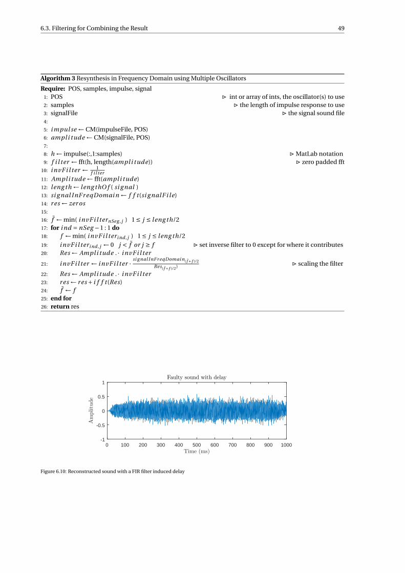
6.3. Filtering for Combining the Result 49
Algorithm 3 Resynthesis in Frequency Domain using Multiple Oscillators
Require: POS, samples, impulse, signal1: POS . int or array of ints, the oscillator(s) to use2: samples . the length of impulse response to use3: signalFile . the signal sound file4:
5: i mpul se ← CM(impulseFile, POS)6: ampli tude ← CM(signalFile, POS)7:
8: h ← impulse(:,1:samples) . MatLab notation9: f i l ter ← fft(h, length(ampli tude)) . zero padded fft
10: i nvF i l ter ← 1f i l ter
11: Ampl i tude ← fft(ampli tude)12: leng th ← leng thO f ( si g nal )13: si g nal InF r eqDomai n ← f f t (si g nalF i le)14: r es ← zer os15:
16: f ← min( i nvF i l ternSeg , j ) 1 ≤ j ≤ leng th/217: for i nd = nSeg −1 : 1 do18: f ← min( i nvF i l teri nd , j ) 1 ≤ j ≤ l eng th/219: i nvF i l teri nd , j ← 0 j < f or j ≥ f . set inverse filter to 0 except for where it contributes20: Res ← Ampl i tude . · i nvF i l ter
21: i nvF i l ter ← i nvF i l ter · si g nal InF r eqDomai n( f + f )/2
Res( f + f )/2) . scaling the filter
22: Res ← Ampl i tude . · i nvF i l ter23: r es ← r es + i f f t (Res)24: f ← f25: end for26: return res
Time (ms)0 100 200 300 400 500 600 700 800 900 1000
Amplitude
-1
-0.5
0
0.5
1
Faulty sound with delay
Figure 6.10: Reconstructed sound with a FIR filter induced delay

50 6. Results and Simulations
frequency in kHz3 4 5 6 7 8 9
Amplitude
0
200
400
600
800
1000
1200
1400
Freq. Content of Result
Figure 6.11: Sound with some frequency gaps
the delay. That is, the sound is filtered once backward. This will introduce a negative delay. The sound is thenfiltered forward and the forward delay will cancel the negative delay from the backward filtering. Becausebackward-forward filters are computationally expensive this is not an optimal solution.
For these reasons it is not practical to filter the resynthesized sound repeatedly in order to combine con-tributions from specific oscillators. A different approach must be used.
6.4. Filtering in the Frequency DomainOne way to circumvent the above filtering complications is to do all the computations strictly in the frequencydomain. This is perfectly viable as long as the entire signal is available at the time of computation.
The filtering that was attempted in the previous section in the time domain is easy in the frequency do-main. That is, the index from the minimum point of the previous contributing inverse filter f up until theindex of the minimum point of the current inverse filter f are the frequencies that the respective inverse filtercontributes to.
Perhaps the most intuitive way to combine the results is to set the unwanted frequencies of the result tozero in the frequency domain prior to the transfer to the time domain. The results from all the oscillators canthen be summed in the time domain to form the final result a.
The smarter approach, however, is to set the values of the inverse filter to zero for the unwanted frequen-cies outside of the range ( f , f ]. This leads directly to a minimization of needed multiplication operations andassignment operations.
6.5. Scaling the ResultAnother important consideration is the scaling of the resulting sound. In a typical time domain wave-form theamplitude should fall in the range −1 ≤ a(t ) ≤ 1. The scaling of the result must be taken into consideration,because when the result does not fall into the stated range then some audio converters will clip audio. Thatis, values a(t ) <−1 are set to −1 and values 1 < a(t ) are set to 1. This is how distortion, also called “clipping”,is introduced.
At the very least, the result must be scaled such that it falls into the −1 ≤ a(t ) ≤ 1 range. This can be doneusing the operation of the following equation:
a(t ) = a(t )
max0≤ti≤t f
(|a(ti )|) (6.1)

6.6. Simulating Hearing Loss 51
Where a is the reconstructed sound and t f is the final time point in aThis is also how incas3 scaled their result (see: Section 4.3). The reason that scaling in this fashion is
inadequate is that to determine the accuracy of a, comparisons of the frequency spectrum of the signal a andthe frequency spectrum of the result a is very helpful. With a poorly scaled a this comparison is challengingbecause the frequency spectrums, given that a is accurate, will be scalar multiples of each other.
A better way to do the scaling is to scale the value max(|a|) to max(|a|), as in Equation 6.2. As long as thetime domain result is very close to that of the signal this method works well.
a(t ) = a(t )
max0≤ti≤t f
(|a(ti )|) max0≤ti≤t f
(|a(ti )|) (6.2)
However, the time representation of the result a is very susceptible to small changes that might not be au-dible to the best of listeners. As soon as there is a small error in the resynthesis, scaling according to Equation6.2 will result in the frequency spectrum of the result a being a scalar multiple of the spectrum of the signala.
The best way to scale the result a is to use the values of the frequency spectrum. For example, to scale thecontribution of a given oscillator, the maximum value of the frequency spectrum, in the part of the spectrumto which the oscillator contributes, is picked. Then, using the ratio of this value from the spectrum of a withthe corresponding value from the spectrum of a to scale a gives the ratio by which a should be amplified. Toimprove robustness, an average of a few sample points from the frequency spectrums of a and a can be usedto derive the amplification ratio.
Because the scaling is linear between the time and frequency domain representations of the same sound,and because the basic operation of the inverse filter when working in the frequency domain is multiplication,the scaling can be applied directly to the inverse filter function. This has a desired effect in two ways. First itreduces the computation of resynthesis after the filter functions have been built. And secondly, it generalizesthe inverse filter function, eliminating the need to compare the amplitude of a with that of a.
It is important to scale the filter function instead of the result. The reason is that the goal is to not justbe able to invert the operation of the cochlea model on a sound input. If this were the goal, then there is noproblem with scaling the resulting sound in comparison with the original sound. But, because the goal is tosimulate damage, the resulting sound is intended to be different from the original sound. Thus, by definitionit is a bad idea to scale the result a to the original signal a.
6.6. Simulating Hearing LossA simple way to simulate hearing loss in the transmission line cochlea model is to update the damping termto have increased damping in the “damage” region. The damping term of the model can be seen in Figure5.14. Of course, the actual damping profile used is as seen in Figure 5.19.
For the damage simulations in this report, the damping term is multiplied with a Gaussian hump (see:Figure 6.12) centered in the cochlea length that affects approximately 10% of the cochlea length. This createsthe theoretical damping profile as seen in Figure 6.13. Of course, the damping profile, with the sponge layer,in actual use is that seen in Figure 6.14.
In Figure 6.15 is a cochleogram of the sound seen in 6.1. In Figure 6.16 is a cochleogram of the same soundsnippet as in Figure 6.15 except here hearing loss is being simulated. There are four lines super-imposed onthis Figure. These four lines correspond to oscillators 250 and 350, plotted in red, and oscillators 282 and319, plotted in green. These lines also correspond with the red and green x’s that are seen in Figure 6.12.That is, the data in the cochleogram that falls between the red lines is in the region affected by the update tothe damping term. The data that falls between the green lines is in the region where the damping term wasmodified to a factor greater than 2.
When comparing Figure 6.15 with Figure 6.16 it can be seen that the wave patterns follow a more vertical(parallel to the Y-axis) orientation in the damage region. This is because sound at the frequency correspond-ing to the damage region will still excite the oscillators, but the oscillations die out much more rapidly dueto the increased damping. Waves on the cochlear partition that start at a higher frequency (lower oscillatornumber) and travel as a wave, along the partition, tend to not have as much of a representation in the damageregion. This is why there is less of the horizontal “drifting” of the wave patterns in the damage region. En-ergy from oscillators prior to the damage region does traverse the region, and will continue to the oscillatorsbeyond the region, however, with less energy than if there was not the damage region.

52 6. Results and Simulations
Oscillator number in the cochlea model0 100 200 300 400 500 600
Factor
1
2
3
4
5
6
7
8
9
10
Guassian Hump
Figure 6.12: Gaussian hump factor used to modify the damping profile of the model, the two red x’s here indicate points where thehump starts and ends. The green x’s indicate the points between which the value will be more than doubled from the normal. On thecochleograms that follow, these values are indicated by similarly colored lines
Oscillator number in the cochlea0 100 200 300 400 500 600
Dam
pingvalue
0
1
2
3
4
5
6
7
8
Damping while simulating damage
Figure 6.13: The theoretical damping profile of a model that simulates hearing loss

6.6. Simulating Hearing Loss 53
Oscillator number in the cochlea0 100 200 300 400 500 600
Dam
pingvalue
0
5
10
15
20
25
Damping while simulating damage
Figure 6.14: The actual damping profile used to simulate hearing loss
Figure 6.15: The cochleogram of “Ten_part.wav”. A cochleogram is a comprehensive visualization of the output from a transmission linecochlea model. On the x-axis is time, on the y-axis the oscillators of the model. On the z-axis is the position of the given oscillator intime.

54 6. Results and Simulations
Figure 6.16: Cochleogram of “Ten_part.wav” while simulating hearing loss. The data that falls between the red lines is in the region wherethe damping term was affected. The data that is between the green lines is the area where the damping was increased beyond a factor of2. The lines corresponding to oscillators 250, 282, 319, and 350 are plotted at a depth of approximately -36.4, -34:9, -35.0, and -32.6 dBrespectively. This is 1.5 dB above the average value of the corresponding oscillator in time. This is also why the super-imposed lines arecovered at some points by the data of the cochleogram.
Figure 6.17: The reconstructed sound sent through a normal hearing model.

6.6. Simulating Hearing Loss 55
Oscillator number in the cochlea model0 100 200 300 400 500 600
Average
respon
selevelin
time
-60
-55
-50
-45
-40
-35
-30
Average of cochleogram per oscillator in time
Original sound
While simulating damage
Response to resynthesized sound
Figure 6.18: Here the time dimension of the cochleograms seen in Figures 6.17, 6.16, and 6.17 is averaged giving a 2-D representation ofthe cochleograms
Using the inverse filters built on the original sound, based on the cochleogram of normal sound (see:Figure 6.15) to resynthesize sound based on the cochleogram that simulates hearing loss (see: Figure 6.16)the resulting sound indeed has much less content in the frequency range corresponding to the damage regionas seen in Figure 6.19. In this figure a deep notch in the frequency content is visible, centered at approximately1.06 kHz.
The resynthesized sound a (not shown) is almost identical to the original a as in Figure 6.1. When thesound a is run through the cochlea model again with the settings on the model set to simulate a healthy earthen a cochleogram almost identical to the one in Figure 6.16 is produced. This cochleogram can be seen inFigure 6.17. These two different cochleograms match very closely.
Just by looking at the Figures 6.16 and 6.17 it is hard to tell how similar, or different, the two cochleogramsare. Therefore, a way to make the comparison easier, is to average the cochleogram in time. In this way the 3-D cochleogram is visualized in 2-D, where the response in time is averaged. In Figure 6.18 three cochleogramsare compared. The cochleogram in Figure 6.15 is a response to the sound a, and is represented by the blueline. Let this model output be denoted by MO1. The cochleogram in Figure 6.16, which is the model output,lets call it MO2, from which the damage sound a is resynthesized from, is represented by the red line. Finally,the cochleogram from Figure 6.17 is represented by the dashed yellow line. This is the cochleogram in re-sponse to the sound a. Let it be denoted by MO3. MO1 and MO2 are very similar up until the damage region,at approximately oscillator 275. Beyond the damage region, the average of MO2 is lower than that of MO1
until about oscillator 500. At this point the two are very similar. Interestingly, the average of MO3 is lower upuntil the middle of the damage area, at oscillator 300. Until oscillator 200 the average is just slightly belowthat of both MO1 and MO2. But it seems that the damage region in a starts a little early with a gap betweenMO2 and MO3 between oscillators 250 and 300. This corresponds to the frequencies higher than the simu-lated damage area, for which, the frequency spectrum plot of the sound a (see: Figure 6.20) showed it wasalmost identical to the original sound a. Because of that, this gap between MO2 and MO3 seems unexpected.Beyond oscillator 300 the average of MO2 and MO3 are almost identical. These results would suggest thatthe resynthesized sound has a slight exaggeration in simulated damage in frequencies just above the damagearea.
The fact that the cochleogram in Figure 6.16, as the result from the model that simulates a damaged earand that the cochleogram seen in Figure 6.17 as the result of the “damaged sound” a on a model of a normalcochlea, are so similar, is strong proof that the sound a is an accurate representation of the damage beingsimulated.

56 6. Results and Simulations
frequency in kHz10
-310
-210
-110
010
110
2
Amplitude
0
200
400
600
800
1000
1200
1400
1600
1800
Freq. Content of Result
Figure 6.19: The frequency content of the sound with simulated hearing loss. The data plotted in blue is the frequency content of theoriginal sound, and the data in orange is the frequency content of the sound with damage being simulated
The main objective of this research project was to be able to produce the sound as a person with hearingloss would hear normal sound. This sound is referred to as a. This objective is met for linear transmissionline cochlea models as evidenced in the previous paragraph. An accurate tool to turn damage that is beingsimulated into sound is hereby provided. Future research that investigates the changes needed in the modelto simulate various kinds of hearing loss could therefore use the tool created here to listen to the effects of thedamage.
6.7. The Damaged SoundIn Figure 6.19 the frequency content of both the original signal as well as the frequency content of the dam-aged sound is seen. “Damaged sound” refers to sound that is the result of simulating hearing loss, or hearingdamage. Let the original sound again be referred to as a, and let a be the sound where hearing loss is sim-ulated. The sound a indeed has less content in the damage region. Careful inspection of Figure 6.19 showsadditional features that are of interest. Zooming in on this figure to the higher frequencies (see Figure 6.20)shows that a is almost identical in the higher frequencies. These frequencies correspond to the oscillatorsthat come before the damage region in the cochlea model. However, inspecting the low frequencies showsthat there is a range of frequencies lower than the damage region in which there is less content than is in theorigional signal. This can be seen in Figure 6.21 in the frequencies in the range of 0.5−0.8 kHz (500−800 Hz).
A plot of the ratio between the frequency content of the sound a to a is shown in Figure 6.22. In thisfigure, it is clearly evident that the ratio between the two is close to 1 for the frequencies higher than thedamage region. At the lowest point the ratio is almost 0.1, which is close to the inverse of the multiple, bywhich the damping term in the model was modified at a factor of 10. In the frequencies below the damageregion, which correspond to the oscillators after the damage region in the model, the ratio tends to be below1, even in the region outside of where damage was simulated. This indicates that by using a transmission linemodel, effects from the damage region propagate to areas not in the damage region. Such propagation ofeffects is not possible when simulating hearing loss through simpler filter bank signal processing.

6.7. The Damaged Sound 57
frequency in kHz10
1
Amplitude
0
200
400
600
800
1000
1200
1400
1600
Freq. Content of Result
Figure 6.20: High frequency content comparison between a and a
frequency in kHz10
-110
0
Amplitude
0
200
400
600
800
1000
1200
1400
1600
1800
Freq. Content of Result
Figure 6.21: Low frequency content comparison between a and a
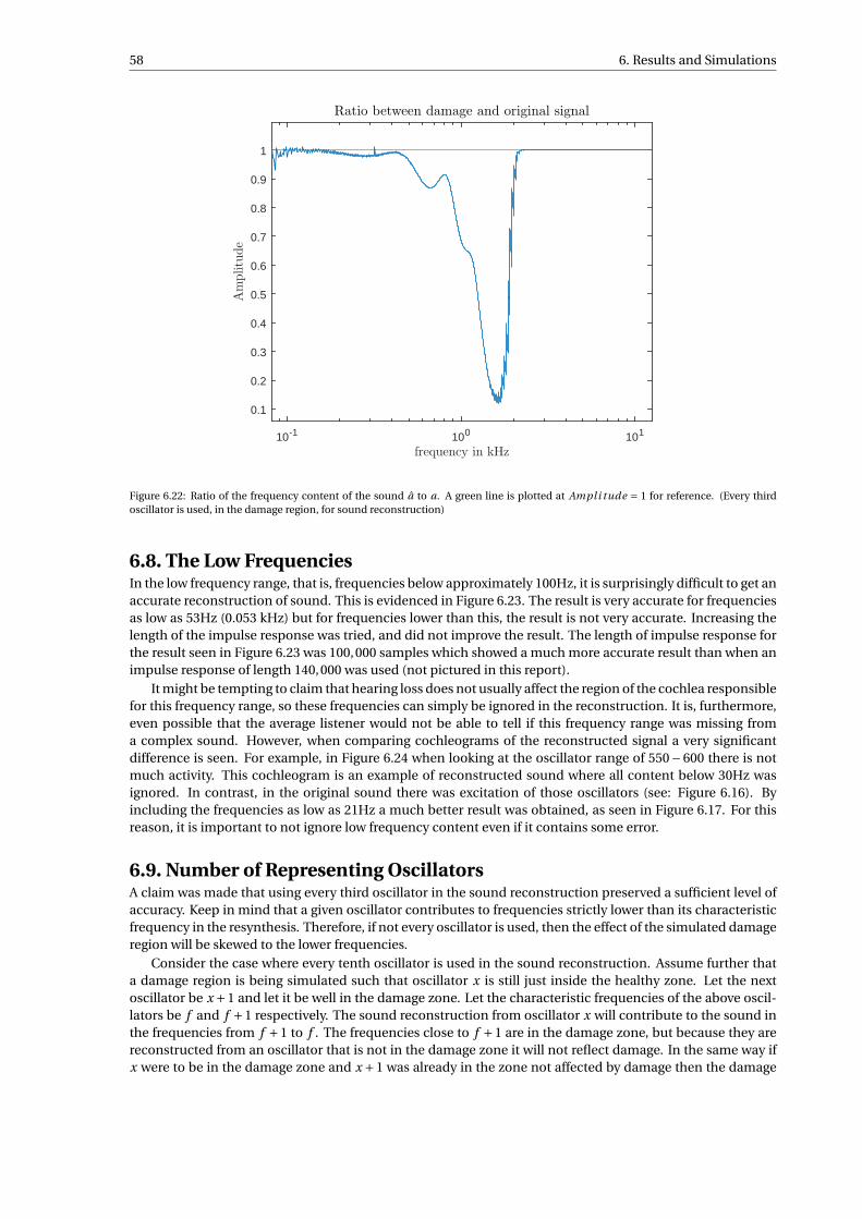
58 6. Results and Simulations
frequency in kHz10
-110
010
1
Amplitude
0.1
0.2
0.3
0.4
0.5
0.6
0.7
0.8
0.9
1
Ratio between damage and original signal
Figure 6.22: Ratio of the frequency content of the sound a to a. A green line is plotted at Ampl i tude = 1 for reference. (Every thirdoscillator is used, in the damage region, for sound reconstruction)
6.8. The Low FrequenciesIn the low frequency range, that is, frequencies below approximately 100Hz, it is surprisingly difficult to get anaccurate reconstruction of sound. This is evidenced in Figure 6.23. The result is very accurate for frequenciesas low as 53Hz (0.053 kHz) but for frequencies lower than this, the result is not very accurate. Increasing thelength of the impulse response was tried, and did not improve the result. The length of impulse response forthe result seen in Figure 6.23 was 100,000 samples which showed a much more accurate result than when animpulse response of length 140,000 was used (not pictured in this report).
It might be tempting to claim that hearing loss does not usually affect the region of the cochlea responsiblefor this frequency range, so these frequencies can simply be ignored in the reconstruction. It is, furthermore,even possible that the average listener would not be able to tell if this frequency range was missing froma complex sound. However, when comparing cochleograms of the reconstructed signal a very significantdifference is seen. For example, in Figure 6.24 when looking at the oscillator range of 550−600 there is notmuch activity. This cochleogram is an example of reconstructed sound where all content below 30Hz wasignored. In contrast, in the original sound there was excitation of those oscillators (see: Figure 6.16). Byincluding the frequencies as low as 21Hz a much better result was obtained, as seen in Figure 6.17. For thisreason, it is important to not ignore low frequency content even if it contains some error.
6.9. Number of Representing OscillatorsA claim was made that using every third oscillator in the sound reconstruction preserved a sufficient level ofaccuracy. Keep in mind that a given oscillator contributes to frequencies strictly lower than its characteristicfrequency in the resynthesis. Therefore, if not every oscillator is used, then the effect of the simulated damageregion will be skewed to the lower frequencies.
Consider the case where every tenth oscillator is used in the sound reconstruction. Assume further thata damage region is being simulated such that oscillator x is still just inside the healthy zone. Let the nextoscillator be x +1 and let it be well in the damage zone. Let the characteristic frequencies of the above oscil-lators be f and f +1 respectively. The sound reconstruction from oscillator x will contribute to the sound inthe frequencies from f +1 to f . The frequencies close to f +1 are in the damage zone, but because they arereconstructed from an oscillator that is not in the damage zone it will not reflect damage. In the same way ifx were to be in the damage zone and x +1 was already in the zone not affected by damage then the damage

6.9. Number of Representing Oscillators 59
frequency in kHz0.02 0.04 0.06 0.08 0.1 0.12 0.14
Amplitude
0
50
100
150
200
250
300
350
Freq. Content of Result
Original Signal
Result Signal
Figure 6.23: Error of the reconstructed (result) sound in the low frequencies
Figure 6.24: Cochleogram of sound reconstructed where sound content bellow 30 Hz was ignored. This can be seen in the oscillatorrange above 550

60 6. Results and Simulations
frequency in kHz10
-110
010
1
Amplitude
0.1
0.2
0.3
0.4
0.5
0.6
0.7
0.8
0.9
1
Ratio between damage and original signal
Figure 6.25: The ratio between the frequency spectrum content of the original sound a and the damage sound a where every oscillatoris used in the damage region
would be projected into a frequency range where there is not to be damage.This effect is present, and it is visible when carefully observing the frequency spectrums of the resultant
damage sound. To see the improvement of using every oscillator versus using every third oscillator compareFigure 6.22, where every third oscillator is used, and Figure 6.25, where every oscillator is used. On the highfrequency side of the damage notch, the ratio is clearly smoother with a denser oscillator concentration.Strangely, when comparing the cochleograms there was not a clear improvement by using more oscillatorsversus using fewer.

7Conclusion
7.1. DiscussionHearing loss is a significant global health problem of increasing prevalence. For those that suffer from it, itgreatly decreases the quality of life. As such, research in this area will become more important in the com-ing years. A facet of this research will be the development of high quality hearing loss simulators. These areneeded, both for educational purposes, and also to aid in the faster and more cost effective development oftreatment for hearing loss. Because the human auditory system is amazingly complex, hearing loss simula-tors need to take as many physical phenomena into account as possible.
A practitioner in the field of hearing simulation must have a working knowledge of the human auditorysystem. In this report the needed groundwork, as it relates to hearing loss, is clearly and concisely presented.The transmission line cochlea model, also, is elaborated on and explained. Digital signal processing, an in-dispensable ingredient of simulating hearing loss, is also introduced.
This research project contributes to the goal of simulating hearing loss in a few ways. Firstly, the methodsto simulate hearing loss are based on a mathematical model of the ear. This allows for more physical phe-nomena of hearing loss to be accounted for than do filter bank methods. To make the simulation of hearingloss, by use of the transmission line cochlea model, possible for the first time, a variety of problems are suc-cessfully dealt with. For the simulations to work, residual energy in the model needs to be dealt with properly.As long as this is not done, sound resynthesis could only be done for exceedingly short sound inputs, and onlyusing a small part of the oscillators representing the cochlea. Hearing loss simulations would fail to be real-ized because a greater part of the cochlea must be represented. Furthermore, a technique to combine thecontributions from multiple oscillators is developed, such that accurate sound can be reproduced from themodel output. The resulting sound is accurate, both in time and frequency domain representations.
Using the developed methods for sound resynthesis to simulate hearing loss shows promise because un-like for filter bank methods, the effects of damage in one area of the cochlea propagates to other areas ofthe cochlea. Furthermore, the cochleogram from the model that simulated damage looks very similar to thecochleogram of a normal cochlea in response to the resynthesized damage sound. This demonstrates thatthe sound that is resynthesized accurately represents the damage that the model simulates.
7.2. RecommendationsThis project lays the groundwork for a few areas of further research. Many of the hearing phenomena in thehuman auditory system are nonlinear. There are also nonlinear transmission line cochlea models. Hence,an important topic for further research would be to extend the back transformation methods developed inthis project for linear models to work for nonlinear models. A good starting point would be to use linearinverse filters on nonlinear output. The time segments should be kept as short as possible. Each inverse filterwould need to be individually scaled for each time segment of sound by comparing the result of normallyresynthesized sound with the original input sound. To simulate damage, an inversely scaled filter should beused.
To simulate damage, the damping term of the cochlea is modified. Another needed research area, is toinvestigate the optimal levels and methods of modifying the damping term to simulate various known typesof hearing loss. There is an abundance of literature on psychoacoustics (psychoacoustics is the study of sound
61

62 7. Conclusion
perception) that could be used to calibrate the modifications of the damping term. This type of research isrequired to make hearing loss simulations, based on the transmission line cochlea model, a useful tool to thehearing industry.
A third area for further research relates to the method of negating the build-up of residual energy in thecochlea model. In the current project, a sponge layer of increased damping is used. Further research shouldanswer if this is indeed the best way to handle residual energy. If so, what is the optimal application of thistechnique to match the conditions in the human cochlea. Further research should also investigate if energyreflection and the buildup of residual energy is also a problem in nonlinear transmission line cochlea models.
7.3. The EndFor the first time sound has been successfully and accurately resynthesized from a linear transmission linecochlea model output. Such output has been analyzed by the use of cochleograms in the past. Resynthesizedsound introduces a new way of exploring the output of such models. But, more importantly, a new methodto simulate hearing loss hereby came into existence.

AMatLab Code for Sound Resynthesis
MatLab code for the resynthesis algorithm. This code follows Algorithm 3 from Section 6.2.
% The code in this file computes inverse filters to do soundresynthisis
% from the output of a transmission line cochlea model (CM). To get theCM
% output it will either need to be used in conjuntion with the function% cochleogram_dimensionless_RK4_func.m or the CM output will need to be% uploaded into memory such that the MatLab workspace can access the
needed% variables.% This file is based on functions provided by INCAS3
% Let us begin:% Clear MatLab command screen and displaying progress messageclc;disp('Working on it');disp('-------------------------------------------')
%% Runtime Parameters:% The current code assumes the CM uses 600 OsillatorsPOS = 1:600; % the oscillators to get traces forpos = 1:60; % the (subset of) oscillators to use for sound
reconstruction
SIM_LOSS = true; % Set to true to use the contributionsfrom multiple oscillators
samples = 100000; % Length of impulse response to use forreconstruction
GRAPH = true; % Plot the original sound and thereconstruction?
SOUNDORIG = false; % Playback the original sound beforeplaying back the reconstruction
SOUND = false; % Playback the reconstructed soundgetFilter = true; % Set to true if the filter function are to
be computedgetTrace = true; % Set to true if traces need to be made
with the cochlea modelCUTOFFdB = 140; % The dB bound for the inverse filter
functions
63

64 A. MatLab Code for Sound Resynthesis
% Directry where sound files to be processed areWorkingDir = 'C:\ Users\Leo\Dropbox\MastersProgram\Thesis\
SimpleSoundFiles\';% name of the signal to processfileNameSignal = 'DamageSimSparseOsc.wav';% name of sound file if the sound is to be saved , leave blank if file
should not be savedfilenameRes = [];% If loading amplitude from a .mat fileampMatFile = 'NormHearLin10Part1Sec ';
%% Getting the impulse response and the oscillator trace from soundinput
if getTracedisp('Getting oscillator trace of impulse ');disp('-------------------------------------------')
% Building the impulse "Sound signal"t = zeros(1,samples);t(1) = 1;
% Getting the impulse response of the system[impulse , cm_sRate] = cochleogram_dimensionless_RK4_func(t,POS);
% resampling the sound signal to the sample rate of the CMdisp('Getting oscillator trace of sound')disp('-------------------------------------------')[signal ,signal_sf] = audioread ([ WorkingDir fileNameSignal ]);
% Resampling is done in two steps , the ratio can be too large for asingle step
% Doing it in two steps is also more memory efficientif cm_sRate ~= signal_sf
signal_cm_sRate = resample(signal , cm_sRate ,signal_sf);signal_2cm_sRate = resample(signal_cm_sRate , 2 ,1);
end
fprintf('Signal resampled from %i sRate to %i 2* cm_sRate\n',signal_sf , 2* cm_sRate);
% Getting the oscillator traces for the singal sound file[amplitude , cm_sRate] = cochleogram_dimensionless_RK4_func(
signal_2cm_sRate ,POS);end
% Uncomment this line to stop the program here and allow to save thevariables
% generated up until this point for future use
%return;
if ~exist('amplitude ')disp('Load a valid oscillator trace or set getTrace = true')

65
return;end
% Setting signal length and number oscillator traces to compute fornSeg = length(pos);ampLength = length(amplitude);
%% Computing the inverse filter; this was originally a separate filecalled get filter
if getFilterdisp('Calculating tuning curves ')disp('-------------------------------------------')
if ~exist('impulse ', 'var')disp('Load a valid impulse file');
return;end
% Getting the length of impulse response to be used for inversefilter
h = impulse(pos ,1: samples);
% Making the tuning curvesf = fft(h, ampLength , 2);
% Bounding the inverse filters to decrease error amplificationm = max (20 * log10(abs(f)) ,[],2) * ones(1, ampLength);
% set f to 1 where it is zero to avoid divide by zero errorf = f + (f==0);
% computing the bound to eliminate error peaksb = (20 * log10(abs(f)) > (m - CUTOFFdB));
% All values of the tuning curve below CUTTOFFdB less than the peakare
% set to the value of boundbound = (10 .^ ((m - CUTOFFdB)/20));
% the indices of f were b == 1 are set to boundf = (b .* f) + (~b .* bound);
disp('Calculating inverse filter functions ')disp('-------------------------------------------')
% Inverting the tuning curve to create the invers filterinv_f = 1./f;fAmpl = fft(amplitude ,[],2);
end
fax_Hz = (0: ampLength -1)*cm_sRate /( ampLength);fax_kHz = fax_Hz /1000;
res = zeros(1, ampLength);

66 A. MatLab Code for Sound Resynthesis
% This is the old way of combining the contributions used by INCAS3if ~SIM_LOSS
disp('Calculating results ')disp('-------------------------------------------')Res = zeros(1, ampLength);
% combining the result of the different segments in the frequencydomain
for seg = 1:nSegRes = Res + fAmpl(seg ,:) .* inv_f(seg ,:);%(2:end);
end
res = real(ifft(Res)); % transferring the result in the frequencydomain to the time domain
% scaling the result in the time domainres = res / ( 1/max(abs(signal)) * max(abs(res (10000:end -10000)))
);
else % The modified method of combining the results
disp('Calculating results ')disp('-------------------------------------------')% Finding the charachteristic freq. of the segmentfax_Hz = (0: ampLength -1)*cm_sRate / ampLength;fax_kHz = fax_Hz /1000;
% boolean to control the low frequency reconstructionfirstFilter = true;
% \tilde f in the report , the lower bound that the specific filteris
% to contribute to[M,oldI] = min(abs(inv_f(nSeg ,1: floor(end/2))));
% The first filter is not actually usedinv_f(nSeg ,:) = zeros(size(inv_f(nSeg ,:)));
% The number of iterations of scaling the inverse filter to usescaleIter = 5;
% Combining the resultsfor ind = nSeg -1: -1:1
% Print the progress every 10 segmentsif rem( ind , 10 ) == 0;
fprintf('Remaining steps: %d \n', ind );end
% unless the filter has already been built and should no longerbe touched
if getFilter
[M,I] = min(abs(inv_f(ind ,1: floor(end/2))));
if (oldI + 2) >= I % A filter needs to contribute to atleast two frequency points

67
inv_f(ind ,:) = zeros(size(inv_f(ind ,:)));continue;
end
if firstFilter % if first filter then set everything below21 Hz to zeroinv_f(ind ,1:20) = zeros (1,20); % Getting rid of low
freq. errorinv_f(ind , I+1:end) = zeros(1,ampLength -I);firstFilter = false; % so there is only one first
filterelseif ind == 1 % if this is the last filter then set
frequencies above 30 kHz to zeroinv_f(ind , 1:oldI) = zeros(1,oldI);inv_f(ind , 30000: end) = zeros(1,ampLength -30000+1);
% otherwise set the filter to zero except in the frequencyranges that it contributes to sound reconstruction
elseinv_f(ind , 1:oldI) = zeros(1,oldI);inv_f(ind , I+1:end) = zeros(1,ampLength -I);
end
if I - oldI < 22pfas = floor((I - oldI)/2) -1; % think sample points to
use in the averageelse
pfas = 10; % think sample points to use in the averageend
% Used to get the ratio by which to scale the inversefilters
freqContSignal = abs(fft(signal_cm_sRate '));avgStartInd = floor ((oldI+I)/2-pfas);if avgStartInd < 21
avgStartInd = 21;endavgEndInd = floor ((oldI+I)/2+ pfas);avgSign = mean( freqContSignal(avgStartInd:avgEndInd));
% A few iterations of scaling the inverse filterfor scalling = 1: scaleIter
Res = fAmpl(ind ,:) .* inv_f(ind ,:);tempRes = real(ifft(Res));freqContRes = abs(fft(tempRes));avgRes = mean( freqContRes( avgStartInd:avgEndInd) );if scalling ~= scaleIter
inv_f(ind ,:) = inv_f(ind ,:)*( avgSign/avgRes);end
end
% Constructing the time domain signalres = res + tempRes;
else % The filters have already been built just construct theresult

68 A. MatLab Code for Sound Resynthesis
if max(abs(inv_f(ind ,1: floor(end/2)))) > 1Res = fAmpl(ind ,:) .* inv_f(ind ,:);tempRes = real(ifft(Res));res = res + tempRes;
endend
oldI = I;
if GRAPHfigure (3)plot(res);title('3', 'Interpreter ','latex');drawnow;
endend
end
disp('Calculations Done')disp('-------------------------------------------')
foi = 30000;
%% Now the work is done the rest is just outputs and cleanup
% Plot graphs for report or the origional sound file with thereconstructed
% sound fileif GRAPH
% plotting original sound and reconstructed soundfigure (10)subplot (2,1,1)plot ([0: ampLength -1]/( cm_sRate /1000) , signal_cm_sRate)subplot (2,1,2)plot(res)
end
res_sf = (( length(res))/ampLength) * signal_sf;
% Playing the original soundif SOUNDORIG
sound(signal , res_sf);pause (18);
end
% Playing the reconstructed soundif SOUND
soundToPlay = resample(res ,signal_sf ,cm_sRate);sound(soundToPlay , signal_sf);
end
% write the reconstruction to a wav fileif ~isempty(filenameRes)
soundToPlay = resample(res ,signal_sf ,cm_sRate);audiowrite ([ filenameRes '.wav'], soundToPlay , signal_sf);
end

BMatLab Code for the Updated Cochlea
Model
MatLab code for the updated transmission line cochlea model. This code is set as a function with returnvariables. It also includes settings to allow for the sponge layer to be turned on and off. The sponge layer is asdescribed in Section 5.4.2. It also allows for hearing loss to be simulated by updating the damping term.
% This implementation of the dimensionless Cochlea model followed the% 16/1/1991 document by Marc van den Raadt as closely as possible.%% 19/3/2013: Added Zweig impedance infrastructure.% This follows the FORTRAN 77 code (from INCAS3) as closely as possible
.%% 10/20/2015: Added Sponge layer at the helicotrema and allows for the% simulation of hearing loss by updating the damping term. It also is% set as a function rather than a script. Furthermore , it is modified
to% accept an arbitrary sound file as either a path to a file , or as a% numeric array% - Leo Koop , Simulating Hearing Loss , October 20, 2015%%% Author: Jan Stegenga% Version: 0% Date: 1/2/2013% Copyright: INCAS3 , The Netherlands%% The changes to linear version validated on 06/09/2015 (Leo)%
function [ pos_trace , cm_sRate ] = cochleogram_dimensionless_RK4_func(filename , POS )
% INPUT: filename -- is the sound file to pass into the cochlea% POS -- is the oscillator to get the trace of
place_map = 'fortran ';LINEAR = 1;ZWEIG = 0;TIMESTEP = 200;PLOT = 0;
69

70 B. MatLab Code for the Updated Cochlea Model
KILL_ENERGY = 1; % Set to '1' or true to add the spongelayer
SIMULATE_DAMAGE = 0; % Set to '1' or true to modify thedamping term to simulate damage
VSOM_CORR = 1;% parameter list found on page A4 (van den Raadt [3])% some parameters are explained on pages A1 to A3
% number of segments (oscillators) (excluding the midear andhelicotrema)
N = 600;% [s] simulation time stepdt = 2.0e-6;% [s] time reference , used to normalize the timet_0_hat = 1e-3;% [m] length reference (x), used to normalize BM lengthx_0_hat = 35e-3;% [m] amplitude reference ,% used to normalize dynamic values of amplitude and amplitude
changey_0_hat = 1e-9;% [m] width scalae (page 19)b = 1e-3;% BM width as function of segment (index) = scalae widthb_BM = b*ones(N,1);% [m] height of scalae (page 3)h = 1e-3;% [m^2] cross sectional area of the cochlea = b*hs_sc = 1e-6;% [kg/m^3] density of cochlear fluidrho = 1e3;% [kg/m^3] specifiek acoustic mass of BMm_s = 0.5;% [m^2] area of a segment (stape)s_st = 3e-6;% [m^2] area of eardrums_t = 60e-6;% [rad/s] resonance frequency of midearomega_rm = 2*pi *2000;% Reciprocal of the Q factor of the mideardelta = 2.5;% Transformationfactor of the midearn_t = 30;% [Ns/m^3] Specific acoustic impedance of airZ_s = 415;% Parameter created by normalization on xalpha_squared = 4900;% Parameter created by normalization on xalpha_x_squared= alpha_squared;% [Pa] reference pressure , equals 0 dB SPLp_ref = 2e-5;% [Pa/m] constant for specific acoustic stiffnesss_0 = 1e10;% [/m] determines relationship between frequency and location
(x)

71
lambda = 300;% modulation factor for the impulse response of a resonatorepsilon = 5e-2;% normalized midear segment (stape) lengthdx_01_tilde = 1/N;% demping at the helicotrema , according to the fortran code:dhel = 2.2e7;
if place_map == 'fortran '% normalized stape length , following the f77 versiondx_tilde = (1-dx_01_tilde -(h/x_0_hat))/N;% definition x_tildex_tilde_v = [ 0, dx_01_tilde : dx_tilde : 1 - h/x_0_hat -
dx_tilde ];% x_tilde has to be a column vectorx_tilde = x_tilde_v (:);
else% normalized stape length , following Van den Raadtdx_tilde = 1/N;x_tilde_v = 0: dx_tilde :1;% x_tilde has to be a column vectorx_tilde = x_tilde_v (:);
end
% parameters for the nonlinear part of the damping , page 34mu_p1_tilde = 1; % == chi_tildemu_p2_tilde = 1; % == alhpa_tildemu_n1_tilde = 2; % == 2* gamma_tildemu_n2_tilde = 1; % == beta_tilde (or B_tilde)
lambda_tilde = lambda*x_0_hat;% page 33
gamma = m_s * s_t * omega_rm * delta / ( b * x_0_hat *dx_tilde * n_t^2 * Z_s );
% page 27, b_BM replaced by balpha_0 = gamma .* alpha_squared * dx_tilde;
% page 27alpha_x_squared= 2*rho*b_BM (1: end) * x_0_hat ^2 / ( m_s * s_sc );
% page 27
y_tilde = zeros( N+1, 1 ); % page A3 , volume displacementof BM
u_tilde = zeros( N+1, 1 ); % page A3 , volume velocity ofBM
phi_tilde = zeros( N+1, 1 ); % page 16, dimensionless phi ,% phi = pressure/specific mass , phi replaces accelaration in p = m*
a
% page 21, specific acoustic massm_sm = ( n_t^2 * Z_s * s_st ) / ( s_t * omega_rm * delta );% page 6 and 7, g = damping * u + stiffness * y ->% du/dt = 1/m*( p-g ), with g is dimensionless Gg = zeros( N+1, 1 );% page 25, A*phi_tilde = r; where r is represents the next state of

72 B. MatLab Code for the Updated Cochlea Model
% uncoupled oscillators and A is the relation between neighbouringoscillators
r = zeros( N+1, 1 );
% stimulus parameters% page 22, pure tone input: p_e = p_AM1*omega_1*cos( 2*pi*f_1*t )
)p_AM1 = p_ref *10^(60/20); % [Pa] stimulus: 60
dBomega_1 = 1; % parameter to smooth -start the signalf_1 = 1000; % [Hz]
% dimensionless A construction % page 26% N+1 diagonal elementsA = diag( [ - ( 1 + alpha_0 * dx_01_tilde ); ...- (2+ alpha_x_squared (1:N-1) * dx_tilde ^2 ); ...- (1+ alpha_x_squared(N)*dx_tilde ^2+(4* x_0_hat*dx_tilde)/(pi*h+4*
x_0_hat*dx_tilde)) ], 0 );
% Impedance matching at the helicotrema , according to the fortrancode
A = diag( [ - ( 1 + alpha_0 * dx_01_tilde ); ...- (2+ alpha_x_squared (1:N-1) * dx_tilde ^2 ); ...- (2+ alpha_x_squared (1) * dx_tilde ^2 -1. + (1.69e5/ (1.69 e5 +8.26161
e5))) ],0); ...%- (1+ alpha_x_squared(N)*dx_tilde ^2+(4* x_0_hat*dx_tilde)/(pi*h+4*
x_0_hat*dx_tilde)) ], 0 );
% add N above -diagonal elementsA = A + diag( ones(N, 1), 1 );% add N below -diagonal elementsA = A + diag( ones(N, 1), -1 );% invA is easiest way to solve the equation on page 26invA = inv(A);
%% Pure Tone input that came with the file%{% input constructiont = 0:dt:0.1; % timet_tilde = t/t_0_hat; % normalized
timedt_tilde = dt/t_0_hat; % normalized
timestepp_e = p_AM1*omega_1*sin( 2*pi*f_1*t_0_hat*t_tilde ); %0.1*
p_AM1*randn(size(t)) +% is in fact in the unscaled time domain , since t = t_0_hat *
t_tildetaper = exp(-(4- t_tilde).^2); % taper , as used in the
FORTRAN code.% It prevents startup spurious eventstaper(t_tilde >4) = 1; % taperP_e = ( t_0_hat ^2/ y_0_hat )*( n_t * p_e / m_s ).* taper;% is scaled in time and amplitude%}% END of Pure Tone input that came with the file%% From file or array input construction

73
dt_tilde = dt/t_0_hat; % normalizedtimestep
% Modifications by Leo to allow for the input of arbitrarysound files or
% sound represented as a numerical arrayif(isa(filename , 'char'))
[P_e , sRate] = audioread(filename);elseif (isa(filename , 'double '))
P_e = filename;sRate = 2*ceil (1/dt);
end
time_in_seconds = length(P_e)/sRate;
% A few modifications to save some memory since t_tilde wasused only for
% the printing of the title of the plot at the end of thefunction
% t = 0:dt:time_in_seconds; % time% t_tilde = t/t_0_hat; %
normalized time%using the following instead of the above to try and save
memoryt_tilde = 0:dt:time_in_seconds; % timedt_tilde = dt/t_0_hat; %
normalized time
% Resampling the sound filecm_sRate = ceil (1/dt);% I am pretty sure this should be just 1/dt
instead of cm_sRate = ceil (1/( t_0_hat*dt));if 2* cm_sRate ~= sRate
P_e = resample(P_e , 2* cm_sRate ,sRate);end%END From file or array input construction
% Zweig impedance initialization , uses precomputed d and sd1 = - 0.12; % = aplha (in FORTRAN 77 code)d2 = 0.01; % = betad3 = 0.062; % = gammad4 = 0.1416; % = delta
if ZWEIGd1 = d1+(epsilon -d1).*(exp( -20.* x_tilde (2: end))+exp( -20.*(1-
x_tilde (2:end))));% modification to make the model more stable , FORTRANd4 = d4.*(1-exp (-20.* x_tilde (2:end))-exp (-20.*(1 - x_tilde (2: end)
)));% modification to make the model more stable , FORTRAN
end
if LINEARd_prof = 1; %d1;c_prof = 1; %d4;

74 B. MatLab Code for the Updated Cochlea Model
end
% LEO EDIT: This is the damping profile of the code that I received% Van den Raadtd = epsilon*t_0_hat*sqrt(s_0/m_s)*exp( -0.5* lambda_tilde .* x_tilde (2:
end));s = t_0_hat ^2 / m_s * s_0 .*exp( - lambda_tilde .* x_tilde (2:end) )
;
% LEO EDIT: This is what I changedif KILL_ENERGY && LINEAR % So I can turn off my
changes
% currently the sponge layer is only tested to work for thelinear version of the code
x_temp = linspace (0 ,1,600);
% This is the change to d(x)d = d.*(1+560* exp(-25*(1- x_temp)))';
end
% If damage is to be simulated the damping term is updated inthe following lines
if SIMULATE_DAMAGE
damage = gausswin (600 ,35); % Centered Guassian humpaffecting approx 10% of width
damage = 1 + 9* damage;
% figure (2)% plot (1:600 , damage , 'b')% title('Guassian Hump ','Interpreter ','latex ')% xlabel('Oscillator number in the cochlea model ', 'Interpreter
','latex ')% ylabel('Factor ', 'Interpreter ','latex ')% axis ([0 600 0.5 10.5])% hold on% plot (250, 1, 'rx ', 350, 1, 'rx ', 282, 1, 'gx ', 319, 1, 'gx ')
% return;% d = d.* damage; % updating the damping to reflect the damage
% figure (3)% plot (1:600 , d)% title('Damping while simulating damage ','Interpreter ','latex ')% xlabel('Oscillator number in the cochlea ', 'Interpreter ','
latex ')% ylabel('Damping value ', 'Interpreter ','latex ')
end
if ZWEIG% implementation optimized for octave:d = d./ epsilon;% resonance frequency of elements

75
freq = sqrt( s./ t_0_hat ^2 )/2/pi;% formula in Zweig 's article; gives the delays required in
Zweig 's feedbackper = 1.75./( freq*dt );% roundoff; gives the length of shift register per elementn_per = floor( per + 1 );% per gives the percentage needed to approximate contribution
if% delay(i) is not integer number of sample timesper = n_per - per;per = per (:);n_per = n_per (:);% gives much used indexes into ybuf array (a.o. edges of shift
registers)cumsum_n_per = cumsum( n_per );% all N shift registers are in a single column arrayybuf = zeros( sum(n_per), 1, 'double ' ); % In
matlab this needs to be changed 'double 'end
% yter is used for the Zweig -related update and is not in the vanden Raadt document
yter = zeros( N, 1);
u_tilde_log = zeros(N+1, 1);
pos_trace = zeros(length(POS), ceil(length(P_e)/2));% loop through the simulationif PLOT
figure (1);endtimestep_last = length(P_e) -2;
% LEO EDIT:% Modifications were made to allow for arbitrary sound input% one change is to iterate over the sound file every two sample
points% make sure that the sound file has a sample rate 2 times that of
the% sample rate of the cochlea model% Every 2nd sample point is used as the half step for the RK4
method% The updates to accept arbitrary input was benchmarked for the
linear version% but not specifically for the non -linear version of the modelfor timestep = 1:2: timestep_last
% LEO EDIT% Print a progress reportif rem( timestep , 10000 ) <=1;
fprintf('This is timestep: %d of %d \n', timestep ,timestep_last);
end
% compute Zweig update and shift the corresponding registers;% implementation for octave optimality; see FORTRAN code

76 B. MatLab Code for the Updated Cochlea Model
if ZWEIG% weighted update of yter; the feedback termyter = per.*ybuf( -1 + cumsum_n_per ) + (1 - per).*
ybuf( cumsum_n_per );% shift register: ybuf(i) = ybuf(i-1), shift (..) is very
slowybuf = [0; ybuf (1:end -1)]; % WAITING FOR
CONFIRMATION ON THIS% insert new values at 'edges ' of shift registersybuf( cumsum_n_per - n_per + 1 ) = y_tilde( 2:end );
end
%compute the nonlinearity contributionsif ~LINEAR
% nonlinearities as in FORTRAN 77d_prof = dnl( u_tilde (2: end)/100, d1 , d2, d3 );c_prof = cnl( u_tilde (2: end)/100, d2 , d4 );
end
% NOTE: For now if using NL then do not use ZWEIGif ZWEIG
d_prof = d1;c_prof = d4;
end
% compute g% g_0 on page 24; 0 u_tilde (1) = u_0_tilde , y_tilde (1) =
y_0_tilde% g_i on page 36, part with yter is only in FORTRAN 77 code;
yter will% remain zerog = [ (n_t ^2*Z_s/m_s)*(s_st/s_t)*( t_0_hat*u_tilde (1)+omega_rm/
delta*t_0_hat ^2* y_tilde (1)); ...d_prof .*d.* u_tilde (2: end)+s.* y_tilde (2:end)+c_prof .*s.*
yter ];
% compute r% page 26; r_0 = r(1) ; g(1) = g_0r = [ - alpha_0*dx_01_tilde *(P_e(timestep) + g(1)); ...
- alpha_x_squared .* dx_tilde ^2.*g(2:end) ];% Some modification in the FORTRAN coder(2) = r(2)*dx_01_tilde/dx_tilde;if VSOM_CORR
Vsom = sum(u_tilde (2: end));Vsom = Vsom * dx_tilde * x_0_hat * b;r(end) = r(end) + (t_0_hat*dhel/m_s)*(-1.* s_st*u_tilde (1)-
Vsom);end
% solve A * phi_tilde = r % page 25phi_tilde = invA * r;
% Fourth -order Runge -Kutta method% (Diependaal , Duifhuis , Hoogstraten , Viergever [2]).% In this code: u(t) = y(t), v(t) = u(t) and omega[t, y(t), u(t
)] =

77
% [ ( m_s / m_sm )*( phi_tilde (1) - g(1) - P_e(timestep) );% phi_tilde (2: end) - g(2: end) ].functie1 = [ ( m_s / m_sm )*( phi_tilde (1) - g(1) - P_e(
timestep) );phi_tilde (2: end) - g(2:end) ];
y_tilde1 = y_tilde + 0.5* dt_tilde *u_tilde;u_tilde1 = u_tilde + 0.5* dt_tilde *( functie1 );
% Determine g (again)
g = [ (n_t ^2*Z_s/m_s)*(s_st/s_t)*( t_0_hat*u_tilde1 (1)+omega_rm/delta*t_0_hat ^2* y_tilde1 (1)); ...
d_prof .*d.* u_tilde1 (2: end)+s.* y_tilde1 (2: end)+c_prof .*s.*yter ];
% Determine p_e (t + 0.5*dt)%%% p_e = p_AM1*omega_1*sin (2*pi*f_1*t_0_hat *( t_tilde +0.5*
dt_tilde)); %0.1* p_AM1*randn(size(t))+%%% P_e = ( t_0_hat ^2/ y_0_hat )*( n_t * p_e / m_s ).* taper;
% Determine r (again)r = [ - alpha_0*dx_01_tilde *( P_e(timestep + 1) + g(1) ) ;
... % EDIT By LEO- alpha_x_squared .* dx_tilde ^2.*g(2:end) ];
r(2) = r(2)*dx_01_tilde/dx_tilde;
if VSOM_CORRVsom = sum(u_tilde1 (2: end));Vsom = Vsom * dx_tilde * x_0_hat * b;r(end) = r(end) + (t_0_hat*dhel/m_s)*(-1.* s_st*u_tilde1 (1)-
Vsom);end% Calculate phi_tildephi_tilde = invA * r;
functie2 = [ ( m_s / m_sm )*( phi_tilde (1) - g(1) - P_e(timestep + 1) );phi_tilde (2: end) - g(2:end) ];
y_tilde2 = y_tilde + 0.5* dt_tilde*u_tilde1;u_tilde2 = u_tilde + 0.5* dt_tilde *( functie2 );
% Repeat this for g, r and phi_tildeg = [ (n_t ^2*Z_s/m_s)*(s_st/s_t)*( t_0_hat*u_tilde2 (1)+omega_rm/
delta*t_0_hat ^2* y_tilde2 (1)); ...d_prof .*d.* u_tilde2 (2: end)+s.* y_tilde2 (2: end)+c_prof .*s
.*yter ];r = [ - alpha_0*dx_01_tilde *( P_e(timestep + 1) + g(1) ) ;
... % EDIT By LEO- alpha_x_squared .* dx_tilde ^2.*g(2:end) ];
r(2) = r(2)*dx_01_tilde/dx_tilde;
if VSOM_CORRVsom = sum(u_tilde2 (2: end));Vsom = Vsom * dx_tilde * x_0_hat * b;r(end) = r(end) + (t_0_hat*dhel/m_s)*(-1.* s_st*u_tilde2 (1)-
Vsom);endphi_tilde = invA * r;

78 B. MatLab Code for the Updated Cochlea Model
functie3 = [ ( m_s / m_sm )*( phi_tilde (1) - g(1) - P_e(timestep + 1) ); % EDIT By LEOphi_tilde (2: end) - g(2:end) ];
y_tilde3 = y_tilde + dt_tilde*u_tilde2;u_tilde3 = u_tilde + dt_tilde *( functie3 );
% Determine p_e again (t + dt)%%% p_e = p_AM1*omega_1*sin (2*pi*f_1*t_0_hat *( t_tilde+dt_tilde)
); %0.1* p_AM1*randn(size(t))+%%% P_e = ( t_0_hat ^2/ y_0_hat )*( n_t * p_e / m_s ).* taper;
g = [ (n_t ^2*Z_s/m_s)*(s_st/s_t)*( t_0_hat*u_tilde3 (1)+omega_rm/delta*t_0_hat ^2* y_tilde3 (1)); ...
d_prof .*d.* u_tilde3 (2: end)+s.* y_tilde3 (2: end)+c_prof .*s.*yter ];
r = [ - alpha_0*dx_01_tilde *( P_e(timestep + 2) + g(1) ) ;... % EDIT By LEO
- alpha_x_squared .* dx_tilde ^2.*g(2:end) ];r(2) = r(2)*dx_01_tilde/dx_tilde;if VSOM_CORR
Vsom = sum(u_tilde3 (2: end));Vsom = Vsom * dx_tilde * x_0_hat * b;r(end) = r(end) + (t_0_hat*dhel/m_s)*(-1.* s_st*u_tilde3 (1)-
Vsom);endphi_tilde = invA * r;functie4 = [ ( m_s / m_sm )*( phi_tilde (1) - g(1) - P_e(
timestep + 2) ); % EDIT By LEOphi_tilde (2: end) - g(2:end) ];
% Update y and uy_tilde = y_tilde + (dt_tilde /6)*( u_tilde +2* u_tilde1 +2* u_tilde2
+u_tilde3);u_tilde = u_tilde + (dt_tilde /6)*( functie1 +2* functie2 +2*
functie3+functie4);
if (timestep /2 * dt) > 0.095u_tilde_log = max(u_tilde_log , abs(u_tilde)); % Mimics
ichout = 3 in the fortran codeend
% plot every TIMESTEP timesteps
if (rem( timestep ,TIMESTEP )<= 1 && PLOT)% plot(x_tilde , u_tilde , 'g', x_tilde , y_tilde , 'r', x_tilde
(2: end), yter , 'k', x_tilde (2: end), zeros (1 ,600), 'y');plot(x_tilde , u_tilde , 'g', x_tilde , y_tilde , 'r');title(sprintf('progress %.2f steps , t_tilde = %.2f ',...
ceil(timestep /2), t_tilde(ceil(timestep /2))));ylabel('Oscillator displacement / velocity (nm/ms)', '
Interpreter ', 'Latex')xlabel('Oscillators in scaled cochlea length ', 'Interpreter
', 'Latex')legend('osc. velocity ', 'osc. displacement ');
% axis ([0 1 -1 1]);%axis ([0 0.2 -Inf Inf ]);

79
%axis ([0 1 0.02* min(P_e) 0.02* max(P_e) ]);% axis ([0 1 -0.5 0.5 ]);
axis ([0 1 -0.00005 0.00005 ]);drawnow;
end% The oscillator trace that this function currently returns is
the position% of the basilar membrane not the velocity. This seemed to give
better results% for simulating hearing loss than did velocity% Typically standard cochlea model output is the velocity of
the cochlear partition% not the positionpos_trace(:, floor(timestep /2) +1) = y_tilde(POS);
end %for
disp( 'end' );% the following code is used to benchmark the model
% plot(u_tilde_log)% save('u_tilde_log_updated_code_clean_start_up ', 'u_tilde_log ');end


Bibliography
[1] Jon P. Coulter. Sudden sensorineural hearing loss.
[2] Hendrikus Duifhuis. Cochlear Mechanics, Introduction to a TIme Domain Analysis of the NonlinearCochlea. Springer.
[3] Bastian Epp, Jesko L. Verhey, and Manfred Mauermann. Modeling cochlear dynamics: Interrelationbetween cochlea mechanics and psychoacousticsa). The Journal of the Acoustical Society of America,128(4), 2010.
[4] Donald D. Greenwood. A cochlear frequency-position function for several species29 years later. TheJournal of the Acoustical Society of America, 87(6), 1990.
[5] D. T. Kemp. Stimulated acoustic emissions from within the human auditory system. The Journal of theAcoustical Society of America, 64(5), 1978.
[6] Sharon G Kujawa and M Charles Liberman. Adding insult to injury: Cochlear nerve degeneration after“temporary” noise-induced hearing loss. The Journal of neuroscience : the official journal of the Societyfor Neuroscience, 29(45):14077–14085, November 2009.
[7] Enrique A Lopez-Poveda and Pablo Barrios. Perception of stochastically undersampled sound wave-forms: A model of auditory deafferentation. Frontiers in Neuroscience, 7(124), 2013. ISSN 1662-453X. doi: 10.3389/fnins.2013.00124. URL http://www.frontiersin.org/auditory_cognitive_neuroscience/10.3389/fnins.2013.00124/abstract.
[8] Chadi A Makary, Jennifer Shin, Sharon G Kujawa, M Charles Liberman, and Saumil N Merchant. Age-related primary cochlear neuronal degeneration in human temporal bones. Journal of the Associationfor Research in Otolaryngology, 12(6):711–717, July 2011.
[9] Manfred Mauermann, Stefan Uppenkamp, Peter W. J. van Hengel, and Birger Kollmeier. Evidence for thedistortion product frequency place as a source of distortion product otoacoustic emission (dpoae) finestructure in humans. i. fine structure and higher-order dpoae as a function of the frequency ratio f2/f1.The Journal of the Acoustical Society of America, 106(6), 1999.
[10] Naoki Oishi and Jochen Schacht. Emerging treatments for noise-induced hearing loss. Expert Opinionon Emerging Drugs, 16(2):235–245, June 2011.
[11] World Health Organization. 1.1 billion people at risk of hearing loss.
[12] B.C.J. Moore Professor, M. Huss, D. A. Vickers, B. R. Glasberg, and J.I. Alcántara. A test for the diag-nosis of dead regions in the cochlea. British Journal of Audiology, 34(4):205–224, 2000. doi: 10.3109/03005364000000131. URL http://www.tandfonline.com/doi/abs/10.3109/03005364000000131.PMID: 10997450.
[13] Graham Road Surgery. Ear syringing.
[14] Carrick L. Talmadge, Arnold Tubis, Glenis R. Long, and Pawel Piskorski. Modeling otoacoustic emissionand hearing threshold fine structures. The Journal of the Acoustical Society of America, 104(3), 1998.
[15] P. W. J. van Hengel, H. Duifhuis, and M. P. M. G. van den Raadt. Spatial periodicity in the cochlea: Theresult of interaction of spontaneous emissions? The Journal of the Acoustical Society of America, 99(6),1996.
[16] Peter van Hengel. Private communication.
81