Simulating global and local surface temperaturechanges due to Holocene anthropogenicland cover changeFeng He1, Steve J. Vavrus1, John E. Kutzbach1, William F. Ruddiman2, Jed O. Kaplan3, andKristen M. Krumhardt3

1Center for Climatic Research, University of Wisconsin-Madison, Madison, Wisconsin, USA, 2Department of EnvironmentalSciences, University of Virginia, Charlottesville, Virginia, USA, 3Institute for Environmental Sciences, University of Geneva,Geneva, Switzerland

Abstract Surface albedo changes from anthropogenic land cover change (ALCC) represent the secondlargest negative radiative forcing behind aerosol during the industrial era. Using a new reconstruction ofALCC during the Holocene era by Kaplan et al. (2011), we quantify the local and global temperature responseinduced by Holocene ALCC in the Community Climate System Model, version 4. We find that HoloceneALCC causes a global cooling of 0.17°C due to the biogeophysical effects of land-atmosphere exchangeof momentum, moisture, and radiative and heat fluxes. On the global scale, the biogeochemical effects ofHolocene ALCC from carbon emissions dominate the biogeophysical effects by causing 0.9°C global warming.The net effects of Holocene ALCC amount to a global warming of 0.73°C during the preindustrial era, which iscomparable to the ~0.8°C warming during industrial times. On local to regional scales, such as parts of Europe,North America, and Asia, the biogeophysical effects of Holocene ALCC are significant and comparable to thebiogeochemical effect.

1. Introduction

Humans have dramatically altered the Earth’s surface through agriculture and industrial practices andtransformed over half of natural biomes into anthropogenic biomes (“anthromes”) [Ellis et al., 2010].Anthropogenic land cover change (ALCC) influences global climate through both biogeophysical and bio-geochemical feedbacks to the atmosphere. The biogeochemical effects of ALCC include emissions of green-house gases and aerosols from biomass burning, deforestation, rice cultivation, etc. The biogeophysicalfeedbacks include modification of the land-atmosphere exchange of momentum and moisture, as well as ra-diative and heat fluxes.

Compared with studies of the global impact of the anthropogenic biogeochemical effect, e.g., the global meantemperature increase associated with the anthropogenic greenhouse gas increase, the level of scientific under-standing of the biogeophysical effects of ALCC is still incomplete, with a negative radiation forcing of�0.15±0.10Wm�2 summarized in the Intergovernmental Panel on Climate Change Fifth Assessment Report[Stocker et al., 2013]. Several challenges remain in order to reduce the uncertainty in the biogeophysical effectsof ALCC.

For example, unlike the well-mixed atmospheric greenhouse gases, ALCC is spatially heterogeneous [Pitmanet al., 2012]. Published reconstructions of past ALCC vary widely in terms of both the timing and absolutemagnitude of land use change [Goldewijk, 2001; Kaplan et al., 2011; Pongratz et al., 2008; Ramankutty and Foley,1999]. Additionally, the consistent implementation of ALCC forcing into climate models remains a challengebecause of the wide variety of land surface models and the different vegetation types that are parameterized inthese models as well as different implementation strategies for ALCC [Pitman et al., 2009].

Adding to these complications, the impact of ALCC on global climate is the net effect of often opposingforcings from biogeochemical and biogeophysical feedbacks [Betts, 2000; Brovkin et al., 2004; Claussen et al.,2001; Matthews et al., 2004; Pongratz et al., 2010], with biogeochemical effects subject to the climate sensi-tivity of individual climate models [Bala et al., 2007], while biogeophysical effects are subject to the oftenopposing effects of radiative, latent, and sensible heat fluxes that are not well constrained by the

HE ET AL. ©2013. American Geophysical Union. All Rights Reserved. 623

PUBLICATIONSGeophysical Research Letters

RESEARCH LETTER10.1002/2013GL058085

Key Points:• The biogeophysical effects ofHolocene ALCC were quantified inCCSM4 simulations

• The biogeochemical effects ofHolocene ALCC dominate thebiogeophysical effects

• The effects of Holocene ALCC amountto comparable warming in industrialtimes

Corresponding to:F. He,fenghe@wisc.edu

Citation:He, F., S. J. Vavrus, J. E. Kutzbach, W. F.Ruddiman, J. O. Kaplan, and K. M.Krumhardt (2014), Simulating global andlocal surface temperature changes due toHolocene anthropogenic land coverchange, Geophys. Res. Lett., 41, 623–631,doi:10.1002/2013GL058085.

Received 24 SEP 2013Accepted 7 DEC 2013Accepted article online 13 DEC 2013Published online 24 JAN 2014

observations [Davin and de Noblet-Ducoudre, 2010; Feddema et al., 2005; Pitman et al., 2009]. With afforestationoften being viewed as one of the strategies of mitigating ongoing global warming, all of the above challengesshow that more research needs to done to guide the policies of carbon sequestration through ALCC [Betts,2000; Feddema et al., 2005].

Recently, several reconstructions of ALCC during the late Holocene have been published [Goldewijk et al.,2011; Kaplan et al., 2011; Pongratz et al., 2008]. All of these reconstructions were based on similar estimates ofhuman population but differ in their assumptions regarding the relationship between population and landuse. The HYDE data set [Goldewijk et al., 2011] assumes that throughout the Holocene, per capita land useremained close to the value recorded in Food and Agriculture Organization statistics in 1961 A.D. With theexponential rise in global populations during the second half of the twentieth century, this assumption re-sults in very low levels of land use in most parts of the world before 1850 A.D. The Pongratz et al. [2008] dataset, which covers the period 850–1850 A.D., uses a much more sophisticated methodology to estimate percapita land use, but the result is similar to HYDE, with little land use in most regions before 1850 A.D., par-ticularly in theWestern Hemisphere. The trend of per capita land use in KK10 data set [Kaplan et al., 2009, 2011]is based on the theory of agricultural intensification [Boserup, 1965; Ellis et al., 2013; Ruddiman and Ellis, 2009],whereby under low population pressure, humans used land extensively and with low labor input, and onlyintensified their land use under circumstances of land scarcity brought upon by high population densities[Kaplan et al., 2009]. As a result, the KK10 reconstruction shows that small populations resulted in large mag-nitudes of land use during the entire preindustrial Holocene, causing the total global ALCC at 1850 A.D. to beapproximately twice as large as that in the HYDE or Pongratz et al. [2008] reconstructions [Ellis et al., 2013; Kaplanet al., 2011] (for a graphical comparison, see Schmidt et al. [2012], Figure 1).

As a result, quantifying and understanding the differences among Holocene ALCC is one of the largest chal-lenges in estimating climatic impacts of Holocene ALCC [Ellis et al., 2013]. For example, previous studies haveshown that the biogeophysical feedback during the last millennium is much weaker than biogeochemicalfeedbacks on a global scale but can be as important as the biogeochemical effect on regional scales [e.g.,Pongratz et al., 2010]. But, as noted above, this is based on an ALCC reconstruction that shows relatively lowmagnitudes of land use in preindustrial time.

a b

c d

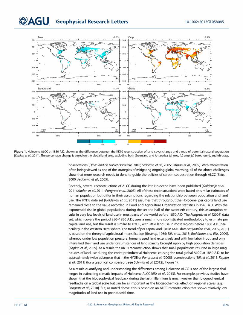
Figure 1. Holocene ALCC at 1850 A.D. shown as the difference between the KK10 reconstruction of land cover change and a map of potential natural vegetation[Kaplan et al., 2011]. The percentage change is based on the global land area, excluding both Greenland and Antarctica: (a) tree, (b) crop, (c) bareground, and (d) grass.

Geophysical Research Letters 10.1002/2013GL058085

HE ET AL. ©2013. American Geophysical Union. All Rights Reserved. 624

While regional studies have used KK10to investigate the biogeophysical im-pacts of ALCC on climate [Cook et al.,2012; Dermody et al., 2012], no study todate has used the KK10 reconstructionto examine the relative importanceof biogeophysical and biogeochemicalfeedbacks on global climate. In thisstudy we assess the relative impor-tance of biogeophysical and biogeo-chemical feedbacks to global climateby running the Community ClimateSystem Model, version 4 (CCSM4) [Gentet al., 2011] in a series of experiments,driven by different levels of greenhousegas concentrations, the KK10 ALCC sce-nario, and a control scenario with natu-

ral vegetation only. We further compare our results with previous model experiments that only consideredbiogeochemical feedbacks in Holocene climate change [Kutzbach et al., 2011; Ruddiman, 2003].

2. Model and Experiments

All simulations were performed at 1° resolution with the CCSM4 slab-ocean model, which is the atmosphere-sea ice-land mixed-layer ocean configuration of CCSM4 [Gent et al., 2011]. The 1° resolution is considerablyhigher than those in previous land use simulations, which are around 3–4° in Pitman et al. [2009], Davinand de Noblet-Ducoudre [2010], and Pongratz et al. [2010]. The atmosphere model is the CommunityAtmosphere Model, version 4, with a finite volume dynamical core and 26 layers in the vertical direction[Neale et al., 2013]. The sea ice model is the version 4 of the Los Alamos National Laboratory sea ice model(CICE4) [Holland et al., 2012]. The land model is the Community Land Model, version 4 (CLM4) [Lawrenceet al., 2012], with a carbon-nitrogen cycle model that is prognostic in carbon/nitrogen and vegetation phe-nology [Thornton et al., 2007]. CLM4 includes 14 natural plant functional types (PFTs) with eight tree PFTs, threeshrub PFTs, and three grass PFTs, plus one crop PFT and bareground [Lawrence and Chase, 2007; Oleson et al.,2010]. Compared with previous versions, CLM4 more realistically simulates snow cover, soil temperatures inorganic-rich soils, and extensive areas with near-surface permafrost [Lawrence et al., 2012]. The initial conditionsof all experiments were from the 1° CCSM4 slab-ocean control simulation for preindustrial period (~1850 A.D.).

We performed four experiments with CCSM4 to quantify biogeophysical and biogeochemical feedbacks(Table 1): two experiments to quantify the magnitude of ALCC-induced biogeophysical feedbacks and two toexamine the effects of changing greenhouse concentrations. The two experiments for biogeophysical effectsdiffered only in the distribution of PFTs that were input to CLM4, which had its dynamic vegetation optionturned off. The ALCC simulation used the KK10 land use map at 1850 A.D., and our control simulationused a reconstruction of potential natural vegetation [Kaplan et al., 2011]. In CLM4, two types of cropsare allowed to account for the different physiology of crops, but currently, only the first crop type isspecified in the surface data set [Oleson et al., 2010]. The KK10 fraction of used land was used to specifythe fractional coverage of the crop PFT; the fractional coverage of all of the other PFTs within a modelgrid cell was scaled accordingly to preserve their relative proportions. The maps of natural vegetationwere derived from Lund-Potsdam-Jena Dynamic Global Vegetation Model (LPJ DGVM) output [Sitch et al.,2003]. PFT cover fractions were then regrouped into PFT categories used by CCSM. The two experimentsfor biogeochemical effects differed only in the prescribed greenhouse gas concentrations (Table 2). Thegreenhouse gas values for Experiment PI (preindustrial period) were adopted from the National Centerfor Atmospheric Research (NCAR) CCSM4 preindustrial control simulation [Gent et al., 2011]. The green-house gas values for Experiment NA (no anthropogenic carbon emission) were adopted from Kutzbachet al. [2011], which are based on linear projection from earlier Holocene trends and coincide with theobserved values during stage 19, the closest analog to the Holocene among previous interglacials basedon the insolation variations [Tzedakis et al., 2012]. The experiments for biogeophysical and biogeochemical

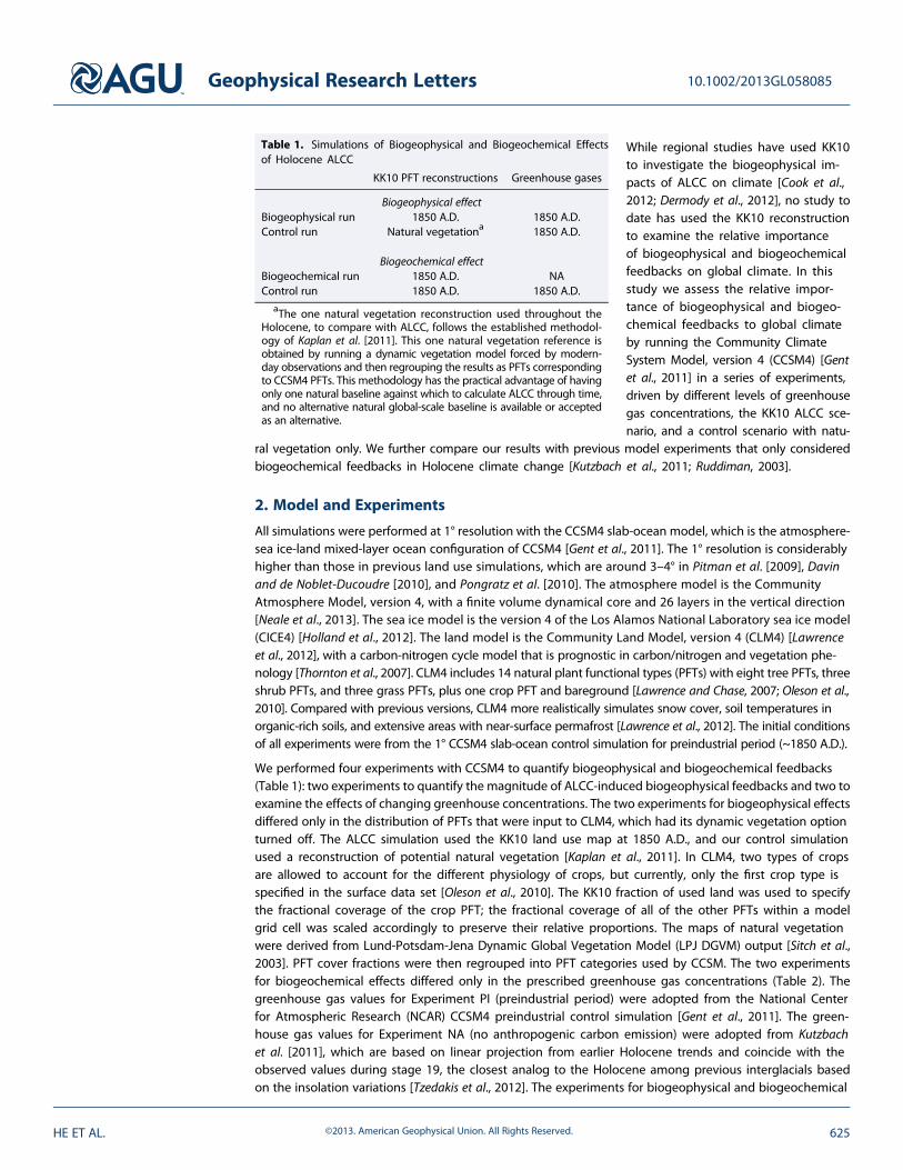
Table 1. Simulations of Biogeophysical and Biogeochemical Effectsof Holocene ALCC

KK10 PFT reconstructions Greenhouse gases

Biogeophysical effectBiogeophysical run 1850 A.D. 1850 A.D.Control run Natural vegetationa 1850 A.D.

Biogeochemical effectBiogeochemical run 1850 A.D. NAControl run 1850 A.D. 1850 A.D.

aThe one natural vegetation reconstruction used throughout theHolocene, to compare with ALCC, follows the established methodol-ogy of Kaplan et al. [2011]. This one natural vegetation reference isobtained by running a dynamic vegetation model forced by modern-day observations and then regrouping the results as PFTs correspondingto CCSM4 PFTs. This methodology has the practical advantage of havingonly one natural baseline against which to calculate ALCC through time,and no alternative natural global-scale baseline is available or acceptedas an alternative.

Geophysical Research Letters 10.1002/2013GL058085

HE ET AL. ©2013. American Geophysical Union. All Rights Reserved. 625

effects were run for 110 and 135 years, re-spectively, with the annual mean averagesof the last 50 years used for comparisons.

3. Results

In the KK10 scenario, land use at 1850 A.D.was concentrated in southeast NorthAmerica,parts of Central America, most of Europesouth of 60°N, the western portion of NorthAsia, southeast China, mainland SoutheastAsia, India, areas surrounding the tropicalrainforest in Africa, southern Africa, andnortheast Brazil (Figure 1b). In those regions,

25%–75% of natural vegetation had been converted into crops by 1850 A.D. The total amount of land underhuman use in 1850 A.D. was approximately 22 million km2, or 16.3% global land area. Of this total, 60% was landthat would naturally be forest and 33% would naturally be grassland (Figures 1a and 1d).

4. Biogeophysical Effects

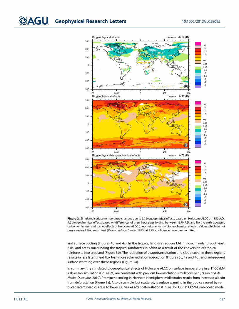
In the 1° CCSM4 slab-ocean simulation, the biogeophysical effect of Holocene ALCC causes broad cooling inthe midlatitudes of the Northern Hemisphere and scattered warming in mainland Southeast Asia, India, and inareas surrounding the tropical rainforest of Africa (Figure 2a). Overall, the global climate response to thebiogeophysical effect of Holocene ALCC is a cooling of 0.17°C, which is fivefold larger than the 0.03°C coolingcaused by the biogeophysical effect of ALCC during the last millennium estimated by Pongratz et al. [2010] inlow-resolution ECHAM5. As noted above, the Pongratz et al. [2010] scenario has relatively low amounts of landuse at 1850 A.D. compared to KK10, particularly in the Western Hemisphere.

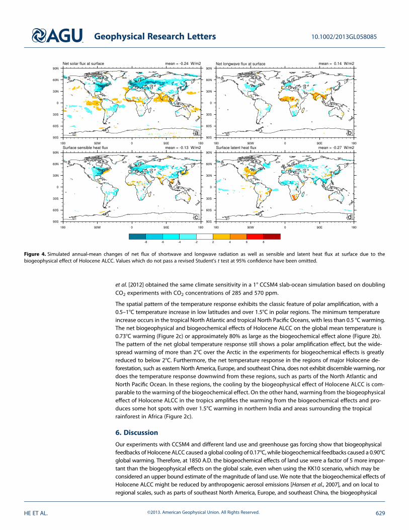
The broad cooling in the midlatitudes of the Northern Hemisphere is caused by increased albedo afterdeforestation. Since forests have lower surface albedo than cropland and can mask the high albedo ofunderlying snow, deforestation over North America, Europe, and China results in a widespread increaseof surface albedo of 0.01–0.05 across Northern Hemisphere midlatitudes (Figure 3a). As a result, the netsolar radiation flux at the surface is reduced by 2–8 W/m2 in these regions (Figure 4a), and this decreasecauses a widespread cooling of 0.25 to over 1°C in the midlatitude Northern Hemisphere (Figure 2a). Thelargest cooling (over 1°C) occurs locally where deforestation is greatest in North America and Europe(Figures 1a and 2a), but a significant cooling of over 0.5°C also occurs remotely over the North Atlanticand Asia, which are downwind of the largest ALCC over North America and Europe, respectively. The surfacecooling in the midlatitude Northern Hemisphere causes less loss of surface sensible heat (Figure 4c), whichpartly compensates the loss of the net surface solar radiation absorption caused by the increase of thesurface albedo.

Simulated albedo changes from Holocene ALCC are mostly confined to the midlatitudes of the NorthernHemisphere. For the land area of the tropics and Southern Hemisphere, surface temperature changes aremainly caused by the changes of the total leaf area index (LAI) resulting from Holocene ALCC (Figure 3b).The LAI changes can modify the surface latent heat fluxes through the changes of evapotranspiration(Figure 4d). For example, in the Southern Hemisphere, there is scattered cooling in northeast Brazil andsouthern Africa (Figure 2a). These regions are not associated with increased surface albedo but rather withan increase in the total leaf area index (LAI) (Figures 3a and 3b), which is mostly due to the conversion ofdeciduous forests and semiarid areas to croplands (Figure 1b). LAI increases also occur in the NorthernHemisphere, such as the southeast U.S., westernmost Europe, and southeastern China. In all of the abovefive regions, the LAI increase causes an increase of latent heat release due to increased evapotranspiration(Figure 4d), resulting in local cooling that is more discernible in the Southern Hemisphere. On the otherhand, increased evapotranspiration also causes increases in local clouds in all of these aforementionedregions except southeastern China (Figure 3c). More clouds reduce the net absorption of solar radiation atthe surface (Figure 4a). Surface heat flux loss from reduced solar radiation and enhanced latent heat flux isbalanced by the reduction of heat flux loss from net longwave and sensible heat due to increases in clouds

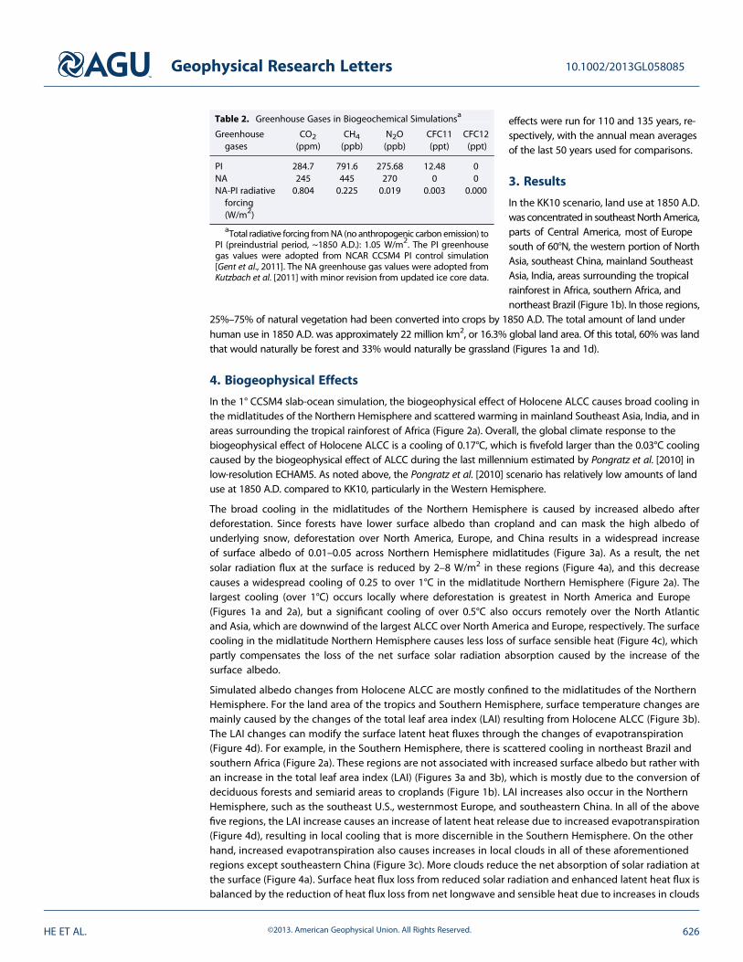
Table 2. Greenhouse Gases in Biogeochemical Simulationsa

Greenhousegases

CO2(ppm)

CH4(ppb)

N2O(ppb)

CFC11(ppt)

CFC12(ppt)

PI 284.7 791.6 275.68 12.48 0NA 245 445 270 0 0NA-PI radiativeforcing(W/m2)

0.804 0.225 0.019 0.003 0.000

aTotal radiative forcing fromNA (no anthropogenic carbon emission) toPI (preindustrial period, ~1850 A.D.): 1.05 W/m2. The PI greenhousegas values were adopted from NCAR CCSM4 PI control simulation[Gent et al., 2011]. The NA greenhouse gas values were adopted fromKutzbach et al. [2011] with minor revision from updated ice core data.

Geophysical Research Letters 10.1002/2013GL058085

HE ET AL. ©2013. American Geophysical Union. All Rights Reserved. 626

and surface cooling (Figures 4b and 4c). In the tropics, land use reduces LAI in India, mainland SoutheastAsia, and areas surrounding the tropical rainforests in Africa as a result of the conversion of tropicalrainforests into cropland (Figure 3b). The reduction of evapotranspiration and cloud cover in these regionsresults in less latent heat flux loss, more solar radiation absorption (Figures 3c, 4a and 4d), and subsequentsurface warming over these regions (Figure 2a).

In summary, the simulated biogeophysical effects of Holocene ALCC on surface temperature in a 1° CCSM4slab-ocean simulation (Figure 2a) are consistent with previous low-resolution simulations [e.g., Davin and deNoblet-Ducoudre, 2010]. Prominent cooling in Northern Hemisphere midlatitudes results from increased albedofrom deforestation (Figure 3a). Also discernible, but scattered, is surface warming in the tropics caused by re-duced latent heat loss due to lower LAI values after deforestation (Figure 3b). Our 1° CCSM4 slab-ocean model

Figure 2. Simulated surface temperature changes due to (a) biogeophysical effects based on Holocene ALCC at 1850 A.D.,(b) biogeochemical effects based on differences of greenhouse gas forcing between 1850 A.D. and NA (no anthropogeniccarbon emission), and (c) net effects of Holocene ALCC (biophysical effects + biogeochemical effects). Values which do notpass a revised Student’s t test [Zwiers and von Storch, 1995] at 95% confidence have been omitted.

Geophysical Research Letters 10.1002/2013GL058085

HE ET AL. ©2013. American Geophysical Union. All Rights Reserved. 627

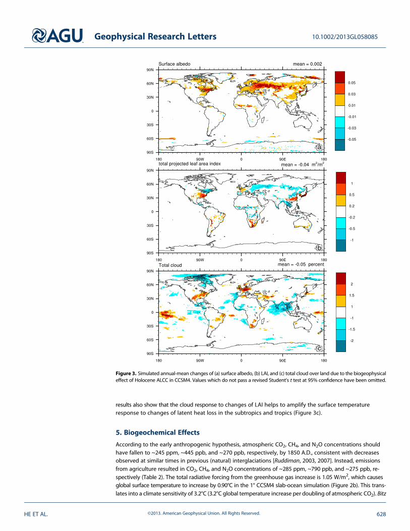
results also show that the cloud response to changes of LAI helps to amplify the surface temperatureresponse to changes of latent heat loss in the subtropics and tropics (Figure 3c).

5. Biogeochemical Effects

According to the early anthropogenic hypothesis, atmospheric CO2, CH4, and N2O concentrations shouldhave fallen to ~245 ppm, ~445 ppb, and ~270 ppb, respectively, by 1850 A.D., consistent with decreasesobserved at similar times in previous (natural) interglaciations [Ruddiman, 2003, 2007]. Instead, emissionsfrom agriculture resulted in CO2, CH4, and N2O concentrations of ~285 ppm, ~790 ppb, and ~275 ppb, re-spectively (Table 2). The total radiative forcing from the greenhouse gas increase is 1.05 W/m2, which causesglobal surface temperature to increase by 0.90°C in the 1° CCSM4 slab-ocean simulation (Figure 2b). This trans-lates into a climate sensitivity of 3.2°C (3.2°C global temperature increase per doubling of atmospheric CO2). Bitz

Figure 3. Simulated annual-mean changes of (a) surface albedo, (b) LAI, and (c) total cloud over land due to the biogeophysicaleffect of Holocene ALCC in CCSM4. Values which do not pass a revised Student’s t test at 95% confidence have been omitted.

Geophysical Research Letters 10.1002/2013GL058085

HE ET AL. ©2013. American Geophysical Union. All Rights Reserved. 628

et al. [2012] obtained the same climate sensitivity in a 1° CCSM4 slab-ocean simulation based on doublingCO2 experiments with CO2 concentrations of 285 and 570 ppm.

The spatial pattern of the temperature response exhibits the classic feature of polar amplification, with a0.5–1°C temperature increase in low latitudes and over 1.5°C in polar regions. The minimum temperatureincrease occurs in the tropical North Atlantic and tropical North Pacific Oceans, with less than 0.5 °C warming.The net biogeophysical and biogeochemical effects of Holocene ALCC on the global mean temperature is0.73°C warming (Figure 2c) or approximately 80% as large as the biogeochemical effect alone (Figure 2b).The pattern of the net global temperature response still shows a polar amplification effect, but the wide-spread warming of more than 2°C over the Arctic in the experiments for biogeochemical effects is greatlyreduced to below 2°C. Furthermore, the net temperature response in the regions of major Holocene de-forestation, such as eastern North America, Europe, and southeast China, does not exhibit discernible warming, nordoes the temperature response downwind from these regions, such as parts of the North Atlantic andNorth Pacific Ocean. In these regions, the cooling by the biogeophysical effect of Holocene ALCC is com-parable to the warming of the biogeochemical effect. On the other hand, warming from the biogeophysicaleffect of Holocene ALCC in the tropics amplifies the warming from the biogeochemical effects and pro-duces some hot spots with over 1.5°C warming in northern India and areas surrounding the tropicalrainforest in Africa (Figure 2c).

6. Discussion

Our experiments with CCSM4 and different land use and greenhouse gas forcing show that biogeophysicalfeedbacks of Holocene ALCC caused a global cooling of 0.17°C, while biogeochemical feedbacks caused a 0.90°Cglobal warming. Therefore, at 1850 A.D. the biogeochemical effects of land use were a factor of 5 more impor-tant than the biogeophysical effects on the global scale, even when using the KK10 scenario, which may beconsidered an upper bound estimate of the magnitude of land use. We note that the biogeochemical effects ofHolocene ALCC might be reduced by anthropogenic aerosol emissions [Hansen et al., 2007], and on local toregional scales, such as parts of southeast North America, Europe, and southeast China, the biogeophysical

Figure 4. Simulated annual-mean changes of net flux of shortwave and longwave radiation as well as sensible and latent heat flux at surface due to thebiogeophysical effect of Holocene ALCC. Values which do not pass a revised Student’s t test at 95% confidence have been omitted.

Geophysical Research Letters 10.1002/2013GL058085

HE ET AL. ©2013. American Geophysical Union. All Rights Reserved. 629

effects of Holocene ALCC induce prominent cooling due to albedo increases from deforestation and are able toreduce or cancel regional warming caused by biogeochemical feedbacks. We also note that this study does notaddress the timing of global and regional effects of Holocene ALCC, which will be addressed in ourupcoming research.

The net effect of Holocene ALCC amounts to a global warming of 0.73°C during the preindustrial era in oursimulations (Figure 2c) and is comparable to the ~0.8°C warming during industrial time [Hansen et al., 2010].The lack of ocean dynamics in the 1° CCSM4 slab-ocean simulations could underestimate the climate sensi-tivity because of the lack of feedbacks from ocean heat transport [Kutzbach et al., 2013; Manabe and Bryan,1985]. In 1° CCSM4 fully coupled simulations, the climate sensitivity is ~65% larger than the 1° CCSM4 slab-ocean simulations during the Holocene (5.3°C versus 3.2°C) [Kutzbach et al., 2013]. With this greater climatesensitivity, we could speculate that the biogeochemical effects of Holocene ALCC could have caused a globalwarming of ~1.5°C, and the net biogeophysical and biogeochemical effects of Holocene ALCC could cause aglobal warming of 1.2 °C during the preindustrial era in our simulations, which is 50% higher than the globalwarming of ~0.8°C during industrial times. Therefore, the net effects of Holocene ALCC support the centraltheme of the early anthropogenic hypothesis that the human impact on global climate started thousands ofyears before the Industrial Revolution as a result of the greenhouse gas emissions caused by farming activ-ities such as deforestation and rice cultivation [Ruddiman, 2003, 2007, 2013].

ReferencesBala, G., K. Caldeira, M. Wickett, T. J. Phillips, D. B. Lobell, C. Delire, and A. Mirin (2007), Combined climate and carbon-cycle effects of large-

scale deforestation, Proc. Natl. Acad. Sci. U. S. A., 104(16), 6550–6555.Betts, R. A. (2000), Offset of the potential carbon sink from boreal forestation by decreases in surface albedo, Nature, 408(6809), 187–190.Bitz, C. M., K. M. Shell, P. R. Gent, D. A. Bailey, G. Danabasoglu, K. C. Armour, M. M. Holland, and J. T. Kiehl (2012), Climate Sensitivity of the

Community Climate System Model, Version 4, J. Clim., 25(9), 3053–3070.Boserup, E. (1965), The Conditions of Agricultural Growth: The Economics of Agrarian Change Under Population Pressure, Aldine Pub. Co., Chicago.Brovkin, V., S. Sitch, W. von Bloh, M. Claussen, E. Bauer, and W. Cramer (2004), Role of land cover changes for atmospheric CO2 increase and

climate change during the last 150 years, Global Change Biol., 10(8), 1253–1266.Claussen, M., V. Brovkin, and A. Ganopolski (2001), Biogeophysical versus biogeochemical feedbacks of large-scale land cover change,

Geophys. Res. Lett., 28(6), 1011–1014.Cook, B. I., K. J. Anchukaitis, J. O. Kaplan, M. J. Puma, M. Kelley, and D. Gueyffier (2012), Pre-Columbian deforestation as an amplifier of

drought in Mesoamerica, Geophys. Res. Lett., 39, L16706, doi:10.1029/2012GL052565.Davin, E. L., and N. de Noblet-Ducoudre (2010), Climatic impact of global-scale deforestation: Radiative versus nonradiative processes,

J. Clim., 23(1), 97–112.Dermody, B. J., H. J. de Boer, M. F. P. Bierkens, S. L. Weber, M. J. Wassen, and S. C. Dekker (2012), A seesaw in Mediterranean precipitation

during the Roman period linked to millennial-scale changes in the North Atlantic, Clim. Past, 8(2), 637–651.Ellis, E. C., K. K. Goldewijk, S. Siebert, D. Lightman, and N. Ramankutty (2010), Anthropogenic transformation of the biomes, 1700 to 2000,

Global Ecol. Biogeogr., 19(5), 589–606.Ellis, E. C., J. O. Kaplan, D. Q. Fuller, S. Vavrus, K. Klein Goldewijk, and P. H. Verburg (2013), Used planet: A global history, Proc. Natl. Acad. Sci. U S A,

110(20), 7978–7985.Feddema, J. J., K. W. Oleson, G. B. Bonan, L. O. Mearns, L. E. Buja, G. A. Meehl, and W. M. Washington (2005), The importance of land-cover change in

simulating future climates, Science, 310(5754), 1674–1678.Gent, P. R., et al. (2011), The Community Climate System Model Version 4, J. Clim., 24(19), 4973–4991.Goldewijk, K. K. (2001), Estimating global land use change over the past 300 years: The HYDE database, Global Biogeochem. Cycles, 15(2),

417–433.Goldewijk, K. K., A. Beusen, G. van Drecht, and M. de Vos (2011), The HYDE 3.1 spatially explicit database of human-induced global land-use

change over the past 12,000 years, Global Ecol. Biogeogr., 20(1), 73–86.Hansen, J., M. Sato, P. Kharecha, G. Russell, D. W. Lea, and M. Siddall (2007), Climate change and trace gases, Philos. Trans. Ser. A Math. Phys.

Eng. Sci., 365(1856), 1925–1954.Hansen, J., R. Ruedy, M. Sato, and K. Lo (2010), Global surface temperature change, Rev. Geophys., 48, RG4004, doi:10.1029/2010RG000345.Holland, M. M., D. A. Bailey, B. P. Briegleb, B. Light, and E. Hunke (2012), Improved sea ice shortwave radiation physics in CCSM4: The impact

of melt ponds and aerosols on Arctic sea ice, J. Clim., 25(5), 1413–1430.Kaplan, J. O., K. M. Krumhardt, and N. Zimmermann (2009), The prehistoric and preindustrial deforestation of Europe, Quat. Sci. Rev., 28(27-28),

3016–3034.Kaplan, J. O., K. M. Krumhardt, E. C. Ellis, W. F. Ruddiman, C. Lemmen, and K. K. Goldewijk (2011), Holocene carbon emissions as a result of

anthropogenic land cover change, Holocene, 21(5), 775–791.Kutzbach, J. E., S. J. Vavrus, W. F. Ruddiman, and G. Philippon-Berthier (2011), Comparisons of atmosphere-ocean simulations of green-

house gas-induced climate change for pre-industrial and hypothetical ‘no-anthropogenic’ radiative forcing, relative to presentday, Holocene, 21(5), 793–801.

Kutzbach, J. E., F. He, S. J. Vavrus, and W. F. Ruddiman (2013), The dependence of equilibrium climate sensitivity on climate state: Applications tostudies of climates colder than present, Geophys. Res. Lett., 40, 3721–3726, doi:10.1002/grl.50724.

Lawrence, D. M., K. W. Oleson, M. G. Flanner, C. G. Fletcher, P. J. Lawrence, S. Levis, S. C. Swenson, and G. B. Bonan (2012), The CCSM4 landsimulation, 1850–2005: Assessment of surface climate and new capabilities, J. Clim., 25(7), 2240–2260.

Lawrence, P. J., and T. N. Chase (2007), Representing a new MODIS consistent land surface in the Community Land Model (CLM 3.0),J. Geophys. Res., 112, G01023, doi:10.1029/2006JG000168.

AcknowledgmentsThis work was supported by NationalScience Foundation grants ATM-0602270,ATM-0902802, and AGS-1203430 to theUniversity of Wisconsin-Madison and ATM-0902982 and AGS-1203965 to theUniversity of Virginia. Computational sup-port was provided by NCAR’s ClimateSimulation Laboratory, which is supportedby the National Science Foundation. Weappreciate the discussions with Erle Ellis.This is CCR contribution no. 1167.

The Editor thanks two anonymous re-viewers for their assistance in evaluating thispaper.

Geophysical Research Letters 10.1002/2013GL058085

HE ET AL. ©2013. American Geophysical Union. All Rights Reserved. 630

Manabe, S., and K. Bryan (1985), CO2-induced change in a coupled ocean-atmosphere model and its paleoclimatic implications, J. Geophys.Res., 90(Nc6), 1689–1707.

Matthews, H. D., A. J. Weaver, K. J. Meissner, N. P. Gillett, and M. Eby (2004), Natural and anthropogenic climate change: Incorporating his-torical land cover change, vegetation dynamics and the global carbon cycle, Clim. Dyn., 22(5), 461–479.

Neale, R. B., J. Richter, S. Park, P. H. Lauritzen, S. J. Vavrus, P. J. Rasch, and M. Zhang (2013), The Mean Climate of the Community AtmosphereModel (CAM4) in forced SST and fully coupled experiments, J. Clim., 26(14), 5150–5168.

Oleson, K. W., D. M. Lawrence, G. B. Bonan, M. G. Flanner, E. Kluzek, P. J. Lawrence, S. Levis, S. C. Swenson, and P. E. Thornton (2010), Technicaldescription of version 4.0 of the Community Land Model (CLM), NCAR Technical Note.

Pitman, A. J., et al. (2009), Uncertainties in climate responses to past land cover change: First results from the LUCID intercomparison study,Geophys. Res. Lett., 36, L14814, doi:10.1029/2009GL039076.

Pitman, A.J., A. Arneth, L. Ganzeveld, 2012, Regionalizing global climate models, Int. J. Climatol., 32, 321–337, doi:10.1002/joc.2279.Pongratz, J., C. Reick, T. Raddatz, and M. Claussen (2008), A reconstruction of global agricultural areas and land cover for the last millennium,

Global Biogeochem. Cycles, 22, GB3018, doi:10.1029/2007GB003153.Pongratz, J., C. H. Reick, T. Raddatz, and M. Claussen (2010), Biogeophysical versus biogeochemical climate response to historical

anthropogenic land cover change, Geophys. Res. Lett., 37, L08702, doi:10.1029/2010GL043010.Ramankutty, N., and J. A. Foley (1999), Estimating historical changes in global land cover: Croplands from 1700 to 1992, Global Biogeochem.

Cycles, 13(4), 997–1027.Ruddiman, W. F. (2003), The anthropogenic greenhouse era began thousands of years ago, Clim. Change, 61(3), 261–293.Ruddiman, W. F. (2007), The early anthropogenic hypothesis: Challenges and responses, Rev. Geophys., 45, RG4001, doi:10.1029/

2006RG000207.Ruddiman, W. F. (2013), The Anthropocene, Annu. Rev. Earth Planet. Sci., 41(1), 45–68.Ruddiman, W. F., and E. C. Ellis (2009), Effect of per-capita land use changes on Holocene forest clearance and CO2 emissions, Quat. Sci. Rev.,

28(27-28), 3011–3015.Schmidt, G. A., et al. (2012), Climate forcing reconstructions for use in PMIP simulations of the Last Millennium (v1.1), Geosci. Model Dev., 5(1),

185–191.Sitch, S., et al. (2003), Evaluation of ecosystem dynamics, plant geography and terrestrial carbon cycling in the LPJ dynamic global vegetation

model, Global Change Biol., 9(2), 161–185.Stocker, T. F., D. Qin, G. K. Plattner, M. Tignor, S. K. Allen, J. Boschung, A. Nauels, Y. Xia, V. Bex, and P. M. Midgley (Eds.) (2013), IPCC, 2013:

Summary for policymakers, in Climate Change 2013: The Physical Science Basis. Contribution of Working Group I to the Fifth Assessment Report of theIntergovernmental Panel on Climate Change, pp. 1–27, Cambridge Univ. Press, Cambridge, U.K., and New York.

Thornton, P. E., J. F. Lamarque, N. A. Rosenbloom, and N. M. Mahowald (2007), Influence of carbon-nitrogen cycle coupling on land model re-sponse to CO2 fertilization and climate variability, Global Biogeochem. Cycles, 21, GB4018, doi:10.1029/2006GB002868.

Tzedakis, P. C., J. E. T. Channell, D. A. Hodell, H. F. Kleiven, and L. C. Skinner (2012), Determining the natural length of the current interglacial,Nat. Geosci., 5(2), 138–141.

Zwiers, F. W., and H. von Storch (1995), Taking serial correlation into account in tests of the mean, J. Clim., 8(2), 336–351.

Geophysical Research Letters 10.1002/2013GL058085

HE ET AL. ©2013. American Geophysical Union. All Rights Reserved. 631