Embed Size (px)
Citation preview

Simulating fabrication of an all‐Silicon pressure sensor
Overview
• All‐silicon pressure sensor– Why silicon?– Operating principle
• The fabrication process– Step‐by‐step description
• The simulation challenge– Duplication of the fabrication process– Meshing, loads and boundary conditions
• Results
Silicon in the electronics industry
• Why silicon?– Abundance– Precise, well understood processing methods well suited for
miniaturization– Processing is based on photographic techniques well suited
for miniaturization– Batch fabrication producing hundreds of identical devices
on one single wafer• Uses driven by silicon’s mechanical properties
– Sensor & transducers• Micromechanical and nano‐scale devices created using chemical etching and thin film deposits
– Easy integration of devices with integrated circuits
All‐Silicon pressure transducers
• Operating principle– The diaphragm is made of a thin layer of silicon– A Wheatstone bridge circuit is created on top of the diaphragm
– Deflection of the diaphragm due to applied pressure is detected as a resistance change which is easily correlated to the applied pressure
– This type of sensor can be made to measure gauge or absolute pressure
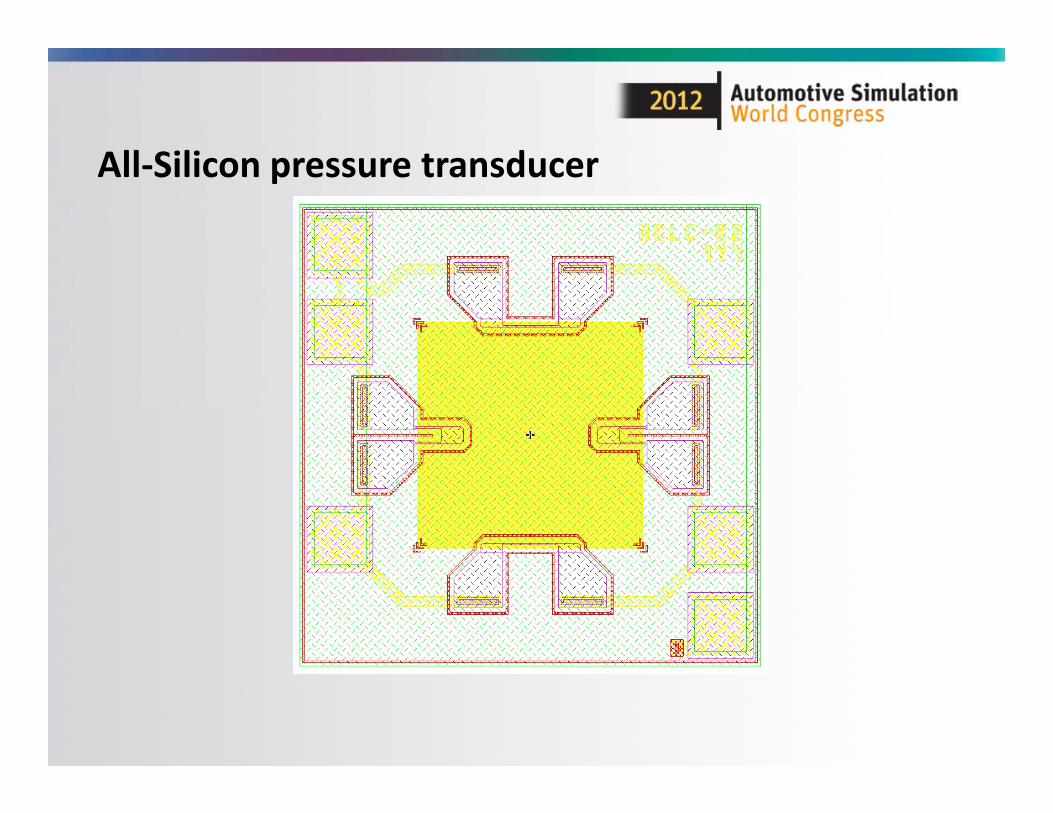
All‐Silicon pressure transducer

The Fabrication Process
• The fabrication process is modeled as follows:– Step 1: The Si substrate, a 1 u thick layer of Sio2, and a
768u Si layer is cooled from 1050C (stress free temperature) to room temperature
– Step 2: Excess silicon is removed using a grinding process to produce a 15u‐thick diaphragm
– Step 3: Diaphragm is formed by etching a cavity in the substrate at room temperature
– Step 4: Increase the assembly temperature to 450C– Step 5: Attach the glass pedestal– Step 6: Cool down to room temperature
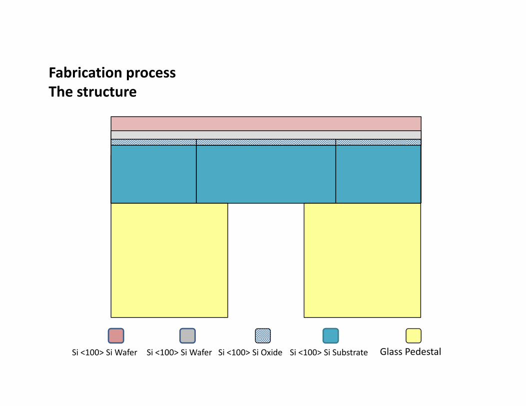
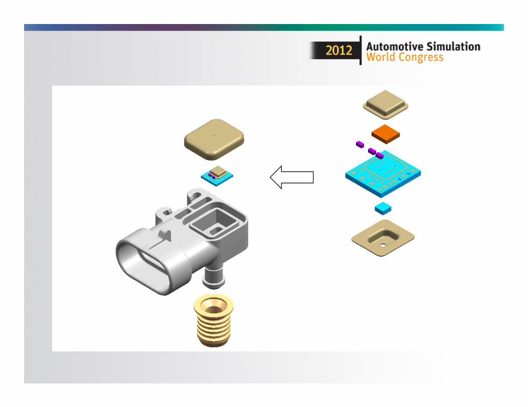
Fabrication processThe structure
Si <100> Si Wafer Si <100> Si Wafer Si <100> Si Oxide Si <100> Si Substrate Glass Pedestal
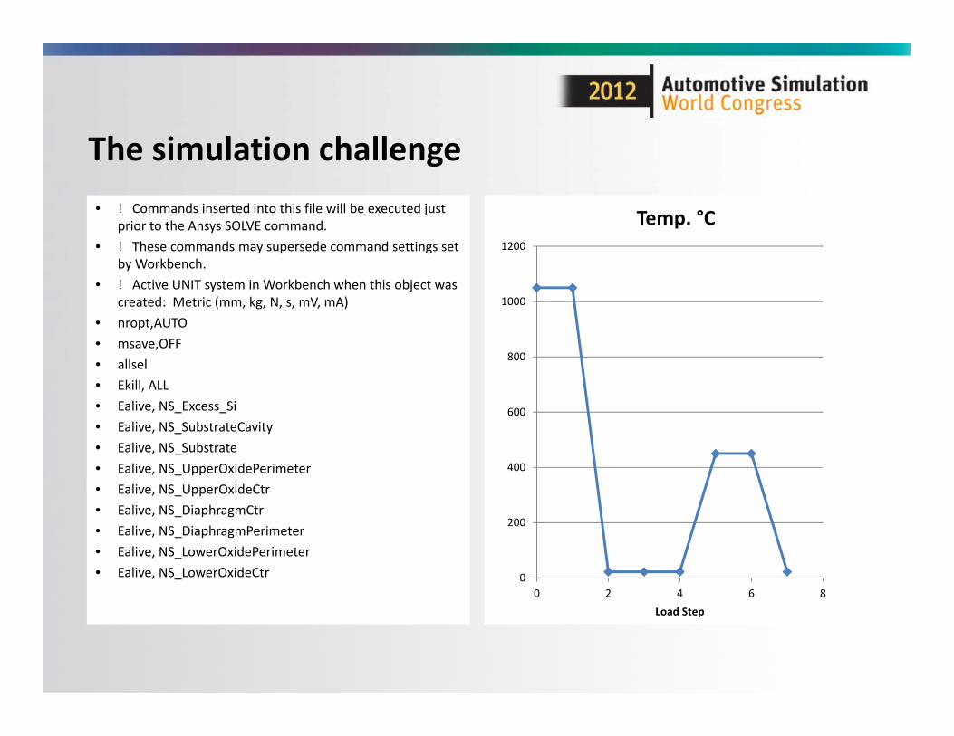
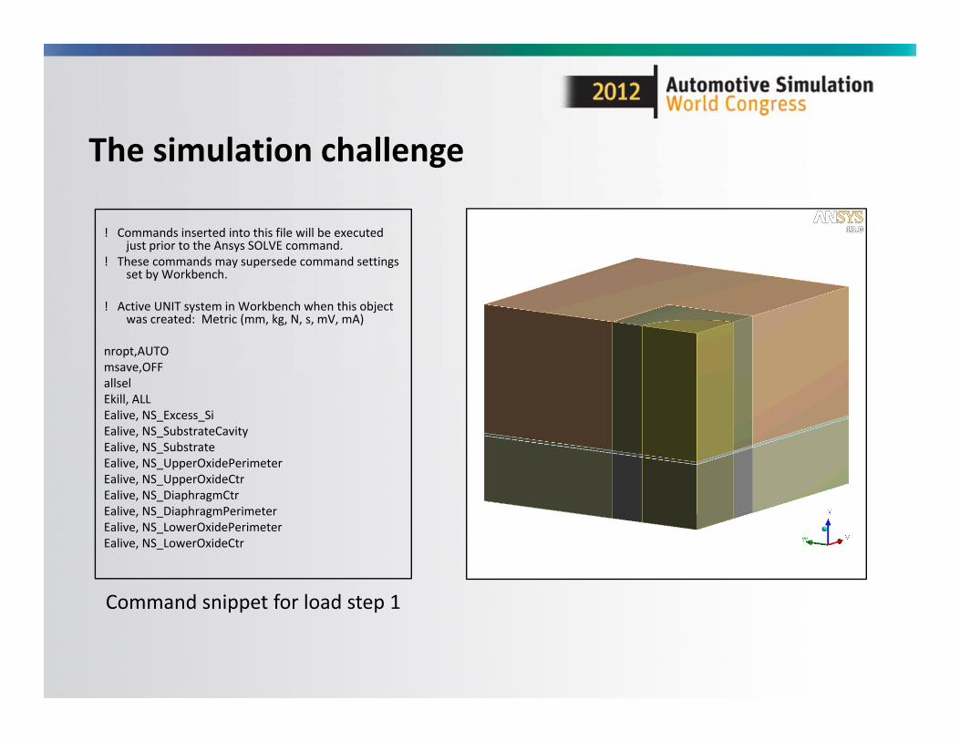
The simulation challenge• ! Commands inserted into this file will be executed just
prior to the Ansys SOLVE command.• ! These commands may supersede command settings set
by Workbench.• ! Active UNIT system in Workbench when this object was
created: Metric (mm, kg, N, s, mV, mA)• nropt,AUTO• msave,OFF• allsel• Ekill, ALL• Ealive, NS_Excess_Si• Ealive, NS_SubstrateCavity• Ealive, NS_Substrate• Ealive, NS_UpperOxidePerimeter• Ealive, NS_UpperOxideCtr• Ealive, NS_DiaphragmCtr• Ealive, NS_DiaphragmPerimeter• Ealive, NS_LowerOxidePerimeter• Ealive, NS_LowerOxideCtr 0
200
400
600
800
1000
1200
0 2 4 6 8Load Step
Temp. °C
The simulation challenge
• Goals of the analysis– Simulate the fabrication process to determine if significant residual stresses exist in the final structure
• Pressure sensor model– Create a model that can be subjected to additional manufacturing and/or operating loads
– Determine if the existence of a 1 µ oxide layer contributes to the failure of the diaphragm
The simulation challenge
• Material addition and removal at different temperatures– Single crystal silicon, silicon oxide and pedestal material are added and
removed by different means and at different temperatures– Normally the simulation would start with the final structure and model
the heating and or cooling of the entire structure– This procedure ignores the strains that may have been locked into the
remaining structure – For best results, the simulation process should follow the fabrication
process as closely as possible• Final sensor model
– The final sensor model is carved out of the original model as a substructure and can be subjected to additional loads• In the initial mode, the pressure surfaces of the diaphragm are covered and can
not be directly accessed for loading• Even without the above requirement, the extreme thickness difference of adjacent
layers of the model may make substructuring necessary
The simulation challenge
• Finite Element Modeling of the fabrication process– The sensor structure is symmetric, therefore a quarter‐symmetry model
is used– In order to model the fabrication steps, the complete structure including
the glass pedestal, excess substrate material and excess material on top of the diaphragm must be modeled from the beginning of the analysis
– At each step of the process, the appropriate elements representing the sensor structures are “killed” or brought to life to simulate the process at that step
– This presentation describes the process of using ANSYS Mechanical in combination with DesignModeler and Mechanical APDL commands (command snippets)
– DesignModeler (or another commercial CAD package) allows the creation of the solid model of the final structure relatively easily• Creation of an extruded mesh of the structure (most efficient) requires some
additional work
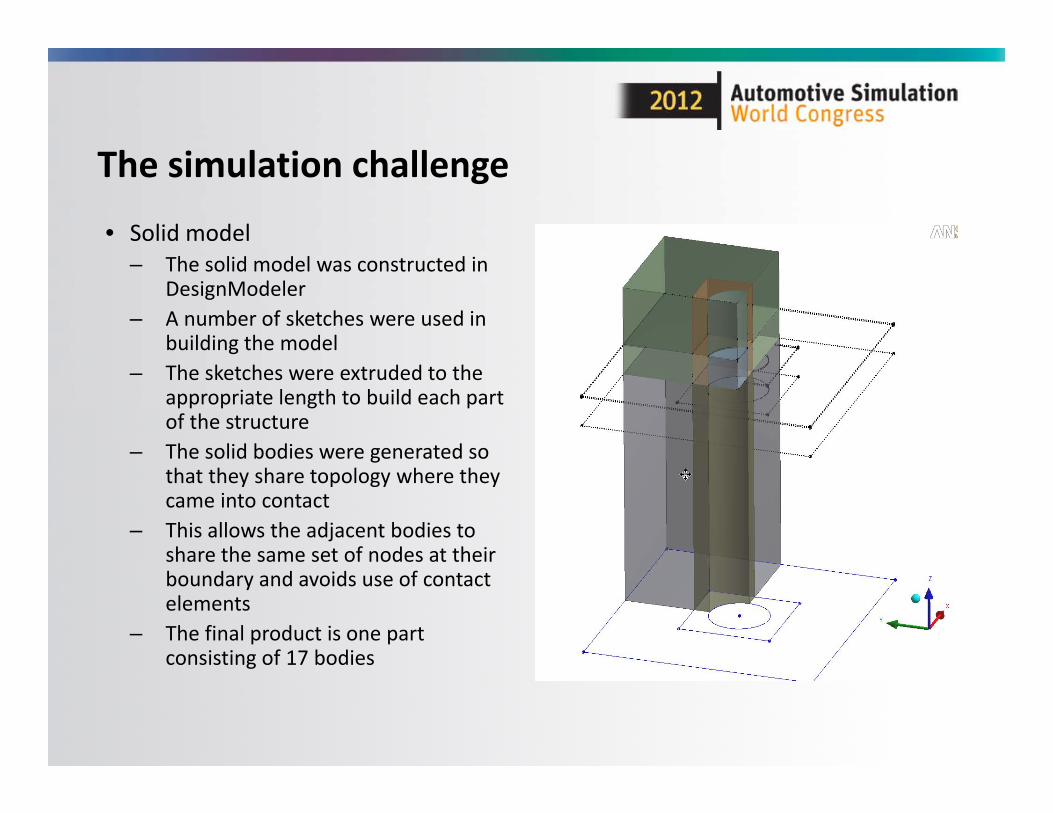
The simulation challenge
• Solid model– The solid model was constructed in
DesignModeler– A number of sketches were used in
building the model– The sketches were extruded to the
appropriate length to build each part of the structure
– The solid bodies were generated so that they share topology where they came into contact
– This allows the adjacent bodies to share the same set of nodes at their boundary and avoids use of contact elements
– The final product is one part consisting of 17 bodies
The simulation challenge
• Use of named selections– Prior to generating the mesh the solid model was divided into a number
of groupings based on their role in the creation of the sensor– During the solution phase, the named selections easily identify the
elements that have to be added or removed using the ANSYS “EALIVE” or EKILL commands
• FE mesh– The geometry of the sensor device is such that it lends itself easily to
being meshed by sweeping– The Mechanical “Sweep Method” allows specification of the number of
divisions as well as biasing – The sensor structure consists of very thin layers attached to relatively
thick layers of material which can lead to generation of very large meshes
– Biasing helps reduce the size of the model without sacrificing accuracy
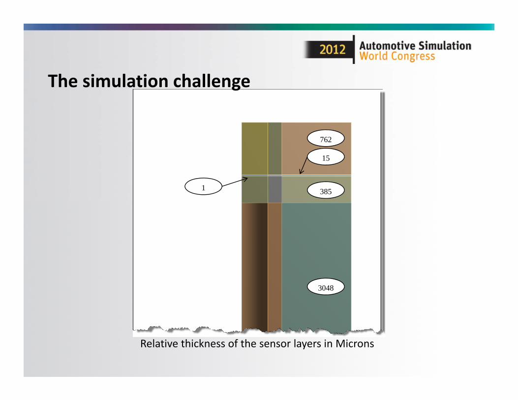
The simulation challenge
762
15
1 385
3048
Relative thickness of the sensor layers in Microns
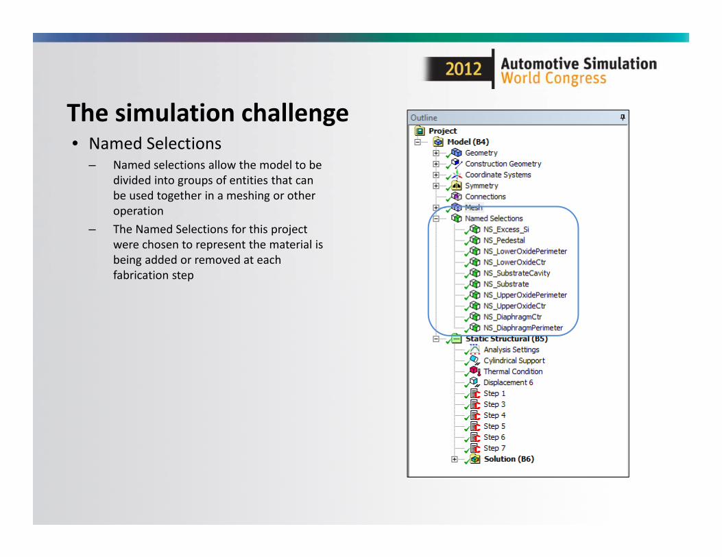
The simulation challenge• Named Selections
– Named selections allow the model to be divided into groups of entities that can be used together in a meshing or other operation
– The Named Selections for this project were chosen to represent the material is being added or removed at each fabrication step

The simulation challenge• Mesh Controls
– The desired mesh can be obtained by using the Sweep method along with element size specification
– The element size and number of divisions can be arrived at by considering the thickness of the layers as well as their role in the complete structure
– The bias feature of the Sweep Method allows fine‐tuning of the mesh by ensuring that sufficient number of elements are created at the critical areas of the structure
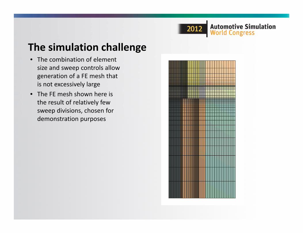
The simulation challenge• The combination of element
size and sweep controls allow generation of a FE mesh that is not excessively large
• The FE mesh shown here is the result of relatively few sweep divisions, chosen for demonstration purposes

The simulation challenge
– Use of command snippets• This feature of Workbench/Mechanical allows inclusion of APDL commands in various stages of the analysis (Prep7/Solution/Post1/Post26)
• This feature takes advantages of the strengths of both Mechanical and Mechanical APDL
• The sub‐structuring process was implemented in Mechanical APDL– Once a model is set up and ready for execution, ANSYS Mechanical
writes an ASCII file for the solver to read and execute– The user can instruct Mechanical to write this file without executing it– The file can then be edited or the user can use Mechanical APDL
interactively to complete the analysis
The simulation challenge
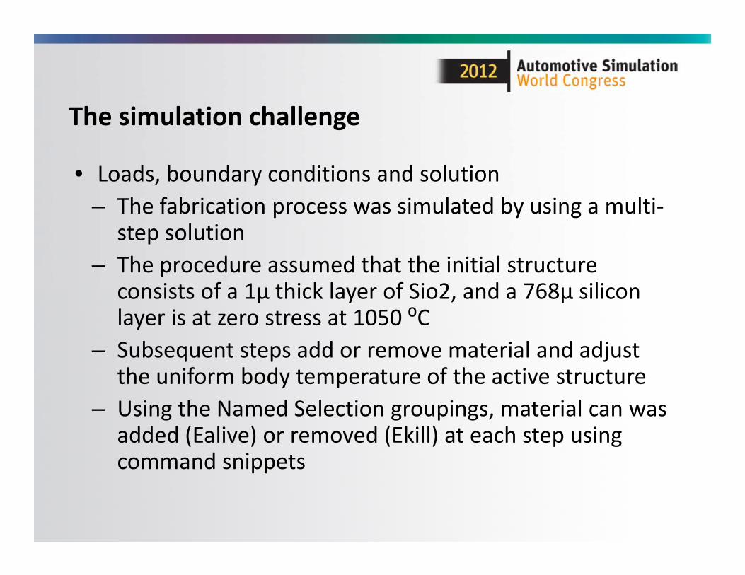
• Loads, boundary conditions and solution– The fabrication process was simulated by using a multi‐
step solution– The procedure assumed that the initial structure
consists of a 1µ thick layer of Sio2, and a 768µ silicon layer is at zero stress at 1050 ⁰C
– Subsequent steps add or remove material and adjust the uniform body temperature of the active structure
– Using the Named Selection groupings, material can was added (Ealive) or removed (Ekill) at each step using command snippets
The simulation challenge
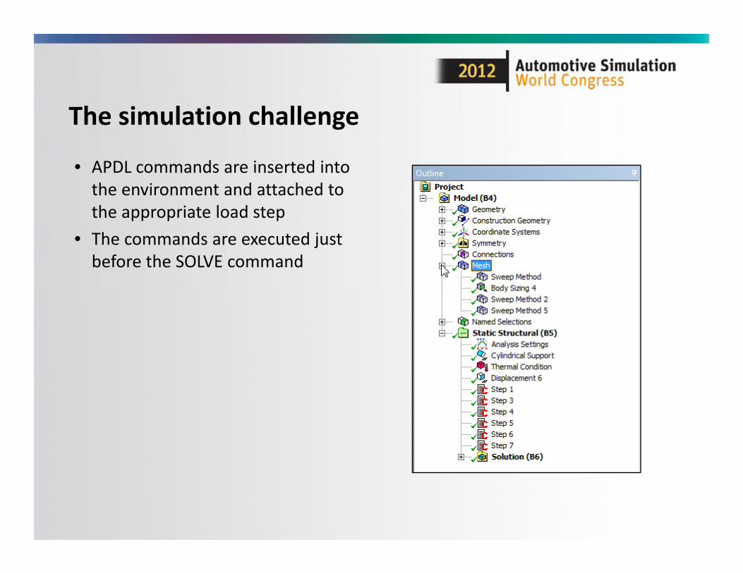
• APDL commands are inserted into the environment and attached to the appropriate load step
• The commands are executed just before the SOLVE command
The simulation challenge
! Commands inserted into this file will be executed just prior to the Ansys SOLVE command.
! These commands may supersede command settings set by Workbench.
! Active UNIT system in Workbench when this object was created: Metric (mm, kg, N, s, mV, mA)
nropt,AUTOmsave,OFFallselEkill, ALLEalive, NS_Excess_SiEalive, NS_SubstrateCavityEalive, NS_SubstrateEalive, NS_UpperOxidePerimeterEalive, NS_UpperOxideCtrEalive, NS_DiaphragmCtrEalive, NS_DiaphragmPerimeterEalive, NS_LowerOxidePerimeterEalive, NS_LowerOxideCtr
Command snippet for load step 1

The simulation challenge
!Kill the excess SiEkill,NS_Excess_Si
Command snippet for load step 3
The simulation challenge
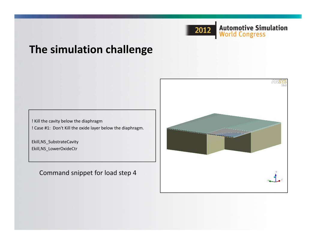
! Kill the cavity below the diaphragm! Case #1: Don't Kill the oxide layer below the diaphragm.
Ekill,NS_SubstrateCavityEkill,NS_LowerOxideCtr
Command snippet for load step 4
The simulation challenge
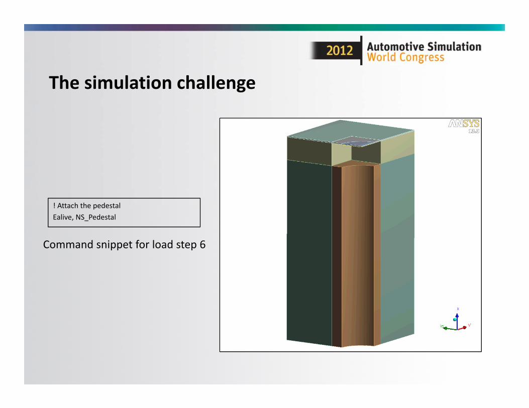
! Attach the pedestalEalive, NS_Pedestal
Command snippet for load step 6

The simulation challenge
• Substructuring– The simulation steps described thus far constitute the creation and analysis of the coarse model in a substructuring operation
– Once this process was completed a submodel was created by changing the meshing controls of the original model to create a refined mesh
– The remaining steps (cut boundary interrpolationand analysis of the submodel) were performed in mechanical APDL using a number of APDL macros
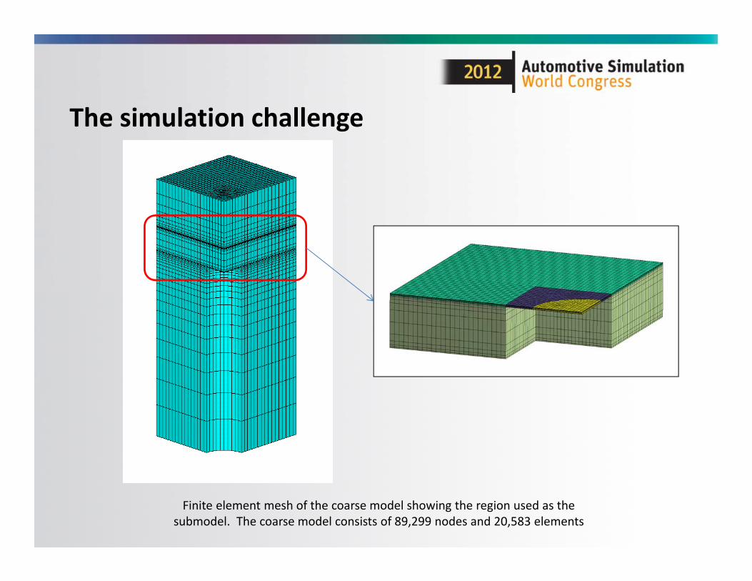
The simulation challenge
Finite element mesh of the coarse model showing the region used as the submodel. The coarse model consists of 89,299 nodes and 20,583 elements
The simulation challenge
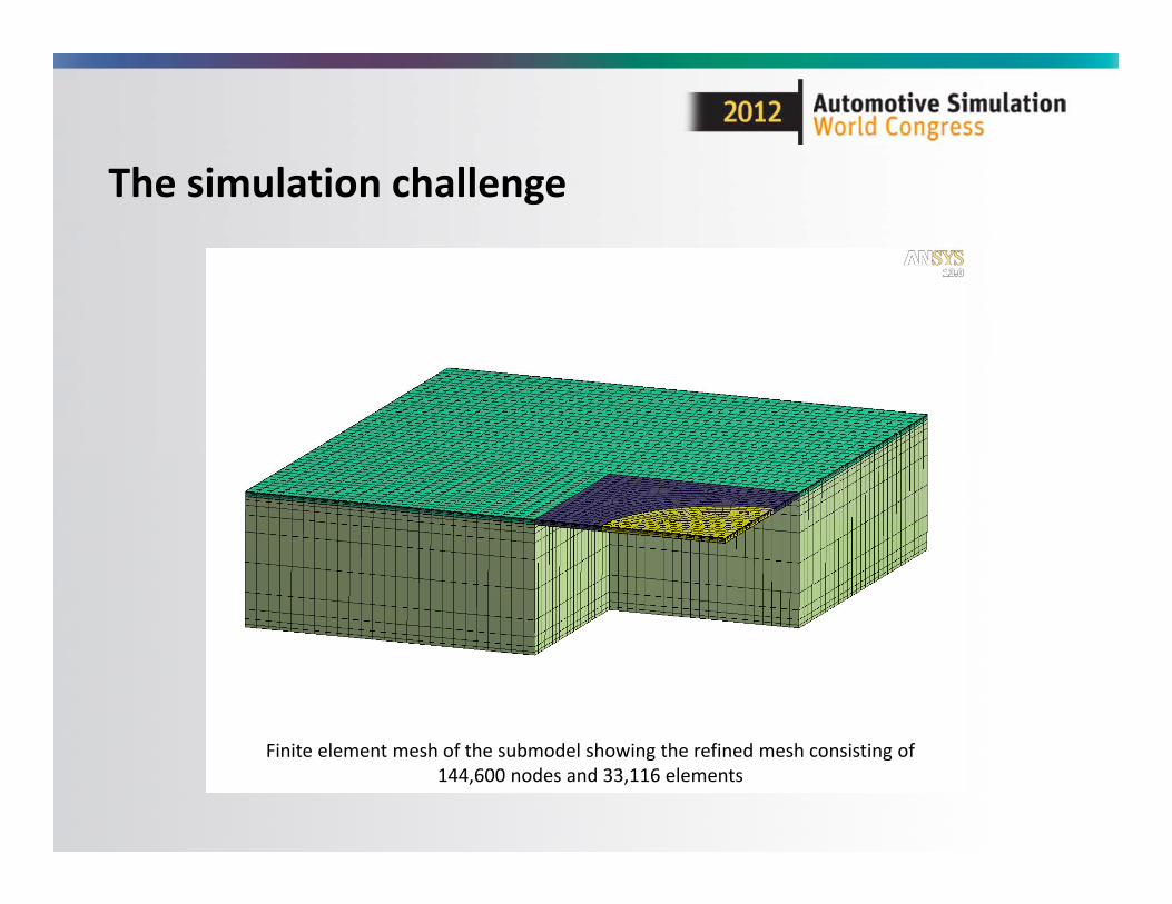
Finite element mesh of the submodel showing the refined mesh consisting of 144,600 nodes and 33,116 elements
Results
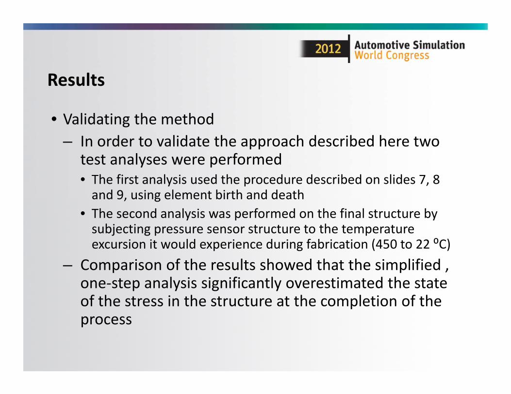
• Validating the method– In order to validate the approach described here two
test analyses were performed• The first analysis used the procedure described on slides 7, 8 and 9, using element birth and death
• The second analysis was performed on the final structure by subjecting pressure sensor structure to the temperature excursion it would experience during fabrication (450 to 22 ⁰C)
– Comparison of the results showed that the simplified , one‐step analysis significantly overestimated the state of the stress in the structure at the completion of the process
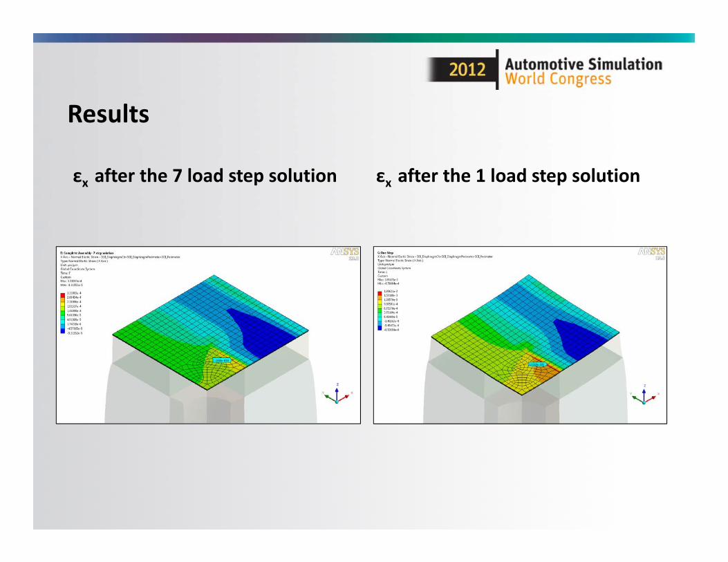
Results
εx after the 7 load step solution εx after the 1 load step solution

7.56
7.58
7.6
7.62
7.64
7.66
7.68
5
5.2
5.4
5.6
5.8
6
6.2
6.4
6.6
0 100 200 300 400 500 600 700 800
Deformation of the diaphragm [µ]
7‐Step Solution One‐Step Solution
Results
1 2
Results
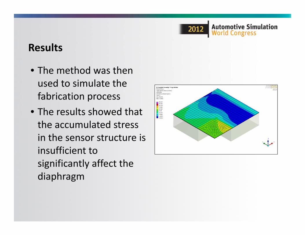
• The method was then used to simulate the fabrication process
• The results showed that the accumulated stress in the sensor structure is insufficient to significantly affect the diaphragm

Results
• The stressed substructure of the sensor was then used to model the behavior of the sensor when subjected to various pressure levels
Summary
• Element birth and death and submodeling were used to simulate the fabrication of an all silicon pressure sensor
• This approach allowed elimination of residual stresses as a potential contributor to failure of the diaphragms
• The approach also showed that the alternative one‐step approach significantly overestimates the residual stresses in the sensor
• The resulting model was successfully used to simulate the behavior of the sensor under various pressure levels


![Design of MEMS Capacitive Pressure Sensor for Continuous ...piezoresistive sensing technique [1, 2]. Piezoresistive pressure sensor is preferred because the properties of silicon material](https://img.pdfslide.us/doc/110x75/60e791e2d9071929211c8912/design-of-mems-capacitive-pressure-sensor-for-continuous-piezoresistive-sensing.jpg)