Simulating Ductile Fracture in Steel using the FiniteElement Method: Comparison of Two Models For

Describing Local Instability due to Ductile Fracture.

by

Henning Levanger

THESISfor the degree of

MASTER OF SCIENCE(Master i Anvendt matematikk og mekanikk)

Faculty of Mathematics and Natural SciencesUniversity of Oslo

May 2012

Det matematisk- naturvitenskapelige fakultetUniversitetet i Oslo

ii

Foreword

This thesis is written for the degree of Master of Science at the University of Oslo,Department of Mathematics, Mechanics division. The work has been done in col-laboration with Det Norske Veritas, in the Ship Structure and Concepts section ofthe Maritime Advisory department, and has been carried out at their main officeat Høvik, Oslo.

The topic of the thesis originates from the desire of group leader Eivind Steen toinvestigate the field of fracture mechanics and related theory and methods. Itsmain goal is to develop a better understanding of how to use the finite elementmethod to simulate collision events and damage caused by dropped objects, andhow to compute a structure’s resistance and the amount of damage inflicted bysuch an events. The focus of the thesis has been on the event of ductile fracture ofmetal, particularly steel, and the use of two different models for simulating ductilefracture behavior using the finite element method. During the work on the thesis Ihave learned a lot about the subject of fracture mechanics, a subject I did not haveany insight into before I began this work. I have also learned a great deal fromfiddling with the FE-analysis software ABAQUS, and spent many hours learningand understanding how to use the finite element method in the context of mywork.

I would like to thank Lars Brubak and Eivind Steen for giving me the opportu-nity to collaborate with their section while working on the thesis, and especiallyLars Brubak for helping me as my supervisor both at DNV and at the university.I would also like to thank Gabriele Notaro, for sharing his experience on usingthe finite element method and ABAQUS to simulate collision events, and for themany hours of guidance and discussions of the different results and choices thathave been made during the last year. I would also like to thank Tom KlungsethØsvold for sharing his opinions on some of the problems that I have encounteredduring this year. Thanks to Helene Lo Casico Sætrefor proofreading, and last, butdefinitely not least, a great thank you to my girl-friend Ingrid Senje Rasmussen forgreat moral support and for the help with proofreading the thesis.

iii

iv

Abstract

In the shipping industry, there is an increase in the requirement of determining aship’s strength when it comes to collision events. This involves ship-against-shipcollisions, but also strength against damage caused by dropped objects, groundingevents and collision with rigid objects. There are many methods of determiningthe damage inflicted to the structure when two objects collide. The most advancedones make use of numerical methods and particularly the finite element method.

This thesis gives an overview of the theory involved in a ductile failure of anisotropic ductile material such as steel, and explains two different methods of mod-eling the material behavior related to ductile fracture for use in the finite elementmethod. One model uses the material’s true stress/true strain relationship to sim-ulate the structural response due to reduced load-bearing capacity form ductilefracture. The other is a complete fracture model that reduces the load bearing ca-pacity by inflicting damage to the elements used, and is based on the assumedamount of energy it takes to create a crack. The theory behind the two modelsis explained in this thesis, and material models are developed using a tensile testmodel in the finite element software package ABAQUS. Then the material mod-els developed are used on a model simulating a steel plate being penetrated bya cone shaped object. The results are compared to earlier material tests done onthe same type of structures. Both fracture models are capable of simulating theductile fracture of a tensile specimen, and no significant differences can be foundwhen monitoring the energy output. When the same material-definition modelsare used in an analysis of a plate being penetrated, it is however evident that thereare differences that are caused by the difference in the way the ductile fracture issimulated. Particularly the effect of reduced stiffness in the elements when us-ing the energy-based fracture model leads to the conclusion that the two methodsmake the FE-model behave differently when high values of in-plane tensile strainis present.

i

Contents

1 Introduction to the thesis 1

1.1 Introduction . . . . . . . . . . . . . . . . . . . . . . . . . . . . . . . . . 1

1.2 Specification of the thesis . . . . . . . . . . . . . . . . . . . . . . . . . . 2

1.3 Organization of the thesis . . . . . . . . . . . . . . . . . . . . . . . . . 3

2 Material Theory 4

2.1 The stress-strain curve . . . . . . . . . . . . . . . . . . . . . . . . . . . 4

2.2 Elasticity . . . . . . . . . . . . . . . . . . . . . . . . . . . . . . . . . . . 9

2.3 Plasticity . . . . . . . . . . . . . . . . . . . . . . . . . . . . . . . . . . . 11

2.4 Yield criterion . . . . . . . . . . . . . . . . . . . . . . . . . . . . . . . . 13

3 Fracture mechanics 16

3.1 Introduction to ductile fracture . . . . . . . . . . . . . . . . . . . . . . 16

3.2 Ductile Fracture . . . . . . . . . . . . . . . . . . . . . . . . . . . . . . . 18

3.2.1 Creation of voids . . . . . . . . . . . . . . . . . . . . . . . . . . 18

3.2.2 Void growth and coalescence . . . . . . . . . . . . . . . . . . . 21

3.2.3 Mathematic models for predicting the growth of voids andonset of fracture. . . . . . . . . . . . . . . . . . . . . . . . . . . 24

4 Fracture mechanic parameters 26

4.1 Introduction . . . . . . . . . . . . . . . . . . . . . . . . . . . . . . . . . 26

4.2 Stress parameters . . . . . . . . . . . . . . . . . . . . . . . . . . . . . . 27

4.2.1 the von Mises equivalent stress . . . . . . . . . . . . . . . . . . 27

ii

4.2.2 Hydrostatic stress/Pressure stress . . . . . . . . . . . . . . . . 29

4.2.3 Deviatoric stress . . . . . . . . . . . . . . . . . . . . . . . . . . 30

4.2.4 Stress Triaxiality . . . . . . . . . . . . . . . . . . . . . . . . . . 30

4.3 Strain parameters . . . . . . . . . . . . . . . . . . . . . . . . . . . . . . 32

4.3.1 Equivalent plastic strain . . . . . . . . . . . . . . . . . . . . . . 32

4.4 Other parameters related to yielding and fracture of ductile materials 33

4.4.1 Lode parameter and lode angle . . . . . . . . . . . . . . . . . . 33

4.4.2 Characteristic Element Length . . . . . . . . . . . . . . . . . . 34

5 Fracture models in the finite element method 38

5.1 Introduction . . . . . . . . . . . . . . . . . . . . . . . . . . . . . . . . . 38

5.2 A fracture model using the true stress/true strain relationship . . . . 41

5.2.1 Introduction . . . . . . . . . . . . . . . . . . . . . . . . . . . . . 41

5.2.2 Ehlers and Varsta plasticity model . . . . . . . . . . . . . . . . 42

5.3 Fracture model defining the fracture energy dissipated . . . . . . . . 46

5.3.1 Introduction . . . . . . . . . . . . . . . . . . . . . . . . . . . . . 46

5.3.2 Fracture model by Hillerborg et al. . . . . . . . . . . . . . . . . 48

6 Explicit dynamic analysis in FEM 51

6.1 Introduction . . . . . . . . . . . . . . . . . . . . . . . . . . . . . . . . . 51

6.2 Dynamic analysis using direct integration methods . . . . . . . . . . 51

6.3 Explicit analysis . . . . . . . . . . . . . . . . . . . . . . . . . . . . . . . 52

6.3.1 Central Difference Method . . . . . . . . . . . . . . . . . . . . 53

6.3.2 Stability . . . . . . . . . . . . . . . . . . . . . . . . . . . . . . . 54

6.3.3 Estimation of the stable time increment size . . . . . . . . . . . 55

6.3.4 Time reduction . . . . . . . . . . . . . . . . . . . . . . . . . . . 56

6.3.5 Energy monitoring . . . . . . . . . . . . . . . . . . . . . . . . . 56

6.4 Single versus double precision . . . . . . . . . . . . . . . . . . . . . . 57

iii

7 Tensile experiment in ABAQUS 58

7.1 Introduction . . . . . . . . . . . . . . . . . . . . . . . . . . . . . . . . . 58

7.2 The FE model . . . . . . . . . . . . . . . . . . . . . . . . . . . . . . . . 59

7.3 Development of the material models . . . . . . . . . . . . . . . . . . . 63

7.3.1 Plasticity-model (PMM) . . . . . . . . . . . . . . . . . . . . . . 64

7.3.2 Damage Evolution Material Model (DEMM) . . . . . . . . . . 65

7.4 Results and discussion . . . . . . . . . . . . . . . . . . . . . . . . . . . 67

7.4.1 The material models . . . . . . . . . . . . . . . . . . . . . . . . 67

7.4.2 Comparing energy components . . . . . . . . . . . . . . . . . 74

7.4.3 Fracture displacement and reduced strength . . . . . . . . . . 82

7.4.4 Final comments to the results . . . . . . . . . . . . . . . . . . . 86

8 Plate penetration experiment in ABAQUS 88

8.1 Introduction . . . . . . . . . . . . . . . . . . . . . . . . . . . . . . . . . 88

8.2 The model . . . . . . . . . . . . . . . . . . . . . . . . . . . . . . . . . . 89

8.3 Analysis . . . . . . . . . . . . . . . . . . . . . . . . . . . . . . . . . . . 93

8.4 Results and discussion . . . . . . . . . . . . . . . . . . . . . . . . . . . 95

8.4.1 Introduction . . . . . . . . . . . . . . . . . . . . . . . . . . . . . 95

8.4.2 The 17.6 mm meshed model . . . . . . . . . . . . . . . . . . . . 97

8.4.3 The 8.8 mm meshed model . . . . . . . . . . . . . . . . . . . . 99

8.4.4 The 2.2 mm and the 4.4 mm meshed model . . . . . . . . . . . 100

8.4.5 Reduction of structural strength . . . . . . . . . . . . . . . . . 106

9 Summary and conclusion 108

A Appendix A 111

A.1 Material Plasticity in Abaqus . . . . . . . . . . . . . . . . . . . . . . . 111

A.2 Damage Initiation Criteria . . . . . . . . . . . . . . . . . . . . . . . . . 113

A.2.1 Ductile criteria . . . . . . . . . . . . . . . . . . . . . . . . . . . 114

A.2.2 Shear criterion . . . . . . . . . . . . . . . . . . . . . . . . . . . . 115

iv

A.3 Damage evolution . . . . . . . . . . . . . . . . . . . . . . . . . . . . . . 115

v

List of Notations

A Cross-section areaA0 Initial cross-section areaD Damage parameterE Young modulusEAE ”Artificial” strain energyEDM Damage dissipated energyEFric Energy dissipated by friction effectsEInt Internal energyEKE Kinetic energyEPD Plastic deformation energyESE Elastic strain energyEUB Unbalanced energyF ForceG Shear modulusG f Energy dissipated to damage per unit area of crackK Stress intensity factorLσ Lode parameterS1, S1, S3 Principle deviatoric stresses.VV Void volumeWExt External workWPW Work done by the penalty contact definition[C] Dampening matrix[M] Mass matrixεpl Equivalent plastic strainε

plD Equivalent plastic strain at the point of damage initiation

upl Fracture displacementupl

f Fracture displacement at fracture.

vi

S Deviatoric stress tensoru Second derivative of displacement˙εpl Equivalent plastic strain rateεi Strain rateu First derivative of displacementη Deviatoric stress componentη Stress triaxialityγxy,γyz,γzx Shear strain componentsν Poisson’s ratioωmax Maximum natural frequencyρ Material densityσ Stressσ 1,σ 2,σ 3 Deviatoric components of the principle stressσ1,σ2,σ3 Principle stress (σ1 ≥ σ2 ≥ σ3)σc Interfacial stress. Stress acting across the interface of two different par-

ticlesσe von Mises equivalent stressσe von Mises equivalent stressσm Hydrostatic stressσu Ultimate strength stressσx,σy,σz Stress componentsσy Yield stressσY,lower Stress value at the lower yield pointσY,upper Stress value at the upper yield pointσeng The ”engineering” stress ( F

A )σi j Stress acting on the i plane in the direction of j.σtrue The true stress in the materialτxy, τyz, τzx Shear stress componentsθ Lode angleε Strainεel Elastic strainεpl elastic strainεx,εy,εz Strain componentsεeng Engineering strainεtot Total strain (εtot = εel +εpl)εtrue True/logarithmic strainξmax The dampening ratio for theωmax mode{Rext}n External load vector

vii

{Rint}n Internal load vector{u} Second derivative of displacement (acceleration){u} First derivative of displacement (velocity)cd Speed of sound in the materiall Initial lengthl Lengthlc charateristic element lengthle Element lengthlemin Smallest dimension of a elementp Equivalent hydrostatic pressuret timeu Displacement

viii

ix

Chapter 1

Introduction to the thesis

1.1 Introduction

In shipping, the forces involved when a collision takes place are enormous, andwill produce permanent deformations, cracks, local buckling, collapse and tearingof the ship structure. These damages may lead to flooding of the hull, stabilityproblems and possible progressive collapse of the ship’s structure. With smallerdamages, the ship’s stability may not be affected, but leakage of oil and fuel mayoccur, threatening the environment. The amount of damage caused by the collisionis crucial when the remaining strength of the hull is to be determined.

To better determine the amount of damage caused by a collision or grounding of aship, it is important to use a reliable deterministic analysis models. The most ad-vanced models are making use of the finite element method and non-linear analy-sis in computer assisted analysis, using software packages such as ABAQUS, AN-SYS and LS-DYNA. However, the quality of the solutions produced in these pro-grams when preforming an analysis is no better than the information inputted intothe model, and is dependent on a large number of parameters, particularly whentrying to simulate fracture and the development of cracks in the material. Theseparameters are essential for understanding, and having control over the results,when computing the extent of damage and the energy absorbed by the structure.

Det Norske Veritas has for the past few years been working to develop new and

1

more accurate methods and models to determine the energy and deformationcaused by collision forces. This has been done by evaluating different scenarios,including different hull designs, and using simplified methods of accidental limitstate analysis. DNV has developed the computer analysis program SIDECOLL/BOWCOLL which makes use of simplified methods. A more detailed approach isdesirable in order to calibrate and improve these simplified models against non-linear FE-analyses.

1.2 Specification of the thesis

The objective of this thesis is to find and validate the properties of a specified ma-terial to be used when performing a FE-analysis considering large deformationand ductile fracture of the material. The main objective is to identify different pa-rameters that may have an impact on a model’s ability to absorb energy during asimulated collision, and to make simplifications to the input data in order to sim-plify the modelling procedure. The materials that will be used are homogeneousisotropic ductile metals, as this is the material most used in ship structures of today.

The main focus of the thesis will be the material properties, and determining thefracture criteria related to the mesh size of the FE-model. It will also be perform acomparison of two different approaches to model the materials fracture behavior,and applicate them in the finite element method. A tensile test experiment will beperformed using the finite elements software package ABAQUS, in order to de-velop material models for two different theories to model fracture. These materialmodels will then be used to simulate a plate being penetrated by an object at lowspeed. The goal is to determine the different material models’ ability to simulatethe fracturing of the material, and to compare the models against each other. Thethesis is limited to ductile fracturing of isotropic homogeneous ductile materials.

The theory regarding the topics above will be studied and presented as an intro-duction into the science of material fracture, and how these theories are imple-mented into the finite element method.

2

1.3 Organization of the thesis

The thesis is divided into nine chapters. The first chapter is an introduction to thethesis and the work done to prepare it. Chapter 2 contains theory about mate-rial behavior for mechanical loads and in the third the material theory of fracturefor ductile fracturing is presented. The fourth chapter explains some of the ma-terial parameters that are of interest when ductile fracturing is studied. Chapter5 introduces the two material models to be used in the experiments carried outduring the work of the thesis. The sixth chapter explaines the explicit time inte-gration method used in the finite element analysis in the subsequent chapters. InChapter 7 a tensile experiment performed using the finite element software anal-ysis program ABAQUS is presented, and the results are discussed. The main goalof this experiment is to develop material models in to be used in ABAQUS fordynamic analysis of a forced penetration of a steel plate specimen. The penetra-tion experiment is presented in Chapter 8, and the results regarding the use of thetwo material models developed as well as the results related to the fracturing ofthe plate are discussed. In Chapter 9 the results and findings are discussed, and aconclusion is made.

3

Chapter 2

Material Theory

2.1 The stress-strain curve

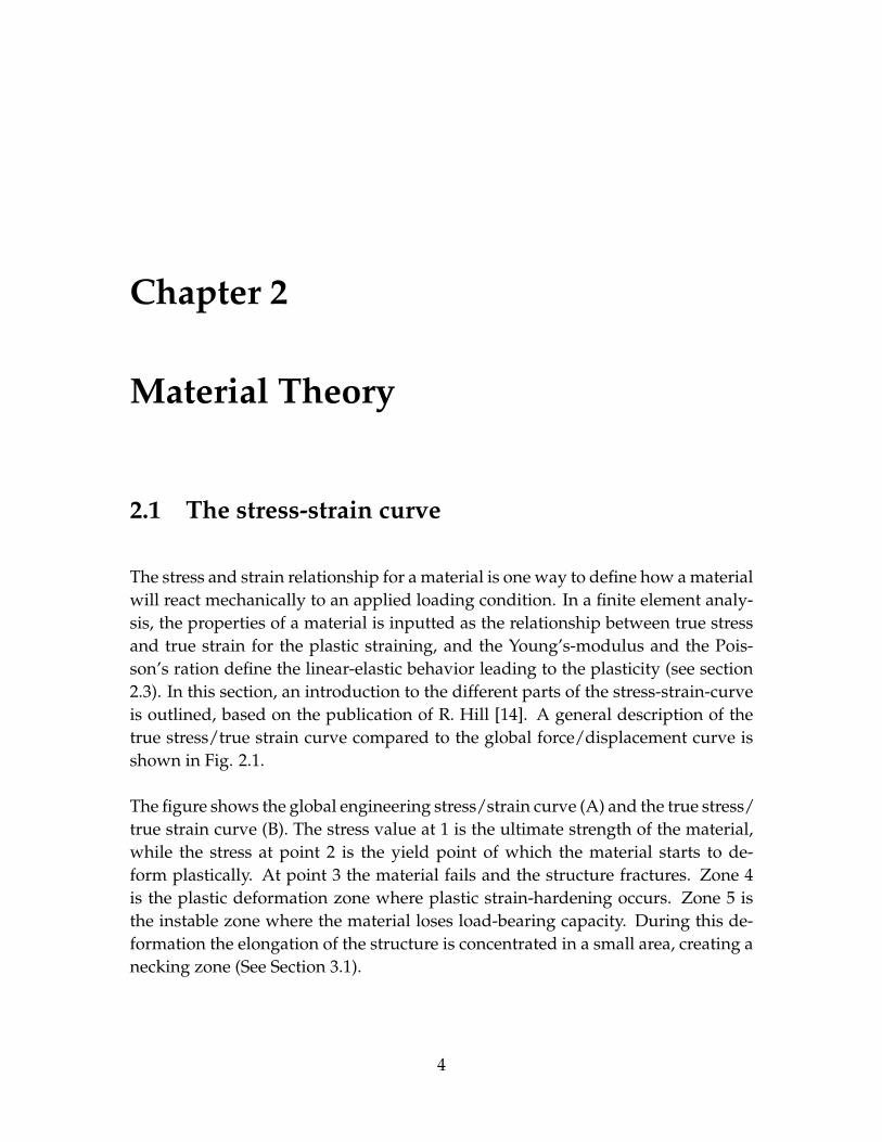
The stress and strain relationship for a material is one way to define how a materialwill react mechanically to an applied loading condition. In a finite element analy-sis, the properties of a material is inputted as the relationship between true stressand true strain for the plastic straining, and the Young’s-modulus and the Pois-son’s ration define the linear-elastic behavior leading to the plasticity (see section2.3). In this section, an introduction to the different parts of the stress-strain-curveis outlined, based on the publication of R. Hill [14]. A general description of thetrue stress/true strain curve compared to the global force/displacement curve isshown in Fig. 2.1.

The figure shows the global engineering stress/strain curve (A) and the true stress/true strain curve (B). The stress value at 1 is the ultimate strength of the material,while the stress at point 2 is the yield point of which the material starts to de-form plastically. At point 3 the material fails and the structure fractures. Zone 4is the plastic deformation zone where plastic strain-hardening occurs. Zone 5 isthe instable zone where the material loses load-bearing capacity. During this de-formation the elongation of the structure is concentrated in a small area, creating anecking zone (See Section 3.1).

4

Figure 2.1: Global responce of the material (A) and the local true stress/true strain relationship (B)for the same material.

In order to determine a material’s mechanical properties, it is usually put throughmechanical tests where different parameters are measured. Normal test meth-ods are tensile tests of flat-bars or rods, compression of a short cylindrical blockor twisting of a thin-walled tube. The force applied and the deformation that isproduced can be used to calculate the internal stress in the material and the totalstraining of the material. The internal stress σ , and the true strain εtrue and theengineering strain εeng of the material can be calculated as

σ =FA

(2.1)

εtrue = ln(ll0) = ln(1 +εeng) (2.2)

εeng =l − l0

l0(2.3)

.

A is the deformed cross-section area, F is the external applied force, εtrue is thelogarithmic strain or true strain, and εeng is the engineering strain or conventionalstrain. For small values of strain, the two different strain measurements are ap-proximately equal, but for higher strain values εtrue develops significantly higherstrain values because of the logarithmic development, while εeng develops in a lin-early manner. The relative difference in strain value can be seen in Fig. 2.2. This

5

way of measuring the strain in a structure depending on the global elongation ofthe material, is only valid as long as there are no local instabilities present in thematerial.

Elongation [mm]

Total length [mm]

0.1 0.2 0.3 0.4 0.5 0.6 0.7 0.801.0

1.1

1.2

1.3

1.4

1.5

1.6

1.7

1.8

Figure 2.2: The difference between logarithmic strain εtrue (dashed curve) and engineering strainεeng (solid line). For small values of strain, the two different strains are as good as equal, but forstrain values above 2-3 % the difference may become significant depending on the case studied.

6

stress

strain

P

Y

U

py

u

O oo'

p'

u'

y'

Figure 2.3: The loading path of a material is plotted as stress against strain. P and p’ mark theproportional point for initial loading and reloading respectively. Y and y’ are the initial loadingyield point and reloaded yield point, the limit between elastic and elasto-plastic material behavior.O is the initial state, while o’ is the state after the material has be loaded up to point U. The distanceOo’ is the plastic deformation obtained by this load cycle. The small curve in the unloading pathtowards o’.

When a tensile specimen is subjected to an increasing load, it will respond by elon-gating. At first, the material will elongate in a linearly-elastic manner, followingHooke’s law (Section 2.2). The stress and strain will increase linearly dependenton each other, up to the proportional point P, in Fig. 2.3. At this point, the stress-strain relation stops being linearly dependent according to Hooke’s law, but inmost cases the strain is still elastic up to point Y. At the point of yielding Y, themaximum elastic strain εel

max is reached. Any further straining of the material willresult in plastic deformation and energy dissipated to permanent deformation ofthe material.

After the yielding point, the stress-strain curve starts to flatten out. For most duc-tile materials, an incremental increase in stress δσ will produce a progressivelylarger increase in strain δε, meaning that the slope of the curve is decreasing. Thisis the effect of strain-hardening in the material making it tougher as the strainincreases. If the specimen at some random point U (Fig. 2.3) during the plasticdeformation is being unloaded until the internal stress is zero, the strain responsewill drop following the slope defined by the Young’s modulus. A perfect materialwill follow this path down to a value of zero stress. At the end of unloading, the

7

curve may however bend off right before the stress reaches zero (in Fig. 2.3 thebend is highly exaggerated). This effect is due to some grains in the material beingorientated in such a way that they produce a very small amount of plastic strain.This small amount of strain energy is released some time after the external load isremoved, and the result is that the material is not fully contracted before the loadhas been removed for some time [14]. The difference in strain value between Oand o’ in the figure is the plastic elongation caused by the plastic straining of thematerial.

When the load is applied once more, the material will elongate in an elastic manneronce more, following Hooke’s law from point o’ up to the new proportional pointp’, and the yield at point y’. The yield point y is reached at a higher value of stressthan the first yield point Y, because of the pre-straining of the material before theload is applied for a second time. The yield point y can be considered as the yieldpoint for a material specimen that is pre-strained to a value of εpl

pre equal to thestrain value defined by the distance between O and o’.

During the plastic deformation of the material, the material increases its load bear-ing capacity per unit cross-section area, as a result of the strain hardening effect. Atthe same time, the effective cross-section is reduced due to transverse contractionas the material is stretched. The stress/strain curve will rise as long as the strain-hardening is increasing faster than the cross-section area is decreasing, meaningthat δσ/δε < σ , where σ is the true stress in the material. The decreasing slope inthe stress/strain curve is caused by the δσ getting smaller compared to δε. At somepoint during the plastic straining of the material, the increase in strain-hardeningwill be overcome by the cross-section area reduction. At this point the maximumload that the structure can carry is applied. The point is defined to be when [24]

dσdε

= σ (2.4)

where σ is the current true stress value. Any further straining of a material willintroduce a local instability in the material, leading to an even more reduced loadbearing capacity and eventually fracture. This is explained in more detail in Sec.3.1.

8

2.2 Elasticity

A material will behave elastically if the strain energy that is built up in the materialis recoverable when the material is unloaded. When a force F is acting on a pieceof material giving a displacement ∆l, it will exert an external work which equalsWE = F∆l. It is assumed that all of the external energy is used to produce thedeformation ∆l, and that the kinetic energy and energy lost to friction forces arenegligible. If so, the external energy will be matched by the internal energy, andthe internal energy is equal to the elastic strain energy in the volume.

WExt = EInt = ESE (2.5)

WE is the external work, EInt is the internal energy and ESE is the elastic strainenergy in the material.

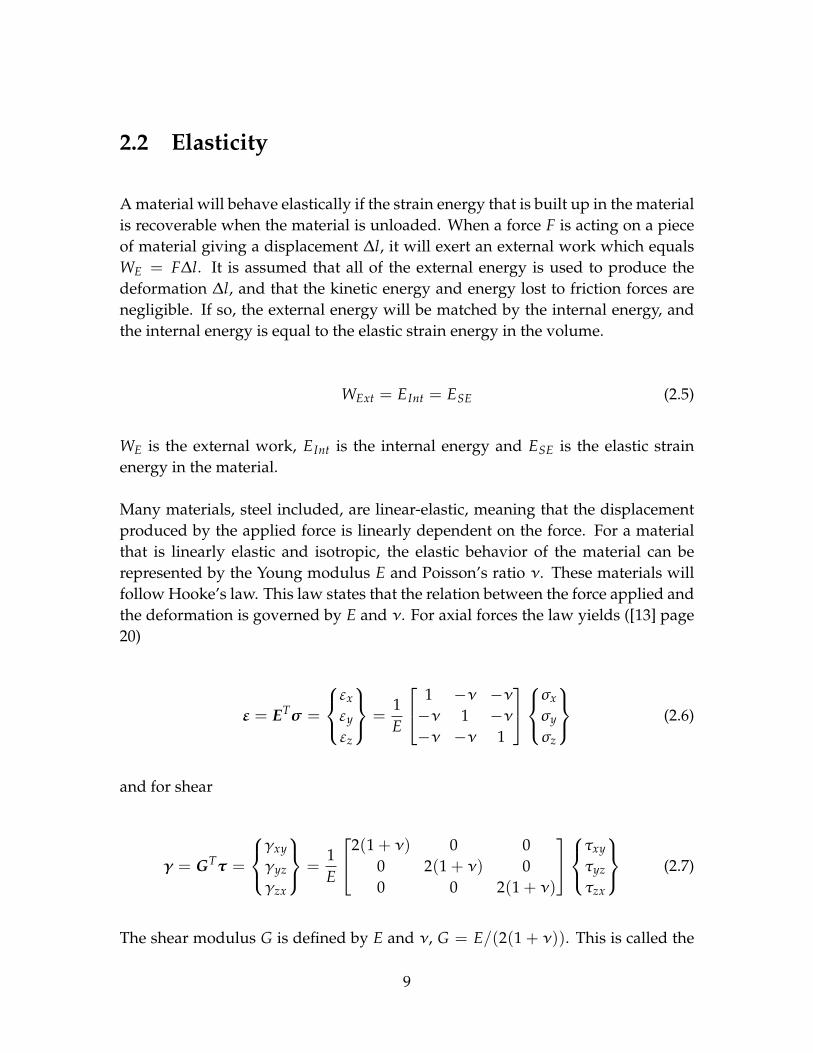
Many materials, steel included, are linear-elastic, meaning that the displacementproduced by the applied force is linearly dependent on the force. For a materialthat is linearly elastic and isotropic, the elastic behavior of the material can berepresented by the Young modulus E and Poisson’s ratio ν. These materials willfollow Hooke’s law. This law states that the relation between the force applied andthe deformation is governed by E and ν. For axial forces the law yields ([13] page20)

ε = ETσ =

εx

εy

εz

=1E

1 −ν −ν−ν 1 −ν−ν −ν 1

σx

σy

σz

(2.6)

and for shear

γ = GTτ =

γxy

γyz

γzx

=1E

2(1 + ν) 0 00 2(1 + ν) 00 0 2(1 + ν)

τxy

τyz

τzx

(2.7)

The shear modulus G is defined by E and ν, G = E/(2(1 + ν)). This is called the

9

full Hooke’s law for 3D-space.

Figure 2.4: A beam with an applied force F resulting in a internal stress of σ = F/A and aelongation ∆l.

Considering a simple structure like the rod in Fig. 2.4, the relation between elon-gation and strain, and applied force F and internal stress σ becomes apparent.

σ =FA

(2.8)

The strain value in the material is determined as

εeng =l0 + ∆l

l0(2.9)

where l0 is the initial length and δl is the elongation of the material.

As long as the material is acting elastically, all of the strain energy is recoverableand the material will obtain its original shape and size if the force F is removed.In a real structure, some of the energy applied to the structure may be lost throughe.g. heat. These effects are often neglected when studying structures loaded inthe elastic region, because the amount of energy lost through them is small. In ahigh speed impact, there will also be a significant amount of energy dissipated todynamic damping and the inertia of mass. These kinds of scenarios usually bringthe material into high levels of plastic strain deformation, and the dynamic effectsare small during the time the material is acting in an elastic manner.

For cases where ductile fracture of a material is studied, the elastic behavior of thematerial is of less importance during loading because the fracture strains are muchlarger than the elastic yield strain of the material. Normally, the maximum elasticstrain value for steel is about 2− 3 ‰, while the fracture strain is around 20− 24% defined in engineering strain εeng. In an analysis where fracture is studied, thedeformation of the material is much larger than what the elastic strain can produce,

10

and therefore it is not of great importance how the material behaves in the elasticarea when the deformation is increasing. For unloading of a structure that hasbeen loaded beyond the point of ultimate strength (referring to Fig. 2.1) the elasticproperties of the material are important. These are discussed in more detail insection 2.3.

2.3 Plasticity

When the material deforms according to its elastic properties, the strain energyapplied is recoverable. When the stress in the material reaches the yield point, themaximum elastic strain εel

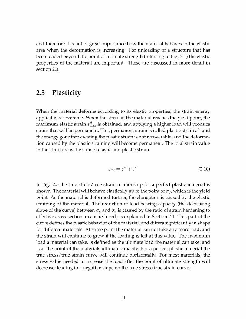
max is obtained, and applying a higher load will producestrain that will be permanent. This permanent strain is called plastic strain εpl andthe energy gone into creating the plastic strain is not recoverable, and the deforma-tion caused by the plastic straining will become permanent. The total strain valuein the structure is the sum of elastic and plastic strain.

εtot = εel +εpl (2.10)

In Fig. 2.5 the true stress/true strain relationship for a perfect plastic material isshown. The material will behave elastically up to the point ofσy, which is the yieldpoint. As the material is deformed further, the elongation is caused by the plasticstraining of the material. The reduction of load bearing capacity (the decreasingslope of the curve) between σy and σu is caused by the ratio of strain hardening toeffective cross-section area is reduced, as explained in Section 2.1. This part of thecurve defines the plastic behavior of the material, and differs significantly in shapefor different materials. At some point the material can not take any more load, andthe strain will continue to grow if the loading is left at this value. The maximumload a material can take, is defined as the ultimate load the material can take, andis at the point of the materials ultimate capacity. For a perfect plastic material thetrue stress/true strain curve will continue horizontally. For most materials, thestress value needed to increase the load after the point of ultimate strength willdecrease, leading to a negative slope on the true stress/true strain curve.

11

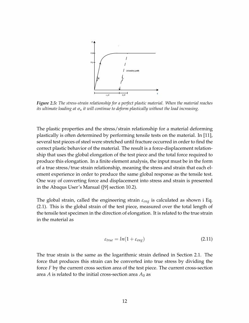
Figure 2.5: The stress-strain relationship for a perfect plastic material. When the material reachesits ultimate loading at σu it will continue to deform plastically without the load increasing.

The plastic properties and the stress/strain relationship for a material deformingplastically is often determined by performing tensile tests on the material. In [11],several test pieces of steel were stretched until fracture occurred in order to find thecorrect plastic behavior of the material. The result is a force-displacement relation-ship that uses the global elongation of the test piece and the total force required toproduce this elongation. In a finite element analysis, the input must be in the formof a true stress/true strain relationship, meaning the stress and strain that each el-ement experience in order to produce the same global response as the tensile test.One way of converting force and displacement into stress and strain is presentedin the Abaqus User’s Manual ([9] section 10.2).

The global strain, called the engineering strain εeng is calculated as shown i Eq.(2.1). This is the global strain of the test piece, measured over the total length ofthe tensile test specimen in the direction of elongation. It is related to the true strainin the material as

εtrue = ln(1 +εeng) (2.11)

The true strain is the same as the logarithmic strain defined in Section 2.1. Theforce that produces this strain can be converted into true stress by dividing theforce F by the current cross section area of the test piece. The current cross-sectionarea A is related to the initial cross-section area A0 as

12

A = A0l0

l(2.12)

and inserting this into the force-stress relation σ = F/A gives

σtrue =FA

=Fl

A0l0= σeng

ll0

(2.13)

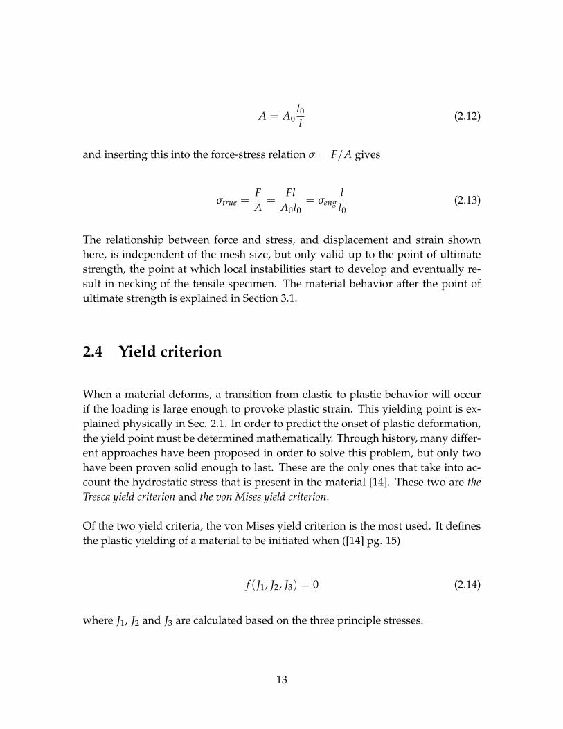
The relationship between force and stress, and displacement and strain shownhere, is independent of the mesh size, but only valid up to the point of ultimatestrength, the point at which local instabilities start to develop and eventually re-sult in necking of the tensile specimen. The material behavior after the point ofultimate strength is explained in Section 3.1.

2.4 Yield criterion

When a material deforms, a transition from elastic to plastic behavior will occurif the loading is large enough to provoke plastic strain. This yielding point is ex-plained physically in Sec. 2.1. In order to predict the onset of plastic deformation,the yield point must be determined mathematically. Through history, many differ-ent approaches have been proposed in order to solve this problem, but only twohave been proven solid enough to last. These are the only ones that take into ac-count the hydrostatic stress that is present in the material [14]. These two are theTresca yield criterion and the von Mises yield criterion.

Of the two yield criteria, the von Mises yield criterion is the most used. It definesthe plastic yielding of a material to be initiated when ([14] pg. 15)

f (J1, J2, J3) = 0 (2.14)

where J1, J2 and J3 are calculated based on the three principle stresses.

13

J1 = σ1 +σ2 +σ3 (2.15)

J2 = −(σ1σ2 +σ2σ3 +σ3σ1) (2.16)

J3 = σ1σ2σ3 (2.17)

f is a characteristic value for the state of the material regarding plastic yielding.

In order to reduce the complexity of the yield criterion, it is assumed that the yieldof a material is unaffected by moderate- hydrostatic pressure and tension. An othersimplification is to eliminate the Bauschinger effect1so that the yield criterion is thesame for compression- and tension stress states. By making these assumptions, ithas been shown [14] that the yield criterion only depends on the principal com-ponents of the deviatoric stress tensor2(σ 1,σ 2,σ 3), and that the yield criterion isreduced to

F( J2) = 0 (2.18)

The J2 is called the second deviatoric stress invariant, and is defined as

J2 =12

Si jS ji (2.19a)

=16

[(σx −σy)

2 + (σy −σz)2 + (σz −σx)

2]+σ2

xy +σ2yz +σ

2xz (2.19b)

=16

[(σ1 −σ2)

2 + (σ2 −σ3)2 + (σ3 −σ1)

2]

(2.19c)

The deviator stress tensor Si j is defined in Section 4.2.3.

1The Bauschinger effect is an effect occurring in some materials, which link the maximum yieldstress for tensile loading to the yield stress for compressive loading. If e.g. the tensile yield stresslimit is increased, the compressive yield stress limit is equally reduced.

2Deviatoric stress is the stress that acts on a body giving changes only in the shape of the solidvolume, and not in the volume. The hydrostatic stress is the stress forces responsible for changingthe volume of the body. The real stress state is the sum of the hydrostatic and the deviatoric stressstates in the body ([6] pg. 609).

14

In practical use, the von Mises yield criterion is said to be fulfilled when the equiv-alent von Mises stressσe (defined in Section 4.2.1) is equal to the set yield stressσY([2] pg. 67) defined by

σY =

√2√23

k (2.20)

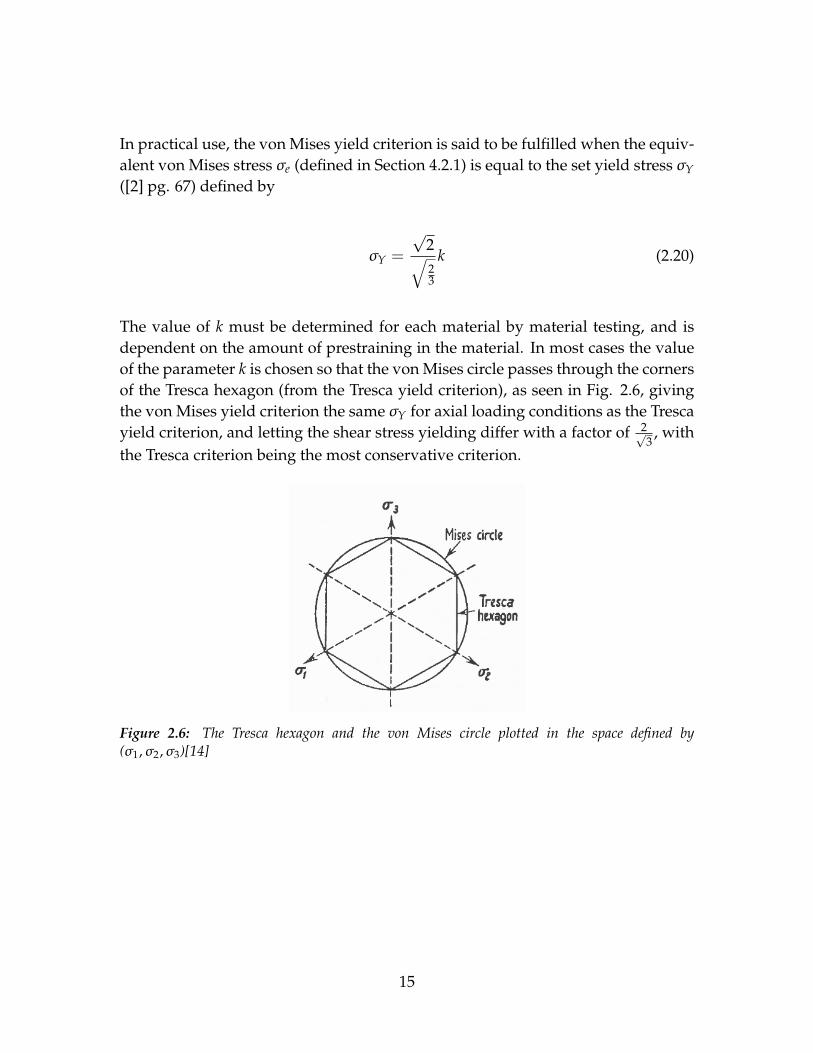
The value of k must be determined for each material by material testing, and isdependent on the amount of prestraining in the material. In most cases the valueof the parameter k is chosen so that the von Mises circle passes through the cornersof the Tresca hexagon (from the Tresca yield criterion), as seen in Fig. 2.6, givingthe von Mises yield criterion the sameσY for axial loading conditions as the Trescayield criterion, and letting the shear stress yielding differ with a factor of 2√

3, with

the Tresca criterion being the most conservative criterion.

Figure 2.6: The Tresca hexagon and the von Mises circle plotted in the space defined by(σ1,σ2,σ3)[14]

15

Chapter 3

Fracture mechanics

3.1 Introduction to ductile fracture

In section 2.1 the definition of the point of ultimate strength is explained. When thematerial reaches this point, an increase in loading will make the true (plastic) strainincrease drastically, and even if the load is reduced, the strain will increase. Thisphenomenon can be explained by the ratio of strain hardening not increasing thestrength of the material sufficiently to overcome the loss of load carrying capacitybecause of the decreasing cross-section area. After the point of ultimate strengthfor the material, the ratio of change in true stress to change in true strain is

δσtrue

δεtrue< σtrue (3.1)

When the material deforms plastically, the true strain in the material is approxi-mately equal through the specimen. As the ultimate strength is reached, all partsof the material are strained to the material’s maximum tensile strength. Some placein the material there will be a weak zone, that will not be able to carry the loadingapplied. In this zone, the ductile fracture will start to develop. The loading willcause the weaker area to strain further than the rest of the model, even if the load isnot increased. The increased straining in the small part of the specimen makes thematerial weaker in this area, which reduces the load bearing capacity of the speci-

16

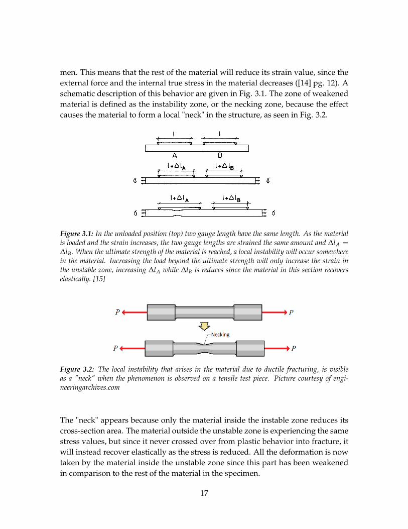
men. This means that the rest of the material will reduce its strain value, since theexternal force and the internal true stress in the material decreases ([14] pg. 12). Aschematic description of this behavior are given in Fig. 3.1. The zone of weakenedmaterial is defined as the instability zone, or the necking zone, because the effectcauses the material to form a local "neck" in the structure, as seen in Fig. 3.2.

Figure 3.1: In the unloaded position (top) two gauge length have the same length. As the materialis loaded and the strain increases, the two gauge lengths are strained the same amount and ∆lA =∆lB. When the ultimate strength of the material is reached, a local instability will occur somewherein the material. Increasing the load beyond the ultimate strength will only increase the strain inthe unstable zone, increasing ∆lA while ∆lB is reduces since the material in this section recoverselastically. [15]

Figure 3.2: The local instability that arises in the material due to ductile fracturing, is visibleas a "neck" when the phenomenon is observed on a tensile test piece. Picture courtesy of engi-neeringarchives.com

The "neck" appears because only the material inside the instable zone reduces itscross-section area. The material outside the unstable zone is experiencing the samestress values, but since it never crossed over from plastic behavior into fracture, itwill instead recover elastically as the stress is reduced. All the deformation is nowtaken by the material inside the unstable zone since this part has been weakenedin comparison to the rest of the material in the specimen.

17

3.2 Ductile Fracture

3.2.1 Creation of voids

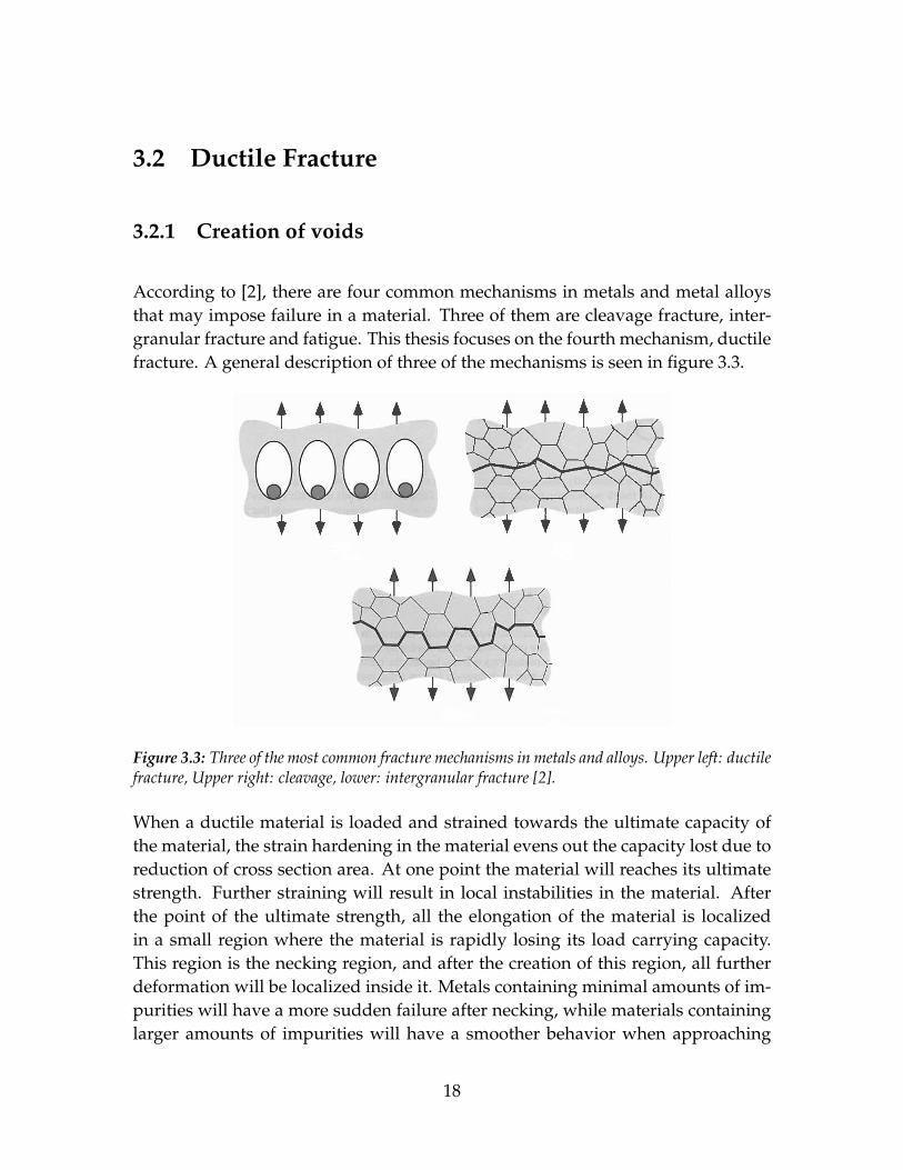
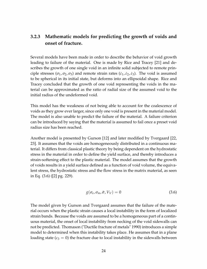
According to [2], there are four common mechanisms in metals and metal alloysthat may impose failure in a material. Three of them are cleavage fracture, inter-granular fracture and fatigue. This thesis focuses on the fourth mechanism, ductilefracture. A general description of three of the mechanisms is seen in figure 3.3.

Figure 3.3: Three of the most common fracture mechanisms in metals and alloys. Upper left: ductilefracture, Upper right: cleavage, lower: intergranular fracture [2].

When a ductile material is loaded and strained towards the ultimate capacity ofthe material, the strain hardening in the material evens out the capacity lost due toreduction of cross section area. At one point the material will reaches its ultimatestrength. Further straining will result in local instabilities in the material. Afterthe point of the ultimate strength, all the elongation of the material is localizedin a small region where the material is rapidly losing its load carrying capacity.This region is the necking region, and after the creation of this region, all furtherdeformation will be localized inside it. Metals containing minimal amounts of im-purities will have a more sudden failure after necking, while materials containinglarger amounts of impurities will have a smoother behavior when approaching

18

failure, but start to fail at lower values of strain. The mechanisms related to ductilefracture can generally be summed up into three stages ([2] page 219):

1. The formation of free surfaces around a particle inside the material, either byinterfacial decohesion or fracture in the particle itself.

2. Growth of the voids created around particles, due to plastic straining andhydrostatic stress.

3. Coalescence of the growing voids that eventually leads to failure of the ma-terial.

Some materials have strong bonds between the particles in the material, and thesematerial’s properties regarding ductile fracture is controlled by the developmentof voids around the particle. The strong bonds are usually caused by the materialhaving particles that are relatively uniform in size. When the voids first start toappear, the stress inside the material is so great that the growth and coalescence ofvoids happens quickly. This gives a material that is identified by a small amountof straining from the point of ultimate strength and to fracture. Other materialswhere the bonding between particles is weaker, usually because of larger differ-ences in size between particles, the voids easily develops around the large particle.The development of fracture is controlled by the growing and coalescence of thevoids around the larger particles that are evenly spread, but have a great distancesbetween them. This gives a material with a softer fracture behavior, but with largefracture straining, from ultimate strength to fracture.

Voids tend to appear around inclusions and so-called second-face particles thatmay be in the material. What happens is that the stress between the material matrixand the surface of the particle increases until the interfacial surface starts to slipand a void is created between the particle and the material matrix. It may alsooccur that the stress is so great that the particle itself fractures, splitting into partsand creating voids when it is pulled apart by the surrounding material.

Several models have been presented in order to define the stress causing the for-mation of voids. A widely used model presented in [2] and developed by A.S.Argon et al., states that the stress between the surface of a cylindrical particle andthe material matrix is approximately the sum of the equivalent von Mises stressand the hydrostatic stress in the material. This gives

19

σc = σe +σm (3.2)

where σc is the stress acting across the interface between a particle and the ma-terial matrix surrounding it, σe is the von Mises equivalent stress, and σm is thehydrostatic stress.

Later, this model has been redefined by The Beremin research group ([2] page 221)in order to make it better at predicting the right stress value when the productionof the material may lead to different directional properties due to rolling direction:

σc = σm + C(σe −σY) (3.3)

C is a parameter that is 0.6 for loading transverse to the rolling direction of thematerial, and 1.6 when loaded parallel to it. σY is the yield stress of the material.

Both these models use the equivalent von Mises stress and the hydrostatic stressin order to define the stress responsible for the creation of material voids.

A third model is developed by Goods and Brown ([2] page 221). They argue thatsmall dislocations near the surface of the particle will increase the stress valuearound the particle by

∆σd = 5.4αG

√ε1b

r(3.4)

α is a constant ranging from 0.14 to 0.33, G is the shear modulus, ε1 is the max-imum remote normal strain, b is the magnitude of Burger’s vector and r is theradius of the particle. They then define the interfacial stress σc to be

σc = ∆σd +σ1 = ∆σd + S1 +σm (3.5)

where σ1 is the maximum principle stress in the material and S1 is the maximumdeviatoric stress.

20

This latest model states that a material containing large particles will have a lowerdecohesion stress value because the larger radius of the particle means a lowervalue of ∆σd. Later studies have shown that the opposite is more likely to be true.Larger particles have an increased probability of having faults in them, makingthem more prone to fracture and therefore more likely to fail at a lower stress load-ing 1.

3.2.2 Void growth and coalescence

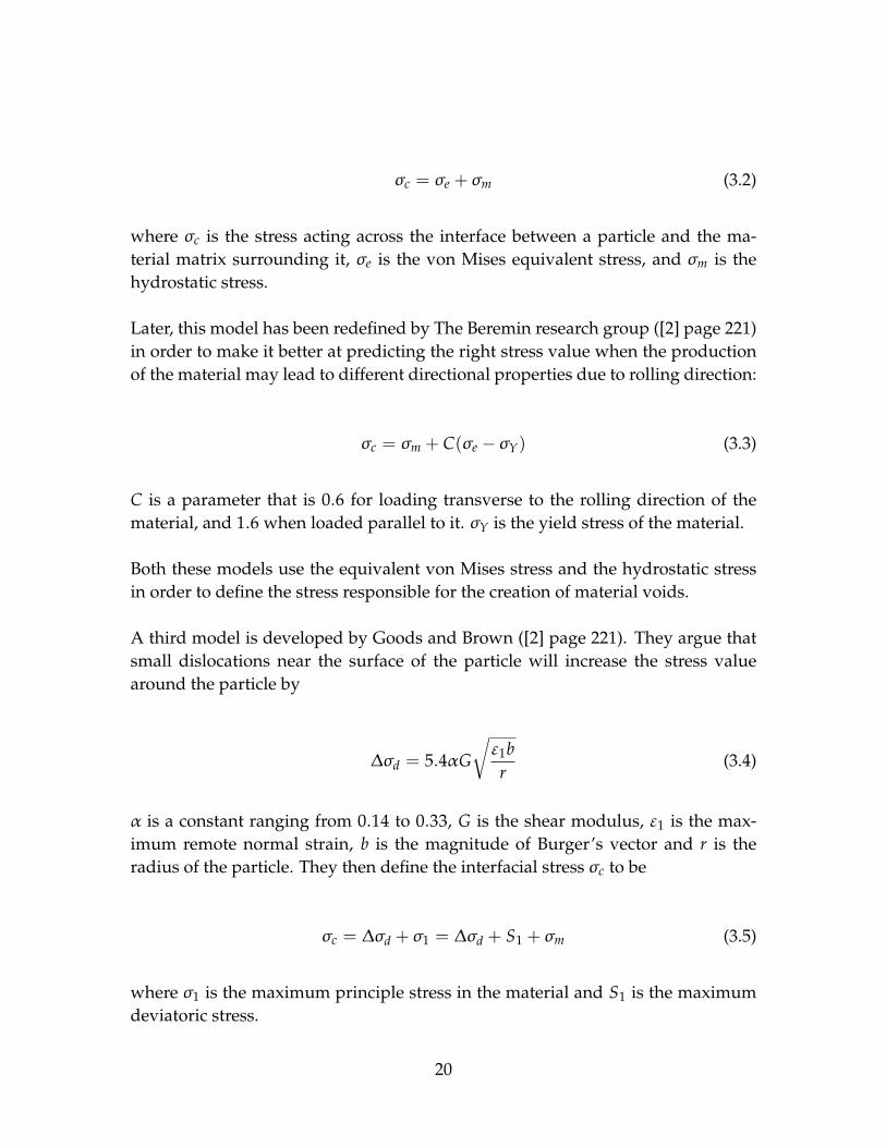
After the creation of voids in a material, these voids start to grow and coalesce asthe load on the material increases. Before the voids are created, the stress in thematerial is carried by the cross-section area of the specimen. As voids are created,the effective cross-section that can carry the load is reduced, since only the materialbetween the voids is available to carry it. The plastic straining resulting from theincreasing elongation is concentrated in the walls between the voids. It is thiseffect that causes the necking phenomenon of the material. In Fig. 3.4 a schematicdescription of the void growth and coalescence are shown.

The growth of voids is governed by the increasing plastic strain and the hydrostaticstress that acts on the material. In a specimen exposed to straining, the volumeat the center of the cross-section area carrying the load will experience a higheramount of hydrostatic stress than the volume closer to the edge. This higher hy-drostatic stress results in a higher state of stress triaxiality (Hydrostatic stress andstress triaxiality are explained in Chapter 4) in the center of the cross-section area.This will increase the speed at which the voids around the larger particles grow,and make the center of the loaded cross-section area fail before the edges ([2] pg.223). The shape of the center fracture caused by the growth of voids around thelarger particles, is often circular shaped. (In a flat-bar specimen the circular shapeis compromised by the shape of the specimens cross-section area)

Outside the center fracture zone, the stress triaxiality has a lower value becausethe hydrostatic stress is smaller. This has promoted the growth of smaller voidsaround the smaller particles, resulting in a lower maximum amount of strain fromultimate strength to fracture. When suddenly all of the loading is put onto this area

1In a short article by Jay R. Lund and Joseph P. Bryne [19] the theory behind the fact that largerbodies of mass are more prone to material weakness is pointed out based on an experiment per-formed by Leonardo da Vinci.

21

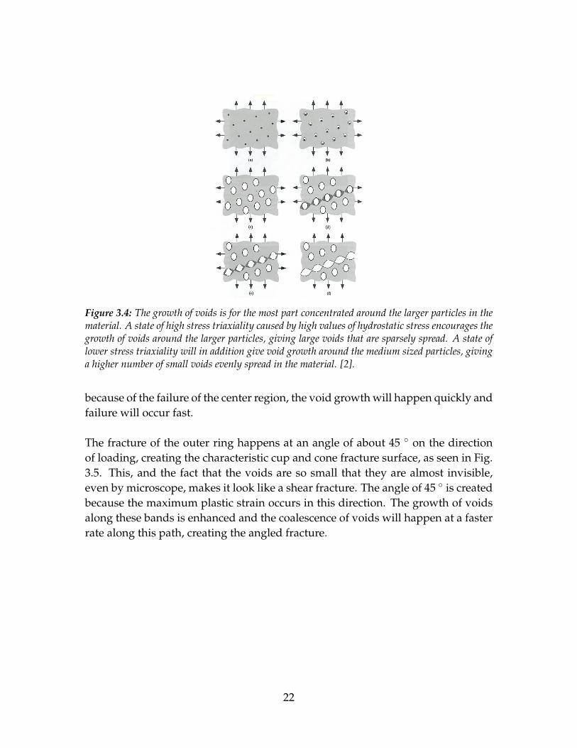
Figure 3.4: The growth of voids is for the most part concentrated around the larger particles in thematerial. A state of high stress triaxiality caused by high values of hydrostatic stress encourages thegrowth of voids around the larger particles, giving large voids that are sparsely spread. A state oflower stress triaxiality will in addition give void growth around the medium sized particles, givinga higher number of small voids evenly spread in the material. [2].

because of the failure of the center region, the void growth will happen quickly andfailure will occur fast.

The fracture of the outer ring happens at an angle of about 45 ◦ on the directionof loading, creating the characteristic cup and cone fracture surface, as seen in Fig.3.5. This, and the fact that the voids are so small that they are almost invisible,even by microscope, makes it look like a shear fracture. The angle of 45 ◦ is createdbecause the maximum plastic strain occurs in this direction. The growth of voidsalong these bands is enhanced and the coalescence of voids will happen at a fasterrate along this path, creating the angled fracture.

22

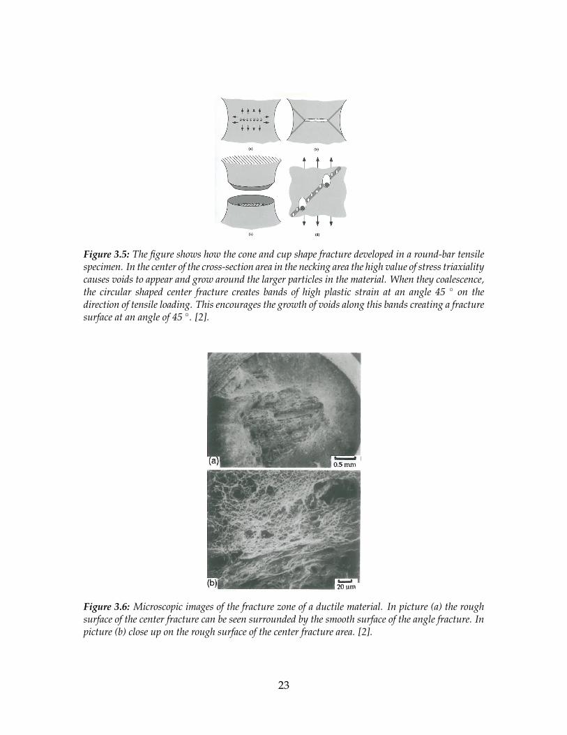
Figure 3.5: The figure shows how the cone and cup shape fracture developed in a round-bar tensilespecimen. In the center of the cross-section area in the necking area the high value of stress triaxialitycauses voids to appear and grow around the larger particles in the material. When they coalescence,the circular shaped center fracture creates bands of high plastic strain at an angle 45 ◦ on thedirection of tensile loading. This encourages the growth of voids along this bands creating a fracturesurface at an angle of 45 ◦. [2].

Figure 3.6: Microscopic images of the fracture zone of a ductile material. In picture (a) the roughsurface of the center fracture can be seen surrounded by the smooth surface of the angle fracture. Inpicture (b) close up on the rough surface of the center fracture area. [2].

23

3.2.3 Mathematic models for predicting the growth of voids andonset of fracture.

Several models have been made in order to describe the behavior of void growthleading to failure of the material. One is made by Rice and Tracey [21] and de-scribes the growth of one single void in an infinite solid subjected to remote prin-ciple stresses (σ1,σ2,σ3) and remote strain rates (ε1, ε2, ε3). The void is assumedto be spherical in its initial state, but deforms into an ellipsoidal shape. Rice andTracey concluded that the growth of one void representing the voids in the ma-terial can be approximated as the ratio of radial size of the assumed void to theinitial radius of the undeformed void.

This model has the weakness of not being able to account for the coalescence ofvoids as they grow ever larger, since only one void is present in the material model.The model is also unable to predict the failure of the material. A failure criterioncan be introduced by saying that the material is assumed to fail once a preset voidradius size has been reached.

Another model is presented by Gurson [12] and later modified by Tvergaard [22,23]. It assumes that the voids are homogeneously distributed in a continuous ma-terial. It differs from classical plastic theory by being dependent on the hydrostaticstress in the material in order to define the yield surface, and thereby introduces astrain-softening effect to the plastic material. The model assumes that the growthof voids results in a yield surface defined as a function of void volume, the equiva-lent stress, the hydrostatic stress and the flow stress in the matrix material, as seenin Eq. (3.6) ([2] pg. 229).

g(σe,σm, σ , VV) = 0 (3.6)

The model given by Gurson and Tvergaard assumes that the failure of the mate-rial occurs when the plastic strain causes a local instability in the form of localizedstrain bands. Because the voids are assumed to be a homogeneous part of a contin-uous material, the onset of local instability from necking of the void sidewalls cannot be predicted. Thomason ("Ductile fracture of metals" 1990) introduces a simplemodel to determined when this instability takes place. He assumes that in a planeloading state (ε3 = 0) the fracture due to local instability in the sidewalls between

24

voids (coalescence of voids) takes place when the stress in the section between thevoids σn reaches a critical value σn(c). If a is the length of a void in the direction ofσ1, b is the width of the void, and d is the distance between two voids (the thicknessof the side wall dividing two voids) then fracture is predicted to occur when

σn(c)0.5d

0.5(d + b)= σ1 (3.7)

All of these models are assumptions made in order to best predict the onset offracture due to coalescence of voids. In most material the fracture will occur dueto minimal increase in the nominal strain when the void volume fraction is overabout 10-15 % ([2] pg. 231)

25

Chapter 4

Fracture mechanic parameters

4.1 Introduction

In this chapter, different parameters that have an influence on the behavior of duc-tile materials, particularly when it comes to fracture, are presented. In a real struc-ture, the onset of damage can be expected to occur around weaknesses in the ma-terial, as explained in chapter 3. In a finite element based numerical analysis, thematerial are assumed to be homogeneous, and there is no weak part of the materialwhere the fracture can start to develop. To overcome this problem, it is commonto introduce some form of an initiation criterion, based on measurable values ofstress, strain or energy parameters. To be sure that the material behaves equallyin every direction, parameters that are independent on the coordinate system theyare calculated from must be used. This means that for a given state of e.g. stress,there will be equivalent scalar value of stress that is independent of the coordinatesystem that the stress components it are calculated from are defined in. This en-sures that the coordinate system used in the analysis does not influence the resultregarding fracture.

The term equivalent points to this ability to be independent of the directions, andalways giving the same result regardless of th coordinate system its componentsare calculated in. At the same time the equivalent value of a parameter does notdisplay the whole truth, and its value is in most cases somewhat smaller than themaximum of its components.

26

The following section gives an explanation of the most used parameters related tofracture initiation and development.

4.2 Stress parameters

4.2.1 the von Mises equivalent stress

The von Mises equivalent stress comes from the von Mises criterion which is a yield-ing criterion used when simulating yielding of isotropic ductile materials such asmetals, as explained in section 3.2. For anisotropic ductile yielding, the Hill yieldsurface criterion can be used. The von Mises criterion suggests that the yieldingof the material starts when the equivalent stress σe is equal to a critical value de-fined as the uniaxial yield stress σY ([2] page 66). The von Mises stress for principalstresses is defined as ([6] pg. 117)

σe =1√2

[(σ1 −σ2)

2 + (σ1 −σ3)2 + (σ2 −σ3)

2]1/2

, (σ1 > σ2 > σ3) (4.1)

and defined from general stress components

σe =1√2

[(σxx −σyy)

2 + (σyy −σzz)2 + (σzz −σxx)

2 + 6(τ2

xy + τ2yz + τ

2zx

)]1/2.

(4.2)

The σ1, σ2 and σ3 are the three principal stresses, σxx, σyy and σzz is the stressand τxy, τyz and τxz is the shear stress. σe is a scalar stress value representing aneffective stress occurring in the body. Equation (4.1) defines a cylindrical surfacein the space defined by the three principal stresses, around the hydrostatic axisdefined as σ1 = σ2 = σ3, see figure (4.1).

A material is assumed to change from purely elastic behavior into elasto-plasticbehavior when the equivalent stress exceeds a limit set as the yield stress σY.

27

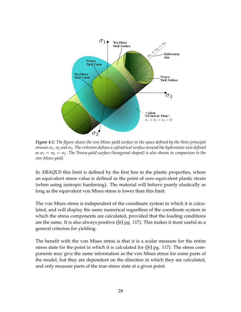
Figure 4.1: The figure shows the von Mises yield surface in the space defined by the three principalstressesσ1,σ2 andσ3. The criterion defines a cylindrical surface around the hydrostatic axis definedas σ1 = σ2 = σ3. The Tresca-yield surface (hexagonal shaped) is also shown in comparison to thevon Mises yield.

In ABAQUS this limit is defined by the first line in the plastic properties, wherean equivalent stress value is defined as the point of zero equivalent plastic strain(when using isotropic hardening). The material will behave purely elastically aslong as the equivalent von Mises stress is lower than this limit.

The von Mises stress is independent of the coordinate system in which it is calcu-lated, and will display the same numerical regardless of the coordinate system inwhich the stress components are calculated, provided that the loading conditionsare the same. It is also always positive ([6] pg. 117). This makes it most useful as ageneral criterion for yielding.

The benefit with the von Mises stress is that it is a scalar measure for the entirestress state for the point in which it is calculated for ([6] pg. 117). The stress com-ponents may give the same information as the von Mises stress for some parts ofthe model, but they are dependent on the direction in which they are calculated,and only measure parts of the true stress state at a given point.

28

4.2.2 Hydrostatic stress/Pressure stress

The hydrostatic stress σm is also known as the pressure stress. It is an averageof the three principle stresses in a body, and is often used as a parameter for thestress state of the material. The hydrostatic stress is defined as the stress that causesvolumetric changes to a volume of solid, and does not alter the shape of the volume(just resizing it). The shape is being influence by the deviatoric stress state, and thetotal stress state is the sum of the hydrostatic state and the deviatoric state ([6] pg.609). Hydrostatic stress is defined as [10]

σm = −p =13(σ1 +σ2 +σ3) (4.3)

p is the equivalent hydrostatic pressure, and is related to the hydrostatic stressσm as seen above. The negative sign in front of p comes from the definition ofthat compression is normally denoted as negative and tensile positive, but sincep is a measure for the pressure state of a volume it is defined as positive when incompression.

The hydrostatic stress is defined by the three principle stresses alone, it containsno form of shear deformation, since the principle stresses are defined by prin-ciple planes elimination the shear stresses. The hydrostatic stress is the stresscomponents that are responsible for changing the volume of a predefined vol-ume of a solid. From Eq. (4.4) it can been seen that the hydrostatic stress isσm = −p = σ´−σ .

In the space defined by the three principle stresses the hydrostatic stress is a vectorlying in the von Mises surface, parallel with the hydrostatic axis (σ1 = σ2 = σ3),starting in the deviatoric plane (π plane) as seen in Fig. 4.1.

Hydrostatic stress is greatly influencing the material behavior when voids are de-veloping and growing in materials exposed for ductile fracture, since the stress tri-axiality discussed below is dependent on the hydrostatic stress and the von Misesequivalent stress. In a localized necking zone, the equivalent stress may have aboutthe same value all over, but the center region of the volume is experiencing a higherhydrostatic pressure stress than the outer parts of the volume, and therefore it hasa higher value of stress triaxiality.

29

4.2.3 Deviatoric stress

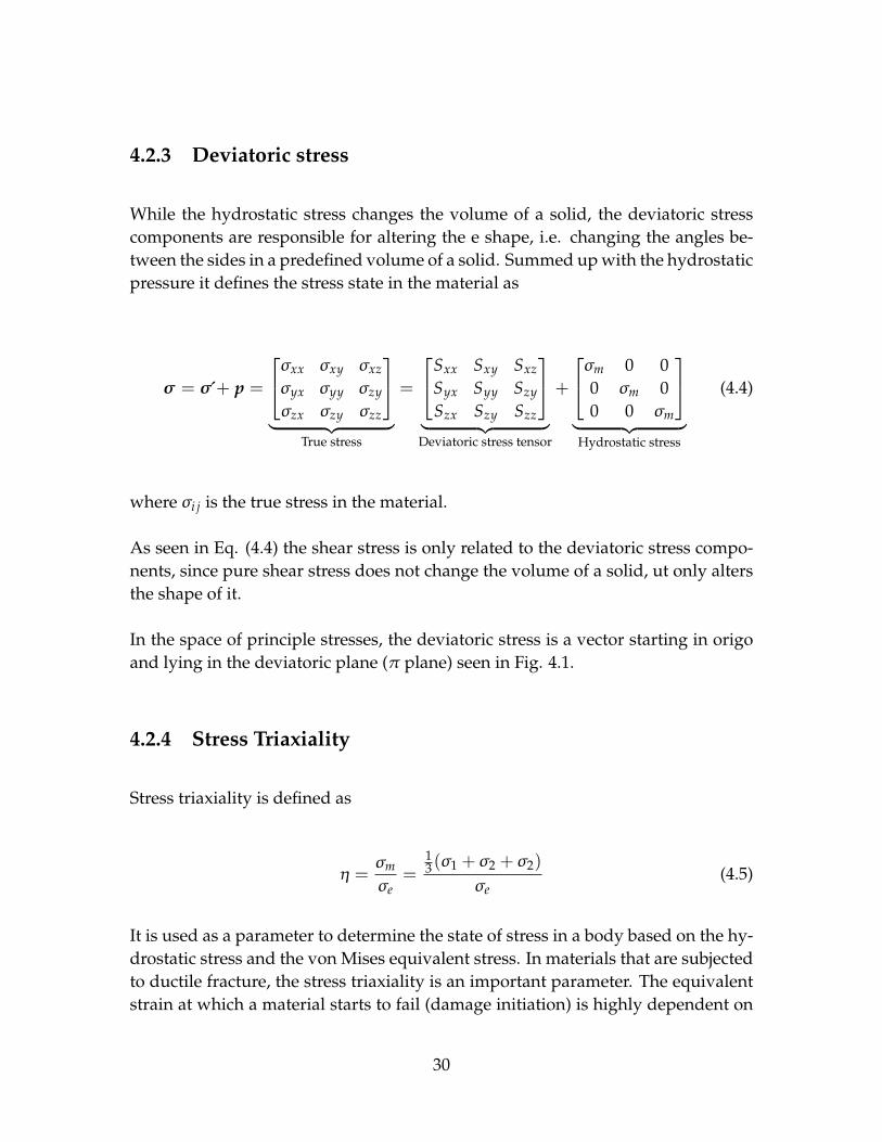
While the hydrostatic stress changes the volume of a solid, the deviatoric stresscomponents are responsible for altering the e shape, i.e. changing the angles be-tween the sides in a predefined volume of a solid. Summed up with the hydrostaticpressure it defines the stress state in the material as

σ = σ´+ p =

σxx σxy σxz

σyx σyy σzy

σzx σzy σzz

︸ ︷︷ ︸

True stress

=

Sxx Sxy Sxz

Syx Syy Szy

Szx Szy Szz

︸ ︷︷ ︸Deviatoric stress tensor

+

σm 0 00 σm 00 0 σm

︸ ︷︷ ︸Hydrostatic stress

(4.4)

where σi j is the true stress in the material.

As seen in Eq. (4.4) the shear stress is only related to the deviatoric stress compo-nents, since pure shear stress does not change the volume of a solid, ut only altersthe shape of it.

In the space of principle stresses, the deviatoric stress is a vector starting in origoand lying in the deviatoric plane (π plane) seen in Fig. 4.1.

4.2.4 Stress Triaxiality

Stress triaxiality is defined as

η =σm

σe=

13(σ1 +σ2 +σ2)

σe(4.5)

It is used as a parameter to determine the state of stress in a body based on the hy-drostatic stress and the von Mises equivalent stress. In materials that are subjectedto ductile fracture, the stress triaxiality is an important parameter. The equivalentstrain at which a material starts to fail (damage initiation) is highly dependent on

30

Figure 4.2: The figure shows the development of equivalent stress, stress triaxiality and hydrostaticstress for two elements in a tensile test simulation performed using the ABAQUS software package.The center element is experiencing higher hydrostatic stress than the element on the edge of the plateafter the initiation of necking, at the point of 5.5 sec. This increases the amount of stress triaxialityin the element.

the stress state of the material, hence the stress triaxiality.

In a fracture zone of a material, the equivalent stress may be about the same valueall over. Experiments have shown that ductile fracture due to growth and coales-cence of voids is initiated in the center of the volume. When a material is necking,a volume inside the necking zone is strained in tension in the direction of the mainprinciple stress σ1, and compressed in the two transverse directions because thethickness and width of the specimen is reduced by the necking phenomenon. Thiscreates a state of high hydrostatic stress leading to a higher state of triaxial stressin the volume. A volume which is located nearer the edge of the specimen will nothave the same amount of hydrostatic stress because the straining of this element ismore of a shape altering strain than a volume changing one.

The influence of the stress triaxiality on the behavior of a material in post neckingstate can be seen in Fig. 4.2. Two elements in a tensile test simulation performedwith the ABAQUS software package are compared. The center-element is locatedat the center of the plate, inside the necking area, and the edge-element is locatedat the edge of the model. Both elements are at the mid span of the model. Up to the

31

point of necking, the stress states of the two elements are equal, but after aroundsix seconds the hydrostatic pressure of the center element starts to rise. This causesthe hydrostatic pressure to increase. It can be seen that the von Mises stress in bothelements is similar. In this model, the center element will fail before the elementon the edge, because of the increasing value of the stress triaxiality caused by thehigh value of compression stress.

Studies have shown that the effect of stress triaxiality in a material is a parameterthat is not possible to avoid, and that the best way to cope with its effect is to beaware of it and try to use materials that can withstand its effects on the structure[5].

4.3 Strain parameters

4.3.1 Equivalent plastic strain

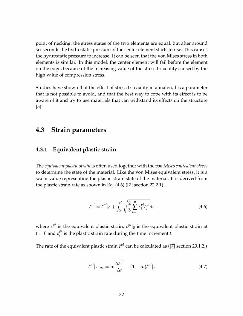
The equivalent plastic strain is often used together with the von Mises equivalent stressto determine the state of the material. Like the von Mises equivalent stress, it is ascalar value representing the plastic strain state of the material. It is derived fromthe plastic strain rate as shown in Eq. (4.6) ([7] section 22.2.1).

εpl = εpl|0 +∫ t

0

√23

n

∑i=1ε

pli ε

pli dt (4.6)

where εpl is the equivalent plastic strain, εpl|0 is the equivalent plastic strain att = 0 and εpl

i is the plastic strain rate during the time increment t.

The rate of the equivalent plastic strain ˙εpl can be calculated as ([7] section 20.1.2.)

˙εpl|t+∆t =ω∆εpl

∆t+ (1−ω) ˙εpl|t (4.7)

32

where ∆εpl is the change in equivalent plastic strain during the time increment ∆t.ω is a factor that dampens out high-frequency oscillations occurring in strain-rate-dependent materials.

Like the von Mises equivalent stress, the equivalent plastic strain is a simplificationof a more complex state in the material. The benefit of the equivalent plastic strainis that it is a simpler way to describe the strain state in the material than looking ateach strain component for themselves.

4.4 Other parameters related to yielding and fractureof ductile materials

4.4.1 Lode parameter and lode angle

For decades, the stress triaxiality has been the only parameter associated with frac-ture due to void growth and coalescence in ductile materials. Recently, it has beendiscovered that there is a second parameter involved in characterizing the stressstate of the material [4]. The lode parameter gives information of the state of stressin the material for a given von Mises equivalent stress by implying that the mainstress is caused by axial or shear stress components. The lode parameter is definedas ([14] pg. 18)

Lσ =2σ3 −σ1 −σ2

σ1 −σ2, Lσ ∈< −1, 0 > (4.8)

Lσ = −√

3tanθ (4.9)

The lode parameter is always in the range of −1 to 0, representing uniaxial stressstate and pure shear stress state respectively. (uniaxial stress state: σ1 6= 0,σ2 =

σ3 = 0, pure shear stress state: σ3 = 12(σ1 +σ2) giving 1

2(σ1 −σ2,σ2 −σ1, 0))

In [3], Bai and Wierzbicki presents a new plasticity model taking into account theinfluence of both the hydrostatic stress state and the lode parameter for the mate-rial stress state. They define the parameter known as the lode angle to be the angle

33

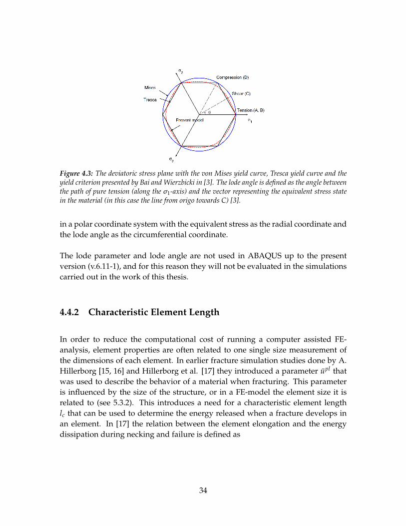
Figure 4.3: The deviatoric stress plane with the von Mises yield curve, Tresca yield curve and theyield criterion presented by Bai and Wierzbicki in [3]. The lode angle is defined as the angle betweenthe path of pure tension (along the σ1-axis) and the vector representing the equivalent stress statein the material (in this case the line from origo towards C) [3].

in a polar coordinate system with the equivalent stress as the radial coordinate andthe lode angle as the circumferential coordinate.

The lode parameter and lode angle are not used in ABAQUS up to the presentversion (v.6.11-1), and for this reason they will not be evaluated in the simulationscarried out in the work of this thesis.

4.4.2 Characteristic Element Length

In order to reduce the computational cost of running a computer assisted FE-analysis, element properties are often related to one single size measurement ofthe dimensions of each element. In earlier fracture simulation studies done by A.Hillerborg [15, 16] and Hillerborg et al. [17] they introduced a parameter upl thatwas used to describe the behavior of a material when fracturing. This parameteris influenced by the size of the structure, or in a FE-model the element size it isrelated to (see 5.3.2). This introduces a need for a characteristic element lengthlc that can be used to determine the energy released when a fracture develops inan element. In [17] the relation between the element elongation and the energydissipation during necking and failure is defined as

34

G f =∫ upl

f

0σdupl (4.10)

G f is the energy dissipated per unit area by the fracturing of the material, and can

be considered a material constant [16], and uplf is the total elongation of the element

from damage initiation to failure.

From the work of A. Hillerborg the definition of the characteristic element length isthe dimension of the element in the direction of the elongation. Since this work wascarried out on simple bar elements with only two nodes, this must be generalizedsome more. ABAQUS has adopted much of the theory presented by A. Hillerborgel. al. [17] and presents a definition that is generalized to apply for all types ofelements:

The definition of the characteristic length depends on the element ge-ometry and formulation: it is a typical length of a line across an ele-ment for a first-order element; it is half of the same typical length for asecond-order element. For beams and trusses it is a characteristic lengthalong the element axis. For membranes and shells it is a characteristiclength in the reference surface. For axisymmetric elements it is a char-acteristic length in the r− z plane only. For cohesive element it is equalto the constitutive thickness ([7] section 20.2.3.).

An elements can have different side lengths in the different directions. It is rec-ommended to use elements with side lengths as equal as possible, thus giving theelements the same properties in every direction when it comes to fracture modu-lating. This reduces, but does not eliminate, the dependency of the element mesh.

The characteristic element length presented here can be related to the strain ref-erence length used by Ehlers and Varsta in [11], and that is descussed in section5.2.

35

Figure 4.4: a) The path of a crack through a plate modeled with shell elements. b) The path of thecrack through one of the elements, with the normal vector n defining the direction of the elongationof the crack [20].

A model for calculation the element length for shell elements

In recent times there have been presented models that try to eliminate the meshdependency altogether. An article written by J. Oliver [20] presents a method forshell elements that uses the dissipated fracture energy, assumed to be a materialparameter and therefore constant throughout the material, and relates it to a crackangle in order to find a characteristic element length.

In a plate modeled by quadratic shell elements, a crack will take a random paththrough the plate and randomly through the elements making up the plate. Such arandom path can be seen going through the element in Fig. 4.4. For each element,the energy that must be dissipated is a function of the elements base functions, theangle of the crack path through the element and which edges of the element thecrack path goes through. Using these parameters a characteristic length for theelement can be calculated as

lc =

(∂φ(ξ j, η j)

∂x

)−1

=

(ne

∑i=1

[∂Ni(xi j, η j)

∂xcosθ j +

∂Ni(ξ j, η j)

∂ysinθ j

]φi

)−1

(4.11)

36

Here, Ni is the base functions for the element j node i, defined in the coordinatesystem (ξ , η) with origo of the coordinate system in the middle of the shell ele-ment. x is the x-axis of the coordinate system defined by having the y parallel tothe crack going through the element, and the the x-axis in the direction of the elon-gation of the crack. θ j is the angle of rotation between the two coordinate systemsfor element j. φi is either zero or one depending on which side of the crack thenode i is located, see Fig. 4.4.

This method can be used to remove the mesh dependency of the fracture criterionin a finite element analysis. But the computational resources needed to calculatethe characteristic element length for each element is high, and software programslike ABAQUS uses less demanding definitions that will give sufficiently preciseresults of equivalent element lengths.

37

Chapter 5

Fracture models in the finite elementmethod

5.1 Introduction

In the finite element method, the structure has to be simplified into a finite num-bers of elements that have more or less the same properties all over. The idealapproach is to have uniform elements all over, of the same size and with the sameproperties regarding stiffness, mass and other material related properties. The be-havior of the structure is dependent on the inputted data regarding how each ele-ment is supposed to respond to load cases and straining. For the elastic behavior ofthe element the deformation is small and evenly spread out through the structure.For the plastic behavior the same applies as long as the straining of the material issmaller than the combination of strain and stress values that will bring the materialup to its point of ultimate strength.

In the FE-method, the model’s behavior are independent of the element size usedin the mesh of the model, within certain limits. Two models shearing the samematerial input will behave more or less in the same way for a specific load case,even if the element sizes used are different. Some effects may arise due to poorlychosen mesh, where some element may be deformed in a manner that produceseffects that are not realistic. This includes shear locking in shell elements, majordistortion of elements due to unfortunate deformation of elements or the solution

38

may not converge because there are too few elements being used.

As long as the mesh is capable of representing the structure under the loading con-ditions applied, the size of the element in the mesh should not influence the resultup to the point of ultimate loading. For ductile materials, the effect of passing thepoint of ultimate strength is explained in section 3.1. In a FE-model, whats happensis that the continued elongation of the model is being concentrated into strainingof a few elements, representing the instability zone. During this deformation, theelement size is crucial. Since the elongation is produced through straining of per-haps as little as one element, the properties of this element alone now govern thebehavior of the whole model.

Stress

Strain

ds1

s0 s1

Force

Elongation

de

e0 e1

coarse mesh

fine mesh

ds2

s2

Δl

l0 l1

dεcoarse

dεfine

ε0 ε1ε2

Figure 5.1: The figure illustrates the relationship between the true strain in the element of a FE-analysis, and the global elongation of the model. For models containing smaller elements, the truestrain increases by a higher value than for a corresponding model with larger elements. This makesthe fine meshed model behave more soft than the model with larger elements in a post-ultimatestrength state.

If the same model is meshed using two different element sizes, but the mate-rial properties are kept the same, the global response after the point of ultimatestrength for the coarser meshed model will be stiffer than for the finer meshedmodel. This is a result of the effect of the global elongation being dependent ontrue stress/true strain relationship in only one element, as the elongation contin-ues beyond the point of ultimate strength. At the point of ultimate strength theelongation l0 of the model is

39

l0 = lenelem ε (5.1)

where le is the element length, nelem is the numbers of elements and ε is the strainin the elements. The elongation of the model is spread out evenly as strain in theelements. If both models are supposed to elongate the same amount ∆l from thepoint of ultimate strength (Fig. 5.1), the true strain in the element being strained inthe fine meshed model must be

∆l = δε f ine lef ine = (ε2 −ε0)le

f ine (5.2)

where ε0 is the true strain at the point of ultimate strength and ε2 is the true strainat the point of elongation l1 for the fine meshed model. Le

f ine is the element length.The same relationship for the coarser meshed model will be

∆l = δεcoarse lecoarse = (ε1 −ε0)le

coarse (5.3)

where ε1 is the true strain in the element for the coarse meshed model when elon-gated to l1.

∆l are equal in Eq. (5.3) and Eq. (5.3), so substituting the two equation into eachother yield

δε f ine lef ine = δεcoarse le

coarse (5.4)

Since lecoarse is larger than le

f ine, then δε f ine must be larger than δεcoarse, henceε2 > ε1.

The coarse meshed model has a higher stiffness (the slope of the true stress/truestrain curve lies higher) while elongating from l0 to l1 than the fine meshed modeldoes. This makes the finer mesh model act more softly, giving a steeper drop inthe force-displacement curve after the point of ultimate strength.

Since the post-ultimate strength behavior is dependent on the mesh, the plastic

40

properties, calculated as the engineeering strain cannot be used directly to modelthe material during this part of deformation. This calls for the introduction offracture models, since this behavior is due to ductile fracturing of the material.Two different approaches to model the post-ultimate strength behavior follows inthis chapter.

5.2 A fracture model using the true stress/true strainrelationship

5.2.1 Introduction

In the scientific journal Thin-Walled Structures Sören Ehlers and Petri Varsta fromthe Helsinki University of Technology present a method for modeling the local in-stability up to the point of fracture, causing necking in a material under tensileloading by tuning the plastic properties for the material in the FE-model [11]. Theidea is to get around the limit of validity for the true stress/true strain relationshipobtained from the engineering strain measured in a material test, as explained inSection 2.1. The data used for the stress and strain relationship is related to an ele-ment’s length, called the strain reference length, and is obtained from tensile testsof the material where the strain is optically measured at the surface of the mate-rial in the necking zone. The related stress is obtained independently of the strain,from calculating the cross-section area by measuring the contraction of the materialin the width and thickness of the tensile specimen, and dividing the load on thiscalculated cross-section area. The tensile tests are done on three flat-bar dog-boneshaped tensile specimens with different length to width rations, The thickness was5.87 mm for two of the specimens (referred to as 6 mm) and the third being 4.04 mmthick (4 mm). The surface strain in the necking zone of the material is measuredusing stereoscopic cameras that could trace the relative movements of a stochasticpattern of black and white pixels painted on the surface of the specimen.

When a relationship for the stress and strain for the material was established fordifferent strain reference lengths, this data was used as input for the material prop-erties when simulating the tensile test using the FE-analysis program LS-DYNA.The element size used in the FE-analysis was the same as the strain reference length

41

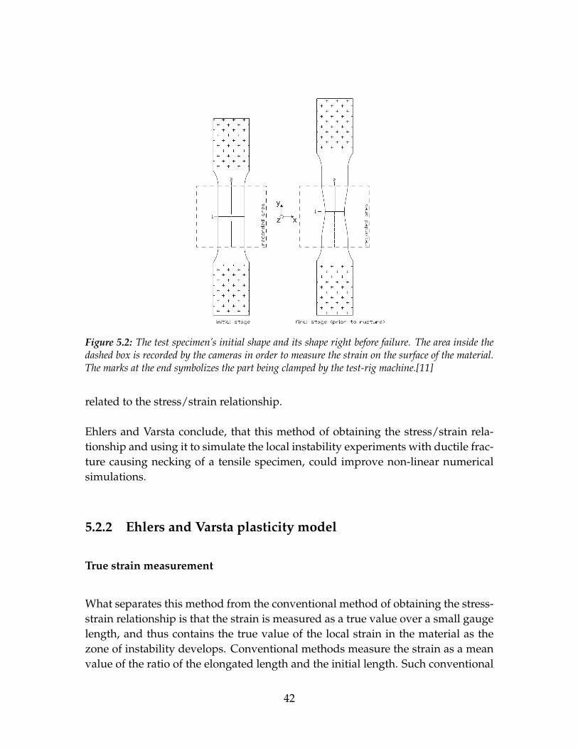
Figure 5.2: The test specimen’s initial shape and its shape right before failure. The area inside thedashed box is recorded by the cameras in order to measure the strain on the surface of the material.The marks at the end symbolizes the part being clamped by the test-rig machine.[11]

related to the stress/strain relationship.

Ehlers and Varsta conclude, that this method of obtaining the stress/strain rela-tionship and using it to simulate the local instability experiments with ductile frac-ture causing necking of a tensile specimen, could improve non-linear numericalsimulations.

5.2.2 Ehlers and Varsta plasticity model

True strain measurement

What separates this method from the conventional method of obtaining the stress-strain relationship is that the strain is measured as a true value over a small gaugelength, and thus contains the true value of the local strain in the material as thezone of instability develops. Conventional methods measure the strain as a meanvalue of the ratio of the elongated length and the initial length. Such conventional

42

methods of calculating the strain do not isolate the effect that the local instabil-ity has on the elongation, but evens its effects out over the whole specimen. Thismakes the stress/strain relationship obtained from measuring the global elonga-tion not valid after the point of ultimate strength, since the straining of the speci-men after this point is concentrated in the necking zone, while the material outsideof this zone recovers elastically ([14] pg. 12).

Ehlers and Varsta used cameras taking stereo pictures of the surface of the neck-ing zone of the tensile specimen when the load was increased from zero throughultimate strength and to fracture. These cameras were able to trace facets of pixelspainted on the surface of the specimen, and the strain was measured as the relativeelongation of a distance between two facets. The initial distance between the facetswas uses as the gauge length and referred to as the strain reference length.

The strain reference length was used to relate the obtained stress/strain relation-ship to an element size in the FE-model when the data was used in a FE-analysis.As for a FE-model where the smallest length which the strain in the model can bemeasured over are the distance between the nodes (i.e. the element length for firstorder elements and half the element length for second order elements), the smallestdistance the strain could be measured over was the strain reference length deter-mined by the facet size.

The facet sizes used ranged from 10x10 pixels to 50x50 pixels, giving a strain ref-erence length ranging from 0.88 mm to 4.4 mm. A total of seven different strainreference lengths were used to measure the true strain for seven different meshsizes in the following FE-analysis. The true strain was measured as

εtrue = lnl + δl

l(5.5)

where l is the strain reference length and δl is the change in the length of l.

Determination of true stress

The true stress related to the true strain measurement explained above, was calcu-lated on the basis of the transverse displacement of the edges in the necking zone

43

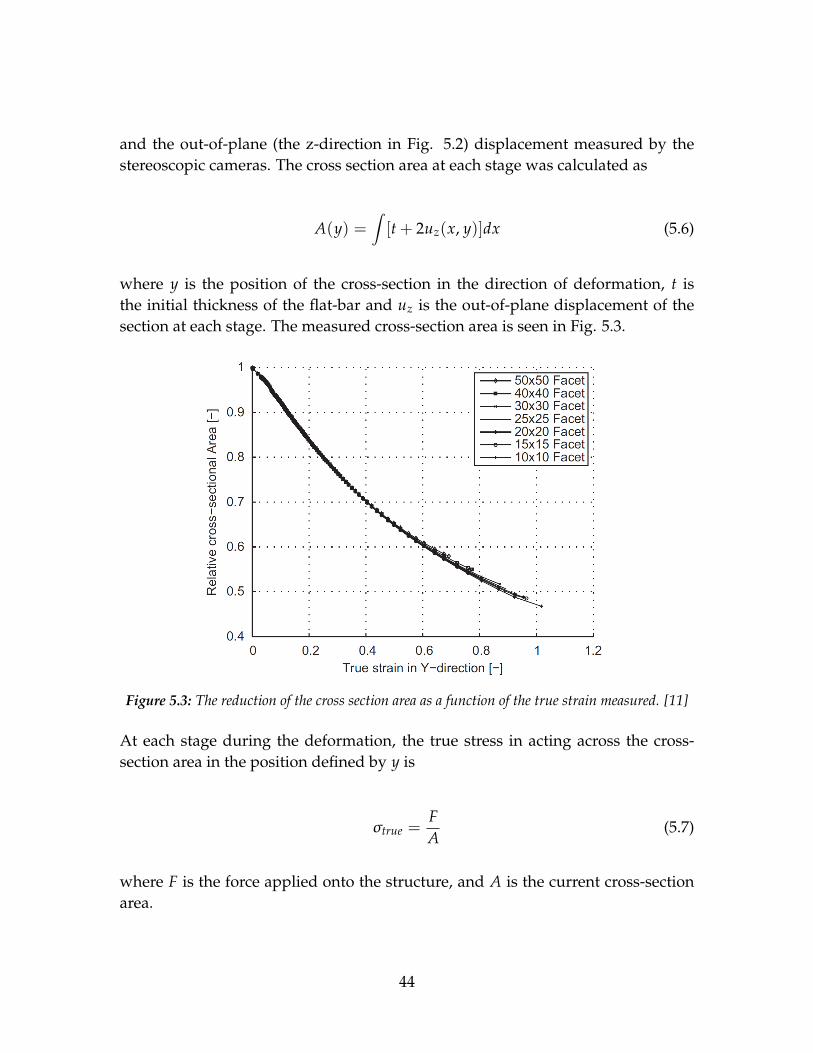
and the out-of-plane (the z-direction in Fig. 5.2) displacement measured by thestereoscopic cameras. The cross section area at each stage was calculated as

A(y) =∫[t + 2uz(x, y)]dx (5.6)

where y is the position of the cross-section in the direction of deformation, t isthe initial thickness of the flat-bar and uz is the out-of-plane displacement of thesection at each stage. The measured cross-section area is seen in Fig. 5.3.

Figure 5.3: The reduction of the cross section area as a function of the true strain measured. [11]

At each stage during the deformation, the true stress in acting across the cross-section area in the position defined by y is

σtrue =FA

(5.7)

where F is the force applied onto the structure, and A is the current cross-sectionarea.

44

Table 5.1: The strain reference length, the corresponding facet size used when optically measuringthe local strain at the surface of the material of the tensile specimen, and the element size used whenreproducing the results in LS-DYNA [11].

Strain reference length Facet size Element side length[mm] [pixes] [mm]0.88 10x10 0.881.32 15x15 1.321.76 20x20 1.762.2 25x25 2.22.64 30x30 2.643.52 40x40 3.524.4 50x50 4.4

Implementation of the true stress-true strain relationship into the FE-model

The true stress/true strain relationships that were measured using a different gaugelength on the different tensile test specimens were used to recreate the tests in theFE-analysis software LS-DYNA. The element type used were four nodded quadri-lateral Belytschko-Lin-Tsay shell elements, and the analysis was performed usingthe explicit time integration solver in LS-DYNA. Each of the three different tensilespecimens was meshed with seven different element sizes (see table 5.1)

The stress and strain relationship obtained for the corresponding tensile specimenmeasured using a strain reference length equal to the element side length was in-putted as the plastic properties for the material. Then the tensile experiments werereproduced using the FE-method and LS-DYNA. The force-displacement curvefrom the finite element analysis was compared against the force-displacement curverecorded during the tensile testing of the specimens. They show good agreementbetween the recorded results and the results from the finite element method.

The method of obtaining the stress and strain relationship proposed by Ehlers andVarsta in [11] does not include any fracture criterion, and the FE-models behavioris only controlled through its plastic material properties.

45

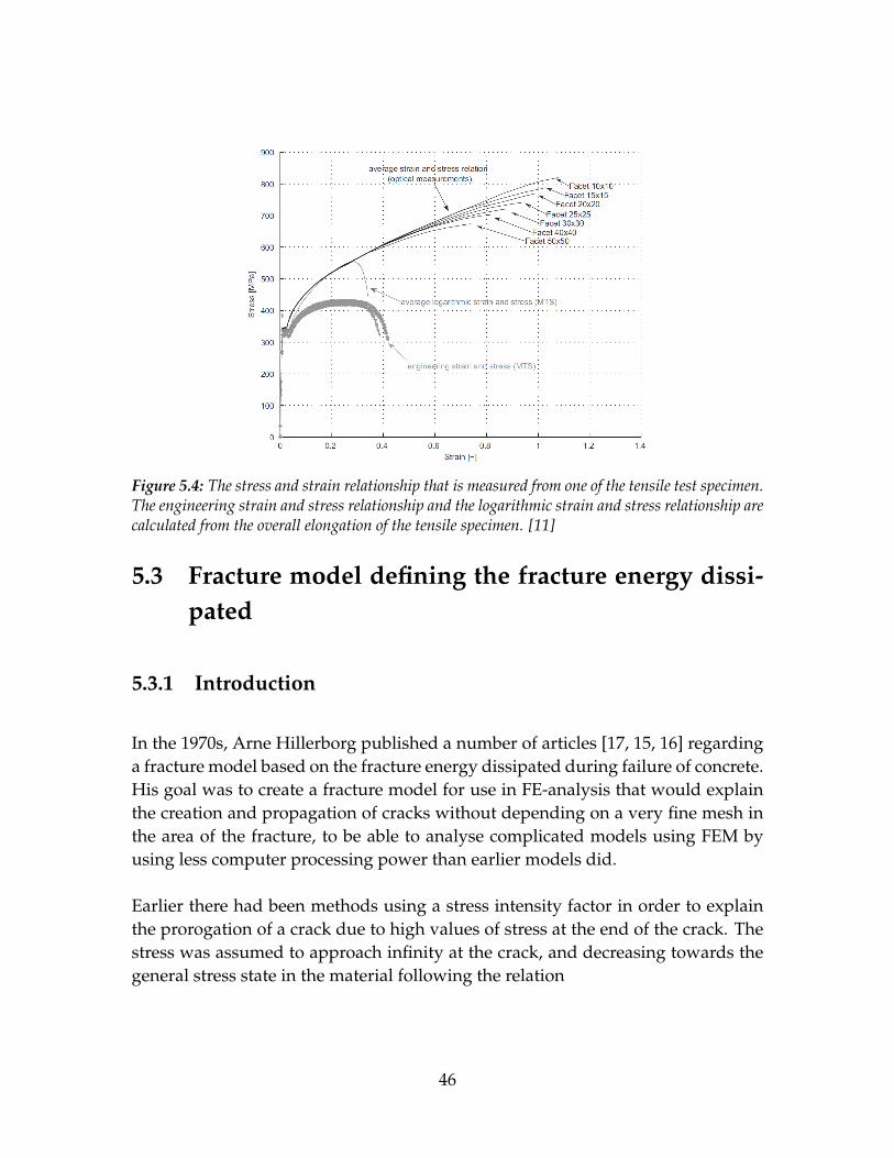
Figure 5.4: The stress and strain relationship that is measured from one of the tensile test specimen.The engineering strain and stress relationship and the logarithmic strain and stress relationship arecalculated from the overall elongation of the tensile specimen. [11]

5.3 Fracture model defining the fracture energy dissi-pated

5.3.1 Introduction

In the 1970s, Arne Hillerborg published a number of articles [17, 15, 16] regardinga fracture model based on the fracture energy dissipated during failure of concrete.His goal was to create a fracture model for use in FE-analysis that would explainthe creation and propagation of cracks without depending on a very fine mesh inthe area of the fracture, to be able to analyse complicated models using FEM byusing less computer processing power than earlier models did.

Earlier there had been methods using a stress intensity factor in order to explainthe prorogation of a crack due to high values of stress at the end of the crack. Thestress was assumed to approach infinity at the crack, and decreasing towards thegeneral stress state in the material following the relation

46

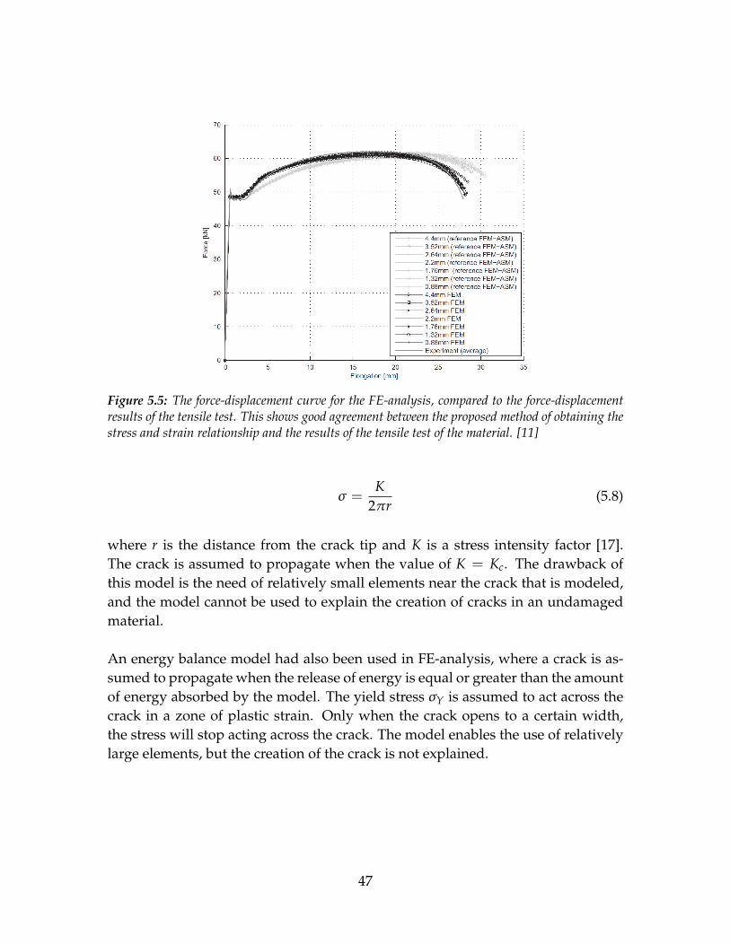
Figure 5.5: The force-displacement curve for the FE-analysis, compared to the force-displacementresults of the tensile test. This shows good agreement between the proposed method of obtaining thestress and strain relationship and the results of the tensile test of the material. [11]

σ =K

2πr(5.8)

where r is the distance from the crack tip and K is a stress intensity factor [17].The crack is assumed to propagate when the value of K = Kc. The drawback ofthis model is the need of relatively small elements near the crack that is modeled,and the model cannot be used to explain the creation of cracks in an undamagedmaterial.

An energy balance model had also been used in FE-analysis, where a crack is as-sumed to propagate when the release of energy is equal or greater than the amountof energy absorbed by the model. The yield stress σY is assumed to act across thecrack in a zone of plastic strain. Only when the crack opens to a certain width,the stress will stop acting across the crack. The model enables the use of relativelylarge elements, but the creation of the crack is not explained.

47

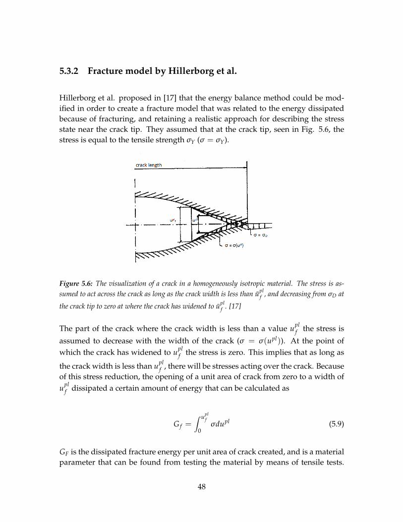
5.3.2 Fracture model by Hillerborg et al.

Hillerborg et al. proposed in [17] that the energy balance method could be mod-ified in order to create a fracture model that was related to the energy dissipatedbecause of fracturing, and retaining a realistic approach for describing the stressstate near the crack tip. They assumed that at the crack tip, seen in Fig. 5.6, thestress is equal to the tensile strength σY (σ = σY).

Figure 5.6: The visualization of a crack in a homogeneously isotropic material. The stress is as-sumed to act across the crack as long as the crack width is less than upl

f , and decreasing from σD at

the crack tip to zero at where the crack has widened to uplf . [17]

The part of the crack where the crack width is less than a value uplf the stress is

assumed to decrease with the width of the crack (σ = σ(upl)). At the point ofwhich the crack has widened to upl

f the stress is zero. This implies that as long as

the crack width is less than uplf , there will be stresses acting over the crack. Because

of this stress reduction, the opening of a unit area of crack from zero to a width ofupl

f dissipated a certain amount of energy that can be calculated as

G f =∫ upl

f

0σdupl (5.9)

GF is the dissipated fracture energy per unit area of crack created, and is a materialparameter that can be found from testing the material by means of tensile tests.

48

The energy dissipated per unit area crack is the area beneath the σ − ε-curve, andthe total energy dissipated inside the fracture zone is the area beneath the σ − upl-curve [16].

Figure 5.7: As the crack propagates, the stress will decrease as the width of the crack increases. Theenergy dissipated in the fracture zone by fracture is equal to the area beneath the σ − upl-curve.[17]

The shape of the curve in Fig. 5.7 determines the behavior of the material if itis loaded beyond the ultimate strength of the material. Different shaped σ −upl-curves may give the same value of G f , and therefore will dissipate the sameamount of energy due to fracturing, but they will behave differently because of thedifference in shape.

An advantage with to this model is that it is a general model that can be used topredict the failure of materials subjected to different kinds of loadings. It can alsopredict the creation of cracks in an element from the value of true strain or truestress in the element. The onset of damage is then said to be when the true strainreaches a critical value ε = εD or when the true stress is σ = σD. Often, the equiv-alent stress and strain values are used as initiation criterion because they measurethe strain and stress independently of the directions of the stress and strain com-ponents, see 4.2.1 and 4.3.1. The model also well adapted to be used in numericalcalculations, because the stress values are finite, and stress, deformation and dissi-pated energy are logically related.

When using the model proposed by Hillerborg et al., it must be clear that the modellaws does not apply to the structure after the initiation of failure. The model lawstates that two specimens with the same material, geometry and loading, but withdifferent size will behave equally by obtaining the same value of stress and strain ata corresponding point. If this is done using FEM and the fracture model proposedby Hillerborg et al., inputting the same data regarding σ and upl, the stress values

49

will be the same at corresponding point, but the value of upl will be proportionalwith the size of the specimen [15]. Said differently, the σ-upl-curve for a specimenmust be in relation to its size. If data developed for testing a small specimen isapplied in order to model fracture of a larger specimen, the larger specimen willfail at a lower value of strain ε than it should. (Both models should fail at the sameglobal strain value ε f , but with different values of elongation after the point ofultimate strength upl).

50

Chapter 6

Explicit dynamic analysis in FEM

6.1 Introduction

One choice that has to made when planning an analysis is which method shouldbe used to solve the problem numerically. In dynamic analysis, the explicit time in-tegration is favorable when solving problems containing high speed deformationswithin a short amount of time, because the method can calculate a high numberof incremental points close together in time, at a low computational cost. It ispreferred in cases where contact definitions between different part of a structuremodel is present [7]. The element size and the time used to run an explicit analysisare directly linked together through the critical time increment size ∆tcr, as definedin Section 6.3.2.

6.2 Dynamic analysis using direct integration meth-ods

When performing a FE-analysis there are many different methods offered to per-form dynamic analysis, each of them with advantages and disadvantages depend-ing on the problem you are trying to solve. One method that is often used fordynamic nonlinear analysis is the "explicit dynamic analysis method". For linear

51

dynamic analysis, it will in most cases be more effective to use analysis methodsbased on modal methods. They depend on calculating the eigenvalues of the sys-tem and then calculating the response of the model using these eigenvalues. Thecalculations performed in order to find the eigenvalue are costly, particularly sincethe number of eigenvalues that is needed for complicated structures is not knownbefore starting the analysis. The explicit dynamic analysis method uses direct-integration and integrates the global equation of motion through time. For linearanalysis this is not very effective, but for non-linear analysis, as collision eventsoften are, this direct-integration method is often more effective.

Direct integration is used to calculate the response history step-by-step in time.Each data point is calculated as a time increment ∆t after the previous calculations.For non-linear problem the equation of motion can be generalized as ([6] pg. 407)

[M]{u}n + [C]{u}n + {Rint}n = {Rext}n (6.1)

where [M] is the mass matrix of the system, [C] is the systems dampening matrix,{Rint} is the internal load vector and {Rext} is the external load vector. The equa-tion is calculated at the time increment n. The time factor is discretized using afinite difference approximation of the time derivatives. This can be done in manyways, but for application to dynamic collision events, the explicit time integrationis best suited.

6.3 Explicit analysis

In the explicit analysis, the displacement and the velocity at the beginning of eachincrement are known. This means that the global mass and stiffness matrix neednot be formed and inverted for each increment, saving much computational work.The size of the time increments however, have to be smaller than a critical timeincrement ∆tcr, see Section 6.3.2. This makes the method conditionally stable, andthe increments must be kept small enough to preserve the stability of the result.Since the incremental steps are small, the incremental result will never greatly de-viate from the exact solution, and any inaccuracy will most likely be correctedwhen calculating the next increment. Because of this there is often no need to con-

52

trol the accuracy as with the implicit method.

The stability of the method is related to the time it takes for a stress wave to movethrough an element. If the element is relatively small, or the wave is movingthrough the element at a high speed, the time increment must be small. Usuallythe increment must be smaller than the time it take a stress wave to get cross anelement, traveling the distance between to nodes. This makes the method good foranalysis where the total analyzing time is only a few orders of magnitude largerthan the stability limit. But also for some quasi-static processes where the use ofmass scaling is appropriate, which reduce the wave speed and therefore increasesthe length of the critical time increment in the analysis.

The explicit procedure is well suited for high-speed dynamic events, and slowerquasi-static analysis. In the case of high speed events, the small increments meanthat more detailed calculations are made and large deformation occurring over ashort time can be captured. For quasi-static analysis, the deformation is assumedto be to slow too cause dynamic response in the structure. The dynamic effect canbe neglected. The treatment of contact is also simplified, making it a good choicefor dynamic or quasi-static analysis containing contact between surfaces. The totaltime needed to run the analysis is linearly dependent on the size of the model andthe total time simulated, assumed that the mesh size is kept constant. A increaseof any of the two factors, will result in an equal increase in calculation time.

The explicit method is preferred before the implicit method because of the abilityto convert the mass matrix to a diagonal matrix, often referred to as lumped mass.This reduces the number of calculation needed for each time increment with up to4000 times for a three dimensional FE-analysis [6]. Also the amount of data storageneeded for each increment calculation is much smaller for the explicit method.

6.3.1 Central Difference Method

The explicit analysis method makes use of the central difference method to calcu-late the state of the next increment. The equilibrium equations are satisfied at thebeginning of each increment (ti). The acceleration at ti is used to find the veloc-ity at ti+ 1

2and the displacement at ti+1. Each calculation is relatively inexpensive,

and is done using "lumped" element mass matrices. The velocity (uNi+ 1

2) and the

53

displacement (uNi+1) is calculated as

uNi+ 1

2= uN

i− 12+

∆ti+1 + ∆ti

2uN

i

uNi+1 = uN

i + ∆ti+1uNi+ 1

2

(6.2)

where uN is a degree of freedom, and the subscript i is the increment number inthe analysis.

The efficiency of the procedure comes from the use of lumped stiffness matrices,which are diagonal. This makes it easier to calculate the acceleration at the begin-ning of each increment (Equ. (6.3), as the matrices are easy to invert and the vectormultiplication only demands one operation for each degree of freedom. The accel-eration is the calculated as

uNi = ([M]NJ)−1({Rext}J

i − {Rint}J

i ) (6.3)

where [M]NJ is the mass matrix, {Rext}Ji is the applied load vector and {Rint}J

i isthe internal force vector. The internal force vector is assembled with contributionsfrom individual elements in such a way that a global stiffness matrix is not needed.

6.3.2 Stability

The stability of the procedure is dependent on the highest frequency of the system.Equation (6.4a) shows the limit for a system with and without damping in thesystem, respectively.

∆t ≤ 2ωmax

(√1 +ξ2

max −ξmax

)(6.4a)

∆t ≤ 2ωmax

(6.4b)

54

Hereωmax is the maximum natural frequency, andξmax it the corresponding damp-ening ratio.

In ABAQUS, a small amount of dampening in the form of bulk viscosity is intro-duced to the system in order to control the high frequency oscillations that canoccur during an analysis. This effect is by default applied as a linear effect, but forsolid continuum elements it can also be a quadratic effect that is used in compres-sion state in order to prevent elements experiencing high velocity gradients whencollapsing, and the volume is suddenly reduced to zero.

6.3.3 Estimation of the stable time increment size

The size of the stable time increment ∆t is often estimated as being smaller than acritical time increment size ∆tc [6], that is

∆t ≤ ∆tc =lemincd

(6.5)

where Lmin is the smallest element dimension on the model, and cd is the speed ofsound in the material [6] over the element. cd is defined in equation (6.6). This isjust an estimated value of the maximum stable time increment. In most cases, it iswise to use a shorter time increment for the analysis. For two-dimensional modelsABAQUS uses a reduction factor between 1√

2and 1, and for three-dimensional

models 1√3

and 1. The speed of which the stress wave travels through a material isdependent on the Young-modulus E and the density ρ of the material.

cd =

√Eρ

(6.6)

From this it is clear that the critical time increment is increase if the material issofter (low Young-modulus) or has a high density. This can be used to manipulatethe time needed to run the explicit analysis on a computer.

55

6.3.4 Time reduction

The time spent on performing an explicit analysis is dependent on the size of theelement, the number of elements used and the time period being simulated. Fora model with a given mesh size, the time period simulated is the decisive factor.To reduce the time it take to run the analysis, there are some tricks that can beapplied. It is possible to speed up the simulation as compared to the time takenfor the actual event. Speeding it up too much may however introduce unwantedkinetic effects in the form of increased inertia forces that may change the outcomeof the simulation, or some rate dependent parameters may be triggered due to thehigher rate of change in the structure. If there are rate dependent parameters inuse, speeding up the simulation is not recommended because the rate of change isincreased, and it may change the result without the user being aware of it.

Another way to save time is to use mass scaling, artificially increasing the densityof the material ρ. This reduces the time period simulated as compared to the timetaken for wave propagation through an element, in effect increasing the value of∆tcr, making the simulation run faster. Rate dependent parameters will not beinfluenced by changing the density, but it has the same effect concerning inertiaeffects as speeding up the simulation.

A model with overall large elements, but with sections with smaller elements, willrun slowly because the time increment length is set by the size of the smallestelement in the model. If the number of small elements is significant smaller thanthe number of large element, a mixed time integration method can be applied. InABAQUS, this method sets different time incremental length for different sizedelements, meaning that the large elements are analysed by using fewer incrementsthan the smaller elements. The same central-difference integration rule as shown insection 6.3.1 is used, but different lengths of time increments are used for differentsets of nodes in the model.

6.3.5 Energy monitoring

In an explicit dynamic analysis, the energy in the model is important to monitor.The total energy in the model should be close to constant, and the artificial energiesshould be negligibly small compared to "real" energies as strain energy and kinetic

56

energy. For quasi-static analysis, the amount of kinetic energy should not exceeda certain fraction of the strain energy. For cases involving contact or constraints, itis wise to monitor the energy dissipated by constraint penalty and contact penalty.They should be close to zero in all cases. [7]

6.4 Single versus double precision

In the field of computer science, the terme single and double precision refer to thenumber of significant numbers used to store the computational data during a com-puter assisted FE-analysis [1]. For most cases single precision is sufficient to cal-culate the correct solution. This is not necessarily the case when using an explicitdynamic method. Since the time increments may become very small, the nodaldisplacement during a time increment may become so small that single precisionaccuracy does not calculate it precisely enough. The solution becomes affected byround-off errors that may propagate. Double precision is often recommended ifthe nodal displacement is anticipated to become to small, or if the numbers of timeincrements needed exceed a limit of 300 000 increments [7].

Running an analysis using double precision makes the round-off errors less likelyto influence the result, but adds a significant amount of time needed to performthe analysis. 20-30 % additional computational time is not uncommon comparedto running the same analysis using single precision. On the other hand, usingdouble precision will always give a more accurate result.

57

Chapter 7

Tensile experiment in ABAQUS

7.1 Introduction

In the experiment done by Sören Ehlers and Petri Varsta in [11], the true stress/truestrain relationship measured on tensile test specimens was used as the material in-put to reproduce the resulting force-displacement curve using numerical methods(FE-analysis). The aim was to use this new approach of using the plastic propertiesof the material to model the local instability effect of necking in a tensile specimen,as explained in 5.2. This method will in this chapter be compared to the use of thedamage and failure model for ductile metals, explained in 5.3, to simulate the samefracture behavior of the material. In the experiment done by Ehlers and Varsta [11],their results showed good agreement between the results of the tensile test and theresults of the FE-analysis when comparing the force-displacement curve for thetensile test and the analysis.

The damage model offered in ABAQUS is based on the energy release model pre-sented in section 5.3.2. This is a complete model with a damage initiation criterionand a damage evolution model leading to failure. The method proposed by Ehlersand Varsta does not include a failure criterion, and will only simulate the materialbehavior up to right before the point of failure. In this thesis a failure criterionwill be added to the method given by Ehlers and Varsta, to be simulate the finalfracture when the model breaks into two part.

58

The experiment described in this chapter is based on the tensile test experimentpresented in [11], in order to tune the input parameters in ABAQUS for both of themethods used, to give the same global force-displacement response in the tensiletest. When the inputted material parameters produced the same results in terms offorce-displacement in the tensile test, these inputs would be used in an FE-analysiswhere the penetration of a steel plate is simulated as in [10]. This application ispresented in chapter 8.

The element sizes that are used ranged from 2.2 mm to 17.6 mm. This will resultin a quite coarse mesh for the model using the largest elements, since the overalllength of the tensile specimens used are 106.68 mm. The choice of using coarsemeshed models derives from the desire to be able to recreate and analyses a impactscenario using the FE-method with as few elements as possible, but still being ableto simulate the local phenomenon that is created when a material fractures in aductile manner.

7.2 The FE model

The model is based up on the test pieces used by Ehlers and Varsta [11], and wasmodeled using ABAQUS. The geometry of the model is shown in Fig. 7.1.

Only the parts between the clamping wedges of the test rig are used to create themodel, and this gives it a total length of 106.68 mm. In addition to the measure-ments provided in Fig. 7.1, the thickness is set to be 5.87 mm. A small narrowingof 0.02 mm is made to the width in order to make the model weaker at the mid-point. This would ensure that the instability zone always will appear at the sameplace. The models is meshed in the part module using an edge seed mesh controlto get the right size of each element.

59

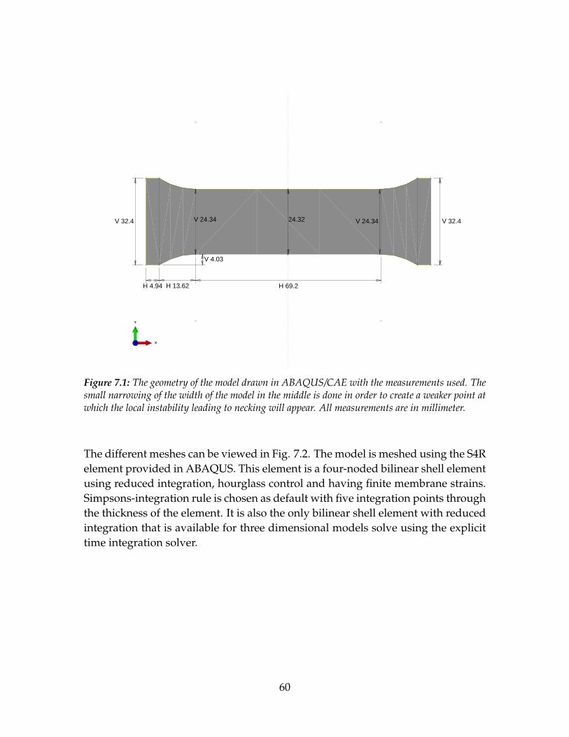
24.32

H 4.94

V 4.03

H 69.2

V 32.4V 24.34V 24.34

H 13.62

V 32.4

X

Y

Z

Figure 7.1: The geometry of the model drawn in ABAQUS/CAE with the measurements used. Thesmall narrowing of the width of the model in the middle is done in order to create a weaker point atwhich the local instability leading to necking will appear. All measurements are in millimeter.

The different meshes can be viewed in Fig. 7.2. The model is meshed using the S4Relement provided in ABAQUS. This element is a four-noded bilinear shell elementusing reduced integration, hourglass control and having finite membrane strains.Simpsons-integration rule is chosen as default with five integration points throughthe thickness of the element. It is also the only bilinear shell element with reducedintegration that is available for three dimensional models solve using the explicittime integration solver.

60

Viewport: 1 Model: Shell−2_2mm Part: Dog−Bone

RP

X

Y

Z

Viewport: 2 Model: Shell−4_4mm Part: Dog−Bone

RP

X

Y

Z

Viewport: 3 Model: Shell−8_8mm Part: Dog−Bone

RP

X

Y

Z

Viewport: 4 Model: Shell−17_6mm Part: Dog−Bone

RP

X

Y

Z

Figure 7.2: The four different meshes used on the dog-bone model.(Top left: 2.2 mm, Top right: 4.4mm, lower left: 8.8 mm, lower right: 17.6 mm) The model is meshed using edge seeds to define theside length of the elements in the middle part of the model, and the ends are seeded in order to keepa regular and well defined mesh.

The material is defined by its elastic properties, plastic properties and density1, anto be isotropic in its elastic properties, and to follow an isotropic strain-hardeningrule in the plastic properties. No field variables are used and the material is definedas independent of the temperature and the strain rate. The whole model is definedas being homogeneous.

The boundary conditions are chosen to best simulate the clamped ends on thetensile test piece when it is was stretched. One end (the left edge in Fig. 7.2) is

1The density is needed since the analysis is performed using a dynamic time integration solver(ABAQUS/Explicit). This option requires that the model has a mass, that is provided by the densityand the definition of a homogeneous material set in the Section module.

61

applied boundary conditions restraining all degrees of freedom, both translationand rotation, on all the nodes along the edge. In the other end (to the right in Fig.7.2) all the nodes along the edge are restrained against all translation and rotations,except the translation in the x-direction. This is kept free to be able to strain themodel. The elongation of the model is controlled by applying a constant velocityof +3.33333 mm/sec, in the x-direction, to the right side edge. This is the samevelocity as used in the FE-analysis performed in [11]. The velocity is applied tothe edge through a reference point, and a constrain forcing the edge of the modelto move in unison with the reference point in the x-direction. All of the boundaryconditions are applied to the geometry of the model, and not directly to the nodes.This makes it possible to change the mesh of the model without having to redefinethe regions of the boundary conditions.

The main outputs asked for in the analysis include energy magnitudes in the wholemodel, like the internal energy of the model, external work, and their energy com-ponents. Also the reaction force in the reference point and the reference point’sdisplacement. Each output is requested for 200 time steps, evenly spread out dur-ing the analysis.

The explicit dynamic analysis method is chosen when analyzing the models be-cause this is the most appropriate analyzing method to use on impact scenariosand collision analysis of thin walled structures [11]. In this case, the analysis canbe regarded as a quasi-static analysis. The ABAQUS documentation ([7] Sec. 6.3.3)recommend using the explicit analysis method for quasi-static analysis when thereis a contact definition between elements in use, like in the analysis performed inchapter 8.

The analysis is set to last for a total time period of 9 seconds, leading to a totalelongation of the model of 30 mm. Default values regarding incremental settingslike how to estimate the maximum stable increment, maximum time incrementallowed and time scaling are used. (For default values, please refer to the ABAQUSUser’s Manual ver. 6.11) Non-linear geometry is set to ON, allowing for geometricnon-linear effects to be included.

All the analysis regarding the tensile experiment and tuning of the material proper-ties is done using double precision. This means that the round of errors during theanalysis is reduced because more significant numbers are used to calculate eachincremental step. This influences the time used to run the analysis, increasing it

62

with up to 40 % as compared to running with single precision. The choice of usingdouble precision is made because this reduced the vibrations that occurred in themodel. Also, ABAQUS recommends that double precision is used when the totalnumber of time increments is larger than 300.000, or if the nodal displacement pertime increment is less than 10−6 times the corresponding nodel coordinate value([7] Sec. 6.1.1). Using double precision will always give a more accurate result thanusing single precision, at the cost of higher computational cost.

7.3 Development of the material models

For each of the different mesh sizes there was developed a material model usingthe method of Ehlers and Varsta (Sec. 5.2), and another using the damage criterionprovided in ABAQUS that is based on the method discussed in section 5.3. Thefirst material model will be referred to as the Plasticity material model (PMM), andthe later as the Damage Evolution material model (DEMM).

A total of eight FE-models are used to create the material models. Both the PMMand the DEMM were tuned using the dog-bone model presented in 7.2, with fourdifferent sized element meshes, using coarser meshes than used in [11]. This givesthe following FE-models:

• Four models using the Plasticity Material Model and mesh with elementshaving side lengths of 2.2 mm, 4.4 mm, 8.8 mm and 17.6 mm.

• Four models using the Damage Evolution Material Model and mesh withelements having side lengths of 2.2 mm, 4.4 mm, 8.8 mm and 17.6 mm.

In order to know that the behavior of the material was physically possible, andcan be related to the real world, the force-displacement curve produced in [11] wasused as a reference and control. The curve is shown in Fig. 7.3. This result is basedon the tensile test done on a 6 mm thick flat-bar dog-bone specimen made out ofREAX S275 LASER steel. This specimen showed a behavior of having its ultimatestrength after a global elongation of 17.5 mm. At the point of ultimate strength, thetrue strain in the elements, calculated as equivalent plastic strain, was 0.22.

63

Figure 7.3: The reference curve used to tune the tensile fracture model, taken from [11]. The crossmarks the point of global ultimate strength, and the assumed point of elongation where the structurecan support the maximum load.

The only difference between the FE-models used to develop the material modelsare the material models used (PMM and DEMM), plastic properties and the useof the damage model provided in ABAQUS. The elastic properties, the density ofthe material and the plastic properties of inserted true stress/true strain up to thepoint of 0.22 equivalent plastic strain, are the same for both of them.

7.3.1 Plasticity-model (PMM)

For the Plasticity-Material-Model (PMM) the global response regarding the force-displacement curve is tuned by an iterative procedure, using the plastic propertiesof the material to tune the true stress/true strain relationship for each of the el-ements in the model until the FE-model gives the same global response as thereference curve in Fig. 7.3. This is done for each of the four meshes sizes shown inFig. 7.2.

In order to achieve this global response, the plastic properties for the material hadto be tuned in such a way that the behavior of the elements in the model whencombined exerted the right stiffness in order to reproduce the global response. Upto the point of ultimate strength, when the true strain in the elements are about

64

0.22 all over, the plastic properties for each mesh size is equal. After the point ofultimate strength, when the true strain in the elements exceeds 0.22, the modelsdiffer depending on the mesh size. To get the right global response, the modelwas analyzed repeatedly, changing the plastic properties of the material in relationto the recorded output of the previous run. Since the response up to the point ofultimate strength were the same regardless of the element size, this part was tunedusing the 2.2 mm meshed FE-model, since this ensured most accuracy, withoutinterference from effects due to using large elements that could act stiffer thanthey should. The plastic behavior after the point of ultimate strength was tunedusing the different meshed models, and point by point dialing in the right valuesof true stress and true strain in order to get the right global response.

The final fracture, the reduction of applied force from the end point of the referencecurve in Fig. 7.2, was simulated using the Damage Initiation criterion and DamageEvolution for ductile materials, provided in ABAQUS, and was the same fracturemodel as used in the DEMM in section 7.3.2. The input data to the fracture modelwas obtained by running the model without this fracture criterion. Then the aver-age value of the equivalent plastic strain for the elements that are supposed to bedeleted, was measured at the point in time when the final fracture was supposedto happen. Then this strain value was used as the damage initiation criterion, anda linear damage evolution was defined. The fracture model data for the PMM areprovided in Table 7.1 in the result section.

7.3.2 Damage Evolution Material Model (DEMM)

The DEMM used the method presented in Section 5.3 in order to model the re-sponse after the ultimate strength. How the damage initiation criterion and thefollowing damage evolution works in ABAQUS is explained in Appendix A. Thismethod was used on the same differently meshed models as the PMM.

The behavior up to the point of ultimate strength was also here controlled by theelastic and plastic properties of the material. Therefore, the same data for elastic-ity and the plastic true stress/true strain relationship up to this point (when theεpl = 0.22) was used as for the PMM. Damage was initiated, using the damage ini-tiation criterion for ductile fracture provided in ABABQUS, at an equivalent plasticstrain value of 0.22. The point of damage initiation was set to be the same value

65

of equivalent strain for all of the different mesh sizes. After this point, the plas-tic properties for the material inputted was set to rise linearly following the sameslope as right before damage was initiated, towards an equivalent plastic strainvalue of 1.1413 at an equivalent stress value of 1100 MPa. This was done becausethe DEMM needs a true stress/true strain path σ that the material would have fol-lowed if it had not been damaged, since the damage true stress/true strain pathσ is defined by applying a damage parameter D so that σ = (1 − D)σ . See Ap-pendix A.3 for details about the damage parameter D. The data is inserted to thematerial model as a tabular relationship of the damage paramter D to the fracturedisplacement value upl.

Figure 7.4: The plastic properties used together with the DEMM. The plastic properties used thePMM for each of the four models in comparison.

This unphysical material behavior will never be followed by the FE-model, be-cause when the damage initiation criterion is breached by some of the elements ithe model, the other are being unloaded because the reduced stiffness of the ele-ments now following the damage evolution set by the fracture model is reducingthe load carrying capacity of the model.

After damage was initiated the damage evolution for each of the different meshedmodels was tuned using an iterative procedure until the force-displacement curvefor each of them matched the reference curve. The final tabular data used for thefour differently meshed models can be viewed in table 7.3, and the same tabular

66

data are plotted in Fig. 7.7.

7.4 Results and discussion

7.4.1 The material models

The four different meshed models used together with the two different materialmodels failed at a global elongation of of 27.75mm to 28 mm. In figure 7.5 theinitial deformation state and three other states of deformation are shown for the4.4 mm model.

Figure 7.5: Top left: The initial geometry of the dog-bone model. Top right: The deformation of themodel when it has reached its ultimate strength. Bottom left: The deformation state right before thefinal fracture caused by the elements being deleted. Bottom right: The final deformation, when theelement in the middle of the necking zone has been deleted.

67

The tuning of the global force-displacement curve for each of the differently meshedmodels, resulted in the PMM presented in Table 7.1 and the DEMM presented inTable 7.3. The data from these two tables are shown as graphic plots of the truestress/true stress for the PMM in Fig. 7.6 and as the relation of the damage pa-rameter D and the fracture displacement upl for the DEMM in Fig. 7.7. For all ofthe models, the same material data is used for the elastic behavior and the plasticbehavior up to the point of ultimate strength, when the true strain in the elementsis 0.22.

Table 7.1: The inputed stress-strain relationship for the PMM.

2.2 mm 4.4 mm 8.8 mm 17.6 mmStress Strain Stress Strain Stress Strain Stress Strain

340 0 340 0 340 0 340 0345 0.0393 345 0.0393 345 0.0393 345 0.0393380 0.0450 380 0.0450 380 0.0450 380 0.0450410 0.0550 410 0.0550 410 0.0550 410 0.0550450 0.0970 450 0.0970 450 0.0970 450 0.0970495 0.1413 495 0.1413 495 0.1413 495 0.1413545 0.2243 545 0.2243 545 0.2243 545 0.2243600 0.3300 585 0.3143 565 0.2763 585 0.3100640 0.4700 615 0.3800 590 0.3400 590 0.3450650 0.5300 625 0.4200 600 0.4000 570 0.3800655 0.6300 610 0.5700 550 0.5250 535 0.4200675 0.7000 600 0.5900 515 0.5450 505 0.4500720 0.9000740 1.1000

Since the PMM origionally does not include any form of fracture criterion, it waschosen to use the fracture model for ductile fracture in ABAQUS to simulate thefracture causing the drop in force seen in Fig. 7.8. This is the same procedurethat was used in [11] to make the model fracture, by deleting elements that havareached a certain value of equivalent plastic strain. The data used to make the dif-ferently meshed models fracture are given in Table 7.2. This data contains a dam-age initiation criterion for each mesh size that defines the equivalent true strainvalue an element must obtain before being deleted. The value of upl

f was set to beequal for all the different mesh sizes because this defines the global displacementof the model during the time step when the element is deleted. The value of theequivalent strain at the point of damage initiation was collected by first tuning theplasticity-model and then finding the appropriate equivalent strain value for thedamage initiation criterion. Then a damage evolution was set by defining a linear

68

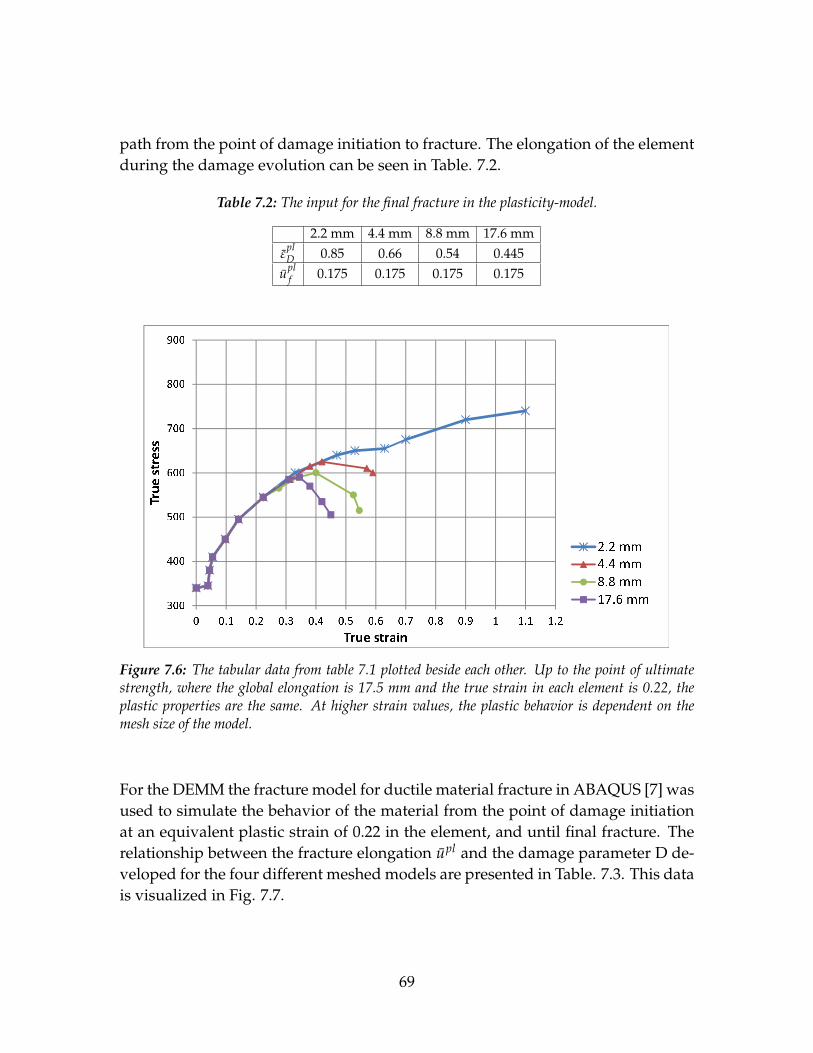
path from the point of damage initiation to fracture. The elongation of the elementduring the damage evolution can be seen in Table. 7.2.

Table 7.2: The input for the final fracture in the plasticity-model.

2.2 mm 4.4 mm 8.8 mm 17.6 mmε

plD 0.85 0.66 0.54 0.445

uplf 0.175 0.175 0.175 0.175

Figure 7.6: The tabular data from table 7.1 plotted beside each other. Up to the point of ultimatestrength, where the global elongation is 17.5 mm and the true strain in each element is 0.22, theplastic properties are the same. At higher strain values, the plastic behavior is dependent on themesh size of the model.

For the DEMM the fracture model for ductile material fracture in ABAQUS [7] wasused to simulate the behavior of the material from the point of damage initiationat an equivalent plastic strain of 0.22 in the element, and until final fracture. Therelationship between the fracture elongation upl and the damage parameter D de-veloped for the four different meshed models are presented in Table. 7.3. This datais visualized in Fig. 7.7.

69

Table 7.3: Tabular damage evolution data

2.2 mm 4.4 mm 8.8 mm 17.6 mmD upl D upl D upl D upl

0 0 0 0 0 0 0 00.070 0.700 0.059 1.000 0.0575 1.745 0.055 1.9500.160 1.050 0.170 1.500 0.0850 1.945 0.075 2.3500.215 1.450 0.250 1.900 0.1500 2.470 0.117 2.6000.240 1.800 0.310 2.180 0.27 3.000 0.240 3.4250.250 2.010 1 2.355 1 3.147 1 3.600

1 2.050

Figure 7.7: Plot of the tabular damage evolution data

At the point of ultimate strength, when the true strain in the elements are 0.22,the different meshed FE-models starts to behave different from each other. Themodels with the largest elements behave more stiffly than the models with smallerelements. For the PMM, the true stress/true strain relationship had to be tunedin accordence with this. The softer behavior of the fine meshed models is causedby the effect of the fine meshed FE-models obtaining a larger true strain in theelements than the coarser meshed models, when exposed to the same absoluteelongation, as explained in Section 5.1.

70

The global force-displacement curve, produced by the FE-models using the mate-rial data provided in Table 7.1 and 7.2 for the PMM, and Table 7.3 for the DEMM,is seen i Fig. 7.8 and 7.9.

The 2.2 mm FE-model using the PMM shows a much softer behavior than theother FE-models, and the resulting true stress/true strain relationship is differentin shape compared to the coarser meshed FE-models. This is caused by the 2.2mm meshed FE-model actually being, to some degree, capable of simulating theinstability caused by the δσ/δε ration becoming larger than the true stress in theelements, as explained in Section 3.1. This derives from the fact that the 2.2 mmFE-model is meshed with enough elements in the width of the model, giving itthe capability to locally simulate the reduction in cross-section area responsiblefor causing the instability, as the strain hardening effect of the material becomesweaker. This is why the 2.2 mm meshed PMM FE-model develops a different truestress/true strain relationship, seen in Fig. 7.6 than the coarser meshed models.Only a small dent in the curve is needed to make the material behave in sucha way that the global responce of the model follows the reference curve in Fig.7.3. If we look back on the results from Ehlers and Varstas experiments in [11],shown in Fig. 5.4, the same effect can be recognized as applied to their simulation.They used much finer meshed models, and did not pass over the threshold wherethe small number of elements in the transverse direction prevented the FE-modelfrom being able to simulate the reduction of the cross-section area. This meantthat they did not have to create a drop in the materials’ plastic stiffness in orderto manipulate the model into following the global response seen from the tensiletest they performed. The three other FE-models used in the experiments in thisthesis are on the other hand more coarsely meshed, and this makes them lose theability to simulate the necking just from the mesh alone. This effect was insteadincorporated into the material definition itself, by letting the true stress/true straincurve for the PMM shown in Fig. 7.6 to drop. The larger the elements in the modelare, the more stiffly it behaves. So the coarse mesh PMM FE-models must havea softer material behavior after the point of element ultitmate strength,in order togive the same global response regarding the force and deformation.

As for the PMM, the 2.2 mm mesh FE-model with the DEMM show a differentbehavior than the three other coarser meshed DEMM FE-models. Since this FE-model has the capability to simulate the effect of necking to some degree with-out altering the material, it already has a softer response than the other three FE-models using the DEMM. The models meshed with 4.4 mm to 17.6 mm element

71

Figu

re7.

8:Th

eres

ultin

gfo

rce-

disp

lace

men

tcur

vesf

orth

ediff

eren

tmes

hsi

zesw

hen

tune

dag

ains

tthe

forc

e-di

spla

cem

entc

urve

prov

ided

in[1

1].

The

curv

ew

ithth

em

arks

defin

esth

ere

fere

nce

curv

e.Th

epo

into

fulti

mat

est

reng

this

atth

eve

rtex

ofth

ecu

rves

,afte

ran

elon

gatio

nof

appr

oxim

atel

y17

.75

mm

.

72

Figu

re7.

9:Th

eres

ultin

gfo

rce-

disp

lace

men

tcur

vesf

orth

ediff

eren

tmes

hsi

zesw

hen

tune

dag

ains

tthe

forc

e-di

spla

cem

entc

urve

prov

ided

in[1

1].

The

curv

ew

ithth

em

arks

defin

esth

ere

fere

nce

curv

e.Th

epo

into

fulti

mat

est

reng

this

atth

eve

rtex

ofth

ecu

rves

,afte

ran

elon

gatio

nof

appr

oxem

ently

17.7

5m

m.

73

size are not capable of displaying the effect of the cross-section area being reducedenough to give necking as the true strain in the elements increase. This effect willcome first at a higher strain value, giving it the wrong global response. As for themodels using the PMM, the effect of instability is instead simulated by reducingthe true stress value in the elements as the true strain increases.

For the DEMM, the reduction in strength in each element is not caused by lower-ing the true stress to true strain relationship. It is done by reducing the true stressvalues for a given true strain value in the plastic properties of the material with afactor called the damage parameter D. The inputted true stress/true strain definesa path σ (see Fig. 7.4) that the elements would follow if not influenced by the dam-age initiation criterion. If the elements trigger the damage initiation criterion theelement will follow a true stress/true strain path where the true stress is definedas σ = (1− D)σ . At the same time, the elastic stiffness of the element is reducedwith a factor (1− D), as the fracture elongation upl increases from 0 to upl

f .

7.4.2 Comparing energy components

The two material models (PMM and DEMM) for the four different mesh sizes showgood agreement between the global response of the FE-model and the global re-sponse of the tensile test performed in [11].

Since the FE-models are tuned to give the same amount of displacement for a givenforce using different mesh sizes and material input, the energies quantities in thematerial should be the same for all the different cases, they were monitored tomake sure that no strange effects occur that may influence the result. The ABAQUSUser’s Manual recommends monitoring the energy quantities in the whole modelto look for unexpected changes in the energy components of the model. A discus-sion of the different energy quantities follows.

The first check is that the internal energy should be matched by the external workapplied to the model. In this analysis the external work is given as the force ap-plied to the model multiplied by the elongation of the model in the direction ofthe force. Since the analysis is done using a constant speed giving a constantlygrowing elongation the external work is set to increase following a path definedby the elongation and the force needed to apply the deformation. Fig. 7.10 shows

74

the external work, comparing the PMM against the DEMM for the four differentmeshed models.

Figure 7.10: The external work performed on the models.

The internal energy should be the same as the external work, because there is noadditional energy applied than the force giving the elongation, and there shouldnot be any energy lost. Fig. 7.11 shows the internal energy, comparing the PMMagainst the DEMM for the four differently meshed models. The external work andthe internal energy are in good agreement with each other, but the energy calcu-lated by ABAQUS is not exactly equal, showing a difference of 0.1 % between theextrenal work and the interna energy. The energy missing in the internal energy iscaused by the dissipation of energy to viscous damping and kinetic energy, causedby using a dynamic solver to solve the problem. Also, some energy is unaccountedfor, and this amount of energy is added to the energy balance as a residual amount.Adding the energy lost to viscose dampening and the kinetic energy, and subtract-ing the residual energy from the given internal energy, produces the same result asthe external work calculated by ABAQUS. This means that all of the energy addedto the system is accounted for.

75

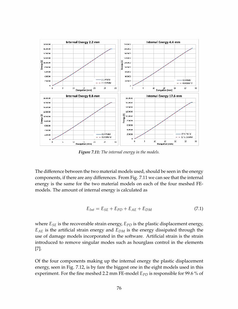
Figure 7.11: The internal energy in the models.

The difference between the two material models used, should be seen in the energycomponents, if there are any differences. From Fig. 7.11 we can see that the internalenergy is the same for the two material models on each of the four meshed FE-models. The amount of internal energy is calculated as

EInt = ESE + EPD + EAE + EDM (7.1)

where ESE is the recoverable strain energy, EPD is the plastic displacement energy,EAE is the artificial strain energy and EDM is the energy dissipated through theuse of damage models incorporated in the software. Artificial strain is the strainintroduced to remove singular modes such as hourglass control in the elements[7].

Of the four components making up the internal energy the plastic displacementenergy, seen in Fig. 7.12, is by fare the biggest one in the eight models used in thisexperiment. For the fine meshed 2.2 mm FE-model EPD is responsible for 99.6 % of

76

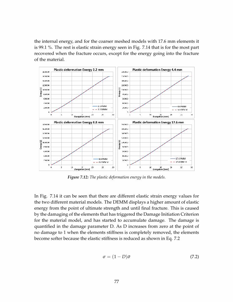
the internal energy, and for the coarser meshed models with 17.6 mm elements itis 99.1 %. The rest is elastic strain energy seen in Fig. 7.14 that is for the most partrecovered when the fracture occurs, except for the energy going into the fractureof the material.

Figure 7.12: The plastic deformation energy in the models.

In Fig. 7.14 it can be seen that there are different elastic strain energy values forthe two different material models. The DEMM displays a higher amount of elasticenergy from the point of ultimate strength and until final fracture. This is causedby the damaging of the elements that has triggered the Damage Initiation Criterionfor the material model, and has started to accumulate damage. The damage isquantified in the damage parameter D. As D increases from zero at the point ofno damage to 1 when the elements stiffness is completely removed, the elementsbecome softer because the elastic stiffness is reduced as shown in Eq. 7.2

σ = (1− D)σ (7.2)

77

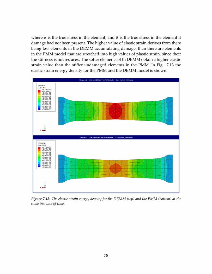
where σ is the true stress in the element, and σ is the true stress in the element ifdamage had not been present. The higher value of elastic strain derives from therebeing less elements in the DEMM accumulating damage, than there are elementsin the PMM model that are stretched into high values of plastic strain, since theirthe stiffness is not reduces. The softer elements of th DEMM obtain a higher elasticstrain value than the stiffer undamaged elements in the PMM. In Fig. 7.13 theelastic strain energy density for the PMM and the DEMM model is shown.

Viewport: 1 ODB: I:/MASTEROPPGAVE/TENSILE ... − Siste Uke/4_4−DEMM.odb

(Avg: 75%)ESEDEN

+0.000e+00+9.800e−02+1.960e−01+2.940e−01+3.920e−01+4.900e−01+5.880e−01+6.860e−01+7.840e−01+8.820e−01+9.800e−01+1.078e+00+1.176e+00

X

Y

Z

Viewport: 2 ODB: I:/MASTEROPPGAVE/TENSILE ...l − Siste Uke/4_4−PMM.odb

(Avg: 75%)ESEDEN

+0.000e+00+9.800e−02+1.960e−01+2.940e−01+3.920e−01+4.900e−01+5.880e−01+6.860e−01+7.840e−01+8.820e−01+9.800e−01+1.078e+00+1.176e+00

X

Y

Z

Figure 7.13: The elastic strain energy density for the DEMM (top) and the PMM (bottom) at thesame instance of time.

78

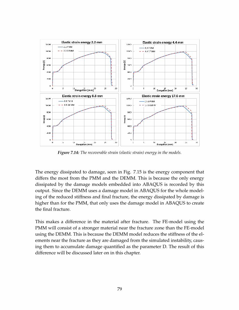
Figure 7.14: The recoverable strain (elastic strain) energy in the models.

The energy dissipated to damage, seen in Fig. 7.15 is the energy component thatdiffers the most from the PMM and the DEMM. This is because the only energydissipated by the damage models embedded into ABAQUS is recorded by thisoutput. Since the DEMM uses a damage model in ABAQUS for the whole model-ing of the reduced stiffness and final fracture, the energy dissipated by damage ishigher than for the PMM, that only uses the damage model in ABAQUS to createthe final fracture.

This makes a difference in the material after fracture. The FE-model using thePMM will consist of a stronger material near the fracture zone than the FE-modelusing the DEMM. This is because the DEMM model reduces the stiffness of the el-ements near the fracture as they are damaged from the simulated instability, caus-ing them to accumulate damage quantified as the parameter D. The result of thisdifference will be discussed later on in this chapter.

79

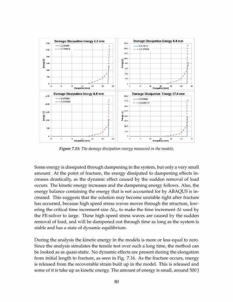
Figure 7.15: The damage dissipation energy measured in the models.

Some energy is dissipated through dampening in the system, but only a very smallamount. At the point of fracture, the energy dissipated to dampening effects in-creases drastically, as the dynamic effect caused by the sudden removal of loadoccurs. The kinetic energy increases and the dampening energy follows. Also, theenergy balance containing the energy that is not accounted for by ABAQUS is in-creased. This suggests that the solution may become unstable right after fracturehas occurred, because high speed stress waves moves through the structure, low-ering the critical time increment size ∆tcr to make the time increment ∆t used bythe FE-solver to large. These high speed stress waves are caused by the suddenremoval of load, and will be dampened out through time as long as the system isstable and has a state of dynamic equilibrium.

During the analysis the kinetic energy in the models is more or less equal to zero.Since the analysis simulates the tensile test over such a long time, the method canbe looked as as quasi-static. No dynamic effects are present during the elongationfrom initial length to fracture, as seen in Fig. 7.16. As the fracture occurs, energyis released from the recoverable strain built up in the model. This is released andsome of it is take up as kinetic energy. The amount of energy is small, around 500 J

80

(while the total internal energy is 1.6 MJ), expect for the 4.4 mm model using PMM.Here the kinetic energy peaks at just short of 5000 J. This is probably caused by theform of the true stress/true strain inputted in the material data. The 17.6 mm and8.8 mm PMM has a steeper drop in stiffness as the strain in the material closesin on the point of final failure. The 4.4 mm PMM has a more gently slop whenreducing the stiffness as it nears the final failure, giving it little higher stress valuein the material when i finally fractures. The higher stress value being removedintroduces higher post-failure dynamics effects as kinetic energy and dampeningin the system.

Figure 7.16: The kinetic energy measured in the models

From the discussion of the energy components there are only small difference be-tween the two material models when used on the same mesh size. The material istuned to give the same response regarding force and displacement, so a differencein the total energy would have been surprising, and does not happen. The only no-ticeable difference is the damage dissipation energy, and the elastic strain energy.These behave differently from the point of ultimate strength to final fracture. ThePMM model has a lower value of recoverable strain than the DEMM. This derivesfrom the reduction of strength in the elements exposed to damage in the DEMM

81

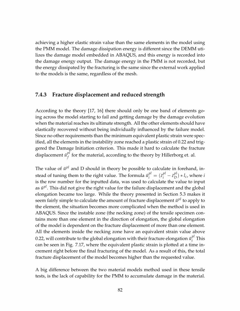
achieving a higher elastic strain value than the same elements in the model usingthe PMM model. The damage dissipation energy is different since the DEMM uti-lizes the damage model embedded in ABAQUS, and this energy is recorded intothe damage energy output. The damage energy in the PMM is not recorded, butthe energy dissipated by the fracturing is the same since the external work appliedto the models is the same, regardless of the mesh.

7.4.3 Fracture displacement and reduced strength

According to the theory [17, 16] there should only be one band of elements go-ing across the model starting to fail and getting damage by the damage evolutionwhen the material reaches its ultimate strength. All the other elements should haveelastically recovered without being individually influenced by the failure model.Since no other requirements than the minimum equivalent plastic strain were spec-ified, all the elements in the instability zone reached a plastic strain of 0.22 and trig-gered the Damage Initiation criterion. This made it hard to calculate the fracturedisplacement upl

f for the material, according to the theory by Hillerborg et. al.

The value of upl and D should in theory be possible to calculate in forehand, in-stead of tuning them to the right value. The formula upl

i = (εpli − ε

plD ) ∗ lc, where i

is the row number for the inputted data, was used to calculate the value to inputas upl. This did not give the right value for the failure displacement and the globalelongation became too large. While the theory presented in Section 5.3 makes itseem fairly simple to calculate the amount of fracture displacement upl to apply tothe element, the situation becomes more complicated when the method is used inABAQUS. Since the instable zone (the necking zone) of the tensile specimen con-tains more than one element in the direction of elongation, the global elongationof the model is dependent on the fracture displacement of more than one element.All the elements inside the necking zone have an equivalent strain value above0.22, will contribute to the global elongation with their fracture elongation upl

i Thiscan be seen in Fig. 7.17, where the equivalent plastic strain is plotted at a time in-crement right before the final fracturing of the model. As a result of this, the totalfracture displacement of the model becomes higher than the requested value.

A big difference between the two material models method used in these tensiletests, is the lack of capability for the PMM to accumulate damage in the material.

82

When using the DEMM, there is accumulated damage in the elements that has trig-gered the damage initiation criterion and therefore follows the fracture model ofHillersborg et. al. The damage to each element is quantified by the damage param-eter D, and the load bearing capacity of the element is reduced by a factor (1−D).If the element according to the inputted true stress/true strain relationship for theplastic area should be able to carry a load σ when its equivalent plastic strain isε, the damage element can only carry σ = (1 − D)σ . Also, the elastic stiffnessof the element is reduced by the same factor (1 − D). This reduction of elementstiffness is permanent, and can not be reversed. The PMM, as presented by Ehlersand Varsta in [11], does not include any damage parameter. In their model, thereduced stiffness is a result of the reduced value of true stress as the plastic strainincreases (see Fig. 7.4), but this effect can be reversed by reversing the loading onthe material, since there is no damage applied to the material of the elements whenthey pass their ultimate loading. In the tensile experiments, the damage inflictedto elements that were not deleted was up to 16 % reduction of elastic stiffness, inthe DEMM. For the PMM no elements, except for the one that got deleted, wereinflicted by any damage, and the elastic stiffness of the remaining material waspreserved.

83

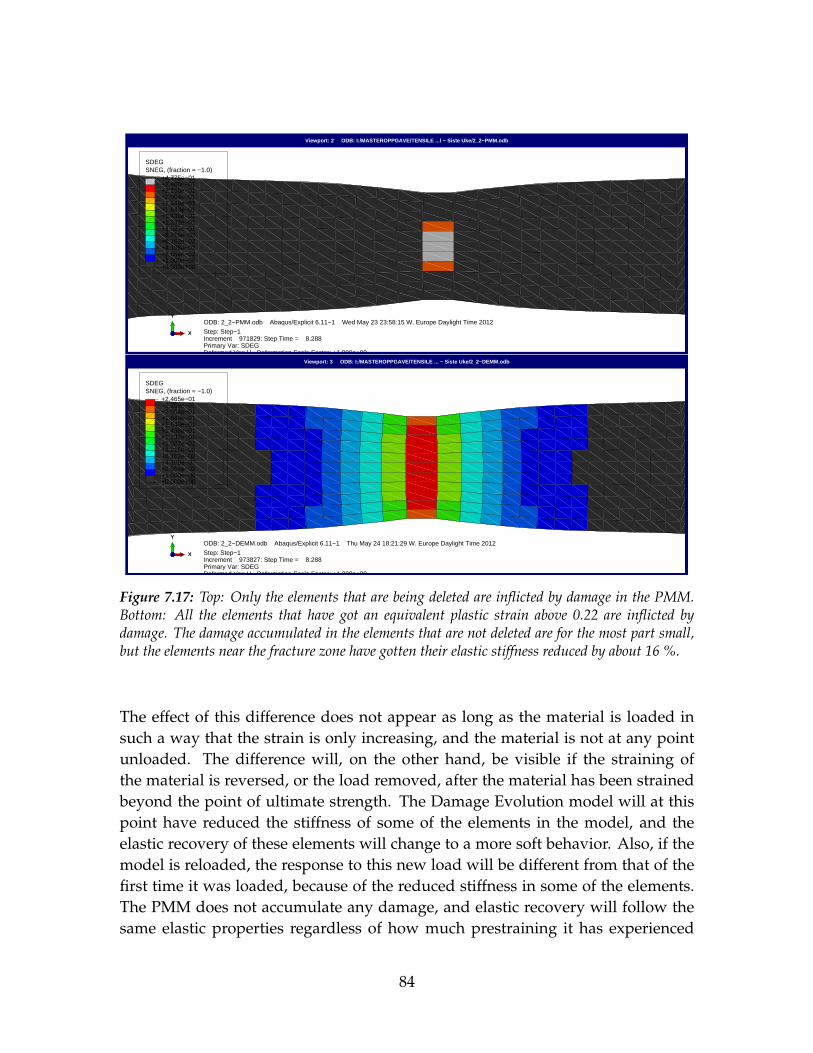
Viewport: 3 ODB: I:/MASTEROPPGAVE/TENSILE ... − Siste Uke/2_2−DEMM.odb

SNEG, (fraction = −1.0)SDEG

+1.000e−06+2.054e−02+4.108e−02+6.162e−02+8.216e−02+1.027e−01+1.232e−01+1.438e−01+1.643e−01+1.849e−01+2.054e−01+2.259e−01+2.465e−01

+0.000e+00

Step: Step−1Increment 973827: Step Time = 8.288Primary Var: SDEGDeformed Var: U Deformation Scale Factor: +1.000e+00

ODB: 2_2−DEMM.odb Abaqus/Explicit 6.11−1 Thu May 24 18:21:29 W. Europe Daylight Time 2012

X

Y

Z

Viewport: 2 ODB: I:/MASTEROPPGAVE/TENSILE ...l − Siste Uke/2_2−PMM.odb

SNEG, (fraction = −1.0)SDEG

+1.000e−06+2.054e−02+4.108e−02+6.162e−02+8.216e−02+1.027e−01+1.232e−01+1.438e−01+1.643e−01+1.849e−01+2.054e−01+2.259e−01+2.465e−01

+0.000e+00

+4.775e−01

Step: Step−1Increment 971829: Step Time = 8.288Primary Var: SDEGDeformed Var: U Deformation Scale Factor: +1.000e+00

ODB: 2_2−PMM.odb Abaqus/Explicit 6.11−1 Wed May 23 23:58:15 W. Europe Daylight Time 2012

X

Y

Z

Figure 7.17: Top: Only the elements that are being deleted are inflicted by damage in the PMM.Bottom: All the elements that have got an equivalent plastic strain above 0.22 are inflicted bydamage. The damage accumulated in the elements that are not deleted are for the most part small,but the elements near the fracture zone have gotten their elastic stiffness reduced by about 16 %.

The effect of this difference does not appear as long as the material is loaded insuch a way that the strain is only increasing, and the material is not at any pointunloaded. The difference will, on the other hand, be visible if the straining ofthe material is reversed, or the load removed, after the material has been strainedbeyond the point of ultimate strength. The Damage Evolution model will at thispoint have reduced the stiffness of some of the elements in the model, and theelastic recovery of these elements will change to a more soft behavior. Also, if themodel is reloaded, the response to this new load will be different from that of thefirst time it was loaded, because of the reduced stiffness in some of the elements.The PMM does not accumulate any damage, and elastic recovery will follow thesame elastic properties regardless of how much prestraining it has experienced

84

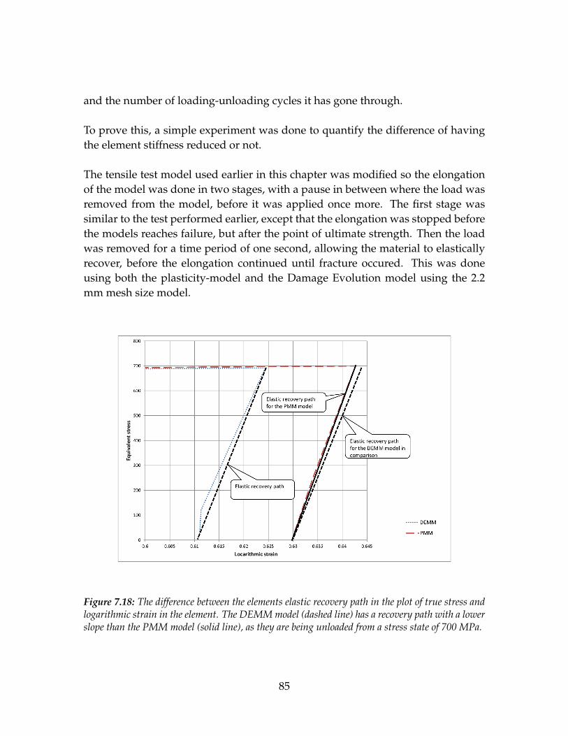
and the number of loading-unloading cycles it has gone through.

To prove this, a simple experiment was done to quantify the difference of havingthe element stiffness reduced or not.

The tensile test model used earlier in this chapter was modified so the elongationof the model was done in two stages, with a pause in between where the load wasremoved from the model, before it was applied once more. The first stage wassimilar to the test performed earlier, except that the elongation was stopped beforethe models reaches failure, but after the point of ultimate strength. Then the loadwas removed for a time period of one second, allowing the material to elasticallyrecover, before the elongation continued until fracture occured. This was doneusing both the plasticity-model and the Damage Evolution model using the 2.2mm mesh size model.

Figure 7.18: The difference between the elements elastic recovery path in the plot of true stress andlogarithmic strain in the element. The DEMM model (dashed line) has a recovery path with a lowerslope than the PMM model (solid line), as they are being unloaded from a stress state of 700 MPa.

85

By looking at the same element, located in the center of the necking zone, we cansee in Fig. 7.18 that the element recover elastically differently in the two models.The element using the DEMM recover elastically using a lower elastic stiffnessthan the element using the PMM. The Young’s-modulus that the elements use torecover elastically can be calculated as

E =δσ

δε(7.3)

where δσ is the reduction in equivalent stress in the element when it is unloaded,and δε is the corresponding reduction in logarithmic strain.

This gives E = 49700MPa for the element using the DEMM, and E = 57453MPafor the element using the PMM. The initial Young’s-modulus was 57500 MPa2.At the same time the damage parameter for the element using the DEMM wasmeasured to be 0.1324. Since the element stiffness is reduced by the factor (1− D)

this gives us a reduced elastic stiffness of

57500MPa(1− 0.1324) = 49887MPa (7.4)

for the DEMM, matching the elastic strain recovery stiffness measured in the plotin Fig. 7.18

7.4.4 Final comments to the results

The goal of this experiment was to understand and use the two different ma-terial models, the Plasticity-Material-Model (PMM) and the Damage Evolution-Material-Model (DEMM), to developed material models use in a fracture exper-iment on a plate. The material models develop to for the four different meshedFE-models will in the next chapter be used in a penetration experiment to get moredata on the differences between the two approaches, in order to be able to simu-

2The Young’s-modulus for this experiment was set to a lower value than normal because itwould be easier to measure the difference in the slope of the unloading path with the materialacting more softly than normal.

86

late the local instability that occurs during a ductile fracture, using as large finiteelements as possible.

87

Chapter 8

Plate penetration experiment inABAQUS

8.1 Introduction

In this chapter the analysis of a circular plate being penetrated by a cone-shapedpuncher is presented. The aim of this experiment is to search for significant dif-ferences between using the two material models presented in the prior chapter ondifferent meshed models using relatively large elements in order to save compu-tation time. The material data to be used is the material models created for thedifferent meshed FE-models in the tensile test experiment presented in chapter 7.The fracture of the steel plate is assumed to be governed by the ductile tensile frac-ture behavior of the steel material, as this is the type of fracture the material modelsare tuned for. Other types of fracture, if they should occur in such an experiment,are neglected.

This experiment is based on the experiment carried out by Sören Ehlers [10], butlike in the tensile test experiment, the mesh size used here has larger elements.This is done, as explained earlier, because it is desirable to use as large elementsas possible when modeling huge structures that are supposed to obtain damagein e.g. collision events. This is desirable because the analysis is solved using anexplicit time integration solver, and the computation time is directly linked to thesize of the smallest elements in the model.

88

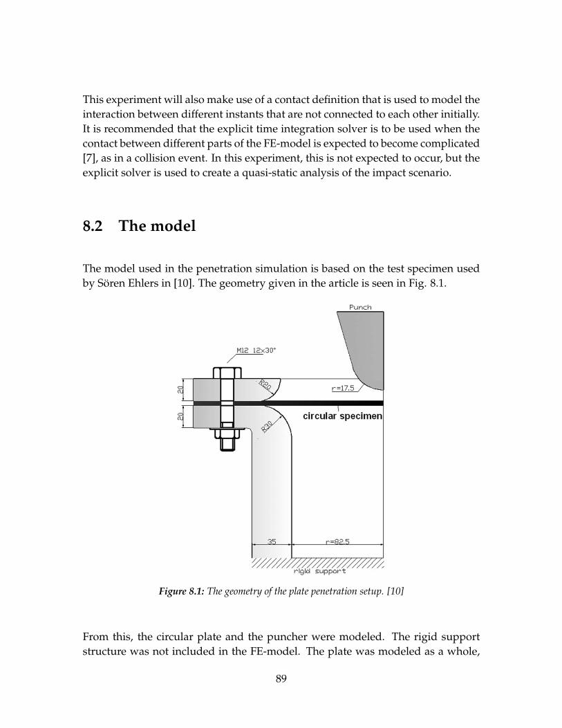
This experiment will also make use of a contact definition that is used to model theinteraction between different instants that are not connected to each other initially.It is recommended that the explicit time integration solver is to be used when thecontact between different parts of the FE-model is expected to become complicated[7], as in a collision event. In this experiment, this is not expected to occur, but theexplicit solver is used to create a quasi-static analysis of the impact scenario.

8.2 The model

The model used in the penetration simulation is based on the test specimen usedby Sören Ehlers in [10]. The geometry given in the article is seen in Fig. 8.1.

Figure 8.1: The geometry of the plate penetration setup. [10]

From this, the circular plate and the puncher were modeled. The rigid supportstructure was not included in the FE-model. The plate was modeled as a whole,

89

including the part being clamped by the test rig, but not the holes used to bolt theplate to the test rig model. The plate’s dimensions can be seen in Fig. 8.2. The totalradius is 170 mm, while the radius of the part of the plate inside the clamped rim is112.5 mm. The squared region in the middle of the plate measures 114.55 by 114.55mm, and is enclosed by a circle with a radius of 81 mm. The thickness of the plateis the same as in [10], 4.12 mm. The mesh of the model was supposed to be equal tothe mesh of the tensile test models, in order to use the material models developedthere. To get a quadratic mesh in the center of the plate where the contact betweenthe puncher and the plate would be, a squared partition was made in order togive a quadratic mesh in the center. The squared middle section lies so that thecorners are on the circle surrounding it. The circle segment in between is meshedin a way that gives it a mesh of S4R elements with the least possible distortion ofthe elements. For the 8.8 mm, 4.4 mm and 2.2 mm sized meshed element models,these segments had to be divided into two equal parts in order to keep the meshsymmetrical. The outer rim of the plate was meshed with the same element type,using a radial mesh control. According to Ehlers [10] this way of meshing theplate model secures the right dimensions of the element mainly responsible forsimulating the deformation of the plate and the elements simulating the rim beingclamped to the test rig.

Boundary conditions defining the clamped rim were applied to the outer sectionof the plate seen in Fig. 8.2, constraining all degrees of freedom in this part of themodel. The boundary conditions were applied to the geometry of the plate, andnot the mesh, as this made it possible to change the mesh of the model withouthaving to redefine the boundary conditions.

90

Figure 8.2: The geometry of the circular plate used in the FE-model.

The puncher was made as a discrete rigid surface. This means that the surfacewill not be able to deform, and will keep its initial shape throughout the analysis.The discrete rigid surface is defined by a mesh of undeformable elements. Havingelements containing nodes is beneficial when the contact between the surfaces ofthe two parts are to be defined. This saves computation time when running theanalysis. Alternatively, an analytical rigid surface could have been used. This is arigid surface that is defined by the geometry, and not a mesh of rigid elements asthe discrete rigid surface. This will make the computer analysis run more slowly,since the geometrically defined surface is more complicated to analyze than themeshed surface of the discrete rigid body. A test performed on the 4.4 mm meshedplate, using the DEMM, did not show any significant differences in the results ofthe plate being penetrated.

The dimensions of the puncher were only given in [10] by the radius of the roundedend. The figure clearly showed an angle side surface, but the details were not spec-ified. The angle of this sloping surface and a horizontal plane was assumed to be74◦, from measurements taken from Fig. 8.1. The spherical tip has a height of12.7 mm, and a radius of 17.5 mm. The total height of the puncher was set to 49mm. This ensured that the puncher did not pass all the way through the plate.In order to ensure that the puncher moved through the plate perpendicular to theplate’s initial surface, the reference point of the puncher was restrained against allmovements and rotations except for the translation in the global y-direction, per-pendicular to the plane of the plate. A constant speed of −3.33333 mm/sec was

91

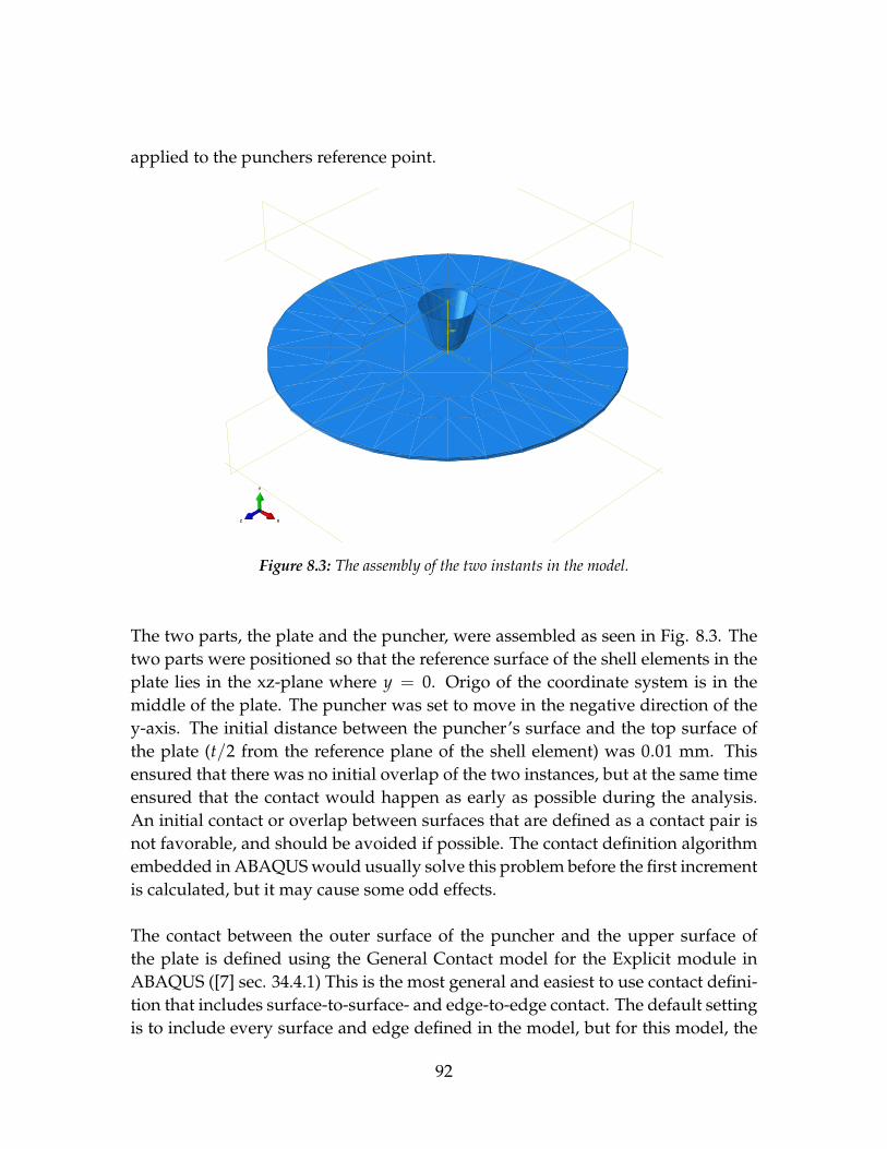
applied to the punchers reference point.

Z

Y

X

RP

X

Y

Z

Figure 8.3: The assembly of the two instants in the model.

The two parts, the plate and the puncher, were assembled as seen in Fig. 8.3. Thetwo parts were positioned so that the reference surface of the shell elements in theplate lies in the xz-plane where y = 0. Origo of the coordinate system is in themiddle of the plate. The puncher was set to move in the negative direction of they-axis. The initial distance between the puncher’s surface and the top surface ofthe plate (t/2 from the reference plane of the shell element) was 0.01 mm. Thisensured that there was no initial overlap of the two instances, but at the same timeensured that the contact would happen as early as possible during the analysis.An initial contact or overlap between surfaces that are defined as a contact pair isnot favorable, and should be avoided if possible. The contact definition algorithmembedded in ABAQUS would usually solve this problem before the first incrementis calculated, but it may cause some odd effects.

The contact between the outer surface of the puncher and the upper surface ofthe plate is defined using the General Contact model for the Explicit module inABAQUS ([7] sec. 34.4.1) This is the most general and easiest to use contact defini-tion that includes surface-to-surface- and edge-to-edge contact. The default settingis to include every surface and edge defined in the model, but for this model, the

92

Table 8.1: Contact pairs used in the plate penetration experiment.

Surface 1 Surface 2 Contact typePlate - Upper surface Plate - Upper surface Self-contactPlate - Upper surface Puncher - Outer surface Surface-to-surfacePucher - Outer surface Puncher - Outer surface Self-contact

surfaces were picked manually, as they are clearly defined. This saves time whenrunning the analysis because elements and nodes that are sure not to participatein the contact can be left out from the calculations. The surfaces included in thecontact definition are defined as surfaces in the FE-model. Both surface-to-surfaceand self-contact were defined for the surface of the puncher and the top surface ofthe plate-elements.

In short terms, the contact between the surfaces is modeled by monitoring thenodes of both surfaces, and calculating if they are in contact or not. If a nodeon one surface is found to be penetrating the surface of the other object, a forcejust large enough to push the node back to the surface of the penetrated object isapplied. This small force and displacement creates a small amount of work that isrecorded as penalty contact work.

As for the tensile test experiment, double numerical precision was chosen, in or-der to reduce the vibrations that by experience can occur during such an analysis.Also, the number of increments used to calculate some of the finer meshed platesexceeds 300 000, and the software documentations recommend to use double pre-cision when this happens.

8.3 Analysis

The analysis was done using the PMM and the DEMM on four different meshedplates. The objective was to use the same element size in the center region of theplate, as the mesh in the tensile test experiment in Chapter 7. Therefore, a quadraticshaped area was created in the contact zone that was meshed using (geometrically)quadratically shaped elements. The element sizes chosen were 2.2 mm, 4.4 mm, 8.8mm and 17.6 mm, the same as in the tensile test in Chapter 7, matching the materialinput used. The different meshed models are seen in Fig. 8.4.

93

The analysis was performed using the dynamic explicit time integration solver,for the same reasons as in the tensile test, and was run for an analysis time of15 seconds. This gives a total displacement of the puncher of 50 mm. All of theanalysis was performed using double precision. This choice was made because thehigh number of increments demanded by the finer meshed models would havemade the single precision accuracy too vulnerable for instability due to round offerrors.

Viewport: 4 Model: 17_6mm − DE Part: Deformeble plate

X

Y

Z

Viewport: 3 Model: 8_8mm − DE Part: Deformeble plate

X

Y

Z

Viewport: 2 Model: 4_4mm − DE Part: Deformeble plate

X

Y

Z

Viewport: 1 Model: 2_2mm − DE Part: Deformeble plate

X

Y

Z

Figure 8.4: The mesh used in the plate puncture simulation. Top left: 2.2 mm mesh, Top right: 4.4mm mesh, Bottom left: 8.8 mm mesh and bottom right: 17.6 mm mesh.

Output was requested for the displacement and the reaction force in the refer-ence point of the puncher. These were used to evaluate the analysis against theforce-displacement curve that was developed in the penetration tests performedby Sören Ehlers in [10]. For the deformable plate, all energy magnitudes for thewhole model were outputted, while the strain measurements, stress parametersand different damage related parameters of each element were outputted as a fieldoutput.

94

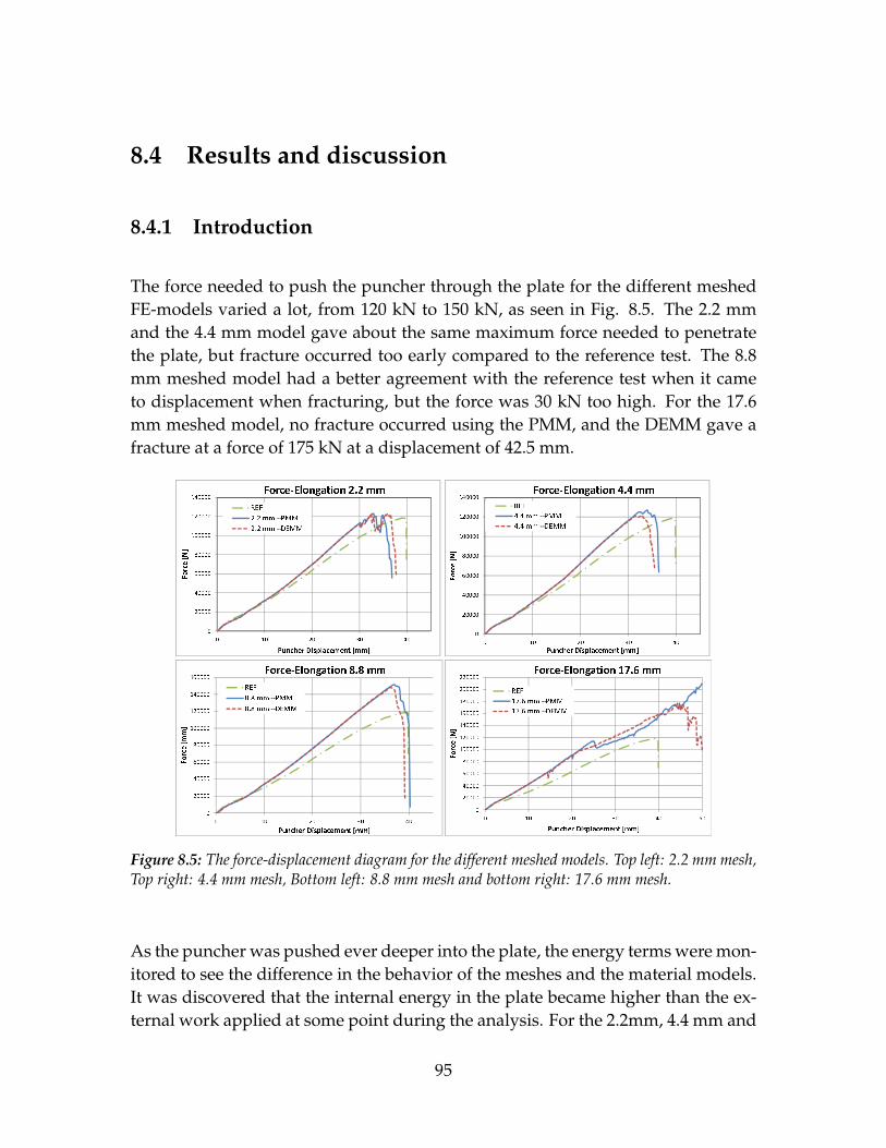
8.4 Results and discussion

8.4.1 Introduction

The force needed to push the puncher through the plate for the different meshedFE-models varied a lot, from 120 kN to 150 kN, as seen in Fig. 8.5. The 2.2 mmand the 4.4 mm model gave about the same maximum force needed to penetratethe plate, but fracture occurred too early compared to the reference test. The 8.8mm meshed model had a better agreement with the reference test when it cameto displacement when fracturing, but the force was 30 kN too high. For the 17.6mm meshed model, no fracture occurred using the PMM, and the DEMM gave afracture at a force of 175 kN at a displacement of 42.5 mm.

Figure 8.5: The force-displacement diagram for the different meshed models. Top left: 2.2 mm mesh,Top right: 4.4 mm mesh, Bottom left: 8.8 mm mesh and bottom right: 17.6 mm mesh.

As the puncher was pushed ever deeper into the plate, the energy terms were mon-itored to see the difference in the behavior of the meshes and the material models.It was discovered that the internal energy in the plate became higher than the ex-ternal work applied at some point during the analysis. For the 2.2mm, 4.4 mm and

95

the 8.8 mm meshed models, this happened as the fracture happened, changing theanalysis from an assumed quasi-static analysis into a dynamic analysis with largevibrations. For the 17.6 mm meshed model, this transition happened earlier thanfor the other mesh sizes. This is discussed in Section 8.4.2

During the whole analysis, the external work applied to the plate was defined as

WExt = Fu = EInt + EKE + EFric (8.1)

where F is the force, u is the puncher’s displacement causing the deformation ofthe plate, EKe is the kinetic energy in the plate, EFric is the energy lost to frictionand EInt is the internal energy in the plate. As long as no rupture of the plate hadoccurred, the analysis behaved quasi-static, without any dynamic effects present.The EKe was zero and EFric was very small. This meant that the external work wasmatched by the internal energy, and all the work applied to the system went intodeforming the plate elastically and plastically. When the problem being solvedbecame a dynamic case, this could be seen as a rise in the kinetic energy fromvibrations occurring in the structure. This introduced viscous dampening effectsand made the penalty contact work start to rise.

When this happened, the internal energy recorded by ABAQUS increased, but theexternal work was defined by the plate’s stiffness, giving the resistance and thedisplacement of the puncher. The increase of internal energy was not matchedby the external work. Looking at the energy balance, the external work can becalculated as [8]

WExt + WPW = EInt + EKE + EFric − EUB (8.2)

where Wext is the external work, WPW is the penalty work, EInt is the internalenergy,EKE is the kinetic energy, EFric is the friction energy and EUB is the unbal-ance energy outputted by ABAQUS. The EUB should always be as small as possi-ble.

When the external work given by ABAQUS differed from the internal work, Eq.8.2 would give the external work matching the internal energy.

96

8.4.2 The 17.6 mm meshed model

The 17.6 mm meshed model did not follow the force displacement curve givenby [10]. Only during the elastic deformation, is it in agreement. As soon as theplastic deformation starts, the force needed to displace the puncher through theplate becomes too high. At the point of 14.12 mm displacement of the puncher,there is a wave of stress going to the plate, seen as a drop in the force for the17.6 mm model in Fig.8.5. This happens as the center element in the plate, beingthe only element in the plate contacting the puncher, goes from being more orless unloaded to obtaining the same value of equivalent stress as the rest of theelements in the plate. The moment before this happens is seen in Fig. 8.6. Theincrease in stress is seen as the two high stress zones on each side of the contactarea grow together during a short amount of time, 0.2 seconds. From symmetry,the same is also happening in stress component in the y-direction.

(Avg: 75%)SNEG, (fraction = −1.0)S, S11

−7.227e+01−3.329e+01+5.683e+00+4.466e+01+8.363e+01+1.226e+02+1.616e+02+2.006e+02+2.395e+02+2.785e+02+3.175e+02+3.565e+02+3.954e+02

X

Y

Z

Figure 8.6: The stress in the x-direction of the plate. Notice how the center element of the plate hasa very low value of stress. Because of the symmetry, the y-direction stress and the shear stress showthe same behavior. Only 0.2 seconds later the center element has obtained an equal stress state asthe surrounding elements.

As the deformation increases, the stress starts to swing back and forth from oneside of the plate to the other, causing massive vibrations. At this point in time, themeasured external work recorded in ABAQUS becomes smaller than the internalenergy calculated. The amount of energy going into the work done by the penalty

97

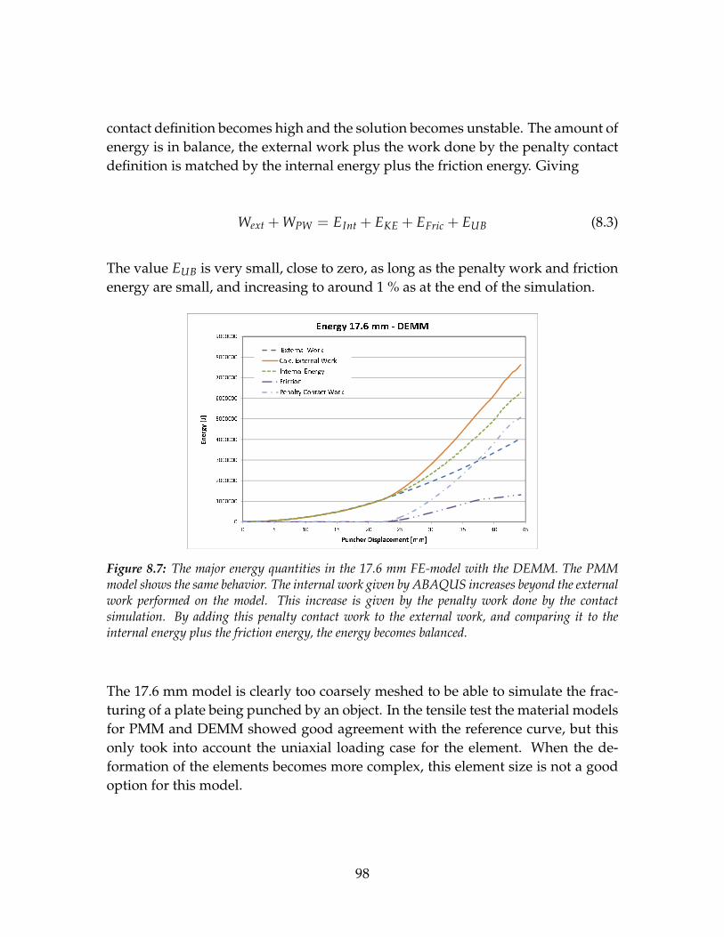
contact definition becomes high and the solution becomes unstable. The amount ofenergy is in balance, the external work plus the work done by the penalty contactdefinition is matched by the internal energy plus the friction energy. Giving

Wext + WPW = EInt + EKE + EFric + EUB (8.3)

The value EUB is very small, close to zero, as long as the penalty work and frictionenergy are small, and increasing to around 1 % as at the end of the simulation.

Figure 8.7: The major energy quantities in the 17.6 mm FE-model with the DEMM. The PMMmodel shows the same behavior. The internal work given by ABAQUS increases beyond the externalwork performed on the model. This increase is given by the penalty work done by the contactsimulation. By adding this penalty contact work to the external work, and comparing it to theinternal energy plus the friction energy, the energy becomes balanced.

The 17.6 mm model is clearly too coarsely meshed to be able to simulate the frac-turing of a plate being punched by an object. In the tensile test the material modelsfor PMM and DEMM showed good agreement with the reference curve, but thisonly took into account the uniaxial loading case for the element. When the de-formation of the elements becomes more complex, this element size is not a goodoption for this model.

98

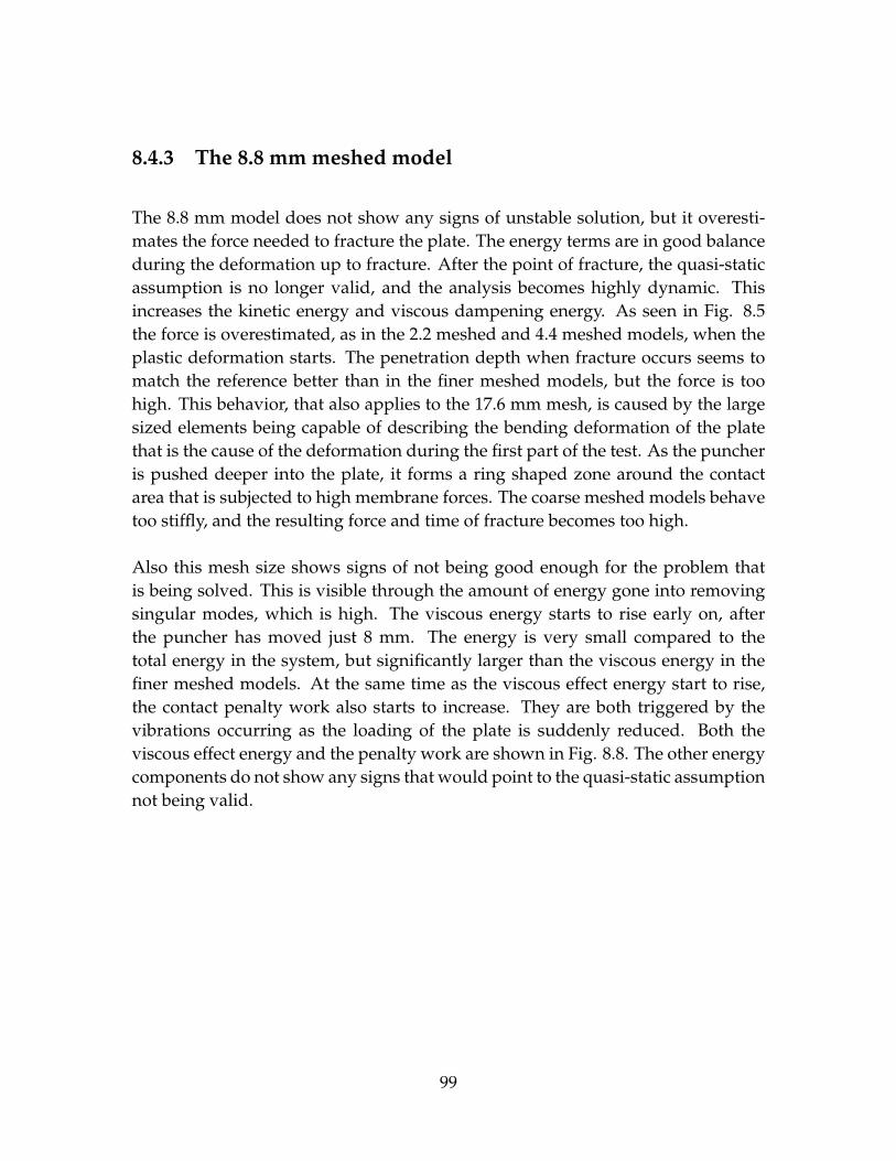
8.4.3 The 8.8 mm meshed model

The 8.8 mm model does not show any signs of unstable solution, but it overesti-mates the force needed to fracture the plate. The energy terms are in good balanceduring the deformation up to fracture. After the point of fracture, the quasi-staticassumption is no longer valid, and the analysis becomes highly dynamic. Thisincreases the kinetic energy and viscous dampening energy. As seen in Fig. 8.5the force is overestimated, as in the 2.2 meshed and 4.4 meshed models, when theplastic deformation starts. The penetration depth when fracture occurs seems tomatch the reference better than in the finer meshed models, but the force is toohigh. This behavior, that also applies to the 17.6 mm mesh, is caused by the largesized elements being capable of describing the bending deformation of the platethat is the cause of the deformation during the first part of the test. As the puncheris pushed deeper into the plate, it forms a ring shaped zone around the contactarea that is subjected to high membrane forces. The coarse meshed models behavetoo stiffly, and the resulting force and time of fracture becomes too high.

Also this mesh size shows signs of not being good enough for the problem thatis being solved. This is visible through the amount of energy gone into removingsingular modes, which is high. The viscous energy starts to rise early on, afterthe puncher has moved just 8 mm. The energy is very small compared to thetotal energy in the system, but significantly larger than the viscous energy in thefiner meshed models. At the same time as the viscous effect energy start to rise,the contact penalty work also starts to increase. They are both triggered by thevibrations occurring as the loading of the plate is suddenly reduced. Both theviscous effect energy and the penalty work are shown in Fig. 8.8. The other energycomponents do not show any signs that would point to the quasi-static assumptionnot being valid.

99

Figure 8.8: The energy going to viscous effects and the work done by the contact definition for the8.8 mm meshed model.

8.4.4 The 2.2 mm and the 4.4 mm meshed model

The 2.2 mm and 4.4 mm meshed model show good agreement with the referencecurve when it comes to the force needed to fracture the plate (Fig 8.5) The peakdifference for the two mesh sizes is the 4.4 mm PMM model that has a deviationof 5 % from the maximum force of the reference curve. The three other deviateby around 1 % higher maximum force. The fracture happens at a lower value ofpenetration for the puncher. For the 4.4 mm model, the DEMM FE-model rupturesbefore the PMM FE-model. This is because even if the tuning of the material isdone ever so thoroughly in the tensile test, there will always be a difference in thepoint of final fracture. The DEMM gives a higher value of penetration before thefailure occurs compared to the PMM, if their tensile test tuning shows an equalelongation at the point of fracture. This happens for the 2.2 mm meshed plate. Forthe 4.4 mm and 8.8 mm models the DEMM model has a slightly lower elongationat fracture in the tensile test, than the PMM for the same mesh size, as indicatedby the increase in damage dissipated energy in Fig. 7.15. This difference is em-phasized in the plate penetration test, giving a lower penetration value at fracturefor the DEMM than for the PMM. This effect is clearly enlarged when the mate-rial models are used on the plate puncture experiment. This can clearly be seenin the energy dissipated by damage for the 4.4 mm model, shown in Fig. 8.11. It

100

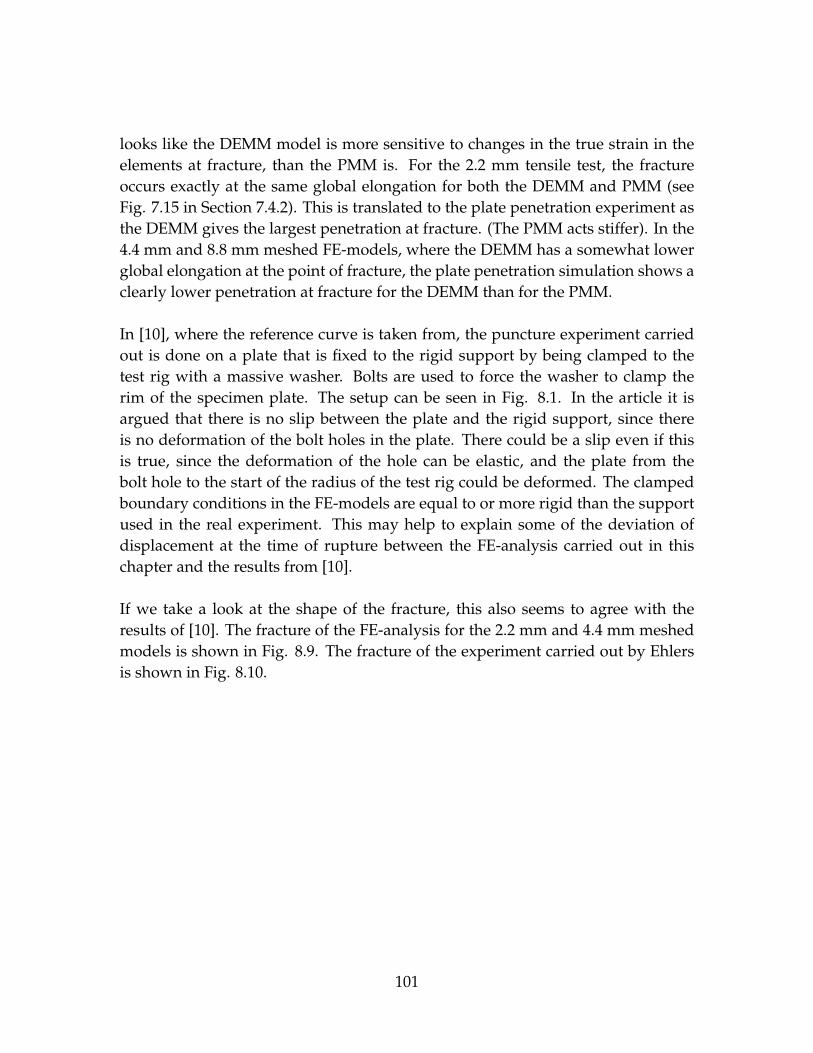
looks like the DEMM model is more sensitive to changes in the true strain in theelements at fracture, than the PMM is. For the 2.2 mm tensile test, the fractureoccurs exactly at the same global elongation for both the DEMM and PMM (seeFig. 7.15 in Section 7.4.2). This is translated to the plate penetration experiment asthe DEMM gives the largest penetration at fracture. (The PMM acts stiffer). In the4.4 mm and 8.8 mm meshed FE-models, where the DEMM has a somewhat lowerglobal elongation at the point of fracture, the plate penetration simulation shows aclearly lower penetration at fracture for the DEMM than for the PMM.

In [10], where the reference curve is taken from, the puncture experiment carriedout is done on a plate that is fixed to the rigid support by being clamped to thetest rig with a massive washer. Bolts are used to force the washer to clamp therim of the specimen plate. The setup can be seen in Fig. 8.1. In the article it isargued that there is no slip between the plate and the rigid support, since thereis no deformation of the bolt holes in the plate. There could be a slip even if thisis true, since the deformation of the hole can be elastic, and the plate from thebolt hole to the start of the radius of the test rig could be deformed. The clampedboundary conditions in the FE-models are equal to or more rigid than the supportused in the real experiment. This may help to explain some of the deviation ofdisplacement at the time of rupture between the FE-analysis carried out in thischapter and the results from [10].

If we take a look at the shape of the fracture, this also seems to agree with theresults of [10]. The fracture of the FE-analysis for the 2.2 mm and 4.4 mm meshedmodels is shown in Fig. 8.9. The fracture of the experiment carried out by Ehlersis shown in Fig. 8.10.

101

Viewport: 1 ODB: I:/MASTEROPPGAVE/TENSILE .../Penetration_2_2−DEMM.odb

XY

Z

Viewport: 2 ODB: I:/MASTEROPPGAVE/TENSILE ...e/Penetration_2_2−PMM.odb

XY

Z

Viewport: 3 ODB: I:/MASTEROPPGAVE/TENSILE .../Penetration_4_4−DEMM.odb

XY

Z

Viewport: 4 ODB: I:/MASTEROPPGAVE/TENSILE ...e/Penetration_4_4−PMM.odb

XY

Z

Figure 8.9: The shape of the fracture of the plate for the 2.2 mm and 4.4 mm meshed models, withboth PMM and DEMM. Top left: 2.2 mm with DEMM, Top Right: 2.2 mm model with PMM,Bottom left: 4.4 mm model with DEMM and Bottom right: 4.4 mm model with PMM.

Figure 8.10: The fracture shape of four different plate samples after the puncture test experiment.[10]

The shape of the fracture is similar to the real fracture for the 2.2 mm model. It has

102

enough elements to recreate the shape seen in Fig. 8.10. The 8.8 mm model doesnot have enough elements in the fracture zone to display the same rupture patternas the 2.2 mm model, but the basic shape can be seen. For both the different meshsizes, the PMM and the DEMM gives the same shape of the fracture.

The energy outputs for the 2.2 mm and the 4.4 mm models (Fig. 8.12 to 8.15)confirmthe quasi-static approach that is assumed up to the point of fracture. The externalwork is matched by the internal energy up to the point of fracture. From this pointand further, the structures respond dynamically because the load is suddenly re-moved. The DEMM model gives a higher amount of penalty contact energy com-pared to the PMM, but this is the only major difference between the major energyoutputs for the two material models. As in the tensile test, the amount of energyrecorded as going into dissipating damage is different because of the different ap-proaches in obtaining the damage. The differences are as expected after seeing theresults of the tensile test, and are very small compared to the amount of energypresent in the system. The energy difference in damage dissipated energy is seenin Fig. 8.11.

Figure 8.11: The damage dissipated energy for the 2.2 mm mesh plate (left) and the 4.4 mm meshedplate (right).

103

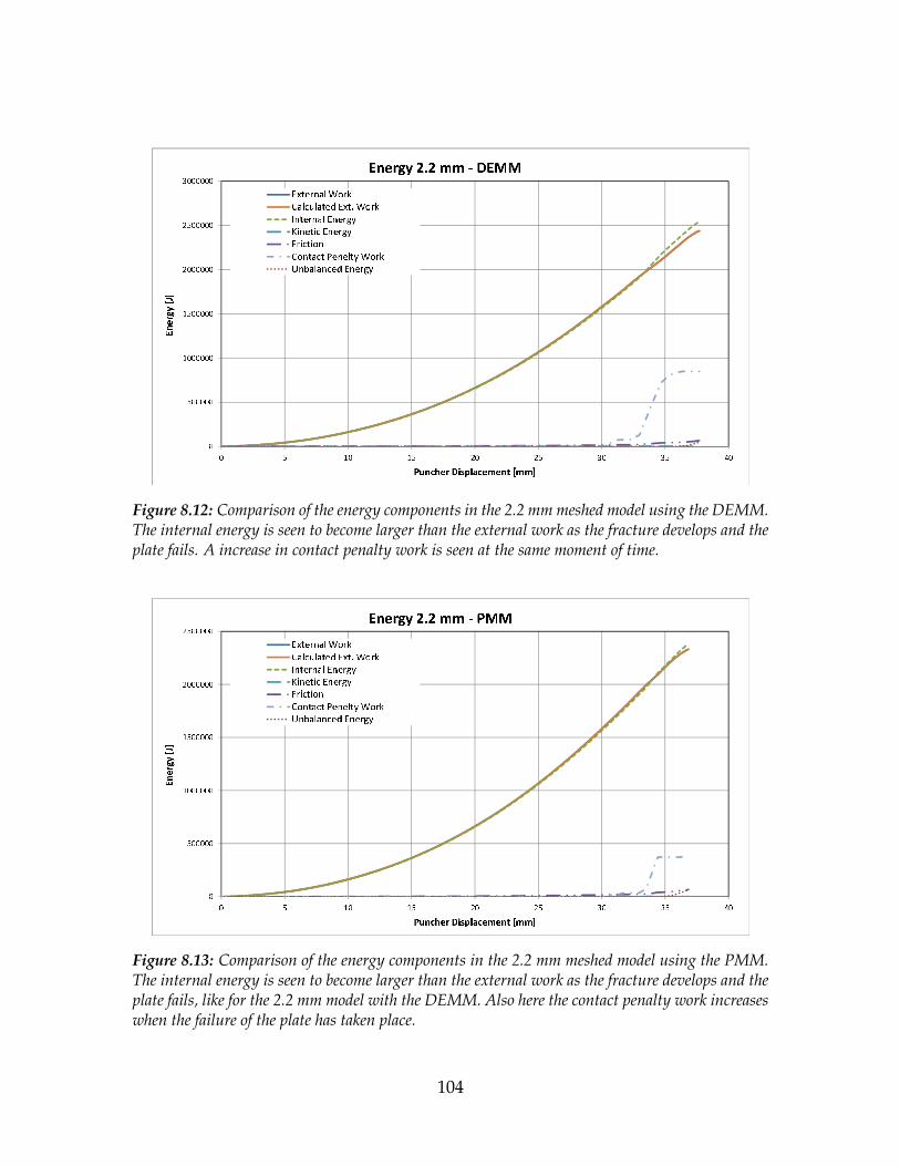
Figure 8.12: Comparison of the energy components in the 2.2 mm meshed model using the DEMM.The internal energy is seen to become larger than the external work as the fracture develops and theplate fails. A increase in contact penalty work is seen at the same moment of time.

Figure 8.13: Comparison of the energy components in the 2.2 mm meshed model using the PMM.The internal energy is seen to become larger than the external work as the fracture develops and theplate fails, like for the 2.2 mm model with the DEMM. Also here the contact penalty work increaseswhen the failure of the plate has taken place.

104

Figure 8.14: Comparison of the energy components in the 4.4 mm meshed model using the DEMM.The internal energy is equal to or smaller than the external work, and the other energy componentsare small during the whole simulation.

Figure 8.15: Comparison of the energy components in the 4.4 mm meshed model using the PMM.Like for the 4.4 mm DEMM model, the internal energy is equal to or smaller than the external work,and the other energy components are small during the whole simulation.

105

8.4.5 Reduction of structural strength

As expected after performing the tensile test, the remaining strength of the mate-rial involved in the fracture varies significantly between the two material modelsused for each mesh size. In Fig. 8.16, the difference in damage done to the ele-ments involved in the fracture of the plate are shown for the 2.2 mm mesh. Thered elements are elements that have gotten their stiffness reduced to zero, andwhich are deleted. The blue elements are elements that have gotten their stiffnessreduced and will have a lower load-bearing capacity if the structure would havebeen applied a new load.

Viewport: 2 ODB: I:/MASTEROPPGAVE/TENSILE ...e/Penetration_2_2−PMM.odb

XY

Z

Viewport: 4 ODB: I:/MASTEROPPGAVE/TENSILE ...e/Penetration_4_4−PMM.odb

XY

Z

Viewport: 3 ODB: I:/MASTEROPPGAVE/TENSILE .../Penetration_4_4−DEMM.odb

XY

Z

Viewport: 1 ODB: I:/MASTEROPPGAVE/TENSILE .../Penetration_2_2−DEMM.odb

XY

Z

Figure 8.16: The figure shows the elements that have gotten their elastic stiffness reduced by thefracture models. The DEMM applies damage to more elements than the PMM, and the overallstrength of the material in the zone of fracture is therefore reduced more. Top left: 2.2 mm DEMM,Top right: 2.2 mm PMM, Bottom left: 4.4 mm DEMM and Bottom Right: 4.4 mm PMM.

As explained in Section 7.4.3, this does not influence the results of these experi-ments, since the reduced stiffness is used to simulate the fracture directly. If, on theother hand, the plate simulated in this chapter would have to be reloaded again,

106

the reduced stiffness of the elements around the hole in the DEMM created by thefracture would give a weaker zone than in the PMM model. The structures usingthe different material models could then have behaved quite differently from eachother.

107

Chapter 9

Summary and conclusion

In this thesis the theory of ductile fracturing of ductile materials simulated usingthe finite element method is studied. The material behavior during a fracture isexplained on a microscopic level, and different theories on how to describe thegrowth and coalition of material voids is explained. This includes models describ-ing the formations of void in a continuous homogeneous material developed byA.S. Argon et al., and models to describe the growth and coalition of voids devel-oped by Rice and Tracey [21] and Gurson [12].

In the finite element method, the approach taken is somewhat different. A methoddeveloped by Sören Ehler and Petri Varsta [11] makes use of the material input ina FE-analysis to tune the material’s plastic properties into being able to describethe localized effect of instability caused by the ductile fracture. Their method iscompared to a fracture model that is already in use in the FE-analysis softwarepackage ABAQUS, developed by Hillerborg et al. [17]. This model defines thefracture of the FE-model by the energy needed to open a unit area of crack.

In the method developed by Hillerborg et al., a fracture displacement measure uplf

is used to define the elongation of the element from damage initiation to fracture.The model presented defines this as being equal to the global elongation for themodel during the simulated creation of the crack. This is true only if there is justone element in the direction of elongation that is influenced by the fracture model.If more than one element in the direction of elongation is influenced by the fracturemodel, the resulting fracture displacement becomes larger than the value of upl

f in-

108

putted in the material definition. This affects the assumed mesh independence ofthis material model, since differently sized elements will behave differently. Thisbehavior of multiple elements contributing to the fracture displacement can be re-duced by including a more specified damage initiation criterion, involving param-eters such as the stress triaxiality and the lode parameter, to better control whichelements are included in the fracture model.

By using a tensile test experiment as reference, the two fracture models were tunedto give the same global response regarding the force-displacement of a tensiletest piece simulated using ABAQUS. The two material models, referred to as thePlasticity-material-model (PMM) for the method given by Ehlers and Varsta, andthe Damage-Evolution-model (DEMM) for the method developed by Hillerborg etal., showed good agreement with each other when simulating the tensile fractureof the tensile specimen using a quasi-static approach. The simulations were per-formed using as large element sizes as possible, considering the application lateron. The energy terms did not differ for any of the mesh sizes used with the twomaterial models. One difference that was found between using the two methods todescribe the fracture behavior is the damaging of the material inside the unstablezone when using the DEMM. This results in a zone of weaker elements around thefracture developed, that will influence the residual strength of the FE-model. Thisbehavior of reduced strength due to the fracturing process is not present whenusing the PMM.

The material models developed for the different mesh sized dog-bone tensile mod-els were then used as the material input in a simulation of a circular steel platebeing punctured by a cone-shaped puncher. The simulation was performed us-ing a constant speed to force the puncher through the plate. The two models thatused the largest element sizes of 17.6 mm and 8.8 mm in side length, showed signsof being too coarsely meshed for the problem that was being solved. The twofiner meshed models gave the right value of force needed to fracture the plate,but the fracture occurred prematurely compared to the reference. This was prob-ably caused by the boundary conditions giving a stiffer behavior compared to thereference experiment. The DEMM and PMM showed almost perfect behavior re-garding the global force and displacement relationship in the tensile test.

In the tensile test experiment, the element size did not matter much, since the ma-terial models could be set to give the right global response regarding the uniaxialload case for all the models regardless of the size of the elements. When the de-

109

formation is more focused on the bending behavior of the element, the elementsize compared to the global size of the modeled plate is more critical. The coarsermeshed models of 8.8 mm and 17.6 mm did show signs of having too few ele-ments to simulate the real world behavior. As long as the problem was dominatedby bending the response match the finer meshed models, but as the penetrationof the puncher started to deform the plate in such a way that in-plane membraneforces began to dominate the fracture behavior, the coarser meshed models begunto behave too stiffly compared to the finer meshed 2.2 mm and 4.4 mm models.

Looking at the energy components, no significant differences between the two ma-terial models cannot be found before the final fracture occurs. Up to this point,the kinetic energy, viscous dampening energy, contact dissipated energy and "ar-tificial" strain energy are small, if not zero. When the fracture develops and theforce applied is suddenly reduced, this introduces dynamic effects that make thementioned energy parameters rise and become different for the two models.

In the penetration experiment, the small difference in global behavior from thetensile test becomes larger, and influences the result by giving a clearly larger pen-etration depth for one of the material models compared to the other. The elementdamage effect caused by the accumulation of damage seems to give the modelsthat utilize the DEMM a softer behavior than the model using the PMM, in theplate penetration test. This occurred if the material models gave exactly the sameresult in the tensile test. This effect is explained by the softening of the elements inthe model using the DEMM, giving a softer transition from the unstable behaviorof necking to final fracture, and resulting in a smaller applied force at the time offinal failure. In a collision event simulation, where the striking object is often set tohave an initial kinetic energy that is transferred to the stuck object, the differenceof damage accumulation may yield some greater differences in the response of thedeformable structure.

110

Appendix A

Appendix A

In this appendix, the model for plasticity and damage and failure for ductile metalsin ABAQUS is presented as it is being used by the software program.

A.1 Material Plasticity in Abaqus

In ABAQUS, a material model for ductile materials is used for the calculations ofthe plastic behavior of the material. This model can be used on rate-independentand rate-dependent materials, and has simple algebraic equations with a stiffnessmatrix that can be explicitly developed. This makes it fast and easy to use. Theinput data is inputted as a true equivalent stress to true equivalent plastic strain re-lationship, and the first line must contain a stress-strain state with zero equivalentplastic strain. This data point is used to calculate the yielding of the material 1. Theinputted data must be arranged in increasing order depending on the equivalentstress, otherwise ABAQUS will abort the analysis and display an error message.

The plasticity of a material is assumed to be governing the deformation when thevon Mises yield criterion is satisfied. This criterion is given as ([7] sec. 4.3.2.)

1The yielding point is the transition between a pure elastic behavior and an elasto-plastic mate-rial, according to the von Mises yield criteria.

111

(a) The input menu for the plas-tic properties in a material. Fora rate-independent material only thetrue stress and the true strain areinputted, additionally there can beadded temperature- and strain ratedependent data and different fieldvariables. Different suboptions canalso be assigned.

(b) The inputted data in figure A.1(a) willproduce a true stress-true strain relationshipas shown here. After the last point of in-putted data, ABAQUS assumes that the ma-terial will behave perfectly plastically, givingthe straight line.

q = σ(epl) (A.1)

For rate-independent materials σ = σ0, and for rate dependent materials, the plas-ticity is dependent on the temperature- and the strain rate.

At the end of each increment, the criterion is tested against the fully elastic be-havior, and if the equivalent stress in the material satisfies the criterion, the plasticbehavior is used in the next increment in order to calculate the stress and strain.

As the material follows the plastic behavior of the model, the incremental stressand strain relation is defined as

∂σ =

[Qζ + (K− 1

3Q)I I − RSS

]: ∂ε (A.2)

where

112

Q =23

q23

√e : e

(A.3)

S =2 E

2(1−ν)

1 +3 E

2(1−ν)q ∆epl

e (A.4)

R =1qe

1− ∆epl dσdepl /q

1 + dσdepl /

3E2(1−ν)

(A.5)

,

I is the identity matrix and ζ is the fourth-order unit tensor. This definition is validfor bodies where there are three direct strains defined by the kinematic solution. Ifthere is a state of plane stress or uniaxial stress, the relation is somewhat simpler.For plane stress, the incremental stress and strain relation is found by imposing thecondition of ∂σ33 = 0 into equation (A.2). For uniaxial stress the relation is simplythe direct variation of σ11 = 2/3S11, that is

∂σ11 =

[32

Q− Rσ211

]∂ε11 (A.6)

A.2 Damage Initiation Criteria

ABAQUS offers a wide range of different models in order to define the point offailure initiation and the following damage evolution. For isotropic ductile mate-rials, the Damage Initiation criterion for fracture of metals is used. This criterion usesthe true stress and true strain state in the element to evaluate if the element satis-fies the criterion inputted by the user. For ductile fracture, three damage initiationcriteria are provided; ductile criteria, shear criteria and Johnson-Cook criteria. Onlythe two first will be presented here. They are based on the model deveoped byHooputra et al. [18].

113

A.2.1 Ductile criteria

The ductile criterion is used to predict the onset of damage for a material due tonucleation, growth and coalescence of voids inside the material. The criterion ismet if the equivalent true strain in the element reaches a preset value, the equiva-lent true plastic strain at the onset of damage εpl

D . This preset value is dependenton the stress triaxiality η and the equivalent plastic strain rate ˙εpl in the element.([7] sec. 20.2.2)

εplD (η, ˙εpl) (A.7)

The evaluation of this criterion is done by comparing the incremental increase inequivalent plastic strain against the preset criterion for the state of stress triaxialityand strain rate the element is being deformed under. This is defined as

ωD =∫ dεpl

εplD (η, ˙εpl)

= 1 (A.8)

For each increment, the value ofωD will increase as

∆ωD =∆εpl

εplD (η, ˙εpl)

≥ 0 (A.9)

E.g. a material has defined a value for εplD in both tensile (positive strain rate)

and in compression (negative strain rate), and εplD,Ten = 2εpl

D,Comp. This means thatthe equivalent plastic strain for damage initiation for tensile loading is twice thatof compressive loading. If the material is first stretched to an equivalent plasticstrain value of 1

2εplD,Ten, the accumulated value of ωD will be 0.5. If the material

is then compressed, the material will reach the point of damage initiation whenthe compressive strain value is 1

2εplD,Comp, since this amount of compression will

also accumulate a value of ωD = 0.5. The tensile stretching of the material hasweakened it so that it can only withstand a fraction of the compressive load itwould have withstood without the initial stretching. This means that equation A.9

114

can also be written as

∆ωD =j

∑i=1

∆εpl

εplD , i(η, ˙εpl)

≥ 0 (A.10)

where j is the number of damage initiation criteria for different stress triaxialityand strain rate states that is used.

A.2.2 Shear criterion

The shear fracture damage initiation criteria works exactly the same way as theductile criterion, the only difference is that instead of stress triaxiality η, the stressstate is given by a shear stress ratioθS. This ratio is defined asθS = (q+ kS p)/τmax,where q is the von Mises stress, p is the hydrostatic stress, τmax is the maximumshear stress and kS is a material parameter. Following is the definition of the equiv-alent plastic shear stress at shear damage initiation εpl

S , and the shear initiationfactorωS.

εplS (θS, ˙εpl) (A.11)

ωS =∫ dεpl

εplS (θS, ˙εpl)

= 1 (A.12)

∆ωS =∆εpl

εplS (θS, ˙εpl)

≥ 0 (A.13)

A.3 Damage evolution

When an element has met the damage initiation criterion (e.x. ωD = 1), a damageevolution can be found for which the true stress is reduced to zero when the true

115

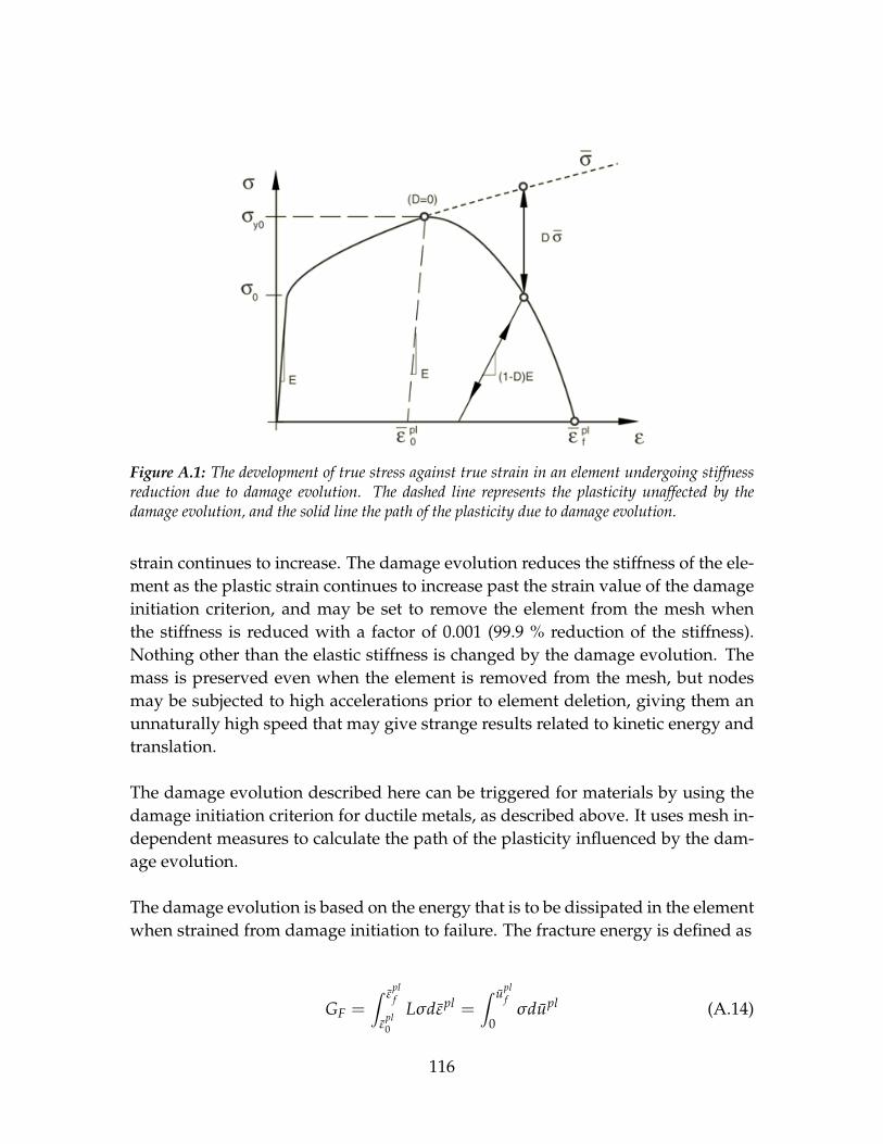
Figure A.1: The development of true stress against true strain in an element undergoing stiffnessreduction due to damage evolution. The dashed line represents the plasticity unaffected by thedamage evolution, and the solid line the path of the plasticity due to damage evolution.

strain continues to increase. The damage evolution reduces the stiffness of the ele-ment as the plastic strain continues to increase past the strain value of the damageinitiation criterion, and may be set to remove the element from the mesh whenthe stiffness is reduced with a factor of 0.001 (99.9 % reduction of the stiffness).Nothing other than the elastic stiffness is changed by the damage evolution. Themass is preserved even when the element is removed from the mesh, but nodesmay be subjected to high accelerations prior to element deletion, giving them anunnaturally high speed that may give strange results related to kinetic energy andtranslation.

The damage evolution described here can be triggered for materials by using thedamage initiation criterion for ductile metals, as described above. It uses mesh in-dependent measures to calculate the path of the plasticity influenced by the dam-age evolution.

The damage evolution is based on the energy that is to be dissipated in the elementwhen strained from damage initiation to failure. The fracture energy is defined as

GF =∫ εpl

f

εpl0

Lσdεpl =∫ upl

f

0σdupl (A.14)

116

where σ is the equivalent true stress in the element.

The damage evolution is defined as mesh independent because it does not directlyuse any parameters that are dependent on the element size in the model. Insteadof defining the deformation after damage initiation as plastic strain, it is definedas an equivalent plastic displacement upl. It is defined as

˙upl = L ˙εpl (A.15)

where L is a characteristic element length calculated from the initial geometry of theelement. (See section 4.4.2 for further details.)

At the point of damage initiation, the overall damage variable D is zero, as seen inFig. A.1. As the element is deformed and the strain value increases, D will increasein value reducing the elastic stiffness of the element to (1−D)E. The true stress inthe element σ is also reduced from its undamaged value (the dashed line in figureA.1) to the value of σ = Dσ . At the point of damage initiation, the stress is σy0,

the plastic strain is εpl0 and D = 0. At the point of failure and element deletion the

stress is zero, the plastic strain is εplf and D = 1. The path between these two points

can be defined by the physical deformation as a straight line, a curve defined byseveral points defined by a value of D and a corresponding deformation measure,or exponential. Alternatively it can be defined as the amount of energy that willbe dissipated during the deformation from damage initiation to failure, either in alinear or exponential form.

For each damage initiation criterion, there may be a contribution to the overalldamage of the material in the element. Therefore an overall damage variable D iscalculated as

D = max{

dmult, max j∈Nmax(d j)}

(A.16)

where d is an individual damage evolution damage variable and dmult is a com-bination of two or more independent damage evolutions with different damageinitiation criteria.

117

1

0

d

U^plU^pl

1

0

d

Uf^plU^pl

1

0

d

Uf^pla: Tabular b: linear c: exponential

Ufpl

Upl Upl Upl

Ufpl Uf

pl

Figure A.2: When using the Upl to define the damage evolution, there path of the elements truestress/true strain relationship can be define in three difrrenet ways.The linear model follows astraight line from damage initiation to failure, while the tabular option allows the definition ofpoints defined by the damage parameter D and the damage elongation length upl . The exponentialoption is defined by an endpoint as in the linear option, and a parameter regulating the amount ofcurvation of the path.

dmult = 1− ∏k∈Nmult

(1− dk) (A.17)

Nmult and Nmax are the sets of active mechanisms that contribute to the overalldamage in a multiplicative and a maximum sense.

If an element undergoing deformation in the damage evolution domain is un-loaded, it will follow a linear unloading path defined by the current elastic stiffnessin the element. Later, when a new load is applied, it will follow the same elasticpath back to the path defined by the damage evolution, and continue the plasticdeformation according to this.

It is worth noting that the damage initiation and damage evolution is used in eachintegration point in the element independently. This means that a solid elementwith one integration point will only be evaluated in that point altogether. A shellelement with multiple integration points through the thickness of the element, willevaluate the damage initiation and damage evolution differently for each of theintegrations point. For pure compression and pure tensile loading, this will notinfluence the behavior, but for bending, the different integration points will fail atdifferent plastic strains because of the different loading pattern for each of them.

118

Bibliography

[1] Ansi/ieee std 754-2008, ieee standard for binary floating-point arithmetc.Technical Report 754-2008, IEEE, 2008.

[2] T. L. Anderson. Fracture Mechanics - Fundamentals and Applications - Third Edi-tion. taylor & Francis, 2008.

[3] Yuanli Bai and Tomasz Wierzbicki. A new model of metal plasticity and frac-ture with pressure and lode dependence. International Journal of Plasticity,24(6):1071–1096, 2008.

[4] I. Barsoum, J. Faleskog, and S. Pingle. The influence of the lode parameter onductile failure strain in steel. Procedia Engineering 10, 10:69–75, 2011.

[5] Shailendra Singh Bhadauria, M.S. Hora, and K.K. Pathak. Effect pf stresstriaxiality on yielding of anisotropic materials under plane stress condition.Journal of Solid Mechanics, 1(3):226–232, 2009.

[6] Robert D. Cook, David S. Malkus, Michael E. Plesha, and Robert J. Witt. Con-cepts and Applications of Finite Element Analysis. John Wiley & Sons, 2007.

[7] Dassault Systémes. Abaqus Analysis User’s Manual, ver. 6.11 edition.

[8] Dassault Systémes. Abaqus/CAE User’s Manual, ver. 6.11 edition.

[9] Dassault Systémes. Getting started with Abaqus: Interactive Edition, ver. 6.11edition.

[10] Sören Elhers. Strain and stress relation until fracture for finite element simu-lations of a thin circular plate. Thin-Walled Structures 48, 48(1):1–8, 2010.

[11] Sören Elhers and Petri Varsta. Strain and stress relation for non-linear finiteelement simulations. Thin-Walled Structures 47, 47(11):1203–1217, 2009.

119

[12] A.L. Gurson. Continuum theory of ductile rupture by void nucleation andgrowth: Part i - yield criteria and flow rules of porous ductile media. Journalof Engineering Materials and Technology, 99:2–15, 1977.

[13] Tor Erik Hals. Konstruksjonsmekanikk. Tapis Forlag, 2 edition, 1999.

[14] R. Hill. The Mathematical Theroy of Plasticity. Oxford University Press Inc.,oxford classical (published 1998) edition, 1950.

[15] A. Hillerborg. A model for fracture analysis. Technical report, Division ofbuilding materials the Lund Institute of Technology, 1978.

[16] A. Hillerborg. The theoretical basis of a method to determine the fractureenergy gf of concrete. Materials and Structures, 18:291–296, 1985.

[17] A. Hillerborg, M. Modéer, and P.E. Petersson. Analysis of crack formation andcrack growth in concrete by means of fracture mechanics and finite elements.Cement and Concrete Research, 6(6):773 – 781, 1976.

[18] H Hooputra, H Gese, H Dell, and H Werner. A comprehensive failure modelfor crashworthiness simulation of aluminium extrusions. International Journalof Crashworthiness, 9(5):449–464, 2004.

[19] Jay R. Lund and Joseph P. Byrne. Leonardo da vinci’s tensile strength tests:Implications for the discovery of engineering mechanics. Civil Engineering andEnvironmental Systems, 18(3):243–250, 2001.

[20] J. Oliver. A consistent characteristic length for smeared cracking models. In-ternational Journal for Numerical Methods in Engineering, 28(2):461–474, 1989.

[21] J.R. Rice and D.M. Tracey. On the ductile enlargement of voids in triaxialstress fields. Journal of the Mechanics and Physics of Solids, 17(3):201–217, 1969.

[22] Viggo Tvergaard. On localization in ductile materials containing sphericalvoids. International journal of fracture, 18(4):237–252, 1982.

[23] Viggo Tvergaard. Material failure by void growth to coalescence. Advances inApplied Mechanics, 27:83–151, 1989.

[24] Tomasz Wierzbicki and Norman Jones. Structural failure. John Wiley and SonsInc., 1989.

120

121