Simulating complex tumor dynamics from avascular to vascular growth

using a general level-set method

Cosmina S. Hogeaa, Bruce T. Murraya, James A. Sethianb

aDepartment of Mechanical Engineering, Binghamton University, Binghamton, NY 13902, USA bDepartment of Mathematics and Lawrence Berkeley National Laboratory, University of California, Berkeley, CA 94721, USA * This author was supported in part by the Applied Mathematical Sciences subprogram of the Office of Energy Research, U.S. Department of Energy, under Contract Number DE-AC03-76SF00098, and the Division of Mathematical Sciences of the National Science Foundation

Abstract

A comprehensive continuum model of solid tumor evolution and development is

investigated in detail numerically, both under the assumption of spherical symmetry and

for arbitrary two-dimensional growth. To our knowledge, this is the first investigation of

the multicell model developed by De Angelis and Preziosi (2000) as a moving boundary

problem in higher dimensions and arbitrary geometries. The model represents both the

avascular and the vascular phase of tumor evolution, and is able to simulate when the

transition occurs; progressive formation of a necrotic core and a rim structure in the

tumor during the avascular phase are also captured. In terms of transport processes, the

interaction of the tumor with the surrounding tissue is realistically incorporated. A

computational framework, based on a Cartesian mesh/narrow band level-set method, has

been developed in order to solve the coupled advection-diffusion model equations with a

moving boundary inside a fixed domain. The solution algorithm is designed so that

extension to three-dimensional simulations is straightforward.

Keywords: multicell model, avascular, vascular, tumor angiogenic factor, angiogenesis,

vascularization, necrotic core, level set method, narrow band, finite differences

1

1. Introduction

Over the last ten years, a number of important advancements have been made in the

development of mathematical models to simulate the growth and macroscopic behavior

of solid malignant tumors. The recent reviews by Araujo and McElwain [5] and Bellomo,

et al. [6] contain extensive bibliographies and categorize the different solid tumor growth

models. As in many areas of fundamental and applied science, the increasing

sophistication of computational models make them an important part of the study of

complex multi-scale phenomena. Verifiable computational models will likely become

part of the arsenal of techniques used to better understand tumor evolution and treatment

strategies in the near future. Continuum-based models can be used to help predict the

evolution of a tumor's boundary in time and this knowledge may in turn help estimate the

effect that various methods of treatment (e.g., chemotherapy, ultrasound) may have on

the tumor behavior as well as on the surrounding healthy tissue and, ultimately, on the

host.

Malignant solid tumors are masses of tissue formed as a result of abnormal and

excessive proliferation of mutant (atypical) cells, whose division has escaped the

mechanisms that control normal cellular proliferation. This abnormal proliferation of

atypical cells can lead to uncontrolled growth, if not checked by the immune system. In

simple terms, tumor growth (spread of malignant cells) can be described as follows: when

fed with a sufficient amount of nutrient, malignant cells divide (cellular mitosis); when

the density of cells in a specific volume becomes high, the cells are compressed by their

neighbors and tend to move to less populated areas–where they may continue to

2

proliferate–and this process is repeated. The growing tumor mass eventually begins to

interact with the surrounding tissue and may eventually evolve in a complex manner.

There are different stages of a malignant tumor evolution; described roughly, the main

stages are the cellular stage and the macroscopic stage. The cellular stage refers to the

early stage of a tumor evolution, when proliferating tumor cells have not begun to

agglomerate. The macroscopic stage comes about when clusters of atypical cells

condense together into a compact shape (e.g., spherical); this stage is sub-divided into

two subsequent phases−the avascular phase and the vascular phase. During the avascular

phase, the tumor obtains nutrients via diffusion processes alone from the local

environment. In the second phase, called the vascular phase, the tumor attempts to

develop its own blood supply through the process of angiogenesis (i.e., the birth of new

blood vessels). Malignant tumor cells secrete chemicals that diffuse outward into the

surrounding healthy tissue and stimulate the growth of new capillary blood vessels; the

newly formed blood vessels penetrate into the tumor mass feeding it with nutrients and

leading to a rapid growth of the tumor (Folkman, [16]).

Due to the extremely complex nature of the biological systems underlying the behavior

in tumors and to the limited understanding of tumor growth mechanisms, developing

realistic models (mathematical, computational or both) is a difficult task. Currently, there

are two major approaches for solid tumor growth modeling: the first employs continuum

models to describe the evolution of the tumor in terms of systems of partial differential

equations and/or non-linear integro-differential equations; the second approach uses

discrete lattice or Cellular Automata (CA) models (e.g., Kansal, et al., [19]; Mansury and

Diesboeck, [24]). For the macroscopic stage of tumor evolution, the continuum approach

3

may offer the most generality. Assuming that all of the model parameters can be

estimated, the advantage of a continuum model is that it provides a systematic means for

evaluating the role played by individual physical mechanisms. However, the more

complex the continuum model−the more difficult the computational simulations, since a

continuum model will generally yield a nonlinear moving boundary problem described

by systems of partial differential equations. The starting point for many continuum

models is the pioneering work of Greenspan in the 1970's (see Araujo and McElwain, [5]

and references therein). In recent years a variety of macroscopic continuum models have

been derived employing analogies with inorganic systems (theory of mixtures,

multiphase flow, e.g., Byrne, et al. [8] or Byrne and Preziosi [9]). While currently quite a

few such complex models exist in the literature, computational simulations in arbitrary

geometries and higher dimensions to further investigate and validate these models are

still largely missing. Only very recently, such calculations have started to emerge

[14],[40].

The goal of the present work is to investigate a recent comprehensive model

DeAngelis and Preziosi (2000) [15], which involves multiple cell populations as well as

chemical species. From a mathematical/computational point of view, the model is

complex since it consists of a system of five PDEs, with some of the field variables as

well as some of the coefficients discontinuous across the tumor boundary; the tumor

surface evolves in time, and its location must be determined as part of the solution. At the

same time, from a biological point of view, this model is very appealing for the following

reasons: first of all, it captures both the avascular and the vascular stages of tumor growth

(based on nutrient levels, the model predicts evolution from the avascular phase into the

4

vascular one); second, it incorporates the interaction of the tumor with the surrounding

environment (primarily in terms of the angiogenesis phenomenon); third, effects of

potential treatments on the tumor evolution can be readily investigated by varying the

model parameters.

A general computational framework for obtaining multi-dimensional solutions to

continuum-based models for numerically simulating tumor growth has been developed

and is described in Hogea, et al. [17]. In that work, the solution methodology is tested on

a simplified, two-equation model. Finite-differences on a fixed Cartesian grid are

employed to discretize the field equations, and the level set method is used to determine

the location of the evolving tumor boundary. Here, the methodology is applied to the

complex model involving coupled nonlinear reaction/advection/diffusion equations [15]

in a two-region domain with an evolving tumor boundary.

The structure of the paper is as follows: Section 2 reviews the mathematical tumor

growth model developed in DeAngelis and Preziosi [15]; Section 3 provides a brief

description of the general formulation of the level set method; Section 4 investigates the

spherically symmetric case –both from a biological and a computational point of view; a

comparison of the tumor evolution in time simulated via two different numerical methods

(a pseudo-Lagrangian and a level set – Eulerian one respectively) is performed; Section 5

presents the numerical algorithms for higher dimensions and arbitrary geometries;

Section 6 contains two-dimensional simulations of tumor evolution in arbitrary

geometries and various case scenarios for the model considered here; finally, Section 7

contains some remarks regarding further research.

5

2. Tumor growth model description

De Angelis and Preziosi [15] present a detailed derivation of the mathematical model

under investigation here. The model is summarized below. A slightly modified version is

reconsidered in Chaplain and Preziosi [11]. Geometrically, there are two regions in the

model: the inner region occupied by the tumor mass is time-dependent and denoted by

; the tumor region is embedded in a larger fixed domain denoted by D. The region

is referred to as the (tumor) outer environment.

)(tΩ

)()( tDtout Ω−=Ω

There are two classes of model dependent variables characterizing the physical state

of the biological system (i.e., in both the tumor mass and the outer environment): cell

populations and chemical species (macro-molecules). They are essentially different: the

cell size is much larger than that of the macro-molecules; the cells are delimited by a

membrane and can not penetrate each other; they occupy actual physical space. By

contrast, the chemical species consist of macro-molecules that may diffuse in the

intercellular space, attach to the cell membrane or penetrate it, such that they actually do

not take up physical space.

The following cell populations and chemical species are defined:

• living tumor cells – represented by the density ),( txuu TTr

=

• dead tumor cells – represented by the density ),( txuu DDr

=

• new capillaries (i.e., endothelial cells) with density ),( txuu CCr

=

• nutrient concentration ),( txuu NNr

=

• tumor angiogenic factor (TAF) concentration ),( txuu AAr

=

6

In a continuum mechanics framework, a standard mass balance law leads to a general

reaction-advection-diffusion equation for each of the model variables introduced above:

)()()()( uLuuWuQtu

−Γ+•∇−∇•∇=∂∂ r

(2.1)

where:

• is the generation (proliferation/production) term; )(uΓ=Γ

• is the death/decay term; )(uLL =

• is the drift velocity field; Wr

• is the diffusion coefficient. Q

The following modeling assumptions are made (from a biological viewpoint) in order to

specify the exact form of Eq.(2.1) for each of the continuum model field variables:

I. Regarding the tumor cells (living and dead)

1. living tumor cells proliferate (cellular mitosis) only if the levels of nutrient reaching

them are sufficient (i.e., above a certain threshold denoted by Nu~ );

2. living tumor cells die if the levels of nutrient reaching them are too low (i.e., below

the threshold denoted by Nu );

3. once a number of living cells inside the tumor have died due to insufficient

nutrient, the nutrient becomes sufficient for the remaining ones to survive; thus,

there is a smooth transition to a necrotic region;

7

4. when crowded by their neighbors, the living tumor cells have the ability to migrate

towards lower density areas where they have higher chances of surviving and

proliferating;

5. dead tumor cells do not move;

6. dead tumor cells are assumed to naturally disintegrate into waste products (water).

II. Regarding the tumor angiogenic factor (TAF)

1. living tumor cells are constantly producing TAF from a point on (in the revised

version, the assumption is made that living tumor cells produce TAF only when

they lack nutrient – i.e., haptotaxis occurs);

2. TAF diffuses both inside the tumor region and outside in the surrounding

environment;

3. TAF naturally degrades

III. Regarding the new capillaries

1. endothelial cells reached by TAF are stimulated to proliferate (cellular mitosis) at a

rate proportional to the concentration of TAF; proliferation decreases with the

density of new capillaries; in particular, proliferation stops if the density of the new

capillaries becomes higher than a certain threshold – here denoted by Cu ; the

endothelial cells first stimulated are those belonging to the pre-existing capillary

network, )(ˆˆ xuu CCr

= , in the tumor outer environment (the spatial distribution is

prescribed initially in the model and is assumed time-independent);

8

2. new endothelial cells undergo both a random motion (diffusion) and an ordered one

(chemotaxis) oriented towards the source of angiogenic stimulus (TAF) with

formation of new capillary sprouts by accumulation of endothelial cells;

3. newly formed endothelial cells undergo apoptosis.

IV. Regarding the nutrient:

1. the nutrient in the tumor outer environment is provided by the capillary network at a

linear rate; in particular, in the absence of new capillaries, the amount of nutrient in

the tumor outer environment is constant;

2. diffusion of nutrient inside the tumor is promoted by the presence of capillaries,

with the diffusion coefficient assumed to increase linearly with the density of

capillaries;

3. nutrient is consumed by the living tumor cells.

The model assumes that all cells (living cells, dead cells and endothelial cells) equally

contribute the overall cell density defined as:

(2.2) CCDT uuuuu ˆ+++=

It is assumed that there is a threshold overall cell density – here denoted by u and called

the close packing density (by analogy with multiphase flow terminology) – characterizing

the fact that no pressure is felt by a cell when the total density u is equal to it (i.e. the

stress vanishes for uu = ).

All the above modeling assumptions are placed in the context of the general advection-

diffusion equation (2.1) for each of the field variables (densities or concentrations). For

9

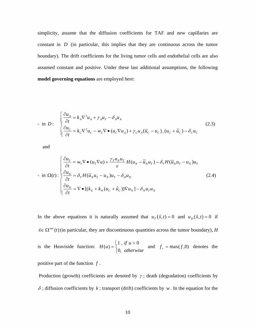
simplicity, assume that the diffusion coefficients for TAF and new capillaries are

constant in (in particular, this implies that they are continuous across the tumor

boundary). The drift coefficients for the living tumor cells and endothelial cells are also

assumed constant and positive. Under these last additional assumptions, the following

model governing equations are employed here:

D

- in : D

⎪⎪⎩

⎪⎪⎨

⎧

−+−+∇•∇−∇=∂

∂

−+∇=∂

∂

+ CCCCCCACACCCCC

AATAAAA

uuuuuuuuwukt

u

uuukt

u

δγ

δγ

)ˆ()()(2

2

(2.3)

and

- in : )(tΩ

⎪⎪⎪

⎩

⎪⎪⎪

⎨

⎧

−∇++•∇=∂

∂

−−=∂

∂

−−−+∇•∇=∂

∂

NTNNCCNEN

DDTNTNTD

TNTNTTNNTNT

TTT

uuuuukkt

u

uuuuuHt

u

uuuuHuuuHuuuuwt

u

δ

δδ

δε

γ

]))ˆ([(

)(

)()~()(

(2.4)

In the above equations it is naturally assumed that 0),( =txuTr and if 0),( =txuD

r

)(tx outΩ∈r (in particular, they are discontinuous quantities across the tumor boundary), H

is the Heaviside function: and ⎩⎨⎧ >

=otherwise

uifuH

,00,1

)( )0,max( ff =+ denotes the

positive part of the function . f

Production (growth) coefficients are denoted by γ ; death (degradation) coefficients by

δ ; diffusion coefficients by ; transport (drift) coefficients by . In the equation for the k w

10

nutrient diffusion inside the tumor (last equation (2.4)), stands for the diffusion

coefficient in the absence of capillaries, while measures the dependence of the

diffusion rate on the presence of capillaries; both of them will be assumed constant here.

In the evolution equation for the tumor living cells (first equation in 2.4), the parameter ε

represents the amount of nutrient existent in the environment in the avascular phase. The

function

Ek

Nk

)(ˆˆ xuu CCr

= (representing the density of the pre-existing capillaries) is modeled

as a smooth function with compact support outside the domain occupied initially by the

tumor. While various mathematical possibilities might exist to construct such a function

to specifications - depending on the biological and/or computational instances, here the

simplest case of a “bump function” shall be employed:

⎩⎨⎧

−∈=Ω⊂∈>

=ODxif

tSxiftconsxu

out

C r

rr

,0)0(,0tan

)(ˆ (2.5)

where represents the fixed region in space occupied by the pre-existing capillary

network , with compact closure

S

S and O is an open set arbitrarily close to S that

contains S .

Assuming that the tumor boundary is stress-free, that the nutrient at the tumor surface is

the nutrient existent in the outer environment and that there are no dead cells at the tumor

surface in the case of an expanding tumor, the following boundary conditions for the

model governing equations (2.4) are imposed:

- on : )(tΩ∂⎪⎩

⎪⎨

⎧

=++=

−−−=

0)ˆ(ˆ

D

CCN

CCDT

uuuu

uuuuuβε (2.6)

11

Also, assuming that the TAF and the new capillaries density tend to decrease

substantially towards the boundaries of the tumor outer environment, the boundary

conditions for the model governing equations (2.3) can be taken as:

- on : (2.7) D∂ 0== CA uu

Treating the tumor boundary as a material interface moving with the tumor cells at

the tumor surface, its normal velocity is given by:

)(tΩ∂

)()( ttT nuwv Ω∂Ω∂ •∇−=r (2.8)

where )(tn Ω∂r is the local outward unit normal to the tumor boundary )(tΩ∂ .

Finally, to complete the mathematical model, initial conditions are needed for the model

governing equations (2.3) and (2.4):

- in : D 000 == == tCtA uu (2.9)

- in 0)( =Ω tt : ⎪⎩

⎪⎨

⎧

=

=

=

=

=

=

ε0

0

0

0

tN

tD

tT

u

u

uu

(2.10)

These initial conditions correspond to a realistic scenario at some point during the tumor

avascular phase, where a nucleus consisting solely of uncompressed living malignant

cells finds itself in an environment full of nutrient and starts releasing TAF to induce the

angiogenesis process.

Using the same characteristic scale values as De Angelis and Preziosi [15], the

following dimensionless variables are introduced:

tt Tγ=* (dimensionless time)

xk

uxE

N rr δ=* (dimensionless space)

12

CDTjuu

U jj ,,, == (2.11)

εN

Nu

U =

AA

TA u

uU

γγ

=

By scaling the dimensional equations and boundary/initial conditions, the following two

non-dimensional, coupled initial/boundary value problems are obtained [15]:

- in : *D

⎪⎪⎩

⎪⎪⎨

⎧

∆−+−Γ+∇•∇−∇=∂

∂

∆−+∇=∂

∂

+ CCCCCCACACCCCC

AATAAA

UUUUUUUUWUKt

U

UUUKt

U

)ˆ()()(2*

2*

(2.12)

- on : (2.13) *D∂ 0== CA UU

- in : *D 000 ** ==== tCtA UU (2.14)

- in : )( ** tΩ

⎪⎪⎪

⎩

⎪⎪⎪

⎨

⎧

−∇++•∇∆=∂

∂

∆−−∆=∂

∂

−∆−−+∇•∇=∂

∂

]))ˆ(1[(

)(

)()~()(

*

*

*

NTNCCNNN

DDTNTNTD

TNTNTTNNNTTTT

UUUUUKt

U

UUUUUHt

U

UUUUHUUUHUUUUWt

U

(2.15)

13

- on : (2.16) )( ** tΩ∂

⎪⎪⎩

⎪⎪⎨

⎧

=

+Β+=

−−−=

0

)ˆ(1

ˆ1

D

CCN

CCDT

U

UUU

UUUU

- in 0

***)(=

Ωt

t :

⎪⎪⎩

⎪⎪⎨

⎧

=

=

=

=

=

=

1

0

1

0

0

0

*

*

*

tN

tD

tT

U

U

U

(2.17)

The corresponding scaled normal velocity of the tumor boundary is given by:

** Ω∂Ω∂•∇−= nUWV Tr (2.18)

In the scaled equations (2.12)-(2.18), spatial differentiation is with respect to the

dimensionless spatial coordinate variables, represented in vector form by *xr , and the

following dimensionless model parameters (i.e., diffusion coefficients, drift velocities,

growth/death coefficients and threshold densities) appear:

14

⎪⎪⎪⎪⎪⎪⎪⎪

⎩

⎪⎪⎪⎪⎪⎪⎪⎪

⎨

⎧

=Β

====

==∆=∆

=Γ

==

===

εβ

εε

γδ

γδ

γγγ

γδ

γγδ

γδ

γδ

uuuU

uuUuuUuuU

TDCAiu

uk

uwWk

uwW

kukK

kukK

kukK

CC

CC

NN

NN

T

ii

T

NN

T

ACC

TE

NTT

TE

ANCC

E

NN

TE

NCC

TE

NAA

ˆˆ,,,~~

,,,,,

,

,,

2

2

2

2

2

(2.19)

In order to investigate the model behavior, Eqns. (2.12) and (2.15) with the prescribed

boundary and initial conditions (2.13)-(2.14) and (2.16)-(2.17), respectively, are solved

numerically to determine the unknowns ; the new location of the

tumor boundary is then found by employing the normal velocity expression given by

(2.18). In everything that follows, the “star” notation in all the above dimensionless

model equations (2.12)-(2.18) is dropped for simplicity, and all references to the various

model parameters (e.g., diffusion coefficients, drift velocities, etc) will be to the

corresponding dimensionless parameters (2.19).

NDTCA UUUUU ,,,,

3. Level set formulation

As previously defined, let )(tΩ=Ω denote the (scaled) domain occupied by the

tumor, the (scaled) tumor outer environment, and )(toutout Ω=Ω )()( tt Ω∂=Σ=Σ (a

curve in 2D and a surface in 3D, respectively) be the boundary of the tumor, separating

15

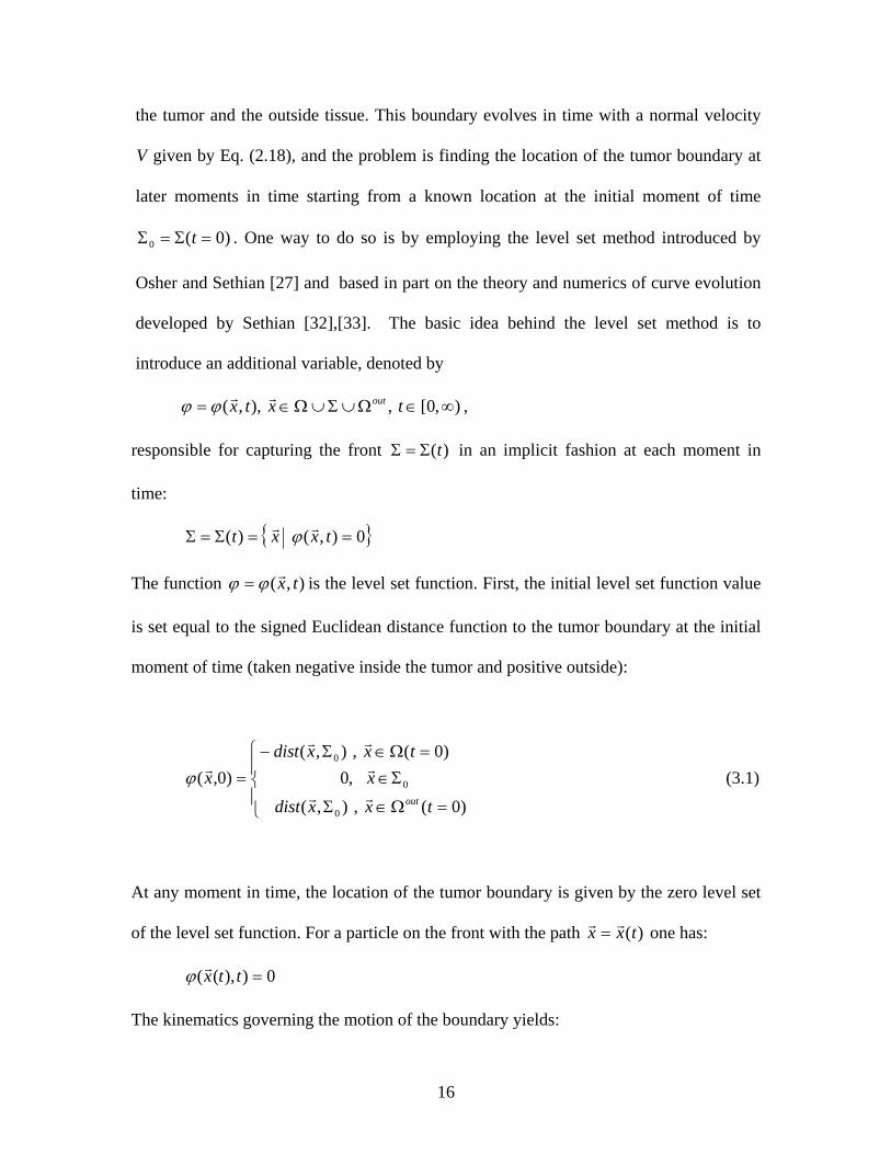
the tumor and the outside tissue. This boundary evolves in time with a normal velocity

given by Eq. (2.18), and the problem is finding the location of the tumor boundary at

later moments in time starting from a known location at the initial moment of time

. One way to do so is by employing the level set method introduced by

Osher and Sethian [27] and based in part on the theory and numerics of curve evolution

developed by Sethian [32],[33]. The basic idea behind the level set method is to

introduce an additional variable, denoted by

V

)0(0 =Σ=Σ t

),0[,),,( ∞∈Ω∪Σ∪Ω∈= txtx outrrϕϕ ,

responsible for capturing the front )(tΣ=Σ in an implicit fashion at each moment in

time:

0),()( ==Σ=Σ txxt rr ϕ

The function ),( txrϕϕ = is the level set function. First, the initial level set function value

is set equal to the signed Euclidean distance function to the tumor boundary at the initial

moment of time (taken negative inside the tumor and positive outside):

⎪⎩

⎪⎨

⎧

=Ω∈Σ

Σ∈=Ω∈Σ−

=

)0(,),(

,0)0(,),(

)0,(

0

0

0

txxdist

xtxxdist

xoutrr

r

rr

rϕ (3.1)

At any moment in time, the location of the tumor boundary is given by the zero level set

of the level set function. For a particle on the front with the path )(txx rr= one has:

0)),(( =ttxrϕ

The kinematics governing the motion of the boundary yields:

16

0,0)()),(( >∀=•∇+∂∂

= ttdtxdttx

tdtd r

rϕϕϕ

The outward unit normal on the boundary is given in terms of the level set function by:

ϕϕ

∇∇

=nr (3.2)

Substituting (3.2) in the above equation leads to the evolution equation for the level set

function (initial value formulation):

0=∇+∂∂ ϕϕ F

t (3.3)

where 0,),,( >Ω∪Σ∪Ω∈= txtxFF outrr represents what is typically called an

“extension velocity” field (i.e., defined everywhere, such that it always matches the

given expression of the normal velocity V on the tumor boundary Σ ):

)()( ),(),( txtx txVtxF Σ∈Σ∈ = rrrr (3.4)

Eq. (3.3) correctly moves the boundary with the prescribed normal velocity given by

(2.18).

As compared to an explicit front-tracking formulation, there are considerable advantages

of the level set formulation for this problem:

• the domain occupied by the tumor at each moment of time and the corresponding

outer environment are apparent from the sign of the level set function (here taken

negative the tumor region and positive outside);

• the local geometric properties of the tumor boundary (e.g. the normal) are readily

available;

• the same formulation holds regardless of the number of spatial dimensions (1,2 or

3);

17

• enhanced implementations such as “the narrow band method” introduced by

Adalsteinsson and Sethian [1] or “the fast marching method” [2],[34] are available

that make the boundary capturing more computationally efficient.

On the other hand, some challenges arise when implementing the level set method:

• construction of the “extension velocity” field in the level set equation (3.3)

(generally, there is no natural choice for this field which is only defined on the

interface itself);

F

• re-initialization of the level set function ϕ as a signed distance to the interface.

4. The spherically symmetric case

Solution procedures to the model equations (2.12) and (2.15) with the corresponding

initial and boundary conditions are developed in this section under the assumption of

spherical symmetry; both for computational purposes – to test the applicability of a level

set approach – and for biological ones – to check the model behavior. The tumor is

regarded as a growing sphere, of radius , with a given initial radius . The model

dependent variables ,

)(tR 0R

),( trUU AA = ),( trUU CC = ,U ),( trUTT = , and

, where

),( trUU DD =

),( trUU NN = r denotes the radial coordinate. The domain occupied by the tumor

is then )(0)( tRrrt ≤≤=Ω=Ω , embedded into a larger fixed sphere of given radius

: DR DRrrD ≤≤= 0 .

18

Each of the governing equations (2.12) and (2.15) can be cast in the general compact

form:

)()()()( µµνµµµ LWQt

−Γ+∇•∇−∇•∇=∂∂ (4.1)

where is constant and positive in Eqns. (2.12), zero in the first two Eqns. (2.15)

variable in the last equation (2.15); W is constant and positive in the second equation

(2.12), constant and negative in the first equation (2.15) and zero in all the remaining

equations;

Q

ν depends explicitly on µ only in the first equation (2.15). In (4.1), µ and ν

represent the various model dependent variables to be determined numerically. Rewriting

(4.1) in spherical coordinates under the assumption of spherical symmetry

( ),( trµµ = , ),( trνν = ,( trQ=,Q ) yields: )

)()()(1)(1 22

22 µµνµµµ L

rr

rrW

rQr

rrt−Γ+

∂∂

∂∂

−∂∂

∂∂

=∂∂ (4.2)

For discretization purposes, it is convenient to rewrite (4.2) in non-conservative form:

)()()2(22

2

2

2

µµνµνµνµµµµµ Lrrrrr

Wr

Qrrr

Qr

Qt

−Γ+∂∂

+∂∂

∂∂

+∂∂

−∂∂

+∂∂

∂∂

+∂∂

=∂∂ (4.3)

The form (4.3) is preferred here mainly for two reasons: the contribution of lower order

terms is individually highlighted for each of the model dependent variables – which

makes a heuristic stability assessment [30] easy to conduct when a fully-explicit finite

difference scheme is employed to solve numerically the nonlinear equations (4.3); then,

in an Eulerian formulation, with a fixed grid and a moving boundary captured implicitly

via a level set method, the spatial finite difference scheme at grid points adjacent to the

boundary must be modified to take into account the prescribed boundary conditions. The

latter is accomplished here by separately constructing second order interpolating

19

polynomials for each of the model dependent variables – or, in the framework of Eq.

(4.1), for each of the unknowns µ and ν . It is clearly then why a non-conservative

version of (4.1), that will highlight the first order derivatives of µ and ν separately, is

employed. However, an alternate ghost fluid method (GFM) formulation [26] allows for a

conservative form.

Another aspect of primary importance when proceeding to the spatial discretization of the

model Eqns. (2.12) – that are valid in the entire fixed computational domain - is

deciding whether to discretize them separately inside the region occupied by the tumor

and outside respectively. This is the approach employed here, for the following reasons:

in more general cases, the diffusion coefficients of TAF and of the new capillaries might

be different inside the tumor and in the outer environment respectively; then, the

production (source) term in the TAF equation is discontinuous across the tumor

boundary; and finally, splitting the larger problem into two smaller ones – a domain-

decomposition approach – is certainly very valuable in the perspective of a semi-

implicit/implicit time discretization.

D

All the numerical results presented in this paper are obtained by employing a fully

explicit (forward Euler) time discretization; alternate time-splitting/linearization schemes

are currently under investigation by the authors – but the nonlinear diffusion type term

in the equation for the living tumor cells (the first

equation (2.15)) coupled with the need to modify the spatial stencil at fixed grid points

adjacent to a moving boundary make the problem challenging and computationally

intensive; moreover, assessing the overall correctness and consistency [30],[38] of such

schemes is a delicate aspect, particularly when no other results exist for comparison.

))ˆ(( CCDTT UUUUU +++∇•∇

20

While the fully explicit method in an Eulerian framework with a moving boundary

certainly leads to severe constraints on the time step, it naturally handles the fully

nonlinear problem and the overall computational efficiency might prove equivalent to

that involved in a less constrictive time-splitting method; the numerical results presented

here shall show that a fully explicit method can be used as a basic computational tool to

investigate the model behavior for model parameters in a certain range, particularly when

no previous simulations have been performed and at least a preliminary assessment of the

model from a biological point of view is desired.

4.1 A pseudo-Lagrangian solution method

For the spherically symmetric case it is possible to employ a coordinate transform

and fix the location of the tumor boundary in the transformed domain (Landau

transformation). A solution procedure using this method was developed for comparison

purposes with the level set approach. For the tumor boundary location defined by R(t),

the following transformed coordinates are defined:

21,

)()(1

10,)(

≤≤−

−+=

≤≤=

ηη

ξξ

tRRtRr

tRr

D

(4.4)

21

At each moment of time , the inside of the tumor is being mapped onto the interval

the outside of the tumor is being mapped onto the interval and the tumor boundary

is located at

t ]1,0[ ,

]2,1[

1== ηξ . Employing the chain rule in (4.3) yields:

10,)()(

)]2(2[)(

1)()(

2

2

2

2

2

<<−Γ+∂∂

+∂∂

∂∂

+∂∂

−∂∂

+∂∂

∂∂

+∂∂

+∂∂

=∂∂

ξµµξνµ

ξξν

ξµ

ξνµ

ξµ

ξξµ

ξξµ

ξµξµ

L

WQQQtRtR

tRt

&

(4.5)

and

21,)()()()(

1))()(1()(

2

)]([))((

1)(

)()2( 2

2

2

2

2

<<−Γ+∂∂

−∂∂

−−−++

∂∂

∂∂

+∂∂

−∂∂

∂∂

+∂∂

−+

∂∂

−−−=

∂∂

ηµµηνµ

ηµ

η

ην

ηµ

µνµ

µµ

ηηµ

ηµηµ

LWQtRRtRRtR

WQQtRRtRR

tRt

DD

DD

&

(4.6)

where )()( tdtdRtR =& .

Clearly, the model governing equations (2.15) satisfied inside the domain occupied by the

tumor only are of the form (4.5), while the model equations (2.12) – valid in the entire

computational domain – are split into two: inside the domain occupied by the tumor and

outside respectively, thus they are of the form (4.5) - inside and (4.6) – outside. In this

case, additional matching conditions at the tumor boundary are needed for the

corresponding model dependent variables and respectively; these will be

obtained by naturally assuming continuity of and and of the related fluxes

AU CU

Au Cu

22

nuk AAr

•∇ )( and nuuwuk ACCCCr

•∇−∇ )( across the tumor boundary, which here leads

to:

⎪⎪⎪

⎩

⎪⎪⎪

⎨

⎧

∂∂

−=

∂∂

∂∂

−=

∂∂

==

==

==

====

11

11

1111

)(1

)(1

)(1

)(1

,

ηξ

ηξ

ηξηξ

ηξ

ηξ

C

D

C

A

D

A

CCAA

UtRR

UtR

UtRR

UtR

UUUU

(4.7)

Symmetry boundary conditions are employed at the tumor center 0=r :

000000 =∂

∂=

∂∂

=∂

∂=

∂∂

=∂

∂===== ξξξξξ ξξξξξ

NDTCA UUUUU (4.8)

According to Eq. (2.18), the tumor radius evolution in time is given by: )(tR

⎪⎩

⎪⎨

⎧

=

+++∂∂

−=∂∂

−==

=

==

00

),1(),1( )ˆ()(

1)(

1)()(

RR

UUUUtR

WUtR

WtdtdRtR

t

tCCDTTtT ξξ ξξ&

(4.9)

Description of the numerical algorithm:

• The “inner” domain 10 ≤≤ ξ and the “outer” domain 21 ≤≤ η are each

discretized using equally spaced meshes; the interface is a mesh point,

corresponding both to 1=ξ and 1=η .

23

• The interface motion equation (4.9) is discretized using forward differencing in

time and second order backward differencing in space (since the global cell

density is discontinuous across the interface); therefore,

the new location of the interface at the current time step is obtained by using the

location of the interface at the previous time step and the global cell density at the

previous time step.

CCDT UUUUU ˆ+++=

• The “inner” set of model governing equations (4.5) is discretized at all the internal

mesh points using forward differencing in time and regular second order centered

differences in space both for the second order and for the first order derivatives;

similarly for the “outer” set (4.6); thus, the new values of the model state

variables at the current time step are determined at all internal mesh points – both

inner and outer. To update the current values of the state variables at the interface

– which is both an “inner” mesh point and an “outer” mesh point, the matching

conditions (4.7) are first used to determine the current values of and

respectively at the interface; once the value for is known at the current time

step, then the model boundary conditions (2.16) are used to update the values of

and at the interface at the current time step.

AU CU

CU

TU NU

The implementation of the above algorithm is straightforward; the numerical stability and

ultimately the convergence of the explicit method depends on the choice of the model

parameters. More comments follow in the results section 4.3.

4.2 A level set (Eulerian) solution approach

24

The detailed description of the numerical algorithm for the fixed Cartesian

mesh/level set approach in two dimensions and arbitrary geometries is addressed in

Section 5 and Appendix A. The same general formulation holds regardless of the number

of spatial dimensions (1,2 or 3). Below the formulation is outlined for the spherically

symmetric case; this is done from a computational perspective for comparison purposes

and to assess the applicability of the proposed computational methodology for the current

complex tumor growth model.

As in section 4.1 above, symmetry conditions are employed at the tumor center . 0=r

As previously, continuity of and and of the related fluxes across the tumor

boundary , which here translates into the continuity of , ,

Au Cu

)(tRr = AU CUr

U A

∂∂ and

rUC

∂∂ at , shall also be employed. )(tRr =

Description of the numerical algorithm:

• The entire fixed computational domain DRr ≤≤0 is discretized using equally

spaced meshing; the interface )(tRr = in this case is generally not a mesh point.

• The new location of the interface at the current time step is given by the zero level

set function at the current time step; the level set equation (3.3) in this case reads:

0=∂∂

+∂∂

rF

tϕϕ (4.10)

where F is the extended velocity field, here extended off the tumor boundary such

that it is constant on normal rays to the tumor boundary; as a consequence of the

25

spherical symmetry, the extended velocity everywhere is then taken equal to the

normal velocity of the tumor boundary:

)(TrrT rUWF =∂

∂−= (4.11)

The initial level set function is given by 0)0,( Rrtr −==ϕ . To update the time-

dependent level set function ϕ , a simple explicit first order scheme in time

(forward Euler) and space is used to discretize the level set equation (4.10) (refer

to Section 5 for more information). The spatial derivative in (4.11) is

approximated using second order backward differencing

( is discontinuous across the interface). With the level set

function updated, the new location of the interface is estimated as the zero level

set by linear interpolation of the new level set function.

CCDT UUUUU ˆ+++=

• The set of model governing equations (4.3) is discretized using forward

differencing in time and regular second order centered differences in space both

for the second and for the first order derivatives at all the internal mesh except the

ones adjacent to the boundary. At points adjacent to the boundary, the spatial

discretization must be modified to take into account the location of the boundary

and the model prescribed boundary conditions. As already mentioned, this is

accomplished by constructing local second order interpolating polynomials for

each of the model dependent variables , , , and respectively;

then their second order derivative at a point adjacent to the boundary is

approximated as the second order derivative of the corresponding polynomial;

similarly for the first order derivatives.

AU CU TU DU NU

26

To update the current values of the state variables at the interface – which are to

be used at the next time step in constructing the local second order interpolating

polynomials at points adjacent to the boundary - the continuity of , , AU CU

rU A

∂∂ and

rUC

∂∂ at the tumor boundary is first used to determine the current values

of and respectively at the interface; once the value for is known at the

current time step, then the model boundary conditions (2.16) are used to update

the values of and at the interface at the current time step.

AU CU CU

TU NU

Details can be found in Appendix A.

4.3 Numerical results

4.3.1 Numerical results from a computational point of view

The first aspect to be addressed is the usage of centered finite differences to

approximate the first order derivatives in equation (4.3). If an heuristic stability

assessment is conducted for each of the model equations (2.12) and (2.15) considered

separately [30], then potential stability problems may arise if the advection terms

dominate diffusion terms. An estimate for the magnitude of the relevant model

parameters is necessary to fully access the stability. For the parameters considered here,

the diffusion type constraint on the time-step imposed by the first equation in (2.12) will

generally dominate the advection-diffusion type constraint for the second equation in

(2.12). Under these conditions, the use of centered finite differences in approximating the

27

first order derivatives is relatively safe. Numerical experiments support this conclusion.

However, to investigate model behavior in regimes characterized by drift coefficients

(e.g., ) substantially larger than the model diffusion coefficients, then upwind schemes

must be used to discretize the first order spatial derivatives in the second equation (2.12).

CW

A second aspect of computational concern is the treatment of the terms involving the

Heaviside function in the first and second equation (2.15). It is common to smear out the

Heaviside function for computational implementation purposes by defining:

))arctan(21(21)(

επuuH +≈ (4.15)

with ε a small value (typically, )(hO=ε , where represents the spatial mesh size). h

However, in our numerical experiments performed so far, by comparing the results

obtained using the actual Heaviside function and the smeared out version given by (4.15),

no significant differences were detected.

Another important aspect is the choice of the larger fixed computational domain –

because of the boundary conditions (2.13). In the spherically symmetric case (i.e., 1D), it

is easy to employ a radius for the fixed outer domain considerably larger than the initial

radius of the tumor – such that both the density of TAF and the density of the new

capillaries naturally decay to zero towards the outer domain boundary. In higher

dimensions, the choice of the domain size for the outer environment is more restricted.

Numerical tests performed in the spherically symmetric case (and in 2D) have

demonstrated the requirements on the choice of the outer boundary location.

AU

CU

Fig.1 shows a comparison between the tumor radius in time obtained via the pseudo-

Lagrangian method described in section 4.1 and the tumor radius in time obtained via the

28

Eulerian/level set method described in section 4.2 for the following choice of the model

parameters (2.19):

2.0,1,10 === NCA KKK

10,5 == TC WW

100=ΓC

001.0,10,5,01.0,01.0 =∆=∆=∆=∆=∆ DNTCA (4.16)

⎩⎨⎧ <<

==otherwise

RrRifrUU CC 0

45.3,1.0)(ˆ,1 00

1,9.0~,8.0 === BUU NN

10,20 == DRR

The spatial mesh size in the pseudo-Lagrangian method is 02.0=∆=∆ ηξ with a fix

time-step , while in the Eulerian/level set method 51066.2 −×=∆t 05.0=∆r with the

time-step chosen adaptively (obeying stability restrictions). These choices for the mesh

sizes, initially balances the number of mesh points inside the physical domain occupied

by the tumor for the two methods (the resolution remains balanced during a reasonable

portion of the tumor evolution). The results show very good agreement between the two

different solution methods.

4.3.2 Numerical results from a biological viewpoint

29

All the results discussed in this section are obtained using the above set (4.16) of model

parameters as base values. Any parameter variation is explicitly defined when presenting

the results.

i. Evolution of the tumor radius in time

In Fig.1 two different stages of tumor growth can be clearly distinguished: up to time

, the growth is linear, at a relatively low rate – corresponding to the avascular

stage; at later times, the growth is accelerated, exhibiting exponential trends –

corresponding to the vascular stage. Fig. 2 shows the behavior of the tumor radius in time

in the absence of tumor-induced angiogenesis, for two different values of : the solid

line corresponds to a value of

84.1≈t

D∆

001.0=∆ D and the dashed line to 1=∆D ; the rest of the

model parameters are as in (4.16) above. In the case of the large disintegration rate

for the tumor dead cells, the tumor radius shows stabilization to a limiting value

of around time , while in the case of the small disintegration rate

approach to a stabilized state is not yet apparent up to time

1=∆D

3≈R 10=t 001.0=∆ D

20=t . This is in good

agreement with the argument made in [11], that ultimately a balance between the living

tumor cells and the dead tumor cells – reached when the proliferation of cells near the

tumor surface balances the disintegration of dead cells in the necrotic region – determines

a stationary radius of the avascular tumor. For the same value of the drift coefficient

, smaller values of lead to a larger stationary radius of the tumor and a larger

necrotic core with respect to the proliferation rim.

TW D∆

ii. Tumor living and dead cell density evolution

30

Fig. 3 plots the tumor living cell density versus the radial coordinate TU r at various

moments in time. The avascular and the vascular stages of growth are clearly

differentiated here as well; in the avascular phase, decreases towards the center of the

tumor because the living tumor cells start to gradually die when they lack nutrients – this

is confirmed by the corresponding evolution of the dead tumor cell density shown in Fig.

4; further, in the vascular phase, it is observed that the living tumor cell density continues

to rapidly drop towards the center – while the dead cell density, , there remains

stationary (note that the model assumes dead tumor cells do not move). In the model,

living tumor cells towards the center stop dying, and migrate towards less populated areas

where they have a higher probability to survive and eventually continue the mitosis

process if the levels of nutrients are high enough. In Fig. 6, the overall cell density,

, is plotted at specific times; the curves show that once the new

capillaries penetrate the tumor and begin to influence its center there will be a rapid

increase of the overall cell density. Since the tumor size is relatively small here and the

upper threshold for the new capillaries is high, while their death coefficient is much

smaller than the growth coefficient, this happens relatively fast. The rapid increase in

overall cell density leads to sharper local gradients, that in turn lead to fast movements of

the living tumor cells towards the outer tumor region; in particular, there is a significant

increase in the slope of the overall tumor cell density at the boundary of the tumor. Recall

from Eqn (2.18) that the velocity of the tumor boundary is directly proportional to the

gradient of the overall cell density.

TU

DU

CCDT UUUUU ˆ+++=

iii. New capillary cell evolution

31

The evolution of the new capillaries is depicted in Fig.5. To facilitate the simulation, a

large value for the growth coefficient CΓ was chosen while the death coefficient C∆ is

small. In addition, the drift coefficient, , is five times larger than the diffusion

coefficient, . These parameters yield significant movement of the new capillaries

towards the source of angiogenic stimulus (TAF), which is maximum inside the domain

occupied by the tumor. In the model, the density of new capillaries is allowed to reach an

upper threshold

CW

CK

1=CU , which is the close packing density for the overall cell density, so

the resulting scenario is not totally realistic. However, the choice of parameters related to

the growth of new capillaries (which is, in fact, the core of the tumor vascularization

problem) allows for the overall development of visible and meaningful changes over a

relatively short period of time.

iv. The TAF and nutrient concentration evolution

The TAF distribution along the radial coordinate at various times is shown in Fig. 7. In

the present version of the model, it is assumed that the living tumor cells constantly

produce and release TAF, which diffuses at the same constant rate both inside the tumor

and in the surrounding outer environment. Because of this assumption and the fact that

the TAF decay parameter is chosen small ( 01.0=∆ A ) for the case considered, the

evolution equation for TAF (the first equation (2.12)) is a linear diffusion equation with a

source term with vanishing boundary conditions. As a result, the TAF concentration

maintains a maximum at the tumor center.

The nutrient evolution is presented in Fig.8. Fig.8(a) shows the radial distribution of

the nutrient at various times during the avascular phase. The nutrient reaching the tumor

32

surface diffuses inside the tumor;. Since the evolution equation for the nutrient inside the

tumor (the last equation (2.15)) is a diffusion equation with a sink term, the levels of

nutrient maintain a maximum at the tumor boundary and gradually decrease towards the

tumor center. As a consequence, living tumor cells first start dying at the center, while a

layer of cells adjacent to the boundary are able to proliferate. Fig.8(b) shows the nutrient

evolution at later times, in the vascular phase; with the accelerated development of new

capillaries, increased amounts of nutrients reach the tumor surface and diffuse inside the

tumor at a rate increasing proportionally to the new capillary density. This explains why

the tumor dead cell density remains almost stationary from a point on (the level of

nutrient becomes sufficient for the remaining living cells).

5. Description of the general numerical algorithm and discretization procedures

5.1 Construction of the “extension velocity” field off the interface

One way of extending the normal velocity off the interface in the level set

equation (3.3) is extrapolation in the normal direction, following characteristics that flow

outward from the interface, such that the velocity is constant on rays normal to the

interface. This method, introduced by Malladi, et al. [23] works particularly well when no

other information is available except for what is known on the interface–as is the case

here. At points adjacent to the interface, on each side, the “extension velocity” field is

first constructed as follows: standing at a grid point adjacent to the interface, either inside

F

33

the domain occupied by the tumor or outside, locate the closest point on the interface

whose velocity is given by Eq. (2.18) – with second order backward differencing in the

normal direction used to numerically approximate the normal derivatives – and copy its

velocity. Construction of the extension velocity field in this manner has the advantage

that it tends to preserve the signed distance function during the interface evolution in

time. A fast way of building these extension velocities in the context of Dijkstra's-like

algorithms was provided by Adalsteinsson and Sethian in [2]. An alternate way to

formulate this construction is by employing a pair of linear Hamilton-Jacobi equations

[26], in which the velocity values at the adjacent points are subsequently kept fixed and

framed as boundary conditions for the following:

)(0 tinFnF outΩ=∇•+∂∂ r

τ (5.1)

)(0 tinFnFΩ=∇•−

∂∂ r

τ (5.2)

where the local unit outward normal in the level set methodology is defined everywhere

as:

),(),(),(

txtxtxnn r

rrrr

ϕϕ

∇∇

== (5.3)

Here τ designates a pseudo-time for the relaxation of the equations to steady-state at each

moment of time t . Equations (5.1) and (5.2) are numerically discretized using a regular

first order upwind scheme [22],[26] and iterated to steady-state, where the corresponding

solution ), tx(FF r= will be constant on rays normal to the interface.

The normal ),( txnn rrr= in (5.3) is approximated using the construction described in

[31]; the local unit outward normal at a point on the interface - which generally is not a

34

grid point - is obtained by bilinear interpolation from the values of the local unit outward

normal computed at the four neighboring nodes on the fixed Cartesian grid.

5.2 Re-initialization of the level set function ϕ

As discussed by Chopp [13], in general, a procedure is needed to reset the level

set function ϕ as a signed distance function to the interface (in this case, the tumor

boundary) from time to time. Re-initialization at some moment of time can be regarded

as the process of replacing the current level set function

t

),( txrϕ by another function

),( txreinit rϕ that has the same zero contour but is better behaved; ),( txreinit rϕ becomes the

new level set function to be used as initial data until the next re-initialization.

Reinitialization and its role in Narrow Band Methods was first analyzed in depth by

Adalsteinsson and Sethian in [2], and a very fast Dijkstra-like method to perform this

reinitialization was given by Sethian in [34].

Another way of re-initializing the level set function ϕ to a signed distance function to the

interface employs the following “re-initialization equations” [26]:

)(0)1( tin outreinitreinit

Ω=−∇+∂

∂ ϕτ

ϕ (5.4)

)(0)1( tinreinitreinit

Ω=−∇−∂

∂ ϕτ

ϕ (5.5)

with

),()0,(0 txxreinitreinit rr ϕτϕϕ === (5.6)

35

Here again, τ designates a pseudo-time for relaxing the equation to steady-state at a fixed

real time . As before in the case of the extension velocity, first at grid points adjacent to

the boundary, on each side, is reset close to a signed distance function by hand (a

very efficient way is the initialization stage of the fast marching method in [31]). These

values are subsequently kept fixed and framed as boundary conditions for the equations

(5.4) and (5.5) respectively, that are individually solved to steady-state. The resulting

solution

t

reinitϕ

),( txreinit rϕ will be a signed distance function to the interface at the

particular time t in the model evolution.

)(tΣ=Σ

The implementation of the level set methodology is presented here for the two-

dimensional case, but the extension to three dimensions is straightforward. The domain

occupied by the tumor Ω is embedded into a larger fixed, time-independent,

computational domain D, that is discretized using a uniform Cartesian mesh with

The region outside of the tumor is denoted by .hyx =∆=∆ =Ωout D . The tumor

boundary will also be referred to as the “interface” – separating the domain occupied by

the tumor from the outside tissue. A “regular” grid point (either inside the domain

occupied by the tumor or outside) shall denote a point on the fixed Cartesian grid that has

no neighbors on the tumor boundary, in either the horizontal (

Ω\

x ) direction or the vertical

( ) direction, while an “irregular” grid point (on each side of the tumor boundary)

corresponds to a point on the fixed Cartesian grid that is adjacent to the boundary, either

horizontally or vertically.

y

5.3 Discretization of the level set equation and the re-initialization equation

36

The level set equation (3.3) is discretized using a conservative scheme for

nonlinear Hamilton-Jacobi equations with convex Hamiltonian [31]:

(5.7) ])0,min()0,[max( ,,,1

,−++ ∇+∇∆−= n

jinji

nji

nji FFtϕϕ

where:

)9.5(])0,min()0,max()0,min()0,[max(

)8.5(])0,min()0,max()0,min()0,[max(

)),(),((

)),(),((

21

2,

2,

2,

2,

21

2,

2,

2,

2,

,

,

nji

ynji

ynji

xnji

x

nji

ynji

ynji

xnji

x

nji

nji

DDDD

DDDD

tnjyixFF

tnjyix

ϕϕϕϕ

ϕϕϕϕ

ϕϕ

−+−+−

+−+−+

+++=∇

+++=∇

∆=

∆=

and ( ) stands for the backward differencing approximation of the first-order

partial derivative in the x (y)–direction, while ( ) stands for the forward

differencing approximation. The above scheme is a first order (forward Euler) in time;

higher order schemes such as HJ ENO or WENO can be employed [26]. The time step in

(5.7) must obey the CFL condition for stability:

xD− yD−

xD+ yD+

2

max ,,

hFt njiji

≤∆ (5.10)

A similar scheme is used to discretize the re-initialization equations (5.4) and (5.5).

5.4 Overall numerical solution procedure

The governing model equations are discretized using explicit finite difference

schemes, which enables straightforward implementation. Details of the numerical

37

solution procedure for the model dependent variables are given in Appendix A. A

comparison of spatial discretization schemes for the level set equation and a discussion of

the approximation error is given in [17]. Here, the global solution algorithm is outlined

briefly in terms of the following steps:

1) It is assumed that all the model dependent variables: ),( txU Ar , ),( txUC

r , ),( txUTr ,

, ),( txUDr ),( txU N

r (all initially given by the model initial conditions (2.14) and (2.17))

along with the level set function ),( txrϕ are known at time t , with the level set function

equal to the signed distance function (prescribed initially, or as a result of re-initialization

at later times). As a result, the current location of the interface is implicitly known.

Following [1], a “narrow band” (tube) is built around the interface, with a user-prescribed

width. Since ),( txrϕ is assumed close to a signed distance function, the narrow band is

defined by locating the points using the following criterion:

Twidthtxxnot.

),( =<rr ϕ .

The grid points inside the tube and the grid points near the tube edge are marked

distinctly.

2) With the value of )(ˆ),(),(),(),( xUtxUtxUtxUtxU CCDTrrrrr

+++= known at the time

step , the “extension velocity” field t ),( txFF r= is constructed as described in Section

5.1, at points inside the narrow band tube xr T .

38

3) With the extension velocity field computed at points inside the tube T , the level set

equation (5.7) is solved inside the tube to update the level set function at the next time

step. The values of the level set function at grid points distinctly marked near the tube

edge in Step 1 are frozen, as well as the values of the level set function outside the tube

T . The following conditions are monitored:

a) whether the newly updated tumor boundary (interface) approaches the tube edge

to within a specified tolerance (if so, then the values kept frozen in Step 4, which

serve as artificial numerical boundary conditions, will severely affect the actual

location of the interface);

b) whether steep or flat gradients are developing in the newly updated level set

function, particularly at points neighboring the interface.

4) With the new location of the boundary implicitly captured by the updated level set

function ),( ttx ∆+rϕ , the model governing Eqs. (2.12) and (2.15) along with the

corresponding prescribed boundary conditions (2.13) and (2.16) are employed to compute

the new values of the model dependent variables: ),( ttxU A ∆+r , ),( ttxUC ∆+

r ,

, ),( ttxUT ∆+r ),( ttxU D ∆+

r , ),( ttxU N ∆+r as described in Section 5.4 .

Steps 2-4 are repeated until either situation a) or b) occurs; when this happens, the narrow

band (tube) T must be rebuilt and the procedure begins with Step 1 again. Employing this

narrow band level set method is computationally very efficient (especially in constructing

39

the extension velocity field); this approach is ideal when only the evolution of the

interface itself is of interest (i.e., the zero level set), as is the case here.

6. Numerical results in two dimensions – arbitrary geometry

6.1 Computational Details

The numerical simulations presented here were obtained by employing

straightforward finite-difference schemes. The motivation was to create a framework that

could be easily implemented to study a variety of tumor growth models. For the present

model, since no curvature effects at the tumor boundary are incorporated, we find that a

first-order spatial scheme in the level set equation (5.7), as well as in the re-initialization

equations (5.4), (5.5) can be safely used. For the same reason, the size of the narrow band

(tube) T can be relatively modest – here a width of on each side of the interface is

chosen and the interface is only allowed within at most 2 grid cells from the tube

boundary (i.e., it is allowed to move at most 4 grid cells within the tube) before the tube

is rebuilt. As in [17], re-initialization is typically used jointly with re-building the narrow

band. They also determined that the forward Euler time integration scheme for the level

set equation (5.7) was sufficient; particularly since the time step is small due to the

overall fully explicit nature of the solution procedure.

h6

Regarding the choice of the “small” value ε in the ε -test (see Eq. (A.5) in Appendix

A), since the actual location of a boundary point is found by linear interpolation of the

level set function at the neighboring grid points, one natural consistent choice for ε is

40

)(~ 2hOε ; the results in the spherically symmetric case via the Eulerian/level set

approach in Section 4 are obtained by using . However, this choice is related

strictly to the spatial accuracy of the numerical approximation, and has no apparent

geometrical interpretation; in the context of Eq. (A.5), the geometrical location of a

boundary point (either in the horizontal or in the vertical direction) is in-between two

Cartesian grid points, and the actual measure of how close one of the two grid points is to

the boundary point is given by a fraction of the grid size . In our numerical experiments

we found that a good choice for

2h=ε

h

ε is Nh /=ε , with N an integer that depends on the

geometrical properties of the front involved. If no curvature effects are present – as in the

current model – then 5/h=ε was found to work well. This is demonstrated by the

results shown in Fig. 9, where the initial tumor boundary is taken to be a circle centered

at the origin with radius 1, and the support of pre-existing capillaries is a circular area

surrounding the initial tumor: 3.22),( 22 <+<= yxyxS . The set of model

parameters (4.16) is used, but with the pre-existing capillary density taken five times

larger, to speed up the calculations ( inside S ). A comparison is performed

between the tumor radius evolution obtained by three different sets of calculations: the

two-dimensional Cartesian level set approach described in Section 5, the one-dimensional

Eulerian/level set approach described in Section 4.2 (under the assumption of polar

symmetry) and the one-dimensional pseudo-Lagrangian method described in Section 4.1

under the assumption of polar symmetry as well. For the 2D method, the fixed Cartesian

mesh size is , the computational domain (outer environment) is

5.0ˆ =CU

05.0=h ]4,4[]4,4[ −×−

and the time step is adaptive; in the 1D Eulerian/level set method, the mesh size is

41

05.0=∆r , the radius of the outer environment is 4=DR and the time step is adaptive; in

the 1D pseudo-Lagrangian method, the mesh size is 04.0=∆=∆ ηξ and the time step is

. The results demonstrate that the two-dimensional problem formulated in

Cartesian coordinates in this case exhibits genuine polar symmetry while in the avascular

phase of the tumor growth (see model equations (2.15) – (2.17)), but it gradually starts to

depart from it with the increased development of new capillaries in the subsequent

vascular phase. This is due to the geometric computational configuration of the outer

environment in Cartesian coordinates, which is a fixed square box, and not a circle (how

long the assumption of full polar symmetry can be employed depends on the size of the

fixed Cartesian computational box relative to the tumor radius). There is very good

agreement for the growth rate between the three sets of results up to time (which

corresponds to the avascular phase of growth); the agreement continues to be good

(within the overall accuracy of the methods) up to time

5104.6 −×=∆t

5.0≈t

9.0≈t . Eventually, the two-

dimensional Cartesian result no longer compares to the one-dimensional results obtained

under the assumption of full polar symmetry.

Similarly with the argument made in [17], when computing the normal velocity of the

tumor interface via Eq. (2.18), a second-order accurate backward difference

approximation in the normal direction is found optimal here as well. If the field variables

, and are numerically computed with second-order spatial accuracy, then the

numerical estimate of the normal velocity of the interface can only be at most first-order

accurate. Thus, it is to be expected that the location of the tumor boundary can be found

at most with first-order spatial accuracy.

TU DU CU

42

All the results that follow are obtained within the framework of the general Eulerian

level set/Cartesian grid methodology described in Section 5 above. In Fig. 10, the results

of a convergence study are shown. The tumor initial boundary is given by the 4-fold

symmetrically perturbed circle:

]2,0[)),sin(),))(cos(4

4sin(4.0)4

4cos(4.08.4())(),(( παααπαπααα ∈+−+−=yx (6.1)

The same model parameters as in Fig. 9 above are used. Outside the domain occupied

initially by the tumor there are four fixed circular seeds of pre-existing capillaries,

symmetrically positioned and relatively close to the boundary of the outer environment.

This initial configuration will be described in more detail below. The evolution of the

tumor boundary computed using three different mesh sizes: 4.0=h , and 2.0=h 1.0=h

is shown at three different moments of time and the qualitative convergence can be

observed. The mesh sizes were chosen to allow for two levels of refinement, starting with

a reasonable mesh spacing. Currently, the methodology developed here is designed for

implementation on moderately sized, standalone computing platforms. Moderate mesh

resolution, relative to the initial tumor size, was used to evaluate the solution behavior

and determine whether the results show the correct qualitative trends.. Through numerical

testing, it was found that the location of the tumor boundary was not very sensitive to the

spatial mesh size, when the value of the drift coefficient equal to 10 or smaller, since

there is no curvature effect at the boundary in the current model. In [17], where the tumor

boundary curvature was important, for drift coefficients of the same order of magnitude,

considerable sensitivity to the spatial resolution was found.

TW

The accuracy of the tumor boundary location in time can be quantitatively estimated

[17]. The level set method reconstructs the interface at every moment of time as a

43

piecewise linear manifold; suppose that the Cartesian mesh size is doubled twice and

denote by 1,1

1,,int Nk

nkerfacex

=

r , 2,1

2,,int Nk

nkerfacex

=

r and 4,1

4,,int Nk

nkerfacex

=

r the collection of

interface points

),( ,int,int,int kerfacekerfacen

kerface yxx =r at time ntt = corresponding to the coarsest mesh, the

intermediate mesh and the finest mesh, respectively. Thus, the interface is represented as

a polygonal line with , and line segments for the coarsest, intermediate and

finest representation, respectively. Each polygonal line can be re-divided into the same

given number

1N 2N 4N

N of equally spaced points (typically 4NN = ) and the newly determined

points on each polygonal line are correspondingly marked as Nkn

kerfaceX ,11,

,int =

r,

Nkn

kerfaceX ,12,

,int =

r and Nk

nkerfaceX ,1

4,,int

=

r, respectively.

Since no analytic solution is available, the errors are computed with respect to the

numerical solution corresponding to the finest mesh Nkn

kerfaceX ,14,

,int =

r; following [18], the

error at time is defined as the largest Euclidean distance of the corresponding

points of the two computed interfaces:

ntt =

4,,int

1,,int,11_4 max n

kerfacen

kerfaceNk

n XXerr

−==

(6.2)

4,,int

2,,int,12_4 max n

kerfacen

kerfaceNk

n XXerr

−==

(6.3)

44

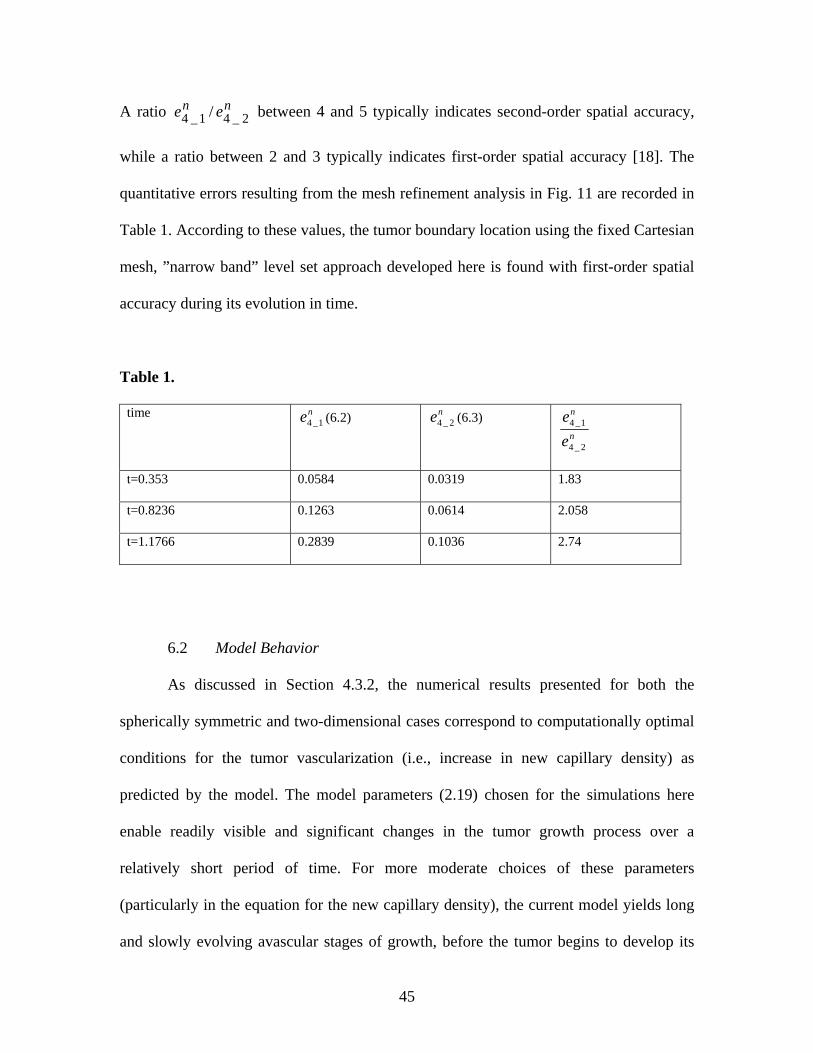
A ratio between 4 and 5 typically indicates second-order spatial accuracy,

while a ratio between 2 and 3 typically indicates first-order spatial accuracy [18]. The

quantitative errors resulting from the mesh refinement analysis in Fig. 11 are recorded in

Table 1. According to these values, the tumor boundary location using the fixed Cartesian

mesh, ”narrow band” level set approach developed here is found with first-order spatial

accuracy during its evolution in time.

nn ee 2_41_4 /

Table 1.

time ne 1_4 (6.2) ne 2_4 (6.3) n

n

ee

2_4

1_4

t=0.353 0.0584 0.0319 1.83

t=0.8236 0.1263 0.0614 2.058

t=1.1766 0.2839 0.1036 2.74

6.2 Model Behavior

As discussed in Section 4.3.2, the numerical results presented for both the

spherically symmetric and two-dimensional cases correspond to computationally optimal

conditions for the tumor vascularization (i.e., increase in new capillary density) as

predicted by the model. The model parameters (2.19) chosen for the simulations here

enable readily visible and significant changes in the tumor growth process over a

relatively short period of time. For more moderate choices of these parameters

(particularly in the equation for the new capillary density), the current model yields long

and slowly evolving avascular stages of growth, before the tumor begins to develop its

45

own capillary network. During the avascular stage the growth is stable, with a linear rate

of growth initially, that decreases asymptotically to zero. It is the vascularization of the

tumor via the tumor induced angiogenesis contained in the model that leads to more rapid

and unbounded growth. From a computational standpoint, the stability requirements due

to the fully explicit nature of the numerical scheme lead to certain practical bounds on the

choice of the model parameters used in the actual simulations.

For the 2-D simulation results presented in Figs.11 and 12, the same set of model

parameters used for the case shown in Fig. 9 was used. In Fig. 11(a), the evolution of the

tumor with the initial boundary given by Eq. (6.1) is shown in detail. Outside the domain

occupied initially by the tumor there are four circular seeds of pre-existing capillaries,

symmetrically positioned and relatively close to the boundary of the outer environment;

their location is marked by the small gray circles, of centers: (6,6), (-6,6), (-6,-6) and (6,-

6) respectively, and radius 1.2; the Cartesian mesh size 1.0=h , the computational

domain (outer environment) ]8,8[]8,8[ −×− and the time step is adaptive. The initial

tumor boundary is deliberately chosen as a circle symmetrically perturbed towards the

location of the pre-existing capillaries. Up to time 6.0≈t the tumor is in the avascular

phase−the growth is very slow, stable and self-similar. At time 9.0≈t , corresponding to

an intermediate to moderate degree of tumor vascularization, instability starts to become

evident as the initially perturbed tumor boundary grows more towards the location of the

pre-existing capillaries, exhibiting a tendency to elongate. However, at later times, in a

high vascularization phase, the elongation is less apparent and the tumor continues to

expand rapidly but in a relatively uniform manner. The explanation of the growth

behavior is found in the corresponding evolution of the new capillaries, depicted in Fig.

46

11(b), where both a contour map(11b-1) and a surface plot(11b-2) of the new capillary

density are included. It can be seen that the endothelial cells stimulated initially are the

ones belonging to the pre-existing capillaries. At early times, since the new capillaries

have not evolved sufficiently to reach the tumor, it remains in the avascular phase and the

slow stable growth occurs as described above. An intermediate stage of vascularization

follows when enough new capillaries have developed outside the tumor in the regions

neighboring the location of the pre-existing capillaries, such that they undergo a strongly

oriented movement towards the source of angiogenic stimulus – the tumor itself. It is in

this stage that the tumor exhibits the tendency to elongate towards the location of the pre-

existing capillaries. At later times, once the newly formed blood vessels (characterized by

the capillary density) have reached inside the tumor, they are in turn stimulated to

proliferate, and a faster tumor vascularization follows (due to the fact that the TAF values

are much higher inside the tumor than outside, coupled with the large value of the growth

coefficient, ). Eventually, the new capillary distribution tends to level-off

spatially leading to subsequent quasi-uniform growth of the tumor.

100=ΓC

Contour maps of the tumor living cell density are shown in Fig. 11(c). In the avascular

phase of the tumor growth, a rim structure develops as described in [11]. The results

show a very thin outer rim of proliferative cells, followed by a slightly thicker adjacent

rim of quiescent cells–cells that live but do not proliferate. The inner tumor region shows

a smooth transition towards a large necrotic core. The choice of the nutrient threshold

values 9.0~8.0 =<= NN UU in (4.16) allows for the existence of a quiescent rim of

living tumor cells (a tumor region where the nutrient levels reaching the existent living

47

cells are such that NUTUNUNU ~/ << ). The smooth transition towards a large necrotic

core is confirmed by the evolution of the tumor dead cells shown in Fig. 11(d).

The distinct patterning in the living and dead cell densities at later times results from

the development and the subsequent spatial distribution of the new capillaries. A local

increase of the new capillary density affects the value of the living cell density on the

tumor boundary due to the given boundary conditions. Inside the tumor, local gradients

of the overall cell density U develop and the living tumor cells are redistributed

accordingly. The pattern of the living tumor cells in turn impacts the pattern of the dead

cells; moreover, since the disintegration coefficient of the dead cells in these simulations

is taken very small ( ), the dead cells subsequently continue to have an

important contribution to the overall cell density U From the evolution equations for the

living and dead cell density, if enough cells die in a certain area, then the nutrient may be

sufficient for the remaining living cells.

001.0=∆ D

Fig. 11(e) shows contour maps of the TAF concentration level. As in the 1-D case, it

has a maximum at the tumor center and decreases rapidly at the outer boundary of the

tumor (refer to the comments in the spherically symmetric case). Finally, in Fig. 11(f)

contour maps of the nutrient distribution inside the tumor are shown. Because significant

amounts of nutrient are consumed by the living tumor cells adjacent to the tumor

boundary, the nutrient level decreases considerably towards the central region, which

leads to the large area of dead cells in the center region of the tumor. Another notable

aspect here is the manner in which the levels of nutrient reaching the tumor boundary

increase with the development of new vasculature in the vascular phase of growth.

48

For the results presented in Fig.12, the initial configuration considered previously in

Fig. 11 is geometrically scaled down by a factor of 4. Both the size of the tumor and the

radius of the pre-existing capillary regions are reduced. The domain occupied initially by

the tumor is given by:

]2,0[)),sin(),))(cos(4

4sin(1.0)4

4cos(1.02.1())(),(( παααπαπααα ∈+−+−=yx (6.4)

while the four symmetric circular seeds of pre-existing capillaries (their locations marked

by the four gray circles in Fig.12(a)) are located in a similar position relative to the outer

domain border as in the previous case, but their center position is scaled by a factor of 4.

The comparison between the two cases illustrates some interesting differences in the

tumor evolution due strictly to size and geometry as predicted by the model. The same set

of model parameters is used in both cases. The individual graphs in Fig.12 are organized

in the same manner as Fig. 11 for comparison purposes. Fig.12(a) shows the evolution of

the tumor beginning with the initial boundary given by Eq. (6.4). Up to time the

small tumor is in the avascular phase; around that time, as characterized by the density ,

shown in Fig.12(b), newly formed capillaries start to reach the tumor surface.

However, the new capillary density remains relatively small up to time (low

vascularization regime), such that in this phase the growth is very slow, stable, and

remains self-similar. At later times, in the fully-developed vascular phase, the tumor

expands fast in a relatively uniform manner. Unlike the previous case, the extension of

the tumor boundary towards the location of the pre-existing capillaries is not apparent.

An explanation can be found in the corresponding evolution of the new capillary density

as depicted in Fig. 12(b), again shown both as surface plots and contour maps. The tumor

size in this case is smaller, which leads to lower levels of TAF inside the tumor and, as a

4.0≈t

CU

6.0≈t

49

consequence, lower levels of TAF reaching outside to stimulate the pre-existing

capillaries to proliferate (see Fig. 12(e)); therefore, the density of the new capillaries is

proportionally lower. In the present case, the distances between the pre-existing

capillaries locations are 4 times smaller and the tumor boundary is 4 times closer to the

pre-existing capillaries. As a result, diffusion leads to a substantially more uniform spatial

distribution of the new capillary density in the intermediate vascularization phase than in

the previous case of the larger tumor. Since the tumor size is smaller in the second

simulation example, the model illustrates how new capillaries penetrate and reach the

tumor central region faster than in the first example, such that the density of the new

capillaries in the high vascularization phase exhibits a visible peak at the tumor center.

The spatial distribution of the tumor living cells in the second example, Fig. 12(c), is

less interesting than in the previous case. The rim of quiescent cells in this case is

considerably wider relative to the tumor size than before. An examination of the

evolution of the dead cell density, Fig.12(d), suggests that the same comments made in

Section 4.3.2 for the spherically symmetric case regarding the evolution of the tumor

cells hold here as well. The central tumor region in transition towards a necrotic core is

small in this case, and much less dynamic than in the previous case for the larger tumor,

where the living tumor cell density exhibits highly varying spatial re-distributions in the

vascular phase, Fig. 11(c).

Finally, the following aspects are worth considering regarding the comparison between

the simulations for the large tumor and its small replicate: the larger tumor expands more

slowly than the smaller one during their corresponding avascular phase. This is correct

from a biological viewpoint, since in the avascular phase, a tumor can only reach a

50

certain limiting size corresponding to a quasi-equilibrium state, where a balance is

eventually achieved between the tumor living and dead cells. Under identical actual

growth conditions (translated here into identical model parameters and initial conditions),

in the absence of vascularization, the larger tumor is expected to approach a stabilized

state faster. On the other hand, once the vascular phase occurs, the model correctly

predicts a subsequent tumor expansion−more aggressive in the case of the large tumor−at

increasingly higher normal velocities.

Lastly, the case of an initially asymmetric tumor boundary is considered with the

following initial tumor boundary:

]2,0[)),sin(),))(cos(6sin(07.0)5cos(04.0)3sin(05.0)3cos(06.0)2sin(1.0)2cos(12.01())(),((

πααααααααααα

∈++++++=yx

(6.5)

The location of the pre-existing capillaries is a disk of center (1.5,1.5) and radius 0.3. The

initial profile is marked by the small dashed gray circle in Fig.13. The density of the pre-

existing capillaries is constant and set at 0.4. The model parameters (4.16) were used,

except for 4.0=CU and . The Cartesian mesh size is 10=NK 1.0=h , the computational

domain (outer environment) is ]4,4[]4,4[ −×− and the time step is adaptive. The

evolution of the tumor boundary in time is shown in Fig.13 at equal time increments of

0.25 up until time , when the support of the pre-existing capillaries has been

entirely engulfed by the advancing tumor boundary. As before, the evolution of the tumor

corresponding to the avascular phase is slow and stable, in self-similar shapes. At later

times, in the vascular phase, the self-similarity is lost in a quasi-uniform manner.

5.2=t

For the final set of results presented, the effect of varying the model parameters

(that characterizes the dependence of the nutrient diffusion rate inside the tumor on the

NK

51

presence of capillaries) and (characterizing the growth rate of the new capillaries) is

investigated for the same initial tumor boundary given by Eq.(6.5). The same location

and density for the pre-existing capillaries as in the previous case were used. A

comparison of the tumor boundary evolution for three sets of parameter values is shown

in Fig.14. The tumor boundary represented by the dotted line corresponds to the values

and , the dash-dot line to

CΓ

10=NK 10=ΓC 0=NK and 100=ΓC and the solid line to

and . For all three cases, the tumor boundary is shown at time 10=NK 100=ΓC 5.2=t .

The results show that the tumor boundary evolution is much more sensitive to the value

of the new capillary growth coefficient than it is to the nutrient diffusion coefficient

through the capillaries. Inhibiting the nutrient diffusion through the capillaries inside the

tumor (by setting as opposed to 0=NK 10=NK ) leads to a moderate slowdown of the

tumor expansion in time. By reducing the growth rate of the new capillaries one order of

magnitude, a significantly higher reduction of the tumor size over time is achieved.

Thus, with respect to a virtual treatment scenario (e.g., by the usage of drugs such as

Angiostatin), a significant decrease of the capillary growth rate shows immediate and

visible consequences on the tumor growth rate, slowing it down considerably in time.

7. Conclusions

A comprehensive multi-cell tumor growth model was successfully analyzed in detail

using finite-difference solution techniques and an efficient narrow band level-set method

to capture the evolution of the tumor boundary. The finite-difference discretization is

particularly appropriate for this model, since the governing equations can be derived

alternatively using a lattice-based approach [15] that directly yields a finite-difference

52

type formulation. The continuum model incorporates the effect of angiogenesis in a

deterministic fashion. It is well-established (Folkman, [16]), that tumor vascularization

occurs through tumor-induced angiogenesis–the process where nutrient deficient living

tumor cells release a chemical TAF (Tumor Angiogenic Factor). The TAF diffuses into

the healthy surrounding tissue and stimulates the capillary network existent nearby

outside the tumor, which leads to formation of new blood vessels through the

accumulation of new endothelial cells. The new capillaries move towards the source of

angiogenic factor leading to tumor vascularization. These important mechanisms

associated with the angiogenesis phenomena are realistically incorporated in the present

model, in a deterministic, macroscopic sense. The simulations presented both under the

assumption of spherical symmetry as well as in arbitrary geometries in two dimensions

confirm that the comprehensive model is able to capture both the avascular and the

vascular phase of tumor growth, and to provide a quantitative tool for use in studying

how and when this fundamental transition occurs. The progressive formation of a tumor

necrotic core is captured as in many existing models for avascular growth, with the

balance of proliferation and transport effects correctly varying according to the tumor

size (large necrotic core for larger tumors, small necrotic cores for smaller ones).

Moreover, the rim structure of the tumor in the avascular phase is well-exhibited, with

rim size depending on the tumor size: for larger tumors, the proliferative and the

quiescent rims are thin relative to the tumor size, while smaller tumors exhibit a thicker

layer of quiescent cells.

While the overall behavior predicted by the model in arbitrary, two-dimensional

geometries is reasonable, the model in its present form does not include effects that allow

53

for more intricate tumor boundary evolution. Models have been developed which

incorporate cell adhesion effects at the tumor boundary (Byrne and Chaplain, [7]). These

models lead to a Gibbs-Thomson (or Young-Laplace) type of condition on the tumor

boundary which relates the growth behavior to the curvature of the boundary. As is well

known from inorganic phase boundary evolution, this type of condition leads to complex

morphology in systems governed by diffusive transport. Clearly, more complex physics,

soundly based on smaller-scale biological mechanisms, still needs to be incorporated in

order to model tumor growth under more general conditions (e.g., conditions under which

tumor boundaries exhibit “fingering” or more complex morphology). Since all the

transport coefficients appearing in the model have been taken constant in the simulations

so far (physically corresponding to a homogeneous, isotropic growth environment), the

only potential source of “anisotropy” comes from the location of the pre-existing

capillary network in the healthy tissue region neighboring the tumor. The numerical

experiments so far tend to demonstrate that, while a more complicated arrangement of the

pre-existing capillaries may yield more complex tumor boundary evolution in the

intermediate/moderate vascularization regime, with constant transport coefficients

morphological complexity is diminished in the high vascularization regime. In fact, this

result is in good agreement with recent experimental results on in vivo tumors grown in

an isotropic sponge-like matrix [14].

As far as the computational framework developed here is concerned, the advantage is

its generality and relative simplicity of implementation, which makes the implementation

of different model features straightforward to incorporate. The formulation details

presented here and in a companion article (Hogea, et al. [17]) provide a comprehensive

54

description of the numerical procedure implementation. In the last five years, building on

work over many years, a number of detailed tumor growth models have been developed

that may be valuable tools for better understanding tumor growth and specific treatment

regimes when implemented computationally. In order for this type of modeling to

provide useful information from a medical research prospective, mechanically and

biologically realistic models will have to be used for simulations in 3-D. The

methodology developed here is readily adaptable to three-dimensional calculations from

an algorithmic point of view. All the components of the numerical schemes involved

extend to the three-dimensional formulation in a straightforward manner (often

translating to simply adding one more dimension to the arrays involved). The

straightforward finite-difference procedures are well-suited for parallel implementation,

which is becoming the pervasive large-scale computing platform. Moreover, the level set

method in the narrow band implementation has the ability of naturally capturing

potentially large topological changes in the tumor boundary evolution in time at reduced

computational expense, while automatically providing information about the local

geometric properties. This is crucial for simulations of complex tumor growth where

different biological phenomena may occur inside the tumor and outside in the healthy

surrounding tissue. More accurate and less restrictive time integration schemes are one

aspect where the current implementation has to be improved. This would enable more

accurate studies of the model behavior over a broader range of model parameters. These

schemes are currently under development and will be incorporated in future studies.

55

References:

[1] Adalsteinsson D., Sethian J.A., A Fast Level Set Method for Propagating

Interfaces, J. Comp. Phys. 118, 2, 269-277 (1995)

[2] Adalsteinsson D., Sethian J.A., The fast construction of extension velocities in level

set methods, J. Comp. Phys. 148, 2-22 (1999)

[3] Adam J., General aspects of modeling tumor growth and immune response, in A

Survey of Models on Tumor Immune Systems Dynamics, (Edited by J. Adam and N.

Bellomo), 15-88, Birkhäuser, Boston, (1997)

[4] Alexiades V., Overcoming the stability restriction of explicit schemes via super-

time-stepping, 2nd International Conference on Dynamic Systems and Applications

(1995)

[5] Araujo R.P., McElwain D.L.S., A History of the Study of Tumor Growth: The

Contribution of Mathematical Modeling, 66 (2004) 1039-1091

[6] Belomo N., Preziosi L., Modeling and mathematical problems related to tumor

evolution and its interaction with the immune system, Math. and Comp. Model. 32

(2000) 413-452

[7] Byrne, H.M., Chaplain M.A.J., Modelling the role of cell-cell adhesion in the

growth and development of carcinomas, Mathl. Comput. Modelling, 24, 1-17

(1996)

[8] Byrne H.M., King J.R., McElwain D.L.S., Preziosi L., A two-phase model of solid

tumor growth. Appl. Math. Letters, (2002)

[9] Byrne H.M., Preziosi L., Modeling solid tumour growth using the theory of

mixtures, IMA J. Appl. Med. Biol., (2002)

56

[10] Calhoun D., A Cartesian grid method for solving the two-dimensional stream

function-vorticity equations in irregular regions, J. Comp. Phys. 176, 231-275

(2002)

[11] Chaplain M.A.J., Preziosi, L., Macroscopic modeling of the growth and

development of tumor masses, preprint (2001)

[12] Chen S., Merriman B., Osher S. , Smereka P., A Simple Level Set Method for

Solving Stefan Problems, J.Comp. Phys. 135, 8-29 (1997)

[13] Chopp D.L., Computing Minimal Surfaces via Level Set Curvature Flow, J. Comp.

Phys. 106, 77-91 (1993)

[14] V. Cristini, J. Lowengrub and Q. Nie, Nonlinear Simulation of Tumor Growth,

J. Math. Biol. 46, 191-224 (2003)

[15] De Angelis E., Preziosi L., Advection-diffusion models for solid tumour evolution

in vivo and related free boundary problem, Math.Mod.Meth.Appl.Sci., Vol.10,

no.3, 379-407 (2000)

[16] Folkman J., The Vascularization of Tumors, Scientific American, May 1976

[17] Hogea C.S., Murray B.T., Sethian J.A., Computational modeling of solid tumor

evolution via a general Cartesian mesh/level set method, submitted to

J.Comp.Appl.Math.

[18] Hou T.Y., Li Z., Osher S., Zhao H., A Hybrid Method for Moving Interface

Problems with Application to Hele-Shaw flow, J. Comp. Phys. 134 (1997)

[19] Kansal A.R., Torquato S., Harsh IV G.R., Chiocca E.A., Deisboeck T.S.,

Simulated brain tumor growth dynamics using a three-dimensional cellular

automaton, J. theor. Biol. 203: 367-382 (2000).

57

[20] Kim Y., Goldenfeld N., Dantzig J., Computation of Dendritic Microstructures

using a Level Set Method, Phys. Rev. E, 62, 2, 2471-2474 (2000)

[21] LeVeque R.J., Li Z., The immersed interface method for elliptic equations with

discontinuous coefficients and singular sources, SIAM J.Num.Analysis 31, 4,

1019-1044 (1994)

[22] LeVeque R.J., Numerical Methods for Conservations Laws, Birkhäuser (1992)

[23] Malladi R., Sethian J.A., Vemuri B.C., Shape Modeling with Front Propagation: A

Level Set Approach, IEEE Trans. on Pattern Analysis, 17, 2, 158-175 (1995)

[24] Mansury Y., Deisboeck T.S., Simulating 'structure-function' patterns of malignant

brain tumors, Physica A, 331, 219-232 (2004)

[25] Morton K.W., Mayers D.F., Numerical solution of partial differential equations,

Cambridge University Press (1994)

[26] Osher S., Fedkiw R., Level Set Methods and Dynamic Implicit Surfaces, Springer-

Verlag, New York (2002)

[27] Osher S., Sethian J.A., Fronts Propagating with Curvature-Dependent Speed:

Algorithms Based on Hamilton-Jacobi Formulations, J.Comp.Phys. 79, 12-49

(1988)

[28] Pao C.V., Nonlinear parabolic and elliptic equations, Plenum Press (1992)

[29] Preziosi L. (editor), Cancer modeling and simulation, Chapman&Hall (2003)

[30] Richtmyer R.D., Morton, K.W., Difference methods for initial value problems,

Interscience Publishers (1967)

[31] Sethian J.A., Level Set Methods and Fast Marching Methods, Cambridge

University Press (1999)

58

[32] Sethian J.A., Curvature and the Evolution of Fronts, Comm. in Math.Phys., 101,

487-499 (1985)

[33] Sethian J.A., Numerical Methods for Propagating Fronts, in Variational Methods

for Free Surface Interfaces, Editors, P. Concus and R. Finn, Springer-Verlag (1987)

[34] Sethian J.A., A Fast Marching Level Set Method for Monotonically Advancing

Fronts, Proceedings of the National Academy of Sciences, 93, 4 (1996)

[35] Sethian J.A., Evolution, Implementation, and Application of Level Set and Fast

Marching Methods for Advancing Fronts, J. Comp. Phys. 169, 503-555 (2001)

[36] Shyy W., Udaykumar H.S., Madhukar M.R., Smith R.W., Computational fluid

dynamics with moving boundaries, Taylor&Francis (1996)

[37] Smith G.D., Numerical solution of partial differential equations: finite difference

methods, Oxford University Press (1985)

[38] Yanenko N.N., The method of fractional time steps, Springer (1971)

[39] Thomas J.W., Numerical partial differential equations – Finite difference methods,

Springer (1995)

[40] Zheng X., Wise S.M., Cristini V., Nonlinear simulation of tumor necrosis, neo-

vascularization and tissue invasion via an adaptive finite-element/level-set method,

Bull.Math.Biol., in press (2004)

59

Appendix A Discretization of the model equations

Each of the model governing equations (2.12) and (2.15) can be cast in the general

compact conservative form:

)()()()( µµνµµµ LWQt

−Γ+∇•∇−∇•∇=∂∂

For the reasons stated at the beginning of Section 4, the equivalent non-conservative

formulation is employed for the implementation here:

)()(22 µµνµνµµµµ LWWQQt

−Γ+∇−∇•∇−∇•∇+∇=∂∂ (A.1)

In the solution formulation, the current time is tntn ∆+=+ )1(1 , and the corresponding

level set function is at all Cartesian grid points . The

current domain occupied by the tumor is

)),(),(( 11

, ++ = n

nji tjyixϕϕ ),( ji

0),()( 1,11 <=Ω=Ω +

++n

jinn jit ϕ , while the

domain occupied by the tumor at the previous time step is 0),()( , <=Ω=Ω njinn jit ϕ ;

in the outer environment we have 0),()( 1,11 >=Ω=Ω +

++n

jinoutout

n jit ϕ and

0),()( , >=Ω=Ω njin

outoutn jit ϕ . As a result of the Eulerian nature of the solution

methodology, coupled with the inherent discontinuities across the tumor boundary, it is

necessary to identify and treat separately two types of grid points:

1. 0),( 1,, >+nji

njiji ϕϕ - referred to as “well-behaved” grid points - namely, grid points

that remain on the same side of the tumor boundary during the time increment from

to . At “well-behaved” grid points, the mass balance equation (A.1) is valid nt 1+nt

60

and the discrete solution at the current time step is

obtained by using a forward Euler time integration:

)),(),(( 11

, ++ = n

nji tjyixµµ

nji

nji

nji

nji

nji

nji

nji

nji

nji

nji

nji

nji LWWQQ

t ,,,2

,,,,,,2

,,

1, −Γ+∇−∇•∇−∇•∇+∇=

∆−+

νµνµµµµµ

(A.2)

2. 0),( 1,, ≤+nji

njiji ϕϕ - referred to “ill-behaved” grid points - namely grid points

where the tumor boundary crosses over during the time step from to . At such

“ill-behaved” points, a discontinuous change occurs during the time step and the

mass balance equation (A.1) can no longer be employed; instead, the solution

at the current time step is obtained by interpolation. If the

tumor boundary falls directly on a grid point at the previous time step, then it is also

classified as “ill-behaved.”

nt 1+nt

)),(),(( 11

, ++ = n

nji tjyixµµ

In implementing this solution approach, it is assumed that the tumor boundary does not

advance more than one mesh spacing in a time step – which is in fact required by the

CFL stability condition (5.10) for the level set equation (5.7). As defined in Section 5, a

“regular” grid point (either inside the domain occupied by the tumor or outside) is a

point on the fixed Cartesian grid that has no neighbors on the tumor boundary (in either

the horizontal ( x ) direction or the vertical ( ) direction) while an “irregular” grid point

(on each side of the tumor boundary) corresponds to a point on the fixed Cartesian grid

y

61

that is adjacent to the boundary, either horizontally or vertically. We note that “ill-

behaved” grid points can only be “irregular.”

At “regular” and “well-behaved” grid points, the standard 5-points stencil is used to

discretize the Laplace operator in (A.2):

21,,1,

2,1,,1

,2 22

hh

nji

nji

nji

nji

nji

njin

ji−+−+ +−

++−

≈∇µµµµµµ

µ (A.3)

and similarly for . Centered differencing is used to approximate the first order

spatial derivatives in each direction:

nji ,

2ν∇

)2

)(2

()2

)(2

( 1,1,1,1,,1,1,1,1

,,,,,,

hhhh

yyxxn

jin

jin

jin

jin

jin

jin

jin

ji

nji

nji

nji

njin

jin

ji

−+−+−+−+ −−+

−−≈

∂∂

∂∂

+∂

∂∂

∂=∇•∇

ννµµννµµ

νµνµνµ

(A.4)

and similarly for the term . nji

nji Q ,, ∇•∇µ

In the case of an “irregular” horizontal grid point , where, for instance,

and , there is an interface point in the horizontal direction between and

(label its location as ). By linear interpolation of the level set function, the

value of can be determined as follows:

),( ji 0, <njiϕ

0,1 >+n

jiϕ )(ix

)1( +ix bx

bx

)10()()(.

,,1

, <<=−

−=−+

xx

not

nji

nji

nji

b hhixx θθϕϕ

ϕ (A.5)

If 1<<≤ εθ hx , where ε is a small number (typically, ε is chosen relative to the grid

size ), then the grid point can be considered on the interface (we refer to this as h ),( ji

62

the ε - test). More details on the actual choice of ε in the actual numerical simulations is

given in the results Section 6. If the “irregular” grid point is also “well-behaved”

according to the criterion introduced above, then a second-order interpolating polynomial

in the x-direction is constructed using

where

),( ji

)(xpµn

jin

jinbx tjyxh ,1, ,),),(,(,, −µµµθ

)),(,( nb tjyxµ is computed from the corresponding prescribed boundary

conditions applied at the boundary point . Using this approach, the second

derivative in (A.2) is approximated as

))(,( jyxb

)(''

2,

2

)( ixx

nji xp

x =≈∂

∂µ

µ (A.6)

and the first derivative as

)(', )( ixx

nji xp

x =≈∂

∂µ

µ (A.7)

The same procedure is used in the y-direction. Naturally, there will be “irregular” grid

points that might have neighbors on the boundary both in the x- and y-direction.

Similarly, individual second order interpolating polynomials are separately constructed

for all the other model dependent variables involved in (A.2) and the corresponding

spatial derivatives are approximated as in (A.6) and (A.7) above.

The general discussion on overall numerical stability presented in Section 4.3.1 holds

here as well, with the constraint on the time step size dominated by the diffusion type

terms (but now in two dimensions).

The model boundary conditions at every time step are handled here as follows: first,

the continuity of the model dependent variables , and of their associated fluxes –

here translating into the continuity of their normal derivatives - across the tumor

AU CU

63

boundary is employed to determine the actual values of and on the tumor

boundary (the normal derivatives of , on each side of the tumor boundary are

approximated by using one-sided differences in the normal direction). With the value of

known on the boundary, the prescribed Dirichlet boundary conditions (2.16) are

employed to compute the values of and on the tumor boundary.

AU CU

AU CU

CU

TU NU

Once the discrete solution at the current time step has been

computed at all the “well-behaved” grid points - both “regular” and “irregular” –

then the boundary values are updated as described above and finally, the solution at

the remaining “ill-behaved” grid points at the current time step is obtained by

interpolation. The boundary value is employed if the grid point is close enough to a

boundary point (according to the

)),(),(( 11

, ++ = n

nji tjyixµµ

),( ji

1,+njiµ

ε - test) otherwise bilinear interpolation is used. This is

the most straightforward approach; higher order interpolation formulas can also be

employed.

64

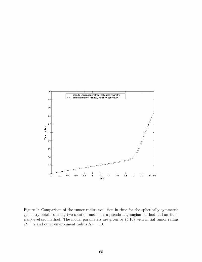
Figure 1: Comparison of the tumor radius evolution in time for the spherically symmetricgeometry obtained using two solution methods: a pseudo-Lagrangian method and an Eule-rian/level set method. The model parameters are given by (4.16) with initial tumor radiusR0 = 2 and outer environment radius RD = 10.

65

Fig

ure

2:E

volu

tion

ofth

etu

mor

radiu

sin

the

abse

nce

ofan

giog

enes

is.

The

solid

line

corr

espon

ds

to∆

D=

0.00

1an

dth

edas

hed

line

to∆

D=

1.T

he

rem

ainin

gm

odel

par

amet

ers

are

the

sam

eas

Fig

ure

1.A

stab

iliz

edst

ate

isap

pro

ached

for

∆D

=1.

66

Figure 3: Evolution of the tumor living cell density at various moments in time for sphericallysymmetric tumor growth (Figure 1 parameters). The first four curves correspond to theavascular phase of tumor growth, the fifth one to an intermediate (vascularization) phaseand the last two to a fully vascular phase.

67

Figure 4: Evolution of the tumor dead cell density at various moments in time for sphericallysymmetric tumor growth (Figure 1 parameters). Formation of a necrotic core in the centralregion of the tumor observed.

68

Figure 5: Evolution of the new capillary density at various moments in time for spheri-cally symmetric tumor growth (Figure 1 parameters). The endothelial cells stimulated toproliferate belong to the pre-existing capillary network, here located on the line segment7 ≤ r ≤ 8..

69

Figure 6: Evolution of the overall cell density inside the tumor at three moments in timefor spherically symmetric tumor growth (Figure 1 parameters). Development of increasinglysharp local gradients occurs.

70

Figure 7: Evolution of the tumor angiogenic factor (TAF) at various moments in time, inthe avascular and in the vascular phase of growth, for spherically symmetric tumor growth(Figure 1 parameters).

71

(a) avascular phase

(b) vascular phase

Figure 8: Nutrient evolution inside the tumor in the (a) avascular phase and in the (b)vascular phase of growth for spherically symmetric tumor growth (Figure 1 parameters).Nutrient levels are maximum at the tumor surface and gradually decreasing towards thecenter. 72

Figure 9: Comparison of the tumor radius evolution in time computed via three differentmethods: 2D Cartesian/narrow band level set method, 1D pseudo-Lagrangian method underthe assumption of polar symmetry and a 1D Eulerian/level set method under the assumptionof polar symmetry. The initial tumor boundary is a circle of center 0 and radius 1. Themodel parameters are given by (4.16), except that UC = 0.5 in the pre-existing capillaryregion.

73

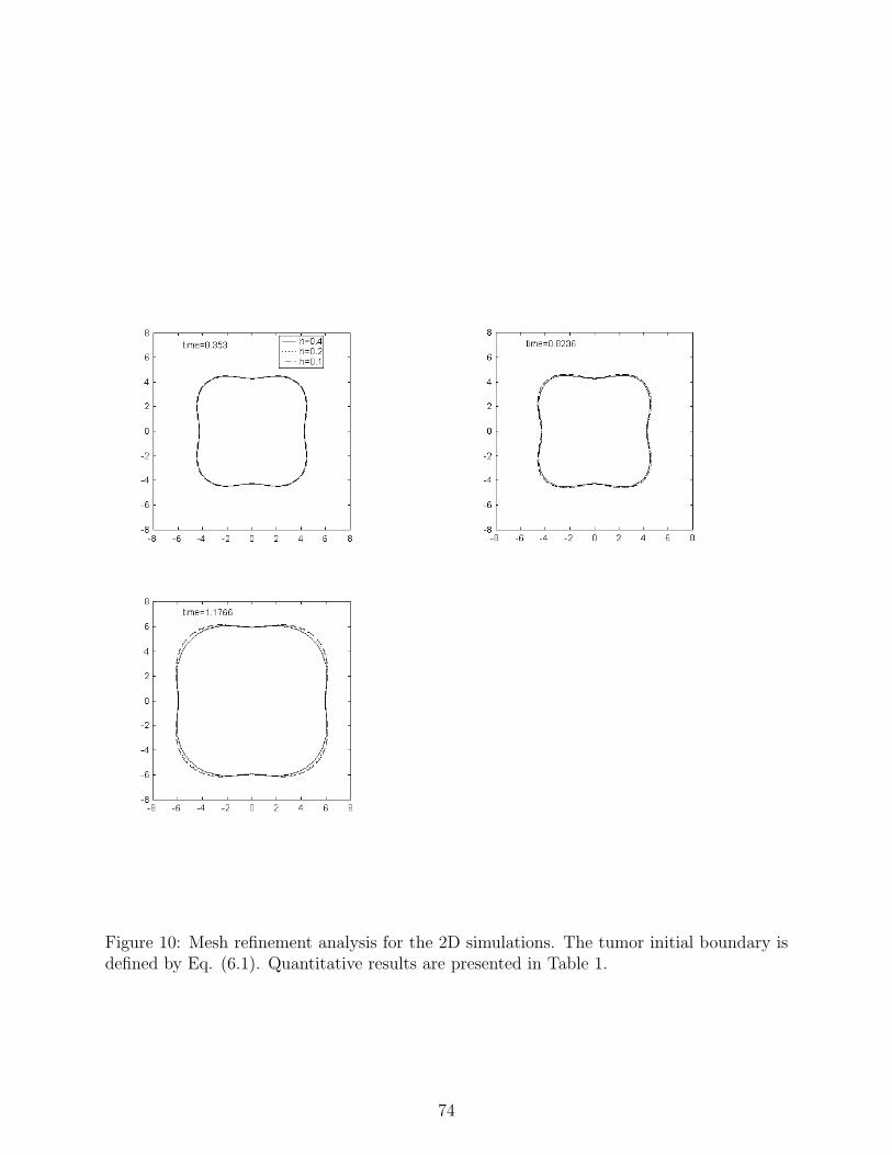
Figure 10: Mesh refinement analysis for the 2D simulations. The tumor initial boundary isdefined by Eq. (6.1). Quantitative results are presented in Table 1.

74

Figure 11(a): Evolution of the tumor in time, for the initial tumor boundary given byEq.(6.1). The four small circles outside of the initial tumor boundary correspond to thelocation of the pre-existing capillaries. The model parameters are the same as Figure 9.

75

Figure 11(b-1): Evolution of the new capillary density displayed as contour plots for theconditions of Figure 11(a).

76

Figure 11(b-2): Evolution of the new capillary density displayed as surface plots for theconditions of Figure 11(a).

77

Figure 11(c): Evolution of tumor living cell density displayed as contour plots for the con-ditions of Figure 11(a).

78

Figure 11(d): Evolution of tumor dead cell density displayed as contour plots for the condi-tions of Figure 11(a). The tendency to form a large necrotic region is observed.

79

Figure 11(e): Evolution of tumor angiogenic factor (TAF) displayed as contour plots for theconditions of Figure 11(a).

80

Figure 11(f): Evolution of nutrient concentration displayed as contour plots for the conditionsof Figure 11(a).

81

Figure 12(a): Evolution of the tumor in time, for the initial tumor boundary given byEq.(6.4). The initial size of the tumor and the overall domain have been scaled down by afactor of four. The four small circles outside of the initial tumor boundary correspond tothe location of the pre-existing capillaries. The model parameters are given by (4.16).

82

Figure 12(b-1): Evolution of the new capillary density displayed as contour plots for theconditions of Figure 12(a).

83

Figure 12(b-2): Evolution of the new capillary density displayed as surface plots for theconditions of Figure 12(a).

84

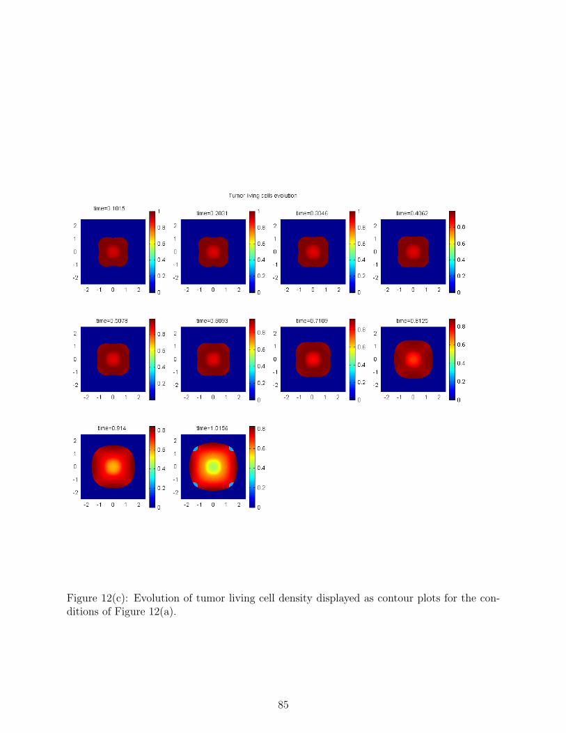
Figure 12(c): Evolution of tumor living cell density displayed as contour plots for the con-ditions of Figure 12(a).

85

Figure 12(d): Evolution of tumor dead cell density displayed as contour plots for the condi-tions of Figure 12(a). The tendency to form a large necrotic region is observed.

86

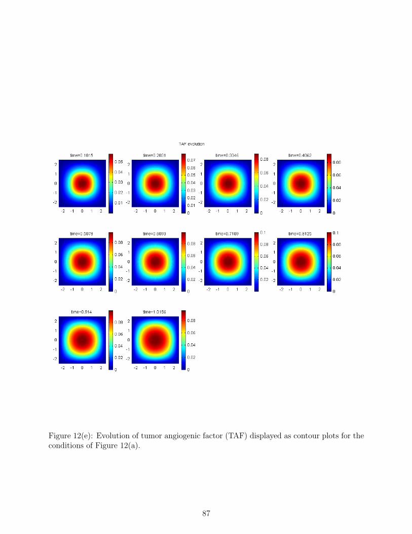
Figure 12(e): Evolution of tumor angiogenic factor (TAF) displayed as contour plots for theconditions of Figure 12(a).

87

Figure 12(f): Evolution of nutrient concentration displayed as contour plots for the conditionsof Figure 12(a).

88

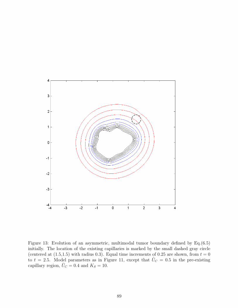
Figure 13: Evolution of an asymmetric, multimodal tumor boundary defined by Eq.(6.5)initially. The location of the existing capillaries is marked by the small dashed gray circle(centered at (1.5,1.5) with radius 0.3). Equal time increments of 0.25 are shown, from t = 0to t = 2.5. Model parameters as in Figure 11, except that UC = 0.5 in the pre-existingcapillary region, UC = 0.4 and KS = 10.

89

Figure 14: A comparison of the tumor boundary evolution for two model parameters char-acterizing the vascular phase of growth: KS and ΓC . The initial tumor boundary (same asFigure 13) is shown as the gray solid line. The tumor boundary at the final time t = 2.5 isshown as follows: KS = 10 and ΓC = 10, dotted line; KS = 0 and ΓC = 100, dash-dot line;KS = 10 and ΓC = 100, solid line.

90