Simulating competing risks data in survival analysis

STATISTICS IN MEDICINEStatist. Med. 2009; 28:956–971Published online 5 January 2009 in Wiley InterScience(www.interscience.wiley.com) DOI: 10.1002/sim.3516

Simulating competing risks data in survival analysis

Jan Beyersmann1,2,∗,†, Aurelien Latouche3, Anika Buchholz1,2

and Martin Schumacher2

1Freiburg Centre for Data Analysis and Modelling, University of Freiburg, Eckerstraße 1,79104 Freiburg, Germany

2Institute of Medical Biometry and Medical Informatics, University Medical Center Freiburg,Stefan-Meier-Straße 26, 79104 Freiburg, Germany

3Universite Versailles St–Quentin, EA 2506, Versailles, France

SUMMARY

Competing risks analysis considers time-to-first-event (‘survival time’) and the event type (‘cause’),possibly subject to right-censoring. The cause-, i.e. event-specific hazards, completely determine thecompeting risk process, but simulation studies often fall back on the much criticized latent failure timemodel. Cause-specific hazard-driven simulation appears to be the exception; if done, usually only constanthazards are considered, which will be unrealistic in many medical situations. We explain simulatingcompeting risks data based on possibly time-dependent cause-specific hazards. The simulation design is aseasy as any other, relies on identifiable quantities only and adds to our understanding of the competing risksprocess. In addition, it immediately generalizes to more complex multistate models. We apply the proposedsimulation design to computing the least false parameter of a misspecified proportional subdistributionhazard model, which is a research question of independent interest in competing risks. The simulationspecifications have been motivated by data on infectious complications in stem-cell transplanted patients,where results from cause-specific hazards analyses were difficult to interpret in terms of cumulative eventprobabilities. The simulation illustrates that results from a misspecified proportional subdistribution hazardanalysis can be interpreted as a time-averaged effect on the cumulative event probability scale. Copyrightq 2009 John Wiley & Sons, Ltd.

KEY WORDS: multistate model; cause-specific hazard; subdistribution hazard; latent failure time; modelmisspecification

∗Correspondence to: Jan Beyersmann, Freiburg Centre for Data Analysis and Modelling, University of Freiburg,Eckerstraße 1, 79104 Freiburg, Germany.

†E-mail: [email protected]

Contract/grant sponsor: Deutsche Forschungsgemeinschaft; contract/grant number: FOR 534

Received 21 April 2008Copyright q 2009 John Wiley & Sons, Ltd. Accepted 7 November 2008

SIMULATING COMPETING RISKS DATA 957

1. INTRODUCTION

Competing risks are an extension of classical survival analysis, where we observe one of a finitenumber of different event types (‘cause’) in addition to the time to the first event occurring(‘survival time’), possibly subject to right-censoring. Modern competing risks analysis is based onthe cause-, i.e. event-specific hazards, which are empirically identifiable and completely determinethe competing risks process [1–3]. However, simulation of competing risks data seldom appearsto be based on these key modelling quantities. Rather, the so-called latent failure time model [4] isused to generate data, where survival time and cause are modelled as arising from the minimum oflatent failure times corresponding to the different causes. This model has been heavily criticized forlack of plausibility in biomedical situations, but, even more importantly, for a non-identifiabilityproblem, as the dependence structure between the postulated latent failure times cannot be identifiedfrom the observable data [2, 3, 5, 6].

We found that 60 per cent of the articles published in Statistics in Medicine since 2000 that usedsimulations to study competing risks were built on the latent failure time model in order to generatedata. Only 12 per cent of the articles based their simulation designs on cause-specific hazards; allof these articles considered constant cause-specific hazards only, which will be unrealistic in manymedical situations. We found a similar picture for articles published in Biometrics, Biometrika,Lifetime Data Analysis and Computational Statistics and Data Analysis since 2000. Details of theliterature research are reported in Section 2.

The aim of this article is to explain how competing risks data can be simulated cause-specifichazards driven, where the hazards are allowed to be time-dependent. The simulation design is aseasy as any other, exactly reflects the way competing risks data are analysed, and being hazard-based, it corresponds to the way competing risks data occur over time. Unlike latent failuretime-based simulation, we will not need to specify unverifiable dependence structures.

A simulation design building on the fact that the cause-specific hazards completely determinethe distribution of competing risks data cannot be novel per se, but is an inherent part of thismathematical result. Presenting the algorithm, however, is relevant, as we will see from the literatureresearch that the one algorithm that builds on the same quantities as modern competing risksanalyses is hardly used.

As another fundamental strength, the simulation design generalizes straightforwardly to morecomplex multistate models [1, 7], e.g. to an illness–death model with recovery and possiblycompeting endpoints. As the number of transitions will be random in such a model, latent failuretime-based simulation will become difficult to tract analytically, but hazard-based simulation isstill straightforward. Such a model may also be used to simulate survival or competing risksdata conditional on time-dependent covariates, using a certain correspondence between discretecovariates and multistate models [8]. In fact, this algorithm has been mentioned as a side note ongenerating multistate bootstrap samples in a more theoretical article on transition probabilities ina Markov renewal model by Dabrowska [9], and this article is referred to in a recent article byFiocco et al. on reduced-rank Cox models in a multistate model [10]. We wish to note that thegeneral multistate algorithm also is an inherent part of the more general mathematical result that thetransition hazards completely determine the distribution of a multistate model [11, Theorem II.6.7],and that our approach to competing risks is based on multistate models.

As an example, we will use the recommended simulation design to study the least false parameter[12] of a misspecified proportional subdistribution hazards model, if, in fact, proportional cause-specific hazards models hold. This example will serve two purposes: First, it illustrates how

Copyright q 2009 John Wiley & Sons, Ltd. Statist. Med. 2009; 28:956–971DOI: 10.1002/sim

958 J. BEYERSMANN ET AL.

natural our proposed simulation design is, as it directly picks up from the quantities analysed inthe competing risks setting. Second, the simulation specifications have been chosen to illustratethe interpretational difficulties frequently encountered in competing risks, motivated by data oninfectious complications in stem-cell transplanted patients [13]. Proportional cause-specific hazardsmodelling is the standard regression model of choice, but results may be difficult to interpretin terms of the cumulative event probabilities. This difficulty has led to the development of theproportional subdistribution hazards model [14], which offers a synthesis of single cause-specifichazards analyses. In the absence of time-dependent covariates, this synthesis is interpretable interms of the cumulative event probability [15]. However, under a proportional cause-specific hazardsspecification, this model will be misspecified [16]. We illustrate that results from the model arestill useful as a time-averaged effect on the cumulative event probability scale [17].

The motivation for this study comes from applied medical research: The aforementioned inter-pretational difficulties have led to results from both cause-specific hazards analyses and fromsubdistribution hazards analyses being reported side by side. Examples come, among other fields,from cancer [18], AIDS [19] and also the methodological literature [20]. As proportional cause-specific and proportional subdistribution hazards models preclude one another, at least one approachimplicitly reports a time-averaged effect. In our simulations, we have assumed the proportionalcause-specific hazards models to be correctly specified, as the competing risks situation does notimpose any further theoretical restrictions on these models. In contrast, assuming proportionalsubdistribution hazards models restricts the regression coefficient from one model given the regres-sion coefficient from the competing subdistribution model. Hence, it seemed natural to view thesubdistribution analysis as a time-averaged synthesis.

The aim of our simulation is twofold: First, we will use simulations to numerically approximatethe least false parameter, i.e. the time-averaged synthesis, as the least false parameter is onlyimplicitly given. Second, we will investigate how well the least false parameter may be estimated ina concrete study setting. These results are of independent interest, given the fact that the proportionalsubdistribution hazards model has attracted quite some interest recently, see in addition [21–25].We note that using simulation for numerical approximation, if a consistent estimate is available,is a classical textbook example, e.g. [26, Chapter I].

The article is organized as follows: The results of our literature research are given in Section 2.Section 3 introduces the competing risks multistate model and the cause-specific hazards-basedsimulation design. Example and Discussion are in Sections 4 and 5, respectively. We also describea cause-specific hazards-driven algorithm to generate competing risks data following a proportionalsubdistribution hazards model in the Appendix; this algorithm appears to be new to the literature.

We note that Section 3 introduces the distinct causes of failure as values of exactly one randomvariable, such that the question of dependent or independent competing risks does not apply. Also,introduction of the subdistribution hazard framework and the notion of the least false parameteras well as illustration of the interpretational difficulties that often come with competing risks dataare deferred to Section 4. Both Sections 3 and 4 emphasize the interpretational aspect, as it mayhave been the difficulties inherent to competing risks data that have led to simulations being basedon latent failure times in the past, without, of course, solving these difficulties.

For ease of presentation, we consider a competing risks model with two competing events only.The simulation design straightforwardly extends to more than two competing risks, as indicated inSection 3. The analysis of the least false parameter in Section 4 is not affected by the restrictionto two competing risks, as the subdistribution hazards model analyses one event of interest, andall other risks may be subsumed into one competing event.



We will write CSH for cause-specific hazard, SH for subdistribution hazard and CIF for thecumulative incidence function, i.e. the expected proportion of individuals experiencing a certainevent as time progresses, in the following.

2. RESULTS OF THE LITERATURE RESEARCH

We first conducted a literature research in Statistics in Medicine using the journal’s web pagehttp://www3.interscience.wiley.com/cgi-bin/jhome/2988/, last accessed onSeptember 24th, 2008. We found 60 articles that featured the term ‘competing risk’ or ‘competingrisks’ in the title and/or in the key words. Twenty-six (43.3 per cent of 60) articles used simulationstudies, 25 of these have been published after and including the year 2000. Fifteen (57.7 per centof 26) articles based their simulation design on the latent failure time approach. A surprisinglysmall number of only four (15.4 per cent) [27–30] articles generated data CSH-driven; however,all four articles used constant hazard models only. While constant hazard models are the easiestand therefore the best understood, they will be unrealistic in many medical situations. Still, Benderet al. [31] argue in a recent Statistics in Medicine article on survival times simulation that time-dependent hazards ‘seem to be underutilized’. Three (11.5 per cent) articles [32–34] simulateddata by first deciding how many individuals fail from each competing event at all and subsequentlysimulating the survival time conditional on the cause. Finally, four (15.4 per cent) articles workedin the SH setting and applied the simulation design used by the originators of the proportional SHmodel [14]; here, due to the very nature of the model, survival times are generated such that thecorresponding distribution function has mass at infinity. The algorithm in [14] generated failuretimes of one event type from a subdistribution (with mass at infinity) and failure times of thecompeting events conditional on the cause. The algorithm is therefore related to the one used in[32–34]. In Appendix A.1, we present a CSH-driven algorithm than simulates competing risksdata from a proportional SH model.

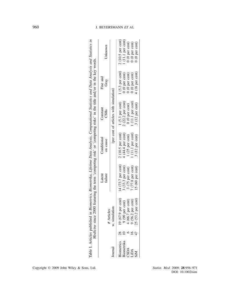
Next, we extended the literature search to Biometrics, Biometrika, Lifetime Data Analysis andComputational Statistics and Data Analysis. We decided to concentrate the search on articlespublished since (and including) 2000, as the initial literature search in Statistics in Medicine hadindicated this to be a relevant time interval. Also, focusing on articles published since 2000 shouldfavour models based on counting processes and, hence, hazards instead of latent failure times.Details of the extended review are given in Table I. For comparison, we have also reported therespective results for articles published in Statistics in Medicine since 2000. Overall, the extendedreview confirmed the picture of the initial literature search. We could not identify the simulationalgorithm for two articles [35, 36] published in Biometrics and for one article [37] published inBiometrika; reference [35] considered competing risks data to arise from latent failure times. OneBiometrics article [38] and one Biometrika article [39] generated data both conditional on thecause and from latent times.

3. COMPETING RISKS

3.1. The model

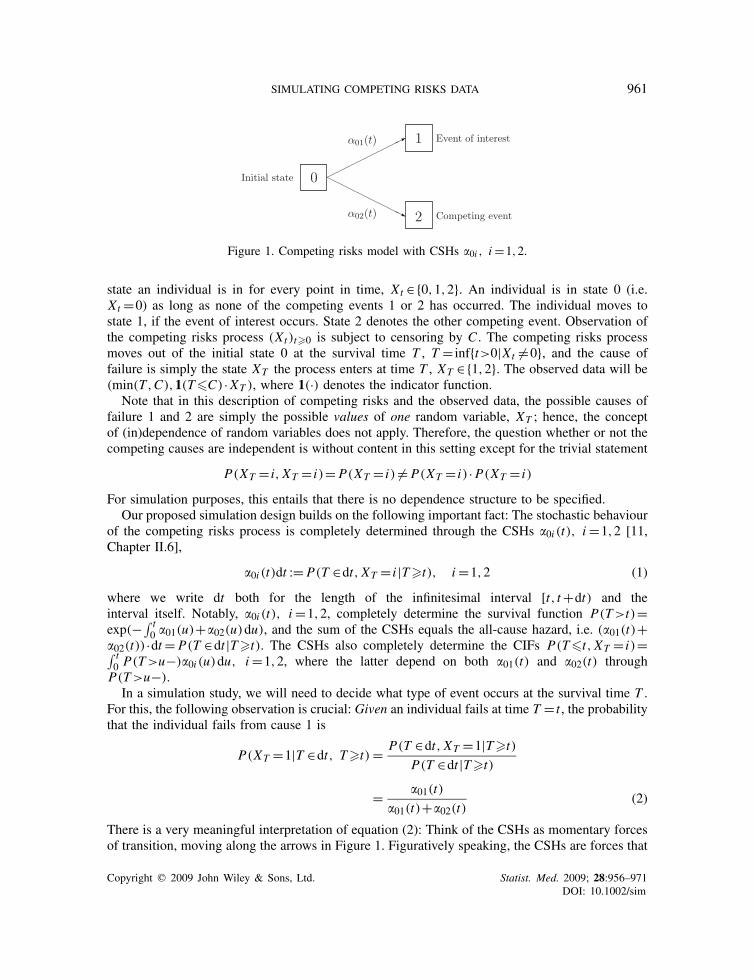
Following, e.g. [1; 2, Chapter 8.3; 3; 11, Chapter IV.4], we model competing risks as a multistateprocess, see also [40]: Consider the competing risks process (Xt )t�0 of Figure 1, denoting the



TableI.Articlespublishedin

Biometrics,Biometrika,LifetimeDataAnalysis,Com

putational

Statistics

andDataAnalysisandStatistics

inMedicinesince2000

featuringtheterm

‘com

petin

grisk’or

‘com

petin

grisks’

inthetitle

and/or

inthekeywords.

Latent

Con

ditio

nal

Con

stant

Fine

and

failu

reon

cause

CSH

sGray

Unk

nown

#Articles

Journal

w.simulation

(per

cent

ofartic

leswith

simulation)

Biometrics

2819

(67.9percent)

14(73.7percent)

2(10.5percent)

1(5.3

percent)

1(5.3

percent)

2(10.5percent)

Biometrika

109(90percent)

3(33.3percent)

4(44.4percent)

2(22.2percent)

0(0

percent)

1(11.1percent)

CSD

A6

4(66.7percent)

3(75percent)

1(25percent)

0(0

percent)

0(0

percent)

0(0

percent)

LiDA

169(56.2percent)

7(77.8percent)

1(11.1percent)

1(11.1percent)

0(0

percent)

0(0

percent)

SiM

4725

(53.2percent)

15(60percent)

3(12percent)

3(12percent)

4(16percent)

0(0

percent)



Figure 1. Competing risks model with CSHs �0i , i=1,2.

state an individual is in for every point in time, Xt ∈{0,1,2}. An individual is in state 0 (i.e.Xt =0) as long as none of the competing events 1 or 2 has occurred. The individual moves tostate 1, if the event of interest occurs. State 2 denotes the other competing event. Observation ofthe competing risks process (Xt )t�0 is subject to censoring by C . The competing risks processmoves out of the initial state 0 at the survival time T , T = inf{t>0|Xt �=0}, and the cause offailure is simply the state XT the process enters at time T , XT ∈{1,2}. The observed data will be(min(T,C),1(T�C) ·XT ), where 1(·) denotes the indicator function.

Note that in this description of competing risks and the observed data, the possible causes offailure 1 and 2 are simply the possible values of one random variable, XT ; hence, the conceptof (in)dependence of random variables does not apply. Therefore, the question whether or not thecompeting causes are independent is without content in this setting except for the trivial statement

P(XT = i, XT = i)= P(XT = i) �= P(XT = i) ·P(XT = i)

For simulation purposes, this entails that there is no dependence structure to be specified.Our proposed simulation design builds on the following important fact: The stochastic behaviour

of the competing risks process is completely determined through the CSHs �0i (t), i=1,2 [11,Chapter II.6],

�0i (t)dt := P(T ∈dt, XT = i |T�t), i=1,2 (1)

where we write dt both for the length of the infinitesimal interval [t, t+dt) and theinterval itself. Notably, �0i (t), i=1,2, completely determine the survival function P(T>t)=exp(−∫ t

0 �01(u)+�02(u)du), and the sum of the CSHs equals the all-cause hazard, i.e. (�01(t)+�02(t)) ·dt= P(T ∈dt |T�t). The CSHs also completely determine the CIFs P(T�t, XT = i)=∫ t0 P(T>u−)�0i (u)du, i=1,2, where the latter depend on both �01(t) and �02(t) throughP(T>u−).In a simulation study, we will need to decide what type of event occurs at the survival time T .

For this, the following observation is crucial: Given an individual fails at time T = t , the probabilitythat the individual fails from cause 1 is

P(XT =1|T ∈dt, T�t) = P(T ∈dt, XT =1|T�t)

P(T ∈dt |T�t)

= �01(t)

�01(t)+�02(t)(2)

There is a very meaningful interpretation of equation (2): Think of the CSHs as momentary forcesof transition, moving along the arrows in Figure 1. Figuratively speaking, the CSHs are forces that



draw an individual out of the initial state 0 and towards the competing risks states. Assuming thatan individual fails at time T = t , the probability that the failure cause is 1 equals the proportionthat the CSH for failure 1 at time t contributes to the all-cause hazard �01(t)+�02(t), which drawsat the individual. (An analogous interpretation holds for the factors of the partial likelihood in aCox model [41, 42].)

We have formulated the competing risks process in continuous time, but it is worth pointingout that this formulation transfers to discrete time by simply putting [11, p. 94]

�0i (t)= P(Xt = i |T�t), i=1,2 (3)

3.2. The simulation design

Again, we refer to the recent excellent articles by Burton et al. [43] on planning simulation studies(including some material on survival data) and by Bender et al. [31] on more specific survivalissues.

As claimed above, simulating competing risks data CSH-driven now (with the framework ofSection 3.1) is easy:

1. Specify the CSHs �01(t) and �02(t) as functions of time, possibly depending on covariatevalues [31].

2. Simulate survival times T with all-cause hazard �01(t)+�02(t).3. For a simulated survival time T run a binomial experiment, which decides with probability

�01(T )/(�01(T )+�02(T )) on cause 1.4. Additionally (and as usual with survival data), generate censoring times C .

If we wish to simulate competing risks data with more than two competing event states, we willneed to substitute the binomial experiment of step 3 by a multinomial experiment.

4. EXAMPLE

This section is organized as follows: In Section 4.1 we specify proportional CSH models with abinary covariate. The motivation for this model specification is given in Section 4.2. We will findthat the effect of the covariate on the CIFs is difficult to tell from the CSH models, which leads usto considering proportional SH models explained in Section 4.3. However, proportional SHs willin general not hold, if proportional CSHs hold. Still, results from a proportional SHs analysis aremeaningful in terms of the least false parameter, a time-averaged effect (Section 4.4). While theleast false parameter is hard to tract analytically, we can easily approximate it through simulations.This is done in Section 4.5. Finally, a second simulation study is reported in Section 4.6, wherewe investigate how well the least false parameter may be estimated in a concrete study setting.

4.1. Model specification

Consider the following specification of a competing risks model:

�01;Z=0(t)= 0.09

t+1and �02;Z=0(t)=0.024 ·t (4)



Time t

0 10 20 30 40 50 60 70

0.00

0.01

0.02

0.03

0.04

0.05

0.06

Z=0Z=1

Time tS

ubdi

strib

utio

n ha

zard

Cau

se–s

peci

fic h

azar

d

0 10 20 30 40 50 60 70

0.00

0.01

0.02

0.03

0.04

0.05

0.06

Z=0Z=1

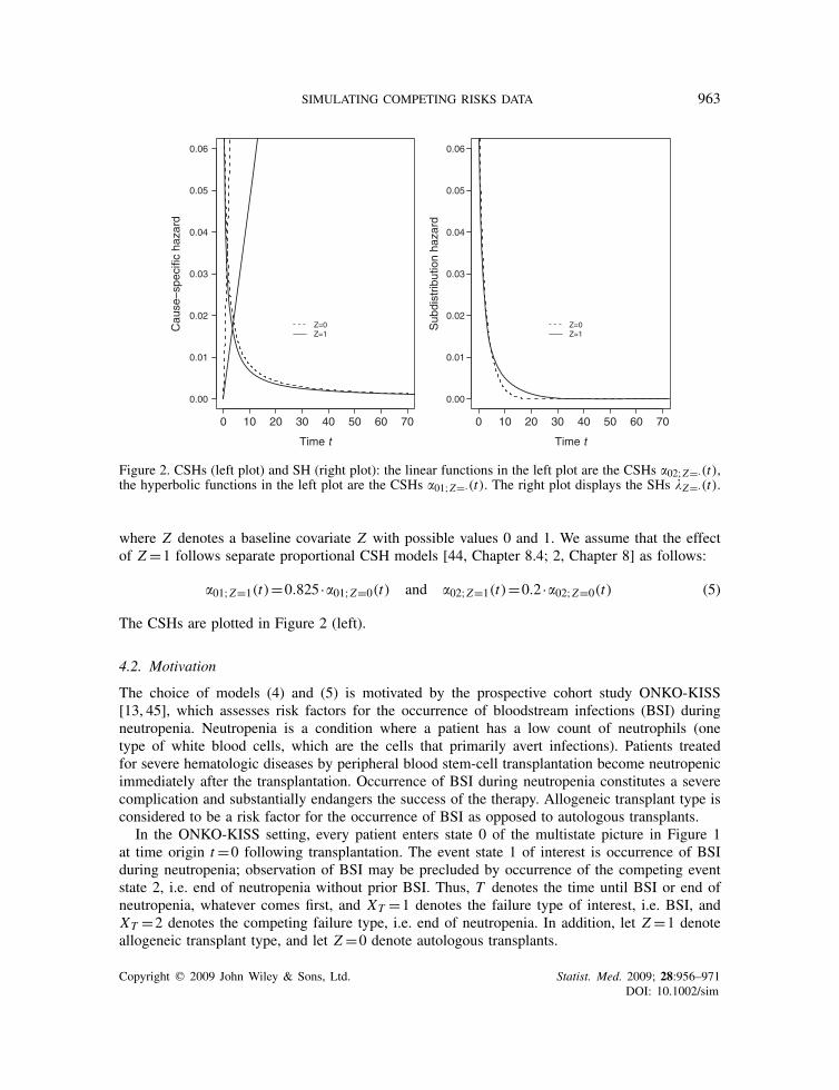
Figure 2. CSHs (left plot) and SH (right plot): the linear functions in the left plot are the CSHs �02;Z=·(t),the hyperbolic functions in the left plot are the CSHs �01;Z=·(t). The right plot displays the SHs �Z=·(t).

where Z denotes a baseline covariate Z with possible values 0 and 1. We assume that the effectof Z =1 follows separate proportional CSH models [44, Chapter 8.4; 2, Chapter 8] as follows:

�01;Z=1(t)=0.825 ·�01;Z=0(t) and �02;Z=1(t)=0.2 ·�02;Z=0(t) (5)

The CSHs are plotted in Figure 2 (left).

4.2. Motivation

The choice of models (4) and (5) is motivated by the prospective cohort study ONKO-KISS[13, 45], which assesses risk factors for the occurrence of bloodstream infections (BSI) duringneutropenia. Neutropenia is a condition where a patient has a low count of neutrophils (onetype of white blood cells, which are the cells that primarily avert infections). Patients treatedfor severe hematologic diseases by peripheral blood stem-cell transplantation become neutropenicimmediately after the transplantation. Occurrence of BSI during neutropenia constitutes a severecomplication and substantially endangers the success of the therapy. Allogeneic transplant type isconsidered to be a risk factor for the occurrence of BSI as opposed to autologous transplants.

In the ONKO-KISS setting, every patient enters state 0 of the multistate picture in Figure 1at time origin t=0 following transplantation. The event state 1 of interest is occurrence of BSIduring neutropenia; observation of BSI may be precluded by occurrence of the competing eventstate 2, i.e. end of neutropenia without prior BSI. Thus, T denotes the time until BSI or end ofneutropenia, whatever comes first, and XT =1 denotes the failure type of interest, i.e. BSI, andXT =2 denotes the competing failure type, i.e. end of neutropenia. In addition, let Z =1 denoteallogeneic transplant type, and let Z =0 denote autologous transplants.



Time t

0 10 20 30 40 50 60 70

0.0

autologous (Z=0)allogeneic (Z=1)

CIF

for

the

occu

rren

ce o

f BS

I

Time t

0 10 20 30 40 50 60 70C

IF fo

r th

e co

mpe

ting

even

t

autologous (Z=0)allogeneic (Z=1)

0.1

0.2

0.3

0.4

0.5

0.6

0.7

0.8

0.9

1.0

0.0

0.1

0.2

0.3

0.4

0.5

0.6

0.7

0.8

0.9

1.0

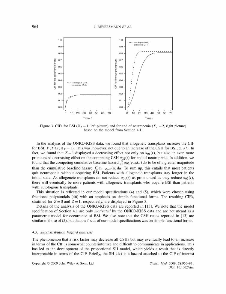
Figure 3. CIFs for BSI (XT =1, left picture) and for end of neutropenia (XT =2, right picture)based on the model from Section 4.1.

In the analysis of the ONKO-KISS data, we found that allogeneic transplants increase the CIFfor BSI, P(T�t, XT =1). This was, however, not due to an increase of the CSH for BSI, �01(t). Infact, we found that Z =1 displayed a decreasing effect not only on �01(t), but also an even morepronounced decreasing effect on the competing CSH �02(t) for end of neutropenia. In addition, wefound that the competing cumulative baseline hazard

∫ t0 �02;Z=0(u)du to be of a greater magnitude

than the cumulative baseline hazard∫ t0 �01;Z=0(u)du. To sum up, this entails that most patients

quit neutropenia without acquiring BSI. Patients with allogeneic transplants stay longer in theinitial state. As allogeneic transplants do not reduce �01(t) as pronounced as they reduce �02(t),there will eventually be more patients with allogeneic transplants who acquire BSI than patientswith autologous transplants.

This situation is reflected in our model specifications (4) and (5), which were chosen usingfractional polynomials [46] with an emphasis on simple functional forms. The resulting CIFs,stratified for Z =0 and Z =1, respectively, are displayed in Figure 3.

Details of the analysis of the ONKO-KISS data are reported in [13]. We note that the modelspecification of Section 4.1 are only motivated by the ONKO-KISS data and are not meant as aparametric model for occurrence of BSI. We also note that the CSH ratios reported in [13] aresimilar to those of (5), but that the focus of our model specifications was on simple functional forms.

4.3. Subdistribution hazard analysis

The phenomenon that a risk factor may decrease all CSHs but may eventually lead to an increasein terms of the CIF is somewhat counterintuitive and difficult to communicate in applications. Thishas led to the development of the proportional SH model, which yields a result that is directlyinterpretable in terms of the CIF. Briefly, the SH �(t) is a hazard attached to the CIF of interest



Time t

Sub

dist

ribut

ion

haza

rd r

atio

0 1 2 3 4 5 6 7 8 9 10

0.00

λZ=1(t) λZ=0(t)

exp(β~)

0.50

1.00

1.50

2.00

2.50

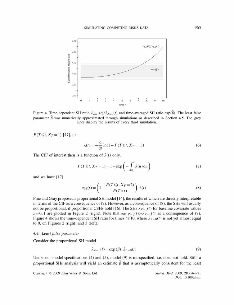
Figure 4. Time-dependent SH ratio �Z=1(t)/�Z=0(t) and time-averaged SH ratio exp(�). The least falseparameter � was numerically approximated through simulations as described in Section 4.5. The grey

lines display the results of every third simulation.

P(T�t, XT =1) [47], i.e.

�(t)=− d

dtln(1−P(T�t, XT =1)) (6)

The CIF of interest then is a function of �(t) only,

P(T�t, XT =1)=1−exp

(−

∫ t

0�(u)du

)(7)

and we have [17]

�01(t)=(1+ P(T�t, XT =2)

P(T>t)

)·�(t) (8)

Fine and Gray proposed a proportional SH model [14], the results of which are directly interpretablein terms of the CIF as a consequence of (7). However, as a consequence of (8), the SHs will usuallynot be proportional, if proportional CSHs hold [16]. The SHs �Z=z(t) for baseline covariate valuesz=0,1 are plotted in Figure 2 (right). Note that �01;Z=z(t)>�Z=z(t) as a consequence of (8).Figure 4 shows the time-dependent SH ratio for times t�10, where �Z=0(t) is not yet almost equalto 0, cf. Figures 2 (right) and 3 (left).

4.4. Least false parameter

Consider the proportional SH model

�Z=1(t)=exp(�) ·�Z=0(t) (9)

Under our model specifications (4) and (5), model (9) is misspecified, i.e. does not hold. Still, aproportional SHs analysis will yield an estimate � that is asymptotically consistent for the least



false parameter � (which is unequal �) [12, 48]. We can interpret exp(�) as a time-averaged subdis-tribution hazard ratio. However, � is analytically hardly tractable. But as � is an asymptoticallyconsistent estimate of �, we can approximate the least false parameter through simulations. Theapproximation is reported in the following subsection.

4.5. Simulation study I

The aim of this subsection is to numerically approximate the least false parameter �, using the factthat it is asymptotically consistently estimated by �. See e.g. [26, Chapter I] on using simulationfor numerical approximation. Simulations were done with R [49]. Survival times T were generatedvia the inversion method, using the R-function uniroot() for numerical inversion. On the basisof the ONKO-KISS study, we set P(Z =1)=0.565. We decided to perform each simulation with10 000 individuals, as the aim of the present simulation was to numerically approximate the leastfalse parameter rather than to mimic a particular study setting with probably a smaller number ofindividuals. We used the following stop criterion: We first ran 100 simulations and then appliedthe following stepwise procedure:

1. We computed the arithmetic mean of the results from the proportional SH analysis.2. We added 100 new simulations and updated the arithmetic mean.3. If the updated mean differed from the previous value by more than 0.1 per cent, we added

another 100 simulations and so forth. Otherwise, the procedure stopped.

Using this criterion, we stopped after 500 simulations. The least false parameter � was approxi-mately equal to 0.085. The time-averaged SH ratio exp(�)≈1.09 is illustrated in Figure 4 alongwith results from every third simulation. Based on the 500 simulations, the empirical standarderror was estimated as 0.007. An asymptotic 95 per cent-confidence interval for exp(�) based onnormal approximation [12] is then [1.07,1.10].

Interpreting exp(�) as a time-averaged SH ratio, this result indicates a slight increase of the CIFfor BSI for patients with allogeneic transplants, which is in line with Figures 3 and 4.

4.6. Simulation study II

The aim of this subsection is to investigate how well the least false parameter may be estimatedin a setting like in the original ONKO-KISS study. For simplicity, we decided to compute 1000simulations. Each simulation comprised 1616 individuals as in the original ONKO-KISS analysis[45]. In each simulation, we performed a proportional SH analysis and recorded the point estimate �and its model-based variance estimator var(�). We compared the point estimates with the numericalapproximation obtained in the previous subsection, and we also compared the model-based varianceestimator with the empirical variance obtained from the point estimates in the 1000 simulations.

Finally, we studied the coverage of the confidence intervals �±q0.975 ·√var(�), where q0.975≈1.96

is the 0.975-quantile of the standard normal distribution.The estimate � of the least false parameter was on average 0.90, corresponding to a time-

averaged SH ratio estimate of exp(�)≈1.09. The model-based variance estimator var(�) was onaverage 0.0145 and the empirical variance of � was 0.0143. The coverage of the model-based 95per cent-confidence intervals was 95.3 per cent.



5. DISCUSSION

We have presented a design for simulating competing risks data, which is as easy as any other,but relies on those identifiable quantities only, which form the basis of modern competing risksstatistics. As a consequence, the proposed simulation design adds to our understanding of thecompeting risks process, which we have demonstrated computing the least false parameter of amisspecified proportional SH model, if proportional CSH models hold.

We should note that simulating the failure cause for competing risks data using the predominantlatent failure time model is not wrong, although opposed to understanding what CSHs do; inparticular, the identifiability problem of the latent failure time model implies that we may useindependent latent times to generate the data, as we cannot tell the dependency structure fromwhat is being observed. However, the notorious question of the dependency structure is renderedsuperfluous with the CSH-based simulation design. In this context, we also note that the proposedsimulation design passes the test of Occam’s razor (e.g. [50, p. 435]), while the latent failuretime-based one usually does not.

Another advantage of the proposed simulation design is that it immediately generalizes to morecomplex multistate models with a random number of transitions, see also [9]. Here, we would notknow the ‘reservoir’ of latent times needed for simulation, but transition hazard-based simulationis straightforward through a series of competing risks-type experiments. This is, e.g. of interestfor simulating time-dependent covariates [8], a current research topic [51].

A further worthwhile topic of future research is studying the type of CSH models that giverise to a proportional SH model based on the CSH-driven simulation algorithm for proportionalSH model data that we have given in the Appendix and that appears to be new to the literature.However, such work has been beyond the scope of the present manuscript.

In closing, we comment on a number of issues regarding our example: Using the concept ofthe least false parameter, we heavily borrowed from Hjort’s ‘agnostic point of view’ towardsmodel assumptions [12]: For a concrete data analysis, this would entail that one would not claim aproportional effect of a covariate on the SH (or on the CSHs, for that matter). But one would profitfrom the simple structure of a proportional hazards model in that the results display an averageeffect on the SH (or CSH) scale. If one is willing to take this agnostic point of view, the aim ofthe analysis would be a synthesis analysis, potentially first on the CSH scale, then (in a furthersummarizing step) on the SH, i.e. on the CIF scale.

The results from the second simulation study in Section 4.6 show that such a summary analysis isfeasible in a concrete study setting and under an interpretationally challenging CSH constellation.Significance, however, is a different and quite subtle issue: In the original data analysis, we foundsignificant effects on the CSHs (reflected in (5)), leading to crossing CIFs (as in Figure 3, left) andan least false parameter, which should presumably be somewhat larger than zero (as approximatedin Section 4.5). However, in such a situation, we cannot necessarily expect the estimate of theleast false parameter to be significantly different from zero; for the original ONKO-KISS data,we found a time-averaged SH ratio 1.1([0.89,1.4]) [13, Table I]. The variance estimates fromthe second simulation study confirm that significance of the least false parameter estimate is yetanother issue under the given CSH constellation. If the aim of the analysis is to verify that theCIFs cross, confidence bands should be studied [27].

While the summarizing approach in terms of the least false parameter is useful, it does notdispose of model choice considerations. This is, e.g. a concern, if the aim of the analysis isprediction [52] or studying time-varying effects [53]. A further issue inherent to competing risks



is that proportional cause-specific and proportional all-cause hazards models preclude one another,since the all-cause hazard is the sum of all CSHs. This is a concern for hazard-based modelling;Klein [54] therefore argued in favour of Aalen’s additive hazard model [11, Chapter VII.4].

We also wish to note that the model specification of Section 4.1 is not meant as a parametricmodel for occurrence of BSI during neutropenia for, say, prediction purposes. Rather, our aim wasto illustrate the usefulness of the proposed simulation design in a specific competing risks setting,motivated by a concrete data example, but with the emphasis on simple functional form. Wehave also refrained from simulating censoring times, which is easy and as with standard survivalsimulation. Our example has also been meant to illustrate the special difficulties encountered incompeting risks as well as the relative merits of CSH- and SH-based analyses, respectively. Wenote that, in a concrete data analysis, the least false parameter of a misspecified SH model (or ofa misspecified CSH model) may also be approximated using the bootstrap on the data at hand.

APPENDIX A

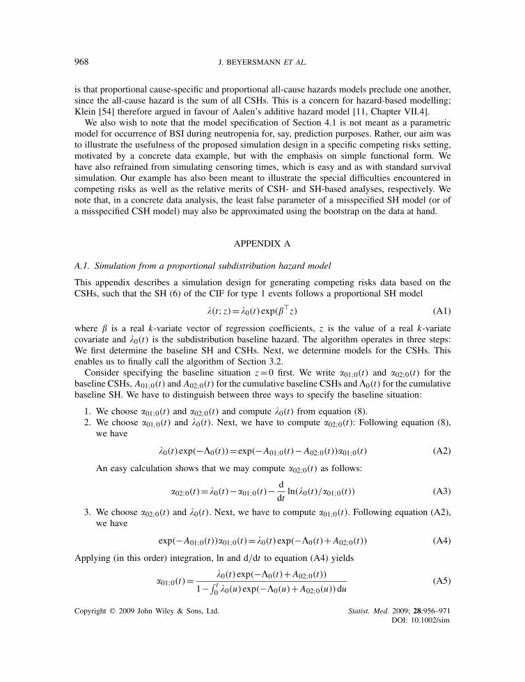
A.1. Simulation from a proportional subdistribution hazard model

This appendix describes a simulation design for generating competing risks data based on theCSHs, such that the SH (6) of the CIF for type 1 events follows a proportional SH model

�(t; z)=�0(t)exp(��z) (A1)

where � is a real k-variate vector of regression coefficients, z is the value of a real k-variatecovariate and �0(t) is the subdistribution baseline hazard. The algorithm operates in three steps:We first determine the baseline SH and CSHs. Next, we determine models for the CSHs. Thisenables us to finally call the algorithm of Section 3.2.

Consider specifying the baseline situation z=0 first. We write �01;0(t) and �02;0(t) for thebaseline CSHs, A01;0(t) and A02;0(t) for the cumulative baseline CSHs and�0(t) for the cumulativebaseline SH. We have to distinguish between three ways to specify the baseline situation:

1. We choose �01;0(t) and �02;0(t) and compute �0(t) from equation (8).2. We choose �01;0(t) and �0(t). Next, we have to compute �02;0(t): Following equation (8),

we have

�0(t)exp(−�0(t))=exp(−A01;0(t)−A02;0(t))�01;0(t) (A2)

An easy calculation shows that we may compute �02;0(t) as follows:

�02;0(t)=�0(t)−�01;0(t)− d

dtln(�0(t)/�01;0(t)) (A3)

3. We choose �02;0(t) and �0(t). Next, we have to compute �01;0(t). Following equation (A2),we have

exp(−A01;0(t))�01;0(t)=�0(t)exp(−�0(t)+A02;0(t)) (A4)

Applying (in this order) integration, ln and d/dt to equation (A4) yields

�01;0(t)= �0(t)exp(−�0(t)+A02;0(t))1−∫ t

0 �0(u)exp(−�0(u)+A02;0(u))du(A5)



In the second step, we need to specify CSH models �01(t; z) and �02(t; z) given the baselineCSHs and SH, such that model (A1) holds. We choose either a model �01(t; z) or a model�02(t; z). This could be, e.g. a Cox model, but may also be some other model, say an additive CSHmodel [54]. We have to distinguish two situations: If we choose a model �01(t; z), we determinethe model �02(t; z) as in equation (A3), i.e.

�02(t; z)=�(t; z)−�01(t; z)− d

dtln(�(t; z)/�01(t; z)) (A6)

If, however, we choose a model �02(t; z), we determine the model �01(t; z) as in equation (A5), i.e.

�01(t; z)= �(t; z)exp(−�(t; z)+A02(t; z))1−∫ t

0 �(u; z)exp(−�(u; z)+A02(u; z))du (A7)

In the third and final step, we can now use the algorithm of Section 3.2.In practice, one will usually first determine the baseline CSHs, which can essentially be any ‘well

behaving’ (differentiable, integrable) non-negative function, whereas choice of �0(t) is compli-cated by the fact that 1− limt→∞ exp(−�0(t))= P(XT =1|Z =0). Next, specifying models (A1)and �01(t; z) and using equation (A6) is the most convenient option. Note that equations (A3),(A5)–(A7) are subject to the constraint that they result in non-negative functions.

REFERENCES

1. Putter H, Fiocco R, Geskus R. Tutorial in biostatistics: competing risks and multi-state models. Statistics inMedicine 2007; 26(11):2277–2432.

2. Kalbfleisch JD. The Statistical Analysis of Failure Time Data. Wiley: New York, 2002.3. Andersen P, Abildstrøm S, Rosthøj S. Competing risks as a multi-state model. Statistical Methods in Medical

Research 2002; 11(2):203–215.4. David H, Moeschberger M. The Theory of Competing Risks. Griffin’s Statistical Monograph No. 39. Macmillan:

New York, 1978.5. Tsiatis A. A nonidentifiability aspect of the problem of competing risks. Proceedings of the National Academy

of Sciences U.S.A. 1975; 72:20–22.6. Prentice R, Kalbfleisch J, Peterson A, Flournoy N, Farewell V, Breslow N. The analysis of failure times in the

presence of competing risks. Biometrics 1978; 34:541–554.7. Andersen P, Keiding N. Multi-state models for event history analysis. Statistical Methods in Medical Research

2002; 11(2):91–115.8. Andersen PK. Time-dependent covariates and Markov processes. In Modern Statistical Methods in Chronic

Disease Epidemiology, Moolgavkar SH, Prentice RL (eds). Wiley: New York, 1986; 82–103.9. Dabrowska DM. Estimation of transition probabilities and bootstrap in a semiparametric Markov renewal model.

Journal of Nonparametric Statistics 1995; 5:237–259.10. Fiocco M, Putter H, van Houwelingen H. Reduced-rank proportional hazards regression and simulation-based

prediction for multi-state models. Statistics in Medicine 2008; DOI: 10.1002/sim.2712.11. Andersen P, Borgan Ø, Gill RD, Keiding N. Statistical Models Based on Counting Processes. Springer Series in

Statistics. Springer: New York, NY, 1993.12. Hjort NL. On inference in parametric survival data models. International Statistical Review 1992; 60:355–387.13. Beyersmann J, Dettenkofer M, Bertz H, Schumacher M. A competing risks analysis of bloodstream infection

after stem-cell transplantation using subdistribution hazards and cause-specific hazards. Statistics in Medicine2007; 26(30):5360–5369.

14. Fine J, Gray RJ. A proportional hazards model for the subdistribution of a competing risk. Journal of theAmerican Statistical Association 1999; 94(446):496–509.

15. Beyersmann J, Schumacher M. Time-dependent covariates in the proportional subdistribution hazards model forcompeting risks. Biostatistics 2008; 9:765–776. DOI: 10.1093/biostatistics/kxn009.



16. Latouche A, Boisson V, Porcher R, Chevret S. Misspecified regression model for the subdistribution hazard ofa competing risk. Statistics in Medicine 2007; 26(5):965–974.

17. Beyersmann J, Schumacher M. Letter to the editor: comment on ‘A. Latouche, V. Boisson, and R. Porcher,S. Chevret: misspecified regression model for the subdistribution hazard of a competing risk, Statistics in Medicine,2006, DOI: 10.2002/sim.2600’. Statistics in Medicine 2007; 26(7):1649–1651.

18. Milosevic M, Fyles A, Hedley D, Pintilie M, Levin W, Manchul L, Hill R. Interstitial fluid pressure predictssurvival in patients with cervix cancer independent of clinical prognostic factors and tumor oxygen measurements.Cancer Research 2001; 61(17):6400–6405.

19. del Amo J, Perez-Hoyos S, Moreno A, Quintana M, Ruiz I, Cisneros J, Ferreros I, Gonzalez C, de Olalla PG,Perez R, Hernandez I. Trends in AIDS and mortality in HIV-infected subjects with hemophilia from 1985 to2003: the competing risks for death between AIDS and liver disease. Journal of Acquired Immune DeficiencySyndromes 2006; 41(5):624–631.

20. Zhang MJ, Fine J. Summarizing differences in cumulative incidence functions. Statistics in Medicine 2008;27:4939–4949. DOI: 10.1002/sim.3339.

21. Latouche A, Porcher R, Chevret S. Sample size formula for proportional hazards modelling of competing risks.Statistics in Medicine 2004; 23:3263–3274.

22. Katsahian S, Resche-Rigon M, Chevret S, Porcher R. Analysing multicentre competing risks data with a mixedproportional hazards model for the subdistribution. Statistics in Medicine 2006; 25(24):4267–4278.

23. Resche-Rigon M, Chevret S. Local influence for the subdistribution of a competing risk. Statistics in Medicine2006; 25:1937–1947.

24. Pintilie M. Analysing and interpreting competing risk data. Statistics in Medicine 2007; 26(6):1360–1367.25. Latouche A, Porcher R. Sample size calculations in the presence of competing risks. Statistics in Medicine 2007;

26(30):5370–5380.26. Kleijnen JPC. Statistical Techniques in Simulation, Part I. Marcel Dekker: New York, NY, 1974.27. Lin D. Non-parametric inference for cumulative incidence functions in competing risks studies. Statistics in

Medicine 1997; 16:901–910.28. Fay MP, Pfeiffer R, Cronin KA, Le C, Feuer EJ. Age-conditional probabilities of developing cancer. Statistics

in Medicine 2003; 22:1837–1848.29. Choudhury JB. Non-parametric confidence interval estimation for competing risks analysis: application to

contraceptive data. Statistics in Medicine 2002; 21:1129–1144.30. Flanders WD, Khoury MJ, Yang QH, Austin H. Tests of trait-haplotype association when linkage phase is

ambiguous, appropriate for matched case-control and cohort studies with competing risks. Statistics in Medicine2005; 24:2299–2316.

31. Bender R, Augustin T, Blettner M. Generating survival times to simulate Cox proportional hazards models.Statistics in Medicine 2005; 24:1713–1723.

32. Ng SK, McLachlan GJ. An EM-based semi-parametric mixture model approach to the regression analysis ofcompeting-risks data. Statistics in Medicine 2003; 22:1097–1111.

33. Jewell NP, Lei X, Ghani AC, Donnelly CA, Leung GM, Ho LM, Cowling BJ, Hedley AJ. Non-parametricestimation of the case fatality ratio with competing risks data: an application to severe acute respiratory syndrome(SARS). Statistics in Medicine 2007; 26(9):1982–1998.

34. Elashoff R, Li G, Li N. An approach to joint analysis of longitudinal measurements and competing risks failuretime data. Statistics in Medicine 2007; 26(14):2813–2835.

35. Bryant J, Dignam JJ. Semiparametric models for cumulative incidence functions. Biometrics 2004; 60(1):182–190.36. Elashoff R, Li G, Li N. A joint model for longitudinal measurements and survival data in the presence of

multiple failure types. Biometrics 2008; 64(3):762–771.37. Craiu R, Duchesne T. Inference based on the EM algorithm for the competing risks model with masked causes

of failure. Biometrika 2004; 91(3):543–558.38. Datta S, Satten GA. Datta S. Nonparametric estimation for the three-stage irreversible illness-death model.

Biometrics 2000; 56(3):841–847.39. Huang GH, Bandeen-Roche K, Rubin GS. Building marginal models for multiple ordinal measurements. Journal

of the Royal Statistical Society, Series C: Applied Statistics 2002; 51(1):37–57.40. Latouche A, Beyersmann J, Fine J. Letter to the editor: comment on ‘M. Pintilie: analysing and interpreting

competing risk data, Statistics in Medicine, 2006, DOI: 10.1002/sim.2655’. Statistics in Medicine 2007;26(19):3676–3679.

41. Cox D. Regression models and life-tables. Journal of the Royal Statistical Society, Series B 1972; 34:187–220.



42. Gill RD. Understanding Cox’s regression model: a martingale approach. Journal of the American StatisticalAssociation 1984; 79:441–447.

43. Burton A, Altman D, Royston P, Holder R. The design of simulation studies in medical statistics. Statistics inMedicine 2006; 25:4279–4292.

44. Therneau TM, Grambsch PM. Modeling Survival Data: Extending the Cox Model. Statistics for Biology andHealth. Springer: New York, NY, 2000.

45. Meyer E, Beyersmann J, Bertz H, Wenzler-Rottele S, Babikir R, Schumacher M, Daschner F, Ruden H,Dettenkofer M, the ONKO-KISS study group. Risk factor analysis of blood stream infection and pneumoniain neutropenic patients after peripheral blood stem-cell transplantation. Bone Marrow Transplant 2007; 39(3):173–178.

46. Royston P, Altman DG. Regression using fractional polynomials of continuous covariates: parsimonious parametricmodelling. Applied Statistics 1994; 43:429–467.

47. Gray RJ. A class of k-sample tests for comparing the cumulative incidence of a competing risk. Annals ofStatistics 1988; 16(3):1141–1154.

48. Struthers CA, Kalbfleisch JD. Misspecified proportional hazard models. Biometrika 1986; 73:363–369.49. R Development Core Team. R: A Language and Environment for Statistical Computing. R Foundation for

Statistical Computing: Vienna, Austria, 2004. ISBN 3-900051-00-3, http://www.R-project.org.50. Russell B. History of Western Philosophy. Reprint of the 1946 ed. Routledge: Oxon, 2004.51. Sylvestre MP, Abrahamowicz M. Comparison of algorithms to generate event times conditional on time-dependent

covariates. Statistics in Medicine 2008; 27:2618–2634. DOI: 10.1002/sim.3092.52. Graf E, Schmoor C, Sauerbrei W, Schumacher M. Assessment and comparison of prognostic classification

schemes for survival data. Statistics in Medicine 1999; 18:2529–2545.53. Martinussen T, Scheike T. Dynamic Regression Models for Survival Data. Springer: New York, NY, 2006.54. Klein J. Modelling competing risks in cancer studies. Statistics in Medicine 2006; 25:1015–1034.


Documents

Simulating competing risks data in survival analysis