Embed Size (px)
Citation preview
Atmos. Chem. Phys., 5, 3251–3276, 2005www.atmos-chem-phys.org/acp/5/3251/SRef-ID: 1680-7324/acp/2005-5-3251European Geosciences Union
AtmosphericChemistry
and Physics
Simulating aerosol microphysics with the ECHAM/MADE GCM –Part I: Model description and comparison with observations
A. Lauer1, J. Hendricks1, I. Ackermann2, B. Schell2, H. Hass2, and S. Metzger3
1DLR Institut fur Physik der Atmosphare, Oberpfaffenhofen, Wessling, Germany2Ford Research Center Aachen, Aachen, Germany3Max Planck Institute for Chemistry, Mainz, Germany
Received: 2 May 2005 – Published in Atmos. Chem. Phys. Discuss.: 2 September 2005Revised: 15 November 2005 – Accepted: 15 November 2005 – Published: 7 December 2005
Abstract. The aerosol dynamics module MADE has beencoupled to the general circulation model ECHAM4 tosimulate the chemical composition, number concentration,and size distribution of the global submicrometer aerosol.The present publication describes the new model systemECHAM4/MADE and presents model results in comparisonwith observations. The new model is able to simulate the fulllife cycle of particulate matter and various gaseous particleprecursors including emissions of primary particles and tracegases, advection, convection, diffusion, coagulation, conden-sation, nucleation of sulfuric acid vapor, aerosol chemistry,cloud processing, and size-dependent dry and wet deposi-tion. Aerosol components considered are sulfate (SO4), am-monium (NH4), nitrate (NO3), black carbon (BC), particulateorganic matter (POM), sea salt, mineral dust, and aerosol liq-uid water. The model is numerically efficient enough to al-low long term simulations, which is an essential requirementfor application in general circulation models. Since the cur-rent study is focusing on the submicrometer aerosol, a coarsemode is not being simulated. The model is run in a pas-sive mode, i.e. no feedbacks between the MADE aerosolsand clouds or radiation are considered yet. This allows theinvestigation of the effect of aerosol dynamics, not interferedby feedbacks of the altered aerosols on clouds, radiation, andon the model dynamics.
In order to evaluate the results obtained with this newmodel system, calculated mass concentrations, particlenumber concentrations, and size distributions are com-pared to observations. The intercomparison shows, thatECHAM4/MADE is able to reproduce the major features ofthe geographical patterns, seasonal cycle, and vertical dis-tributions of the basic aerosol parameters. In particular, themodel performs well under polluted continental conditionsin the northern hemispheric lower and middle troposphere.
Correspondence to:A. Lauer([email protected])
However, in comparatively clean remote areas, e.g. in theupper troposphere or in the southern hemispheric marineboundary layer, the current model version tends to underes-timate particle number concentrations.
1 Introduction
Aerosols play an important role in the Earth’s atmosphere.Due to absorption and scattering of solar radiation (direct ef-fect) as well as their importance for cloud formation, cloudmicrophysical properties, and cloud lifetime (indirect effect),aerosols are highly relevant to the Earth’s climate. Majoruncertainties in predicting the anthropogenic climate changearise in particular from the aerosol indirect effect (IPCC,2001). Special difficulties of numerical simulations of theatmosphere are caused by the complex interactions betweenaerosol particles, atmospheric dynamics and cloud micro-physical processes which are relevant for a large range ofspatial and temporal scales. Apart from the effect of aerosolson climate, aerosol particles have an important influence onatmospheric chemistry. Various heterogeneous chemical re-actions such as hydrolysis of N2O5 are enabled in presenceof surface area provided by particulate matter. Moreover,aerosols affect the visibility and are known to be harmful tohuman health in polluted areas.
Up to now, most climate models consider aerosols in theform of prescribed climatologies or predictions of the aerosolmass concentration only. For instance, the GCM ECHAM(Roeckner et al., 1996, 2003) uses a climatology (Tanre etal., 1984) as input for computing the radiative transfer. Com-mon extensions of climate models implement an explicit pre-diction of the mass concentrations of various aerosol compo-nents (e.g.Feichter et al., 1996; Lohmann et al., 1999; Adamset al., 1999). Nevertheless, the aerosol number concentrationhas to be obtained diagnostically from climatological numbersize distributions in these models. This can be a large source
© 2005 Author(s). This work is licensed under a Creative Commons License.
3252 A. Lauer et al.: Simulating aerosol microphysics with ECHAM/MADE
of uncertainty, since the optical properties of the aerosol par-ticles, the ability of aerosols to serve as cloud condensationnuclei, as well as long-range transport and health effects ofaerosols depend particularly on the particle size.
With increasing computational capacities of current supercomputers, more detailed simulations of atmospheric par-ticulate matter within global models have become possible.First steps have already been done. For instance,Gong andBarrie (1997) andSchulz et al.(1998) simulated the globaldistribution of sea salt and mineral dust, respectively, fordifferent size classes.Jacobson(2001) introduced a globalmodel, which enables the prediction of the size distributionof various particulate species, but which has a very highdemand of computational resources.Adams and Seinfeld(2002) extended a global climate model to simulate sulfateaerosols including predictions of the size distribution. Mostrecently, the climate model ECHAM has been extended bythe aerosol module HAM, which takes into account sulfate(SO4), black carbon (BC), particulate organic matter (POM),sea salt, and mineral dust and which allows the simulationof particle size distribution (Stier et al., 2005). As an al-ternative to this aerosol module, we extended ECHAM bythe Modal Aerosol Dynamics module for Europe (MADE)(Ackermann et al., 1998). The major differences betweenHAM and MADE can be characterized as follows: HAMconsiders seven log-normally distributed modes, each repre-senting a specific aerosol composition in a fixed size-range.In contrast, MADE considers a trimodal log-normal size dis-tribution and assumes a perfect internal mixture of the dif-ferent aerosol compounds. The log-normal modes predictedby MADE are not fixed to prescribed size-ranges as in thecase of HAM. The computer capacities saved by MADE dueto the smaller number of modes is spend to simulate a largernumber of aerosol compounds. While MADE predicts thefull SO4/NO3/NH4/H2O system, HAM currently neglects ni-trate (NO3) and considers a prescribed degree of SO4 neutral-ization by ammonium (NH4).
The use of modal aerosol modules instead of sectionalmodels, which highly resolve the particle size distribution,is necessary regarding the huge computer capacities requiredfor global climate simulations. Nevertheless, simplifying theaerosol size distribution by the assumption of log-normal sizemodes is a source of uncertainty. Therefore the use of dif-ferent and independent modal aerosol modules (e.g. HAMand MADE) in a similar model environment is an impor-tant and reasonable step to evaluate the sensitivity of themodeled global aerosol characteristics to different numeri-cal approaches. Current uncertainties in predicting aerosolproperties and aerosol related effects on global climate canbe estimated, if results obtained with a particular model arecompared to simulations performed with other global aerosolmodels. ECHAM4/MADE can contribute to such model en-sembles to make further progress.
The present paper describes the new model systemECHAM4/MADE (Sect.2), gives a brief overview on the
global distribution of simulated aerosol components, andpresents global simulations of the aerosol composition andsize distribution, which are compared to observational data(Sect.3). The main conclusions of this study are summa-rized in Sect.4.
2 Model description
The base model consists of the general circulation model(GCM) ECHAM including enhanced cloud microphysicsand an aerosol mass module (Sect.2.1). These compo-nents have been coupled with the aerosol dynamics mod-ule MADE (Sect.2.2) resulting in the new model systemECHAM4/MADE.
2.1 The ECHAM GCM
The atmospheric general circulation model (GCM)ECHAM4 (Roeckner et al., 1996) is the fourth genera-tion of a spectral climate model, based on a numerical modelfor medium range weather forecasts by the European Centrefor Medium-Range Weather Forecasts (ECMWF). Themodel has been adapted for running climate simulations bythe Max Planck Institute for Meteorology and the Universityof Hamburg (Hamburg, Germany). ECHAM can be runat different resolutions. For the present study, ECHAM isapplied in spectral T30 spatial resolution. The correspondingtransformation to a Gaussian grid delivers a horizontal reso-lution of approximately 3.75◦×3.75◦ (longitude× latitude).The standard version of ECHAM4, which is the basis for thisstudy, has 19 non-equidistant vertical layers, with the highestresolution in the boundary layer. The vertical coordinatesystem is a hybridσ -pressure system (σ=p/p0), with thetop layer centered around 10 hPa (≈30 km). ECHAM isbased on the primitive equations. The basic prognosticvariables are vorticity, (horizontal) divergence of the windfield, logarithm of the surface pressure, and the mass mixingratios of water vapor, cloud water, as well as optional tracermixing ratios. Advection of water vapor, cloud water, andthe optional tracers is calculated using a semi-Lagrangianscheme (Rasch and Williamson, 1990). Time integration ofthe model equations is calculated using a semi-implicit leapfrog scheme with a time step of 30 min (T30 resolution).The radiation scheme considers water vapor, ozone, CO2,N2O, CH4, 16 CFCs, aerosols, and clouds. Convectionis parameterized following the bulk mass flux concept byTiedtke(1989). For this study, the numerics of convectionare modified according toBrinkop and Sausen(1997). Thecloud scheme applied here considers cloud liquid water,cloud ice, and the number concentrations of cloud dropletsand ice crystals as prognostic variables (Lohmann et al.,1999; Lohmann and Karcher, 2002).
For the present study, the model was run in quasi-equilibrium mode (so-called time-slice experiment). To this
Atmos. Chem. Phys., 5, 3251–3276, 2005 www.atmos-chem-phys.org/acp/5/3251/
A. Lauer et al.: Simulating aerosol microphysics with ECHAM/MADE 3253
ECHAM4 GCM
extendedcloud microphysics
aerosol module FL96
aerosol dynamicsmodule MADE
emissionsadvection
convectiondiffusion
meteorologydry deposition input for
radiation
CCN conc.
cloud chemistrywet deposition
input forall cloudrelatedprocesses
water vapormeteorology
emissions, advectionconvection, diffusion
meteorology, dry deposition
cloud chemistrywet deposition
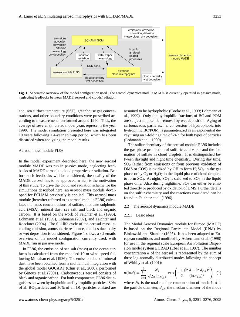
Fig. 1. Schematic overview of the model configuration used. The aerosol dynamics module MADE is currently operated in passive mode,neglecting feedbacks between MADE aerosol and clouds/radiation.
end, sea surface temperature (SST), greenhouse gas concen-trations, and other boundary conditions were prescribed ac-cording to measurements performed around 1990. Thus, theaverage of several simulated model years represents the year1990. The model simulation presented here was integrated10 years following a 4-year spin-up period, which has beendiscarded when analyzing the model results.
Aerosol mass module FL96
In the model experiment described here, the new aerosolmodule MADE was run in passive mode, neglecting feed-backs of MADE aerosol to cloud properties or radiation. Be-fore such feedbacks will be considered, the quality of theMADE aerosol has to be approved, which is the motivationof this study. To drive the cloud and radiation scheme for thesimulations described here, an aerosol mass module devel-oped for ECHAM previously is applied. This aerosol massmodule (hereafter referred to as aerosol module FL96) calcu-lates the mass concentrations of sulfate, methane sulphonicacid (MSA), mineral dust, sea salt, and black and organiccarbon. It is based on the work ofFeichter et al.(1996),Lohmann et al.(1999), Lohmann(2002), andFeichter andRoeckner(2004). The full life cycle of the aerosol mass in-cluding emission, atmospheric residence, and loss due to dryor wet deposition is considered. Figure1 shows a schematicoverview of the model configuration currently used, withMADE run in passive mode.
In FL96, the emission of sea salt (mass) at the ocean sur-faces is calculated from the modeled 10 m wind speed fol-lowing Monahan et al.(1986). The emission data of mineraldust have been obtained from a multiannual integration withthe global model GOCART (Chin et al., 2000), performedby Ginoux et al.(2001). Carbonaceous aerosol consists ofblack and organic carbon. For both components, FL96 distin-guishes between hydrophobic and hydrophilic particles. 80%of all BC-particles and 50% of all OC-particles emitted are
assumed to be hydrophobic (Cooke et al., 1999; Lohmann etal., 1999). Only the hydrophilic fractions of BC and POMare subject to potential removal by wet deposition. Aging ofcarbonaceous particles, i.e. conversion of hydrophobic intohydrophilic BC/POM, is parameterized as an exponential de-cay using an e-folding time of 24 h for both types of particles(Lohmann et al., 1999).
The sulfur chemistry of the aerosol module FL96 includesthe gas phase production of sulfuric acid vapor and the for-mation of sulfate in cloud droplets. It is distinguished be-tween daylight and night time chemistry. During day time,SO2 (either from emissions or from previous oxidation ofDMS or COS) is oxidized by OH to form H2SO4 in the gasphase or by O3 or H2O2 in the liquid phase of cloud dropletsto form SO4. At night, SO2 is oxidized to SO4 in the liquidphase only. Also during nighttime, SO2 can either be emit-ted directly or produced by oxidation of DMS. Further detailson the sulfur chemistry and the reactions considered can befound inFeichter et al.(1996).
2.2 The aerosol dynamics module MADE
2.2.1 Basic ideas
The Modal Aerosol Dynamics module for Europe (MADE)is based on the Regional Particulate Model (RPM) byBinkowski and Shankar(1995). It has been adapted to Eu-ropean conditions and modified byAckermann et al.(1998)for use in the regional scale European Air Pollution Disper-sion model system EURAD (Ebel et al., 1997). The numberconcentrationn of the aerosol is represented by the sum ofthree log-normally distributed modes following the conceptof Whitby et al.(1991):
n(ln d) =
3∑k=1
Nk√
2π ln σg,k
exp
(−
1
2
(ln d − ln dg,k)2
(ln σg,k)2
)(1)
whereNk is the total number concentration of modek, d isthe particle diameter,dg,k the median diameter of the mode
www.atmos-chem-phys.org/acp/5/3251/ Atmos. Chem. Phys., 5, 3251–3276, 2005
3254 A. Lauer et al.: Simulating aerosol microphysics with ECHAM/MADE
A. Lauer et al.: Simulating aerosol microphysics with ECHAM/MADE 23
ECHAM4/MADE
aerosol dynamicscondensation, nucleation,
coagulation,cloud-aerosol-interactions
tracer transportadvection,convection,
diffusion
removalsize dependent
wet & dry deposition,sedimentation
emissionsemissions of particles
and precursors
chemistrymultiphase sulfur chemistry,
gas-/particle equilibrium
Prozesse
particle diameter [µm]0.01 0.1 1.00.001 10.0 100.0
Aitken-mode
acc.mode
coarsemode
BC
SS
DUST
NH4+
SO42-
H2O
NO3-
EQSAM
OC
aerosol gas
clouds
NH3emissions(GEIA; 1990)
HNO3E4(DLR)/CHEM(climatology; 1990)
primary particleemissions
BC, OC, DUST, SS
SOA
SORGAM
organicprecursors
SO2
oxidation (gas)
H SO2 4
SO42-
H2O
emissions,oxidation ofDMS, COS
oxidation (cloud)
FL96
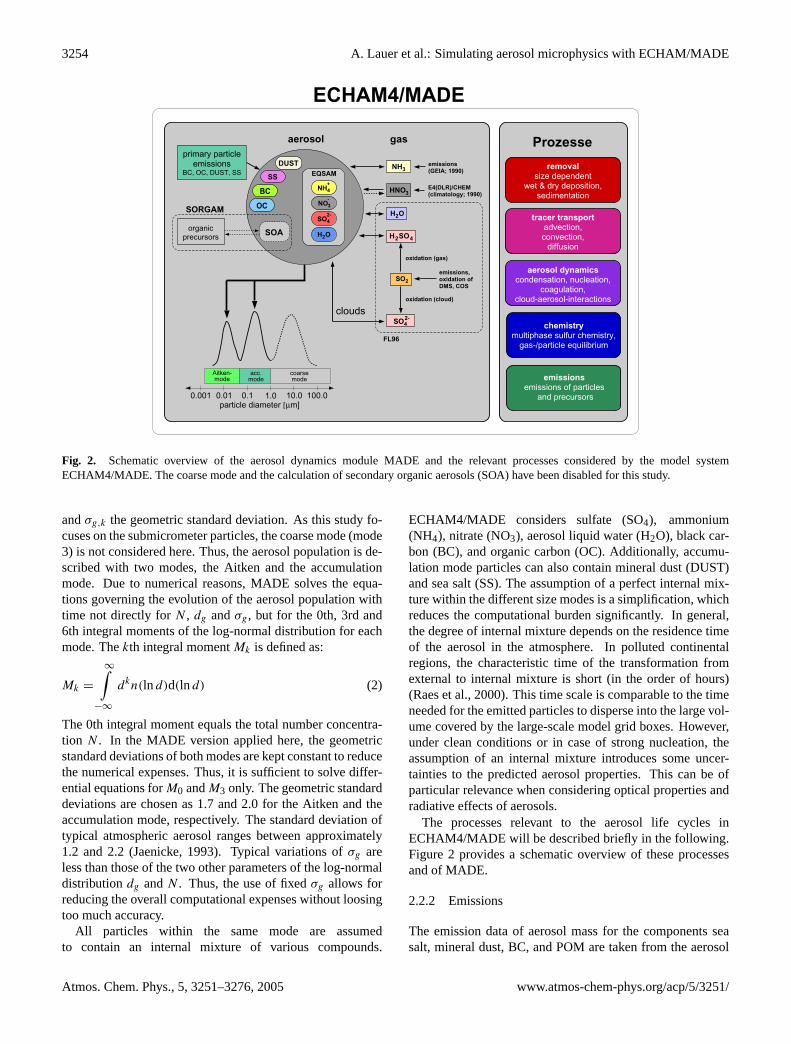
Fig. 2. Schematic overview of the aerosol dynamics moduleMADE and the relevant processes considered by the model sys-tem ECHAM4/MADE. The coarse mode and the calculation of sec-ondary organic aerosols (SOA) have been disabled for this study.
www.atmos-chem-phys.org/acp/0000/0001/ Atmos. Chem. Phys., 0000, 0001–36, 2005
Fig. 2. Schematic overview of the aerosol dynamics module MADE and the relevant processes considered by the model systemECHAM4/MADE. The coarse mode and the calculation of secondary organic aerosols (SOA) have been disabled for this study.
andσg,k the geometric standard deviation. As this study fo-cuses on the submicrometer particles, the coarse mode (mode3) is not considered here. Thus, the aerosol population is de-scribed with two modes, the Aitken and the accumulationmode. Due to numerical reasons, MADE solves the equa-tions governing the evolution of the aerosol population withtime not directly forN , dg andσg, but for the 0th, 3rd and6th integral moments of the log-normal distribution for eachmode. Thekth integral momentMk is defined as:
Mk =
∞∫−∞
dkn(ln d)d(ln d) (2)
The 0th integral moment equals the total number concentra-tion N . In the MADE version applied here, the geometricstandard deviations of both modes are kept constant to reducethe numerical expenses. Thus, it is sufficient to solve differ-ential equations forM0 andM3 only. The geometric standarddeviations are chosen as 1.7 and 2.0 for the Aitken and theaccumulation mode, respectively. The standard deviation oftypical atmospheric aerosol ranges between approximately1.2 and 2.2 (Jaenicke, 1993). Typical variations ofσg areless than those of the two other parameters of the log-normaldistributiondg andN . Thus, the use of fixedσg allows forreducing the overall computational expenses without loosingtoo much accuracy.
All particles within the same mode are assumedto contain an internal mixture of various compounds.
ECHAM4/MADE considers sulfate (SO4), ammonium(NH4), nitrate (NO3), aerosol liquid water (H2O), black car-bon (BC), and organic carbon (OC). Additionally, accumu-lation mode particles can also contain mineral dust (DUST)and sea salt (SS). The assumption of a perfect internal mix-ture within the different size modes is a simplification, whichreduces the computational burden significantly. In general,the degree of internal mixture depends on the residence timeof the aerosol in the atmosphere. In polluted continentalregions, the characteristic time of the transformation fromexternal to internal mixture is short (in the order of hours)(Raes et al., 2000). This time scale is comparable to the timeneeded for the emitted particles to disperse into the large vol-ume covered by the large-scale model grid boxes. However,under clean conditions or in case of strong nucleation, theassumption of an internal mixture introduces some uncer-tainties to the predicted aerosol properties. This can be ofparticular relevance when considering optical properties andradiative effects of aerosols.
The processes relevant to the aerosol life cycles inECHAM4/MADE will be described briefly in the following.Figure2 provides a schematic overview of these processesand of MADE.
2.2.2 Emissions
The emission data of aerosol mass for the components seasalt, mineral dust, BC, and POM are taken from the aerosol
Atmos. Chem. Phys., 5, 3251–3276, 2005 www.atmos-chem-phys.org/acp/5/3251/
A. Lauer et al.: Simulating aerosol microphysics with ECHAM/MADE 3255
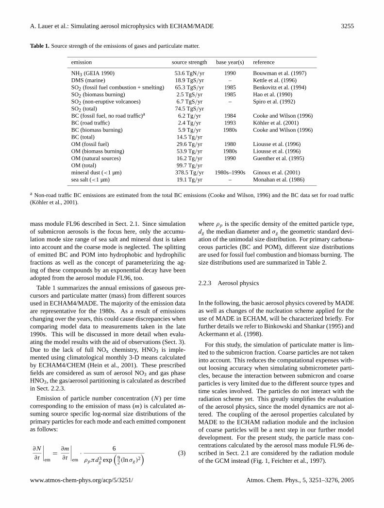
Table 1. Source strength of the emissions of gases and particulate matter.
emission source strength base year(s) reference
NH3 (GEIA 1990) 53.6 TgN/yr 1990 Bouwman et al.(1997)DMS (marine) 18.9 TgS/yr – Kettle et al.(1996)SO2 (fossil fuel combustion + smelting) 65.3 TgS/yr 1985 Benkovitz et al.(1994)SO2 (biomass burning) 2.5 TgS/yr 1985 Hao et al.(1990)SO2 (non-eruptive volcanoes) 6.7 TgS/yr – Spiro et al.(1992)SO2 (total) 74.5 TgS/yrBC (fossil fuel, no road traffic)a 6.2 Tg/yr 1984 Cooke and Wilson(1996)BC (road traffic) 2.4 Tg/yr 1993 Kohler et al.(2001)BC (biomass burning) 5.9 Tg/yr 1980s Cooke and Wilson(1996)BC (total) 14.5 Tg/yrOM (fossil fuel) 29.6 Tg/yr 1980 Liousse et al.(1996)OM (biomass burning) 53.9 Tg/yr 1980s Liousse et al.(1996)OM (natural sources) 16.2 Tg/yr 1990 Guenther et al.(1995)OM (total) 99.7 Tg/yrmineral dust (<1 µm) 378.5 Tg/yr 1980s–1990s Ginoux et al.(2001)sea salt (<1 µm) 19.1 Tg/yr – Monahan et al.(1986)
a Non-road traffic BC emissions are estimated from the total BC emissions (Cooke and Wilson, 1996) and the BC data set for road traffic(Kohler et al., 2001).
mass module FL96 described in Sect.2.1. Since simulationof submicron aerosols is the focus here, only the accumu-lation mode size range of sea salt and mineral dust is takeninto account and the coarse mode is neglected. The splittingof emitted BC and POM into hydrophobic and hydrophilicfractions as well as the concept of parameterizing the ag-ing of these compounds by an exponential decay have beenadopted from the aerosol module FL96, too.
Table1 summarizes the annual emissions of gaseous pre-cursors and particulate matter (mass) from different sourcesused in ECHAM4/MADE. The majority of the emission dataare representative for the 1980s. As a result of emissionschanging over the years, this could cause discrepancies whencomparing model data to measurements taken in the late1990s. This will be discussed in more detail when evalu-ating the model results with the aid of observations (Sect.3).Due to the lack of full NOx chemistry, HNO3 is imple-mented using climatological monthly 3-D means calculatedby ECHAM4/CHEM (Hein et al., 2001). These prescribedfields are considered as sum of aerosol NO3 and gas phaseHNO3, the gas/aerosol partitioning is calculated as describedin Sect.2.2.3.
Emission of particle number concentration (N) per timecorresponding to the emission of mass (m) is calculated as-suming source specific log-normal size distributions of theprimary particles for each mode and each emitted componentas follows:
∂N
∂t
∣∣∣∣em
=∂m
∂t
∣∣∣∣em
·6
ρpπd3g exp
(92(ln σg)2
) (3)
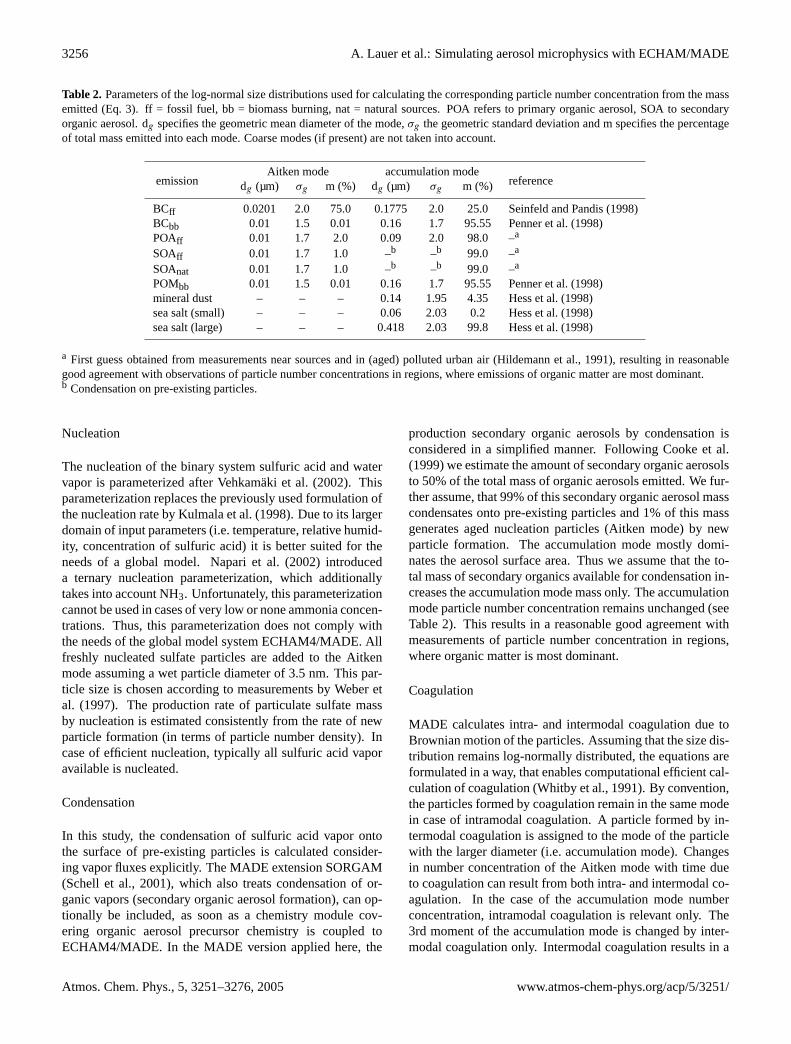
whereρp is the specific density of the emitted particle type,dg the median diameter andσg the geometric standard devi-ation of the unimodal size distribution. For primary carbona-ceous particles (BC and POM), different size distributionsare used for fossil fuel combustion and biomass burning. Thesize distributions used are summarized in Table2.
2.2.3 Aerosol physics
In the following, the basic aerosol physics covered by MADEas well as changes of the nucleation scheme applied for theuse of MADE in ECHAM, will be characterized briefly. Forfurther details we refer toBinkowski and Shankar(1995) andAckermann et al.(1998).
For this study, the simulation of particulate matter is lim-ited to the submicron fraction. Coarse particles are not takeninto account. This reduces the computational expenses with-out loosing accuracy when simulating submicrometer parti-cles, because the interaction between submicron and coarseparticles is very limited due to the different source types andtime scales involved. The particles do not interact with theradiation scheme yet. This greatly simplifies the evaluationof the aerosol physics, since the model dynamics are not al-tered. The coupling of the aerosol properties calculated byMADE to the ECHAM radiation module and the inclusionof coarse particles will be a next step in our further modeldevelopment. For the present study, the particle mass con-centrations calculated by the aerosol mass module FL96 de-scribed in Sect.2.1 are considered by the radiation moduleof the GCM instead (Fig.1, Feichter et al., 1997).
www.atmos-chem-phys.org/acp/5/3251/ Atmos. Chem. Phys., 5, 3251–3276, 2005
3256 A. Lauer et al.: Simulating aerosol microphysics with ECHAM/MADE
Table 2. Parameters of the log-normal size distributions used for calculating the corresponding particle number concentration from the massemitted (Eq.3). ff = fossil fuel, bb = biomass burning, nat = natural sources. POA refers to primary organic aerosol, SOA to secondaryorganic aerosol. dg specifies the geometric mean diameter of the mode,σg the geometric standard deviation and m specifies the percentageof total mass emitted into each mode. Coarse modes (if present) are not taken into account.
Aitken mode accumulation modeemission dg (µm) σg m (%) dg (µm) σg m (%) reference
BCff 0.0201 2.0 75.0 0.1775 2.0 25.0 Seinfeld and Pandis(1998)BCbb 0.01 1.5 0.01 0.16 1.7 95.55 Penner et al.(1998)POAff 0.01 1.7 2.0 0.09 2.0 98.0 –a
SOAff 0.01 1.7 1.0 –b –b 99.0 –a
SOAnat 0.01 1.7 1.0 –b –b 99.0 –a
POMbb 0.01 1.5 0.01 0.16 1.7 95.55 Penner et al.(1998)mineral dust – – – 0.14 1.95 4.35 Hess et al.(1998)sea salt (small) – – – 0.06 2.03 0.2 Hess et al.(1998)sea salt (large) – – – 0.418 2.03 99.8 Hess et al.(1998)
a First guess obtained from measurements near sources and in (aged) polluted urban air (Hildemann et al., 1991), resulting in reasonablegood agreement with observations of particle number concentrations in regions, where emissions of organic matter are most dominant.b Condensation on pre-existing particles.
Nucleation
The nucleation of the binary system sulfuric acid and watervapor is parameterized afterVehkamaki et al.(2002). Thisparameterization replaces the previously used formulation ofthe nucleation rate byKulmala et al.(1998). Due to its largerdomain of input parameters (i.e. temperature, relative humid-ity, concentration of sulfuric acid) it is better suited for theneeds of a global model.Napari et al.(2002) introduceda ternary nucleation parameterization, which additionallytakes into account NH3. Unfortunately, this parameterizationcannot be used in cases of very low or none ammonia concen-trations. Thus, this parameterization does not comply withthe needs of the global model system ECHAM4/MADE. Allfreshly nucleated sulfate particles are added to the Aitkenmode assuming a wet particle diameter of 3.5 nm. This par-ticle size is chosen according to measurements byWeber etal. (1997). The production rate of particulate sulfate massby nucleation is estimated consistently from the rate of newparticle formation (in terms of particle number density). Incase of efficient nucleation, typically all sulfuric acid vaporavailable is nucleated.
Condensation
In this study, the condensation of sulfuric acid vapor ontothe surface of pre-existing particles is calculated consider-ing vapor fluxes explicitly. The MADE extension SORGAM(Schell et al., 2001), which also treats condensation of or-ganic vapors (secondary organic aerosol formation), can op-tionally be included, as soon as a chemistry module cov-ering organic aerosol precursor chemistry is coupled toECHAM4/MADE. In the MADE version applied here, the
production secondary organic aerosols by condensation isconsidered in a simplified manner. FollowingCooke et al.(1999) we estimate the amount of secondary organic aerosolsto 50% of the total mass of organic aerosols emitted. We fur-ther assume, that 99% of this secondary organic aerosol masscondensates onto pre-existing particles and 1% of this massgenerates aged nucleation particles (Aitken mode) by newparticle formation. The accumulation mode mostly domi-nates the aerosol surface area. Thus we assume that the to-tal mass of secondary organics available for condensation in-creases the accumulation mode mass only. The accumulationmode particle number concentration remains unchanged (seeTable2). This results in a reasonable good agreement withmeasurements of particle number concentration in regions,where organic matter is most dominant.
Coagulation
MADE calculates intra- and intermodal coagulation due toBrownian motion of the particles. Assuming that the size dis-tribution remains log-normally distributed, the equations areformulated in a way, that enables computational efficient cal-culation of coagulation (Whitby et al., 1991). By convention,the particles formed by coagulation remain in the same modein case of intramodal coagulation. A particle formed by in-termodal coagulation is assigned to the mode of the particlewith the larger diameter (i.e. accumulation mode). Changesin number concentration of the Aitken mode with time dueto coagulation can result from both intra- and intermodal co-agulation. In the case of the accumulation mode numberconcentration, intramodal coagulation is relevant only. The3rd moment of the accumulation mode is changed by inter-modal coagulation only. Intermodal coagulation results in a
Atmos. Chem. Phys., 5, 3251–3276, 2005 www.atmos-chem-phys.org/acp/5/3251/
A. Lauer et al.: Simulating aerosol microphysics with ECHAM/MADE 3257
decrease of 3rd moment of the Aitken mode and an increaseof the 3rd moment of the accumulation mode.
Mode merging
The submicrometer aerosol in MADE is represented by thesum of two overlapping and interacting modes. This ap-proach allows a representation of the aerosol size distribu-tion typically found in measurements. Due to condensationor coagulation, the modes can grow with time and may be-come indistinguishable after a certain period of simulation,which is not being observed in nature. Hence, an algorithm isneeded, that handles the transfer of particles from the Aitkento the accumulation mode, i.e. allows particles to grow fromthe Aitken mode into the larger accumulation mode. This al-gorithm is called mode merging. To determine whether modemerging is necessary or not, the growth rates of both modesare compared to each other. The growth rates are given by theincreases in 3rd moment due to nucleation and condensationin the case of the Aitken mode and by condensation and in-termodal coagulation in the case of the accumulation mode.Once the growth rate of the Aitken mode exceeds that of theaccumulation mode, mode merging is being performed bycalculating the diameter of intersection between the Aitkenand accumulation mode number distributions and transfer-ring all Aitken mode particles larger than this diameter to theaccumulation mode (Binkowski et al., 1996). To ensure nu-merical stability, no more than one half of the Aitken modemass can be transferred to the accumulation mode within asingle time step.
2.2.4 Aerosol chemistry
The aerosol chemistry treats the chemical equilibrium sys-tem of sulfate, nitrate, ammonium, and water. The aerosolchemistry module originally implemented in MADE, basedon the equilibrium models MARS (Saxena et al., 1986) andSCAPE (Kim et al., 1993a,b), has been replaced by the Equi-librium Simplified Aerosol Model (EQSAM) v1.0 (Metzgeret al., 2002a,b). This reduces the overall computational ex-penses of ECHAM4/MADE significantly. The main purposeof EQSAM is to calculate the partitioning of NH3 and HNO3between gas phase and particles, as well as the aerosol liquidwater content. The aerosol liquid water content depends onthe chemical composition of the aerosol and the ambient rela-tive humidity. Aerosol water is treated just as all other chem-ical components. Thus an increase in aerosol water results inan increase of the total aerosol mass. With the particle num-ber concentration remaining constant in case of water up-take, the modal mean diameter of the corresponding aerosolmode increases. For more information on EQSAM includingtechnical details, further features, and a comparison with re-sults of conventional equilibrium models (e.g. ISORROPIA,Nenes et al., 1998), the reader is referred toMetzger et al.(2002a,b).
Sulfur chemistry
The sulfur chemistry implemented includes the productionof sulfuric acid vapor and sulfate dissolved in cloud droplets.This chemistry scheme has been adopted from the aerosolmass module FL96 (Sect.2.1) and was extended to explicitlytake into account NH4. The liquid phase reactions dependon how much SO2 can be dissolved in cloud droplets. Thesolubility of SO2 depends on the pH-value, which was es-timated byFeichter et al.(1996) assuming a molar ratio ofsulfate to ammonium of 1/1. This assumption is dispensablein ECHAM4/MADE as ammonia/ammonium is consideredexplicitly.
This could be achieved by extending the model to calcu-late the full life cycle of NH3. This includes emission fromvarious sources at the surface using the 1990 data set fromthe Global Emission Inventory Activity (GEIA) (Bouwmanet al., 1997) (Table1), consideration of dry and wet depo-sition of NH3 and the gas/aerosol partitioning between NH3and NH4.
2.2.5 Dry deposition
The basic concept of calculating the amount of particles re-moved by dry deposition per time step has been implementedin analogy to the aerosol mass module FL96 (Sect.2.1). Asa further development of FL96, the dry deposition velocitiesare not prescribed, but calculated for the 0th and 3rd momentof each mode from current meteorological conditions and theactual aerosol size distribution. The deposition velocityvd,k
of thekth moment is given by:
vd,k =1
ra + rb,k + rarb,kvs,k
+ vs,k (4)
(Slinn and Slinn, 1980), wherera is the aerodynamic resis-tance, rb,k the quasi-laminar layer resistance andvs,k thesedimentation velocity. The aerodynamic resistance is cal-culated followingGanzeveld and Lelieveld(1995) from theroughness lengthz0 and the boundary layer stability calcu-lated by ECHAM
ra =1
u∗κ
[ln
(z
z0
)− 8
( z
L
)](5)
whereu∗ is the friction velocity,κ the von-Karmann constant(=0.4), z the reference height (i.e. height of the middle ofthe lowest model layer),8 is a dimensionless stability term,andL the Monin-Obukhov-length. Following the concepts ofthe aerosol mass module FL96, the dry deposition of the gasphase species NH3, H2SO4, SO2, DMS is calculated usingprescribed dry deposition velocities (Table3).
2.2.6 Wet deposition and clouds
The removal of particulate matter and gaseous species is cal-culated from the GCM’s precipitation formation rate follow-ing the basic strategy used in the aerosol mass module FL96
www.atmos-chem-phys.org/acp/5/3251/ Atmos. Chem. Phys., 5, 3251–3276, 2005
3258 A. Lauer et al.: Simulating aerosol microphysics with ECHAM/MADE
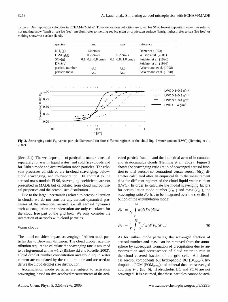
Table 3. Dry deposition velocities in ECHAM4/MADE. Three deposition velocities are given for SO2: lowest deposition velocities refer tonot melting snow (land) or sea ice (sea), medium refer to melting sea ice (sea) or dry/frozen surface (land), highest refer to sea (ice free) ormelting snow/wet surface (land).
species land sea reference
NH3(g) 1.0 cm/s – Dentener(1993)H2SO4(g) 0.2 cm/s 0.2 cm/s Wilson et al.(2001)SO2(g) 0.1; 0.2; 0.8 cm/s 0.1; 0.8; 1.0 cm/s Feichter et al.(1996)DMS(g) – – Feichter et al.(1996)particle number vd,0 vd,0 Ackermann et al.(1998)particle mass vd,3 vd,3 Ackermann et al.(1998)
0.00
0.25
0.50
0.75
1.00
Sca
veng
ing
Rat
io F
N
0.01 0.1 1d [µm]
LWC 0.1−0.2 g/m3
LWC 0.2−0.3 g/m3
LWC 0.3−0.4 g/m3
LWC > 0.4 g/m3
Fig. 3. Scavenging ratioFN versus particle diameter d for four different regimes of the cloud liquid water content (LWC) (Henning et al.,2002).
(Sect.2.1). The wet deposition of particulate matter is treatedseparately for warm (liquid water) and cold (ice) clouds andfor Aitken mode and accumulation mode particles. The rele-vant processes considered are in-cloud scavenging, below-cloud scavenging, and re-evaporation. In contrast to theaerosol mass module FL96, scavenging coefficients are notprescribed in MADE but calculated from cloud microphysi-cal properties and the aerosol size distribution.
Due to the large uncertainties related to aerosol alterationin clouds, we do not consider any aerosol dynamical pro-cesses of the interstitial aerosol, i.e. all aerosol dynamicssuch as coagulation or condensation are only calculated forthe cloud free part of the grid box. We only consider theinteraction of aerosols with cloud particles.
Warm clouds
The model considers impact scavenging of Aitken mode par-ticles due to Brownian diffusion. The cloud droplet size dis-tribution required to calculate the scavenging rate is assumedto be log-normal withσ=1.2 (Binkowski and Roselle, 2003).Cloud droplet number concentration and cloud liquid watercontent are calculated by the cloud module and are used toderive the cloud droplet size distribution.
Accumulation mode particles are subject to activationscavenging, based on size-resolved measurements of the acti-
vated particle fraction and the interstitial aerosol in cumulusand stratocumulus clouds (Henning et al., 2002). Figure3shows the scavenging ratio (ratio of scavenged aerosol frac-tion to total aerosol concentration) versus aerosol (dry) di-ameter calculated after an empirical fit to the measurementdata for different regimes of the cloud liquid water content(LWC). In order to calculate the modal scavenging factorsfor accumulation mode number (F0,l) and mass (F3,l), thescavenging ratioFN has to be integrated over the size distri-bution of the accumulation mode:
F0,l =1
N
∞∫0
n(d)FN (d)dd
F3,l =1
V
∞∫0
π
6d3n(d)FN (d)dd (6)
As for Aitken mode particles, the scavenged fraction ofaerosol number and mass can be removed from the atmo-sphere by subsequent formation of precipitation due to au-toconversion and accrenscence of cloud water to rain inthe cloud covered fraction of the grid cell. All chemi-cal aerosol components but hydrophobic BC (BCphob), hy-drophobic POM (POMphob) and mineral dust are scavengedapplyingF3,l (Eq. 6). Hydrophobic BC and POM are notscavenged. It is assumed, that these particles cannot be acti-
Atmos. Chem. Phys., 5, 3251–3276, 2005 www.atmos-chem-phys.org/acp/5/3251/
A. Lauer et al.: Simulating aerosol microphysics with ECHAM/MADE 3259
vated to cloud droplets. In analogy toLohmann(2002), weassume 90% of mineral dust to be hydrophobic and that theremaining 10% can be scavenged only. To take into accountthe hydrophobic mass fraction, the scavenging factor of ac-cumulation mode number concentrationF0,l is adjusted asfollows:
F ∗
0,l = F0,l ·
(1 −
M3(BCphob) + M3(POMphob) + 0.9 · M3(DUST)
M3(total)
)(7)
Finally, the number of activated aerosol particles is obtainedby multiplying the accumulation mode number concentrationby the scavenging ratioF ∗
0,l . The remaining interstitial par-ticles within the cloud are assumed to be unchanged by wetdeposition.
Cold clouds
The model takes into account activation scavenging of accu-mulation mode aerosol by ice clouds. Aitken mode particlesare not subject to activation scavenging, since such small par-ticles are poor freezing nuclei (e.g.Koop et al., 2000). Im-pact scavenging of aerosol by ice particles is neglected here,since this process is very inefficient due to the small numberconcentrations of ice crystals. The scavenging of accumu-lation mode mass by ice clouds is calculated in analogy toLohmann et al.(1999). Since the current knowledge on het-erogeneous ice nucleation is poor, we consider homogeneousnucleation as the major ice formation mechanism. Therefore,only hydrophilic particles are assumed to be scavenged. Incontrast toLohmann et al.(1999), a scavenging efficiencyof 5% is assumed instead of 10%, which improves the simu-lated mass concentrations in accordance to measurement datain the tropopause region (Hendricks et al., 2004). To esti-mate the corresponding scavenging of accumulation modenumber concentration from the scavenged mass fraction, it isassumed that only the largest particles of the log-normal sizedistribution are scavenged since the larger aerosol particlesare probably the most efficient freezing nuclei (e.g.Koop etal., 2000).
Below-cloud scavenging
Between cloud layers and below the lowest clouds, tracegases and hydrophilic particulate matter can be collected byfalling rain or snow and subsequently removed from the at-mosphere. The parameterization of below-cloud scavengingapplied here follows the approach ofBerge(1993).
Evaporation
Cloud droplets or ice crystals that have not been removedby precipitation evaporate once the cloud dissolves. Conse-quently, previously scavenged trace gases and aerosol par-ticles are released. It is assumed, that all of the releasedaerosols are in the size range of the accumulation mode,
as only accumulation mode particles are activated when thecloud forms and Aitken particles incorporated into clouds byimpact scavenging are released within cloud residues con-taining also accumulation mode particles. Thus, all Aitkenmode particles, which have undergone impact-scavengingand which have not been removed by precipitation, are as-sumed to become accumulation mode particles once thecloud evaporates. Hence Aitken mode mass is added tothe corresponding accumulation mode mass tracer. Parti-cle number concentration of scavenged Aitken mode parti-cles is not transfered to the accumulation mode and will bediscarded (Binkowski, 1999).
3 Comparison with observations
An evaluation of the results obtained from a first multian-nual integration with ECHAM4/MADE is required to eval-uate the ability of the new model system to reproduce ob-served aerosol distributions.
Principle difficulties arise when comparing GCM resultswith observations. First, due to the coarse spatial resolutionof the model, highly variable species such as particle num-ber concentration measured by individual ground based sta-tions can hardly be compared to simulated concentrations av-eraged over model grid cells representing a domain of thou-sands of square kilometers. The basic strategy followed hereto circumvent this problem is to average station data withina larger domain. Second, since ECHAM is designed as a cli-mate model (see Sects.2.1and2.2.2for details of the modelsetup and boundary conditions used), it is not capable to sim-ulate real episodes. Thus, measurements taken at a specificperiod of time cannot be compared to the model results di-rectly, but based on climatological means only. Therefore,only long-term data covering several weeks or months areapplied here for intercomparison with model data.
3.1 Global aerosol distribution
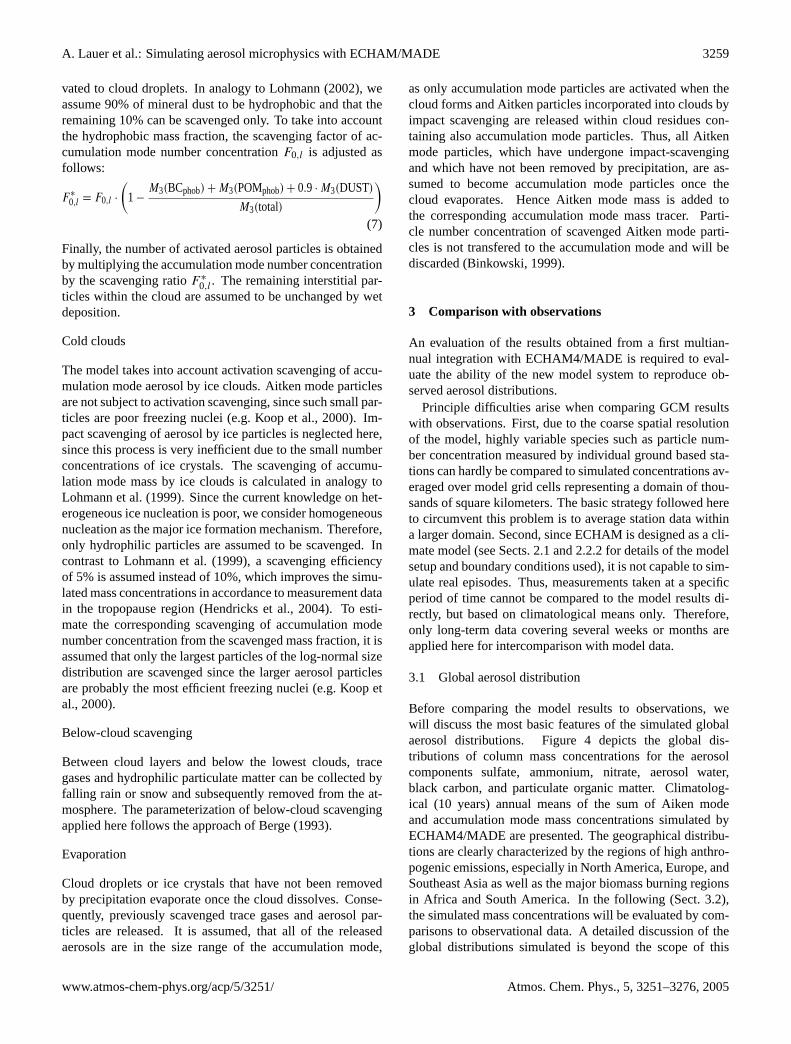
Before comparing the model results to observations, wewill discuss the most basic features of the simulated globalaerosol distributions. Figure4 depicts the global dis-tributions of column mass concentrations for the aerosolcomponents sulfate, ammonium, nitrate, aerosol water,black carbon, and particulate organic matter. Climatolog-ical (10 years) annual means of the sum of Aiken modeand accumulation mode mass concentrations simulated byECHAM4/MADE are presented. The geographical distribu-tions are clearly characterized by the regions of high anthro-pogenic emissions, especially in North America, Europe, andSoutheast Asia as well as the major biomass burning regionsin Africa and South America. In the following (Sect.3.2),the simulated mass concentrations will be evaluated by com-parisons to observational data. A detailed discussion of theglobal distributions simulated is beyond the scope of this
www.atmos-chem-phys.org/acp/5/3251/ Atmos. Chem. Phys., 5, 3251–3276, 2005
3260 A. Lauer et al.: Simulating aerosol microphysics with ECHAM/MADE
sulfate (SO4) ammonium (NH4)
nitrate (NO3) aerosol water (H2O)
black carbon (BC) particulate organic matter (POM)
0 0.005 0.01 0.025 0.05 0.1 0.25 0.5 1 2.5 5 10 25 50 100[mg/m2]
Fig. 4. Climatological annual means of the column mass concentrations (mg/m2) of the aerosol components SO4, NH4, NO3, H2O, BC, andPOM in fine particles (sum of Aitken and accumulation mode) obtained from a 10-year integration with the model system ECHAM4/MADE.
paper since it is intended to focus on the description andevaluation of the new model system. A detailed analysis ofthe properties of the global submicrometer aerosol simulatedwith ECHAM4/MADE, an interpretation of the results, andan examination of the role of aerosol dynamics on the globalscale will be provided by a separate paper (Part II: Resultsfrom a first multiannual integration).
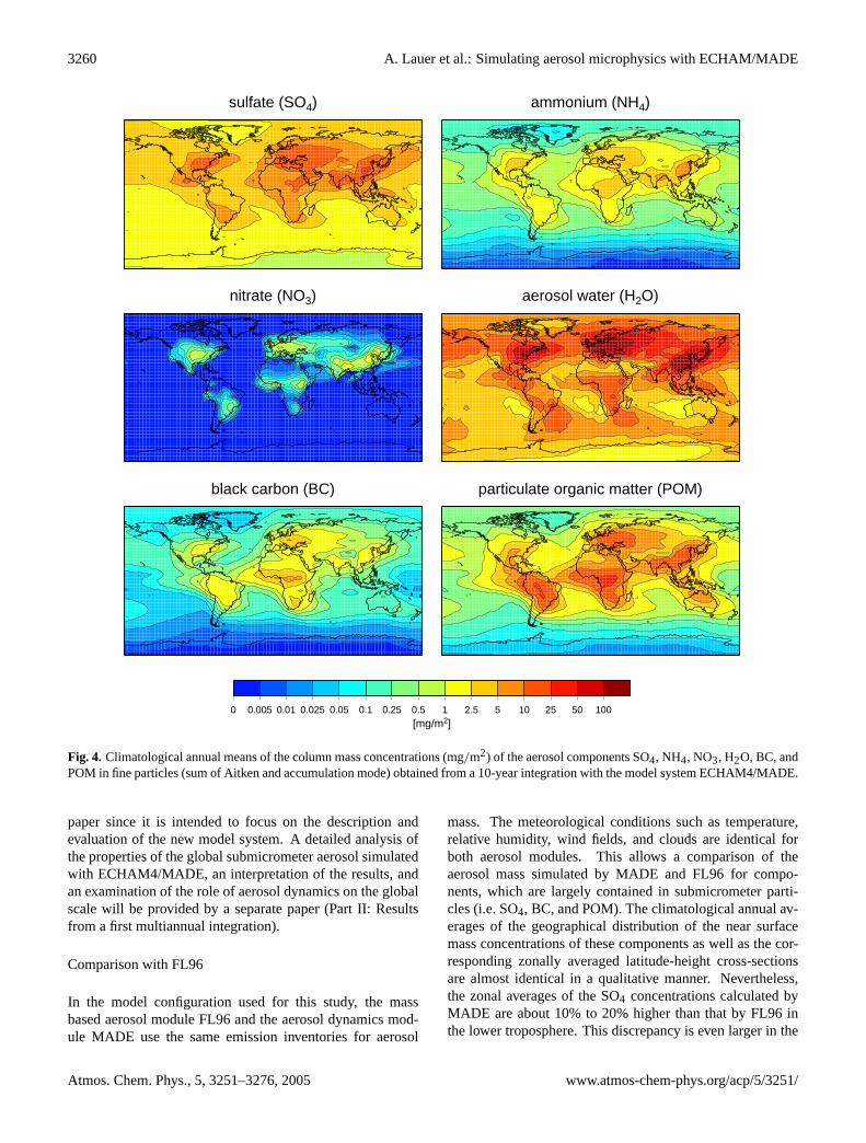
Comparison with FL96
In the model configuration used for this study, the massbased aerosol module FL96 and the aerosol dynamics mod-ule MADE use the same emission inventories for aerosol
mass. The meteorological conditions such as temperature,relative humidity, wind fields, and clouds are identical forboth aerosol modules. This allows a comparison of theaerosol mass simulated by MADE and FL96 for compo-nents, which are largely contained in submicrometer parti-cles (i.e. SO4, BC, and POM). The climatological annual av-erages of the geographical distribution of the near surfacemass concentrations of these components as well as the cor-responding zonally averaged latitude-height cross-sectionsare almost identical in a qualitative manner. Nevertheless,the zonal averages of the SO4 concentrations calculated byMADE are about 10% to 20% higher than that by FL96 inthe lower troposphere. This discrepancy is even larger in the
Atmos. Chem. Phys., 5, 3251–3276, 2005 www.atmos-chem-phys.org/acp/5/3251/

A. Lauer et al.: Simulating aerosol microphysics with ECHAM/MADE 3261
0.0
1.2
2.4
3.6
4.8
6.0
7.2
8.4
9.6
part
icle
mas
s [µ
g/m
3 ]
Jan Feb Mar Apr May Jun Jul Aug Sep Oct Nov Dec
ECHAM4/MADE SO4
ECHAM4/MADE NO3
ECHAM4/MADE BCECHAM4/MADE OCIMPROVE SO4 (1995-2000)IMPROVE NO3 (1995-2000)IMPROVE BC (1995-2000)IMPROVE OC (1995-2000)
Fig. 5. Climatological seasonal cycle of observed and modeled near surface mass concentrations of the aerosol components SO4, NO3,BC, and OC in fine particles (PM2.5), averaged over the south-eastern part of the USA. The error bars denote the standard deviation of theindividual monthly means to the climatological average.
upper troposphere. Nevertheless, the mass concentrations ofSO4 in the upper troposphere calculated by both modules areabout two orders of magnitude smaller than that in the lowertroposphere. In case of POM, the mass concentrations cal-culated by MADE are about 20% higher than that of FL96in the regions with significant POM mass concentrations(about 50◦ S–60◦ N). In contrast to SO4, these differencesdo not vary much with height. For BC, the differences be-tween FL96 and MADE are less distinctive. Whereas MADEshows lower BC concentrations in the northern hemisphere(up to about 20%), MADE shows higher BC concentra-tions in the southern hemisphere (about 10%). Nevertheless,the total burdens of these aerosol components simulated byboth modules are quite similar. For SO4, MADE calculates2.25 Tg versus 2.18 Tg (FL96), for BC 0.26 Tg (MADE) ver-sus 0.23 Tg (FL96), and for POM 1.77 Tg (MADE) versus1.46 Tg (FL96).
Thus, the calculation of aerosol dynamical processesseems to be less essential for the simulation of the totalaerosol mass than for the simulation of particle number con-centration and size-distribution. This will be discussed bythe separate paper mentioned above in more detail.
3.2 Near surface mass concentrations
3.2.1 United States
To evaluate the modeled near surface mass concentrations,we use observational data taken within the InteragencyMonitoring of Protected Visual Environments (IMPROVE),which is a cooperative monitoring program of the UnitedStates Environmental Protection Agency (EPA), federal landmanagement agencies, and state air agencies (Malm et al.,2000). Besides other tasks, aerosols (mass) and visibilityare measured on a regularly basis by many stations, locatedin national parks, national wildlife refuges, and other pro-tected areas all over the United States. Measurement dataof several years are available (IMPROVE:http://vista.cira.colostate.edu/improve/).
An intercomparison of IMPROVE data withECHAM4/MADE is performed based on climatologi-cal monthly means. The model data are averaged over all10 model years. The IMPROVE data shown here representaverages of the years 1995 to 2000. In order to avoid anyimproper weighting of areas with different densities ofmeasurement sites, all data from sites located within thesame ECHAM T30 grid cell are averaged before any furtherprocessing. The measurements were taken near the surface.Thus, the model results calculated for the lowest modellayer are used for the intercomparison. In order to obtaina quantitative measure for the differences between modeland observations, the normalized mean error (NME) iscalculated as follows:
NME =
∑Ni=1 |modeli − observationi |∑N
i=1 observationi· 100% (8)
In case of the seasonal cycles, modeli is the climatologicalmodel data for month i, observationi the corresponding mea-surement data and N is the number of months (=12). Whencalculating the normalized mean error of the geographicaldistribution, i loops over all T30 grid cells with observationaldata available and N is the total number of grid cells withmeasurement data.
Seasonal cycle
Figure5 shows the seasonal cycle of aerosol components infine particles (PM2.5, i.e. d<2.5 µm), measured by the IM-PROVE network and calculated by ECHAM4/MADE. Themass concentrations of the aerosol components compared aredominated by fine particles in the size-range of the Aitkenand the accumulation mode, which allows a comparison ofthe measured PM2.5 concentrations with the model, whichcurrently neglects a coarse mode. All available values havebeen averaged over the south-eastern part of the USA (≈77◦–96◦ W, 30◦–41◦ N). This region of North America is charac-terized by high anthropogenic emissions of SO2, BC, andOC.
www.atmos-chem-phys.org/acp/5/3251/ Atmos. Chem. Phys., 5, 3251–3276, 2005

3262 A. Lauer et al.: Simulating aerosol microphysics with ECHAM/MADE
Both, model and observations show maximum sulfate con-centrations in summer and minimum concentrations in win-ter. There is no systematic under- or overestimation by themodel. The averaged normalized mean error of the modeledsulfate is 10%. The seasonal cycle of nitrate is in oppositephase with sulfate, showing a maximum in winter and a min-imum in summer. ECHAM4/MADE reproduces the sum-mer minimum only. The winter maximum of the observedvalues is not shown by the model. The NME for nitrate is39%. During most of the year, NO3 is underestimated bythe model with respect to the measurements. This discrep-ancy in the seasonal cycle of NO3 could be related to theuse of a HNO3 climatology, which cannot respond to cur-rent meteorological conditions. Both the model and observedBC concentrations show almost no seasonal cycle. However,ECHAM4/MADE shows much higher BC concentrationsthan the IMPROVE measurements. On average, the modelresults are 2–3 times higher than the corresponding observa-tions. The NME amounts to 143%. This large overestimationby the model can be, at least partially, explained by the loca-tions of the measurement sites. While all IMPROVE stationsare located in remote areas such as national parks or wildliferefuges, the large ECHAM T30 grid cells also contain theemissions of the urban areas and different kinds of traffic.Particulate SO4 and NO3 are secondary aerosols. The timeneeded to transform precursors such as SO2 or NOx from gasto particle phase allows transport away from the sources, re-sulting in a geographical distribution following the patternof the emissions less distinctive than primary particles suchas BC. Thus, it can be assumed, that the background val-ues of the IMPROVE network are more representative forthe secondary aerosols than for the primary BC when con-sidering the large domains covered by a ECHAM T30 gridcell. Another important reason for the overestimation of BCby the model might be the emission data used. Currently,global BC-emissions byCooke and Wilson(1996), represen-tative for the year 1984, are used. The corresponding emis-sion rates are about 40% higher compared to the more recentemission data set byBond et al.(2004), which represent theyear 1996. Similar to BC, OC shows no distinct seasonalcycle in the observations. On average, the normalized meanerror of OC is 38%. The modeled OC mass concentrationsare systematically higher than the observations. As in thecase of BC, the more recent emission data for OC fromBondet al.(2004) show a lower annual source strength than the OCemission data currently used. Thus, lower OC concentrationsare to be expected when updating the emission data.
Geographical distribution
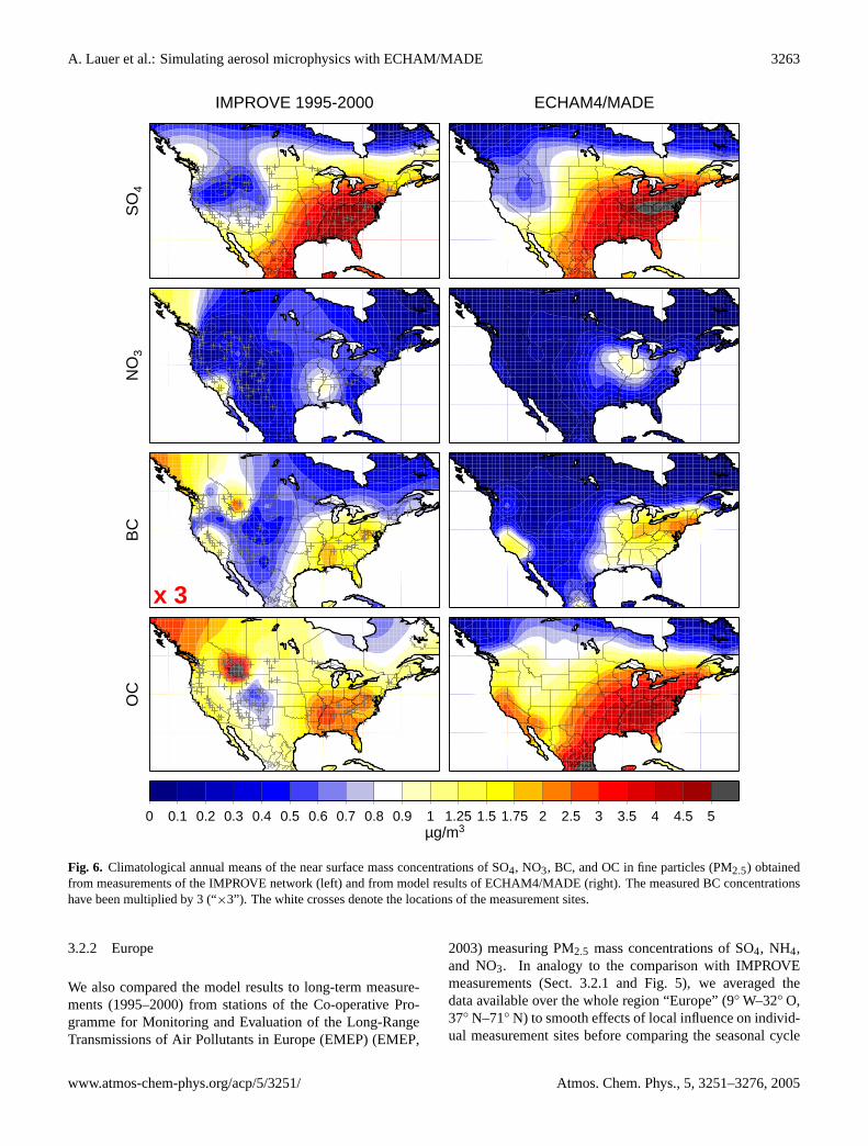
The annual mean geographical distributions of the aerosolcomponents SO4, NO3, BC, and OC derived from the IM-PROVE measurements and the model simulation are de-picted by Fig.6. Care has to be taken when interpretingregions with no measurement sites. These gaps have been
filled by the gridding and interpolation algorithms of the plotsoftware. Thus, the figure includes white crosses to mark themeasurement sites with observational data available.
Both model and observations show a distinctive west-eastgradient in the geographical distributions of the SO4 masswith high concentrations found in the eastern part of theUnited States and low values in the western part. A minordifference between model and observations is the deviationin the exact location of the region with maximum sulfate con-centrations in the eastern United States. According to themeasurements, the maximum is located about 500–800 kmfarther north-easterly in the model. However, running at T30resolution (Sect.2.1), this distance equals 1–2 model gridcells only. The normalized mean error for sulfate is 25%.
The maximum nitrate concentrations shown by the modelas well as by the observations are about 1 µg/m3. Similar tosulfate, the region of maximum nitrate in the eastern UnitedStates is shifted in the model 1–2 T30 grid cells farther north-easterly. A second maximum located in the Los Angles basinof California is not reproduced by ECHAM4/MADE. Over-all, nitrate concentrations are underestimated by the modelwith respect to the measurements (NME for NO3 is 66%).
Since a direct intercomparison of the geographical distri-bution of BC is difficult due to the lower values observed,the measurement data have been multiplied by a factor of3 (marked as “×3” in Fig. 6) to allow for a better compar-ison of the geographical patterns with the model data (see“seasonal cycle” in the previous section). Similar to NO3,BC shows increased concentrations within a region of theeastern United States and within a second region of smallerextent in California. These patterns are reproduced by themodel. In addition, the observed geographical BC distribu-tion shows an isolated maximum over Montana, which is notreproduced by the model. This maximum is a result of asingle heavy forest fire event in summer 2000. Such singleevents cannot be reproduced by the model running in quasi-equilibrium mode using the same emission data every year.As already obvious from the comparison of the seasonal cy-cles, BC is overestimated by the model, resulting in a NMEof 135% (see “seasonal cycle” in the previous section).
The patterns of the geographical OC distributions mostlyfollow those of the BC distribution. The maximum OC con-centrations measured and calculated by the model are bothabout 3 µg/m3, but the modeled areas of high OC concen-trations have a larger extent than shown by the observations.As in the BC data, also OC observations show an isolatedmaximum over Montana, which is likely produced by theheavy forest fires in summer 2000. In contrast, the modelwhich does not include such single events in the emissiondata, shows minimum OC concentrations in this region. Withregard to the overall representation of BC and OC by themodel, the comparison shows that the agreement betweenmodel and measurements is much better for OC than for BC.The NME amounts to 47% in the case of OC.
Atmos. Chem. Phys., 5, 3251–3276, 2005 www.atmos-chem-phys.org/acp/5/3251/
A. Lauer et al.: Simulating aerosol microphysics with ECHAM/MADE 3263
IMPROVE 1995-2000
SO
4
ECHAM4/MADE
NO
3B
C
x 3
OC
0 0.1 0.2 0.3 0.4 0.5 0.6 0.7 0.8 0.9 1 1.25 1.5 1.75 2 2.5 3 3.5 4 4.5 5µg/m3
Fig. 6. Climatological annual means of the near surface mass concentrations of SO4, NO3, BC, and OC in fine particles (PM2.5) obtainedfrom measurements of the IMPROVE network (left) and from model results of ECHAM4/MADE (right). The measured BC concentrationshave been multiplied by 3 (“×3”). The white crosses denote the locations of the measurement sites.
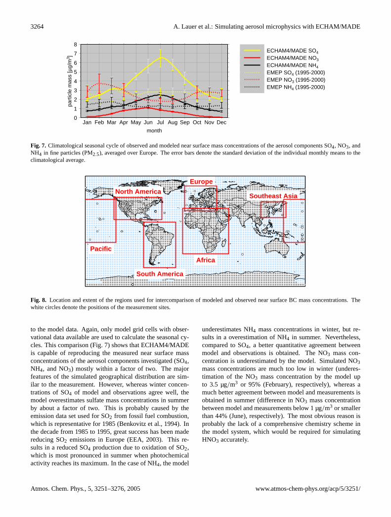
3.2.2 Europe
We also compared the model results to long-term measure-ments (1995–2000) from stations of the Co-operative Pro-gramme for Monitoring and Evaluation of the Long-RangeTransmissions of Air Pollutants in Europe (EMEP) (EMEP,
2003) measuring PM2.5 mass concentrations of SO4, NH4,and NO3. In analogy to the comparison with IMPROVEmeasurements (Sect.3.2.1 and Fig. 5), we averaged thedata available over the whole region “Europe” (9◦ W–32◦ O,37◦ N–71◦ N) to smooth effects of local influence on individ-ual measurement sites before comparing the seasonal cycle
www.atmos-chem-phys.org/acp/5/3251/ Atmos. Chem. Phys., 5, 3251–3276, 2005
3264 A. Lauer et al.: Simulating aerosol microphysics with ECHAM/MADE
0
1
2
3
4
5
6
7
8
part
icle
mas
s [µ
g/m
3 ]
month
Jan Feb Mar Apr May Jun Jul Aug Sep Oct Nov Dec
ECHAM4/MADE SO4
ECHAM4/MADE NO3
ECHAM4/MADE NH4
EMEP SO4 (1995-2000)EMEP NO3 (1995-2000)EMEP NH4 (1995-2000)
Fig. 7. Climatological seasonal cycle of observed and modeled near surface mass concentrations of the aerosol components SO4, NO3, andNH4 in fine particles (PM2.5), averaged over Europe. The error bars denote the standard deviation of the individual monthly means to theclimatological average.
Europe
Africa
North America
South America
Southeast Asia
Pacific
Fig. 8. Location and extent of the regions used for intercomparison of modeled and observed near surface BC mass concentrations. Thewhite circles denote the positions of the measurement sites.
to the model data. Again, only model grid cells with obser-vational data available are used to calculate the seasonal cy-cles. This comparison (Fig.7) shows that ECHAM4/MADEis capable of reproducing the measured near surface massconcentrations of the aerosol components investigated (SO4,NH4, and NO3) mostly within a factor of two. The majorfeatures of the simulated geographical distribution are sim-ilar to the measurement. However, whereas winter concen-trations of SO4 of model and observations agree well, themodel overestimates sulfate mass concentrations in summerby about a factor of two. This is probably caused by theemission data set used for SO2 from fossil fuel combustion,which is representative for 1985 (Benkovitz et al., 1994). Inthe decade from 1985 to 1995, great success has been madereducing SO2 emissions in Europe (EEA, 2003). This re-sults in a reduced SO4 production due to oxidation of SO2,which is most pronounced in summer when photochemicalactivity reaches its maximum. In the case of NH4, the model
underestimates NH4 mass concentrations in winter, but re-sults in a overestimation of NH4 in summer. Nevertheless,compared to SO4, a better quantitative agreement betweenmodel and observations is obtained. The NO3 mass con-centration is underestimated by the model. Simulated NO3mass concentrations are much too low in winter (underes-timation of the NO3 mass concentration by the model upto 3.5 µg/m3 or 95% (February), respectively), whereas amuch better agreement between model and measurements isobtained in summer (difference in NO3 mass concentrationbetween model and measurements below 1 µg/m3 or smallerthan 44% (June), respectively). The most obvious reason isprobably the lack of a comprehensive chemistry scheme inthe model system, which would be required for simulatingHNO3 accurately.
Atmos. Chem. Phys., 5, 3251–3276, 2005 www.atmos-chem-phys.org/acp/5/3251/
A. Lauer et al.: Simulating aerosol microphysics with ECHAM/MADE 3265
North America
1
10
100
1000
10000
EC
HA
M4/
MA
DE
[ng/
m3 ]
1 10 100 1000 10000surface measurements [ng/m3]
Europe
1
10
100
1000
10000
EC
HA
M4/
MA
DE
[ng/
m3 ]
1 10 100 1000 10000surface measurements [ng/m3]
Southeast Asia
1
10
100
1000
10000
EC
HA
M4/
MA
DE
[ng/
m3 ]
1 10 100 1000 10000surface measurements [ng/m3]
South America
1
10
100
1000
10000
EC
HA
M4/
MA
DE
[ng/
m3 ]
1 10 100 1000 10000surface measurements [ng/m3]
Africa
1
10
100
1000
10000
EC
HA
M4/
MA
DE
[ng/
m3 ]
1 10 100 1000 10000surface measurements [ng/m3]
Pacific Ocean
1
10
100
1000
10000
EC
HA
M4/
MA
DE
[ng/
m3 ]
1 10 100 1000 10000surface measurements [ng/m3]
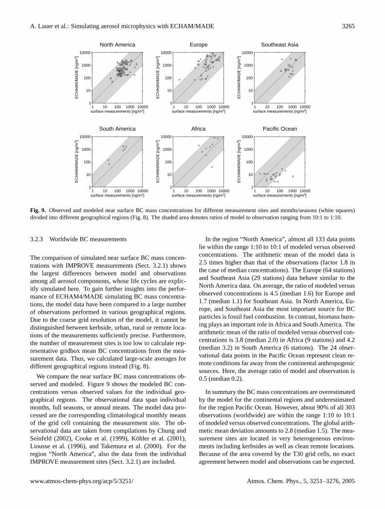
Fig. 9. Observed and modeled near surface BC mass concentrations for different measurement sites and months/seasons (white squares)divided into different geographical regions (Fig.8). The shaded area denotes ratios of model to observation ranging from 10:1 to 1:10.
3.2.3 Worldwide BC measurements
The comparison of simulated near surface BC mass concen-trations with IMPROVE measurements (Sect.3.2.1) showsthe largest differences between model and observationsamong all aerosol components, whose life cycles are explic-itly simulated here. To gain further insights into the perfor-mance of ECHAM4/MADE simulating BC mass concentra-tions, the model data have been compared to a large numberof observations performed in various geographical regions.Due to the coarse grid resolution of the model, it cannot bedistinguished between kerbside, urban, rural or remote loca-tions of the measurements sufficiently precise. Furthermore,the number of measurement sites is too low to calculate rep-resentative gridbox mean BC concentrations from the mea-surement data. Thus, we calculated large-scale averages fordifferent geographical regions instead (Fig.8).
We compare the near surface BC mass concentrations ob-served and modeled. Figure9 shows the modeled BC con-centrations versus observed values for the individual geo-graphical regions. The observational data span individualmonths, full seasons, or annual means. The model data pro-cessed are the corresponding climatological monthly meansof the grid cell containing the measurement site. The ob-servational data are taken from compilations byChung andSeinfeld(2002), Cooke et al.(1999), Kohler et al.(2001),Liousse et al.(1996), andTakemura et al.(2000). For theregion “North America”, also the data from the individualIMPROVE measurement sites (Sect.3.2.1) are included.
In the region “North America”, almost all 133 data pointslie within the range 1:10 to 10:1 of modeled versus observedconcentrations. The arithmetic mean of the model data is2.5 times higher than that of the observations (factor 1.8 inthe case of median concentrations). The Europe (64 stations)and Southeast Asia (29 stations) data behave similar to theNorth America data. On average, the ratio of modeled versusobserved concentrations is 4.5 (median 1.6) for Europe and1.7 (median 1.1) for Southeast Asia. In North America, Eu-rope, and Southeast Asia the most important source for BCparticles is fossil fuel combustion. In contrast, biomass burn-ing plays an important role in Africa and South America. Thearithmetic mean of the ratio of modeled versus observed con-centrations is 3.8 (median 2.0) in Africa (9 stations) and 4.2(median 3.2) in South America (6 stations). The 24 obser-vational data points in the Pacific Ocean represent clean re-mote conditions far away from the continental anthropogenicsources. Here, the average ratio of model and observation is0.5 (median 0.2).
In summary the BC mass concentrations are overestimatedby the model for the continental regions and underestimatedfor the region Pacific Ocean. However, about 90% of all 303observations (worldwide) are within the range 1:10 to 10:1of modeled versus observed concentrations. The global arith-metic mean deviation amounts to 2.8 (median 1.5). The mea-surement sites are located in very heterogeneous environ-ments including kerbsides as well as clean remote locations.Because of the area covered by the T30 grid cells, no exactagreement between model and observations can be expected.
www.atmos-chem-phys.org/acp/5/3251/ Atmos. Chem. Phys., 5, 3251–3276, 2005

3266 A. Lauer et al.: Simulating aerosol microphysics with ECHAM/MADE
200
300
400
500
600
700
800
900
1000
pres
sure
[hP
a]
10 100 1000 10000concentration [cm-3]
N5 (d > 5 nm)200
300
400
500
600
700
800
900
1000
pres
sure
[hP
a]
10 100 1000 10000concentration [cm-3]
N15 (d > 15 nm)200
300
400
500
600
700
800
900
1000
pres
sure
[hP
a]
1 10 100 1000concentration [cm-3]
N120 (d > 120 nm)
ECHAM4/MADE median
ECHAM4/MADE 25%, 75% percentiles
LACE median
LACE 25%, 75% percentiles
Fig. 10. Vertical profiles of aerosol number concentration (ambient, not STP conditions as in Fig.11) in north-east Germany obtained frommeasurements during LACE (Petzold et al., 2002) (dashed) and calculated by ECHAM4/MADE (solid) for the 3 size classes of particleslarger than 5 nm, 15 nm, and 120 nm.
However, this comparison shows, that ECHAM4/MADE iscapable to reproduce the range of observations of BC massconcentrations found in polluted areas as well as in clean re-mote areas, which spans almost three orders of magnitude.The major geographical differences are captured correctly bythe model.
3.2.4 Particle mass concentration – conclusions
The comparisons of measured and modeled aerosol massconcentrations show that ECHAM4/MADE is capable to re-produce the observed seasonal cycle and major features ofthe geographical distribution reasonably well. Quantitativedifferences are mostly within a factor of two with the excep-tion of BC and NO3. In view of the basic difficulties anduncertainties when comparing climatological coarse resolu-tion model output with measurements, this is a notable result.However, the comparison also shows that an updated emis-sion data set should be adopted to reduce some of the differ-ences found, in particular for BC particles. To reduce the un-certainties in particulate NO3, a comprehensive atmosphericchemistry scheme should be coupled to ECHAM4/MADE.
3.3 Number concentration
3.3.1 Central Europe
During the Lindenberg Aerosol Characterization Experiment(LACE) performed in the summer of 1998, optical and mi-crophysical aerosol properties were measured over north-eastern Germany (≈13.5◦–14.5◦ E, 51.5◦–52.7◦ N) from twoaircraft. Ten flights have been accomplished between 31 July
and 12 August covering the vertical range from minimumflight altitude (150 m above ground) to tropopause height.The measurement site can be regarded as typical of pol-luted continental summer conditions in Central Europe. Thedata set used for intercomparison with ECHAM4/MADEcontains the ambient (i.e. not converted to STP conditions)median particle number concentrations of particles in threedifferent size ranges (dry diameters d>5 nm, 15 nm, and120 nm, hereafter referred to as N5, N15, and N120, re-spectively) (Petzold et al., 2002). Particles with d>120 nmroughly meet the accumulation mode, N15 is dominated byAitken mode particles and N5 includes fresh ultrafine nucleiadditionally. Figure10 presents a comparison of model datawith these measurements. The variability is given by the cor-responding 25%- and 75%-percentiles. The measurementswere taken under cloud free conditions. Thus, model datawith a cloud fraction of the corresponding grid cell above10% were not taken into account. Model data from Augustof each year simulated were used. The percentiles shown inFig. 10 for the model data were calculated from 12 h meansof the modeled number concentration.
The median of the modeled particle number concentra-tion N5 stays within the measured variability in the altituderange from the surface up to pressure levels between 700and 650 hPa. In the boundary layer up to about 900 hPa,the modeled variability is much less than observed. Thisindicates, that the near surface particle number concentra-tions are clearly dominated by the emissions of primary par-ticles, which remain constant during the respective month. Inthe free troposphere and above, N5 is systematically smallercompared to the observations. Nevertheless, the modeled
Atmos. Chem. Phys., 5, 3251–3276, 2005 www.atmos-chem-phys.org/acp/5/3251/
A. Lauer et al.: Simulating aerosol microphysics with ECHAM/MADE 3267
200
300
400
500
600
700
800
900
1000
pres
sure
[hP
a]
100 1000 10000concentration [cm-3 STP]
70˚S-20˚S
200
300
400
500
600
700
800
900
1000
pres
sure
[hP
a]
100 1000 10000concentration [cm-3 STP]
20˚S-20˚N
200
300
400
500
600
700
800
900
1000
pres
sure
[hP
a]
100 1000 10000concentration [cm-3 STP]
20˚N-70˚N
ECHAM4/MADE (≥ 0.003 µm)
Clarke UCN (0.003 - 3.0 µm)
Fig. 11. Vertical profiles of mean aerosol number concentrations (STP conditions: 273 K, 1013 hPa) obtained from various measurementcampaigns over the Pacific Ocean (Clarke and Kapustin, 2002) (dashed) and ECHAM4/MADE (solid) for the 3 latitude bands 70◦ S–20◦ S,20◦ S–20◦ N, and 20◦ N–70◦ N. The error bars depict the standard deviation (positive part shown only).
variability increases with altitude and the median of the ob-served number concentrations stays within the modeled vari-ability below the 400 to 350 hPa pressure levels. The in-creased variability is a result of enhanced particle formationby nucleation, which is most effective in the upper tropo-sphere.
The vertical profile of N15 is similar to that of N5 in aqualitative manner. Good agreement between model and ob-servation is found in the lower and middle troposphere belowthe 600 hPa pressure level. Above this altitude range, mod-eled number concentrations are systematically lower than ob-served. In contrast to N5, the modeled variability decreasesin the upper troposphere. This indicates, that the modeledaerosol within this size range is hardly influenced by forma-tion of new particles by nucleation.
N120 is about one order of magnitude lower than N5. Up to350 hPa, the modeled median stays within the variability ofthe measurements. The peak in observed number concentra-tion at about 500 hPa is related to intercontinental long-rangetransport of particles from boreal forest fires in North Amer-ica (Petzold et al., 2002). Thus, the elevated number con-centrations in this altitude range do not reflect backgroundconditions. Above 350 hPa, modeled particle number con-centrations as well as corresponding variabilities are system-atically smaller than shown by the observations.
The general underestimation of the particle number con-centration in the upper troposphere could be a direct resultof the prediction of smaller average particle diameters thanobserved (see Sect.3.4). Large number concentrations aresimulated here for particles smaller than 5 nm. As a directconsequence, this leads to a smaller fraction of larger parti-
cles. This implies that the model has to be further improvedwith respect to parameterizing the particle growth in nucle-ation bursts in the upper troposphere.
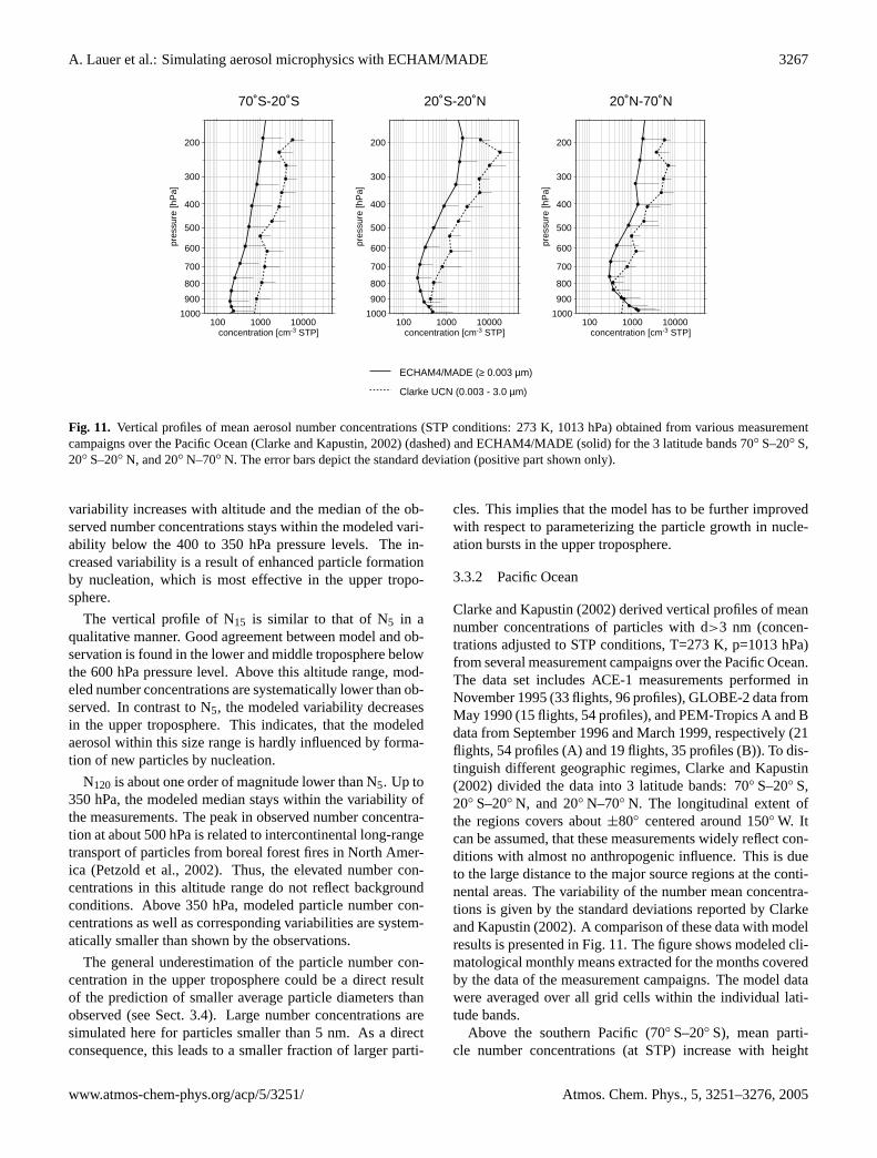
3.3.2 Pacific Ocean
Clarke and Kapustin(2002) derived vertical profiles of meannumber concentrations of particles with d>3 nm (concen-trations adjusted to STP conditions, T=273 K, p=1013 hPa)from several measurement campaigns over the Pacific Ocean.The data set includes ACE-1 measurements performed inNovember 1995 (33 flights, 96 profiles), GLOBE-2 data fromMay 1990 (15 flights, 54 profiles), and PEM-Tropics A and Bdata from September 1996 and March 1999, respectively (21flights, 54 profiles (A) and 19 flights, 35 profiles (B)). To dis-tinguish different geographic regimes,Clarke and Kapustin(2002) divided the data into 3 latitude bands: 70◦ S–20◦ S,20◦ S–20◦ N, and 20◦ N–70◦ N. The longitudinal extent ofthe regions covers about±80◦ centered around 150◦ W. Itcan be assumed, that these measurements widely reflect con-ditions with almost no anthropogenic influence. This is dueto the large distance to the major source regions at the conti-nental areas. The variability of the number mean concentra-tions is given by the standard deviations reported byClarkeand Kapustin(2002). A comparison of these data with modelresults is presented in Fig.11. The figure shows modeled cli-matological monthly means extracted for the months coveredby the data of the measurement campaigns. The model datawere averaged over all grid cells within the individual lati-tude bands.
Above the southern Pacific (70◦ S–20◦ S), mean parti-cle number concentrations (at STP) increase with height
www.atmos-chem-phys.org/acp/5/3251/ Atmos. Chem. Phys., 5, 3251–3276, 2005

3268 A. Lauer et al.: Simulating aerosol microphysics with ECHAM/MADE
A. Lauer et al.: Simulating aerosol microphysics with ECHAM/MADE 33
10
100
1000
10000
100000
dN/d
ln(d
) [c
m-3
]
0.001 0.01 0.1 1d [µm]
ECHAM4/MADE Median
Melpitz Median
Fig. 12. Typical number size distributions (median) obtained dur-ing a period of 17 months for different weather conditions or airmass types, respectively, in Melpitz (Birmili et al., 2001) (dashed)and the corresponding climatological annual median calculated byECHAM4/MADE (solid). The shaded areas indicate the 25%- and75%- and the 5%- and 95%-percentiles of the model results.
www.atmos-chem-phys.org/acp/0000/0001/ Atmos. Chem. Phys., 0000, 0001–36, 2005
Fig. 12. Typical number size distributions (median) obtained dur-ing a period of 17 months for different weather conditions or airmass types, respectively, in Melpitz (Birmili et al., 2001) (dashed)and the corresponding climatological annual median calculated byECHAM4/MADE (solid). The shaded areas indicate the 25%- and75%- and the 5%- and 95%-percentiles of the model results.
by about one order of magnitude between the surfaceand altitudes around the 200 hPa level. This is shownboth by the model results and the observations. How-ever, ECHAM4/MADE systematically underestimates parti-cle number concentration by the factor 3.7 (overall average).This might be related to sea salt particles or mineral dust inthe size range of the Aitken mode, which are currently nottaken into account by the model, but might become impor-tant under clean remote conditions.
In the northern hemisphere (20◦ N–70◦ N), a much betterquantitative agreement between model and measurements isachieved. On overall average, the particle number concen-tration is underestimated by a factor of 1.4 by the model.In contrast to the southern hemisphere, there’s no systematicover- or underestimation by the model throughout the wholetroposphere. Up to about 400 hPa, model and observationare conformable within the variability of the number con-centrations. Nevertheless, the particle number concentrationis systematically underestimated by the model in the uppertroposphere. Thus, the major characteristics of differencesbetween modeled and observed profiles follow the character-istics found in the intercomparison of ECHAM4/MADE re-sults with vertical profiles observed during LACE in CentralEurope (Sect.3.3.1).
The observed and simulated tropical profiles (20◦ S–20◦ N) show good agreement in the lower troposphere upto about 900 hPa. In the middle and upper troposphere,the model systematically underestimates the particle numberconcentration. Both measurements and simulation show anincrease in number concentration between 700 and 200 hPaof about one order of magnitude. On overall average, theobserved number concentrations are about 2.8 times higherthan calculated by the model.
This comparison shows that ECHAM4/MADE performsreasonably well in the northern hemispheric lower tropo-sphere, but systematically underestimates particle numberconcentration in the upper troposphere and lowermost strato-sphere as well as in the lower troposphere of clean remote
areas such as the southern hemisphere. Such a behaviorof the model is also suggested by comparison with aircraftmeasurements (not shown) obtained during the project Inter-hemispheric Differences in Cirrus Properties from Anthro-pogenic Emissions (INCA) (Minikin et al., 2003). Hence themodel has to be improved for application in remote areas andhigher altitudes. The latter particularly concerns the repre-sentation of nucleation, the most important source of newparticle number concentration in the upper troposphere, andthe growth of these fresh particles into the size range of theAitken mode.
3.3.3 Particle number concentration – conclusions
Both the order of magnitude of the particle number concen-tration and the difference between the individual size classes(modes) is captured by ECHAM4/MADE correctly. Thequalitative differences between northern and southern hemi-sphere and between clean and polluted conditions are repro-duced by the model. Modeled and observed number con-centrations are in good agreement in the lower and mid-troposphere, in particular in polluted continental areas. How-ever, the model underestimates particle numbers in the up-per troposphere as well as for clean remote conditions suchas for marine conditions in the southern hemispheric bound-ary layer. A more detailed analysis of the model data showsthat the average diameter of the upper tropospheric particlescalculated by the model is smaller than found during mea-surements. This results in many particles slightly below thedetection limit of the measurements. A slight reduction ofthe lower limit (diameter) when calculating particle num-ber from the model data (above a certain threshold dime-ter) would result in significantly enhanced number concen-trations. This is the case in particular for Aitken mode par-ticles. As concluded in Sect.3.3.1 this again suggests thatthe model has to be improved especially with respect to therepresentation of the particle growth following efficient nu-cleation events.
3.4 Size distribution
3.4.1 Central Europe
Melpitz
A time series of measurements of the aerosol number sizedistribution at the German site Melpitz (51◦32′ N, 12◦56′ O)has been statistically analyzed byBirmili et al. (2001). Thedata span a period of 17 months ranging from March 1996to August 1997. Observed air mass types have been clas-sified by origin and major characteristics. For each type,log-normal size distributions for up to 5 modes were fittedto the measurements, covering the size range from 3 nmto 0.8 µm. A nucleation mode (≈3–9 nm), an aged nucle-ation mode (≈9–30 nm), the Aitken mode (≈30–110 nm),the accumulation mode (>110 nm), and (occasionally) a sec-
Atmos. Chem. Phys., 5, 3251–3276, 2005 www.atmos-chem-phys.org/acp/5/3251/
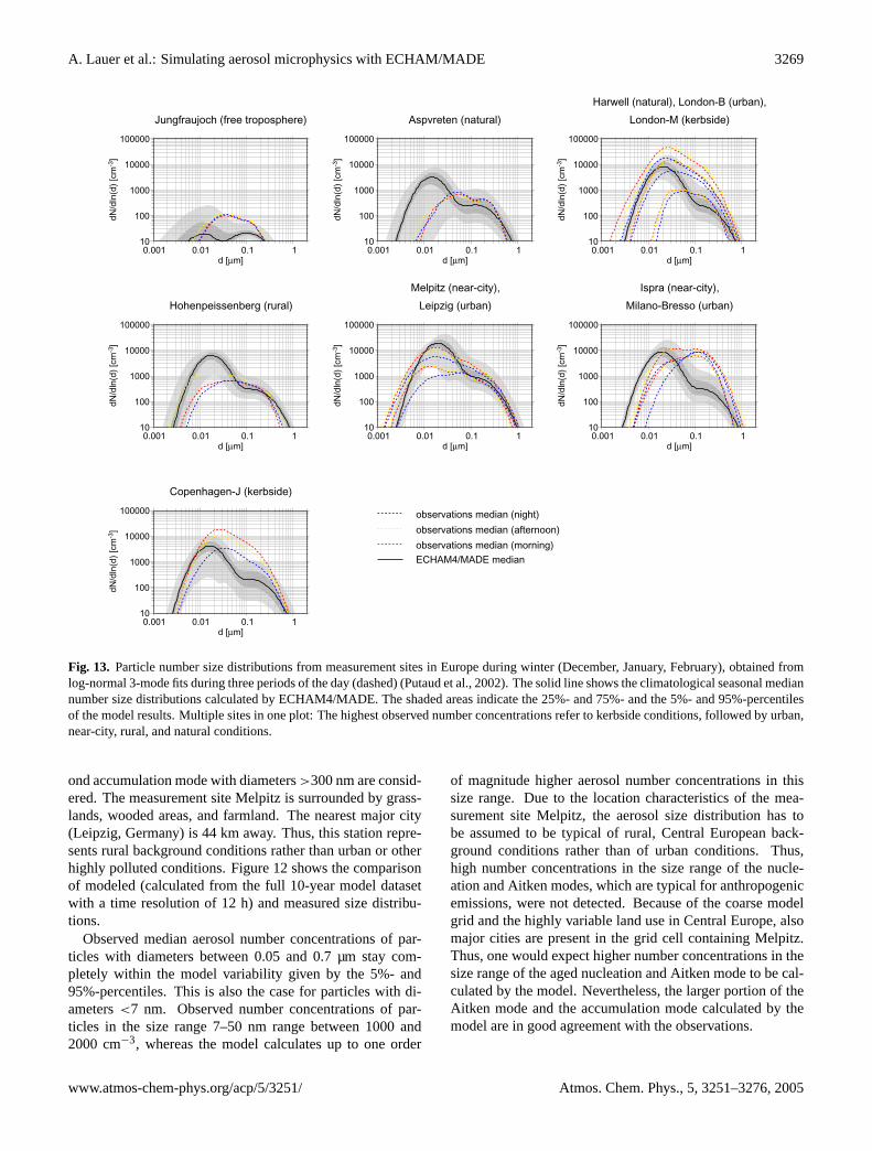
A. Lauer et al.: Simulating aerosol microphysics with ECHAM/MADE 3269
34 A. Lauer et al.: Simulating aerosol microphysics with ECHAM/MADE
10
100
1000
10000
100000
dN/d
ln(d
) [c
m-3
]
0.001 0.01 0.1 1d [µm]
Jungfraujoch (free troposphere)
10
100
1000
10000
100000
dN/d
ln(d
) [c
m-3
]
0.001 0.01 0.1 1d [µm]
Aspvreten (natural)
10
100
1000
10000
100000
dN/d
ln(d
) [c
m-3
]
0.001 0.01 0.1 1d [µm]
Harwell (natural), London-B (urban),
London-M (kerbside)
10
100
1000
10000
100000
dN/d
ln(d
) [c
m-3
]
0.001 0.01 0.1 1d [µm]
Hohenpeissenberg (rural)
10
100
1000
10000
100000dN
/dln
(d)
[cm
-3]
0.001 0.01 0.1 1d [µm]
Melpitz (near-city),
Leipzig (urban)
10
100
1000
10000
100000
dN/d
ln(d
) [c
m-3
]
0.001 0.01 0.1 1d [µm]
Ispra (near-city),
Milano-Bresso (urban)
10
100
1000
10000
100000
dN/d
ln(d
) [c
m-3
]
0.001 0.01 0.1 1d [µm]
Copenhagen-J (kerbside)
ECHAM4/MADE median
observations median (morning)
observations median (afternoon)
observations median (night)
Fig. 13. Particle number size distributions from measurementsites in Europe during winter (December, January, February), ob-tained from log-normal 3-mode fits during three periods of the day(dashed) (Putaud et al., 2002). The solid line shows the clima-tological seasonal median number size distributions calculated byECHAM4/MADE. The shaded areas indicate the 25%- and 75%-and the 5%- and 95%-percentiles of the model results. Multiplesites in one plot: The highest observed number concentrations re-fer to kerbside conditions, followed by urban, near-city, rural, andnatural conditions.
Atmos. Chem. Phys., 0000, 0001–36, 2005 www.atmos-chem-phys.org/acp/0000/0001/
Fig. 13. Particle number size distributions from measurement sites in Europe during winter (December, January, February), obtained fromlog-normal 3-mode fits during three periods of the day (dashed) (Putaud et al., 2002). The solid line shows the climatological seasonal mediannumber size distributions calculated by ECHAM4/MADE. The shaded areas indicate the 25%- and 75%- and the 5%- and 95%-percentilesof the model results. Multiple sites in one plot: The highest observed number concentrations refer to kerbside conditions, followed by urban,near-city, rural, and natural conditions.
ond accumulation mode with diameters>300 nm are consid-ered. The measurement site Melpitz is surrounded by grass-lands, wooded areas, and farmland. The nearest major city(Leipzig, Germany) is 44 km away. Thus, this station repre-sents rural background conditions rather than urban or otherhighly polluted conditions. Figure12 shows the comparisonof modeled (calculated from the full 10-year model datasetwith a time resolution of 12 h) and measured size distribu-tions.
Observed median aerosol number concentrations of par-ticles with diameters between 0.05 and 0.7 µm stay com-pletely within the model variability given by the 5%- and95%-percentiles. This is also the case for particles with di-ameters<7 nm. Observed number concentrations of par-ticles in the size range 7–50 nm range between 1000 and2000 cm−3, whereas the model calculates up to one order
of magnitude higher aerosol number concentrations in thissize range. Due to the location characteristics of the mea-surement site Melpitz, the aerosol size distribution has tobe assumed to be typical of rural, Central European back-ground conditions rather than of urban conditions. Thus,high number concentrations in the size range of the nucle-ation and Aitken modes, which are typical for anthropogenicemissions, were not detected. Because of the coarse modelgrid and the highly variable land use in Central Europe, alsomajor cities are present in the grid cell containing Melpitz.Thus, one would expect higher number concentrations in thesize range of the aged nucleation and Aitken mode to be cal-culated by the model. Nevertheless, the larger portion of theAitken mode and the accumulation mode calculated by themodel are in good agreement with the observations.
www.atmos-chem-phys.org/acp/5/3251/ Atmos. Chem. Phys., 5, 3251–3276, 2005
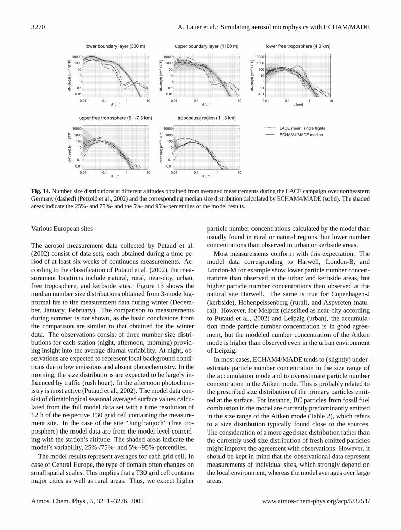
3270 A. Lauer et al.: Simulating aerosol microphysics with ECHAM/MADE
A. Lauer et al.: Simulating aerosol microphysics with ECHAM/MADE 35
lower boundary layer (300 m)
0.01
0.1
1
10
100
1000
10000
dN/d
ln(d
) [c
m-3
ST
P]
0.01 0.1 1 10d [µm]
upper boundary layer (1100 m)
0.01
0.1
1
10
100
1000
10000
dN/d
ln(d
) [c
m-3
ST
P]
0.01 0.1 1 10d [µm]
lower free troposphere (4.0 km)
0.01
0.1
1
10
100
1000
10000
dN/d
ln(d
) [c
m-3
ST
P]
0.01 0.1 1 10d [µm]
upper free troposphere (6.1-7.3 km)
0.01
0.1
1
10
100
1000
10000
dN/d
ln(d
) [c
m-3
ST
P]
0.01 0.1 1 10d [µm]
tropopause region (11.3 km)
0.01
0.1
1
10
100
1000
10000
dN/d
ln(d
) [c
m-3
ST
P]
0.01 0.1 1 10d [µm]
ECHAM4/MADE median
LACE mean, single flights
Fig. 14. Number size distributions at different altitudes obtainedfrom averaged measurements during the LACE campaign overnortheastern Germany (dashed) (Petzold et al., 2002) and the corre-sponding median size distribution calculated by ECHAM4/MADE(solid). The shaded areas indicate the 25%- and 75%- and the 5%-and 95%-percentiles of the model results.
www.atmos-chem-phys.org/acp/0000/0001/ Atmos. Chem. Phys., 0000, 0001–36, 2005
Fig. 14.Number size distributions at different altitudes obtained from averaged measurements during the LACE campaign over northeasternGermany (dashed) (Petzold et al., 2002) and the corresponding median size distribution calculated by ECHAM4/MADE (solid). The shadedareas indicate the 25%- and 75%- and the 5%- and 95%-percentiles of the model results.
Various European sites
The aerosol measurement data collected byPutaud et al.(2002) consist of data sets, each obtained during a time pe-riod of at least six weeks of continuous measurements. Ac-cording to the classification ofPutaud et al.(2002), the mea-surement locations include natural, rural, near-city, urban,free troposphere, and kerbside sites. Figure13 shows themedian number size distributions obtained from 3-mode log-normal fits to the measurement data during winter (Decem-ber, January, February). The comparison to measurementsduring summer is not shown, as the basic conclusions fromthe comparison are similar to that obtained for the winterdata. The observations consist of three number size distri-butions for each station (night, afternoon, morning) provid-ing insight into the average diurnal variability. At night, ob-servations are expected to represent local background condi-tions due to low emissions and absent photochemistry. In themorning, the size distributions are expected to be largely in-fluenced by traffic (rush hour). In the afternoon photochem-istry is most active (Putaud et al., 2002). The model data con-sist of climatological seasonal averaged surface values calcu-lated from the full model data set with a time resolution of12 h of the respective T30 grid cell containing the measure-ment site. In the case of the site “Jungfraujoch” (free tro-posphere) the model data are from the model level coincid-ing with the station’s altitude. The shaded areas indicate themodel’s variability, 25%-/75%- and 5%-/95%-percentiles.
The model results represent averages for each grid cell. Incase of Central Europe, the type of domain often changes onsmall spatial scales. This implies that a T30 grid cell containsmajor cities as well as rural areas. Thus, we expect higher
particle number concentrations calculated by the model thanusually found in rural or natural regions, but lower numberconcentrations than observed in urban or kerbside areas.
Most measurements conform with this expectation. Themodel data corresponding to Harwell, London-B, andLondon-M for example show lower particle number concen-trations than observed in the urban and kerbside areas, buthigher particle number concentrations than observed at thenatural site Harwell. The same is true for Copenhagen-J(kerbside), Hohenpeissenberg (rural), and Aspvreten (natu-ral). However, for Melptiz (classified as near-city accordingto Putaud et al., 2002) and Leipzig (urban), the accumula-tion mode particle number concentration is in good agree-ment, but the modeled number concentration of the Aitkenmode is higher than observed even in the urban environmentof Leipzig.
In most cases, ECHAM4/MADE tends to (slightly) under-estimate particle number concentration in the size range ofthe accumulation mode and to overestimate particle numberconcentration in the Aitken mode. This is probably related tothe prescribed size distribution of the primary particles emit-ted at the surface. For instance, BC particles from fossil fuelcombustion in the model are currently predominantly emittedin the size range of the Aitken mode (Table2), which refersto a size distribution typically found close to the sources.The consideration of a more aged size distribution rather thanthe currently used size distribution of fresh emitted particlesmight improve the agreement with observations. However, itshould be kept in mind that the observational data representmeasurements of individual sites, which strongly depend onthe local environment, whereas the model averages over largeareas.
Atmos. Chem. Phys., 5, 3251–3276, 2005 www.atmos-chem-phys.org/acp/5/3251/
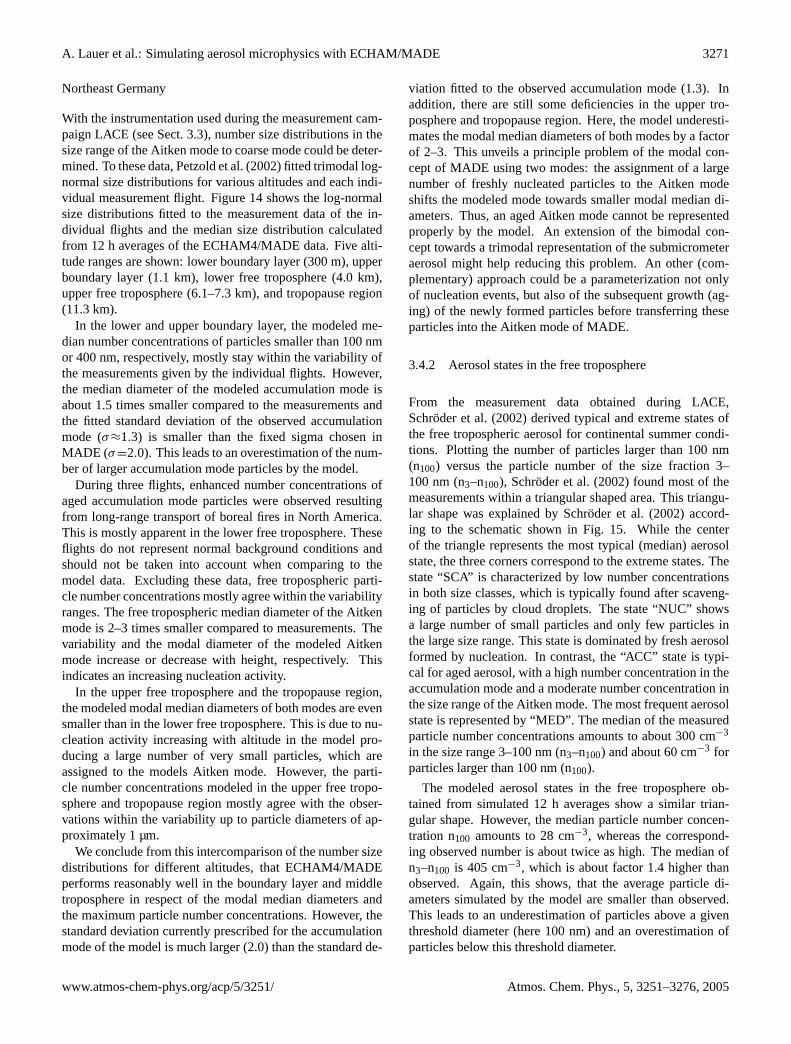
A. Lauer et al.: Simulating aerosol microphysics with ECHAM/MADE 3271
Northeast Germany
With the instrumentation used during the measurement cam-paign LACE (see Sect.3.3), number size distributions in thesize range of the Aitken mode to coarse mode could be deter-mined. To these data,Petzold et al.(2002) fitted trimodal log-normal size distributions for various altitudes and each indi-vidual measurement flight. Figure14 shows the log-normalsize distributions fitted to the measurement data of the in-dividual flights and the median size distribution calculatedfrom 12 h averages of the ECHAM4/MADE data. Five alti-tude ranges are shown: lower boundary layer (300 m), upperboundary layer (1.1 km), lower free troposphere (4.0 km),upper free troposphere (6.1–7.3 km), and tropopause region(11.3 km).
In the lower and upper boundary layer, the modeled me-dian number concentrations of particles smaller than 100 nmor 400 nm, respectively, mostly stay within the variability ofthe measurements given by the individual flights. However,the median diameter of the modeled accumulation mode isabout 1.5 times smaller compared to the measurements andthe fitted standard deviation of the observed accumulationmode (σ≈1.3) is smaller than the fixed sigma chosen inMADE (σ=2.0). This leads to an overestimation of the num-ber of larger accumulation mode particles by the model.
During three flights, enhanced number concentrations ofaged accumulation mode particles were observed resultingfrom long-range transport of boreal fires in North America.This is mostly apparent in the lower free troposphere. Theseflights do not represent normal background conditions andshould not be taken into account when comparing to themodel data. Excluding these data, free tropospheric parti-cle number concentrations mostly agree within the variabilityranges. The free tropospheric median diameter of the Aitkenmode is 2–3 times smaller compared to measurements. Thevariability and the modal diameter of the modeled Aitkenmode increase or decrease with height, respectively. Thisindicates an increasing nucleation activity.
In the upper free troposphere and the tropopause region,the modeled modal median diameters of both modes are evensmaller than in the lower free troposphere. This is due to nu-cleation activity increasing with altitude in the model pro-ducing a large number of very small particles, which areassigned to the models Aitken mode. However, the parti-cle number concentrations modeled in the upper free tropo-sphere and tropopause region mostly agree with the obser-vations within the variability up to particle diameters of ap-proximately 1 µm.
We conclude from this intercomparison of the number sizedistributions for different altitudes, that ECHAM4/MADEperforms reasonably well in the boundary layer and middletroposphere in respect of the modal median diameters andthe maximum particle number concentrations. However, thestandard deviation currently prescribed for the accumulationmode of the model is much larger (2.0) than the standard de-
viation fitted to the observed accumulation mode (1.3). Inaddition, there are still some deficiencies in the upper tro-posphere and tropopause region. Here, the model underesti-mates the modal median diameters of both modes by a factorof 2–3. This unveils a principle problem of the modal con-cept of MADE using two modes: the assignment of a largenumber of freshly nucleated particles to the Aitken modeshifts the modeled mode towards smaller modal median di-ameters. Thus, an aged Aitken mode cannot be representedproperly by the model. An extension of the bimodal con-cept towards a trimodal representation of the submicrometeraerosol might help reducing this problem. An other (com-plementary) approach could be a parameterization not onlyof nucleation events, but also of the subsequent growth (ag-ing) of the newly formed particles before transferring theseparticles into the Aitken mode of MADE.
3.4.2 Aerosol states in the free troposphere
From the measurement data obtained during LACE,Schroder et al.(2002) derived typical and extreme states ofthe free tropospheric aerosol for continental summer condi-tions. Plotting the number of particles larger than 100 nm(n100) versus the particle number of the size fraction 3–100 nm (n3–n100), Schroder et al.(2002) found most of themeasurements within a triangular shaped area. This triangu-lar shape was explained bySchroder et al.(2002) accord-ing to the schematic shown in Fig.15. While the centerof the triangle represents the most typical (median) aerosolstate, the three corners correspond to the extreme states. Thestate “SCA” is characterized by low number concentrationsin both size classes, which is typically found after scaveng-ing of particles by cloud droplets. The state “NUC” showsa large number of small particles and only few particles inthe large size range. This state is dominated by fresh aerosolformed by nucleation. In contrast, the “ACC” state is typi-cal for aged aerosol, with a high number concentration in theaccumulation mode and a moderate number concentration inthe size range of the Aitken mode. The most frequent aerosolstate is represented by “MED”. The median of the measuredparticle number concentrations amounts to about 300 cm−3
in the size range 3–100 nm (n3–n100) and about 60 cm−3 forparticles larger than 100 nm (n100).
The modeled aerosol states in the free troposphere ob-tained from simulated 12 h averages show a similar trian-gular shape. However, the median particle number concen-tration n100 amounts to 28 cm−3, whereas the correspond-ing observed number is about twice as high. The median ofn3–n100 is 405 cm−3, which is about factor 1.4 higher thanobserved. Again, this shows, that the average particle di-ameters simulated by the model are smaller than observed.This leads to an underestimation of particles above a giventhreshold diameter (here 100 nm) and an overestimation ofparticles below this threshold diameter.
www.atmos-chem-phys.org/acp/5/3251/ Atmos. Chem. Phys., 5, 3251–3276, 2005
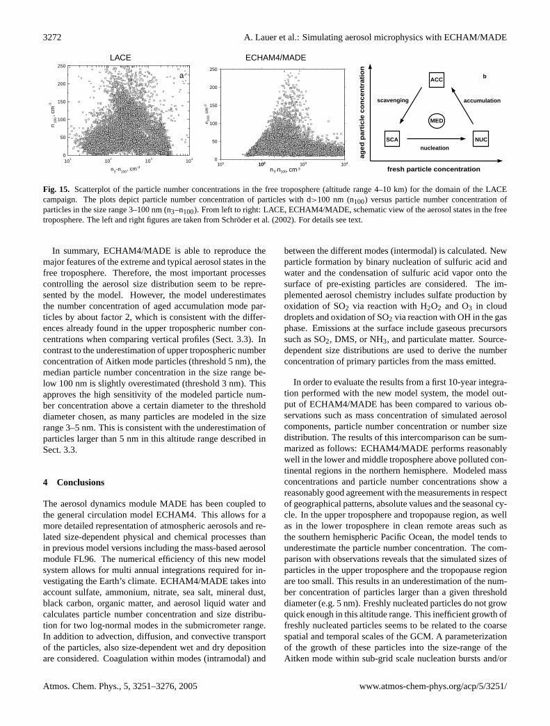
3272 A. Lauer et al.: Simulating aerosol microphysics with ECHAM/MADE
LACE ECHAM4/MADE
0
50
100
150
200
250
101
102
103
104
a
n 100
, cm
-3
n3-n100, cm-3
0
50
100
150
200
250
n 100
, cm
-3
101 102102 103 104
n 3-n100, cm-3 fresh particle concentration
ag
ed
part
icle
co
ncen
trati
on
nucleation
accumulationscavenging
NUCSCA
ACC
MED
b
Fig. 15. Scatterplot of the particle number concentrations in the free troposphere (altitude range 4–10 km) for the domain of the LACEcampaign. The plots depict particle number concentration of particles with d>100 nm (n100) versus particle number concentration ofparticles in the size range 3–100 nm (n3–n100). From left to right: LACE, ECHAM4/MADE, schematic view of the aerosol states in the freetroposphere. The left and right figures are taken fromSchroder et al.(2002). For details see text.
In summary, ECHAM4/MADE is able to reproduce themajor features of the extreme and typical aerosol states in thefree troposphere. Therefore, the most important processescontrolling the aerosol size distribution seem to be repre-sented by the model. However, the model underestimatesthe number concentration of aged accumulation mode par-ticles by about factor 2, which is consistent with the differ-ences already found in the upper tropospheric number con-centrations when comparing vertical profiles (Sect.3.3). Incontrast to the underestimation of upper tropospheric numberconcentration of Aitken mode particles (threshold 5 nm), themedian particle number concentration in the size range be-low 100 nm is slightly overestimated (threshold 3 nm). Thisapproves the high sensitivity of the modeled particle num-ber concentration above a certain diameter to the thresholddiameter chosen, as many particles are modeled in the sizerange 3–5 nm. This is consistent with the underestimation ofparticles larger than 5 nm in this altitude range described inSect.3.3.
4 Conclusions
The aerosol dynamics module MADE has been coupled tothe general circulation model ECHAM4. This allows for amore detailed representation of atmospheric aerosols and re-lated size-dependent physical and chemical processes thanin previous model versions including the mass-based aerosolmodule FL96. The numerical efficiency of this new modelsystem allows for multi annual integrations required for in-vestigating the Earth’s climate. ECHAM4/MADE takes intoaccount sulfate, ammonium, nitrate, sea salt, mineral dust,black carbon, organic matter, and aerosol liquid water andcalculates particle number concentration and size distribu-tion for two log-normal modes in the submicrometer range.In addition to advection, diffusion, and convective transportof the particles, also size-dependent wet and dry depositionare considered. Coagulation within modes (intramodal) and
between the different modes (intermodal) is calculated. Newparticle formation by binary nucleation of sulfuric acid andwater and the condensation of sulfuric acid vapor onto thesurface of pre-existing particles are considered. The im-plemented aerosol chemistry includes sulfate production byoxidation of SO2 via reaction with H2O2 and O3 in clouddroplets and oxidation of SO2 via reaction with OH in the gasphase. Emissions at the surface include gaseous precursorssuch as SO2, DMS, or NH3, and particulate matter. Source-dependent size distributions are used to derive the numberconcentration of primary particles from the mass emitted.
In order to evaluate the results from a first 10-year integra-tion performed with the new model system, the model out-put of ECHAM4/MADE has been compared to various ob-servations such as mass concentration of simulated aerosolcomponents, particle number concentration or number sizedistribution. The results of this intercomparison can be sum-marized as follows: ECHAM4/MADE performs reasonablywell in the lower and middle troposphere above polluted con-tinental regions in the northern hemisphere. Modeled massconcentrations and particle number concentrations show areasonably good agreement with the measurements in respectof geographical patterns, absolute values and the seasonal cy-cle. In the upper troposphere and tropopause region, as wellas in the lower troposphere in clean remote areas such asthe southern hemispheric Pacific Ocean, the model tends tounderestimate the particle number concentration. The com-parison with observations reveals that the simulated sizes ofparticles in the upper troposphere and the tropopause regionare too small. This results in an underestimation of the num-ber concentration of particles larger than a given thresholddiameter (e.g. 5 nm). Freshly nucleated particles do not growquick enough in this altitude range. This inefficient growth offreshly nucleated particles seems to be related to the coarsespatial and temporal scales of the GCM. A parameterizationof the growth of these particles into the size-range of theAitken mode within sub-grid scale nucleation bursts and/or
Atmos. Chem. Phys., 5, 3251–3276, 2005 www.atmos-chem-phys.org/acp/5/3251/
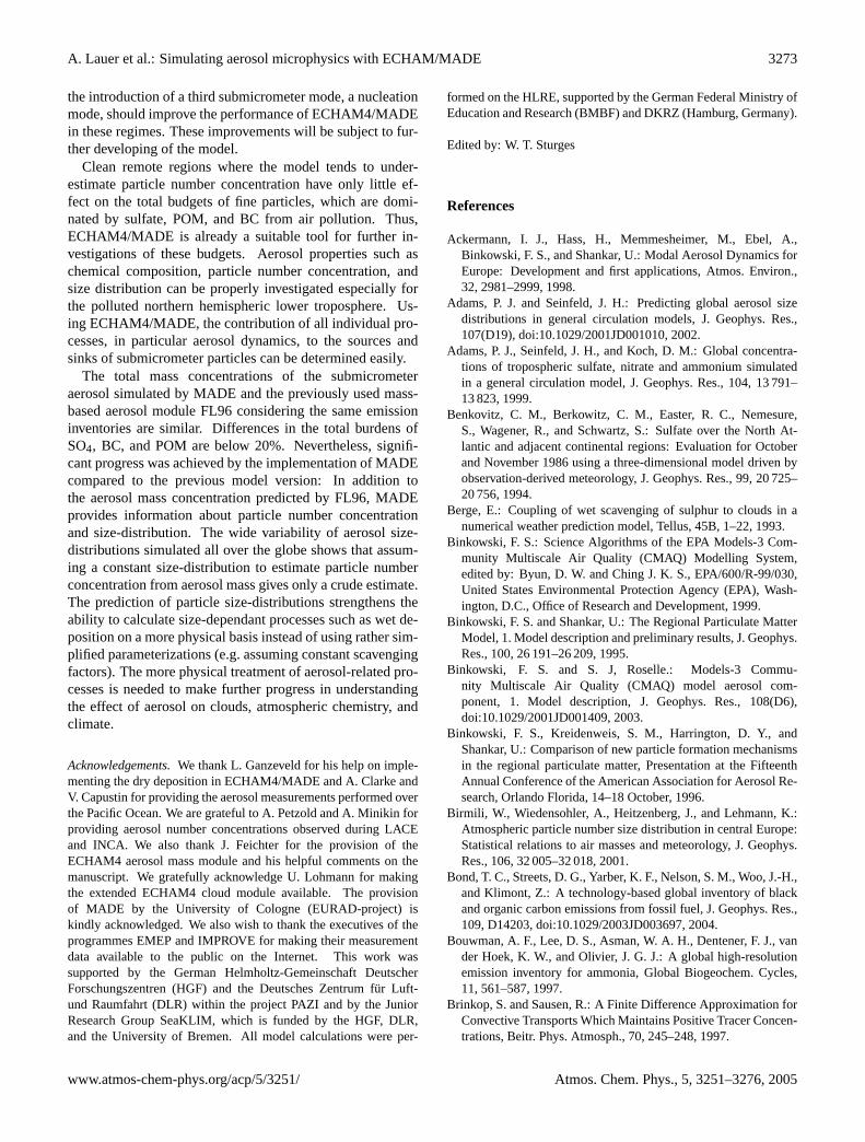
A. Lauer et al.: Simulating aerosol microphysics with ECHAM/MADE 3273
the introduction of a third submicrometer mode, a nucleationmode, should improve the performance of ECHAM4/MADEin these regimes. These improvements will be subject to fur-ther developing of the model.
Clean remote regions where the model tends to under-estimate particle number concentration have only little ef-fect on the total budgets of fine particles, which are domi-nated by sulfate, POM, and BC from air pollution. Thus,ECHAM4/MADE is already a suitable tool for further in-vestigations of these budgets. Aerosol properties such aschemical composition, particle number concentration, andsize distribution can be properly investigated especially forthe polluted northern hemispheric lower troposphere. Us-ing ECHAM4/MADE, the contribution of all individual pro-cesses, in particular aerosol dynamics, to the sources andsinks of submicrometer particles can be determined easily.
The total mass concentrations of the submicrometeraerosol simulated by MADE and the previously used mass-based aerosol module FL96 considering the same emissioninventories are similar. Differences in the total burdens ofSO4, BC, and POM are below 20%. Nevertheless, signifi-cant progress was achieved by the implementation of MADEcompared to the previous model version: In addition tothe aerosol mass concentration predicted by FL96, MADEprovides information about particle number concentrationand size-distribution. The wide variability of aerosol size-distributions simulated all over the globe shows that assum-ing a constant size-distribution to estimate particle numberconcentration from aerosol mass gives only a crude estimate.The prediction of particle size-distributions strengthens theability to calculate size-dependant processes such as wet de-position on a more physical basis instead of using rather sim-plified parameterizations (e.g. assuming constant scavengingfactors). The more physical treatment of aerosol-related pro-cesses is needed to make further progress in understandingthe effect of aerosol on clouds, atmospheric chemistry, andclimate.
Acknowledgements.We thank L. Ganzeveld for his help on imple-menting the dry deposition in ECHAM4/MADE and A. Clarke andV. Capustin for providing the aerosol measurements performed overthe Pacific Ocean. We are grateful to A. Petzold and A. Minikin forproviding aerosol number concentrations observed during LACEand INCA. We also thank J. Feichter for the provision of theECHAM4 aerosol mass module and his helpful comments on themanuscript. We gratefully acknowledge U. Lohmann for makingthe extended ECHAM4 cloud module available. The provisionof MADE by the University of Cologne (EURAD-project) iskindly acknowledged. We also wish to thank the executives of theprogrammes EMEP and IMPROVE for making their measurementdata available to the public on the Internet. This work wassupported by the German Helmholtz-Gemeinschaft DeutscherForschungszentren (HGF) and the Deutsches Zentrum fur Luft-und Raumfahrt (DLR) within the project PAZI and by the JuniorResearch Group SeaKLIM, which is funded by the HGF, DLR,and the University of Bremen. All model calculations were per-
formed on the HLRE, supported by the German Federal Ministry ofEducation and Research (BMBF) and DKRZ (Hamburg, Germany).
Edited by: W. T. Sturges
References
Ackermann, I. J., Hass, H., Memmesheimer, M., Ebel, A.,Binkowski, F. S., and Shankar, U.: Modal Aerosol Dynamics forEurope: Development and first applications, Atmos. Environ.,32, 2981–2999, 1998.
Adams, P. J. and Seinfeld, J. H.: Predicting global aerosol sizedistributions in general circulation models, J. Geophys. Res.,107(D19), doi:10.1029/2001JD001010, 2002.
Adams, P. J., Seinfeld, J. H., and Koch, D. M.: Global concentra-tions of tropospheric sulfate, nitrate and ammonium simulatedin a general circulation model, J. Geophys. Res., 104, 13 791–13 823, 1999.
Benkovitz, C. M., Berkowitz, C. M., Easter, R. C., Nemesure,S., Wagener, R., and Schwartz, S.: Sulfate over the North At-lantic and adjacent continental regions: Evaluation for Octoberand November 1986 using a three-dimensional model driven byobservation-derived meteorology, J. Geophys. Res., 99, 20 725–20 756, 1994.
Berge, E.: Coupling of wet scavenging of sulphur to clouds in anumerical weather prediction model, Tellus, 45B, 1–22, 1993.
Binkowski, F. S.: Science Algorithms of the EPA Models-3 Com-munity Multiscale Air Quality (CMAQ) Modelling System,edited by: Byun, D. W. and Ching J. K. S., EPA/600/R-99/030,United States Environmental Protection Agency (EPA), Wash-ington, D.C., Office of Research and Development, 1999.
Binkowski, F. S. and Shankar, U.: The Regional Particulate MatterModel, 1. Model description and preliminary results, J. Geophys.Res., 100, 26 191–26 209, 1995.
Binkowski, F. S. and S. J, Roselle.: Models-3 Commu-nity Multiscale Air Quality (CMAQ) model aerosol com-ponent, 1. Model description, J. Geophys. Res., 108(D6),doi:10.1029/2001JD001409, 2003.
Binkowski, F. S., Kreidenweis, S. M., Harrington, D. Y., andShankar, U.: Comparison of new particle formation mechanismsin the regional particulate matter, Presentation at the FifteenthAnnual Conference of the American Association for Aerosol Re-search, Orlando Florida, 14–18 October, 1996.
Birmili, W., Wiedensohler, A., Heitzenberg, J., and Lehmann, K.:Atmospheric particle number size distribution in central Europe:Statistical relations to air masses and meteorology, J. Geophys.Res., 106, 32 005–32 018, 2001.
Bond, T. C., Streets, D. G., Yarber, K. F., Nelson, S. M., Woo, J.-H.,and Klimont, Z.: A technology-based global inventory of blackand organic carbon emissions from fossil fuel, J. Geophys. Res.,109, D14203, doi:10.1029/2003JD003697, 2004.
Bouwman, A. F., Lee, D. S., Asman, W. A. H., Dentener, F. J., vander Hoek, K. W., and Olivier, J. G. J.: A global high-resolutionemission inventory for ammonia, Global Biogeochem. Cycles,11, 561–587, 1997.
Brinkop, S. and Sausen, R.: A Finite Difference Approximation forConvective Transports Which Maintains Positive Tracer Concen-trations, Beitr. Phys. Atmosph., 70, 245–248, 1997.
www.atmos-chem-phys.org/acp/5/3251/ Atmos. Chem. Phys., 5, 3251–3276, 2005

3274 A. Lauer et al.: Simulating aerosol microphysics with ECHAM/MADE
Chin, M., Rood, R. B., Lin, S.-J., Muller, J.-F., and Thompson,A.: Atmospheric sulfur cycle simulated in the global model GO-CART: Model description and global properties, J. Geophys.Res., 105, 24 671–24 687, 2000.
Chung, S. H. and Seinfeld, J. H.: Global distribution and climateforcing of carbonaceous aerosols, J. Geophys. Res., 107(D19),doi:10.1029/2001JD001397, 2002.
Clarke, A. D. and Kapustin, V. N.: A Pacific Aerosol Survey. PartI: A Decade of Data on Particle Production, Transport, Evolu-tion, and Mixing in the Troposphere, J. Atmos. Sci., 59, 363–382, 2002.
Cooke, W. F. and Wilson, J. J. N.: A global black carbon aerosolmodel, J. Geophys. Res., 101, 19 395–19 409, 1996.
Cooke, W. F., Liousse, C., and Cachier, H.: Construction of a1◦
×1◦ fossil fuel emission data set for carbonaceous aerosol andimplementation and radiative impact in the ECHAM4 model, J.Geophys. Res., 104, 22 137–22 162, 1999.
Dentener, F.: Heterogeneous chemistry in the troposphere, disser-tation, University of Utrech, Netherlands, ISBN 90-393-0317-7,1993.
Ebel, A., Elbern, H., Hass, H., Jakobs, H. J., Memmesheimer, M.,Laube, M., Oberreuter, A., and Piekorz, G.: Simulation of chem-ical transformation and transport of air pollutants with the modelsystem EURAD, Transport and Chemical Transformation of Pol-lutants in the Troposphere, edited by: Borell, P., Borell, P. M.,and Midgley, P., Vol. 7, Tropospheric Modelling and EmissionEstimation, Springer, Berlin, Germany, 27–45, 1997.
EEA (European Environment Agency): Air pollution in Europe1990–2000, ISBN 92-9167-635-7, 2003.
EMEP Co-operative Programme for Monitoring and Evaluation ofthe Long-Range Transmission of Air Pollutants in Europe: Mea-surement of Particular Matter, Status Report 2003, EMEP/CCC-Report 5/2003, edited by: Kahnert, M., Norwegian Institute forAir Research (NILU), Kjeller, Norway, 2003.
Feichter, J. and Roeckner, E.: Nonlinear Aspects of the ClimateResponse to Greenhouse Gas and Aerosol Forcing, J. Clim., 17,2384–2398, 2004.
Feichter, J., Kjellstrom, E., Rodhe, H., Dentener, F., Lelieveld, J.,and Roelofs, G.-J.: Simulation of the tropospheric sulfur cycle ina global climate model, Atmos. Environ., 30, 1693–1707, 1996.
Feichter, J., Lohmann, U., and Schult, I.: The atmospheric sulfurcycle in ECHAM-4 and its impact on the shortwave radiation,Clim. Dyn., 13, 235–246, 1997.
Ganzeveld, L. and Lelieveld, J.: Dry deposition parameterizationin a chemistry general circulation model and its influence onthe distribution of reactive trace gases, J. Geophys. Res., 100,20 999–21 012, 1995.
Ginoux, P., Chin, M., Tegen, I., Prospero, J., Holben, B., Dubovik,O., and Lin, S.-J.: Sources and distributions of dust aerosols sim-ulated with the GOCART model, J. Geophys. Res., 106, 20 255–20 273, 2001.
Gong, S. L. and Barrie, L. A.: Modeling sea-salt aerosols in the at-mosphere, 1. Model development, J. Geophys. Res., 102, 3805–3818, 1997.
Guenther, A., Hewitt, C. N., Erickson, D., et al.: A global model ofnatural volatile organic compound emissions, J. Geophys. Res.,100, 8873–8892, 1995.
Hao, W. M., Liu, M. H., and Crutzen, P. J.: Estimates of annual andregional releases of CO2 and other trace gases to the atmosphere
from fires in the tropics, based on the FAO statistics for the period1975–1980, Fire in the tropical biota, in: Ecosystem processesand global challenges, edited by: Goldammer, J. G., Springer,New York, USA, 440–462, 1990.
Hein, R., Dameris, M., Schnadt, C., Land, C., Grewe, V., Kohler,I., Ponater, M., Sausen, R., Steil, B., Landgraf, J., and Bruhl,C.: Results of an interactively coupled atmospheric chemistry-general circulation model: Comparison with observations, Ann.Geophys., 19, 435–457, 2001,SRef-ID: 1432-0576/ag/2001-19-435.
Hendricks, J., Karcher, B., Dopelheuer, A., Feichter, J., Lohmann,U., and Baumgardner, D.: Simulating the global atmosphericblack carbon cycle: a revisit to the contribution of aircraft emis-sions, Atmos. Chem. Phys., 4, 2521–2541, 2004,SRef-ID: 1680-7324/acp/2004-4-2521.
Henning, S., Weingartner, E., Schmidt, S., Wendisch, M., Gaggeler,H. W., and Baltensperger, U.: Size-dependent aerosol activationat the high-alpine site Jungfraujoch (3580 m a.s.l.), Tellus, 54B,82–95, 2002.
Hess, M., Koepke, P., and Schult, I.: Optical properties of aerosolsand clouds: The software package OPAC, Bull. Am. Meteorol.Soc., 79, 831–844, 1998.
Hildemann, L. M., Markowski, G. R., Jones, M. C., and Cass,G. R.: Submicrometer aerosol mass distributions of emissionsfrom boilers, fireplaces, automobiles, diesel trucks, and meatcooking operations, Aerosol Sci. Technol., 14, 138–152, 1991.
IPCC (Intergovernmental Panel on Climate Change 2001): ClimateChange 2001, The Scientific Basis, Contribution of WorkingGroup I to the Third Assessment Report of the IntergovernmentalPanel on Climate Change, edited by: Houghton, J. T., Ding, Y.,Griggs, D. J., Noguer, M., van der Linden, P. J., Dai, X., Maskell,K., and Johnson, C. A., Cambridge University Press, Cambridge,United Kingdom and New York, USA, 2001.
Jacobson, M. Z.: GATOR-GCMM: A global- trough urban-scaleair pollution and weather forecast model, 1. Model design andtreatment of subgrid soil, vegetation, roads, rooftops, water, seaice and snow, J. Geophys. Res, 106, 5385–5401, 2001.
Jaenicke, R.: Tropospheric aerosols, in: Aerosol-Cloud-Climate In-teractions, edited by: Hobbs, P. V., Academic Press, San Diego,CA, USA, 1–31, 1993.
Kettle, A. J., Andreae, M. O., Amouroux, D., et al.: A preliminaryglobal database of sea surface dimethyl sulfide as a function oflatitude, longitude, and month, EOS Trans. AGU, 77 (46), 417,Fall Meet. Suppl., 1996.
Kim, Y. P., Seinfeld, J. H., and Saxena, P.: Atmospheric gas/aerosolequilibrium I. Thermodynamic model, Aerosol Sci. Technol., 19(2), 157–181, 1993a.
Kim, Y. P., Seinfeld, J. H., and Saxena, P.: Atmospheric gas/aerosolequilibrium II. Analysis of common approximations and activitycoefficient calculation methods, Aerosol Sci. Technol., 19 (2),182–198, 1993b.
Kohler, I., Dameris, M., Ackermann, I., and Hass, H.: Contributionof road traffic emissions to the atmospheric black carbon burdenin the mid-1990s, J. Geophys. Res., 106, 17 997–18 014, 2001.
Koop, T., Luo, B. P., Tsias, A., and Peter, T.: Water activity asthe determinant for homogeneous ice nucleation in aqueous so-lutions, Nature, 406, 611–614, 2000.
Kulmala, M., Laaksonen, A., and Pirjola, L.: Parameterizations forsulfuric acid/water nucleation rates, J. Geophys. Res., 103, 8301–
Atmos. Chem. Phys., 5, 3251–3276, 2005 www.atmos-chem-phys.org/acp/5/3251/

A. Lauer et al.: Simulating aerosol microphysics with ECHAM/MADE 3275
8308, 1998.Liousse, C., Penner, J. E., Chuang, C., Walton, J. J., Eddleman,
H., and Cachier, H.: A global three-dimensional model studyof carbonaceous aerosols, J. Geophys. Res., 101, 19 411–19 432,1996.
Lohmann, U.: Possible Aerosol Effects on Ice Clouds via ContactNucleation, J. Atmos. Sci., 59, 647–656, 2002.
Lohmann, U. and Karcher, B.: First interactive simulationsof cirrus clouds formed by homogeneous freezing in theECHAM general circulation model, J. Geophys. Res., 107(D10),doi:10.1029/2001JD000767, 2002.
Lohmann, U., Feichter, J., Chuang, C. C., and Penner, J. E.: Pre-diction of the number of cloud droplets in the ECHAM GCM, J.Geophys. Res., 104, 9169–9198, 1999.
Malm, W. C., Pitchford, M. L., Scruggs, M., et al.: Spatial andseasonal patterns and temporal variability of haze and its con-stituents in the United States, Report III, Cooperative Institute forResearch in the Atmosphere, Colorado State University, ISSN0737-5352-47, 2000.
Metzger, S. M., Dentener, F. J., Lelieveld, J., and Pandis, S. N.:Gas/aerosol partitioning I, A computationally efficient model, J.Geophys. Res., 107, doi:10.1029/2001JD001102, 2002a.
Metzger, S. M., Dentener, F. J., Jeuken, A., Krol, M., and Lelieveld,J.: Gas/aerosol partitioning II: Global modelling results, J. Geo-phys. Res., 107(D16), doi:10.1029/2001JD001103, 2002b.
Minikin, A., Petzold, A., Strom, J., Krejci, R., Seifert, M., vanVelthoven, P., Schlager, H., and Schumann, U.: Aircraft Obser-vations of the Upper Tropospheric Fine Particle Aerosol in theNorthern and Southern Hemispheres at Midlatitudes, Geophys.Res. Lett., 30, 1503, doi:10.1029/2002GL016458, 2003.
Monahan, E. C., Spiel, D. E., and Davidson, K. L.: A model ofmarine aerosol generation via whitecaps and wave disruption,Oceanic Whitecaps, edited by: Monahan, E. C. and Mac Nio-caill, G., D. Reidel, Norwell, Massachusetts, USA, 1986.
Napari, I., Noppel, M., Vehkamaki, H., and Kulmala, M.: Param-eterization of ternary nucleation rates for H2SO4-NH3-H2O va-pors, J. Geophys. Res., 107(D19), doi:10.1029/2002JD002132,2002.
Nenes A., Pandis, S. N., and Pilinis, C.: ISORROPIA: A new ther-modynamic equilibrium model for multiphase multicomponentinorganic aerosols, Aquat. Geoch., 4, 123–152, 1998.
Penner, J. E., Chuang, C. C., and Grant, K.: Climate forcing by car-bonaceous and sulfate aerosols, Clim. Dyn., 14, 839–851, 1998.
Petzold, A., Fiebig, M., Flentje, H., Keil, A., Leiterer, U.,Schroder, F., Stifter, A., Wendisch, M., and Wendling, P.:Vertical variability of aerosol properties observed at a con-tinental site during LACE 98, J. Geophys. Res., 107(D21),doi:10.1029/2001JD001043, 2002.
Putaud, J.-P., Dingenen, R. V., Baltensperger, U., et al.: A Euro-pean Aerosol Phenomenology, physical and chemical character-istics of particulate matter at kerbside, urban, rural and back-ground sites in Europe, joint research centre, European Commis-sion, EUR 20411 EN, 2002.
Raes, F., Van Dingenen, R., Vignati, E., Wilson, J., Putaud, J.-P.,Seinfeld, J. H., Adams, P.: Formation and cycling of aerosols inthe global troposphere, Atmos. Environ., 34, 4215–4240, 2000.
Rasch, P. J. and Williamson, D. L.: Computational aspects of mois-ture transport in global models of the atmosphere, Quart. J. R.Met. Soc., 116, 1071–1090, 1990.
Roeckner, E., Arpe, K., Bengtsson, L., Christoph, M., Claussen,M., Dumenil, L., Esch, M., Giorgetta, M., Schlese, U., andSchulzweida, U.: The atmospheric general circulation modelECHAM-4: Model description and simulation of present-day cli-mate, Max Planck Institute for Meteorology, Report No. 218,Hamburg, Germany, ISSN 0937-1060, 1996.
Roeckner, E., Bauml, G., Bonaventura, L., Brokopf, R., Esch,M., Giorgetta, M., Hagemann, S., Kirchner, I., Kornblueh,L., Manzini, E., Rhodin, A., Schlese, U., Schulzweida, U.,and Tompkins, A.: The atmospheric general circulation modelECHAM5, Part I: Model description, Max Planck Institute forMeteorology, Report No. 349, Hamburg, Germany, ISSN 0937-1060, 2003.
Saxena, P., Hudischewskyj, A. B., Seigneur, C., and Seinfeld, J. H.:A comparative study of equilibrium approaches to the chemicalcharacterization of secondary aerosols, Atmos. Environ., 20, 7,1471–1483, 1986.
Schell, B., Ackermann, I. J., Hass, H., Binkowski, F. S., and Ebel,A.: Modeling the formation of secondary organic aerosol withina comprehensive air quality model system, J. Geophys. Res.,106(D22), doi:10.1029/2001JD000384, 2001.
Seinfeld, J. H. and Pandis, S. N.: Atmospheric Chemistry andPhysics – From Air Pollution to Climate Change, John Wileyand Sons, Inc., New York, USA, 1998.
Schroder, F., Karcher, B., Fiebig, M., and Petzold, A.: Aerosolstates in the free troposphere at northern midlatitudes, J. Geo-phys. Res., 107(D21), doi:10.1029/2000JD000194, 2002.
Schulz, M., Balkanski, Y. J., Guelle, W., and Dulac, F.: Roleof aerosol size distribution and source location in a three-dimensional simulation of a Saharan dust episode tested againstsatellite-derived optical thickness, J. Geophys. Res., 103,10 579–10 592, 1998.
Slinn, S. A. and Slinn, W. G. N.: Prediction for particle depositionon natural waters, Atmos. Environ., 14, 1013–1016, 1980.
Spiro, P. A., Jacob, D. J., and Logan, J. A.: Global inventory ofsulfur emissions with 1◦×1◦ resolution, J. Geophys. Res., 97,6023–6036, 1992.
Stier, P., Feichter, J., Kinne, S., Kloster, S., Vignati, E., Wilson, J.,Ganzeveld, L., Tegen, I., Werner, M., Balkanski, Y., Schulz, M.,and Boucher, O.: The aerosol-climate model ECHAM5-HAM,Atmos. Chem. Phys., 5, 1125–1156, 2005,SRef-ID: 1680-7324/acp/2005-5-1125.
Takemura, T., Okamoto, H., Maruyama, Y., Numaguti, A., Hig-urashi, A., and Nakajima, T.: Global three-dimensional simula-tion of aerosol optical thickness distribution of various origins, J.Geophys. Res., 105, 17 853–17 873, 2000.
Tanre, D., Geleyn, J.-F., and Slingo, J. M.: First results of theintroduction of an advanced aerosol-radiation interaction in theecmwf low resolution global model, in: Aerosols and Their Cli-matic Effects, edited by: Gerber, H. and Deepak, A., A. Deepak,Hampton, Va, USA, 133–177, 1984.
Tiedtke, M.: A comprehensive mass flux scheme for cumulus pa-rameterization in large-scale models, Mon. Weather Rev., 117,3040–3061, 1989.
Vehkamaki, H., Kulmala, M., Napari, I., Lehtinen, K. E. J.,Timmreck, C., Noppel, M., and Laaksonen, A.: An improvedparameterization for sulfuric acid-water nucleation rates fortropospheric and stratospheric conditions, J. Geophys. Res.,107(D22), doi:10.1029/2002JD002184, 2002.
www.atmos-chem-phys.org/acp/5/3251/ Atmos. Chem. Phys., 5, 3251–3276, 2005

3276 A. Lauer et al.: Simulating aerosol microphysics with ECHAM/MADE
Weber, R. J., Marti, J. J., McMurry, P. H., Eisele, F. L., Tanner,D. J., and Jefferson, A.: Measurements of new particle forma-tion and ultrafine particle growth rates at clean continental site,J. Geophys. Res., 102, 4375–4385, 1997.
Whitby, E. R., McMurray, P. H., Shankar, U., and Binkowski, F. S.:Modal Aerosol Dynamics Modelling, Technical Report 600/3-91/020, (available as NTIS PB91-161729/AS from Natl. Tech.Inf. Serv. Springfield, VA), Atmospheric Research and ExposureAssess. Lab., US Environmental Protection Agency, ResearchTriangle Park, NC, USA, 1991.
Wilson, J., Cuvelier, C., and Raes, F.: A modeling study of globalmixed aerosol fields, J. Geophys. Res., 106, 34 081–34 108,2001.
Atmos. Chem. Phys., 5, 3251–3276, 2005 www.atmos-chem-phys.org/acp/5/3251/