Simulating a Fountain 209

Simulating a Fountain

Lyric P. DoshiJoseph Edgar GonzalezPhilip B. KiddMaggie L. Walker Governor’s School

for Government and International StudiesRichmond, VA

Advisor: John A. Barnes

IntroductionWe establish the mathematical behavior of water droplets emitted from a

fountain and apply this behavior in a computer model to predict the amountof splash and spray produced by a fountain under given conditions.

We combine height and volume of the fountain spray, making both functionsof the speed at which water exits the fountain nozzle. We simulate waterdroplets launched from the fountain, using basic physics to model the effectsof drag, wind, and gravity. The simulation tracks the flight of droplets in theair and records their landing positions, for wind speeds from 0 to 15 m/s andwater speeds from 5 to 30 m/s. It calculates the amount of water spilled outsideof a pool around the fountain, for pool radii from 0 to 40 m.

We design an algorithm for a programmable logic controller, located insidean anemometer, to do a table search to find allowable water speeds for givenpool radius, acceptable water spillage, and wind velocity. We simulated sub-jecting a fountain with a 4-m pool radius to wind speeds from 0 to 3 m/s withan allowable spillage of 5%. We tested the model for accuracy and sensitivityto changes in the base variables.

Problem Analysis

WindThe anemometer measures two main wind factors that affect the fountain:

speed, which affects the force exerted on the water, and direction.

The UMAP Journal 23 (3) (2002) 209–219. c©Copyright 2002 by COMAP, Inc. All rights reserved.Permission to make digital or hard copies of part or all of this work for personal or classroom useis granted without fee provided that copies are not made or distributed for profit or commercialadvantage and that copies bear this notice. Abstracting with credit is permitted, but copyrightsfor components of this work owned by others than COMAP must be honored. To copy otherwise,to republish, to post on servers, or to redistribute to lists requires prior permission from COMAP.

210 The UMAP Journal 23.3 (2002)

FountainThe main components of the fountain are the pool and the nozzle. The

factors associated with the pool are its radius, which remains constant withina trial, and the acceptable level of spillage, which describes the percentage ofwater that may acceptably fall outside of the fountain.

NozzleMajor aspects of the nozzle are the radius of the opening, the angle relative

to the vertical axis (normal axis), and the spread and speed of the water passingthrough it. The angle of the nozzle relative to the vertical axis determines theinitial trajectory of the water. The spread, described in standard deviations fromthe angle of the nozzle, determines the extent to which the initial trajectory ofdroplets differs from the angle of the nozzle. For a given water speed andnozzle radius, the flow of water through the nozzle may be determined from

f = πr2v,

where f is flow, v is the water launch speed, and r is the radius of the nozzle.The radius is constant, so the flow and consequent volume are functions of thespeed, the dominant controllable factor affecting the height of the stream.

Assumptions

. . . about Fountains• The fountain is composed of a single nozzle located at the center of a circular

pool.

• The ledge of the pool is sufficiently high to collect the splatter produced byparticles impacting the surface of the water.

• Fountains with higher streams are more attractive than those with lowerstreams.

. . . about the Nozzle• The nozzle has a fixed radius, but the speed of the water through it can be

controlled.

• The nozzle is perpendicular to the ground.

• The nozzle responds rapidly to input from the anemometer.

• The nozzle produces a normally distributed spread of droplets with a lowstandard deviation.

Simulating a Fountain 211

. . . about Water Droplets• Because the droplets are small and roughly spherical, they may be treated

as spherical.

• The radii of droplets are normally distributed.

• The density of water is unaffected by conditions and therefore remains con-stant among and within droplets.

• The only outside forces exerted on a water droplet are gravity and the forceexerted by the surrounding air, including drag and wind.

• Acceleration due to gravity is the same for all droplets.

• The effect of air perturbations produced by droplets on other droplets isinsignificant.

• All droplets share the same constant drag coefficient.

• Droplet interactions and collisions do not increase the overall energy of thesystem or increase the distance traveled by droplets.

. . . about the Anemometer and Control System• The anemometer and control system can rapidly evaluate the wind speed,

apply a basic formula, and adjust the nozzle in changing wind conditions.

. . . about the Wind• The wind speed is uniform regardless of altitude.

• Wind blows parallel to the ground without turbulence or irregularities.

Basic Description of ModelWater droplets are emitted from the nozzle and follow trajectories affected

by wind and drag. The particles are tracked until they land, including recal-culations of trajectories in case of changes in conditions, such as wind. Thelanding distance from the center of the fountain is recorded. Since the fountainpool is circular, only radial distance is important.

The model ignores wind direction (does not affect a circular fountain pool)and turbulence (insignificant and too complicated to model accurately).

We tested droplet collisions and found that they do not greatly affect thedistance that droplets land from the center of the pool; so we ruled out in-corporating complex interactions into the model. Further physical analysis

212 The UMAP Journal 23.3 (2002)

supported that decision: Because of conservation of energy and momentum, adroplet could not travel significantly farther after a collision.

Finally, we combined fountain height and volume into speed of the waterout of the nozzle, because they are directly determined by the speed.

Our simulation tries all combinations of 11 different water speeds, from 5to 30 m/s (at intervals of 0.5 m/s), with 16 wind speeds, from 0 to 15 m/s (atintervals of 1 m/s). Each combination is run for five trials of 10,000 droplets.Spillage is logged for radii from 0 to 40 m (at intervals of 0.1 m). The five trialsare then averaged to construct an entry in a three-dimensional reference table.

The Underlying MathematicsThe simulation uses basic physics equations to model the flight of water

droplets through the air.Each droplet is acted on by three forces: gravity, drag, and wind. Drag is

calculated from the following equation [Halliday et al. 1993]:

D = 12CρAv2,

where

D is the drag coefficient, an empirically-determined constant dependent mainlyon the shape of an object;

ρ is the density of the fluid through which the object is traveling, in this caseair;

A is the cross-sectional area of the object; and

v = |�v| is the speed of the object relative to the wind.

The drag coefficient of a raindrop is 0.60 and the density of air is about1.2 kg/m3 [Halliday et al. 1993]. Drag acts directly against velocity, so theacceleration vector from drag can be found from Newton’s law �F = m�a as

�a =−D

m

�v

|v| =12CρA|�v|2

m

�v

|�v| =12CρA|�v|

m�v,

where �a is the acceleration vector and m is mass.We factor in gravity by subtracting the acceleration g of gravity at Earth’s

surface, 9.8 m/s2, from the vertical component of the acceleration vector:

�az = −12CρA|�v|

m�vz − g.

Next, we use the acceleration to find velocity, beginning with the expression

d�v

dt= −

12CρA|�v|

m�v = �a.

Simulating a Fountain 213

To circumvent the difficulties of solving a differential equation for each compo-nent of the velocity vector, we use Euler’s method to approximate the velocityat a series of discrete points in time:

d�v

dt= �a, ∆�v ≈ ∆t�a, �v1 ≈ �v0 + ∆t�a0.

We use a similar process to find the position of the droplet, resulting in

�x1 ≈ �x0 + ∆t�v0.

With ∆t = 0.001 s, error from the approximation is virtually zero.Now that we have equations for describing the droplet in flight, we gener-

ate its initial position and velocity. First, we randomly select a value z from astandard Gaussian (normal) distribution (mean 0, standard deviation 1). Wecalculate the angle from a set mean µ and standard deviation σ of the distribu-tion of possible angles as

φ = zσ + µ.

We randomly select another angle θ between 0 and 2π radians to be theangle between the velocity vector and the x-axis.

Thus, the initial velocity vector of the droplet in spherical coordinates is(ρ, θ, φ), where ρ is the magnitude of the velocity. Conversion to rectangularcoordinates yields (ρ sinφ cos θ, ρ sinφ sin θ, ρ cos φ).

We also randomly select a starting location within the nozzle (whose diam-eter is 1 cm) and create a radius for the droplet using a similar sampling froma normal distribution. The mass of the droplet is then

m = 43πr3ρ,

where ρ is the density of water, 998.2 kg/m3 at 20◦ C [Lide 1995]. In the basicsimulation, the φ distribution has a mean of 0 and a standard deviation of π/60radians, and the radius distribution has a mean of 0.0015 m and a standarddeviation of 0.0001 m.

In the basic simulation, the nozzle points straight up; however, we also testthe effect of tilting the nozzle away from the wind. The program first rotatesthe nozzle a set angle away from z-axis (π/18, π/9, or π/6 radians). The initialposition and velocity vectors are changed by the formula for rotating a point tradians about the x-axis, from z towards negative y [Dollins 2001]:

x′

y′

z′

=

1 0 00 cos t − sin t0 sin t cos t

xyz

.

Next, the program rotates the nozzle around the z-axis to point directlyaway from the wind (in spherical coordinates, the θ of the nozzle is equal to

214 The UMAP Journal 23.3 (2002)

that of the wind vector). The formula to rotate a point t radians about the z-axis,from x towards y [Dollins 2001] is

x′

y′

z′

=

cos t − sin t 0sin t cos t 01 0 0

xyz

.

Design of ProgramWe developed a program to simulate the fountain. The program compo-

nent Simulator.class manages interactions among the other components ofthe program. Particle.class describes a water droplet in terms of position,velocity, radius, and mass. Vector3D.class creates and performs functionswith vectors, including setting vector components, adding and subtractingvectors, multiplying vectors by scalars, finding the angle between vectors, andfinding the magnitude of a vector.

Emitter.class creates a fountain by spraying droplets. It considers thenozzle radius, direction, and angle orientations and generates launch angle φand launch location on the nozzle according to the prescribed distributions.

Launch speed is determined by Anemometer.class, which takes the wind-speed reading from the anemometer and sends that plus fountain radius andtolerable spillage percentage to FindingVelocity.class. This latter class doesa table lookup and returns the maximum droplet speed for the spillage per-centage. Anemometer.class then sets the droplet emission speed.

Once a droplet is emitted, its trajectory is updated every iteration usingPhysics.class, which checks Wind.class (which contains a vector of thecurrent wind) in each iteration in calculating an updated trajectory. ThenPhysics.class iterates through the entire collection of particles and computesnew velocities and positions based on the forces acting on them.

The Analyzer.class checks to see if any particles have hit the ground; theirlocations are recorded and they are removed from consideration. It then relaysthis information back to Simulator.class, where it is written to disk.

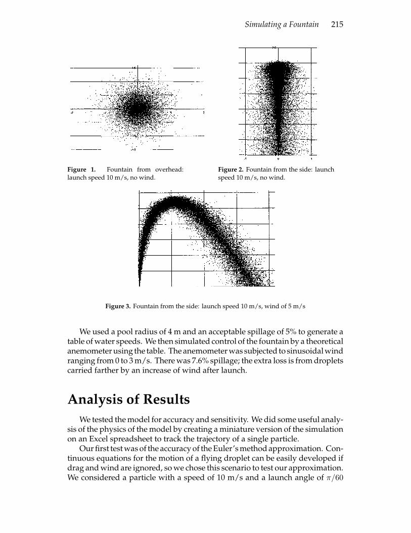
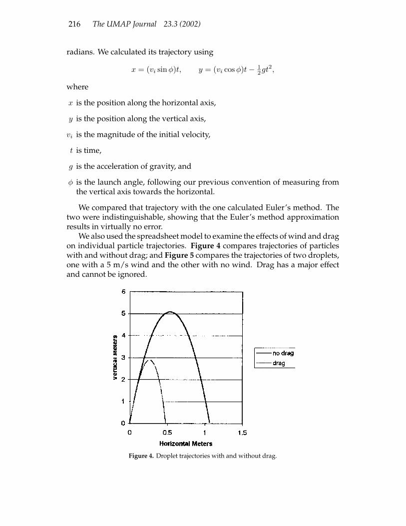
ResultsA program run takes 5 min to model 2 sec of spray (10,000 droplets).Scatterplots showing where droplets land appear uniform and radially sym-

metric (Figure 1); a side profile of the points appears uniformly distributedalong a line and bilaterally symmetric (Figure 2).

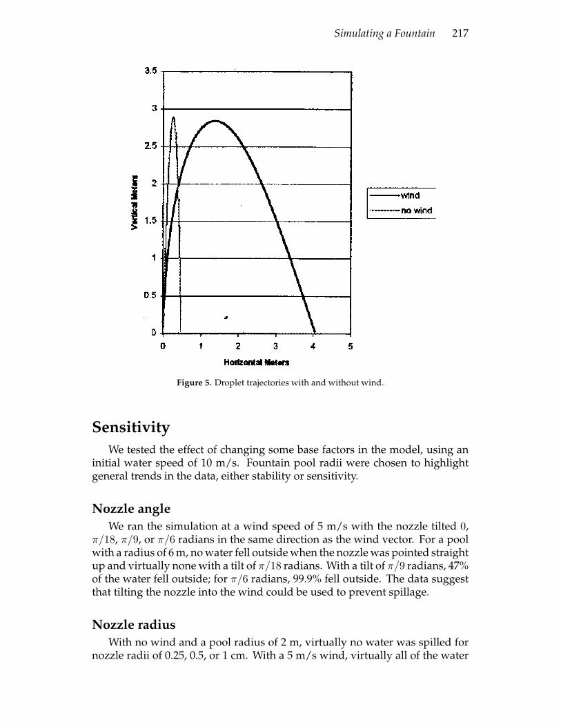
We then introduced wind in the positive x-direction. As expected, thelanding plot and the side profile plot are skewed horizontally (Figure 3).

Figures 1–3 conform very well to the actual appearance of fountains, indi-cating that our model creates an accurate portrait of a real fountain.

Simulating a Fountain 215

Figure 1. Fountain from overhead:launch speed 10 m/s, no wind.

Figure 2. Fountain from the side: launchspeed 10 m/s, no wind.

Figure 3. Fountain from the side: launch speed 10 m/s, wind of 5 m/s

We used a pool radius of 4 m and an acceptable spillage of 5% to generate atable of water speeds. We then simulated control of the fountain by a theoreticalanemometer using the table. The anemometer was subjected to sinusoidal windranging from 0 to 3 m/s. There was 7.6% spillage; the extra loss is from dropletscarried farther by an increase of wind after launch.

Analysis of ResultsWe tested the model for accuracy and sensitivity. We did some useful analy-

sis of the physics of the model by creating a miniature version of the simulationon an Excel spreadsheet to track the trajectory of a single particle.

Our first test was of the accuracy of the Euler’s method approximation. Con-tinuous equations for the motion of a flying droplet can be easily developed ifdrag and wind are ignored, so we chose this scenario to test our approximation.We considered a particle with a speed of 10 m/s and a launch angle of π/60

216 The UMAP Journal 23.3 (2002)

radians. We calculated its trajectory using

x = (vi sinφ)t, y = (vi cos φ)t − 12gt2,

where

x is the position along the horizontal axis,

y is the position along the vertical axis,

vi is the magnitude of the initial velocity,

t is time,

g is the acceleration of gravity, and

φ is the launch angle, following our previous convention of measuring fromthe vertical axis towards the horizontal.

We compared that trajectory with the one calculated Euler’s method. Thetwo were indistinguishable, showing that the Euler’s method approximationresults in virtually no error.

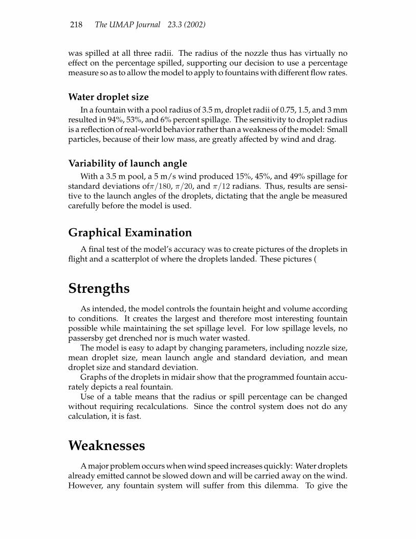
We also used the spreadsheet model to examine the effects of wind and dragon individual particle trajectories. Figure 4 compares trajectories of particleswith and without drag; and Figure 5 compares the trajectories of two droplets,one with a 5 m/s wind and the other with no wind. Drag has a major effectand cannot be ignored.

Figure 4. Droplet trajectories with and without drag.

Simulating a Fountain 217

Figure 5. Droplet trajectories with and without wind.

SensitivityWe tested the effect of changing some base factors in the model, using an

initial water speed of 10 m/s. Fountain pool radii were chosen to highlightgeneral trends in the data, either stability or sensitivity.

Nozzle angleWe ran the simulation at a wind speed of 5 m/s with the nozzle tilted 0,

π/18, π/9, or π/6 radians in the same direction as the wind vector. For a poolwith a radius of 6 m, no water fell outside when the nozzle was pointed straightup and virtually none with a tilt of π/18 radians. With a tilt of π/9 radians, 47%of the water fell outside; for π/6 radians, 99.9% fell outside. The data suggestthat tilting the nozzle into the wind could be used to prevent spillage.

Nozzle radiusWith no wind and a pool radius of 2 m, virtually no water was spilled for

nozzle radii of 0.25, 0.5, or 1 cm. With a 5 m/s wind, virtually all of the water

218 The UMAP Journal 23.3 (2002)

was spilled at all three radii. The radius of the nozzle thus has virtually noeffect on the percentage spilled, supporting our decision to use a percentagemeasure so as to allow the model to apply to fountains with different flow rates.

Water droplet sizeIn a fountain with a pool radius of 3.5 m, droplet radii of 0.75, 1.5, and 3 mm

resulted in 94%, 53%, and 6% percent spillage. The sensitivity to droplet radiusis a reflection of real-world behavior rather than a weakness of the model: Smallparticles, because of their low mass, are greatly affected by wind and drag.

Variability of launch angleWith a 3.5 m pool, a 5 m/s wind produced 15%, 45%, and 49% spillage for

standard deviations ofπ/180, π/20, and π/12 radians. Thus, results are sensi-tive to the launch angles of the droplets, dictating that the angle be measuredcarefully before the model is used.

Graphical ExaminationA final test of the model’s accuracy was to create pictures of the droplets in

flight and a scatterplot of where the droplets landed. These pictures (

StrengthsAs intended, the model controls the fountain height and volume according

to conditions. It creates the largest and therefore most interesting fountainpossible while maintaining the set spillage level. For low spillage levels, nopassersby get drenched nor is much water wasted.

The model is easy to adapt by changing parameters, including nozzle size,mean droplet size, mean launch angle and standard deviation, and meandroplet size and standard deviation.

Graphs of the droplets in midair show that the programmed fountain accu-rately depicts a real fountain.

Use of a table means that the radius or spill percentage can be changedwithout requiring recalculations. Since the control system does not do anycalculation, it is fast.

WeaknessesA major problem occurs when wind speed increases quickly: Water droplets

already emitted cannot be slowed down and will be carried away on the wind.However, any fountain system will suffer from this dilemma. To give the

Simulating a Fountain 219

fountain a small buffer, the radius of the fountain can be set lower than theradius of the pool.

We model the wind as moving parallel to the ground with uniform speed.Real wind may vary with altitude and may blow from above or below thedroplets. We also neglect wind turbulence.

We ignore droplet collisions. Some droplets may combine and then separate,causing slightly more splatter or mist; or the droplets’ collisions may cause moreof them to fall short of their expected trajectories, reducing spillage.

ReferencesDollins, Steven C. 2001. Handy mathematics facts for graphics. http://www.

cs.brown.edu/people/scd/facts . Dated 6 November 2001; accessed 9February 2002.

Halliday, David, Robert Resnick, and Jearl Walker. 1993. Fundamentals ofPhysics. 4th ed. New York: Wiley.

Lide, David R., ed. 1995. CRC Handbook of Chemistry and Physics. Boca Raton,FL: CRC Press.

Yates, Daniel, David Moore, and George McCabe. 1999. The Practice of Statistics.New York: W.H. Freeman.