SIMS2018 CFD Simulation of Solidification of non-Newtonian

SIMS2018 CFD Simulation of Solidification of non-Newtonian

Fluid Flowing in a Complex Geometry Pipeline in Turbulent Flow

Regime

Ludmila Vesjolaja1 Jakub M. Bujalski2 Knut Vaagsaether1 1 Department of Process, Energy and Environmental Technology, University of South-Eastern Norway, Norway,

{ludmila.vesjolaja,knut.vagsather}@usn.no 2 Process Modeling and Control Department, Yara Technology Centre, Norway, [email protected]

Abstract

In this CFD (Computational Fluid Dynamics) study, the

turbulent flow of a non-Newtonian fluid through an

industrial scale transportation pipeline is modelled in

Ansys Fluent®, with a focus on the fluid solidification

due to heat transfer on the pipe walls. The turbulence

was modelled using two different turbulence models: a

standard low-Reynolds-number k-ε turbulence Chan-

Hsieh-Chen (CHC) model and a modified Malin’s

turbulence model. Simulations were performed with

fluid viscosity depending both on the shear rate as well

as on the temperature. However, according to the

simulation results, as long as the inlet fluid velocity is

maintained sufficiently high (turbulent flow), the

occurrence of fluid solidification is not significantly

affected by the viscosity dependence on the temperature.

All turbulence models show fluid solidification on the

pipe walls, and not inside the pipe itself. The standard

CHC model shows more pipe wall zones that are

solidified, while the modified Malin’s turbulence model

shows a more diffusive behavior. The latter model has

an effect on the velocity distribution across the pipeline

in such a way that the fluid flow between the pipelines

become more evenly distributed. The simulation results

of pipe insulation and liquid flow rate, on the fluid

solidification were used to give recommendations of

improvements to avoid blockages in the transportation

pipelines in the industrial process. According to the

simulation results, the use of pipe insulation can

minimize the occurrence of fluid solidification on the

pipe walls.

Keywords: non-Newtonian fluid, turbulent pipe flow,

solidification, Malin turbulence model, CFD

1 Introduction

The solidification of fluids in pipe flows is an important

topic in many practical engineering problems, especially

in manufacturing industries where material phase-

change may occur. The change of phase of the fluid may

cause damages to the pipelines due to blockages that

may eventually lead to unforeseen plant shut downs and

additional cleaning procedures. Due to heat transfer the

phase-change of the fluid usually occurs first on the pipe

wall where a solid phase develops and increases its

radial size with time causing possible pipeline blockages

(Conda et al., 2004; Wei and Güceri, 1988). The

modelling of this phenomenon is very challenging since

they are time-dependent and factors such as flowrate and

temperature directly affect its formation.

Despite the problems caused by fluid solidification in

various engineering processes, very few research works

about fluid solidification have been published in

literature. Early studies devoted to the solidification

phenomena were performed by Hirschberg (1962) and

by Zerkle and Sunderland (1969). In these works, the

solidification of the fluid was studied by assuming a

laminar flow regime at the steady-state (Hirschberg,

1962; Zerkle and Sunderland, 1969). Wei and Güceri

(1988) conducted another significant study where an

attempt was made to develop a numerical model for

describing the solidification in fully developed internal

pipe flows. Almost 20 years later, Conde et al. (2004)

have developed a 2D numerical model for describing the

solidification of water, olive oil and aluminum in

cylindrical ducts. Interestingly, this is the only available

study where solidification in internal pipe flows was

conducted using Ansys Fluent®. During the past ten

years only few works were devoted to the solidification

in internal flows, and these mostly focus on the

enhancement of phase-change in heat pipes (Motahar

and Khodabandeh, 2016; Sharifi et al., 2014). To our

knowledge, only Myers and Low (2013) has published

on the solidification of the non-Newtonian fluid flows

in pipes. They have developed a mathematical model

for the solidification of the Power-Law fluids (shear-

thinning) in narrow pipes and have assumed a laminar

flow regime as well as using MATLAB to solve their

model equations (Myers and Low 2013).

This study investigates the solidification during fluid

transport around a final stage of fertilizer particulation

process. One of the challenges faced in the

manufacturing of complex fertilizers is the efficient

transportation of the process fluids from one stage of the

process operation to the next. This relatively simple

https://doi.org/10.3384/ecp1815324 24 Proceedings of The 59th Conference on Simulation and Modelling (SIMS 59), 26-28 September 2018,

Oslo Metropolitan University, Norway

operation can be a major issue as the fluid has non-

Newtonian behavior. The complex behavior of the

process fluid affects the efficiency of pumps causing

pipe blockages due to pre solidification in the pipes,

leading to loss of production. The understanding of this

rheological behavior of the non-Newtonian fluid is of

fundamental importance for proper operation of the

plant. Detailed knowledge of non-Newtonian fluid

solidification can also be useful for designing layout of

the pipelines and for proper selection of pipe insulation

to reduce the risk of pipe blockages. Hence, in this

paper, the authors have contributed with the modeling

and numerical simulations of the solidification of a

highly non-Newtonian fluid in turbulent flow regime in

3D. The focus is on the flow of an industrial case non-

Newtonian fluid through complex geometry pipelines in

turbulent flow regime.

2 Model development

2.1 Solidification of the fluid

In this study, “Enthalpy-Porosity” formulation is used to

model fluid solidification. This approach is based on the

studies by Voller and Prakash (1987) and the method is

also available in Ansys Fluent® User`s guide (2006).

According to this technique, the melt interface is

computed implicitly. In this method, a liquid fraction

that is linked with every cell in the computational

domain is used to track the interface. The liquid fraction

indicates the fraction of the cell that is in the liquid state.

Ansys Fluent® uses the “mushy zone” which is

modelled as a “pseudo-porous media” in which the

porosity (or liquid fraction) ranges from one to zero.

When the porosity is equal to one, the fluid is in fully

liquid-state, and when it is equal to zero, the fluid is in

solid-like state with zero velocity (Ansys Fluent®,

2006).

The corresponding energy equation and enthalpy

formulations solved in Ansys Fluent® (2006) are

represented with Equation 1 and Equations 2 to 4

respectively. The liquid fraction is calculated using

Equation 5 and the solution for the temperature is found

iteratively using Equations 1 to 5: 𝜕

𝜕𝑡(𝜌𝐻) + 𝑑𝑖𝑣(��𝜌𝐻) = 𝑑𝑖𝑣(𝑘 𝑔𝑟𝑎𝑑 𝑇) + 𝑆𝑡 (1)

𝐻 = ℎ + Δ𝐻 (2)

ℎ = ℎ𝑟𝑒𝑓 + ∫ 𝑐𝑝𝑑𝑇𝑇

𝑇𝑟𝑒𝑓 (3)

Δ𝐻 = 𝛽𝐿 (4)

𝛽 = {

0, 𝑖𝑓 𝑇 < 𝑇𝑠𝑜𝑙𝑖𝑑

1, 𝑖𝑓 𝑇 > 𝑇𝑙𝑖𝑞𝑢𝑖𝑑

(𝑇−𝑇𝑠𝑜𝑙𝑖𝑑)

(𝑇𝑙𝑖𝑞𝑢𝑖𝑑−𝑇𝑠𝑜𝑙𝑖𝑑)

(5)

where 𝜌 is density, 𝐻 is total enthalpy, �� is velocity

vector, 𝑘 is turbulent kinetic energy, 𝑇 and is absolute

temperature, 𝑆𝑡 is shear rate component, ℎ is sensible

enthalpy, Δ𝐻 is latent heat, and 𝑐𝑝 is specific heat.

2.2 Rheology of the fluid

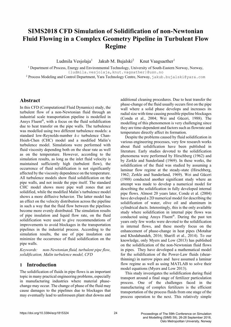
The particular fluid used in this study is a shear-thinning

slurry whose viscosity depends on both the shear rate

and the temperature. The rheological properties of the

fluid taken into consideration were obtained

experimentally using Anton Paar Modular Compact

Rheometer 302. The experimentally obtained flow

curve was fitted to different rheological models. The

best fit was obtained with the Power-Law model for

non-Newtonian fluids. The fitted flow curve used in this

study is illustrated in Figure 1.

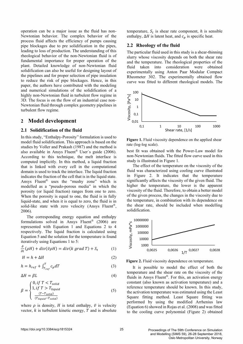
The effect of the temperature on the viscosity of the

fluid was characterized using cooling curve illustrated

in Figure 2. It indicates that the temperature

significantly affects the viscosity of the given fluid. The

higher the temperature, the lower is the apparent

viscosity of the fluid. Therefore, to obtain a better model

of the given process, the changes in the viscosity due to

the temperature, in combination with its dependence on

the shear rate, should be included when modelling

solidification.

It is possible to model the effect of both the

temperature and the shear rate on the viscosity of the

fluids in Ansys Fluent®. For this, an activation energy

constant (also known as activation temperature) and a

reference temperature should be known. In this study,

the activation temperature was estimated using the Least

Square fitting method. Least Square fitting was

performed by using the modified Arrhenius law

(Equation 6) showed in Rojas et al. (2008) and was fitted

to the cooling curve polynomial (Figure 2) obtained

0,01

0,1

1

10

100

0,1 1 10 100 1000V

isco

sity

, [P

a*s]

Shear rate, [1/s]

Figure 1. Fluid viscosity dependence on the applied shear

rate (log-log scale).

1000

10000

100000

1000000

10000000

0,0025 0,0026 0,0027 0,0028

Vis

cosi

ty, m

Pa*

s

1/T

Figure 2. Fluid viscosity dependence on temperature.



experimentally. The estimated value of the activation

temperature (𝛼) is listed in Table 2.

𝜇 = 𝜇∞ exp (𝐸

𝑅𝑇) (6)

where 𝜇 is apparent viscosity, 𝜇∞ is infinite viscosity, 𝐸

is energy, and 𝑅 is universal gas constant.

2.3 Turbulence model

The standard k-ε turbulence model is widely used in

modelling of internal turbulent pipe flows due to its

simplicity and applicability. However, the standard k-ε

turbulence model does not account for drag reduction

effect and may have unsatisfactory results and

predictions at the near wall zones where eddy viscosity

changes rapidly with the distance from the pipe wall

(Mathur and He, 2013; Versteeg and Malalasekera,

2007). This might have a crucial role in modelling

solidification since the solidification of the fluid is

expected to occur on pipe walls. One solution to

overcome this problem is to use low-Reynolds-number

k-ε turbulence models that are specifically developed to

account for near-wall phenomena. However, the fluid

taken into consideration exhibits a highly non-

Newtonian behaviour. To account for this phenomena,

in this paper Malin’s turbulence model for Power-Law

fluids has been modified (Vesjolaja, 2016).

Malin (Malin, 1997; Malin, 1998) has developed a

model where the damping functions are specially treated

to describe the non-Newtonian fluid flow in the

turbulent flow regime (Reynolds number (Re) up to

105). Malin’s model is based on low-Reynolds-number

k-ε turbulence models like the Lam-Bremhost (LB)

model (Lam and Bremhost, 1981). The only and the

most important difference between these two models is

in the way the eddy/turbulent viscosity is calculated. For

both models, the transport equation for the kinetic

energy is formulated as in the standard k-ε turbulence

models and can be founded in earlier works (Malin,

1997; Lam and Bremhost, 1981). However, the eddy

dissipation rate formulation that carries turbulent

viscosity term differs between the two models. With the

Malin’s turbulence model, the formulation of eddy

viscosity includes the power-law index (that carries the

non-Newtonian characteristics) in the damping function

term, while this is not present in the Lam-Bremhost

model.

The transport equation for the eddy dissipation rate

is given by Equation 7, meanwhile the turbulent

viscosity is calculated by Equation 8 using damping

functions (𝑓1, 𝑓2 and 𝑓𝜇) defined in Table 1 (Malin,

1997).

𝜕(𝜌𝜀)

𝜕𝑡+ 𝑑𝑖𝑣(𝜌𝜀𝑈) = 𝑑𝑖𝑣 (

𝜇𝑡

𝜎𝜀𝑔𝑟𝑎𝑑 𝜀) +

𝑓1𝐶1𝜀

𝑘2𝜇𝑡𝑆. 𝑆 − 𝑓2𝐶2𝜌

𝜀2

𝑘 (7)

𝜇𝑡 = 𝐶𝜇𝑓𝜇𝑘2/𝜀 (8)

where 𝜀 is turbulent dissipation rate, 𝑈 is velocity

component, 𝜇𝑡 is turbulent viscosity, and 𝐶1, 𝐶2 and 𝐶𝜇

are turbulence adjustable constants.

Malin’s turbulence model is not readily available in

Ansys Fluent®. It is possible to implement Malin’s

turbulent model by using User Defined Functions

(UDF), however the computational time for the

convergence of the solution is prolonged significantly.

The increased computational time is even more

pronounced when modelling thermal effects

(solidification in this case). Hence, the Malin’s

turbulence model was implemented in a robust way by

enabling and modifying the built-in low-Reynolds-

number k-ε model. For this, Malin’s eddy viscosity

formulation was coupled to the built-in CHC (Chang et

al., 1995) turbulence model using a UDF. The CHC

model was preferred to the LB model as well to other

turbulence models available in Ansys Fluent® e.g.

Launder-Sharma, Abid, Yang-Shih and the Abe-

Kondoh-Nagano models. This choice is based on the

fact, also supported by previous studies (Vesjolaja,

2016) that the CHC model exhibits more stable

solutions during the simulations. Both the standard CHC

and the modified Malin’s models were compared in this

study (see Equations 7, 8 and Table 1 for the algebraic

equations used in different models).

Turbulence Model 𝑓1 𝑓2 𝑓µ Wall

boundary

conditions

Malin original

(Malin, 1997) 1 + (

0.05

𝑓𝜇)3

1 − exp(−Ret2) (1 − exp(−0.0165Rek/n1/4))2 ∗

(1 + 20.5/Ret)

𝜕𝜀

𝜕𝑦= 0

CHC original

(Chang et al.,

1995)

1.0 (1 − 0.01 exp(−Ret2))

∗ (1 − exp (−0.0631Rek)) (1 − exp(−0.0215Rek))2 ∗ (1 +

31.66/𝑅𝑒𝑡5/4

) 𝜀𝑤 = 𝜈(

𝜕2𝑘

𝜕𝑦2)

Modified Malin’s

(Vesjolaja, 2016) 1.0 (1 − 0.01 exp(−Ret

2)) ∗ (1− exp (−0.0631Rek))

(1 − exp(−0.0165Rek/n1/4))2 ∗

(1 + 20.5/Ret) 𝜀𝑤 = 𝜈(

𝜕2𝑘

𝜕𝑦2)

Table 1. Turbulence model damping functions used in Equations 7 and 8.



3 Fertilizer process as a case study

A case study has been performed where the modified

Malin’s model and the CHC model described in Section

2.2 is used to simulate the flow of a non-Newtonian fluid

in 3D. The case study consists of the flow through a

bended pipeline as shown in Figure 3. Geometry of the

pipelines for the process taken into consideration.Figure

3 and is a part of a process from a fertilizer production

plant.

Figure 3. Geometry of the pipelines for the process taken

into consideration.

The pipework consists of the main pipeline which has

a bend of 90° and two additional pipelines (denoted as

“Transportation line 1” and “Transportation line 2” in

Figure 3) that are attached right after the main pipeline

bend. The diameter of the main pipeline is 150 mm and

that of the two transportation lines is 75 mm each. The

thickness of the pipe walls is 5 mm and the pipe material

is stainless steel. The characteristics of the pipe wall

material are listed in Table 2.

The process fluid is pumped through the main

pipeline inlet (denoted as “Inlet” in Figure 3) and is

transported to the next stage of operation through the

Transportation lines 1 and 2. The remaining process

fluid is recirculated using the “Recirculation” line as

denoted in Figure 3.

During the operation of the fertilizer plant, reduced

pump capacity at the inlet of the pipe was observed. It is

suspected that this could be due to the solidification of

the fluid in the pipelines. This study thus focuses on

understanding as to where and how such solidification

occurs in the pipelines. For this, a suitable model

capable of taking into account the rheology of the non-

Newtonian fluid is simulated in Ansys Fluent®. Detailed

3D simulations have been performed to observe where

and how such solidification occurs for a given operating

condition of the process giving a result for steady state

under the selected boundary conditions.

4 Methods and materials

General settings: The simulation of the given process

were performed using commercial CFD tool, Ansys

Fluent® Academic Research, Release 16.2. The

geometry was designed using Ansys DesignModeler

and mesh was generated using sweep mesh method with

the element size of 5 mm and 10° curvatures (1681179

cells in the simulation domain). The simulations were

performed for the 3D steady-state regime using pressure

based solver and absolute velocity formulation.

Momentum Boundary Conditions: The inlet

velocities were varied from 3.0 m/s to 5.0 m/s in

accordance to the different simulation case studies. The

inlet velocities were defined to be the same over the

whole cross sectional area of the pipe inlet. The pipeline

outflows were defined as pressure outlets and gauge

pressure was set to zero.

The estimation of the Reynolds-number for the

internal pipe flow under consideration is challenging

due to the non-Newtonian behavior of the fluid. In this

study, the “generalized Reynolds-number” has been

calculated using the Dodge and Metzner correlation

(Dodge and Metzner, 1959) for the Power-Law fluids

(Equation 9). For the calculation of the Reynolds-

number, the inlet velocity (𝑣𝑏𝑢𝑙𝑘) was taken as a bulk

velocity.

𝑅𝑒 =(𝜌∗𝑣𝑏𝑢𝑙𝑘

2−𝑛 ∗𝐷𝑛)

𝐾(0.75+0.25

𝑛)𝑛∗8𝑛−1

(9)

where 𝐷 is diameter of the pipe, 𝑛 is non-Newtonian

index, 𝐾 is consistency index.

Turbulence model: Turbulent flow was modelled

using the standard CHC turbulence model and the

modified Malin’s model as described in Section 2.3. The

modified Malin’s turbulence model was implemented

using UDF.

Thermal Boundary Conditions: The inlet fluid

temperature as well as the temperature for the backflow

Material ρ (kg/m3)

𝐶𝑝

(J/(kg∙K))

kth (W/(m∙K))

Tliq (K)

Tsol (K)

Tref (K)

α (K)

Fluid 1400 1470 0.3 403 393 303 18100

Pipe Wall

(stainless steel)

Wall insulation

(calcium silicate)

7900

210

515

840

16.6

0.08

Not used

Not used

Not used

Not used

Not used

Not used

Not used

Not used

Table 2. Thermo-physical properties of the materials used in this study.



of the fluid at the outlets was set to 413 K. The wall heat

transfer was modelled using “Thin Wall approach” and

the wall temperature was set to 296 K.

Solution methods: The simulations were performed

in a steady-state regime. The Semi-Implicit Method for

Pressure Linked Equations (SIMPLE) method was used

as a pressure-velocity coupling scheme. The first order

upwind scheme was chosen as a spatial discretization

method. The standard solution initialization was used

for the standard CHC turbulence model. However, when

simulating with the modified Malin’s turbulence model,

the solution was initialized with the end results of the

corresponding CHC model (simulated with the standard

settings). The mesh sensitivity study was performed and

the solution was assumed to be converged when the

scaled residuals become constant. In addition, mass

flowrates were checked and the solution was assumed to

be converged if the mass flowrate imbalance was less

than 10-4. Mass outflow rates were computed using

Surface Integrals available in Ansys Fluent®.

Material properties: The non-Newtonian behavior

of the fluid was characterized with the Power-Law

model for non-Newtonian fluids (𝑛 = 0.05). The thermo-

physical properties of the fluid and the wall material

(including wall insulation) used for simulations are

summarized in Table 2.

5 Results and Discussion

5.1 Effect of temperature on fluid’s viscosity

To have a better understanding of how the temperature

affects the viscosity of the non-Newtonian fluid and how

this further influences the fluid solidification,

simulations were modelled using standard CHC

turbulence model. To start with, the fluid flow rate

corresponding to the transient flow regime (with Re =

6796 and the inlet velocity of 3.0 m/s) was considered.

Two cases were studied: (a) viscosity dependent only on

the shear rate and, (b) viscosity dependent on both the

temperature and the shear rate, and results are shown in

Figure 4.

Figure 4. Solidification profiles using CHC model with 3

m/s inlet velocity for fluid with: (a) shear rate dependent

viscosity; (b) both shear rate and temperature dependent

viscosity.

Both simulations showed fluid solidification on the

pipe walls, meanwhile no solidification occurred inside

the pipe itself for both cases. Moreover, at the pipe

walls, observable differences in the solidification

profiles were seen for the two cases. For the first case

(viscosity not affected by temperature), smaller

solidification zones were observed (Figure 4a)

compared to the results obtained for the latter case (see

Figure 4b).

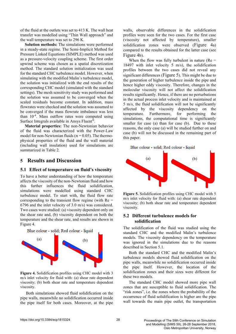
When the flow was fully turbulent in nature (Re =

18497 with inlet velocity 5 m/s), the solidification

profiles between the two cases did not reveal any

significant differences (Figure 5). This might be due to

the generation of higher turbulence inside the pipe and

hence higher eddy viscosity. Therefore, changes in the

molecular viscosity will not affect the solidification

results significantly. Hence, if there are no perturbations

in the actual process inlet velocity and is maintained at

5 m/s, the fluid solidification will not be significantly

affected by the viscosity dependency on the

temperature. Furthermore, for performing the

simulations, the computational time is significantly

smaller for case (a) than for case (b). Due to these

reasons, the only case (a) will be studied further on and

case (b) will not be discussed in the remaining part of

this paper.

Figure 5. Solidification profiles using CHC model with 5

m/s inlet velocity for fluid with: (a) shear rate dependent

viscosity; (b) both shear rate and temperature dependent

viscosity.

5.2 Different turbulence models for

solidification

The solidification of the fluid was studied using the

standard CHC and the modified Malin’s turbulence

models. The viscosity dependency on the temperature

was ignored in the simulations due to the reasons

described in Section 5.1.

Both the standard CHC and the modified Malin’s

turbulence models showed fluid solidification on the

pipe walls, meanwhile no solidification occurred inside

the pipe itself. However, the location of the

solidification zones and their sizes were different for

these two models.

The standard CHC model showed more pipe wall

zones that are susceptible to fluid solidification. The

“risk zones”, i.e. the zones where the probability of the

occurrence of fluid solidification is higher are the pipe

wall towards the main pipe outlet, the transportation

(a) (b)

(a) (b)



pipeline walls and the backside of the pipe wall just

before the main pipe bend (denoted as “zone 1”, “zone

2” and “zone 3” respectively in Figure 6). The

occurrence of the fluid solidification on “zone 1” can be

explained with the presence of a larger surface area of

the wall that is exposed to the ambient air temperature.

The larger the surface area, the larger will be the heat

transfer between the ambient air and the fluid and hence

more fluid will be solidified. Solidifications on “zone 2”

and “zone 3” can be explained with the occurrence of

lower fluid velocities at these zones. The lower the

velocity, the slower the fluid molecules are moving

inside the pipe and hence these molecules have

comparatively more time to exchange heat with the

ambient air through the pipe walls.

The modified Malin’s turbulence model showed

different and smaller “risk zones” for solidification

compared to the CHC model. The solidification of the

fluid occurred after the main pipe bend and near the

outlet of the transportation Pipelines 1 and 2 (denoted as

“zone 4” and “zone 5” respectively in Figure 7). From

the velocity profiles it can be seen that these zones are

the low-velocity zones or the “dead zones”.

The occurrence of solidification on these zones can

also be explained with a longer residence time of the

fluid molecules (due to lower velocity) in these zones

and hence more transfer of heat from the fluid to the

ambient air through the pipe walls. Interestingly in

contrast to the standard CHC model, the modified

Malin’s model can capture these “dead zones” which are

the “risk zones” for fluid solidification. The occurrence

of less solidification along the pipeline walls can be

explained with the diffusive behaviour of the modified

Malin’s model (see velocity profiles on Figure 6a and

Figure 7a). The higher the turbulence, the higher is the

velocity and hence the less is the residence time of the

fluid molecule inside the pipeline. Therefore, this causes

fewer fluid molecules to solidify on the pipe walls. The

modified Malin’s model shows more evenly distributed

mass outflow rates and hence evenly distributed

velocities along the pipelines.

5.3 Effect of pipe wall insulation on

solidification

To investigate if the insulation of the pipelines would

minimize the occurrence of fluid solidification, the

simulations were also performed with the changes in the

thickness of the pipe wall insulation. The properties of

the insulation layer are summarized in Table 2. The

solidification was simulated using both the standard

CHC and the modified Malin’s turbulence models.

Both turbulence models showed similar simulation

results revealing that no solidification occurred when

the pipe wall was insulated with a 50 mm-thick

insulation layer jacket. This behavior was observed for

the higher fluid velocity (5 m/s) as well as for the lower

fluid velocity (3 m/s). However, without pipe insulation,

the fluid solidifies at different places along the pipeline

Figure 7. Simulation results with the modified Malin’s model (3 m/s inlet velocity): (a) velocity profile; (b) fluid

solidification.

Figure 6. Simulation results with the CHC model (3 m/s inlet velocity): (a) velocity profile; (b) fluid solidification.

(b)

(b) (a)

(a)



as described in the previous sections. Thus, the absence

of the pipe wall insulation could be a probable reason

for the detected reduced pump capacity during the

operation process.

6 Conclusions

The solidification model was coupled to the non-

Newtonian turbulence model in Ansys Fluent® by using

UDFs. The “Enthalpy-Porosity” formulation was used

to model fluid solidification, meanwhile modified

Malin’s model was used to model turbulent fluid flow.

The Malin’s eddy viscosity model was combined with

the low-Reynolds-number k-ε turbulence Chan-Hsieh-

Chen model to account for the non-Newtonian

behaviour of the process fluid.

As long as the inlet fluid velocity is maintained

sufficiently high (turbulent flow), the occurrence of

fluid solidification is not significantly affected by the

viscosity dependence on the temperature. According to

the simulation results, both the CHC and modified

Malin’s turbulence models showed fluid solidification

on the pipe walls, and not inside the pipe itself. The

location and the size of fluid solidification zones were

different for these two models. Modified Malin’s model

showed more diffusive behaviour. It is difficult to

conclude which of these models better represents the

real process. Validation of the simulation results should

be considered as a potential future work.

According to the simulation results, the use of pipe

insulation can minimize the occurrence of fluid

solidification on the pipe walls. Without insulation,

solidification occurred on the pipe walls. Thus, the use

of pipe insulation is beneficial and is highly

recommended for the investigated process.

Acknowledgements

Authors kindly thank the department of Process

Modelling and Control at Yara International ASA for

providing the knowledge about the process. We would

also like to thank the NPK department at Yara specially

Carole Allen for her contributions in performing

experiments.

References

Chang, K., Hsieh, W., & Chen, C. (1995). A modified low-

Reynolds-number turbulence model applicable to

recirculating flow in pipe expansion. Journal of fluids

engineering, 117(3), 417-423.

Conde, R., Parra, M., Castro, F., Villafruela, J., Rodrıguez,

M., & Méndez, C. (2004). Numerical model for two-phase

solidification problem in a pipe. Applied Thermal

Engineering, 24(17), 2501-2509.

Dodge, D., & Metzner, A. (1959). Turbulent flow of non‐

Newtonian systems. AIChE Journal, 5(2), 189-204.

Ansys Fluent® 6.3 User's Guide, (2006).

Hirschberg, H. (1962). Freezing of piping systems.

Kaltetechnik, 14, 314-321.

Lam, C., & Bremhost, K. (1981). A modified form of the k-ε

model for predicting wall turbulence. ASME J. Fluids Eng,

103, 456-460.

Malin, M. (1997). Turbulent pipe flow of power-law fluids.

International communications in heat and mass transfer,

24(7), 977-988.

Malin, M. (1998). Turbulent pipe flow of Herschel-Bulkley

fluids. International communications in heat and mass

transfer, 25(3), 321-330.

Mathur, A., & He, S. (2013). Performance and

implementation of the Launder–Sharma low-Reynolds

number turbulence model. Computers & Fluids, 79, 134-

139.

Motahar, S., & Khodabandeh, R. (2016). Experimental study

on the melting and solidification of a phase change material

enhanced by heat pipe. International communications in

heat and mass transfer, 73, 1-6.

Myers, T., & Low, J. (2013). Modelling the solidification of a

power-law fluid flowing through a narrow pipe.

International Journal of Thermal Sciences, 70, 127-131.

Rojas, M. A., Castagna, J., Krishnamoorti, R., & Han Dh, T.

A. (2008). Shear thinning behavior of heavy oil samples:

laboratory measurements and modeling. Paper presented at

the SEG Annual Meeting, Las Vegas.

Sharifi, N., Bergman, T. L., Allen, M. J., & Faghri, A. (2014).

Melting and solidification enhancement using a combined

heat pipe, foil approach. International Journal of Heat and

Mass Transfer, 78, 930-941.

Versteeg, H. K., & Malalasekera, W. (2007). An introduction

to computational fluid dynamics: the finite volume method:

Pearson Education.

Vesjolaja, L. (2016). Flow Patterns of Highly Non-Newtonian

Fluids in Industrial Applications. Master Thesis in Process

Technology, Department of Process, Energy and

Environmental Technology, University College of

Southeast Norway.

Voller, V. R., & Prakash, C. (1987). A fixed grid numerical

modelling methodology for convection-diffusion mushy

region phase-change problems. International Journal of

Heat and Mass Transfer, 30(8), 1709-1719.

Wei, S.-S., & Güceri, S. I. (1988). Solidification in developing

pipe flows. International Journal of Heat and Fluid Flow,

9(2), 225-232.

Zerkle, R. D., & Sunderland, J. (1968). The effect of liquid

solidification in a tube upon laminar-flow heat transfer and

pressure drop. Journal of Heat Transfer, 90(2), 183-189.



Documents

SIMS2018 CFD Simulation of Solidification of non-Newtonian