Embed Size (px)
Citation preview

Simplified Adaptive Control ofCentrifugal Compressors
Andrzej Tomasz Jerzak
Master of Science in Cybernetics and Robotics
Supervisor: Jan Tommy Gravdahl, ITK
Department of Engineering Cybernetics
Submission date: January 2017
Norwegian University of Science and Technology


SummaryIn this thesis adaptive surge control in axial and centrifugal compressor with unknowncharacteristic was studied. The compressor to be viewed as the control target, was a partof the compression system which also included the plenum and a throttling device, bothlocated downstream to the compressor.
The literature offers already several research papers dealing with adaptive control of com-pressors, where the knowledge of the compressor map is not needed in advance. Sum-maries of some of the papers has been offered in this thesis. The author proposed a sim-plified version of an adaptive controller where the controller gain is being calculated byestimating the compressor characteristic. The estimation was carried out by using the mostbasic identification techniques: method of steepest decent and the least-squares.
Both strategies estimated the unknown coefficients of the compressor characteristic by pro-cessing input/output data of the latter on-line. The input signal for the estimation schemeconsisted of a flow measurement at the compressor duct while the pressure rise at thecompressor would constitute the output signal. Occasionally, the flow at the compressorduct will be unavailable for measurement. As a solution, the compression system will wascoupled with an observer which predicted the behaviour of the compressor duct flow byconsidering the model for entire compression system. The observer originated from [12]where it has been proven that the flow is being predicted in a exponentially stable manner.The core of each of the estimation methods was the adaptive law, which will continuouslyupdates the estimates of the unknown coefficients. The trajectories of the estimates wasall said to be bounded functions. Strictly speaking, they are considered as elements of L∞and L2 spaces. This was verified with stability analysis where Lyapunov’s direct methodwas applied. The stability analysis was previously published in [33] and has were includedin this report.
Two types of actuators for surge control were considered: closed-coupled valve (CCV)and a piston. The resulting control law for both actuators was a basic proportional con-troller which recovered the compression system from surge and bring it towards globalasymptotic stability. The controller operating CCV required feedback from compressormass flow measurement while the piston was being run by the controller that requiredfeedback from pressure measurements at the compressor discharge and at the plenum. Byassigning the actuator and the controllers, the compressor was brought to global asymp-totic stability even if it was operating at the unstable area in the first place. In the past, thegain for each controller was constructed by the coefficients used to describe the compres-sor characteristic. In subject to not knowing the compressor characteristic, the coefficientsappearing in the controller would be replaced by their estimates which were generated bythe earlier mentioned adaptive laws. The implementation of the adaptive laws dependedon the knowledge of the coordinates of the system equilibrium. Yet another adaptive lawwas implemented to estimate the coordinates. The estimation was needed for equilibrium, since the computation of the latter is restricted to knowing the compressor characteristic.Linearization of the compression system augmented with the adaptive controller and theequilibrium estimation was used as a tool to demonstrate that under specific conditions theoverall systems becomes locally asymptotically stable.
i

Preface
This thesis is submitted in partial fulfillment of the requirements for the master’s degree inEngineering Cybernetics at the Norwegian University of Science and Technology.The work on the thesis spanned from September 2016 to January 2017.
First of all, I would like to thank my supervisor Professor Jan Tommy Gravdahl. Thisthesis would never take place without his involvement. Not only did he let me work onthe field of adaptive control of compressors, but throughout the period of the thesis, he hasanswered my questions of different issues.
I am also grateful to Nur Uddin, a PhD graduate from Department of Engineering Cyber-netics at NTNU, for willingly sharing his knowledge on piston actuation.
My best regards and acknowledgements goes to Tor Wilhelm Seim, chief executive officerat Albaran AS, for providing a working place for me and for his effort of creating a warmand inclusive atmosphere so that I could fully concentrate on my thesis.
Finally, I would like to express my love to my brother Alexander and to my parents, HaraldDamhaug and Ewa Jerzak-Damhaug.
Andrzej JerzakJanuary 2017
ii

Table of Contents
Summary i
Preface ii
Table of Contents iv
List of Tables v
List of Figures vii
Abbreviations viii
1 Introduction and Motivation 11.1 Background . . . . . . . . . . . . . . . . . . . . . . . . . . . . . . . . . 11.2 Centrifugal Compressors . . . . . . . . . . . . . . . . . . . . . . . . . . 31.3 Compressor Map . . . . . . . . . . . . . . . . . . . . . . . . . . . . . . 41.4 Compressor Instability . . . . . . . . . . . . . . . . . . . . . . . . . . . 7
1.4.1 Rotating Stall . . . . . . . . . . . . . . . . . . . . . . . . . . . . 71.4.2 Surge . . . . . . . . . . . . . . . . . . . . . . . . . . . . . . . . 8
1.5 Contributions . . . . . . . . . . . . . . . . . . . . . . . . . . . . . . . . 91.6 Implementation . . . . . . . . . . . . . . . . . . . . . . . . . . . . . . . 101.7 Outline of the Thesis . . . . . . . . . . . . . . . . . . . . . . . . . . . . 10
2 The Model of Greitzer 122.1 Introduction . . . . . . . . . . . . . . . . . . . . . . . . . . . . . . . . . 122.2 Description of the Greitzer Model . . . . . . . . . . . . . . . . . . . . . 122.3 Derivation of the Dynamic Equations for the Greitzer Model . . . . . . . 142.4 Non-dimensionalization of the Greitzer model . . . . . . . . . . . . . . . 152.5 Equilibrium Point and Open-Loop Stability . . . . . . . . . . . . . . . . 17
3 Surge Control 203.1 Introduction . . . . . . . . . . . . . . . . . . . . . . . . . . . . . . . . . 203.2 Surge Avoidance System (SAS) . . . . . . . . . . . . . . . . . . . . . . 213.3 Active Surge/Stall Control System (ASCS) . . . . . . . . . . . . . . . . 22
iii

3.3.1 Closed-Couple Valve . . . . . . . . . . . . . . . . . . . . . . . . 233.3.2 Piston Actuation . . . . . . . . . . . . . . . . . . . . . . . . . . 25
3.4 Determination of the Equilibrium Point . . . . . . . . . . . . . . . . . . 28
4 On-Line Parameter Estimation 324.1 Introduction and Definition . . . . . . . . . . . . . . . . . . . . . . . . . 324.2 Mathematical preliminaries . . . . . . . . . . . . . . . . . . . . . . . . . 33
4.2.1 Lp Spaces . . . . . . . . . . . . . . . . . . . . . . . . . . . . . . 334.2.2 Lp Stability . . . . . . . . . . . . . . . . . . . . . . . . . . . . . 33
4.3 Linear Parametric Model . . . . . . . . . . . . . . . . . . . . . . . . . . 344.4 Method of Steepest Descent . . . . . . . . . . . . . . . . . . . . . . . . 354.5 Method of Least-Squares . . . . . . . . . . . . . . . . . . . . . . . . . . 38
5 Observer for Inlet Flow 425.1 Introduction . . . . . . . . . . . . . . . . . . . . . . . . . . . . . . . . . 425.2 GES flow observer . . . . . . . . . . . . . . . . . . . . . . . . . . . . . 435.3 Non-dimentionalization of the observer equations . . . . . . . . . . . . . 445.4 A Separation Principle . . . . . . . . . . . . . . . . . . . . . . . . . . . 46
6 Adaptive Compressor Control in the Literature 486.1 Adaptive Extension of Active Surge Control Using Drive Torque . . . . . 486.2 High-Gain Type Adaptive Control For Surge Stabilization . . . . . . . . . 506.3 Adaptive Fuzzy Control of Compressor Surge . . . . . . . . . . . . . . . 54
7 Simulation 617.1 Preliminaries . . . . . . . . . . . . . . . . . . . . . . . . . . . . . . . . 617.2 System specifications . . . . . . . . . . . . . . . . . . . . . . . . . . . . 627.3 Open-loop simulation . . . . . . . . . . . . . . . . . . . . . . . . . . . . 62
7.3.1 Stable operation . . . . . . . . . . . . . . . . . . . . . . . . . . 627.3.2 Surge Condition . . . . . . . . . . . . . . . . . . . . . . . . . . 63
7.4 Closed-loop simulation . . . . . . . . . . . . . . . . . . . . . . . . . . . 647.4.1 Calculations of the compressor characteristic coefficients . . . . . 647.4.2 Simulations of the single compression system with CCV as the
actuator . . . . . . . . . . . . . . . . . . . . . . . . . . . . . . . 657.4.3 Simulations of PAASCS . . . . . . . . . . . . . . . . . . . . . . 74
8 Discussion 84
9 Conclussion 86
iv

List of Tables
7.1 Specifications for the compression system . . . . . . . . . . . . . . . . . 62
v

List of Figures
1.1 Positive displacement pump operation . . . . . . . . . . . . . . . . . . . 21.2 The components making up the centrifugal compressor . . . . . . . . . . 31.3 Compressor map . . . . . . . . . . . . . . . . . . . . . . . . . . . . . . 51.4 Compressor map obtained by the performance test . . . . . . . . . . . . . 61.5 Physical mechanism for inception of rotating stall . . . . . . . . . . . . . 71.6 Surge cycle illustrated in a compressor map . . . . . . . . . . . . . . . . 8
2.1 Model of a single compression system . . . . . . . . . . . . . . . . . . . 132.2 Compressor and throttle characteristic in the same coordinate system . . . 17
3.1 Trajectory of the compressor system prevented from going into surge . . . 213.2 Single compression system extended with CCV . . . . . . . . . . . . . . 243.3 Compression system equipped with piston . . . . . . . . . . . . . . . . . 26
6.1 Results of high-gain anti-surge adaptive control . . . . . . . . . . . . . . 546.2 A membership function for a positive and large real number . . . . . . . 566.3 The block diagram of the whole adaptive controller . . . . . . . . . . . . 586.4 Simulation results . . . . . . . . . . . . . . . . . . . . . . . . . . . . . . 596.5 Controller output . . . . . . . . . . . . . . . . . . . . . . . . . . . . . . 60
7.1 Inlet flow for stable operation expressed with a dimensionless standardvariable . . . . . . . . . . . . . . . . . . . . . . . . . . . . . . . . . . . 63
7.2 Plenum pressure for stable operation . . . . . . . . . . . . . . . . . . . . 637.3 Inlet flow during surge expressed with a dimensionless standard variable [] 647.4 Plenum pressure during surge expressed with a dimensionless standard
variable . . . . . . . . . . . . . . . . . . . . . . . . . . . . . . . . . . . 647.5 Stabilization of the inlet flow with both the standard P-controller and the
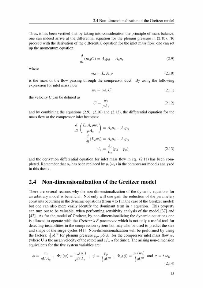
adaptive controller . . . . . . . . . . . . . . . . . . . . . . . . . . . . . 667.6 Comparing inlet flow measurement with its estimate . . . . . . . . . . . . 677.7 Stabilization of the plenum pressure with both the standard P-controller
and the adaptive controller . . . . . . . . . . . . . . . . . . . . . . . . . 677.8 Trajectory of the estimate for k1 . . . . . . . . . . . . . . . . . . . . . . 687.9 Trajectory of the estimate for k2 . . . . . . . . . . . . . . . . . . . . . . 68
vi

7.10 Trajectory of the estimate for k3 . . . . . . . . . . . . . . . . . . . . . . 697.11 Trajectory of the estimate for φ0 . . . . . . . . . . . . . . . . . . . . . . 697.12 Trajectory of the estimate for ψ0 . . . . . . . . . . . . . . . . . . . . . . 707.13 Stabilization of the inlet flow with both the standard P-controller and the
adaptive controller . . . . . . . . . . . . . . . . . . . . . . . . . . . . . 717.14 Comparing inlet flow measurement with its estimate . . . . . . . . . . . . 717.15 Stabilization of the plenum pressure with both the standard P-controller
and the adaptive controller . . . . . . . . . . . . . . . . . . . . . . . . . 727.16 Trajectory of the estimate for k1 . . . . . . . . . . . . . . . . . . . . . . 727.17 Trajectory of the estimate for k2 . . . . . . . . . . . . . . . . . . . . . . 737.18 Trajectory of the estimate for k3 . . . . . . . . . . . . . . . . . . . . . . 737.19 Trajectory of the estimate for φ0 . . . . . . . . . . . . . . . . . . . . . . 747.20 Trajectory of the estimate for ψ0 . . . . . . . . . . . . . . . . . . . . . . 747.21 Stabilization of the inlet flow with both the standard P-controller and the
adaptive controller . . . . . . . . . . . . . . . . . . . . . . . . . . . . . 767.22 Comparing inlet flow measurement with its estimate . . . . . . . . . . . . 767.23 Stabilization of the plenum pressure with both the standard P-controller
and the adaptive controller . . . . . . . . . . . . . . . . . . . . . . . . . 777.24 Trajectory of the estimate for k1 . . . . . . . . . . . . . . . . . . . . . . 777.25 Trajectory of the estimate for k2 . . . . . . . . . . . . . . . . . . . . . . 787.26 Trajectory of the estimate for k3 . . . . . . . . . . . . . . . . . . . . . . 787.27 Trajectory of the estimate for φ0 . . . . . . . . . . . . . . . . . . . . . . 797.28 Trajectory of the estimate for ψ0 . . . . . . . . . . . . . . . . . . . . . . 797.29 Stabilization of the inlet flow with both the standard P-controller and the
adaptive controller . . . . . . . . . . . . . . . . . . . . . . . . . . . . . 807.30 Comparing inlet flow measurement with its estimate . . . . . . . . . . . . 807.31 Stabilization of the plenum pressure with both the standard P-controller
and the adaptive controller . . . . . . . . . . . . . . . . . . . . . . . . . 817.32 Trajectory of the estimate for k1 . . . . . . . . . . . . . . . . . . . . . . 817.33 Trajectory of the estimate for k2 . . . . . . . . . . . . . . . . . . . . . . 827.34 Trajectory of the estimate for k3 . . . . . . . . . . . . . . . . . . . . . . 827.35 Trajectory of the estimate for φ0 . . . . . . . . . . . . . . . . . . . . . . 837.36 Trajectory of the estimate for ψ0 . . . . . . . . . . . . . . . . . . . . . . 83
vii

Abbreviations
MPC = Model Predictive Control
LQR = Linear Quadratic Regulator
SAS = Surge Avoidance System
ASCS = Active Surge Control System
SL = Surge Line
SCL = Surge Control Line
SM = Surge Margin
CCV = Closed-Coupled Valve
PAASC = Piston Actuated Active Surge Control
LMI = Linear Matrix Inequality
SPR = Strictly Positive Real
viii

Chapter 1Introduction and Motivation
1.1 BackgroundThe compressor can be viewed as a mechanic device that has the potential of increasingthe pressure of the fluid passing through it. A way of achieving such pressure rise is bybasically decreasing the fluids volume. The bellow ideal gas law can be studied as anexplanation to this phenomena:
p =mRT
V(1.1)
where R is the gas constant. Moreover, p is the pressure of the fluid, while m, T and Vare its mass,temperature and volume. respectively. A point made by [10] is that due to thedefinition of density being ρ = m
V , the compressor can alternatively be viewed as a devicethat provides gain in fluid pressure by increasing the density of the fluid. Over the years,the compressors has been used in a wide range of applications [34]. They are essential ingas turbines for power generation (Brayton cycle) and jet engines in aircraft. One can alsofound them in many household appliances such as refrigerators and air conditioners. Inaddition the compressors are commonly applied in process industry, where they are usedto transport fluids through pipelines, for example in chemical plants and/or oil and naturalgas production installations.
There are various types of compressors, some of them being centrifugal compressors, axialcompressors and the positive displacement pumps. The axial and centrifugal compressors(termed turbo compressors by [10]) works by somewhat equal principle of operation whichmainly consists of two steps: first increase the velocity of the fluid ,something that is beingdone by running the fluid through a row of rotating blades, and secondly decelerate the gasin divergence channels in order to obtain a pressure rise. The author will follow [10] andexplain the second step by Bernoulli equation:
p1 +1
2ρv2
1 = p2 +1
2v2
2 (1.2)
for the flow assumed to be frictionless incompressible along the pipeline. The subscript”1” refers to the state of the fluid where its velocity is high. Meanwhile, the subscript”2” denotes the state of the fluid where its velocity has been slowed down, i.e. v1 > v2.
1

1.1 Background
Obviously, for the equality in Bernoulli equation to hold, p2 must be greater that p1. Theassumption of incompressibility which will be followed through entire report clearly con-tradicts with the ideal gas law. However, [10] supports this assumption stating that it is”made to illustrate conversion to pressure by means of simple expression”.
The axial compressor got its name from both receiving and discharged the flow in the axialdirection, that is, parallel with the axis of rotation [13]. A compression of a fluid can befurther increased by assigning an axial or centrifugal compressor of multiple stages. Themultiple stages compressors are simply single stages compressors mounted in series andare driven by the same shaft Thus, they are being run by the same rotational speed. Figuresprovided by [13] shows that an industrial single stage axial compressor is able to obtaina pressure rise in order 1.05 : 1 − 1.2 : 1 with the efficiency ranging from 88% to 92%. If several stages are added together, the axial compressors have the potential to obtain apressure rise up to 40 times the original pressure. [13] claims that axial compressor will befrequently encountered in gas turbines, especially for those with power exceeding 5MW.Although research in this thesis is applicable for both axial and centrifugal compressordue to their similarities, this report will emphasize centrifugal compressor, because of itspopularity in the industry. For that reason, a whole subsection will be devoted to discusscentrifugal compressors.
The positive displacement pumps differs significantly from turbo compressors in terms ofworking principle and applications. Instead of accelerating the fluid to a higher velocitylike for turbo compressors, positive displacement pumps obtain a gain in pressure by cap-turing a fixed amount of fluid in a chamber where the volume will be reduced by a pistonmechanism. Once the fluid is compressed to a higher pressure (recall the ideal gas law),the fluid is forced (or displaced) into a discharge pipe or a throttle from which it leavesthe compressor. The principle of operation for the positive displacement pump has beendemonstrated by Figure 1.1
Figure 1.1: Positive displacement pump operation (Marine Notes,http://marinenotes.blogspot.no)
Because of its property of allowing fluid to pass with a low velocity, positive displacementpumps are consequently used in applications where one is requiring a combination of lowflow rate and high pressure, such as pumping media containing fragile solids (ProcessIndustry Forum, http://www.processindustryforum.com/).
2

1.2 Centrifugal Compressors
Finally, positive displacement pumps operate at high efficiency and are the natural choicewhen dealing with high viscosity fluids.
1.2 Centrifugal CompressorsAccording to [14], the centrifugal compressors have three basic components which are theimpeller, the diffuser and the volute (scroll) The impeller can be recognized as a rotatingdisk with curved blades (two-dimentional or three dimensional) and is driven by somedevice (typically a motor or a turbine) which generates a torque τd so that the compressorrotates with angular speed ω. While rotating, the impeller will increase the velocity ofthe incoming fluid and lead it radially outward through the diffuser. From the point ofview of energy domain, one can say that the impeller converts its rotational energy to thekinetic energy in the flow. [48] calls the impeller ”the most critical part of the centrifugalcompressor”, no matter which type of compressor it belongs to. It is further stated that theimpeller stand for 70% of the total pressure rise considering a single stage. If the impelleris well-designed for the compressor, it can reach a efficiency of 96%. Another part of thecompressor, the diffuser, comprises of vane passages and is responsible of slowing downthe fluid and thus generating the pressure rise. The fluid with increased static pressure,is being collected by the volute which guides the fluid to the compressor outlet. Thecompound of the components making up the centrifugal compressor is being shown inFigure 1.2
Figure 1.2: The components making up the centrifugal compressor (ME Mechanical,http://me-mechanicalengineering.com)
3

1.3 Compressor Map
It is primary in the way of discharging the fluid out to the system, that the centrifugalcompressor differs itself from the compressors of axial type. In contrast to axial compres-sors where the fluid is leaving in the axial direction, the fluid departs from the centrifugalcompressor in the direction 90 degrees to the axis of rotating shaft, as proven by Figure1.2. Besides, for the axial compressor, the deceleration of the fluid will take place inthe stator blade passages, instead of the diffuser. The centrifugal compressors are lim-ited to handling much lower flowrates then axial compressors, but in return are capableof delivering much higher pressure ratios. Nevertheless, the units used in the process in-dustry have, according to [15], typically a pressure ratio around 1.3:1 per stage, so onlyslightly higher than for compressors of axial type. On other hand, the centrifugal compres-sors applied in gas turbines range in pressure ratios from 3:1 up to 7:1 for a single stage,clearly overcoming the axial compressors. Evaluation of Figure 7 in [14] shows that axialcompressors beats centrifugal compressor when the overall efficiency is considered. Ac-cording to [14], the centrifugal compressors can typically be found in following servicesof processes : combustion, distribution of natural gas, refrigeration and separation. Theadvantages of centrifugal compressors are that they are compact, robust and less affectedby the performance degradation due to fowling [34]. In his master thesis, [42] states thatthis type of compressors is favoured in the process industry because they are more flexibleand generate lower installation and maintenance costs.
1.3 Compressor MapThe relation between pressure at the compressor inlet, denoted by pi and the pressure atthe compressor outlet, denoted pd is given as follows:
pd = pc(wi, ω)pi (1.3)
where
pc(wi, ω) =
(1 +
µr22ω
2 − r12 (ω − αwi)2 − kfω2
cpT01
) κκ−1
(1.4)
is the pressure rise also to be addressed as the pressure ratio. Throughout the thesis, pdwill be equal to pc. A very important thing to have in mind is that although pc(wi) isnot known as a function, a value of pc at an arbitrary wi is accessible. Notice that thepressure of the compressor rise for the centrifugal compressor depends both on rotationspeed ω[ rads ] at the impeller and the flowwi[
m3
s ] passing through the compressor. The flowwi is termed inlet mass flow (inlet flow when non-dimensionalized). For the definitionsof the constants appearing in eq. (1.4), the reader is referred to [26]. If the compressorrise is to be visualized as a function of inlet mass flow and impeller speed, the compressorcharacteristic (also known as compressor map) will be obtained. The map will often bepresented as the collection of constant speed lines, as shown in Figure 1.3
4

1.3 Compressor Map
Figure 1.3: Compressor map [10]
As the name implies, the constant speed line will relate the pressure ratio to mass flow ata specific rotational speed. A single speed line can also be described by following cubicequation which has been provided by [39]:
pc(wi) = pc0 +H
[1 +
3
2
(wiW− 1)− 1
2
(wiW− 1)3]
(1.5)
where pc0 is the shut-off value of the axisymmetric characteristic, W is semi-width of thecubic axisymmetric compressor characteristic and H is the semi-height of the cubic ax-isymmetric compressor characteristic [51]. A detailed definition of the constant appearingin eq. (1.5) can be found in [39]. The compressor characteristic defines the operationaldomain of the compressor and should always be taken into account when selecting the sizeof the compressor [34]. It is unique for every compressor and will typically be providedby the manufacturer when purchasing the device. Alternatively, it can be retrieved by thecompressor performance test, a procedure described in [52] and which also will be sum-marized later in this section. By analysing Figure 1.3, it can be observed that by eitherreducing the flow rate passing through the compressor (this can be done by adjusting thethrottle opening in the system) or operating the device at higher rotational speed, a greatercompressor rise will be achieved. However, too low flow rate will generate the unwantedphenomena of surge which will drive the compressor to instability. Usually, a surge lineis drawn at the compressor map with the purpose of separating the stable area in the com-pressor map with the area where the surge will develop.
Now, moving to the topic of compressor map test. Simply, it will be performed by firstsetting the compressor to constant speed, then defining several operating points by varyingthe throttle opening and finally recording data of compressor rise and inlet mass flow foreach point. Figure 1.4 shows experimental results of the compressor test done by [52].
5

1.3 Compressor Map
Figure 1.4: Compressor map obtained by the performance test [52]
The impeller was adjusted to a speed of 23978 RPM, and eight operating points wererecorded and labelled sequentially by alphabet A to H. [52] reports that the first sevenoperating points were generated by gradually decreasing the throttle opening from 40%to 10%, resulted in a stable operation of the compressor, with point G approximately lo-cated at the surge line (referred to as the surge point) being the peak of the compressorcharacteristic. Point H, on the other hand, which was obtained by reducing the opening atthe throttle to 5%, is said to be placed at the unstable area, thus bringing surge upon thecompressor.
The cubic function in eq. (1.5) is being modelled by evaluating the instability conditionsbecause of surge, making it valid over the unstable operating area of the compressor char-acteristic (”Approximation 2” in Figure 1.4). According to [52] the value of H is roughlyequal to the amplitude of compressor outlet pressure oscillations (see Figure 4 in [52]),appearing due to the presence of surge. The inlet mass flow recorded for the surge pointis being equal to 2W while the value of pc0 is a result of subtracting 2H from the pressurerise recorded for the surge point. Meanwhile, the compressor characteristic for the stablearea can be approximated by considering operating point A to G. This approach, whichhave been labelled ”Approximation 1” in Figure 1.4, can easily by done with polynomialcurve fitting on the earlier mentioned point. The outcome will be a 3rd order polynomialfunction of inlet mass flow, as depicted in Figure 1.4.
6

1.4 Compressor Instability
1.4 Compressor Instability
1.4.1 Rotating StallCommonly, rotating stall is characterized by disturbance in uniform flow pattern [18]. Incontrast to surge, rotating state will appear locally at the compressor. Strictly speaking, ittends to occur between the blade passages in the impeller (or rotor for axial compressors)where the flow may stall. The region of rotating stall may propagate exponentially alongthe blades until a certain state has been reached [18]. A row of axial compressor bladesoperating at a high angle of attack has been depicted in Figure 1.5.
Figure 1.5: Physical mechanism for inception of rotating stall [23]
[23] describes the propagation mechanism as follows. ”Suppose that there is non-uniformityin the inlet flow such that a locally higher angle of attack is produced on blade B which isenough to stall it. The flow now separates from the suction of the blade, producing a flowblockage between B and C. This blockage causes a diversion of the inlet flow away fromB towards A and C, resulting in a increased angle of attack on C, causing it to stall. Thusthe the stall propagate along the blade row”.
Considering this scenario, the rotating stall can be classified into two types: part-span andfull-span rotating stall. In a part-span rotating stall, only a limited region of the blade pas-sage (the tip in most cases) will stall. For the full-span rotating stall, the stalling will occurat complete heigh of the annulus. Hence, the influence of the rotating stall may also bemeasured by the size of area the flow blockage is taking up in the compressor annulus [23].For the centrifugal compressor, the stalling may be present in the parts of the impeller, inthe diffuser or in the volute. The components may stall simultaneously or individually[18]. However, a stall in one component may not grow sufficiently in strength to spreadto the other areas of the machine. As a consequence, several parts of the centrifugal com-
7

1.4 Compressor Instability
pressor may stall without the entire unit stalling [15]. It turned out that the rotating stallboth in the impeller and the diffuser, may develop into surge for entire system. Neverthe-less, the role of rotating stall in centrifugal compressors is still a matter of debate amongthe compressor researchers. [18] claims that rotating stall often will have little impact onpressure rise for centrifugal compressor and thus on surge. The significance of surge mayalso be questioned for single-stage axial compressors. For multi-stage axial compressors,rotating stall is more relevant for the applications where the shaft speed is relatively low.
1.4.2 SurgeThe surge is a cyclical form of instability with the symptoms of large amplitude fluctua-tions both in pressure rise and mass flow in annulus (or duct). If not handled properly, thiscondition may further develop to deep surge where one may experience flow reversal [18].The surge cycle, which generates the oscillations, have been illustrated in Figure 1.6.
Figure 1.6: Surge cycle illustrated in a compressor map [56]
Initially, the compressor operates at steady-state in the stable area of the compressor. Then,a disturbance is applied on the system resulting in a flow deceleration. The compressor isnow forced to operate at unstable point (1). The flow continues to decrease until it reachesits lower limit at point (2) where the flow now have a negative value and thus becomes re-versal. Next, the flow accelerates first to point (3) (where it reaches a zero value) and thento (4) at the stable area. With no changes in the system, the cycle follows the compressorcharacteristic up to the point (1), meaning that the surge cycle repeats.
When the compressor is suffering from some local aerodynamic instability, say rotatingstall, it will be unable to deliver sufficient pressure so that the flow moving downstreamfrom the compressor will loose its continuous nature. This results in the incident of surge.Seen from other perceptive, the surge is a consequence of the compressor ,which is limited
8

1.5 Contributions
to constant impeller speed, not keeping up with the excessive increase in system resistancesuch as decrease in throttle opening. [15]. The resistance will then reduce the flow, mak-ing it reversal and thus unsteady. The unsteady flow will interfere with other componentsbesides the compressor, making the system unstable as a whole. As stated earlier, therotating stall is often viewed as the inception of surge. Ironically, while the flow in purerotating stall is known for its nonuniform mass deficit [18], the flow will retrieve its uni-formity during the surge condition.
A phenomena of surge can, according to [18] be divided into four different types:
1. Mild surge: exhibits small pressure oscillations. No evidence of flow reversal.
2. Classic surge: will often have larger oscillations at lover frequency then mild surge.Still no flow reversal.
3. Modified surge: characterized by unsteady and non-axisymmetric flow. Combina-tion of rotating stall and classic surge.
4. Deep surge: a most severe form for surge. Flow reversals are typical. The cycledescribed above occurs for deep surge
Notice that this terminology is not unique, and may vary through the literature. At least foraxial compressors, several types of compressor surge may be experienced in a sequence[18]. The first step is mild surge, followed by rotating stall. From rotating stall, the systemcan possibly go over to classic surge or deep surge. Deep surge may itself convert intomodified surge, presuming that the system is affected with some kind of nonaxisymmetricdisturbances. Apart from mild surge, operation under surge condition is rather hazardousand should be avoided at all cost. Along with reduced pressure rise and degradation inefficiency, the surge may expose the impeller blades to vibrations and eventual damage.Not only will high-amplitude vibrations tear the compressor, they can also damage thesystem components surrounding it, in particular pipe connections [51]. Another conse-quence of surge, as well as rotating stall, is the fact that it may lead to heating of theimpeller blades and temperature rise at the compressor outlet. Surprisingly, the instabilityof surge tends to appear quite often in the process industry. Disfunctionalities that have apossibility of inducing surge are: the compressor is not fulfilling the system requirements,inappropriate design of the compressor and failing anti-surge control system. Another fac-tor is unfavourable arrangement of piping and process components that in some way areinterconnected with the compressor.
1.5 ContributionsThis thesis attempts to contribute on following areas:
(1) Performing a literature review on adaptive active control of compressors
(2) In the case of the compressor map being poorly known, the thesis will propose anadaptive version of the control law (18) for closed-coupled valve in [24]. Compari-son of the adaptive and non-adaptive controller will be given by simulations.
9

1.6 Implementation
(3) The knowledge of the compressor map is also necessary in order to find the gain forcontroller piston actuation. To compensate for that, the thesis will look for appropri-ate control law which in turn will be modified with adaptive extension. Comparisonof the adaptive and non-adaptive controller will be given by simulations
(4) Real time measurement of mass flow may be unobtainable for feedback. The thesiswill investigate if there is an observer type that can supply the adaptive controllerswith an estimate of mass flow. The accuracy of the suggested observer will be stud-ied by simulations. The possibility of having the controller that assumes feedbackfrom pressure will also be looked into.
The adaptive controller developed in this thesis will estimate the coefficients of the com-pressor map. The estimates will later be used for construction of the controller in (2) and(3). Unless otherwise stated, the compressor is restricted to constant speed and the onlydisturbance will occur in reducing the throttle opening. Finally, all flows are regarded tohave real and positive values.
1.6 ImplementationThe simulations in this thesis were carried out in the software MATLAB 2016a along withits toolbox Simulink. Implementation of the adaptive controller derived by the gradientmethod was based on solution of Assignment 7 in the course TTK4215 at NTNU. Im-plementation of the adaptive controller derived by the method of least-squares was basedon a simulation example dealing with the identification of the pendulum by method ofleast-squares with forgetting factor. The example was offered in the course TTK4215.
1.7 Outline of the Thesis• Chapter 2: The compression model pioneered by Greitzer will be studied. At first,
the brief history and advantages of the model will be given. The analysis will con-tinue into describing the model in detail before demonstrating how the model canbe derived by applying basic principles of physics. The analysis will end at investi-gating the the open-loop stability of the Greitzer model.
• Chapter 3: Two basic strategies on surge prevention will be reviewed. The actua-tion by closed-coupled valve and piston will being included into the Greitzer model.The control law for each choice of the actuator will also be presented. The thesishas managed to come up with the control law for piston that assumed feedback frompressure.
• Chapter 4: Design of the parameter estimator by considering two identificationapproaches. Stability analysis will follow for both of them. Stability analysis willbe given for both of them. The theory in the chapter has been provided by [33].
• Chapter 5: A very brief review on the observers in the compressors will be given.Later, a GES observer which is applied in this thesis, will be studied and then non-dimentionalized. The chapter ends with mentioning the separation principle for theobserver.
10

1.7 Outline of the Thesis
• Chapter 6: Examples of the adaptive surge controller will be presented.
• Chapter 7: The performance of the adaptive controllers and the accuracy of theobserver will be validated by numerical simulations.
• Chapter 8: Discussion of the results in Section 8.
• Chapter 9: Concluding remarks
11

Chapter 2The Model of Greitzer
2.1 IntroductionOver the years there have been published a large amount of literature that concerns thetopic of compressor system modelling. However, it is the groundbreaking model of Gre-itzer that really stands out. The model, which was outlined for axial compressors, waspresented in [28]. It is an improvement to its predecessor in [19] when it comes to cap-turing the phenomena of surge. The Greitzer model has maintained the non-linear natureof compression system as opposed to model given in [19] which has been derived bylinearization. It allows model of Greitzer to display full-sized amplitude oscillations gen-erated by the surge condition. This cannot be said about the model developed in [19]because, as the model departures further and further from its equilibrium, it becomes lessand less accurate. Hence, it can only exhibit surge oscillations at relatively small ampli-tudes . Few years after the Greitzer model was first published, [31] made it also applicablefor the centrifugal compressors. The invention of the Greitzer model allowed for devel-oping a large amount of strategies with the aim of preventing both axial and centrifugalcompressors to operate at the surge condition. More on this topic later. It is also worthmentioning that in his master thesis, [42] showed that the Greitzer model can be imple-mented as an equality constraint in the algorithm for the MPC-controller which is assignedto run the compressor in a optimal manner, that is, with maximum efficiency. The modelof Greitzer belongs to the classification of compressor models that can be used to simulateboth the surge and rotating stall ([10] reports that there exists some compressor modelsthat are only able to capture the phenomena of surge). Whether one is dealing with surgeor rotating stall in a Greitzer model can be determinated by considering a value of a specialparameter, termed Greitzer B-parameter, that will be revealed later in the chapter when themodel has been non-dimensionalized.
2.2 Description of the Greitzer ModelThe compression system that is considered for the Greitzer model, contains mainly of threecomponents: a compressor, a plenum and a throttle. As shown by the Figure 2.1, the flowwi with the pressure pi is being directed to the compressor through a upstream duct (called
12

2.2 Description of the Greitzer Model
compressor duct in the figure) with the length and section area denoted as Lc and Ac,respectively. The mass flow symbolized as wd (which is equal to wi at steady-state) withthe pressure pd (obtained by the pressure rise at the compressor) is now being dischargedinto the plenum of the fixed volume Vp, containing the pressure pp and the temperature Tp.It is assumed that the thermodynamic properties are all uniform over the plenum volume. Ifthe heat losses to the surroundings are small, compared with the total energy related to theplenum, the losses can be neglected, meaning that all processes taking place in the plenumcan be regarded as isentropic. On the other side of the compression system, the throttlehas been placed with the purpose of adjusting the outlet mass flow wo from the plenum.Changes in the outlet mass flow are obtained by basically varying the throttle opening.Both, the upstream duct and the duct containing the throttling device, which is describedas outlet duct in the figure, is assumed to contain flows at relative small velocities. Thus,one can model the flows as incompressible. Furthermore, the passing fluid at both ductsis assumed to contain velocity lines pointing in the same direction, allowing to establishthe fact that the corresponding flows are one-dimensional. By neglecting the friction at theducts, one can consider pi and po equal to the pressures at station A (pA) and station B(pB), respectively. From the surge control point of view, the plenum pressure pp and theflow at the compressor inlet flow wi can be viewed as the system states. Meanwhile, thethrottle opening can be both considered as a control input or as a disturbance, dependingon the circumstances.
Figure 2.1: Model of a single compression system [51]
A reader that have some experience in the control engineering will know that the tran-sient dynamics of the system states can be described by differential equations which aretypically related to some laws of physics. Due to the lack of ability of adjusting impellerspeed ω by varying the drive torque τ , the differential equation for impeller has been leftout from the system equations. The differential equations of Greitzer compression modelare:
wi =AcLc
(pc(wi)− pp) (2.1a)
pp =a2
0
Vp(wi − wo(pp)) (2.1b)
The pressure rise pc(wi) has replaced pd in eq. (2.1a). Apart from the earlier definedparameters, a0 is the speed of sound while wo(pp) symbolize the outlet mass flow as the
13

2.3 Derivation of the Dynamic Equations for the Greitzer Model
function of the plenum pressure and is given by:
wo(pp) = uT kT√pp − po (2.2)
where kT a constant specifying the throttle and uT is the throttle opening ranging from 0% to 100 %. The throttle is assumed to contain no inertance. In other words, the relationbetween the pressure drop at the plenum and the rate of change of the outlet flow is neithereffected by the length or the section area of the downstream duct. It will also be inde-pendent of the fluid density [55]. Now, pi and p0 have been set equal to the atmosphericpressure which is defined as a zero-reference for the gauge pressure. Hence, the equationfor outlet mass flow may be simplified to:
wo = uT kT√pp (2.3)
2.3 Derivation of the Dynamic Equations for the GreitzerModel
This section will give the reader an insight on the equations (2.1a) and (2.1b) can be ob-tained by applying the fluid dynamic laws of mass conservation and momentum balance,an approach originally considered by Greitzer when developing his model. The readershould be aware, that there exist other concepts from which the model for the compres-sion system may be derived. For instance, [51] demonstrated that by evaluating the energytransfers between components, one can arrive at the same set of differential equations asfor the Greitzer model. The presented procedure of deriving the equations has been basedon the research in [10] and [26]. The second part which consists of the derivation of dy-namic equation for wi, was originally published in [34]. By accounting for fixed controlvolume and uniform density at the plenum, the volume integral describing the rate of massflow is given by:
d
dt
∫Vp(t)
ρpdV =dρpdt
∫Vp(t)
dV = Vpdρpdt
(2.4)
which is equal to the mass balance:
Vppp = wi − w0(pp) (2.5)
As previously mentioned, all processes in the plenum are isentropic. This property, alongwith evaluating the fluid as an ideal gas allows to establish the relation:
dpp = a20dρp (2.6)
along witha0 =
√κRT (2.7)
where R is now the mean radius of the compressor and κ =cpcv
is the ratio of specific heats
. Combination of equations (2.5), (2.6) and (2.7) yields:
dp
dt= c2p
dρ
dtdp
dt= c2p
1
Vp(wi − wo(pp))
pp =c2pVp
(wi − wo(pp)) (2.8)
14
2.4 Non-dimensionalization of the Greitzer model
Thus, it has been verified that by taking into consideration the principle of mass balance,one can indeed arrive at the differential equation for the plenum pressure in (2.1b). Toproceed with the derivation of the differential equation for the inlet mass flow, one can setup the momentum equation:
d
dt(mdC) = Acpd −Acpp (2.9)
wheremd = LcAcρ (2.10)
is the mass of the flow passing through the compressor duct. By using the followingexpression for inlet mass flow
wi = ρAcC (2.11)
the velocity C can be defined asC =
wiρAc
(2.12)
and by combining the equations (2.9), (2.10) and (2.12), the differential equation for themass flow at the compressor inlet becomes:
d
dt
(LcAcρwiρAc
)= Acpd −Acpp
d
dt(Lcwi) = Acpd −Acpp
wi =AcLc
(pd − pp) (2.13)
and the derivation differential equation for inlet mass flow in eq. (2.1a) has been com-pleted. Remember that pd has been replaced by pc(wi) in the compressor models analyzedin this thesis.
2.4 Non-dimensionalization of the Greitzer modelThere are several reasons why the non-dimensionalization of the dynamic equations foran arbitrary model is beneficial. Not only will one gain the reduction of the parametersconstants occurring in the dynamic equations (from 4 to 1 in the case of the Greitzer model)but one can also more easily identify the dominant term in a equation. This propertycan turn out to be valuable, when performing sensitivity analysis of the model,[37] and[42]. As for the model of Greitzer, by non-dimensionalizing the dynamic equations oneis allowed to operate with the Greitzer’s B-parameter which is not only a useful tool fordetecting instabilities in the compression system but may also be used to predict the sizeand shape of the surge cycles [41]. Non-dimensionalization will be performed by usingthe factors: 1
2ρU2 for plenum pressure pp, ρUAc for the compressor inlet mass flow wi
(where U is the mean velocity of the rotor) and 1/ωH for time t. The arising non-dimensionequivalents for the five system variables are:
φ =wi
ρUAc, ΦT (ψ) =
wo(pp)
ρUAc, ψ =
pp12ρU
2, Ψc(φ) =
pc(wi)12ρU
2and τ = t ωH
(2.14)
15

2.4 Non-dimensionalization of the Greitzer model
with ωH being the Helmholtz frequency:
ωH = a0
√AcVpLc
(2.15)
The non-dimensionalization for the eq. (2.1a) yields:
wi =AcLc
(pc(wi)− pp)
ρUAcd
(wi
ρUAc
)dτ
ωH
=1
2ρU2Ac
Lc
pc(wi)1
2ρU2
− po1
2ρU2
φ =
U
2ωHLc(Ψc(φ)− ψ) (2.16)
By introducing the Greitzer B-parameter:
B =U
2ωHLc(2.17)
eq. (2.16) can be rewritten to:
φ = B (Ψc(φ)− ψ) (2.18)
Now, moving to non-dimentionalization of eq. (2.1b):
pp =a2
0
Vp(wi − wo(pp)
1
2ρU2d
pp1
2ρU2
dτ
ωH
= ρUAcc2pVp
(wiρuAc
− woρuAc
)
ψ =2ωHLcU
(φ− ΦT (ψ)) (2.19)
By considering the definition of the Greitzer B-parameter, one will get:
ψ =1
B(φ− ΦT (ψ)) (2.20)
Putting together equations (2.18) and (2.20) results in the non-dimensional model of Gre-itzer:
φ = B (ψc(φ)− ψ)
ψ =1
B(φ− ΦT (ψ)
(2.21)
with ΦT (ψ) is being defined as:
ΦT (ψ) = γT√ψ (2.22)
16

2.5 Equilibrium Point and Open-Loop Stability
where the throttle gain γT = kTuT was defined for simplicity. A study of the B-parametermay help identify the mode of the compressor instability one will encounter during thestall time [28]. If the parameter is above some critical value, denoted as Bcrit, the systemwill oscillate due to presence of surge. For the cases where the parameter is bellow Bcrit,one may expect the compressor to suffer from rotating stall. As a closing remark, it needsto be mention that Bcrit is unique for every single compressor [23].
2.5 Equilibrium Point and Open-Loop StabilityLet the equilibrium point of the system states in eq. (2.21) be denoted as x0 = [ψ0 φ0]T
so that:
φ = f(ψ0) = 0
ψ = f(φ0) = 0
A subject of equilibrium point has been concerned in [24], where it has been defined invisual manner as the intersection between the compressor characteristic Ψc(φo) and thethrottle characteristic. The latter is defined as
ΨT (φ) =1
γ2T
φ2 (2.23)
and can easily be obtained by rewriting the equation for ΦT (ψ). When decreasing theopening at the throttle, something that will be achieved by reducing γT , the equilibriumpoint moves along the compressor characteristic toward lower flow values. Such scenariohas been visualized in Figure 2.2.
-0.2 -0.1 0 0.1 0.2 0.3 0.4 0.5 0.6 0.7 0.8
Flow φ
0
0.1
0.2
0.3
0.4
0.5
0.6
0.7
0.8
0.9
1
Pre
ssur
e ra
tio Φ
c
Compressor char.Throttle char. with gamma = 0.4Throttle char. with gamma = 0.7
Figure 2.2: Compressor and throttle characteristic in the same coordinate system
If the equilibria is to the right of the peak of the compressor characteristic, the systemwill remain stable. However, equilibria placed to the left of the peak value, will lead
17

2.5 Equilibrium Point and Open-Loop Stability
the system towards the surge condition Said differently, if the equilibrium is located at thepositive slope of the compressor characteristic, the system will become unstable. The latterstatement will be proven when open-loop stability of the compression system in (2.21) isanalysed locally. Linearizing the model in (2.21) with respect to the equilibrium x0, yieldsfollowing model on state-space form:[
˙ψ˙φ
]=
[− 1BgT
1B
−B Bgc
] [ψ
φ
](2.24)
where
A =
[− 1BgT
1B
−B Bgc
](2.25)
is the system matrix and
gc =∂Ψc
∂φalong with gT =
∂ΦT∂ψ
are slopes of the compressor characteristic and the throttle characteristic, respectively.Be aware that in this context, the throttle characteristic is equal to the outlet flow at thethrottle. In addition, the variables ψ = ψ − ψ0 and φ = φ − φ0 represent departuresfrom the equilibrium and will play a important role later in the thesis. The stability of thelinearized system can be studied by evaluating the eigenvalues of the matrix A. In order toobtain the eigenvalues , one has to solve the characteristic equation with respect to λ. Theequation becomes:
λ2 +
(1
BgT−Bgc
)λ+
(1− gc
gT
)= 0 (2.26)
and the solution is found to be
λ =
−(
1
BgT−Bgc
)±
√(1
BgT−Bgc
)2
− 4
(1− gc
gT
)2
(2.27)
As stated by [25], the expression for the eigenvalues reveals that the stability of the com-pression system is bounded by a relation between the slope of compressor characteristic,the throttle characteristic and Greitzer B-parameter. Moreover, [25] distinguish betweentwo types of instability for the compression system For the case where
(1− gc
gT
)< 0,
the slope of the compressor characteristic will be steeper then for throttle characteris-tic (gc is greater than gT ) and the system becomes statically unstable. Furthermore,−(
1BgT−Bgc
)< 0 implies that the slope of compressor characteristic will be posi-
tive at the equilibrium. Consequentially, the dynamic instability will be released upon thesystem. As stated by [3], static instability is related to the departure from the original op-erating point to a new operating point because of the interference of small disturbances.Figure 2.2 might visualize this scenario, if the reduction in the throttle gain can be re-graded as the system disturbance. Meanwhile, the dynamic instability acts as the criterionthat induces the fluctuations in the plenum pressure and inlet flow. A remark made by
18

2.5 Equilibrium Point and Open-Loop Stability
[3] is that static instability is necessary but may not be sufficient alone to induce the dy-namic instability. [42] reports that if the compression system is to be stabilized, gc mustbe upper-bounded by:
gc <1
B2gT(2.28)
along withgc < gT (2.29)
at the equilibrium point. The stabilization schemes discussed in the next chapter will alltry to satisfy those criteria.
19

Chapter 3Surge Control
3.1 IntroductionThe drawbacks associated with surge made the control community to came up with var-ious approaches, so that this instability would not enter the system. Such techniques cancommonly be divided into two groups: surge avoidance system (SAS) and active surgecontrol system (ASCS). The chapter begins with description of both of them, although theemphasis will be on active surge control since this method is far more pertinent for thisthesis. Later, two variants of ASCS are to be mentioned and their relevance to adaptiveextension will be shown. The derivation based stability analysis for both variants are leftto their respective authors. This is no secret, hoverer, that each of them will use standardP-controllers to maintain a global asymptotic stability for the overall system. A later mod-ification of both controller will require the knowledge of the equilibrium point. It mayhowever be unobtainable in advance. As a solution, the author will propose an adaptivescheme for the equilibrium, originating from [6].
A reliable detection is necessary for proper anti surge control and [18] addresses this issuein some extent. Primarily, one should focus on monitoring the physical quantities that caneasily indicate the presence of surge. A reasonable choice for measurement would in suchcase be the inlet mass flow and the plenum pressure. Another important factor of properlydetecting surge is selection of suitable instruments. To quickly counteract the effects ofsurge, sensors and actuators are required to have small time constants and delays. Theimportance of short reaction time to surge occurrence is emphasized by [18], since thecompressor may enter into deep surge in a short period of time if not taken care off. It ispreferable to choose instruments that are not intrusive, and if they are for some reason, theyshould be placed downstream to the compressor instead of upstream. Finally, one shouldlimit the instrumentation to smallest possible extent in order to keep down the investmentsand maintenance costs in addition to simplifying possible future repairs, [18].
20

3.2 Surge Avoidance System (SAS)
3.2 Surge Avoidance System (SAS)Traditionally, one has managed to keep the compressor away from the instability of surgeby equipping the compression system with SAS. The surge avoidance system is based onthe idea of preventing the compressor to operate near or beyond the surge line (SL) at thecompressor map. For this purpose, a surge control line (SCL) has been introduced and hasbeen placed to the right of the SL. It cannot under any circumstances be crossed by thecompressor while in operation. The distance between the SL and SCL is denoted surgemargin (SM) and is defined as:
SM =wSCL − wSL
wSCL(3.1)
where wSL is the mass flow at SL while wSCL is the mass flow at SCL. [18] suggests 10%as a descent value for the surge margin. The way the compressor escapes from operatingat the unstable area is being illustrated by Figure 3.1
Figure 3.1: Trajectory of the compressor system prevented from going into surge [51]
At the beginning, the compressor operates at steady-state (point E in the Figure 3.1) withthe throttle opening at 100% Then, the opening at the throttle is being reduced to 20%,which will move the operating point of the compressor to F (in the surge area) if SAShas not been implemented in the compression system. Instead the operating point willmove towards the surge area but while it crosses SCL, the fluid will be recycled from theplenum back to the compressor inlet (the SAS-controller has detected that wi < wSCL)and the compressor will be forced to operate at point G located at the SCL[34]. Hence, thecompressor has been prevented from entering the unstable condition of surge. It needs tobe noted, however, that the compensation for the disturbances and the uncertainty of the
21

3.3 Active Surge/Stall Control System (ASCS)
compressor map (and hence the surge line) will require an extension of the surge margin.As a consequence of implementing the surge avoidance method, the feasible region ofthe compressor will be limited. What follows is restriction of the compressor capabilitysince the point of peak pressure will often be located close the surge margin, which thecompressor is unable to cross. Another significant drawback of the surge avoidance isthe fact that one will often need to resort to recycling or bleed in order to achieve it, twoactuator strategies [18] deprecates to use since they will cause further efficiency losses.Those claims are supported by [10], who states that ”same gas” will be compressed severaltimes consuming even more energy. In terms of blowing off flow through the bleed valve,the already compressed flow is discharged downstream the compressor and into systemsurroundings, making the compression of it meaningless in the first place.
3.3 Active Surge/Stall Control System (ASCS)Another method to overcome the compressor surge is active surge/stall control which be-came popular during the last two decades. [23] explains that its rising popularity mustpartially be credited to the introduction of the Moore - Greitzer model [39]. The modelof Moore and Greitzer is a result of further developing the Greitzer model by includingthe rotating stall amplitude as a system state and not just incorporate it as a pressure droplike for some other models [23]. The method of active surge control differs fundamentallyfrom surge avoidance. Hence, some of the drawbacks that are typical for SAS, will not beencountered in ASCS. Instead of not letting the compressor operate near the surge line oneis allowing the compressor to operate at the unstable area and then recovering the systemfrom surge by introducing an active element. Application of this strategy benefits in ex-tension of the operating range of the compressor and thus improving its performance. Thisstrategy of stabilizing rather than avoiding surge and rotating stall, will provide robustnessto the system and the interfering disturbances that are capable of initiating the surge or therotating will be handled without degenerating the efficiency of the compressor.
The method of active surge control was pioneered by [20]. Over the years, there havebeen proposed several actuators for ASCS with an overview given in [56]. The interestingproposals for the actuator that have been listed are movable wall [30], loudspeaker [57],suction-side valve [40] and air injection/bleed valve [58]. By taking into account how theactuators works to stabilize the surge, active surge control can according to [53] be dividedinto the concept of either increasing the pressure at the compressor upstream duct or de-creasing the pressure at the plenum by flowing more fluid out of the plenum. This twoapproaches have in the control literature been commonly referred to as upstream energyinjection and downstream energy dissipation, respectively. A controller based on down-stream energy dissipation requires feedback from compressor mass flow while a controllerbased on upstream energy injection requires feedback from pressure measurement at theplenum [53].
This section will give examples of implementation of both types, where a closed-couplevalve (CCV for short) will be used as a actuator for downstream energy dissipation whileupstream energy will be carried out though piston actuation. Various strategies can be usedto derive the control laws for both approaches of ASCS. Examples are nonlinear controllerdesign using Lyapunov’s method, feedback linearization, bifurcation theory and backstep-ping. The latter will be used to design the controller for CCV. As for the piston, several
22

3.3 Active Surge/Stall Control System (ASCS)
design methodologies will be evaluated.
3.3.1 Closed-Couple ValveThe idea of using a closed-couple valve as a actuator was studied in various research pa-pers, with [24], [43], [45] and [46] being among them. The impact of CCV on surgestabilization was verified by [24] which is the main contributor to this section. To quote[46]: ” the term closed-couple implies that there is no significant mass storage (fluid ca-pacitance) between the valve and the compressor”. The idea of placing the control valvevery close to the compressor is supported by [29] where it is argued that the stability effectof the control valve falls when the distance between the compressor and the control valveis enlarged. [43] persuades to position the control valve between the compressor and theplenum. This is to avoid the decrease in control efficiency for system characterized by alarge B. A system with an increased B, is said to be more compliant which implies thatthe unsteady flow through the throttle is less coupled with the unsteady flow through thecompressor.
[45] investigated the possibilities of coupling CCV with the feedback of either inlet flowor plenum pressure. The conclusion was that for the cases where a simple P-controller ischosen as the control structure, a feedback from inlet flow will ensure stabilization underany circumstances as long as the controller gain K is chosen sufficiently large. The abilityof stabilizing the compressor surge by proportional feedback from plenum pressure willbe limited by the values of the parameter B and the slope of the compressor characteristicgc. More precisely, the feedback by plenum pressure will only be useful when the slope ofthe equivalent compressor characteristic ,given by mCe = ∂(Ψc−Ψv)
∂φ ), is upper-boundedso that mCe <
1B2gT
where Ψv is the pressure drop at CCV and is addressed as the CCVcharacteristic. The slope of the throttle characteristic tends to be in a order of 10-100 whilethe B-parameter exceeds unity in many application [45]. In such cases, the stabilizationabilities of the proportional feedback by plenum pressure will be limited to a great degree.It needs to be remarked that those conclusions was based on the linearized version of thecompressor model, so they may not hold over large perturbations from equilibrium. Withthe assumption of no flow stored between the CCV and the compressor, one can treat thetwo devices as one component, termed ”equivalent compressor” by [46]. Furthermore,[46] defines the characteristic of the equivalent compressor as:
Ψe(φ) = Ψc(φ)−Ψv(φ) (3.2)
where Ψv(φ) is expressed by:
Ψv(φ) =1
γ2cc
φ2 (3.3)
where γcc > 0 is proportional to the valve opening and will be considered later.
23

3.3 Active Surge/Stall Control System (ASCS)
Figure 3.2: Single compression system extended with CCV [24]
The compression system in a serial configuration with CCV is being illustrated by Figure3.2. The dynamics of the expanded system are determinated by the equation set:
φ = B(Ψe(φ)− ψ)
ψ =1
B(φ− ΦT (ψ))
(3.4)
The extension of the system with CCV, shifts the equilibrium point to the intersection ofthe equivalent compressor characteristic defined in eq. (3.2) and the throttle characteris-tic. This allows to manipulate the slope of the equivalent characteristic at the equilibriumpoint, by adjusting γcc. Therefore, the pressure drop at the control valve will be regardedas the systems input, i.e. u = Ψv . Before assigning it with a specific control law, a trans-formation of system coordinates suggested by [46] will be performed. The transformationresults in shifting the equilibrium to the origin and has been defined by [46] as:
φ = φ− φ0 (3.5)
ψ = ψ − ψ0 (3.6)
The variables defined in equations (3.5) and (3.6) will from now on be referred as deviationvariables since they measure the departure from the equilibrium. The system characteris-tics mapped with the new coordinates are:
Ψe(φ) = Ψe(φ+ φ0)−Ψe(φ0) = Ψe(φ)−Ψe(φ0) (3.7)
Ψc(φ) = Ψc(φ+ φ0)−Ψc(φ0) = Ψc(φ)−Ψc(φ0) (3.8)
u = Ψv(φ) = Ψv(φ+ φ0)−Ψv(φ0) = Ψv(φ)−Ψv(φ0) (3.9)
Applying the transformation to the model in (3.4) yields:
˙φ = B(Ψc(φ)− ψ − u)
˙ψ =
1
B(φ− ΦT (ψ))
(3.10)
with
ΦT (ψ) = γT
√ψ + ψ0 − γT
√ψ0 =
√ψ − γT
√ψ0 (3.11)
Ψc(φ) = −k3φ3 − k2φ
2 − k1φ (3.12)
24

3.3 Active Surge/Stall Control System (ASCS)
where for the latter equation
k1 =3Hφ0
2W 2
(φ0
W− 2
), k2 =
3H
2W 2
(φ0
W− 1
), k3 =
H
2W 3(3.13)
Obviously, k3 > 0 while k1 ≤ 0 if the equilibrium is unstable and k1 > 0 otherwise. Thesign of k3 vary independently of the stability conditions. Motivation behind the changeof variables is to get the insight on how the states deviates from their desired equilibriumpoint. Shifting the coordinates will also pay off in simplifying the expression for thecompressor map ,as showed by eq. (3.12), which turns out to be essential in later design ofthe parameter estimator. [24] showed by applying the methodology of backstepping, thatif the controller gain c1 satisfies:
c1 >k2
2
4k3− k1 (3.14)
the control lawu = c1φ (3.15)
will make the equilibrium of the closed-loop system in (3.10) globally uniformly asymp-totic stable (GUAS). Due to pressure drop at the CCV being defined as the system input,one can establish the relation:
u = Ψv(φ) = Ψv(φ+ φ0)−Ψv(φ0) = Ψv(φ)−Ψv(φ0)
=1
γ2cc
φ2 − 1
γ2cc
φ20 (3.16)
By insertingu = c1φ = c1(φ− φ0) (3.17)
following equation will be obtained:
c1(φ− φ0) =1
γ2cc
φ2 − 1
γ2cc
φ20 (3.18)
and when solved with respect to γcc, it is revealed that:
γcc =
√φ+ φ0
c1(3.19)
Clearly, the control law will affect the equivalent compressor characteristic by adjustingthe gain γcc of the closed-couple valve. The adaptive laws presented and analyzed inChapter 4 will provide the control law in eq. (3.24) with estimates of k1,k2 and k3, so thatlower bound on c1 can be specified.
3.3.2 Piston ActuationPiston-actuated active surge control system, PAASCS for short, originate from [50]. Overthe years,the literature has offered several improvements to PAASCS. Theoretical workof [49] showed that active surge control involving a piston can be realized with a linearquadratic regulator (LQR) which is related to the field of of optimal control. The linearquadratic regulator will further be modified with integral action to bring the piston drift
25

3.3 Active Surge/Stall Control System (ASCS)
down to zero at steady-state. Although ASCS and SAS are commonly regarded as twodistinguish anti-surge strategies, [49] proved by simulations that ASCS and SAS can becombined together where SAS will act as a back-up if ASCS should fail under some cir-cumstances. The analysis given in this section will stick to a pure PAASCS and threedesign approaches are to be evaluated in order to derive a controller later to be made adap-tive. The compression system extended with piston actuation is being shown by the Figure3.3:
Figure 3.3: Compression system equipped with piston [50]
Key parameters of the presented system that have not been defined in previous sectionare: piston position Ls which is time-varying, mass of the piston denoted ms and force Fapplied on the rod of the piston. The force F is being regarded as the system input. As thesurge occurs, the movable piston wall will adjust the flow wc directed out of the plenum,reduce the plenum pressure (recall the terminology of downstream energy dissipation)and bring the compressor to asymptotic stability. According to [50], the stiffness andthe damping associated with the piston can be neglected due to being dominated by thepressure and actuating forces. Alternatively, they could be included in the model by beingcompensated for by the input force F, as stated by [50]. The assumption made for thecompression system given by the Greitzer model will follow here. The bellow equationsdescribes the dynamics of system depicted in figure 3.3.
wi =AcLc
(pc(wi)− pp)
pp =a2o
Vp
(wi − wo(pp)− ρAs
dLsdt
)ms
d2Lsdt2
= ρAs − F
(3.20)
where wi, wo and pp have replaced w1, w2 and p in order to follow earlier establishednotation. Finding the control law for the system represented by the equation set (3.20) canbe quite challenging due to the systems complexity. Two control laws were proposed by[50] for this particular system. The first one has been designed by employing the backstep-ping method, and although not fully revealed by the authors, it will probably contain many
26

3.3 Active Surge/Stall Control System (ASCS)
complicated terms, and consequently has been omitted from further discussion. The sec-ond law to be proposed, has been conducted with the aim of making the Jacobian matrixhave eigenvalues in the right half-plane. A matrix with such properties, has been namedHurwitz matrix by the control community. What follows is a local asymptotic stabilityfor the equilibrium point. Neither the second control law will be used, however, becauseit does not exploit the linear nature of the compressor characteristic (obtained by shiftingthe coordinates of the states) which makes it inconvenient to form the adaptive controllerevolved this thesis. To continue the search for a more suited control law, there will be aneed to look for a less complicated model. One way to achieve it is to treat the piston asan actuator with very fast transient dynamics so that the only contribution the piston willhave to the system is through the outflow wu. The simplified version of (3.20) is given by:
wi =AcLc
(pc(wi)− pp)
pp =a2o
Vp(wi − wo − wu)
(3.21)
with wu now being defined as the control input. By non-dimnsionalizing equation set(3.21) in the same manner as for the original Greitzer model, one will get the following:
φ = B(Ψc(φ)− ψ)
ψ =1
B(φ− ΦT (ψ)− φu)
(3.22)
The coordinates for PAASCS will be transformed in the same way as they were for CCV.The model described by the equation set (3.22) expressed with the new coordinates willtake the form:
˙φ1 = B(Ψc(φ)− ψ)
˙ψ =
1
B(φ− ΦT (ψ)− φu)
(3.23)
where φu = φu Now, consider the control law:
φu = −c2B2(Ψc − ψ) (3.24)
which has been designed by [53] for the system given in (3.23). [53] proved by applyingLyapunov stability method and Young’s inequality that by choosing the controller gain c2within the bounds:
km ≤c22≤ kn (3.25)
with km =∂Ψc
∂φ
∣∣∣∣∣max
and kn =∂ψ
∂ΦT
∣∣∣∣∣min
, the global asymptotic stability of the operating
point
will be ensured. Next, recall the definition of the compressor characteristic:
Ψc(φ) = −k3φ3 − k2φ
2 − k1φ (3.26)
Because of the cubic nature of the compressor characteristic, the maximum positive slope(as implied by the lower bound of the controller gain c2) is located at at the inflection
27

3.4 Determination of the Equilibrium Point
point in the stable area of the compressor characteristic. Like for any twice differentiablefunction, the inflection point can be determinated by evaluating function’s second deriveat zero. For the compressor characteristic curve, the inflection point occurs at φm equal to:
∂2Ψc
∂φ2= −6k3φ− 2k2 = 0 =⇒ −6k3φ = 2k2 =⇒ φm = − k2
3k3
and is given by:
km =∂ψc
φ
∣∣∣∣∣φ=φm
=k2
2
4k3− k1 (3.27)
Appendix in [50] proved that
kn =2ψ
ΦT
∣∣∣∣∣min
(3.28)
Since kn from eq. (3.28) is not expressed by the coefficients k1,k2 and k3 from the com-pressor map, it will not be accounted for in this thesis. To avoid the violation of upperbound kn, c2 has been placed fairly closed to the lower bound km defined in (3.27). Theadaptive laws presented and analyzed in Chapter 4 will provide the control law in eq.(3.24) with estimates of k1,k2 and k3, so that km can be specified.
3.4 Determination of the Equilibrium PointAs a consequence of implementing the closed-loop compression system in (3.10) and(3.23) , the coordinates of the equilibrium point x0 = [φ0, ψ0]T has to be known priorto the simulation. For CCV, the coordinates may be determinated by first solving the fol-lowing 3rd order equation originally given in [23]:
Ψc(φ0)−Ψv(φ0) =1
γ2cc
φ20
ψc0 +H
(1 +
3
2
(φ0
W− 1
)− 1
2
(φ0
W− 1
)3)− c1φ0
2=
1
γ2cc
φ20 (3.29)
which follows from
Ψv(φ0) = (u+ Ψv(φ0))|φ=φ0
=
(c1(φ− φ0) +
c1φ+ φ0
φ20
)∣∣∣∣φ=φ0
=c1φ0
2(3.30)
Then, φ0 can be found by using the formula for the throttle characteristic:
ψ0 =1
γ2T
φ20 (3.31)
Regarding the actuation by piston, the equilibrium may be obtained by simply drawingΨc(φ) and ΨT (φ) in the same coordinate system and locating the intersection between
28

3.4 Determination of the Equilibrium Point
them. Both approaches will depend on knowing the compressor characteristic. Since thecompressor characteristic is assumed unobtainable, neither of the them can be applied.Alternatively, an approximation of the equilibrium coordinates may be used. In such case,the asymptotic stability cannot be guaranteed for the controller, but convergence to a setand avoidance of surge can be shown. The proof can be found in [23]. If neither thisalternative is attractive,[6] provided following linear adaptation law linear adaptation lawfor the equilibrium point.
˙θ = P (x− θ) (3.32)
where
θ =
[φ0
ψ0
](3.33)
is the estimate of the unknown equilibrium point
θ∗ =
[φ0
ψ0
](3.34)
Furthermore,
P =
[p1 p2
p3 p4
](3.35)
is the adaptive gain matrix to be designed and x = [φ ψ]T is earlier defined state vec-
tor. The performance of the adaptive law will be presented in section 7 The closed-loopcompression systems in (3.10) and (3.23) , can both be expressed in more general manneras:
x = f(x) + g(x)u (3.36)
with the control lawu = ϕ(x− x0) = ϕ(z) (3.37)
Augmenting the closed-loop system (3.36) with the recently defined adaptive law in 3.32gives the new and extended system
x = f(x) + g(x)ϕ(x− θ)˙θ = P (x− θ)
What follows is a statement made by [6].
” Let [xT0 , θT0 ]T denote an equilibrium of (3.38). The non singularity of P implies that allequilibria must satisfy x0 = θ0, ”Let the [xT0 , θT0 ]T represent the equilibrium of (3.38).If P is chosen to be a non-singular matrix, all equilibria will have to satisfy x0 = θ0 witchin turn implies that ϕ(x0 − θ0) = 0.”
The statement will be revisited when the performance of the adaptive law is evaluated.The desired equilibrium x0 along with any other possible equilibria will not depend onthe parameters of the controller as long as asymptotic stability is secured. The rest of thissection will be dedicated to discussing under which conditions the system in (3.38) willbecome asymptotically stable. First, let’s begin with the singular perturbation analysis anddefine xQSS = h(θ), so that:
f(xQSS) + g(xQSS)ϕ(xQSS − θ) = 0 (3.38)
29

3.4 Determination of the Equilibrium Point
Furthermore, the boundary-layer system with constant θ is defined to be:
x = f(x) + g(x)ϕ(x− θ) (3.39)
and˙θ = εP (h(θ)− θ) (3.40)
is termed the reduced system. If slow adaptation is being chosen, the adaptive law forequilibrium will be on the form:
˙θ = εP (x− θ) (3.41)
where 0 < ε � 1. Next, consider the following theorem together with its correspondingproof [6]:
Theorem 1. For a given equilibrium point x0 assume that:
(1) there exist a control law u = ϕ(φ− φ0) where ϕ(0) = 0 such that x0 is an asymp-totically stable equilibrium point of (3.36)
(2) J0 , ∂f/∂x and Jc , J0 + g (∂ϕ/∂x) evaluated at x = xe are non-singular.
Under these conditions, there exist a matrix P ∈ R2x2 and a scalar ε∗ > 0 such that ,∀ε ∈ [0, ε∗), x0 is an exponentially stable equilibrium of the extended system (3.38).
Proof. It follows from Assumption (1) that (3.39) has an exponetially stable equilibrium.Moreover, the linearization of the reduced system (3.40) around θe = x0 is expressed as:
˙θ = εP
(∂h
∂θ− I)θ (3.42)
Taking the derivative with respect to θ in (3.39) and noting that ϕ(.) vanishes at the equi-librium gives:
J0∂h
∂θ+ g
∂ϕ
∂z
[∂h
∂θ− I]
= 0
∂h
∂θ
[J0 + g
∂ϕ
∂z
]− g ∂ϕ
∂z= 0
∂h
∂θJc − g
∂ϕ
∂z= 0
∂h
∂θ= J−1
c g∂ϕ
∂z
∂h
∂θ− I = J−1
c g∂ϕ
∂z− I
= J−1c
[g∂ϕ
∂z− Jc
]= −J−1
c J0 (3.43)
Lastly, the reduced system described by (3.40) can now be expressed as:
θ = −ε(PJ−1
c J0
)θ (3.44)
30

3.4 Determination of the Equilibrium Point
From Assumption (2),it follows that J−1c J0 is non-singular. Therefore there exists a matrix
P such that PJ−1c J0 is Hurwitz, which in turn implies the local exponential stability of
the equilibrium x0 of (3.44). Since the two subsystems are exponentially stable, the localasymptotic stability of the equilibrium of the composed system (3.38) for sufficiently smallε will be ensured (Chapter 7, Corollary 2.3 in [36]).
31

Chapter 4On-Line Parameter Estimation
4.1 Introduction and DefinitionThe identification of the system starts with investigating its structure. Once the structurehas been settled, the system identification will switch into obtaining ”the values of certainconstant commonly referred to plant or model parameters” [33]. Those parameters willtypically be obtained by measurements or calculations based on laws of physics. Theycan also in many cases be specified in the set of data provided by the manufacturer. Insome applications, however, those options are not possible and the only way to determi-nate the parameters is to examine how the systems input and output signals are related toeach other. Such experiments are in the control literature known as parameter estimations.The parameter estimation can either be carried out off-line or on-line. The estimation ofthe parameters done on-line generates the estimates of the unknown parameters while thesystem is running. Hence, the name on-line parameter estimation. Such form of parameterestimation will be preferable for the systems where parameters vary with time, for exampledue to change in the operation condition. The adaptive law which generates the estimates,will most often be represented by a differential equation. It can be constructed by solving aoptimization problem where one aims to minimize the deviation between the system mea-surement, y(t), and the output signal from the parametrized model, y(θ, t). Hopefully, theadaptive law will be defined in such way so that y(θ, t) converge to y(t) as the time goeson. This is being achieved by continuously updating the vector θ(t) containing the esti-mates. Obviously, a y(θ, t) getting closer to y(t) implies that the estimate θ is approachingthe unknown parameter vector θ∗. The concept of on-line parameter estimation can easilybe implied to the issue of identifying the compressor characteristic. The latter is regardedas the system, while inlet flow and pressure rise are considered as the input signal and asoutput signal, respectively. In the section 4.3, it will be demonstrated that the compressorcharacteristic can be expressed as linear parametric model which allows for application oftwo fundamental estimation techniques that will be reviewed later in the chapter.
32

4.2 Mathematical preliminaries
4.2 Mathematical preliminariesThe convergence properties of the two adaptive laws will be evaluated in terms of Lpstability. For a reader unfamiliar with this concept, some definitions (which has beentaken from [33]) will be offered:
4.2.1 Lp SpacesLet x denote some function of time, with possibilities of being a scalar function or a vectorfunction. It will belong to space Lp if
‖x‖p ,(∫ ∞
0
|x(τ)|pdτ)1/p
(4.1)
exists (that is, ‖x‖p is finite) for some p ∈ [1,∞). Moreover, if the L∞-norm
‖x‖∞ , supt≥0|x(t)| (4.2)
exists for x, one is saying that x belong to L∞. Lastly, if x is a scalar function,|.| willrepresent the absolute value. On the other hand, if x is supposed to be a vector functiondefined in Rn , |.| is denoting any norm in Rn
4.2.2 Lp StabilityThe linear time-invariant (LTI) system considered for definition of Lp-stability is beingdescribed by the convolution of input signal u(t) and system response h(t):
y(t) = u ∗ h ,∫ t
0
h(t− τ)u(τ)dτ =
∫ t
0
u(t− τ)h(τ)dτ (4.3)
One is saying that the system in (4.3) isLp-stable if u ∈ Lp ⇒ Lp along with ‖x‖ ≤ c ‖u‖for some constant c > 0. More precisely, if u ∈ Lp and h ∈ L1 then
‖y‖p ≤ ‖h‖1 ‖u‖p (4.4)
for some p ∈ [1,∞). In the case of p = ∞, Lp - stability (or L∞ - stability) is beingreferred to as bounded-input bounded-output (BIBO) stability.
33

4.3 Linear Parametric Model
4.3 Linear Parametric ModelRecall the compressor characteristic:
Ψc(φ) = −k3φ3 − k2φ
2 − k1φ (4.5)
where k1,k2 and k3 are the unknown constants to be generated by the adaptive law andas previously shown, used to construct the the lower bound for the surge controller. Bydefining
y = Ψc (4.6)
as the output signal,z =
[φ3 φ2 φ
]T(4.7)
as the regressor, andθ∗ =
[−k3 −k2 −k1
]T(4.8)
as the vector containing the unknown constants, the equation (4.5) may be expressed asthe linear parametric model:
y(t) = θ∗T z(t) (4.9)
which got its name from letting the unknown vector θ∗ to appear linearly in the equationThe prediction y of y at time t is given as follows:
y(t) = θT (t)z(t) (4.10)
The definition of prediction in (4.10) allows for construction of the prediction (estimation)error:
ε1(t) = y(t)− y(t) = y(t)− θT (t)z(t) (4.11)
When defining the parameter estimation error, θ, as θ , θ− θ∗, eq. (4.3) can be rewrittenon the form:
ε1(t) = y(t)− y(t) = θ∗T z(t)− θT (t)z(t) = −θT (t)z(t) (4.12)
It has become obvious that there exist a relation between ε1(t) and θ. An observant readerwill notice that none of the elements in z(t) are bounded functions. Neither the signal y(t)is guaranteed to be bounded. Consequentially, the upcoming optimization problem maybe ill-posed, meaning that small variations in the input data will result in large changesto the solution [8]. This can be solved by normalizing both z(t) and y(t) with a signal m(given by m2 = 1 + n2
s) so that:
y =y
m∈ L∞ and z =
z
m∈ L∞
A straightforward choice for ns is ns = z and thus m2 = 1 + zT z. The prediction of y isbeing generated as:
ˆy = θT z (4.13)
which arises the normalized prediction error to be:
ε1 = y − ˆy =y − ym
=y − θT zm
(4.14)
It will be seen in the upcoming section, the recently defined normalized estimation errorand the regressor will play an important part in deriving the adaptive law for θ
34

4.4 Method of Steepest Descent
4.4 Method of Steepest DescentThe method of steepest descent is according to [5], the simplest version of the gradi-ent method for solving an optimization problem. The method of steepest descent can beclassified as line search algorithm, meaning that it is heading for the solution θ∗ of theoptimization problem
minimize J(θ)
subject to θ ∈ Rn(4.15)
by selecting a direction dk and the length λk for the current state θk with the goal ofimproving (in most cases reducing) the present value of the objective function J (θk).When the direction dk and the length λk have been determinated, the search continues to anew state θk+1. The procedure of choosing the length and the direction is being done in aniterative manner for some initial approximation θ0 and new states are generated until someconditions are satisfied causing the search to be terminate. What characterizes the methodof steepest descent is that the chosen direction always equals the opposite direction of thegradient at the current state, that is dk = −∇J (θk). Equation (4.16) shows how the nextstate in the steepest descent method is being computed:
θk+1 = θk + λdk
= θk − λ∇J (θk) (4.16)
As far as termination conditions are concerned [7] lists up following criteria:
(i) Before computing the next iteration state θk+1, one has to check if following holds:
||∇J (θk) || ≤ εG (4.17)
where εG is the tolerance of the gradient and is defined by the user. If (4.17) issatisfied, the search is stopped resulting in θ∗ = θk.
(ii) Furthermore, if following reduction appears for two consecutive iterations:
|J(θk+1 − J(θk)| ≤ εA + εR|J(θk)| (4.18)
the search is terminated and one concludes that θ∗ = θk. The parameters εA,εR,denotes absolute tolerance and relative tolerance respectively. Like for εG, εA andεR are also being supplied by the user.
The algorithm for solving the optimization problem by applying the method of steepestdescent is constructed as in [7]:
35

4.4 Method of Steepest Descent
The algorithm presented here differs from the one in [7], since it assigns the direction forthe next iteration point to be dk = −∇J (θk) rather than dk = −∇J (θk) /||∇J (θk) ||.The stopping criteria in the in Algorithm 1 will not be taken into account when derivingthe adaptive law for the surge controller later on. There, one is simply assuming that thesearch is stopped when dk = −∇J (θk) = 0, providing some local minimum. Besides,the optimization problem used to design the adaptive law will be continuous and since Al-gorithm 1 only is eligible for optimization problems on discrete form, its update equation(Step 3) has to be reformulated. Hence, Algorithm 1 is not fitted for the kind optimiza-tion problem needed in this thesis. It has been presented solely with purpose of givingthe reader an understanding on how the method of steepest descent may be implemented.By defining infinitesimally step lengths, the continuous version of equation (4.16) will begiven by the following differential equation:
θ = −∇J(θ(t)), θ (t0) = θ0 (4.19)
The author will follow [33] and scale the direction of steepest descent with the positivedefinite n× n non-singular scaling matrix Γ = ΓT . By letting Γ = Γ1ΓT1 and saying that;
Γ1θ = θ (4.20)
the optimization problem (4.15) (which is now assumed to be continuous) gets an equiva-lent
minimize J(θ) , J (Γ1θ)
subject to θ ∈ Rn(4.21)
The differential equation generating the trajectory θ(t) for (4.21) becomes:
˙θ = −∇J(θ)
= −∇J(Γ1θ)
(4.22)
Because ∇J(θ)
=∂J(Γ1θ)
∂θ= ΓT1∇J
(Γ1θ)
and Γ1θ = θ, equation (4.22) can be rewrit-ten as:
Γ−11 θ = −ΓT1∇J (θ)
θ = −Γ1ΓT1∇J (θ)
θ = −Γ∇J (θ) (4.23)
The scaling matrix Γ will from known on be referred to as adaptive gain. Although, therevarious types of objective functions to be chosen from, in order to keep the optimizationsimple, following objective function has been proposed:
J(θ) =ε212
=(y − θT z)2
2=
(y − θT z)2
2m2=ε2m2
2(4.24)
with ε being constructed to
ε =y − ym2
(4.25)
The objective function J(θ) is being minimized with respect to θ for each time t by ap-plying the method of steepest descent (from now and onward referred to as the gradientmethod). The problem formulated by eq. (4.24) have the property of being convex. As a
36

4.4 Method of Steepest Descent
result, any local solution of the problem, will also be a global solution. The gradient of theobjective function, J(θ) is found to be
∇J(θ) =
(y − θT z
)z
m2= −εz (4.26)
Finally, the adaptive law for generating θ(t) may now be written as:
θ = −Γεz (4.27)
Naturally, a following question arises: ”Will θ ever reach θ∗”? The answer that follows is:”It depend on how the input signal z is being constructed. If the input signal z(t) is ”rich”enough, the outcoming signal y(t) will contains sufficient information about the unknownθ∗, and the correct estimation of the latter will be reached eventually”. However, one mightstill ask: ”how do I know that an input signal I am using for my parameter estimation canbe identified as ”rich”? Well, one way to examine quality of the input signal is to checkwhether it satisfy persistent excitation condition, meaning:∫ t+T0
0
z2(τ)dτ ≥ α0T0 (4.28)
∀t ≥ 0 and where T0,α0 are some positive constants. In adaptive control the convergenceof θ(t) towards θ∗ is not crucial and the property of persistent excitation will only be oftheoretical interest. Therefore, it will not be further explored in this thesis. Besides, theinput signal for the estimation for the purpose of adaptive control cannot be chosen freely,making it very challenging, if not impossible, to identify it as a function. [3mm] What willfollow now is analysis of the stability properties of the adaptive law (4.27). Consider thestatements given by the following theorem [33]
Theorem 2. The adaptive law (4.27) guarantees that:
(1) ε,εns, θ, θ ∈ L∞(2) ε,εns, θ ∈ L2
(3) If ns,z ∈ L∞ and z is PE, then θ(t) converges exponentially to θ∗
It needs to be remarked that properties (1) and (2) are independent of z being a boundedsignal.
Proof. Because the unknown vector θ is assumed to be constant during the adaptationscheme, it can be shown that:
˙θ = Γεz (4.29)
The proposed candidate for Lyapunov function is:
V(θ)
=θTΓ−1θ
2(4.30)
with the time derivative:
V = θΓ−1 ˙θ
= θΓ−1Γεz
= θεz
= −ε1ε= −ε2m2 ≤ 0 (4.31)
37

4.5 Method of Least-Squares
From (4.31) it can be concluded that V,θ,θ ∈ L∞ and because of the relation
ε = − θT z
m2(4.32)
(recall eq. (4.12)), it follows that also ε,εm ∈ L∞. Furthermore, the properties of V,Vgives εm ∈ L2 and thus ε, εns ∈ L2. By analysing (4.27), it can established that:
| ˙θ| = |θ| ≤ ||Γ|||εm| |z|m
(4.33)
By considering (4.33) and keeping in mind that |z|m ∈ L∞ together with εm ∈ L2 ∩ L∞,it can be concluded that θ ∈ L2 ∩L∞ and the statements (1) and (2) of the Theorem 2 hasbeen proven.
For the verification of the statement (2), the reader is referred to Section 4.8 in [33].
Although, limt→∞ V (θ(t)) = V∞ (given by the properties V (θ) and V ≤ 0 of theLyapunov-like function V (θ)), one cannot simply say that V (t) goes to 0 as t→∞. Thisimplies that ε or εmmay not approach 0 as t→∞ and the search (provided by the gradientmethod) will not necessarily end at the global minimum where ∇J(θ) = −εz = 0. How-ever if, as stated by [33], one normalizes vector z in such way so that z/m,m/m ∈ L∞, itcan be established that d
dt (εm) ∈ L∞. By considering the latter along with εm ∈ L2 onecan show that ε(t)m(t) reaches 0 as t → 0. Because m2 = 1 + n2
s, ε(t) → 0 as t → ∞witch corresponds to θ → 0 as t → ∞. Subsequently, |∇J(θ(t)) → 0 as as t → ∞, andthe search results in a global minimum.
4.5 Method of Least-SquaresAs the name implies, the least-squares method estimates the unknown parameters by min-imizing the square deviations between the observed data and their predicted values whichare generated by estimating the unknown parameters [54]. According to [2], it is the mostfrequently used method when it comes to linear regression. which corresponds to findinga line that fits the observed data in the best way. Both [2] and [54] gives examples onhow the method of least-squares can be assigned into the regression analysis. The pop-ularity of this method is not limited to the field of linear regression, however. It is alsocommonly applied in system identification, specially if the system equation can be ex-pressed as an linear parametric model. Certainly, the identification of such system willhave many similarities with regression. The method of least-squares is also suitable toidentify systems where the unknown parameters do not appear linearly to the regressionvector. However, this particular type of problems will not be covered in this report, andthe reader is referred to [38] for the description. There are several different approaches forthe least squares method, some of them being ordinary least-squares (which is the simplestone), the weighted least-squares, the partial least squares and the alternating least-squares.The weighted least squares will later on be addressed as ”the least squares with forgettingfactor”. The descriptions of the the partial least squares and the alternating least-squares isoffered in [1] and [21], respectively. The method of least squares can be based on varioustypes of cost functions each treating the past data differently. For instance,
J(θ) =1
2
∫ t
0
ε(τ)2dτ =1
2
∫ t
0
(y(τ)− θ(t)z(τ))2
m2(τ)dτ (4.34)
38

4.5 Method of Least-Squares
is the cost function with respect to θ at time t, that penalizes all the past estimation errorsfrom τ = 0 up to time t. Meanwhile,the more complicated cost function
J(θ) =1
2
∫ t
0
e−β(t−τ) (y(τ)− θT (t)z(τ))2
m2(τ)dτ +
1
2e−βt(θ − θ0)TQ0(θ − θ0) (4.35)
where Q0 = QT0 > 0,β ≥ 0 and θ0 = θ(0), emphasizes more recent errors and includespenalty on initial parameter error θ− θ0. The cost function applied to design the estimatorwill differs slightly from (4.35). It will treat all past data equally (i.e the forgetting factorβ is set to zero) but will still penalize the initial parameter error θ − θ0. It will be termedJLS(θ) to avoid confusion with earlier mentioned cost functions and takes the form:
JLS(θ) =1
2
∫ t
0
(y(τ)− θT (t)z(τ))2
m2(τ)dτ +
1
2(θ − θ0)TQ0(θ − θ0) (4.36)
which because of the property z/m, y/m ∈ L∞, J(θ)LS is convex function of θ over R3
at each time t. The minimum of the function can be found by computing its gradient andsetting it equal to zero,i.e:
∇J(θ)LS = 0 ∀t ≥ 0 (4.37)
The result is:
∇J(θ)LS = Q0 (θ(t)− θ0)−∫ t
0
y(τ)− θT (t)z(τ)
m2(τ)z(τ)dτ (4.38)
The non-recursive least squares algorithm, which yields from eq. (4.38), is as follows:
θ(t) = P (t)
(Q0θ0 +
∫ t
0
y(τ)z(τ)
m2(τ)dτ
)(4.39)
where
P (t) =
(Q0 +
∫ t
0
z(τ)zT (τ)
m2(τ)dτ
)−1
(4.40)
In most cases, one would like to avoid calculating the inverse in (4.40) when computingthe matrix P . The alternative is the following differential equation:
P = −P zzT
m2P, P (0) = P0 = Q−1
0 (4.41)
which can be obtained by using the identity:
d
dtPP−1 = PP−1 + P
d
dtP−1 = 0 (4.42)
This way of computing the matrix P is valid because the trajectory P (t) will exist for all tdue toQ0 ≥ 0 together with zzT being positive semi-definite. That is, the inverse in (4.40)will always be positive definite meaning that one does not need to worry about the issueof division by zero. By differentiating (4.39) with respect to t, inserting expression (4.41)in the calculations and keeping in mind that εm2 = y − θT z, one will get the followingadaptive law:
θ = Pεz (4.43)
39

4.5 Method of Least-Squares
The adaptive scheme involving equations (4.41) and (4.43) is according to [33], referred toas ”pure” least squares algorithm in the identification literature. It has many similaritieswith the well-known Kalman-filter. For that reason, the matrix P = PT ≥ 0 is commonlyknown as covariance matrix. If one would prefer to incorporate discounting of past data(that is, one would like to include the forgetting factor β), one will obtain the same adaptivelaw as in (4.43). However, the differential equation for the matrix P will become:
P = βP − P zzT
m2P, P (0) = P0 = Q−1
0 (4.44)
The disadvantage of choosing the pure least-squares algorithm as the adaptive schemeis that it may suffer from covariance wind-up. This particular problem occurs when thematrix P−1 grows without bounds, since
d
dtP−1 =
zzT
m2(4.45)
will always be positive semi-definite. The boundless rise of P−1 will result, as stated by[33], in an arbitrarily small P and thus slow down the adaptation in some directions. Oneway to preventing covariance wind-up from occurring, is to equip the pure least-squaresalgorithm with so-called covariance resetting. This new, modified version of pure leas-squares algorithm is described as follows:
θ = Pεz
P = −PzzTP
m2, P
(t+r)
= P0 = ρ0I (4.46)
The matrix P is reset to its initial condition at time t+r , for which P is considered too small,more specifically λmin(P (t)) ≤ ρ1 and ρ0 > ρ1 > 0. Here, λmin(P (t)) denotes theminimum eigenvalue of P at time t and the ρ0, ρ1 are some freely defined constants. Thisprocess of resetting the covariance matrix P will always keep it above a certain lower-bound and hence maintain the efficiency of the adaptive scheme. As remarked by [33],the pure least-square algorithm with covariance resetting cannot be derived by setting∇J(θ) = 0, as for the traditional least-squares methods. It will, however, be charac-terized as a least-square method between its resetting points. Although, one may risk toexperience the covariance wind-up when using pure least-squares approach, one will al-ways be guaranteed to reach parameter convergences to constant values as shown by thefollowing theorem:
Theorem 3. The pure least-squares algorithm guarantees that:
(1) ε,εns, θ, θ, P ∈ L∞
(2) ε, εns, θ ∈ L2
(3) limt→∞ θ(t) = θ, where θ is a constant vector
(4) If ns,z ∈ L∞ and z is PE, then θ(t) converges exponentially to θ∗
Proof. By considering (4.45), it is concluded that P ≤ 0 implying P (t) ≤ P0 ∀t. There-fore, the matrix P (t) = PT (t) has the limit defined as:
limt→∞
P (t) = P (4.47)
40

4.5 Method of Least-Squares
where P = PT is a constant matrix assumed to be positive semi-definite. Now, recall theexpressions:
P = −P zzT
m2P,
d
dtP−1 =
zzT
m2
It may be established that:d
dtP−1 = −P−1PP−1 (4.48)
Furthermore, by using θ =˙θ and ε = − θ
T z
m2= −z
T θ
m2, following equation can be con-
structed:
d
dt(P−1θ) = −P−1PP−1θ + P−1 ˙
θ
=zzT
m2θ + P−1θ
=zzT
m2θ + εz
= −εz + εz = 0 (4.49)
Because, ddt (P
−1θ) = 0, the function P−1(t)θ(t) will remain unchanged in the time do-main implying thatP−1(t)θ(t) = P−1
0 θ(0) which may be rewritten as θ(t) = P (t)P−10 θ(0).
By taking into consideration the limit defined in (4.47), it can be stated that limt→∞ θ(t) =PP−1
0 θ(0) which result in limt→∞ θ(t) = θ∗ + PP−10 θ(0) , θ. Thus, the statement
(3) of Theorem 3 has been proven. Because the trajectory θ(t) satisfies limt→∞ θ(t) =θ∗ + PP−1
0 θ(0) , θ, one can conclude that θ,θ ∈ L∞. Furthermore, keeping in mindthat z/m ∈ L∞ along with εm = θT z/m, one will get that ε, εns ∈ L∞ as stated by(1) in Theorem 3. In order to verify the statement (2) of the same theorem, consider thefollowing Lyapunov-like function:
V (θ, t) =θTP−1(t)θ
2(4.50)
Its derivative along the parameter θ and time domain t is:
V = P−1θ˙θ +
θT P−1(t)θ
2
= εθT z +θzzT θ
2m2
= −ε2m2 +ε2m2
2= −ε
2m2
2(4.51)
which gives V ∈ L∞ as well as εm ∈ L2 and one can conclude that ε,εns ∈ L2. Theproperties P , Ym ,εm ∈ L2 together with εm ∈ L2, implies that θ ∈ L∞ ∩ L2 Thus, theproof of (2) in Theorem 3 has also been completed.
For the proof of the statement (4), consult Section 4.8 in [33].
41

Chapter 5Observer for Inlet Flow
5.1 IntroductionAs concluded earlier, the non-linear controller for CCV together with estimation of thecompressor characteristic will rely on feedback from inlet flow at the compressor duct, φ.It is, however, a well known fact that there are several issues related to flow measurement.A flow sensor is costly in general,the signals transmitted from the instrument are often cor-rupted with noise and occasionally the flow may even be unobtainable for measurement.The factors motivated the control community to develop a observer which will predict thetrajectory of flow by considering the dynamics of the system. It needs also to be pointedout, that the observer is not restricted to any specific control law. In the term of compres-sor systems, the literature offers quite little about mass flow observers when comparingwith the large amount of publication concerning the control laws applying measurementof mass flow as a feedback. A popular type of observer is the one based on circle crite-rion (see [35] for the definition) which has been briefly discussed in [11]. Apparently, anobserver type can be divided into two classes: a full order observer or the reduced orderobserver. Their differences lie in whether they include the impeller dynamics in the ob-server equation, with the reduced observer being the one where those dynamics are beingomitted. The feasibility of the system encountered in this thesis is limited to the compres-sors with constant impeller speed. For that reason, the impeller dynamics will disappearand the full order observer will become irrelevant for the system. Hence, the reduced orderobserver will be selected as the observer type. According to [4], an observer must satisfyfollowing conditions if the circle criterion is to be fulfilled. First, the linear part of the ob-server must be strict positive real (SPR), which will follow if the linear matrix inequality(LMI) is being satisfied (the definition of LMI can be found both in [4] and [11]). Second,the non-linearities of the observer equation must be given by non-decreasing functions oflinear combination of unmeasured states. Different versions of reduced order mass flowobserver (full order observer is included as well) has been gathered in [10]. The observertypes has been generated based upon whether one assuming that the pressures at the com-pressor duct and at the plenum are being modelled or measured.
42

5.2 GES flow observer
5.2 GES flow observerThe observer type discussed in this subsection, will be a GES flow observer which was re-ported by [12] and section 4.3 in [10]. The proposed observer is applicable for the systemencountered in this thesis, in the sense that its design is independent of the compressorcharacteristic. Fed with the measurements of plenum pressure and pressure at the com-pressor outlet, the observer will estimate the inlet flow and seems to be independent ofwhether the system input appears in the mass flow or pressure dynamics. An importanttool in observer design is the observer (estimation) error defined to be:
wi = wi − wi (5.1)
where wi is the inlet mass flow and wi is the estimate of the latter. The analysed observeris suited for the compression systems where no uncertainty is related to the pressure mea-surements, or at least is so insignificant that it may be disregarded. Keeping in mind theGreitzer model described by the notation in Section 2 and the given assumption
Assumption 1. pp > po,∀t ≥ t0
the observer
z =AcLc
(pc(wi)− pp − u)− kmwi + kmw0(pp) (5.2a)
wi = z + kmVpa2
0
pp (5.2b)
will make the the equilibrium wi = 0 globally exponentially stable. Hence, the nameGES observer. Here, km > 0 denotes the observer which is to be determinated by thedesigner. Note that Assumption 1 will result in wo(pp) ∈ R,∀t ≥ t0 which guaranteesthat z ∈ R,∀t ≥ t0. The stability property of the introduced observer can be shown byfirst obtaining the observer dynamics:
˙wi =AcLc
(pc(wi)− pp − u)− kmwi + kmw0(pp) + km
(a2o
Vp(wi − wo(pp))
)=AcLc
(pc(wi)− pp − u)− kmwi + kmw0(pp) + kmwi − kmwo(pp)
=AcLc
(pc(wi)− pp − u) + kmwi (5.3)
and the observer error dynamics are found to be:
˙wi = wi − ˙wi
=AcLc
(pc(wi)− pp − u)− AcLc
(pc(wi)− pp − u)− kmwi
= −kmwi (5.4)
Next, consider the Lyapunov-function candidate for estimated mass flow error given by:
V (wi) =1
2w2i (5.5)
43

5.3 Non-dimentionalization of the observer equations
The time derivative of V with respect to estimation error becomes wi:
V (wi) = wi ˙wi
= −kmw2i (5.6)
By analyzing eq. (5.5) and eq. (5.6), it can be concluded that the estimation reachesglobal exponential stability at the equilibrium wi = 0. It needs also to be remarked that bycharacterizing the equilibrium wi = 0 as GES, the trajectory of the estimation error willbe bounded by:
|wi(t)| < |wi(t0)|e−km(t−t0) (5.7)
, meaning that the rate of convergence is given by the magnitude of km.
5.3 Non-dimentionalization of the observer equationsIn order to fit the observer for the systems discussed earlier, there will be a need to non-dimentionalize the equations related to the observer. The non-dimentionalization has beenperformed in an equal manner as in Chapter 2.4, i.e using the normalization factors ρUAcfor mass flow, 1
2ρU2 for pressure and 1
ωHfor time. The non-dimentional equivalent to eq.
(5.2a) becomes:
z =AcLc
(pc(wi)− pp − u)− kmwi + kmwo(pp)
z = wi − kmwi + kmw0(pp)
ρUAcd
(z
ρUAc
)dτ
ωH
=
ρUAcd
(wi
ρUAc
)dτ
ωH
+ ρUAc
(−km
wiρUAc
+ kmwo(pp)
ρUAc
)
ωHρAcd
(z
ρUAc
)dτ
=
ωHρUAcd
(wi
ρUAc
)dτ
+ ρUAc
(−km
wiρUAc
+ kmwo(pp)
ρUAc
)d
(z
ρUAc
)dτ
=
d
(wi
ρUAc
)dτ
+1
ωH
(−km
wiρUAc
+ kmwo(pp)
ρUAc
)α = φ− km
ωHφ+
kmωH
ΦT
α = B(Ψc − ψ − u)− kmωH
φ+kmωH
γT√ψ (5.8)
with u being the system input given by the variables containing dimensions. Due to thelack of notation for the non-dimensionalized variable z, it has been termed α by the author.
44

5.3 Non-dimentionalization of the observer equations
Non-dimensionalization of eq. 5.2b is shown as follows:
wi = z + kmVpa2
0
pp
ρUAcwi
ρUAc= ρUAc
z
ρUAc+ km
Vpa2o
ρU2
2
ppρU2
2
wi
ρUAc=
z
ρUAc+ km
VpU
2Aca2o
ppρU2
2
φ = α+ km
VpU
2Aca2o
ψ (5.9)
Finally, the estimated inlet flow dynamics expressed with dimensionless variables arefound to be:
˙wi =AcLc
(pc(wi)− pp − u) + kmwi
ρUAcd
(wi
ρUAc
)dτ
ωH
=1
2ρU2Ac
Lc
pc1
2ρU2
− pp1
2ρU2
− u1
2ρU2
+ kmρUAc
(wi
ρUAc
)
d
(wi
ρUAc
)dτ
=U
2ωHLc
pc1
2ρU2
− pp1
2ρU2
− u1
2ρU2
+kmωH
(wi
ρUAc
)
˙φ = B(ψc − ψ − u) +kmωH
φ (5.10)
The version of equations (5.8) and (5.9) expressed by deviation variables will be usedfor simulation in Chapter 7. Control law for the closed-couple valve will now employfeedback from the estimated flow φ rather than measured flow φ. This implies:
u|φ=φ = −c2(φ− φ0)
= u− c2φ (5.11)
where φ is the observer error defined by dimensionless mass flows. By letting (.) representthe deviations from the equilibrium when the estimated mass flow is being applied by thecontroller, the closed loop system augmented with the observer is given by the equations:[
˙φ˙ψ
]=
[B(Ψc − ψ − u)
1B (φ− ΦT (ψ)
]+
[(kmωH
+Bc2
)φ
0
](5.12)
which were obtained by combining (2.20), (5.10) and (5.11). Based on the Assumption 1,the region of attraction for overall system will be D = {(φ, ψ) ∈ R2|ψ > po − p0)}.
45

5.4 A Separation Principle
Until now, the chapter has been dedicated to discussing the observer only for the case ofCCV actuation. In the case of PAASCS, the observer will be expressed by the equations:
α = B(Ψc − ψ)− kmωH
φ+kmωH
γT√ψ
φ = α+ kmVpU
2Aca2o
ψ
(5.13)
So, it is almost identical to the one studied in the past, only not to include the systeminput. Due to the observer not concerning which system equation control input belongsto, the stability analysis for PAASCS will be equal to those given for CCV actuation. Thelater discussed separation principle will not be relevant for PAASCS, because it does notassume feedback from inlet mass flow. It will still need an observer, however, to providemass flow estimate for further estimation of the compressor characteristic. The version ofequation set (5.13) expressed by deviation variables will be used for simulation in Chapter7.
5.4 A Separation PrincipleWhat is to be understood with the separation principle in the term of the observer de-sign, is that the controller which will turn the system GES and the observer may be tunedseparately. For the linear systems this property will be ensured because of the superposi-tion principle. For the non-linear systems, on the other hand, it will not hold in general, asstated by [10]. Here, it will be showed that the separation principle will indeed hold for theinterconnected system of active surge control and the observer despite the non-linearitiesin the compressor and the valves.First,let
Σ1 : x1 = f1(x1), f1 : D1 → Rn−1 (5.14)
represent the error dynamics of the closed-loop system in (3.10). Moreover, the observererror dynamics which were given in eq. (5.4) (being non-dimensionalized of course) aredenoted by the following:
Σ2 : x2 = f2(x2), f2 : R→ R (5.15)
As mentioned earlier, instead off the measured mass flow, the control law for CCV willnow depend on mass flow from the observer. Meaning, that the overall system arises tobe:
Σ : x = f(x) + g(x), f : D → Rn (5.16)
with x = [xT3 x2]T , x3 = [φ ψ]T , f(x) = [fT1 (x3) f2(x2)]T and g(x) = [fT1 (x) 0]T
where the function g(x) results from including the mass flow estimate in the control law.Therefore, equation (5.16) is alternative representation of the system described by eq.(5.12). Next, consider the assumptions given in [12]:
Assumption 2. The Lyapunov function V1(x1) satisfies
c11||x1||2 ≤ V1(x1) ≤ c21 ‖x1‖2 (5.17)
V1(x1) ≤ −c31 ‖x1‖2 (5.18)∥∥∥∥∂V1(x1)
∂x1
∥∥∥∥ ≤ c41 ‖x1‖ (5.19)
46

5.4 A Separation Principle
∀x1 ∈ D1 for some positive constants ci1 > 0
Assumption 3. ‖g1(x)‖ ≤ β ‖x2‖ ∀x ∈ Dfor some constant α > 0
The listed will assumptions become basis for the following theorem [12].
Theorem 4. Given the systems Σ1, Sigma2 and Σ as described above. Under Assumption(2) and Assumption (3), the system Σ defined in (5.16) will have a Lyapunov function V(x)that will stay within the bounds
c1 ‖x‖2 ≤ V (x) ≤ c2 ‖x‖2 (5.20)
V (x) ≤ −c3 ‖x‖2 (5.21)
∀x ∈ D. Meaning that system Σ can be classified as GES in the space D.
The proof the Theorem 4 can be found in [12].
47

Chapter 6Adaptive Compressor Control inthe Literature
The chapter aims to give the reader an overview on the previous work done on adaptiveanti-surge control. The research on adaptive control in sections 6.1, 6.2 and 6.3 has re-spectively been published in [10], [9] and [44]. The differences between the approachesnot only lies in the principles, the adaptive controllers has been derived from, but alsoin the selection of the actuator. Common for them all is that the backbone of the adaptivecontroller is an adaptive law consisting of differential equations. Non of approaches in thischapter require knowledge of the system equilibrium, as the methods in the previous chap-ter, but in return they produce much more complex adaptive laws. Whether the adaptivelaw estimates the unknown system parameters or just updates the control parameters willvary. Although disturbances in the flow and pressure have not been given any attention inthe past, the controller designed in sec. 6.3, will demonstrate its robustness against them.
6.1 Adaptive Extension of Active Surge Control Using DriveTorque
The idea of including an adaptive part to the surge control was explored by [10]. There,the compressor considered for implementation of the adaptive control is standard Greitzersurge model which was covered in Section 2. A new feature is to have the ability of adjust-ing the impeller speed of the compressor, something that turn outs to be quite beneficialin terms of surge control. The drive unit responsible for supplying the compressor withcentrifugal force will be regarded as the control actuator. This opens for two choices forcontrol input: the impeller speed ω and the drive torque τd and [10] have studied both ofthem. Other examples of using the drive torque as an input for surge control are [17] and[27] where the latter was first to introduce this approach. The actuation by drive torquehas be modified with adaptive control by [10], mainly due to uncertainty related to theload torque τl. As a consequence, ω will now be considered as a system state along withinlet mass flow wi and plenum pressure pp. This implies a necessity of incorporating theimpeller dynamics in the Greitzer model, something that was pioneered by [22]. Before
48

6.1 Adaptive Extension of Active Surge Control Using Drive Torque
discussing the extended model, it needs to be pointed out that ω is limited to a positivevalue. The arising model consists of three differential equations which are:
pp =c2pVp
(wi − wt)
wi =AcLc
(pc(wi, ω)− pp)
ω =1
J(τd − τl)
(6.1)
The differential equation for the impeller speed was, according to [10], constructed by”evaluating the angular momentum balance for the spinning shaft. Apart from the earlierdefined parameters and states, J is the moment of inertia of rotating parts, τd symbolizesthe impeller speed, τl represent the load torque (also referred to as compressor torque)and pc(wc, ω) is the well known compressor characteristic, which is now the function ofboth the inlet flow and the impeller speed. The load torque which occurs because of thepresence of fluid flow in the impeller and friction of rotating mechanical parts, has beenapproximated by the Euler equation to be:
τl(wc, ω) = τc(wc, ω) + τf (ω) (6.2)
and the friction τc along with the viscous friction τf (ω) are being provided by the equa-tions:
τc = kc|wc|ω (6.3)τc = kfω (6.4)
where kc = ωr2i and kf is the friction constant. Other parameters to be defined are the
impeller radius ri and slip factor σ which ranges from zero to one.
Two control laws for the drive torque which is considered as the input of the system con-sisting of equation set (6.1) , has been obtained in [10] by applying the method of back-stepping, the same approach as for the closed-coupled valve. The proposed control lawsare given by:
τd = −c1(ω + c2wi)− c2JAcLc
(pc(wi, ω)− pp) + τl(wi, ω) (6.5)
τd = −c1(ω + c2wi)− c2JAcLc
(pc(wi, ω)− pp)− c2kc|wi|wi − c2kf wi + τed (6.6)
Both laws are partially expressed with variables wi = wi − wi,0 and ω = ω − ω0 rep-resenting deviations from respective equilibrium points. Furthermore, if the constants c1and σ er determinated to be positive and sufficiently large and c2 is chosen to satisfy:
c2 ≥
∂(wi,0, ω0)
∂wi,0+ δ
∂(wi,0, ω0)
∂wi,0
the equilibrium point is guaranteed to reach asymptotic stability in the domain
D = {(pp, wi, ω) ∈ R3 | pp ≥ pp,0 , −∞ < c2wi ≤ ω0 , ω0 ≤ ω <∞} (6.7)
49

6.2 High-Gain Type Adaptive Control For Surge Stabilization
with pp = pp − pp,0 being the deviation variable for plenum pressure. The proofs forthe control laws involves the method of backstepping and have been provided by [10].However, both of them are rather comprehensive, are several pages long and therefore willnot be included in this report. An observant reader will notice that the first two termsare equal for the two control laws. This terms are the result of assigning ω as an virtualcontrol at the third step in the backstepping procedure. The remaining terms are distinguishfor both control laws because they cancel the load pressure τl in the system equationdifferently. The control law expressed in equation (6.5) cancels it completely (τl willdisappear from the diff. equation for impeller speed when the proposed control law hasbeen inserted) while the control law shown in (6.6) will cancel it partially. By leavingsome terms involving τl, one will gain a control law handling the system in more robustway, since the time derivative for its corresponding Lyapunov function will contain anadditional stabilizing term, making it more negative.
Occasionally, the compression system will contain some uncertainties. For the case ofpc(wc, ω) and τl being unknown, [10] suggest additional two control laws where eachof the them are being omitted. Another possibility, is to replace the unknown constantsappearing in the control law, with their estimates. By assigning θ1,θ2 and θ3 as estimatesfor JAc/Lc,kc and kf ,respectively, and letting:
τd = τs1 + τs2, τs1 = −c1(ω + c2wc)
the update equations for the control law in (6.5) becomes:
τs2 = θ2|wc|+ θ3ω − c2θ1(pc(wc, ω)− pp)θ1 = cθ1c2(ω + c2wc)(pc(wc, ω)− pp)θ2 = −cθ2(ω + c2wc)|wc|ωθ3 = −cθ3(ω + c2wc)ω
(6.8)
In addition, the set of upadate equations corresponding to the adaptive law in (6.6) be-comes:
τs2 = −c2θ2|wc|wc + c2θ3wc − c1θ1(pc(wc, ω)− pp) + τed
θ1 = cθ1c2(ω + c2wc)(pc(wc, ω)− pp)θ2 = −cθ2(ω + c2wc)|wc|wcθ3 = −cθ3(ω + c2wc)wc
(6.9)
Both adaptive controllers ensures convergence of the system states to their stable equilib-rium points under the condition that the initial estimates lies sufficiently close. For theverification of this statements, please consult [10].
6.2 High-Gain Type Adaptive Control For Surge Stabi-lization
Up to this point, the reader has become familiar with the idea of modifying the compres-sor system with adaptive active surge control by on-line estimating the unknown systemparameters which participates in the expression for the system input. This time, however,
50

6.2 High-Gain Type Adaptive Control For Surge Stabilization
another approach will be introduced. First, the control law defined later on, will not con-tain system parameters and hence the whole idea of generating their estimates will be leftout. Second, the control law will be in the form of a high-gain adaptive contoller, termedλ-tracker, which has been covered in depth in [32]. And third, instead of adding to thesystem a new device assigned as a control actuator, the control duties will be left to thealready existing throttle. [9] considers the following system for adaptive surge control:
x1(t) = −B[x2(t)−Ψ(x1(t))]
x2(t) =1
B[x1(t)− u(t)Γ(x2(t))]
(6.10)
which is equal to the non-dimensionalized Greitzer surge model. Here, x1 is the flow rateat the compressor duct, x2 is the pressure at the plenum and the functions Ψ(x1(t)) andΓ(x2(t)) represents the compressor characteristic and the throttle characteristic, respec-tively. The notation form [9] has been kept for future stability analysis. As for the systemoutput, equation:
y(t) = x2(t)−Ψ(x1(t)) (6.11)
is considered. The input signal u(t) represent the throttle section open and is, accordingto [9], ”defined as the ratio of the flow area At and its maximum value At,max This resultsin u(t) containing the bounds 0 ≤ u ≤ 1. For later analysis, it convenient to rewrite thesystem as:
x1(t) = −B[x2(t)−Ψ(x1(t))]
x2(t) =1
B[x1(t)− u(t)Γ(x2(t))]− Γ(x2(t))
Bv(t)
(6.12)
wherev(t) = u(t)− u0 (6.13)
is the control law which will be specified right away and u0 is the value of u when thesystem is stabilized at the equilibrium point. The control law for the system in (6.12) willbe given by the adaptive λ-tracker:
v(t) = k(t)y(t)
k(t) = µσε(|y(t)|)k(0) = k0
(6.14)
which when implemented, will drive the output to zero within the tolerance
|y(t)| = |x2(t)−Ψ(x1(t)) ≤ ε (6.15)
For the set of equations in (6.14), k(t) is the adaptive gain, k0 ≥ 0 is an arbitrary initialvalue and µ is a parameter that adjusts the speed of the adaptation. Additionally, σε(.) :R+ → R+ denotes the distance function:
σε(|y|) =
{0, if 0 ≤ |y| ≤ ε|y| − ε, if |y| ≥ ε
(6.16)
For the system in (6.12), following assumptions are being made
51

6.2 High-Gain Type Adaptive Control For Surge Stabilization
Assumption 4. The compressor characteristic Ψ(x1) is defined for x1 ≤ x+1 , where
x+1 ≥ 0 is an unknown value that gives Ψ(x+
1 ) = 0 and is locally Lipschitz on its domainof definition. Furthermore, Ψ(x1) ≥ 0 for x1 ≤ x+
1 and
limt→−∞
Ψ(x1) = +∞
Assumption 5. Function Γ(x2) is locally Lipschitz, strictly increasing and such that:
x2Γ(x2) ≥ 0
It is worth mentioning, that the assumptions 4 and 5 are typical for any compressor andvalve characteristic.
Assumption 6. Reference value u0 can be chosen within interval [u−, u+] where 0 ≤u− and u+ ≤ 1. In addition, there exists a (possibly empty) subset U bad ⊂ [u−, u+],containing finitely many points, such that for all
u0 ∈ U0.= {u : u− ≤ u ≤, u /∈ U bad}
the system of equations:
x2 −Ψ(x1) = 0
x1 − u0Γ(x2) = 0
has a unique solution, P = (x∗1, x∗2), which defines an isolated equilibrium point for the
system.
As for the set U0 in the Assumption 6, it simply represents the values of u0 for which thecompressor may not recover from stall condition.
Assumption 7. There is the set
Xamm = {x : x1 ≤ x+1 , x
−2 ≥ 0}
which denote the admissibility region in the x1−x2 plane (see Figure 2 in [9]) and wherex−2 is an arbitrarily small positive value. Let X0 be a subset of Xamm, depending onu0 so that the unique isolated equilibrium point P ∈ X0 and for each initial conditionx(0) ∈ X0 the corresponding uncontrolled solution u(t) = u0 remains admissible. Inother words, x(t) ∈ Xamm and it is bounded, namely, ||x(t)|| ≤ M for some positive Mdepending on u0.
Next, the Lemma 1 (which has been validated in [9]) is formulated as follows:
Lemma 1. Consider the system expressed in (6.12), under Assumptions 4-7 with the con-trol law v(t) = k(t)[x2(t) − Ψ(x1(t))] = k(t)y(t), where k(t) ≥ 0 is a non-decreasingcontinuous function. Then, for each x(0) = x0 ∈ X0, solution x(t) is bounded and admis-sible, i.e ||x(t)|| ≤M and x(t) ∈ Xamm
is fundamental for the upcoming Theorem 5 which will address the stability properties ofthe closed loop system containing the earlier defined λ-tracker.
Theorem 5. Given the system in (6.12) under the Assumptions 4-7 together with the adap-tive law in (6.14). Then, for t→∞:
52

6.2 High-Gain Type Adaptive Control For Surge Stabilization
(i) k(t)→ k∞ < +∞
(ii) y(t)→ Iε = [−ε, ε]
Proof. By inserting the output equation y .= x2 −Ψ(x1) in (6.12), one will get:
x1 = −By
x2 =1
B[x1 − u0Γ(y + Ψ(x1))] +B
dΨ(x1)
dx1y − 1
BΓ(y + Ψ(x1))ky
(6.17)
It has been stated in Lemma 1 that k(t) is non-decreasing function. Therefore it eithergrows without bounds or it converges to k∞ < ∞ as t → ∞. Now, it will be shownthat the limit is indeed finite. By contradiction, lets assume that k(t) = k∞ = +∞ andconsider V = y2/2 as the Lyapunov-like function for the system. The time derivative ofV becomes:
V = yy
= y
[1
B[x1 − u0Γ(y + Ψ(x1))] +B
dΨ(x1)
dx1y
]− 1
BΓ(y + Ψ(x1))ky2
≤ α− 1
BΓ(y + Ψ(x1))ky2
The existence of α > 0 is assured by Lemma 1, by the continuity of the state transforma-tion and by the fact that dΨ/dx1, although possibly non-continuous, is bounded since Ψhas the property of being locally Lipschitz (as stated in the Assumption 4). Next, by thedefinition of the set Xamm, x2 is bounded by x−2 and thus Γ(y + Ψ(x1)) ≥ Γ(x−2 )
.=
ν > 0. For k > α/(νε2) and for |y| ≥ ε ,one will get that V ≤ −β < 0. Thereforeif k(t) → +∞, then there exists a t′ such that for t ≥ t′,k(t) ≥ αB/(vε)2, and thenV (t) ≤ V (′t) − β(t − t′) as long as |y(t)| > ε. Since V ≥ 0, there must exists a t ≥ t′
such that |y(t)| ≤ ε which results in σε(|y(t)|) = 0 for t > t. Hence, for t > t, onehave that k(t) = 0 and it can be concluded that k(t) cannot have an infinite limit. Theintegration of the adaptive law for k(t) results in:
limt→−∞
k(t) = k(0) + µ
∫ ∞0
σε(|y(t)|)dτ = k∞ < +∞ (6.18)
Lemma 1 implies that the states x1(t) and x2(t) are bounded which corresponds to theoutput y(t) being bounded. In this case, Barbalat Lemma [47] states:
Because limt→−∞
k(t) = k∞ < ∞ and the fact that k′(t) is absolutely continuous (due to
σε(|y(t)|) being absolutely continuous) then k(t) = µσε(|y(t)|) → 0 which implies thaty(t)→ Iε as t→ 0
The tolerance ε should be chosen carefully, in particular when the compression system isaffected with measurement noise. Certainly, one would desire y to be as closed to zeroas possible when steady-state is reached. One way to go about it is to select a very smallvalue for ε. However, too small ε may cause the controller gain to increase without limits.On the other hand, a greater ε will reduce the precision in the controller. As a guidance,[9] proposes to set ε equal to the maximum of the disturbance absolute value if the latteris obtainable. Figure 6.1 reports both simulated and experimental data when the adjective
53

6.3 Adaptive Fuzzy Control of Compressor Surge
λ-tracker has been added to the real plant with a throttle being a low inertia butterflyvalve which is assumed to have a parabolic characteristic. Following data are being used:B = 0.378, u0 = 0.087 (which corresponds to a steady butterfly angle of θ = 20◦),µ = 0.7288, ε = 0.1 and k(0) = 0
Figure 6.1: Results of the control: simulated(left) and experimental (right) [9]
At the beginning of the experiments the compressor is set into surge, creating oscillationsin plenum pressure and mass flow. The controller is put into action at t = 25 and quicklystabilizes the system. A remark made by [9] is that the adaptation time is larger for the realplant than it is for the numerical model. This is the consequence of having the disturbancesand unmodelled non-linearities affect the dynamics of the system. To compensate forthose interferences, one will to have increase the steady-state gain from k∞ = 0.845 forthe numerical model to k∞ = 2.2 for the real plant. Under some circumstances, thecontroller may be unable to recover the compressor from surge due to too strict controlbounds, particularly too small value for for At,max. Analysis provided by [9] shows thatthis failure is caused by the inherent plant limitations, instead of the proposed controlstructure. Further discussion about this topic has , however, been left out from this thesisin favour of brevity.
6.3 Adaptive Fuzzy Control of Compressor SurgeA considerable part of the control literature is the one dealing with fuzzy control. It seemsthat the latter has also founds its way also to the field of compressors, with [3] being an ex-ample. This section is a summary of work presented in [44] where the pure-surge version
54

6.3 Adaptive Fuzzy Control of Compressor Surge
of the Moore-Greitzer model is the control target. The model parameters, in particular thecompressor characteristic, will in many situations be poorly known, as stated numeroustimes through this thesis. [44] regards the compressor characteristic as the uncertain pa-rameter and propose to estimate it as an fuzzy system later to be estimated by the adaptivelaw. That estimate will then be a part of the control law for the system. The paper takesthe CCV as actuator for which the adaptive fuzzy surge controller is being designed by thebackstepping method. Like for [10], the conduct of designing the controller will not becovered in this section but can be be followed in [44]. It is worth mentioning that result-ing closed loop system, will from physical point of view be identical to the one discussedin section 3.3.1. The author is fully aware that some readers may be unfamiliar with theconcept of fuzziness, specially when it comes to control systems. Therefore, the authorwill offer some very basic explanations of fuzzy set theory and fuzzy logic, two topics thatwill be relevant when mathematically describing the fuzzy system. Those explanationshas been taken from [16] which offers a comprehensive overview of fuzzy control theory.After the description of the fuzzy systems has been given, the equation composing theadaptive controller will be presented. The controller will later be visualized in a block dia-gram. At the end, some simulations will be shown where the performance of the adaptivefuzzy controller will be verified.
Now, proceeding with explanation of the fuzzy logic. As the reader may recall, in tradi-tional (Boolean) logic an arbitrary thing can be represented by either having a value of1(true) or 0(false). In the means of fuzzy logic, the same thing can be represented by avalue ranging from 0 to 1, that is ”partially true or partially false”. Let’s use the age of ahuman as an example. In traditional logic, a person can be viewed as either old or young,representing 1 and 0, respectively. Not surprisingly, it will often be difficult to determinatethe age for which a person turns from being young to being old. Hence, the traditionallogic may not be relevant for all real-word situations. In the fuzzy logic, a persons agecan be evaluated in the range from absolutely young (newborns) which is defined as com-pletely false to absolutely old (120 years) defined as completely true. For instance, a 40years old male or female is considered to be 50% absolutely young and 50% absolutelyold. Said differently, this persons age is considered as 0.5 false and 0.5 true.
The concept of fuzziness can also be applied to set theory. The fuzzy set is a set for whichan element will have a partial membership. The grade of membership can be measuredwith a membership function which often range from 0 to 1. In such analogy, 1 will denotea ”full member” while 0 will denote ”non-member”. [16] explains that there is no univer-sal rule for quantifying the membership function. Hence, it will more or less be selectedin a subjective manner or ”by using ones work experience, scientific knowledge and actualneed for the particular application in question”, as stated by [16]. The principle of fuzzysets will be further explained by again using an example from [16]. Let
Sf = {s ∈ R+| s is large} (6.19)
be a fuzzy set. Clearly, Sf will be a subset of (universe) set R+ which contains all positivereal numbers. To avoid the confusion whether 0 is a positive number or not, the universeset has been defined as
R+ = {x ∈ R|x ≤ 0} (6.20)
In fact, all fuzzy sets will be subsets of an equal or larger universe set. If Sf was to beviewed in the means of standard set theory (where an element is either being a member of
55

6.3 Adaptive Fuzzy Control of Compressor Surge
a set or not), it would be poorly defined since ”large ” is a rather vague description of anumber. A following membership function will be used as tool to evaluate ”greatness” ofa value
µSf =
{0 ifs ≤ 0
1− e−s ifs > 0(6.21)
Moreover, the function has been visually displayed in Figure 6.2
Figure 6.2: A membership function for a positive and large real number [16]
When analyzing Figure 6.2, it becomes obvious that an element with an increasing value,will converge towards full membership.
[44] defines a fuzzy system with the following:
Definition 1. A fuzzy system is the mapping from the input vector x = [x1, . . . , xn] ∈X1 × . . . × Xn ⊆ Rn to the output vector y ∈ R. The ith rule of the logic fuzzy systemhas the form:
Rule i: if x1 is Fi1,xn is Fin, then y = ωi where i = 1, . . . ,m is the number of fuzzy logicrules, ωi is the statement of the ith fuzzy rule and Fij(j = 1, . . . , n) represents a fuzzy setin universe of discourse Xi. The candidate for the membership function µFij(xj) will bethe Gauss function
µFij(xj) = exp
(−(xj − aijbij
)2)
(6.22)
where aij and bij are parameters to be designed. Let
WT = [ω1, ω2, . . . , ωm]
P (x) = [p1(x), p2(x), . . . , pm(x)]T
pi(x) =
n∏j=1
µFij(xj)
m∑i=1
n∏j=1
µFij(xj)
so that the fuzzy system can be formulated by the equation:
y(x) = WTP (x) (6.23)
where W is called parameter vector and P(x) is called fuzzy function basis function vector
56

6.3 Adaptive Fuzzy Control of Compressor Surge
In order to keep the fuzzy system y(x) simple, [44] proposes to assign µFij(xj) to a fixedvalue, which will follow from setting aij and bij to constant values. Those two parameterswill, according to [44], define ωi as a tunable parameter.
Now, moving to the discussion of adaptive surge control. Equations describing the purge-surge version of the Moore-Greitzer model are
ψ =1
4B2lc(φ− ΦT (ψ))
φ =1
lc(Ψc(φ)− ψ)
(6.24)
where the compressor characteristic is still the cubic function expressed by (1.5). Consult[23] or [39] for the defition of the parameter lc When constructing the adaptive surgecontroller, [44] decided to compensate for possible disturbances in inlet mass flow andplenum pressure. The model in eq. (6.24) extended with interferences from disturbancesis given by:
ψ =1
4B2lc(φ− ΦT (ψ) + dφ(τ))
φ =1
lc(Ψc(φ)− ψ + dψ(τ))
(6.25)
The influence of CCV will now be included in the system equations. The closed-loopversion of (6.25) becomes:
ψ =1
4B2lc(φ− ΦT (ψ) + dφ(τ))
φ =1
lc(Ψc(φ)−Ψv(φ)− ψ + dψ(τ))
(6.26)
where Ψv(φ) is the earlier defined CCV characteristic still to be considered as the systeminput u. [44] aimed the inlet mass flow and pressure disturbances as the control object andcame up with following control law for the system :
u = k2e2 + e1 + fa(ψ, φ)− ur2 (6.27)
where
ur2 = −B2 tanh
(e2
η2
)(6.28)
is the robustness designed for the pressure disturbance and
e1 = ψ − ψd (6.29a)e2 = φ− α (6.29b)
are the deviation variables. In addition, k2 and η2 are the design parameters and B2 is theestimate of the unknown upper bound of pressure disturbance, symbolized as B2, which isbeing continuously updated by the adaptive law defined in eq. (6.35). Notice that both ψand φ are regarded as feedback signals for the controller u. The parameter ψd appearingin eq. (6.29b) and which [44] defines as ”the set value of pressure rise in the compressor”,
57

6.3 Adaptive Fuzzy Control of Compressor Surge
is regarded as reference signal for the system. The virtual control law , α, which plays apart in the backstepping procedure, has been constructed as:
α = −k1e1 + ΦT (ψ) + 4B2lcψd + url (6.30)
and with the assumption that ψd is continuous and bounded. Equation (6.30) contain thetunable parameter k1 and the robustness designed for flow disturbance which is symbol-ized by url and has been defined as:
ur1 = −B1 tanh
(e1
η1
)(6.31)
where η1 is the design parameter and B1 is the estimate of the unknown upper bound offlow disturbance, symbolized as B1, which will be continuously updated by the adaptivelaw defined in eq. 6.34. The estimation of the compressor characteristic as a fuzzy systemwill now be followed up by expressing the function fα(ψ, φ) = Ψc(φ)− ψ − lcα as:
fα(ψ, φ) = WTP (6.32)
where the estimate W is being generated by the adaptive law:
˙W = λe2P (6.33)
with λ being the adaptive gain. In comparison to the two adaptive law defined in Sec. 4.4,one can view W as the vector consisting of the unknown parameters and vector P and e2
as the regressor and (mass flow) estimation error, respectively. The estimates B1 and B2
are being adjusted by the adaptive laws:
˙B1 = e1 tanh
(e1
η1
)(6.34)
˙B2 = e2 tanh
(e2
η2
)(6.35)
The closed-loop system in (6.25) coupled with the adaptive controller above will becomestable and the tracking error will be ultimately bounded. The structure of the adaptivecontroller is being visualized by the block diagram in Figure 6.3.
Figure 6.3: The block diagram of the whole adaptive controller [44]
58

6.3 Adaptive Fuzzy Control of Compressor Surge
The adaptive controller was validated by [44] through simulations in MATLAB. Threedifferent experiments were carried out by [44] in order to validate the performance of theadaptive fuzzy controller. It is the third one that will be presented in this thesis, however.This is because this experiment will test the controller to its full extent. System parametersduring the simulation are: B = 1.8, lc = 1, H = 0.18, W = 0.25 and ψCO = 0.3. Thethrottle opening has been turned down from 0.65 to 0.6 at t = 100, so that the compressorwould enter deep surge if uncontrolled. [44] has chosen following control parameters:k1 = 0.5, k2 = 1,η1 = 0.05, η2 = 0.05 and λ = 2. Dividing the flow and pressurecoefficients into 9 grades (ranging from 0 to 1) results in a membership function given as:
µFij = exp
(−(xj − ab
)2)
= exp(−(x− 0.1)2), i = 1, . . . , 9 (6.36)
Following disturbances in intlet flow and plenum pressure has been added to the system:
dφ(τ) = 0.02 sin(0.1τ) + 0.02 cos(0.4τ)
dψ(τ) = 0.02 sin(0.1τ) + 0.02 cos(0.4τ)
Simulation result for the adaptive controller are illustrated by Figures (6.4) and 6.5.
Figure 6.4: Simulation results [44]
59

6.3 Adaptive Fuzzy Control of Compressor Surge
Figure 6.5: Controller output [44]
Clearly, the adaptive controller stabilizes the compressor in the effective manner and worksexactly in the way as one would expect from the active surge controller: enlarges the regionof stable points of the compressor and in the same time improves its performance. Besides,it handles the disturbances well and thus shows its robustness. One can see that when firstactivated, the controller will experience a momentary jump caused by fuzzy system notbeing adapted to adjustment at the beginning (the controller will adapt quickly to the newenvironment). Afterwards and for a very short period of time, the controller will assignCCV to a negative value. This will result in a negative pressure drop, something that,obviously, cannot be realized. As a solution to this issue, [44] suggests to preset an initialoffset to CCV.
60

Chapter 7Simulation
7.1 PreliminariesThe results of modified adaptive controller will be presented in the following. The con-troller was implemented for the cases of CCV and PAASCS. As for the latter, the equa-tions used to build the model are: (3.23), (3.24) and (3.11). In the case of CCV, the modelconsists of the equations (3.10), (3.15) and (3.11). The compressor map applied in the sim-ulations has been defined in eq. (3.12) As the reader may recall, the listed equations areall given with respect to dimensionless deviation variables. Since the actual equilibriumis unknown, one will have to include the adaptive law (3.41) into the closed-loop system.Note that when the inlet flow cannot be measured, its estimate will appear in the systemequations listed above. It seems reasonable to compare the performances of the standardP-controllers (for which the compressor characteristic is known) with the performance oftheir adaptive version, in order to evaluate the performances of the latter. Such approachhas also been followed up in this thesis. Furthermore, the performance of the equilibriumestimation and the accuracy of both estimations of the compressor map and the observerwill also be verified through simulations.
The simulations will be given in several bulks. At first, the model will be simulated open-loop both at stable operation and during surge. Equations used during the open-loop sim-ulation are (2.21), (2.22) along with (1.5) which expresses the characteristic for the com-pressor. In order to verify those conditions, the measurements of inlet flow and plenumpressure will be displayed. What follows is a set of simulations for the system containinga CCV where the modifications discussed in previous chapters will be included. The sametype of exercise will be performed afterwards for PAASCS. Both the controller based ongradient method and least-squares method will be tested. The simulations include:
• the inlet flow and plenum pressure measurements for both the standard P-controllerand adaptive controller.
• trajectories for the estimates of constants k1, k2 and k3. The convergences for thetrajectories can then be compared with the actual values for the constants. Thesewill be calculated in advance.
61

7.2 System specifications
• the estimates of the equilibrium coordinates provided by the adaptive law in section3.4.
• the observer output in the form of flow estimate will be compared with the actualflow measurement.
7.2 System specificationsFirst, an overview of parameter values, used throughout the simulations, will be given.The parameters will have equal values for both actuators.
Symbol Value UnitsU 68 m/sVp 0.1 m3
Lc 0.41 mψc0 0.352 -H 0.18 -a0 340 m/sAc 0.0038 m2
s
W 0.25 -
Table 7.1: Specifications for the compression system
7.3 Open-loop simulation
7.3.1 Stable operationThe throttle gain is set to γT = 0.8 and the inlet flow is available for measurement. Thesystem is predicted to be stable since the equilibrium point is placed at the negative slopeof the compressor characteristic. For the detailed location of the equilibrium point, thereader is referred to Figure 2.2. The measurements of inlet flow and plenum pressure areillustrated by the Figure 7.1 and Figure 7.2 respectively.
62

7.3 Open-loop simulation
0 5 10 15 20 25 30 35 40
Time τ
0
0.1
0.2
0.3
0.4
0.5
0.6
0.7
0.8
0.9φ
Figure 7.1: Inlet flow for stable operation expressed with a dimensionless standard variable
0 5 10 15 20 25 30 35 40
Time τ
0
0.1
0.2
0.3
0.4
0.5
0.6
0.7
ψ
Figure 7.2: Plenum pressure for stable operation
7.3.2 Surge ConditionThe gain of the throttle has been reduced from γT = 0.8 to γT = 0.5. The inlet flow is stillavailable for measurement. The Figure 2.2 predicts that the compressor goes into surgedue to equilibrium being located the compressor characteristic of positive slope. This isverified by the measurements of inlet flow and plenum pressure depicted by Figure 7.3 andFigure 7.4 respectively.
63

7.4 Closed-loop simulation
0 5 10 15 20 25 30 35 40
Time τ
0
0.1
0.2
0.3
0.4
0.5
0.6
0.7
0.8
0.9φ
Figure 7.3: Inlet flow during surge expressed with a dimensionless standard variable []
0 5 10 15 20 25 30 35 40
Time τ
0
0.1
0.2
0.3
0.4
0.5
0.6
0.7
0.8
0.9
1
ψ
Figure 7.4: Plenum pressure during surge expressed with a dimensionless standard variable
7.4 Closed-loop simulation
7.4.1 Calculations of the compressor characteristic coefficientsIn the beginning, one is assuming that the compressor characteristic is available and thatthe throttle gain has been adjusted to γT = 0.5 (and will remain unchanged throughout
64

7.4 Closed-loop simulation
the rest of the simulations). This gives and an equilibrium point being equal to
xo =
[φ0
ψ0
]=
[0.41330.6833
](7.1)
as seen in Figure 2.2. The values of the equilibrium point opens up for following calcula-tions of the coefficients belonging to the compressor characteristic:
k1 =3Hφ0
2W 2
(φ0
W− 2
)=
3 ∗ 0.18 ∗ 0.4133
2 ∗ 0.252
(0.4133
0.25− 2
)= −0.6192
k2 =3H
2W 2
(φ0
W− 1
)=
3 ∗ 0.18
2 ∗ 0.252
(0.4133
0.25− 1
)= 2.8219
k3 =0.18
20.253= 5.7600 (7.2)
The coordinates for the equilibrium point along with the computed values of the coeffi-cients will be used as a benchmark for evaluation of the estimators. The coefficients willalso be assembled to form the proportional gain for P-controller later to be compared withits adaptive version. The evaluation of the equilibrium estimates will only be done inthe case of PAASC. The reason for this is the fact that in regard to CCV, the equilibriumcoordinates obtained from eq. 7.1 will only be used as an approximation. Computationof the true equilibrium point will involve solving the 3rd order polynomial equation in(3.29). This is quite challenging and has consequently been left out from the work of thisthesis. Hence, the approximation will only be used for construction of the gain for theP-controller.
7.4.2 Simulations of the single compression system with CCV as theactuator
The controller will be activated at t = 30 in order to prevent the system from oscillating.The controller gain is chosen to have the structure
c1 = k22 − k1 (7.3)
which certainly satisfies the bound:
c1 >k2
2
4k3− k1 (7.4)
since k3 will always have a positive value. The proportional gain is calculated to:
c1p = k22 − k1 = 2.82192 − (−0.6192) = 8.5823 (7.5)
As for the adaptive controller, the controller gain is as follows:
c2b = k22(t)− k1(t) (7.6)
where k22(t) and k1(t) are respectively the on-line estimates of k1 and k2 at time t. Those
estimates are being provided either by the method of steepest descent represented by
65

7.4 Closed-loop simulation
eq.(4.27) or least-squares method represented by equations (4.43) and (4.41). Both es-timation methods are being activated at t = 0. The equations used for constructing theflow observer included to the closed loop are
α = B(Ψc − ψ − u)− kmωH
φ+kmωH
γT
√ψ
φ = α+ kmVpU
2Aca2o
ψ
(7.7)
Recall that (.) denotes the deviation from the equilibrium when applying the inlet flowestimate. In addition, the observer gain has been set to km = 100
Method of Steepest Descent (Gradient Method)
By defining the adaptive gain for the compressor map estimation and equilibrium estima-tion, respectively as
Γ1 =
1500 0 00 275 00 0 100
and P =
[0.05 0.050.05 0.05
]
the system response in the following way:
0 10 20 30 40 50 60
Time τ
-0.5
0
0.5
1
φ
Adaptive ControllerStandard P-controller
Figure 7.5: Stabilization of the inlet flow with both the standard P-controller and the adaptive con-troller
66
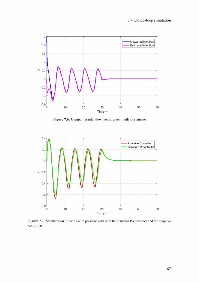
7.4 Closed-loop simulation
0 10 20 30 40 50 60
Time τ
-0.6
-0.4
-0.2
0
0.2
0.4
0.6
0.8
1φ
Measured inlet flowEstimated inlet flow
Figure 7.6: Comparing inlet flow measurement with its estimate
0 10 20 30 40 50 60
Time τ
-0.8
-0.6
-0.4
-0.2
0
0.2
0.4
ψ
Adaptive ControllerStandard P-controller
Figure 7.7: Stabilization of the plenum pressure with both the standard P-controller and the adaptivecontroller
67

7.4 Closed-loop simulation
0 10 20 30 40 50 60
Time τ
-1
-0.5
0
0.5
1
1.5
2
2.5
3k 1
Figure 7.8: Trajectory of the estimate for k1
0 10 20 30 40 50 60
Time τ
0
0.5
1
1.5
2
2.5
3
k 2
Figure 7.9: Trajectory of the estimate for k2
68

7.4 Closed-loop simulation
0 10 20 30 40 50 60
Time τ
5.5
6
6.5
7
7.5
8
8.5
9
9.5
10k 3
Figure 7.10: Trajectory of the estimate for k3
0 10 20 30 40 50 60
Time τ
0.9
0.95
1
1.05
φ0
Figure 7.11: Trajectory of the estimate for φ0
69

7.4 Closed-loop simulation
0 10 20 30 40 50 60
Time τ
0.85
0.9
0.95
1
1.05
1.1ψ
0
Figure 7.12: Trajectory of the estimate for ψ0
Least-squares
By choosing
P0 =
10000 0 00 10000 00 0 10000
and P =
[0.05 0
0 0.04
]
as the initial value for matrix P (for compressor map estimation) and the adaptive gain forequilibrium estimation, the system will response in the following way:
70
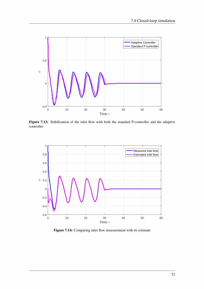
7.4 Closed-loop simulation
0 10 20 30 40 50 60
Time τ
-0.5
0
0.5
1φ
Adaptive ControllerStandard P-controller
Figure 7.13: Stabilization of the inlet flow with both the standard P-controller and the adaptivecontroller
0 10 20 30 40 50 60
Time τ
-0.6
-0.4
-0.2
0
0.2
0.4
0.6
0.8
1
φ
Measured inlet flowEstimated inlet flow
Figure 7.14: Comparing inlet flow measurement with its estimate
71
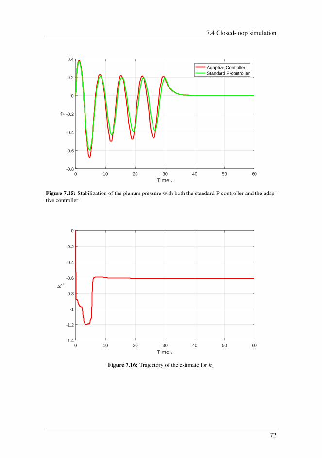
7.4 Closed-loop simulation
0 10 20 30 40 50 60
Time τ
-0.8
-0.6
-0.4
-0.2
0
0.2
0.4ψ
Adaptive ControllerStandard P-controller
Figure 7.15: Stabilization of the plenum pressure with both the standard P-controller and the adap-tive controller
0 10 20 30 40 50 60
Time τ
-1.4
-1.2
-1
-0.8
-0.6
-0.4
-0.2
0
k 1
Figure 7.16: Trajectory of the estimate for k1
72

7.4 Closed-loop simulation
0 10 20 30 40 50 60
Time τ
-1
-0.5
0
0.5
1
1.5
2
2.5
3k 2
Figure 7.17: Trajectory of the estimate for k2
0 10 20 30 40 50 60
Time τ
-1
0
1
2
3
4
5
6
k 3
Figure 7.18: Trajectory of the estimate for k3
73

7.4 Closed-loop simulation
0 10 20 30 40 50 60
Time τ
0.94
0.95
0.96
0.97
0.98
0.99
1
1.01
1.02φ
0
Figure 7.19: Trajectory of the estimate for φ0
0 10 20 30 40 50 60
Time τ
0.84
0.86
0.88
0.9
0.92
0.94
0.96
0.98
1
1.02
1.04
ψ0
Figure 7.20: Trajectory of the estimate for ψ0
7.4.3 Simulations of PAASCSThe controller will be activated at t = 30 in order to prevent the system from oscillating.The controller will be on the form
φu = −B2c2(Ψc − ψ) (7.8)
74

7.4 Closed-loop simulation
where the constant c2 has been chosen to
c2 = k22 − k1 (7.9)
which certainly satisfies the bound:
c1 >k2
2
4k3− k1 (7.10)
since k3 will always have a positive value. The proportional gain is calculated to:
Kp = B2(k22 − k1) = 0.6418(2.82192 − (−0.6192)) = 5.5085 (7.11)
As for the adaptive controller, the controller gain is as follows:
Kpa = B2(k22(t)− k1(t)) (7.12)
where k22(t) and k1(t) are respectively the on-line estimates of k1 and k2 at time t. Those
estimates are being provided either by the method of steepest descent represented byeq.(4.27) or least-squares method represented by equations (4.43) and (4.41). Both es-timation methods are being activated at t = 0. The equations used for constructing theflow observer included to the closed loop are
α = B(Ψc − ψ)− kmωH
φ+kmωH
γT
√ψ
φ = α+ kmVpU
2Aca2o
ψ
(7.13)
In addition, the observer gain has been set to km = 100
Method of Steepest Descent (Gradient Method)
By defining the adaptive gain for the compressor map estimation and equilibrium estima-tion, respectively as
Γ1 =
1500 0 00 275 00 0 100
and P =
[0.05 0
0 0.05
]
the system response in the following way:
75

7.4 Closed-loop simulation
0 10 20 30 40 50 60
Time τ
-0.5
0
0.5
1φ
Adaptive ControllerStandard P-controller
Figure 7.21: Stabilization of the inlet flow with both the standard P-controller and the adaptivecontroller
0 10 20 30 40 50 60
Time τ
-0.6
-0.4
-0.2
0
0.2
0.4
0.6
0.8
1
φ
Measured inlet flowEstimated inlet flow
Figure 7.22: Comparing inlet flow measurement with its estimate
76

7.4 Closed-loop simulation
0 10 20 30 40 50 60
Time τ
-0.8
-0.6
-0.4
-0.2
0
0.2
0.4ψ
Adaptive ControllerStandard P-controller
Figure 7.23: Stabilization of the plenum pressure with both the standard P-controller and the adap-tive controller
0 10 20 30 40 50 60
Time τ
-1
-0.5
0
0.5
1
1.5
2
2.5
3
k 1
Figure 7.24: Trajectory of the estimate for k1
77

7.4 Closed-loop simulation
0 10 20 30 40 50 60
Time τ
0
0.5
1
1.5
2
2.5
3k 2
Figure 7.25: Trajectory of the estimate for k2
0 10 20 30 40 50 60
Time τ
5.5
6
6.5
7
7.5
8
8.5
9
9.5
10
k 3
Figure 7.26: Trajectory of the estimate for k3
78

7.4 Closed-loop simulation
0 10 20 30 40 50 60
Time τ
0.9
0.95
1
1.05φ
0
Figure 7.27: Trajectory of the estimate for φ0
0 10 20 30 40 50 60
Time τ
0.8
0.85
0.9
0.95
1
1.05
1.1
ψ0
Figure 7.28: Trajectory of the estimate for ψ0
Least-squares
By choosing
P0 =
10000 0 00 10000 00 0 10000
and P =
[0.05 0
0 0.04
]
79

7.4 Closed-loop simulation
as the initial value for matrix P and the adaptive gain for equilibrium estimation, the systemwill response in the following way:
0 10 20 30 40 50 60
Time τ
-0.5
0
0.5
1
φ
Adaptive ControllerStandard P-controller
Figure 7.29: Stabilization of the inlet flow with both the standard P-controller and the adaptivecontroller
0 10 20 30 40 50 60
Time τ
-0.6
-0.4
-0.2
0
0.2
0.4
0.6
0.8
1
φ
Measured inlet flowEstimated inlet flow
Figure 7.30: Comparing inlet flow measurement with its estimate
80

7.4 Closed-loop simulation
0 10 20 30 40 50 60
Time τ
-0.8
-0.6
-0.4
-0.2
0
0.2
0.4ψ
Adaptive ControllerStandard P-controller
Figure 7.31: Stabilization of the plenum pressure with both the standard P-controller and the adap-tive controller
0 10 20 30 40 50 60
Time τ
-1.4
-1.2
-1
-0.8
-0.6
-0.4
-0.2
0
k 1
Figure 7.32: Trajectory of the estimate for k1
81

7.4 Closed-loop simulation
0 10 20 30 40 50 60
Time τ
-1
-0.5
0
0.5
1
1.5
2
2.5
3k 2
Figure 7.33: Trajectory of the estimate for k2
0 10 20 30 40 50 60
Time τ
-1
0
1
2
3
4
5
6
k 3
Figure 7.34: Trajectory of the estimate for k3
82

7.4 Closed-loop simulation
0 10 20 30 40 50 60
Time τ
0.94
0.95
0.96
0.97
0.98
0.99
1
1.01
1.02φ
0
Figure 7.35: Trajectory of the estimate for φ0
0 10 20 30 40 50 60
Time τ
0.84
0.86
0.88
0.9
0.92
0.94
0.96
0.98
1
1.02
1.04
ψ0
Figure 7.36: Trajectory of the estimate for ψ0
Evaluation of the results will be done in Section 8 and 9.
83

Chapter 8Discussion
The simulations presented in Chapter 7 arises several issues that requires some attention.
Probably, the most important issue that needs to be discussed is the estimation of the equi-librium point. A study of Figures 7.27, 7.28, 7.35 and 7.36 reveals some gap betweenthe actual coordinates for the equilibrium point and their estimates supplied by the adap-tive law which [6] proposed. This discovery contradicts with the statement made by [6]where one is predicting that θ0 will be equal to x0. The reason for this divergence ispossibly that the model which supplies the adaptive law with system states uses the out-come of the adaptive law itself to compute those states. In fact, a experiment was runby the author where the equilibrium of the system is known beforehand meaning that themodel will generates the states independently of the adaptive law. Under such conditions,the adaptive law produces estimates which manage to exponentially converge to the ac-tual equilibrium. The effect of this inaccuracy in equilibrium estimates will spread to theadaptive controller. Therefore, the performances of the adaptive controller and standardP-controller (for which equilibrium point is known) will differ from each other, even whenk1, k2 and k3 were estimated almost perfectly. Of course, one solution of avoiding sucherror in equilibrium estimates, would be to dismiss the deviation variables in favour ofthe standard variables in order to express the compression system. In return, the devia-tion variables are the key tool in order to obtain a simplified parameter estimation of thecompressor characteristic and cannot simply be omitted. Thus, the uncertainty regardingthe estimation of the equilibrium point is an inevitable drawback of methods introduced inthis thesis.
Comparison of the adaptive and standard P-controller leads to a conclusion that large de-parture of estimates from the actual equilibrium, does not have much of an sizeable in-fluence on the system dynamics. Still, amplitude of surge oscillations tends out be largerfor inaccurate equilibrium estimation than for the case where the equilibrium is known ex-actly. Frequency of the oscillations is the same for both cases. Moreover, the performanceof the adaptive controller seems to be somewhat poorer than it is for the P-controller. Itstill manages, however, to bring the system states exponentially to the origin. Obviously,the are two factors which will influence the performance of the adaptive law: the tuningmatrix P and its initial estimate. In order to get a satisfying result, [6] proposes a slow
84

adaptation (see eq. (3.41)), an advice that has been followed up in this thesis. A reason-able value for the initial estimate can be selected by considering the operating range of thesystem.
Now, the focus is set on the adaptive controller itself. Although some effort has been putin terms of tuning the adaptive gain, there still exist some parameter estimation error θ atsteady-state for both estimation methods. This implies that the fluctuation of mass flow,does not fulfil persistent excitation condition. As the reader may recall from section 4.1,the convergence of θ toward θ∗ is not a priority. Instead, the objective is to come up withsuch estimates so that the the controller drives the system to a stable equilibrium. Based onthe presented simulations in Chapter 7, it can be concluded that the implemented adaptivecontroller satisfies this goal.
The discussion continues to comparing the two estimation methods. Simulations showsthat the estimates reaches their convergence somewhat faster for the gradient method com-pared with least-squares. This result seems to be incidental, but it needs to be noted thatmore care had to be put in tuning the adaptive gain for the gradient method than it did forthe least-squares. As for the latter, the accuracy of the estimates can be improved by bymore aggressively penalizing the estimation error ε; the elements for the initial matrix P0
are set to a very high value. The same approach was tried for the gradient method, only toprovide poorer estimates for the constants k1, k2 and k3. The performance of the adaptivecontroller also worsened. Even if the penalizing of the estimation error with very largematrix P works very well in this particular case of the least-squares, it is not to be expectedin general.
Actually, for all simulations, the gain for the adaptive controller remain constant duringthe stabilization of the system. The reason is that the parameter estimation is being per-formed prior to the activation of the controller. The delay in activating the controller hasbeen incorporated not only to illustrate its effect but also to provide a highly varying flowmeasurement signal for the parameter estimation. Ironically, flow signal oscillating dueto surge, appears to be very well suited for parameter estimation. The suggested adap-tive control embedded for the compression systems can be classified as indirect adaptivecontrol. The hallmark for the indirect adaptive control is that the plant parameters areestimated on-line and later used to compute the controller parameters. [33] mentions thatin academic environments, the indirect adaptive control is being referred to as explicitadaptive control since the design is based on explicit model of the plant. The alternative toindirect adaptive control is obviously direct adaptive control. This strategy is characterizedby parameterizing the plant model in terms of the control parameters which er estimateddirectly ”without intermediate calculations involving plant parameter estimates” as stated[33]. Such approach has been termed implicit adaptive control because the design dependson estimating the implicit plant model.
85

Chapter 9Conclussion
This thesis has provided new results in the field on adaptive control of surge in axial andcentrifugal compressors. Traditional surge controllers often rely on system parameters.Many of them can be regarded as uncertain in special cases. The literature has alreadybeen aware of this uncertainties and have suggested several adaptive controllers that es-timates the unknown parameters and/or updates the control settings so that the systemrequirements are met. In this thesis, two types of surge actuators are being studied: closed-coupled valve (CCV) and a piston. Both actuators were previously operated by standardP-controllers for which the gains can be constructed by the coefficients from the com-pressor map. For a large part of compressor systems, the compressor map will be poorlyknown.
The alternative adaptive controller developed in this work, provided the estimates for thecompressor map by using two very simple identification approaches. Both methodolo-gies generated very accurate estimates and the resulting adaptive controllers managed tostabilize the compression system in a satisfactory way. To apply the suggested estima-tion strategies, however, some specific adjustments had to be done upon the compressormodel. Primarily, the adjustments consisted of expressing the compressor model in termsof deviation variables. Such action required knowledge of the coordinates of the systemequilibrium. If not known, it could either be approximated to some reasonable value orcan explicitly be found by using an adaptive scheme. To the best authors knowledge, suchadaptation scheme has ,until now, newer been used in the context of compressors. Theresults through simulations showed that this methodology had rather poor accuracy or atleast requires a comprehensive amount of tuning. Still, the result were considered suf-ficient for the applications in this thesis. Further research on estimating the compressoroperating point is, however, appreciated and welcomed by the author. The lack of the ac-curacy for the equilibrium estimation would also influence the performance of the adaptivecontroller. For that reason, the adaptive controller differed slightly from the P-controllerwhen it came to stabilizing the compressor. [3mm] The compression system together withthe adaptive controller was also accompanied by the observer which provided the esti-mates of the mass flow for the adaptive controller. The observer was included in bothchoices of actuation. Results showed that the observer provided an very accurate estimatefor mass flow in the case of CCV-actuation. As for the case of assigning the piston as the
86

actuator, the estimate lost its accuracy in the part where the mass flow was recovered fromthe oscillations. However, the overall performance of the observer was still found to beacceptable.
87
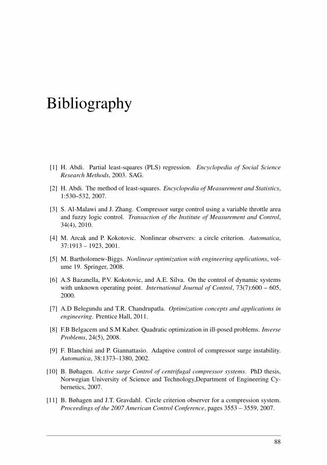
Bibliography
[1] H. Abdi. Partial least-squares (PLS) regression. Encyclopedia of Social ScienceResearch Methods, 2003. SAG.
[2] H. Abdi. The method of least-squares. Encyclopedia of Measurement and Statistics,1:530–532, 2007.
[3] S. Al-Malawi and J. Zhang. Compressor surge control using a variable throttle areaand fuzzy logic control. Transaction of the Institute of Measurement and Control,34(4), 2010.
[4] M. Arcak and P. Kokotovic. Nonlinear observers: a circle criterion. Automatica,37:1913 – 1923, 2001.
[5] M. Bartholomew-Biggs. Nonlinear optimization with engineering applications, vol-ume 19. Springer, 2008.
[6] A.S Bazanella, P.V. Kokotovic, and A.E. Silva. On the control of dynamic systemswith unknown operating point. International Journal of Control, 73(7):600 – 605,2000.
[7] A.D Belegundu and T.R. Chandrupatla. Optimization concepts and applications inengineering. Prentice Hall, 2011.
[8] F.B Belgacem and S.M Kaber. Quadratic optimization in ill-posed problems. InverseProblems, 24(5), 2008.
[9] F. Blanchini and P. Giannattasio. Adaptive control of compressor surge instability.Automatica, 38:1373–1380, 2002.
[10] B. Bøhagen. Active surge Control of centrifugal compressor systems. PhD thesis,Norwegian University of Science and Technology,Department of Engineering Cy-bernetics, 2007.
[11] B. Bøhagen and J.T. Gravdahl. Circle criterion observer for a compression system.Proceedings of the 2007 American Control Conference, pages 3553 – 3559, 2007.
88

BIBLIOGRAPHY
[12] B. Bøhagen, O. Stene, and J.T Gravdahl. A ges flow observer for compression sys-tems: Design and experiment. Proceedings of the 2004 American Control Confer-ence, pages 1528–1533, 2004.
[13] M. Boyce. Axial-flow compressors. boycepower.com, pages 163 – 195.
[14] M. Boyce. Principles of operation and performance estimation of centrifugal com-pressors. Proceedings of the Twenty-Second Turbomachinery Symposium, pages161–177, 1993.
[15] M. Boyce. Centrifugal compressors: a basic guide. PennWell, 2003.
[16] G. Chen and T.T Pham. Fuzzy sets. fuzzy logic and fuzzy control systems. CRC Press,2001.
[17] A. Cortinovis, D. Pareschi, M. Mercangoez, and T. Besselmann. Model predictiveanti-surge control of centrifugal compressors with variable speed drives. Proceedingsof the 2012 IFAC Workshop on Automatic Control in Offshore Oil and Gas Produc-tion, pages 251–256, 2012.
[18] B. de Jager. Rotating stall and surge avoidance: a survey. Proceedings of the 34thIEE Conference on Decition and Control, 2:1857–1862, 1995.
[19] H.W. Emmons, C.E. Pearson, and H.P. Grant. Compressor surge and stall propaga-tion. Transactions of the ASME, 77:455–469, 1955.
[20] A.H Epstein, J.E.F Williams, and E.M Greitzer. Active suppresion of aerodynamicinstabilities in turbomachines. Joournal of Propulsion and Power, 5:204–211, 1989.
[21] J. Felsenstein. An alternating least-squares approach to inferring phylogenies frompairwise distances. Systematic Biology, 46, 1997.
[22] D.A Fink, N.A. Cumpsty, and E.M Greitzer. Surge dynamics in a free-spool cen-reifugal compressor system. Journal of Turbomachinery, 1993.
[23] J.T. Gravdahl. Modeling and control of surge and rotating stall in compressors. PhDthesis, Norwegian University of Science and Technology,Department of EngineeringCybernetics, 1998.
[24] J.T Gravdahl and O. Egeland. Compressor surge control using a closed-coupled valveand backstepping. Proceedings of the American Control Conference, 1997.
[25] J.T Gravdahl and O. Egeland. Compressor surge and rotating stall: modelling andcontrol. Springer, 1999.
[26] J.T Gravdahl and O. Egeland. Modelling and simulation for automatic control. Ma-rine Cybernetics, Trondheim,Norway, 2002.
[27] J.T Gravdahl, O. Egeland, and S.O Vatland. Drive torque actuation is active surgecontrol of centrifugal compressors. Automatica, 38(11):1881–1983, 2002.
[28] E.M. Greitzer. Surge and rotating stall in axial flow compressors, part 1: Theoreticalcompression system model. Journal of Engineering for Power, pages 190–198, 1976.
89

BIBLIOGRAPHY
[29] E.M. Greitzer. Coupled compressor diffuser flow instability. Journal off aircraft,1977.
[30] D. Gysling, D. Dugundji, E. Greitzer, and A. Epstein. Dynamic control of centrifugalcompressor surge using tailored structures. Journal of Turbomachinery, 113(4):710–722, 1991.
[31] K.E Hansen, P. Jørgensen, and P.S Larsen. Experimental and theoretical study ofsurge in a small centrifugal compressor. Journal of Fluids Engineering, 103:391–395, 1991.
[32] A. Ilchmann. Non-identifier-based high gaina adaptive control. Springer, 1993.Lecture Notes in Control and Information Science.
[33] P.A Ioannou and J. Sun. Robust adaptive control. Prentice Hall, 1996.
[34] A. Jerzak. An introduction to centrifugal compressor modelling and load sharing.Norwegian University of Science and Technology,Department of Engineering Cy-bernetics, 2016.
[35] H. Khalil. Nonlinear systems. Prentice Hall, 3rd edition, 2002.
[36] P.V. Kokotovic, H.K. Khalil, and O’Reilly. Singular Pertubation Methods in Control:Analysis and Design. Academic Press, 1986.
[37] K. Louie, H. Clark, and P.C.D Newton. Analysis of differential equation models inbiology: A case study for clover meristem populations. New Zealand Journal ofAgricultural Research, 41:567–576, 1998.
[38] K. Madsen, H.B. Nielsen, and O Tingleff. Methods for non-Linear least-squaresproblems. Informatics and Mathematical Modelling, Technical University of Den-mark, 2nd edition, 2004.
[39] F.K Moore and E.M Greitzer. A theory of post-stall transients in axial compressorsystems: Part i - development of equations. Journal of Engineering for Gas Turbinesand Power, 108:68–76, 1986.
[40] K. Nakagawa, M. Fujiwara, T. Nishioka, S. Tanaka, and Y. Kashiwabara. Experi-mental and numerical analysis of active supression of centrifugal compressor surgeby suction-side valve control. JSME International Journal, Series B, 37(4):878–885,1994.
[41] M.J Nieuwenhuizen. Parameter analysis and identification of the greitzer modelby analogy with the van der pol equation. Master’s thesis, Technische UniversiteitEindhoven,Department Mechanical Engineering, 2008.
[42] T. Øvervag. Centrifugal compressor loadsharing with the use of mpc. Master’sthesis, Norwegian University of Science and Technology,Department of EngineeringCybernetics, 2013.
[43] J.E Pinsley, G.R Guenette, A.H Epstein, and Greitzer E.M. Active stabilization ofcentrifugal compressor surge. Journal of Turbomachinery, 113:723 – 732, 1991.
90

BIBLIOGRAPHY
[44] H. Sheng, W. Huang, T. Zhang, and X. Huang. Robust adaptive control of compressorsurge using backstepping. Arabian Journal of Science and Engineering, 39(12):9301– 9308, 2014.
[45] J.C. Simon, L. Valavani, A.H. Epstein, and E.M Greitzer. Evaluation of approachesto active compressor surge stabilization. Journal of Turbomachinery, 115:57 – 67,1993.
[46] J.S Simon and L. Valavani. A lyapunov based nonlinear control scheme for stabiliz-ing a basic compression system using a closed-coupled control valve. Proceedingsof the 1991 American Control Conference, pages 2398–2406, 1991.
[47] J.F. Slotine and W. Li. Applied non-linear control. Prentice Hall, 1991.
[48] J. Sorokes. Selecting a centrifugal compressor. Chemical Engineering Progress,109(6):44 – 51, 2013.
[49] N. Uddin and J.T. Gravdahl. Piston actuated-surge control of centrifugal compres-sor including integral action. Proceedings og the 11th International Conference onControl, Automation and Systems, 2011a.
[50] N. Uddin and J.T. Gravdahl. Active surge control using pistion actuation. Proceed-ings of the ASM 2011 Dynamic Systems and Control Conference, 2011b.
[51] N. Uddin and J.T Gravdahl. Bond graph modeling of centrifugal compressor systems.Simulations: Transaction of the Society for Modeling and Simulation, 91:998–1013,2015.
[52] N. Uddin and J.T. Gravdahl. Active compressor surge control system by using pis-ton actuation: implementation and experimental results. 11th IFAC Symposium onDynamics and Control of Process Systems, including Biosystems, pages 347 – 352,2016.
[53] N. Uddin and J.T. Gravdahl. Two general feedback control laws for compressorsurge stabilization. 24th Mediterranean Conference on Control and Automation,pages 689–695, 2016.
[54] S. van der Geer. Least-squares estimation. Encyclopedia of Statistics in BehavioralScience, 2:1041–1045, 2005.
[55] N. Westerhof, N. Stergiopulos, and M. Noble. Snapshots of hemodynamics. Springer,2nd edition, 2010.
[56] F. Willems and B. de Jager. Modeling and control of compressor flow instabilities.IEE Control Systems, 19:8–18, 1995.
[57] J.F Williams and X. Huang. Active stabilization of compressor surge. Journal ofFluid Mechanics, 204:245–262, 1989.
[58] S. Yeung and R. Murray. Reduction of bleed valve rate requirements for control ofrotating stall using continous air injection. Proceedingds of the 1997 IEEE Interna-tional Conference on Control Application, pages 693–690, 1997.
91