Simple Harmonic Motion 77

77

Experiment 12: Simple Harmonic Motion

I. About the Experimentost of the information our senses receive about the world in which we live comes to us in the formof waves. Wave motion brings sounds to our ears, light to our eyes, and electromagnetic signals

to our radios and T.V.'s. Wave motion can be defined as the transfer of energy from a source to adistant receiver without the transfer of matter between the two.

Many types of wave motion are generated by different types of mechanical oscillations. One of theleast complicated of these mechanical oscillations is known as simple harmonic motion. In order todevelop an insight into some of the types of forces that control many forms of wave motion we aregoing to examine the simple harmonic motions exhibited by a oscillating spring and a simplependulum.

In order for an object to oscillate it must be acted upon by a force that acts in the opposite direction ofits displacement. If the force is directly proportional to the displacement it is known as a Hooke's Lawforce. Such a force leads to a oscillatory motion that is particularly easy to analyze and the motion isreferred to as Simple Harmonic Motion (SHM).

Thus Simple Harmonic Motion is defined as motion for which the net restoring force is directlyproportional to the displacement away from the equilibrium position,

r F ∝ −

r x . If the position of anobject can be specified by giving just one coordinate (e.g. motion only along a horizontal axis or themotion of a pendulum) we can do away with the vector notation and simply write

F = −kx = ma Eqn. 1

where x is the displacement from the equilibrium position, F is the restoring force (the negative signmeans F and x are opposite in direction), and k is the force constant. This leads to an accelerationgiven by

a = d2xdt 2

= −kmx = −(constant )x Eqn. 2

Any physical system where the acceleration is equal to a negative constant timesthe displacement will move with Simple Harmonic Motion (SHM).The general solution of Equation 2 is

x = A cos(2πft + δ)

4π2 f 2 = km= (constant )

Eqn. 3

You can convince your self that Eqn. 3 solves equation 2 by simply differentiating Eqn. 3 twice.

M

78

The following terms are used to describe SHM:displacement (x) - distance from equilibrium position of the oscillating object at any time t.amplitude (A) - maximum value of displacement. frequency (f) - number of oscillations per unit time.cycle - one complete oscillation of the system. period (T) - time for 1 cycle. T =

1f

phase constant (δ) - the value of δ determines the value of x at t = 0 and the direction of motion at t = 0.

A mass moving vertically on the end of a spring satisfies the conditions for SHM, if we assume that thespring is massless and the displacement of the mass from equilibrium is small. A simple pendulum (allof the pendulums mass is at the end) also satisfies the conditions for SHM if the angle (θ ) thependulum makes with the vertical is small enough that sin(θ ) ≈ θ .

In general for all types of simple harmonic motion the period is given by

T =1f= 2π 1

(constant )Eqn. 4

For a mass m on the end of a (massless) spring of force constant k the period is given by

Tspring = 2π m k Eqn. 5

For a pendulum of length L in a gravitational field g the period is given by

Tpendulum = 2π L g Eqn. 6

where L is the length of the pendulum measured from the top to the center of mass of the bob and g isthe usual acceleration due to gravity. (Equation 6 is for simple pendulum where we assume all the massof the pendulum is a distance L from the pivot point.)

If we square the equations for the periods we obtain

Tspring2 = 4π2m k and Tpendulum

2 = 4π2 L g Eqn. 7

which says that the square of the period for a mass m on the end of a spring is proportional to m andthe square of the period for a pendulum of length L is proportional to L. Thus if we plot T2 vs. m andT2 vs. L on regular graph paper, we should obtain straight lines whose slopes are 4π2/k and 4π2/grespectively.

Simple Harmonic Motion 79

79

II. The Experimental Set-up

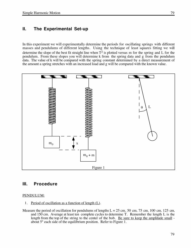
In this experiment we will experimentally determine the periods for oscillating springs with differentmasses and pendulums of different lengths. Using the technique of least squares fitting we willdetermine the slope of the best fit straight line when T2 is plotted versus m for the spring and L for thependulum. From these slopes you will determine k from the spring data and g from the pendulumdata. The value of k will be compared with the spring constant determined by a direct measurement ofthe amount a spring stretches with an increased load and g will be compared with the known value.

+ mm0

m0 x

Lθ

Figure 1

III. Procedure

PENDULUM:

1. Period of oscillation as a function of length (L).

Measure the period of oscillation for pendulums of lengths L = 25 cm, 50 cm, 75 cm, 100 cm, 125 cm,and 150 cm. Average at least ten complete cycles to determine T. Remember the length L is thelength from the top of the string to the center of the bob. Be sure to keep the amplitude small -about 5° each side of the equilibrium position. Refer to Figure 1.

80

SPRING:

2. Direct determination of the force constant k.

Hang your spring with the tapered end up. Place an arbitrary load (m0) on your spring, largeenough to insure that the coils are separated. Add some known mass, m, to this load and measurethe increase in length, x, of the spring. Refer to Figure 1. (Do not stretch your spring close to itselastic limit!)

3. Period of oscillation as a function of mass (m).

Measure the period of oscillation for the spring when the total mass hung from the end of thespring is m = 75 g, 125 g, 175 g, 200 g, 225 g and 250 g Start the oscillation by displacing themass a small distance below the equilibrium position. Average at least ten complete cycles todetermine T.

4. Measure the mass of the spring only.

IV. Calculations and Analysis

1. Enter the data from Part 1II into a spreadsheet and calculate T2. Use the computer to make a plotof T2 versus L.

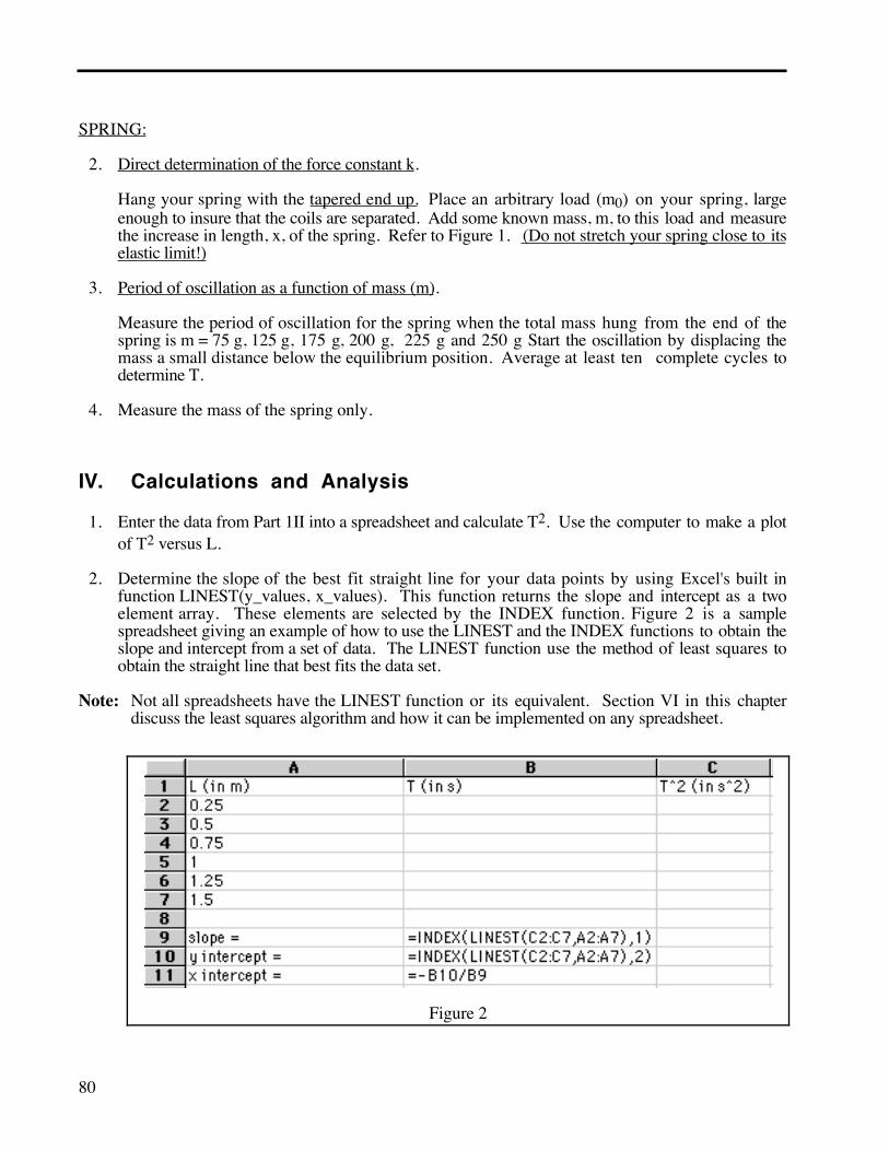
2. Determine the slope of the best fit straight line for your data points by using Excel's built infunction LINEST(y_values, x_values). This function returns the slope and intercept as a twoelement array. These elements are selected by the INDEX function. Figure 2 is a samplespreadsheet giving an example of how to use the LINEST and the INDEX functions to obtain theslope and intercept from a set of data. The LINEST function use the method of least squares toobtain the straight line that best fits the data set.

Note: Not all spreadsheets have the LINEST function or its equivalent. Section VI in this chapterdiscuss the least squares algorithm and how it can be implemented on any spreadsheet.

Figure 2

Simple Harmonic Motion 81

81

3. Determine g from the slope. (Note: slope = 4π2 /g; refer to Equation 7)

4. Compare your calculated value of g to actual value of 9.81m/s2. Note: you are comparing ameasured value to a known value. What do you consider to be the sources of error for thisportion of the experiment?

5. Does your plot pass through the origin? Would you expect it to? Why?

6. From the data of part III.2 calculate k for the spring using k = mgx where m is the additional mass

(i.e. does not include m0).

7. Enter the data from Part III.3 into the same spreadsheet and calculate T2. Use the computer tomake a plot of T2 versus m.

8. Determine the slope of the best fit straight line for your data points by using Excel's built infunction LINEST(y_values, x_values).

9. Calculate k from the slope of your graph (Note: slope = 4π2 /k; refer to Equation 7)

10. Compare the results of 6 and 9. Note: you are comparing two measured values. What do youconsider to be the sources of error for this portion of the experiment?

11. Does your plot pass through the origin?

12. If your plot does not pass through the origin, what is the intercept on the m (x) axis? How doesthis compare with the mass of your spring? What is your explanation for the plot not passingthrough the origin?

V. Questions

1. Must a spring obey Hooke's Law in order to oscillate? Explain.

2. When a body is vibrating in linear simple harmonic motion, is its acceleration zero at any point inthe motion? Where and why?

3. A 70 kg man notices that his 1400 kg car has its center of gravity lowered by 0.50 cm when hegets into it. With what natural frequency would you expect the car to vibrate up and down on itssprings?

4. What is the frequency of a pendulum whose normal period is T when it is in an elevator in freefall?

5. We usually assume the mass of a spring is negligible compared to the mass hung from it. But ifnot negligible, does the mass of the spring increase or decrease the period of motion?

82

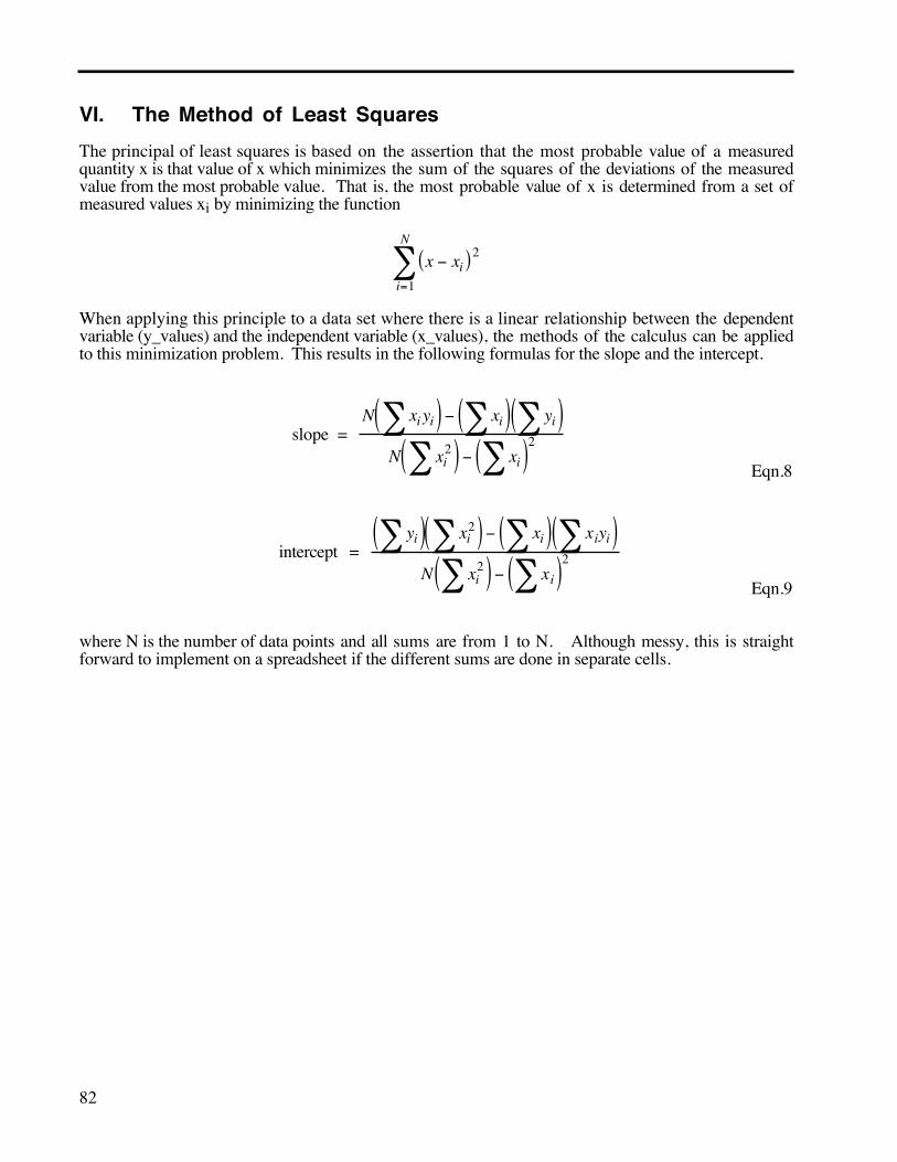
VI. The Method of Least SquaresThe principal of least squares is based on the assertion that the most probable value of a measuredquantity x is that value of x which minimizes the sum of the squares of the deviations of the measuredvalue from the most probable value. That is, the most probable value of x is determined from a set ofmeasured values xi by minimizing the function

x − xi( )2

i=1

N

∑

When applying this principle to a data set where there is a linear relationship between the dependentvariable (y_values) and the independent variable (x_values), the methods of the calculus can be appliedto this minimization problem. This results in the following formulas for the slope and the intercept.

slope = N xi yi∑( ) − xi∑( ) yi∑( )

N xi2∑( ) − xi∑( )2 Eqn.8

intercept = yi∑( ) xi2∑( ) − xi∑( ) xiyi∑( )N xi

2∑( ) − xi∑( )2 Eqn.9

where N is the number of data points and all sums are from 1 to N. Although messy, this is straightforward to implement on a spreadsheet if the different sums are done in separate cells.