Embed Size (px)
Citation preview
14-1©2008 Raj JainCSE567MWashington University in St. Louis
Simple Linear Simple Linear Regression ModelsRegression Models
Raj Jain Washington University in Saint Louis
Saint Louis, MO [email protected]
These slides are available on-line at:http://www.cse.wustl.edu/~jain/cse567-08/
14-2©2008 Raj JainCSE567MWashington University in St. Louis
OverviewOverview
1. Definition of a Good Model2. Estimation of Model parameters3. Allocation of Variation4. Standard deviation of Errors5. Confidence Intervals for Regression Parameters6. Confidence Intervals for Predictions7. Visual Tests for verifying Regression Assumption
14-3©2008 Raj JainCSE567MWashington University in St. Louis
Simple Linear Regression ModelsSimple Linear Regression Models
! Regression Model: Predict a response for a given set of predictor variables.
! Response Variable: Estimated variable! Predictor Variables: Variables used to predict the
response. predictors or factors! Linear Regression Models: Response is a linear
function of predictors. ! Simple Linear Regression Models:
Only one predictor
14-4©2008 Raj JainCSE567MWashington University in St. Louis
Definition of a Good ModelDefinition of a Good Model
x
y
x
y
x
y
x
y
Good Good Bad
14-5©2008 Raj JainCSE567MWashington University in St. Louis
Good Model (Cont)Good Model (Cont)
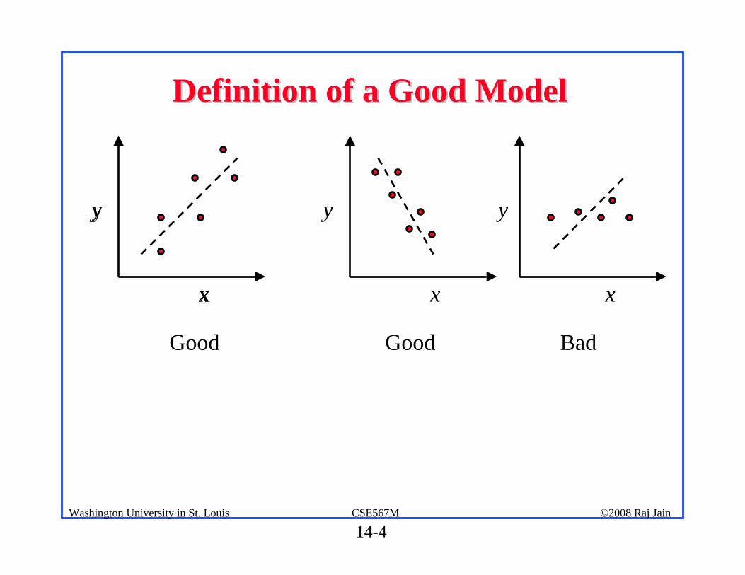
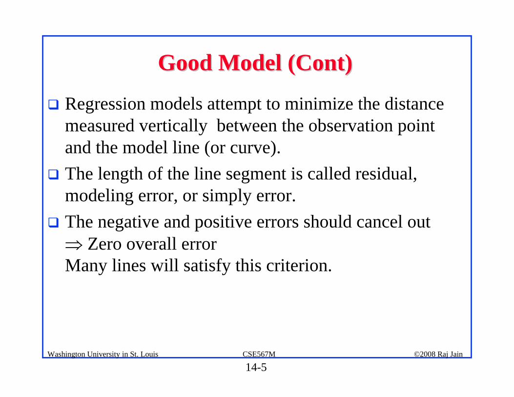
! Regression models attempt to minimize the distance measured vertically between the observation point and the model line (or curve).
! The length of the line segment is called residual, modeling error, or simply error.
! The negative and positive errors should cancel out ⇒ Zero overall error Many lines will satisfy this criterion.
14-6©2008 Raj JainCSE567MWashington University in St. Louis
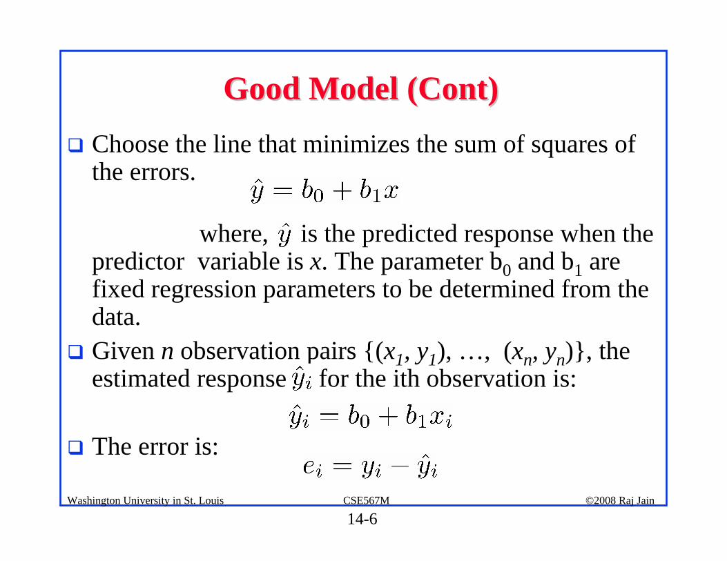
Good Model (Cont)Good Model (Cont)! Choose the line that minimizes the sum of squares of
the errors.
where, is the predicted response when the predictor variable is x. The parameter b0 and b1 are fixed regression parameters to be determined from the data.
! Given n observation pairs {(x1, y1), …, (xn, yn)}, the estimated response for the ith observation is:
! The error is:
14-7©2008 Raj JainCSE567MWashington University in St. Louis
Good Model (Cont)Good Model (Cont)
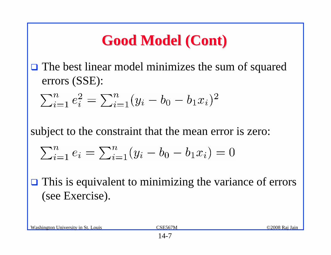
! The best linear model minimizes the sum of squared errors (SSE):
subject to the constraint that the mean error is zero:
! This is equivalent to minimizing the variance of errors (see Exercise).
14-8©2008 Raj JainCSE567MWashington University in St. Louis
Estimation of Model ParametersEstimation of Model Parameters
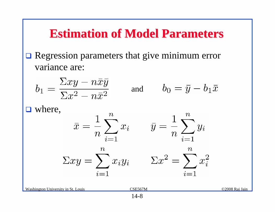
! Regression parameters that give minimum error variance are:
! where,
and
14-9©2008 Raj JainCSE567MWashington University in St. Louis
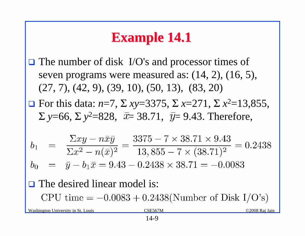
Example 14.1Example 14.1
! The number of disk I/O's and processor times of seven programs were measured as: (14, 2), (16, 5), (27, 7), (42, 9), (39, 10), (50, 13), (83, 20)
! For this data: n=7, Σ xy=3375, Σ x=271, Σ x2=13,855, Σ y=66, Σ y2=828, = 38.71, = 9.43. Therefore,
! The desired linear model is:
14-10©2008 Raj JainCSE567MWashington University in St. Louis
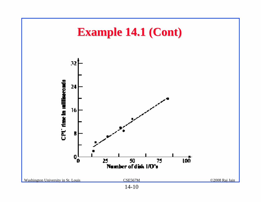
Example 14.1 (Cont)Example 14.1 (Cont)
14-11©2008 Raj JainCSE567MWashington University in St. Louis
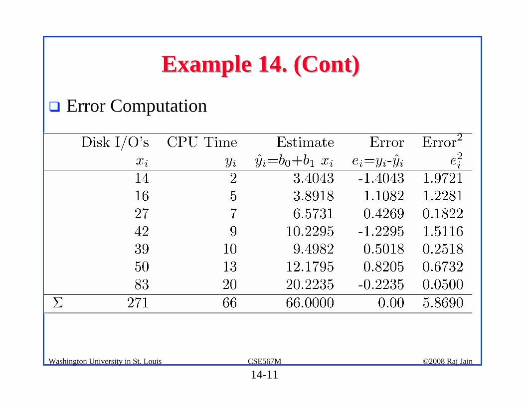
Example 14. (Cont)Example 14. (Cont)
! Error Computation
14-12©2008 Raj JainCSE567MWashington University in St. Louis
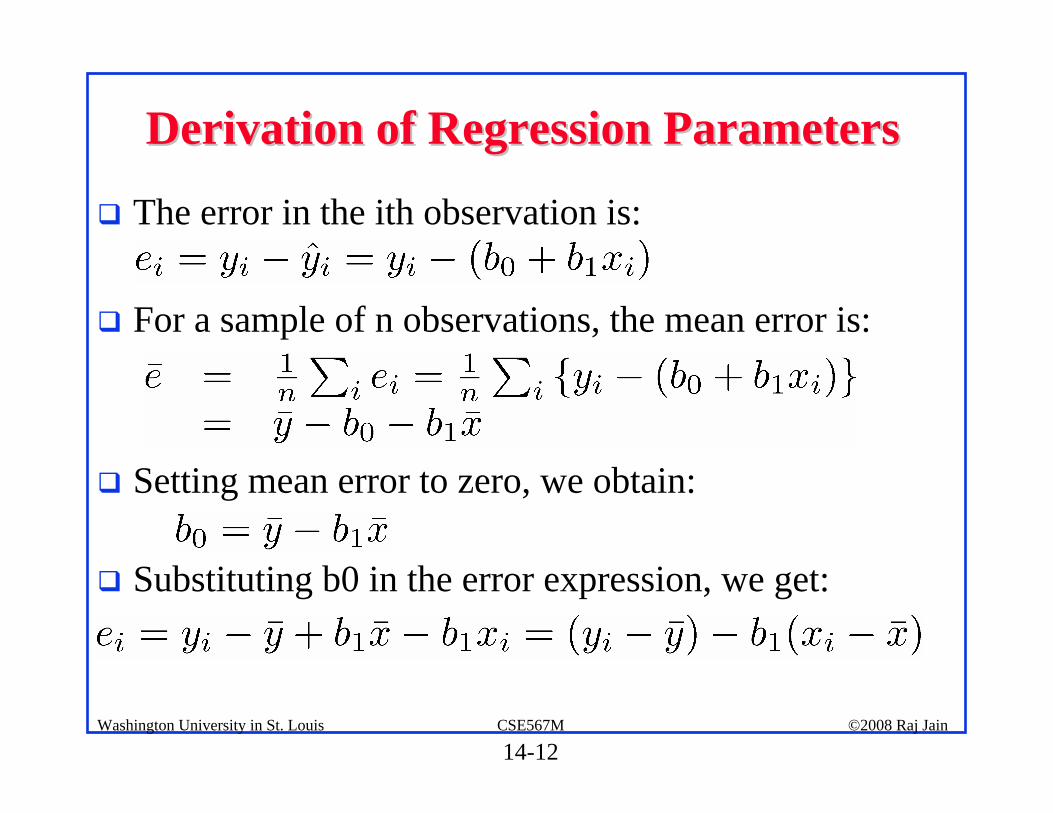
Derivation of Regression ParametersDerivation of Regression Parameters
! The error in the ith observation is:
! For a sample of n observations, the mean error is:
! Setting mean error to zero, we obtain:
! Substituting b0 in the error expression, we get:
14-13©2008 Raj JainCSE567MWashington University in St. Louis
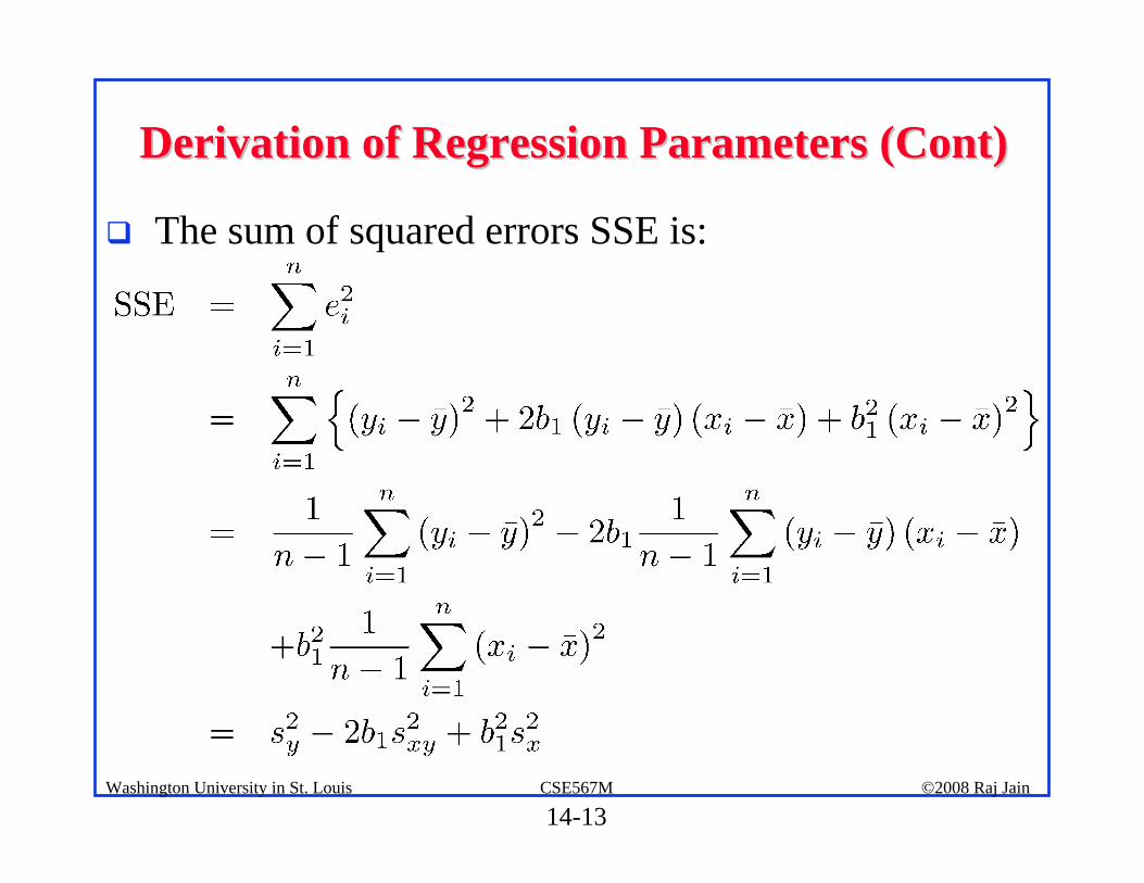
Derivation of Regression Parameters (Cont)Derivation of Regression Parameters (Cont)
! The sum of squared errors SSE is:
14-14©2008 Raj JainCSE567MWashington University in St. Louis
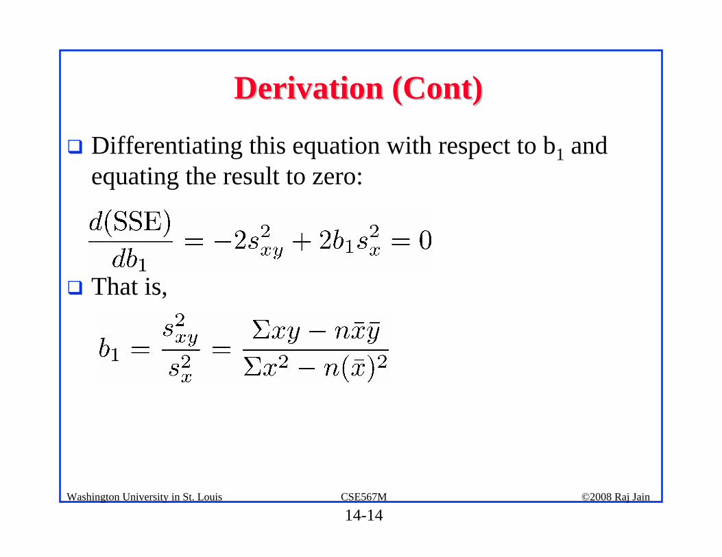
Derivation (Cont)Derivation (Cont)
! Differentiating this equation with respect to b1 and equating the result to zero:
! That is,
14-15©2008 Raj JainCSE567MWashington University in St. Louis
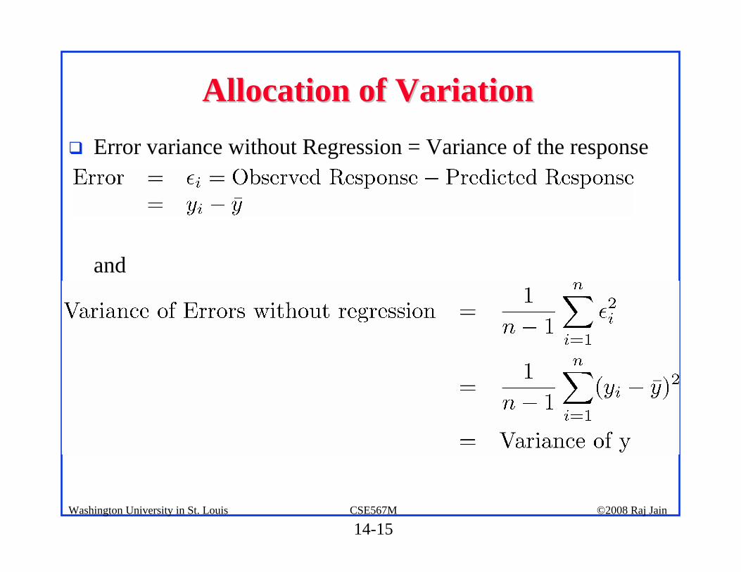
Allocation of VariationAllocation of Variation! Error variance without Regression = Variance of the response
and
14-16©2008 Raj JainCSE567MWashington University in St. Louis
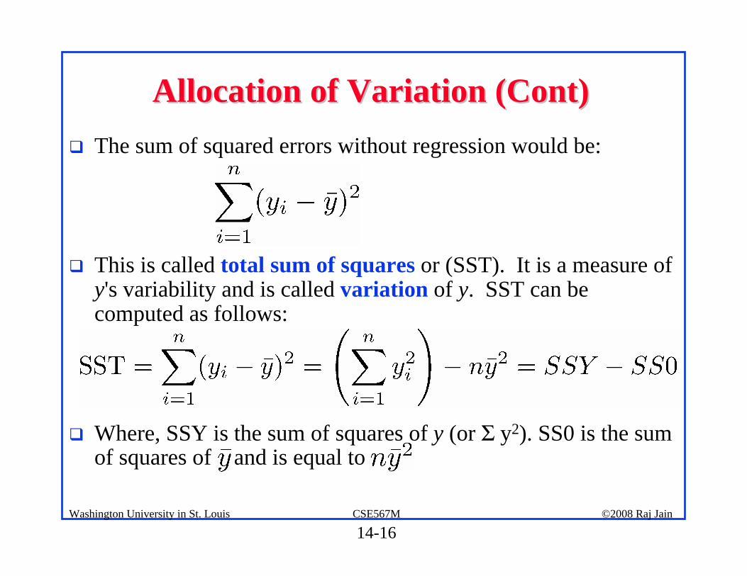
Allocation of Variation (Cont)Allocation of Variation (Cont)! The sum of squared errors without regression would be:
! This is called total sum of squares or (SST). It is a measure of y's variability and is called variation of y. SST can be computed as follows:
! Where, SSY is the sum of squares of y (or Σ y2). SS0 is the sum of squares of and is equal to .
14-17©2008 Raj JainCSE567MWashington University in St. Louis
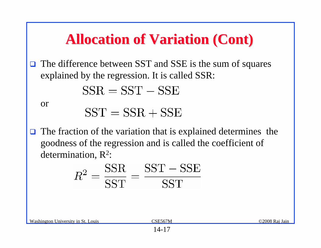
Allocation of Variation (Cont)Allocation of Variation (Cont)! The difference between SST and SSE is the sum of squares
explained by the regression. It is called SSR:
or
! The fraction of the variation that is explained determines the goodness of the regression and is called the coefficient of determination, R2:
14-18©2008 Raj JainCSE567MWashington University in St. Louis
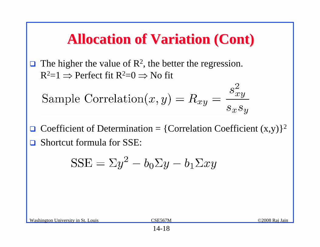
Allocation of Variation (Cont)Allocation of Variation (Cont)! The higher the value of R2, the better the regression.
R2=1 ⇒ Perfect fit R2=0 ⇒ No fit
! Coefficient of Determination = {Correlation Coefficient (x,y)}2
! Shortcut formula for SSE:
14-19©2008 Raj JainCSE567MWashington University in St. Louis
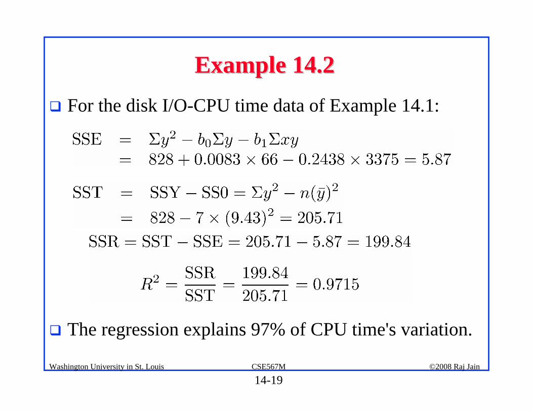
Example 14.2Example 14.2! For the disk I/O-CPU time data of Example 14.1:
! The regression explains 97% of CPU time's variation.
14-20©2008 Raj JainCSE567MWashington University in St. Louis
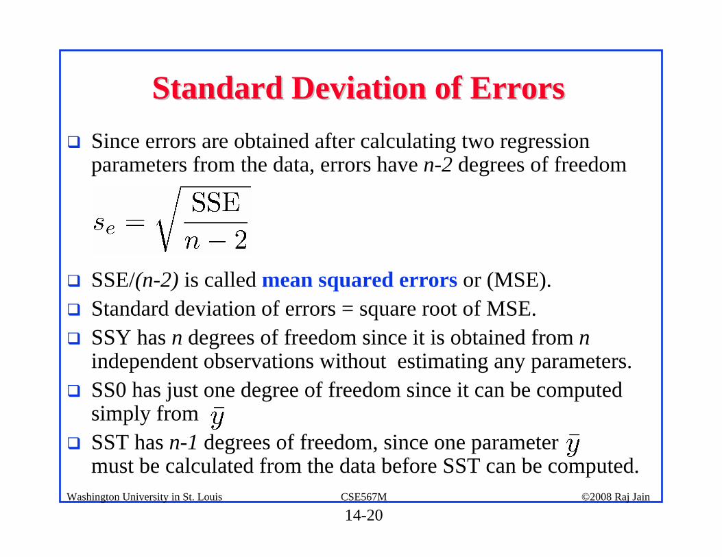
Standard Deviation of ErrorsStandard Deviation of Errors! Since errors are obtained after calculating two regression
parameters from the data, errors have n-2 degrees of freedom
! SSE/(n-2) is called mean squared errors or (MSE). ! Standard deviation of errors = square root of MSE. ! SSY has n degrees of freedom since it is obtained from n
independent observations without estimating any parameters.! SS0 has just one degree of freedom since it can be computed
simply from ! SST has n-1 degrees of freedom, since one parameter
must be calculated from the data before SST can be computed.
14-21©2008 Raj JainCSE567MWashington University in St. Louis
Standard Deviation of Errors (Cont)Standard Deviation of Errors (Cont)
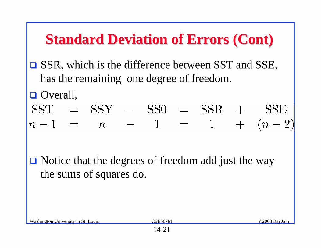
! SSR, which is the difference between SST and SSE, has the remaining one degree of freedom.
! Overall,
! Notice that the degrees of freedom add just the way the sums of squares do.
14-22©2008 Raj JainCSE567MWashington University in St. Louis
Example 14.3Example 14.3
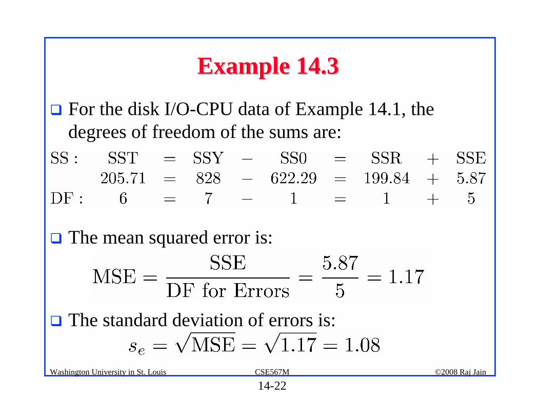
! For the disk I/O-CPU data of Example 14.1, the degrees of freedom of the sums are:
! The mean squared error is:
! The standard deviation of errors is:
14-23©2008 Raj JainCSE567MWashington University in St. Louis
Confidence Intervals for Regression ParamsConfidence Intervals for Regression Params
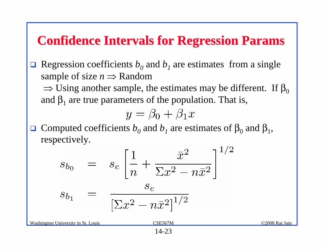
! Regression coefficients b0 and b1 are estimates from a single sample of size n ⇒ Random ⇒ Using another sample, the estimates may be different. If β0
and β1 are true parameters of the population. That is,
! Computed coefficients b0 and b1 are estimates of β0 and β1, respectively.
14-24©2008 Raj JainCSE567MWashington University in St. Louis
Confidence Intervals (Cont)Confidence Intervals (Cont)
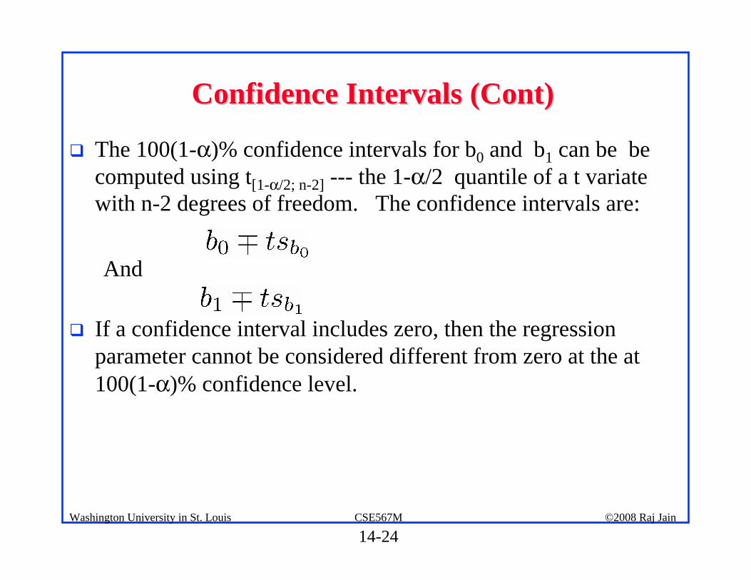
! The 100(1-α)% confidence intervals for b0 and b1 can be be computed using t[1-α/2; n-2] --- the 1-α/2 quantile of a t variate with n-2 degrees of freedom. The confidence intervals are:
And
! If a confidence interval includes zero, then the regression parameter cannot be considered different from zero at the at 100(1-α)% confidence level.
14-25©2008 Raj JainCSE567MWashington University in St. Louis
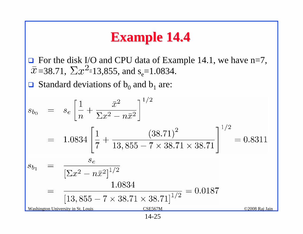
Example 14.4Example 14.4! For the disk I/O and CPU data of Example 14.1, we have n=7,
=38.71, =13,855, and se=1.0834. ! Standard deviations of b0 and b1 are:
14-26©2008 Raj JainCSE567MWashington University in St. Louis
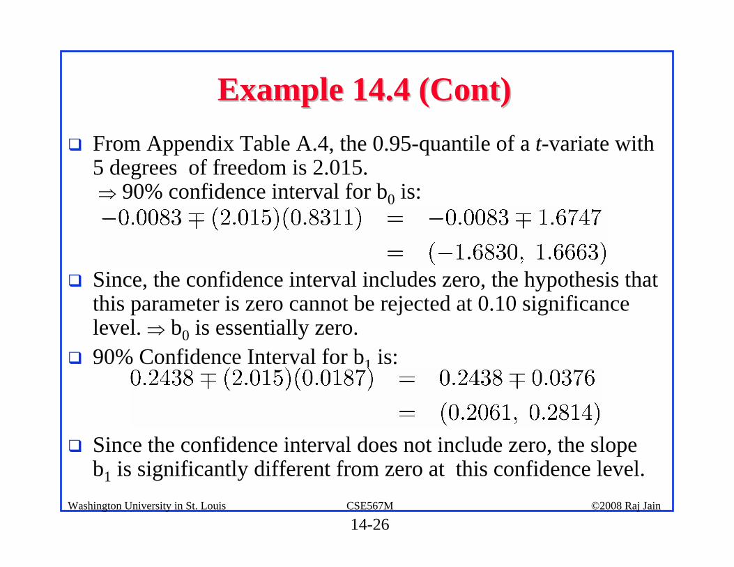
Example 14.4 (Cont)Example 14.4 (Cont)! From Appendix Table A.4, the 0.95-quantile of a t-variate with
5 degrees of freedom is 2.015. ⇒ 90% confidence interval for b0 is:
! Since, the confidence interval includes zero, the hypothesis that this parameter is zero cannot be rejected at 0.10 significance level. ⇒ b0 is essentially zero.
! 90% Confidence Interval for b1 is:
! Since the confidence interval does not include zero, the slope b1 is significantly different from zero at this confidence level.
14-27©2008 Raj JainCSE567MWashington University in St. Louis
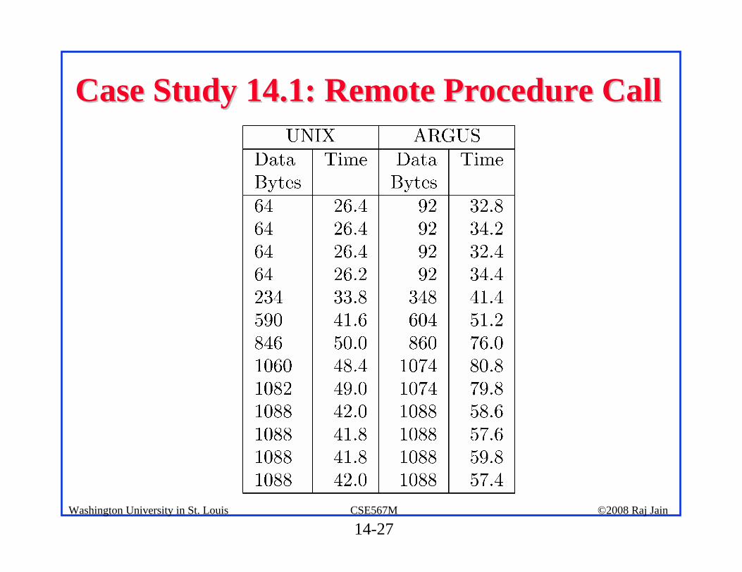
Case Study 14.1: Remote Procedure CallCase Study 14.1: Remote Procedure Call
14-28©2008 Raj JainCSE567MWashington University in St. Louis
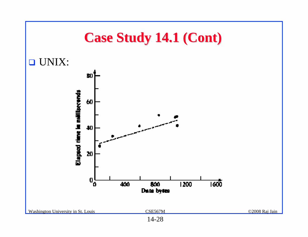
Case Study 14.1 (Cont)Case Study 14.1 (Cont)
! UNIX:
14-29©2008 Raj JainCSE567MWashington University in St. Louis
Case Study 14.1 (Cont)Case Study 14.1 (Cont)
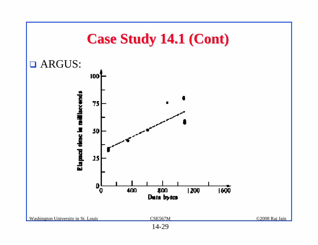
! ARGUS:
14-30©2008 Raj JainCSE567MWashington University in St. Louis
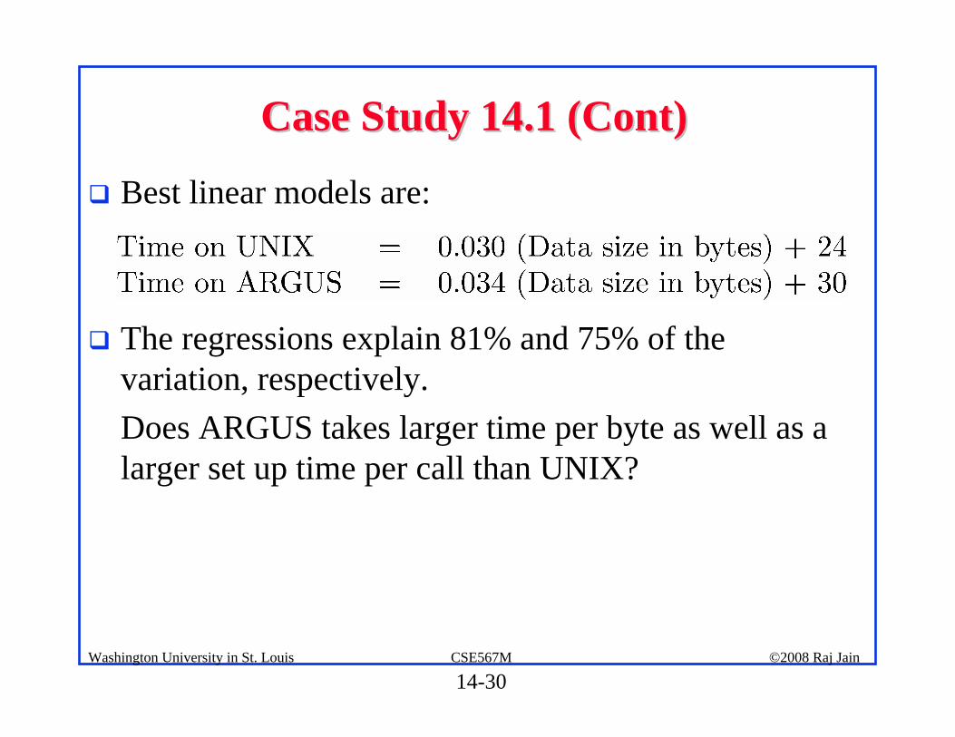
Case Study 14.1 (Cont)Case Study 14.1 (Cont)
! Best linear models are:
! The regressions explain 81% and 75% of the variation, respectively.Does ARGUS takes larger time per byte as well as a larger set up time per call than UNIX?

14-31©2008 Raj JainCSE567MWashington University in St. Louis
Case Study 14.1 (Cont)Case Study 14.1 (Cont)
! Intervals for intercepts overlap while those of the slopes do not. ⇒ Set up times are not significantly different in the two systems while the per byte times (slopes) are different.
14-32©2008 Raj JainCSE567MWashington University in St. Louis
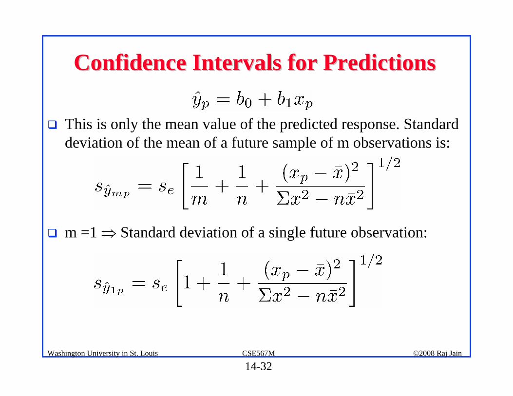
Confidence Intervals for PredictionsConfidence Intervals for Predictions
! This is only the mean value of the predicted response. Standard deviation of the mean of a future sample of m observations is:
! m =1 ⇒ Standard deviation of a single future observation:
14-33©2008 Raj JainCSE567MWashington University in St. Louis
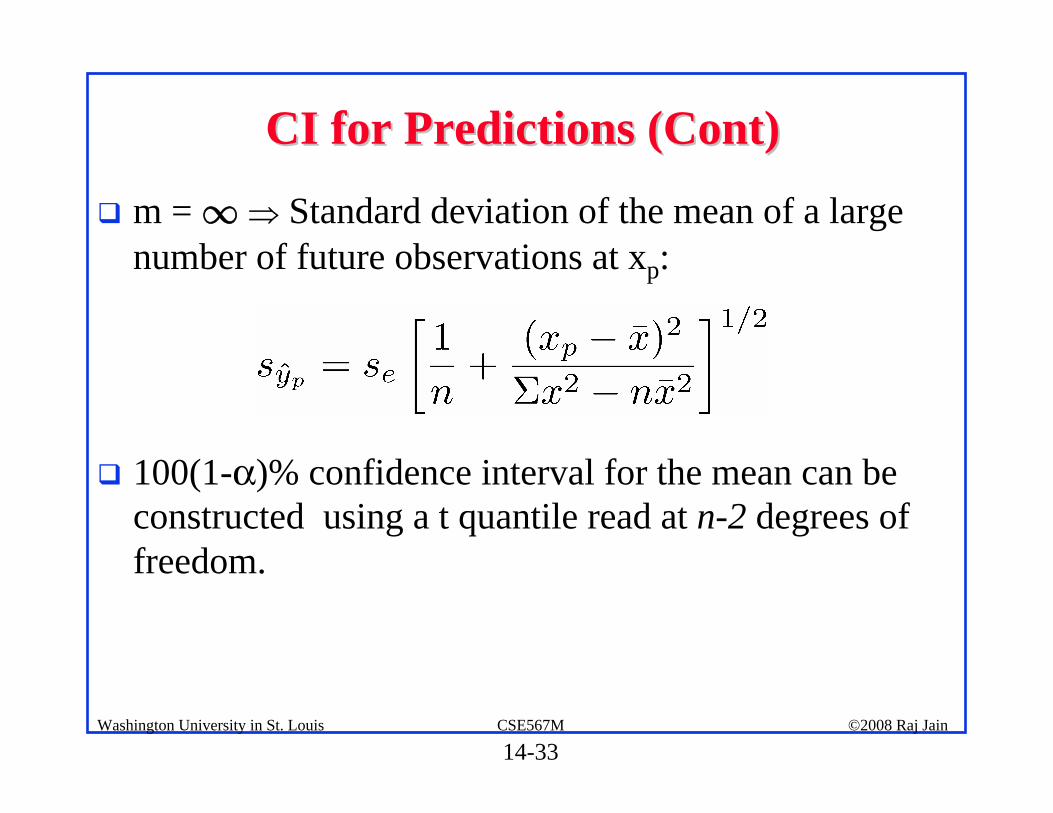
CI for Predictions (Cont)CI for Predictions (Cont)
! m = ∞⇒ Standard deviation of the mean of a large number of future observations at xp:
! 100(1-α)% confidence interval for the mean can be constructed using a t quantile read at n-2 degrees of freedom.
14-34©2008 Raj JainCSE567MWashington University in St. Louis
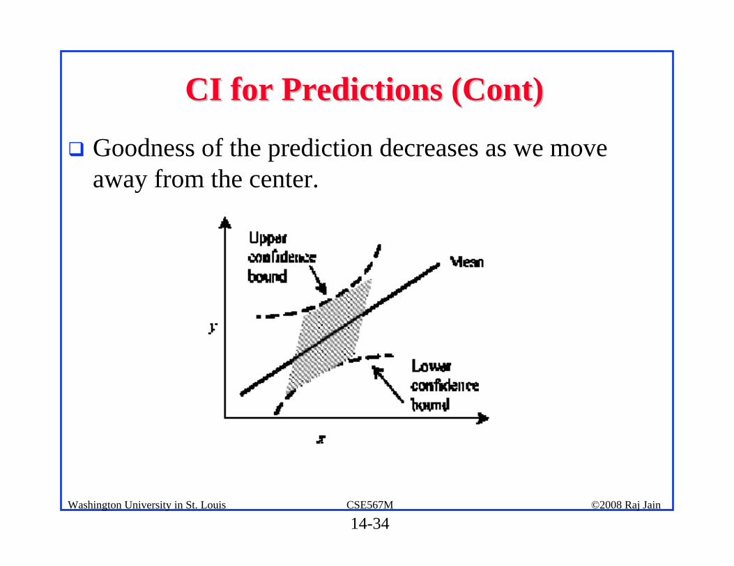
CI for Predictions (Cont)CI for Predictions (Cont)
! Goodness of the prediction decreases as we move away from the center.
14-35©2008 Raj JainCSE567MWashington University in St. Louis
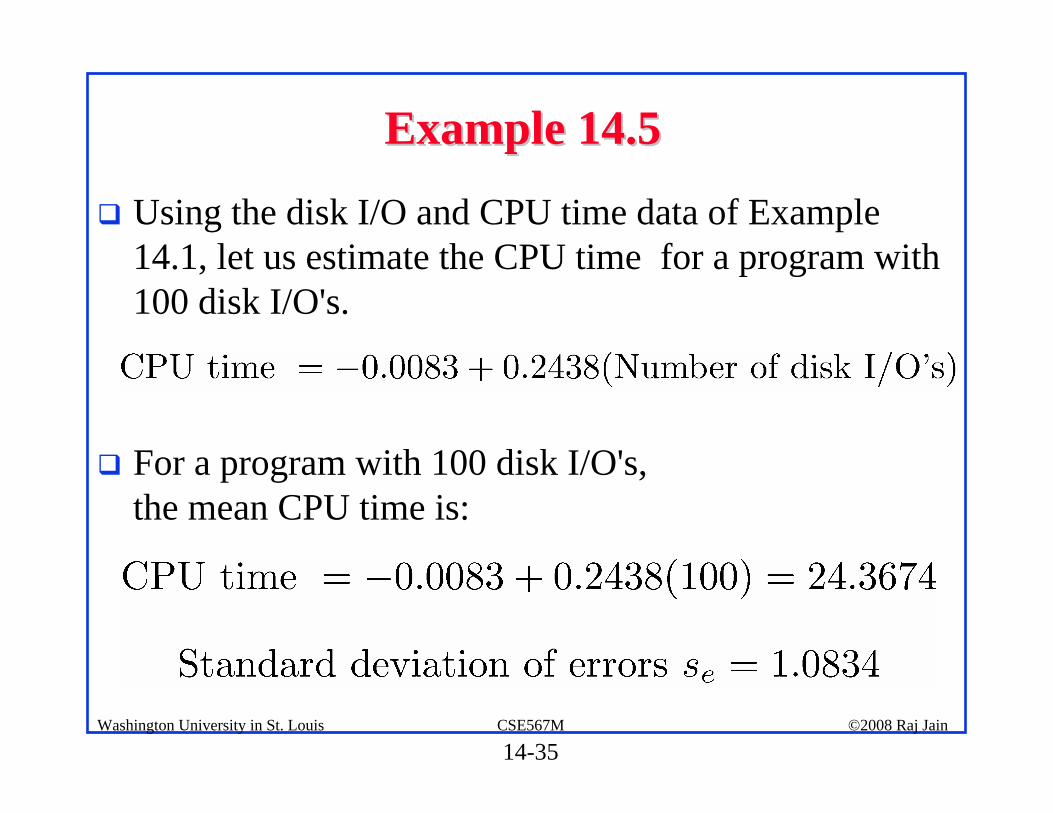
Example 14.5Example 14.5
! Using the disk I/O and CPU time data of Example 14.1, let us estimate the CPU time for a program with 100 disk I/O's.
! For a program with 100 disk I/O's, the mean CPU time is:
14-36©2008 Raj JainCSE567MWashington University in St. Louis
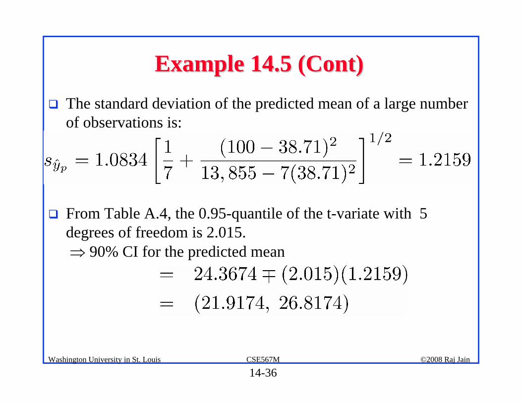
Example 14.5 (Cont)Example 14.5 (Cont)! The standard deviation of the predicted mean of a large number
of observations is:
! From Table A.4, the 0.95-quantile of the t-variate with 5 degrees of freedom is 2.015.⇒ 90% CI for the predicted mean
14-37©2008 Raj JainCSE567MWashington University in St. Louis
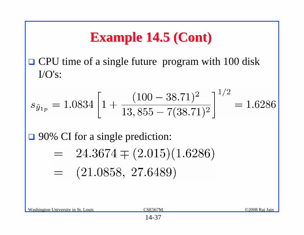
Example 14.5 (Cont)Example 14.5 (Cont)
! CPU time of a single future program with 100 disk I/O's:
! 90% CI for a single prediction:
14-38©2008 Raj JainCSE567MWashington University in St. Louis
Visual Tests for Regression AssumptionsVisual Tests for Regression Assumptions
Regression assumptions:1. The true relationship between the response variable y
and the predictor variable x is linear.2. The predictor variable x is non-stochastic and it is
measured without any error.3. The model errors are statistically independent.4. The errors are normally distributed with zero mean
and a constant standard deviation.
14-39©2008 Raj JainCSE567MWashington University in St. Louis
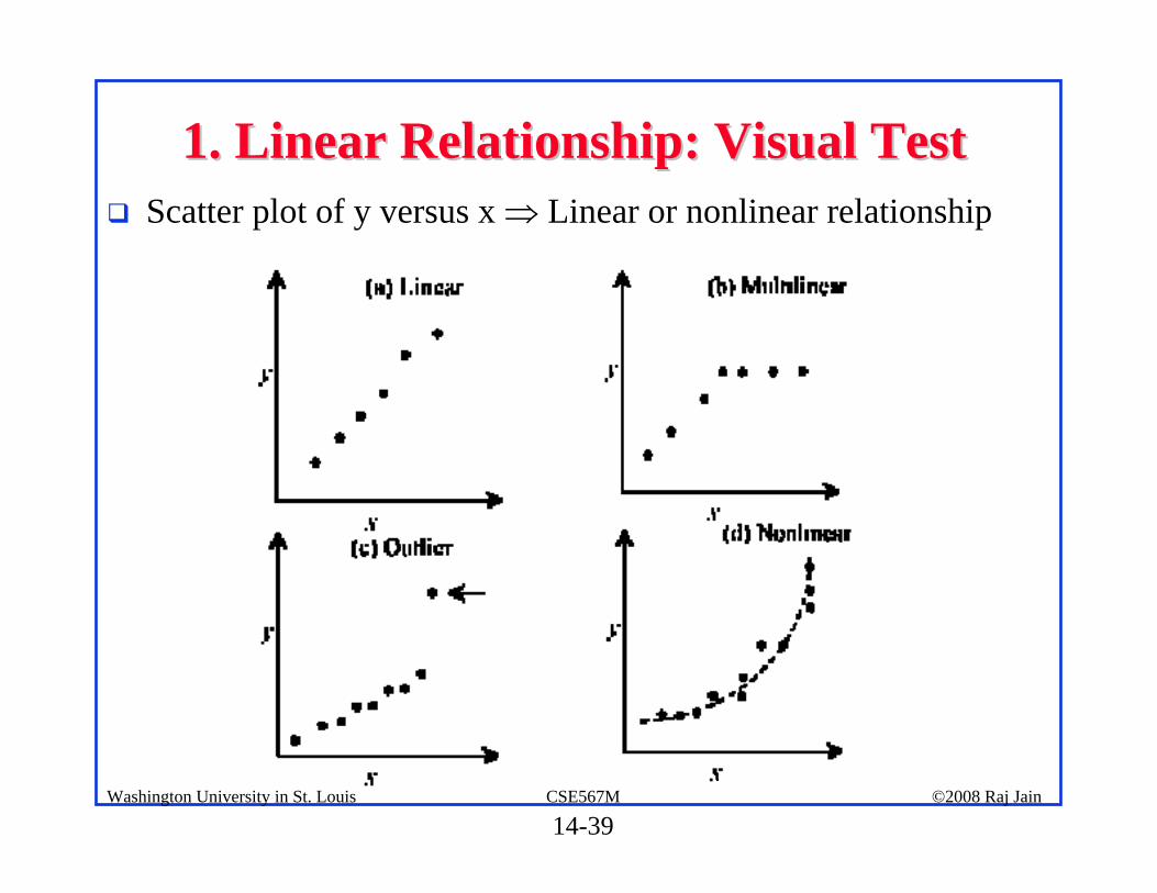
1. Linear Relationship: Visual Test1. Linear Relationship: Visual Test! Scatter plot of y versus x ⇒ Linear or nonlinear relationship
14-40©2008 Raj JainCSE567MWashington University in St. Louis
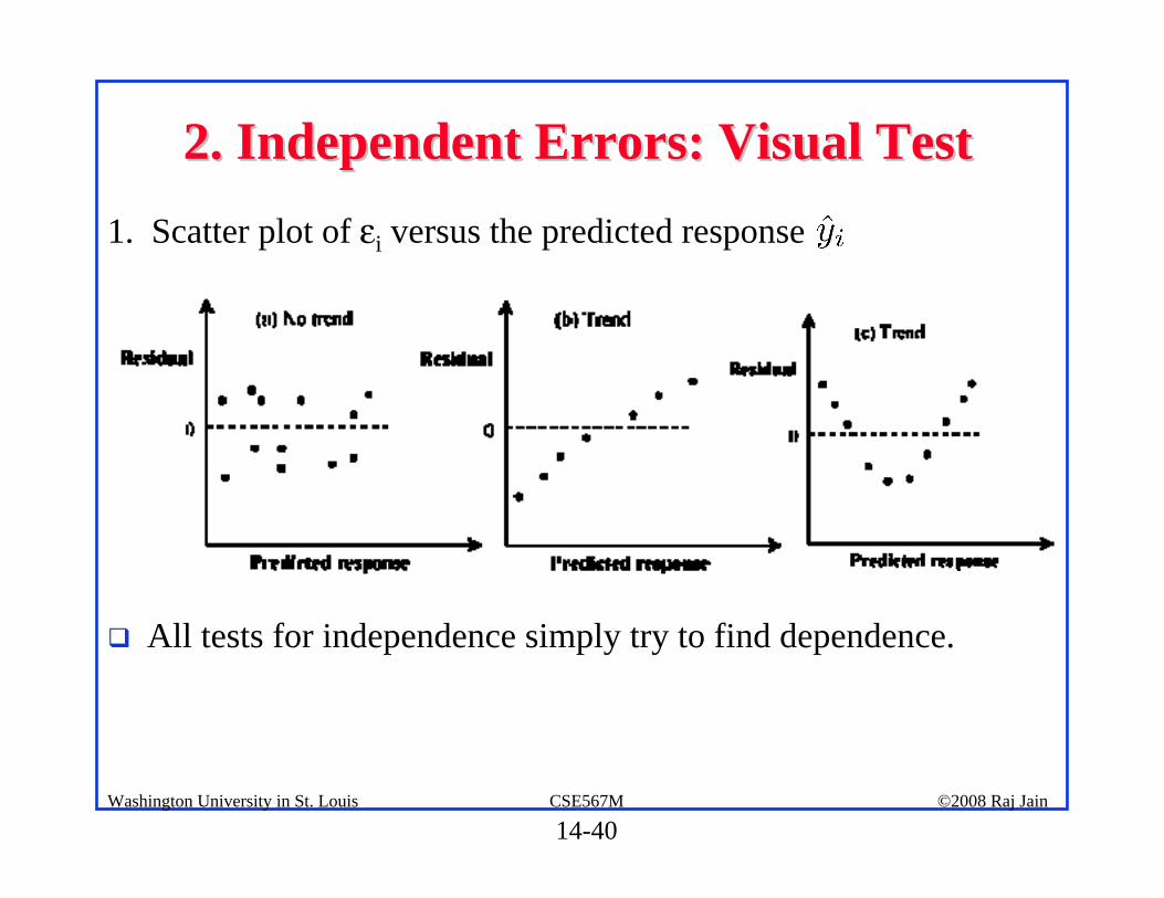
2. Independent Errors: Visual Test2. Independent Errors: Visual Test1. Scatter plot of εi versus the predicted response
! All tests for independence simply try to find dependence.
14-41©2008 Raj JainCSE567MWashington University in St. Louis
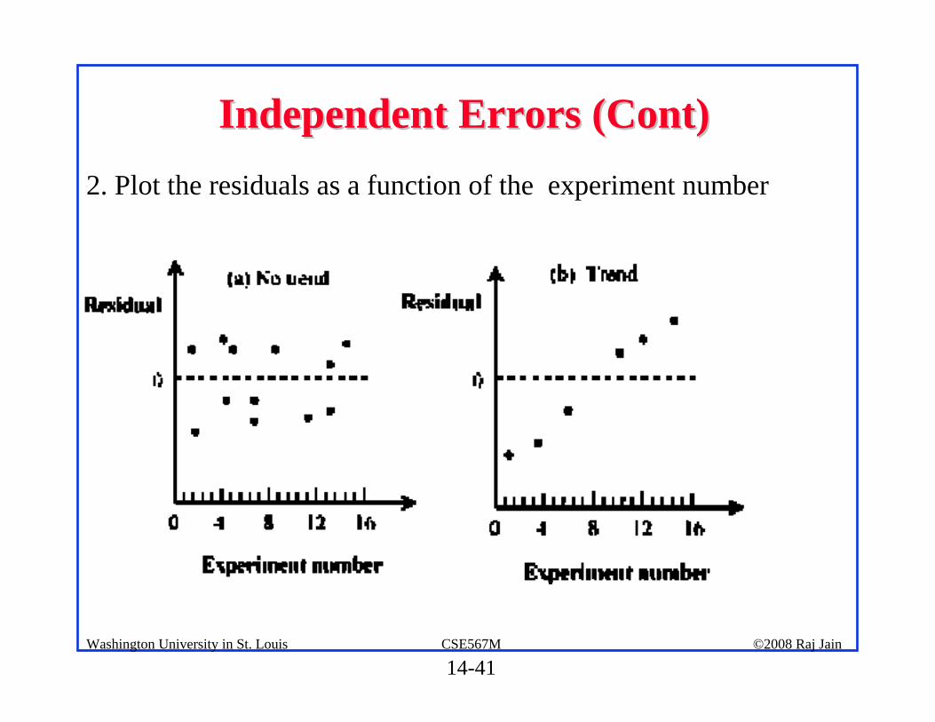
Independent Errors (Cont)Independent Errors (Cont)2. Plot the residuals as a function of the experiment number
14-42©2008 Raj JainCSE567MWashington University in St. Louis
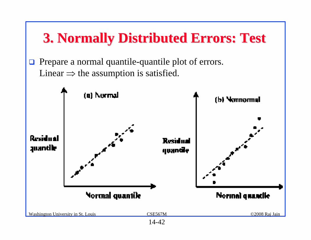
3. Normally Distributed Errors: Test3. Normally Distributed Errors: Test! Prepare a normal quantile-quantile plot of errors.
Linear ⇒ the assumption is satisfied.
14-43©2008 Raj JainCSE567MWashington University in St. Louis
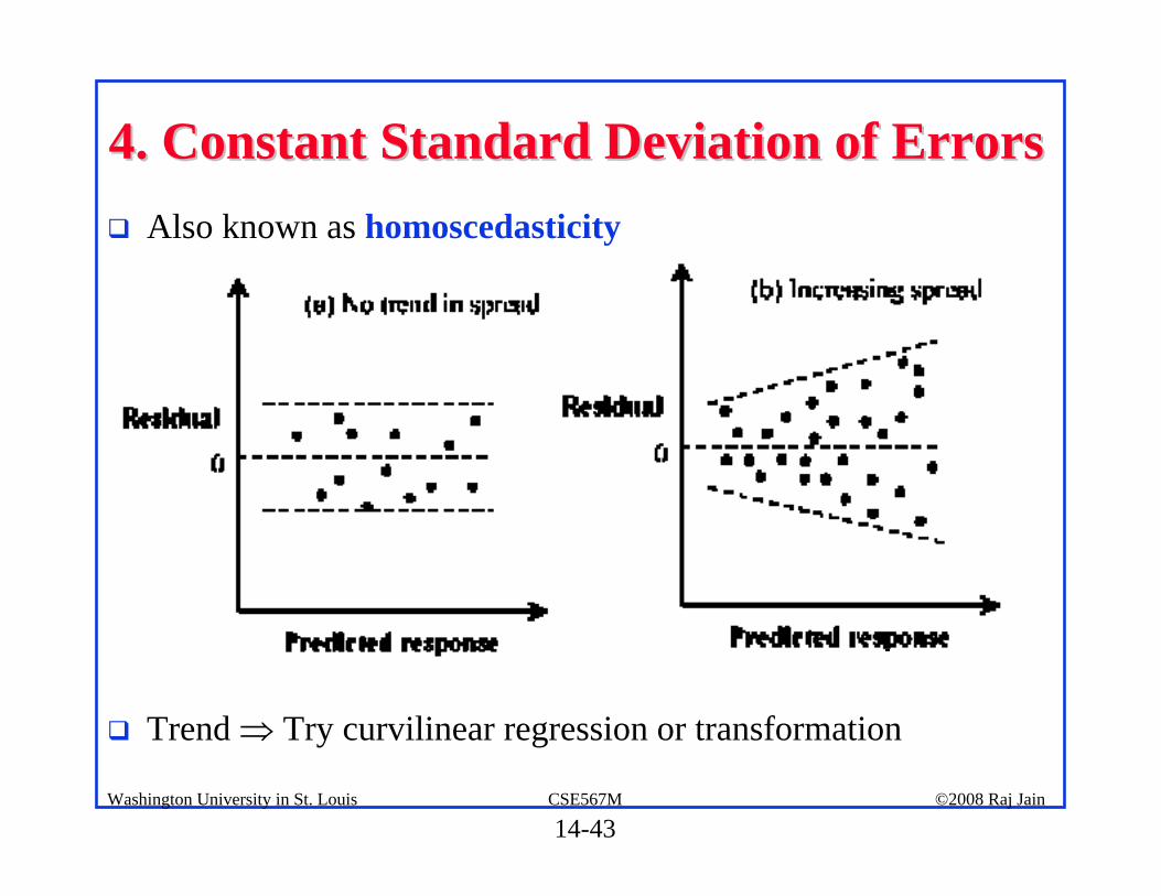
4. Constant Standard Deviation of Errors4. Constant Standard Deviation of Errors! Also known as homoscedasticity
! Trend ⇒ Try curvilinear regression or transformation
14-44©2008 Raj JainCSE567MWashington University in St. Louis
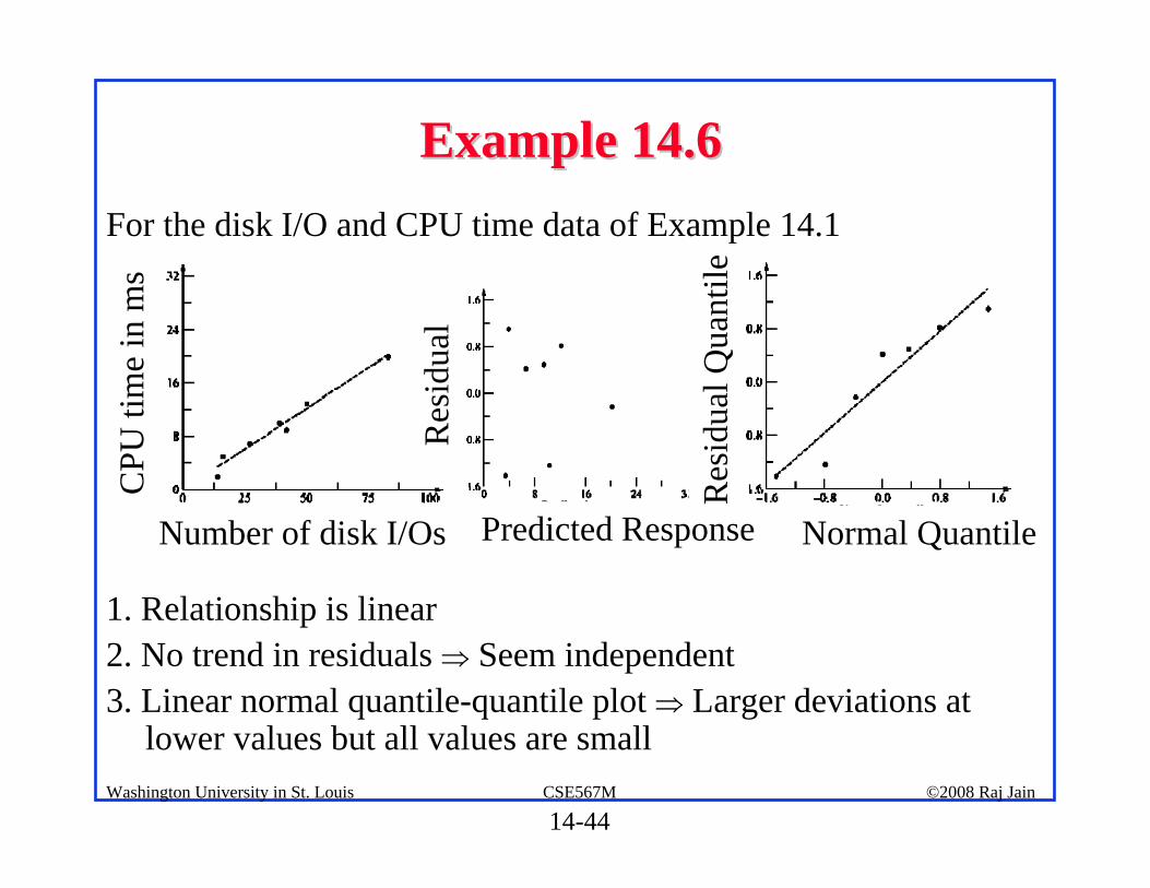
Example 14.6Example 14.6For the disk I/O and CPU time data of Example 14.1
1. Relationship is linear2. No trend in residuals ⇒ Seem independent3. Linear normal quantile-quantile plot ⇒ Larger deviations at
lower values but all values are small
Number of disk I/Os Predicted Response Normal Quantile
CPU
tim
e in
ms
Res
idua
l
Res
idua
l Qua
ntile
14-45©2008 Raj JainCSE567MWashington University in St. Louis
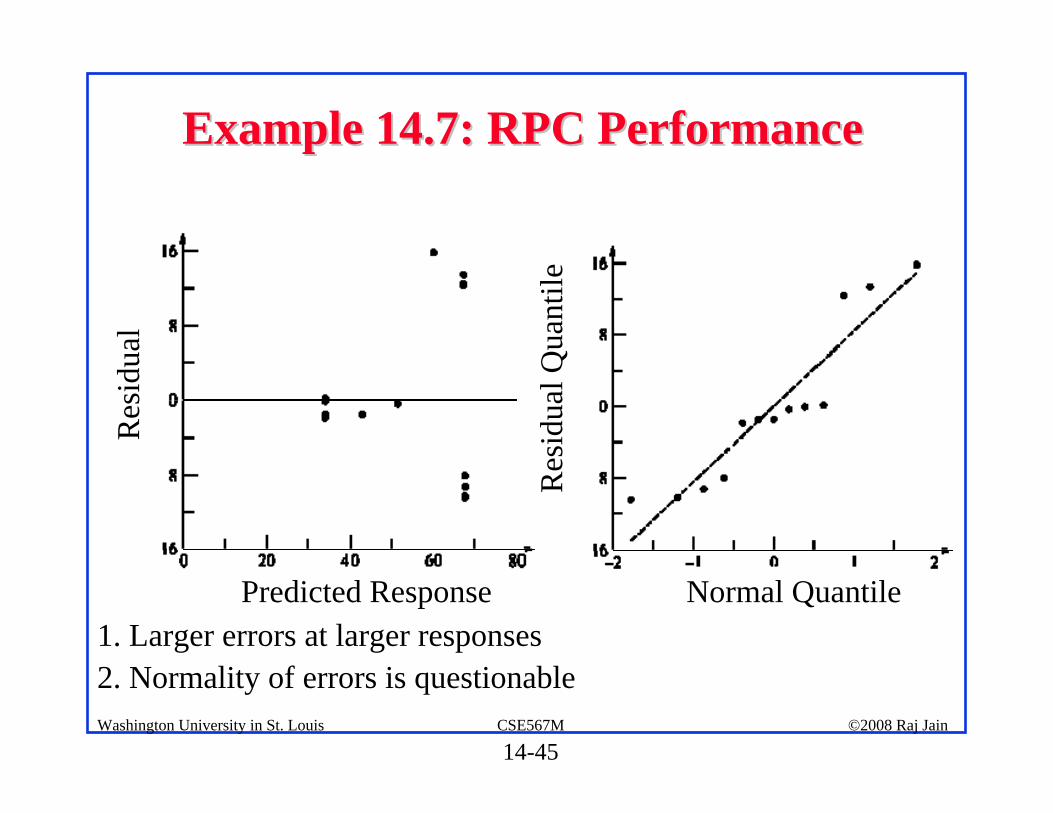
Example 14.7: RPC PerformanceExample 14.7: RPC Performance
1. Larger errors at larger responses2. Normality of errors is questionable
Predicted Response Normal Quantile
Res
idua
l
Res
idua
l Qua
ntile
14-46©2008 Raj JainCSE567MWashington University in St. Louis
SummarySummary
! Terminology: Simple Linear Regression model, Sums of Squares, Mean Squares, degrees of freedom, percent of variation explained, Coefficient of determination, correlation coefficient
! Regression parameters as well as the predicted responses have confidence intervals
! It is important to verify assumptions of linearity, error independence, error normality ⇒ Visual tests
14-53©2008 Raj JainCSE567MWashington University in St. Louis
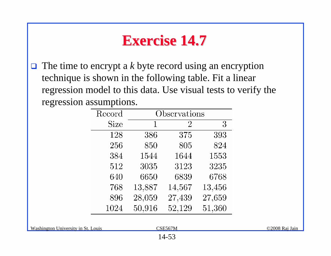
Exercise 14.7Exercise 14.7! The time to encrypt a k byte record using an encryption
technique is shown in the following table. Fit a linear regression model to this data. Use visual tests to verify the regression assumptions.
14-54©2008 Raj JainCSE567MWashington University in St. Louis
Exercise 2.1Exercise 2.1
! From published literature, select an article or a report that presents results of a performance evaluation study. Make a list of good and bad points of the study. What would you do different, if you were asked to repeat the study?
14-55©2008 Raj JainCSE567MWashington University in St. Louis
Homework 14Homework 14
! Read Chapter 14! Submit answers to exercise 14.7! Submit answer to exercise 2.1


