Simple Linear Regression

• Suppose we observe bivariate data (X,Y ), but we do not know the regression functionE(Y |X = x). In many cases it is reasonable to assume that the function is linear:

E(Y |X = x) = α + βx.

In addition, we assume that the distribution is homoscedastic, so that σ(Y |X = x) = σ.

We have reduced the problem to three unknowns (parameters): α, β, and σ. Now we needa way to estimate these unknowns from the data.

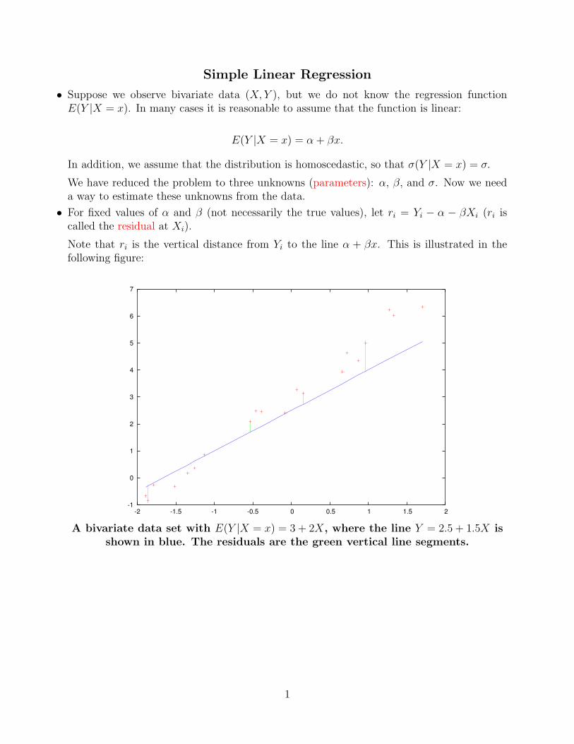
• For fixed values of α and β (not necessarily the true values), let ri = Yi − α − βXi (ri iscalled the residual at Xi).

Note that ri is the vertical distance from Yi to the line α + βx. This is illustrated in thefollowing figure:

-1

0

1

2

3

4

5

6

7

-2 -1.5 -1 -0.5 0 0.5 1 1.5 2

A bivariate data set with E(Y |X = x) = 3 + 2X, where the line Y = 2.5 + 1.5X isshown in blue. The residuals are the green vertical line segments.

1

• One approach to estimating the unknowns α and β is to consider the sum of squared residualsfunction, or SSR.

The SSR is the function∑

i r2i =

∑i(Yi − α − βXi)

2. When α and β are chosen so the fitto the data is good, SSR will be small. If α and β are chosen so the fit to the data is poor,SSR will be large.

-10

-8

-6

-4

-2

0

2

4

6

8

-2 -1.5 -1 -0.5 0 0.5 1 1.5 2-10

-8

-6

-4

-2

0

2

4

6

8

-2 -1.5 -1 -0.5 0 0.5 1 1.5 2

Left: a poor choice of α and β that give high SSR. Right: α and β that givenearly the smallest possible SSR.

• It is a fact that among all possible α and β, the following values minimize the SSR:

β = cov(X, Y )/var(X)

α = Y − βX,

These are called the least squares estimates of α and β.

The estimated regression function is

E(Y |X = x) = α + βx

and the fitted values are

Yi = α + βxi.

2

• Some properties of the least square estimates:

1. β = cor(X, Y )σY /σX , so β and cor(X, Y ) always have the same sign – if thedata are positively correlated, the estimated slope is positive, and if the data arenegatively correlated, the estimated slope is negative.

2. The fitted line α + βx always passes through the overall mean (X, Y ).

3. Since cov(cX, Y ) = c · cov(X, Y ) and var(cX) = c2 · var(X), if we scale the Xvalues by c then the slope is scaled by 1/c. If we scale the Y values by c then theslope is scaled by c.

• Once we have α and β, we can compute the residuals ri based on these estimates, i.e.

ri = Yi − α− βXi.

The following is used to estimate σ:

σ =

√∑i r

2i

n− 2.

• It is also possible to formulate this problem in terms of a model, which is a complete de-scription of the distribution that generated the data.

The model for linear regression is written:

Yi = α + βXi + εi,

where α and β are the population regression coefficients, and the εi are iid random variableswith mean 0 and standard deviation σ. The εi are called errors.

• Model assumptions:

1. The means all fall on the line α + βX.

2. The εi are iid (no heteroscedasticity).

3. The εi have a normal distribution.

Assumption 3 is not always necessary. Least squares estimates α and β are still valid whenthe εi are not normal (as long as 1 and 2 are met).

However hypothesis tests, CI’s, and PI’s (derived below) depend on normality of the εi.

3

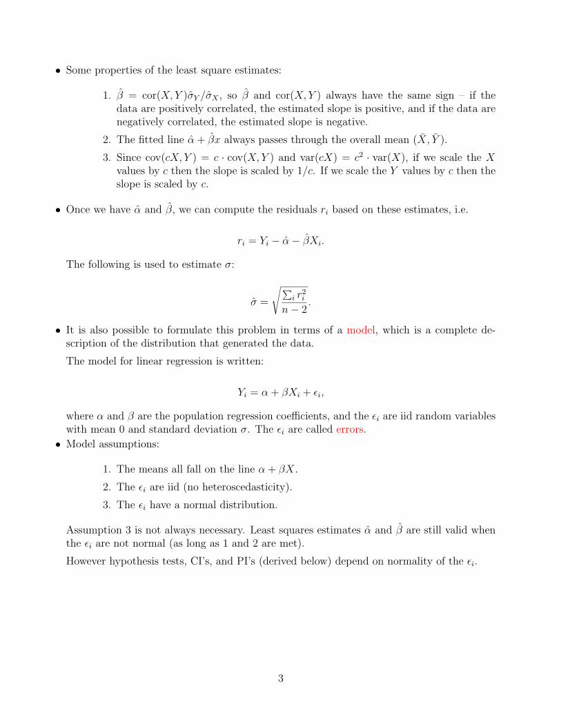
• Since α and β are functions of the data, which is random, they are random variables, andhence they have a distribution.

This distribution reflects the sampling variation that causes α and β to differ somewhat fromthe population values α and β.

The sampling variation is less if the sample size n is large, and if the error standard deviationσ is small.

The sampling variation of β is less if the Xi values are more variable.

We will derive formulas later. For now, we can look at histograms.

0

50

100

150

200

250

300

0 0.5 1 1.5 20

50

100

150

200

250

300

-3 -2.5 -2 -1.5 -1

Sampling variation of α (left) and β (right) for 1000 replicates of the simplelinear model Y = 1− 2X + ε, where SD(ε) = 2, the sample size is n = 200, and

σX ≈ 1.2.

4

0

50

100

150

200

250

0 0.5 1 1.5 20

50

100

150

200

250

300

-3 -2.5 -2 -1.5 -1

Sampling variation of α (left) and β (right) for 1000 replicates of the simplelinear model Y = 1− 2X + ε, where SD(ε) = 1/2, the sample size is n = 200, and

σX ≈ 1.2.

0

50

100

150

200

250

300

0 0.5 1 1.5 20

50

100

150

200

250

300

-3 -2.5 -2 -1.5 -1

Sampling variation of α (left) and β (right) for 1000 replicates of the simplelinear model Y = 1− 2X + ε, where SD(ε) = 2, the sample size is n = 50, and

σX ≈ 1.2.

5

0

50

100

150

200

250

0 0.5 1 1.5 20

50

100

150

200

250

-3 -2.5 -2 -1.5 -1

Sampling variation of α (left) and β (right) for 1000 replicates of the simplelinear model Y = 1− 2X + ε, where SD(ε) = 2, the sample size is n = 50, and

σX ≈ 2.2.

0

50

100

150

200

250

1 1.5 2 2.5 30

50

100

150

200

250

1 1.5 2 2.5 3

Sampling variation of σ for 1000 replicates of the simple linear modelY = 1− 2X + ε, where SD(ε) = 2, the sample size is n = 50 (left) and n = 200

(right), and σX ≈ 1.2.

6

Sampling properties of the least squares estimates

• The following is an identity for the sample covariance:

cov(X, Y ) =1

n− 1

∑i

(Yi − Y )(Xi − X)

=1

n− 1

∑i

YiXi −n

n− 1Y X.

The average of the products minus the product of the averages (almost).A similar identity for the sample variance is

var(Y ) =1

n− 1

∑i

(Yi − Y )2

=1

n− 1

∑i

Y 2i −

n

n− 1Y 2.

The average of the squares minus the square of the averages (almost).

• An identify for the regression model Yi = α + βXi + εi:

1

n

∑Yi =

1

n

∑i

α + βXi + εi

Y = α + βX + ε.

• Let’s get the mean and variance of β:

An equivalent way to write the least squares slope estimate is

β =

∑i YiXi − nY X∑

i X2i − nX2

.

Now if we substitute Yi = α + βXi + εi into the above we get

β =

∑i(α + βXi + εi)Xi − n(α + βX + ε)X∑

i X2i − nX2

.

7

Since

∑i

(α + βXi + εi)Xi = α∑

Xi + β∑

i

X2i +

∑i

εiXi

= nαX + β∑

i

X2i +

∑i

εiXi

we can simplify the expression for β to get

β =β∑

i X2i − nβX2 +

∑i εiXi − nεX∑

i X2i − nX2

,

and further to

β = β +

∑i εiXi − nεX∑i X

2i − nX2

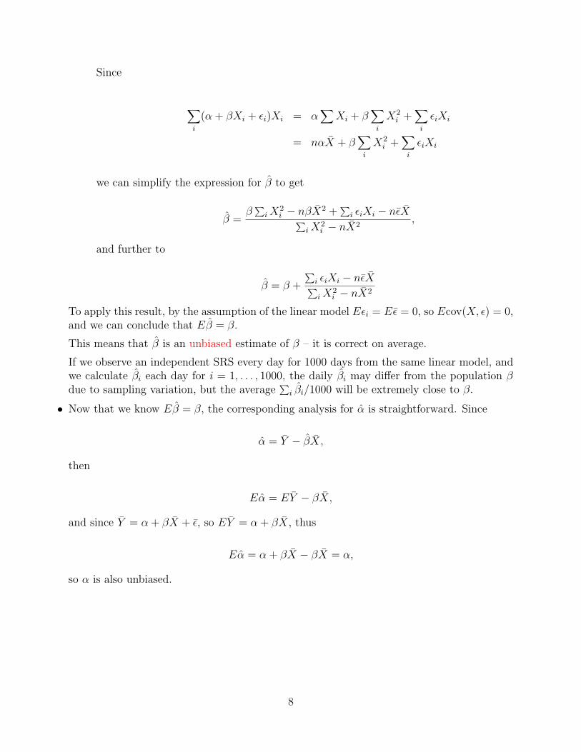
To apply this result, by the assumption of the linear model Eεi = Eε = 0, so Ecov(X, ε) = 0,and we can conclude that Eβ = β.

This means that β is an unbiased estimate of β – it is correct on average.

If we observe an independent SRS every day for 1000 days from the same linear model, andwe calculate βi each day for i = 1, . . . , 1000, the daily βi may differ from the population βdue to sampling variation, but the average

∑i βi/1000 will be extremely close to β.

• Now that we know Eβ = β, the corresponding analysis for α is straightforward. Since

α = Y − βX,

then

Eα = EY − βX,

and since Y = α + βX + ε, so EY = α + βX, thus

Eα = α + βX − βX = α,

so α is also unbiased.

8

• Next we would like to calculate the standard deviation of β, which will allow us to producea CI for β.

Beginning with

β = β +

∑i εiXi − nεX∑i X

2i − nX2

and applying the identity var(U − V ) = var(U) + var(V )− 2cov(U, V ):

var(β) =var(

∑i εiXi) + var(nεX)− 2cov(

∑i εiXi, nεX)

(∑

i X2i − nX2)2

.

Simplifying

var(β) =

∑i X

2i var(εi) + n2X2var(ε)− 2nX

∑i Xicov(εi, ε)

(∑

i X2i − nX2)2

.

Next, using var(εi) = σ2, var(ε) = σ2/n:

var(β) =σ2∑

i X2i + nσ2X2 − 2nX

∑i Xicov(εi, ε)

(∑

i X2i − nX2)2

.

cov(εi, ε) =∑j

cov(εi, εj)/n

= σ2/n.

So we get

var(β) =σ2∑

i X2i + nσ2X2 − 2nX

∑i Xiσ

2/n

(∑

i X2i − nX2)2

=σ2∑

i X2i + nσ2X2 − 2nX2σ2

(∑

i X2i − nX2)2

.

9

Alomst done:

var(β) =σ2∑

i X2i − nX2σ2

(∑

i X2i − nX2)2

=σ2∑

i X2i − nX2

=σ2

(n− 1)var(X),

and

sd(β) =σ√

n− 1σX

.

• The slope SD formula is consistent with the three factors that influenced the precision of βin the histograms:

1. greater sample size reduces the SD

2. greater σ2 increases the SD

3. greater X variability (σX) reduces the SD.

• A similar analysis for α yields

var(α) = σ2

∑X2

i /n

(n− 1)var(X).

Thus var(α) = var(β)∑

X2i /n.

Due to the∑

X2i /n term the estimate will be more precise when the Xi values are close to

zero.

Since α is the intercept, it’s easier to estimate when the data is close to the origin.

• Summary of sampling properties of α, β:

Both are unbiased: Eα = α, Eβ = β.

var(α) = σ2

∑X2

i /n

(n− 1)var(X).

var(β) =σ2

(n− 1)var(X)

Confidence Intervals for β

10

• Start with the basic inequality for standardized β:

P (−1.96 ≤√

n− 1σXβ − β

σ≤ 1.96) = 0.95

then get β alone in the middle:

P (β − 1.96σ√

n− 1σX

≤ β ≤ β + 1.96σ√

n− 1σX

) = .95,

Replace 1.96 with 1.64, etc. to get CI’s with different coverage probabilities.

• Note that in general we will not know σ, so we will need to plug-in σ (defined above) for σ.

This plug-in changes the sampling distribution to tn−2, so to be exact, we would replacethe 1.96 in the above formula with QT (.975), where QT is the quantile function of the tn−2

distribution.

If n is reasonably large, the normal quantile will be an excellent approximation.

0

1

2

3

4

5

6

-2 -1.5 -1 -0.5 0 0.5 1 1.5 2

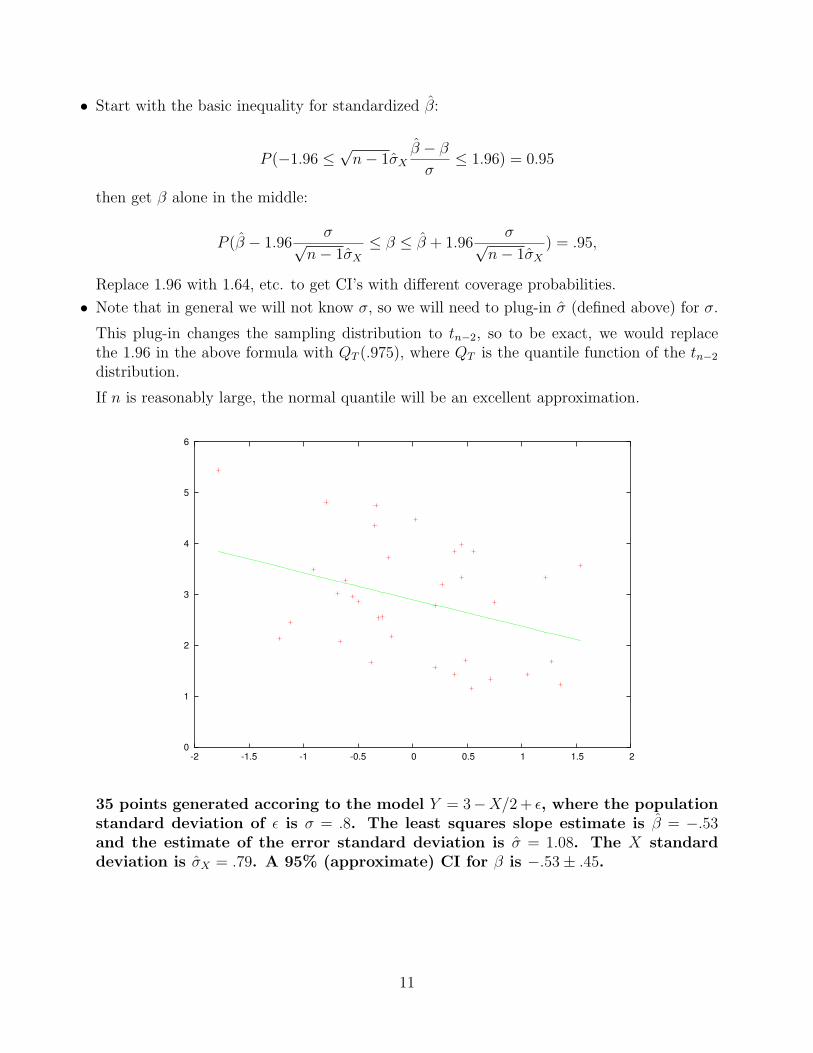
35 points generated accoring to the model Y = 3−X/2 + ε, where the populationstandard deviation of ε is σ = .8. The least squares slope estimate is β = −.53and the estimate of the error standard deviation is σ = 1.08. The X standarddeviation is σX = .79. A 95% (approximate) CI for β is −.53± .45.

11

0

1

2

3

4

5

6

-2 -1.5 -1 -0.5 0 0.5 1 1.5 2

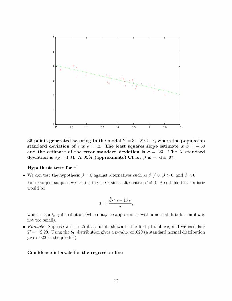
35 points generated accoring to the model Y = 3−X/2 + ε, where the populationstandard deviation of ε is σ = .2. The least squares slope estimate is β = −.50and the estimate of the error standard deviation is σ = .23. The X standarddeviation is σX = 1.04. A 95% (approximate) CI for β is −.50± .07.

Hypothesis tests for β

• We can test the hypothesis β = 0 against alternatives such as β 6= 0, β > 0, and β < 0.

For example, suppose we are testing the 2-sided alternative β 6= 0. A suitable test statisticwould be

T =β√

n− 1σX

σ,

which has a tn−2 distribution (which may be approximate with a normal distribution if n isnot too small).

• Example: Suppose we the 35 data points shown in the first plot above, and we calculateT = −2.29. Using the t33 distribution gives a p-value of .029 (a standard normal distributiongives .022 as the p-value).

Confidence intervals for the regression line

12

• The fitted value at X, denoted Y , is the Y coordinate of the estimated regression line at X:

Y = α + βX

The fitted value is an estimate of the regression function E(Y |X) evaluated at the point X,so we may also write E(Y |X).

Fitted values may be calculated at any X value. If X is one of the observed X values, sayX = Xi, write Yi = α + βXi.

• Since Yi is a random variable, we can calculate its mean and variance.

To get the mean, recall that Eα = α and Eβ = β. Therefore

EYi = E(α + βXi)

= Eα + Eβ ·Xi

= α + βXi

= EYi

Thus Yi is an unbiased estimate of E(Y |X) evaluated at X = Xi.

• To calculate the variance, begin with the following:

varYi = var(α + βXi)

= varα + var(βXi) + 2cov(α, βXi)

= varα + X2i varβ + 2Xicov(α, β)

= σ2(σ2X + X2)/nσ2

X + X2i σ2/nσ2

X + 2Xicov(α, β)

To derive cov(α, β), similar techniques as were used to calculate varα and varβ can beapplied. The result is

cov(α, β) = −σ2X

nσ2X

.

13

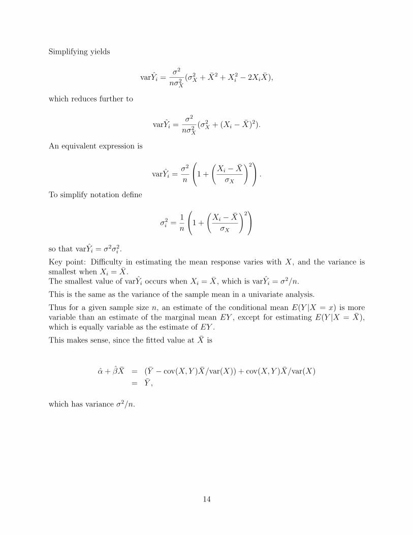
Simplifying yields

varYi =σ2

nσ2X

(σ2X + X2 + X2

i − 2XiX),

which reduces further to

varYi =σ2

nσ2X

(σ2X + (Xi − X)2).

An equivalent expression is

varYi =σ2

n

1 +

(Xi − X

σX

)2 .

To simplify notation define

σ2i =

1

n

1 +

(Xi − X

σX

)2

so that varYi = σ2σ2i .

Key point: Difficulty in estimating the mean response varies with X, and the variance issmallest when Xi = X.The smallest value of varYi occurs when Xi = X, which is varYi = σ2/n.

This is the same as the variance of the sample mean in a univariate analysis.

Thus for a given sample size n, an estimate of the conditional mean E(Y |X = x) is morevariable than an estimate of the marginal mean EY , except for estimating E(Y |X = X),which is equally variable as the estimate of EY .

This makes sense, since the fitted value at X is

α + βX = (Y − cov(X, Y )X/var(X)) + cov(X, Y )X/var(X)

= Y ,

which has variance σ2/n.

14

• We now know the mean and variance of Yi. Standardizing yields

P (−1.96 ≤ Yi − (α + βXi)

σσi

≤ 1.96) = .95,

equivalently

P (Yi − 1.96σσi ≤ α + βXi ≤ Yi + 1.96σσi) = .95.

This gives a 95% CI for EYi.

• Since σ is unknown we must plug-in σ for σ in the CI. Thus we get the approximate CI

P (Yi − 1.96σσi ≤ α + βXi ≤ Yi + 1.96σσi) ≈ 0.95.

We can make the coverage probability exactly 0.95 by using the tn−2 distribution to calculatequantiles:

P (Yi −Q(0.975)σσi ≤ α + βXi ≤ Yi + Q(0.975)σσi) = 0.95.

• The following show CI’s for the population regression function E(Y |X). In each data figure,a CI is formed for each Xi value. Note that the goal of each CI is to cover the green line,and this should happen 95% of the time.

Note also that the CI’s are narrower for Xi close to X compared to Xi that are far from X.Also note that the CI’s are longer when σ is greater.

15

-8

-7

-6

-5

-4

-3

-2

-1

-2 -1.5 -1 -0.5 0 0.5 1 1.5

The red points are a bivariate data set generated according to the model Y =−4 + 1.4X + ε, where SD(ε) = .4. The green line is the population regressionfunction, the blue line is the fitted regression function, and the vertical bluebars show 95% CI’s for E(Y |X = Xi) at each Xi value.

16

-7

-6

-5

-4

-3

-2

-1

-2 -1.5 -1 -0.5 0 0.5 1 1.5 2

The red points are a bivariate data set generated according to the model Y =−4 + 1.4X + ε, where SD(ε) = 1. The green line is the population regressionfunction, the blue line is the fitted regression function, and the vertical bluebars show 95% CI’s for E(Y |X = Xi) at each Xi value.

17

-8

-7

-6

-5

-4

-3

-2

-1

0

-2 -1.5 -1 -0.5 0 0.5 1 1.5 2

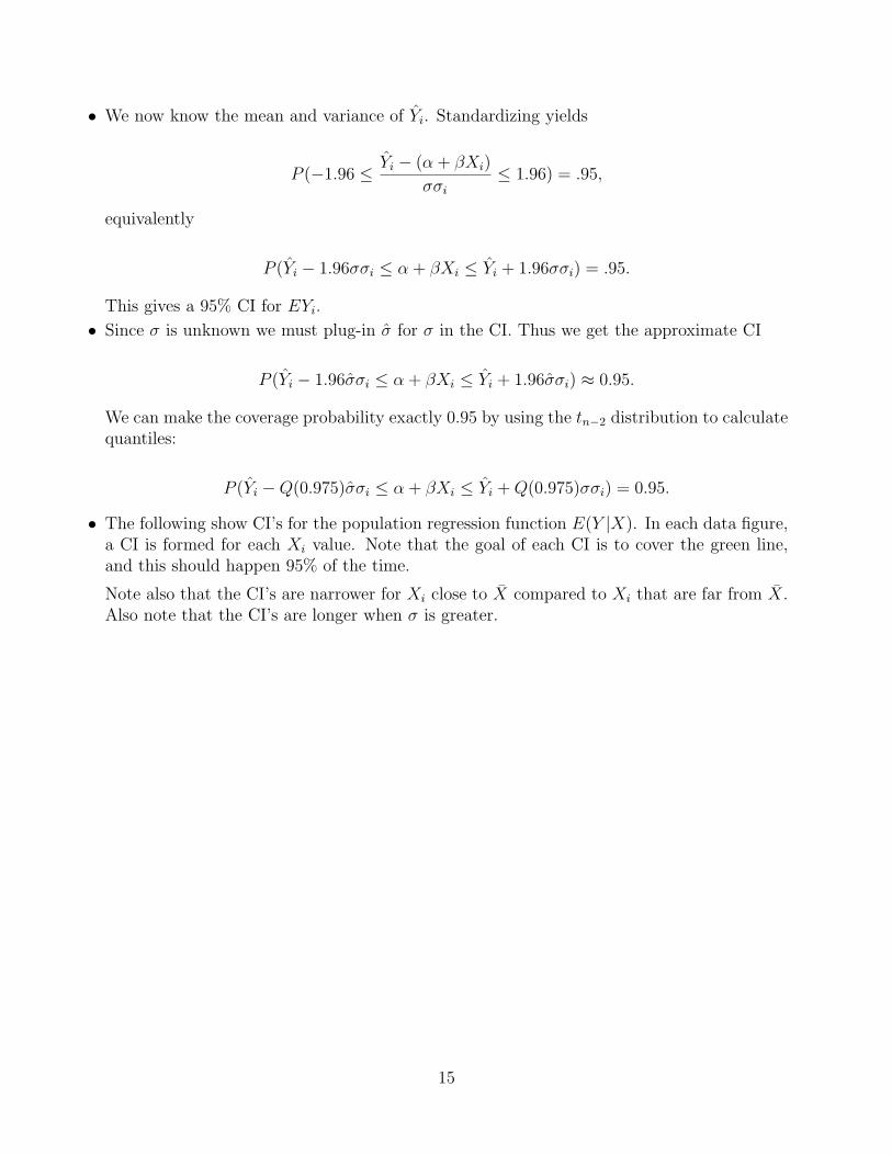
This is an independent realization from the model shown in the previous figure.

-8

-7

-6

-5

-4

-3

-2

-1

0

-1.5 -1 -0.5 0 0.5 1 1.5 2

Another independent realization.

18

Prediction intervals

• Suppose we observe a new X point X∗ after having calculated α and β based on an inde-pendent data set. How can we predict the Y value Y ∗ corresponding to X∗?

It makes sense to use α + βX∗ as the prediction. We would also like to quantify the uncer-tainty in this prediction.

• First note that E(α + βX∗) = α + βX∗ = EY ∗, so the prediction is unbiased.

Calculate the variance of the prediction error:

var(Y ∗ − α− βX∗) = varY ∗ + var(α + βX∗)− 2cov(Y ∗, α + βX∗)

= σ2 + σ2(1 + ((X∗ − X)/σX)2)/n

= σ2(1 + (1 + ((X∗ − X)/σX)2)/n)

= σ2(1 + σ2∗).

Note that the covariance term is 0 since Y ∗ is independent from the data used to fit themodel.When n is large, α and β are very precisely estimated, so σ∗ is very small, and the varianceof the prediction error is ≈ σ2 – nearly all of the uncertainty comes from the error term ε.

The prediction interval

P (−1.96 ≤ Y ∗ − α− βX∗

σ√

1 + σ2∗

≤ 1.96) = .95,

can be rewritten

P (α + βX∗ − 1.96σ√

1 + σ2∗ ≤ Y ∗ ≤ α + βX∗ + 1.96σ

√1 + σ2

∗) = .95.

• As with the CI, we will plug-in σ for σ, making the coverage approximate:

P (α + βX∗ − 1.96σ√

1 + σ2∗ ≤ Y ∗ ≤ α + βX∗ + 1.96σ

√1 + σ2

∗) ≈ .95.

For the coverage probability to be exactly 95%, 1.96 should be replaced with Q(0.975), whereQ is the tn−2 quantile function.

• The following two figures show fitted regression lines for a data set of size n = 20 (the fittedregression line is shown but the data are not shown). Then 95% PI’s are calculated at eachXi, and an independent data set of size n = 20 is generated at the same set of Xi values.The PI’s should cover the new data values 95% of the time.

The PI’s are slightly narrower in the center, but this is hard to see unless n is quite small.

19

-9

-8

-7

-6

-5

-4

-3

-2

-1

0

1

-2 -1.5 -1 -0.5 0 0.5 1 1.5 2

A set of n = 20 bivariate observations were generated according to the modelY = −4+1.4X + ε, where SD(ε) = 1. Based on these points (which are not shown),the fitted regression line (shown in blue) was determined. Next an independentset was generated (black points), with one point having each Xi value from theoriginal data. The vertical blue bars show 95% PI’s at each Xi value.

20

-9

-8

-7

-6

-5

-4

-3

-2

-1

0

1

-1.5 -1 -0.5 0 0.5 1 1.5

An independent replication of the previous figure.

Residuals• The residual ri is the difference between the fitted and observed values at Xi: ri = Yi − Yi.

The residual is a random variable since it depends on the data.

Be sure you understand the difference between the residual (ri) and the error (εi):

Yi = α + βXi + εi

Yi = α + βXi + ri

• Since Eεi = 0, EYi = α + βXi. Thus Eri = EYi − EYi = 0.

Calculate the sum of the residuals:

∑ri =

∑Yi −

∑Yi

=∑

Yi − nα− β∑

Xi.

So the average residual is r = Y − α− βX.

Since α = Y − βX, it follows that r = 0.

21

• Each residual ri estimates the corresponding error εi. The εi are iid, however the ri are notiid.

We already saw that Eri = 0. To calculate varri, begin with:

varri = varYi + varYi − 2cov(Yi, Yi)

= σ2 + σ2σ2i − 2cov(Yi, Yi).

It is a fact that cov(Yi, Yi) = σ2σ2i , thus

varri = σ2 + σ2σ2i − 2σ2σ2

i = σ2(1− σ2i ).

Since a variance must be positive, it must be true that σ2i ≤ 1. This is easier to see by

rewriting σ2i as follows:

σ2i =

1

n+

(Xi − X)2∑j(Xj − X)2

.

It is true that

(Xi − X)2∑j(Xj − X)2

≤ n− 1

n,

but we will not prove this.If the sample size is n = 2, then (X1 − X)2 = (X2 − X)2, so

(Xi − X)2

(X1 − X)2 + (X2 − X)2=

n− 1

n=

1

2,

so the variance of ri is zero in that case.

This makes sense since the regression line fits the data with no residual when there are onlytwo data points.

The residuals ri are less variable than the errors εi since σ2i σ

2 ≤ σ2. Thus the fitted regressionline is closer to the data than the population regression line. This is called overfitting.

Sums of squares

22

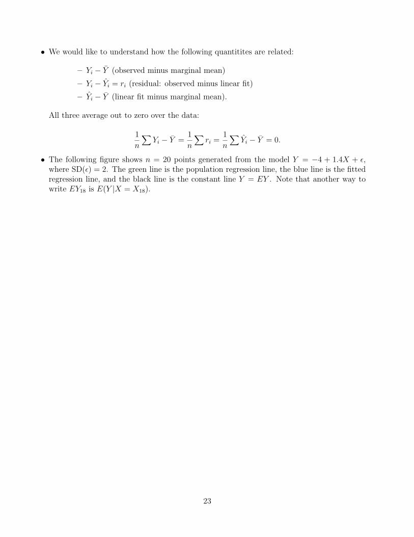
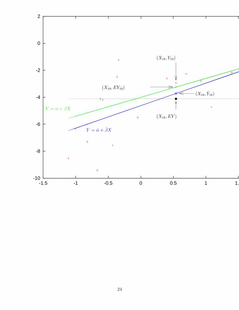
• We would like to understand how the following quantitites are related:

– Yi − Y (observed minus marginal mean)

– Yi − Yi = ri (residual: observed minus linear fit)

– Yi − Y (linear fit minus marginal mean).

All three average out to zero over the data:

1

n

∑Yi − Y =

1

n

∑ri =

1

n

∑Yi − Y = 0.

• The following figure shows n = 20 points generated from the model Y = −4 + 1.4X + ε,where SD(ε) = 2. The green line is the population regression line, the blue line is the fittedregression line, and the black line is the constant line Y = EY . Note that another way towrite EY18 is E(Y |X = X18).

23

-10

-8

-6

-4

-2

0

2

-1.5 -1 -0.5 0 0.5 1 1.5 2

Y = α + βX

Y = α + βX

(X18, EY )

(X18, Y18)

(X18, EY18)

(X18, Y18)

24

• We will begin with two identities. First,

Yi = α + βXi

= Y − βX + βXi

= Y + β(Xi − X).

As a consequence, Yi − Y = β(Xi − X).

Second,

Yi − Yi = Yi − (α + βXi)

= Yi − (Y − βX + βXi)

= Yi − Y − β(Xi − X)

• Now consider the following “sum of squares”:

∑(Yi − Y )2 =

∑(Yi − Yi + Yi − Y )2

=∑

(Yi − Yi)2 +

∑(Yi − Y )2 + 2

∑(Yi − Yi)(Yi − Y ).

Applying the above identities to the final term:

∑(Yi − Yi)(Yi − Y ) = β

∑(Yi − Y − β(Xi − X))(Xi − X)

= β∑

(Yi − Y )(Xi − X)− β(Xi − X)2

= β(n− 1)cov(Y,X)− (n− 1)β2var(X)

= β(n− 1)cov(Y,X)− (n− 1)βcov(Y, X)

= 0

Since the mean of Yi − Yi and the mean of Yi − Y are both zero,

∑(Yi − Yi)(Yi − Y ) = (n− 1)cov(Yi − Yi, Yi − Y ).

Therefore we have shown that the residual ri = Yi − Yi and the fitted values Yi are uncorre-lated.

We now have the following “sum of squares law”:

∑(Yi − Y )2 =

∑(Yi − Yi)

2 +∑

(Yi − Y )2.

25

• The following terminology is used:

Formula Name Abbrev.∑(Yi − Y )2 Total sum of squares SSTO∑(Yi − Yi)

2 Residual sum of squares SSE∑(Yi − Y )2 Regression sum of squares SSR.

The sum of squares law is expressed: “SSTO = SSE + SSR”.

• Corresponding to each “sum of squares” is a “degrees of freedom” (DF). Dividing the sumof squares by the DF gives the “mean square”.

Abbrev. DF Formula

MSTO n-1∑

(Yi − Y )2/(n− 1)

MSE n-2∑

(Yi − Yi)2/(n− 2)

MSR 1∑

(Yi − Y )2

Note that the MSTO is the sample variance, and the MSE is the estimate of σ2 in theregression model.

The “SS” values add: SSTO = SSE + SSR and the degrees of freedom add: n−1 = (n−2)+1.

The “MS” values do not add: MSTO 6= MSE + MSR.

• If the model fits that data well, MSE will be small and MSR will be large. Conversely, if themodel fits the data poorly then MSE will be large and MSR will be small. Thus the statistic

F =MSR

MSE

can be used to evaluate the fit of the linear model (bigger F = better fit).

The distribution of F is an “F distribution with 1, n− 2 DF”, or F1,n−2.

We can test the null hypothesis that the data follow a model Yi = µ+εi against the alternativethat the data follow a model Yi = α+βXi+εi using the F statistic (an “F test”). A computerpackage or a table of the F distribution can be used to determine a p-value.

• In the case of simple linear regression, the F test is equivalent to the hypothesis test β = 0versus β 6= 0. Later when we come to multiple linear regression, this will not be the case.

A useful way to think about what the F-test is evaluating is that the null hypothesis is “allY values have the same expected value” and the alternative is that “the expected value ofYi depends on the value of Xi”.

Diagnostics

26

• In practice, we may not be certain that the assumptions underlying the linear model aresatisfied by a particular data set. To review, the key assumptions are:

1. The conditional mean function E(Y |X) is linear.

2. The conditional variance function var(Y |X) is constant.

3. The errors are normal and independent.

Note that (3) is not essential for the estimates to be valid, but should be approximatelysatisfied for confidence intervals and hypothesis tests to be valid. If the sample size is large,then it is less crucial that (3) be met.

• To assess whether (1) and (2) are satsified, make a scatterplot of the residuals ri against thefitted values Yi.

This is called a “residuals on fitted values plot”.

Recall that we showed above that ri and Yi are uncorrelated.

Thus if the model assumptions are met this plot should look like iid noise – there should beno visually apparent trends or patterns.For example, the following shows how a residual on fitted values plot can be used to detectnonlinearity in the regression function.

-20

-10

0

10

20

30

40

-2 -1.5 -1 -0.5 0 0.5 1 1.5 2

-20

-15

-10

-5

0

5

10

15

20

-10 -5 0 5 10 15 20 25

Res

idua

ls

�

Fitted values

Left: A bivariate data set (red points) with fitted regression line (blue). Right:A diagnostic plot of residuals on fitted values.

27

The following shows how a residual on fitted values plot can be used to detect heteroscedas-ticity.

-6

-5.5

-5

-4.5

-4

-3.5

-3

-2.5

-2

-1.5

-1

-2 -1.5 -1 -0.5 0 0.5 1 1.5 2

-1.5

-1

-0.5

0

0.5

1

1.5

-6 -5.5 -5 -4.5 -4 -3.5 -3 -2.5 -2

Res

idua

ls

�

Fitted values

Left: A bivariate data set (red points) with fitted regression line (blue). Right:A diagnostic plot of residuals on fitted values.

• Suppose that the observations were collected in sequence, say two per day for a period ofone month, yielding n = 60 points. There may be some concern that the distribution hasshifted over time.

These are called “sequence effects” or “time of measurement effects”.

To detect these effects, plot the residual ri against time. There should be no pattern in theplot.

• To assess the normality of the errors use a normal probability plot of the residuals.

For example, the following shows a bivariate data set in which the errors are uniform on[−1, 1] (i.e. any value in that interval is equally likely to occur as the error). This is evidentin the quantile plot of the ri.

28

-7

-6

-5

-4

-3

-2

-1

-2 -1.5 -1 -0.5 0 0.5 1 1.5 2

-2.5

-2

-1.5

-1

-0.5

0

0.5

1

1.5

2

2.5

-2 -1.5 -1 -0.5 0 0.5 1 1.5 2

Nor

mal

Qua

ntile

�

Residual Quantil

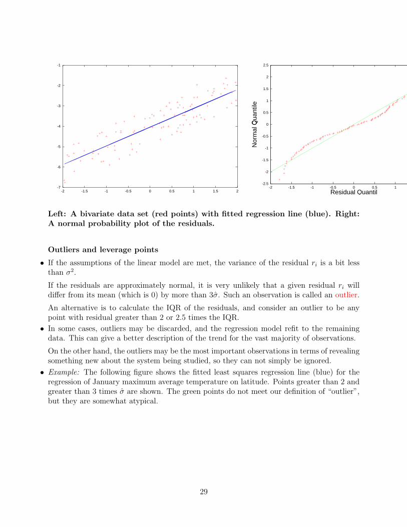
Left: A bivariate data set (red points) with fitted regression line (blue). Right:A normal probability plot of the residuals.

Outliers and leverage points

• If the assumptions of the linear model are met, the variance of the residual ri is a bit lessthan σ2.

If the residuals are approximately normal, it is very unlikely that a given residual ri willdiffer from its mean (which is 0) by more than 3σ. Such an observation is called an outlier.

An alternative is to calculate the IQR of the residuals, and consider an outlier to be anypoint with residual greater than 2 or 2.5 times the IQR.

• In some cases, outliers may be discarded, and the regression model refit to the remainingdata. This can give a better description of the trend for the vast majority of observations.

On the other hand, the outliers may be the most important observations in terms of revealingsomething new about the system being studied, so they can not simply be ignored.

• Example: The following figure shows the fitted least squares regression line (blue) for theregression of January maximum average temperature on latitude. Points greater than 2 andgreater than 3 times σ are shown. The green points do not meet our definition of “outlier”,but they are somewhat atypical.

29

10

20

30

40

50

60

70

80

20 25 30 35 40 45 50

Janu

ary

Tem

pera

ture

�

Latitude

Non outliers2 SD outliers3 SD outliers

Ann Arbor, MI

It turns out that of the 19 outliers, 18 are warmer than expected, and these stations are allin northern California and Oregon.

The one outlier station that is substantially colder than expected is in Gunnison County,Colorado, which is very high in elevation (at 2,339 ft, it is the fourth highest of 1072 stationsin the data set).

In January 2001, Ann Arbor, Michigan was slightly colder than the fitted value (i.e. it wasa bit colder here than in other places of similar latitude).

30

-25

-20

-15

-10

-5

0

5

10

15

20

25

30

20 30 40 50 60 70 80

Res

idua

ls

Fitted values

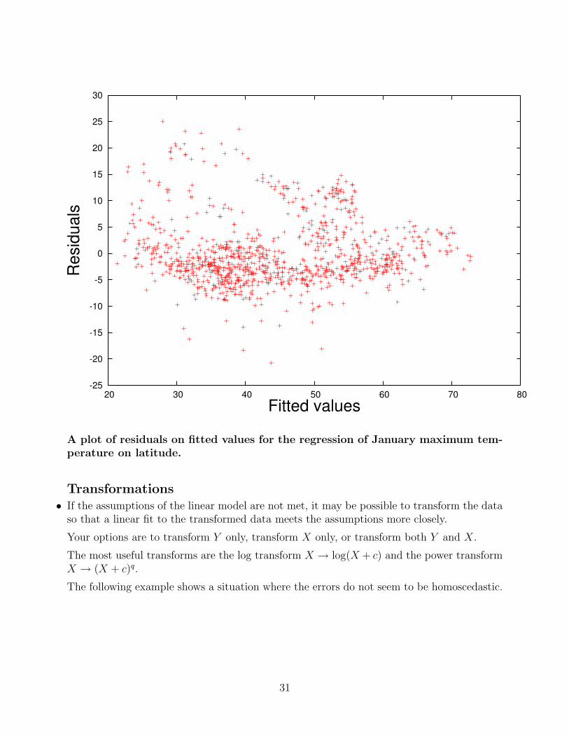
A plot of residuals on fitted values for the regression of January maximum tem-perature on latitude.

Transformations• If the assumptions of the linear model are not met, it may be possible to transform the data

so that a linear fit to the transformed data meets the assumptions more closely.

Your options are to transform Y only, transform X only, or transform both Y and X.

The most useful transforms are the log transform X → log(X + c) and the power transformX → (X + c)q.

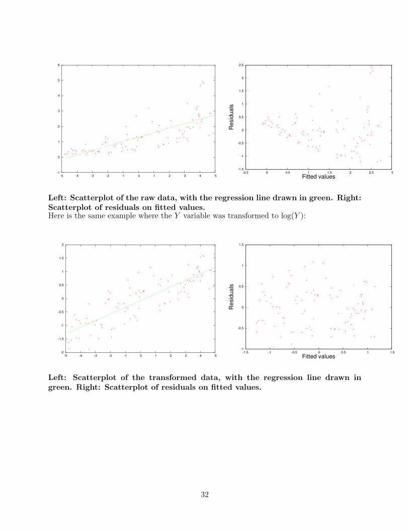
The following example shows a situation where the errors do not seem to be homoscedastic.

31

-1

0

1

2

3

4

5

6

-5 -4 -3 -2 -1 0 1 2 3 4 5

-1.5

-1

-0.5

0

0.5

1

1.5

2

2.5

-0.5 0 0.5 1 1.5 2 2.5 3

Res

idua

ls

Fitted values

Left: Scatterplot of the raw data, with the regression line drawn in green. Right:Scatterplot of residuals on fitted values.Here is the same example where the Y variable was transformed to log(Y ):

-2

-1.5

-1

-0.5

0

0.5

1

1.5

2

-5 -4 -3 -2 -1 0 1 2 3 4 5

-1

-0.5

0

0.5

1

1.5

-1.5 -1 -0.5 0 0.5 1 1.5

Res

idua

ls

Fitted values

Left: Scatterplot of the transformed data, with the regression line drawn ingreen. Right: Scatterplot of residuals on fitted values.

32

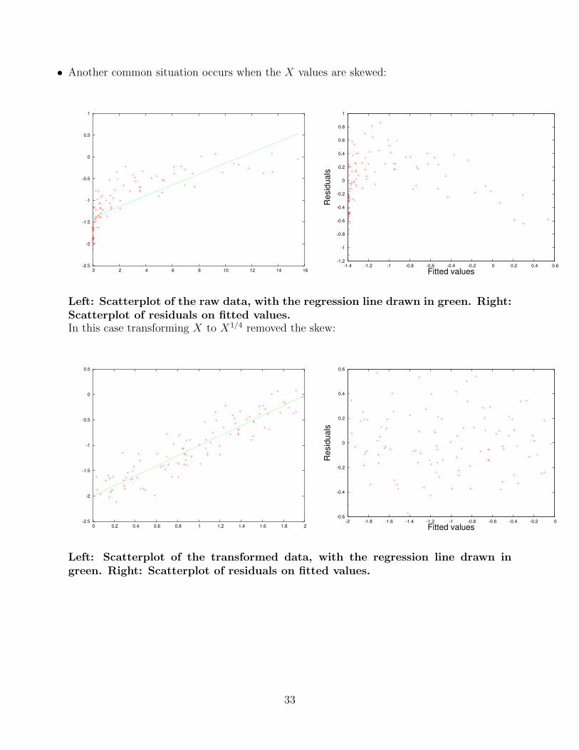
• Another common situation occurs when the X values are skewed:

-2.5

-2

-1.5

-1

-0.5

0

0.5

1

0 2 4 6 8 10 12 14 16

-1.2

-1

-0.8

-0.6

-0.4

-0.2

0

0.2

0.4

0.6

0.8

1

-1.4 -1.2 -1 -0.8 -0.6 -0.4 -0.2 0 0.2 0.4 0.6

Res

idua

ls

Fitted values

Left: Scatterplot of the raw data, with the regression line drawn in green. Right:Scatterplot of residuals on fitted values.In this case transforming X to X1/4 removed the skew:

-2.5

-2

-1.5

-1

-0.5

0

0.5

0 0.2 0.4 0.6 0.8 1 1.2 1.4 1.6 1.8 2

-0.6

-0.4

-0.2

0

0.2

0.4

0.6

-2 -1.8 -1.6 -1.4 -1.2 -1 -0.8 -0.6 -0.4 -0.2 0

Res

idua

ls

Fitted values

Left: Scatterplot of the transformed data, with the regression line drawn ingreen. Right: Scatterplot of residuals on fitted values.

33

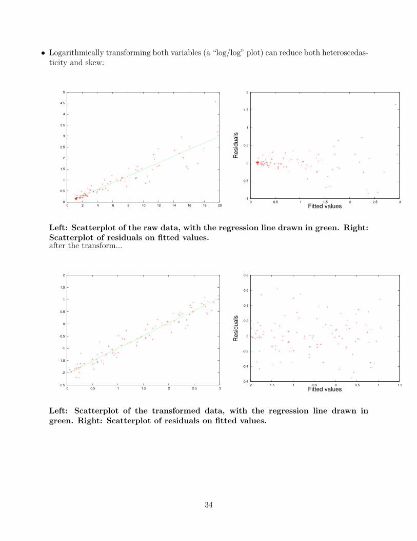
• Logarithmically transforming both variables (a “log/log” plot) can reduce both heteroscedas-ticity and skew:

0

0.5

1

1.5

2

2.5

3

3.5

4

4.5

5

0 2 4 6 8 10 12 14 16 18 20

-1

-0.5

0

0.5

1

1.5

2

0 0.5 1 1.5 2 2.5 3

Res

idua

ls

Fitted values

Left: Scatterplot of the raw data, with the regression line drawn in green. Right:Scatterplot of residuals on fitted values.after the transform...

-2.5

-2

-1.5

-1

-0.5

0

0.5

1

1.5

2

0 0.5 1 1.5 2 2.5 3

-0.6

-0.4

-0.2

0

0.2

0.4

0.6

0.8

-2 -1.5 -1 -0.5 0 0.5 1 1.5

Res

idua

ls

Fitted values

Left: Scatterplot of the transformed data, with the regression line drawn ingreen. Right: Scatterplot of residuals on fitted values.

34