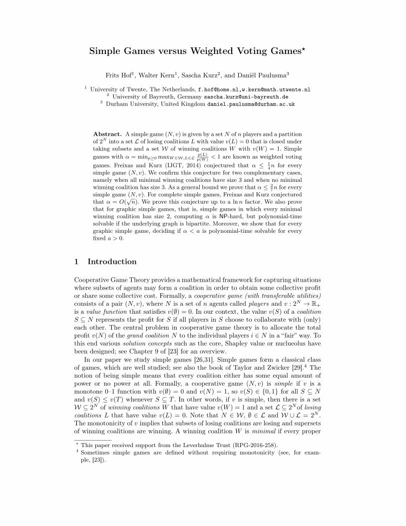
Simple Games versus Weighted Voting Games?

Frits Hof1, Walter Kern1, Sascha Kurz2, and Daniël Paulusma3

1 University of Twente, The Netherlands, f.hof@home.nl,w.kern@math.utwente.nl2 University of Bayreuth, Germany sascha.kurz@uni-bayreuth.de

3 Durham University, United Kingdom daniel.paulusma@durham.ac.uk

Abstract. A simple game (N, v) is given by a setN of n players and a partitionof 2N into a set L of losing coalitions L with value v(L) = 0 that is closed undertaking subsets and a set W of winning coalitions W with v(W ) = 1. Simplegames with α = minp≥0 maxW∈W,L∈L

p(L)p(W )

< 1 are known as weighted votinggames. Freixas and Kurz (IJGT, 2014) conjectured that α ≤ 1

4n for every

simple game (N, v). We confirm this conjecture for two complementary cases,namely when all minimal winning coalitions have size 3 and when no minimalwinning coalition has size 3. As a general bound we prove that α ≤ 2

7n for every

simple game (N, v). For complete simple games, Freixas and Kurz conjecturedthat α = O(

√n). We prove this conjecture up to a lnn factor. We also prove

that for graphic simple games, that is, simple games in which every minimalwinning coalition has size 2, computing α is NP-hard, but polynomial-timesolvable if the underlying graph is bipartite. Moreover, we show that for everygraphic simple game, deciding if α < a is polynomial-time solvable for everyfixed a > 0.

1 Introduction

Cooperative Game Theory provides a mathematical framework for capturing situationswhere subsets of agents may form a coalition in order to obtain some collective profitor share some collective cost. Formally, a cooperative game (with transferable utilities)consists of a pair (N, v), where N is a set of n agents called players and v : 2N → R+

is a value function that satisfies v(∅) = 0. In our context, the value v(S) of a coalitionS ⊆ N represents the profit for S if all players in S choose to collaborate with (only)each other. The central problem in cooperative game theory is to allocate the totalprofit v(N) of the grand coalition N to the individual players i ∈ N in a “fair” way. Tothis end various solution concepts such as the core, Shapley value or nuclueolus havebeen designed; see Chapter 9 of [23] for an overview.

In our paper we study simple games [26,31]. Simple games form a classical classof games, which are well studied; see also the book of Taylor and Zwicker [29].4 Thenotion of being simple means that every coalition either has some equal amount ofpower or no power at all. Formally, a cooperative game (N, v) is simple if v is amonotone 0–1 function with v(∅) = 0 and v(N) = 1, so v(S) ∈ 0, 1 for all S ⊆ Nand v(S) ≤ v(T ) whenever S ⊆ T . In other words, if v is simple, then there is a setW ⊆ 2N of winning coalitions W that have value v(W ) = 1 and a set L ⊆ 2Nof losingcoalitions L that have value v(L) = 0. Note that N ∈ W, ∅ ∈ L and W ∪ L = 2N .The monotonicity of v implies that subsets of losing coalitions are losing and supersetsof winning coalitions are winning. A winning coalition W is minimal if every proper

? This paper received support from the Leverhulme Trust (RPG-2016-258).4 Sometimes simple games are defined without requiring monotonicity (see, for exam-ple, [23]).

subset of W is losing, and a losing coalition L is maximal if every proper superset ofL is winning.

A simple game is a weighted voting game if there exists a payoff vector p ∈ Rn+such that a coalition S is winning if p(S) ≥ 1 and losing if p(S) < 1. Weighted votinggames are also known as weighted majority games and form one of the most pop-ular classes of simple games. Due to their practical applications in voting systems,computer operating systems and model resource allocation (see e.g. [2,6]), structuraland computational complexity aspects for solution concepts for weighted voting gameshave been thoroughly investigated [8,9,12,15]. However, it is easy to construct simplegames that are not weighted voting games. We give an example below, but in factthere are many important simple games that are not weighted voting games, and therelationship between weighted voting games and simple games is not yet fully under-stood. Therefore, Gvozdeva, Hemaspaandra, and Slinko [15] introduced a parameterα, called the critical threshold value, to measure the “distance” of a simple game tothe class of weighted voting games:

α = α(N, v) = minp≥0

maxW,L

p(L)

p(W ), (1)

where the maximum is taken over all winning coalitions in W and all losing coalitionsin L. A simple game (N, v) is a weighted voting game if and only if α < 1.5 This followsfrom observing that each optimal solution p of (1) can be scaled to satisfy p(W ) ≥ 1for all winning coalitions W .

A concrete example of a simple game (N, v) that is not a weighted voting game andthat has in fact a large value of α was given in [11]. Let N = 1, . . . , n for some eveninteger n ≥ 4, and let the minimal winning coalitions be the pairs 1, 2, 2, 3, . . . n−1, n, n, 1. Consider any payoff p ≥ 0 satisfying p(W ) ≥ 1 for every winning coali-tion W . Then pi + pi+1 ≥ 1 for i = 1, . . . , n (where n + 1 = 1). This means thatp(N) ≥ 1

2n. Then, for at least one of L = 2, 4, 6, . . . , n and L = 1, 3, 5, . . . , n− 1,we have p(L) ≥ 1

4n, showing that α ≥ 14n. On the other hand, it is easily seen that

p ≡ 12 satisfies p(W ) ≥ 1 for all winning coalitions and p(L) ≤ 1

4n for all losing coali-tions, showing that α ≤ 1

4n. Thus we conclude that α = 14n. Due to this somewhat

extreme example, the authors of [11] conjectured that α ≤ 14n for all simple games.

This conjecture turns out to be an interesting combinatorial problem.Conjecture 1 [11]. For every simple game (N, v), it holds that α ≤ 1

4n.

1.1 Our Results

In Section 2 we prove that Conjecture 1 holds for the case where all minimal winningcoalitions have size 3 and for its complementary case where no minimal winning collec-tion has size 3. We were not able to prove Conjecture 1 for all simple games. However,in Section 3 we show that α ≤ 2

7n ≈ 0.2858n for every simple game.In Section 4 we consider a subclass of simple games based on a natural desirability

order [24]. A simple game (N, v) is complete if the players can be ordered by a complete,transitive ordering , say, 1 2 · · · n, indicating that higher ranked players havemore power (and are more desirable) than lower ranked players. More precisely, i jmeans that v(S ∪ i) ≥ v(S ∪ j) for any coalition S ⊆ N\i, j. The class ofcomplete simple games properly contains all weighted voting games [13]. For completesimple games, we show a lower bound on α that is asymptotically lower than 1

4n,namely α = O(

√n lnn). This bound matches, up to a lnn factor, the lower bound of

Ω(√n) in [11] (conjectured to be tight in [11]).

5 If α ≤ 1, we speak of roughly weighted voting games [29].

2

In Section 5 we discuss some algorithmic and complexity issues. We focus on in-stances where all minimal winning coalitions have size 2. We say that such simplegames are graphic, as they can conveniently be described by a graph G = (N,E) withvertex set N and edge set E = ij | i, j is winning. For graphic simple gameswe show that computing α is NP-hard in general (see below for some related results).On the positive side, we show that computing α is polynomial-time solvable if theunderlying graph G = (N,E) is bipartite, or if α is known to be small (less than afixed number a). We conclude with some remarks and open problems in Section 6.

1.2 Related Work

Another way to measure the distance of a simple game to the class of weighted votinggames is to use the dimension of a simple game [28], which is the smallest numberof weighted voting games whose intersection equals a given simple game. However,computing the dimension of a simple game is NP-hard [7], and the largest dimension ofa simple game with n players is 2n−o(n) [20]. Moreover, simple games with dimension 1have α = 1, but α may be arbitrarily large for simple games with dimension largerthan 1.6 Hence there is no direct relation between the two distance measures. We alsonote that Gvozdeva, Hemaspaandra, and Slinko [15] introduced two other distanceparameters. One measures the power balance between small and large coalitions. Theother one allows multiple thresholds instead of threshold 1 only. See [15] for furtherdetails.

For graphic simple games, it is natural to take the number of players n as theinput size for answering complexity questions, but in general simple games may havedifferent representations. For instance, one can list all minimal winning coalitions orall maximal losing coalitions. Under these two representations the problem of decidingif α < 1, that is, if a given simple game is a weighted voting game, is also polynomial-time solvable. This follows from results of Hegedüs and Megiddo [16] and Peled andSimeone [22], as shown by Freixas, Molinero, Olsen and Serna [12]. The latter authorsalso showed that the same result holds if the representation is given by listing allwinning coalitions or all losing coalitions. Moreover, they gave a number of complexityresults of recognizing other subclasses of simple games.

We also note a similarity of our research with research into matching games. InSection 2 we show that a crucial case in our study is when the simple game is graphic,that is, defined on some graph G = (N,E). In the corresponding matching game acoalition S ⊆ N has value v(S) equal to the maximum size of a matching in thesubgraph of G induced by S. One of the most prominent solution concepts is the coreof a game, defined by core(N, v) := p ∈ Rn | p(N) = v(N), p(S) ≥ v(S) ∀S ⊆ N.A core allocation is stable, as no coalition has any incentive to object against it.However, the core may be empty. Matching games are not simple games. Yet their coreconstraints are readily seen to simplify to p ≥ 0 and pi+pj ≥ 1 for all ij ∈ E. Classicalsolution concepts, such as the core and core-related ones like least core, nucleolusor nucleon are well studied for matching games, see, for example, [3,4,10,18,19,27].However, the problems encountered there differ with respect to the objective function.For graphic simple games we aim to bound p(L) over all losing coalitions, subject top ≥ 0, pi + pj ≥ 1 for all ij ∈ E, whereas for matching games with an empty corewe wish to bound p(N), subject to p ≥ 0, pi + pj ≥ 1 for all ij ∈ E. Nevertheless,basic tools from matching theory like the Gallai-Edmonds decomposition play a rolein both cases.6 A simple game with 1

2n players of type A and 1

2n players of type B and minimal winning

coalitions consisting of one player of each type has dimension 2 and α = 14n.

3

2 Two Complementary Cases

In this section we will consider the following two “complementary” cases: when allwinning coalitions have size equal to 3 (Section 2.1), and when no winning coalitionhas size equal to 3 (Section 2.2). First observe that winning coalitions of size 1 donot cause any problems. If i is a winning coalition of size 1, we satisfy it by settingpi = 1. Since no losing coalition L contains i, we may remove i from the game andsolve (1) with respect to the resulting subgame. A similar argument applies if somei ∈ N is not contained in any minimal winning coalition. We then simply define pi = 0and remove i from the game. Thus, we may assume without loss of generality that allminimal winning coalitions have size at least 2 and that they cover all of N .

2.1 All Minimal Winning Coalitions Have Size 2.

We first investigate the case where all minimal winning coalitions have size exactly 2.This case (which is a crucial case in our study) can conveniently be translated toa graph-theoretic problem. Let G = (N,E) be the graph with vertex set N whoseedges are exactly the minimal winning coalitions of size 2 in our game (N, v). Ourassumption that N is completely covered by minimal winning coalitions means that Ghas no isolated vertices. Losing coalitions correspond to independent sets of verticesL ⊆ N . Then the min max problem (1) becomes

α := αG := minp

maxL

p(L), (2)

where the minimum is taken over all feasible pay-off vectors p, that is, p ∈ Rn+ withpi + pj ≥ 1 for every ij ∈ E, and the maximum is taken over all independent setsL ⊆ N .

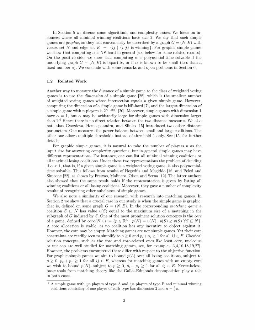
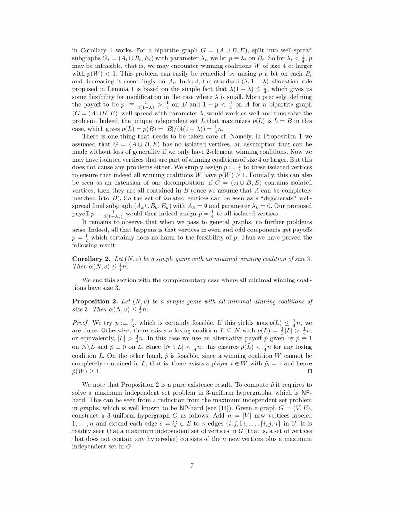
We first consider the case where G = (A ∪B,E) is bipartite. To explain the basicidea, we introduce the following concept (illustrated in Figure 1).

A S

B N(S)

Fig. 1. A well-spread bipartite graph.

Definition. Let G = (A ∪ B,E) be a bipartite graph of order n = |A|+ |B| withoutisolated notes and assume without loss of generality that |A| ≤ |B|. Let λ ≤ 1

2 suchthat |A| = λn (and |B| = (1− λ)n). We say that G is well-spread with parameter λ iffor all S ⊆ A we have

|S||N(S)|

≤ |A||B|

=λ

1− λ.

(Here, as usual, N(S) ⊆ B denotes the set of neighbors of S in B.)Examples of well-spread bipartite graphs are biregular graphs or biregular graphsminus an edge. Note that if G is well-spread with parameter λ ≤ 1

2 , then Hall’scondition |N(S)| ≥ |S| for all S ⊆ A is satisfied, implying that A can be completelymatched to B (see, for example, [21]). The following lemma is the key observation.

4

Lemma 1. Let G = (A ∪B,E) be well-spread with parameter λ ≤ 12 . Then p ≡ λ on

B and p ≡ 1− λ on A yields αG ≤ 14n.

Proof. Assume L ⊆ N is an independent set. Let ρ ≤ 1 such that |L∩A| = ρλn. SinceG is well-spread, we get |N(L ∩ A)| ≥ ρ(1 − λ)n, so that |L ∩ B| ≤ (1 − ρ)(1 − λ)n.Thus

p(L) = |L ∩A|(1− λ) + |L ∩B|λ≤ ρλn(1− λ) + (1− ρ)(1− λ)nλ

≤ ρ 14n+ (1− ρ) 1

4n

≤ 14n.

Hence we have proven the lemma. ut

In general, when G = (A ∪B,E) is not well-spread, we seek to decompose G intowell-spread induced subgraphs Gi = (Ai ∪ Bi, Ei) with A =

⋃Ai and B =

⋃Bi. Of

course, this can only work if G = (A∪B,E) is such that A can be matched to B in G.

Proposition 1. Let G = (A∪B,E) be a bipartite graph without isolated vertices andassume that A can be matched into B. Then G decomposes into well-spread inducedsubgraphs Gi = (Ai ∪Bi, Ei), with A =

⋃Ai and B =

⋃Bi in such a way that for all

i, j with i < j, λi ≥ λj and no edges join Ai to Bj. ut

Proof. Let S ⊆ A maximize |S|/|N(S). Set A1 := S and B1 := N(S). Let G′ be thesubgraph of G induced by A\A1 and B′ := B\B1. Then G′ satisfies the assumptionof the Proposition. Indeed, if A′ cannot be matched into B′ in G′, then there must besome S′ ⊆ A′ with |S′| > |N ′(S′)|, where N ′(S′) = N(S′)\B1 is the neighborhood ofS′ in G′. But then |S ∪S′| = |S|+ |S′| and |N(S ∪S′)| ≤ |N(S)|+ |N ′(S)| shows thatS cannot maximize |S|/|N(S)|, a contradiction. Thus, by induction, we may assumethat G′ decomposes in the desired way into well-spread subgraphs G2, . . . , Gk withparameters λ2 ≥ · · · ≥ λk. The claim then follows by observing that (i) no edgesjoin B1 to A′; and (ii) λ1 ≥ λ2 (otherwise S ∪ A2 would contradict the choice of Smaximizing |S|/|N(S)|). ut

We now combining the last two results.

Corollary 1. For every bipartite graph G = (A ∪ B,E) of order n satisfying theassumption of Proposition 1, there exists a payoff vector p ≥ 0 such that pi + pj ≥ 1for ij ∈ E and p(L) ≤ 1

4n for any independent set L ⊆ A ∪ B. In addition, p can bechosen so as to satisfy p ≥ 1

2 on A.

Proof. The result follow immediately from Lemma 1 and Proposition 1. Note that ifp is chosen as p ≡ 1− λi on Ai, then p ≥ 1

2 indeed. ut

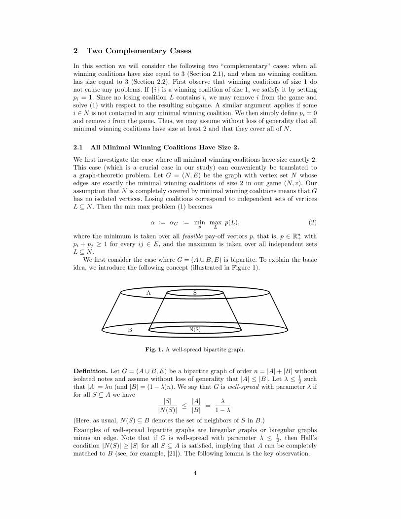
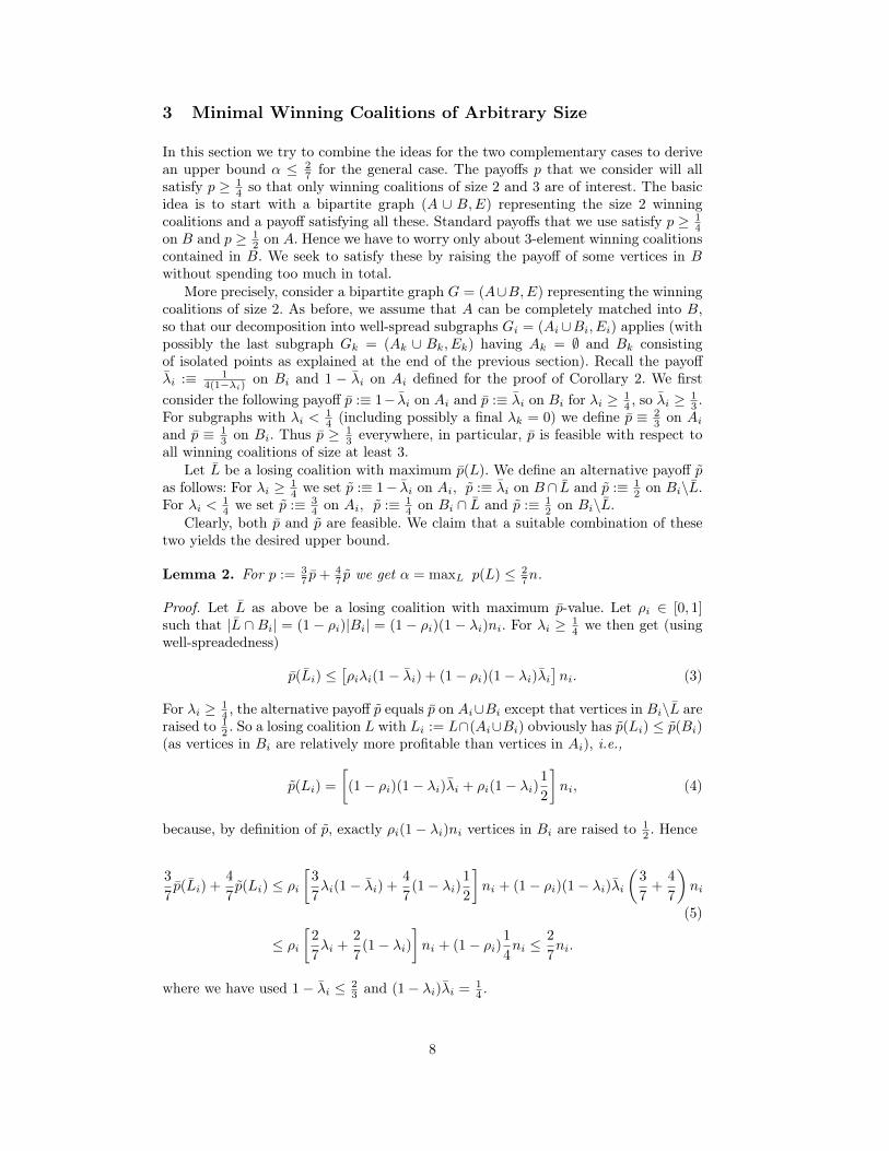
As we will see, the assumption of Proposition 1 is not really restrictive for ourpurposes. A (connected) component C of a graph G is even (odd) if C has an even(odd) number of vertices. A graph G = (N,E) is factor-critical if for every vertexv ∈ V (G), the graph G− v has a perfect matching. We recall the well-known Gallai–Edmonds Theorem (see [21]) for characterizing the structure of maximum matchingsin G; see also Figure 2. There exists a (unique) subset A ⊆ N , called a Tutte set, suchthat

– every even component of G−A has a perfect matching;– every odd component of G−A is factor-critical;– every maximum matching in G is the union of a perfect matching in each even

component, a nearly perfect matching in each odd component and a matching thatmatches A (completely) to the odd components.

5

A

even

odd

Fig. 2. Tutte set A splitting G into even and odd components (possibly single nodes).

We are now ready to derive our first main result.7

Theorem 1. Let G = (N,E) be a graph of order n. Then αG ≤ 14n.

Proof. Let A ⊆ N be a Tutte set. Contract each odd component in G−A to a singlevertex and let B denote the resulting set of vertices. The subgraph G induced by A∪Bthen satisfies the assumption of Corollary 1. Let p ∈ R|A|+|B| be the correspondingpayoff vector. We define p ∈ Rn by setting pi = pi for every vertex i ∈ A and everyvertex i that corresponds to an odd component of size 1 in G − A. All other verticesget pj = 1

2 .It is straightforward to check that p ≥ 0 and pi+pj ≥ 1. Indeed, p ≥ 1

2 everywhereexcept on B, so the only critical edges ij have i ∈ A and j a singleton odd component.But in this case pi + pj = pi + pj ≥ 1. Thus we are left to prove that for everyindependent set L ⊆ N , p(L) ≤ 1

4n. Let B0 denote the set of singleton odd componentsi ∈ B, L0 := (L∩A)∪ (L∩B0) and n0 := |A|+ |B|. Clearly, L0 is an independent setin the bipartite graph G , and p = p on L0. We thus conclude that p(L0) ≤ 1

4n0.Next let us analyze L ∩ C where C ⊆ N\A is an even component. C is perfectly

matchable, implying that L contains at most |C|/2 vertices of C. So p(L∩C) ≤ 14 |C|.

A similar argument applies to odd components. Let C be an odd component in G−Aof size at least 3. Then certainly L cannot contain all vertices of C, so there existssome i ∈ C\L. Since C is factor-critical, C\i is perfectly matchable, implying that Lcan contain at most half of C\i. Thus |L∩C| ≤ (|C|−1)/2 and p(L∩C) ≤ (|C|−1)/4.

Summarizing, n−n0 = |N |− (|A|+ |B|) is the sum over all |C|, where C is an evencomponent plus the sum over all |C| − 1 where C is an odd component, and p(L\L0)is at most a 1

4 fraction of this, finishing the proof. ut

We like to mention that both decompositions that we use to define the payoff pcan be computed efficiently. For the Edmonds–Gallai decomposition, this is a well-known fact (see, for example, [21]). For the decomposition into well-spread subgraphs,this follows from the observation that deciding whether maxS

|S||N(S)| ≤ r is equivalent

to minS r|N(S)| − |S| ≥ 0, which amounts to minimizing the submodular functionf(S) = r|N(S)| − |S|; see, for example, [25] for a strongly polynomial-time algorithmor Appendix A.

2.2 No Minimal Winning Sets of Size 3

We now deal shortly with the more general case where there are, in addition, minimalwinning coalitions of size 4 or larger. First recall how the payoff p that we proposed

7 For n is odd, the upper bound in Theorem 1 can be slightly strengthened to n2−14n

[17].

6

in Corollary 1 works. For a bipartite graph G = (A ∪ B,E), split into well-spreadsubgraphs Gi = (Ai ∪Bi, Ei) with parameter λi, we let p ≡ λi on Bi. So for λi < 1

4 , pmay be infeasible, that is, we may encounter winning coalitions W of size 4 or largerwith p(W ) < 1. This problem can easily be remedied by raising p a bit on each Biand decreasing it accordingly on Ai. Indeed, the standard (λ, 1 − λ) allocation ruleproposed in Lemma 1 is based on the simple fact that λ(1 − λ) ≤ 1

4 , which gives ussome flexibility for modification in the case where λ is small. More precisely, definingthe payoff to be p :≡ 1

4(1−λ) >14 on B and 1 − p < 3

4 on A for a bipartite graph(G = (A∪B,E), well-spread with parameter λ, would work as well and thus solve theproblem. Indeed, the unique independent set L that maximizes p(L) is L = B in thiscase, which gives p(L) = p(B) = |B|/(4(1− λ)) = 1

4n.There is one thing that needs to be taken care of. Namely, in Proposition 1 we

assumed that G = (A ∪ B,E) has no isolated vertices, an assumption that can bemade without loss of generality if we only have 2-element winning coalitions. Now wemay have isolated vertices that are part of winning coalitions of size 4 or larger. But thisdoes not cause any problems either. We simply assign p := 1

4 to these isolated verticesto ensure that indeed all winning coalitions W have p(W ) ≥ 1. Formally, this can alsobe seen as an extension of our decomposition: if G = (A ∪ B,E) contains isolatedvertices, then they are all contained in B (once we assume that A can be completelymatched into B). So the set of isolated vertices can be seen as a “degenerate” well-spread final subgraph (Ak∪Bk, Ek) with Ak = ∅ and parameter λk = 0. Our proposedpayoff p ≡ 1

4(1−λk)would then indeed assign p = 1

4 to all isolated vertices.It remains to observe that when we pass to general graphs, no further problems

arise. Indeed, all that happens is that vertices in even and odd components get payoffsp = 1

2 which certainly does no harm to the feasibility of p. Thus we have proved thefollowing result.

Corollary 2. Let (N, v) be a simple game with no minimal winning coalition of size 3.Then α(N, v) ≤ 1

4n.

We end this section with the complementary case where all minimal winning coali-tions have size 3.

Proposition 2. Let (N, v) be a simple game with all minimal winning coalitions ofsize 3. Then α(N, v) ≤ 1

4n.

Proof. We try p :≡ 13 , which is certainly feasible. If this yields max p(L) ≤ 1

4n, weare done. Otherwise, there exists a losing coalition L ⊆ N with p(L) = 1

3 |L| >14n,

or equivalently, |L| > 34n. In this case we use an alternative payoff p given by p ≡ 1

on N\L and p ≡ 0 on L. Since |N \ L| < 14n, this ensures p(L) < 1

4n for any losingcoalition L. On the other hand, p is feasible, since a winning coalition W cannot becompletely contained in L, that is, there exists a player i ∈W with pi = 1 and hencep(W ) ≥ 1. ut

We note that Proposition 2 is a pure existence result. To compute p it requires tosolve a maximum independent set problem in 3-uniform hypergraphs, which is NP-hard. This can be seen from a reduction from the maximum independent set problemin graphs, which is well known to be NP-hard (see [14]). Given a graph G = (V,E),construct a 3-uniform hypergraph G as follows. Add n = |V | new vertices labeled1, . . . , n and extend each edge e = ij ∈ E to n edges i, j, 1, . . . , i, j, n in G. It isreadily seen that a maximum independent set of vertices in G (that is, a set of verticesthat does not contain any hyperedge) consists of the n new vertices plus a maximumindependent set in G.

7

3 Minimal Winning Coalitions of Arbitrary Size

In this section we try to combine the ideas for the two complementary cases to derivean upper bound α ≤ 2

7 for the general case. The payoffs p that we consider will allsatisfy p ≥ 1

4 so that only winning coalitions of size 2 and 3 are of interest. The basicidea is to start with a bipartite graph (A ∪ B,E) representing the size 2 winningcoalitions and a payoff satisfying all these. Standard payoffs that we use satisfy p ≥ 1

4on B and p ≥ 1

2 on A. Hence we have to worry only about 3-element winning coalitionscontained in B. We seek to satisfy these by raising the payoff of some vertices in Bwithout spending too much in total.

More precisely, consider a bipartite graph G = (A∪B,E) representing the winningcoalitions of size 2. As before, we assume that A can be completely matched into B,so that our decomposition into well-spread subgraphs Gi = (Ai∪Bi, Ei) applies (withpossibly the last subgraph Gk = (Ak ∪ Bk, Ek) having Ak = ∅ and Bk consistingof isolated points as explained at the end of the previous section). Recall the payoffλi :≡ 1

4(1−λi)on Bi and 1 − λi on Ai defined for the proof of Corollary 2. We first

consider the following payoff p :≡ 1− λi on Ai and p :≡ λi on Bi for λi ≥ 14 , so λi ≥

13 .

For subgraphs with λi < 14 (including possibly a final λk = 0) we define p ≡ 2

3 on Aiand p ≡ 1

3 on Bi. Thus p ≥ 13 everywhere, in particular, p is feasible with respect to

all winning coalitions of size at least 3.Let L be a losing coalition with maximum p(L). We define an alternative payoff p

as follows: For λi ≥ 14 we set p :≡ 1− λi on Ai, p :≡ λi on B ∩ L and p :≡ 1

2 on Bi\L.For λi < 1

4 we set p :≡ 34 on Ai, p :≡ 1

4 on Bi ∩ L and p :≡ 12 on Bi\L.

Clearly, both p and p are feasible. We claim that a suitable combination of thesetwo yields the desired upper bound.

Lemma 2. For p := 37 p+ 4

7 p we get α = maxL p(L) ≤ 27n.

Proof. Let L as above be a losing coalition with maximum p-value. Let ρi ∈ [0, 1]such that |L ∩ Bi| = (1− ρi)|Bi| = (1− ρi)(1− λi)ni. For λi ≥ 1

4 we then get (usingwell-spreadedness)

p(Li) ≤[ρiλi(1− λi) + (1− ρi)(1− λi)λi

]ni. (3)

For λi ≥ 14 , the alternative payoff p equals p on Ai∪Bi except that vertices in Bi\L are

raised to 12 . So a losing coalition L with Li := L∩(Ai∪Bi) obviously has p(Li) ≤ p(Bi)

(as vertices in Bi are relatively more profitable than vertices in Ai), i.e.,

p(Li) =

[(1− ρi)(1− λi)λi + ρi(1− λi)

1

2

]ni, (4)

because, by definition of p, exactly ρi(1− λi)ni vertices in Bi are raised to 12 . Hence

3

7p(Li) +

4

7p(Li) ≤ ρi

[3

7λi(1− λi) +

4

7(1− λi)

1

2

]ni + (1− ρi)(1− λi)λi

(3

7+

4

7

)ni

(5)

≤ ρi[

2

7λi +

2

7(1− λi)

]ni + (1− ρi)

1

4ni ≤

2

7ni.

where we have used 1− λi ≤ 23 and (1− λi)λi = 1

4 .

8

For λi < 14 (i.e., λi < 1

3 ), we conclude similarly that

p(Li) ≤[ρiλi

2

3+ (1− ρi)(1− λi)

1

3

]ni (6)

andp(Li) =

[(1− ρi)(1− λi)

1

4+ ρi(1− λi)

1

2

]ni. (7)

Thus,

3

7p(Li) +

4

7p(Li) ≤

[ρi

(2

7λi +

2

7(1− λi)

)+ (1− ρi)(1− λi)

(1

7+

1

7

)]ni (8)

≤[ρi

2

7+ (1− ρi)

2

7

]ni =

2

7ni. (9)

Now the claim follows by observing that p(L) = 37 p(L) + 4

7 p(L) ≤ 37 p(L) + 4

7 p(L). ut

Hence we obtained the following theorem.

Theorem 2. For every simple game (N, v), α(N, v) ≤ 27n.

4 Complete Simple Games

Recall that a simple game (N, v) is complete if for a suitable ordering, say, 1 2 · · · n indicating that i is more powerful than i + 1 in the sense that v(S ∪ i) ≥v(S ∪ i+ 1) for any coalition S ⊆ N\i, j. Intuitively, the class of complete simplegames is “closer” to weighted voting games than general simple games. The next resultquantifies this expectation.

Theorem 3. A complete simple game (N, v) has α ≤√n lnn.

Proof. Let N = 1, . . . , n be the set of players and assume without loss of generalitythat 1 2 · · · n. Let k ∈ N be the largest number such that k, . . . , n is winning.For i = 1, . . . , k, let si denote the smallest size of a winning coalition in i, . . . , n.Define pi := 1/si for i = 1, . . . , k and pi := pk for i = k + 1, . . . , n. Thus, obviously,p1 ≥ · · · ≥ pk = · · · = pn.

Consider a winning coalitionW ⊆ N and let i be the first player inW (with respectto ). If |W | ≤

√n, then si ≤ |W | ≤

√n and hence p(W ) ≥ pi = 1

si≥ 1√

n. On the

other hand, if |W | >√n, then p(W ) >

√npk ≥

√n 1n = 1√

n.

For a losing coalition L ⊆ N , we conclude that |L ∩ 1, . . . , i| ≤ si − 1 (otherwiseL would dominate the winning coalition of size si in i, . . . , n). So p(L) is boundedby

max

k∑i=1

xi1

sisubject to

i∑j=1

xj ≤ si − 1, i = 1, . . . , k.

The optimal solution of this maximization problem is easily seen to be x1 = s1−1, xi =si − si−1 for 2 ≤ i ≤ k. Hence

p(L) ≤ (s1 − 1)1

s1+ (s2 − s1)

1

s2+ · · ·+ (sk − sk−1)

1

sk

≤ 1

2+ · · ·+ 1

sk≤ lnn.

Summarizing, we obtain p(L)/p(W ) ≤√n lnn, as claimed. ut

9

In [11] it is conjectured that α = O(√n) holds for complete simple games. We

direct the reader to [11] for further details, including a lower bound of order√n as

well as specific subclasses of complete simple games for which α = O(√n) can be

proven.

5 Algorithmic Aspects

A fundamental question concerns the complexity of our original problem (1). Forgeneral simple games this depends on how the game in question is given, and we referto Section 1 for a discussion. Here we concentrate on the “graphic” case where theminimal winning coalitions are given as the edges of a graph G.

Proposition 3. For a bipartite graph G = (N,E) we can compute αG in polynomialtime.

Proof. Let P ⊆ Rn denote the set of feasible payoffs (satisfying p ≥ 0 and pi + pj ≥ 1for ij ∈ E). For α ∈ R we let

Pα := p ∈ P | p(L) ≤ α for all independent L ⊆ N.

Thus αG = minα | Pα 6= ∅. The separation problem for Pα (for any given α) isefficiently solvable. Given p ∈ Rn, we can check feasibility and we can check whethermaxp(L) | L ⊆ N independent ≤ α by solving a corresponding maximum weightindependent set problem in the bipartite graph G. Thus we can, for any given α ∈ R,apply the ellipsoid method to either compute some p ∈ Pα or conclude that Pα = ∅.Binary search then exhibits the minimum value for which Pα is non-empty. Notethat binary search works indeed in polynomial time since the optimal α has sizepolynomially bounded in n. The latter follows by observing that

α = mina | pi + pj ≥ 1 ∀ij ∈ E, p(L)− a ≤ 0 ∀L ⊆ N independent, p ≥ 0 (10)

can be computed by solving a linear system of n constraints defining an optimal basicsolution of the above linear program. ut

The above proof also applies to all other classes of graphs, such as claw-free graphsand generalizations thereof (see [5]) in which finding a weighted maximum independentset is polynomial-time solvable. In general, however, computing α is NP-hard (just likecomputing a maximum independent set).

Proposition 4. Computing αG for arbitrary graphs G is NP-hard.

Proof. Given G = (N,E) with maximum independent set of size k, let G′ = (N ′, E′)and G′′ = (N ′′, E′′) be two disjoint copies of G. For each i′ ∈ N ′ and j′′ ∈ N ′′ we addan edge i′j′′ if and only if i = j or ij ∈ E and call the resulting graph G∗ = (N∗, E∗).(In graph theoretic terminology G∗ is also known as the strong product of G withP2.) We claim that αG∗ = k/2 (thus showing that computing αG∗ is as difficult ascomputing k).

First note that the independent sets in G∗ are exactly the sets L∗ ⊆ N∗ that arisefrom an independent set L ⊆ N in G by splitting L into two complementary sets L1

and L2 and defining L∗ := L′1 ∪ L′′2 . Hence, p ≡ 12 on N∗ yields max p(L∗) = k/2

where the maximum is taken over all independent sets L∗ ⊆ N∗ in G∗. This showsthat αG∗ ≤ k/2.

Conversely, let p∗ be any feasible payoff in G∗ (that is, p∗ ≥ 0 and p∗i + p∗j ≥ 1 forall ij ∈ E∗). Let L ⊆ N be a maximum independent set of size k in G and constructL∗ by including for each i ∈ L either i′ or i′′ in L∗, whichever has p-value at least 1

2 .Then, by construction, L∗ is an independent set in G∗ with p∗(L∗) ≥ k/2, showingthat αG∗ ≥ k/2. ut

10

Summarizing, for graphic simple games, computing αG is as least as hard as com-puting the size of a maximum independent in G. For our last result we assume that ais a fixed integer, that is, a is not part of the input.

Proposition 5. For every fixed a > 0, it is possible to decide if αG ≤ a in polynomialtime for an arbitrary graph G = (N,E).

Proof. Let k = 2da+ εe for some ε > 0. By brute-force, we can check in O(n2k) time ifN contains 2k vertices u1, . . . , uk ∪ v1, . . . , vk that induce k disjoint copies of P2,that is, paths Pi = uivi of length 2 for i = 1, . . . , k with no edges joining any two ofthese paths. If so, then the condition p(ui) + p(vi) ≥ 1 implies that one of ui, vi, sayui, must receive a payoff p(ui) ≥ 1

2 , and hence U = u1, . . . , uk has p(U) ≥ k/2 > a.As U is an independent set, we conclude that α(G) > a.

Now assume that G does not contain k disjoint copies of P2 as an induced subgraph,that is, G is kP2-free. For every s ≥ 1, the number of maximal independent sets in asP2-free graphs is nO(s) due to a result of Balas and Yu [1]. Tsukiyama, Ide, Ariyoshi,and Shirakawa [30] show how to enumerate all maximal independent sets of a graphG on n vertices and m edges using time O(nm) per independent set. Hence we canfind all maximal independent sets of G and thus solve, in polynomial time, the linearprogram 10. Then it remains to check if the solution found satisfies α ≤ a. ut

6 Conclusions

The two main open problems are to prove the upper bound of 14n for all simple games

and to tighten the upper bound for complete simple games to O(√n). In order to

classify simple games, many more subclasses of simple games have been identified inthe literature. Besides the two open problems, no optimal bounds for α are known forother subclasses of simple games, such as strong, proper, or constant-sum games, thatis, where v(S)+v(N\S) ≥ 1, v(S)+v(N\S) ≤ 1, or v(S)+v(N\S) = 1 for all S ⊆ N ,respectively.

Acknowledgments. The second and fourth author thank Péter Biró and Hajo Broersmafor fruitful discussions on the topic of the paper.

References

1. E. Balas and C. S. Yu. On graphs with polynomially solvable maximum-weight cliqueproblem. Networks, 19(2):247–253, 1989.

2. J. M. Bilbao, J. R. F. García, N. Jiménez, and J. J. López. Voting power in the EuropeanUnion enlargement. Eur. J. Operational Research, 143(1):181–196, 2002.

3. P. Biro, W. Kern, and D. Paulusma. Computing solutions for matching games. Interna-tional Journal of Game Theory, 41:75–90, 2012.

4. A. Bock, K. Chandrasekaran, J. Könemann, B. Peis, and L. Sanitá. Finding small stabi-lizers for unstable graphs. Mathematical Programming, 154:173–196, 2015.

5. A. Brandstaett and R. Mosca. Maximum weight independent set in lclaw-free graphs inpolynomial time. Discrete Applied Mathematics, 237:57–64, 2018.

6. G. Chalkiadakis, E. Elkind, and M. Wooldridge. Computational Aspects of Coopera-tive Game Theory. Synthesis Lectures on Artificial Intelligence and Machine Learning.Morgan and Claypool Publishers, 2011.

7. V. G. Deineko and G. J. Woeginger. On the dimension of simple monotonic games.European Journal of Operational Research, 170(1):315–318, 2006.

8. E. Elkind, G. Chalkiadakis, and N. R. Jennings. Coalition structures in weighted votinggames. volume 178, pages 393–397, 2008.

11

9. E. Elkind, L. A. Goldberg, P. W. Goldberg, and M. Wooldridge. On the computationalcomplexity of weighted voting games. Annals of Mathematics and Artificial Intelligence,56(2):109–131, 2009.

10. U. Faigle, W. Kern, S. Fekete, and W. Hochstaettler. The nucleon of cooperative gamesand an algorithm for matching games. Mathematical Programming, 83:195–211, 1998.

11. J. Freixas and S. Kurz. On α-roughly weighted games. International Journal of GameTheory, 43(3):659–692, 2014.

12. J. Freixas, X. Molinero, M. Olsen, and M. Serna. On the complexity of problems onsimple games. RAIRO-Operations Research, 45(4):295–314, 2011.

13. J. Freixas and M. A. Puente. Dimension of complete simple games with minimum.European Journal of Operational Research, 188(2):555–568, 2008.

14. M. R. Garey and D. S. Johnson. Computers and Intractability: A Guide to the Theoryof NP-Completeness. W. H. Freeman & Co., New York, NY, USA, 1979.

15. T. Gvozdeva, L. A. Hemaspaandra, and A. Slinko. Three hierarchies of simple gamesparameterized by “resource” parameters. International Journal of Game Theory, 42(1):1–17, 2013.

16. T. Hegedüs and N. Megiddo. On the geometric separability of Boolean functions. DiscreteApplied Mathematics, 66(3):205–218, 1996.

17. F. Hof. Weight distribution in matching games. MSc Thesis, University of Twente, 2016.18. W. Kern and D. Paulusma. Matching games: The least core and the nucleolus. Mathe-

matics of Operations Research, 28:294–308, 2003.19. J. Koenemann, K. Pashkovich, and J. Toth. Computing the nucleolus of weighted coop-

erative matching games in polynomial time. Preprint, arXiv:1803.03249, 2018.20. S. Kurz, X. Molinero, and M. Olsen. On the construction of high dimensional simple

games. In Proc. ECAI 2016, pages 880–885, New York, 2016.21. L. Lovász and M. D. Plummer. Matching theory, volume 367. American Mathematical

Society, 2009.22. U. N. Peled and B. Simeone. Polynomial-time algorithms for regular set-covering and

threshold synthesis. Discrete Applied Mathematics, 12(1):57–69, 1985.23. H. Peters. Game Theory. Springer, 2008.24. J. R.Isbell. A class of majority games. Quarterly J. Mathematics, 7:183–187, 1956.25. A. Schrijver. A combinatorial algorithm minimizing submodular functions in strongly

polynomial time. J. Comb. Theory, Ser. B, 80(2):346–355, 2000.26. L. S. Shapley. Simple games: An outline of the descriptive theory. Behavioral Science,

7:59–66, 1962.27. T. Solymosi and T. E. Raghavan. An algorithm for finding the nucleolus of assignment

games. International Journal of Game Theory, 23:119–143, 1994.28. A. D. Taylor and W. S. Zwicker. Weighted voting, multicameral representation, and

power. Games and Economic Behavior, 5:170–181, 1993.29. A. D. Taylor and W. S. Zwicker. Simple games: Desirability relations, trading, pseu-

doweightings. Princeton University Press, 1999.30. S. Tsukiyama, M. Ide, H. Ariyoshi, and I. Shirakawa. A new algorithm for generating all

the maximal independent sets. SIAM J. Computing, 6(3):505–517, 1977.31. J. von Neumann and O. Morgenstern. Theory of Games and Economic Behavior. Prince-

ton University Press, Princeton, NJ, 1944.

A Finding a Decomposition into Well-Spread Graphs

As mentioned, for the efficient implementation of the procedure for splitting a bipar-tite graph into well-spread subgraphs, all we need to solve is maxS⊆A |S|/|N(S)| inbipartite graphs G = (A∪B,E), and this is equivalent to minimizing the submodularfunction f(S) = r|N(S)| − |S|. Instead of using a known algorithm for solving thelatter, we present a direct algorithm.

Lemma 3. Consider a bipartite graph G = (A ∪B,E) of order n such that A can bematched into B. Then we can find maxS⊆A |S|/|N(S)| in time O(n6 log n).

12

Proof. Let 0 < r1 < r2 < · · · < rk ≤ 1 be a complete list of all fractions in [0, 1] ofthe form r = p/q with p, q ∈ 1, . . . , n. We compute maxS⊆A |S|/|N(S)| by binarysearch. To check whether there exists S ⊆ A with |S|/|N(S)| > p/q, we construct abipartite graph G = (A∪ B, E), where A consists of q disjoint copies of A, B consistsof p disjoint copies of B, and each copy of A is connected to each copy of B in exactlythe same way as A is connected to B in G.

We claim that∃S ⊆ A : |S|/|N(S)| > p/q (11)

is equivalent to∃S ⊆ A : |S| > |N(S)|, (12)

where N(S) is the neighborhood of S ⊆ A in G.Indeed, if (11) holds, let S ⊆ A consist of all q copies of S, so that |S| = q|S|. The

neighborhood of S in G then consists of all p copies of N(S), so |N(S)| = p|N(S)|,thus (12) holds. Conversely, if (12) holds and S ⊆ A satisfies |S| > |N(S)|, we mayassume without loss of generality that S consists of q copies of some set S ⊆ A.(Indeed, note that if S contains any copy of some i ∈ A, we may add all other copiesof i to S without affecting N(S) - and hence without affecting |S| > |N(S)|.) But thenN(S) simply consists of all p copies of N(S) and we get (11).

Since (12) can be decided by solving a matching problem in G, a graph of size n2,this finishes the proof. (Recall that matching problems of size n can be solved in timeO(n3) (see, for example [21]). ut

13