Embed Size (px)
Citation preview
61
Simple and Scalable Response Prediction for Display Advertising
OLIVIER CHAPELLE, CriteoEREN MANAVOGLU, MicrosoftROMER ROSALES, LinkedIn
Clickthrough and conversation rates estimation are two core predictions tasks in display advertising. Wepresent in this article a machine learning framework based on logistic regression that is specifically designedto tackle the specifics of display advertising. The resulting system has the following characteristics: It is easyto implement and deploy, it is highly scalable (we have trained it on terabytes of data), and it provides modelswith state-of-the-art accuracy.
Categories and Subject Descriptors: H.3.5 [Information Storage and Retrieval]: Online InformationServices; I.2.6 [Artificial Intelligence]: Learning
General Terms: Algorithms, Experimentations
Additional Key Words and Phrases: Display advertising, machine learning, click prediction, hashing, featureselection, distributed learning
ACM Reference Format:Olivier Chapelle, Eren Manavoglu, and Romer Rosales. 2014. Simple and scalable response prediction fordisplay advertising. ACM Trans. Intell. Syst. Technol. 5, 4, Article 61 (December 2014), 34 pages.DOI: http://dx.doi.org/10.1145/2532128
1. INTRODUCTION
Display advertising is a form of online advertising in which advertisers pay publishersfor placing graphical ads on their web pages. The traditional method of selling displayadvertising has been prenegotiated long-term contracts between advertisers and pub-lishers. In the past decade, spot markets have emerged as a popular alternative dueto the promise of increased liquidity for publishers and increased reach with granularaudience targeting capabilities for the advertisers [Muthukrishnan 2009].
Spot markets also offer advertisers a wide range of payment options. If the goal ofan advertising campaign is getting their message to the target audience (for instance,in brand awareness campaigns) then paying per impression (CPM) with targetingconstraints is normally the appropriate choice for the advertiser. However, many ad-vertisers would prefer not to pay for an ad impression unless that impression leadsthe user to the advertiser’s website. Performance-dependent payment models, such asCost-per-Click (CPC) and Cost-per-Conversion (CPA), were introduced to address thisconcern. Under the CPC model, advertisers will only be charged if users click on theirads. The CPA option reduces the advertiser’s risk even further by allowing them topay only if the user takes a predefined action on their website (such as purchasinga product or subscribing to an email list). An auction that supports such conditional
Most of this work was done while the authors were at Yahoo! Labs.Authors’ address: emails: [email protected], [email protected], [email protected] to make digital or hard copies of part or all of this work for personal or classroom use is grantedwithout fee provided that copies are not made or distributed for profit or commercial advantage and thatcopies show this notice on the first page or initial screen of a display along with the full citation. Copyrights forcomponents of this work owned by others than ACM must be honored. Abstracting with credit is permitted.To copy otherwise, to republish, to post on servers, to redistribute to lists, or to use any component of thiswork in other works requires prior specific permission and/or a fee. Permissions may be requested fromPublications Dept., ACM, Inc., 2 Penn Plaza, Suite 701, New York, NY 10121-0701 USA, fax +1 (212)869-0481, or [email protected]© 2014 ACM 2157-6904/2014/12-ART61 $15.00DOI: http://dx.doi.org/10.1145/2532128
ACM Transactions on Intelligent Systems and Technology, Vol. 5, No. 4, Article 61, Publication date: December 2014.
61:2 O. Chapelle et al.
payment options needs to convert advertiser bids to Expected price per impression(eCPM). For CPM ads, eCPM is identical to the bid. The eCPM of a CPC or CPA ad,however, will depend on the probability that the impression will lead to a click or aconversion event. Estimating these probabilities accurately is critical for an efficientmarketplace [McAfee 2011].
There has been significant work in the literature on modeling clicks in the context ofsearch and search advertising. Click and conversion prediction for display advertisingpresents a different set of challenges. In display advertising, the auctioneer does notreadily have access to the content of the ads. Ads might not even be hosted by theauctioneers. Furthermore, the content of the ads might be generated dynamically,depending on the properties of the user. Similarly, landing pages of the ads may notbe known to the auctioneer, and/or they might contain dynamically generated content.Although there have been some attempts to capture the content of the ad or the landingpage recently [Cheng et al. 2012; Liu et al. 2012], this requires nontrivial effort andis not always possible. Content-related, web graph, and anchor text information aretherefore absent in display advertising, leaving the auctioneer mostly with uniqueidentifiers for representation. Despite almost 10 billion ad impressions per day in ourdataset, hundreds of millions of unique user ids, millions of unique pages, and millionsof unique ads, combined with the lack of easily generalizable features, makes sparsitya significant problem.
In this article, we propose a simple machine learning framework that can scale tobillions of samples and hundreds of millions of parameters, and that addresses theissues just discussed effectively and with a small memory footprint. Our proposedframework uses Maximum Entropy [Nigam et al. 1999] (also known as Logistic Re-gression) because it is an easy to implement regression model that, as will be seen, canappropriately scale with respect to the number of features and can be parallelized effi-ciently. The Maximum Entropy model is advantageous also because incremental modelupdates are trivial and there exists an exploration strategy that can be incorporatedeasily. A two-phase feature selection algorithm is provided to increase automation andreduce the need for domain expertise: We use a generalized mutual information methodto select the feature groups to be included in the model and feature hashing to regulatethe size of the models.
Large-scale experimental results on live traffic data show that our framework out-performs the state-of-the-art models used in display advertising [Agarwal et al. 2010].We believe these results and the simplicity of the proposed framework make a strongcase for its use as a baseline for response prediction in display advertising.
The rest of the article is organized as follows: In Section 2, we discuss related work. InSection 3, we look at the differences between click and conversion rates with respect tofeatures and analyze the delay between clicks and conversions. Section 4 describes theMaximum Entropy model, the features, and the hashing trick used in our framework.In this section, we also show that smoothing and regularization are asymptoticallysimilar. We present results of the proposed modeling techniques in Section 5. Section 6introduces a modified version of mutual information that is used to select featuregroups and provides experimental results. In Section 7, motivated by our analysis, wepropose an algorithm for exploration. Section 8 describes an efficient map-reduce im-plementation for the proposed model. Finally, we summarize our results and concludein Section 9.
2. RELATED WORK
Learning methods developed for response prediction in computational advertising oftenuse regression or classification models in which all factors that can have an impact onuser’s response are included explicitly as features or covariates.
ACM Transactions on Intelligent Systems and Technology, Vol. 5, No. 4, Article 61, Publication date: December 2014.

Simple and Scalable Response Prediction for Display Advertising 61:3
The features used in such models can be categorized as:
—Context features, such as the query in sponsored search or the publisher page incontent match;
—Content features, as discussed in Ciaramita et al. [2008] and Hillard et al. [2010] fortext ads and in Cheng et al. [2012] and Liu et al. [2012] for display ads;
—User features, introduced by Cheng and Cantu-Paz [2010]; and—feedback features that are generated by aggregating historical data and described in
Chakrabarti et al. [2008] and Hillard et al. [2010].
Not all of these features are available in the context of display advertising, in whichadvertiser and publisher information is typically represented as unique identifiers.In such a space where each unique identifier is considered a feature, dimensionalitybecomes a major concern. Mutual information and similar filter methods [Guyon andElisseeff 2003] are frequently used over wrapper-based methods in this domain. Arecent approach to handle dimensionality reduction is the use of feature hashing asdescribed in Weinberger et al. [2009]. The idea behind hashing is to reduce the numberof values a feature can take by projecting it to a lower dimensional space. This approachhas gained popularity in the context of large-scale machine learning due to its simplicityand empirical efficacy.
Logistic regression and decision trees are popular models used in the computationaladvertising literature. Applying decision trees to display advertising, however, hasadditional challenges due to having categorical features with very large cardinalityand the sparse nature of the data. Kota and Agarwal [2011] use gain ratio as thesplitting criterion, with a threshold on positive responses as an additional stoppingcriterion to avoid having too many nodes with zero positives. These authors thenperform autoregressive Gamma-Poisson smoothing, top-down, to fall back to parentnodes’ response rates. Decision trees are sometimes used in multilayer approaches dueto high computational cost.
Logistic regression is frequently preferred because it can be parallelized easily to han-dle large-scale problems. Agarwal et al. [2011] present a new framework to parallelizelinear models, one that is shown to reduce training times by an order of magnitude.Graepel et al. [2010] propose the use of an online Bayesian probit regression model.This approach maintains a posterior distribution over model parameters instead ofpoint estimates. This posterior distribution is then used as the prior in the next updatecycle. The authors also suggest sampling from the posterior distribution as a meansof exploration (a method known as Thompson sampling), but they do not provide anyanalysis or empirical results using this methodology. In our framework, we employ sim-ilar techniques within the logistic regression framework, and we provide an analysisof the Thompson sampling method, as well as simulation results.
Predicting user response with sparse data has been the focus of several studies.However, most of this work was conducted on search advertising and therefore utilizedeither the query [Ashkan et al. 2009; Hillard et al. 2011] or the keywords that adver-tisers bid on [Regelson and Fain 2006; Richardson et al. 2007]. More recently, Agarwalet al. [2010] and Kota and Agarwal [2011] proposed using hierarchies present in thedata to address this issue explicitly. This approach uses a baseline model trained onstandard set of features to estimate baseline probabilities and then learns a correctionfactor by exploiting the hierarchical nature of publisher- and advertiser-related fea-tures. The model uses the assumption that the correction factors for the full advertiserand publisher paths can be estimated by employing a log-linear function of pairs ofnodes, where the pairwise state parameters are modeled as Poisson distributions. Itthen uses noncentered parametrization to take advantage of the hierarchical corre-lations in estimating these state parameters. This is required because many states
ACM Transactions on Intelligent Systems and Technology, Vol. 5, No. 4, Article 61, Publication date: December 2014.

61:4 O. Chapelle et al.
will have very few observations and no positive samples. The approach in Menon et al.[2011] incorporated this hierarchical smoothing technique with the matrix factorizationmethods used in collaborative filtering and reported additional gains. Our approach, isto instead encode the relations between features, hierarchical or otherwise, directly inthe same model as additional conjunction features. In Section 4.8, we show that usingTikhonov regularization with logistic regression implicitly achieves the effect of hier-archical smoothing. The framework proposed in this article therefore uses conjunctionfeatures and regularization to exploit the relationship between features and hashing tokeep the model size tractable. We argue that our method requires less domain knowl-edge (e.g., we do not need to know the structure of ad campaigns or publisher pages toencode the relations), has better scaling properties, and is simpler to implement.
3. DATA AND FEATURES
This section provides some background information on the display advertising dataused in this article. More details can be found in Agarwal et al. [2010] and Rosaleset al. [2012].
3.1. Data and The Yahoo! Real Media Exchange
For this work, we collected live traffic logs from Yahoo!’s Right Media Exchange (RMX),one of the largest ad exchanges in the world, which serves around ten billion ad im-pressions every day. RMX follows a network-of-networks model in which the connectionsbetween advertisers and publishers are facilitated by intermediaries called networks.Networks can have either only publishers or advertisers, or both. Every entity in theexchange (networks, publishers, and advertisers) has a unique identifier (ID).
Publishers label their web pages with site IDs. They can also tag different parts ofthe same page with a different section ID. Although the exchange does not enforce anyrules on the semantics of section IDs, publishers often use a different section ID fordifferent ad slots on the same page. A relationship between a network and an advertiseror a publisher is specified by a series of attributes such as pricing type, budget, andtargeting profile.
3.2. Click-Through Rate and Conversion Rate
We are interested in uncovering the fundamental properties of the click and Post-ClickConversion (PCC) events. In the context of this article, click refers to the event thatoccurs when a user interacts with an ad by means of a mouse click (or equivalent).PCC, conversely, is an action that the user takes after visiting the landing page of theadvertiser and is regarded as valuable by that advertiser. Typical examples of conver-sion actions include subscribing to an email list, making a reservation, or purchasinga product. The basic quantities to measure the properties of these two types of eventsare the Click-Through Rate (CTR) and the Conversion Rate (CVR), respectively.
3.3. Features/Covariates in Display Advertising
In this section, we summarize the information sources utilized for modeling CTR andCVR.
We consider four sets of features that are available in most online advertising sys-tems: advertiser, publisher, user, and time features. It is worth mentioning that theavailability of the user features varies by publisher. A representative list of featuresfor each group can be found in Table I. Some of these features are continuous ratherthan categorical (user age for instance) and have been quantized appropriately.
These features are obtained at the event level; that is, every time an ad is shown ona page and every time a user clicks on an ad or converts, an event will be recorded.
ACM Transactions on Intelligent Systems and Technology, Vol. 5, No. 4, Article 61, Publication date: December 2014.
Simple and Scalable Response Prediction for Display Advertising 61:5
Table I. Sample of Features Considered Divided into Feature Families
Feature Family Feature MembersAdvertiser advertiser (ID), advertiser network,
campaign, creative, conversion id,ad group, ad size, creative type,offer type ID (ad category)
Publisher publisher (ID), publisher network,site, section, URL, page referrer
User (when avail.) gender, age, region, network speed,accept cookies, geo
Time serve time, click time
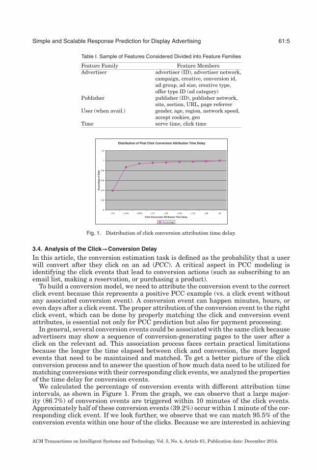
Fig. 1. Distribution of click conversion attribution time delay.
3.4. Analysis of the Click→Conversion Delay
In this article, the conversion estimation task is defined as the probability that a userwill convert after they click on an ad (PCC). A critical aspect in PCC modeling isidentifying the click events that lead to conversion actions (such as subscribing to anemail list, making a reservation, or purchasing a product).
To build a conversion model, we need to attribute the conversion event to the correctclick event because this represents a positive PCC example (vs. a click event withoutany associated conversion event). A conversion event can happen minutes, hours, oreven days after a click event. The proper attribution of the conversion event to the rightclick event, which can be done by properly matching the click and conversion eventattributes, is essential not only for PCC prediction but also for payment processing.
In general, several conversion events could be associated with the same click becauseadvertisers may show a sequence of conversion-generating pages to the user after aclick on the relevant ad. This association process faces certain practical limitationsbecause the longer the time elapsed between click and conversion, the more loggedevents that need to be maintained and matched. To get a better picture of the clickconversion process and to answer the question of how much data need to be utilized formatching conversions with their corresponding click events, we analyzed the propertiesof the time delay for conversion events.
We calculated the percentage of conversion events with different attribution timeintervals, as shown in Figure 1. From the graph, we can observe that a large major-ity (86.7%) of conversion events are triggered within 10 minutes of the click events.Approximately half of these conversion events (39.2%) occur within 1 minute of the cor-responding click event. If we look further, we observe that we can match 95.5% of theconversion events within one hour of the clicks. Because we are interested in achieving
ACM Transactions on Intelligent Systems and Technology, Vol. 5, No. 4, Article 61, Publication date: December 2014.

61:6 O. Chapelle et al.
the largest possible recall within practical boundaries, we decided to consider variousdays of delay. Within two days of the click, 98.5% of the conversions can be recovered.
These considerations are important for modeling and, in particular, for buildingproper training/test sets. The use of too short a time window would generate inaccu-rate datasets, whereas the use of too large a time window is impractical because the re-quirements for data storage and matching (click conversion) could become prohibitive.Given the just described experiments and data, we would be ignoring approximately1.5% of the conversion events and, as a consequence, incorrectly labeling a click eventas negative (no conversion) if the time frame set for post click conversion attributionis limited to two days. This was believed to be sufficient, given the practical cost oflooking further in time; thus, we utilize this limit throughout the article.
In contrast to conversions, a click can be relatively easily attributed to a particularad impression because there is a direct association between a click with the page wherethe ad is displayed. The large majority of ad clicks (97%) occur within a minute of thead impression.
4. MODELING
This section describes the various modeling techniques used to learn a response pre-dictor from clicks or conversions logs.
4.1. Logistic Regression
The model considered in this article is Maximum Entropy [Nigam et al. 1999] (a.k.a.Logistic Regression [Menard 2001]).
Given a training set (xi, yi) with xi ∈ {0, 1}d a sparse binary feature vector in a d-dimensional space, and yi ∈ {−1, 1} a binary target, the goal is to find a weight vector1
w ∈ Rd. The predicted probability of an example x belonging to class 1 is:
Pr(y = 1 | x, w) = 11 + exp(−w�x)
.
The logistic regression model is a linear model of the log odds ratio:
logPr(y = 1 | x, w)
Pr(y = −1 | x, w)= w�x. (1)
The weight vector w is found by minimizing the negative log likelihood with an L2regularization term on the weight vector:
minw
λ
2‖w‖2 +
n∑i=1
log(1 + exp(−yiw�xi)). (2)
Equation (2) is a convex, unconstrained and differentiable optimization problem.It can be solved with any gradient-based optimization technique. We use L-BFGS[Nocedal 1980], a state-of-the-art optimizer. A review of different optimization tech-niques for logistic regression can be found in Minka [2003].
4.2. Categorical Variables
All the features considered in this article are categorical. Indeed, most features areidentifiers (ID of the advertiser, of the publisher, etc.). And real valued features can bemade categorical through discretization.
The standard way of encoding categorical features is to use several binary features,known as dummy coding in statistics or the 1-of-c encoding in machine learning. If
1The intercept is one of the weights.
ACM Transactions on Intelligent Systems and Technology, Vol. 5, No. 4, Article 61, Publication date: December 2014.

Simple and Scalable Response Prediction for Display Advertising 61:7
the feature can take c values, c binary features are introduced, the ith one being theindicator function of the ith value. For instance, a feature taking the second value outof five possibles values is encoded as
(0, 1, 0, 0, 0).
If we have F features and the f -th feature can take c f values, this encoding will leadto a dimensionality of
d =F∑
f =1
c f .
4.3. Hashing Trick
The issue with the dummy coding just presented is that the dimensionality d canget very large when there are variables of high cardinality. The hashing trick, madepopular by the Vowpal Wabbit learning software and first published in Weinbergeret al. [2009], addresses this issue.
The idea is to use a hash function to reduce the number of values a feature can take.We still make use of the dummy coding described in the previous section, but insteadof a c-dimensional code, we end up with a d-dimensional one, where d is the number ofbins used with hashing. If d < c, this results in a compressed representation. In thatcase, collisions are bound to occur, but, as explained later, this is not a major concern.
When dealing with several features, there are two possible strategies:
(1) Hash each feature f into a df -dimensional space and concatenate the codes, result-ing in
∑df dimensions.
(2) Hash all features into the same space; a different hash function is used for eachfeature.
We use the latter approach because it is easier to implement.2 A summary of thehashing trick is given in Algorithm 1. The values v f can be of any type; the hashfunction only acts on their internal representation. In Algorithm 1, there is a hashingfunction hf for every feature f . This can be implemented using a single hash functionand having f as the seed or concatenating f to the value v f to be hashed.
ALGORITHM 1: Hashing TrickRequire: Values for the F features, v1, . . . , vF .Require: Family of hash function hf , number of bins d.
xi ← 0, 1 ≤ i ≤ d.for f = 1 . . . F do
i ← [hf (v f ) mod d] + 1.xi ← xi + 1
end forReturn (x1, . . . , xd).
There are some other ways of reducing the dimensionality of the model, such asdiscarding infrequent values, but they require more data processing and the use of adictionary. A very practical appeal of the hashing trick is its simplicity: It does notrequire any additional data processing or data storage, and it is straightforward toimplement.
2This is also what is implemented in Vowpal Wabbit.
ACM Transactions on Intelligent Systems and Technology, Vol. 5, No. 4, Article 61, Publication date: December 2014.

61:8 O. Chapelle et al.
4.4. Collision Analysis
We quantify in this section the log-likelihood degradation due to two values collidinginto the same bin.
Consider the scenario when the first value has been observed n1 times, all on negativeexamples, and the second value n2 times, all on positive examples, and when there isonly one feature in the system (no fallback on other features). If there were no collision,the weight for the value would be −∞ (assuming no regularization), and the weightfor the second value would be +∞. This would lead to a log likelihood of zero on all theexamples where either value is present.
When there is a collision, the negative log likelihood is:
−n1 logn1
n1 + n2− n2 log
n2
n1 + n2.
This is indeed the log likelihood achieved by the solution where all the weights are at0 except the one where there is a collision and which has a value log(n2/n1).
This log likelihood is large only when both n1 and n2 are large. This scenario can beconsidered a worst-case one because:
(1) The two values were extremely predictive: If these two values were not predictive,their collision would not harm the log likelihood (zero weight in all cases);
(2) There was no redundancy in features: If the system includes redundant features,a collision on one value could be mitigated by another value.
Regarding the last point, one could alleviate the collision issue by making use ofmultiple hash functions, in the same spirit as in the Bloom filter [Bloom 1970]. However,in practice, this does not improve the results (see Section 5.7).
This section provides only a rudimentary analysis of collisions. Given the recentinterest in hashing for categorical variables, we expect and hope that a more thoroughand theoretical analysis of the effect of collisions within a learning system will bedeveloped in the years to come.
4.5. Conjunctions
A linear model can only learn effects independently for each feature. For instance,imagine a model with two categorical features, advertiser and publisher. The modelwould learn that some advertisers and some publishers tend to have a higher CTR thanothers, but it would not learn that the CTR of a bank of america ad is particularlyhigh on finance.yahoo.com. For this, we need to introduce a new conjunction featurethat is the cartesian product of advertiser and publisher.
A conjunction between two categorical variables of cardinality c1 and c2 is just an-other categorical variable of cardinality c1 × c2. If c1 and c2 are large, the conjunctionfeature has high cardinality, and the use of the hashing trick is even more crucial inthis case.
Note that computing conjunctions between all features is equivalent to consideringa polynomial kernel of degree 2 [Scholkopf and Smola 2001] where the mapping iscomputed explicitly, as in Chang et al. [2010].
Due to the large cardinality of the representation, there will most likely be pairs ofvariable values that are unseen in the training data. And these pairs, take (adver-tiser, publisher) for instance, are biased by the current serving scheme because specificadvertisers are selected for a given publisher. The hashing trick helps reduce the di-mensionality of data but might do a poor job on these unseen pairs of values due tocollisions. This can be problematic, especially in an exploration setting where predic-tions on infrequent values are required. A possible solution is to represent the variablevalues using a low-dimensional representation, for example through the use of matrix
ACM Transactions on Intelligent Systems and Technology, Vol. 5, No. 4, Article 61, Publication date: December 2014.

Simple and Scalable Response Prediction for Display Advertising 61:9
factorization or a related approach [Menon et al. 2011]. This type of representation isnot studied in this article. A promising future work direction would be to combine alow-dimensional representation with the hashing trick: The former would capture thegeneral trend in the data, while the latter could be used to refine the model for thefrequent pairs observed in the training set.
4.6. Multitask Learning
We show in this section how multitask learning, as presented in Evgeniou and Pontil[2004], is equivalent to a single model with conjunctions, as presented in this article.
Assume that we are given T learning tasks indexed by t ∈ {1, 2, . . . , T } and a trainingset (xt
1, yt1), . . . , (xt
nt, yt
nt) for each of these tasks. The tasks are supposed to be different
but related. A task could, for instance, learn a prediction function in a given country.Evgeniou and Pontil [2004] adapted Support Vector Machines to multitask learning bydecomposing the weight vector for task t as
wt = w0 + vt,
where w0 can be interpreted as a global classifier capturing what is common among allthe tasks, and vt is a small vector modeling what is specific for that task.
The joint optimization problem is then to minimize the following cost:
T∑t=1
nt∑i=1
�((w0 + vt)�xt
i
) + λ0‖w0‖22 + λ1
T∑t=1
‖vt‖22, (3)
where � is a given loss function.Note that the relative value between λ0 and λ1 controls the strength of the connection
between the tasks. In the extreme case, if λ0 → ∞, then w0 = 0, and all tasks aredecoupled; on the other hand, when λ1 → ∞, we obtain vt = 0, and all the tasks sharethe same prediction function.
Instead of explicitly building these classifiers, an equivalent way of obtaining thesame result is to optimize a single weight vector w := [w�
0 v�1 . . . v�
T ]� and introduceconjunction features between the task and all the other features. The following vectoris thus implicitly constructed: xt
i := [xti�0� . . . xt
i�0�]�. Both approaches are indeed
equivalent when λ = λ0 = λ1 since (w0 + vt)�xti = w�xt
i and λ‖w‖22 = λ0‖w0‖2
2 +λ1
∑Tt=1 ‖vt‖2
2. The case λ0 = λ1 can be handled by putting a weight√
λ0/λ1 on theconjunction features.3
As already noted in Weinberger et al. [2009], the use of conjunction features isa powerful tool because it encompasses the multitask learning framework. Its mainadvantage is that a specific multitask solver is unnecessary: A single model is trainedwith a standard logistic regression solver.
4.7. Subsampling
Since the training data are large (around 9B impressions daily), it would be computa-tionally infeasible to consider all impressions.4 On the other hand, the training dataare very imbalanced – the CTR is lower than 1%. For these reasons, we decided tosubsample the negative class at a rate r � 1.
3One way to see that is to perform the change of variable vt ← √λ1/λ0vt.
4Infeasible on a single machine but would in fact be possible with the distributed learning system describedlater.
ACM Transactions on Intelligent Systems and Technology, Vol. 5, No. 4, Article 61, Publication date: December 2014.

61:10 O. Chapelle et al.
The model has, of course, to be corrected for this subsampling. Let us call Pr′ theprobability distribution after subsampling. Then:
Pr(y = 1 | x)Pr(y = −1 | x)
= Pr(x | y = 1) Pr(y = 1)Pr(x | y = −1) Pr(y = −1)
(4)
= Pr′(x | y = 1) Pr′(y = 1)Pr′(x | y = −1) Pr′(y = −1)/r
(5)
= rPr′(y = 1 | x)
Pr′(y = −1 | x)(6)
These equations rely on the fact that the class conditional distributions are notaffected by the subsampling: Pr(x | y) = Pr′(x | y). Combining Equations (1) and (6)results in the log odds ratio being shifted by log r. Thus, after training, the intercept ofthe model has to be corrected by adding log r to it. Logistic regression with unbalancedclasses has been well studied in the literature; more details can be found in King andZeng [2001] and Owen [2007].
Instead of shifting the intercept, another possibility would be to give an importanceweight of 1/r to the negatives samples correct for the subsampling. Preliminary exper-iments with this solution showed a lower test accuracy. A potential explanation is thatgeneralization error bounds are worse with importance weighting [Cortes et al. 2010].
4.8. Regularization and Smoothing
4.8.1. Single Feature. We draw in this section a connection between Tikhonov regular-ization as used in this article and Laplace smoothing.
Suppose that our model contains a single categorical feature. Let us consider thej-th value of that feature:
w∗ = arg minw
∑i∈Ij
log(1 + exp(−yiw)) + λ
2w2 (7)
with Ij = {i, xi = j}. When there is no regularization (λ = 0), the closed form solutionfor w∗ is:
w∗ = logk
m− kwith k = |{i ∈ Ij, yi = 1}| and m = |Ij |.
This leads to a prediction equal to k/m, which is the empirical probability P(y = 1|x =xj). We have just rederived that the logistic loss yields a Fisher consistent estimate ofthe output probability.
This empirical probability may have a large variance when m is small; thus, peopleoften use a beta prior to get a biased but lower variance estimator:
k + α
m+ 2α. (8)
This estimator is referred to as the Laplace estimator.The regularizer in Equation (7) is another way of smoothing the probability estimate
toward 0.5. These two methods are generally not equivalent, but they are related. Thefollowing proposition shows that the smoothing is similar asymptotically.
ACM Transactions on Intelligent Systems and Technology, Vol. 5, No. 4, Article 61, Publication date: December 2014.

Simple and Scalable Response Prediction for Display Advertising 61:11
Fig. 2. Smoothed probability computed from 100 success and 1,000 trials. The smoothing is achieved byregularization, as in Equation (7) or a beta prior, as in Equation (8).
PROPOSITION 4.1. When α → ∞ and w∗ is the minimizer of Equation (7) with λ = α/2,the following asymptotic equivalence holds:
11 + exp(−w∗)
− 12
∼ k + α
m+ 2α− 1
2
PROOF. At the optimum, the derivative of Equation (7) should be 0:
−kexp(−w∗)
1 + exp(−w∗)+ (m− k)
11 + exp(−w∗)
+ λw∗ = 0.
As λ → ∞, w∗ → 0 and the above equality implies that
w∗ ∼ 2k − m2λ
.
We also have1
1 + exp(−w∗)− 1
2∼ w∗
4,
andk + α
m+ 2α− 1
2∼ 2k − m
4α.
Combining these three asymptotic equivalences yields the desired result.
This proposition is illustrated in Figure 2: Regularization and smoothing with a betaprior give similar smoothed probabilities.
4.8.2. Hierarchical Feature. Consider now the case of two features having a hierarchicalrelationship, such as advertiser and campaign. Suppose that we have a lot of trainingdata for a given advertiser, but very little for a given campaign of that advertiser.Because of the regularization, the weight for that campaign will be almost zero. Thus,the predicted CTR of that campaign will mostly depend on advertiser weight. Thisis similar to the situation in the previous section except that the output probabilityis not smoothed toward 0.5 but toward the output probability given by the parentfeature.
ACM Transactions on Intelligent Systems and Technology, Vol. 5, No. 4, Article 61, Publication date: December 2014.
61:12 O. Chapelle et al.
Fig. 3. Log likelihood on a test as a function of the model size for different dimensionality reductionstrategies.
This kind of hierarchical smoothing is common in language models [Chen and Good-man 1999]. See also Gelman and Hill [2006] for a review of multilevel hierarchicalmodels and Agarwal et al. [2010] for hierarchical smoothing in display advertising.
The advantage of the logistic regression approach with regularization is that it im-plicitly performs hierarchical smoothing: Unlike the works just mentioned, we do notneed to specify the feature hierarchy.
4.9. Bayesian Logistic Regression
As we will see in Section 7, it is convenient to have a Bayesian interpretation of logisticregression [Bishop 2006, Section 4.5].
The solution of Equation (2) can be interpreted as the Maximum a Posteriori (MAP)solution of a probabilistic model with a logistic likelihood and a Gaussian prior on theweights with standard deviation 1/
√λ. There is no analytical form for the posterior
distribution Pr(w | D) ∝ ∏ni=1 Pr(yi | xi, w) Pr(w), but it can be approximated by a
Gaussian distribution using the Laplace approximation [Bishop 2006, Section 4.4].That approximation with a diagonal covariance matrix gives:
Pr(w | D) ≈ N (μ,�) with μ = arg minw
L(w) and �−1ii = ∂2L(w)
∂w2i
,
and L(w) := − log Pr(w | D) is given in Equation (2).
5. MODELING RESULTS
5.1. Experimental Setup
The experimental results presented in this section have been obtained in various con-ditions (training set, features, evaluation). Most of them were based on the RMX datadescribed in Section 3, but some of the experiments—those in Figures 3, 4, and 5 andSection 5.6—have been run on logs from Criteo, a large display advertising company.
Even though the details of the experimental setups varied, they were all similar,with the following characteristics. The training and test sets are split chronologically,both with periods ranging from several days to several weeks. After subsampling thenegative samples as explained in Section 4.7, the number of training samples is ofthe order of one billion. The number of base features is about 30, from which several
ACM Transactions on Intelligent Systems and Technology, Vol. 5, No. 4, Article 61, Publication date: December 2014.

Simple and Scalable Response Prediction for Display Advertising 61:13
hundred conjunctions are constructed. The number of bits used for hashing was 24,resulting in a model with 16M parameters.
Depending on the experiment, the test metrics are either the negative log likelihood(NLL), root mean squared error (RMSE), area under the precision/recall curve (auPRC),or area under the ROC curve (auROC). When a metric is said to be normalized, this isthe value of the metric relative to the best constant baseline.
5.2. Hashing Trick
The first component of our system that we want to evaluate is the use of the hashingtrick. Recall that because we use features that can take a large number of values (espe-cially the conjunction features), running the logistic regression without dimensionalityreduction is infeasible.
An alternative to the hashing trick is to keep only the most important values. Comingback to the example of Section 4.2, if a feature can take five values, but only two ofthem are deemed important, we would encode that feature with two bits, both of thembeing zero when the feature value is not important.
Two simple heuristics for finding important values are:
—Count: Select the most frequent values.—Mutual information: Select the values that are most helpful in determining the
target.
A drawback of this approach is that the model needs to be stored as a dictionaryinstead of an array. The dictionary maps each important value to its weight. Thedictionary is needed to avoid collisions and to keep track of the most important values.Its size is implementation-dependent, but a lower bound can be 12 bytes per entry: 4for the key, 4 for the value, and 4 for the pointer in a linked list. Empirically, in C#, thesize is about 20–25 bytes per entry.
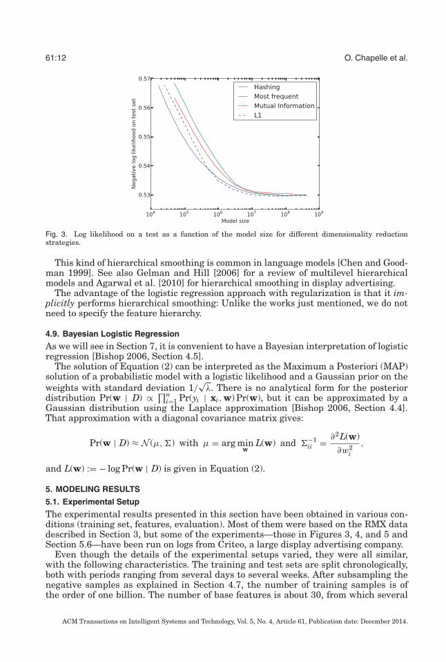
Figure 3 shows the log likelihood as a function of the model size: 4d for hashing and12d for dictionary based models, where d is the number of weights in the model. Itturns out that for the same model size, the hashing based model is slightly superior.Two other advantages are convenience (there is no need to find the most importantvalues and keep them in a dictionary) and real-time efficiency (hashing is faster than adictionary look-up).
For the sake of the comparison, Figure 3 also includes a method whereby the mostimportant values are selected through the use of a sparsity-inducing norm. This isachieved by adding an L1 norm on w in Equation (2) and minimizing the objectivefunction using a proximal method [Bach et al. 2011, chapter 3]. Each point on the curvecorresponds to a regularization parameter in the set {1, 3, 10, 30, 300, 1000, 3000}: thelarger the parameter, the sparser the model. The L2 regularization parameter is keptat the same value as for the other methods. Even though the resulting model needsto be stored in a dictionary, this method achieves a good tradeoff in terms of accuracyversus model size. Note, however, that this technique is not easily scalable: Duringtraining, it requires one weight for each value observed in the training set. This wasfeasible in Figure 3 because we considered a rather small training set with only 33Mdifferent values. But in a production setting, the number of values can easily exceed abillion.
5.3. Effect of Subsampling
The easiest way to deal with a very large training set is to subsample it. Sometimessimilar test errors can be achieved with smaller training sets, and there is no need forlarge-scale learning in these cases.
ACM Transactions on Intelligent Systems and Technology, Vol. 5, No. 4, Article 61, Publication date: December 2014.

61:14 O. Chapelle et al.
Fig. 4. Change in log likelihood by subsampling the negatives. The baseline is a model with all negativesincluded.
Table II. Test Performance Drop as a Functionof the Overall Subsampling Rate
1% 10%auROC −2.0% −0.5%auPRC −7.2% −2.1%NLL −3.2% −2.3%
Two different levels of subsampling be done: Subsampling the negatives, as dis-cussed in Section 4.7, or subsampling the entire dataset. Both speed up the trainingconsiderably, but can result in some performance drop, as shown later. The choice ofthe subsampling rates is thus an application-dependent tradeoff to be made betweencomputational complexity and accuracy.
5.3.1. Subsampling the Negatives. In this experiment, we keep all the positives and sub-sample the negatives. Figure 4 shows how much the model is degraded as a functionof the subsampling rate.
We found empirically that a subsample rate of 1% was a good tradeoff betweenmodel training time and predictive accuracy. Unless otherwise noted, the negativesare subsampled at 1% in the rest of this paper.
5.3.2. Overall Subsampling. The entire dataset has been subsampled in this experimentat 1% and 10%. The results in Table II show that there is a drop in accuracy aftersubsampling.
In summary, even if it is fine to subsample the data to some extent—the negativesin particular—the more data, the better, and this motivates the use of the distributedlearning system presented in Section 8.
5.4. Comparison with a Feedback Model
An alternative class of models used for response prediction is the feedback modelsdescribed in Hillard et al. [2010, Section 4.1]. In that approach, response rate is notencoded in the weights but in the feature values via the use of feedback features. Thisapproach relies on the observation that the average historical response rate of an ad isa good indicator of its future response rate.
Feedback features are derived by aggregating the historical data along various di-mensions (such as ads, publishers, or users) at varying levels of granularity. The cor-responding response rate (CTR or CVR) and its support (i.e., number of impressionsor clicks) are the feature values used in modeling. When the support is under some
ACM Transactions on Intelligent Systems and Technology, Vol. 5, No. 4, Article 61, Publication date: December 2014.

Simple and Scalable Response Prediction for Display Advertising 61:15
Table III. Comparison with aClick Feedback Model
auROC auPRC+0.9% +1.3%
threshold, the historical response rate is typically considered to be undefined becausethe estimate would be unreliable.
The response rate of an ad might change depending on the publisher page it is shownon or the users who see it. To capture the variation of response rate across differentdimensions, multiple attributes along different dimensions could be used to gener-ate composite feedback features (similar to conjunction features), such as publisher-advertiser and user-publisher-creative composites.
Feedback features are quantized using a simple k-means clustering algorithm [Mac-Queen 1967] (with a special cluster ID indicating the undefined values) before they arefed to the logistic regression algorithm. The size of the final models is therefore typi-cally small. However, additional memory is needed to store the feature ID to feedbackfeature value mappings. Note that feedback features are often refreshed regularly byupdating the statistics with the latest historical information available.
One potential weakness of a feedback feature is that it may give an incorrect signalbecause of confounding variables. Thus, it is preferable, as advocated in this article,to directly model the response as a function of all variables and not to perform anyaggregation.
However, from a practical standpoint, a model based on feedback features may bepreferred in cases where the cost of updating the model is substantially higher thanthe cost of updating the feedback features.
We used a relatively small number of features to do the comparison between ourproposed model based on categorical features and a model based on feedback features.Results in Table III show that both models are similar, with a slight advantage forour proposed model. The difference would likely be larger as the number of featuresincreases: The model based on categorical variables would better model the effect ofconfounding variables.
5.5. Comparison with a Hierarchical Model
Next, we compare our approach to the state-of-the-art Log-linear Model for MultipleHierarchies (LMMH) method [Agarwal et al. 2010] that has been developed in the samecontext: CTR estimation for display advertising with hierarchical features. The LMMHapproach exploits the hierarchical nature of the advertiser and publisher attributes byexplicitly encoding these relations. It splits the modeling task into two stages: First,a feature-based model is trained using covariates, without hierarchical features. Inthe second stage, the publisher (e.g., publisher type→publisher ID) and advertiserhierarchies (e.g., advertiser ID→campaign ID→ ad ID) are used to learn the correctionfactors on top of the baseline model. Expected number of clicks, E, for each publisherand advertiser hierarchy is calculated by summing up the baseline probabilities overall the samples in which that publisher and advertiser hierarchy is present. Correctionfactors of the full hierarchies are modeled as log-linear functions of pairs of advertiserand publisher nodes (e.g., {publisher type, advertiser ID}):
λhi =∏
ai∈hi,ad
∏pj∈hi,pub
φai ,pj (9)
where λhi is the multiplicative correction factor for the hierarchy pair hi, hi,ad and hi,pubare advertiser and publisher hierarchies for that pair, and φai ,pj is the state parameter
ACM Transactions on Intelligent Systems and Technology, Vol. 5, No. 4, Article 61, Publication date: December 2014.
61:16 O. Chapelle et al.
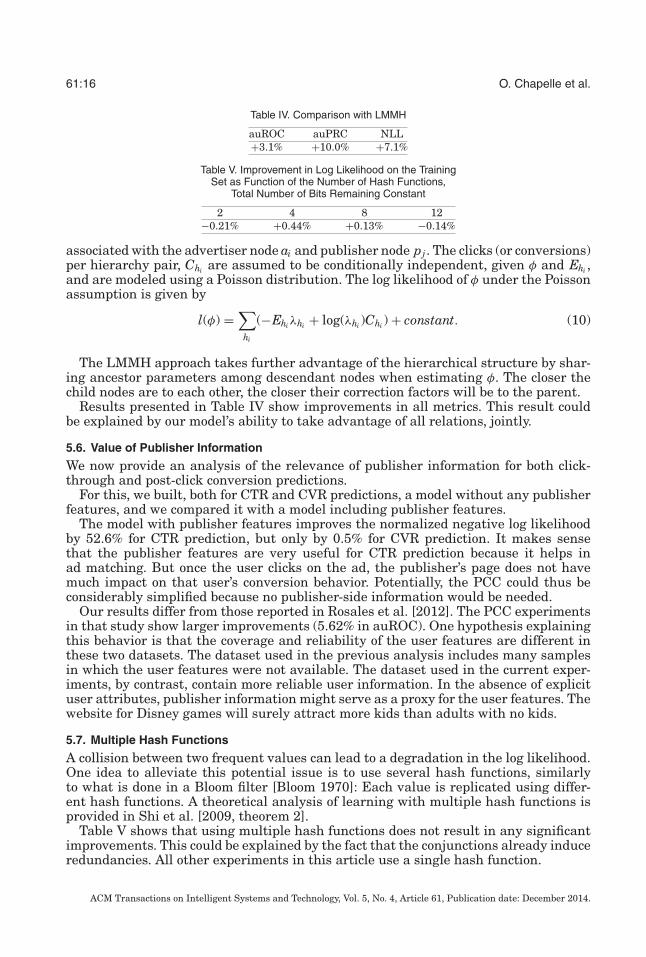
Table IV. Comparison with LMMH
auROC auPRC NLL+3.1% +10.0% +7.1%
Table V. Improvement in Log Likelihood on the TrainingSet as Function of the Number of Hash Functions,
Total Number of Bits Remaining Constant
2 4 8 12−0.21% +0.44% +0.13% −0.14%
associated with the advertiser node ai and publisher node pj . The clicks (or conversions)per hierarchy pair, Chi are assumed to be conditionally independent, given φ and Ehi ,and are modeled using a Poisson distribution. The log likelihood of φ under the Poissonassumption is given by
l(φ) =∑
hi
(−Ehi λhi + log(λhi )Chi ) + constant. (10)
The LMMH approach takes further advantage of the hierarchical structure by shar-ing ancestor parameters among descendant nodes when estimating φ. The closer thechild nodes are to each other, the closer their correction factors will be to the parent.
Results presented in Table IV show improvements in all metrics. This result couldbe explained by our model’s ability to take advantage of all relations, jointly.
5.6. Value of Publisher Information
We now provide an analysis of the relevance of publisher information for both click-through and post-click conversion predictions.
For this, we built, both for CTR and CVR predictions, a model without any publisherfeatures, and we compared it with a model including publisher features.
The model with publisher features improves the normalized negative log likelihoodby 52.6% for CTR prediction, but only by 0.5% for CVR prediction. It makes sensethat the publisher features are very useful for CTR prediction because it helps inad matching. But once the user clicks on the ad, the publisher’s page does not havemuch impact on that user’s conversion behavior. Potentially, the PCC could thus beconsiderably simplified because no publisher-side information would be needed.
Our results differ from those reported in Rosales et al. [2012]. The PCC experimentsin that study show larger improvements (5.62% in auROC). One hypothesis explainingthis behavior is that the coverage and reliability of the user features are different inthese two datasets. The dataset used in the previous analysis includes many samplesin which the user features were not available. The dataset used in the current exper-iments, by contrast, contain more reliable user information. In the absence of explicituser attributes, publisher information might serve as a proxy for the user features. Thewebsite for Disney games will surely attract more kids than adults with no kids.
5.7. Multiple Hash Functions
A collision between two frequent values can lead to a degradation in the log likelihood.One idea to alleviate this potential issue is to use several hash functions, similarlyto what is done in a Bloom filter [Bloom 1970]: Each value is replicated using differ-ent hash functions. A theoretical analysis of learning with multiple hash functions isprovided in Shi et al. [2009, theorem 2].
Table V shows that using multiple hash functions does not result in any significantimprovements. This could be explained by the fact that the conjunctions already induceredundancies. All other experiments in this article use a single hash function.
ACM Transactions on Intelligent Systems and Technology, Vol. 5, No. 4, Article 61, Publication date: December 2014.

Simple and Scalable Response Prediction for Display Advertising 61:17
6. FEATURE SELECTION
We tackle in this section the problem of feature selection for categorical variables.Let us first distinguish two different levels of selection in the context of categorical
variables:
—Feature selection. The goal is to select some of the features (such as age, gender, oradvertiser) to be included in the learning system. This is the purpose of this section.
—Value selection. The goal is to reduce the number of parameters by discarding some ofthe least important values observed in the training set. Section 5.2 compares variousschemes for this purpose.
L1 regularization is an effective way of reducing the number of parameters in thesystem and is thus a value selection method. But it does not necessarily suppress all thevalues of a given feature and cannot therefore be used for feature selection. For this, apossible regularization is the so-called �1/�2 regularization or group lasso [Meier et al.2008]. However, group lasso would be computationally expensive at the scale of dataat which we operate. We present in this section a cheaper alternative.
As for mutual information and other filter methods for feature selection [Guyon andElisseeff 2003], we are looking for a criterion that measures the utility of a feature in abinary classification task. However, the goal is to do so conditioned on already existingfeatures; that is, we want to estimate the additional utility of a feature when added toan already existing classifier [Koepke and Bilenko 2012].
6.1. Conditional Mutual Information
We assume that we already have an existing logistic regression model with a base setof features. Let si be the score predicted by this model.
The negative log likelihood of the current model is:
n∑i=1
log(1 + exp(−yisi)). (11)
Let us approximate the log-likelihood improvement we would see if we were to addthat feature to the training set.
A first approximation is to say the weights already learned are fixed and that onlythe weights associated with the new features are learned. For the sake of simplicity,let’s say the new feature takes d values and that these values are X = {1, . . . , d}. Wethus need to learn d weights w1, . . . , wd, each of them corresponding to a value of thefeature. The updated prediction with the new feature on the i-th example is then:si + wxi .
They are found by minimizing the new log likelihood:
n∑i=1
log(1 + exp(−yi(si + wxi ))),
which can be decomposed as:
d∑k=1
∑i∈Ik
log(1 + exp(−yi(si + wk))), with Ik = {i, xi = k}. (12)
ACM Transactions on Intelligent Systems and Technology, Vol. 5, No. 4, Article 61, Publication date: December 2014.

61:18 O. Chapelle et al.
This is an easy optimization problem since all wk are independent of each others:
wk = arg minw
∑i∈Ik
log(1 + exp(−yi(si + w)))
︸ ︷︷ ︸Lk(w)
.
There is, however, no closed form solution for wk. A further approximation is to setwk to the value after one Newton step starting from 0:
wk ≈ − L′k(0)
L′′k(0)
. (13)
The first and second derivatives of Lk are:
L′k(0) =
∑i∈Ik
pi − yi + 12
L′′k(0) =
∑i∈Ik
pi(1 − pi) with pi = 11 + exp(−si)
.
Once the wk are computed, the log-likelihood improvement can be measured as thedifference of Equations (12) and (11) or using the second-order approximation of thelog likelihood:
d∑k=1
wkL′k(0) + 1
2w2
k L′′k(0).
Special case. When s is constant and equal to the log odds class prior, there is a closedform solution for wk. It is the value such that
11 + exp(−s + wk)
= 1|Ik|
∑i∈Ik
yi + 12
= Pr(y = 1 | x = k).
With that value, the difference in the log likelihoods in Equations (12) and (11) is:n∑
i=1
logPr(yi | xi)
Pr(yi), (14)
which is exactly the mutual information between the variables x and y. The proposedmethod can thus be seen as an extension of mutual information to the case where somepredictions are already available.
6.2. Reference Distribution
As always in machine learning, there is an overfitting danger: It is particularly truefor features with a lot of values. Such features can improve the likelihood on thetraining set, but not necessarily on the test set. This problem has also been noted withstandard mutual information [Rosales and Chapelle 2011]. To prevent this issue, aregularization term, λw2
k, can be added to Lk. And as in Rosales and Chapelle [2011],instead of computing the log-likelihood improvement on the training set, it can be doneon a separate reference set.
The issue of computing the mutual information on the training set can be illustratedas follows: Consider a feature taking unique values (it can, for instance, be an eventidentifier), then the mutual information between that feature and the target will bemaximum since the values of that feature can fully identify the data point and thereforeits label. Formally, Equation (14) turns out to be in this case:
n∑i=1
log1
P(yi)= H(Y ),
ACM Transactions on Intelligent Systems and Technology, Vol. 5, No. 4, Article 61, Publication date: December 2014.
Simple and Scalable Response Prediction for Display Advertising 61:19
since Pr(yi | xi) = 1 if all xi are unique. And, of course, the mutual information cannever be larger than the entropy. This example shows that the mutual informationis not a good indicator of the predictiveness of a feature because it is biased towardfeatures with high cardinality. Computing the mutual information on a validation setaddresses this issue.
6.3. Results
We utilized the method just described for determining feature relevance for click pre-diction. Our main motivation was decreasing model complexity because the availablenumber of possible features is too large to be used in their entirety during predic-tion/modeling. Practical considerations, such as memory, latency, and training timeconstraints, make feature selection a clear requirement in this task.
The evaluation is divided into two parts: We first verify that computing the mu-tual information using a reference distribution gives more sensible results than thestandard mutual information; then, we evaluate the use of the conditional mutualinformation in a forward feature selection algorithm.
6.3.1. Use of a Reference Distribution. For these experiments, we considered one day ofdata for the training distribution and one day for the reference distribution.
Our goal is to identify predictive features in the most automated manner possible (re-ducing time spent by people on this task). Thus, practically all the raw (unprocessed)data attributes available were included in the analysis. These features are a super-set of those in Table I and include identifiers for the actual (serve/click/conversion)event, advertiser, publisher, campaign, cookies, timestamps, advertiser/publisher spe-cific features, related URLs, demographics, user-specific features (identifiers, assignedsegments), and the like. We consider conjunctions of any of these features, giving riseto about 5,000 possible compound features in practice. Each feature in turn can takefrom two to millions of possible values.
We remark that wrapper methods are rarely appropriate in this setting because theyrequire training using a large set of variables; this is usually impractical except forsome simple models. It is in this setting that filter methods, such as the MI methodsdescribed here, can be more advantageous.
We applied the Standard MI (SMI) ranking algorithm for feature selection. Theresults, summarized in Table VI (top) reflect our main concern. The spurious features,or features that are informative about the data point per se, rank substantially high.The calculated MI score is correct in that it reflects the information content of thesefeatures; however, these features are too specific to the training data distribution.
The proposed extension of the MI score utilizing a reference distribution (RMI) pro-vides a more appropriate ranking, as shown in Tables VI (mid-bottom) because theinformation content is calculated with respect to (expectations on) the reference dis-tribution; thus, feature values that are not seen in the new distribution are basicallyconsidered less important and their impact on the information score is reduced.
More specifically, attributes such as event_guid that identifies the data point havemaximal information content according to the training distribution (SMI), but nearzero information content when calculated with a reference distribution (RMI). A similareffect was observed for other features that have low relevance for prediction, such asquery_string and receive_time which, unless parsed, are too specific; xcookie anduser_identifier, which clearly do not generalize across users (but could be quiteinformative about a small fraction of the test data); and user_segments, which indexesuser categories. The results for other features are more subtle but follow the sameunderlying principle in which a reference distribution is utilized to avoid spuriousdependencies often found when utilizing empirical distributions.
ACM Transactions on Intelligent Systems and Technology, Vol. 5, No. 4, Article 61, Publication date: December 2014.

61:20 O. Chapelle et al.
Table VI. Top Features for Click Prediction Alongwith Their Mutual Information
Single Feature SMI (bits)event_guid 0.59742query_string 0.59479xcookie 0.49983user_identifier 0.49842user_segments 0.43032
Single feature RMI (bits)section_id 0.20747creative_id 0.20645site 0.19835campaign_id 0.19142rm_ad_grp_id 0.19094
Conjunction feature RMI (bits)section_id x advertiser_id 0.24691section_id x creative_id 0.24317section_id x IO_id 0.24307creative_id x publisher_id 0.24250creative_id x site 0.24246site x advertiser_id 0.24234section_id x pixeloffers 0.24172site x IO_id 0.23953publisher_id x advertiser_id 0.23903
First table: standard mutual information; second and thirdtable: modified mutual information (RMI). Bottom sectioncontains the top conjunction features.
6.3.2. Learning Performance Results. Here, we explore the question of automatically find-ing new conjunction features and whether these features actually offer any perfor-mance gains. For this, we use the conditional mutual information within a forwardfeature selection algorithm:
(1) Start with a set of base features and no conjunction features;(2) Train a model with all the selected features;(3) Compute the conditional mutual information for all conjunctions not yet selected;(4) Select the best conjunction;(5) Go back to (2).
The results of this procedure are shown in Figure 5. It can be seen that selecting 50features in this way has a twofold advantage over including the 351 possible conjunc-tions: It results in a model with fewer features (faster to train and evaluate), and itgeneralizes better.
7. NONSTATIONARITY
Display advertising is a nonstationary process because the set of active advertis-ers, campaigns, publishers, and users is constantly changing. We first quantify thesechanges in Sections 7.1 and 7.2, then show in Section 7.3 how to efficiently update themodel to take into account the nonstationarity of the data. We discuss Thompson sam-pling in Section 7.4 and later as a way to address the explore/exploit tradeoff necessaryin this kind of dynamic environment.
7.1. Ad Creation Rates
Response prediction models are trained using historical logs. When completely newads are added to the system, models built on past data may not perform as well,
ACM Transactions on Intelligent Systems and Technology, Vol. 5, No. 4, Article 61, Publication date: December 2014.
Simple and Scalable Response Prediction for Display Advertising 61:21
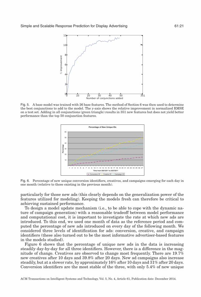
Fig. 5. A base model was trained with 26 base features. The method of Section 6 was then used to determinethe best conjunctions to add to the model. The y-axis shows the relative improvement in normalized RMSEon a test set. Adding in all conjunctions (green triangle) results in 351 new features but does not yield betterperformance than the top 50 conjunction features.
Fig. 6. Percentage of new unique conversion identifiers, creatives, and campaigns emerging for each day inone month (relative to those existing in the previous month).
particularly for those new ads (this clearly depends on the generalization power of thefeatures utilized for modeling). Keeping the models fresh can therefore be critical toachieving sustained performance.
To design a model update mechanism (i.e., to be able to cope with the dynamic na-ture of campaign generation) with a reasonable tradeoff between model performanceand computational cost, it is important to investigate the rate at which new ads areintroduced. To this end, we used one month of data as the reference period and com-puted the percentage of new ads introduced on every day of the following month. Weconsidered three levels of identification for ads: conversion, creative, and campaignidentifiers (these also turned out to be the most informative advertiser-based featuresin the models studied).
Figure 6 shows that the percentage of unique new ads in the data is increasingsteadily day-by-day for all three identifiers. However, there is a difference in the mag-nitude of change. Creatives are observed to change most frequently. There are 19.7%new creatives after 10 days and 39.8% after 20 days. New ad campaigns also increasesteadily, but at a slower rate, by approximately 16% after 10 days and 31% after 20 days.Conversion identifiers are the most stable of the three, with only 5.4% of new unique
ACM Transactions on Intelligent Systems and Technology, Vol. 5, No. 4, Article 61, Publication date: December 2014.
61:22 O. Chapelle et al.
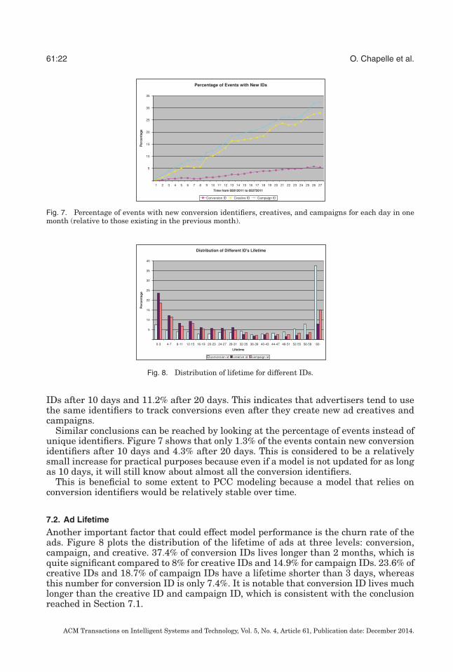
Fig. 7. Percentage of events with new conversion identifiers, creatives, and campaigns for each day in onemonth (relative to those existing in the previous month).
Fig. 8. Distribution of lifetime for different IDs.
IDs after 10 days and 11.2% after 20 days. This indicates that advertisers tend to usethe same identifiers to track conversions even after they create new ad creatives andcampaigns.
Similar conclusions can be reached by looking at the percentage of events instead ofunique identifiers. Figure 7 shows that only 1.3% of the events contain new conversionidentifiers after 10 days and 4.3% after 20 days. This is considered to be a relativelysmall increase for practical purposes because even if a model is not updated for as longas 10 days, it will still know about almost all the conversion identifiers.
This is beneficial to some extent to PCC modeling because a model that relies onconversion identifiers would be relatively stable over time.
7.2. Ad Lifetime
Another important factor that could effect model performance is the churn rate of theads. Figure 8 plots the distribution of the lifetime of ads at three levels: conversion,campaign, and creative. 37.4% of conversion IDs lives longer than 2 months, which isquite significant compared to 8% for creative IDs and 14.9% for campaign IDs. 23.6% ofcreative IDs and 18.7% of campaign IDs have a lifetime shorter than 3 days, whereasthis number for conversion ID is only 7.4%. It is notable that conversion ID lives muchlonger than the creative ID and campaign ID, which is consistent with the conclusionreached in Section 7.1.
ACM Transactions on Intelligent Systems and Technology, Vol. 5, No. 4, Article 61, Publication date: December 2014.

Simple and Scalable Response Prediction for Display Advertising 61:23
Fig. 9. The performance (auROC) of the model degrades with time.
7.3. Model Update
The results in Sections 7.1 and 7.2 indicate that there is a nontrivial percentage ofnew ads entering the system every day. In this section, we first illustrate the impactthat this has on a static post-click conversion model, and later provide an algorithm toupdate our models efficiently.
In this analysis, data collected from a given month are used for training, and data ofthe following month are used as test data.
To evaluate the impact of the new ads on the model performance, we divided the testdata into daily slices. In Figure 9, we present the performance of the static model. Thex-axis represents each day in the test data, and the y-axis indicates the auROC. Wecan see from Figure 9 that the performance of the model degrades with time.
It is clear that the degradation in performance is closely related to the influx rateof new ads in the test data, as elucidated in previous analyses (Sections 7.1–7.2). Forthis reason, we cannot use a static model; we need to continuously refresh it with newdata, as explained below.
The Bayesian interpretation of logistic regression described in Section 4.9 can beleveraged for model updates. Remember that the posterior distribution on the weightsis approximated by a Gaussian distribution with diagonal covariance matrix. As in theLaplace approximation, the mean of this distribution is the mode of the posterior, andthe inverse variance of each weight is given by the curvature. The use of this convenientapproximation of the posterior is twofold. It first serves as a prior on the weights toupdate the model when a new batch of training data becomes available, as describedin Algorithm 2. And it is also the distribution used in the exploration/exploitationheuristic described in the next section.
To illustrate the benefits of model updates, we performed the following experiment.We considered 3 weeks of training data and 1 week of test data. A base model is trainedon the training data. The performance with model updates is measured as follows:
(1) Split the test set in n = 24 × 7/k batches of k hours;(2) For i = 1, . . . , n:
—Test the current model on the i-th batch—Use the i-th batch of data to update the model as explained in Algorithm 2.
The baseline is the static base model applied to the entire test data. As shown in TableVII, the more frequently the model is updated, the better its accuracy.
ACM Transactions on Intelligent Systems and Technology, Vol. 5, No. 4, Article 61, Publication date: December 2014.

61:24 O. Chapelle et al.
Table VII. Influence of the UpdateFrequency (Area under the PR Curve)
1 day 6 hours 2 hours+3.7% +5.1% +5.8%
ALGORITHM 2: Regularized Logistic Regression with Batch UpdatesRequire: Regularization parameter λ > 0.
mi = 0, qi = λ. {Each weight wi has an independent prior N (mi, q−1i )}
for t = 1, . . . , T doGet a new batch of training data (x j, yj), j = 1, . . . , n.
Find w as the minimizer of:12
d∑i=1
qi(wi − mi)2 +n∑
j=1
log(1 + exp(−yjw�x j)).
mi = wi
qi = qi +n∑
j=1
x2i j pj(1 − pj), pj = (1 + exp(−w�x j))−1 {Laplace approximation}
end for
7.4. Exploration/Exploitation Tradeoff
To learn the CTR of a new ad, it needs to be displayed first, leading to a potential lossof short-term revenue. This is the classical exploration/exploitation dilemma: Eitherexploit the best ad observed so far, or take a risk and explore new ones resulting in eithera short-term loss or a long-term profit depending on whether that ad is worse or better.
Various algorithms have been proposed to solve exploration/exploitation or banditproblems. One of the most popular one is the Upper Confidence Bound (UCB) [Laiand Robbins 1985; Auer et al. 2002] for which theoretical guarantees on the regretcan be proved. Another representative is the Bayes-optimal approach of Gittins [1989]that directly maximizes expected cumulative payoffs with respect to a given priordistribution. A less known family of algorithms is so-called probability matching. Theidea of this heuristic is old and dates back to Thompson [1933]; thus, this scheme is alsoreferred to as Thompson sampling in the literature. The idea of Thompson samplingis to randomly draw each arm according to its probability of being optimal. In contrastto a full Bayesian method like the Gittins index, one can often implement Thompsonsampling efficiently.
7.5. Thompson Sampling
In this section, we present a general description of Thompson sampling and providesome experimental results in the next one. More details can be found in Chapelle andLi [2011].
The contextual bandit setting is as follows: At each round, we have a context x(optional) and a set of actions A. After choosing an action a ∈ A, we observe a rewardr. The goal is to find a policy that selects actions such that the cumulative reward is aslarge as possible.
Thompson sampling is best understood in a Bayesian setting as follows: The set ofpast observations D is made of triplets (xi, ai, ri) and are modeled using a parametriclikelihood function P(r|a, x, θ ) depending on some parameters θ . Given some priordistribution P(θ ) on these parameters, the posterior distribution of these parametersis given by the Bayes rule, P(θ |D) ∝ ∏
P(ri|ai, xi, θ )P(θ ).In the realizable case, the reward is a stochastic function of the action, context, and
the unknown true parameter θ∗. Ideally, we would like to choose the action maximizingthe expected reward, maxa E(r|a, x, θ∗).
ACM Transactions on Intelligent Systems and Technology, Vol. 5, No. 4, Article 61, Publication date: December 2014.

Simple and Scalable Response Prediction for Display Advertising 61:25
Of course, θ∗ is unknown. If we are just interested in maximizing the immediatereward (exploitation), then one should choose the action that maximizes E(r|a, x) =∫
E(r|a, x, θ )P(θ |D)dθ .But in an exploration/exploitation setting, the probability matching heuristic consists
in randomly selecting an action a according to its probability of being optimal. That is,action a is chosen with probability∫
I
[E(r|a, x, θ ) = max
a′E(r|a′, x, θ )
]P(θ |D)dθ,
where I is the indicator function. Note that the integral does not have to be computedexplicitly: It suffices to draw a random parameter θ at each round, as explained inAlgorithm 3. The implementation is thus efficient and straightforward in our appli-cation: Since the posterior is approximated by a Gaussian distribution with diagonalcovariance matrix (see Section 4.9), each weight is drawn independently from a Gaus-sian distribution.
ALGORITHM 3: Thompson SamplingD = ∅for t = 1, . . . , T do
Receive context xtDraw θ t according to P(θ |D)Select at = arg maxa Er(r|xt, a, θ t)Observe reward rtD = D ∪ (xt, at, rt)
end for
In addition to being a good heuristic for explore/exploit, the advantage of Thompsonsampling is that the randomized predictions it generates are compatible with a gen-eralized second price auction, as typically used in ad exchanges. In other words, theauction is still incentive-compatible even though the predictions are randomized [Meeket al. 2005, Example 2]. It would be unclear which generalized second price to chargewith other explore/exploit strategies.
7.6. Evaluation of Thomson Sampling
Evaluating an explore/exploit policy is difficult because we typically do not know thereward of an action that was not chosen. A possible solution is to use a replayer,in which previous, randomized exploration data can be used to produce an unbiasedoffline estimator of the new policy [Li et al. 2011]. Unfortunately, this approach cannotbe used in our case because it reduces the effective data size substantially when thenumber of arms K is large, yielding too high variance in the evaluation results.
For the sake of simplicity, therefore, we considered in this section a simulated envi-ronment. More precisely, the context and the ads are real, but the clicks are simulatedusing a weight vector w∗. This weight vector could have been chosen arbitrarily, but itwas in fact a perturbed version of some weight vector learned from real clicks. The in-put feature vectors x are thus as in the real-world setting, but the clicks are artificiallygenerated with probability P(y = 1|x) = (1 + exp(−w∗�x))−1.
About 13,000 contexts, representing a small random subset of the total traffic, arepresented every hour to the policy, which then has to choose an ad among a set of eligibleads. The number of eligible ads for each context depends on numerous constraints setby the advertiser and the publisher. It varies between 5,910 and 1, with a mean of1,364 and a median of 514 (over a set of 66,373 ads). Note that in this experiment the
ACM Transactions on Intelligent Systems and Technology, Vol. 5, No. 4, Article 61, Publication date: December 2014.

61:26 O. Chapelle et al.
Table VIII. CTR Regrets for Different Explore/Exploit Strategies
Method TS LinUCB ε-greedyParameter 0.25 0.5 1 0.5 1 2 0.005 0.01 0.02 Exploit RandomRegret (%) 4.45 3.72 3.81 4.99 4.22 4.14 5.05 4.98 5.22 5.00 31.95
number of eligible ads is smaller than what we would observe in live traffic because werestricted the set of advertisers.
The model is updated every hour, as described in Algorithm 2. A feature vector isconstructed for every (context, ad) pair and the policy decides which ad to show. A clickfor that ad is then generated with probability (1+exp(−w∗�x))−1. This labeled trainingsample is then used at the end of the hour to update the model. The total number ofclicks received during this one-hour period is the reward. To eliminate unnecessaryvariance in the estimation, we instead computed the expectation of that number sincethe click probabilities are known.
Several explore/exploit strategies are compared; they only differ in the way the adsare selected—all the rest, including the model updates, is identical, as described inAlgorithm 2. These strategies are:
—Thompson sampling. This is Algorithm 3, in which each weight is drawn in-dependently according to its Gaussian posterior approximation N (mi, q−1
i ) (seeAlgorithm 2). We also consider a variant in which the standard deviations q−1/2
i arefirst multiplied by a factor α ∈ {0.25, 0.5}. This favors exploitation over exploration.
—LinUCB. This is an extension of the UCB algorithm to the parametric case [Li et al.2010]. It selects the ad based on mean and standard deviation. It also has a factor αto control the exploration/exploitation tradeoff. More precisely, LinUCB selects the
ad for which∑d
i=1 mixi + α
√∑di=1 q−1
i x2i is maximum.
—Exploit-only. Select the ad with the highest mean.—Random. Select the ad uniformly at random.—ε-greedy. Mix between exploitation and random: With ε probability, select a random
ad; otherwise, select the one with the highest mean.
Results. A preliminary result is about the quality of the variance prediction. Thediagonal Gaussian approximation of the posterior does not seem to harm the variancepredictions. In particular, they are very well calibrated: When constructing a 95%confidence interval for CTR, the true CTR is in this interval 95.1% of the time.
The regrets of the different explore/exploit strategies can be found in Table VIII.Thompson sampling achieves the best regret, and, interestingly, the modified versionwith α = 0.5 gives slightly better results than the standard version (α = 1).
Exploit-only does pretty well, at least compared to random selection. This seems atfirst a bit surprising given that the system has no prior knowledge about the CTRs. Apossible explanation is that the change in context induces some exploration, as notedin Sarkar [1991]. Also, the fact that exploit-only is so much better than random mightexplain why ε-greedy does not beat it: Whenever this strategy chooses a random action,it suffers a large regret on average, which is not compensated by its exploration benefit.
Finally, Figure 10 shows the regret of three algorithms across time. As expected, theregret has a decreasing trend over time.
8. LARGE-SCALE LEARNING
Because of the large amount of data, we use the distributed Hadoop-based learningsystem [Agarwal et al. 2011]. This section presents a summary of this system withsome experimental results.
ACM Transactions on Intelligent Systems and Technology, Vol. 5, No. 4, Article 61, Publication date: December 2014.
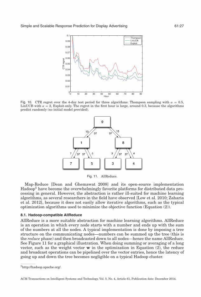
Simple and Scalable Response Prediction for Display Advertising 61:27
Fig. 10. CTR regret over the 4-day test period for three algorithms: Thompson sampling with α = 0.5,LinUCB with α = 2, Exploit-only. The regret in the first hour is large, around 0.3, because the algorithmspredict randomly (no initial model provided).
Fig. 11. AllReduce.
Map-Reduce [Dean and Ghemawat 2008] and its open-source implementationHadoop5 have become the overwhelmingly favorite platforms for distributed data pro-cessing in general. However, the abstraction is rather ill-suited for machine learningalgorithms, as several researchers in the field have observed [Low et al. 2010; Zahariaet al. 2012], because it does not easily allow iterative algorithms, such as the typicaloptimization algorithms used to minimize the objective function (Equation (2)).
8.1. Hadoop-compatible AllReduce
AllReduce is a more suitable abstraction for machine learning algorithms. AllReduceis an operation in which every node starts with a number and ends up with the sumof the numbers at all the nodes. A typical implementation is done by imposing a treestructure on the communicating nodes—numbers can be summed up the tree (this isthe reduce phase) and then broadcasted down to all nodes—hence the name AllReduce.See Figure 11 for a graphical illustration. When doing summing or averaging of a longvector, such as the weight vector w in the optimization in Equation (2), the reduceand broadcast operations can be pipelined over the vector entries, hence the latency ofgoing up and down the tree becomes negligible on a typical Hadoop cluster.
5http://hadoop.apache.org/.
ACM Transactions on Intelligent Systems and Technology, Vol. 5, No. 4, Article 61, Publication date: December 2014.
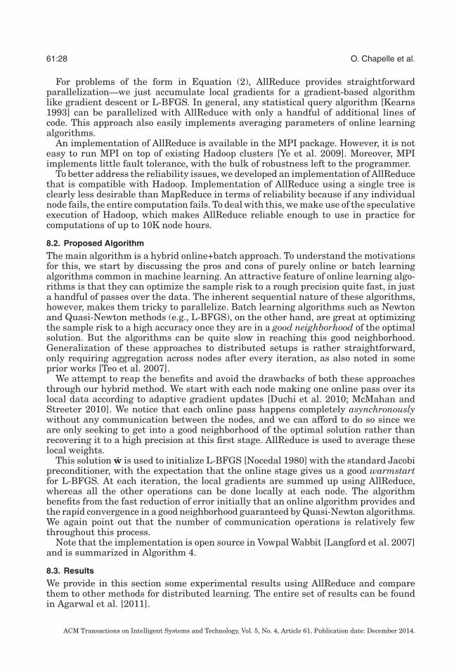
61:28 O. Chapelle et al.
For problems of the form in Equation (2), AllReduce provides straightforwardparallelization—we just accumulate local gradients for a gradient-based algorithmlike gradient descent or L-BFGS. In general, any statistical query algorithm [Kearns1993] can be parallelized with AllReduce with only a handful of additional lines ofcode. This approach also easily implements averaging parameters of online learningalgorithms.
An implementation of AllReduce is available in the MPI package. However, it is noteasy to run MPI on top of existing Hadoop clusters [Ye et al. 2009]. Moreover, MPIimplements little fault tolerance, with the bulk of robustness left to the programmer.
To better address the reliability issues, we developed an implementation of AllReducethat is compatible with Hadoop. Implementation of AllReduce using a single tree isclearly less desirable than MapReduce in terms of reliability because if any individualnode fails, the entire computation fails. To deal with this, we make use of the speculativeexecution of Hadoop, which makes AllReduce reliable enough to use in practice forcomputations of up to 10K node hours.
8.2. Proposed Algorithm
The main algorithm is a hybrid online+batch approach. To understand the motivationsfor this, we start by discussing the pros and cons of purely online or batch learningalgorithms common in machine learning. An attractive feature of online learning algo-rithms is that they can optimize the sample risk to a rough precision quite fast, in justa handful of passes over the data. The inherent sequential nature of these algorithms,however, makes them tricky to parallelize. Batch learning algorithms such as Newtonand Quasi-Newton methods (e.g., L-BFGS), on the other hand, are great at optimizingthe sample risk to a high accuracy once they are in a good neighborhood of the optimalsolution. But the algorithms can be quite slow in reaching this good neighborhood.Generalization of these approaches to distributed setups is rather straightforward,only requiring aggregation across nodes after every iteration, as also noted in someprior works [Teo et al. 2007].
We attempt to reap the benefits and avoid the drawbacks of both these approachesthrough our hybrid method. We start with each node making one online pass over itslocal data according to adaptive gradient updates [Duchi et al. 2010; McMahan andStreeter 2010]. We notice that each online pass happens completely asynchronouslywithout any communication between the nodes, and we can afford to do so since weare only seeking to get into a good neighborhood of the optimal solution rather thanrecovering it to a high precision at this first stage. AllReduce is used to average theselocal weights.
This solution w is used to initialize L-BFGS [Nocedal 1980] with the standard Jacobipreconditioner, with the expectation that the online stage gives us a good warmstartfor L-BFGS. At each iteration, the local gradients are summed up using AllReduce,whereas all the other operations can be done locally at each node. The algorithmbenefits from the fast reduction of error initially that an online algorithm provides andthe rapid convergence in a good neighborhood guaranteed by Quasi-Newton algorithms.We again point out that the number of communication operations is relatively fewthroughout this process.
Note that the implementation is open source in Vowpal Wabbit [Langford et al. 2007]and is summarized in Algorithm 4.
8.3. Results
We provide in this section some experimental results using AllReduce and comparethem to other methods for distributed learning. The entire set of results can be foundin Agarwal et al. [2011].
ACM Transactions on Intelligent Systems and Technology, Vol. 5, No. 4, Article 61, Publication date: December 2014.

Simple and Scalable Response Prediction for Display Advertising 61:29
Fig. 12. Speedup for obtaining a fixed test error relative to the run with 10 nodes, as a function of thenumber of nodes. The dashed line corresponds to the ideal speedup, the solid line is the average speedupover 10 repetitions, and the bars indicate maximum and minimal values.
ALGORITHM 4: Sketch of the Proposed Learning ArchitectureRequire: Data split across nodes
for all nodes k dowk = result on the data of node k using stochastic gradient descent.
end forCompute the average w using AllReduce.Start a preconditioned L-BFGS optimization from w.for t = 1, . . . , T do
for all nodes k doCompute gk the (local batch) gradient of examples on node kCompute g = ∑m
k=1 gk using AllReduce.Add the regularization part in the gradient.Take an L-BFGS step.
end forend for
8.3.1. Running Time. We study the running time as a function of the number of nodes.We varied the number of nodes from 10 to 100 and computed the speedup factor relativeto the run with 10 nodes. In each case, we measured the amount of time needed to get toa fixed test error. Since there can be significant variations from one run to the other—mostly because of the cluster utilization—each run was repeated 10 times. Results arereported in Figure 12. The speedup appears to be close to linear.
8.3.2. Online and Batch Learning. We investigate the number of iterations needed toreach a certain test performance for different learning strategies: batch, online, andhybrid.
Figure 13 compares two learning strategies—batch with and without an initial onlinepass—on the training set. It plots the optimality gap, defined as the difference betweenthe current objective function and the optimal one (i.e., minimum value of the objective,as in Equation (2)), as a function of the number iterations. From this figure, one cansee that the initial online pass results in a saving of about 10–15 iterations.
Figure 14 shows the test auPRC as a function of the number of iterations for four dif-ferent strategies: Only online learning, only L-BFGS learning, and two hybrid methods
ACM Transactions on Intelligent Systems and Technology, Vol. 5, No. 4, Article 61, Publication date: December 2014.
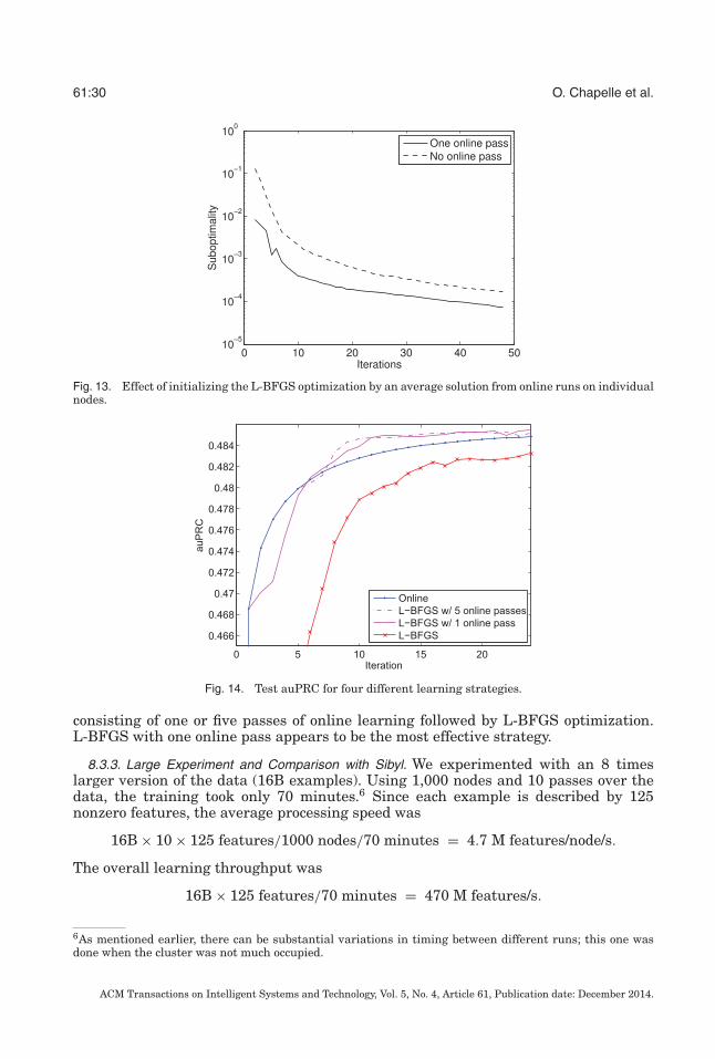
61:30 O. Chapelle et al.
Fig. 13. Effect of initializing the L-BFGS optimization by an average solution from online runs on individualnodes.
Fig. 14. Test auPRC for four different learning strategies.
consisting of one or five passes of online learning followed by L-BFGS optimization.L-BFGS with one online pass appears to be the most effective strategy.
8.3.3. Large Experiment and Comparison with Sibyl. We experimented with an 8 timeslarger version of the data (16B examples). Using 1,000 nodes and 10 passes over thedata, the training took only 70 minutes.6 Since each example is described by 125nonzero features, the average processing speed was
16B × 10 × 125 features/1000 nodes/70 minutes = 4.7 M features/node/s.
The overall learning throughput was
16B × 125 features/70 minutes = 470 M features/s.
6As mentioned earlier, there can be substantial variations in timing between different runs; this one wasdone when the cluster was not much occupied.
ACM Transactions on Intelligent Systems and Technology, Vol. 5, No. 4, Article 61, Publication date: December 2014.

Simple and Scalable Response Prediction for Display Advertising 61:31
Table IX. Average Training Time (in Seconds) per Iterationof an Internal Logistic Regression Implementation Using
Either MapReduce or AllReduce for Gradients Aggregation
Full size 10% sampleMapReduce 1690 1322AllReduce 670 59
We briefly compare this with a result reported for Sibyl for a run on 970 cores[Canini et al. 2012, slide 24]. The run was done over 129.1B examples, with 54.61nonzero features per example. The reported processing speed was 2.3M features/core/s(which is a factor of two slower than our achieved processing speed). The reportednumber of iterations is 10–50, which would lead to final learning throughput in therange of 45–223 M features/s (i.e., the results appear to be slower by a factor of 2–10).
8.4. Comparison with MapReduce
The standard way of using MapReduce for iterative machine learning algorithms isthe following [Chu et al. 2007]: Every iteration is an M/R job in which the mapperscompute some local statistics (such as a gradient) and the reducers sum them up. Thisis ineffective because each iteration has large overheads (job scheduling, data transfer,data parsing, etc.). We have an internal implementation of such a M/R algorithm. Weupdated this code to use AllReduce instead and compared both versions of the codein Table IX. This table confirms that Hadoop MapReduce has substantial overheadssince the training time is not much affected by the dataset size. The speedup factor ofAllReduce over Hadoop MapReduce can become extremely large for smaller datasetsand remains noticeable even for the largest datasets.
It is also noteworthy that all algorithms described in Chu et al. [2007] can be par-allelized with AllReduce, as well as further algorithms such as parameter averagingapproaches.
9. CONCLUSION
In this article, we presented a framework for modeling response prediction in displayadvertising. Our approach has several advantages over the alternatives:
—Simplicity. The proposed framework is easy to implement, trivial to update, andlightweight to use on real servers. The ad servers need only to load model filesthat can easily fit in memory and implement a model applier that uses only a hashfunction as feature generator.
—Scalability. Our algorithms are easy to parallelize. The map-reduce architecturepresented in this article allows us to train models using many billions of samples inone hour, a significant improvement over existing methods.
—Efficiency. The results presented in this article clearly show that our framework isas good as or better than the state-of-the-art alternatives.
The experiments reported in this study were conducted on data from two large (anddistinct) display advertising companies. The stability and repeatability of our resultssuggest strongly that the presented framework could serve as a strong baseline in thisdomain.
ACKNOWLEDGMENTS
We would like to thank our colleagues Kannan Achan, Haibin Cheng, Dmitry Pavlov, Benoıt Rostykus, andHuang Xu for providing us with valuable feedback, as well as for running some of the experiments in thispaper.
ACM Transactions on Intelligent Systems and Technology, Vol. 5, No. 4, Article 61, Publication date: December 2014.

61:32 O. Chapelle et al.
REFERENCES
A. Agarwal, O. Chapelle, M. Dudık, and J. Langford. 2011. A reliable effective terascale linear learningsystem. CoRR abs/1110.4198 (2011).
D. Agarwal, R. Agrawal, R. Khanna, and N. Kota. 2010. Estimating rates of rare events with multiplehierarchies through scalable log-linear models. In Proceedings of the 16th ACM SIGKDD InternationalConference on Knowledge Discovery and Data Mining. 213–222.
Azin Ashkan, Charles L. A. Clarke, Eugene Agichtein, and Qi Guo. 2009. Estimating ad clickthrough ratethrough query intent analysis. In Proceedings of the 2009 IEEE/WIC/ACM International Joint Confer-ence on Web Intelligence and Intelligent Agent Technology.
P. Auer, N. Cesa-Bianchi, and P. Fischer. 2002. Finite-time analysis of the multiarmed bandit problem.Machine Learning 47, 2 (2002), 235–256.
Francis Bach, Rodolphe Jenatton, Julien Mairal, and Guillaume Obozinski. 2011. Optimization with sparsity-inducing penalties. Foundations and Trends in Machine Learning 4, 1 (2011), 1–106.
Christopher M. Bishop. 2006. Pattern Recognition and Machine Learning. Springer-Verlag New York, Inc.B. H. Bloom. 1970. Space/time trade-offs in hash coding with allowable errors. Communications of the ACM
13, 7 (1970), 422–426.K. Canini, T. Chandra, E. Ie, J. McFadden, K. Goldman, M. Gunter, J. Harmsen, K. LeFevre, D. Lepikhin, T. L.
Llinares, I. Mukherjee, F. Pereira, J. Redstone, T. Shaked, and Y. Singer. 2012. Sibyl: A system for largescale supervised machine learning. (2012). Presentation at MLSS Santa Cruz, http://users.soe.ucsc.edu/niejiazhong/slides/chandra.pdf.
D. Chakrabarti, D. Agarwal, and V. Josifovski. 2008. Contextual advertising by combining relevance withclick feedback. In Proceedings of the 17th International Conference on World Wide Web. 417–426.
Yin-Wen Chang, Cho-Jui Hsieh, Kai-Wei Chang, Michael Ringgaard, and Chih-Jen Lin. 2010. Trainingand testing low-degree polynomial data mappings via linear SVM. The Journal of Machine LearningResearch 11 (2010), 1471–1490.
O. Chapelle and L. Li. 2011. An empirical evaluation of thompson sampling. In Advances in Neural Infor-mation Processing Systems 24, J. Shawe-Taylor, R. S. Zemel, P. Bartlett, F. C. N. Pereira, and K. Q.Weinberger (Eds.). 2249–2257.
S. F. Chen and J. Goodman. 1999. An empirical study of smoothing techniques for language modeling.Computer Speech & Language 13, 4 (1999), 359–393.
Haibin Cheng and Erick Cantu-Paz. 2010. Personalized click prediction in sponsored search. In Proceedingsof the 3rd ACM International Conference on Web Search and Data Mining. 351–360.
Haibin Cheng, Roelof van Zwol, Javad Azimi, Eren Manavoglu, Ruofei Zhang, Yang Zhou, and VidhyaNavalpakkam. 2012. Multimedia features for click prediction of new ads in display advertising. InProceedings of the 18th ACM SIGKDD International Conference on Knowledge Discovery and DataMining. 777–785.
C. T. Chu, S. K. Kim, Y. A. Lin, Y. Y. Yu, G. Bradski, A. Y. Ng, and K. Olukotun. 2007. Map-reduce formachine learning on multicore. In Proceedings of the 2006 Conference on Advances in Neural InformationProcessing Systems, Vol. 19.
Massimiliano Ciaramita, Vanessa Murdock, and Vassilis Plachouras. 2008. Online learning from click datafor sponsored search. In Proceedings of the 17th International Conference on World Wide Web. 227–236.
C. Cortes, Y. Mansour, and M. Mohri. 2010. Learning bounds for importance weighting. In Advances inNeural Information Processing Systems, Vol. 23. 442–450.
Jeffrey Dean and Sanjay Ghemawat. 2008. MapReduce: Simplified data processing on large clusters. Com-mun. ACM 51, 1 (2008), 107–113.
John Duchi, Elad Hazan, and Yoram Singer. 2010. Adaptive subgradient methods for online learning andstochastic optimization. Journal of Machine Learning Research 12 (2010), 2121–2159.
Theodoros Evgeniou and Massimiliano Pontil. 2004. Regularized multi-task learning. In Proceedings of the10th ACM SIGKDD International Conference on Knowledge Discovery and Data Mining. ACM, 109–117.
A. Gelman and J. Hill. 2006. Data Analysis Using Regression and Multilevel/Hierarchical Models. CambridgeUniversity Press.
John C. Gittins. 1989. Multi-armed Bandit Allocation Indices. John Wiley & Sons.T. Graepel, J. Quinonero Candela, T. Borchert, and R. Herbrich. 2010. Web-scale Bayesian click-through rate
prediction for sponsored search advertising in Microsoft’s bing search engine. In Proceedings of the 27thInternational Conference on Machine Learning. 13–20.
I. Guyon and A. Elisseeff. 2003. An introduction to variable and feature selection. The Journal of MachineLearning Research 3 (2003), 1157–1182.
ACM Transactions on Intelligent Systems and Technology, Vol. 5, No. 4, Article 61, Publication date: December 2014.

Simple and Scalable Response Prediction for Display Advertising 61:33
D. Hillard, E. Manavoglu, H. Raghavan, C. Leggetter, E. Cantu-Paz, and R. Iyer. 2011. The sum of its parts:Reducing sparsity in click estimation with query segments. Information Retrieval (2011), 1–22.
D. Hillard, S. Schroedl, E. Manavoglu, H. Raghavan, and C. Leggetter. 2010. Improving ad relevance insponsored search. In Proceedings of the 3rd ACM International Conference on Web Search and DataMining. 361–370.
Michael Kearns. 1993. Efficient noise-tolerant learning from statistical queries. In Proceedings of the 25thAnnual ACM Symposium on the Theory of Computing. 392–401.
G. King and L. Zeng. 2001. Logistic regression in rare events data. Political Analysis 9, 2 (2001), 137–163.H. Koepke and M. Bilenko. 2012. Fast prediction of new feature utility. In Proceedings of the 29th Interna-
tional Conference on Machine Learning. 791–798.Nagaraj Kota and Deepak Agarwal. 2011. Temporal multi-hierarchy smoothing for estimating rates of rare
events. In Proceedings of the 17th ACM SIGKDD International Conference on Knowledge Discovery andData Mining. 1361–1369.
T. L. Lai and H. Robbins. 1985. Asymptotically efficient adaptive allocation rules. Advances in AppliedMathematics 6 (1985), 4–22.
J. Langford, L. Li, and A. Strehl. 2007. Vowpal Wabbit Open Source Project. https://github.com/JohnLangford/vowpal_wabbit/wiki. (2007).
L. Li, W. Chu, J. Langford, and R. E. Schapire. 2010. A contextual-bandit approach to personalized newsarticle recommendation. In Proceedings of the 19th International Conference on World Wide Web. 661–670.
L. Li, W. Chu, J. Langford, and X. Wang. 2011. Unbiased offline evaluation of contextual-bandit-based newsarticle recommendation algorithms. In Proceedings of the 4th ACM International Conference on WebSearch and Data Mining. 297–306.
Yandong Liu, Sandeep Pandey, Deepak Agarwal, and Vanja Josifovski. 2012. Finding the right consumer:Optimizing for conversion in display advertising campaigns. In Proceedings of the 5th ACM InternationalConference on Web Search and Data Mining. 473–482.
Yucheng Low, Joseph Gonzalez, Aapo Kyrola, Danny Bickson, Carlos Guestrin, and Joseph M. Hellerstein.2010. GraphLab: A new framework for parallel machine learning. In The 26th Conference on Uncertaintyin Artificial Intelligence.
James MacQueen. 1967. Some methods for classification and analysis of multivariate observations. In Pro-ceedings of 5th Berkeley Symposium on Mathematical Statistics and Probability. University of CaliforniaPress, Berkeley, CA, 281–297.
R. P. McAfee. 2011. The design of advertising exchanges. Review of Industrial Organization (2011), 1–17.H. B. McMahan and M. Streeter. 2010. Adaptive bound optimization for online convex optimization. In
Proceedings of the 23rd Annual Conference on Learning Theory. 244–256.C. Meek, D. M. Chickering, and D. Wilson. 2005. Stochastic and contingent payment auctions. In Workshop
on Sponsored Search Auctions, ACM Electronic Commerce.Lukas Meier, Sara Van De Geer, and Peter Buhlmann. 2008. The group lasso for logistic regression. Journal
of the Royal Statistical Society: Series B (Statistical Methodology) 70, 1 (2008), 53–71.S. Menard. 2001. Applied Logistic Regression Analysis. Vol. 106. Sage Publications, Inc.Aditya Krishna Menon, Krishna-Prasad Chitrapura, Sachin Garg, Deepak Agarwal, and Nagaraj Kota. 2011.
Response prediction using collaborative filtering with hierarchies and side-information. In Proceedingsof the 17th ACM SIGKDD International Conference on Knowledge Discovery and Data Mining. 141–149.
T. P. Minka. 2003. A Comparison of Numerical Optimizers for Logistic Regression. Technical Report. MicrosoftResearch. Retrieved from http://research.microsoft.com/en-us/um/people/minka/papers/logreg/.
S. Muthukrishnan. 2009. Ad exchanges: Research issues. In Proceedings of the 5th International Workshopon Internet and Network Economics. 1–12.
K. Nigam, J. Lafferty, and A. McCallum. 1999. Using maximum entropy for text classification. In IJCAI-99Workshop on Machine Learning for Information Filtering, Vol. 1. 61–67.
J. Nocedal. 1980. Updating quasi-Newton matrices with limited storage. Mathematics of Computation 35,151 (1980), 773–782.
A. B. Owen. 2007. Infinitely imbalanced logistic regression. The Journal of Machine Learning Research 8(2007), 761–773.
Moira Regelson and Daniel C. Fain. 2006. Predicting click-through rate using keyword clusters. In Proceed-ings of the Second Workshop on Sponsored Search Auctions.
ACM Transactions on Intelligent Systems and Technology, Vol. 5, No. 4, Article 61, Publication date: December 2014.

61:34 O. Chapelle et al.
M. Richardson, E. Dominowska, and R. Ragno. 2007. Predicting clicks: Estimating the click-through ratefor new ads. In Proceedings of the 16th International Conference on World Wide Web. New York, NY,521–530.
R. Rosales and O. Chapelle. 2011. Attribute selection by measuring information on reference distri-butions. In Tech Pulse Conference, Yahoo!. Retrieved from http://people.csail.mit.edu/romer/papers/RosChaTP11.pdf.
R. Rosales, H. Cheng, and E. Manavoglu. 2012. Post-click conversion modeling and analysis for non-guaranteed delivery display advertising. In Proceedings of the 5th ACM International Conference onWeb Search and Data Mining. ACM, 293–302.
J. Sarkar. 1991. One-armed bandit problems with covariates. The Annals of Statistics (1991), 1978–2002.B. Scholkopf and A. J. Smola. 2001. Learning with Kernels: Support Vector Machines, Regularization, Opti-
mization, and Beyond. MIT Press.Q. Shi, J. Petterson, G. Dror, J. Langford, A. Smola, and SVN Vishwanathan. 2009. Hash kernels for struc-
tured data. The Journal of Machine Learning Research 10 (2009), 2615–2637.C. Teo, Q. Le, A. Smola, and SVN Vishwanathan. 2007. A scalable modular convex solver for regularized
risk minimization. In Proceedings of the 13th ACM SIGKDD International Conference on KnowledgeDiscovery and Data Mining. 727–736.
William R. Thompson. 1933. On the likelihood that one unknown probability exceeds another in view of theevidence of two samples. Biometrika 25, 3–4 (1933), 285–294.
K. Weinberger, A. Dasgupta, J. Langford, A. Smola, and J. Attenberg. 2009. Feature hashing for large scalemultitask learning. In Proceedings of the 26th Annual International Conference on Machine Learning.1113–1120.
Jerry Ye, Jyh-Herng Chow, Jiang Chen, and Zhaohui Zheng. 2009. Stochastic gradient boosted distributeddecision trees. In Proceeding of the 18th ACM Conference on Information and Knowledge Management.2061–2064.
Matei Zaharia, Mosharaf Chowdhury, Tathagata Das, Ankur Dave, Justin Ma, Murphy McCauley, MichaelFranklin, Scott Shenker, and Ion Stoica. 2012. Resilient distributed datasets: A fault-tolerant abstractionfor in-memory cluster computing. In Proceedings of the 9th USENIX Conference on Networked SystemsDesign and Implementation. 15–28.
Received December 2012; revised April 2013; accepted August 2013
ACM Transactions on Intelligent Systems and Technology, Vol. 5, No. 4, Article 61, Publication date: December 2014.