Simple and Robust Risk Budgeting Using TEES

Thomas K. Philips

Regional Head of Investment Risk and Performance

BNP Paribas Investment Partners

This presentation may not be reproduced or redistributed, in any form and by any means, without the prior written consent of

Fischer Francis Trees & Watts, Inc. Opinions expressed are current as of the date appearing in this document only.

I. How I learned to stop worrying and start loving risk budgeting

II. Coherent risk measures: A better way to think about risk

III. Simple and robust risk budgeting using TEES

IV. A real-life example of a robust risk budget

Agenda

2

V. Summary and open questions

VI. Appendices

I. Better coherent measures of tail risk

II. A robust estimator of average correlation

III. Univariate OLS revisited and Theil-Sen regression

IV. Using robust regression to derive robust estimates of correlation

V. Estimating robust correlation and covariance matrices

Risk Budgeting is Portfolio Optimization by Another Name

● I got interested in risk budgeting when it entered our investment process after a merger

– Risk Budget = vol contribution of a strategy we want to include in our portfolio =

● Basic problem setup

– CIO / product head has high level views on asset classes, alpha teams and strategies

– Views on individual assets typically reside with a specialist

iix σ×

3

● We need to solve a two level allocation / optimization problem

– CIO / Product head optimally allocates risk to alpha teams and strategies

– Alpha teams allocate active risk between individual securities and sub-strategies

● In this context, risk budgeting feels more natural than portfolio optimization

– But risk budgeting is most often done in a mean-variance framework

– And fixed income is loaded with tail risk, both explicit (options) and implicit (credit, liquidity)

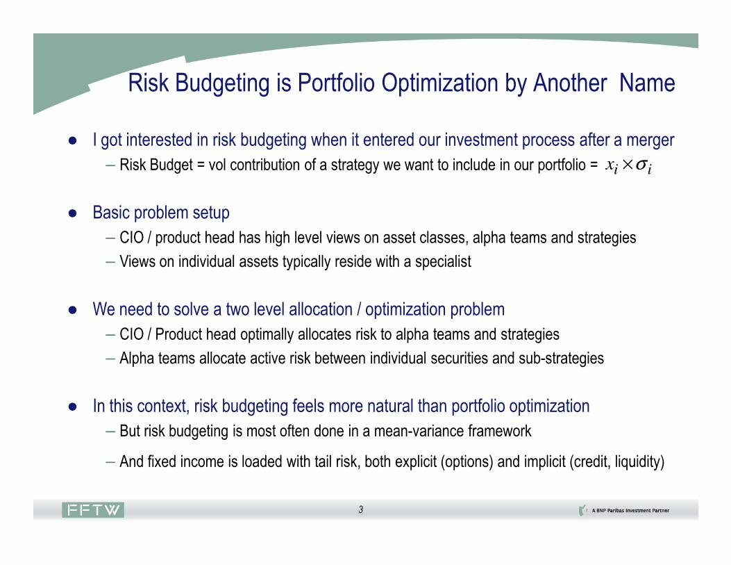
Tail Risk: Short Term Corporates vs. Treasuries

4

Source: Merrill Lynch MLX Global Index System and BNP Paribas Investment Partners

Cum. Excess Return: Short Term Corporates vs. Treasuries

5

Source: BNP Paribas Investment Partners

Risk Budgeting – Needs, Wants and What’s Available

● I needed to create risk budgets in a user friendly and computationally tractable way

– Account for tail risk in an intuitive way without requiring a huge infrastructure

– OK to work at strategy level, no need to drill down to individual securities

● None of the traditional enhanced Mean-Variance approaches met my needs

– Resampling (Michaud and Michaud)

– Shrinkage (Jobson and Korkie, Ledoit and Wolf)

6

– Shrinkage (Jobson and Korkie, Ledoit and Wolf)

– Direct estimation of the utility function via simulation (Sharpe)

– Robust optimization (Ceria)

– Black-Litterman (Black and Litterman)

● ETL Optimization (Rachev and Martin) met many of my needs but was too complex

● My requirements practically mandated a different approach

– First need to define exactly how we want to think about risk

Redefining Risk: Artzner, Delbaen, Eber, Heath, 1997

● Risk is synonymous with loss – it’s not the same as uncertainty in return

– Risk is a measure of the amount of cash needed to support a position / a strategy / a portfolio

● A good risk measure for an asset / a strategy / a portfolio X satisfies these axioms

– Relevance: If Return (X) is sometimes < 0 , then Risk (X) > 0

– Monotonicity: If Return (X) is almost surely <= Return (Y), then Risk (X) >= Risk (Y)

– Positive Homogeneity: Risk (c*X) = c * Risk (X)

7

– Positive Homogeneity: Risk (c*X) = c * Risk (X)

– Translation Invariance: Risk (X + cash) = Risk (X) – cash

– Subadditivity: Risk (X + Y) <= Risk (X) + Risk (Y)

● A risk measure that satisfies these criteria is called a coherent measure of risk

– Standard deviation is not coherent (Does not satisfy monotonicity)

– VaR is not coherent (Does not satisfy subadditivity)

– Expected Shortfall is coherent (Satisfies all the axioms)

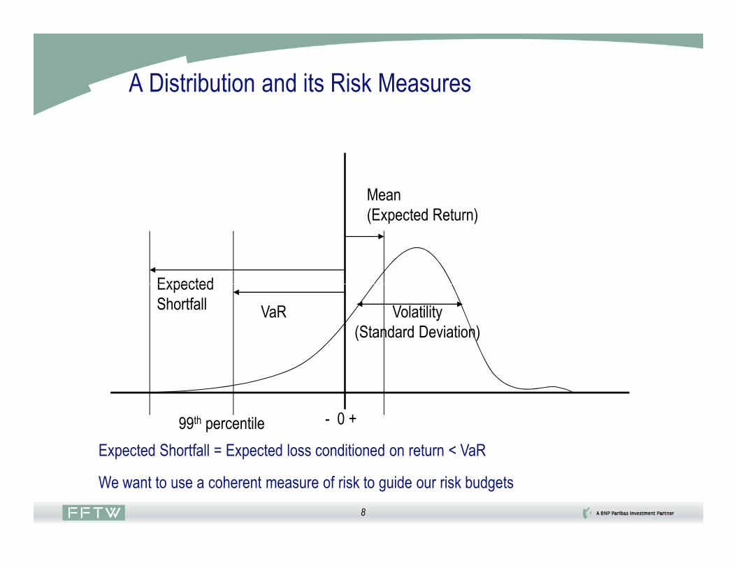
A Distribution and its Risk Measures

Expected

Mean

(Expected Return)

8

VaR

Expected

Shortfall

- 0 +99th percentile

Volatility

(Standard Deviation)

Expected Shortfall = Expected loss conditioned on return < VaR

We want to use a coherent measure of risk to guide our risk budgets

Review: MV Risk Budgeting With Independent Alpha Sources

● Blitz and Hottinga: assume we have a beta portfolio and N alpha portfolios

– The alpha portfolios are independent of the beta portfolio and of each other

– The ith alpha portfolio has an information ratio of IRi

● How should we budget our risk to achieve a tracking error of TETarget?

● Blitz and Hottinga solve Markowitz’s mean variance equations to get

9

● Blitz and Hottinga solve Markowitz’s mean variance equations to get

● Risk budgets depend only on relative Information Ratios and Target TE!

● Important special case: If all IR’s are equal, all risk budgets are equal to

Target22

2

2

1

TEIRIRIR

IRBudgetRisk

N

ii ×

+++=

L

N

TETarget

Risk Budgeting With Independent Alpha Sources: Example

1005.0

×

● Simple example: 2 alpha sources, each with an IR of 1, TETarget= 100 bp

– Risk budget for alpha source 1 = = 71 bp

– Risk budget for alpha source 2 = = 71 bp

● What if the information ratios were 0.5 and not 1?

10011

1

22×

+

10011

1

22×

+

10

1005.05.0

5.0

22×

+

1005.05.0

5.0

22×

+

10015.0

5.0

22×

+

– Risk budget for alpha source 1 = = 71 bp

– Risk budget for alpha source 2 = = 71 bp

● Change the information ratios to 0.5 and 1. What happens now?

– Risk budget for alpha source 1 = = 45 bp

– Risk budget for alpha source 2 = = 89 bp

10015.0

1

22×

+

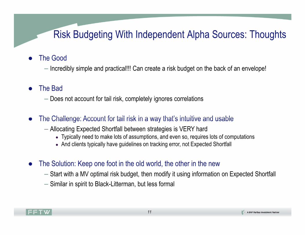
Risk Budgeting With Independent Alpha Sources: Thoughts

● The Good

– Incredibly simple and practical!!! Can create a risk budget on the back of an envelope!

● The Bad

– Does not account for tail risk, completely ignores correlations

● The Challenge: Account for tail risk in a way that’s intuitive and usable

11

● The Challenge: Account for tail risk in a way that’s intuitive and usable

– Allocating Expected Shortfall between strategies is VERY hard● Typically need to make lots of assumptions, and even so, requires lots of computations

● And clients typically have guidelines on tracking error, not Expected Shortfall

● The Solution: Keep one foot in the old world, the other in the new

– Start with a MV optimal risk budget, then modify it using information on Expected Shortfall

– Similar in spirit to Black-Litterman, but less formal

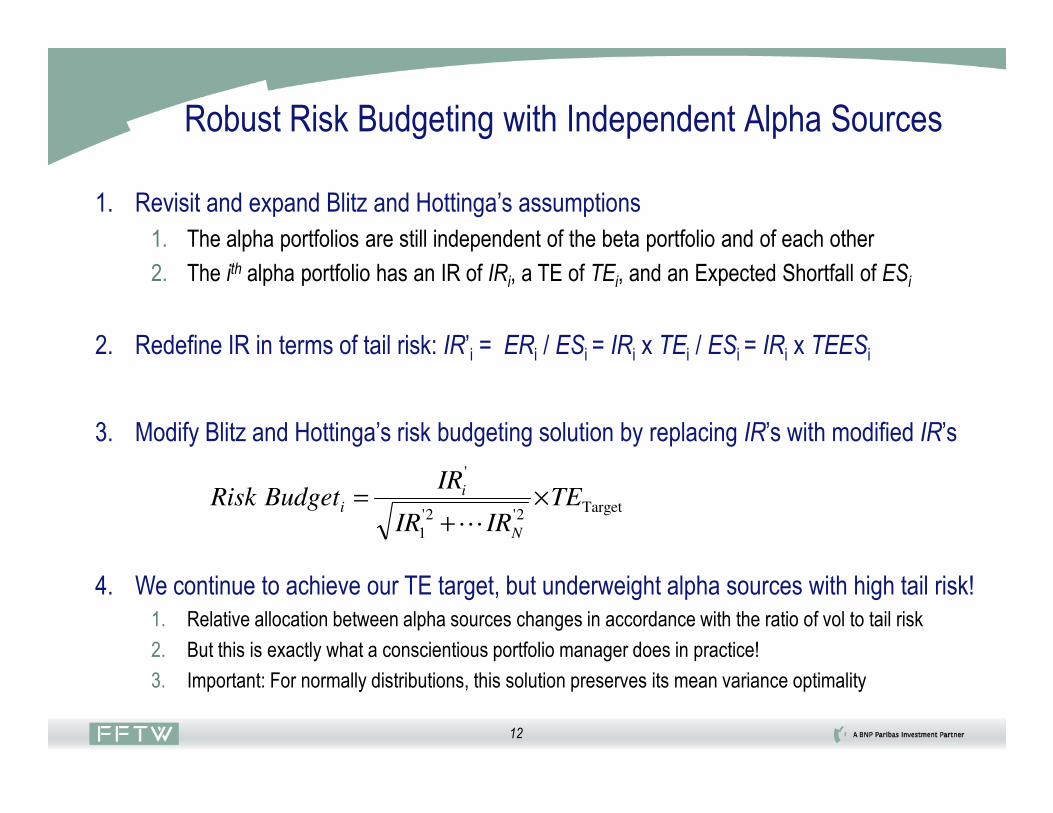
Robust Risk Budgeting with Independent Alpha Sources

1. Revisit and expand Blitz and Hottinga’s assumptions

1. The alpha portfolios are still independent of the beta portfolio and of each other

2. The ith alpha portfolio has an IR of IRi, a TE of TEi, and an Expected Shortfall of ESi

2. Redefine IR in terms of tail risk: IR’i = ERi / ESi = IRi x TEi / ESi = IRi x TEESi

12

3. Modify Blitz and Hottinga’s risk budgeting solution by replacing IR’s with modified IR’s

4. We continue to achieve our TE target, but underweight alpha sources with high tail risk!

1. Relative allocation between alpha sources changes in accordance with the ratio of vol to tail risk

2. But this is exactly what a conscientious portfolio manager does in practice!

3. Important: For normally distributions, this solution preserves its mean variance optimality

Target2'2'

1

'

TEIRIR

IRBudgetRisk

N

ii ×

+=

L

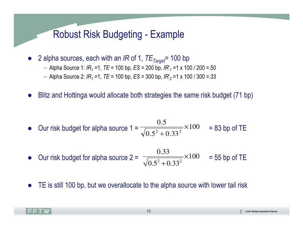
Robust Risk Budgeting - Example

● 2 alpha sources, each with an IR of 1, TETarget= 100 bp

– Alpha Source 1: IR1 =1, TE = 100 bp, ES = 200 bp, IR’1 =1 x 100 / 200 =.50

– Alpha Source 2: IR1 =1, TE = 100 bp, ES = 300 bp, IR’2 =1 x 100 / 300 =.33

● Blitz and Hottinga would allocate both strategies the same risk budget (71 bp)

13

● Our risk budget for alpha source 1 = = 83 bp of TE

● Our risk budget for alpha source 2 = = 55 bp of TE

● TE is still 100 bp, but we overallocate to the alpha source with lower tail risk

10033.05.0

5.0

22×

+

10033.05.0

33.0

22×

+

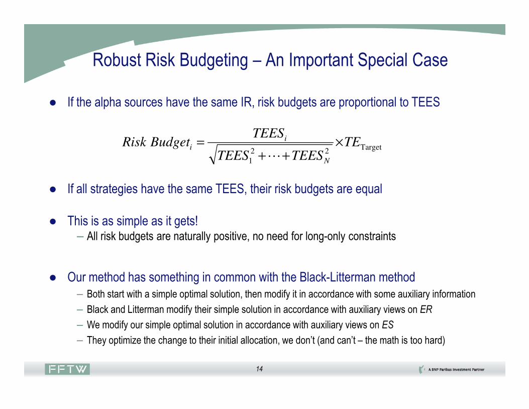
Robust Risk Budgeting – An Important Special Case

● If the alpha sources have the same IR, risk budgets are proportional to TEES

● If all strategies have the same TEES, their risk budgets are equal

Target22

1

TETEESTEES

TEESBudgetRisk

N

ii ×

++=

L

14

● This is as simple as it gets!– All risk budgets are naturally positive, no need for long-only constraints

● Our method has something in common with the Black-Litterman method

– Both start with a simple optimal solution, then modify it in accordance with some auxiliary information

– Black and Litterman modify their simple solution in accordance with auxiliary views on ER

– We modify our simple optimal solution in accordance with auxiliary views on ES

– They optimize the change to their initial allocation, we don’t (and can’t – the math is too hard)

Dealing With Correlations

● Berkelaar, Kobor and Tsumagiri: risk budgeting for correlated alpha sources

● Have to invert the correlation matrix, cannot guarantee positive risk budgets

[ ] [ ] [ ][ ][ ] [ ] [ ]

Target1

1

TEIRIR

IRBudgetRisk

T

ii

×=−

−

ρ

ρ

15

● Some pragmatic choices result in positive robust risk budgets with correlated alphas

– Shrink correlation matrix, replace individual correlations by average correlation● Elton and Gruber (1973), Elton, Gruber and Urich (1978)

– Replace all IRs by modified IRs

[ ][ ] [ ][ ]

[ ] [ ] [ ]Target

1

1

''

' TE

IRIR

IRBudgetRisk

AverageT

iAverage

i ×=−

−

ρ

ρ

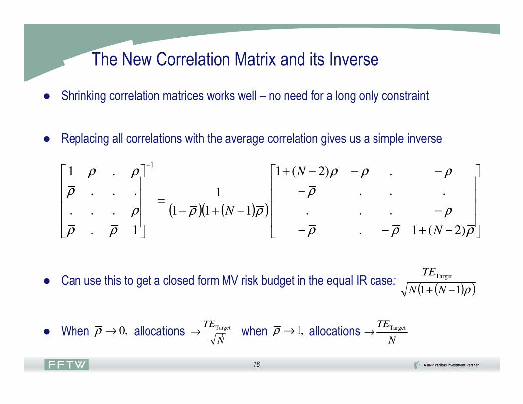
The New Correlation Matrix and its Inverse

( ) ( )( )

−

−

−−−+

−+−=

−

ρ

ρ

ρρρ

ρρρ

ρ

ρρ

...

.)2(1

1...

.11

N

● Shrinking correlation matrices works well – no need for a long only constraint

● Replacing all correlations with the average correlation gives us a simple inverse

16

,0→ρ

( ) ( )( )

−+−−

−−+−=

ρρρ

ρρρ

ρρ

ρ

)2(1.

...111

1.

...

N

N

,1→ρ

● Can use this to get a closed form MV risk budget in the equal IR case:

● When allocations , when allocations N

TETarget→

N

TETarget→

( )( )ρ11

Target

−+ NN

TE

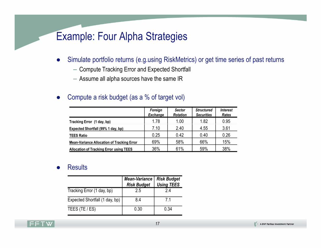
Example: Four Alpha Strategies

● Simulate portfolio returns (e.g.using RiskMetrics) or get time series of past returns

– Compute Tracking Error and Expected Shortfall

– Assume all alpha sources have the same IR

● Compute a risk budget (as a % of target vol)

Foreign

Exchange

Sector

Rotation

Structured

Securities

Interest

Rates

Tracking Error (1 day, bp) 1.78 1.00 1.82 0.95

17

● Results

Expected Shortfall (99% 1 day, bp) 7.10 2.40 4.55 3.61

TEES Ratio 0.25 0.42 0.40 0.26

Mean-Variance Allocation of Tracking Error 69% 58% 66% 15%

Allocation of Tracking Error using TEES 36% 61% 59% 38%

Mean-Variance

Risk Budget

Risk Budget

Using TEES

Tracking Error (1 day, bp) 2.5 2.4

Expected Shortfall (1 day, bp) 8.4 7.1

TEES (TE / ES) 0.30 0.34

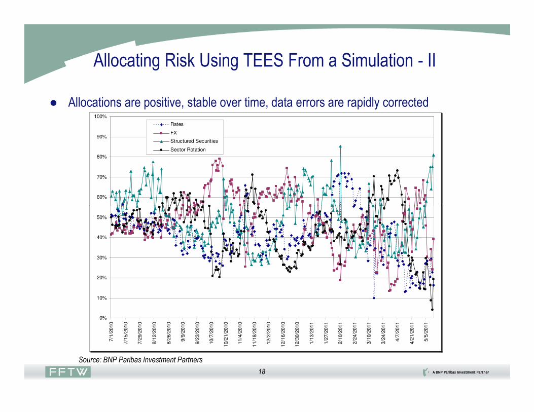
Allocating Risk Using TEES From a Simulation - II

● Allocations are positive, stable over time, data errors are rapidly corrected

60%

70%

80%

90%

100%

Rates

FX

Structured Securities

Sector Rotation

18

0%

10%

20%

30%

40%

50%

7/1

/2010

7/1

5/2

010

7/2

9/2

010

8/1

2/2

010

8/2

6/2

010

9/9

/2010

9/2

3/2

010

10/7

/2010

10/2

1/2

010

11/4

/2010

11/1

8/2

010

12/2

/2010

12/1

6/2

010

12/3

0/2

010

1/1

3/2

011

1/2

7/2

011

2/1

0/2

011

2/2

4/2

011

3/1

0/2

011

3/2

4/2

011

4/7

/2011

4/2

1/2

011

5/5

/2011

Source: BNP Paribas Investment Partners

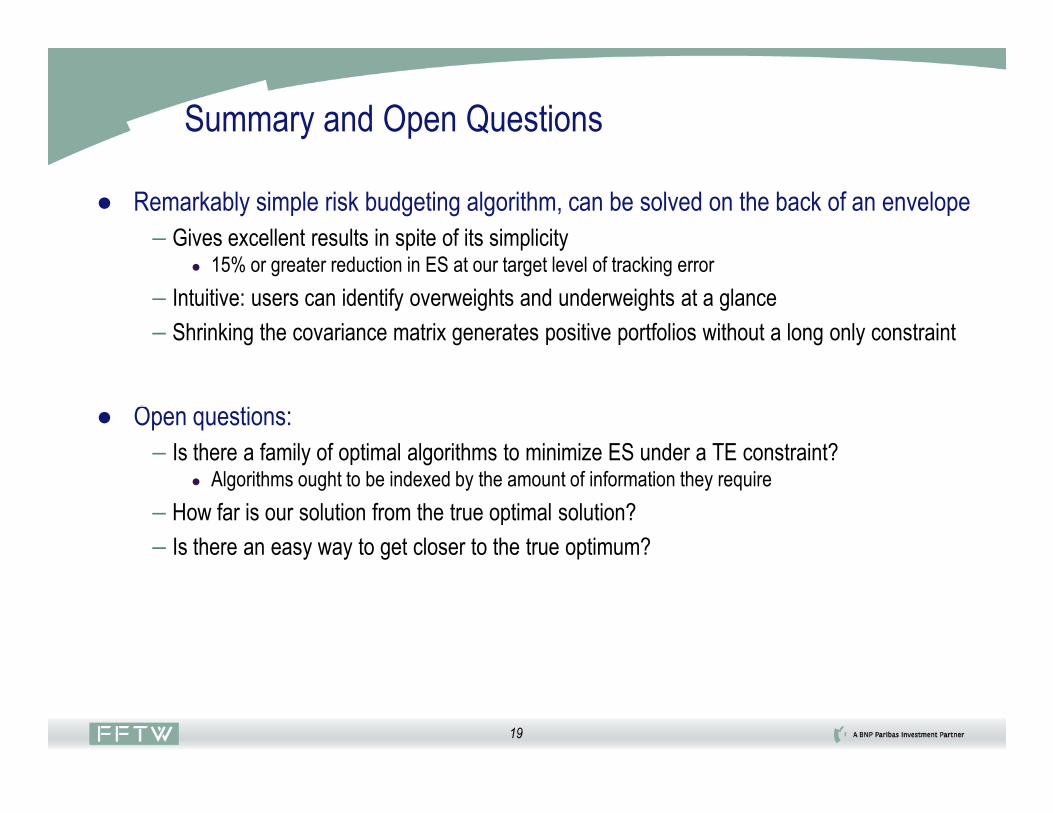
Summary and Open Questions

● Remarkably simple risk budgeting algorithm, can be solved on the back of an envelope

– Gives excellent results in spite of its simplicity● 15% or greater reduction in ES at our target level of tracking error

– Intuitive: users can identify overweights and underweights at a glance

– Shrinking the covariance matrix generates positive portfolios without a long only constraint

● Open questions:

19

● Open questions:

– Is there a family of optimal algorithms to minimize ES under a TE constraint?● Algorithms ought to be indexed by the amount of information they require

– How far is our solution from the true optimal solution?

– Is there an easy way to get closer to the true optimum?

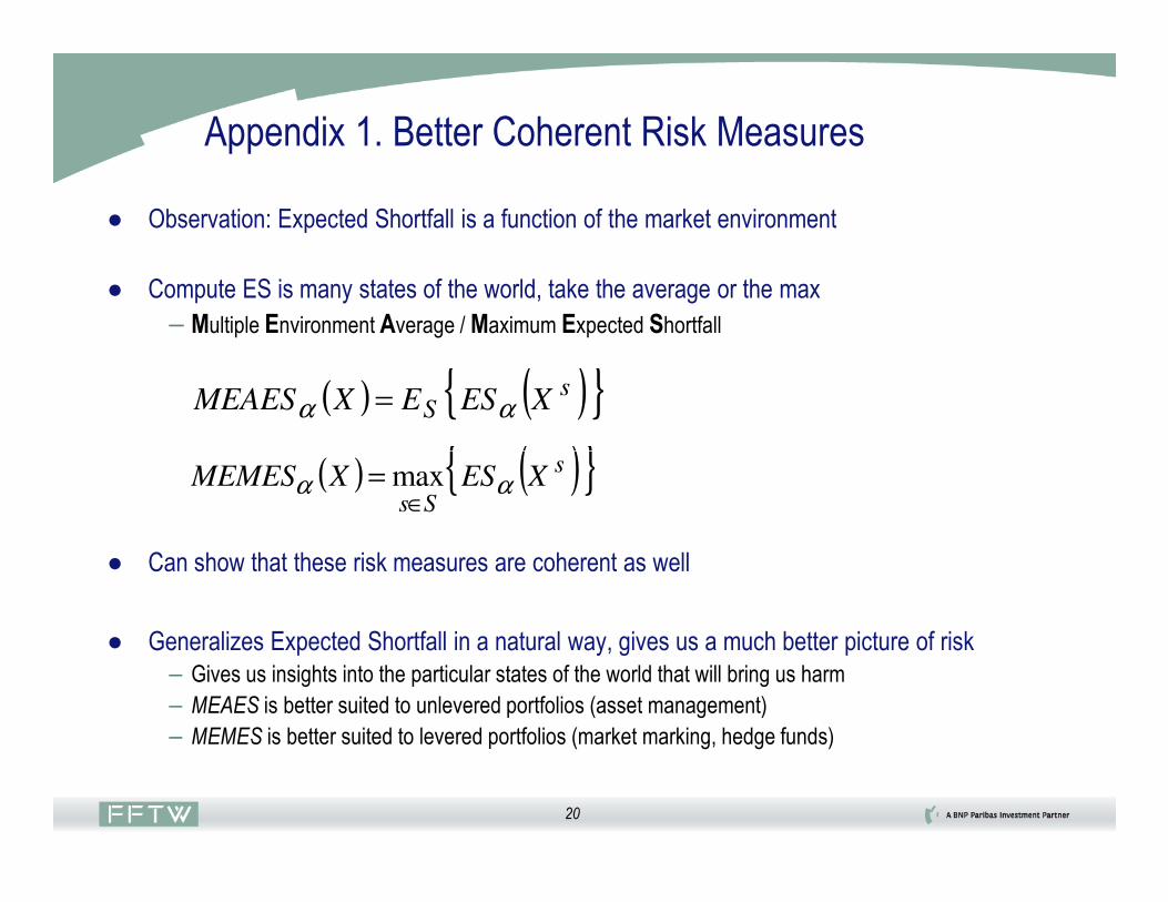
Appendix 1. Better Coherent Risk Measures

● Observation: Expected Shortfall is a function of the market environment

● Compute ES is many states of the world, take the average or the max

– Multiple Environment Average / Maximum Expected Shortfall

( ) ( ){ } sS XESEXMEAES αα =

( ) ( ){ }s

20

● Can show that these risk measures are coherent as well

● Generalizes Expected Shortfall in a natural way, gives us a much better picture of risk

– Gives us insights into the particular states of the world that will bring us harm

– MEAES is better suited to unlevered portfolios (asset management)

– MEMES is better suited to levered portfolios (market marking, hedge funds)

( ) ( ){ } max s

SsXESXMEMES αα

∈=

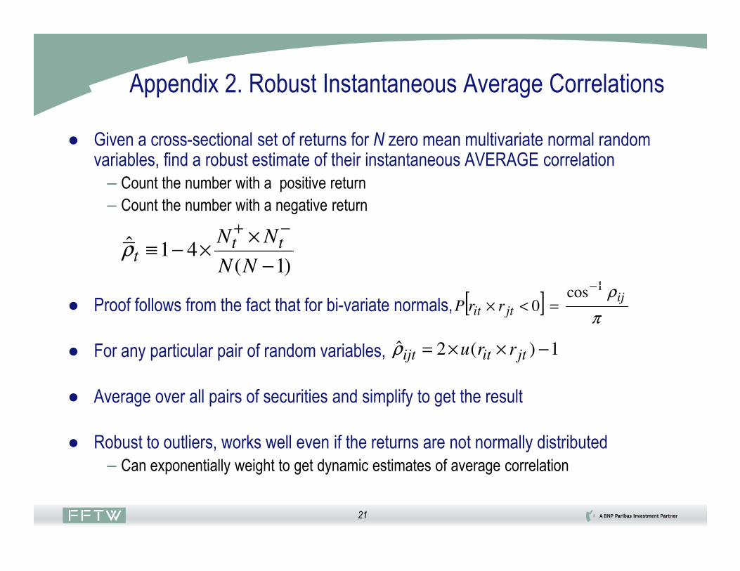
Appendix 2. Robust Instantaneous Average Correlations

● Given a cross-sectional set of returns for N zero mean multivariate normal random variables, find a robust estimate of their instantaneous AVERAGE correlation

– Count the number with a positive return

– Count the number with a negative return

)1(41ˆ

−

××−≡

−+

NN

NN tttρ

[ ] ρ1cos−

21

● Proof follows from the fact that for bi-variate normals,

● For any particular pair of random variables,

● Average over all pairs of securities and simplify to get the result

● Robust to outliers, works well even if the returns are not normally distributed

– Can exponentially weight to get dynamic estimates of average correlation

[ ]π

ρijjtit rrP

1cos 0

−

=<×

1)(2ˆ −××= jtitijt rruρ

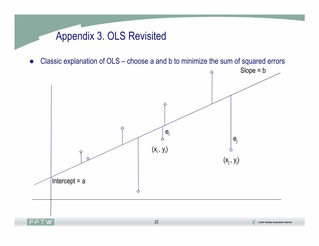
Appendix 3. OLS Revisited

● Classic explanation of OLS – choose a and b to minimize the sum of squared errorsSlope = b

22

ei

Intercept = a

ej

(xi , yi)

(xj , yj)

Appendix 3. OLS Revisited

● A different explanation of OLS – form a weighted average of all possible slopes

Intercept = aij

Slope = b

OLS Intercept = a = weighted average of all the aij!

OLS Slope = b = weighted average of all the bij! ( )

( )∑∑

∑∑

−

−

=

ji

i j

ijji

xx

bxx

b2

2

23

( )

( )∑∑

∑∑

−

−

=

i j

ji

i j

ijji

xx

axx

a2

2

(xi , yi)

(xj , yj)

Slope = bij

∑∑i j

ji

Appendix 3. The Theil-Sen Estimator

● Theil-Sen robust estimate of slope = median of all N(N-1)/2 slopes (i.e. the bij’s)

● Theil-Sen intercept chosen to make the median error 0

● Incredibly robust to outliers, works well even if the returns are not normally distributed

– Approximately 25% of the points can be arbitrarily bad before it stops working

24

– OLS, in contrast can be corrupted by a single outlier

– Sum of squared errors is always within 10% or so of OLS

● In the univariate case, Theil-Sen should replace OLS universally

– Not a good choice for multivariate regression – Theil Sen can converge to the wrong answer● Particularly true if the relationship is nonlinear

– But there are other robust regression algorithms that work well with multivariate data

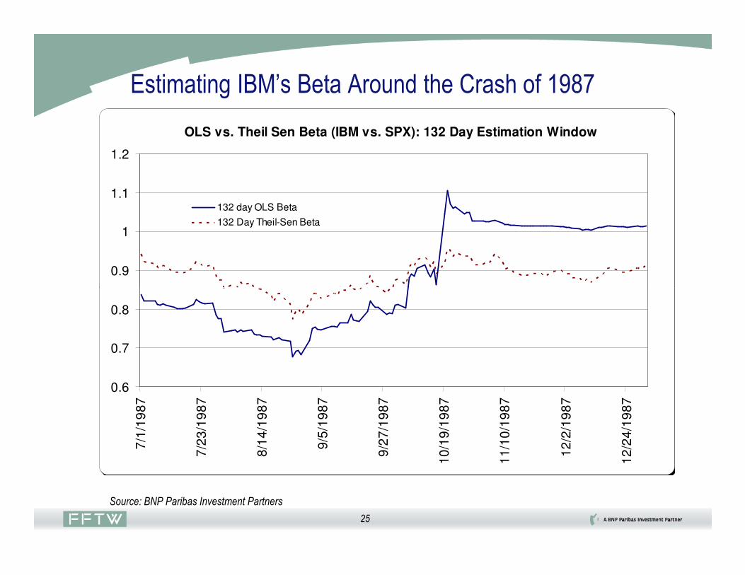
Estimating IBM’s Beta Around the Crash of 1987

OLS vs. Theil Sen Beta (IBM vs. SPX): 132 Day Estimation Window

0.9

1

1.1

1.2

132 day OLS Beta

132 Day Theil-Sen Beta

25

0.6

0.7

0.8

7/1

/19

87

7/2

3/1

98

7

8/1

4/1

98

7

9/5

/19

87

9/2

7/1

98

7

10

/19

/19

87

11

/10

/19

87

12

/2/1

98

7

12

/24

/19

87

Source: BNP Paribas Investment Partners

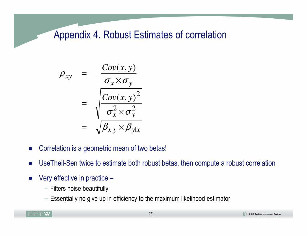
Appendix 4. Robust Estimates of correlation

yx

yxxy

yxCov

yxCov

22

2),(

),(

σσ

σσρ

×=

×=

26

● Correlation is a geometric mean of two betas!

● UseTheil-Sen twice to estimate both robust betas, then compute a robust correlation

● Very effective in practice –

– Filters noise beautifully

– Essentially no give up in efficiency to the maximum likelihood estimator

xyyx || ββ ×=

Simulations With Independent Random Variables

Percentiles 1 5 10 25 50 75 90 95 99

Theil Sen Slope -0.26 -0.17 -0.14 -0.07 0 0.07 0.13 0.18 0.26

Least Squares Slope -0.24 -0.17 -0.13 -0.07 0 0.07 0.13 0.17 0.24

Theil Sen Intercept -0.3 -0.21 -0.16 -0.09 0 0.08 0.16 0.21 0.3

Least Squares Intercept -0.23 -0.17 -0.13 -0.07 0 0.07 0.13 0.17 0.23

Theil Sen Mean Square Error 0.69 0.77 0.81 0.89 0.98 1.08 1.17 1.24 1.35

Least Squares Mean Square Error 0.69 0.76 0.81 0.88 0.98 1.07 1.16 1.23 1.33

Theil Sen Median Error 0 0 0 0 0 0 0 0 0

Least Squares Median Error -0.17 -0.12 -0.09 -0.05 0 0.05 0.09 0.12 0.18

Theil Sen correlation -0.24 -0.17 -0.14 -0.07 0 0.07 0.13 0.18 0.25

Least Squares correlation -0.23 -0.17 -0.13 -0.07 0 0.07 0.13 0.16 0.23

Distribution= Normal(0,1), N=100

27

Percentiles 1 5 10 25 50 75 90 95 99

Theil Sen Slope -0.12 -0.07 -0.05 -0.03 0 0.03 0.06 0.09 0.14

Least Squares Slope -0.35 -0.18 -0.13 -0.07 -0.02 0.03 0.13 0.23 0.65

Theil Sen Intercept 1.17 1.24 1.28 1.34 1.41 1.49 1.57 1.62 1.74

Least Squares Intercept 0.98 1.49 1.62 1.78 1.95 2.16 2.41 2.62 3.44

Theil Sen Mean Square Error 0.59 0.88 1.11 1.67 2.83 5.46 12.29 22.67 107.54

Least Squares Mean Square Error 0.52 0.78 0.98 1.47 2.53 4.97 11.54 21.47 104.8

Theil Sen Median Error 0 0 0 0 0 0 0 0 0

Least Squares Median Error -1.51 -0.97 -0.83 -0.64 -0.5 -0.4 -0.32 -0.28 -0.22

Theil Sen correlation -0.11 -0.07 -0.05 -0.03 0 0.03 0.06 0.08 0.13

Least Squares correlation -0.15 -0.11 -0.1 -0.06 -0.02 0.04 0.12 0.19 0.37

Distribution= Pareto(2), N=100

Appendix 5a. Estimating Robust Correlation Matrices

● Create a robust correlation matrix using N(N-1)/2 Theil-Sen correlations

● Use Higham’s projection algorithm to make it non-negative definite

28

Appendix 5b. Estimating Robust Covariance Matrices

● Start with a robust non-negative definite correlation matrix

● Get robust estimators of vol e.g. Rousseeuw and Croux’s QN

– { }. , of percentile 251.19 )( jixxXQ ji

th

N <−×=

*ρ

29

●

=ΣΣΣ=

Robust

N

Robust

C

σ

σ

ρ

0..0

0...

...0

0.0

,*ˆ

1

Disclaimers

The sole purpose of this presentation is to educate and inform. Opinions expressed are current as of the date appearing in this document only.

This document does not constitute investment advice, is not to be construed as an offer to buy or sell any financial instrumentor an offer to provide investment management services. It is presented only to provide information on risk management. The analyses and opinions contained in this document are the personal views of the authors, and may not represent the views of their employers. Fischer Francis Trees & Watts, Inc. provides no assurance as to the completeness or accuracy of the information contained in this document. Statements concerning financial market trends are based on current market conditions, which will fluctuate. The views expressed in this document may change at any time. Information is provided as ofthe date indicated and Fischer Francis Trees & Watts assumes no duty to update such information. There is no guarantee, either express or implied, that these investment strategies work under all market conditions. Past performance is not a guarantee of future results. Readers should independently evaluate the information presented and reliance upon such information is at their sole discretion.

30

information is at their sole discretion.

The information contained herein includes estimates and assumptions and involves significant elements of subjective judgment and analysis. No representations are made as to the accuracy of such estimates and assumptions, and there can be no assurance that actual events will not differ materially from those estimated or assumed. In the event that any of the estimates or assumptions used in this presentation prove to be untrue, results are likely to vary from those discussed herein.

Fischer Francis Trees & Watts, Inc. is registered with the US Securities and Exchange Commission as an investment adviser under the Investment Advisers Act of 1940, as amended.