Embed Size (px)
Citation preview
Similarity Maps and Field-Guided T-Splines: a Perfect Couple
MARCEL CAMPEN and DENIS ZORIN, New York University
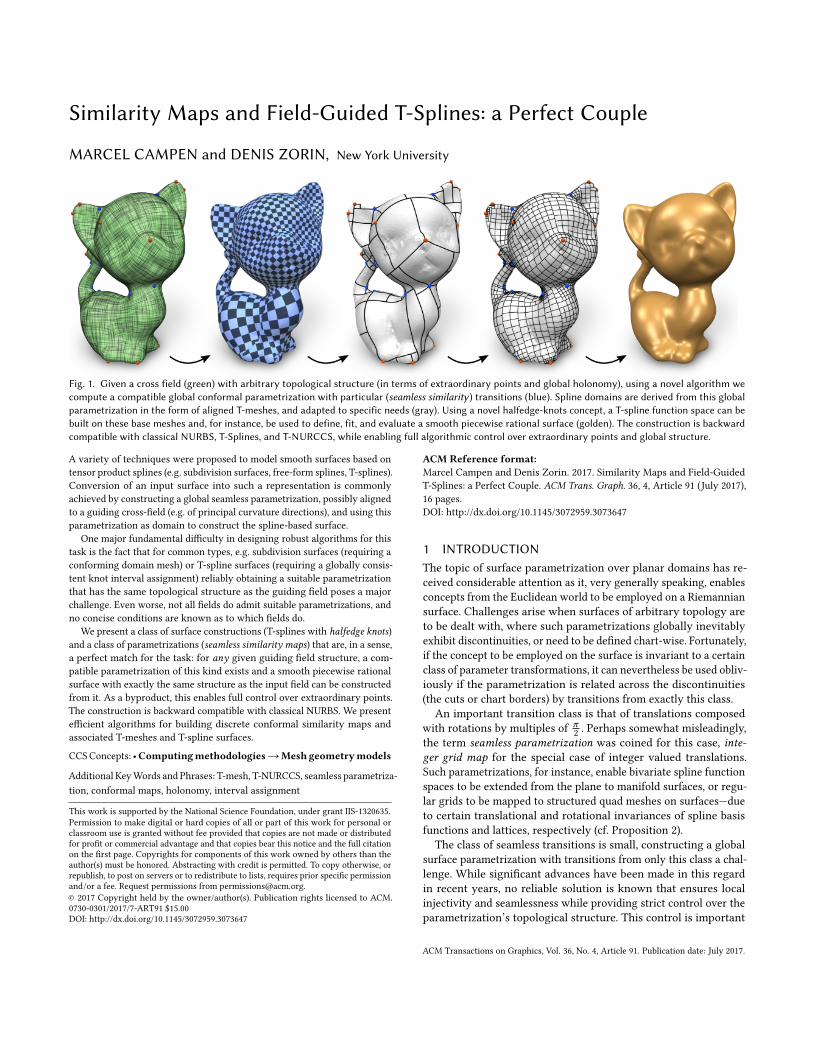
Fig. 1. Given a cross field (green) with arbitrary topological structure (in terms of extraordinary points and global holonomy), using a novel algorithm wecompute a compatible global conformal parametrization with particular (seamless similarity) transitions (blue). Spline domains are derived from this globalparametrization in the form of aligned T-meshes, and adapted to specific needs (gray). Using a novel halfedge-knots concept, a T-spline function space can bebuilt on these base meshes and, for instance, be used to define, fit, and evaluate a smooth piecewise rational surface (golden). The construction is backwardcompatible with classical NURBS, T-Splines, and T-NURCCS, while enabling full algorithmic control over extraordinary points and global structure.
A variety of techniques were proposed to model smooth surfaces based on
tensor product splines (e.g. subdivision surfaces, free-form splines, T-splines).
Conversion of an input surface into such a representation is commonly
achieved by constructing a global seamless parametrization, possibly aligned
to a guiding cross-�eld (e.g. of principal curvature directions), and using this
parametrization as domain to construct the spline-based surface.
One major fundamental di�culty in designing robust algorithms for this
task is the fact that for common types, e.g. subdivision surfaces (requiring a
conforming domain mesh) or T-spline surfaces (requiring a globally consis-
tent knot interval assignment) reliably obtaining a suitable parametrization
that has the same topological structure as the guiding �eld poses a major
challenge. Even worse, not all �elds do admit suitable parametrizations, and
no concise conditions are known as to which �elds do.
We present a class of surface constructions (T-splines with halfedge knots)and a class of parametrizations (seamless similarity maps) that are, in a sense,
a perfect match for the task: for any given guiding �eld structure, a com-
patible parametrization of this kind exists and a smooth piecewise rational
surface with exactly the same structure as the input �eld can be constructed
from it. As a byproduct, this enables full control over extraordinary points.
The construction is backward compatible with classical NURBS. We present
e�cient algorithms for building discrete conformal similarity maps and
associated T-meshes and T-spline surfaces.
CCS Concepts: •Computingmethodologies→Mesh geometrymodels
Additional Key Words and Phrases: T-mesh, T-NURCCS, seamless parametriza-
tion, conformal maps, holonomy, interval assignment
This work is supported by the National Science Foundation, under grant IIS-1320635.
Permission to make digital or hard copies of all or part of this work for personal or
classroom use is granted without fee provided that copies are not made or distributed
for pro�t or commercial advantage and that copies bear this notice and the full citation
on the �rst page. Copyrights for components of this work owned by others than the
author(s) must be honored. Abstracting with credit is permitted. To copy otherwise, or
republish, to post on servers or to redistribute to lists, requires prior speci�c permission
and/or a fee. Request permissions from [email protected].
© 2017 Copyright held by the owner/author(s). Publication rights licensed to ACM.
0730-0301/2017/7-ART91 $15.00
DOI: http://dx.doi.org/10.1145/3072959.3073647
ACM Reference format:Marcel Campen and Denis Zorin. 2017. Similarity Maps and Field-Guided
T-Splines: a Perfect Couple. ACM Trans. Graph. 36, 4, Article 91 (July 2017),
16 pages.
DOI: http://dx.doi.org/10.1145/3072959.3073647
1 INTRODUCTIONThe topic of surface parametrization over planar domains has re-
ceived considerable attention as it, very generally speaking, enables
concepts from the Euclidean world to be employed on a Riemannian
surface. Challenges arise when surfaces of arbitrary topology are
to be dealt with, where such parametrizations globally inevitably
exhibit discontinuities, or need to be de�ned chart-wise. Fortunately,
if the concept to be employed on the surface is invariant to a certain
class of parameter transformations, it can nevertheless be used obliv-
iously if the parametrization is related across the discontinuities
(the cuts or chart borders) by transitions from exactly this class.
An important transition class is that of translations composed
with rotations by multiples ofπ2
. Perhaps somewhat misleadingly,
the term seamless parametrization was coined for this case, inte-ger grid map for the special case of integer valued translations.
Such parametrizations, for instance, enable bivariate spline function
spaces to be extended from the plane to manifold surfaces, or regu-
lar grids to be mapped to structured quad meshes on surfaces—due
to certain translational and rotational invariances of spline basis
functions and lattices, respectively (cf. Proposition 2).
The class of seamless transitions is small, constructing a global
surface parametrization with transitions from only this class a chal-
lenge. While signi�cant advances have been made in this regard
in recent years, no reliable solution is known that ensures local
injectivity and seamlessness while providing strict control over the
parametrization’s topological structure. This control is important
ACM Transactions on Graphics, Vol. 36, No. 4, Article 91. Publication date: July 2017.
91:2 • Marcel Campen and Denis Zorin
as it concerns such signi�cant features as the parametrization’s sin-
gularities (which, e.g., imply extraordinary points in spline surfaces
or irregular vertices in quad meshes) as well as its global holonomy
(cf. Section 2). The latter is of particular relevance when the global
directional �ow of the parametrization’s isolines is sought to be
in�uenced, e.g. using a guiding cross �eld (cf. Figure 1 left). Further-
more, even when a reliable, practical solution becomes available, it
is known that not every cross �eld can be matched topologically by
a seamless parametrization. This is discussed in detail in Section 2.
ContributionWe introduce two new concepts which, in tandem, provide a remedy.
• Seamless similarity maps. This class of parametrizations has
transitions that are compositions of translations, rotations by
multiples ofπ2
, and (positive, isotropic) scalings. It thus forms
a superclass of seamless maps. This class is large enough that
for any surface and any �eld topology a matching seamless
similarity map exists. This statement even holds when we focus
speci�cally on conformal seamless similarity maps (cf. Figure 3).
This allows us to leverage results for conformal mapping and to
present a practical algorithm for the construction of maps from
this class, whose e�ciency and robustness we demonstrate on
a challenging benchmark.
• T-splineswith halfedge knots. This construction is a remark-
ably simple generalization of classical T-splines: instead of as-
signing a single knot interval per edge of the control mesh, we
assign two values, one for each side of the edge (subject to local
conditions, cf. Figure 2). This removes a non-inherent restric-
tion that limited applicability to domains built from the smaller
class of seamless maps. These splines can thus be de�ned based
on seamless similarity maps instead. We demonstrate that this,
for instance, opens up possibilities for piecewise polynomial
or rational smooth surface constructions with full structural
control (over extraordinary points and global ‘edge �ow’)
Herein we speci�cally focus on extending bi-cubic T-splines and
their more generic version T-NURCCS [Sederberg et al. 2003], and
demonstrate their use in the context of surface representation. Our
surfaces are piecewise rational bi-cubic and C2away from extraor-
dinary points, andC1at extraordinary points (or G2
and G1, respec-
tively, in the terminology of geometric continuity). The approach is
more general, though, and other degrees and similar function space
constructions could be employed, as long as they support T-joints.
Our generalization does not obstruct common local control mesh
structure requirements such as well-separation of extraordinary
vertices [Li et al. 2010; Sederberg et al. 2003] or non-intersecting
T-extensions for analysis-suitable T-splines [Li et al. 2012].
Our algorithm for seamless similarity map construction extends
conformal maps to surfaces of arbitrary topology, using a special
type of cut conditions controlling global holonomy properties of
the map. We believe use cases other than T-splines can bene�t from
this, possibly with some changes, as well. Our scenario does not
require maps to be conformal; the initial map can thus be further op-
timized (within the class of seamless similarity maps), e.g. for other
distortion measures and directional alignment, using established
techniques with local injectivity constraints.
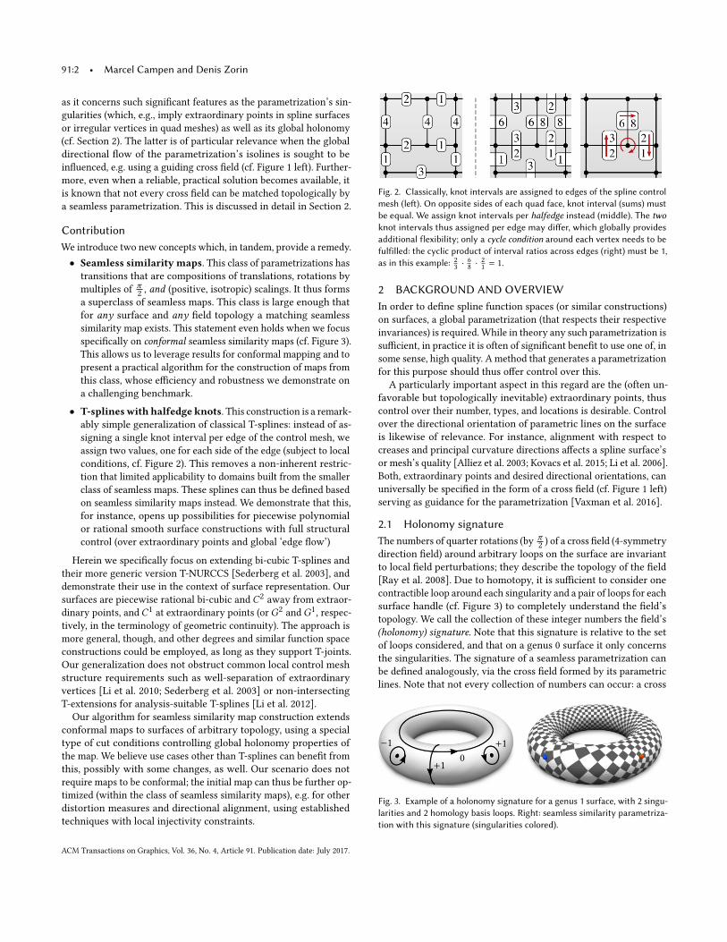
Fig. 2. Classically, knot intervals are assigned to edges of the spline controlmesh (le�). On opposite sides of each quad face, knot interval (sums) mustbe equal. We assign knot intervals per halfedge instead (middle). The twoknot intervals thus assigned per edge may di�er, which globally providesadditional flexibility; only a cycle condition around each vertex needs to befulfilled: the cyclic product of interval ratios across edges (right) must be 1,as in this example: 2
3· 68· 21= 1.
2 BACKGROUND AND OVERVIEWIn order to de�ne spline function spaces (or similar constructions)
on surfaces, a global parametrization (that respects their respective
invariances) is required. While in theory any such parametrization is
su�cient, in practice it is often of signi�cant bene�t to use one of, in
some sense, high quality. A method that generates a parametrization
for this purpose should thus o�er control over this.
A particularly important aspect in this regard are the (often un-
favorable but topologically inevitable) extraordinary points, thus
control over their number, types, and locations is desirable. Control
over the directional orientation of parametric lines on the surface
is likewise of relevance. For instance, alignment with respect to
creases and principal curvature directions a�ects a spline surface’s
or mesh’s quality [Alliez et al. 2003; Kovacs et al. 2015; Li et al. 2006].
Both, extraordinary points and desired directional orientations, can
universally be speci�ed in the form of a cross �eld (cf. Figure 1 left)
serving as guidance for the parametrization [Vaxman et al. 2016].
2.1 Holonomy signatureThe numbers of quarter rotations (by
π2
) of a cross �eld (4-symmetry
direction �eld) around arbitrary loops on the surface are invariant
to local �eld perturbations; they describe the topology of the �eld
[Ray et al. 2008]. Due to homotopy, it is su�cient to consider one
contractible loop around each singularity and a pair of loops for each
surface handle (cf. Figure 3) to completely understand the �eld’s
topology. We call the collection of these integer numbers the �eld’s
(holonomy) signature. Note that this signature is relative to the set
of loops considered, and that on a genus 0 surface it only concerns
the singularities. The signature of a seamless parametrization can
be de�ned analogously, via the cross �eld formed by its parametric
lines. Note that not every collection of numbers can occur: a cross
−1 +1
0
+1
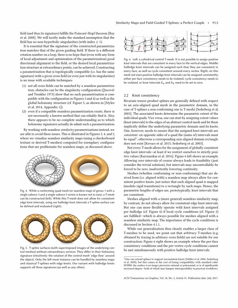
Fig. 3. Example of a holonomy signature for a genus 1 surface, with 2 singu-larities and 2 homology basis loops. Right: seamless similarity parametriza-tion with this signature (singularities colored).
ACM Transactions on Graphics, Vol. 36, No. 4, Article 91. Publication date: July 2017.
Similarity Maps and Field-Guided T-Splines: a Perfect Couple • 91:3
�eld (and thus its signature) ful�lls the Poincaré-Hopf theorem [Ray
et al. 2008]. We will tacitly make the standard assumption that the
�eld has no non-hyperbolic singularities (with index ≥ 1).
It is essential that the signature of the constructed parametriza-
tion matches that of the given guiding �eld. If there is a di�erent
rotation number on a loop, there is no hope that (even with any form
of local adjustment and optimization of the parametrization) good
directional alignment to the �eld, or the desired local parametriza-
tion structure at extraordinary points, can be achieved. Constructing
a parametrization that is topologically compatible (i.e. has the same
signature) with a given cross �eld (or even just with its singularities)
is an issue with available techniques:
(1) not all cross �elds can be matched by a seamless parametriza-
tion; obstacles can be the singularity con�guration ([Jucovič
and Trenkler 1973] show that no such parametrization is com-
patible with the con�guration in Figures 3 and 4) as well as the
global holonomy structure (cf. Figure 5, as shown in [Myles
et al. 2014, Appendix 1]).
(2) even if a compatible seamless parametrization exists, there is
not necessarily a known method that can reliably �nd it. Also,
there appears to be no complete understanding as to which
holonomy signatures actually do admit such a parametrization.
By working with seamless similarity parametrizations instead, we
are able to avoid these issues. This is illustrated in Figures 3, 4, and 5,
where we visualize seamless similarity maps (using a checkerboard
texture or derived T-meshes) computed for exemplary con�gura-
tions that are problematic for seamless maps, as discussed above.
Fig. 4. While a conforming quad mesh (or seamless map) of genus 1 with asingle valence 3 and a single valence 5 vertex is known not to exist, a T-meshcan be constructed (le�). While this T-mesh does not allow for consistentedge knot intervals, using our halfedge knot intervals a T-spline surface canbe defined and evaluated (right).
Fig. 5. T-spline surfaces (with superimposed images of the underlying con-trol meshes) without extraordinary vertices. They di�er in their holonomysignature (intuitively: the rotation of the control mesh ‘edge flow’ aroundthe object). Only the le�-most instance can be handled by seamless mapsand classical T-splines with edge knots. Our variant with halfedge knotssupports all three signatures (as well as any other).
ka kb
Fig. 6. Le�: a cylindrical control T-mesh. It is not possible to assign positiveknot intervals that are consistent in every face to the vertical edges. Middle:halfedge knot intervals can be assigned such that they are consistent inevery face, as well as cycle consistent around every vertex. Right: on thismesh not even positive halfedge knot intervals can be assigned consistently;either per-face consistency needs to be violated, cycle consistency needs tobe violated, or knot intervals ka and kb need to be set to zero.
2.2 Knot consistencyBivariate tensor-product splines are generally de�ned with respect
to an axis-aligned quad mesh in the parametric domain, in the
case of T-splines a non-conforming one (a T-mesh) [Sederberg et al.
2003]. The associated knots determine the parametric extent of the
individual quads. Vice versa, one can start by assigning extent values
(knot intervals) to the edges of an abstract control mesh and let them
implicitly de�ne the underlying parametric domain and its knots.
One, however, needs to ensure that the assigned knot intervals are
consistent: on opposite sides of a quad the (sums of) intervals must
be equal1; otherwise a corresponding axis-aligned domain rectangle
does not exist [Kovacs et al. 2015; Sederberg et al. 2003].
Not every T-mesh allows for the assignment of globally consistent
edge knot intervals—at least if we restrict ourselves to strictly posi-
tive values [Karciauskas et al. 2016]. Figure 6 left shows an example.
Allowing zero intervals of course always leads to feasibility (just
consider the trivial solution), but intervals may uncontrollably be
forced to be zero, inadvertently lowering continuity.
Meshes (whether conforming or non-conforming) that are de-
rived from (i.e. aligned with) a seamless map always allow for con-
sistent positive knots: just notice that each aligned quad is mapped
(modulo rigid transitions) to a rectangle by such maps. Hence, the
parametric lengths of edges are, prototypically, knot intervals that
are consistent.
Meshes aligned with a (more general) seamless similarity map,
by contrast, do not always allow for consistent edge knot intervals.
But one can more �exibly operate with knot intervals assigned
per halfedge (cf. Figure 6) if local cycle conditions (cf. Figure 2)
are ful�lled—which is always possible for meshes aligned with a
seamless similarity map. The importance of the cycle conditions is
discussed in Section 4.1.1.
While our generalization thus clearly enables a larger class of
T-meshes to be used, we point out that arbitrary T-meshes (e.g.
obtained by tracing in arbitrary cross �elds) are not suitable for our
construction: Figure 6 right shows an example where the per-face
consistency conditions and the per-vertex cycle conditions cannot
be met simultaneously with positive halfedge knot intervals.
1One can extend splines to support inconsistent knots [Müller et al. 2006; Sederberg
et al. 2008], but this comes at the cost of losing compatibility with standard cubic
NURBS; the surface is no longer piecewise rational or polynomial, or is of signi�cantly
increased degree—both of which may hamper interoperability in practical work�ows.
ACM Transactions on Graphics, Vol. 36, No. 4, Article 91. Publication date: July 2017.
91:4 • Marcel Campen and Denis Zorin
OverviewWe begin by showing the following results:
• Piecewise rational bi-cubic spline surfaces can be de�ned based
on T-meshes with consistent halfedge knots (Section 4),
• T-meshes aligned with seamless similarity maps allow for such
consistent halfedge knots (Section 5),
• Such a seamless similarity map exists for any cross �eld’s holo-
nomy signature (Section 6).
We then exploit these results algorithmically, following these steps
in our construction, as illustrated in Figure 1:
(1) Compute a seamless similarity parametrization using a con-
strained conformal map, matching the desired holonomy sig-
nature. An optimization of this initial map for directional align-
ment and other objectives can follow (Section 7).
(2) Construct a suitable aligned control T-mesh, containing the
set of desired spline control vertices, out of isoline segments
of this parametrization and assign consistent halfedge knot
intervals (Section 8).
(3) Evaluate the T-spline using basis function domains, and tran-
sition functions between these domains, that are derived from
the consistent knot intervals (Section 4.2).
3 RELATED WORKSeamless Parametrization. For global parametrizations to be of use
in the context of generating parametric domains for classical tensor-
product spline surfaces, they need to be seamless, as discussed in the
previous sections. A variety of methods have been described for the
generation of such parametrizations [Aigerman and Lipman 2015;
Bommes et al. 2009; Campen et al. 2015; Ebke et al. 2016; Kälberer
et al. 2007; Myles et al. 2014; Myles and Zorin 2012, 2013; Tong et al.
2006], often in the context of quad mesh generation or seamless
texturing [Ray et al. 2010].
Conformal Parametrization. For the construction of seamless sim-
ilarity parametrizations, we make use of conformal maps. There is
a variety of approaches to conformal map construction, based on
circle patterns [Bowers and Hurdal 2003; Kharevych et al. 2006],
discrete Ricci �ow [Chow and Luo 2003; Jin et al. 2007], or variations
thereof [Springborn et al. 2008]. Conformal maps have been used
in the concrete context of T-spline construction before [Gu et al.
2008; He et al. 2006]. These latter approaches are based on a speci�c
mapping technique [Gu and Yau 2003] that supports extraordinary
vertices of valence 8, 12, 16, . . . only.
Just like the above seamless metric parametrization techniques,
these conformal techniques cannot typically guarantee �nding a
valid map in general. Most importantly, there can be obstructions
to the existence of any proper map in the discrete setting, caused
by un�t tessellation. Few works have addressed this problem, e.g.
[Luo 2004], who shows that dynamic edge �ips can theoretically be
employed in the course of conformal �ow.
We have not seen the global map behavior (in terms of holonomy
or rotation around non-contractible loops) being addressed and
controlled in these works (as opposed to some works on seamless
parametrization, e.g. [Campen and Kobbelt 2014]). This control is
an essential requirement and core aspect of our method.
It is well known that any surface admits some conformal atlas
[Postnikov 2001, Ch. 14]. We show that this even holds for very spe-
ci�c conformal atlases, with seamless similarity transitions between
charts. These build the foundation of our spline construction.
Smooth Surfaces. Smooth surface representations based on poly-
nomial patches, NURBS, and, more generally, subdivision, were
traditionally based on control meshes which are conforming, most
prominently conforming quad meshes [Cashman 2012; Farin 2002],
which are closely related to seamless parametrizations. Some works
have addressed the problem of automatically constructing such
meshes for given shapes, e.g. [Boier-Martin et al. 2004; Eck and
Hoppe 1996; Panozzo et al. 2011]. Hierarchical control meshes later
provided more freedom (in terms of local resolution adaptation ca-
pabilities) in this context [Bertram et al. 2004; Khodakovsky et al.
2000; Lounsbery et al. 1997; Zorin et al. 1997].
Even more �exibility was gained through constructions based
on non-conforming quad meshes, so-called T-meshes. Examples
are T-splines [Sederberg et al. 2004], T-NURCCS [Sederberg et al.
2003], PHT-splines [Deng et al. 2008], GPT-splines [Li et al. 2010],
or dyadic T-subdivision [Kovacs et al. 2015]. Advantages due to this
more �exible structure, e.g. for isogeometric analysis, have been
demonstrated [Bazilevs et al. 2010].
Automatic T-Mesh Construction. The construction of arbitrary T-
meshes can be facilitated quite easily, for instance by tracing integral
curves of cross �elds [Myles et al. 2014], by growing patches [Carr
et al. 2006], or from isolines of periodic functions [Ray et al. 2006].
These T-meshes, however, are most often not suitable for spline
applications, because they do not allow for globally consistent knot
intervals (neither edge nor halfedge based).
T-meshes that allow for consistent edge-based knot intervals
have been obtained as a submesh of a conforming mesh [Eppstein
et al. 2008; Li et al. 2006; Myles et al. 2010; Sederberg et al. 2004],
as a subset of the isocurves of a seamless surface parameterization
[Campen et al. 2015; He et al. 2006], or by restricted local re�nement
as a supermesh of a conforming mesh [Sederberg et al. 2003; Wang
et al. 2012]. However, robustly constructing a conforming quad
mesh or a seamless surface map with the desired topology to start
with is a major issue, as discussed in Section 2.1.
4 SPLINE SURFACES WITH HALFEDGE KNOTSIn this section, we de�ne our version of T-spline surfaces with
halfedge knot intervals in detail. To simplify exposition, we focus
on surfaces without boundary and we do not consider zero inter-
vals here (which can be of interest to selectively lower the local
continuity order, e.g. for creasing).
T-meshes. A T-mesh is a mesh with quad faces; two quad faces of
a T-mesh may intersect over a part of a common edge (as opposed
to a conforming mesh, where faces only intersect over entire edges
or vertices). A vertex is a T-joint with respect to an adjacent quad if
it is contained in the interior of an edge of this quad. We de�ne the
extended valence of a vertex as the number of incident edges, plus
the number of quads for which the vertex is a T-joint. We say that a
vertex is extraordinary if its extended valence is di�erent from four.
All other vertices are called regular.
ACM Transactions on Graphics, Vol. 36, No. 4, Article 91. Publication date: July 2017.
Similarity Maps and Field-Guided T-Splines: a Perfect Couple • 91:5
Halfedge knots. To de�ne a T-spline we need to specify knot
interval values. Here our construction di�ers from the classical one
in a crucial way, as we do not assign a unique knot interval for
an edge. Instead, we assign a knot interval per halfedge h, i.e., a
(face, edge) pair. For a halfedge h of edge e , let h′ denote the other
(opposite) halfedge of e .
For each halfedge h of the T-mesh, corresponding to edge e and facef , we assign a knot interval value k(h) = k(e, f ) ∈ R>0. These knotintervals need to satisfy two requirements:• the sum of the knot intervals of halfedges on a side of a quad is
equal to the sum on the opposite side (consistency condition),• the ratios sh = k(h)/k(h′) of intervals of opposite halfedges satisfy∏
h∈Hv sh = 1 at every vertex v (cycle condition).
Above, the set Hv contains one halfedge of each edge incident
to v , chosen consistently (e.g. the ones associated with the faces
that lie clockwise of the respective edges around v). Notice that this
de�nition reduces to classical de�nitions of tensor-product spline
and T-spline control meshes, which carry knot intervals per edge, if
we require sh = 1 for each halfedge h.
Admissibility. We call an assignment of halfedge knot intervals
satisfying the above conditions admissible. A T-mesh is called admis-
sible if an admissible assignment of positive knot intervals exists.
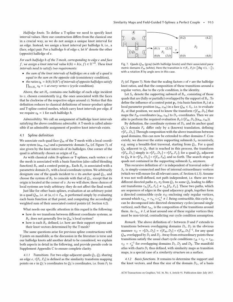
4.1 Spline definitionWe associate each quad face Qm of the T-mesh with a local coordi-
nate system (um ,vm ) and a parametric domain Fm (cf. Figure 7), of
size given by the knot intervals of its halfedges. One corner of the
quad is arbitrarily chosen as origin of Fm .
As with classical cubic B-splines or T-splines, each vertex v of
the mesh is associated with a basis function (also called blending
function) Bv and a control point pv . Each Bv is associated with a
parametric domainDv with a local coordinate system. We arbitrarily
designate one of the quads incident to v its anchor quad Qv , and
choose the system of Bv to coincide with that of Qv , except that its
origin is located at the corner ofv . As we will show, these choices of
local systems are truly arbitrary; they do not a�ect the �nal result.
Just like for other basis splines, evaluation at an arbitrary point
in a quad Qm , i.e. at (u,v) ∈ Fm , is performed simply by evaluating
each basis function at that point, and computing the accordingly
weighted sum of their associated control points (cf. Section 4.2).
What needs our speci�c attention in this regard is the following:
• how do we transform between di�erent coordinate systems, as
Bv does not generally live in Qm ’s local system?
• how is each Bv de�ned, i.e. how are their support regions and
their knot vectors determined by the T-mesh?
The same questions arise for previous spline constructions with
T-joints on manifolds; as the discussion in the literature is terse and
our halfedge knots add another detail to be considered, we explain
both aspects in detail in the following, and provide pseudo code in
Supplement Appendix C to ensure complete clarity.
4.1.1 Transitions. For two edge-adjacent quads Q1,Q2 sharing
an edge e , τ [F1, F2] is de�ned as the similarity transform mapping
points on e in Q1’s coordinates to Q2’s coordinates, i.e. from F1 to
τF1
F2
Q1
Q2
Fig. 7. �ads Qm (gray) (with halfedge knots) and their associated para-metric domains Fm (white). Here the transition is τ (F1, F2)= 3
2Rq +(1, − 3
2),
with a rotation R by angle zero in this case.
F2 (cf. Figure 7). Note that the scaling factors s of τ are the halfedge
knot ratios, and that the composition of these transitions around a
regular vertex, due to the cycle condition, is the identity.
Let Sv denote the supporting submesh of Bv , consisting of those
quads that are (fully or partially) overlapped by the support of Bv . To
de�ne the in�uence of a control point pv (via basis function Bv ) at a
local parameter position (um ,vm ) in a faceQm ∈ Sv , i.e. to evaluate
Bv at that position, we need to know the transform τ [Fm ,Dv ] that
maps the Fm -coordinates (um ,vm ) to Dv -coordinates. Then we are
able to perform the required evaluation Bv (τ [Fm ,Dv ](um ,vm )).By de�nition, the coordinate systems of Dv and its anchor quad
Qv ’s domain Fv di�er only by a (known) translation, de�ning
τ [Fv ,Dv ]. Through composition with the above transitions between
quad domains, this can now be extended to other domains F . Con-
cretely, we discover the entire supporting submesh Sv recursively,
e.g. using a breadth-�rst traversal, starting from Qv . For a quad
Qn adjacent to Qv that is reached in this process, the transform
τ [Fn ,Dv ] simply is τ [Fv ,Dv ] ◦ τ [Fn , Fv ]; for a quad Qo adjacent
to Qn it is τ [Fn ,Dv ] ◦ τ [Fo , Fn ], and so forth. The search stops at
quads not contained in the supporting submesh Sv anymore.
This recursive de�nition of τ is independent of traversal order—if
Sv is simply-connected and free of internal extraordinary vertices
(which we will ensure for all relevant cases, cf. Section 4.1.3). Assume
it was not well-de�ned, not path independent, i.e. there are two
di�erent directed paths π1,π2 from Qv to some Qo leading to di�er-
ent transforms τπ1 [Fo , Fv ] , τπ2 [Fo , Fv ]. These two paths, which
are sequences of edges in the quad adjacency graph, together form
a directed contractible cycle π12 enclosing only regular vertices,
around which τπ12 = τπ2 ◦τ−1π1 , I . Being contractible, this cycle π12
can be decomposed into directed elementary cycles (around single
vertices), such that τπ12 is the composition of the transitions around
them. As τπ12 , I , at least around one of these regular vertices they
must be non-trivial, contradicting our cycle condition assumption.
Remark. The above de�nition of τ between D and F extends to
transitions between overlapping domains Di , D j in the obvious
manner: τi j = τ [Di ,D j ] = τ [Fm ,D j ] ◦ τ [Fm ,Di ]−1
, for any quad
Qm overlapped byDi andD j . Away from extraordinary points these
transitions satisfy the usual chart cycle conditions τjk ◦ τi j = τik ,
τi j = τ−1ji for overlapping domains Di , D j and Dk . The manifold
atlas with charts Di thus de�ned, with similarity maps as transition
maps, is a special case of a similarity structure on a surface.
4.1.2 Basis functions. It remains to determine the support and
the knot vectors, and thus the size of the domain Dv , of a basis
ACM Transactions on Graphics, Vol. 36, No. 4, Article 91. Publication date: July 2017.
91:6 • Marcel Campen and Denis Zorin
function Bv . Note that these knots are relative to the local coordinate
system chosen for Bv .
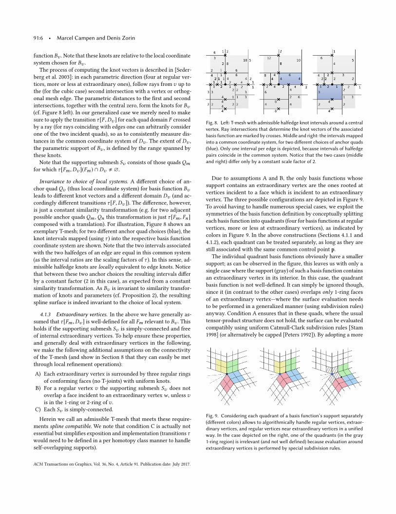
The process of computing the knot vectors is described in [Seder-
berg et al. 2003]: in each parametric direction (four at regular ver-
tices, more or less at extraordinary ones), follow rays from v up to
the (for the cubic case) second intersection with a vertex or orthog-
onal mesh edge. The parametric distances to the �rst and second
intersections, together with the central zero, form the knots for Bv(cf. Figure 8 left). In our generalized case we merely need to make
sure to apply the transition τ [F ,Dv ] for each quad domain F crossed
by a ray (for rays coinciding with edges one can arbitrarily consider
one of the two incident quads), so as to consistently measure dis-
tances in the common coordinate system of Dv . The extent of Dv ,
the parametric support of Bv , is de�ned by the range spanned by
these knots.
Note that the supporting submesh Sv consists of those quads Qmfor which τ [Fm ,Dv ](Fm ) ∩ Dv , ∅.
Invariance to choice of local systems. A di�erent choice of an-
chor quad Qv (thus local coordinate system) for basis function Bvleads to di�erent knot vectors and a di�erent domain Dv (and ac-
cordingly di�erent transitions τ [F ,Dv ]). The di�erence, however,
is just a constant similarity transformation (e.g. for two adjacent
possible anchor quads Qm , Qn this transformation is just τ [Fm , Fn ]composed with a translation). For illustration, Figure 8 shows an
exemplary T-mesh; for two di�erent anchor quad choices (blue), the
knot intervals mapped (using τ ) into the respective basis function
coordinate system are shown. Note that the two intervals associated
with the two halfedges of an edge are equal in this common system
(as the interval ratios are the scaling factors of τ ). In this sense, ad-
missible halfedge knots are locally equivalent to edge knots. Notice
that between these two anchor choices the resulting intervals di�er
by a constant factor (2 in this case), as expected from a constant
similarity transformation. As Bv is invariant to similarity transfor-
mation of knots and parameters (cf. Proposition 2), the resulting
spline surface is indeed invariant to the choice of local system.
4.1.3 Extraordinary vertices. In the above we have generally as-
sumed that τ [Fm ,Dv ] is well-de�ned for all Fm relevant to Bv . This
holds if the supporting submesh Sv is simply-connected and free
of internal extraordinary vertices. To help ensure these properties,
and generally deal with extraordinary vertices in the following,
we make the following additional assumptions on the connectivity
of the T-mesh (and show in Section 8 that they can easily be met
through local re�nement operations):
A) Each extraordinary vertex is surrounded by three regular rings
of conforming faces (no T-joints) with uniform knots.
B) For a regular vertex v the supporting submesh Sv does not
overlap a face incident to an extraordinary vertex w , unless vis in the 1-ring or 2-ring of v .
C) Each Sv is simply-connected.
Herein we call an admissible T-mesh that meets these require-
ments spline compatible. We note that condition C is actually not
essential but simpli�es exposition and implementation (transitions τwould need to be de�ned in a per homotopy class manner to handle
self-overlapping supports).
Fig. 8. Le�: T-mesh with admissible halfedge knot intervals around a centralvertex. Ray intersections that determine the knot vectors of the associatedbasis function are marked by crosses. Middle and right: the intervals mappedinto a common coordinate system, for two di�erent choices of anchor quads(blue). Only one interval per edge is depicted, because intervals of halfedgepairs coincide in the common system. Notice that the two cases (middleand right) di�er only by a constant scale factor of 2.
Due to assumptions A and B, the only basis functions whose
support contains an extraordinary vertex are the ones rooted at
vertices incident to a face which is incident to an extraordinary
vertex. The three possible con�gurations are depicted in Figure 9.
To avoid having to handle numerous special cases, we exploit the
symmetries of the basis function de�nition by conceptually splitting
each basis function into quadrants (four for basis functions at regular
vertices, more or less at extraordinary vertices), as indicated by
colors in Figure 9. In the above constructions (Sections 4.1.1 and
4.1.2), each quadrant can be treated separately, as long as they are
still associated with the same common control point p.
The individual quadrant basis functions obviously have a smaller
support; as can be observed in the �gure, this leaves us with only a
single case where the support (gray) of such a basis function contains
an extraordinary vertex in its interior. In this case, the quadrant
basis function is not well-de�ned. It can simply be ignored though,
since it (in contrast to the other cases) overlaps only 1-ring faces
of an extraordinary vertex—where the surface evaluation needs
to be performed in a generalized manner (using subdivision rules)
anyway. Condition A ensures that in these quads, where the usual
tensor-product structure does not hold, the surface can be evaluated
compatibly using uniform Catmull-Clark subdivision rules [Stam
1998] (or alternatively be capped [Peters 1992]). By adopting a more
Fig. 9. Considering each quadrant of a basis function’s support separately(di�erent colors) allows to algorithmically handle regular vertices, extraor-dinary vertices, and regular vertices near extraordinary vertices in a unifiedway. In the case depicted on the right, one of the quadrants (in the gray1-ring region) is irrelevant (and not well defined) because evaluation aroundextraordinary vertices is performed by special subdivision rules.
ACM Transactions on Graphics, Vol. 36, No. 4, Article 91. Publication date: July 2017.
Similarity Maps and Field-Guided T-Splines: a Perfect Couple • 91:7
complex, non-uniform scheme, e.g. [Cashman 2012; Kovacs et al.
2015; Li et al. 2016; Sederberg et al. 2003], one could reduce the
required number of regular rings to two.
4.2 Spline evaluationTo de�ne precisely the evaluation of the surface at an arbitrary point
in a quadQm (not incident to an extraordinary vertex), i.e. at (u,v) ∈Fm , let Cm be the set of all overlapping quadrant basis functions Bi(for which Qm ∈ Si ); let pi be the control point associated with Bi .Then we de�ne the surface evaluation as
F (u,v) =
∑Bi ∈Cm pi Bi (τ [Fm ,Di ](u,v))∑Bi ∈Cm Bi (τ [Fm ,Di ](u,v))
(1)
For a quad incident to an extraordinary vertex, we rely on Catmull-
Clark subdivision instead, to evaluate a C1surface [Stam 1998].
Proposition 1. The surface F de�ned by (1)
• is invariant with respect to arbitrary seamless similarity trans-forms applied to domains Di and their knot vectors, thus in par-ticular to the choice of local coordinate systems,
• is a piecewise rational C2 (or “G2”) surface away from extraordi-nary points.
A proof can be found in Appendix A; it is based on the following
observation of parametric similarity invariance of basis functions:
Proposition 2. Let the 2D tensor-product B-spline basis functionB[u, v](u,v) = B[u](u)B[v](v) be de�ned by knots u1, . . . ,uk andv1, . . . ,vk ; u, v are vectors of knots for two coordinate directions. Let(u ′,v ′) = τ (u,v) = sR[u,v]T + t be a similarity transformation ofthe parametric domain B, where R is a rotation by kπ/2, k ∈ Z, s > 0
is a scale factor, and t a translation vector. De�ne u′ and v′ as vectorsof knots u ′i and v
′i obtained as coordinates of τ (ui ,vi ). Then
B[u′, v′](u ′,v ′) = B[u, v](u,v) (2)
A proof can be found in Appendix A as well.
5 SPLINE-COMPATIBLE T-MESHES FROM SIMILARITYMAPS
To simplify the seemingly complex problem of constructing an ad-
missible (or ultimately spline-compatible) T-mesh for a surfaceM
(the conditions on knot intervals are nonlinear), we �rst reduce it
to the problem of �nding a seamless similarity map. The construc-
tion of such a map is then addressed in the following Sections 6
(theoretical background) and 7 (computational algorithm).
Consider a surface M with an embedded set of curves that cut it
to a disk (cut graph). Denote the resulting cut surface with boundary
Mc . A continuous, locally injective map f (p) : Mc → R2 is a
seamless similarity map if for each two coinciding points q, q′ on
di�erent sides of the cut the parametric coordinates are related by a
seamless similarity transformation, i.e. f (q′) = σ (f (q)) = sR f (q)+t,where R is a rotation by kπ/2, k ∈ Z, and these transitions σ ful�ll
the above mentioned cycle condition around any regular point. Note
that this in particular implies that s , R, and t are constant along each
branch of the cut graph (away from extraordinary points).
The proof of the following proposition is constructive, and de�nes
a way to generate T-meshes and assign admissible halfedge knot
intervals from a seamless similarity parametrization.
Proposition 3. For a seamless similarity parametrization f onMc , any T-mesh embedded in M whose edges follow f ’s parametriclines and whose vertices include f ’s singularities is admissible, andsuch a T-mesh always exists.
Proof. An algorithm demonstrating existence is given in [Myles
et al. 2014]: by tracing a general cross-�eld on a surface (in our
special case: the �eld de�ned by the parametric lines of f ) starting
from extraordinary points, one can obtain an embedded T-mesh
with the required properties, using a modi�ed motorcycle graph
algorithm [Eppstein et al. 2008]. As in our case parametric lines
rather than general cross-�elds need to be traced [Campen et al.
2015], in practice tracing is particularly simple compared to the
general setting of [Myles et al. 2014; Ray and Sokolov 2014].
For the �rst part of the proposition, assume the cut coincides with
edges of an embedded T-mesh, i.e. the cut nowhere runs through
faces. We assign as knot interval value to each halfedge its length
in parameter space, under f . As each face has a rectangular image
(due to f -aligned edges), these knot intervals are consistent per face.
Furthermore, the knot ratio at each edge equals the scale factor of
the similarity transition σ on the cut coinciding with the edge (or is
1 if there is no cut). Hence, as f is cycle consistent, so are the knot
intervals, proving admissibility of the T-mesh.
If the cut does not coincide with T-mesh edges, it can be deformed
to do so; then the above argument applies. This is possible in general
because the embedded T-mesh forms a cell decomposition of M (due
to all faces having disk topology), thus is homotopic to M . �
In practice, such a cut deformation does not need to be performed
explicitly. When computing parametric lengths of halfedges in a face,
one simply maps all parameter values into a common local system
(e.g. rooted at a corner of the face) by applying all cut transitions
σ encountered on a path (within the face) to that corner. Cycle
consistency of the map together with simple topology of the face
ensure that the result is unique, path-independent.
6 SIMILARITY MAPS VIA CONFORMAL MAPSIn this section we establish existence of seamless similarity maps
with arbitrary signature, using conformal maps. To this end, let us
�rst make precise the notion of a cross �eld and its signature. For
a background on the (discrete) exterior calculus notation we make
use of, we refer to [Abraham et al. 1988; Desbrun et al. 2008].
Cross �eld. An assignment of quadruples (e, e⊥,−e,−e⊥) of unit-
length vectors, separated by right angles, to all points on a surface,
possibly excluding a number of isolated extraordinary points (sin-
gularities), is called a cross �eld. It has an associated di�erential
quantity, the connection 1-form ω (from which it can be recovered
up to a constant global rotation). For the discrete case this view-
point was considered in [Crane et al. 2010]. The form ω is de�ned
by 〈ω, v〉 = e⊥ · ∇ve, where ∇v is the surface derivative of e in
the direction v. This form ω, evaluated on some tangent vector v,
produces the rate of rotation of the cross �eld in direction v. The
total rotation rγ along a curve γ (with tangent t) is thus given by
rγ =
∫γ〈ω, t〉 ds (3)
ACM Transactions on Graphics, Vol. 36, No. 4, Article 91. Publication date: July 2017.
91:8 • Marcel Campen and Denis Zorin
The connection 1-form ω of a cross �eld is trivial [Crane et al.
2010], in the sense that this total rotation rγ plus the total geodesic
curvatureκtot [γ ] of the curve itself is a multiple of π/2 for any closedcurve (i.e. loop) γ . Note that the values kγ = (rγ + κ
tot [γ ])/ π2
are
the integral quarter rotation numbers that make up the signature
introduced in Section 2.1. For a seamless (similarity) map f , the
signature can be de�ned analogously, via the cross-�eld (and its
di�erential ωf ) de�ned by the tangents to the parametric lines.
Proposition 4. For any admissible holonomy signature for a sys-tem of homology loops γj , j = 1 . . . 2д and singularities pi , i = 1 . . .Non a surfaceM , there is a seamless similarity map with this signature;one such map is given by a conformal map f on the cut surfaceMc ,de�ned by the conformal factor eϕ onMc , constructed as dϕ = ?ωffrom the unique co-closed 1-form ωf onM satisfying
?dωf = K − KG , (4)∫γj〈ωf , t〉 ds = kγj
π
2
− κtot [γj ], (5)
for each j ∈ {1, . . . , 2д}. KG is the Gaussian curvature of M , andK = 2π
∑Ni=1 index(pi )δ (pi ), with δ a Dirac delta distribution.
Equation (4) is e�ectively the limit case of (5) for loops contracting
around every single point of M , thus, besides enforcing the desired
rotation numbers for singular points pi , also enforcing an index of
zero for any non-singular point [Bunin 2008].
We point out that this proposition in this form applies to the
smooth case only; the discrete setting is considered in Section 7.
Proof. Let ϕ ′ be a 0-form on the closed surface M that solves
the Poisson equation ∆ϕ ′ = ?d?dϕ ′ = K − KG . This equation has,
for the here relevant case of K being a sum of deltas, a unique
(up to an additive constant) solution ϕ ′ [Aubin 1998; Bunin 2008;
Troyanov 1991]. Note that ω ′ = ?dϕ ′ is co-closed and obviously
solves (4)—but not generally (5).
A closed genus д surface has a 2д-dimensional space of har-
monic 1-forms. Let {ω1, . . . ,ω2д} be a basis of this space, such
that
∫γj〈ωi , t〉 ds = δi j , i.e. the total rotation of ωi vanishes on all
loops but γi [Gu and Yau 2003; Tong et al. 2006, App. B]. Then
we have d(ω ′ + ciωi ) = dω ′ for any ci ∈ R due to harmonic-
ity of ωi , and
∫γj〈(ω ′ + ciωi ), t〉 ds =
∫γj〈ω ′, t〉 ds + ci
∫γj〈ωi , t〉 ds .
Hence, by choice of coe�cients ci , we can independently adjust
the rotation around the loops γj , without a�ecting (4), such that
ωf = ω′ +
∑2дi=1 ciωi uniquely solves (4) and (5).
As?ωf is closed, it is exact on the (simply-connected) cut surface
Mc , so it can indeed by integrated uniquely (up to constant global
scale), yielding the 0-form ϕ on Mc . Assuming the singular points
are contained in the cut, Mc is �at under the metric Ge2ϕ whose
Gaussian curvature isK [Aubin 1998; Schoen and Yau 1994], de�ning
a conformal map f . It is unique up to a rigid transformation. As
discussed in [Myles and Zorin 2013], ωf is indeed the di�erential of
f constructed in this way. Thus f respects the input signature.
It remains to show that f is a seamless similarity map. For this
we refer to Appendix A.
�
7 DISCRETE SIMILARITY MAPSWe now describe our algorithm to construct a discrete seamless
similarity map on a closed orientable triangle mesh M , respecting
a given signature. It is based on Proposition 4, although we do
not follow the constructive existence proof, but solve the equation
system (4) + (5) directly. This allows us to deal with discretization
issues (e.g. mesh connectivity changes) in a simpler, uni�ed manner.
7.1 BackgroundSolving this system (to then obtain ϕ via dϕ = ?ωf ) is similar to
other conformal mapping approaches, e.g. [Ben-Chen et al. 2008;
Springborn et al. 2008], though the focus typically is on simply
connected domains and thus (4) only. We need to employ an ap-
proach that supports taking (5) into account as well. We have chosen
to design an algorithm building on multiple ideas from previous
work, combining them in a novel way for the sake of generality,
performance, and robustness.
We combine three main ideas: (1) the idea of de�ning a discrete
�ow evolving the discrete 0-form ϕ (or, in our case, actually its dif-
ferential 1-form ξ = −?ωf ) according to deviation from the desired
curvature [Luo 2004], (2) performing triangle mesh connectivity
modi�cations as the �ow proceeds, to enable convergence to a
valid solution in the discrete setting [Gu et al. 2013; Luo 2004], and
(3) discretization of a single �ow step following a linear formulation
[Ben-Chen et al. 2008] which corresponds to choosing the descent di-
rection indicated by Newton’s method for the �ow [Springborn et al.
2008]. The resulting combination passes challenging stress tests as
detailed in Section 9, and, in cases that do not require numerous
mesh modi�cations, proves to be e�cient.
Setting. Given is M with discrete metricG , given by edge lengths,
and an admissible holonomy signature, e.g. one derived from a cross
�eld. The output is a piecewise-linear seamless similarity map fon M ′ (a possibly modi�ed or re�ned version of M). This map fis discrete conformal, but as we discuss in Section 7.4, it can be
taken as a starting point (with the correct signature, i.e. topology)
for optimization for other distortion measures, alignment, etc.
7.2 Solving for the 1-form ξ
We set up a system of linear equations discretizing (4) and (5). As
variables we use the discrete 1-form ξ , i.e. a scalar value ξi per
oriented edge i of the triangle mesh (the reversely oriented edge,
i ′, implicitly has the negated value, ξi′ = −ξi ), and de�ne ω = ?ξ .
Let the loops γj , j = 1, . . . , 2д, in the discrete case cyclic triangle
strips, be represented by the edges between successive triangles in
the strip, oriented consistently from left to right side of the strip.
Following [Crane et al. 2010; Myles and Zorin 2013] the integral in (5)
is discretized as
∫γ 〈?ξ , t〉ds =
∑i ∈γ ?ξi , and the Hodge star ? is
de�ned as?ξi =1
2(cotαi +cotαi′)ξi , where αi is the angle opposing
oriented edge i in the triangle left of i . The total geodesic curvature
κtot [γ ] is easily computed by summing up turning angles along the
path [Myles and Zorin 2013]. Thus, for each cycle γj , j = 1, . . . , 2д,
and each vertex (except one), we setup equations∑i ∈Ov
?ξi = 2π − kvπ
2
−KG [v],∑i ∈γj
?ξi = kγjπ
2
−κtot [γj ], (6)
ACM Transactions on Graphics, Vol. 36, No. 4, Article 91. Publication date: July 2017.
Similarity Maps and Field-Guided T-Splines: a Perfect Couple • 91:9
where Ov is the set of outwards oriented edges incident to ver-
tex v , KG [v] is the discrete Gaussian curvature at v , and kv is the
quarter rotation number around this vertex (which is related to the
singularity index as index(v) = 1 − kv/4).
As ξ is required to be a closed 1-form, we furthermore add closed-
ness conditions, i.e. for each face (except one) with (counterclock-
wise oriented) edges i, j,k :
ξi + ξ j + ξk = 0. (7)
The one vertex and face that are skipped are chosen arbitrarily
(closedness and correct curvature (via Gauss-Bonnet theorem) are
implied there). The resulting linear equation systemAξ = b has 2д+|V |−1+ |F |−1 equations, which, according to Euler’s formula, equals
the number of variables, |E |. The equations are linearly independent,
as a consequence of independence of loops (cf. [Ray et al. 2008]), so
the system has a unique solution ξ .
Due to closedness, ξ is integrable (exact) on a simply-connected
cut mesh Mc . Integration of ξ yields a logarithmic scale factor ϕ on
Mc , de�ned uniquely up to an additive constant. ϕ de�nes a discrete
metric G ′ [Luo 2004; Springborn et al. 2008] under which an edge
(v,w) that has length ` under G has length
`′ = e(ϕv+ϕw )/2` (8)
There are two problems with this linear method, cf. [Ben-Chen
et al. 2008; Springborn et al. 2008]: the resulting discrete metric G ′
is not exactly �at (away from singularities), due to discretization,
and the resulting edge lengths `′ may violate triangle inequalities.
We resolve these problems by the algorithm described in the follow-
ing, which employs the above linear solve iteratively, updating the
system at each step using the new metric, and applying adaptive
triangulation modi�cations, to maintain triangle inequalities. We
found the remeshing capability of our method to be critical (cf. Ta-
ble 1, column edge�ips), which is supported by the data of [Chien
et al. 2016] on the low success rate of a non-remeshing discrete
conformal parametrization approach on a benchmark data set.
7.3 Iterative AlgorithmThe algorithm evolves the discrete metric G ′, i.e. the edge lengths
of the cut mesh Mc . By ϕ(ξ ) we denote ϕ obtained by integrating ξon Mc , and method rescale updates edge lengths as in (8).
G ′ ← G
while | |b(G ′)| |∞ > ε
ξ ← A(G ′)−1b(G ′)
λ ← firstDegeneracy(Mc ,G′, ξ )
G ′ ← rescale(G ′, λϕ(ξ ))
For each triangle f degenerate under G ′: flip(f )
E�ectively, we view the evolution as piecewise-linear �ow: at
every step, we attempt to linearly evolve the metric from the current
metric G ′ to the rescaled metric with ϕ(ξ ) obtained from the linear
solve Aξ = b, stopping to modify the triangulation at intermediate
points where a degeneracy event occurs.
7.3.1 Degeneracy handling. Function firstDegeneracy(M,G ′, ξ )determines the �rst triangle degeneration event (if any) when con-
tinuously evolving the metric as rescale(G ′, λϕ(ξ )), i.e. it determines
the smallest “time” λ ∈ (0, 1] for which there is one (or more) de-
generate triangle in M . Degeneration events are determined as the
roots of an indicator function Ii j,k (λ) per edge (i, j) of each triangle
(i, j,k):Ii j,k (λ) = `jke
ξik λ/2+ `kieξ jk λ/2− `i j , (9)
where edge lengths ` are with respect to current metric G ′. It has
these properties: (1) for a triangle valid at λ, all three indicator
functions are positive; (2) for a degenerate triangle, the indicator
function of (at least) one edge vanishes; (3) for a triangle violating
the triangle inequality, one indicator function is negative; (4) the
function has at most two roots in λ, as shown in Appendix B.
We initially set λ0 = 1. Then, for an indicator function I with
I (λ0) < 0 (indicating a violation at time λ0), we �nd the root r in the
range (0, λ0) and set λ0 = r . Note that due to I (0) > 0 and property
(4) there is exactly one root in this range. This is repeated until all
I (λ0) ≥ 0, so as to determine the earliest degeneracy time λ0, which
is then returned by firstDegeneracy.
The method flip(f ) is used to cure the degenerate triangle f . Let
e be the longest edge of triangle f . Note that this edge is unique,
as there are no edges of length zero at any step. Edge e is �ipped
and its length computed intrinsically from the incident triangles, as
described in detail by [Fisher et al. 2007]. Notice that triangles can
never degenerate to a point (a situation that could not be resolved
by an edge �ip) as the factors e(ϕv+ϕw )/2 (cf. Equation (8)) applied
to edge lengths in each iteration are strictly positive for any choice
of ϕ. Figure 10 demonstrates the e�ect of this strategy.
Remark. One can perform �ips more generally to make the tri-
angulation intrinsically Delaunay [Fisher et al. 2007] after each
iteration. This can speed up the process in cases where otherwise
many degeneracy events would occur (cf. Table 1). Furthermore,
if required, in the end all edge �ips performed can be realized as
edge splits instead (by overlaying the meshes [Fisher et al. 2007]),
ensuring the output mesh is a re�nement of the input mesh.
7.3.2 Analysis and relation to other methods. Discrete Ricci or
Yamabe �ow [Luo 2004] can be viewed as a continuous gradient
descent of some convex energy E(ϕ) (in some instances called Ricci
energy or Yamabe energy), which describes the deviation from the
prescribed curvature (the right-hand side of (4)) under the metric
implied by ϕ. In practice very small step lengths need to be chosen
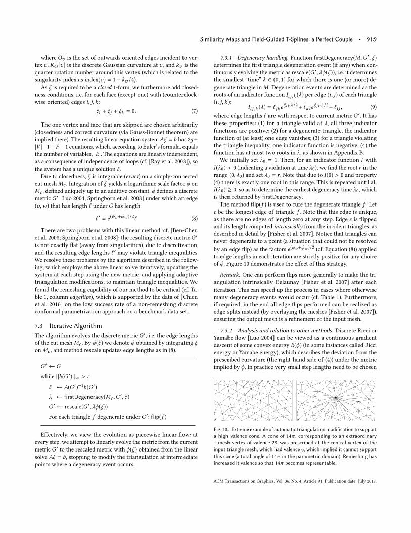
Fig. 10. Extreme example of automatic triangulation modification to supporta high valence cone. A cone of 14π , corresponding to an extraordinaryT-mesh vertex of valence 28, was prescribed at the central vertex of theinput triangle mesh, which had valence 6, which implied it cannot supportthis cone (a total angle of 14π in the parametric domain). Remeshing hasincreased it valence so that 14π becomes representable.
ACM Transactions on Graphics, Vol. 36, No. 4, Article 91. Publication date: July 2017.
91:10 • Marcel Campen and Denis Zorin
for a proper �rst order discretization of this process. Signi�cantly
faster convergence can be achieved by using a second order, Newton
method [Springborn et al. 2008]. Convergence from any starting
point (any initial curvature/metric G) is guaranteed when using a
globally convergent variant (e.g. with adaptive step size based on
trust-region or line-search techniques) [Springborn et al. 2008]. Our
algorithm can be interpreted as a variant of this approach. While
in that approach the Newton update ϕ in each step is essentially
determined via the linear system (?d?d)ϕ = µb (for an appropriately
determined step size µ), our core iteration e�ectively just uses a
di�erent bracketing (?d?)(dϕ) = µb (and exploits the additional
degrees of freedom to add terms (5) for non-contractible loops to
this underdetermined system) to determine the update for ξ (= dϕ).
An extension of the convergence analysis of [Springborn et al.
2008] to this more general setting and a proof that in the case of
convergence the resulting discrete conformal metric does indeed
yield a discrete seamless similarity map with the desired signature
can be found in [Campen and Zorin 2017]. The main open question
is whether an in�nite sequence of edge �ips could occur and hinder
convergence [Luo 2004]. The observed behavior, demonstrated in
Section 9, has not yet indicated this.
7.4 Alignment OptimizationAs T-mesh edges are aligned with isolines of the conformal map (to
guarantee admissibility), the map’s orientation (in terms of isoline
directions) directly determines T-mesh edge orientation. So far, our
focus was entirely on structure control: the map we are constructing
has exactly the signature of a guiding cross-�eld, but it may be mis-
aligned with the actual directions of the �eld. For some applications
this may not be of concern, but for others, like spline �tting, such
�eld alignment can certainly be of interest (cf. Section 2).
A very simple �rst adjustment one can make is applying a globally
constant rigid rotation to the map, such that its isolines align, as
well as rigidly possible, with the given guiding cross �eld.
To compute a further improved version of the map, we propose
to set up an optimization problem based on the quadratic cross �eld
alignment objective of [Bommes et al. 2009], with conservative con-
vex local injectivity constraints (as described by [Lipman 2012] or
[Bommes et al. 2013]), and linear constraints that �x the transitions
across cuts, thereby preserving seamless similarity.
The injectivity constraints are initialized (convexi�ed) with re-
spect to the initial conformal map’s parametric directions, insuring
feasibility. The constraints �xing the transitions are of the form
(v − w) = sR(v ′ − w ′) (for each triangle mesh edge on the cut),
where v and w are (the parametric coordinates of) the two vertices
of a cut edge, and v ′,w ′ their duplicates on the other side of the cut.
The scale factor s and the rotation R are read o� the initial confor-
mal map. Again, the initial map clearly satis�es these constraints,
guaranteeing feasibility.
The important key aspect here is that the initial conformal map we
computed provides a feasible solution (thus a valid starting point for
optimization) to the problem of �nding a locally injective seamless
similarity parametrization. Finding such a feasible solution is usually
the main challenge for the above methods in this context, which is
solved by our conformal map initialization.
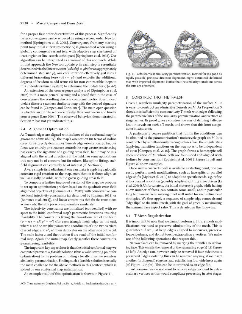
An example result of this optimization is shown in Figure 11.
Fig. 11. Le�: seamless similarity parametrization, rotated for (as good asrigidly possible) principal direction alignment. Right: optimized, deformedmap with improved alignment. Notice that the similarity transitions acrossthe cuts are preserved.
8 CONSTRUCTING THE T-MESHGiven a seamless similarity parametrization of the surface M , it
is easy to construct an admissible T-mesh on M . As Proposition 3
shows, it is su�cient to construct any T-mesh with edges following
the parametric lines of the similarity parametrization and vertices at
singularities. Its proof gives a constructive way of de�ning halfedge
knot intervals on such a T-mesh, and shows that this knot assign-
ment is admissible.
A particularly coarse partition that ful�lls the conditions can
be obtained as the parametrization’s motorcycle graph on M . It is
constructed by simultaneously tracing isolines from the singularities
(applying transition functions on the way so as to be independent
of cuts) [Campen et al. 2015]. The graph forms a homotopic cell
decomposition of M , whose cells are four-sided and aligned with
isolines by construction [Eppstein et al. 2008]. Figure 14 left and
Figure 20 show examples.
Once such a coarse T-mesh is available as starting point, one can
easily perform mesh modi�cations, such as face splits or parallel
edge shifts [Myles et al. 2010] to adapt it to speci�c needs, e.g. re�ne
it to a desired resolution (possibly adaptively, �tting error driven [Li
et al. 2006]). Unfortunately, the initial motorcyle graph, while having
a low number of faces, can contain some small, and in particular
long but narrow faces, making it not well suited for such re�nement
strategies. We thus apply a sequence of simple edge removals and
“edge �ips” to the initial mesh, with the goal of greedily maximizing
the minimal face aspect ratio. This is detailed in the following.
8.1 T-Mesh RegularizationIt is important to note that we cannot perform arbitrary mesh mod-
i�cations; we need to preserve admissibility of the mesh. This is
guaranteed if we just keep edges aligned to isocurves, preserve
four-sidedness, and do not touch extraordinary vertices. We make
use of the following operations that respect this.
Narrow faces can be removed by merging them with a neighbor-
ing face. This entails the removal of the separating edge(s) (cf. Figure
12 left). An edge can, however, only be removed if four-sidedness is
preserved. Edges violating this can be removed anyway, if we insert
another (orthogonal) edge instead, establishing four-sidedness again
(cf. Figure 12 right). This can be interpreted as an edge �ip.
Furthermore, we do not want to remove edges incident to extra-
ordinary vertices as this would complicate processing in later stages.
ACM Transactions on Graphics, Vol. 36, No. 4, Article 91. Publication date: July 2017.
Similarity Maps and Field-Guided T-Splines: a Perfect Couple • 91:11
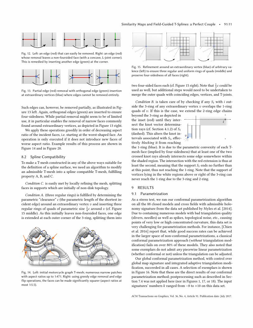
Fig. 12. Le�: an edge (red) that can easily be removed. Right: an edge (red)whose removal leaves a non-foursided face (with a concave, L-joint corner).This is remedied by inserting another edge (green) at the corner.
Fig. 13. Partial edge (red) removal with orthogonal edge (green) insertionat extraordinary vertices (blue) where edges cannot be removed entirely.
Such edges can, however, be removed partially, as illustrated in Fig-
ure 13 left. Again, orthogonal edges (green) are inserted to ensure
four-sidedness. While partial removal might seem to be of limited
use, it in particular enables the removal of narrow faces commonly
found around extraordinary vertices, as depicted in Figure 13 right.
We apply these operations greedily in order of decreasing aspect
ratio of the incident faces, i.e. starting at the worst-shaped face. An
operation is only executed if it does not introduce new faces of
worse aspect ratio. Example results of this process are shown in
Figure 14 and in Figure 20.
8.2 Spline CompatibilityTo make a T-mesh constructed in any of the above ways suitable for
the de�nition of a spline surface, we need an algorithm to modify
an admissible T-mesh into a spline compatible T-mesh, ful�lling
property A, B, and C.
Condition C. is easily met by locally re�ning the mesh, splitting
faces in supports which are initially of non-disk topology.
Condition A. (three regular rings) is ful�lled by determining the
parametric “clearance” c (the parametric length of the shortest in-
cident edge) around an extraordinary vertex v and inserting three
regular rings of quads of parametric size1
4c around v (cf. Figure
15 middle). As this initially leaves non-foursided faces, one edge
is extended at each outer corner of the 3-ring, splitting them into
Fig. 14. Le�: initial motorcycle graph T-mesh; numerous narrow patcheswith aspect ratios up to 1:471. Right: using greedy edge removal and edgeflip operations, the faces can be made significantly squarer (aspect ratios atmost 1:5.5).
Fig. 15. Refinement around an extraordinary vertex (blue) of arbitrary va-lence (le�) to ensure three regular and uniform rings of quads (middle) andpreserve four-sidedness of all faces (right).
two four-sided faces each (cf. Figure 15 right). Note that1
3c could be
used as well, but additional steps would need to be undertaken to
merge the outer quads with coinciding edges, vertices, and T-joints.
Condition B. is taken care of by checking if any Si with i out-
side the 3-ring of any extraordinary vertex v overlaps the 1-ring
quads of v . If this is the case, we extend the 2-ring edge chains
v
i
beyond the 3-ring as depicted in
the inset (red) until they inter-
sect the knot vector determina-
tion rays (cf. Section 4.1.2) of Si(dashed). This alters the knot in-
tervals associated with Si , e�ec-
tively blocking it from reaching
the 1-ring (blue). It is due to the parametric convexity of each T-
mesh face (implied by four-sidedness) that at least one of the two
crossed knot rays already intersects some edge somewhere within
the shaded region. The intersection with the red extension is thus at
least the second, meaning that the support Si ends no further than
at this point, thus not reaching the 1-ring. Note that the support of
vertices lying in the white regions above or right of the 3-ring can
never reach the 1-ring due to the 3-ring and 2-ring.
9 RESULTS
9.1 ParametrizationAs a stress test, we ran our conformal parametrization algorithm
on all the 88 closed models and cross �elds with admissible holo-
nomy signature from the data set published by Myles et al. [2014].
Due to containing numerous models with bad triangulation quality
(slivers, needles) as well as spikes, topological noise, etc., causing
points of very low or high concentrated curvature, this data set is
very challenging for parametrization methods. For instance, [Chien
et al. 2016] report that, while good success rates can be achieved
in the larger space of non-conformal parametrizations, a classical
conformal parametrization approach (without triangulation mod-
i�cation) fails on over 80% of these models. They also noted that
some exemplars do not admit any piecewise linear parametrization
(whether conformal or not) unless the triangulation can be adjusted.
Our global conformal parametrization method, with control over
global map signature and integrated adaptive triangulation modi-
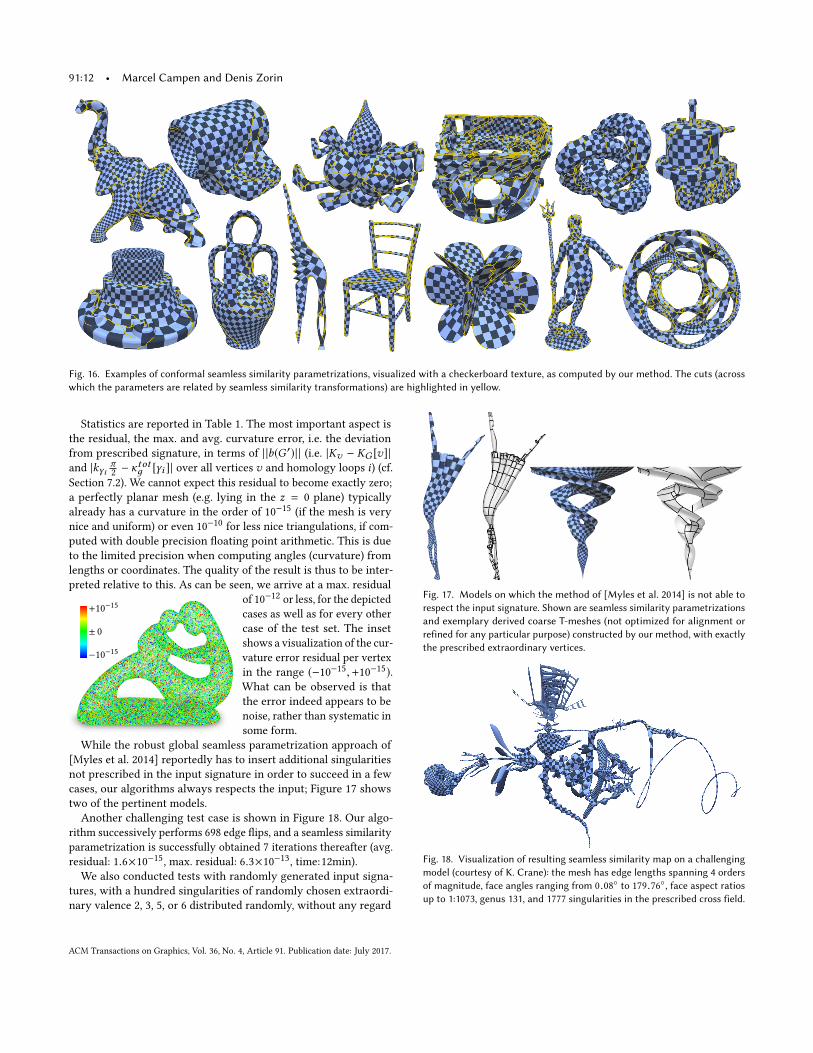
�cation, succeeded in all cases. A selection of exemplars is shown
in Figure 16. Note that these are the direct results of our conformal
parametrization method; postprocessing such as described in Sec-
tion 7.4 was not applied here (nor in Figures 1, 17, or 18). The input
signatures’ numbers k ranged from −8 to +10 on this data set.
ACM Transactions on Graphics, Vol. 36, No. 4, Article 91. Publication date: July 2017.
91:12 • Marcel Campen and Denis Zorin
Fig. 16. Examples of conformal seamless similarity parametrizations, visualized with a checkerboard texture, as computed by our method. The cuts (acrosswhich the parameters are related by seamless similarity transformations) are highlighted in yellow.
Statistics are reported in Table 1. The most important aspect is
the residual, the max. and avg. curvature error, i.e. the deviation
from prescribed signature, in terms of | |b(G ′)| | (i.e. |Kv − KG [v]|and |kγi
π2− κtotд [γi ]| over all vertices v and homology loops i) (cf.
Section 7.2). We cannot expect this residual to become exactly zero;
a perfectly planar mesh (e.g. lying in the z = 0 plane) typically
already has a curvature in the order of 10−15
(if the mesh is very
nice and uniform) or even 10−10
for less nice triangulations, if com-
puted with double precision �oating point arithmetic. This is due
to the limited precision when computing angles (curvature) from
lengths or coordinates. The quality of the result is thus to be inter-
preted relative to this. As can be seen, we arrive at a max. residual
−10−15
± 0
+10−15of 10
−12or less, for the depicted
cases as well as for every other
case of the test set. The inset
shows a visualization of the cur-
vature error residual per vertex
in the range (−10−15,+10−15).
What can be observed is that
the error indeed appears to be
noise, rather than systematic in
some form.
While the robust global seamless parametrization approach of
[Myles et al. 2014] reportedly has to insert additional singularities
not prescribed in the input signature in order to succeed in a few
cases, our algorithms always respects the input; Figure 17 shows
two of the pertinent models.
Another challenging test case is shown in Figure 18. Our algo-
rithm successively performs 698 edge �ips, and a seamless similarity
parametrization is successfully obtained 7 iterations thereafter (avg.
residual: 1.6×10⁻¹⁵, max. residual: 6.3×10⁻¹³, time:12min).
We also conducted tests with randomly generated input signa-
tures, with a hundred singularities of randomly chosen extraordi-
nary valence 2, 3, 5, or 6 distributed randomly, without any regard
Fig. 17. Models on which the method of [Myles et al. 2014] is not able torespect the input signature. Shown are seamless similarity parametrizationsand exemplary derived coarse T-meshes (not optimized for alignment orrefined for any particular purpose) constructed by our method, with exactlythe prescribed extraordinary vertices.
Fig. 18. Visualization of resulting seamless similarity map on a challengingmodel (courtesy of K. Crane): the mesh has edge lengths spanning 4 ordersof magnitude, face angles ranging from 0.08◦ to 179.76◦, face aspect ratiosup to 1:1073, genus 131, and 1777 singularities in the prescribed cross field.
ACM Transactions on Graphics, Vol. 36, No. 4, Article 91. Publication date: July 2017.
Similarity Maps and Field-Guided T-Splines: a Perfect Couple • 91:13
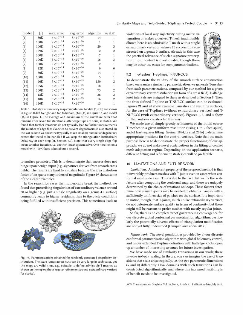
model |F | max. error avg. error edge�ips w/ iDT
(1) 50K 6×10⁻¹⁴ 8×10⁻¹⁶ 14 1
(2) 100K 2×10⁻¹⁴ 7×10⁻¹⁶ 1 1
(3) 100K 9×10⁻¹⁵ 7×10⁻¹⁶ 20 3
(4) 129K 2×10⁻¹⁴ 7×10⁻¹⁶ 2 2
(5) 100K 4×10⁻¹⁴ 1×10⁻¹⁵ 7 1
(6) 100K 5×10⁻¹⁴ 8×10⁻¹⁶ 16 3
(7) 100K 9×10⁻¹⁵ 7×10⁻¹⁶ 2 1
(8) 82K 6×10⁻¹⁵ 6×10⁻¹⁶ 0 0
(9) 50K 3×10⁻¹⁴ 8×10⁻¹⁶ 14 1
(10) 100K 2×10⁻¹⁴ 8×10⁻¹⁶ 5 1
(11) 20K 5×10⁻¹³ 3×10⁻¹⁵ 180 2
(12) 105K 5×10⁻¹³ 8×10⁻¹⁵ 18 1
(13) 100K 3×10⁻¹³ 1×10⁻¹⁵ 75 2
(14) 18K 2×10⁻¹⁴ 9×10⁻¹⁶ 26 2
(15) 10K 3×10⁻¹³ 1×10⁻¹⁵ 16 2
(16) 120K 5×10⁻¹⁴ 7×10⁻¹⁶ 13 1
Table 1. Statistics of similarity map computation. Models (1)-(13) are shownin Figure 16 le� to right and top to bo�om, (14)-(15) in Figure 17, and model(16) in Figure 1. The average and maximum of the curvature error thatremains a�er seven full iterations (a�er edge flips are done) is stated. Wefound that further iterations do not typically lead to further improvements.The number of edge flips executed to prevent degeneracies is also stated. Inthe last column we show the (typically much smaller) number of degeneracyevents that need to be handled if we keep the triangulation intrinsicallyDelaunay at each step (cf. Section 7.3). Note that every single edge flipincurs another iteration, i.e. another linear system solve. One iteration on amodel with 100K faces takes about 1 second.
to surface geometry. This is to demonstrate that success does not
hinge upon benign input (e.g. signatures derived from smooth cross
�elds). The results are hard to visualize because the area distortion
factor often spans many orders of magnitude; Figure 19 shows some
of the clearer examples.
In the search for cases that numerically break the method, we
found that prescribing singularities of extraordinary valence around
30 or higher (e.g. just a single singularity on a genus 4+ surface)
commonly leads to higher residuals, thus to the cycle conditions
being ful�lled with insu�cient precision. This sometimes leads to
Fig. 19. Parametrizations obtained for randomly generated singularity dis-tributions. The scale jumps across cuts can be very large in such cases, yetthe maps are valid, thus, e.g., suitable to define admissible T-meshes asshown on the top (without regular refinement around extraordinary verticesfor clarity).
violations of local map injectivity during metric in-
tegration or makes a derived T-mesh inadmissible.
Shown here is an admissible T-mesh with a single
extraordinary vertex of valence 20 successfully con-
structed on a genus 3 surface. Already in this case
the practical relevance of such a signature prescrip-
tion in our context is questionable, though there
may be other use cases for such parametrizations.
9.2 T-Meshes, T-Splines, T-NURCCSTo demonstrate the validity of the smooth surface construction
based on seamless similarity parametrization, we generate T-meshes
from such parametrizations, computed by our method for a given
extraordinary vertex distribution (in form of a cross �eld). Halfedge
knot intervals are assigned to these as described in Section 8. Then
the thus de�ned T-spline or T-NURCC surface can be evaluated.
Figures 21 and 20 show example T-meshes and resulting surfaces,
for the case of T-splines (without extraordinary vertices) and T-
NURCCS (with extraordinary vertices). Figures 1, 5, and 4 show
further surfaces constructed this way.
We made use of simple greedy re�nement of the initial coarse
T-meshes to a given uniform resolution (using 1-to-2 face splits),
and of least-squares �tting [Greiner 1994; Li et al. 2006] to determine
appropriate positions for the control vertices. Note that the main
purpose here is to demonstrate the proper functioning of our ap-
proach; we do not make novel contributions in the �tting or control
mesh adaptation regime. Depending on the application scenario,
di�erent �tting and re�nement strategies will be preferable.
10 LIMITATIONS AND FUTURE WORKLimitations. An inherent property of the proposed method is that
it invariably produces meshes with T-joints even in cases when con-
formal meshes do exist. This is due to the fact that we �x the scale
factors after computing the conformal map, and these are uniquely
determined by the choice of rotations on loops. These factors deter-
mine how many T-joints may be needed to obtain a T-mesh with a
su�ciently uniform size of patches on the surface. It is important
to notice, though, that T-joints, much unlike extraordinary vertices,
do not deteriorate surface quality in terms of continuity, but there
might still be reasons to prefer meshes with mostly regular joints.
So far, there is no complete proof guaranteeing convergence for
our discrete global conformal parametrization algorithm; particu-
larly the potentially adverse e�ects of triangulation modi�cation
are not yet fully understood [Campen and Zorin 2017].
Future work. The novel possibilities provided by a) our discrete
conformal parametrization algorithm with global holonomy control,
and b) our extended T-spline de�nition with halfedge knots, open
up a number of interesting avenues for future investigation.
We have made use of similarity transitions in our work; these
involve isotropic scaling. In theory, one can imagine the use of tran-
sitions that scale anisotropically, i.e. the two parametric dimensions
(u and v) di�erently. How domains with such transitions can be
constructed algorithmically, and where this increased �exibility is
of bene�t needs to be investigated.
ACM Transactions on Graphics, Vol. 36, No. 4, Article 91. Publication date: July 2017.
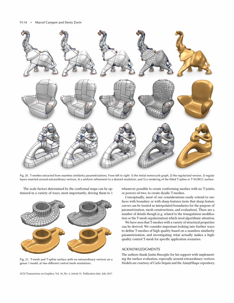
91:14 • Marcel Campen and Denis Zorin
Fig. 20. T-meshes extracted from seamless similarity parametrizations. From le� to right: 1) the initial motorcycle graph, 2) the regularized version, 3) regularlayers inserted around extraordinary vertices, 4) a uniform refinement to a desired resolution, and 5) a rendering of the fi�ed T-spline or T-NURCC surface.
The scale factors determined by the conformal maps can be op-
timized in a variety of ways, most importantly, driving them to 1
Fig. 21. T-mesh and T-spline surface with no extraordinary vertices on agenus 1 model, at two di�erent control mesh resolutions.
whenever possible to create conforming meshes with no T-joints,
or powers-of-two, to create dyadic T-meshes.
Conceptually, most of our considerations easily extend to sur-
faces with boundary or with sharp features (note that sharp feature
curves can be treated as interpolated boundaries for the purpose of
parametrization, mesh constructions, and evaluation). There are a
number of details though (e.g. related to the triangulation modi�ca-
tion or the T-mesh regularization) which need algorithmic attention.
We have seen that T-meshes with a variety of structural properties
can be derived. We consider important looking into further ways
to de�ne T-meshes of high quality based on a seamless similarity
parametrization, and investigating what actually makes a high-
quality control T-mesh for speci�c application scenarios.
ACKNOWLEDGMENTSThe authors thank Justin Bisceglio for his support with implement-
ing the surface evaluation, especially around extraordinary vertices.
Models are courtesy of Carlo Séquin and the Aim@Shape repository.
ACM Transactions on Graphics, Vol. 36, No. 4, Article 91. Publication date: July 2017.
Similarity Maps and Field-Guided T-Splines: a Perfect Couple • 91:15
REFERENCESRalph Abraham, Jerrold E Marsden, and Tudor Ratiu. 1988. Manifolds, Tensor Analysis,
and Applications. Springer, New York, NY, USA.
Noam Aigerman and Yaron Lipman. 2015. Orbifold Tutte Embeddings. ACM Trans.Graph. 34, 6 (2015), 190:1–190:12.
Pierre Alliez, David Cohen-Steiner, Olivier Devillers, Bruno Lévy, and Mathieu Desbrun.
2003. Anisotropic polygonal remeshing. ACM Trans. Graph. 22, 3 (2003).
Thierry Aubin. 1998. Some Nonlinear Problems in Riemannian Geometry. Springer
Berlin Heidelberg.
Yuri Bazilevs, Victor M Calo, John A Cottrell, John A Evans, TJR Hughes, S Lipton,
Michael A Scott, and Thomas W Sederberg. 2010. Isogeometric analysis using
T-splines. Computer Methods in Applied Mechanics and Eng. 199, 5 (2010), 229–263.
Mirela Ben-Chen, Craig Gotsman, and Guy Bunin. 2008. Conformal �attening by
curvature prescription and metric scaling. In Comp. Graph. Forum, Vol. 27. 449–458.
Martin Bertram, Mark A. Duchaineau, Bernd Hamann, and Kenneth I. Joy. 2004. Gen-
eralized B-Spline Subdivision-Surface Wavelets for Geometry Compression. IEEETVCG 10, 3 (2004), 326–338.
Ioana Boier-Martin, Holly Rushmeier, and Jingyi Jin. 2004. Parameterization of triangle
meshes over quadrilateral domains. Symp. on Geometry Processing (2004), 193–203.
David Bommes, Marcel Campen, Hans-Christian Ebke, Pierre Alliez, and Leif Kobbelt.
2013. Integer-grid maps for reliable quad meshing. ACM Trans. Graph. 32, 4 (2013).
David Bommes, Henrik Zimmer, and Leif Kobbelt. 2009. Mixed-integer quadrangulation.
ACM Trans. Graph. 28, 3 (2009), 77.
Philip L. Bowers and Monica K. Hurdal. 2003. Planar Conformal Mappings of PiecewiseFlat Surfaces. Springer Berlin Heidelberg, 3–34.
Guy Bunin. 2008. A continuum theory for unstructured mesh generation in two
dimensions. Computer Aided Geometric Design 25, 1 (2008), 14–40.
Marcel Campen, David Bommes, and Leif Kobbelt. 2015. Quantized global parametriza-
tion. ACM Trans. Graph. 34, 6 (2015), 192.
Marcel Campen and Leif Kobbelt. 2014. Quad Layout Embedding via Aligned Parame-
terization. Comp. Graph. Forum 33, 8 (2014).
Marcel Campen and Denis Zorin. 2017. On Discrete Conformal Seamless Similarity
Maps. (2017). arXiv:1705.02422
Nathan A. Carr, Jared Hoberock, Keenan Crane, and John C. Hart. 2006. Rectangular
multi-chart geometry images. In Proc. SGP ’06. 181–190.
Thomas J. Cashman. 2012. Beyond Catmull-Clark? A Survey of Advances in Subdivision
Surface Methods. Comp. Graph. Forum 31, 1 (2012), 42–61.
Edward Chien, Zohar Levi, and O�r Weber. 2016. Bounded Distortion Parametrization
in the Space of Metrics. ACM Trans. Graph. 35, 6 (2016), 215:1–215:16.
Bennett Chow and Feng Luo. 2003. Combinatorial Ricci Flows on Surfaces. J. Di�erentialGeom. 63, 1 (2003), 97–129.
Keenan Crane, Mathieu Desbrun, and Peter Schröder. 2010. Trivial Connections on
Discrete Surfaces. Comp. Graph. Forum 29, 5 (2010), 1525–1533.
Jiansong Deng, Falai Chen, Xin Li, Changqi Hu, Weihua Tong, Zhouwang Yang, and
Yuyu Feng. 2008. Polynomial Splines over Hierarchical T-meshes. Graph. Models 70,
4 (2008), 76–86.
Mathieu Desbrun, Eva Kanso, and Yiying Tong. 2008. Discrete Di�erential Forms forComputational Modeling. Birkhäuser Basel, 287–324.
Hans-Christian Ebke, Patrick Schmidt, Marcel Campen, and Leif Kobbelt. 2016. Inter-
actively Controlled Quad Remeshing of High Resolution 3D Models. ACM Trans.Graph. 35, 6 (2016), 218:1–218:13.
Matthias Eck and Hugues Hoppe. 1996. Automatic Reconstruction of B-spline Surfaces
of Arbitrary Topological Type. In Proc. (SIGGRAPH ’96). 325–334.
David Eppstein, Michael T. Goodrich, Ethan Kim, and Rasmus Tamstorf. 2008. Motor-
cycle Graphs: Canonical Quad Mesh Partitioning. Comp. Graph. Forum 27, 5 (2008),
1477–1486.
Gerald Farin. 2002. Curves and Surfaces for CAGD: A Practical Guide (5th ed.). Morgan
Kaufmann Publishers Inc., San Francisco, CA, USA.
Matthew Fisher, Boris Springborn, Peter Schröder, and Alexander I Bobenko. 2007. An
algorithm for the construction of intrinsic Delaunay triangulations with applications
to digital geometry processing. Computing 81, 2-3 (2007), 199–213.
Gunther Greiner. 1994. Variational Design and Fairing of Spline Surfaces. Comp. Graph.Forum 13, 3 (1994).
Xianfeng Gu, Ying He, Miao Jin, Feng Luo, Hong Qin, and Shing-Tung Yau. 2008.
Manifold splines with a single extraordinary point. Computer-Aided Design 40, 6
(2008), 676–690.
Xianfeng Gu, Feng Luo, Jian Sun, and Tianqi Wu. 2013. A discrete uniformization
theorem for polyhedral surfaces. arXiv:1309.4175 (2013).
Xianfeng Gu and Shing-Tung Yau. 2003. Global conformal surface parameterization. In
Proc. Symposium on Geometry Processing 2003. 127–137.
Ying He, Kexiang Wang, Hongyu Wang, Xianfeng Gu, and Hong Qin. 2006. Manifold
T-Spline. In Proc. Geometric Modeling and Processing. 409–422.
Miao Jin, Junho Kim, and Xianfeng David Gu. 2007. Discrete Surface Ricci Flow: Theoryand Applications. 209–232.
Ernest Jucovič and Marián Trenkler. 1973. A theorem on the structure of cell–
decompositions of orientable 2–manifolds. Mathematika 20, 01 (1973), 63–82.
Felix Kälberer, Matthias Nieser, and Konrad Polthier. 2007. QuadCover: Surface Param-
eterization using Branched Coverings. Comp. Graph. Forum 26, 3 (2007), 375–384.
Kestutis Karciauskas, Daniele Panozzo, and Jörg Peters. 2016. Spline surfaces with
T-junctions. (2016). arXiv:1610.05351.
Liliya Kharevych, Boris Springborn, and Peter Schröder. 2006. Discrete Conformal
Mappings via Circle Patterns. ACM Trans. Graph. 25, 2 (2006), 412–438.
Andrei Khodakovsky, Peter Schröder, and Wim Sweldens. 2000. Progressive Geometry
Compression. In Proc. SIGGRAPH ’00. 271–278.
Denis Kovacs, Justin Bisceglio, and Denis Zorin. 2015. Dyadic T-mesh Subdivision.
ACM Trans. Graph. 34, 4 (2015), 143:1–143:12.
Wan-Chiu Li, Nicolas Ray, and Bruno Lévy. 2006. Automatic and interactive mesh to
T-spline conversion. In Proc. SGP ’06. 191–200.
Xin Li, Jiansong Deng, and Falai Chen. 2010. Polynomial splines over general T-meshes.
The Visual Computer 26, 4 (2010), 277–286.
Xin Li, G. Thomas Finnigan, and Thomas W. Sederberg. 2016. G1 Non-uniform Catmull-
Clark Surfaces. ACM Trans. Graph. 35, 4 (2016), 135:1–135:8.
Xin Li, Jianmin Zheng, Thomas W. Sederberg, Thomas J. R. Hughes, and Michael A.
Scott. 2012. On linear independence of T-spline blending functions. Computer AidedGeometric Design 29, 1 (2012), 63–76.
Yaron Lipman. 2012. Bounded distortion mapping spaces for triangular meshes. ACMTrans. Graph. 31, 4 (2012), 108.
Michael Lounsbery, Tony D. DeRose, and Joe Warren. 1997. Multiresolution Analysis
for Surfaces of Arbitrary Topological Type. ACM Trans. Graph. 16, 1 (1997), 34–73.
Feng Luo. 2004. Combinatorial Yamabe �ow on surfaces. Communications in Contem-porary Mathematics 6, 05 (2004), 765–780.
Kerstin Müller, Lars Reusche, and Dieter Fellner. 2006. Extended Subdivision Surfaces:
Building a Bridge Between NURBS and Catmull-Clark Surfaces. ACM Trans. Graph.25, 2 (2006), 268–292.
Ashish Myles, Nico Pietroni, Denis Kovacs, and Denis Zorin. 2010. Feature-aligned
T-meshes. ACM Trans. Graph. 29, 4 (2010), 117:1–117:11.
Ashish Myles, Nico Pietroni, and Denis Zorin. 2014. Robust Field-aligned Global
Parametrization. ACM Trans. Graph. 33, 4 (2014).
Ashish Myles and Denis Zorin. 2012. Global parametrization by incremental �attening.
ACM Trans. Graph. 31, 4 (2012), 109.
Ashish Myles and Denis Zorin. 2013. Controlled-distortion constrained global
parametrization. ACM Trans. Graph. 32, 4 (2013), 105.
Daniele Panozzo, Enrico Puppo, Marco Tarini, Nico Pietroni, and Paolo Cignoni. 2011.
Automatic Construction of Quad-Based Subdivision Surfaces Using Fitmaps. IEEETransactions on Visualization and Computer Graphics 17, 10 (2011), 1510–1520.
Jörg Peters. 1992. Joining smooth patches around a vertex to form a Cksurface.
Computer Aided Geometric Design 9, 5 (1992), 387 – 411.
M. M. Postnikov. 2001. Geometry VI: Riemannian Geometry. Springer Berlin Heidelberg.
Nicolas Ray, Wan Chiu Li, Bruno Lévy, Alla She�er, and Pierre Alliez. 2006. Periodic
Global Parameterization. ACM Trans. Graph. 25, 4 (2006), 1460–1485.
Nicolas Ray, Vincent Nivoliers, Sylvain Lefebvre, and Bruno Lévy. 2010. Invisible Seams.
In Proc. Eurographics Symposium on Rendering.
Nicolas Ray and Dmitry Sokolov. 2014. Robust Polylines Tracing for N-Symmetry
Direction Field on Triangulated Surfaces. ACM Trans. Graph. 33, 3 (2014).
Nicolas Ray, Bruno Vallet, Wan Chiu Li, and Bruno Lévy. 2008. N-Symmetry direction
�eld design. ACM Trans. Graph. 27 (2008), 2.
Richard Schoen and Shing-Tung Yau. 1994. Lectures on Di�erential Geometry. Interna-
tional Press.
Thomas W. Sederberg, David L. Cardon, G. Thomas Finnigan, Nicholas S. North, Jianmin
Zheng, and Tom Lyche. 2004. T-spline Simpli�cation and Local Re�nement. ACMTrans. Graph. 23, 3 (2004), 276–283.
Thomas W. Sederberg, G. Thomas Finnigan, Xin Li, Hongwei Lin, and Heather Ipson.
2008. Watertight trimmed NURBS. ACM Trans. Graph. 27, 3 (2008).
Thomas W. Sederberg, Jianmin Zheng, Almaz Bakenov, and Ahmad Nasri. 2003. T-
splines and T-NURCCs. ACM Trans. Graph. 22, 3 (2003), 477–484.
Boris Springborn, Peter Schröder, and Ulrich Pinkall. 2008. Conformal equivalence of
triangle meshes. ACM Trans. Graph. 27, 3 (2008).
Jos Stam. 1998. Exact Evaluation of Catmull-Clark Subdivision Surfaces at Arbitrary
Parameter Values. In Proc (SIGGRAPH ’98). 395–404.
Yiying Tong, Pierre Alliez, Daniel Cohen-Steiner, and Mathieu Desbrun. 2006. Designing
quadrangulations with discrete harmonic forms. Symposium on Geometry Processing(2006), 201–210.
Marc Troyanov. 1991. Prescribing curvature on compact surfaces with conical singular-
ities. Trans. Amer. Math. Soc. 324 (1991), 793–821.
Amir Vaxman, Marcel Campen, Olga Diamanti, Daniele Panozzo, David Bommes, Klaus
Hildebrandt, and Mirela Ben-Chen. 2016. Directional Field Synthesis, Design, and
Processing. Comp. Graph. Forum 35, 2 (2016).
Wenyan Wang, Yongjie Zhang, Guoliang Xu, and ThomasJ.R. Hughes. 2012. Converting
an unstructured quadrilateral/hexahedral mesh to a rational T-spline. ComputationalMechanics 50, 1 (2012), 65–84.
Denis Zorin, Peter Schröder, and Wim Sweldens. 1997. Interactive Multiresolution
Mesh Editing. In Proc. SIGGRAPH ’97. 259–268.
ACM Transactions on Graphics, Vol. 36, No. 4, Article 91. Publication date: July 2017.
91:16 • Marcel Campen and Denis Zorin
A PROOFS
Proof of Proposition 1Proof. The invariance of F to seamless similarity transforms
applied to domains and knot vectors is a direct consequence of the
invariance of each basis function to such transforms, as established
by Proposition 2. As knot vectors are determined with respect to the
local systems in D, and these local systems di�er between di�erent
choices of anchor quads by seamless similarity transforms only
(namely compositions of τ [Fm , Fn ] and translations, all of which are
seamless similarity transforms), F is in particular invariant to the
choice of anchor quads and local coordinate systems. As a special
case, this implies that the quadrant basis functions of one basis
functions, even if de�ned with respect to individual anchors, thus
di�erent local systems, join in a C2(or “G2
”) manner, just as if they
were de�ned with respect to the same system, thus were simply
restrictions of the same function.
Continuity orderC2of F away from extraordinary points follows
from the C2continuity of each basis function (composed of quad-
rants) and all applied transforms τ [F ,D] being smooth similarity
transformations. F is piecewise rational, away from extraordinary
points, because the underlying construction of T-splines (1) yields
piecewise rational functions [Sederberg et al. 2003]. �
Proof of Proposition 2Proof. Indeed, nontrivial rotations by kπ/2 are a combination of
�ipping the signs of knots with possibly switchingu andv directions,
with ui = ±sui + tu or ui = ±svi + tu . Consider one of the one-
dimensional factors B[u](u) in the formula. Clearly, for a spline of
order 0, the proposition holds. Next, we substitute the transform
formulas into the recursive de�nition:
Bi,k (u) =u − ui
ui+k−1 − uiBi,k−1(u) +
ui+k − u
ui+k − ui+1Bi+1,k−1(u),
where the i-th basis function is supported on ui , . . . ,ui+k .
If u and v are not switched, we observe that the coe�cients
of the formula are invariant with respect to the transformation:
u′−u′iu′i+k−1−u
′i=
u−uiui+k−1−ui
, and we conclude that B[u′](u ′) = B(u)(u) by
induction on order. The same holds for B[v]. If u and v are switched
by the rotation, in a similar way we observe that B[u′](u ′) = B[v](v)and B[v′](v ′) = B[u](u). As B[u′, v′](u′, v′) = B[u′](u ′)B[v′](v ′),this yields the formula in the proposition. �
Proof of Proposition 4Proof. It remains to show that the conformal map f is a seamless
similarity map, i.e. the transition functions across cuts are similar-
ities that are constant on each branch (segment not containing a
singularity or branching point) of the cut graph.
As ξ = ?ωf , de�ned on M , is continuous on the cut, we have
dϕc1= ξ = dϕc
2, where ϕci are the two values of ϕ on di�erent sides
of the cut. Integrating along the cut, we see that the changes of
ϕc1
and ϕc2
between two points p and q on a cut branch are the
same, i.e. ϕc1(q) −ϕc
1(p) = ϕc
2(q) −ϕc
2(p). From this we conclude that
ϕc1(q) − ϕc
2(q) = ϕc
1(p) − ϕc
2(p), i.e. jumps in ϕc at di�erent points
p and q on a branch are the same, i.e. the ratio of the scale factors
eϕc1 /eϕ
c2 is constant along a branch.
Concerning the rotational part, consider Df1[p] and Df2[p], the
di�erentials of the map f on the two di�erent sides of the cut at
a point p on the cut, and a loop γ that crosses the cut once at p.
As ωf measures the rate of rotation of the cross �eld de�ned by
Df −1(e1), and as its integral over any loop γ cancels its geodesic
curvature up to a multiple of π/2 by construction of f , the rota-
tion between Df −12[p](e1) and Df −1
1[p](e1) is a multiple of π/2, i.e.
Df −12[p](e1) = sRD f −1
1[p](e1), where R is a rotation by a multiple
of π/2. Note that Df (and thus Df −1) is a rotation + uniform scale
for a �xed pair of coordinate systems on the tangent plane and in the
parametric domain. De�ning a rotation + uniform scale transform
on a single vector (e1) completely determines it, so we conclude that
Df −12[p] = sRD f −1
1[p]. As two-dimensional rotations commute, we
obtain Df −12[p]Df1[p] = sR, i.e. the di�erential of the transition
map from one side of the cut to the other is a kπ/2 rotation com-
posed with a uniform scale. As the rotation along the loop depends
on the regular homotopy class of the loop only, at all points of the
cut branch, the rotation and thus the di�erential of the map is the
same.
Finally, concerning the translational part, integrating di�erentials
from a point on a cut branch to any other point along the branch
by the same argument used for ϕ, we arrive at the conclusion that
the transitions per cut branch are constant similarity maps. �
B INDICATOR FUNCTIONConsider the function I ′i j,k (λ) =
`jke(ϕj (λξ )+ϕk (λξ ))/2+ `kie
(ϕk (λξ )+ϕi (λξ ))/2− `i je(ϕi (λξ )+ϕj (λξ ))/2.
It is a sum of (negated) edge lengths at time λ of the metric
evolution. It is negative if the triangle inequality of triangle ijk is
violated by edge ij being too long, vanishes if edge ij is as long as
the other two edges combined, and positive otherwise. It thus has
the desired degeneracy-indicating behavior. Division by the strictly
positive (thus root preserving) term e(ϕi (λξ )+ϕj (λξ ))/2 yields (9):
`jke(ϕk (ξ )−ϕi (ξ ))λ/2+ `kie
(ϕk (ξ )−ϕj (ξ ))λ/2− `i j = Ii j,k (λ),
using ϕi (ξ ) − ϕ j (ξ ) = ξ ji for any two adjacent vertices i, j. No-
tice that Ii j,k can be evaluated locally directly based on ξ ; global
integration to obtain ϕ is not required.
Furthermore, the second derivative of (9) is strictly positive
d2
dλ2 Ii j,k = `jk1
4ξ 2ike
ξik λ/2 + `ki1
4ξ 2jke
ξ jk λ/2 > 0,
assuming that ξik , 0 or ξ jk , 0 (otherwise the corresponding
triangle remains constant and does not need to be checked for
degeneracy events anyway). This is due to `jk and `ki being positive
by construction. Thus I has at most two roots.
ACM Transactions on Graphics, Vol. 36, No. 4, Article 91. Publication date: July 2017.