Embed Size (px)
Citation preview
SIMGRO V7.1.0User's guide
P.E.V. van Walsum
Alterra-Report 913.2 ISSN 1566-7197


SIMGRO V7.1.0 User's guide

SIMGRO V7.1.0
User’s guide
P.E.V. van Walsum
Alterra Report 913.2
Alterra, Green World Research, Wageningen
© 2010 Alterra,P.O. Box 47, NL-6700 AA Wageningen (The Netherlands).Phone: +31 317 474700; fax: +31 317 419000; e-mail: [email protected]
No part of this publication may be reproduced or published in any form or by any means,or stored in a data base or retrieval system, without the written permission of Alterra.
Alterra assumes no liability for any losses resulting from the use of this document.
ABSTRACT
Walsum, P.E.V. van, 2010. SIMGRO, User’s guide V7.1.0. Wageningen, Alterra.Alterra-Report 913.2. 82 pp.
The regional hydrologic model SIMGRO is used for investigating various kinds ofwater management problems. The model implementation can include the cropgrowth model WOFOST, with feedback to the hydrologic parameters like root zonedepth and leaf area index. SIMGRO is especially suited for modelling situations withshallow groundwater levels in relatively flat areas, like in delta regions. In such terrainthe two-way interaction between groundwater and surface waters plays a crucial role.The offered modelling options include the simulation of drainage with feedback fromsurface water levels at the time step of the ‘fast processes’. The SIMGRO packagealso includes a simplified model for the simulation of surface water processes. Theuser has furthermore the option of through-linking the surface water locations to ahydraulic model. The SIMGRO model assembly for the ‘top system processes’ isused in combination with MODFLOW for the groundwater. This manual containsbrief information regarding the way theoretical concepts relate to practical watermanagement issues, how to set up the model schematization, technical features ofthe modules, installation, program use and error handling.
Keywords: regional hydrology, simulation, water management, crop growth.
ISSN 1566-7197
5
Contents
1 Introduction 9
1.1 Modules and options for links 91.2 Overview of this document 12
2 Input files and model use 13
2.1 Data flow and overview of input files 132.2 Setting up the schematization 15
2.2.1 Coupling in space 152.2.2 Coupling in time 18
2.3 Plant/Soil-Atmosphere interactions 192.3.1 Precipitation 192.3.2 Sprinkling 202.3.3 Interception and interception evaporation 232.3.4 Evapotranspiration 242.3.5 Crop growth simulation 26
2.4 Soil water 272.4.1 Surface runoff 272.4.2 Unsaturated flow 29
2.5 Drainage 312.6 Surface water 33
2.6.1 Watercourses of the regional system 332.6.2 Weirs and pumps 392.6.3 Surface water supply 41
2.7 Time dependency 45
3 Output files 47
3.1 ASCII-output files 473.2 Binary output files 483.3 Extracting data from binary files 49
4 Programme execution 53
4.1 Hardware requirements 534.2 Executables 534.3 MODFLOW-SIMGRO solution scheme parameters 544.4 Problems during execution 55
6
Appendix A PreMetaSWAP 59
1 Program use 59
2 Input file descriptions 61
2.1 COMP_SWAP.CSV 622.2 FEDDES_SWAP.CSV 632.3 TAUFUNC_SWAP.CSV 642.4 HZN_SWAP.CSV 652.5 SPU_SWAP.CSV 662.5 BOX_SWAP.CSV 672.6 ROOTD_SWAP.CSV 692.7 GWL_SWAP.CSV 702.8 QTOP_SWAP.CSV 712.9 TPOT_SWAP.CSV 72
3 Output files 73
Appendix B PostMetaSWAP 75
1 Program use 75
2 Input file descriptions 77
2.1 COMP_POST.CSV 782.2 SEL_SVAT.INP 78
3 Output files 79
Appendix C Demonstration dataset 81
1 T-model_Basic 81
7
PREFACE
In the past year the model has been made suitable for soils with deepgroundwater levels; formerly the evapotranspiration of such soils wasunder¬estimated. The added extra ‘aggregation layer’ for the zone just below theroot zone remedied that deficiency. The idea of using extra aggregation layerswas first suggested by former colleague Pim Dik. This idea has now beenimplemented in a generalized form, involving N-layers forming a cascade ofnonlinear reservoirs.
The second major enhancement of the last year was the coupling to the cropgrowth model WOFOST. This coupling has been implemented in a two-wayfashion, including the (optional) feedback from the vegetation development to thehydrologic model. The used state variables for this feedback are the depth of theroot zone, the crop height, the leaf area index, and the soil cover. For facilitatingthis feedback an option was included for dynamic development of the root zonelayer in MetaSWAP. The coupling to WOFOST coincided with the enhancementof the SWAP-WOFOST coupling by SWAP developers Joop Kroes, Jos van Damand the WOFOST expert Iwan Supit. They provided the information needed forrealizing the coupling of WOFOST to SIMGRO.
The concept for the interception evaporation was reformulated, in collaborationwith the SWAP developers. Furthermore, the SWAP-method for handling thepartitioning between transpiration and soil evaporation was implemented. TheMaas-Hoffman method was included for simulating the effect of salt stress on thetranspiration uptake. The coupling to the TRANSOL model for simulating solutemovements and processes in soils was implemented in collaboration with JoopKroes. The program metaswap2transol also includes the temperature simulationof SWAP.
Low-cost parallel computing is now possible on multi-core pc’s with 2 to 8 cores.And high-performance pc-clusters provide a further multiplication of computingpower. To make use of these opportunities the codes of MetaSWAP andSIMGRO-drainage have been parallelized via the OpenMP-protocol incombination with a state-of-art 64bit-compiler (Intel Fortran 11.1).
SIMGRO has a history that goes back to the mid-eighties. The first and secondversions were developed by Erik Querner in collaboration with Jan van Bakel. Inthe course of time, various other persons not belonging to the current team havecontributed in one way or the other: Pim Dik, Robert Smit, and Frank van derBolt.
The realization of SIMGRO7 was financed by the National Hydrologic Instrumentproject, by the Centre for Water & Climate of Alterra-Wageningen UR, by theAlterra funds for strategic research, and by the GENESIS project of 7th EUFramework program.
Wageningen, December 2009.

Alterra Report 913.2_V7.1.0 9
1 Introduction
Integrated modelling has the attraction of including feedback mechanisms between
the hydrological subsystems. However, covering a wide range of processes in a
spatially distributed manner requires a large logistic effort, involving masses of data.
Even the experienced modeller can easily make a fatal mistake. In the form of an
ultimate safety net, there is of course no substitute for constant awareness and
thorough analysis of the simulation results. However, avoiding mistakes in the first
place is usually more efficient, and one of the prerequisites for doing that is to have a
good overview of the model and its data. At a conceptual level, that overview is
provided by the theory description in Alterra-Report 913.1. In the form of a reference
manual, the formats of input and output files are described in Alterra-Report 913.3.
The latter has the disadvantage that it is purely data-oriented, and not so much
conceptually oriented. The aim of this guide is to document the functionalities at a
technical level, following the thematic overview given in the theory description. It is
hopefully of help in quickly making choices with respect to the modelling options and
in maintaining an overview of a study.
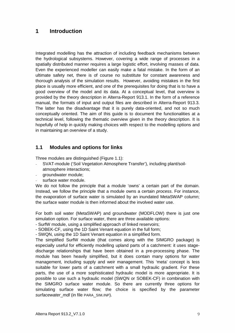
1.1 Modules and options for links
Three modules are distinguished (Figure 1.1):
- SVAT-module (‘Soil Vegetation Atmosphere Transfer’), including plant/soil-
atmosphere interactions;
- groundwater module;
- surface water module.
We do not follow the principle that a module ‘owns’ a certain part of the domain.
Instead, we follow the principle that a module owns a certain process. For instance,
the evaporation of surface water is simulated by an inundated MetaSWAP column;
the surface water module is then informed about the involved water use.
For both soil water (MetaSWAP) and groundwater (MODFLOW) there is just one
simulation option. For surface water, there are three available options:
- SurfW module, using a simplified approach of linked reservoirs;- SOBEK-CF, using the 1D Saint Venant equation in the full form;- SWQN, using the 1D Saint Venant equation in a simplified form.
The simplified SurfW module (that comes along with the SIMGRO package) is
especially useful for efficiently modelling upland parts of a catchment: it uses stage-
discharge relationships that have been obtained in a pre-processing phase. The
module has been heavily simplified, but it does contain many options for water
management, including supply and weir management. This ‘meta’ concept is less
suitable for lower parts of a catchment with a small hydraulic gradient. For these
parts, the use of a more sophisticated hydraulic model is more appropriate. It is
possible to use such a hydraulic model (SWQN or SOBEK-CF) in combination with
the SIMGRO surface water module. So there are currently three options for
simulating surface water flow; the choice is specified by the parameter
surfacewater_mdl (in file PARA_SIM.INP).

Alterra Report 913.2_V7.1.0 10
Figure 1.1 Modules with relationships and options. MetaSWAP is the “SVAT” (Soil-
Vegetation-Atmosphere Transfer) module of SIMGRO. The SurfW model is a
simplified approach for simulating surface water with a network of reservoirs. It can
be used in combination with the hydraulic model SOBEK-CF or SWQN. The links
involve the ‘putting’ of demands and the reply in the form of a ‘demand realization’.
The left half of the scheme has a time step of the groundwater model, ∆tgw , the right
half of the ‘fast processes’, ∆tsw
There are several options available for modelling the interaction between
subsystems; Figure 1 contains an overview. A general principle is that when a
process involves the transfer of water from one subsystem to the other, this transfer
is first ‘put’ as a water demand. The affected module that should deliver the water
then returns how much of the demand can be fulfilled, the so-called demand
realization. In the case of a demand from groundwater we assume that the realization
is always 100%.
There are two options for the link between MetaSWAP and MODFLOW:
i-link, which is a resistance-free link, meaning that the groundwater level of the
SVAT unit and the head in MODFLOW cell are kept equal;
c-link, which is a resistance link, involving a head difference.
The i-link is the most used type; the model uses c-link if the following two conditions
are met:
- groundwater head above soil surface;
- presence of resistances ctop_down and ctop_up in the file INFI_SVAT.INP.
Soil waterMetaSWAP
column
GroundwaterMODFLOW
Surface water options: SurfW SOBEK-CF (+ SurfW) SWQN (+ SurfW)
Type i link:per ∆tgw
Recharge Sprinkling
demand put Storage
coefficient
Per ∆tsw
Drainage Infiltration
demand put
Per ∆tsw
Head Demand
realizations
MODFLOW: Drainage Infiltration
Type c link:per ∆tgw
Bottom flux Sprinkling
demand put
Per ∆tgw
Head Demand
realization
SIMGRO Demand totalizer Realization distributor
Per ∆tsw
Runoff/runon Sprinkling
demand put

Alterra Report 913.2_V7.1.0 11
The layer 1 of a SVAT can be coupled to any layer of the MODFLOW model. This
feature can be used for modelling surface water that occupies a significant areal
percentage and that has a different level than the surrounding groundwater. If such
an inundated SVAT is linked to a surface water location − via the mapping table in
SVAT2SWNR.INP − the inundation water acts as a resistance-free surface water link.
The combination of a c-link and a connection to a surface water location in
SVAT2SWNR.INP is the SIMGRO method for modelling surface water interactions with
deeper layers of MODFLOW, with feedback per dtsw.
For the relationship between a MetaSWAP column and a surface water location, we
distinguish the following two hydrologic pathways:
- over the soil surface, i.e. via runoff/runon;
- through the shallow subsoil, i.e. via drainage/infiltration.
For the runoff/runon, we use an integrated concept, in which the water on the soil
surface is present in the soil column model and in the surface water model. Both
modules ‘do’ something with this water.
There are two options for simulating phreatic drainage flow:
- the SIMGRO drainage module, with the time step of the surface water model;
- the drain and river packages of MODFLOW, with the time step of the
groundwater model.
The advantage of the SIMGRO drainage option is that the feedback from the surface
water level is at the time levels of the surface water model. Especially in highly
dynamic situations with rising water levels, this gives a more realistic result than the
MODFLOW option. The drawback of the SIMGRO method is that ‘explicit’ use is
made of information about the groundwater level, by using the level at the beginning
of the groundwater time step. This can lead to numerically instable behaviour.
However, several measures have been taken in the SIMGRO code for reducing the
danger of instability by first estimating the amount of groundwater that is drainable.
That estimate includes the percolation water that is ‘underway’, the prevailing flow
from the MODFLOW model, and the drainable water that is in storage above the
drainage base. The latter cannot simply be estimated from the storage coefficient
that was last passed to MODFLOW by the MetaSWAP model.
Alterra Report 913.2_V7.1.0 12
1.2 Overview of this document
Chapter 2 describes the functionalities and their definition in the SIMGRO-input files.
Per subsection we give:
the organization of files involved in defining a certain functionality;
a short description of the functionality;
a specification of the input files.
The specifications are given as formatted tables of the involved parameters and the
key variables (e.g. the SVAT unit) that are used for accessing them.
In Chapter 3 we describe how to obtain output from the model. In Chapter 4 we give
information about running the model.
Alterra Report 913.2_V7.1.0 13
2 Input files and model use
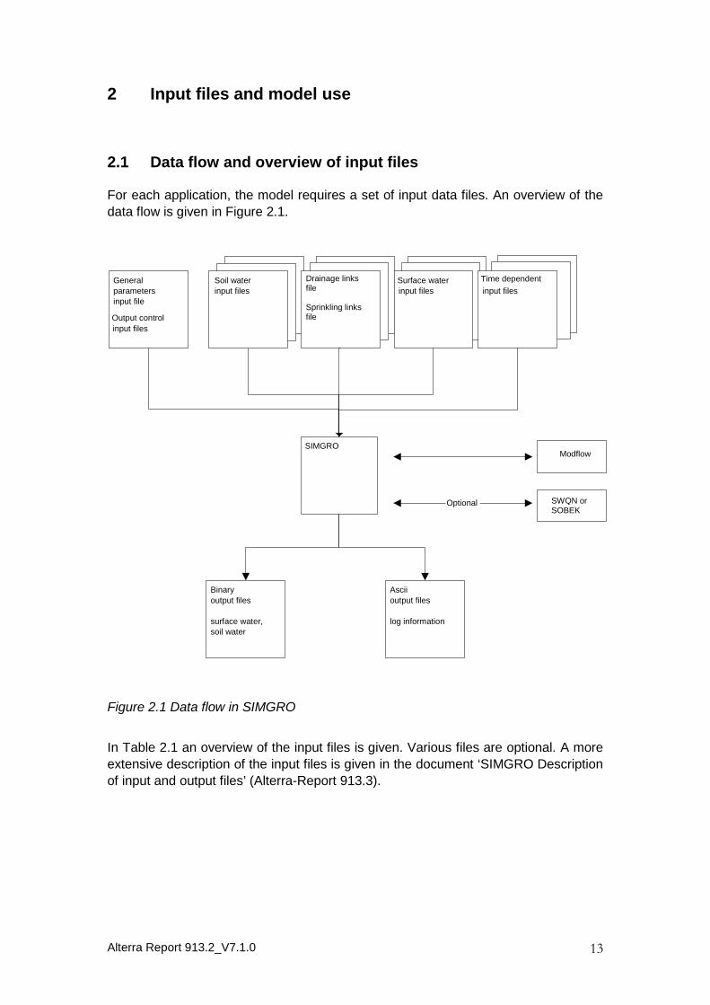
2.1 Data flow and overview of input files
For each application, the model requires a set of input data files. An overview of the
data flow is given in Figure 2.1.
Figure 2.1 Data flow in SIMGRO
In Table 2.1 an overview of the input files is given. Various files are optional. A more
extensive description of the input files is given in the document ‘SIMGRO Description
of input and output files’ (Alterra-Report 913.3).
General
parameters
input file
SIMGRO
Binary
output files
surface water,
soil water
Ascii
output files
log information
input files input files
Surface water
input files
Modflow
SWQN orSOBEK
Optional
Output control
Time dependentSoil water
input files
Drainage linksfile
Sprinkling linksfile
Alterra Report 913.2_V7.1.0 14
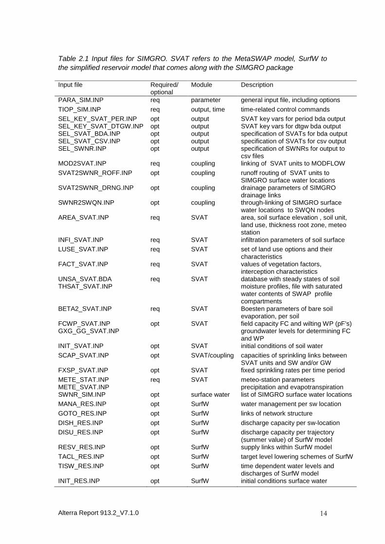
Table 2.1 Input files for SIMGRO. SVAT refers to the MetaSWAP model, SurfW to
the simplified reservoir model that comes along with the SIMGRO package
Input file Required/optional
Module Description
PARA_SIM.INP req parameter general input file, including options
TIOP_SIM.INP req output, time time-related control commands
SEL_KEY_SVAT_PER.INPSEL_KEY_SVAT_DTGW.INP
optopt
outputoutput
SVAT key vars for period bda outputSVAT key vars for dtgw bda output
SEL_SVAT_BDA.INPSEL_SVAT_CSV.INP
optopt
outputoutput
specification of SVATs for bda outputspecification of SVATs for csv output
SEL_SWNR.INP opt output specification of SWNRs for output tocsv files
MOD2SVAT.INP req coupling linking of SVAT units to MODFLOW
SVAT2SWNR_ROFF.INP opt coupling runoff routing of SVAT units toSIMGRO surface water locations
SVAT2SWNR_DRNG.INP opt coupling drainage parameters of SIMGROdrainage links
SWNR2SWQN.INP opt coupling through-linking of SIMGRO surfacewater locations to SWQN nodes
AREA_SVAT.INP req SVAT area, soil surface elevation , soil unit,land use, thickness root zone, meteostation
INFI_SVAT.INP req SVAT infiltration parameters of soil surface
LUSE_SVAT.INP req SVAT set of land use options and theircharacteristics
FACT_SVAT.INP req SVAT values of vegetation factors,interception characteristics
UNSA_SVAT.BDATHSAT_SVAT.INP
req SVAT database with steady states of soilmoisture profiles, file with saturatedwater contents of SWAP profilecompartments
BETA2_SVAT.INP req SVAT Boesten parameters of bare soilevaporation, per soil
FCWP_SVAT.INPGXG_GG_SVAT.INP
opt SVAT field capacity FC and wilting WP (pF’s)groundwater levels for determining FCand WP
INIT_SVAT.INP opt SVAT initial conditions of soil water
SCAP_SVAT.INP opt SVAT/coupling capacities of sprinkling links betweenSVAT units and SW and/or GW
FXSP_SVAT.INP opt SVAT fixed sprinkling rates per time period
METE_STAT.INPMETE_SVAT.INP
req SVAT meteo-station parametersprecipitation and evapotranspiration
SWNR_SIM.INP opt surface water list of SIMGRO surface water locations
MANA_RES.INP opt SurfW water management per sw location
GOTO_RES.INP opt SurfW links of network structure
DISH_RES.INP opt SurfW discharge capacity per sw-location
DISU_RES.INP opt SurfW discharge capacity per trajectory(summer value) of SurfW model
RESV_RES.INP opt SurfW supply links within SurfW model
TACL_RES.INP opt SurfW target level lowering schemes of SurfW
TISW_RES.INP opt SurfW time dependent water levels anddischarges of SurfW model
INIT_RES.INP opt SurfW initial conditions surface water
Alterra Report 913.2_V7.1.0 15
2.2 Setting up the schematization
2.2.1 Coupling in space
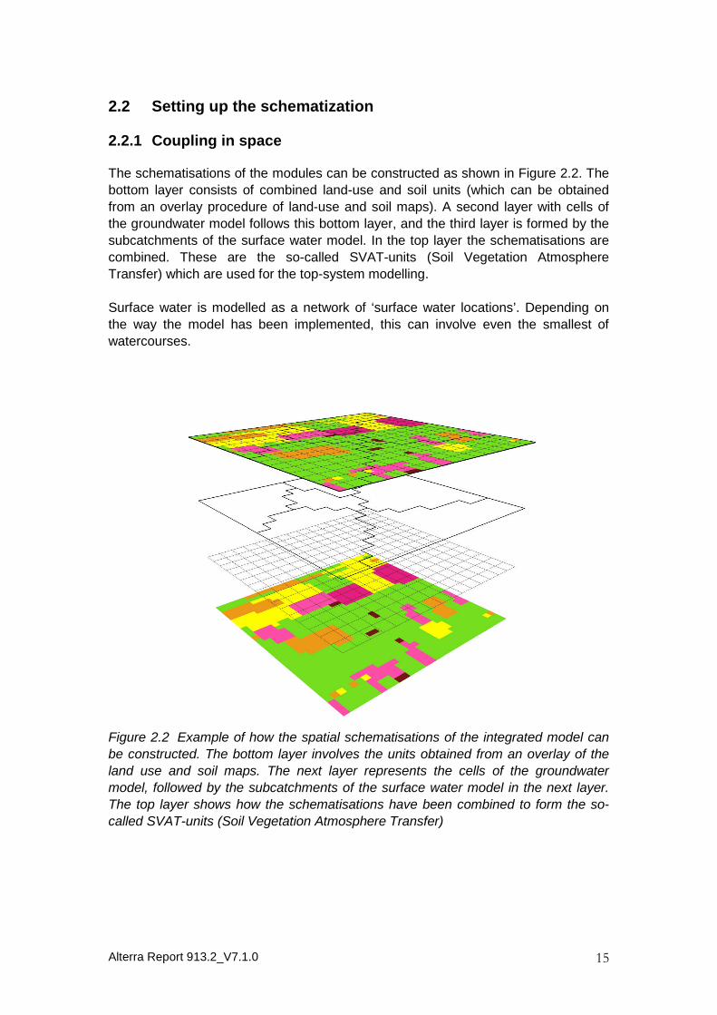
The schematisations of the modules can be constructed as shown in Figure 2.2. The
bottom layer consists of combined land-use and soil units (which can be obtained
from an overlay procedure of land-use and soil maps). A second layer with cells of
the groundwater model follows this bottom layer, and the third layer is formed by the
subcatchments of the surface water model. In the top layer the schematisations are
combined. These are the so-called SVAT-units (Soil Vegetation Atmosphere
Transfer) which are used for the top-system modelling.
Surface water is modelled as a network of ‘surface water locations’. Depending on
the way the model has been implemented, this can involve even the smallest of
watercourses.
Figure 2.2 Example of how the spatial schematisations of the integrated model can
be constructed. The bottom layer involves the units obtained from an overlay of the
land use and soil maps. The next layer represents the cells of the groundwater
model, followed by the subcatchments of the surface water model in the next layer.
The top layer shows how the schematisations have been combined to form the so-
called SVAT-units (Soil Vegetation Atmosphere Transfer)
Alterra Report 913.2_V7.1.0 16
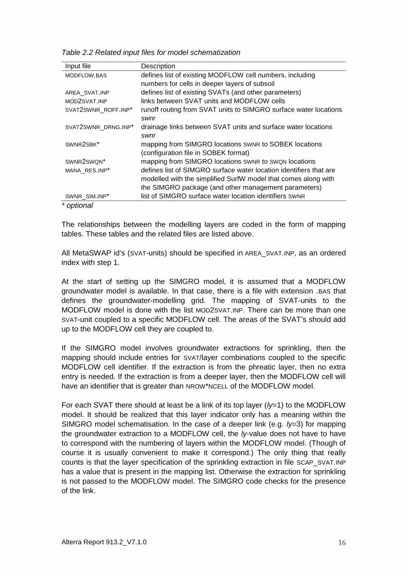
Table 2.2 Related input files for model schematization
Input file Description
MODFLOW.BAS defines list of existing MODFLOW cell numbers, including
numbers for cells in deeper layers of subsoil
AREA_SVAT.INP defines list of existing SVATs (and other parameters)
MOD2SVAT.INP links between SVAT units and MODFLOW cells
SVAT2SWNR_ROFF.INP* runoff routing from SVAT units to SIMGRO surface water locations
swnr
SVAT2SWNR_DRNG.INP* drainage links between SVAT units and surface water locations
swnr
SWNR2SBK* mapping from SIMGRO locations SWNR to SOBEK locations
(configuration file in SOBEK format)
SWNR2SWQN* mapping from SIMGRO locations SWNR to SWQN locations
MANA_RES.INP* defines list of SIMGRO surface water location identifiers that are
modelled with the simplified SurfW model that comes along with
the SIMGRO package (and other management parameters)
SWNR_SIM.INP* list of SIMGRO surface water location identifiers SWNR
* optional
The relationships between the modelling layers are coded in the form of mapping
tables. These tables and the related files are listed above.
All MetaSWAP id’s (SVAT-units) should be specified in AREA_SVAT.INP, as an ordered
index with step 1.
At the start of setting up the SIMGRO model, it is assumed that a MODFLOW
groundwater model is available. In that case, there is a file with extension .BAS that
defines the groundwater-modelling grid. The mapping of SVAT-units to the
MODFLOW model is done with the list MOD2SVAT.INP. There can be more than one
SVAT-unit coupled to a specific MODFLOW cell. The areas of the SVAT’s should add
up to the MODFLOW cell they are coupled to.
If the SIMGRO model involves groundwater extractions for sprinkling, then the
mapping should include entries for SVAT/layer combinations coupled to the specific
MODFLOW cell identifier. If the extraction is from the phreatic layer, then no extra
entry is needed. If the extraction is from a deeper layer, then the MODFLOW cell will
have an identifier that is greater than NROW*NCELL of the MODFLOW model.
For each SVAT there should at least be a link of its top layer (ly=1) to the MODFLOW
model. It should be realized that this layer indicator only has a meaning within the
SIMGRO model schematisation. In the case of a deeper link (e.g. ly=3) for mapping
the groundwater extraction to a MODFLOW cell, the ly-value does not have to have
to correspond with the numbering of layers within the MODFLOW model. (Though of
course it is usually convenient to make it correspond.) The only thing that really
counts is that the layer specification of the sprinkling extraction in file SCAP_SVAT.INP
has a value that is present in the mapping list. Otherwise the extraction for sprinkling
is not passed to the MODFLOW model. The SIMGRO code checks for the presence
of the link.
Alterra Report 913.2_V7.1.0 17
If it is desired to model surface water, the SIMGRO model schematization should
start by defining the SIMGRO surface water locations SWNR. These are listed in
SWNR_SIM.INP. The file can be left out if no surface water simulation is wanted. By
default the model contains a SWNR=0 location.
If a mapping to surface water locations is desired, then these should be given in file
SVAT2SWNR.INP. The used SWNR-references should be present in the list given by
SWNR_SIM.INP. The file does not have to contain records for all of the SVATs that have
been defined in AREA_SVAT.INP. For the SVATs that are not listed the model assumes
a default mapping to SWNR=0. The SVAT2SWNR.INP file can be left out altogether; in
that case the model assumes a mapping of all SVATs to SWNR =0.
The use of the SurfW model for simplified surface water simulation is optional. In that
case the file MANA_RES.INP is present, plus the other SurfW files. The list of SWNR-
identifiers in the first column of MANA_RES.INP defines which of the SIMGRO surface
water locations are modelled by the SurfW model. There can only be one SurfW unit
per SWNR-identifier.
When the SWQN/Surface water model is used for simulating the surface water
dynamics, the file SWNR2SWQN.INP has to be specified. This file relates the identifiers
of the SIMGRO surface water locations to the identifiers of the SWQN model. For
coupling to the SOBEK model the path and name of the so-called configuration file
has to be specified in PARA_SIM.INP. There can be more than one SWNR-identifier
coupled to a specific location of an external surface water model.
For the SVATS’s that are coupled to surface water locations that are not modelled by
SurfW or by SWQN/SOBEK the model model operates in the following manner:
- unrestricted runoff (except for the impediment due to the so-called micro-storage
capacity vxmu, see file AREA_SVAT.INP); no runon;
- drainage and infiltration simulation using the default water levels provided in
SVAT2SWNR_DRNG.INP; if no level is provided in SVAT2SWNR_DRNG.INP and the
surface water location is not coupled, then no infiltration is possible;
- unlimited supply for sprinkling from surface water.
Alterra Report 913.2_V7.1.0 18
2.2.2 Coupling in time
In the file, PARA_SIM.INP the groundwater time step (SIMGRO) should be made equal
to the length of the stress period of MODFLOW. Therefore the bas-file of the
MODFLOW-model should have for the following parameters fixed values:
PERLEN = dtgw (usually 1 d);
NSTP = 1;
TSMULT = 1.
Usually a time step of 1 day is used.
MODFLOW time refers to the length of the time period from the start of the
calculation. SIMGRO uses a time in days (with t =0 at the beginning of a year at
00:00:00) and a Gregorian year. The model user has to be aware of this and has to
synchronise both time indications.

Alterra Report 913.2_V7.1.0 19
2.3 Plant/Soil-Atmosphere interactions
Organization
Table 2.3 Related input files
Input file Description
General
PARA_SIM.INP several general parameters, including the choice of
evapotranspiration model etmdl
METE_STAT.INP meteo-station parameters, for Penman-Monteith method
METE_SVAT.INP meteo-data
LUSE_SVAT.INP sprinkling data, evaporation reduction factors, vegetation type
FACT_SVAT.INP vegetation evapotranspiration factors
VG2CRP_SVAT.INP coupling of vg-index to crops of WOFOST model
SVAT unit-specific
AREA_SVAT.INP land use characteristics, meteorological region number
INFI_SVAT.INP infiltration parameters
SCAP_SVAT.INP sprinkling characteristics
FXSP_SVAT.INP fixed sprinkling demands
2.3.1 Precipitation
Description
For the simulation period, the time series information of the meteorological conditions
should be available in the form of a step-function. This entails that the value of the
time variable is for the start of a new intensity. Especially if a file contains values
per day the novel user can easily misinterpret the given time as the ‘index’ of a
certain day, which can lead to the presumption that the model simulation contains an
errant time shift. The given time values do not necessarily have to contain values for
the beginning of a specific day. In fact, most rainfall data are obtained by gauges that
are read early in the morning, e.g. at 8 AM. In that case the time values should be at
1/3 of a day, i.e. at 0.333, 1.333, and so on.
There can be any number of time steps per day. During the simulation, the meteo-
data will vary per dtsw that is the time step for calculation of the fast processes. For
doing this the model uses time-averaged meteo-values for the dtsw-steps, obtained
by integrating the step functions over time.
The AREA_SVAT file contains a field with the number of the meteorological region. The
model then makes the connection with the number in the file containing the
meteorological data, METE_SVAT.INP. This field can be left blank if use is made of
grids, and so that file METE_SVAT.INP does not need to be present. For input via grids
see the IO-manual Section 2.3.10.
Alterra Report 913.2_V7.1.0 20
Specification
Table 2.4 Input files and related parameters for precipitation
Input file Parameter Unit Description
PARA_SIM.INP dtsw d time step for fast processes
METE_SVAT.INP td d time for start of new value meteo-variable
iy - year number
pr mm precipitation
AREA_SVAT.INP svat - SVAT unit
nmmend - meteorological region number
For using the meteorological data in the top-system modelling, the time step for
the fast processes is used, dtsw (PARA_SIM.INP)
The meteorological data are specified in METE_SVAT.INP. Meteorological data
should be specified from the start to the end of the model run. The data in this file
should be in chronological order. For each time step, the meteo stations should
be in the same order. For each time step, data for all the meteo-stations should
be available.
The time step can be smaller than 1 day. When the user wants to use relatively
short meteo time steps, the groundwater and surface water time steps should be
chosen accordingly (see PARA_SIM.INP).
The meteorological region number specifies the meteorological station. See
METE_SVAT.INP and AREA_SVAT.INP.
2.3.2 Sprinkling
Description
The ‘natural’ precipitation can be augmented by sprinkling. During the growing
season, precipitation deficits are likely to occur regularly. If, in severe cases, the
pressure head in the root zone is lowered beyond the reduction point, crop growth
will be reduced. To avoid this in many parts of the world crops are irrigated.
The SIMGRO sprinkling module contains two steps for the sprinkling simulation:
- determining the demand;
- determining the ‘realization’ by trying to match the demand with the available
supply.
Sprinkling can be triggered by the pressure head in the rootzone or can be
prescribed in a file. When enough supply is available, the demand will be realized as
a sprinkling gift. The source for the sprinkling water has to be specified; it can be
surface water, groundwater or a combination. If sprinkling from both groundwater and
surface water is enabled, sprinkling from surface water has priority. But when in that
case the surface water does not have enough capacity to fulfil the demand the
remainder will be supplied from groundwater.
Sprinkling triggered by pressure head
Automatic sprinkling requirements are specified per land use type in LUSE_SVAT.INP.
For determining the moment to start sprinkling (and to stop) use is made of the
pressure head in the root zone. Sprinkling is triggered when the pressure head in the

Alterra Report 913.2_V7.1.0 21
root zone has fallen below a crop-related ‘start’ value. The user has to specify a
sprinkling gift, gift duration and the length of the rotational period. For instance:
The sprinkling gift equals 25 mm;
The gift duration is 0.5 d;
The rotational period is 10 days;
The pressure head in the rootzone is below the pressure head to begin sprinkling
Then the sprinkling demand equals 50.0 mm d-1 during half a day and a new
demand will not be calculated within 10 days since the start of the sprinkling. Notice
that it concerns a demand. Even if this demand cannot be realised due to the low
availability of water, the model will wait the full length of the rotational period before
checking the sprinkler demand-trigger again.
Prescribed sprinkling demand
For each time a new demand can be specified in the FXSP_SVAT.INP. When the
demand:
is set to value greater than zero, it is interpreted as a fixed sprinkling demand;
is set to zero, it is interpreted as ‘no sprinkling’;
is given a negative value, sprinkling will be calculated depending on the rootzone
pressure head (automatic sprinkling).
We use an example to explain how it works:time year SVAT
unit
sprinkling
demand
(mm d-1
)
0.00 1990 1 0.00
100.00 1990 1 200.00
100.50 1990 1 0.00
150.00 1990 1 -1.00
At time 0.0/1990 a fixed flux of 0.0 mm d-1 is specified for SVAT unit 1; so from this
moment on the automatic sprinkling is switched off. This ‘no sprinkling’ condition lasts
until the next time value (i.e. time 100.0). At time 100.0/1990 a demand is prescribed
of 200 mm d-1 ; it lasts half a day. From then on the demand equals 0.00 mm d-1
again. At time 150.0/1990 the fixed-demand sprinkling is switched off and the
automatic sprinkling is enabled. As this example shows, it is possible to specify the
period of automatic sprinkling for each SVAT unit individually. This then over-rules
the values given LUSE_SVAT.INP.
Demand realization
The demand is read by the model per dtgw-interval, but applied per dtsw-interval.
The demand realization can be less than 100% if one of the following conditions is
limiting:
- the pump capacities given in file SCAP_SVAT.INP;
- the availability of water at the linked surface water locations specified in
SCAP_SVAT.INP;
It is assumed that there always is enough groundwater for sprinkling.
The pump capacities should be set at realistic values, to avoid excessively high
application rates during the the dtsw-intervals, leading to runoff.

Alterra Report 913.2_V7.1.0 22
Sprinkling evaporation
It is well known that quite a relevant part of the sprinkling water evaporates. This can
be specified using the ‘fraction evaporated sprinkling water’ (frevsplu) in
LUSE_SVAT.INP.
Specification
Table 2.5 Input files and related parameters for sprinkling
Input file Parameter Unit DescriptionPARA_SIM.INP dtsw d time step for fast processesLUSE_SVAT.INP lu - land use type
pbgsplu m pressure head begin sprinklingfrevsplu - fraction evaporated sprinkling watergisplu mm gift in rotational periodtigisplu d duration giftrpsplu d rotational perioddybgsplu d beginning of sprinkling period, in days from
beginning of year at 00:00:00dyedsplu d end of sprinkling period
SCAP_SVAT.INP svat - SVAT unitfmmxabgw mm d
-1maximum abstraction from groundwater
fmmxabsw mm d-1
maximum abstraction from surface waterfxabgw m
3d
-1maximum abstraction from groundwater
fxabsw m3
d-1
maximum abstraction from surface watersvatab - SVAT unit from which groundwater is
abstractedlyab - layer number for abstractionswnrab - subcatchment from which surface water is
abstractedFXSP_SVAT.INP td d time from beginning of year at 00:00:00
iy - year numbernnex - SVAT unitfxspi mm d
-1intensity sprinkling demand
For sprinkling simulation, the time step for the fast processes is used dtsw
(PARA_SIM.INP).
The trigger for automatic sprinkling is the pressure head pbgsplu in
LUSE_SVAT.INP, which is specified per land use type.
In SCAP_SVAT.INP several characteristics are defined: the layer for groundwater
sprinkling, the abstraction SVAT unit, the watercourse and the maximum
capacities from groundwater and surface water.
If for both surface water and groundwater capacities are specified, sprinkling from
surface water has priority, and is reduced if the supply to the subcatchment (see
MANA_RES.INP for when the water is from the SurfW model) is insufficient. Supply
from groundwater will then compensate the low availability from surface water.
If both fmmxabgw and fxabgw are specified, the abstraction of fxabgw is used (so
when fmmxabgw = 1 and fxabgw not specified the abstraction equals 1 mm/d and
with fxmmabgw = 1 and fxabgw = 0 the abstraction will be zero). The same
applies for surface water.
If a sprinkling demand is prescribed then this demand is used independent of the
state of the unsaturated soil.
Alterra Report 913.2_V7.1.0 23
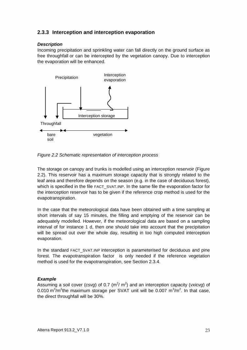
2.3.3 Interception and interception evaporation
Description
Incoming precipitation and sprinkling water can fall directly on the ground surface as
free throughfall or can be intercepted by the vegetation canopy. Due to interception
the evaporation will be enhanced.
Figure 2.2 Schematic representation of interception process
The storage on canopy and trunks is modelled using an interception reservoir (Figure
2.2). This reservoir has a maximum storage capacity that is strongly related to the
leaf area and therefore depends on the season (e.g. in the case of deciduous forest),
which is specified in the file FACT_SVAT.INP. In the same file the evaporation factor for
the interception reservoir has to be given if the reference crop method is used for the
evapotranspiration.
In the case that the meteorological data have been obtained with a time sampling at
short intervals of say 15 minutes, the filling and emptying of the reservoir can be
adequately modelled. However, if the meteorological data are based on a sampling
interval of for instance 1 d, then one should take into account that the precipitation
will be spread out over the whole day, resulting in too high computed interception
evaporation.
In the standard FACT_SVAT.INP interception is parameterised for deciduous and pine
forest. The evapotranspiration factor is only needed if the reference vegetation
method is used for the evapotranspiration, see Section 2.3.4.
Example
Assuming a soil cover (csvg) of 0.7 (m2/ m2) and an interception capacity (vxicvg) of
0.010 m3/m2the maximum storage per SVAT unit will be 0.007 m3/m2. In that case,
the direct throughfall will be 30%.
PrecipitationInterceptionevaporation
Throughfall
Interception storage
baresoil
vegetation
Alterra Report 913.2_V7.1.0 24
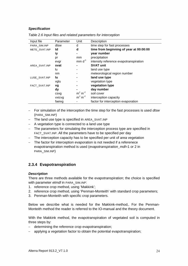
Specification
Table 2.6 Input files and related parameters for interception
Input file Parameter Unit Description
PARA_SIM.INP dtsw d time step for fast processes
METE_SVAT.INP td d time from beginning of year at 00:00:00
iy - year number
pr mm precipitation
evgr mm d-1
intensity reference evapotranspiration
AREA_SVAT.INP svat - SVAT unit
lu - land use type
nm - meteorological region number
LUSE_SVAT.INP lu - land use type
vglu - vegetation type
FACT_SVAT.INP vg - vegetation type
dy - day number
csvg m2
m-2
soil cover
vxicvg m3
m-2
interception capacity
faeivg - factor for interception evaporation
For simulation of the interception the time step for the fast processes is used dtsw
(PARA_SIM.INP)
The land use type is specified in AREA_SVAT.INP
A vegetation type is connected to a land use type
The parameters for simulating the interception process type are specified in
FACT_SVAT.INP. All the parameters have to be specified per day
The interception capacity has to be specified per unit of area vegetation
The factor for interception evaporation is not needed if a referenece
evapotranspiration method is used (evapotranspiration_mdl=1 or 2 in
PARA_SIM.INP)
2.3.4 Evapotranspiration
Description
There are three methods available for the evapotranspiration; the choice is specified
with parameter etmdl in PARA_SIM.INP:
1. reference crop method, using ‘Makkink’;
2. reference crop method, using ‘Penman-Monteith’ with standard crop parameters;
3. Penman-Monteith with specific crop parameters.
Below we describe what is needed for the Makkink-method,. For the Penman-
Monteith method the reader is referred to the IO-manual and the theory document.
With the Makkink method, the evapotranspiration of vegetated soil is computed in
three steps by:
determining the reference crop evapotranspiration;
applying a vegetation factor to obtain the potential evapotranspiration;
Alterra Report 913.2_V7.1.0 25
reducing the potential evapotranspiration to the actual evapotranspiration based
on the soil moisture content.
The implementation of the ‘Feddes’ function for the reduction of evapotranspiration
differs from the implementation used in SWAP. In the implementation of the Feddes
function in SIMGRO, the pressure head values for the reduction of ET due to wet
conditions apply to the pressure head at the soil surface, not in the root zone itself.
In effect, the reduction is based on the groundwater level, which determines the
pressure head at the soil surface under wet conditions. The computed reduction
factor is applied to the root extraction in the whole root zone. To disable the
reduction function for rice, for instance, values of p1 and p2 should be used that are
higher than the maximum inundation depth in a paddy.
For calculating the reduction due to dry conditions, the model first downscales the
pressure head in the root zone to separate values for equal fractions (‘slices’) of it.
The reduction function is then applied to the separate fractions, and then averaged
for the root zone as a whole.
Typically, for agricultural crops, the factors are only available for the growing season.
When the factors are used in the model, the assumption is made that the factors
have been calibrated based on field experiments, involving the total
evapotranspiration, including that of bare soil. Therefore the value of the soil cover is
taken to be 1.0 in the part of the year for which a vegetation factor is available, and
0.0 for the remaining part. So for the vegetated part of the year no separate
calculation for bare soil evaporation is made.
For natural vegetations (and for agricultural grassland) it is assumed that a
vegetation factor is available all the year round.
Evaporation from bare soil will be calculated for the days that the soil cover is less
than 1.0.
For forests the interception evaporation is of great importance. Therefore, one should
preferably not use “all-inclusive” vegetation factors (i.e. inclusive interception).
Urban areas are partly vegetated and partly paved. Simulating urban area should be
done by using separate SVAT’s for the vegetated and the paved parts. The built-up
area should be given a zero or small infiltration capacity (AREA_SVAT.INP) and a small
micro storage capacity from which water can evaporate. It is important to use (near)
zero crop factors, to simulate realistic (near) zero evaporation.
The vegetated part in built-up area is simulated using standard crop factors (for
instance grass).
Alterra Report 913.2_V7.1.0 26
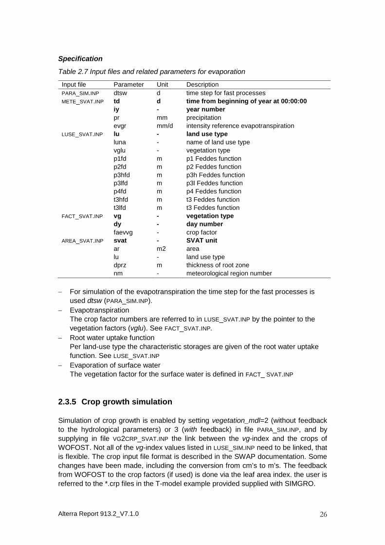
Specification
Table 2.7 Input files and related parameters for evaporation
Input file Parameter Unit Description
PARA_SIM.INP dtsw d time step for fast processes
METE_SVAT.INP td d time from beginning of year at 00:00:00
iy - year number
pr mm precipitation
evgr mm/d intensity reference evapotranspiration
LUSE_SVAT.INP lu - land use type
luna - name of land use type
vglu - vegetation type
p1fd m p1 Feddes function
p2fd m p2 Feddes function
p3hfd m p3h Feddes function
p3lfd m p3l Feddes function
p4fd m p4 Feddes function
t3hfd m t3 Feddes function
t3lfd m t3 Feddes function
FACT_SVAT.INP vg - vegetation type
dy - day number
faevvg - crop factor
AREA_SVAT.INP svat - SVAT unit
ar m2 area
lu - land use type
dprz m thickness of root zone
nm - meteorological region number
For simulation of the evapotranspiration the time step for the fast processes is
used dtsw (PARA_SIM.INP).
Evapotranspiration
The crop factor numbers are referred to in LUSE_SVAT.INP by the pointer to the
vegetation factors (vglu). See FACT_SVAT.INP.
Root water uptake function
Per land-use type the characteristic storages are given of the root water uptake
function. See LUSE_SVAT.INP
Evaporation of surface water
The vegetation factor for the surface water is defined in FACT_ SVAT.INP
2.3.5 Crop growth simulation
Simulation of crop growth is enabled by setting vegetation_mdl=2 (without feedback
to the hydrological parameters) or 3 (with feedback) in file PARA_SIM.INP, and by
supplying in file VG2CRP_SVAT.INP the link between the vg-index and the crops of
WOFOST. Not all of the vg-index values listed in LUSE_SIM.INP need to be linked, that
is flexible. The crop input file format is described in the SWAP documentation. Some
changes have been made, including the conversion from cm’s to m’s. The feedback
from WOFOST to the crop factors (if used) is done via the leaf area index. the user is
referred to the *.crp files in the T-model example provided supplied with SIMGRO.
Alterra Report 913.2_V7.1.0 27
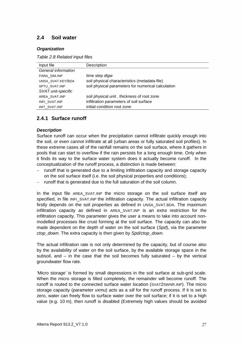
2.4 Soil water
Organization
Table 2.8 Related input files
Input file Description
General information
PARA_SIM.INP time step dtgw
UNSA_SVAT.KEY/BDA soil physical characteristics (metadata-file)
SPTU_SVAT.INP soil physical parameters for numerical calculation
SVAT unit-specific
AREA_SVAT.INP soil physical unit , thickness of root zone
INFI_SVAT.INP infiltration parameters of soil surface
INIT_SVAT.INP initial condition root zone
2.4.1 Surface runoff
Description
Surface runoff can occur when the precipitation cannot infiltrate quickly enough into
the soil, or even cannot infiltrate at all (urban areas or fully saturated soil profiles). In
these extreme cases all of the rainfall remains on the soil surface, where it gathers in
pools that can start to overflow if the rain persists for a long enough time. Only when
it finds its way to the surface water system does it actually become runoff. In the
conceptualization of the runoff process, a distinction is made between:
runoff that is generated due to a limiting infiltration capacity and storage capacity
on the soil surface itself (i.e. the soil physical properties and conditions);
runoff that is generated due to the full saturation of the soil column.
In the input file AREA_SVAT.INP the micro storage on the soil surface itself are
specified, in file INFI_SVAT.INP the infiltration capacity. The actual infiltration capacity
firstly depends on the soil properties as defined in UNSA_SVAT.BDA. The maximum
infiltration capacity as defined in AREA_SVAT.INP is an extra restriction for the
infiltration capacity. This parameter gives the user a means to take into account non-
modelled processes like crust forming at the soil surface. The capacity can also be
made dependent on the depth of water on the soil surface (Spd), via the parameter
ctop_down. The extra capacity is then given by Spd/ctop_down.
The actual infiltration rate is not only determined by the capacity, but of course also
by the availability of water on the soil surface, by the available storage space in the
subsoil, and – in the case that the soil becomes fully saturated – by the vertical
groundwater flow rate.
‘Micro storage’ is formed by small depressions in the soil surface at sub-grid scale.
When the micro storage is filled completely, the remainder will become runoff. The
runoff is routed to the connected surface water location (SVAT2SWNR.INP). The micro
storage capacity (parameter vxmu) acts as a sill for the runoff process. If it is set to
zero, water can freely flow to surface water over the soil surface; if it is set to a high
value (e.g. 10 m), then runoff is disabled (Extremely high values should be avoided
Alterra Report 913.2_V7.1.0 28
because they cause extra memory use for the building of storage tables.). If a certain
SVAT is not coupled to any surface water unit (like is the case when only the
MetaSWAP module of SIMGRO is used in combination with MODFLOW), then the
surface water level is set to -9999. and thus does not obstruct the runoff process in
any manner. If the runoff is modelled in MODFLOW itself, then the MetaSWAP runoff
should be disabled.
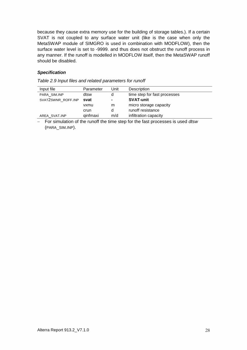
Specification
Table 2.9 Input files and related parameters for runoff
Input file Parameter Unit Description
PARA_SIM.INP dtsw d time step for fast processes
SVAT2SWNR_ROFF.INP svat - SVAT-unit
vxmu m micro storage capacity
crun d runoff resistance
AREA_SVAT.INP qinfmaxi m/d infiltration capacity
For simulation of the runoff the time step for the fast processes is used dtsw
(PARA_SIM.INP).
Alterra Report 913.2_V7.1.0 29
2.4.2 Unsaturated flow
Description
For each SVAT-unit a soil physical unit has to be specified (see AREA_SVAT.INP). This
soil physical unit is a standard soil type with specific characteristics specified in
UNSA_SVAT.BDA. This file contains the meta-data for the storage and flux
characteristics. The data for these standard types are assembled using the model
SWAP (Wesseling, 1991). A ready-to-use database is available for the standard soil
types of the Netherlands. For other soil types a standard procedure is available using
Van Genuchten parameters for a steady-state version of the SWAP model
(Groenendijk, 2006).
Root zone depths are specified per SVAT-unit and are assumed not to vary in time.
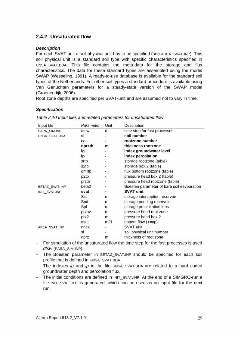
Specification
Table 2.10 Input files and related parameters for unsaturated flow
Input file Parameter Unit Description
PARA_SIM.INP dtsw d time step for fast processes
UNSA_SVAT.BDA sl - soil number
rz - rootzone number
dprztb m thickness rootzone
ig - index groundwater level
ip - index percolation
srtb - storage rootzone (table)
s2tb - storage box 2 (table)
qmrtb - flux bottom rootzone (table)
p2tb - pressure head box 2 (table)
prztb - pressure head rootzone (table)
BETA2_SVAT.INP beta2 - Boesten parameter of bare soil eavporation
INIT_SVAT.INP svat - SVAT unit
Sic m storage interception reservoir
Spd m storage ponding reservoir
Spl m storage precipitation lens
przav m pressure head root zone
prz2 m pressure head box 2
qsat m/d bottom flow (+=up)
AREA_SVAT.INP nnex - SVAT unit
sl - soil physical unit number
dprz m thickness of root zone
For simulation of the unsaturated flow the time step for the fast processes is used
dtsw (PARA_SIM.INP).
The Boesten parameter in BETA2_SVAT.INP should be specified for each soil
profile that is defined in UNSA_SVAT.BDA.
The indexes ig and ip in the file UNSA_SVAT.BDA are related to a hard coded
groundwater depth and percolation flux.
The initial conditions are defined in INIT_SVAT.INP. At the end of a SIMGRO-run a
file INIT_SVAT.OUT is generated, which can be used as an input file for the next
run.

Alterra Report 913.2_V7.1.0 30
Alterra Report 913.2_V7.1.0 31
2.5 Drainage
Description
Drainage can be simulated in two ways:
- Using standard MODFLOW functionalities (drainage and river records)
This is described in detail in the MODFLOW documentation;
- Using the SIMGRO functionality (using the file SVAT2SWNR_DRNG.INP)
In this case, the fluxes are connected to watercourses for which a water balance
is calculated.
The SIMGRO drainage option can be used in combination with any of the options for
surface water simulation, including the hydraulic models.
The assignment of the drainage fluxes is specified in the file SVAT2SWNR_DRNG.INP.
Note that not all of the drainage fluxes from a certain SVAT unit have to be assigned
to the same location that is specified in SVAT2SWNR.INP: in SVAT2SWNR_DRNG.INP the
assignment of a drainage record to a surface water location is specified explicitly,
and thus can deviate from that in SVAT2SWNR.INP. The assignment to a watercourse
not only determines where the water goes to, but also the water level that is used in
the drainage flux calculation itself.
The dimensions of the watercourses and drainage systems (from
SVAT2SWNR_DRNG.INP) are used to calculate the volume-stage relationships, which
are used for the surface water simulations. The dimensions are also used for the
calculations of drainage fluxes. The surface water location to which the drainage
device is connected to is also specified in SVAT2SWNR_DRNG.INP.
It is also possible to use the MODFLOW packages (DRN/RIV/GLS). But in that case
the fluxes are not anymore coupled to the SIMGRO surface water locations. This
does not have to be a problem if the drainage involves interaction with a large canal
that is anyhow not modelled within the scope of SIMGRO package.
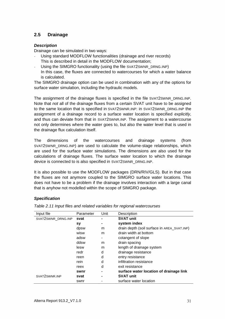
Specification
Table 2.11 Input files and related variables for regional watercourses
Input file Parameter Unit Description
SVAT2SWNR_DRNG.INP svat - SVAT unit
sy - system index
dpsw m drain depth (soil surface in AREA_SVAT.INP)
wisw m drain width at bottom
adsw - cotangent of slope
ddsw m drain spacing
lesw m length of drainage system
redr d drainage resistance
reen d entry resistance
rein d infiltration resistance
reex d exit resistance
swnr - surface water location of drainage link
SVAT2SWNR.INP svat - SVAT unit
swnr - surface water location

Alterra Report 913.2_V7.1.0 33
2.6 Surface water
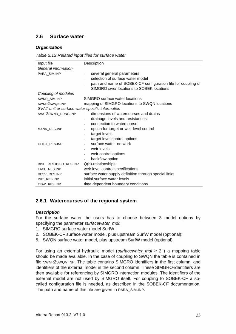
Organization
Table 2.12 Related input files for surface water
Input file Description
General information
PARA_SIM.INP - several general parameters
- selection of surface water model
- path and name of SOBEK-CF configuration file for coupling of
SIMGRO swnr locations to SOBEK locations
Coupling of modules
SWNR_SIM.INP SIMGRO surface water locations
SWNR2SWQN.INP mapping of SIMGRO locations to SWQN locations
SVAT unit or surface water specific information
SVAT2SWNR_DRNG.INP - dimensions of watercourses and drains
- drainage levels and resistances
- connection to watercourse
MANA_RES.INP - option for target or weir level control
- target levels
- target level control options
GOTO_RES.INP - surface water network
- weir levels
- weir control options
- backflow option
DISH_RES /DISU_RES.INP Q(h)-relationships
TACL_RES.INP weir level control specifications
RESV_RES.INP surface water supply definition through special links
INIT_RES.INP initial surface water levels
TISW_RES.INP time dependent boundary conditions
2.6.1 Watercourses of the regional system
Description
For the surface water the users has to choose between 3 model options by
specifying the parameter surfacewater_mdl:
1. SIMGRO surface water model SurfW;
2. SOBEK-CF surface water model, plus upstream SurfW model (optional);
5. SWQN surface water model, plus upstream SurfW model (optional);
For using an external hydraulic model (surfacewater_mdl ≥ 2 ) a mapping table
should be made available. In the case of coupling to SWQN the table is contained in
file SWNR2SWQN.INP. The table contains SIMGRO-identifiers in the first column, and
identifiers of the external model in the second column. These SIMGRO-identifiers are
then available for referencing by SIMGRO interaction modules. The identifiers of the
external model are not used by SIMGRO itself. For coupling to SOBEK-CF a so-
called configuration file is needed, as described in the SOBEK-CF documentation.
The path and name of this file are given in PARA_SIM.INP.
Alterra Report 913.2_V7.1.0 34
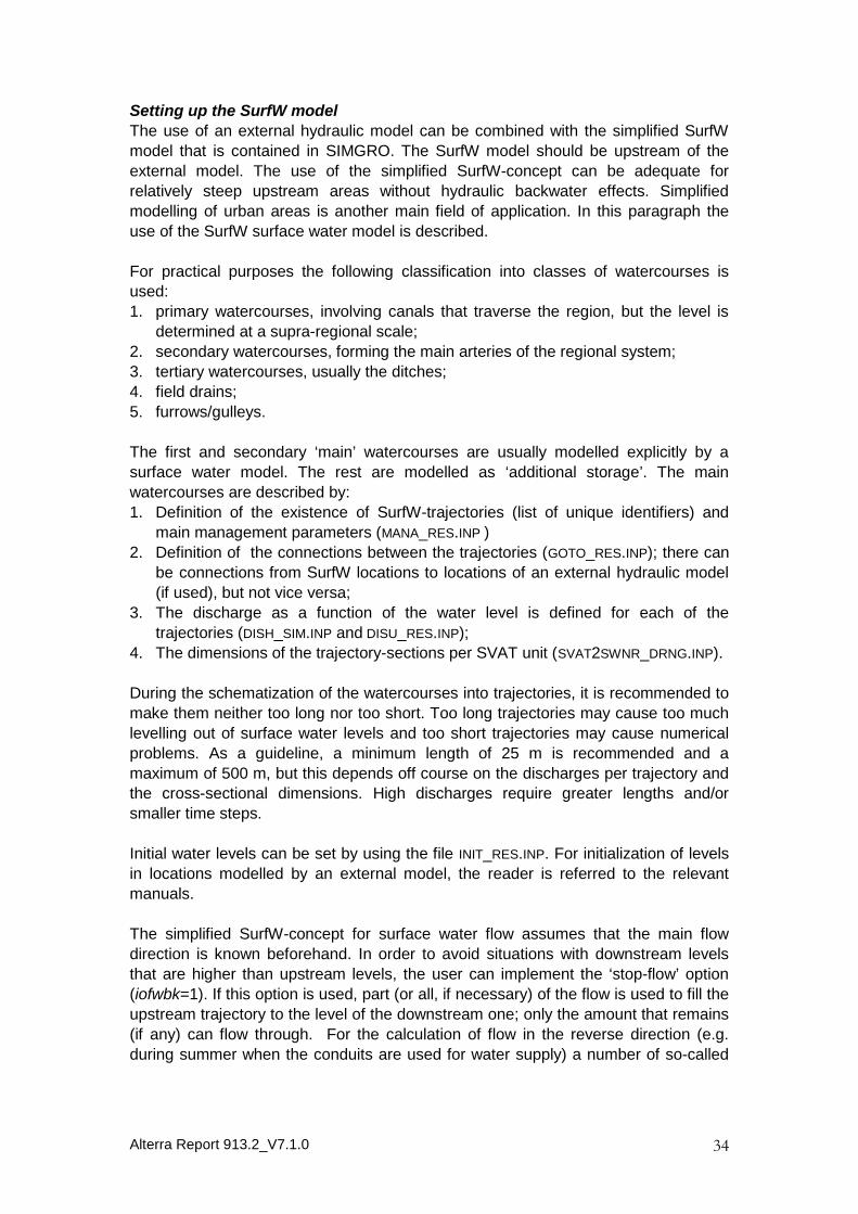
Setting up the SurfW model
The use of an external hydraulic model can be combined with the simplified SurfW
model that is contained in SIMGRO. The SurfW model should be upstream of the
external model. The use of the simplified SurfW-concept can be adequate for
relatively steep upstream areas without hydraulic backwater effects. Simplified
modelling of urban areas is another main field of application. In this paragraph the
use of the SurfW surface water model is described.
For practical purposes the following classification into classes of watercourses is
used:
1. primary watercourses, involving canals that traverse the region, but the level is
determined at a supra-regional scale;
2. secondary watercourses, forming the main arteries of the regional system;
3. tertiary watercourses, usually the ditches;
4. field drains;
5. furrows/gulleys.
The first and secondary ‘main’ watercourses are usually modelled explicitly by a
surface water model. The rest are modelled as ‘additional storage’. The main
watercourses are described by:
1. Definition of the existence of SurfW-trajectories (list of unique identifiers) and
main management parameters (MANA_RES.INP )
2. Definition of the connections between the trajectories (GOTO_RES.INP); there can
be connections from SurfW locations to locations of an external hydraulic model
(if used), but not vice versa;
3. The discharge as a function of the water level is defined for each of the
trajectories (DISH_SIM.INP and DISU_RES.INP);
4. The dimensions of the trajectory-sections per SVAT unit (SVAT2SWNR_DRNG.INP).
During the schematization of the watercourses into trajectories, it is recommended to
make them neither too long nor too short. Too long trajectories may cause too much
levelling out of surface water levels and too short trajectories may cause numerical
problems. As a guideline, a minimum length of 25 m is recommended and a
maximum of 500 m, but this depends off course on the discharges per trajectory and
the cross-sectional dimensions. High discharges require greater lengths and/or
smaller time steps.
Initial water levels can be set by using the file INIT_RES.INP. For initialization of levels
in locations modelled by an external model, the reader is referred to the relevant
manuals.
The simplified SurfW-concept for surface water flow assumes that the main flow
direction is known beforehand. In order to avoid situations with downstream levels
that are higher than upstream levels, the user can implement the ‘stop-flow’ option
(iofwbk=1). If this option is used, part (or all, if necessary) of the flow is used to fill the
upstream trajectory to the level of the downstream one; only the amount that remains
(if any) can flow through. For the calculation of flow in the reverse direction (e.g.
during summer when the conduits are used for water supply) a number of so-called
Alterra Report 913.2_V7.1.0 35
‘backflow’ options are available (iofwbk=2,3 and 4). The backflow option has to be
specified per watercourse in the file GOTO_RES.INP.
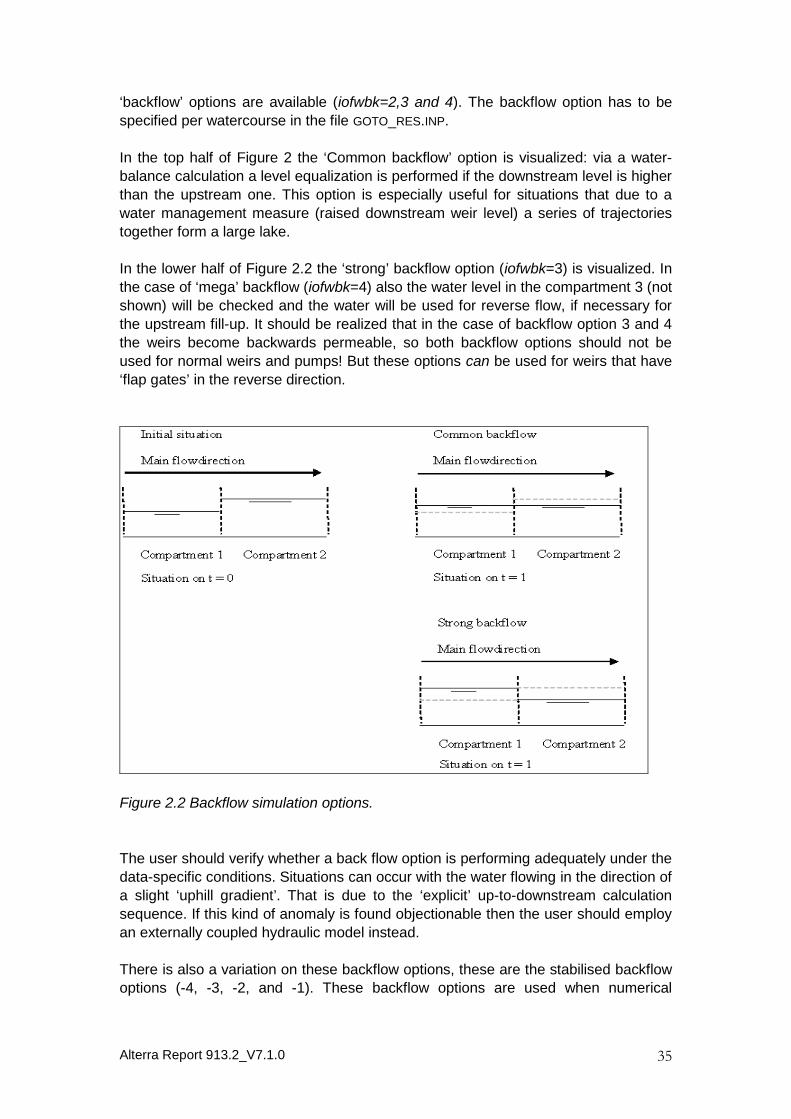
In the top half of Figure 2 the ‘Common backflow’ option is visualized: via a water-
balance calculation a level equalization is performed if the downstream level is higher
than the upstream one. This option is especially useful for situations that due to a
water management measure (raised downstream weir level) a series of trajectories
together form a large lake.
In the lower half of Figure 2.2 the ‘strong’ backflow option (iofwbk=3) is visualized. In
the case of ‘mega’ backflow (iofwbk=4) also the water level in the compartment 3 (not
shown) will be checked and the water will be used for reverse flow, if necessary for
the upstream fill-up. It should be realized that in the case of backflow option 3 and 4
the weirs become backwards permeable, so both backflow options should not be
used for normal weirs and pumps! But these options can be used for weirs that have
‘flap gates’ in the reverse direction.
Figure 2.2 Backflow simulation options.
The user should verify whether a back flow option is performing adequately under the
data-specific conditions. Situations can occur with the water flowing in the direction of
a slight ‘uphill gradient’. That is due to the ‘explicit’ up-to-downstream calculation
sequence. If this kind of anomaly is found objectionable then the user should employ
an externally coupled hydraulic model instead.
There is also a variation on these backflow options, these are the stabilised backflow
options (-4, -3, -2, and -1). These backflow options are used when numerical
Alterra Report 913.2_V7.1.0 36
stabilisation of the calculations is needed. The negative backflow options can be
used when the calculations in a certain compartment are not stable. The minus sign
causes the algorithm to ‘wait one time step’ before rising from below the threshold of
the Q(h)-relationship (in the case of a weir that is the crest) to above it. This option
was devised for suppressing the premature spilling of water over a weir crest just
downstream of a bifurcation.
There are several other ways of stabilizing the surface water calculations. The first is
to reduce the time step dtsw. A second option is to change the parameter dhmxsw.
This parameter defines the maximum allowed change in surface water level over
dtsw. If the model wants to exceed this change, then some of the inflow is
temporarily ‘parked’; it is subsequently added to the flow during the next time step.
Using the recommended values of 0.20 m for dhmxsw and 1 hr for dtsw, the water
level can (theoretically) change by 24*0.2 = 4.80 m/d. That is enough to
accommodate any realistic fluctuations for medium sized water courses.

Alterra Report 913.2_V7.1.0 37
Specification
Table 2.13 Input files and related variables for setting up the SurfW model
Input file Parameter Unit Description
PARA_SIM.INP tdbgsm d time of transition from “winter” to
“summer”, in days from beginning of year
at 00:00:00
tdedsm d time of transition from summer to winter
dtgw d time step for slow processes
dtsw d time step for fast processes
dhmxsw - maximum change in surface water level
over dtsw
SVAT2SWNR_DRNG.INP svat - SVAT unit
sy - system index
dpsw m drain depth
wisw m drain width at bottom
adsw - cotangent of slope
ddsw m drain spacing
lesw m length of drainage system
swnr - surface water location of drainage link
GOTO_RES.INP swnr - number water course
swnrgo - watercourse water is conducted to
lvwrsm m+MSL summer weir level (ioma = 2 or 4)
lvwrwt m+MSL winter weir level (ioma = 1 or 2)
lvwrlw m+MSL lowest possible weir level
iofwbk - option for backflow
glnr m+MSL soil surface elevation next to weir
lvcv m+MSL elevation of culvert
alfa m(3-beta)
/s coefficient of discharge relationship
beta - exponent of discharge relationship
MANA_RES.INP swnr - surface water location
ioma - option for weir/target in summer/winter
lvtasm m+MSL summer target level (ioma = 1 or 3)
lvtawt m+MSL winter target level (ioma = 3 or 4)
DISH_RES.INP or swnr - surface water location
DISU_RES.INP dhwr m energy head above weir crest
fmwr l/s/ha discharge capacity of weir
fswr m3/s discharge capacity of weir
swnrgo - “goto” sw location
TISW_RES.INP td d time from beginning of year at
00:00:00
iy - year
nrex - surface water location
hhwrnw see iolv new weir/target level
flswnw m3/d new surface water inflow rate
swrgo - goto subcatchment in case of a new
weir/target level
INIT_RES.INP nrex - surface water location
hhsw m initial surface water level
fliw m3 surface water inflow
flow m3 surface water outflow
Vmpa m3 temporarily stored volume (stabilisation)

Alterra Report 913.2_V7.1.0 38
Table 2.14 General values for numerical approximation
Name General value Unit Description
dhmxsw 0.20 m Maximum change in sw-level per dtsw
Summer or winter period
This period is specified in PARA_SIM.INP. The period between idbgsm and idedsm
is the summer period, which has the following characteristics:
o the summer weir or target levels are valid;
o the dynamic water level control for the summer is active (when specified),
see GOTO_RES.INP and MANA_RES.INP;
The winter period has the following characteristics:
o the winter weir or target levels are valid;
o the dynamic water level control for the winter is active (when specified),
see GOTO_RES.INP and MANA_RES.INP
Time step for surface water module
In PARA_SIM.INP the time step for the surface water module, dtsw, is specified.
The time steps for groundwater and surface water calculations usually have a
value of respectively 0.25 and 0.05 days. Of course, this depends on the goal of
the study and the system modelled. In highly dynamic systems, it is advisable to
reduce the time step for surface water to for instance 0.01 day;
Parameters for numerical approximationThe parameter dhmxsw has to be specified in PARA_SIM.INP. Usually standardvalues are used.In Table 2.15 the general value for dhmxsw is given.
Surface water structure
The surface water structure is defined in GOTO_RES.INP. In the surface water
structure, no closed loops are allowed; but supply via closed loops can be
specified via RESV_RES.INP (see Section 2.6.3);
The file includes the specification of optional Q-∆h relationships, which are used
for water retention simulations (see IO-manual)
Q(h)-relationships
See DISH_RES.INP and DISU_RES.INP.
It is not allowed to decrease the discharge capacity of a weir with increasing
energy head above the weir crest.
DISU_RES.INP specifies the Q(h)-relationship for summer situations.
Upstream flow
The default backflow (iofwbk) option is set in PARA_SIM.INP. The backflow option
can be specified per watercourse in the file GOTO_RES.INP. The latter will overrule
the default value.
Initial surface water conditions
The initial conditions are defined in INIT_RES.INP.
At the end of a SIMGRO-run a file INIT_RES.OUT is generated, which can be used
as an input file for the next run (after renaming).
Boundary conditions
Time dependent weir levels and inflow fluxes can be chosen as a boundary
condition (TISW_RES.INP).
Dimensions of the watercourses
See SVAT2SWNR_DRNG.INP.

Alterra Report 913.2_V7.1.0 39
2.6.2 Weirs and pumps
Description
When weirs are implemented in the model, not only the weir levels or target level
should be assigned (GOTO_RES.INP and MANA_RES.INP), but also the relationship
between water level and discharge should be specified (DISH_SIM.INP).
Water level control with a weir can be done either indirectly by manipulating the weir
crest or directly by manipulating the target water level.
When in the model definition the target level is activated, the model itself will
calculate the optimal weir crest. The weir crest will in that case be adjusted in such a
way that the water level upstream equals the target level (if there is enough water for
that). The weir crest cannot, however, become lower than the lowest possible weir
level (as defined in GOTO_RES.INP)!
The SIMGRO-code also has the possibility of letting the weir/target levels be
determined by groundwater level (or surface water level or soil water content). In that
case a water level control scheme must be specified in the form of a table, with per
record:
a groundwater level in the monitoring SVAT unit i;
a lowering of the target/weir level in trajectory n.
The records must form a consistent set, with decreasing groundwater level (starting
from 0 at the soil surface) and decreasing lowering of the target/weir level. The
principle being ‘the higher the groundwater level, the lower the weir/target level
should be’, in order to counteract the negative effects of too wet conditions. The
model interpolates to get the corresponding lowering of the weir or target level. If the
current groundwater level is deeper than the deepest groundwater level in the table,
the lowering for the deepest groundwater level is taken.
Alterra Report 913.2_V7.1.0 40
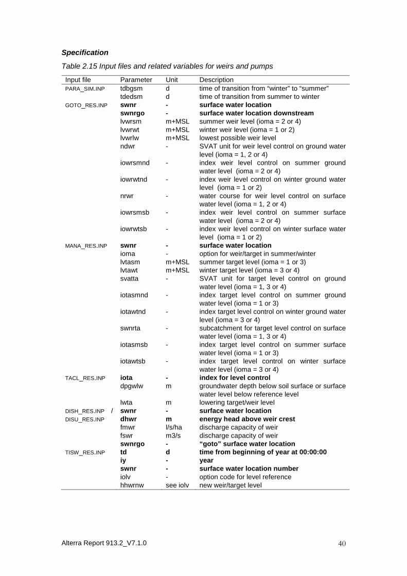
Specification
Table 2.15 Input files and related variables for weirs and pumps
Input file Parameter Unit Description
PARA_SIM.INP tdbgsm d time of transition from “winter” to “summer”tdedsm d time of transition from summer to winter
GOTO_RES.INP swnr - surface water locationswnrgo - surface water location downstreamlvwrsm m+MSL summer weir level (ioma = 2 or 4)lvwrwt m+MSL winter weir level (ioma = 1 or 2)lvwrlw m+MSL lowest possible weir levelndwr - SVAT unit for weir level control on ground water
level (ioma = 1, 2 or 4)iowrsmnd - index weir level control on summer ground
water level (ioma = 2 or 4)iowrwtnd - index weir level control on winter ground water
level (ioma = 1 or 2)nrwr - water course for weir level control on surface
water level (ioma = 1, 2 or 4)iowrsmsb - index weir level control on summer surface
water level (ioma = 2 or 4)iowrwtsb - index weir level control on winter surface water
level (ioma = 1 or 2)MANA_RES.INP swnr - surface water location
ioma - option for weir/target in summer/winterlvtasm m+MSL summer target level (ioma = 1 or 3)lvtawt m+MSL winter target level (ioma = 3 or 4)svatta - SVAT unit for target level control on ground
water level (ioma = 1, 3 or 4)iotasmnd - index target level control on summer ground
water level (ioma = 1 or 3)iotawtnd - index target level control on winter ground water
level (ioma = 3 or 4)swnrta - subcatchment for target level control on surface
water level (ioma = 1, 3 or 4)iotasmsb - index target level control on summer surface
water level (ioma = 1 or 3)iotawtsb - index target level control on winter surface
water level (ioma = 3 or 4)TACL_RES.INP iota - index for level control
dpgwlw m groundwater depth below soil surface or surfacewater level below reference level
lwta m lowering target/weir levelDISH_RES.INP /DISU_RES.INP
swnr - surface water locationdhwr m energy head above weir crestfmwr l/s/ha discharge capacity of weirfswr m3/s discharge capacity of weirswnrgo - “goto” surface water location
TISW_RES.INP td d time from beginning of year at 00:00:00iy - yearswnr - surface water location numberiolv - option code for level referencehhwrnw see iolv new weir/target level
Alterra Report 913.2_V7.1.0 41
Summer or winter period
This period is specified in PARA_SIM.INP. The period between idbgsm and idedsm
is the summer period, which has the following characteristics:
o The summer weir or target levels are valid;
o The dynamic water level control for the summer is active (when specified),
see GOTO_RES.INP and MANA_RES.INP;
The winter period has the following characteristics:
o The winter weir or target levels are valid;
o The dynamic water level control for the winter is active (when specified),
see GOTO_RES.INP and MANA_RES.INP
Target levels and weir levels (summer and winter)
Both target and weir levels can be specified. MANA_RES.INP specifies the target
levels and GOTO_RES.INP the weir levels. The parameter ioma in MANA_RES.INP
determines the use of target or weir level in the model.
Weir and target levels can be specified as time dependent levels, see
TISW_RES.INP.
Q(h)-relationships
See DISH_RES.INP and DISU_RES.INP.
It is not allowed to decrease the discharge capacity of a weir with increasing
energy head above the weir crest.
DISU_RES.INP specifies the Q(h)-relationship for summer situations.
Dynamic target or weir level control on surface water levels, groundwater levels.
The control on root zone saturation is not implemented.
See MANA_RES.INP and GOTO_RES.INP in combination with TACL_RES.INP
The indexes iowrsmnd, iowrwtnd, iowrsmsb, iowrwtsb, iowrsmfr, iowrwtfr refer to
the indexes in the file TACL_RES.INP.
When because of the implementation of more control levels several target levels
are calculated, the lowest target level will be used.
2.6.3 Surface water supply
Description
During summer, many regions receive surface water supply. The reason for
supplying the water can be diverse. In the higher parts of the Netherlands, the reason
is usually to supply water for sprinkling and sub-irrigation. In the lower parts (which
are below sea level), the supply is mainly used for maintaining water quality at an
acceptable level. In the SurfW model, there are two ways of implementing water
supply:
1. ‘out of nowhere’, from outside the model region;
2. through special links that involve the transfer from one location to the next.
Per location with water supply, only one type of water source can be used.
Supply from outside the model region
The supply is specified in the file MANA_SIM.INP using the parameters fxsuswsb for
the supply capacity and dptasu for defining the water level drop that triggers the
actual supply. The latter takes place when the water level in a location drops below
the weir/target level by more than dptasu.
Alterra Report 913.2_V7.1.0 42
m
n
kQI
QE
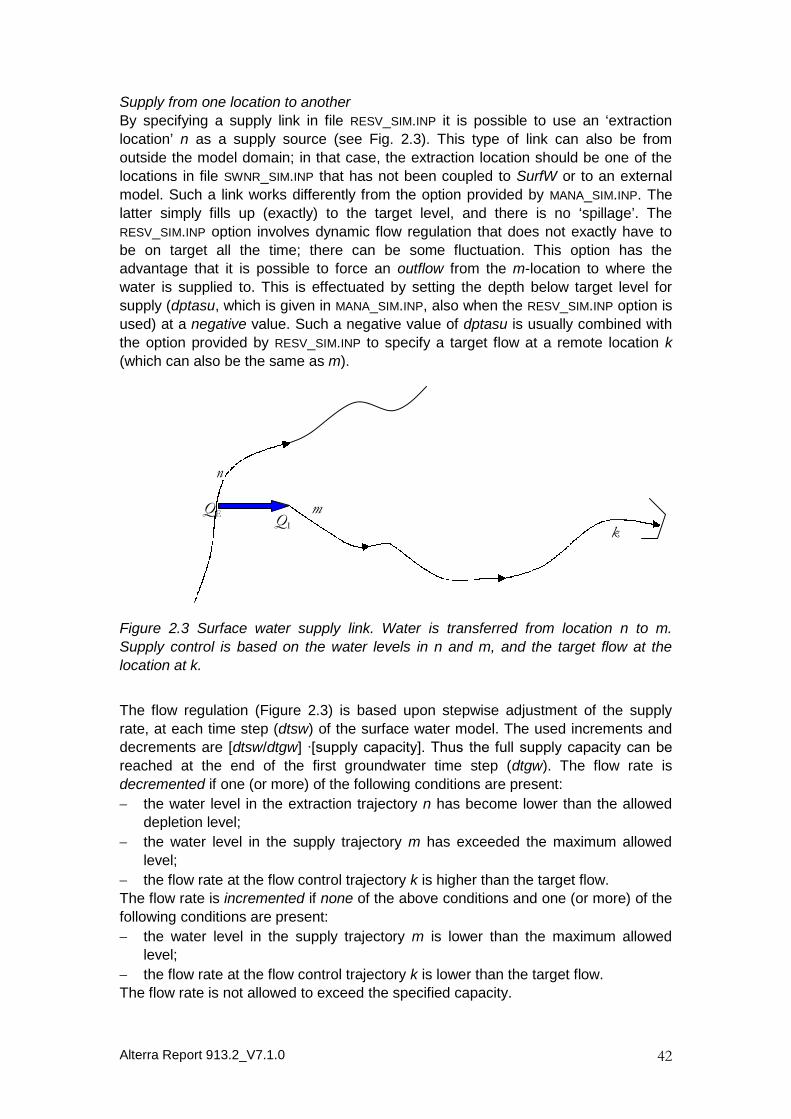
Supply from one location to another
By specifying a supply link in file RESV_SIM.INP it is possible to use an ‘extraction
location’ n as a supply source (see Fig. 2.3). This type of link can also be from
outside the model domain; in that case, the extraction location should be one of the
locations in file SWNR_SIM.INP that has not been coupled to SurfW or to an external
model. Such a link works differently from the option provided by MANA_SIM.INP. The
latter simply fills up (exactly) to the target level, and there is no ‘spillage’. The
RESV_SIM.INP option involves dynamic flow regulation that does not exactly have to
be on target all the time; there can be some fluctuation. This option has the
advantage that it is possible to force an outflow from the m-location to where the
water is supplied to. This is effectuated by setting the depth below target level for
supply (dptasu, which is given in MANA_SIM.INP, also when the RESV_SIM.INP option is
used) at a negative value. Such a negative value of dptasu is usually combined with
the option provided by RESV_SIM.INP to specify a target flow at a remote location k
(which can also be the same as m).
Figure 2.3 Surface water supply link. Water is transferred from location n to m.
Supply control is based on the water levels in n and m, and the target flow at the
location at k.
The flow regulation (Figure 2.3) is based upon stepwise adjustment of the supply
rate, at each time step (dtsw) of the surface water model. The used increments and
decrements are [dtsw/dtgw] ∙[supply capacity]. Thus the full supply capacity can be
reached at the end of the first groundwater time step (dtgw). The flow rate is
decremented if one (or more) of the following conditions are present:
the water level in the extraction trajectory n has become lower than the allowed
depletion level;
the water level in the supply trajectory m has exceeded the maximum allowed
level;
the flow rate at the flow control trajectory k is higher than the target flow.
The flow rate is incremented if none of the above conditions and one (or more) of the
following conditions are present:
the water level in the supply trajectory m is lower than the maximum allowed
level;
the flow rate at the flow control trajectory k is lower than the target flow.
The flow rate is not allowed to exceed the specified capacity.
Alterra Report 913.2_V7.1.0 43
It is possible to use a single extraction location for supplying multiple locations.
However, the model cannot handle supply to one target trajectory from different
extraction locations. Neither can this form of supply be combined with the supply
option of MANA_RES.INP.
The criterium for the depletion level of the extraction trajectory is purely based on the
available water in storage at the beginning of the time step. Therefore, the algorithm
does not take into account that there can be inflow to the extraction trajectory from
e.g. an upstream trajectory. The amount of water that can be supplied in this manner
is limited by the storage characteristics, the weir/target level and the allowed level of
depletion in the extraction trajectory. This storage-related amount can be supplied at
each time step of the surface water. So the realized supply flow rate can be
increased by either increasing the storage capacity or by making the time step
smaller.
Because the supply capacity is used for determining the flow increment/decrement, it
is important to specify a realistic value; otherwise the flow regulation will cause
undesired spillage situations.
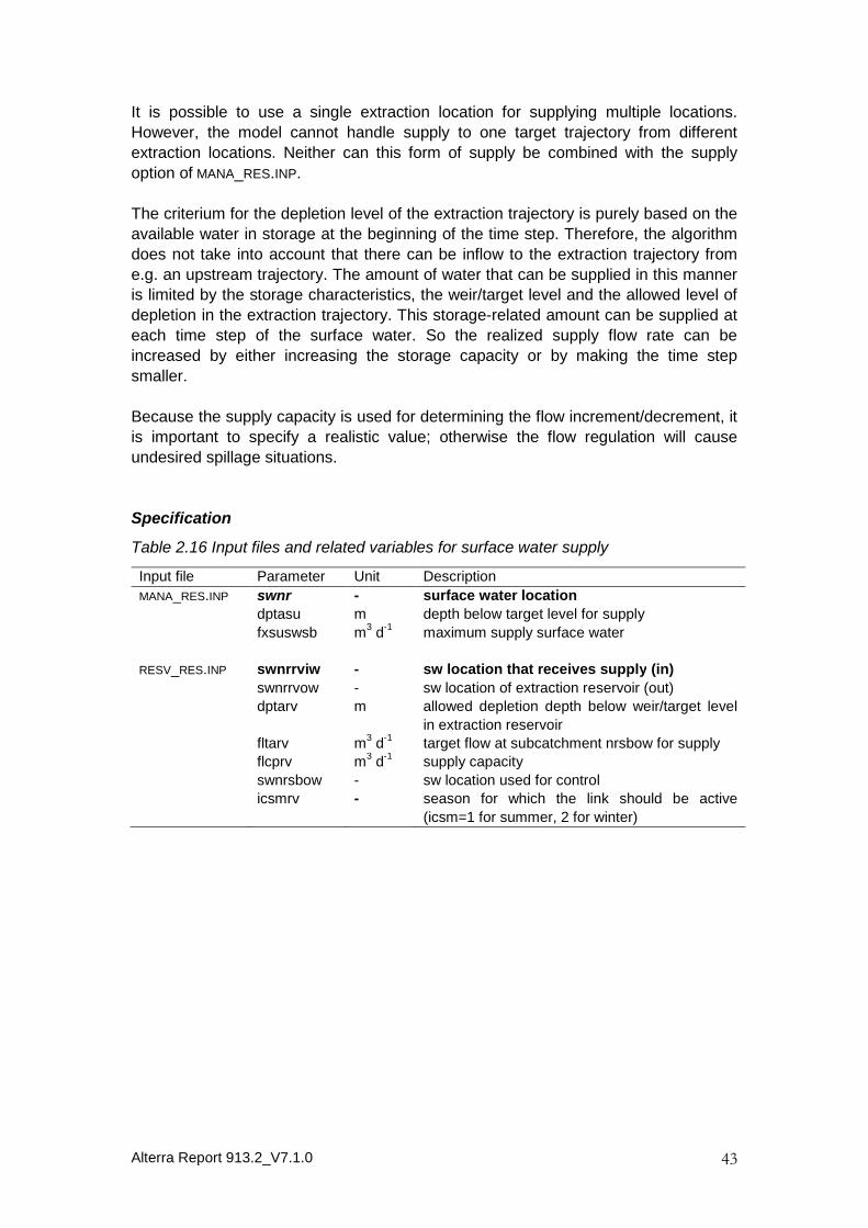
Specification
Table 2.16 Input files and related variables for surface water supply
Input file Parameter Unit Description
MANA_RES.INP swnr - surface water location
dptasu m depth below target level for supply
fxsuswsb m3
d-1
maximum supply surface water
RESV_RES.INP swnrrviw - sw location that receives supply (in)
swnrrvow - sw location of extraction reservoir (out)
dptarv m allowed depletion depth below weir/target level
in extraction reservoir
fltarv m3
d-1
target flow at subcatchment nrsbow for supply
flcprv m3
d-1
supply capacity
swnrsbow - sw location used for control
icsmrv - season for which the link should be active
(icsm=1 for summer, 2 for winter)

Alterra Report 913.2_V7.1.0 44
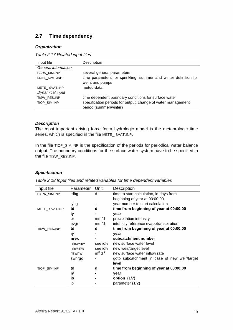
Alterra Report 913.2_V7.1.0 45
2.7 Time dependency
Organization
Table 2.17 Related input files
Input file Description
General information
PARA_SIM.INP several general parameters
LUSE_SVAT.INP time parameters for sprinkling, summer and winter definition for
weirs and pumps
METE_ SVAT.INP meteo-data
Dynamical input
TISW_RES.INP time dependent boundary conditions for surface water
TIOP_SIM.INP specification periods for output, change of water management
period (summer/winter)
Description
The most important driving force for a hydrologic model is the meteorologic time
series, which is specified in the file METE_ SVAT.INP.
In the file TIOP_SIM.INP is the specification of the periods for periodical water balance
output. The boundary conditions for the surface water system have to be specified in
the file TISW_RES.INP.
Specification
Table 2.18 Input files and related variables for time dependent variables
Input file Parameter Unit DescriptionPARA_SIM.INP tdbg d time to start calculation, in days from
beginning of year at 00:00:00
iybg - year number to start calculation
METE_ SVAT.INP td d time from beginning of year at 00:00:00
iy - year
pr mm/d precipitation intensity
evgr mm/d intensity reference evapotranspiration
TISW_RES.INP td d time from beginning of year at 00:00:00
iy - year
nrex - subcatchment number
hhswnw see iolv new surface water level
hhwrnw see iolv new weir/target level
flswnw m3
d-1
new surface water inflow rate
swnrgo - goto subcatchment in case of new weir/target
level
TIOP_SIM.INP td d time from beginning of year at 00:00:00
iy - year
io - option (1/7)
ip - parameter (1/2)

Alterra Report 913.2_V7.1.0 46
Simulation period
The length of the simulation run is controlled by MODFLOW using information
from the bas file. The start time is needed in PARA_SIM.INP in order to know where
to start with the reading of the meteorological data, and to know when to switch to
summer/winter regimes.
Meteo-data
The meteorologic data are specified in METE_ SVAT.INP. Meteorologic data should
be specified from the time to start the model run until the time to stop. The data in
this file should be in chronological order.
The time step can also be smaller than 1 day. When the user wants to use
relatively short meteo time steps, the appropriate groundwater and surface water
time step (see PARA_SIM.INP) should be used
Surface water levels, weir levels, inflow flux
Time dependent weir levels and inflow flux boundaries can be chosen.
See file TISW_RES.INP
Change of water management period, using io=1 in TIOP_SIM.INP. The change of
season is ‘ forced’ by setting the option parameter to ip=1 for change to summer,
2 for change to winter. This overrules the parameters idbgsm and idedsm that are
given in PARA_SIM.INP. Once a specification of io=1 has been given, the season
will only change through a subsequent season specification.
Periods for output, using io=7 in TIOP_SIM.INP
This triggers the writing to periodical water balance output files (*_PER.*)
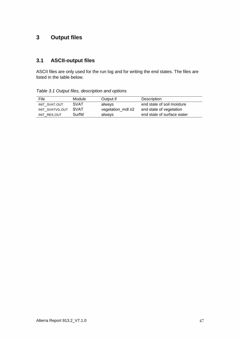
Alterra Report 913.2_V7.1.0 47
3 Output files
3.1 ASCII-output files
ASCII files are only used for the run log and for writing the end states. The files are
listed in the table below.
Table 3.1 Output files, description and options
File Module Output if Description
INIT_SVAT.OUT SVAT always end state of soil moisture
INIT_SVATVG.OUT SVAT vegetation_mdl ≥2 end state of vegetation
INIT_RES.OUT SurfW always end state of surface water
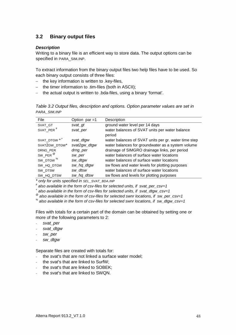
Alterra Report 913.2_V7.1.0 48
3.2 Binary output files
Description
Writing to a binary file is an efficient way to store data. The output options can be
specified in PARA_SIM.INP.
To extract information from the binary output files two help files have to be used. So
each binary output consists of three files:
the key information is written to .key-files,
the timer information to .tim-files (both in ASCII);
the actual output is written to .bda-files, using a binary ‘format’.
Table 3.2 Output files, description and options. Option parameter values are set in
PARA_SIM.INP
File Option par =1 Description
SVAT_GT svat_gt ground water level per 14 days
SVAT_PER# svat_per water balances of SVAT units per water balance
period
SVAT_DTGW *,+ svat_dtgw water balances of SVAT units per gr. water time step
SVAT2GW_DTGW* svat2gw_dtgw water balances for groundwater as a system volume
DRNG_PER drng_per drainage of SIMGRO drainage links, per period
SW_PER@ sw_per water balances of surface water locations
SW_DTGW% sw_dtgw water balances of surface water locations
SW_HQ_DTGW sw_hq_dtgw sw flows and water levels for plotting purposes
SW_DTSW sw_dtsw water balances of surface water locations
SW_HQ_DTSW sw_hq_dtsw sw flows and levels for plotting purposes
* only for units specified in SEL_SVAT_BDA.INP#
also available in the form of csv-files for selected units, if svat_per_csv=1+
also available in the form of csv-files for selected units, if svat_dtgw_csv=1@
also available in the form of csv-files for selected swnr locations, if sw_per_csv=1%
also available in the form of csv-files for selected swnr locations, if sw_dtgw_csv=1
Files with totals for a certain part of the domain can be obtained by setting one or
more of the following parameters to 2:
- svat_per
- svat_dtgw
- sw_per
- sw_dtgw
Separate files are created with totals for:
- the svat’s that are not linked a surface water model;
- the svat’s that are linked to SurfW;
- the svat’s that are linked to SOBEK;
- the svat’s that are linked to SWQN.
Alterra Report 913.2_V7.1.0 49
3.3 Extracting data from binary files
Several post-processing programs have been developed to read the binary output
and to convert it to the desired format. The binary files have the extension ‘bda’,
which stands for binary direct access. Each of the binary files is accompanied by a ‘.
key’ file containing information about the content of the database, and a ‘. tim’ file
containing information about the simulation times for which data are available.
Unfortunately, binary files produced by Fortran do not have a standardized format.
Thus it is crucial that the used postprocessing programs have been compiled with the
same compiler version as the used version of MODFLOW-SIMGRO! For that
reason the names of all executables include the used compiler version.
Determining statistics of the phreatic regime
The programme bda2gt.exe generates a text file with the mean lowest, the mean
highest, the spring and the mean groundwater level (in Dutch abbreviated to GLG,
GHG, GVG and GG). These statistics of the groundwater levels are calculated for all
the SVAT units. The groundwater levels should be available at bimonthly intervals
(i.e. the levels on the 14th and 28th day of the month) for a period of at least two
years. The files are obtained by setting svat_gt=1 in PARA_SIM.INP. The data are
written to the pair of database-files files svat_gt.key and svat_gt.bda. The so-called
key-file svat_gt.key (in ASCII format, thus viewable in a text-editing programme)
defines the content of the binary file svat_gt.bda that contains the actual data. Apart
from the mentioned files the user should have available the file SVAT.asc, which is
an ASCII grid-file of the SVAT-polygons. The polygons should first have been
converted to a grid (using a GIS-system), with the smallest of the SVAT-polygons as
the gridding unit. The gridding should be done for the ‘id’ of the SVAT-units. The grid-
file can be exported with the ‘Export data source’ functonality, using the option ‘ASCII
raster’.
The programme is called with 10 arguments; the command line for using the
programme is:
bda2gt.exe < log-file> <key-file> <item> <gt.csv><SVAT.asc> <glg.asc> <ghg.asc> <gvg.asc> <gg.asc><gt.asc>
All file references should include the full directory path. The columns of the csv-file
represent:
- SVAT unit
- glg, the mean lowest groundwater level
- ghg, the mean highest groundwater level
- gvg, the spring groundwater level
- gg, mean groundwater level
- gt-group1 (new group)
- gt-group2
- gt-group3
The units are transformed from m+MSL to centimetres below soil surface.
The output for glg, ghg, gvg, gg and gt (ranging from 1 to 8) is also written to ASCII-
grid files (integer-format), using SVAT.asc for mapping.
Alterra Report 913.2_V7.1.0 50
Extracting time series
The programme BDA2TIME.EXE can be used for extracting a time series from a binary
file. It has to be called with 4 arguments:
BDA2TIME.EXE <log-file> <key-file> <item> <SVAT/SWNR>
All file references should include the full directory path.
It is not possible to specify more than one SVATunit/SWNR in a single call of
bda2time.
An example of a query for a time series of the groundwater levels in SVAT unit
30433:
bda2time.exe d:\logs\svat.log d:\data\svat_dtgw.key Hgw 30433
The generated text-file is written to the directory location of the key-file and the name
of the csv-file (in ASCII format) is composed as follows:
<item>_<SVAT/SWNR>.csv
The columns of the csv-file represent:
‘yyyy-mm-dd; hr:mn:ss’
value of item, with the length unit as given in the key-file, in m
A ‘model time’ of for instance ‘0.0 1989’ is converted to: '1988-31-12;23:59:59'.
Extracting model area series
The programme BDA2GRID.EXE has to be called with at least 5 arguments. When no
day-year combination is specified, all the periods of the tim-file are selected and the
long-term average of the time series is computed for each spatial unit:
BDA2GRID.EXE <log-file> <key-file> <item> <SVAT.asc> <output.asc>
(<<day> <year>, .. >)n
All file references should include the full directory path. Several day-year
combinations can be specified. Apart from the database files (key-file and bda-file)
the user should have available the file SVAT.asc, which is an ASCII grid-file of the
SVAT-polygons. The polygons should first have been converted to a grid (using a
GIS-system), with the smallest of the SVAT-polygons as the gridding unit. The
gridding should be done for the ‘id’ of the SVAT-units. The grid-file can be exported
with the ‘Export data source’ functonality, using the option ‘ASCII raster’.
For example, for every SVAT unit the mean root zone pressure head for day 273 and
274 of 1996 is obtained with:
BDA2GRID.EXE d:\logs\svat.log d:\data\svat_dtgw.key phrz01d:\tmp\SVAT.asc d:\tmp\phrz01.asc 273.0 1996 274.0 1996.

Alterra Report 913.2_V7.1.0 51
This programme generates a csv-file with the item information for the specified
periods.
The generated text-file is written to the path directory <path> and the name of the
csv-file is composed as follows:
<item>.csv
The columns of the csv-file (in ASCII format) represent:
SVAT unit/subcatchment
value of item, with the length unit in mm
The average for the item over the period(s) is presented in case of flux and storage
terms. In case of levels, the values at the end of the specified periods are averaged.
If the input file SVAT.asc exists, the output is also written to an ASCII-grid file
(floating-format), using SVAT.asc for mapping.

Alterra Report 913.2_V7.1.0 53
4 Programme execution
4.1 Hardware requirements
To run SIMGRO you are advised to use at least the following system configuration:
IBM compatible PC with a pentium processor (≥ 2 GHz);
1 Gb RAM;
CD drive for installation of SIMGRO;
hard disk with at least 10 Gb free;
Windows XP - Windows 7.
Especially if use is made of an external disk via the USB connection, the user should
make sure that it has been formatted under the NTFS system, and not under the
FAT32 system that the disks usually have as the off-the-shelf format. If the format is
left at FAT32, then the output files will not be able to become bigger than about 4 Gb.
4.2 Executables
In the name of the executable the length of the reserved X-array of MODFLOW will
be apparent (e.g. “_LENX250M” = a LENX dimension of 250 million). This is the only
hard-coded array dimension. All SIMGRO arrays are dimensioned dynamically in the
initial phase of programme running. The following information about the specific
programe build is contained in the name of the executable::
the MODFLOW version tag, e.g. “_V16R1_1_1_0”;
the SIMGRO-version number, e.g. V7_0_0;
the SVN-version number of the build, which is the unique key to the version;
whether or not the programme has been compiled with checks of the array
bounds; this is indicated by the code “Release” for no check of bounds and
“Debug” for the version that includes this check (and other ones);
whether or not the code-parallellization has been enabled; the version with
parallellized SIMGRO and MetaSWAP routines is recognizable from the text
string _pll_ in the name of the executable, the sequential version by the string
_seq_ in the name;
the compiler used for the compilation; this information is important because the
used utilities BDA2TIME.EXE and BDA2GRID.EXE should have been generated with
the same compiler (Intel/other), otherwise the reading of the binary output files
can be erroneous.
An example of a programme name is (programme compiled with Intel Fortran 11.1)
“MODFLOW_V16R1_1_1_0-SIMGRO_V7_0_0_SVN150_RELEASE_PLL_IFORT110.EXE”.
We strongly recommend that with each major change of input data the user first
makes a short run with “Debug” version, to check whether array bounds are being
violated. Such violations can occur due to user-errors in data files.

Alterra Report 913.2_V7.1.0 54
4.3 MODFLOW-SIMGRO solution scheme parameters
The MODFLOW-SIMGRO solution scheme follows the standard MODFLOW patternof:- an outer loop for setting of head-sensitive parameters, like the phreatic storage
coefficient;- an inner loop for solving the the set of equations for the groundwater model.
The iteration scheme for the convergence between MetaSWAP and MODFLOW
would continue indefinitely if not some sort of smoothing operation is performed
between the outer-loop iterations; the latter are indexed by the variable iter. The
iteration would never stop because – especially in a large model – there will always
be a situation where the saturated flux is very sensitive to the specified storage
coefficient of the phreatic layer. In order to use the computational resources
efficiently we use the following smoothing scheme:
sc1(iter) = sc1new, for iter ≤ iterur1
sc1(iter) = sc1new * ω + sc1(iter - 1)*(1- ω), for iterur1+1 ≤ iter ≤ iterur2-1
sc1(iter) = sc1(iter - 1) for iterur2 ≤ iter
where sc1new is the new storage coefficient based on the latest information from
MODFLOW and MetaSWAP, and ω is the under-relaxation factor defined as:
ω =1.0 - (iter - iterur1))/(iterur2 - iterur1)
The parameters iterur1 and iterur2 are specified in file PARA_SIM.INP. The default
values are respectively 5 and 7.
The MODFLOW file with extension “pcg” contains the parameters that control theMODFLOW part of the scheme. We recommend the following settings, with thenames of variables as used in the MODFLOW2005 manual:- MXITER=iterur2+2, for the maximum number of outer-loop iterations;- ITER1=20, for the maximum number of inner-loop iterations;- NPCOND=1;- HCLOSE=0.005 m, for the stopping criterium of the head change;- RCLOSE=1000.- RELAX=0.98- NBPOL, IPRPCG, DAMP = 0
During execution the programme sends information about the convergence between
MODFLOW and MetaSWAP to the screen, and also to file INFO_SIM.OUT. The
maximum deviation (+ and -) is reported. A maximum deviation of a few decimeters
often occurs. That does not necessaraily harm the accuracy of the model, because
no water balance errors are made. The error made is simply that the MODFLOW
fluxes are not computed with the same head as that of MetaSWAP; the latter is
always consistent with the saturated flux of MODFLOW. The user should evaluate
the accuracy of the model for the goal of the application. Often it will suffice to
compare the long-term statistics of the groundwater regime, as computed from the
MetaSWAP levels and the MODFLOW ones. For convenience of the user the output
file SVAT_GT.BDA contains information about the levels in both models.
Alterra Report 913.2_V7.1.0 55
4.4 Problems during execution
A user may encounter problems during execution of the model. To determine the
cause of these problems the following steps should be taken:
check the amount of free memory (RAM), paging file, and hard disk space;
run the “Debug” version of the executable if that has not been done recently;
inspect the reported errors in the files INFO_TIM.OUT, INFO_SIM.OUT and
INFO_SVAT.OUT. Open these files, read the (last) lines in the file and try to
determine if there is a mistake in the input file. The log-files are:
o INFO_SIM.OUT: This file contains the SIMGRO-log of running MODFLOW-
SIMGRO.EXE. It is recommended to always consult this file. Several checks
will be done while reading the input-files. Warnings and errors are written.
These warnings will not cause the programme to stop, but can be of help
in preventing wrong input.
o INFO_SVAT.OUT: This files contains the error messages of the soil moisture
module.
check if there are tabs in the input files or check the positions in the input file.
Check if there are empty lines at the end of your input file.
It is important to check that SIMGRO has ended due to the end-call of MODFLOW,
and not due to a crash. The latter can for instance happen if the file with
meteorological data does not continue to the next day after the end time of the run.

Alterra Report 913.2_V7.1.0 57
Literature
Van Walsum, P.E.V., A.A. Veldhuizen, P.J.T. van Bakel, F.J.E. van der Bolt, P.E.
Dik, P. Groenendijk, E.P. Querner, M.F.R. Smit, 2010. SIMGRO 7.0; Description of
theory and model implementation. Wageningen, Alterra, Alterra-rapport 913.1.
Van Walsum, P.E.V, 2010. SIMGRO Input and output reference manual..
Wageningen, Alterra, Alterra-rapport 913.3.

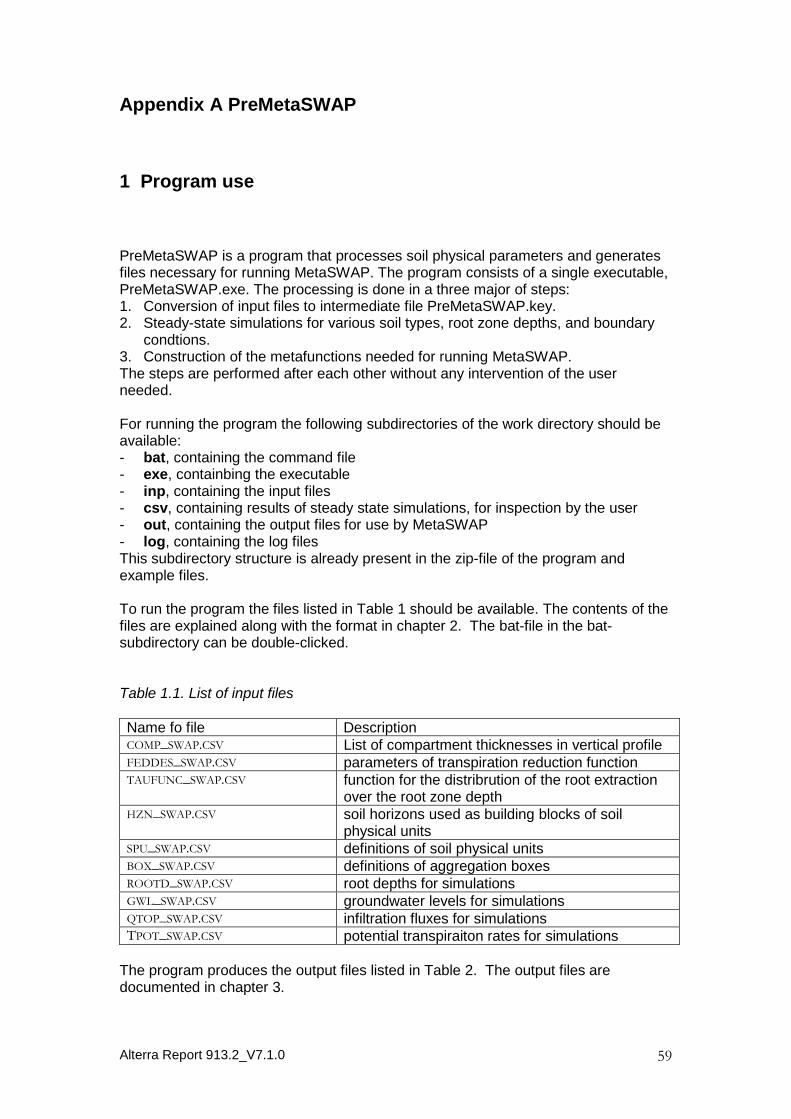
Alterra Report 913.2_V7.1.0 59
Appendix A PreMetaSWAP
1 Program use
PreMetaSWAP is a program that processes soil physical parameters and generatesfiles necessary for running MetaSWAP. The program consists of a single executable,PreMetaSWAP.exe. The processing is done in a three major of steps:1. Conversion of input files to intermediate file PreMetaSWAP.key.2. Steady-state simulations for various soil types, root zone depths, and boundary
condtions.3. Construction of the metafunctions needed for running MetaSWAP.The steps are performed after each other without any intervention of the userneeded.
For running the program the following subdirectories of the work directory should beavailable:- bat, containing the command file- exe, containbing the executable- inp, containing the input files- csv, containing results of steady state simulations, for inspection by the user- out, containing the output files for use by MetaSWAP- log, containing the log filesThis subdirectory structure is already present in the zip-file of the program andexample files.
To run the program the files listed in Table 1 should be available. The contents of thefiles are explained along with the format in chapter 2. The bat-file in the bat-subdirectory can be double-clicked.
Table 1.1. List of input files
Name fo file DescriptionCOMP_SWAP.CSV List of compartment thicknesses in vertical profileFEDDES_SWAP.CSV parameters of transpiration reduction functionTAUFUNC_SWAP.CSV function for the distribrution of the root extraction
over the root zone depthHZN_SWAP.CSV soil horizons used as building blocks of soil
physical unitsSPU_SWAP.CSV definitions of soil physical unitsBOX_SWAP.CSV definitions of aggregation boxesROOTD_SWAP.CSV root depths for simulationsGWL_SWAP.CSV groundwater levels for simulationsQTOP_SWAP.CSV infiltration fluxes for simulationsTPOT_SWAP.CSV potential transpiraiton rates for simulations
The program produces the output files listed in Table 2. The output files aredocumented in chapter 3.
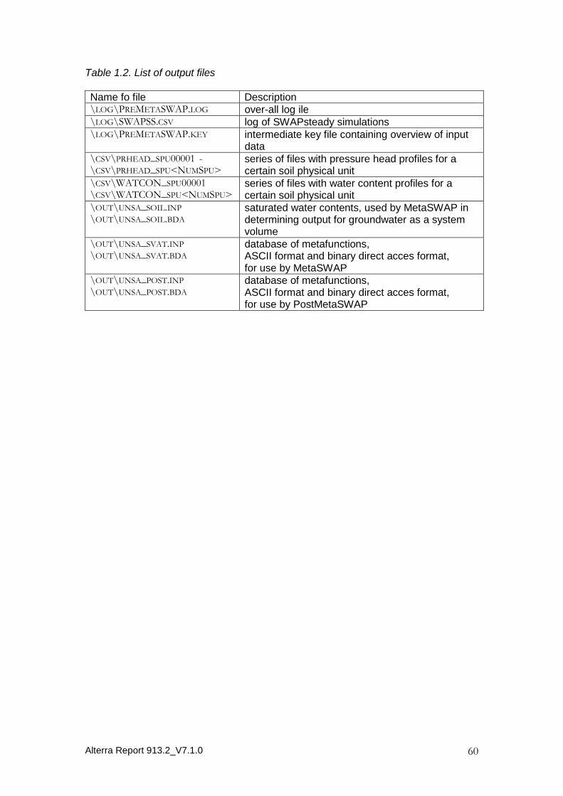
Alterra Report 913.2_V7.1.0 60
Table 1.2. List of output files
Name fo file Description\LOG\PREMETASWAP.LOG over-all log ile\LOG\SWAPSS.CSV log of SWAPsteady simulations\LOG\PREMETASWAP.KEY intermediate key file containing overview of input
data\CSV\PRHEAD_SPU00001 -\CSV\PRHEAD_SPU<NUMSPU>
series of files with pressure head profiles for acertain soil physical unit
\CSV\WATCON_SPU00001\CSV\WATCON_SPU<NUMSPU>
series of files with water content profiles for acertain soil physical unit
\OUT\UNSA_SOIL.INP
\OUT\UNSA_SOIL.BDA
saturated water contents, used by MetaSWAP indetermining output for groundwater as a systemvolume
\OUT\UNSA_SVAT.INP
\OUT\UNSA_SVAT.BDA
database of metafunctions,ASCII format and binary direct acces format,for use by MetaSWAP
\OUT\UNSA_POST.INP
\OUT\UNSA_POST.BDA
database of metafunctions,ASCII format and binary direct acces format,for use by PostMetaSWAP

Alterra Report 913.2_V7.1.0 61
2 Input file descriptions
The specification for the input file descriptions is tabulated below. In the subsequentsections the files are described and in all cases examples are included. If necessary,descriptions are clarified through additional remarks.
Table 2.1 Input item characteristics
Item DescriptionName name of the parameter or variableFormat input formatUnit unit of the input parameter or variableDescription brief description of the parameter or variableMin. minimum value allowedMax. maximum value allowed

Alterra Report 913.2_V7.1.0 62
2.1 COMP_SWAP.CSV
Variable format and descriptionname Format unit descriptioncp I - compartment indexthickns F m thickness of compartment
Variable characteristicsname min maxcp 1 -thickns 0.010 10.00
Examplecp thickns1 0.0102 0.0103 0.0104 0.0105 0.0106 0.0257 0.0258 0.0259 0.025... ...
RemarksThe sum of the compartment thicknesses should be exactly equal to 100 m. (Forother depths of the profile please consult Alterra). Any number of compartments canbe used.
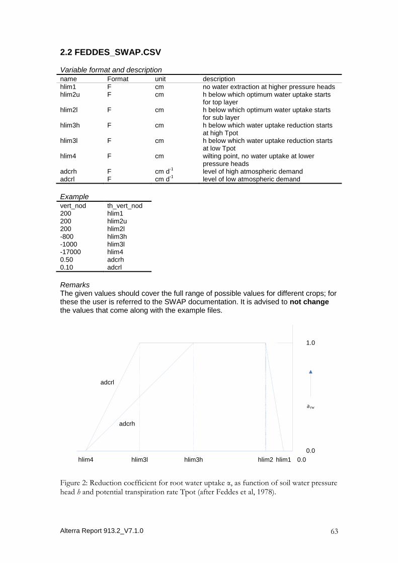
Alterra Report 913.2_V7.1.0 63
2.2 FEDDES_SWAP.CSV
Variable format and descriptionname Format unit descriptionhlim1 F cm no water extraction at higher pressure headshlim2u F cm h below which optimum water uptake starts
for top layerhlim2l F cm h below which optimum water uptake starts
for sub layerhlim3h F cm h below which water uptake reduction starts
at high Tpothlim3l F cm h below which water uptake reduction starts
at low Tpothlim4 F cm wilting point, no water uptake at lower
pressure headsadcrh F cm d
-1level of high atmospheric demand
adcrl F cm d-1
level of low atmospheric demand
Examplevert_nod th_vert_nod200 hlim1200 hlim2u200 hlim2l-800 hlim3h-1000 hlim3l-17000 hlim40.50 adcrh0.10 adcrl
RemarksThe given values should cover the full range of possible values for different crops; forthese the user is referred to the SWAP documentation. It is advised to not changethe values that come along with the example files.
Figure 2: Reduction coefficient for root water uptake α, as function of soil water pressure head h and potential transpiration rate Tpot (after Feddes et al, 1978).
hlim4 hlim3l hlim3h hlim2 hlim1
1.0
0.0
0.0
a rw
adcrh
adcrl
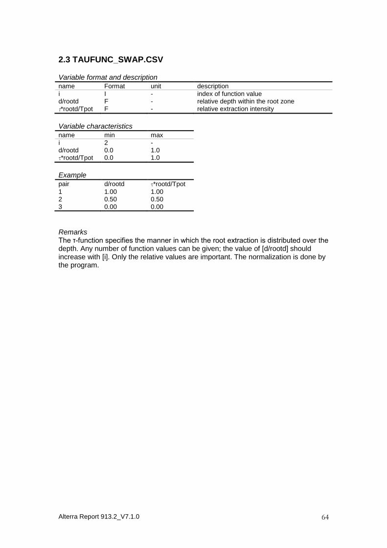
Alterra Report 913.2_V7.1.0 64
2.3 TAUFUNC_SWAP.CSV
Variable format and descriptionname Format unit descriptioni I - index of function valued/rootd F - relative depth within the root zoneτ*rootd/Tpot F - relative extraction intensity
Variable characteristicsname min maxi 2 -d/rootd 0.0 1.0τ*rootd/Tpot 0.0 1.0
Examplepair d/rootd τ*rootd/Tpot1 1.00 1.002 0.50 0.503 0.00 0.00
RemarksThe τ-function specifies the manner in which the root extraction is distributed over the depth. Any number of function values can be given; the value of [d/rootd] shouldincrease with [i]. Only the relative values are important. The normalization is done bythe program.
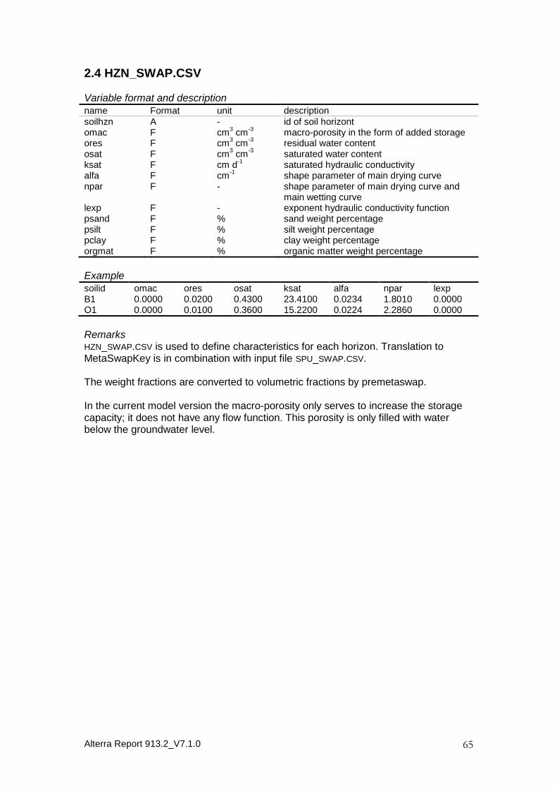
Alterra Report 913.2_V7.1.0 65
2.4 HZN_SWAP.CSV
Variable format and descriptionname Format unit descriptionsoilhzn A - id of soil horizontomac F cm
3cm
-3macro-porosity in the form of added storage
ores F cm3
cm-3
residual water contentosat F cm
3cm
-3saturated water content
ksat F cm d-1
saturated hydraulic conductivityalfa F cm
-1shape parameter of main drying curve
npar F - shape parameter of main drying curve andmain wetting curve
lexp F - exponent hydraulic conductivity functionpsand F % sand weight percentagepsilt F % silt weight percentagepclay F % clay weight percentageorgmat F % organic matter weight percentage
Examplesoilid omac ores osat ksat alfa npar lexpB1 0.0000 0.0200 0.4300 23.4100 0.0234 1.8010 0.0000O1 0.0000 0.0100 0.3600 15.2200 0.0224 2.2860 0.0000
RemarksHZN_SWAP.CSV is used to define characteristics for each horizon. Translation toMetaSwapKey is in combination with input file SPU_SWAP.CSV.
The weight fractions are converted to volumetric fractions by premetaswap.
In the current model version the macro-porosity only serves to increase the storagecapacity; it does not have any flow function. This porosity is only filled with waterbelow the groundwater level.
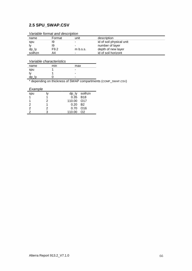
Alterra Report 913.2_V7.1.0 66
2.5 SPU_SWAP.CSV
Variable format and descriptionname Format unit descriptionspu I9 - id of soil physical unitly I9 - number of layerdp_ly F9.2 m b.s.s. depth of new layersoilhzn A4 - id of soil horizont
Variable characteristicsname min maxspu 1 -ly 1 -dp_ly 0 -
* depending on thickness of SWAP compartments (COMP_SWAP.CSV)
Examplespu ly dp_ly soilhzn1 1 0.35 B181 2 110.00 O172 1 0.20 B22 2 0.70 O162 3 110.00 O2
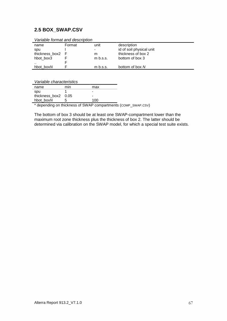
Alterra Report 913.2_V7.1.0 67
2.5 BOX_SWAP.CSV
Variable format and descriptionname Format unit descriptionspu I - id of soil physical unitthickness_box2 F m thickness of box 2hbot_box3 F m b.s.s. bottom of box 3.. Fhbot_boxN F m b.s.s. bottom of box N
Variable characteristicsname min maxspu 1 -thickness_box2 0.05 -hbot_boxN 5 100
* depending on thickness of SWAP compartments (COMP_SWAP.CSV)
The bottom of box 3 should be at least one SWAP-compartment lower than themaximum root zone thickness plus the thickness of box 2. The latter should bedetermined via calibration on the SWAP model, for which a special test suite exists.

Alterra Report 913.2_V7.1.0 68
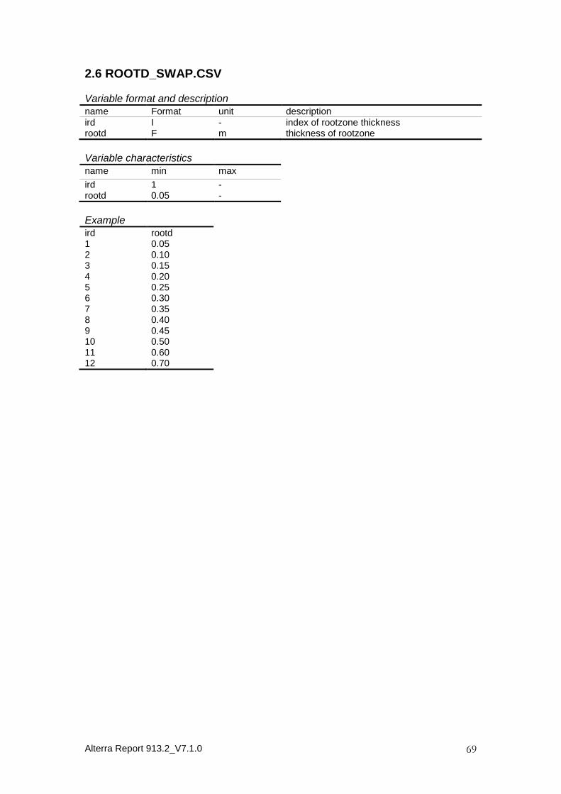
Alterra Report 913.2_V7.1.0 69
2.6 ROOTD_SWAP.CSV
Variable format and descriptionname Format unit descriptionird I - index of rootzone thicknessrootd F m thickness of rootzone
Variable characteristicsname min max
ird 1 -rootd 0.05 -
Exampleird rootd1 0.052 0.103 0.154 0.205 0.256 0.307 0.358 0.409 0.4510 0.5011 0.6012 0.70
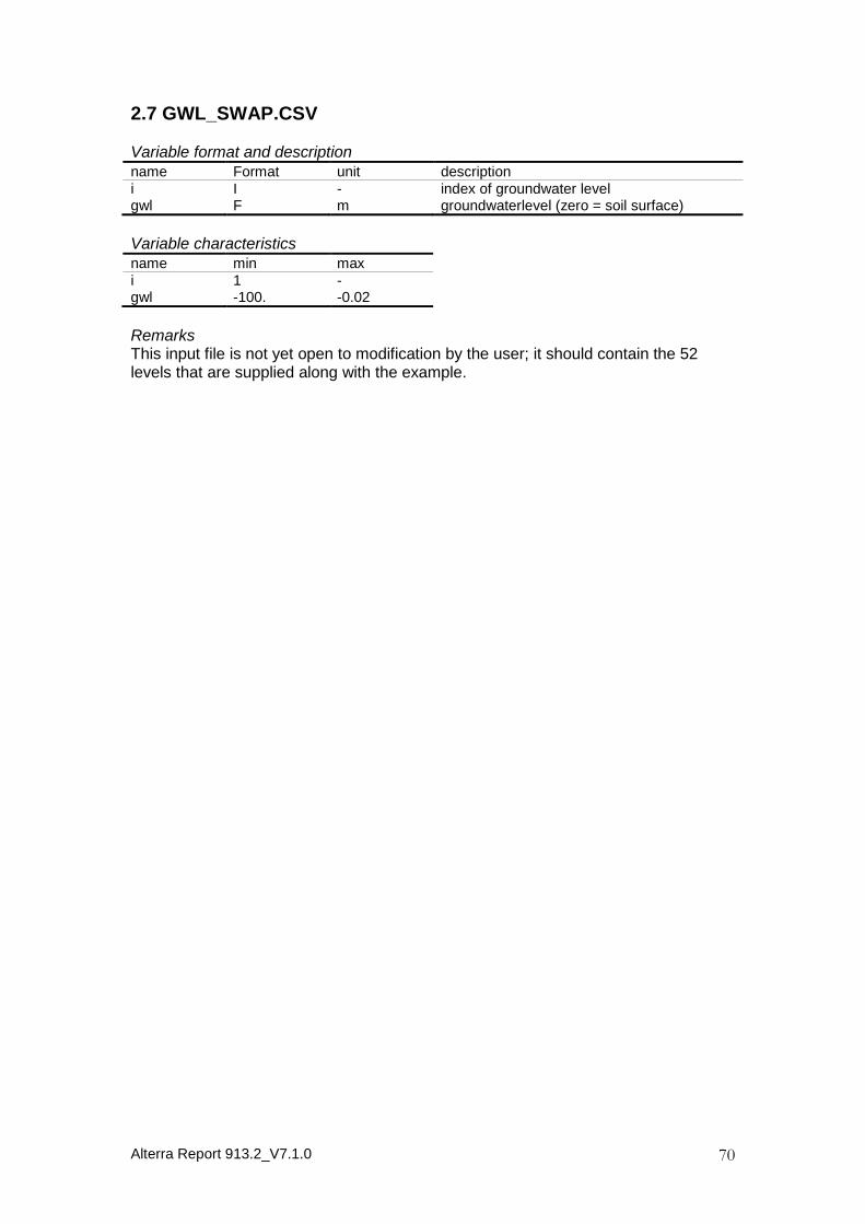
Alterra Report 913.2_V7.1.0 70
2.7 GWL_SWAP.CSV
Variable format and descriptionname Format unit descriptioni I - index of groundwater levelgwl F m groundwaterlevel (zero = soil surface)
Variable characteristicsname min maxi 1 -gwl -100. -0.02
RemarksThis input file is not yet open to modification by the user; it should contain the 52levels that are supplied along with the example.
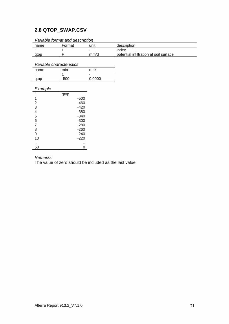
Alterra Report 913.2_V7.1.0 71
2.8 QTOP_SWAP.CSV
Variable format and descriptionname Format unit descriptioni I - indexqtop F mm/d potential infiltration at soil surface
Variable characteristicsname min maxi 1 -qtop -500 0.0000
Examplei qtop1 -5002 -4603 -4204 -3805 -3406 -3007 -2808 -2609 -24010 -220.. ..50 0
RemarksThe value of zero should be included as the last value.
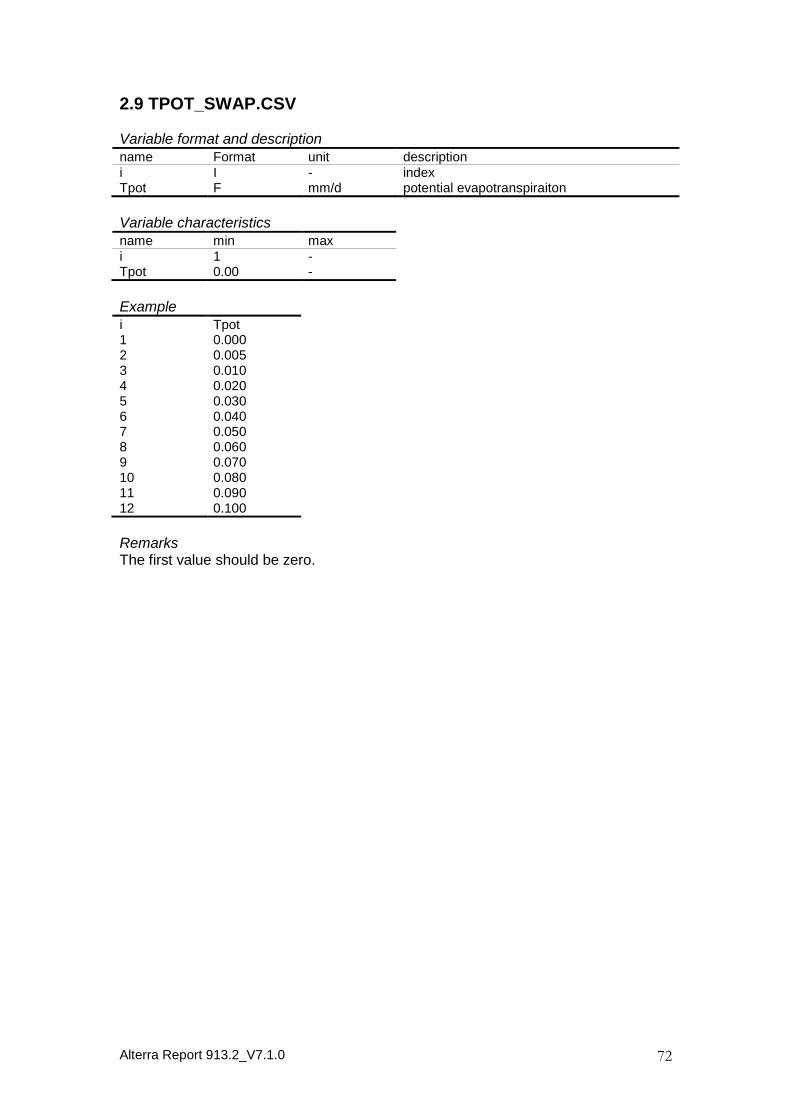
Alterra Report 913.2_V7.1.0 72
2.9 TPOT_SWAP.CSV
Variable format and descriptionname Format unit descriptioni I - indexTpot F mm/d potential evapotranspiraiton
Variable characteristicsname min maxi 1 -Tpot 0.00 -
Examplei Tpot1 0.0002 0.0053 0.0104 0.0205 0.0306 0.0407 0.0508 0.0609 0.07010 0.08011 0.09012 0.100
RemarksThe first value should be zero.
Alterra Report 913.2_V7.1.0 73
3 Output files
The output files UNSA*.* are documented in the IO-manual. An example is availablevia the ftp-site of Alterra.
The binary files (*.BDA) are the preferred option to use in combination with the model,because the access is much faster. However, the SIMGRO program should becompiled with the same Fortran compiler as the PreMetaSWAP, otherwiseincompatibility can occur. In that case the ASCII files (*.INP) can be used instead.These files are also useful for inspecting the data. If the file is too large for loading inmemory, then the head of the file should be transferred to a .TMP file by shortlyrunning the type command in a dos-box, and redirecting the output with ‘>’.
The CSV-files contain the simulated profiles.

Alterra Report 913.2_V7_0_0 74

Alterra Report 913.2_V7_0_0 75
Appendix B PostMetaSWAP
1 Program use
PostMetaSWAP2TRANSOL is a program that disaggregates the output ofMODFLOW-SIMGRO. The default output consists of a series of SWATRE*.UNF
files that can be used in water quality simulations.
To run the program the files listed in Table 1 should be available.
Table 1.1. List of input files
Name fo file DescriptionUNSA_POST.BDA extended database produced by PreMetaSWAPSVAT_PER.UNF database file produced by MODFLOW-SIMGRO
by setting the svat_per_unf parameter to 1 inPARA_SIM.INP (undocumented file)
COMP_POST.CSV list of desired compartment thicknesses in verticalprofile (see Section 2.1 of this Appendix)
SEL_SVAT.INP selection of SVAT’s that should actually beprocessed (see Section 2.2 of this Appendix)
SEL_SVAT_CSV.INP selection of SVAT’s for which extra output will besupplied in the form of csv files of head, moisturecontent, and temperature
WRITECONTROL.INP file for control of programme action (examplegiven below)
The program produces by default the output files listed in Table 2. An example ofthe WRITECONTROL.INP file:
------------------------------------------------------------------------------------------------------------.true. ! write2file : optional output to SWATRE.* files.false. ! dotransol : optional simulation of transport of solutes.true. ! dotemp : optional simulation of temperature" " ! unsa_path : path of soil database; “ “ = work dir; end path with “\”
------------------------------------------------------------------------------------------------------------
Table 1.2. List of output filesName fo file DescriptionSWATRE_*.UNF unformatted files per MetaSWAP columns, with
disgaggregated moistire profilesSWATRE_*.OUT ascii version of files
The running of the programme is done automatically in the T-Model example(Appendix C).

Alterra Report 913.2_V7_0_0 76
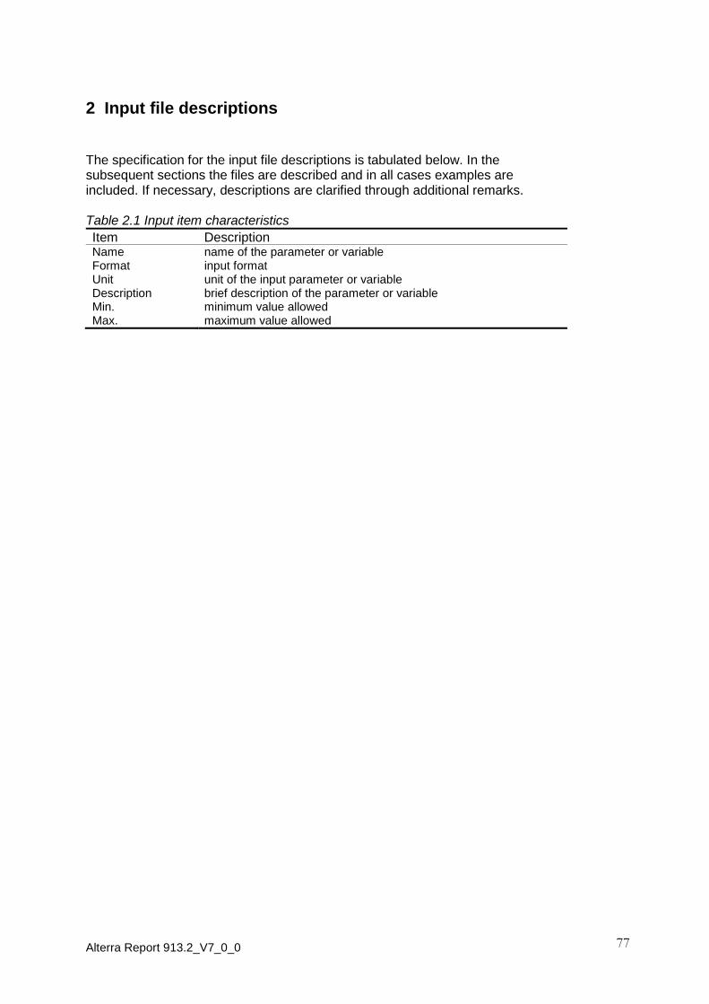
Alterra Report 913.2_V7_0_0 77
2 Input file descriptions
The specification for the input file descriptions is tabulated below. In thesubsequent sections the files are described and in all cases examples areincluded. If necessary, descriptions are clarified through additional remarks.
Table 2.1 Input item characteristics
Item DescriptionName name of the parameter or variableFormat input formatUnit unit of the input parameter or variableDescription brief description of the parameter or variableMin. minimum value allowedMax. maximum value allowed
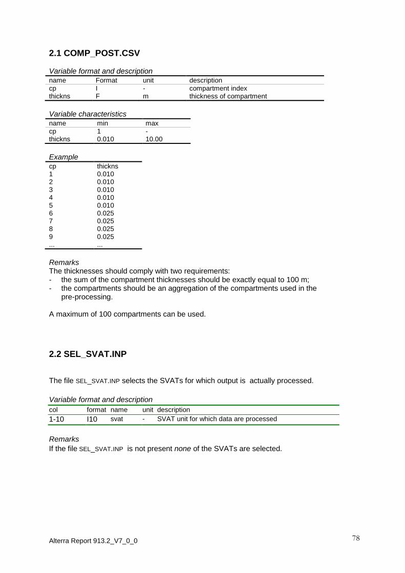
Alterra Report 913.2_V7_0_0 78
2.1 COMP_POST.CSV
Variable format and descriptionname Format unit descriptioncp I - compartment indexthickns F m thickness of compartment
Variable characteristicsname min maxcp 1 -thickns 0.010 10.00
Examplecp thickns1 0.0102 0.0103 0.0104 0.0105 0.0106 0.0257 0.0258 0.0259 0.025... ...
RemarksThe thicknesses should comply with two requirements:- the sum of the compartment thicknesses should be exactly equal to 100 m;- the compartments should be an aggregation of the compartments used in the
pre-processing.
A maximum of 100 compartments can be used.
2.2 SEL_SVAT.INP
The file SEL_SVAT.INP selects the SVATs for which output is actually processed.
Variable format and description
col format name unit description
1-10 I10 svat - SVAT unit for which data are processed
Remarks
If the file SEL_SVAT.INP is not present none of the SVATs are selected.

Alterra Report 913.2_V7_0_0 79
3 Output files
The format of the SWATRE*.* output files is described in the ANIMO manual,included in the docs-subdirectory of SIMGRO and the T-Model-Basic example.

Alterra Report 913.2_V7_0_0 80

Alterra Report 913.2_V7_0_0 81
Appendix C Demonstration dataset
1 T-model_Basic
The so-called T-model_Basic has a rectangular model area, involving 110 SVATunits as numbered in Figure 1. The SVATs are mapped to surface water locations1-21. But these locations are not coupled to a surface water model in this basicexample. That means that if there is demand of sprinkling from one of theselocations, the supply is assumed to always be available.
The data of the demo-set have been structured with the following subrdirectories(alphabetical order):- apr, with the ArcView project file;- bat, with the command files; the model can be run by simply double-clicking
on the modflow-simgro.bat file;- cov, with the shape files and grids;- exe, with the executables- inp_modflow and inp_simgro, with the input files- log, with the log files;- out_modflow and out_simgro with the output filesThe out_simgro subdirectory has four subdirectories:- asc, with the grids that can be imported;- bda, with the output database files;- csv, with the output csv-files;- unf, with the disaggregated soil moistire profiles for use by water quality
models
1 2 3 4 5 6 7 8 9
51
10
999897969594939291
90898887868584838281
80797877767574737271
70696867666564636261
605958575655545352
11
50494847464544434241
40393837363534333231
30292827262524232221
201918171615141312
101
100
102 103 104 105 106 107 108 109 110
Figure 1. SVAT units
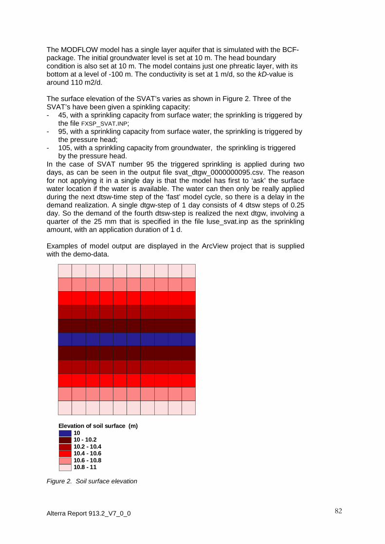
Alterra Report 913.2_V7_0_0 82
The MODFLOW model has a single layer aquifer that is simulated with the BCF-package. The initial groundwater level is set at 10 m. The head boundarycondition is also set at 10 m. The model contains just one phreatic layer, with itsbottom at a level of -100 m. The conductivity is set at 1 m/d, so the kD-value isaround 110 m2/d.
The surface elevation of the SVAT’s varies as shown in Figure 2. Three of theSVAT’s have been given a spinkling capacity:- 45, with a sprinkling capacity from surface water; the sprinkling is triggered by
the file FXSP_SVAT.INP;- 95, with a sprinkling capacity from surface water, the sprinkling is triggered by
the pressure head;- 105, with a sprinkling capacity from groundwater, the sprinkling is triggered
by the pressure head.In the case of SVAT number 95 the triggered sprinkling is applied during twodays, as can be seen in the output file svat_dtgw_0000000095.csv. The reasonfor not applying it in a single day is that the model has first to ‘ask’ the surfacewater location if the water is available. The water can then only be really appliedduring the next dtsw-time step of the ‘fast’ model cycle, so there is a delay in thedemand realization. A single dtgw-step of 1 day consists of 4 dtsw steps of 0.25day. So the demand of the fourth dtsw-step is realized the next dtgw, involving aquarter of the 25 mm that is specified in the file luse_svat.inp as the sprinklingamount, with an application duration of 1 d.
Examples of model output are displayed in the ArcView project that is suppliedwith the demo-data.
Elevation of soil surface (m)1010 - 10.210.2 - 10.410.4 - 10.610.6 - 10.810.8 - 11
Figure 2. Soil surface elevation


![Alcatel-Lucent 1354 BM-ATM | Release 7.1 Installation Guide · Edition: the 6th delivery [2] Os-Kernel Customization/Administration Guide ... [6] SWP-OSCONF-V7.1.0 …](https://img.pdfslide.us/doc/110x75/5b227d1a7f8b9a9c438b45a3/alcatel-lucent-1354-bm-atm-release-71-installation-guide-edition-the-6th.jpg)