Significance of model credibility in estimating climateprojection distributions for regional hydroclimatologicalrisk assessments

Levi D. Brekke & Michael D. Dettinger &

Edwin P. Maurer & Michael Anderson

Received: 1 December 2006 /Accepted: 6 November 2007 / Published online: 28 February 2008# Springer Science + Business Media B.V. 2007

Abstract Ensembles of historical climate simulations and climate projections from theWorld Climate Research Programme’s (WCRP’s) Coupled Model Intercomparison Projectphase 3 (CMIP3) multi-model dataset were investigated to determine how model credibilityaffects apparent relative scenario likelihoods in regional risk assessments. Methods weredeveloped and applied in a Northern California case study. An ensemble of 59 twentiethcentury climate simulations from 17 WCRP CMIP3 models was analyzed to evaluaterelative model credibility associated with a 75-member projection ensemble from the same17 models. Credibility was assessed based on how models realistically reproduced selectedstatistics of historical climate relevant to California climatology. Metrics of this credibilitywere used to derive relative model weights leading to weight-threshold culling of modelscontributing to the projection ensemble. Density functions were then estimated for twoprojected quantities (temperature and precipitation), with and without consideringcredibility-based ensemble reductions. An analysis for Northern California showed that,while some models seem more capable at recreating limited aspects twentieth centuryclimate, the overall tendency is for comparable model performance when several credibilitymeasures are combined. Use of these metrics to decide which models to include in densityfunction development led to local adjustments to function shapes, but led to limited affect

Climatic Change (2008) 89:371–394DOI 10.1007/s10584-007-9388-3

L. D. Brekke (*)Technical Service Center 86-68520, U.S. Bureau of Reclamation, Denver, CO 80225-0007, USAe-mail: lbrekke@do.usbr.gov

M. D. DettingerU.S. Geological Survey and Scripps Institution of Oceanography, La Jolla, CA 92093-0224, USAe-mail: mddettin@usgs.gov

E. P. MaurerCivil Engineering Department, Santa Clara University, Santa Clara, CA 95053-0563, USAe-mail: emaurer@engr.scu.edu

M. AndersonDivision of Flood Management, California Department of Water Resources, Sacramento,CA 95821-9000, USAe-mail: manderso@water.ca.gov

on breadth and central tendency, which were found to be more influenced by“completeness” of the original ensemble in terms of models and emissions pathways.

1 Introduction

Resource managers currently face many questions related to potential climate changes, inparticular how climate may change and what regional impacts would ensue. One of themost pressing questions is whether contemporary resource-management decisions mightincrease or decrease future impacts. To address these questions, analysts typically compileglobal climate projections and then spatially downscale them for impacts assessment atregional scales relevant to a given decision. Given that there are more than 20 globalclimate models currently in operation, producing simulations of future climate under severaldifferent greenhouse gas (GHG) emission scenarios (Meehl et al. 2005), it is not surprisingthat results drawn from such impacts assessments depend on the particular GHG forcingscenarios and climate models present in these compilations.

Focusing on a few projected scenarios (e.g., bookend analyses) can lead to significantdivergence among the projected future impacts. While such analyses are useful forillustrating what may be at stake under different future scenarios, they provide limitedguidance for management responses in the present (e.g., Brekke et al. 2004; Cayan et al.2006; Hayhoe et al. 2004; Vicuna et al. 2007). Rather, it is important for managers tounderstand the distributed and consensus nature of projected climate change impacts(Dettinger 2005; Maurer 2007) so that managers can begin to consider the relativelikelihood of future impacts rather than just isolated examples of potential impacts. In linewith this philosophy, there has been a trend in recent impacts assessments to base thestudies on larger multi-model projection ensembles, as for instance in recent studies ofpotential hydrologic impacts in California’s Central Valley (Maurer and Duffy 2005;Maurer 2007), the Colorado River Basin (Milly et al. 2005; Christensen and Lettenmaier2006), and in other locations (Wilby and Harris 2006; Zierl and Bugmann 2005).

Expanding regional impacts analyses to consider larger climate projection ensemblescreates the opportunity to address and communicate impacts in the terms of risks rather thanisolated examples of possible impacts. The difference between risk and impact assessmentsis that risk goes beyond scenario definition and analysis of associated impacts to alsoaddress relative scenario likelihoods. Framing regional assessments in terms of risk isattractive from a management perspective because risk information is better suited forstrategic planning, where responses can be formulated based upon weighted prospects ofdifferent impacts. This approach helps to guide the timely use of limited available fundsthat might support responses to inherently uncertain future conditions.

The product of a risk analysis is a presentation of distributed impacts from a collectionof scenarios weighted by their estimated likelihoods. In the climate change context,absolute scenario likelihoods cannot be identified. However, relative- or consensus-basedlikelihoods of various scenarios can be estimated from an ensemble of climate projectionsby fitting a climate projection density function. Granted, such density functions onlyrepresent a limited portion of the climate change uncertainties, because elements such associal and physical factors affecting global GHG sources and sinks in the future, climateresponse and interactions with these GHG sources and sinks, and alternative climate modelstructures are not included. However, the ensemble density functions provide a morecomplete basis for using and interpreting the elements of the available ensembles than isafforded by scenario analyses without such context. Using projection density functions to

372 Climatic Change (2008) 89:371–394

infer relative scenario likelihoods promotes strategic response planning, framed by perceptionof which outcomes are – at present – projected to be more likely among projectedpossibilities, which is a step forward from not considering scenario likelihoods at all.

Several methods for generating climate projections density functions have beenproposed (Tebaldi et al. 2005; Dettinger 2006). The ensembles employed can includeseveral greenhouse gas emission pathways, multiple climate models, and multiple “runs” ofa given pathway-model combination differing by initial conditions. In applying thesemethodologies, it is natural to ask whether all members from a projection ensemble shouldbe valued equally. Put another way, there are more than 20 coupled atmosphere–oceanclimate models informing the last assessment from IPCC (2007): in the context of regionalresponse analysis, are the projections from all of these models equally credible?

This latter thought motivates the two questions considered in this paper: (1) How doesapparent model credibility at a regional scale, translated into relative model weighting andsubsequent model culling, affect estimates of climate projection density functions?, and(2) How are relative scenario likelihoods, derived from the density function, affected whenmodel credibility is considered when estimating the function?

To explore the first question, a philosophy is adopted that relative model credibility inprojecting twenty-first century climate can be estimated from relative model accuracy insimulating twentieth century climate. Some studies have found little effect of weighting futureclimate projections by perceived differences between model completeness (e.g., Dettinger2005, weighted models based on whether they required “flux corrections” or not to avoidclimate drift and found little difference in estimated density functions). However, severalinterpretations of projection ensembles have been designed around the concept of weightingresults by perceived historical accuracies (AchutaRao and Sperber 2002, 2006; Bader et al.2004; Phillips et al. 2006). Following this approach, a procedure is developed here, beginningwith a model credibility analysis to produce relative model credibility indices, as a basis formodel culling, followed by a nonparametric procedure for estimating climate projectiondensity functions, with and without consideration of model credibility results.

In the latter step, an “Uncertainty Ensemble” of climate projections is used to fit thedensity functions. In relation to the second question, a subset of the Uncertainty Ensembleis identified (i.e. Impacts Ensemble) for which relative scenario weights are derived fromthe density functions fit with and without consideration of model credibility. The nestednature of this Impacts Ensemble within the Uncertainty Ensemble represents a typicalsituation in regional risk assessment where the feasible size of an Impacts Ensemble (i.e.scenarios studied in detail for impacts in multiple resource areas) is less than what can beconsidered when fitting the climate projection density function because of the computa-tional intensity of the impact calculations. The remainder of this paper presents themethodologies for model credibility and climate projection density analyses (section 2),results from applying these methods to a particular region (i.e. California’s Central Valley)where the concern is water resources impacts (section 3), a discussion of method limitationsand areas of potential improvement (section 4), and a summary of major conclusions(section 5).

2 Methodology

The analytical sequence features two primary parts. The first part involves a modelcredibility analysis based on how well selected parts of the historical climate are simulatedby the various models, and includes the following steps: (1) choosing relevant climate

Climatic Change (2008) 89:371–394 373

variables and reference data, (2) choosing performance metrics and computing measures ofmodel-to-observation similarities, and (3) deriving weights and culled model groups basedon these measures. The second part is an analysis of climate projections where projectiondensity functions are fit with and without consideration of results from the model credibilityanalysis.

The analyses are based on simulated climate variables from coupled atmosphere–oceangeneral circulation models (i.e. WCRP CMIP3 models) used to produce (a) twenty-firstcentury climate projections under both SRES A2 and B1 emissions pathways (IPCC 2001)and (b) simulations for the “climate of the twentieth century experiment (20C3M),”conducted by CMIP3 participants (Covey et al. 2003). The Lawrence Livermore NationalLaboratory’s Program for Climate Model Diagnosis and Intercomparison (PCMDI) hosts amulti-model archive for 20C3M historical simulations, twenty-first century projections, andother scenario and control run datasets. Among the models producing 20C3M simulations,the number of available “runs” varied per model, with runs differing by initializationdecisions. An attempt was made to focus on models that had simulated both A2 and B1 onthe grounds that these pathways represent a broad and balanced range of SRES possibilities(IPCC 2001). However, this criterion was relaxed for two of the selected models fromwhich only A2 or B1 simulations were available.

In total, 17 climate models were represented in our survey (Table 1). Collectively theywere used to produce 59 20C3M simulations (used for the model credibility analysis) and75 climate projections comprised of 37 SRES A2 simulations and 38 SRES B1 simulations.The set of 75 climate projections served as the Uncertainty Ensemble, mentioned insection 1, and was used in climate projection density analysis. From the UncertaintyEnsemble, subsets of 11 SRES A2 and 11 SRES B1 projections were identified as a22-member Impacts Ensemble (Table 1). The selected 22 projections are the sameprojections considered in a previous study on potential hydrologic impacts uncertaintywithin the Sierra Nevada (Maurer 2007).

2.1 Credibility analysis: choosing simulated and references climate variables

The first step in the model credibility analysis involved choosing simulated climate variablesrelevant to the geographic region of interest (i.e. Northern California in this case study), andidentifying climate reference data to which simulated historical climates could be compared(i.e. 20C3M results listed in Table 1). Three types of variables were used: local variables thatdefine Northern California climatology, distant variables that characterize global-scaleclimatic processes, and variables that describe how global processes relate to the localclimatology (i.e. teleconnections). This mix was chosen because the first interest for thisregional scale assessment was how the local climate variables might change in the future.However, in the projections considered here, those changes are driven and established byglobal scale forcings (GHGs) and resulting processes. Thus, both local and globalperformances are important. Furthermore, the connection between global and local processesmust be accurately recreated in the models (indicated by either the presence or absence ofsignificant inter-variable correlation, i.e. teleconnections) in order for their simulated localresponses to global forcings to be considered reliable.

Two local variables were used to describe the regional climatology: surface airtemperature and precipitation conditions (i.e. NorCalT and NorCalP near {122W, 40N}).Global-scale phenomena driving the regional climatology via teleconnections includepressure conditions over the North Pacific (related to mid-latitude storm track activityupwind of North America) and the phase of the El Niño Southern Oscillation (ENSO;

374 Climatic Change (2008) 89:371–394

affecting Pacific-region interannual climate variability and beyond). Two measures of thesephenomena were used in this study, respectively: the North Pacific Index (NPI), describingmean sea level pressure within {30N–65N, 160E–140W} and the Nino3 Index describingENSO-related mean sea surface temperature within {5S–5N, 150W–90W}.

Monthly time series of each evaluation variable were extracted from each 20C3Msimulation for the latter half of the twentieth century (1950–1999). Likewise, monthly1950–1999 “reference” data were also obtained. For NPI, NorCalP, and NorCalT, thereference data were extracted from the NCEP Reanalysis (Kalnay et al. 1996, updated andprovided by the NOAA/OAR/ESRL PSD, Boulder, Colorado, USA, from their Web site athttp://www.cdc.noaa.gov/), which is a data set of historical observations modified andinterpolated with the use of an atmospheric climate model and which describes climateconditions at roughly the same scale as the coupled climate models used in the historicalsimulations. The reference data for Nino3 were obtained from the Monthly Atmosphericand SST Indices archive provided by the NWS Climate Prediction Center, Camp Springs,Maryland, USA, from their Web site at http://www.cpc.noaa.gov/data/indices/.

Simulated and reference time series were compared during the 1950–1999 period. It isarguable whether this 50-year historical period should be shorter and more recent. Thedecision to consider 1950–1999 as opposed to a shorter period was driven by recognitionthat 20C3M simulations express interdecadal variability that might be out of phase with that

Table 1 Climate projections and models included in this case study

WCRP CMIP3model I.D.a

Model abbreviation inthis study

Modelnumber

Projection run numbersb 20C3mEnsemble

Uncertainty Impacts

A2 B1 A2 B1

CGCM3.1(T47) cccma_cgcm31 1 1…5 1…5 1…5CNRM-CM3 cnrm_cm3 2 1 1 1 1 1CSIRO-Mk3.0 csiro_mk30 3 1 1 1 1 1…3GFDL-CM2.0 gfdl_cm20 4 1 1 1 1 1…3GFDL-CM2.1 gfdl_cm21 5 1 1 1…3GISS-ER giss_model_er 6 1 1 1 1 1…9INM-CM3.0 inmcm3_0 7 1 1 1 1 1IPSL-CM4 ipsl_cm4 8 1 1 1 1 1MIROC3.2(hires) miroc32_hires 9 1 1MIROC3.2(medres) miroc32_medres 10 1…3 1…3 1 1 1…3ECHAM5/MPI-OM mpi_echam5 11 1…3 1…3 1 1 1…3MRI-CGCM2.3.2 mri_cgcm232a 12 1…5 1…5 1 1 1…5CCSM3 ncar_ccsm30 13 1…5 1…8 1…8PCM ncar_pcm1 14 1…4 2…3 1 2 1…4UKMO-HadCM3 ukmo_hadcm3 15 1 1 1 1 1…2UKMO-HadGEM1 ukmo_hadgem1 16 1 1…2ECHO-G miub echo-g 17 1…3 1…3 1…5Total Runs 37 38 11 11 59

a From information at Lawrence Livermore National Laboratory’s Program for Climate Model Diagnosisand Intercomparison (PCMDI), September 2006: http://www-pcmdi.llnl.govb Run numbers assigned to model- and pathway-specific SRES projections and model-specific 20c3msimulations in the WCRP CMIP3 multi-model data archive at PCMDI.

Climatic Change (2008) 89:371–394 375

observed during the twentieth century, leading to exaggerated simulation-referencedifferences or similarities based solely on choice of sampling overlap period.

2.2 Credibility analysis: choosing performance metrics and teleconnections

The next step was to choose performance metrics that describe statistical aspects of thelocal and global variables and their teleconnections. For each variable, a set of six metricswas evaluated (Table 2): the first three statistical moments of annual conditions (mean,variance, skewness), an interdecadal variance describing lower frequency variability(Table 2, note 4), amplitude of seasonality defined by the range of mean monthlies, andphase of seasonality defined by correlation between simulated and reference meanmonthlies. For the local variables (i.e. NorCalT and NorCalP), the characteristics ofextreme positive anomalies were considered (i.e. the annual maximum monthly valueexceeded in 10% of years). Seasonal correlations (teleconnections) between the two localand two global variables were considered, as well as seasonal and annual correlationsbetween the two global variables. For NorCalT, the 50-year trend was used as an additionalvariable-specific metric. For NorCalP, a metric of drought recurrence and severity was alsoincluded and framed by knowledge of relevant 1950–1999 droughts in the case studyregion. Because the most significant sustained drought in the Northern Californiainstrumental record was about 6 years in duration (1987–1992), the drought metric wasdefined as the running 6-year precipitation total exceeded by 90% of the 6-year spellswithin each 50-year time series. Finally, as a measure of how temporally realistic thesimulated ENSO processes were, and because local interannual variability is influenced byENSO, a metric describing El Niño reoccurrence was defined as the spectral power of the50-year Nino3 time series concentrated in the 2-to-7 year range.

This is a fairly extensive array of metrics, and it is difficult to know which of the metricsare most pertinent to the projection of future impacts of increasing GHGs. Application ofthis methodology thus will involve consideration of which metrics are the most relevantmeasures of model credibility. In applications of this approach to other regions, decisions toinclude other, or additional, metrics beyond those discussed herein should depend on theregion and climate in question. Although no definitive statements can be made as to whichmetrics are the more relevant, it is reasonable to expect that different impacts assessmentperspectives might gravitate toward different metrics. For illustration purposes, threeperspectives are defined and used here to explore sensitivity of impressions to this question.The perspectives are loosely termed Water Supply, Hydropower, and Flood Control. Foreach perspective, the 49 metrics of Table 2 were reduced to six arbitrarily chosen metrics asbeing “more relevant.”

– For the Water Supply perspective, managers are assumed to have the ability toseasonally store precipitation-runoff and thus might be more concerned about howclimate models reproduce the past precipitation in terms of long-term mean andseasonality phase, past temperature in terms of long-term trend and seasonality phase,multi-year drought severity, and global teleconnections relevant to the precipitationseason (e.g., Nino3-NorCalP during Winter).

– For the Hydropower perspective, concerns were assumed to be similar to those ofWater Supply (e.g., precipitation long-term mean, temperature long-term trend), butwith more concern shifted to other types of global teleconnections with local climate(e.g., NPI correlation with NorCalP during autumn and winter) and on globalinterannual variability in general as it might affect hydro-energy resources from a larger

376 Climatic Change (2008) 89:371–394

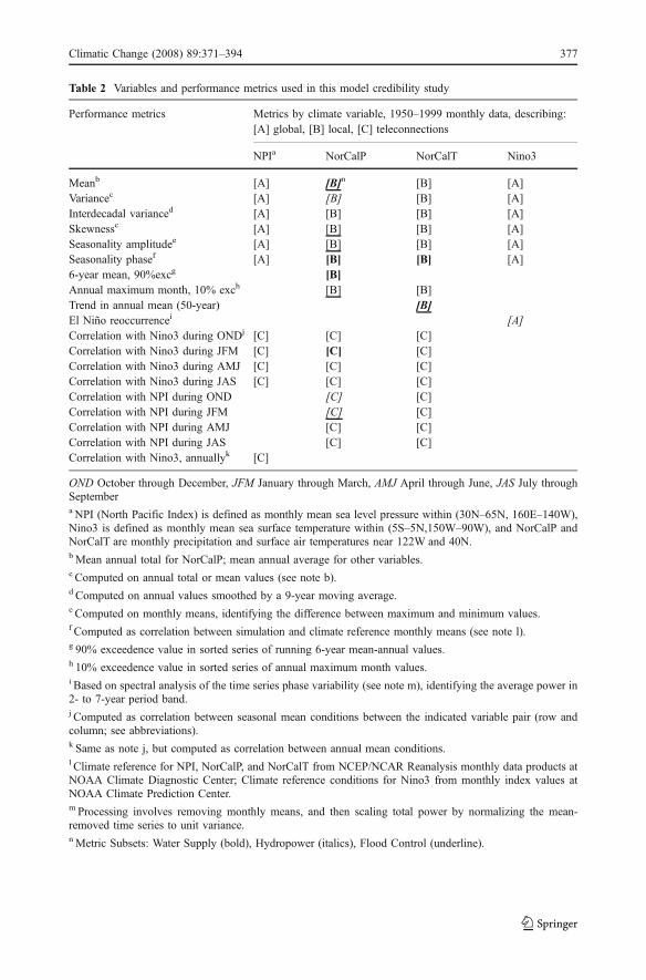
Table 2 Variables and performance metrics used in this model credibility study

Performance metrics Metrics by climate variable, 1950–1999 monthly data, describing:[A] global, [B] local, [C] teleconnections

NPIa NorCalP NorCalT Nino3

Meanb [A] [B]n [B] [A]Variancec [A] [B] [B] [A]Interdecadal varianced [A] [B] [B] [A]Skewnessc [A] [B] [B] [A]Seasonality amplitudee [A] [B] [B] [A]Seasonality phasef [A] [B] [B] [A]6-year mean, 90%excg [B]Annual maximum month, 10% exch [B] [B]Trend in annual mean (50-year) [B]El Niño reoccurrencei [A]Correlation with Nino3 during ONDj [C] [C] [C]Correlation with Nino3 during JFM [C] [C] [C]Correlation with Nino3 during AMJ [C] [C] [C]Correlation with Nino3 during JAS [C] [C] [C]Correlation with NPI during OND [C] [C]Correlation with NPI during JFM [C] [C]Correlation with NPI during AMJ [C] [C]Correlation with NPI during JAS [C] [C]Correlation with Nino3, annuallyk [C]

OND October through December, JFM January through March, AMJ April through June, JAS July throughSeptembera NPI (North Pacific Index) is defined as monthly mean sea level pressure within (30N–65N, 160E–140W),Nino3 is defined as monthly mean sea surface temperature within (5S–5N,150W–90W), and NorCalP andNorCalT are monthly precipitation and surface air temperatures near 122W and 40N.bMean annual total for NorCalP; mean annual average for other variables.c Computed on annual total or mean values (see note b).d Computed on annual values smoothed by a 9-year moving average.e Computed on monthly means, identifying the difference between maximum and minimum values.f Computed as correlation between simulation and climate reference monthly means (see note l).g 90% exceedence value in sorted series of running 6-year mean-annual values.h 10% exceedence value in sorted series of annual maximum month values.i Based on spectral analysis of the time series phase variability (see note m), identifying the average power in2- to 7-year period band.j Computed as correlation between seasonal mean conditions between the indicated variable pair (row andcolumn; see abbreviations).k Same as note j, but computed as correlation between annual mean conditions.l Climate reference for NPI, NorCalP, and NorCalT from NCEP/NCAR Reanalysis monthly data products atNOAA Climate Diagnostic Center; Climate reference conditions for Nino3 from monthly index values atNOAA Climate Prediction Center.m Processing involves removing monthly means, and then scaling total power by normalizing the mean-removed time series to unit variance.n Metric Subsets: Water Supply (bold), Hydropower (italics), Flood Control (underline).

Climatic Change (2008) 89:371–394 377

regional hydropower market encompassing the runoff region of interest (e.g., Nino3 ElNiño reoccurrence).

– For the Flood Control perspective, more focus was assumed to be placed on how theclimate models recreate more extreme aspects of precipitation climatology (e.g.,precipitation skewness, seasonality amplitude, annual maximum month that isexceeded in 10% of the 50-year evaluation period).

Notably, historical simulations were not rated in terms of whether they reproducedprecipitation trends of the past 50 years. As noted previously, the region in question issubject to large, significant and persistent multidecadal climate fluctuations historically,under the influence of multidecadal climate processes over the Pacific Ocean basin andbeyond (e.g., Mantua et al. 1997; McCabe et al. 2004). Historically the multidecadal PacificOcean influence has resulted in significant and persistent climatological differencesbetween the 1948–1976 period and the 1977–1999 period. Although these long-termdifferences may very well be mostly natural, random and reversible, they have imposed atrend-like character on the Northern California climate during 1950–1999. Even a skillfulcoupled ocean–atmosphere model, initiated much earlier in the nineteenth or twentiethcenturies, would not be expected to reproduce the timing of such natural multidecadalfluctuations in a way that would reproduce the trend-like halving of the 1950–1999 windowconsidered here. Thus the presence or absence of a regionalized precipitation trend inobservations and apparent difference in historical simulated trend did not seem to be a goodmeasure of the simulation skill in the particular study region considered here.

2.3 Credibility analysis: deriving model weights and model culling

After computing simulation metrics, run-specific calculations of simulated-minus-referencemetric differences were pooled by model and averaged to produce 17 model-representativedifferences. A distance-based methodology was then used to measure overall model-to-reference similarities for each set of metrics. Under the distance-based philosophy, adistance is computed within a “similarity space” defined along “metric dimensions.” Forexample, the similarity space could be a seven-dimensional space spanned by the sevenNPI performance metrics, or a 49-dimensional space spanned by all performance metrics inTable 2. Given a space definition, distance can be computed using one of several distanceformulas. Euclidean or Manhattan distance formulas were explored in this study (Black2006), with focus ultimately placed on Euclidean distance. Results were found to beinsensitive to choice of distance formula, primarily because metric differences were scaledto have unit variance across models for each metric, prior to distance calculation, so thatmetric differences generally all had magnitudes near or less than one. Such magnitudesaggregate into similar distances using the Euclidean and Manhattan formulas.

The purpose of scaling metric differences was to prevent metrics measured in large unitsfrom dominating the computed distance (e.g., the El Nino reoccurrence metric differenceshave values on the order of 103 where as the seasonality and teleconnection correlation-metrics have differences on the order of 10−1 to 10−2). A disadvantage of scaling the metricdifferences is that it can exaggerate a metric’s influence on model discrimination eventhough pre-scaled metric differences were quite similar (e.g., simulated NorCalT seasonalityphase and difference from reference).

For a given set of metrics, the procedure results in computation of 17 model-representative distances from references. Relative model weights were then computed as theinverse of this distance. Finally, a threshold weight criterion was used to cull models from

378 Climatic Change (2008) 89:371–394

consideration in the subsequent climate projection density analysis. The model-cullingdepends on the metric set used and the threshold model weight selected to differentiatebetween models that will be retained and those that will not. For illustration, in this study,the weight threshold was defined to be median among the 17 weights, so that the ninehighest weighted models were retained from among the 17 considered.

Looking ahead to the climate projection density analysis, the use of these credibiltiyanalysis results could have involved proportional weighting of the models rather thanculling of models. All models could have been retained and various methods toproportionally represent model contribution in the projection density functions could havebeen used. This alternate approach was explored, with density functions fit usingnonparametric techniques (section 2.4). However, it led to excessively multi-modal,“peaky” density functions, set up by the interspersed positions of fitting data (i.e. specificprojections) from “less credible” models and “more credible” models. and was abandonedfor the culling-based approach used here.

2.4 Climate projection density analysis, with and without model credibility

Density functions were constructed for projected anomalies of 30-year average “annualtotal precipitation” and “annual mean surface air-temperature’ [i.e. d(P) and d(T),respectively], evaluated for the 2010–2039 and 2040–2069 periods relative to a 1950–1999 base period. Several methodologies have been proposed for developing densityfunctions that describe likelihoods of univariate or multivariate climate projections (Tebaldiet al. 2005; Dettinger 2006). An empirical procedure is used here, involving nonparametricdensity estimation using Gaussian kernels (Scott 1992; Wilks 1995) with optimizedbandwidths (Silverman 1986). For the multivariate case of jointly projected anomalies oftemperature and precipitation, a product-kernel extension of the univariate approach is used(Scott 1992)). Nonparametric density estimation has been applied in numerous statistical-hydrology studies (e.g., Lall et al. 1996; Piechota et al. 1998). It will be shown that verysimilar joint density functions are obtained by using another estimation approach (Dettinger2006). The emphasis here is on the common motivation underlying these methods: toconsolidate projection information into distributions that help focus planning attention onensemble consensus rather than extremes (Dettinger 2006), and whether relative modelcredibility should be factored into this consolidation.

A key decision in estimating the density functions was how to deal with the variousnumbers of simulations available from a given pathway-model combination (e.g., modelCCSM3 contributes eight SRES B1 simulations whereas model PCM contributes two). Inthe present study, all simulations from all contributing models have been treated as equals.Just as the culling approach used here could have been replaced with a weighting of all themodels, this assignment of equal weights to all of the simulations could have been replacedby weightings of the contributions from various simulations that avoided overemphasis ofsimulations from the more prolific modeling groups. Such weightings were explored in thisstudy and tended to yield results similar to the distributions shown herein, especially withrespect to the central tendencies and spans of the density functions.

In applications of the product kernel for bivariate density estimation, relative variablescales and choices for variable-specific domain resolution and range can influence results.To account for this influence, each univariate function contributing to the product kernelwas fit to anomalies scaled by their respective standard deviations. After constructing thebivariate density function from these scaled data, the function values relative to each scaledanomaly position were mapped back into their unscaled values.

Climatic Change (2008) 89:371–394 379

380 Climatic Change (2008) 89:371–394

3 Case study results – Northern California

3.1 Credibility analysis

As mentioned in section 2, the case study region for this study was Northern California,leading to the focus on two relevant local climate variables for credibility analysis (NorCalPand NorCalT), two global variables influential on local variables (NPI and Nino3), andrespective global–local teleconnections. Summaries of scaled, model-representative, metricdifferences between simulated 20C3M results and observational references are shown onFig. 1a and b. The figures qualitatively indicate relative differences among models for eachmetric. They do not indicate specific differences for a given model and metric. For example,consider differences between each models’s average-20C3M NPI Mean and Reference NPIMean (Fig. 1a, top row). The figure shows shading that scales from light to dark as themagnitude of a difference increases; the sign of the difference is indicated by “x” fornegative and “o” for positive. Results suggest that “mpi echam5” and “ukmo hadgem”generally did a better job reproducing Reference NPI Mean. As another example, considerthe bottom row of Fig. 1a, which shows that the models consistently underpredicted theReference trend in NorCalT during 1950–1999. However, what isn’t shown on Fig. 1a(because specific differences are not shown) is that all models correctly simulated awarming trend, just not enough warming compared to Reference.

Figure 2 indicates relative model weights derived for each model based on the metricvalues indicated in Table 2 (i.e. All Variables and Metrics, and metric sets related to theWater Supply, Hydropower, and Flood Control perspectives). The latter three sets weredefined and discussed in section 2.2. For the “All Variables and Metrics” case, whichincorporated all 49 metrics in Table 2, the relative model weight varies among models byroughly a factor two. Projections from the “gfdl cm2 0,” “miroc3 2 medres,” and “ncarccsm3 0” models would be granted more credibility in this context (Fig. 2). For the “gfdlcm2 0” and “miroc 3 2 medres” models, their greater weights stem from scoring well inmultiple variable-specific subsets. The greater weight for the “ncar ccsm3 0” model wasobtained more by scoring well in the NorCalP subset. For the three perspectives, whichfocused on considerably fewer metrics, the range of relative model weights grows to afactor of 3 to 4.

Retaining models having weight greater than or equal to the median weight among the17 model-specific values, Table 3 shows groups of retained models based on each set ofmodel weights from Fig. 2. The mix of retained models differs depending on whichvariables were used to decide credibility. This is particularly the case if credibility isdetermined by fewer simulation metrics. The ensemble of coupled climate modelsproviding projections includes fairly wide ranges of credibility when individual metricsare considered, but have more similar credibility when the intercomparison is made across asuite of simulated variables. That is, generally, a model may do very well on one metric butnot another, and overall these differences average out for most model-to-modelcomparisons when several dozen metrics are brought to bear.

The effect on deciding model retention of various choices of metric sets was explored,with a subset of results illustrated on Fig. 3, which shows how model retention varies for

Fig. 1 a Scaled model-specific average difference between multiple 20c3m run results and Reference formetric types [A] and [B] in Table 2. Scaling involves pooling run- and metric-specific differences acrossmodels and scaling collectively to unit variance. Shading shows magnitude of scaled difference, with darkershading showing greater magnitude of difference. “X” and “O” symbols are used to indicate the sign ofdifference from reference. b Similar to a, but for metric type [C] in Table 2

R

Climatic Change (2008) 89:371–394 381

each of the combinatorial possibilities of one- to eight-metric sets from the type [B] metricsassociated with NorCalP (Table 2). Results show that, while model retention varies with themetric set used, some models would be more frequently retained and thus are could beconsidered to be the relatively more credible models for simulating NorCalP (e.g., “ukmohadgem1,” “ncar pcm,” “ncar ccsm3 0,” “miroc3 2 medres,” “ipsl cm4,” “inmcm3 0,” and“gfdl 2 0”). Next generation models (e.g., “gfdl cm 2 1” compared to “gfdl cm 2 0”) andhigher resolution models (e.g., “miroc3 2 hires” compared to “miroc3 2 medres”) do notnecessarily fare better than their predecessors in such credibility evaluations.

3.2 Climate projection density functions

The results from Table 3 were carried forward to the construction of climate projectiondensity functions. Prior to fitting density functions, ensembles of projected time series(Table 1) for surface air temperature and precipitation anomalies, as simulated near {122W,40N}, were extracted from the A2 and B1 simulations retained in the previous step.Anomalies were computed as deviations of the projected monthly values from the model’s1950–1999 20C3M monthly means. Projected anomalies were then bias-corrected toaccount for model tendencies relative to observations on the projected quantities (i.e.NorCalP and NorCalT from Reanalysis). Bias-correction was performed on a month-specific basis by multiplying projected anomalies by the ratio of Reanalysis monthly meansto the model’s 20C3M monthly means. After bias-correction, monthly anomalies wereconsolidated into annual mean surface air temperature anomalies and annual totalprecipitation anomalies for each the 75 projections (Fig. 4).

Fig. 2 Model Weights computed based on different metric sets (see Table 3). For a given metric set, modelweights are scaled collectively to sum to 100

382 Climatic Change (2008) 89:371–394

Each time series of projected annual anomalies was averaged over the periods 2010–2039 and 2040–2069, leading to two 75-member pools of projected “30-year mean”anomalies (i.e. projected “climatological” anomalies) for density function fitting. Densityfunctions for projected climatological temperature anomalies [d(T)] and precipitationanomalies [d(P)] are shown on Fig. 5a and b, respectively. Density functions wereconstructed for each projected quantity and period for five cases: “No Model Culling,”meaning that functions were fit to all 75 projections listed in Table 1, and the four basismetric sets used for model culling (Table 3, columns 2–5). Anomaly positions of the22-member Impacts Ensemble (sections 1 and 2) are also shown on the horizontal axes ofeach figure. Density functions for jointly projected climatological anomalies fortemperature and precipitation [d(T,P)] are shown on Fig. 6a and b, for the 2040–2069period only and respectively for the “No Model Culling” and “Cull Basis: Water Supply”(Table 3, column 3). Also shown on Fig. 6a and b are two density surfaces, one estimatedusing product kernel technique described in section 2, and another using a secondestimation method described by Dettinger (2006). The similarity of the estimated surfacessuggests that choice of estimation methods is not crucial here.

Focusing on how d(T) varies with the choice of retained models, it is clear that thechoice of models led to some changes in density magnitudes within the functions. However,comparison of the functions for the non-culled and culled cases shows that the generalspread and central tendencies of the density functions are not drastically affected by thehow model credibility assessment was used to cull models. Moreover, the positions of thedominant modes are generally consistent. It seems that the 75-member ensemble of

Table 3 Model membership in projection ensemble after culling bymodel credibility using different metric setsa,b

WCRP CMIP3 Model I.D.c Metric Setb

All variablesand metrics

Water supplymetrics

Hydropowermetrics

Flood controlmetrics

CGCM3.1(T47)CNRM-CM3 xCSIRO-Mk3.0 x x xGFDL-CM2.0 x x x xGFDL-CM2.1 x xGISS-ERINM-CM3.0 x xIPSL-CM4 x xMIROC3.2(hires)MIROC3.2(medres) x x x xECHAM5/MPI-OM xMRI-CGCM2.3.2 x x xCCSM3 x x x xPCM x x x xUKMO-HadCM3 x x xUKMO-HadGEM1ECHO-G x x x

a Based on evaluation of models’ 20c3m Euclidean similarity to Reference (Table 2, note l).b First column considers all variables and metrics from Table 2. Remaining three columns consider sixmetrics chosen as relevant to three impacts perspectives (Table 2, note n).cWCRP CMIP3 Model I.D. explained in Table 1, note a.

Climatic Change (2008) 89:371–394 383

projections included sufficient scatter and structure so that the spread and central tendencyof d (T) could be captured with any of a large number of possible subsets and weightings.

For d (P), the decision of which models to retain or emphasize was more influential. Thecentral tendency of d (P) shifted to a more negative anomaly values compared to the “nochange” central value obtained from the full 75-member ensemble. That said, once the lesscredible models were dropped, the choice on which metric basis to use for culling seemedto be less significant, and the central tendencies and spread of d (P) functions wererelatively similar.

Comparison of d (T,P) based on “No Model Culling” and “Cull Basis: Water Supply”reflects a combination of the impressions drawn from the various d (T) and d (P) functions.Like d (T), the breadth and central tendency of the d (T,P) relative to the T-axis is relativeunaffected by decision to cull models. And like d (P), the decision to cull models using theWater Supply perspective causes the peak of the density surface to shift toward a morenegative anomaly position.

3.3 Using climate projection density functions to derive scenario weights

Having fit climate projection density functions, the focus now shifts to the nested set ofprojection members that might be studied for detailed impacts (i.e. the Impacts Ensemble,described in sections 1 and 2), and their respective plotting positions within each of thedensity functions. The purpose is to assign relative scenario weights based on scenario

Fig. 3 Sensitivity of model culling results to choice of NorCalP metrics subset (Table 2). All combinationsof one to eight NorCalP metrics are considered. For each metrics set, relative model weights were computed,and a “greater than or equal to median weight” criterion was used to determine model-membership in theprojection ensemble. Model-membership frequency was then assessed across metric sets, shown here as apercent-frequency

384 Climatic Change (2008) 89:371–394

densities within either d(T), d(P), or d(T,P). As mentioned, the Impacts Ensemble includes22 of the 75 projection members used to estimate the density functions. The positions ofthose 22 members are shown on the horizontal axes of Fig. 5a and b, and as circle-crosssymbols overlaying the larger “x” symbols on Fig. 6a and b.

Scenario-specific point-densities were identified from six projection distributions: d(T)(from Fig. 5a), d(P) (from Fig. 5b), or d(T,P) (Fig. 6a and b), from both the “No ModelCulling” and “Cull Basis: Water Supply” functions. These point-densities were thenconsidered in aggregate to imply relative scenario likelihoods in the context of a detailedand computationally intensive risk assessment based on these 22 scenarios. Each of the sixsets of scenario densities were translated into corresponding sets of scenario weights(Fig. 7) by rescaling each set of 22 densities so that they sum to 22 (i.e. default scenarioweight would be one, and a set of 22 density-based weights would have a mean of one).

When focus is placed on a projected quantity or joint-quantities, particular choices ofmodels included in the density estimation process had minimal effect on the relativemagnitudes of scenario weights [e.g., compare weights from d(T) fit with models from “NoModel Culling” versus models from “Cull Basis: Water Supply”]. More significantly,however, the choice of projected quantity was very significant in determining relativescenario weights [e.g., compare weights from d(T) relative to weights from d(P) or d(T,P)].Questions remain as to which projected quantities should steer integration of impacts for theassessment of risk. Addressing this question may be a more important decision for the risk

Fig. 4 Projected annual anomaly time series, computed relative to 1950–1999 NCEP Reanalysis (Kalnay et al.1996) annual total precipitation (cm) and mean annual surface air temperature (°C) in Northern California near{122W, 40N}. Time series are from the 75 projection ensemble listed in Table 1

Climatic Change (2008) 89:371–394 385

386 Climatic Change (2008) 89:371–394

assessment than the decision on whether to consider model filtering when constructing theclimate projection density function. Conceptually, if both projected temperature andprecipitation changes are considered in the risk assessment, then perhaps d(T,P) might offerthe preferred information. Moreover, if the projected temperature and precipitation trendsare correlated, then d(T,P) would also be preferred.

Fig. 5 a Density functions for projected climatological surface air temperature anomaly (i.e. change inprojected 30-year mean from 1950 to 1999 mean in Northern California near (122W, 40N)) evaluated for the2010–2039 and 2040–2069 periods. “No Model Culling” implies density function fit to all 75 projectionslisted in Table 1. Other legend labels correspond to subsets of these 75 projections, where model-contributionto the subsets is indicated by the credibility-based model subsets listed in Table 3 (columns 2 through 5).Circle-cross symbols on horizontal axis show anomaly positions of a 22-member subset (i.e. “ImpactsEnsemble”) of the 75-member set of fitting projections. b Same as a, but for projected climatologicalprecipitation anomaly

R

Fig. 6 a Density function forjointly projected climatologicalsurface air temperature andprecipitation anomalies (i.e.change in projected 30-year meanfrom 1950 to 1999 mean inNorthern California near (122W,40N)) evaluated for the 2040–2069 period. Dashed line shows0.05 interval (ascending in valuefrom ∼0 at plot perimeter). Solidcontours show the density surfaceestimated using the nonparamet-ric technique. Dashed contoursshow the density surface estimat-ed using the second technique(Dettinger 2006). Light-coloredcross symbols show positions ofthe joint-anomalies from the 75fitting projections in Table 1.Circle-cross symbols onhorizontal axis show anomalypositions of a 22-member subset(i.e. “Impacts Ensemble”) of the75-member set of fitting projec-tions, and overlie the “x”symbols marking these samemembers as they’re part of the75-member fitting ensemble.b Same as a, but with the densityfunction fit to a retained-modelsubset of “Uncertainty Ensemble”projections (explaining why thereare fewer “x” and circle-crossfitting data relative to a). Modelculling reflected the WaterSupply perspective (Table 2) andassociated model membership(Table 3)

Climatic Change (2008) 89:371–394 387

3.4 Discussion

Revisiting the density functions, it is notable that the functions are not smooth and indeedtend to be multi-modal, contrasting from parametric density functions that might have beenconstructed from the same data. The multi-modal aspects of d(T), d(P), and d(T,P) areintroduced by the nonparametric density estimation technique used in this case study(which might be more easily interpreted as constructing a smoothed “histogram-like”functions from the fitting data). These effects are somewhat muted when the informationfrom the density functions are presented in terms of cumulative densities, or cumulativedistribution functions [e.g., D(T) and d(P) derived for the 2040–2069 period from d(T) andd(P), respectively, shown on Fig. 8]. For decision-makers, it may be preferable to showscenario possibilities in terms of cumulative distributions or quantiles rather than densityfunctions. For example, decision-makers might hold the risk “value” that planningstrategies should accommodate a range of projected climate conditions up to a thresholdchange exceeded by a minor fraction of projections (e.g., 10%). Applying this hypotheticaldecision criterion using results from this study, planning would be done to accommodatechanges up to [−] deg C or [−] cm of annual precipitation, considering the various D(T) andd(P) functions on Fig. 8. If the decision criterion were modified to consider jointlyprojected occurrence of temperature and precipitation anomalies, then information fromD(T) and d(P) would have to be replaced by an estimate of D(T,P) using density

Fig. 7 Sampled densities from six density functions function coordinates corresponding to projected “ImpactsEnsemble” anomalies for the 2040–2069 period. Six functions correspond to three projected conditions, fit to aprojection ensemble assembled with or without model filtering. Conditions are projected climatological surface airtemperature anomaly (Fig. 5a), precipitation anomaly (Fig. 5b), and joint anomalies for both (Fig. 6a, b). Modelculling is based on the Water Supply perspective (Table 2) and associated model membership (Table 3)

388 Climatic Change (2008) 89:371–394

information in either Fig. 6a or b. However, switching focus back to the task of conductingclimate change risk assessment, it is necessary to assign relative scenario likelihoods toindividual impacts scenarios. For this objective, density functions, rather than cumulativedistributions, are needed given that the former reveal how a specific projection member ispositioned within the context of projection consensus and breadth.

Finally, on the matter of how density function form may be sensitive to the fittingtechnique, the sensitivity of derived scenario weights to fitting technique was explore byreconstruction of d(T,P) for the 2040–2069 period and “No Model Culling” and “CullBasis: Water Supply,” using the principal component (PC) resampling technique describedin Dettinger (2006). Figure 6a and b show density contours from this technique, which canbe compared to those developed using the nonparametric technique. As mentioned,comparison of these two surfaces shows that choice of technique had minimal effect on thefunction’s central tendency and breadth. The distributions obtained from the two methodsalso share the strong correlation that tends to pair wetter scenarios with (relatively) coolerscenarios and drier scenarios with the warmest scenarios. This correlation, however, wasmuch muted when the resampling approach was adjusted to avoid weighting the moreprolific model groups more than those that provided only single realizations of each model/emissions scenario combination (not shown). Further comparisons of the two sets ofcontours will indicate that only the general features of these distributions can be estimatedin a confident, methods-independent way.

Fig. 8 Cumulative distribution functions developed from the density functions of projected climatologicalsurface air temperature and precipitation anomalies (Fig. 5a and b, respectively) evaluated for 2040–2069 period

Climatic Change (2008) 89:371–394 389

4 Limitations

The present analysis is subject to several limitations. First, note that these methods provideinformation on climate projection consensus and not the true probability of climate change.Understanding this limitation will be important in a decision-making context wheredecision-makers may not anticipate the complex appearance of the density functions, whichare as stated are essentially smoothed, multi-modal, “histogram-like” functions. Theappearance of these functions is set up by use of nonparametric techniques to fit thefunctions rather than imposing parametric forms (e.g., Gaussian), and that the function wasfit to a limited and not necessarily homogeneous projection sample. Once the decision-makers get used to these odd looking distributions, it will be equally important that they notbe over-interpreted; that is, some of the multimodality of these distributions is surelyartifact rather than signal.

The correct interpretation of such density functions is that they indicate projectionconsensus within the ensemble of projections considered. Although there may be aninclination to use the density functions to guide statements on “climate change probability,”such application should be avoided. The reason is that key climate change uncertainties arenot represented within the spectrum of currently available climate projections. To illustrate,consider that for this case study a 75-member projection ensemble served as the basis forfitting density functions, representing information from a heterogenous mix of 17 coupledocean–atmosphere climate models under two emissions pathways, reflecting various statesof modeling capability and a crude cross section of the uncertainties concerning futureemissions. Not represented among these projections are the uncertainties associated withthe many factors not included in current climate models or in the pathways considered here(e.g., assumed global technological development, distributed energy-technology portfolios,resultant spatial distribution of GHG sources and sinks through times, and biogeochemicalinteraction with GHG sources and sinks, and many others). For these reasons, it isimportant to interpret the “climate projection density” functions featured in this analysis asbeing a characteristic of the ensemble considered and not the full range of uncertainties. Inthe end, “climate projection densities” are expected to be distinctly different from climate-change probabilities.

It also bears mentioning that the historical 20c3m climate simulations included in theWCRP CMIP3 archive and used here are not strictly comparable, which introducesuncertainty surrounding credibility analysis results and climate projection initialconditions. Although the 20c3m simulations all shared the same primary anthropogenicGHG forcings, the exact combinations of natural radiative forcings and some secondaryanthropogenic influences varied from modeling group to modeling group. This, alongwith the issue of simulating low-frequency natural climate variations discussed earlier,limits our ability to interpret relative model differences meant to be revealed by thecredibility analysis.

Other limitations stem from the absence of basic features that are generally required ofstatistical frameworks, including: (1) requirement to account for the uncertainties of theReference climate definitions framing the model credibility analysis, (2) a preference for thecredibility analysis to be focused only on past simulation of the projected quantity, and(3) requirement to account for the interdependence among credibility analysis variables andmetrics (i.e. “dimensions” in the distance-similarity framework). Attribute (1) limits theresults produced from the present analysis so that it does not fully represent yet anotheraspect of the uncertainties associated with the projections, in this case, the uncertainty as to

390 Climatic Change (2008) 89:371–394

how well the models really do represent the real-world climate. It will be beneficial if futurework can be recast to factor in such uncertainties.

Attribute (2) points to a matter of philosophy in the analytical design herein: whether toframe credibility analysis on a model’s ability to recreate only past simulation of projectedquantities or a mix of regionally relevant local and global climate variables influencing theprojected quantities, along with their teleconnections (including the projected quantity).When weighing these options, a real-world limitation emerges in that the projectedquantities in question include many historical influences besides the GHG trends thatmotivate development of GHG-based projections. The complex nature of the climatesystem is also a factor, as projected quantities depend on the fate and evolution of manyother variables within the models. The analytical choice to focus only on past simulation ofthe projected quantities is reasonable if it can be assumed that credibility in projecting agiven quantity is informed completely by understanding the model’s capability insimulating past values of that quantity. However, in the case of regional climate projection,there is recognition that models can produce “correct answers” for different climatevariables and specific regional locations for the “wrong reasons.” This fact, althoughcontradictive to the preceding philosophy, promotes consideration for a broader mix ofvariables and metrics in the credibility analysis, on the idea that ability to recreate a mix ofregionally relevant variables and metrics during past simulation should be a good indicatorof a models ability to project an embedded quantity (or quantities) within that mix.

Considering the mix of regionally relevant climate variables and metrics used to definemodel credibility, it is reasonable to assume that inter-variable and inter-metric correlationsexist, in defiance of consideration (3), because they are sampled from a common modeledor observed climate system. Nevertheless, such variables and metrics are treated herein asbeing independent dimensions when computing distance-based model-to-reference similarity.Perhaps future work could focus on modifying the credibility analysis to be framed around amore limited set or transformed set of regionally relevant variables and metrics that areessentially uncorrelated, thereby avoiding the issue of inter-variable and inter-metriccorrelations affecting interpretation of computed similarity distance.

Finally, focusing on greater numbers of variables and metrics tended to work against thereasonable objective of using credibility analysis to reduce perceived projection uncertaintyby focusing on scenarios produced by a set of “best” models. Our results showed that thecumulative differences between models became more muted as more variables and metricswere considered. This particular case study was framed with a goal to identify a “morecredible half” of the available models upon which to focus attention (much like theapproach used by Milly et al. (2005) and to explore how such model selections affectdensity function development and density-based scenario weights.

5 Summary and conclusions

A methodology has been developed for use in regional assessments, to evaluate the relativecredibility of models providing twenty-first century climate projections based on their relativeaccuracies in simulating past climate conditions. The method rests on the philosophy that therelative credibility of a given model’s climate projections among those of other models can beinferred from the model’s performance in recreating twentieth century climatology comparedto other models. A distance-similarity approach was used to compare among models, wheremodeled twentieth century climate differences were measured from reference observations of

Climatic Change (2008) 89:371–394 391

several regionally relevant climate variables and statistical metrics. Computed distances werethen translated into relative model weights, which were then used to select (and possiblyweight) among models when estimating climate projection densities.

Case study application of these methods for the Northern California region indicates that:

– Credibility analysis based on multiple climate variables and metrics allows models tobe distinguished according to more comprehensive simulation performance. However,use of a greater number of variables and metrics led to less apparent distance-baseddifferences among models.

– Credibility analysis based on a more limited set of variables and metrics led to greaterapparent distance-based differences among models. However, the resultant modelweights and subsequently use of weights to filter models produced model-cullingdecisions that depend greatly on the (somewhat arbitrary) choice of metrics.

– Using credibility analysis results to cull models and affect construction of climateprojection density functions led to some change in the local aspects of the densityfunctions. For functions describing projected temperature change, results showed thatthe overall function spread and central tendency tended to be more influenced by howinclusive and extensive the original ensemble was (i.e. Uncertainty Ensemble fromTable 1) compared to the influence of deciding whether to filter down to a “better half”of models before fitting the functions. That is, the various culling of the projectionsused to estimate the distributions did relatively little to change either the centraltendencies or ranges of the distributions obtained. For functions describing projectedprecipitation change, results lead to similar impressions, except that the centraltendency of the projected precipitation anomalies’ were more sensitive to choice ofwhether to consider model-culling, but not so much to choice of which cull basis to useamong the three “perspectives” considered (Table 3).

Revisiting the motivating question of whether relative scenario weights derived fromcredibility-based density functions (as framed by these methods) were significantlydifferent than those derived from density functions that do not consider model culling,our results suggest that:

– Accounting for model credibility through model-culling prior to fitting the densityfunction has some influence on the relative scenario weights, which could translate intoeffects on the subsequent risk assessment.

– Perhaps more significantly, the relative scenario weights are relatively more sensitive tothe choice of projected quantity (e.g., d(T), d(P), or d(T,P)) than to the chosen cull basis(Table 3) prior to estimating the density function describing that quantity.

Acknowledgments This project was funded by multiple sources, including the U.S. Bureau of ReclamationScience and Technology Program sponsored by the Reclamation Research Office, through directcontributions from the Reclamation Mid-Pacific Region Office, and in-kind contributions from CaliforniaDepartment of Water Resources, U.S. Geological Survey and Santa Clara University. We thank staff atScripps Institute of Oceanography for compiling and processing projection datasets used in these analyses(with funding provided by the California Energy Commission’s California Climate Change Center atScripps). We acknowledge the modeling groups for making their climate simulations available for analysis,the Program for Climate Model Diagnosis and Intercomparison (PCMDI) for collecting and archiving theCMIP3 model output, and the WCRP’s Working Group on Coupled Modelling (WGCM) for organizing themodel data analysis activity. The WCRP CMIP3 multi-model dataset is supported by the Office of Science,U.S. Department of Energy.

392 Climatic Change (2008) 89:371–394

References

AchutaRao K, Sperber KR (2002) Simulation of El Niño Southern Oscillation: results from the coupledmodel intercomparison project. Clim Dyn 19:191–209

AchutaRao K, Sperber KR (2006) ENSO simulation in coupled ocean–atmosphere models: are the currentmodels better. Clim Dyn 27:1–15

AchutaRao KM, Covey C, Doutriaux C, Fiorino M, Gleckler P, Phillips T, Sperber K, Taylor K (2004) Anappraisal of coupled climate model simulations, D Bader (ed), Rep. UGRL-TR-202550, 183pp, Programfor climate model diagnosis and intercomparison. Lawrence Livermore National Lab., Livermore,California

Black PE (2006) (eds) Dictionary of algorithms and data structures. U.S. National Institute of Standards andTechnology, Gaithersburg, MD

Brekke LD, Miller NL, Bashford KE, Quinn NWT, Dracup JA (2004) Climate change impacts uncertaintyfor water resources in the San Joaquin River basin. Calif, J Am Water Resour Assoc 40:149–164

Cayan DR, Maurer EP, Dettinger MD, Tyree M, Hayhoe K (2006) Climate change scenarios for theCalifornia region. Climatic Change (in press)

Christensen N, Lettenmaier DP (2006) Climate change and Colorado River Basin: Implications of the FARScenarios for Hydrology and Water Resources. poster presentation at the Third Annual Climate ChangeResearch Conference co-sponsored by the California Energy Commission and California EnvironmentalProtection Agency, September 13–15 2006

Covey C, AchutaRao KM, Cubasch U, Jones P, Lambert SJ, Mann ME, Phillips TJ, Taylor KE (2003) Anoverview of results from the Coupled Model Intercomparison Project (CMIP). Glob Planet Change37:103–133

Dettinger MD (2005) From climate change spaghetti to climate change distributions for 21st century. SanFranc Estuary Watershed Sci 3(1):1–14

Dettinger MD (2006) A component-resampling approach for estimating probability distributions from smallforecast ensembles. Clim Change 76:149–168

Hayhoe K, Cayan D, Field C, Frumhoff P, Maurer E, Miller N, Moser S, Schneider S, Cahill K, Cleland E,Dale L, Drapek R, Hanemann RM, Kalkstein L, Lenihan J, Lunch C, Neilson R, Sheridan S, Verville J(2004) Emissions pathways, climate change, and impacts on California. Proc Natl Acad Sci (PNAS) 101(34):12422–12427

IPCC (Intergovernmental Panel on Climate Change) (2001) Climate Change 2001: The Scientific Basis.Contribution ofWorking Group I to the third assessment report of the IPCC, Houghton JT, DingY, Griggs DJ,Noguer M, van der Linden PJ, Dai X, Maskell K, Johnson CA (eds) Cambridge University Press, 881 pp

IPCC (2007) Climate Change 2007 – The Physical Science Basis. Contribution of Working Group I to the FourthAssessment Report of the IPCC, Soloman S, Qin D, Manning M, Marquis M, Averyt K, Tignor MMB,Miller HL, Chen Z (eds). Cambridge University Press, 996 pp

Kalnay E, Kanamitsu M, Kistler R et al (1996) The NCEP/NCAR 40-year reanalysis project. Bull AmMeteorol Soc 77:437–471

Lall U, Rajagopalan BR, Tarboton DG (1996) A nonparametric wet/dry spell model for resampling dailyprecipitation. Water Resour Res 32:2803–2823

Mantua NJ, Hare SR, Zhang Y, Wallace JM, Francis RC (1997) A Pacific Interdecadal Climate Oscillationwith Impacts on Salmon Production. Bull Am Meteorol Soc 78:1069–1079

Maurer EP (2007) Uncertainty in hydrologic impacts of climate change in the Sierra Nevada, Californiaunder two emissions scenarios. Clim Change 82:309–325

Maurer EP, Duffy PB (2005) Uncertainty in projections of streamflow changes due to climate change inCalifornia. Geophys Res Lett 32(3):L03704

McCabe GJ, Palecki MA, Betancourt JL (2004) Pacific and Atlantic Ocean influences on multidecadaldrought frequency in the United States. Proc Natl Acad Sci 101:4136–4141

Meehl GA, Covey C, McAvaney B, Latif M, Stoufer RJ (2005) Overview of the coupled modelintercomparison project. Bull Am Meteorol Soc 86:89–93

Milly PCD, Dunne KA, Vecchia AV (2005) Global pattern of trends in streamflow and water availability in achanging climate. Nature 438:347–350

Phillips TJ, AchutaRao K, Bader D, Covey C, Doutriaux CM, Fiorino M, Gleckler PJ, Sperber KR, Taylor KE(2006) Coupled climate model appraisal: a benchmark for future studies. EOS Trans 87:185

Piechota TC, Chiew FHS, Dracup JA, McMahon TA (1998) Seasonal streamflow forecasting in easternAustralia and the El Niño-Southern Oscillation. Water Resour Res 34:3035–3044

Climatic Change (2008) 89:371–394 393

Scott DW (1992) Multivariate density estimation: theory, practice, and visualization. Probability andmathematical statistics. Wiley, New York

Silverman BW (1986) Density estimation for statistics and data analysis. Monographs on statistics andapplied probability. Chapman and Hall, New York

Tebaldi C, Smith RL, Nychka D, Mearns LO (2005) Quantifying uncertainty in projections of regionalclimate change: a bayesian approach to the analysis of multi-model ensembles. J Climate 18:1524–1540

Vicuna S, Maurer EP, Joyce B, Dracup JA, Purkey D (2007) The sensitivity of California water resources toclimate change scenarios. J Am Water Resour Assoc 43(2):482

Wilby RL, Harris I (2006) A framework for assessing uncertainties in climate change impacts: low-flowscenarios for the River Thames, UK. Water Resour Res 42:W02419

Wilks DS (1995) Statistical methods in the atmospheric sciences. Academic Press, New YorkZierl B, Bugmann H (2005) Global change impacts on hydrological processes in Alpine Catchments. Water

Resour Res 41:W02028

394 Climatic Change (2008) 89:371–394