Significance of ground motion time step in one dimensional site response analysis

Soil Dynamics and Earthquake Engineering 43 (2012) 202–217

Contents lists available at SciVerse ScienceDirect

Soil Dynamics and Earthquake Engineering

0267-72

http://d

n Corr

E-m

journal homepage: www.elsevier.com/locate/soildyn

Significance of ground motion time step in one dimensional siteresponse analysis

Camilo Phillips a,n, Albert R. Kottke b, Youssef M.A. Hashash c, Ellen M. Rathjed

a INGETEC, Carrera 6 No. 30 A—30, Bogota, Colombiab Pacific Earthquake Engineering Research Center (PEER). 325 Davis Hall, University of California, Berkeley, CA 94720-1792, USAc University of Illinois at Urbana-Champaign, Civil and Environmental Enginering, 205 North Mathews Avenue, Urbana, IL 61801-2352, USAd Department of Civil, Architectural & Environmental Engineering, 9.227B Ernest Cockrell Jr Hall, The University of Texas, 1 University Station C1792, Austin, TX 78712-1076, USA

a r t i c l e i n f o

Article history:

Received 7 September 2011

Received in revised form

6 June 2012

Accepted 8 July 2012Available online 13 August 2012

61/$ - see front matter & 2012 Elsevier Ltd. A

x.doi.org/10.1016/j.soildyn.2012.07.005

esponding author. Tel.: þ57 571 3238050; fa

ail address: [email protected] (C

a b s t r a c t

The discrete nature of the numerical methods utilized in 1D site response analysis and calculation of

the response spectra (e.g., frequency domain, Duhamel integral, and Newmark b methods) introduces

time-step dependence in the resulting solution. Using an input ground motion with too large of a time-

step leads to under-prediction of high-frequency characteristics of the system response due to

limitations in the numerical solution of single and multiple degree of freedom systems. In order to

reduce potential errors, using a sampling rate at least ten times greater than the maximum considered

frequency is recommended. The preferred alternative is selection of input ground motions with a

sufficiently small time step to avoid introducing numerical errors. However, where such motions are

not available, then the time step of the ground motion can be reduced through interpolation. This paper

demonstrates that the use of Fourier transform zero-padded interpolation is the preferred approach to

obtain a ground motion with an adequate time step for the calculation of the elastic acceleration

response spectra, and to analyze site response using either frequency or time domain methods.

& 2012 Elsevier Ltd. All rights reserved.

1. Introduction

For structures that are founded over soil deposits there is aneed to estimate the changes in the intensity and the frequencycontent of the earthquake ground motions due to the propagationof the seismic waves through soil deposits. These changes arecommonly referred to as site effects. One-dimensional (1D) siteresponse analysis methods are widely used to quantify the effectof soil deposits on propagated ground motion. Site responseanalysis methods can be divided into frequency- and time-domain methods. Frequency-domain methods are the mostwidely used to estimate site effects due to their simplicity andlow computational requirements [8,10]. When large strains areinduced in the soil, the assumption of time invariant soil proper-ties used by the frequency-domain method is inadequate and theuse of nonlinear time-domain methods is recommended [8].

For both frequency- and time-domain site response analyses,the input motion is defined using a time series. The increment oftime between acceleration values (i.e., time step of the groundmotion) is an important, but often ignored, characteristic ofthe motion. The time step defines the highest frequency thatis captured by the time series. Additionally, the time step is

ll rights reserved.

x: þ57 571 2884571.

. Phillips).

important because it plays a role in both the numerical integra-tion used by the nonlinear method, and influences the calculationof the spectral accelerations. Previous studies on the influence oftime step on the numerical accuracy have focused either onintrinsic error (e.g., [2]) or on structural applications (e.g., [22])whereas the scope of this study is focused on modeling thenonlinear seismic site response and the possible errors introducedby the time step of the time series.

One of the challenges in earthquake engineering is the limitedavailability of earthquake ground motions, which means thatolder time series with coarse time steps may be selected fornumerical analysis. For example, in the NGA East project [17], aproject that is developing ground motion prediction equations forCentral and Eastern North America, over 72% of the available datais recorded with time step of 0.02 s or longer. While use of datawith such coarse time steps will introduce numerical errors,ignoring the data with time steps of 0.02 s or longer greatlyreduces the available number of ground motions. Instead, inter-polation is required to produce a time series for use in numericalanalysis.

This paper evaluates the significance of the ground motiontime step in the calculation of elastic response spectra and then1D site response. The significance of the time step in thecalculation of the response spectra is evaluated by a set ofexamples using three of the most commonly used methods(frequency domain, time domain Newmark b, and Duhamel

www.elsevier.com/locate/soildyn

www.elsevier.com/locate/soildyn

dx.doi.org/10.1016/j.soildyn.2012.07.005



mailto:[email protected]


C. Phillips et al. / Soil Dynamics and Earthquake Engineering 43 (2012) 202–217 203

integral methods). The insights gained through examining thecalculation of response spectra are valuable because they usenumerical methods similar to those for modeling site responseanalysis. The influence of the time step on 1D site responsemodeling using equivalent-linear frequency-domain and non-linear time-domain Newmark b integration methods is thenpresented. The paper demonstrates the importance that time stepplays in numerical integration and recommends procedures forinterpolating ground motions to reduce the time step to achieve adesirable level of accuracy in response spectra calculation and siteresponse analysis.

2. Ground motion time histories input for site responseanalysis

The ground motion time series used in a site response analysisis commonly defined by recorded ground motions during earth-quake events, modified recorded ground motions, or syntheticallygenerated ground motions. For all ground motions, the time seriesconsists of acceleration values separated by a constant time step(Dt). The Dt is dependent on the method used for defining thetime series. For a recorded time series, the Dt is governed by thesampling rate of the recording station instrument and typicallyranges between 0.025 s and 0.0025 s depending on the age of theinstrument. For spectrally-modified time series, Dt is reducedduring the modification of the ground motion such that thesuperimposed wavelets maintain zero-displacement characteris-tics necessary for modification of the spectral accelerations with-out introducing permanent displacements to the time series [1].Finally, for synthetically generated time series, the Dt is definedduring the generation method of the motion. The sampling rate isdefined as the reciprocal of the time step and describes the rate atwhich the ground motion has been sampled.

A time series may be represented by the Fourier amplitudespectrum (FAS) which describes the phase and amplitude of aseries of harmonic waves. The coefficients in the FAS are linearlyspaced with a frequency increment defined as:

Df ¼1

NDtð1Þ

where N is the number of points in the time series. The maximumfrequency of the FAS, known as the Nyquist frequency [20], isdefined as:

f Nyq ¼1

2Dtð2Þ

The maximum frequency is solely influenced by Dt, whereasthe smallest, non-zero, frequency is equal to Df in Eq. (1) anddependent on the duration of the motion. The Fourier transformassumes that the time series is periodic. Prior to calculation of theFAS of a ground motion, zeros are commonly padded onto the endof a time series to isolate the signal in time and eliminate wraparound effects. This addition of zeroes increases the number ofsamples and results in a decrease in the Df. Similarly, padding ofthe FAS with zeroes increases the Nyquist frequency anddecreases the Dt in the time domain. This is known as Fouriertransform zero padded interpolation and is discussed further inSection 3.5.

The computational time that is required to run dynamicnumerical analyses could be reduced by adjusting the time stepof the input ground motion. The simplest method for resamplinga motion is by selecting every nth acceleration value in the timeseries, which effectively increases Dt and decreases f Nyq, but thisapproach has the potential to distort the time series throughaliasing. Aliasing occurs when energy at frequencies above theNyquist frequency are folded to lower frequencies [21]. For

example, in a time series resampled to a Nyquist frequency of50 Hz, aliasing would cause the signal at 51 Hz to be present at49 Hz, likewise the signal at 60 Hz would be present at 40 Hz. Toreduce the potential effect of aliasing, a low-pass filter should beapplied at the new Nyquist frequency prior to resampling [3]. Thelow-pass filter reduces the amplitudes of the original signal atfrequencies above the Nyquist frequency and minimizes thepotential distortion caused by aliasing. In general, resampling ofa ground motion to longer time steps is not recommendedwithout consideration of how the ground motion characteristicswill be affected by increasing the time step and reducing theNyquist frequency.

3. Ground motion time step effects on computed accelerationresponse spectrum

The elastic acceleration response spectrum [9] is widely usedin engineering practice to characterize earthquake groundmotions. An acceleration response spectrum consists of the peakresponses of SDOF oscillators with a specific damping ratio over arange of natural frequencies. The response of the oscillator iscalculated through numerical simulation using either frequency-or time-domain solution methods. Traditionally, time-domainmethods have been preferred because of their computationalefficiency, however these solutions have inherent dependencyon the number of time steps relative to the natural frequency ofthe oscillator. With either the frequency- or time-domain meth-ods, the computed peak response is approximate because theresponse is only computed at a discrete number of points,whereas the true peak response may actually occur between thediscrete samples [15]. Nigam and Jennings [15] referred to thiserror as discretization error. The discretization error increases asthe frequency of the oscillator approaches the Nyquist frequency.Nigam and Jennings [15] demonstrated that the maximum erroris less than 5% when the sampling frequency (1/Dt) is greater thanten times the natural frequency of the oscillator.

The frequency-domain, the Newmark b and the Duhamelintegral methods are the three most common employed solutionsto estimate the response of SDOF systems and therefore tocalculate the response spectrum. Each method is used to calculatethe response of SDOF systems and to solve the dynamic equili-brium equation defined as [4,14]:

½M�f €ugþ½C�f _ugþ½K�fug ¼�½M�fIgf €ugg ð3Þ

where [M] is the mass matrix, [C] is the viscous damping matrix,[K] is the stiffness matrix, f €ug is the vector of nodal relativeacceleration, f _ug is the vector of nodal relative velocities and {u} isthe vector of nodal relative displacements, f €ugg is the groundacceleration at the base of the soil column and {I} is the unitvector. The [M], [C] and [K] matrices are computed using thesystem properties at each time step and are obtained from theconstitutive model that describes the cyclic and dynamic beha-vior of the material. The calculation of the response spectrarequires a ground motion with a Dt small enough to capture thedynamic response of a SDOF system with a natural frequencyequal to the maximum frequency considered. Chopra [4] andClough and Penzien [5] suggest a sampling rate higher than orequal to 10 times the maximum frequency of interest to minimizecomputational errors. The acceleration response spectrum iscommonly calculated by evaluating the spectral accelerationvalues for natural frequencies between 0.1 Hz to 100 Hz. There-fore, a sampling rate of 1000 Hz or Dt of 0.001 s is required. Highquality ground motion recordings use a sampling rate of 200 Hz,therefore even these ground motions require interpolation to

C. Phillips et al. / Soil Dynamics and Earthquake Engineering 43 (2012) 202–217204

reduce the Dt to compute a response spectrum up to a frequencyof 100 Hz.

A brief description of each method is presented and a series ofexamples is provided to determine the significance of the groundmotion Dt in the calculation of the response of SDOF systems andthe calculation of the response spectrum.

3.1. Frequency-domain method

In the frequency-domain method, the FAS of the input motionis modified by a transfer function defined as:

Hðf Þ ¼�f 2

n

ðf 2�f 2

nÞ�2ixf f n

ð4Þ

where fn is the natural frequency of the oscillator and x is the

damping ratio. The natural frequency is calculated as f n ¼1

2p

ffiffiffiffiffiffiffiffiffiffik=m

p,

where k is the stiffness and m is the mass. The damping ratio is

defined as x¼ c2ffiffiffiffiffikmp , where c is the viscous damping. Use of the

frequency-domain method requires computationally intensive FFTs(fast Fourier transforms) to move between the frequency-domain,where the oscillator transfer function is applied, and the time-domain, where the peak oscillator response is computed. Over thefrequency range of the ground motion, the frequency-domainmethod is exact.

3.2. Newmark b time integration method in time-domain SDOF

analysis

The Newmark b method calculates the nodal relative velocity_uiþ1 and displacement uiþ1at time iþ1 by the use of Eqs. (5)and (6), respectively.

_uiþ1 ¼ _uiþ½ð1�gÞDt� €uiþðgDtÞ €uiþ1 ð5Þ

uiþ1 ¼ uiþðDtÞ _uiþ½ð0:5�bÞðDtÞ2� €uiþ½bðDtÞ2� €uiþ1 ð6Þ

The parameters b and g define the assumption of the accel-eration variation over a time step (Dt) and they determine thestability and accuracy of the integration method. For single-degree-of-freedom systems, the limits on the combination of Dt

Table 1Stability condition one degree of freedom systems for different combinations of

g and b.

Method b c Stability condition

Central difference 0 12 0r f nDtr 1

pFox-Goodwin 1

1212 0r f nDtr

ffiffi6p

2pLinear acceleration 1

612 0r f nDtr

ffiffi3p

pAverage acceleration 1

412

0r f nDtr1

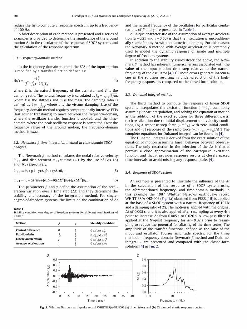
Fig. 1. Whittier Narrows earthquake record WHITTIER/A-ORN006

and the natural frequency of the oscillators for particular combi-nations of b and g are presented in Table 1.

A unique characteristic of the assumption of average accelera-tion (b¼0.25 and g¼0.50) is that the integration is uncondition-ally stable for any Dt with no numerical damping. For this reason,the Newmark b method with average acceleration is commonlyused to model the dynamic response of single and multipledegree of freedom systems.

In addition to the stability issues described above, the New-mark b method has inherent numerical errors associated with thevalue of the input motion time step relative to the naturalfrequency of the oscillator [4,13]. These errors generate inaccura-cies in the solution resulting in under-prediction of the high-frequency response as compared to the closed form solution.

3.3. Duhamel integral method

The third method to compute the response of linear SDOFsystems interpolates the excitation function ð�m €ugÞ, commonlyassuming linear interpolation, and solving the equation of motionas the addition of the exact solution for three different parts:(a) free-vibration due to initial displacement and velocity condi-tions, (b) a response step force ð�m €ugi

Þ with zero initial condi-tions and (c) response of the ramp force ½�mð €ugiþ 1

� €ugiÞ=Dt�. The

complete equations for Duhamel integral can be found in [4].The Duhamel integral is derived from the exact solution of the

equation of motion assuming linear behavior between observa-tions. The only restriction in the selection of the Dt is that itpermits a close approximation of the earthquake excitationfunction and that it provides response results at closely spacedtime intervals to avoid missing any response peaks [4].

3.4. Response of SDOF system

An example is presented to illustrate the influence of the Dt

in the calculation of the response of a SDOF system usingthe aforementioned frequency- and time-domain methods. Inthis example the 1987 Whittier Narrows earthquake recordWHITTIER/A-ORN006 (Fig. 1a) obtained from PEER [16] is appliedat the base of a SDOF system with a natural frequency of 10 Hzand a damping ratio of 2%. The motion is applied with the originalDt of 0.005 s, and it is also applied after resampling at every 4thpoint to increase Dt from 0.005 s to 0.020 s. A low-pass filter isapplied at the Nyquist frequency for Dt¼0.02 s prior to resam-pling to reduce the potential for aliasing of the time series. Theamplitude of the transfer functions, defined as the ratio of theinput and oscillator Fourier amplitude spectra, for the threemethods – frequency-domain, Newmark b method and Duhamelintegral – are presented and compared with the closed-formsolution [4] in Fig. 2.

(a) time history and (b) 5% damped elastic response spectra.

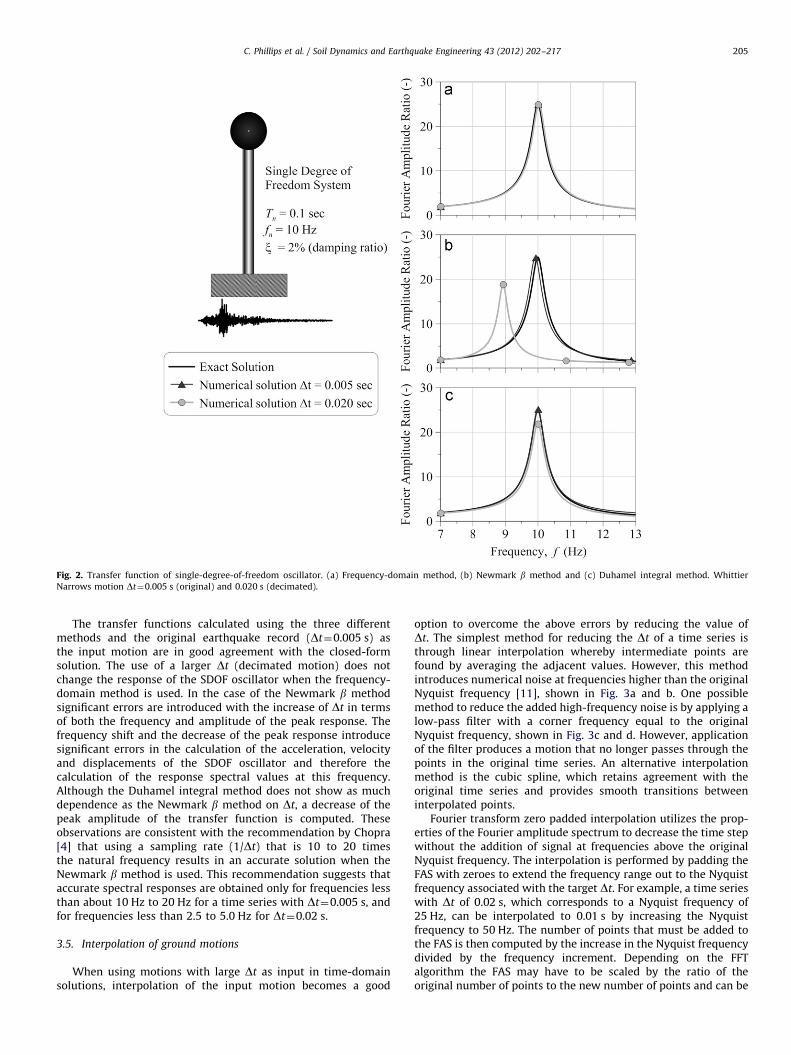
Fig. 2. Transfer function of single-degree-of-freedom oscillator. (a) Frequency-domain method, (b) Newmark b method and (c) Duhamel integral method. Whittier

Narrows motion Dt¼0.005 s (original) and 0.020 s (decimated).


The transfer functions calculated using the three differentmethods and the original earthquake record (Dt¼0.005 s) asthe input motion are in good agreement with the closed-formsolution. The use of a larger Dt (decimated motion) does notchange the response of the SDOF oscillator when the frequency-domain method is used. In the case of the Newmark b methodsignificant errors are introduced with the increase of Dt in termsof both the frequency and amplitude of the peak response. Thefrequency shift and the decrease of the peak response introducesignificant errors in the calculation of the acceleration, velocityand displacements of the SDOF oscillator and therefore thecalculation of the response spectral values at this frequency.Although the Duhamel integral method does not show as muchdependence as the Newmark b method on Dt, a decrease of thepeak amplitude of the transfer function is computed. Theseobservations are consistent with the recommendation by Chopra[4] that using a sampling rate (1/Dt) that is 10 to 20 timesthe natural frequency results in an accurate solution when theNewmark b method is used. This recommendation suggests thataccurate spectral responses are obtained only for frequencies lessthan about 10 Hz to 20 Hz for a time series with Dt¼0.005 s, andfor frequencies less than 2.5 to 5.0 Hz for Dt¼0.02 s.

3.5. Interpolation of ground motions

When using motions with large Dt as input in time-domainsolutions, interpolation of the input motion becomes a good

option to overcome the above errors by reducing the value ofDt. The simplest method for reducing the Dt of a time series isthrough linear interpolation whereby intermediate points arefound by averaging the adjacent values. However, this methodintroduces numerical noise at frequencies higher than the originalNyquist frequency [11], shown in Fig. 3a and b. One possiblemethod to reduce the added high-frequency noise is by applying alow-pass filter with a corner frequency equal to the originalNyquist frequency, shown in Fig. 3c and d. However, applicationof the filter produces a motion that no longer passes through thepoints in the original time series. An alternative interpolationmethod is the cubic spline, which retains agreement with theoriginal time series and provides smooth transitions betweeninterpolated points.

Fourier transform zero padded interpolation utilizes the prop-erties of the Fourier amplitude spectrum to decrease the time stepwithout the addition of signal at frequencies above the originalNyquist frequency. The interpolation is performed by padding theFAS with zeroes to extend the frequency range out to the Nyquistfrequency associated with the target Dt. For example, a time serieswith Dt of 0.02 s, which corresponds to a Nyquist frequency of25 Hz, can be interpolated to 0.01 s by increasing the Nyquistfrequency to 50 Hz. The number of points that must be added tothe FAS is then computed by the increase in the Nyquist frequencydivided by the frequency increment. Depending on the FFTalgorithm the FAS may have to be scaled by the ratio of theoriginal number of points to the new number of points and can be

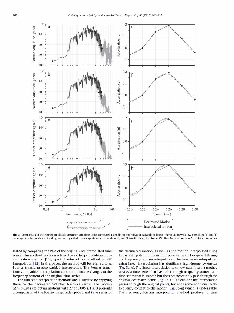
Fig. 3. Comparison of the Fourier amplitude spectrum and time series computed using linear interpolation (a) and (e), linear interpolation with low-pass filter (b) and (f),

cubic spline interpolation (c) and (g) and zero padded Fourier spectrum interpolation (d) and (h) methods applied to the Whittier Narrows motion Dt¼0.02 s time series.


tested by comparing the PGA of the original and interpolated timeseries. This method has been referred to as: frequency-domain re-digitization method [11], spectral interpolation method or FFTinterpolation [12]. In this paper, the method will be referred to asFourier transform zero padded interpolation. The Fourier trans-form zero padded interpolation does not introduce changes to thefrequency content of the original time series.

The different interpolation methods are illustrated by applyingthem to the decimated Whittier Narrows earthquake motion(Dt¼0.020 s) to obtain motions with Dt of 0.005 s. Fig. 3 presentsa comparison of the Fourier amplitude spectra and time series of

the decimated motion, as well as the motion interpolated usinglinear interpolation, linear interpolation with low-pass filtering,and frequency-domain interpolation. The time series interpolatedusing linear interpolation has significant high-frequency energy(Fig. 3a–e). The linear interpolation with low-pass filtering methodcreates a time series that has reduced high-frequency content andtime series that is smooth but does not necessarily pass through theoriginal, decimated points (Fig. 3b–f). The cubic spline interpolationpasses through the original points, but adds some additional high-frequency content to the motion (Fig. 3c–g) which is undesirable.The frequency-domain interpolation method produces a time


series that is smooth, similar to the time series obtained withlinear interpolation and low-pass filtering, but does so withoutany change in the frequency content (Fig. 3d–g). The cubic splineand the frequency-domain interpolation methods provide almostthe same time series, however as it has already been highlightedthe use of cubic spline interpolation even when a low-pass filter isused introduces undesirable high-frequency content.

Time domain solutions such as the Newmark b and Duhamelintegral methods typically use linear interpolation to increase thenumber of steps and decrease Dt to improve the accuracy of thesolution. Linear interpolation is commonly used in time-domainsolutions for its simplicity. In the case of frequency domainsolutions, such as the one presented for SDOF systems, thecalculation of the FAS is required and therefore the implementa-tion of the frequency domain, Fourier transform zero paddedinterpolation method is commonly used as it is straightforwardand does not introduce additional complexity to the solution.

3.6. Response spectra comparison

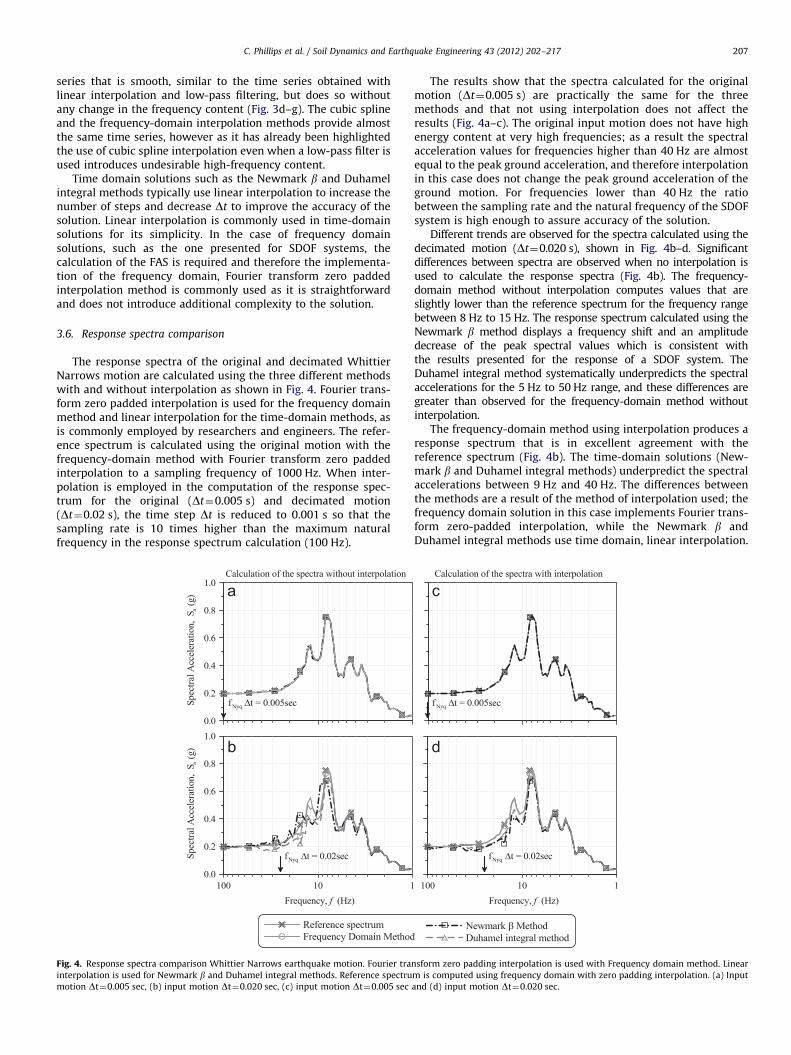
The response spectra of the original and decimated WhittierNarrows motion are calculated using the three different methodswith and without interpolation as shown in Fig. 4. Fourier trans-form zero padded interpolation is used for the frequency domainmethod and linear interpolation for the time-domain methods, asis commonly employed by researchers and engineers. The refer-ence spectrum is calculated using the original motion with thefrequency-domain method with Fourier transform zero paddedinterpolation to a sampling frequency of 1000 Hz. When inter-polation is employed in the computation of the response spec-trum for the original (Dt¼0.005 s) and decimated motion(Dt¼0.02 s), the time step Dt is reduced to 0.001 s so that thesampling rate is 10 times higher than the maximum naturalfrequency in the response spectrum calculation (100 Hz).

Fig. 4. Response spectra comparison Whittier Narrows earthquake motion. Fourier tra

interpolation is used for Newmark b and Duhamel integral methods. Reference spectru

motion Dt¼0.005 sec, (b) input motion Dt¼0.020 sec, (c) input motion Dt¼0.005 sec

The results show that the spectra calculated for the originalmotion (Dt¼0.005 s) are practically the same for the threemethods and that not using interpolation does not affect theresults (Fig. 4a–c). The original input motion does not have highenergy content at very high frequencies; as a result the spectralacceleration values for frequencies higher than 40 Hz are almostequal to the peak ground acceleration, and therefore interpolationin this case does not change the peak ground acceleration of theground motion. For frequencies lower than 40 Hz the ratiobetween the sampling rate and the natural frequency of the SDOFsystem is high enough to assure accuracy of the solution.

Different trends are observed for the spectra calculated using thedecimated motion (Dt¼0.020 s), shown in Fig. 4b–d. Significantdifferences between spectra are observed when no interpolation isused to calculate the response spectra (Fig. 4b). The frequency-domain method without interpolation computes values that areslightly lower than the reference spectrum for the frequency rangebetween 8 Hz to 15 Hz. The response spectrum calculated using theNewmark b method displays a frequency shift and an amplitudedecrease of the peak spectral values which is consistent withthe results presented for the response of a SDOF system. TheDuhamel integral method systematically underpredicts the spectralaccelerations for the 5 Hz to 50 Hz range, and these differences aregreater than observed for the frequency-domain method withoutinterpolation.

The frequency-domain method using interpolation produces aresponse spectrum that is in excellent agreement with thereference spectrum (Fig. 4b). The time-domain solutions (New-mark b and Duhamel integral methods) underpredict the spectralaccelerations between 9 Hz and 40 Hz. The differences betweenthe methods are a result of the method of interpolation used; thefrequency domain solution in this case implements Fourier trans-form zero-padded interpolation, while the Newmark b andDuhamel integral methods use time domain, linear interpolation.

nsform zero padding interpolation is used with Frequency domain method. Linear

m is computed using frequency domain with zero padding interpolation. (a) Input

and (d) input motion Dt¼0.020 sec.


As evidenced in Fig. 3, Fourier transform zero-padded interpola-tion produces ground motions with higher peak accelerationvalues than the linear interpolation method. Response spectraare calculated for 16 earthquake ground motions obtainedfrom PEER [16], listed in Table 2, to consider motion variability inevaluating Dt effects. For each of the ground motions, the originaltime series with Dt of 0.005 s is low-pass filtered at the new Nyquistfrequency to reduce the aliasing effects and then decimated to Dt of0.020 s. The response spectrum is calculated for the full set of motionsusing the different methods of response spectrum calculation andinterpolation described in this paper. In order to gain a betterunderstanding of the differences due to a change in the time stepof a ground motion, the relative difference between a spectralacceleration (Sa) and a reference spectral acceleration (Sa,ref) is definedas the relative spectral acceleration difference [Eq. (7)]:

dSa ¼Sa�Sa,ref

Sa,refð7Þ

where Sa,ref is the reference spectral acceleration computed using theoriginal ground motion (Dt¼0.005 s) with the frequency-domainmethod and Fourier transform zero padded interpolation to 1000 Hz.

Table 2Earthquakes seismic records used in equivalent-linear or non-linear 1D site

response. Ground motions were obtained from PEER database (2010).

Earthquake Record name Date PGA (g) Recorded

Dt (s)

Anza ANZA/RDA045 02/25/80 0.097 0.005

Chalfant Valley CHALFANT/

A-BPL070

07/21/86 0.165 0.005

Chi–Chi CHICHI/ALS-E 09/20/99 0.183 0.005

Coalinga COALINGA/

A-SGT080

05/09/83 0.244 0.005

Coyote Lake COYOTELK/

G01230

08/06/79 0.132 0.005

Hollister HOLLISTR/

A-G01157

11/28/74 0.132 0.005

Imperial IMPVALL/

H-SUP045

10/15/79 0.195 0.005

Kocaeli KOCAELI/GBZ000 08/17/99 0.244 0.005

Landers LANDERS/MVH000 6/28/92 0.188 0.005

Loma Prieta LOMAP/FRE000 10/18/89 0.124 0.005

Mammoth Lakes MAMMOTH/

I-LUL000

05/25/80 0.194 0.005

Morgan Hill MORGAN/G06000 04/24/84 0.222 0.005

Palm Springs PALMSPR/CFR225 07/08/86 0.169 0.005

Nahanni NAHANNI/S3270 12/23/85 0.148 0.005

San Fernando SFERN/FSD172 02/09/71 0.152 0.005

WhittierNarrows

WHITTIER/

A-ORN006

10/01/87 0.198 0.005

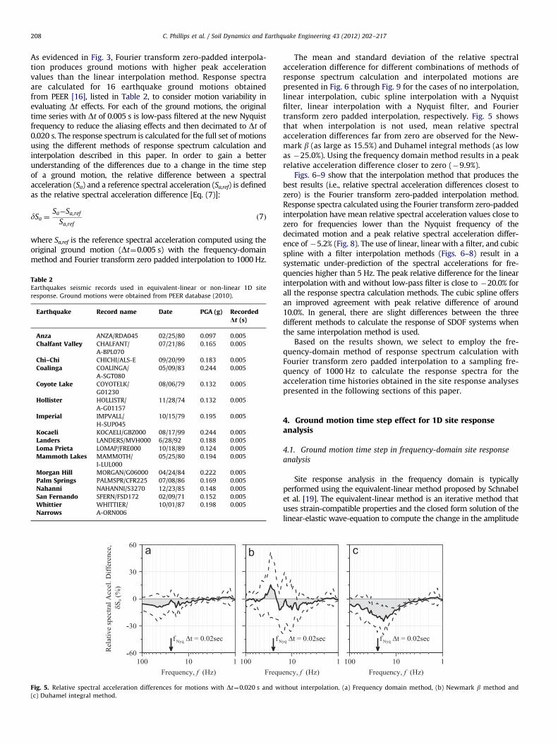
Fig. 5. Relative spectral acceleration differences for motions with Dt¼0.020 s and w

(c) Duhamel integral method.

The mean and standard deviation of the relative spectralacceleration difference for different combinations of methods ofresponse spectrum calculation and interpolated motions arepresented in Fig. 6 through Fig. 9 for the cases of no interpolation,linear interpolation, cubic spline interpolation with a Nyquistfilter, linear interpolation with a Nyquist filter, and Fouriertransform zero padded interpolation, respectively. Fig. 5 showsthat when interpolation is not used, mean relative spectralacceleration differences far from zero are observed for the New-mark b (as large as 15.5%) and Duhamel integral methods (as lowas �25.0%). Using the frequency domain method results in a peakrelative acceleration difference closer to zero (�9.9%).

Figs. 6–9 show that the interpolation method that produces thebest results (i.e., relative spectral acceleration differences closest tozero) is the Fourier transform zero-padded interpolation method.Response spectra calculated using the Fourier transform zero-paddedinterpolation have mean relative spectral acceleration values close tozero for frequencies lower than the Nyquist frequency of thedecimated motion and a peak relative spectral acceleration differ-ence of �5.2% (Fig. 8). The use of linear, linear with a filter, and cubicspline with a filter interpolation methods (Figs. 6–8) result in asystematic under-prediction of the spectral accelerations for fre-quencies higher than 5 Hz. The peak relative difference for the linearinterpolation with and without low-pass filter is close to �20.0% forall the response spectra calculation methods. The cubic spline offersan improved agreement with peak relative difference of around10.0%. In general, there are slight differences between the threedifferent methods to calculate the response of SDOF systems whenthe same interpolation method is used.

Based on the results shown, we select to employ the fre-quency-domain method of response spectrum calculation withFourier transform zero padded interpolation to a sampling fre-quency of 1000 Hz to calculate the response spectra for theacceleration time histories obtained in the site response analysespresented in the following sections of this paper.

4. Ground motion time step effect for 1D site responseanalysis

4.1. Ground motion time step in frequency-domain site response

analysis

Site response analysis in the frequency domain is typicallyperformed using the equivalent-linear method proposed by Schnabelet al. [19]. The equivalent-linear method is an iterative method thatuses strain-compatible properties and the closed form solution of thelinear-elastic wave-equation to compute the change in the amplitude

ithout interpolation. (a) Frequency domain method, (b) Newmark b method and

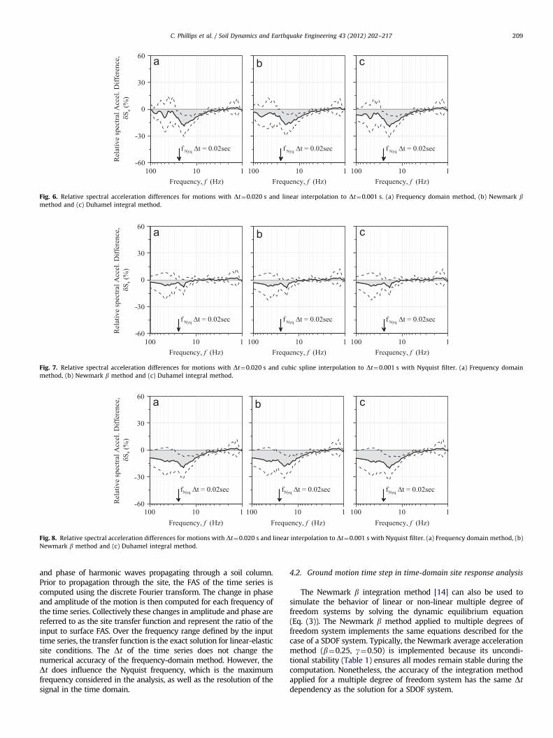
Fig. 8. Relative spectral acceleration differences for motions with Dt¼0.020 s and linear interpolation to Dt¼0.001 s with Nyquist filter. (a) Frequency domain method, (b)

Newmark b method and (c) Duhamel integral method.

Fig. 7. Relative spectral acceleration differences for motions with Dt¼0.020 s and cubic spline interpolation to Dt¼0.001 s with Nyquist filter. (a) Frequency domain

method, (b) Newmark b method and (c) Duhamel integral method.

Fig. 6. Relative spectral acceleration differences for motions with Dt¼0.020 s and linear interpolation to Dt¼0.001 s. (a) Frequency domain method, (b) Newmark bmethod and (c) Duhamel integral method.


and phase of harmonic waves propagating through a soil column.Prior to propagation through the site, the FAS of the time series iscomputed using the discrete Fourier transform. The change in phaseand amplitude of the motion is then computed for each frequency ofthe time series. Collectively these changes in amplitude and phase arereferred to as the site transfer function and represent the ratio of theinput to surface FAS. Over the frequency range defined by the inputtime series, the transfer function is the exact solution for linear-elasticsite conditions. The Dt of the time series does not change thenumerical accuracy of the frequency-domain method. However, theDt does influence the Nyquist frequency, which is the maximumfrequency considered in the analysis, as well as the resolution of thesignal in the time domain.

4.2. Ground motion time step in time-domain site response analysis

The Newmark b integration method [14] can also be used tosimulate the behavior of linear or non-linear multiple degree offreedom systems by solving the dynamic equilibrium equation(Eq. (3)). The Newmark b method applied to multiple degrees offreedom system implements the same equations described for thecase of a SDOF system. Typically, the Newmark average accelerationmethod (b¼0.25, g¼0.50) is implemented because its uncondi-tional stability (Table 1) ensures all modes remain stable during thecomputation. Nonetheless, the accuracy of the integration methodapplied for a multiple degree of freedom system has the same Dt

dependency as the solution for a SDOF system.

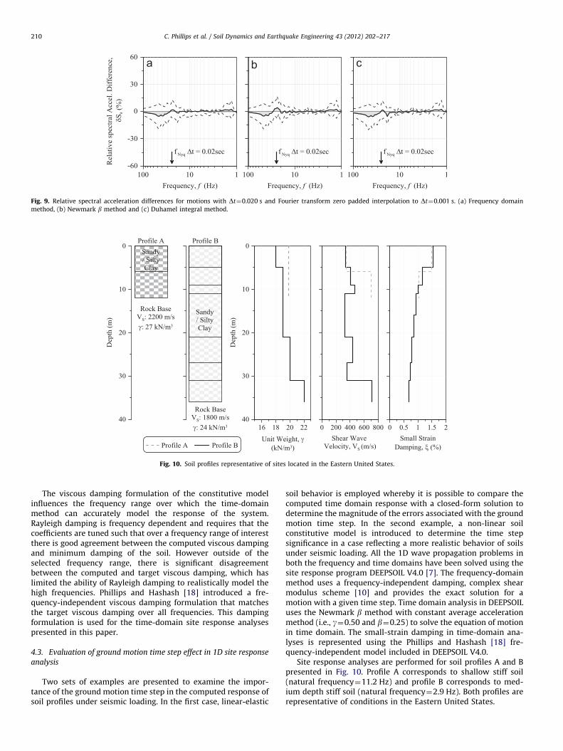
Fig. 10. Soil profiles representative of sites located in the Eastern United States.

Fig. 9. Relative spectral acceleration differences for motions with Dt¼0.020 s and Fourier transform zero padded interpolation to Dt¼0.001 s. (a) Frequency domain

method, (b) Newmark b method and (c) Duhamel integral method.


The viscous damping formulation of the constitutive modelinfluences the frequency range over which the time-domainmethod can accurately model the response of the system.Rayleigh damping is frequency dependent and requires that thecoefficients are tuned such that over a frequency range of interestthere is good agreement between the computed viscous dampingand minimum damping of the soil. However outside of theselected frequency range, there is significant disagreementbetween the computed and target viscous damping, which haslimited the ability of Rayleigh damping to realistically model thehigh frequencies. Phillips and Hashash [18] introduced a fre-quency-independent viscous damping formulation that matchesthe target viscous damping over all frequencies. This dampingformulation is used for the time-domain site response analysespresented in this paper.

4.3. Evaluation of ground motion time step effect in 1D site response

analysis

Two sets of examples are presented to examine the impor-tance of the ground motion time step in the computed response ofsoil profiles under seismic loading. In the first case, linear-elastic

soil behavior is employed whereby it is possible to compare thecomputed time domain response with a closed-form solution todetermine the magnitude of the errors associated with the groundmotion time step. In the second example, a non-linear soilconstitutive model is introduced to determine the time stepsignificance in a case reflecting a more realistic behavior of soilsunder seismic loading. All the 1D wave propagation problems inboth the frequency and time domains have been solved using thesite response program DEEPSOIL V4.0 [7]. The frequency-domainmethod uses a frequency-independent damping, complex shearmodulus scheme [10] and provides the exact solution for amotion with a given time step. Time domain analysis in DEEPSOILuses the Newmark b method with constant average accelerationmethod (i.e., g¼0.50 and b¼0.25) to solve the equation of motionin time domain. The small-strain damping in time-domain ana-lyses is represented using the Phillips and Hashash [18] fre-quency-independent model included in DEEPSOIL V4.0.

Site response analyses are performed for soil profiles A and Bpresented in Fig. 10. Profile A corresponds to shallow stiff soil(natural frequency¼11.2 Hz) and profile B corresponds to med-ium depth stiff soil (natural frequency¼2.9 Hz). Both profiles arerepresentative of conditions in the Eastern United States.


The ground motion time series used in these examples are theoriginal ground motions with Dt¼0.005 s listed in Table 2 and thedecimated motions with Dt¼0.020 s, previously used for theresponse spectra analyses.

4.3.1. Case 1: linear-elastic soil constitutive behavior with viscous

damping

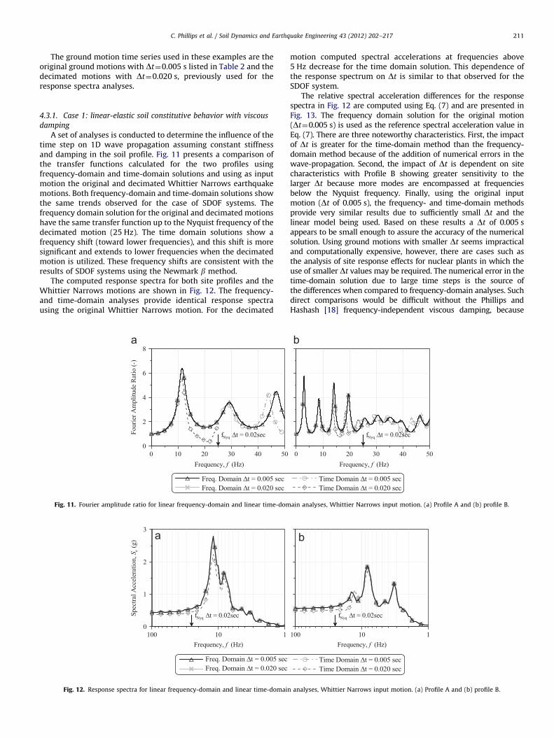
A set of analyses is conducted to determine the influence of thetime step on 1D wave propagation assuming constant stiffnessand damping in the soil profile. Fig. 11 presents a comparison ofthe transfer functions calculated for the two profiles usingfrequency-domain and time-domain solutions and using as inputmotion the original and decimated Whittier Narrows earthquakemotions. Both frequency-domain and time-domain solutions showthe same trends observed for the case of SDOF systems. Thefrequency domain solution for the original and decimated motionshave the same transfer function up to the Nyquist frequency of thedecimated motion (25 Hz). The time domain solutions show afrequency shift (toward lower frequencies), and this shift is moresignificant and extends to lower frequencies when the decimatedmotion is utilized. These frequency shifts are consistent with theresults of SDOF systems using the Newmark b method.

The computed response spectra for both site profiles and theWhittier Narrows motions are shown in Fig. 12. The frequency-and time-domain analyses provide identical response spectrausing the original Whittier Narrows motion. For the decimated

Fig. 11. Fourier amplitude ratio for linear frequency-domain and linear time-dom

Fig. 12. Response spectra for linear frequency-domain and linear time-domain

motion computed spectral accelerations at frequencies above5 Hz decrease for the time domain solution. This dependence ofthe response spectrum on Dt is similar to that observed for theSDOF system.

The relative spectral acceleration differences for the responsespectra in Fig. 12 are computed using Eq. (7) and are presented inFig. 13. The frequency domain solution for the original motion(Dt¼0.005 s) is used as the reference spectral acceleration value inEq. (7). There are three noteworthy characteristics. First, the impactof Dt is greater for the time-domain method than the frequency-domain method because of the addition of numerical errors in thewave-propagation. Second, the impact of Dt is dependent on sitecharacteristics with Profile B showing greater sensitivity to thelarger Dt because more modes are encompassed at frequenciesbelow the Nyquist frequency. Finally, using the original inputmotion (Dt of 0.005 s), the frequency- and time-domain methodsprovide very similar results due to sufficiently small Dt and thelinear model being used. Based on these results a Dt of 0.005 sappears to be small enough to assure the accuracy of the numericalsolution. Using ground motions with smaller Dt seems impracticaland computationally expensive, however, there are cases such asthe analysis of site response effects for nuclear plants in which theuse of smaller Dt values may be required. The numerical error in thetime-domain solution due to large time steps is the source ofthe differences when compared to frequency-domain analyses. Suchdirect comparisons would be difficult without the Phillips andHashash [18] frequency-independent viscous damping, because

ain analyses, Whittier Narrows input motion. (a) Profile A and (b) profile B.

analyses, Whittier Narrows input motion. (a) Profile A and (b) profile B.

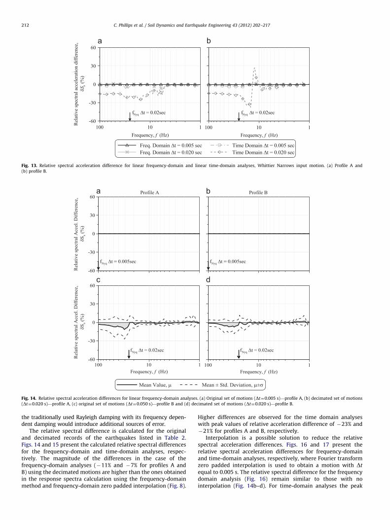
Fig. 13. Relative spectral acceleration difference for linear frequency-domain and linear time-domain analyses, Whittier Narrows input motion. (a) Profile A and

(b) profile B.

Fig. 14. Relative spectral acceleration differences for linear frequency-domain analyses. (a) Original set of motions (Dt¼0.005 s)—profile A, (b) decimated set of motions

(Dt¼0.020 s)—profile A, (c) original set of motions (Dt¼0.050 s)—profile B and (d) decimated set of motions (Dt¼0.020 s)—profile B.


the traditionally used Rayleigh damping with its frequency depen-dent damping would introduce additional sources of error.

The relative spectral difference is calculated for the originaland decimated records of the earthquakes listed in Table 2.Figs. 14 and 15 present the calculated relative spectral differencesfor the frequency-domain and time-domain analyses, respec-tively. The magnitude of the differences in the case of thefrequency-domain analyses (�11% and �7% for profiles A andB) using the decimated motions are higher than the ones obtainedin the response spectra calculation using the frequency-domainmethod and frequency-domain zero padded interpolation (Fig. 8).

Higher differences are observed for the time domain analyseswith peak values of relative acceleration difference of �23% and�21% for profiles A and B, respectively.

Interpolation is a possible solution to reduce the relativespectral acceleration differences. Figs. 16 and 17 present therelative spectral acceleration differences for frequency-domainand time-domain analyses, respectively, where Fourier transformzero padded interpolation is used to obtain a motion with Dt

equal to 0.005 s. The relative spectral difference for the frequencydomain analysis (Fig. 16) remain similar to those with nointerpolation (Fig. 14b–d). For time-domain analyses the peak

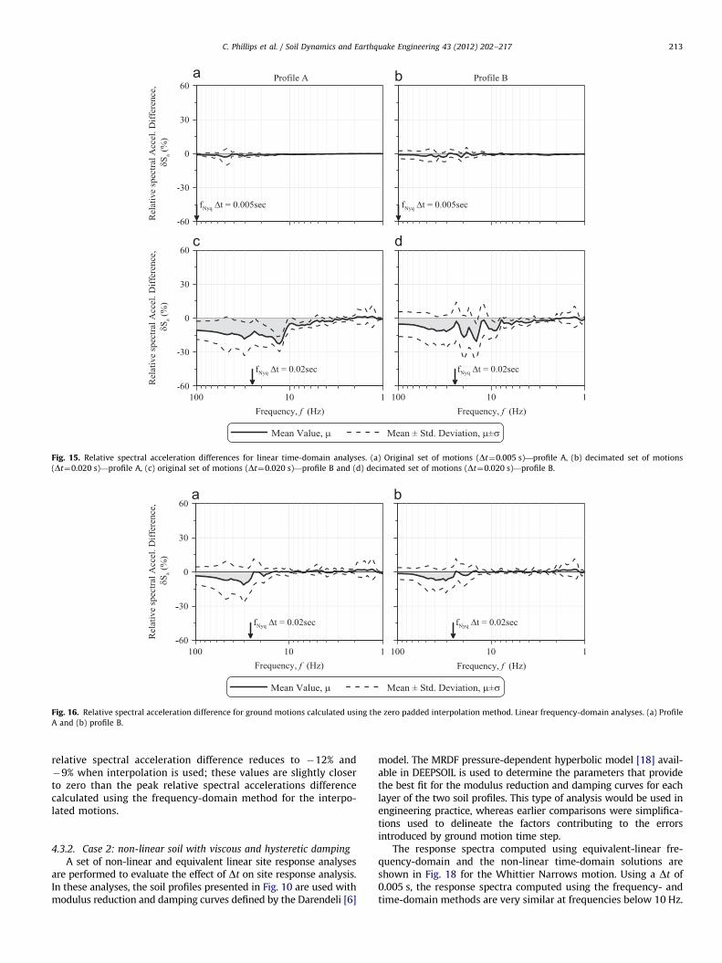
Fig. 15. Relative spectral acceleration differences for linear time-domain analyses. (a) Original set of motions (Dt¼0.005 s)—profile A, (b) decimated set of motions

(Dt¼0.020 s)—profile A, (c) original set of motions (Dt¼0.020 s)—profile B and (d) decimated set of motions (Dt¼0.020 s)—profile B.

Fig. 16. Relative spectral acceleration difference for ground motions calculated using the zero padded interpolation method. Linear frequency-domain analyses. (a) Profile

A and (b) profile B.


relative spectral acceleration difference reduces to �12% and�9% when interpolation is used; these values are slightly closerto zero than the peak relative spectral accelerations differencecalculated using the frequency-domain method for the interpo-lated motions.

4.3.2. Case 2: non-linear soil with viscous and hysteretic damping

A set of non-linear and equivalent linear site response analysesare performed to evaluate the effect of Dt on site response analysis.In these analyses, the soil profiles presented in Fig. 10 are used withmodulus reduction and damping curves defined by the Darendeli [6]

model. The MRDF pressure-dependent hyperbolic model [18] avail-able in DEEPSOIL is used to determine the parameters that providethe best fit for the modulus reduction and damping curves for eachlayer of the two soil profiles. This type of analysis would be used inengineering practice, whereas earlier comparisons were simplifica-tions used to delineate the factors contributing to the errorsintroduced by ground motion time step.

The response spectra computed using equivalent-linear fre-quency-domain and the non-linear time-domain solutions areshown in Fig. 18 for the Whittier Narrows motion. Using a Dt of0.005 s, the response spectra computed using the frequency- andtime-domain methods are very similar at frequencies below 10 Hz.

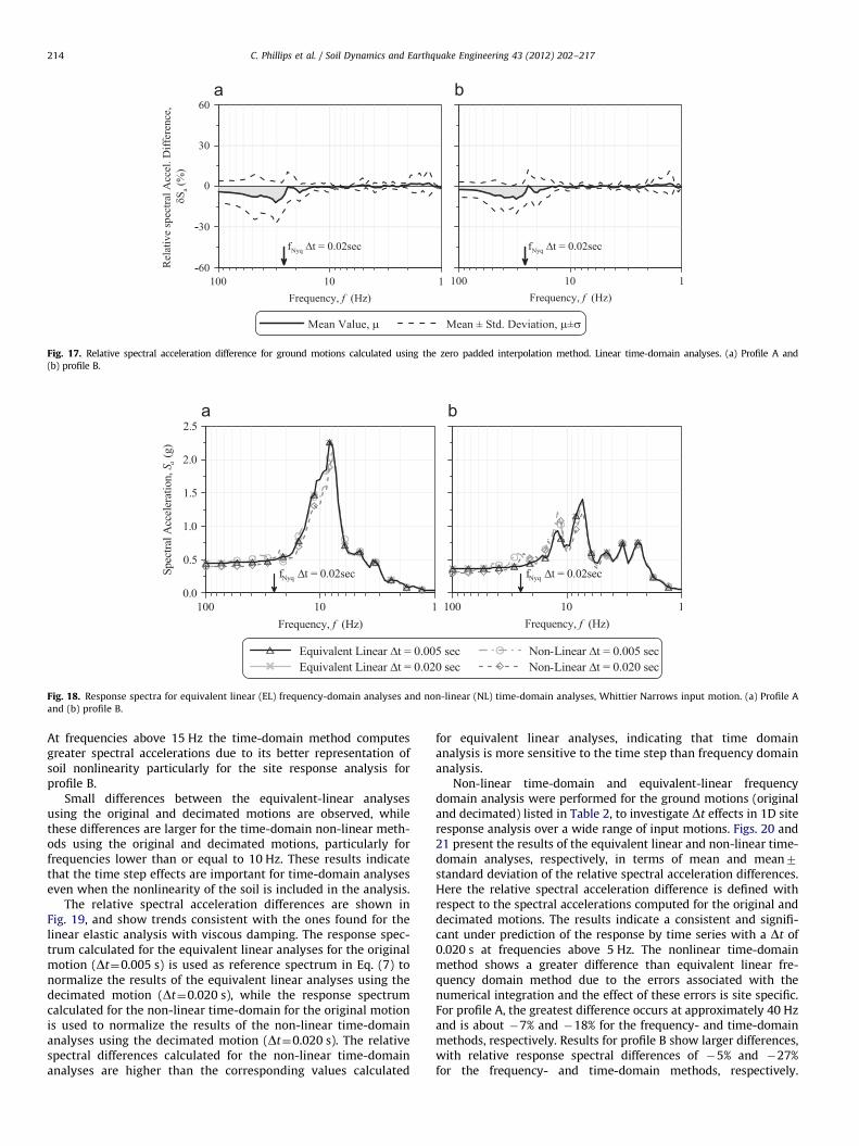
Fig. 17. Relative spectral acceleration difference for ground motions calculated using the zero padded interpolation method. Linear time-domain analyses. (a) Profile A and

(b) profile B.

Fig. 18. Response spectra for equivalent linear (EL) frequency-domain analyses and non-linear (NL) time-domain analyses, Whittier Narrows input motion. (a) Profile A

and (b) profile B.


At frequencies above 15 Hz the time-domain method computesgreater spectral accelerations due to its better representation ofsoil nonlinearity particularly for the site response analysis forprofile B.

Small differences between the equivalent-linear analysesusing the original and decimated motions are observed, whilethese differences are larger for the time-domain non-linear meth-ods using the original and decimated motions, particularly forfrequencies lower than or equal to 10 Hz. These results indicatethat the time step effects are important for time-domain analyseseven when the nonlinearity of the soil is included in the analysis.

The relative spectral acceleration differences are shown inFig. 19, and show trends consistent with the ones found for thelinear elastic analysis with viscous damping. The response spec-trum calculated for the equivalent linear analyses for the originalmotion (Dt¼0.005 s) is used as reference spectrum in Eq. (7) tonormalize the results of the equivalent linear analyses using thedecimated motion (Dt¼0.020 s), while the response spectrumcalculated for the non-linear time-domain for the original motionis used to normalize the results of the non-linear time-domainanalyses using the decimated motion (Dt¼0.020 s). The relativespectral differences calculated for the non-linear time-domainanalyses are higher than the corresponding values calculated

for equivalent linear analyses, indicating that time domainanalysis is more sensitive to the time step than frequency domainanalysis.

Non-linear time-domain and equivalent-linear frequencydomain analysis were performed for the ground motions (originaland decimated) listed in Table 2, to investigate Dt effects in 1D siteresponse analysis over a wide range of input motions. Figs. 20 and21 present the results of the equivalent linear and non-linear time-domain analyses, respectively, in terms of mean and mean7standard deviation of the relative spectral acceleration differences.Here the relative spectral acceleration difference is defined withrespect to the spectral accelerations computed for the original anddecimated motions. The results indicate a consistent and signifi-cant under prediction of the response by time series with a Dt of0.020 s at frequencies above 5 Hz. The nonlinear time-domainmethod shows a greater difference than equivalent linear fre-quency domain method due to the errors associated with thenumerical integration and the effect of these errors is site specific.For profile A, the greatest difference occurs at approximately 40 Hzand is about �7% and �18% for the frequency- and time-domainmethods, respectively. Results for profile B show larger differences,with relative response spectral differences of �5% and �27%for the frequency- and time-domain methods, respectively.

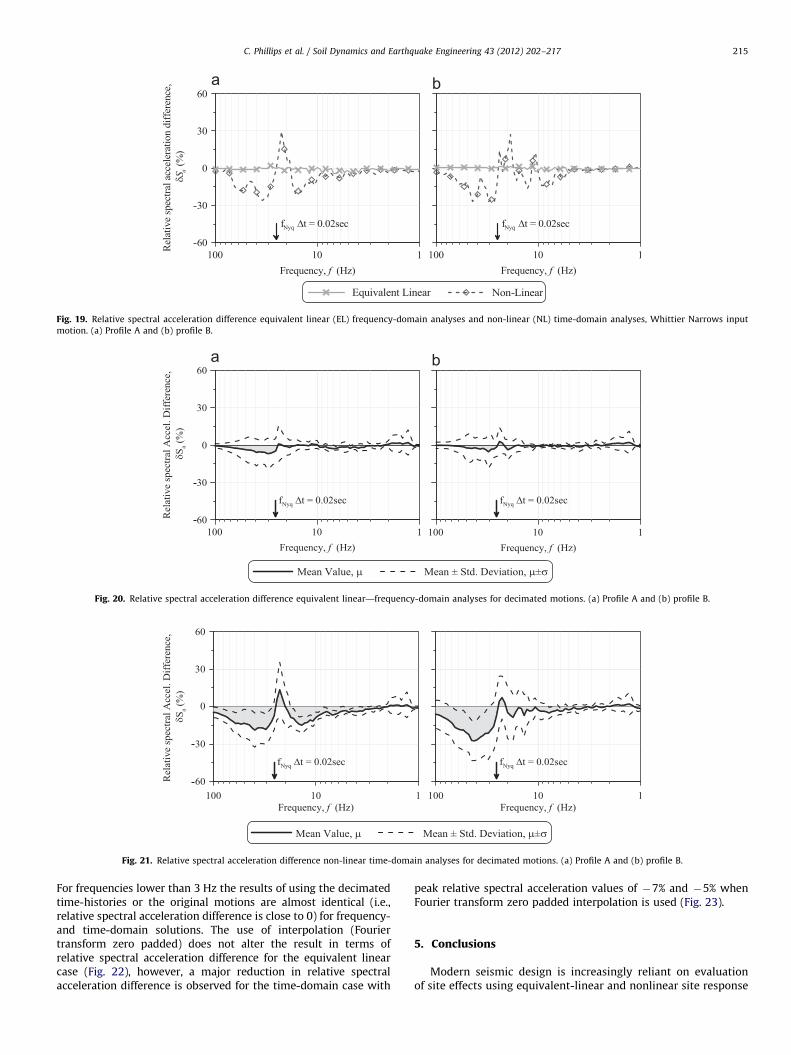
Fig. 19. Relative spectral acceleration difference equivalent linear (EL) frequency-domain analyses and non-linear (NL) time-domain analyses, Whittier Narrows input

motion. (a) Profile A and (b) profile B.

Fig. 20. Relative spectral acceleration difference equivalent linear—frequency-domain analyses for decimated motions. (a) Profile A and (b) profile B.

Fig. 21. Relative spectral acceleration difference non-linear time-domain analyses for decimated motions. (a) Profile A and (b) profile B.


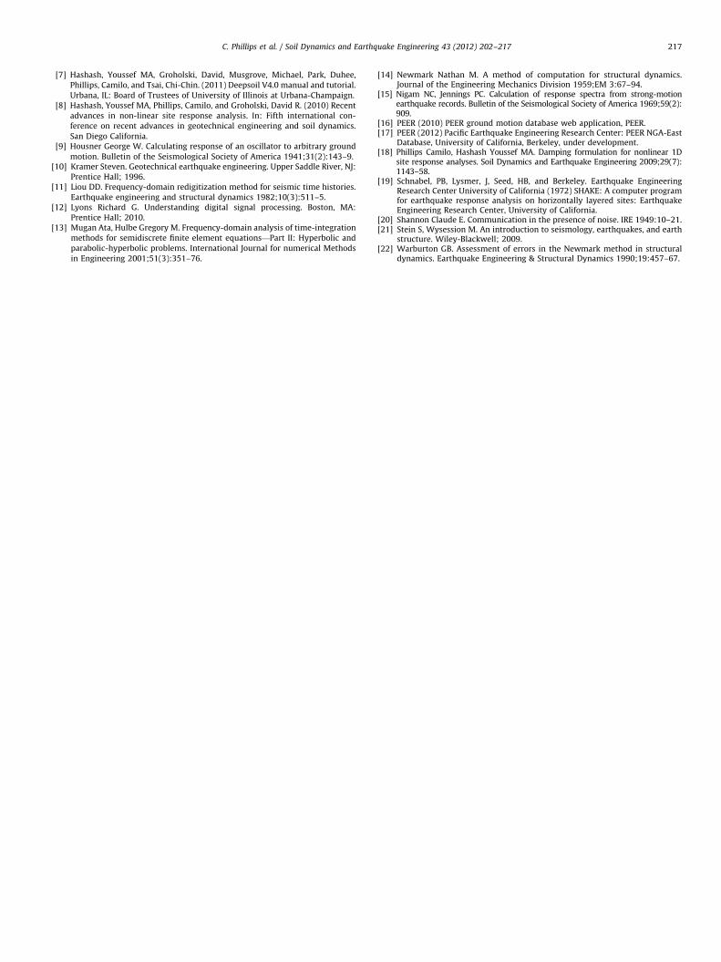
For frequencies lower than 3 Hz the results of using the decimatedtime-histories or the original motions are almost identical (i.e.,relative spectral acceleration difference is close to 0) for frequency-and time-domain solutions. The use of interpolation (Fouriertransform zero padded) does not alter the result in terms ofrelative spectral acceleration difference for the equivalent linearcase (Fig. 22), however, a major reduction in relative spectralacceleration difference is observed for the time-domain case with

peak relative spectral acceleration values of �7% and �5% whenFourier transform zero padded interpolation is used (Fig. 23).

5. Conclusions

Modern seismic design is increasingly reliant on evaluationof site effects using equivalent-linear and nonlinear site response

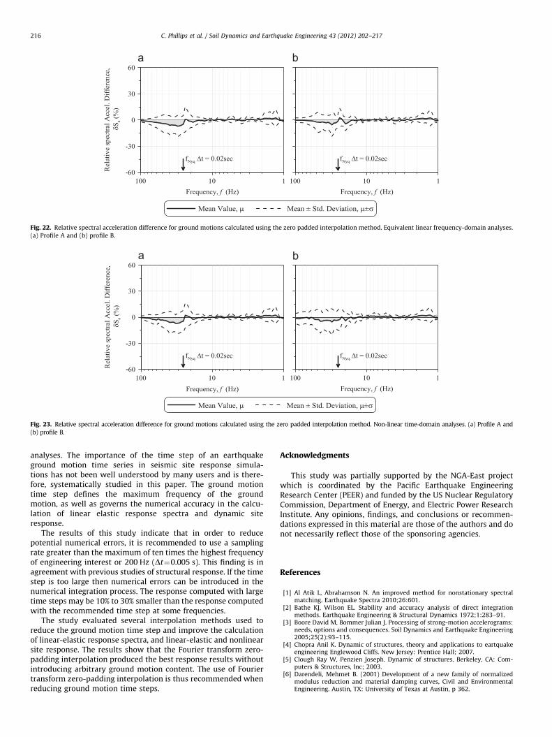
Fig. 22. Relative spectral acceleration difference for ground motions calculated using the zero padded interpolation method. Equivalent linear frequency-domain analyses.

(a) Profile A and (b) profile B.

Fig. 23. Relative spectral acceleration difference for ground motions calculated using the zero padded interpolation method. Non-linear time-domain analyses. (a) Profile A and

(b) profile B.


analyses. The importance of the time step of an earthquakeground motion time series in seismic site response simula-tions has not been well understood by many users and is there-fore, systematically studied in this paper. The ground motiontime step defines the maximum frequency of the groundmotion, as well as governs the numerical accuracy in the calcu-lation of linear elastic response spectra and dynamic siteresponse.

The results of this study indicate that in order to reducepotential numerical errors, it is recommended to use a samplingrate greater than the maximum of ten times the highest frequencyof engineering interest or 200 Hz (Dt¼0.005 s). This finding is inagreement with previous studies of structural response. If the timestep is too large then numerical errors can be introduced in thenumerical integration process. The response computed with largetime steps may be 10% to 30% smaller than the response computedwith the recommended time step at some frequencies.

The study evaluated several interpolation methods used toreduce the ground motion time step and improve the calculationof linear-elastic response spectra, and linear-elastic and nonlinearsite response. The results show that the Fourier transform zero-padding interpolation produced the best response results withoutintroducing arbitrary ground motion content. The use of Fouriertransform zero-padding interpolation is thus recommended whenreducing ground motion time steps.

Acknowledgments

This study was partially supported by the NGA-East projectwhich is coordinated by the Pacific Earthquake EngineeringResearch Center (PEER) and funded by the US Nuclear RegulatoryCommission, Department of Energy, and Electric Power ResearchInstitute. Any opinions, findings, and conclusions or recommen-dations expressed in this material are those of the authors and donot necessarily reflect those of the sponsoring agencies.

References

[1] Al Atik L, Abrahamson N. An improved method for nonstationary spectralmatching. Earthquake Spectra 2010;26:601.

[2] Bathe KJ, Wilson EL. Stability and accuracy analysis of direct integrationmethods. Earthquake Engineering & Structural Dynamics 1972;1:283–91.

[3] Boore David M, Bommer Julian J. Processing of strong-motion accelerograms:needs, options and consequences. Soil Dynamics and Earthquake Engineering2005;25(2):93–115.

[4] Chopra Anil K. Dynamic of structures, theory and applications to eartquakeengineering Englewood Cliffs. New Jersey: Prentice Hall; 2007.

[5] Clough Ray W, Penzien Joseph. Dynamic of structures. Berkeley, CA: Com-puters & Structures, Inc; 2003.

[6] Darendeli, Mehmet B. (2001) Development of a new family of normalizedmodulus reduction and material damping curves, Civil and EnvironmentalEngineering. Austin, TX: University of Texas at Austin, p 362.


[7] Hashash, Youssef MA, Groholski, David, Musgrove, Michael, Park, Duhee,Phillips, Camilo, and Tsai, Chi-Chin. (2011) Deepsoil V4.0 manual and tutorial.Urbana, IL: Board of Trustees of University of Illinois at Urbana-Champaign.

[8] Hashash, Youssef MA, Phillips, Camilo, and Groholski, David R. (2010) Recentadvances in non-linear site response analysis. In: Fifth international con-ference on recent advances in geotechnical engineering and soil dynamics.

San Diego California.[9] Housner George W. Calculating response of an oscillator to arbitrary ground

motion. Bulletin of the Seismological Society of America 1941;31(2):143–9.[10] Kramer Steven. Geotechnical earthquake engineering. Upper Saddle River, NJ:

Prentice Hall; 1996.[11] Liou DD. Frequency-domain redigitization method for seismic time histories.

Earthquake engineering and structural dynamics 1982;10(3):511–5.[12] Lyons Richard G. Understanding digital signal processing. Boston, MA:

Prentice Hall; 2010.[13] Mugan Ata, Hulbe Gregory M. Frequency-domain analysis of time-integration

methods for semidiscrete finite element equations—Part II: Hyperbolic andparabolic-hyperbolic problems. International Journal for numerical Methods

in Engineering 2001;51(3):351–76.

[14] Newmark Nathan M. A method of computation for structural dynamics.Journal of the Engineering Mechanics Division 1959;EM 3:67–94.

[15] Nigam NC, Jennings PC. Calculation of response spectra from strong-motionearthquake records. Bulletin of the Seismological Society of America 1969;59(2):909.

[16] PEER (2010) PEER ground motion database web application, PEER.[17] PEER (2012) Pacific Earthquake Engineering Research Center: PEER NGA-East

Database, University of California, Berkeley, under development.[18] Phillips Camilo, Hashash Youssef MA. Damping formulation for nonlinear 1D

site response analyses. Soil Dynamics and Earthquake Engineering 2009;29(7):1143–58.

[19] Schnabel, PB, Lysmer, J, Seed, HB, and Berkeley. Earthquake EngineeringResearch Center University of California (1972) SHAKE: A computer programfor earthquake response analysis on horizontally layered sites: EarthquakeEngineering Research Center, University of California.

[20] Shannon Claude E. Communication in the presence of noise. IRE 1949:10–21.[21] Stein S, Wysession M. An introduction to seismology, earthquakes, and earth

structure. Wiley-Blackwell; 2009.[22] Warburton GB. Assessment of errors in the Newmark method in structural

dynamics. Earthquake Engineering & Structural Dynamics 1990;19:457–67.

Documents

Significance of ground motion time step in one dimensional site response analysis