Signatures of ExtraDimensions

Coen Boellaard, Kris Holsheimer, Rose Koopman, Philipp Moser and Ido Niesen

June 29, 2005

Abstract

The possible effects of extra spatial dimensions as described in theADD model might be detectable in future colliders such as the LHC atCERN. This article reviews two detectable consequences of these extraspatial dimensions at high energy collisions: black hole production andmissing energy. Also included is a theoretical background about bothcompactified extra spatial dimensions and Kaluza Klein reduction in orderto give the reader some insight in the concept of extra spatial dimensions.

Contents

1 Theory 31.1 Introduction . . . . . . . . . . . . . . . . . . . . . . . . . . . . . . 31.2 Kaluza-Klein Reduction . . . . . . . . . . . . . . . . . . . . . . . 41.3 The Hierarchy Problem . . . . . . . . . . . . . . . . . . . . . . . 5

1.3.1 Higher Dimensional Gravity . . . . . . . . . . . . . . . . . 51.3.2 The ADD Model . . . . . . . . . . . . . . . . . . . . . . . 10

2 Missing Energy 122.1 Interdimensional gravitons . . . . . . . . . . . . . . . . . . . . . . 122.2 Kaluza Klein states . . . . . . . . . . . . . . . . . . . . . . . . . . 122.3 Measuring missing energy . . . . . . . . . . . . . . . . . . . . . . 132.4 Graviton effects . . . . . . . . . . . . . . . . . . . . . . . . . . . . 17

3 Black holes 193.1 Black holes in general . . . . . . . . . . . . . . . . . . . . . . . . 19

3.1.1 Black holes in 4 dimensions . . . . . . . . . . . . . . . . . 203.1.2 Black holes in (4+n) dimensions . . . . . . . . . . . . . . 22

3.2 Black hole production . . . . . . . . . . . . . . . . . . . . . . . . 243.2.1 The experiment at the LHC . . . . . . . . . . . . . . . . . 243.2.2 Energy needed to form a black hole . . . . . . . . . . . . 253.2.3 Cross section . . . . . . . . . . . . . . . . . . . . . . . . . 253.2.4 Differential cross section . . . . . . . . . . . . . . . . . . . 253.2.5 Number of produced black holes per year . . . . . . . . . 26

3.3 Black hole decay . . . . . . . . . . . . . . . . . . . . . . . . . . . 263.3.1 Balding phase, evaporation phase, Planck phase . . . . . 263.3.2 The evaporation phase: Hawking radiation . . . . . . . . 263.3.3 Black body radiation . . . . . . . . . . . . . . . . . . . . . 273.3.4 Evaporation rate and life time of a (mini-)black hole . . 273.3.5 black hole relics . . . . . . . . . . . . . . . . . . . . . . . . 28

3.4 Signatures of black hole decay . . . . . . . . . . . . . . . . . . . . 293.4.1 Multiplicity . . . . . . . . . . . . . . . . . . . . . . . . . . 293.4.2 Cut off high energy jets . . . . . . . . . . . . . . . . . . . 303.4.3 Sphericity and transverse energy of black hole events . . . 313.4.4 High missing transverse energy . . . . . . . . . . . . . . . 323.4.5 Black hole charge . . . . . . . . . . . . . . . . . . . . . . . 323.4.6 Ratio hadronic leptonic particles . . . . . . . . . . . . . . 32

4 Conclusion 33

2

1 Theory

1.1 Introduction

What are extra dimensions and why would we even need them?

Through the ages people have tried to understand and describe the world aroundthem. Physicists in particular try to describe nature in the simplest way possi-ble. Describing forces plays a crucial role in describing nature.In the late 17th century Isaac Newton was the first to create a model in whichhe explained the attractive forces between massive objects, hence making amodel for the gravitational force1. Almost a century later Charles Augustin deCoulomb studied the interacting forces of electrically charged objects, creatingwhat we now know as Coulomb’s law, describing the electrical force. As timepassed a few more forces of nature were discovered. Untill now, all the forcesthat have been discovered are:force: describes:gravity objects with masseselectromagnetism charged objectsstrong nuclear force how the nucleus is tied togetherweak nuclear force responsible for e.g. beta-decay

It took the whit of James Clerk Maxwell to take several forces of nature2 andput them together into one model: electromagnetism.So if the forces of nature are all known, the dream of a physicist is to unify allthe existing forces into one model. There is only one problem, which is thatgravity is much weaker than all the other forces. This problem is known as thehierarchy problem. In order to unify the forces of nature we must find a wayaround the hierarchy problem. This is where extra dimensions come into play.The first attempt to unify gravity with electromagnetism through extra dimen-sions was proposed by Theodor Kaluza. His idea of introducing an additionaldimension to our four-dimensional world3 was a radically new one. It was laterrefined and worked out explicitly by Oscar Klein.To illustrate the idea of these extra spacial dimensions one can visualize thefollowing scenario: When walking on a tight rope one can only go back andforth along the rope, hence having only one degree of freedom (1D). An anthowever is not restricted to only walk on the top of the rope, it can also goaround it, hence having 2 degrees of freedom (2D). In other words, how do weknow a line is not a cylinder with a very small radius? Or in general, how dowe know there are only four dimensions? The answer is: We don’t! This givesa whole array of new possibilities to unify the forces of nature and creating onebig mother-theory, or at least explaining why gravity as so much weaker thanthe other forces, in other words solving the hierarchy problem.

1Nowadays gravity is described by Albert Einstein’s general theory of relativity.2In this case the forces were the electrical and magnetic (Lorentz) force.3We think of our world to have three spacial dimensions and one dimension of time, adding

up to a four-dimensional world.

3

1.2 Kaluza-Klein Reduction

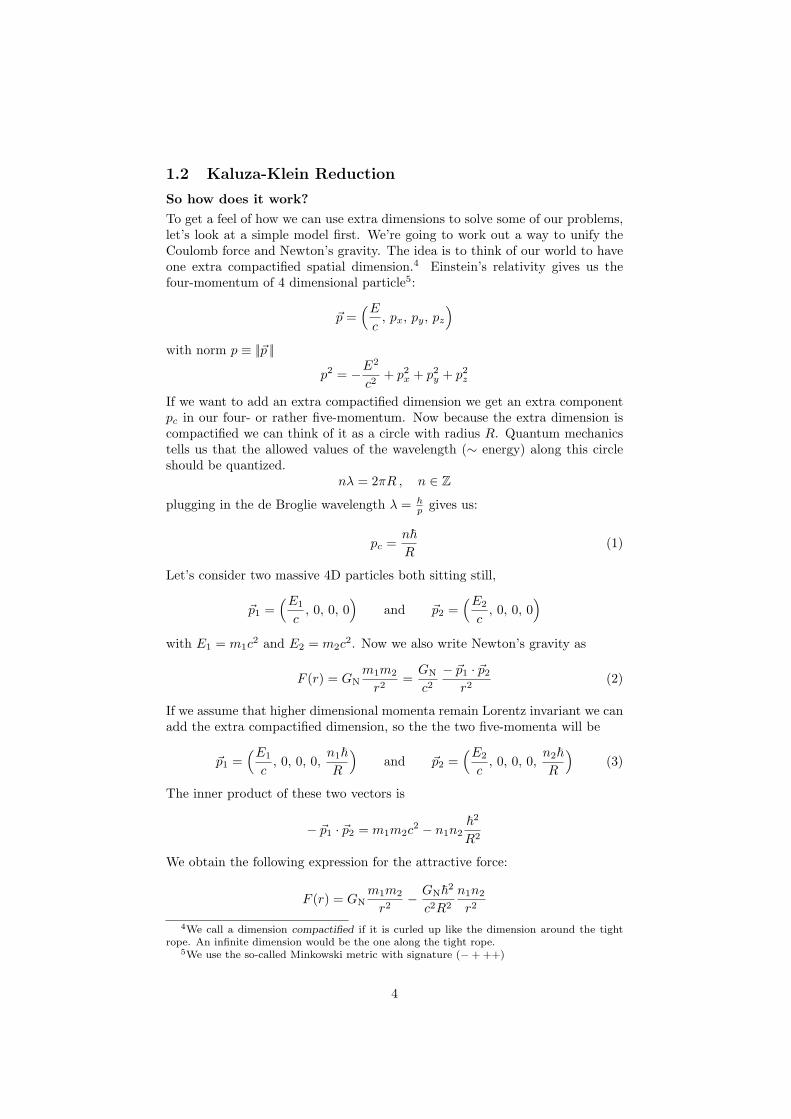
So how does it work?To get a feel of how we can use extra dimensions to solve some of our problems,let’s look at a simple model first. We’re going to work out a way to unify theCoulomb force and Newton’s gravity. The idea is to think of our world to haveone extra compactified spatial dimension.4 Einstein’s relativity gives us thefour-momentum of 4 dimensional particle5:

~p =(E

c, px, py, pz

)with norm p ≡ ||~p ||

p2 = −E2

c2+ p2

x + p2y + p2

z

If we want to add an extra compactified dimension we get an extra componentpc in our four- or rather five-momentum. Now because the extra dimension iscompactified we can think of it as a circle with radius R. Quantum mechanicstells us that the allowed values of the wavelength (∼ energy) along this circleshould be quantized.

nλ = 2πR , n ∈ Z

plugging in the de Broglie wavelength λ = hp gives us:

pc =n~R

(1)

Let’s consider two massive 4D particles both sitting still,

~p1 =(E1

c, 0, 0, 0

)and ~p2 =

(E2

c, 0, 0, 0

)with E1 = m1c

2 and E2 = m2c2. Now we also write Newton’s gravity as

F (r) = GNm1m2

r2=

GN

c2

− ~p1 · ~p2

r2(2)

If we assume that higher dimensional momenta remain Lorentz invariant we canadd the extra compactified dimension, so the the two five-momenta will be

~p1 =(E1

c, 0, 0, 0,

n1~R

)and ~p2 =

(E2

c, 0, 0, 0,

n2~R

)(3)

The inner product of these two vectors is

− ~p1 · ~p2 = m1m2c2 − n1n2

~2

R2

We obtain the following expression for the attractive force:

F (r) = GNm1m2

r2− GN~2

c2R2

n1n2

r2

4We call a dimension compactified if it is curled up like the dimension around the tightrope. An infinite dimension would be the one along the tight rope.

5We use the so-called Minkowski metric with signature (−+ ++)

4

The second term suspiciously resembles Coulomb’s law. If we want to makethis expression match Coulomb’s law we need to set the radius of the extradimension at R = ~

√4πε0GN

ce ≈ 2 · 10−34 m, which is very very small.6 Theformula for the attractive force now reads

F (r) = GNm1m2

r2− 1

4πε0

q1q2

r2= Fg + Fe (4)

with q1 = n1e and q2 = n2e. So there it is, we found a way to get two forcesinto one ”model” via Kaluza-Klein reduction. If you think there’s somethingfishy about the previous calculation I can only say you’re right. We used somequasi-relativistic ways to keep things simple, but nonetheless it gives a goodqualitative notion of how powerful extra dimensions can be. In the next sectionwe will be doing some calculations using large extra dimensions, which mightbe easier to ”see” or detect.

1.3 The Hierarchy Problem

What’s the problem?

To get a glance at how weak gravity is let us take a look at the following example.If you hold a magnet close enough to an iron marble the magnet has no hardtime at all pulling it up. This indicates how much stronger electromagnetismis: the tiny magnet beats a colossal object —the earth— in attracting themarble. If we wish to unify gravity with the other forces there should not besuch a big discrepancy between the scales of the regions on which gravity andelectromagnetism work, but there is. As we just saw, this discrepancy is notjust huge, it’s astronomical. There are more (qualitative) problems, but thisesthetic problem is the one we are dealing with now.

1.3.1 Higher Dimensional Gravity

How would gravity behave in a higher dimensional space?

A way of explaining why gravity is so weak is to say that it propagates in morethan only three spatial dimensions. These extra dimensions should be so smallthat we cannot ”see” them. But before we start talking about gravity in thesesmall compactified dimensions, we need to know how it behaves in general inhigher dimensional spaces.Let’s see what we already know about gravity. We know that in 4D (3 spatial+ 1 time) Newton’s law reads:

F (r) = GNm1m2

r2(5)

The gravitational field ~Φ of just one mass m1 is given by:

~Φ = GNm1

r2r (6)

6In this case R is just about the same size as the Planck length.

5

We can also invoke Gauss’ theorem:∮~Φ · d~s = constant ·mencl.

= 4πGN m1

=∫

sphere

Φr ds

= Φr

∫ 2π

0

dφ

∫ π

0

dθ r2sin θ

= Φr 4πr2

= ΦrS3(r)

where S3(r) is the surface area of a sphere with radius r in our 4 dimensionalworld —the 3 in S3(r) stands for the number of spatial dimensions. With thisresult we can obtain a more general expression for Newton’s gravity in 4D:

F4(r) = Φrm2 = 4πGNm1m2

S3(r)(7)

We see that in 4D the surface area is proportional to the radius as S3(r) ∝ r2.In d spatial dimensions this relation becomes Sd(r) ∝ rd−1. What we want todo now is find the proportionality constant Ωd in

Sd(r) = Ωdrd−1 (8)

so we can work out the gravitational force for d spatial dimensions:

Fd+1(r) = 4πGNm1m2

Sd(r)

To get Ωn we can use the following trick. We can integrate some function intwo ways, in cartesian coordinates and in polar coordinates. In both cases theanswer should be the same. The function we use is a Gaussian e−r2

. Ωn is thepart of the polar integral which is independent of r. We will first work out theCartesian integral.∫

all space

ddr e−r2=

∫ ∞

−∞dr1 e−r2

1 ...

∫ ∞

−∞drd e−r2

d

= (√

π )d

Now let’s see what the polar integral has to offer us.∫all space

ddr e−r2=

∫ ∞

0

dr e−r2∫ 2π

0

dφ

∫ π

0

dθ ... · Jacobian

6

but the Jacobian is proportional to rd−1 so the integral is

=∫ ∞

0

dr rd−1e−r2∫ 2π

0

dφ

∫ π

0

dθ ...

=∫ ∞

0

dr rd−1e−r2Ωd

=Ωd

2

∫ ∞

0

dx xd2−1e−x (subst. x ≡ r2)

=Ωd

2Γ(d

2 )

Here Γ(d2 ) is the Euler-gamma function. We obtain the following expression for

the proportionality constant:

Ωd =2(√

π )d

Γ(d2 )

(9)

A more esthetic way of writing the d + 1 dimensional gravitational force is

Fd+1(r) = Gd+1m1m2

rd−1(10)

with

Gd+1 ≡4πGN

Ωd=

2 Γ(d2 )

(√

π)d−2GN (11)

Let’s check if this is correct for d = 3:

G3+1 =2 Γ( 3

2 )(√

π)3−2GN =

2√

π2√π

GN = GN XSo that’s it, we know how gravity behaves in a higher dimensional space. How-ever, we know that gravity is proportional to 1

r2 so how can this result be right?This result can only be right if the extra dimensions are small enough. So it’stime to start using compactified extra dimensions.

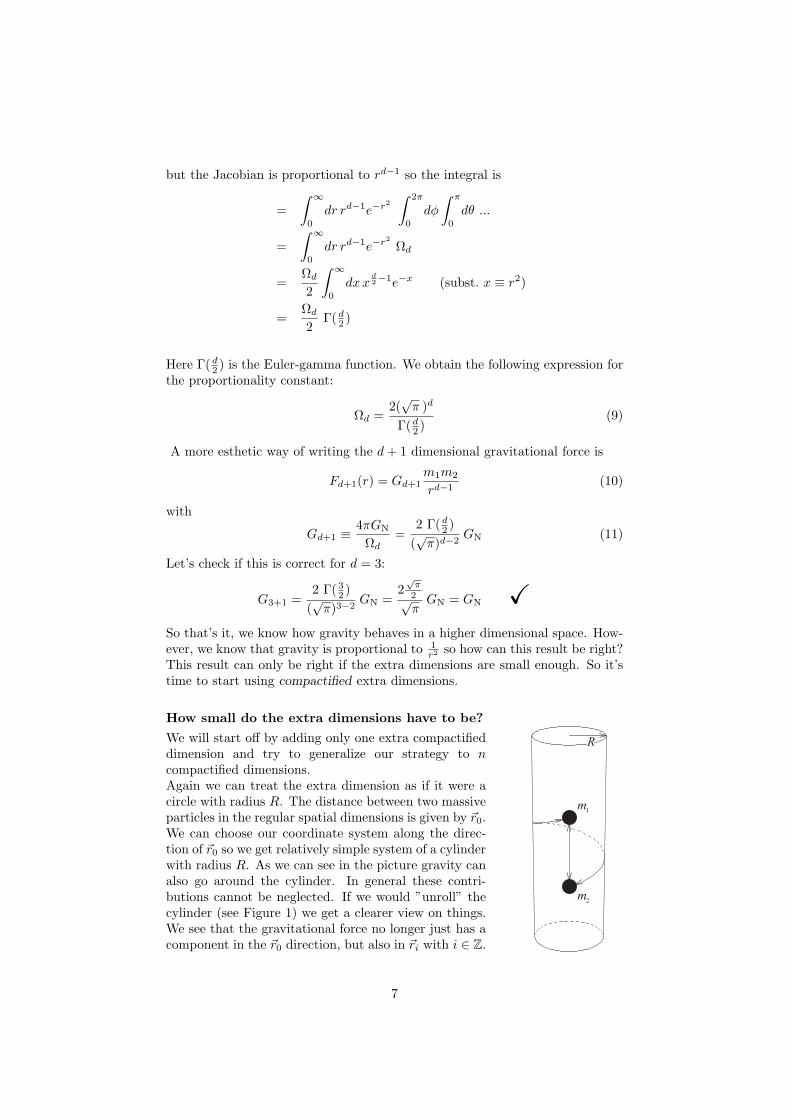
How small do the extra dimensions have to be?

We will start off by adding only one extra compactifieddimension and try to generalize our strategy to ncompactified dimensions.Again we can treat the extra dimension as if it were acircle with radius R. The distance between two massiveparticles in the regular spatial dimensions is given by ~r0.We can choose our coordinate system along the direc-tion of ~r0 so we get relatively simple system of a cylinderwith radius R. As we can see in the picture gravity canalso go around the cylinder. In general these contri-butions cannot be neglected. If we would ”unroll” thecylinder (see Figure 1) we get a clearer view on things.We see that the gravitational force no longer just has acomponent in the ~r0 direction, but also in ~ri with i ∈ Z.

m1

m2

R

7

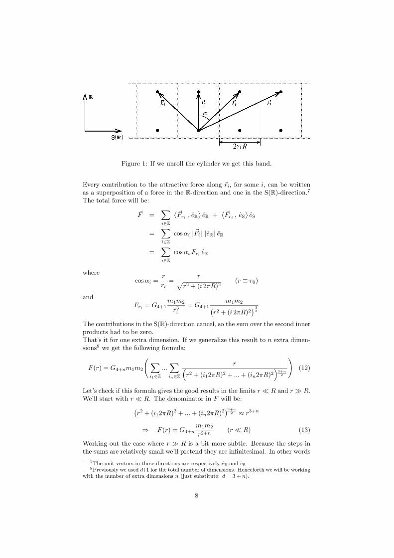
Figure 1: If we unroll the cylinder we get this band.

Every contribution to the attractive force along ~ri, for some i, can be writtenas a superposition of a force in the R-direction and one in the S(R)-direction.7

The total force will be:

~F =∑i∈Z

⟨~Fri

, eR⟩eR +

⟨~Fri , eS

⟩eS

=∑i∈Z

cos αi ||~Fi|| ||eR|| eR

=∑i∈Z

cos αi Fri eR

wherecos αi =

r

ri=

r√r2 + (i 2πR)2

(r ≡ r0)

andFri = G4+1

m1m2

r3i

= G4+1m1m2(

r2 + (i 2πR)2) 3

2

The contributions in the S(R)-direction cancel, so the sum over the second innerproducts had to be zero.That’s it for one extra dimension. If we generalize this result to n extra dimen-sions8 we get the following formula:

F (r) = G4+nm1m2

(∑i1∈Z

...∑in∈Z

r(r2 + (i12πR)2 + ... + (in2πR)2

)3+n

2

)(12)

Let’s check if this formula gives the good results in the limits r R and r R.We’ll start with r R. The denominator in F will be:(

r2 + (i12πR)2 + ... + (in2πR)2)3+n

2 ≈ r3+n

⇒ F (r) = G4+nm1m2

r2+n(r R) (13)

Working out the case where r R is a bit more subtle. Because the steps inthe sums are relatively small we’ll pretend they are infinitesimal. In other words

7The unit-vectors in these directions are respectively eR and eS8Previously we used d+1 for the total number of dimensions. Henceforth we will be working

with the number of extra dimensions n (just substitute: d = 3 + n).

8

we convert the sums into integrals:

F (r) = m1m2G4+n

∫ ∞

−∞di1 ...

∫ ∞

−∞din

r(r2 + (i12πR)2 + ... + (in2πR)2

)3+n

2

How do we get our Newtonian gravity out of this? We will just have to evaluatethis integral. Let’s start with a nice substitution: xm ≡ 2πR

r im with m = 1, ... , nand so the Jacobian is

(r

2πR

)n:

= m1m2G4+n

∫ ∞

−∞di1 ...

∫ ∞

−∞din

r

r3+n(1 + x2

1 + ... + x2n

)3+n

2

( r

2πR

)n

=m1m2

r2

G4+n

Rn· some integral only dependent on n

This looks almost like Newton’s gravity. If we call the n-dependent integral In

and evaluate it we get

In =1

2n+1 (√

π)n−1 Γ( 3+n2 )

and so the gravitational force will be

F (r) =m1m2

r2

G4+nIn

Rn(r R) (14)

If this is correct it means that Newton’s constant must be

GN =G4+nIn

Rn

⇒ Rn =(

G4+nIn

GN

)1/n

(15)

Thus, in the two limits Equation 12 gives the correct results. That’s nice, butthe interesting part is the case in which r ≈ R. We would want to use Equa-tion 14, however we made an approximation which is only valid if r R. Towork around this problem we need to apply a correction which follows fromthe Euler-Maclaurin Integration Formulas.9 We worked out the case of one ex-tra dimension, n = 1 (see Figure 2). We can see that as r approaches R thehigher-dimensional gravity grows stronger than the classical one quite rapidly.

It’s nice to see that gravity grows stronger at short distances, but we cannot yetsee it grows astronomically stronger as required in order to solve the hierarchyproblem. Maybe one extra dimension (with a small radius) is not enough. Inthe next section we will compute the size and number of the extra dimensionsrequired for solving the hierarchy problem.

9We will not to work this out explicitly, because it involves a very long calculation with alot of derivatives and stuff. In stead we’ll just look at the results in Figure 2.

9

Figure 2: The difference between Newton’s gravity and Equation 12.

1.3.2 The ADD Model

What are the Planck and electroweak scales?

A more precise way of saying gravity is weaker than the other forces is to saythat their scales differ. The fundamental scale for the forces in the StandardModel is the scale of electroweak (EW) symmetry breaking:10

MEW ∼ 1 TeV

Gravity’s fundamental scale is the so-called Planck mass (or Planck scale):

MPl =1√GN

∼ 1016 TeV

Gravity needs about 1016 more ”stuff” to work than electromagnetism does.

What does the ADD model stand for?

The following scenario to explain (or alter) the hierarchy problem was firstproposed by Nima Arkani-Hamed, Savas Dimopoulos and Georgi Dvali, ADD forshort. In this model the assumption is that the EW scale is the only fundamentalscale at (very) short distances. If we would invoke compactified extra dimensionswe see that the Planck mass depends on the number n and size R of these extradimensions. The idea is to set

M4+n ∼ MEW ∼ 1 TeV

where M4+n is the Planck mass at n extra dimensions. But what is M4+n? Weshall have to do some dimensional (unit) analysis to calculate this. Let’s startwith the simple case of the regular Planck mass MPl in 4D. The units of ourfundamental constants are:

10Here we use natural units, which means we set c=~=1.

10

[c] = m s−1

[~] = m2kg s−1

[GN] = m3kg−1s−2

The unit of the the Planck mass should be kilograms. Using only c, ~ and GN

we get:

[MPl] =

[√c ~GN

]= kg

Thus we set

MPl =√

c ~GN

≈ 10−8 kg ∼ 1016 TeV (16)

Now let’s calculate M4+n. The unit of Newton’s constant in 4+n dimensions is[G4+n] = m3+nkg−1s−2. To get M4+n we must solve the following equation:

[ci ~j G4+nk] = kg

⇔ (m s−1)i (m2kg s−1)j (m3+nkg−1s−2)k = kg

By using some algebra we get i, j and k as functions of n which yield:

M4+n =(

c1−n ~1+n

G4+n

) 12+n

(17)

but Equation 15 already told us that

Rn =(

G4+nIn

GN

)1/n

If we combine this equation with Equations 16 and 17 (and again apply somealgebra) we get an expression for the radius Rn of the compactified dimensions:11

Rn =

(M2

Pl

M4+nn+2

( c

~

)n 12n+1 (

√π)n−1 Γ

(3+n

2

))1/n

(18)

or in orders of magnitude (and in natural units):

Rn ∼(

M2Pl

M4+nn+2

)1/n

TeV−1 (19)

This is great! Now we know how large the extra dimension have to be, given thenumber of extra dimensions n and the higher dimensional Planck scale M4+n.

So how large do these extra dimension have to be?

Now we can actually set M4+n ∼ MEW ∼ 1 TeV so the compactification radiusRn will be of order:

Rn ∼ 1032n TeV−1 or in SI units : Rn ∼ 10

32n −19 m (20)

11We assume that all the extra dimensions have the same size and are compactified on atorus.

11

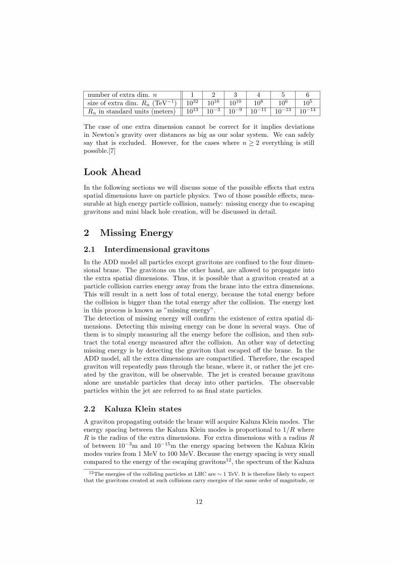
number of extra dim. n 1 2 3 4 5 6size of extra dim. Rn (TeV−1) 1032 1016 1010 108 106 105

Rn in standard units (meters) 1013 10−3 10−9 10−11 10−13 10−14

The case of one extra dimension cannot be correct for it implies deviationsin Newton’s gravity over distances as big as our solar system. We can safelysay that is excluded. However, for the cases where n ≥ 2 everything is stillpossible.[7]

Look Ahead

In the following sections we will discuss some of the possible effects that extraspatial dimensions have on particle physics. Two of those possible effects, mea-surable at high energy particle collision, namely: missing energy due to escapinggravitons and mini black hole creation, will be discussed in detail.

2 Missing Energy

2.1 Interdimensional gravitons

In the ADD model all particles except gravitons are confined to the four dimen-sional brane. The gravitons on the other hand, are allowed to propagate intothe extra spatial dimensions. Thus, it is possible that a graviton created at aparticle collision carries energy away from the brane into the extra dimensions.This will result in a nett loss of total energy, because the total energy beforethe collision is bigger than the total energy after the collision. The energy lostin this process is known as ”missing energy”.The detection of missing energy will confirm the existence of extra spatial di-mensions. Detecting this missing energy can be done in several ways. One ofthem is to simply measuring all the energy before the collision, and then sub-tract the total energy measured after the collision. An other way of detectingmissing energy is by detecting the graviton that escaped off the brane. In theADD model, all the extra dimensions are compactified. Therefore, the escapedgraviton will repeatedly pass through the brane, where it, or rather the jet cre-ated by the graviton, will be observable. The jet is created because gravitonsalone are unstable particles that decay into other particles. The observableparticles within the jet are referred to as final state particles.

2.2 Kaluza Klein states

A graviton propagating outside the brane will acquire Kaluza Klein modes. Theenergy spacing between the Kaluza Klein modes is proportional to 1/R whereR is the radius of the extra dimensions. For extra dimensions with a radius Rof between 10−3m and 10−15m the energy spacing between the Kaluza Kleinmodes varies from 1 MeV to 100 MeV. Because the energy spacing is very smallcompared to the energy of the escaping gravitons12, the spectrum of the Kaluza

12The energies of the colliding particles at LHC are ∼ 1 TeV. It is therefore likely to expectthat the gravitons created at such collisions carry energies of the same order of magnitude, or

12

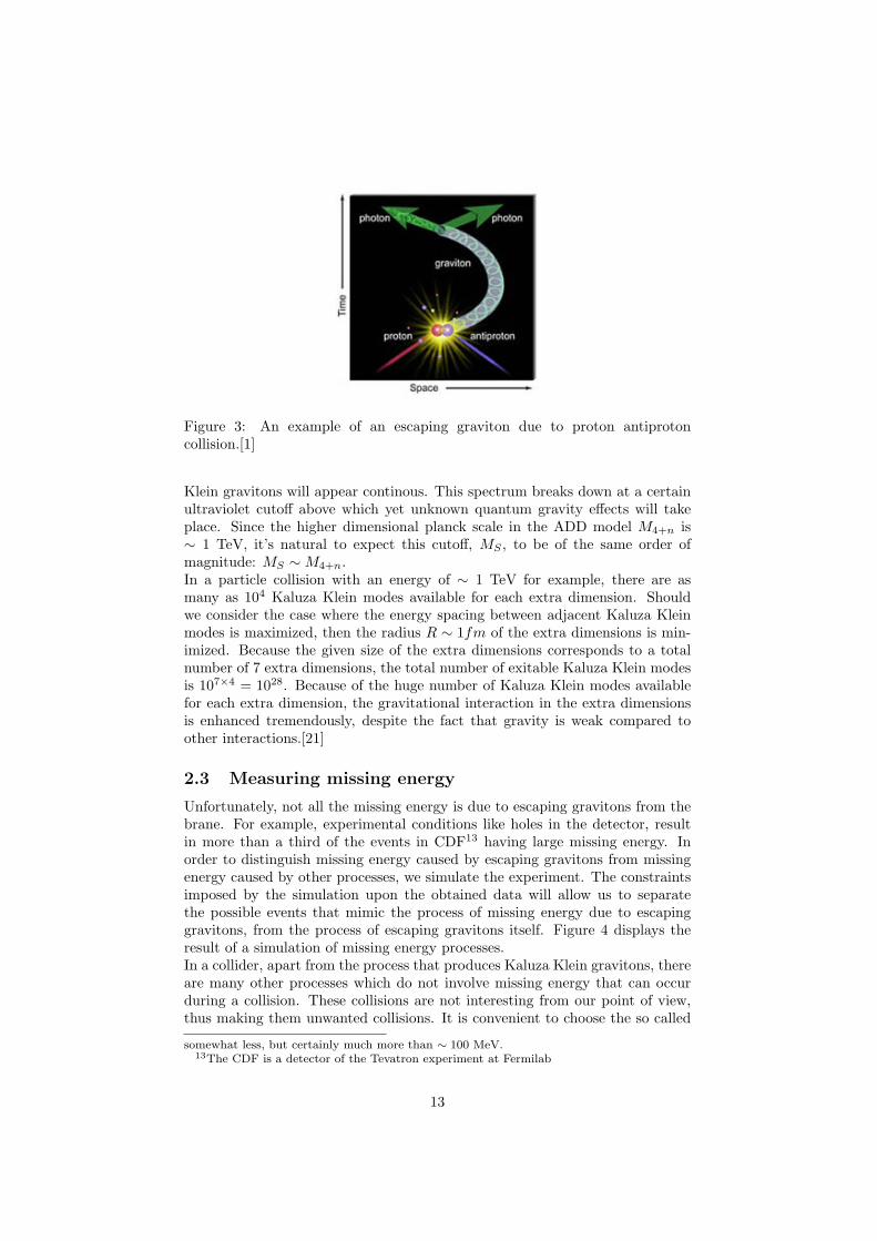
Figure 3: An example of an escaping graviton due to proton antiprotoncollision.[1]

Klein gravitons will appear continous. This spectrum breaks down at a certainultraviolet cutoff above which yet unknown quantum gravity effects will takeplace. Since the higher dimensional planck scale in the ADD model M4+n is∼ 1 TeV, it’s natural to expect this cutoff, MS , to be of the same order ofmagnitude: MS ∼ M4+n.In a particle collision with an energy of ∼ 1 TeV for example, there are asmany as 104 Kaluza Klein modes available for each extra dimension. Shouldwe consider the case where the energy spacing between adjacent Kaluza Kleinmodes is maximized, then the radius R ∼ 1fm of the extra dimensions is min-imized. Because the given size of the extra dimensions corresponds to a totalnumber of 7 extra dimensions, the total number of exitable Kaluza Klein modesis 107×4 = 1028. Because of the huge number of Kaluza Klein modes availablefor each extra dimension, the gravitational interaction in the extra dimensionsis enhanced tremendously, despite the fact that gravity is weak compared toother interactions.[21]

2.3 Measuring missing energy

Unfortunately, not all the missing energy is due to escaping gravitons from thebrane. For example, experimental conditions like holes in the detector, resultin more than a third of the events in CDF13 having large missing energy. Inorder to distinguish missing energy caused by escaping gravitons from missingenergy caused by other processes, we simulate the experiment. The constraintsimposed by the simulation upon the obtained data will allow us to separatethe possible events that mimic the process of missing energy due to escapinggravitons, from the process of escaping gravitons itself. Figure 4 displays theresult of a simulation of missing energy processes.In a collider, apart from the process that produces Kaluza Klein gravitons, thereare many other processes which do not involve missing energy that can occurduring a collision. These collisions are not interesting from our point of view,thus making them unwanted collisions. It is convenient to choose the so called

somewhat less, but certainly much more than ∼ 100 MeV.13The CDF is a detector of the Tevatron experiment at Fermilab

13

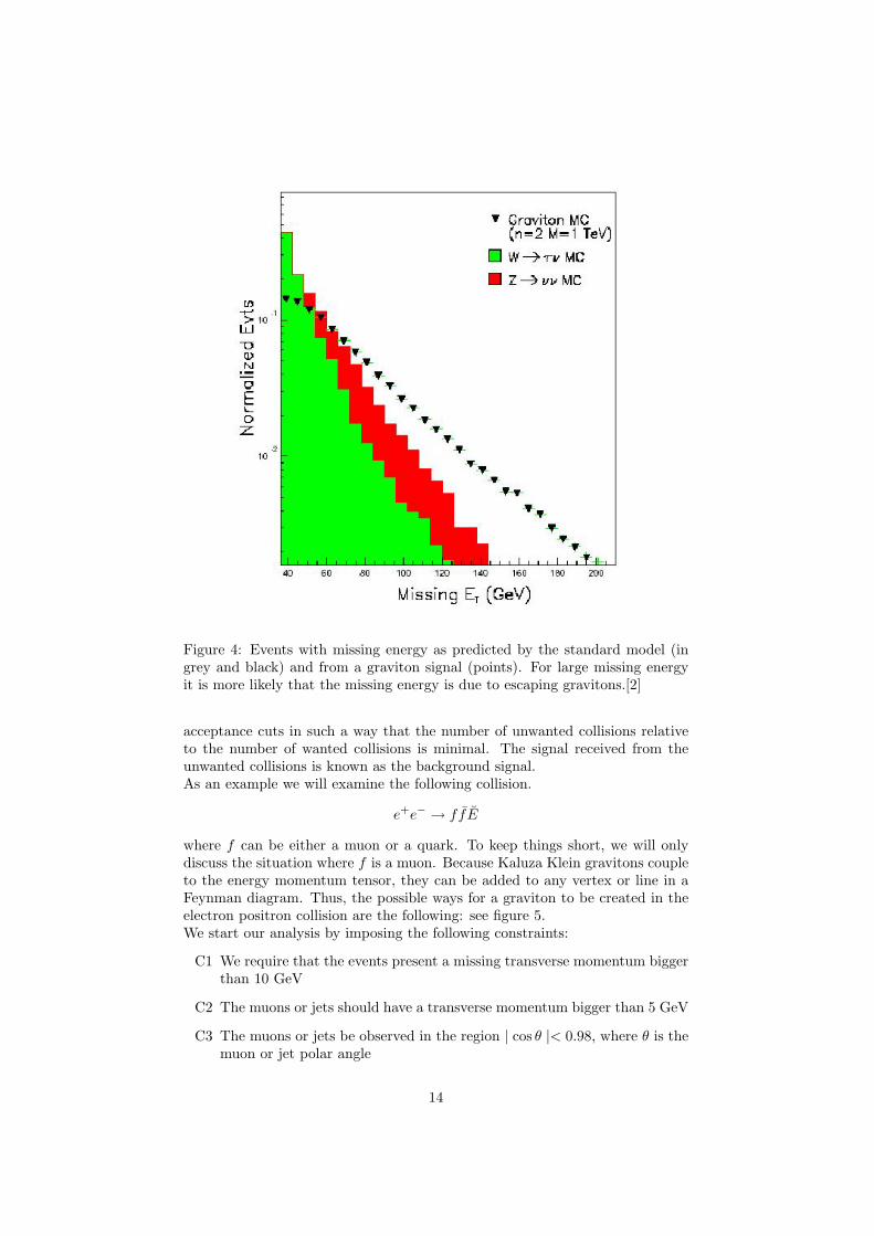
Figure 4: Events with missing energy as predicted by the standard model (ingrey and black) and from a graviton signal (points). For large missing energyit is more likely that the missing energy is due to escaping gravitons.[2]

acceptance cuts in such a way that the number of unwanted collisions relativeto the number of wanted collisions is minimal. The signal received from theunwanted collisions is known as the background signal.As an example we will examine the following collision.

e+e− → ffE

where f can be either a muon or a quark. To keep things short, we will onlydiscuss the situation where f is a muon. Because Kaluza Klein gravitons coupleto the energy momentum tensor, they can be added to any vertex or line in aFeynman diagram. Thus, the possible ways for a graviton to be created in theelectron positron collision are the following: see figure 5.We start our analysis by imposing the following constraints:

C1 We require that the events present a missing transverse momentum biggerthan 10 GeV

C2 The muons or jets should have a transverse momentum bigger than 5 GeV

C3 The muons or jets be observed in the region | cos θ |< 0.98, where θ is themuon or jet polar angle

14

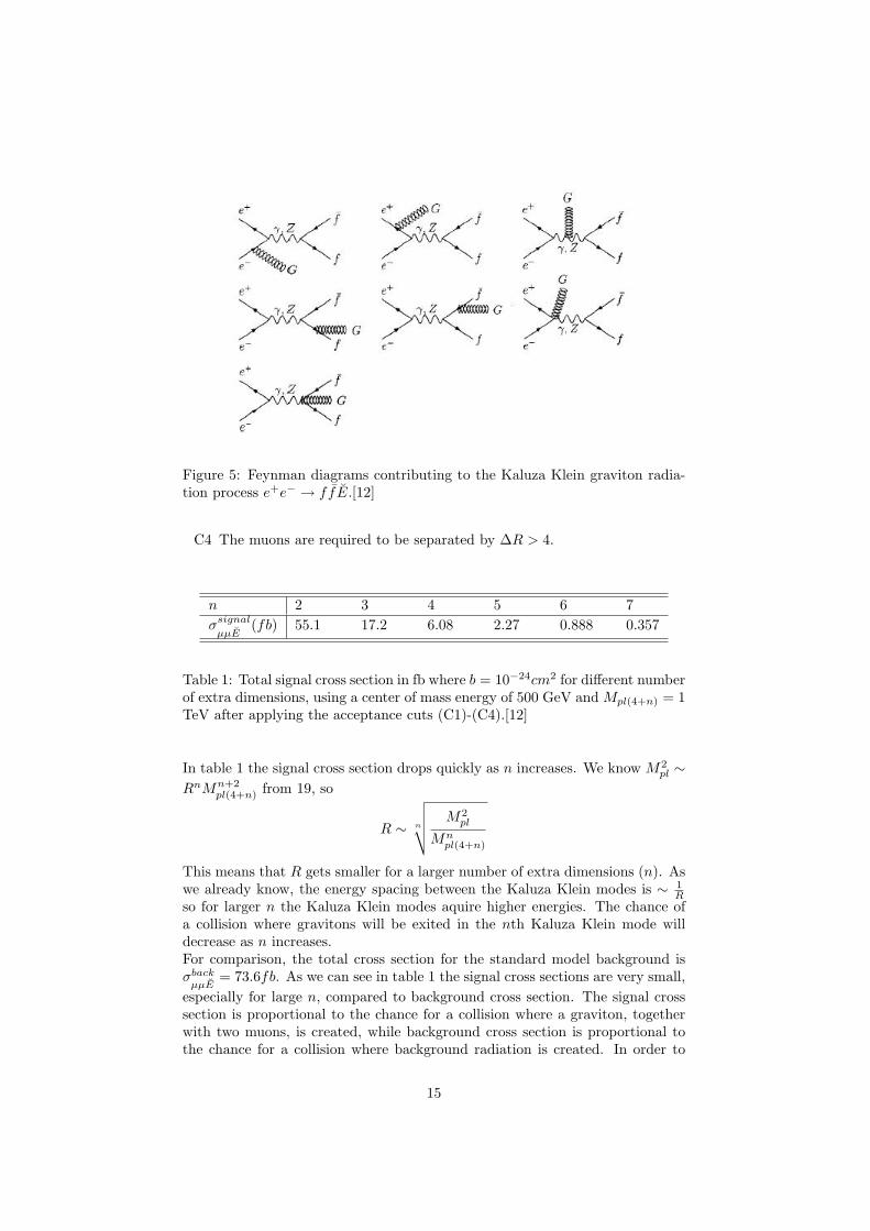
Figure 5: Feynman diagrams contributing to the Kaluza Klein graviton radia-tion process e+e− → ffE.[12]

C4 The muons are required to be separated by ∆R > 4.

n 2 3 4 5 6 7σsignal

µµE(fb) 55.1 17.2 6.08 2.27 0.888 0.357

Table 1: Total signal cross section in fb where b = 10−24cm2 for different numberof extra dimensions, using a center of mass energy of 500 GeV and Mpl(4+n) = 1TeV after applying the acceptance cuts (C1)-(C4).[12]

In table 1 the signal cross section drops quickly as n increases. We know M2pl ∼

RnMn+2pl(4+n) from 19, so

R ∼ n

√√√√ M2pl

Mnpl(4+n)

This means that R gets smaller for a larger number of extra dimensions (n). Aswe already know, the energy spacing between the Kaluza Klein modes is ∼ 1

Rso for larger n the Kaluza Klein modes aquire higher energies. The chance ofa collision where gravitons will be exited in the nth Kaluza Klein mode willdecrease as n increases.For comparison, the total cross section for the standard model background isσback

µµE= 73.6fb. As we can see in table 1 the signal cross sections are very small,

especially for large n, compared to background cross section. The signal crosssection is proportional to the chance for a collision where a graviton, togetherwith two muons, is created, while background cross section is proportional tothe chance for a collision where background radiation is created. In order to

15

investigate the Kaluza Klein gravitons, it is therefore necessary to maximize thesignal cross section relative to the background cross section.

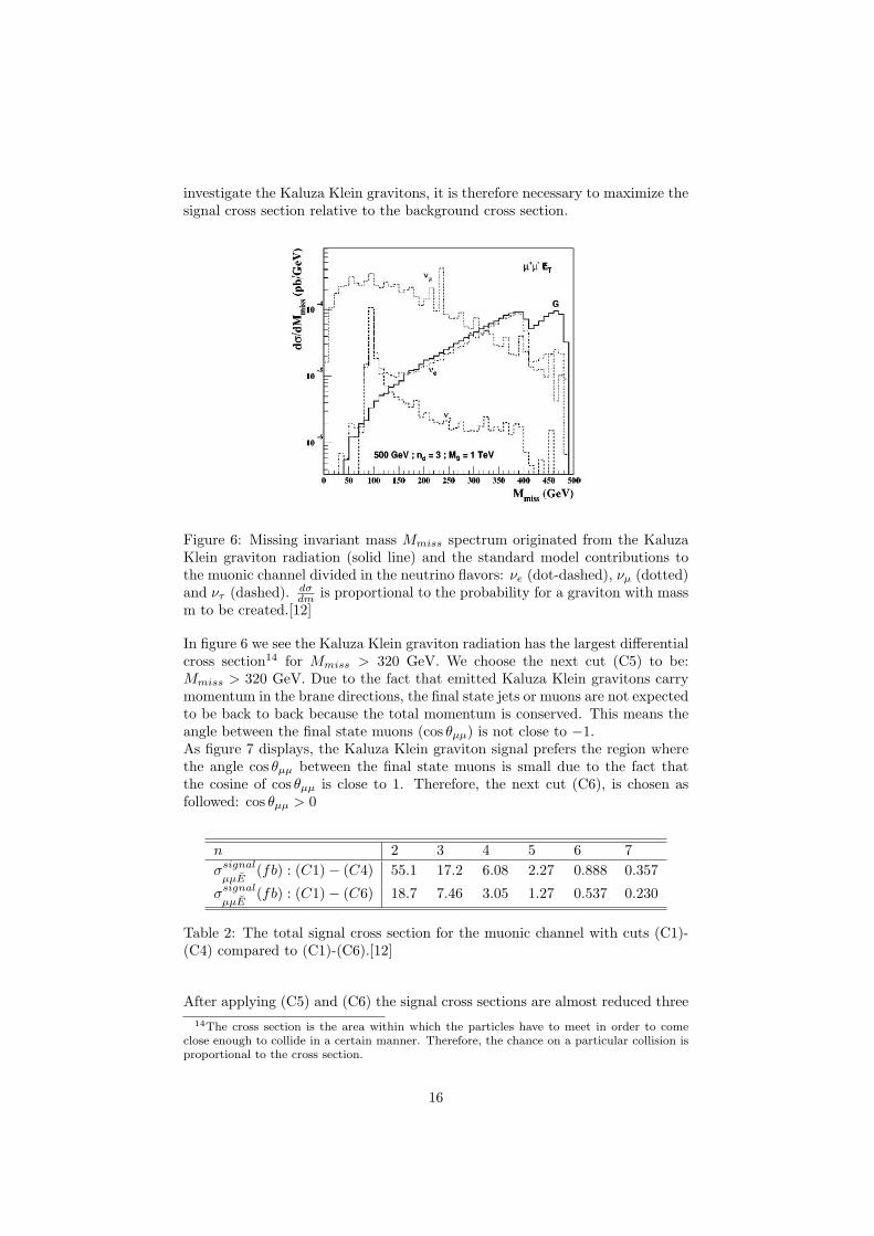
Figure 6: Missing invariant mass Mmiss spectrum originated from the KaluzaKlein graviton radiation (solid line) and the standard model contributions tothe muonic channel divided in the neutrino flavors: νe (dot-dashed), νµ (dotted)and ντ (dashed). dσ

dm is proportional to the probability for a graviton with massm to be created.[12]

In figure 6 we see the Kaluza Klein graviton radiation has the largest differentialcross section14 for Mmiss > 320 GeV. We choose the next cut (C5) to be:Mmiss > 320 GeV. Due to the fact that emitted Kaluza Klein gravitons carrymomentum in the brane directions, the final state jets or muons are not expectedto be back to back because the total momentum is conserved. This means theangle between the final state muons (cos θµµ) is not close to −1.As figure 7 displays, the Kaluza Klein graviton signal prefers the region wherethe angle cos θµµ between the final state muons is small due to the fact thatthe cosine of cos θµµ is close to 1. Therefore, the next cut (C6), is chosen asfollowed: cos θµµ > 0

n 2 3 4 5 6 7σsignal

µµE(fb) : (C1)− (C4) 55.1 17.2 6.08 2.27 0.888 0.357

σsignal

µµE(fb) : (C1)− (C6) 18.7 7.46 3.05 1.27 0.537 0.230

Table 2: The total signal cross section for the muonic channel with cuts (C1)-(C4) compared to (C1)-(C6).[12]

After applying (C5) and (C6) the signal cross sections are almost reduced three14The cross section is the area within which the particles have to meet in order to come

close enough to collide in a certain manner. Therefore, the chance on a particular collision isproportional to the cross section.

16

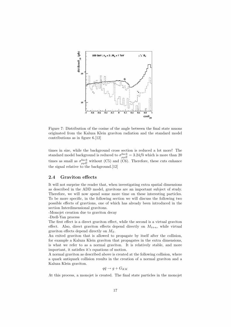
Figure 7: Distribution of the cosine of the angle between the final state muonsoriginated from the Kaluza Klein graviton radiation and the standard modelcontributions as in figure 6.[12]

times in size, while the background cross section is reduced a lot more! Thestandard model background is reduced to σback

µµE= 3.24fb which is more than 20

times as small as σbackµµE

without (C5) and (C6). Therefore, these cuts enhancethe signal relative to the background.[12]

2.4 Graviton effects

It will not surprise the reader that, when investigating extra spatial dimensionsas described in the ADD model, gravitons are an important subject of study.Therefore, we will now spend some more time on these interesting particles.To be more specific, in the following section we will discuss the following twopossible effects of gravtions, one of which has already been introduced in thesection Interdimensional gravitons.-Monojet creation due to graviton decay-Drell-Yan processThe first effect is a direct graviton effect, while the second is a virtual gravitoneffect. Also, direct graviton effects depend directly on M4+n, while virtualgraviton effects depend directly on MS .An exited graviton that is allowed to propagate by itself after the collision,for example a Kaluza Klein graviton that propagates in the extra dimensions,is what we refer to as a normal graviton. It is relatively stable, and moreimportant, it satisfies it’s equations of motion.A normal graviton as described above is created at the following collision, wherea quark antiquark collision results in the creation of a normal graviton and aKaluza Klein graviton.

qq → g + GKK

At this process, a monojet is created. The final state particles in the monojet

17

can be detected by a non conservation in transverse momentum. Also, themonojet will lead to an amplification of the tail of transverse energy spectrum.Apart from collisions where normal gravitons are excited, it’s also possible for aso called virtual graviton to be created. Virtual, in a sense, means that if we lookat the Feynman diagram that describes the collision, the graviton is not allowedto leave the diagram. For example, all the Feynman diagrams that are shown infigure 5, display normal gravitons that are allowed to leave the diagram. Virtualgravitons on the other hand, are stuck between the two vertices. What is meantby ”not allowed to leave the diagram” is that the gravitons are not able to liveby themselves. This is a direct consequence of the fact that the virtual gravitonsdo not satisfy their equations of motion15. Thus, they are only allowed to existin some sort of intermediate state, which is what the line connecting the twovertices in the Feynman diagram stands for.Virtual graviton effects take place at the Drell-Yan process, mentioned above.Note that this is just one of the many processes where virutal graviton effects cantake place. The Drell-Yan processes in the presence of large extra dimensionsis shown in figure 8.

Figure 8: Feynman diagrams for the modified Drell-Yan production in the pres-ence of large extra dimensions.[21]

Both processes noted above have already been studied at Tevatron Fermilabwith the CFD and DØ detectors. We will discuss the results obtained at Teva-tron Fermilab ref shortly. Results from the monojet searches in Run 1 aresummarized in the next table.

Experiment and channel n = 2 n = 3 n = 4 n = 5 n = 6 n = 7DØ monojets, K = 1 0.89 0.73 0.86 0.64 0.63 0.62DØ monojets, K = 1.3 1.99 0.80 0.73 0.66 0.65 0.63CDF monojets, K = 1 1.00 0.77 0.71CDF monojets, K = 1.3 1.06 0.80 0.73

Table 3: Individual 95% CL lower limits on the fundamental Planck scale MD

(in TeV) in the ADD model from the CDF and DØ experiments. Ordering ofthe results is chronological.[21]

It is possible to compute the chance of a certain collision to take place from theaccompanying Feynman diagram. Figure 9 shows both thecalculated events per transverse energy of the monojet, as well as the measuredevents per transverse energy of the monojet.

15Virtual gravitons don’t satisfy E2 = m2c4 + p2c2

18

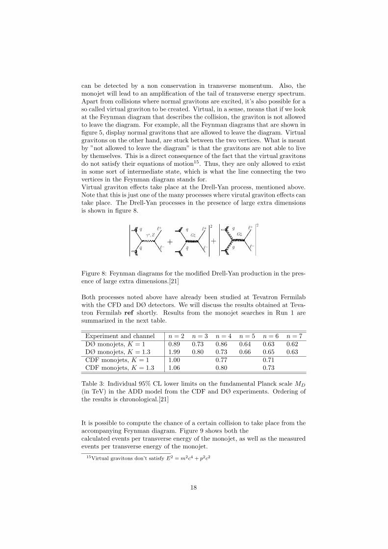
Figure 9: Transverse energy of the leading jet in the DØ monojet analysis.Points are data, while the histogram is the expected background radiation. Theshadow band corresponds to the change in the jet energy scale (JES) of +/- onestandard deviation.[21]

At Tevatron Run 2 the Drell-Yan process was investigated using both the CDFand the DØ detectors. Figure 10 shows the invariant mass spectra of the pro-duced dielectrons16 for two different topologies. As can be seen from figure 10,the Kaluza Klein graviton contribution to the signal is dominant in the regionwhere the signal exceeds the expected background, rather than the interferenceterm which causes virtual graviton exchange.[21]

3 Black holes

A lot of new theories in physics suggest extra dimensions or need extra dimen-sions to be valid. Until now there is no evidence for the existence of extradimensions but the investigation of mini black holes produced in particle col-liders could give insight in the unexplored world of extradimensional physics.If the fundamental planck scale is of order a TeV, as the case in some extra-dimensions scenarios, future colliders such as the Large Hadron Collider (LHC)will be black hole factories. In this section we investigate the behavior of blackholes in more dimensions and the possibility of creating them at the LHC.

3.1 Black holes in general

A black hole is a body which has such a great mass that not even light canescape from it due to the gravitational field surrounding the black hole. Beforewe will deal with black holes in accelerators we will take a look at black holesin general.

16Indeed, in this case the leptons in figure 8 are electrons.

19

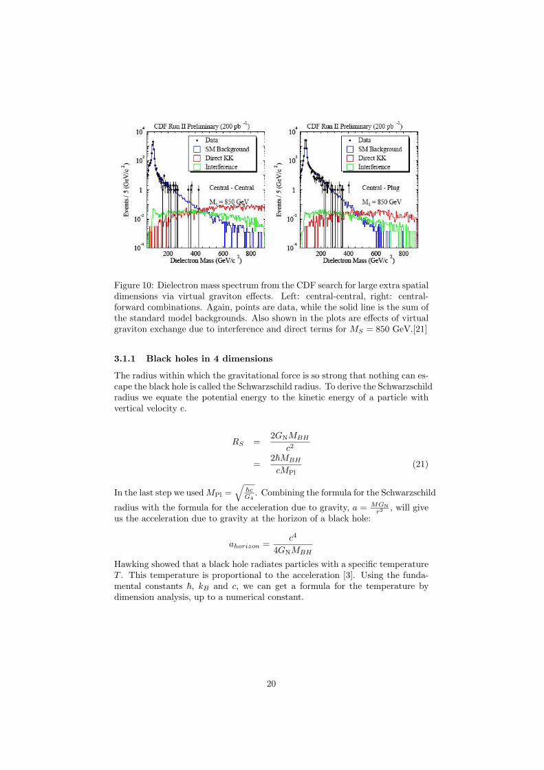
Figure 10: Dielectron mass spectrum from the CDF search for large extra spatialdimensions via virtual graviton effects. Left: central-central, right: central-forward combinations. Again, points are data, while the solid line is the sum ofthe standard model backgrounds. Also shown in the plots are effects of virtualgraviton exchange due to interference and direct terms for MS = 850 GeV.[21]

3.1.1 Black holes in 4 dimensions

The radius within which the gravitational force is so strong that nothing can es-cape the black hole is called the Schwarzschild radius. To derive the Schwarzschildradius we equate the potential energy to the kinetic energy of a particle withvertical velocity c.

RS =2GNMBH

c2

=2~MBH

cMPl(21)

In the last step we used MPl =√

~cG4

. Combining the formula for the Schwarzschild

radius with the formula for the acceleration due to gravity, a = MGNr2 , will give

us the acceleration due to gravity at the horizon of a black hole:

ahorizon =c4

4GNMBH

Hawking showed that a black hole radiates particles with a specific temperatureT . This temperature is proportional to the acceleration [3]. Using the funda-mental constants ~, kB and c, we can get a formula for the temperature bydimension analysis, up to a numerical constant.

20

[T ] = K

[ahorizon] =m

s2

[~] =kgm2

s

[kB ] =kgm2

s2K

[c] =m

s

We need to satisfy the following equation:

[T ] = [ahorizon]α[~]β [kB ]γ [c]δ

This gives a system of equations which can be solved. We get:α = 1 β = 1 γ = −1 δ = −1.Now we can write down an explicit formula for the Hawking Temperature in 4dimensions. The numerical constant is (8π)−1.

T =~c3

8πGNMBHkB(22)

Note that the temperature of the black hole increases as the mass decreases. Ablack hole gets hotter as it decays, which causes the decay-process to accelerate.

We know from thermodynamics that the integrating factor of the entropy is theinverse of the temperature. Using the first law of thermodynamics, dE = TdS,we find [19]

S =∫

c2

T (MBH)dM

=4πGNkBM2

BH

~c(23)

= kBπR2

S

L2Pl

In the last step we used equation 21 and LPl =√

GN~c3 .

If you consider a black hole in a canonical way, the energy density of a blackhole is given by the Stefan-Boltzmann law. To compute the luminosity of ablack hole we have to multiply the energy density by the surface area of theblack hole.

L = 4πRSσT 4

=σ~4c8

162π3G2Nk4

B

∗ 1M2

BH

(24)

Note that the luminosity of a black hole is inversely proportional to the squareof the mass.

21

3.1.2 Black holes in (4+n) dimensions

The black holes that will possibly be formed at the LHC are smaller than theradius of the extra dimensions. The topology of the object can be assumed to bespherical symmetric in 4+n dimensions. We will use a semi-classical way of de-riving the properties of the black hole. Our approach is valid if MBH M4+n.[19] [20]

To derive the schwarzschild radius of a (4+n)-dimensional black hole, we haveto equate the (4+n)-dimensional potential energy needed to take a particle awayfrom the surface of a black hole to infinity, to the kinetic energy of a particlewith vertical velocity c. The (4+n)-dimensional potential energy is given by

U =1

n + 1∗ G4+nMBHm

Rn+1S

(25)

The kinetic energy in (4+n) dimensions is 12mc2 because the particle moves

in a two dimensional plane. Now it is easy to see that the (4+n)-dimensionalschwarzschild radius is given by

RH =(

2G4+nMBH

(n + 1)c2

) 1n+1

=

(2

n + 1MBH

Mn+24+n

) 1n+1 ~

c

In the last step we used M4+n = n+2

√~n+1

cn−1G4+n. Setting ~ and c equal to 1, which

is often done in theoretical physics, gives us a nice formula for the schwarzschildradius in 4+n dimensions.

RH =(

2n + 1

MBH

M4+n

) 1n+1 1

M4+n(26)

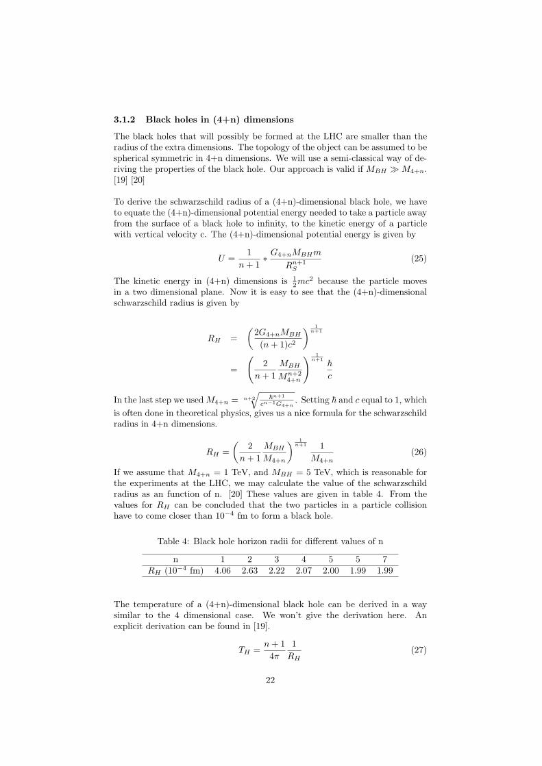
If we assume that M4+n = 1 TeV, and MBH = 5 TeV, which is reasonable forthe experiments at the LHC, we may calculate the value of the schwarzschildradius as an function of n. [20] These values are given in table 4. From thevalues for RH can be concluded that the two particles in a particle collisionhave to come closer than 10−4 fm to form a black hole.

Table 4: Black hole horizon radii for different values of n

n 1 2 3 4 5 5 7RH (10−4 fm) 4.06 2.63 2.22 2.07 2.00 1.99 1.99

The temperature of a (4+n)-dimensional black hole can be derived in a waysimilar to the 4 dimensional case. We won’t give the derivation here. Anexplicit derivation can be found in [19].

TH =n + 14π

1RH

(27)

22

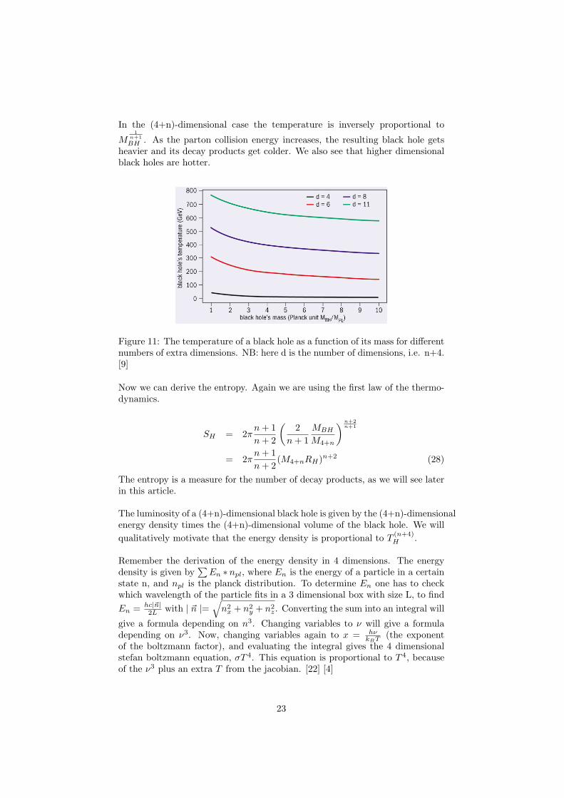
In the (4+n)-dimensional case the temperature is inversely proportional to

M1

n+1BH . As the parton collision energy increases, the resulting black hole gets

heavier and its decay products get colder. We also see that higher dimensionalblack holes are hotter.

Figure 11: The temperature of a black hole as a function of its mass for differentnumbers of extra dimensions. NB: here d is the number of dimensions, i.e. n+4.[9]

Now we can derive the entropy. Again we are using the first law of the thermo-dynamics.

SH = 2πn + 1n + 2

(2

n + 1MBH

M4+n

)n+2n+1

= 2πn + 1n + 2

(M4+nRH)n+2 (28)

The entropy is a measure for the number of decay products, as we will see laterin this article.

The luminosity of a (4+n)-dimensional black hole is given by the (4+n)-dimensionalenergy density times the (4+n)-dimensional volume of the black hole. We willqualitatively motivate that the energy density is proportional to T

(n+4)H .

Remember the derivation of the energy density in 4 dimensions. The energydensity is given by

∑En ∗ npl, where En is the energy of a particle in a certain

state n, and npl is the planck distribution. To determine En one has to checkwhich wavelength of the particle fits in a 3 dimensional box with size L, to findEn = hc|~n|

2L with | ~n |=√

n2x + n2

y + n2z. Converting the sum into an integral will

give a formula depending on n3. Changing variables to ν will give a formuladepending on ν3. Now, changing variables again to x = hν

kBT (the exponentof the boltzmann factor), and evaluating the integral gives the 4 dimensionalstefan boltzmann equation, σT 4. This equation is proportional to T 4, becauseof the ν3 plus an extra T from the jacobian. [22] [4]

23

Now we will give the analogue in 4+n dimensions. To determine En one hasto check which wavelength of the particle fits in a (3+n) dimensional box withsize L. This will give En = hc|~n|

2L , but now | ~n | is the absolute value of a (3+n)

dimensional vector: | ~n |=√

n21 + n2

2 + · · ·n23+n. Converting the sum into an

integral gives a formula depending on n3+n and changing of variables twice willgive a formula depending of T 4+n, where the ’extra T ’ again comes from theJacobian. This time we cannot evaluate the integral exact but we know it willjust give a constant which we will call σ4+n. Note that this constant is not thesame at the 4 dimensional σ. So the (4+n) dimensional energy density is givenby

ε = σ4+nT 4+n

The volume of a sphere in 4+n dimensions is given by

V4+n(R) =2π

n+32

Γ(n+32 )

Rn+2

as has been derived in section 1, equations 8 and 9. The luminosity is propor-tional to

LH ∼ Rn+2H T

(n+4)H

∼ M− 2

n+1BH (29)

3.2 Black hole production

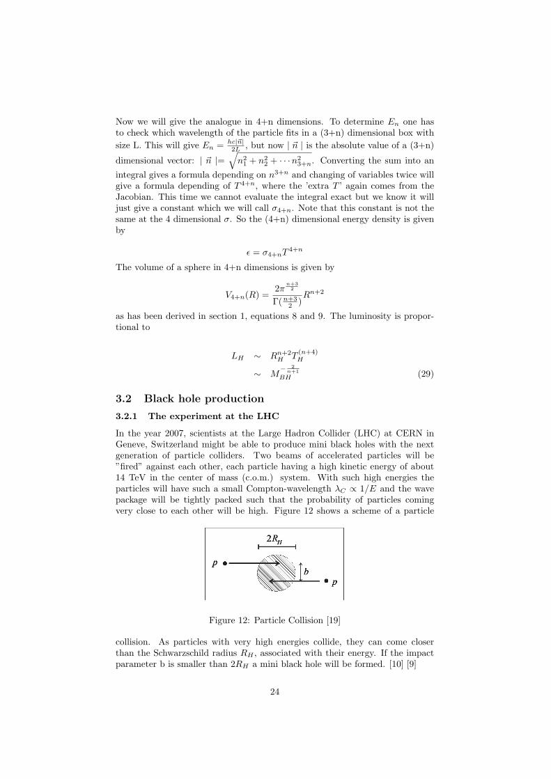
3.2.1 The experiment at the LHC

In the year 2007, scientists at the Large Hadron Collider (LHC) at CERN inGeneve, Switzerland might be able to produce mini black holes with the nextgeneration of particle colliders. Two beams of accelerated particles will be”fired” against each other, each particle having a high kinetic energy of about14 TeV in the center of mass (c.o.m.) system. With such high energies theparticles will have such a small Compton-wavelength λC ∝ 1/E and the wavepackage will be tightly packed such that the probability of particles comingvery close to each other will be high. Figure 12 shows a scheme of a particle

Figure 12: Particle Collision [19]

collision. As particles with very high energies collide, they can come closerthan the Schwarzschild radius RH , associated with their energy. If the impactparameter b is smaller than 2RH a mini black hole will be formed. [10] [9]

24

3.2.2 Energy needed to form a black hole

The Schwarzschild radius RH of a (4 + n) dimensional black hole with mass Mis given by equation 26. We suppose the Planck mass M4+n to be of order 1TeV in (4 + n) dimensions. Thus, a black hole with mass of order M4+n has aSchwarzschild radius

RH ≈ LPl = 1/M4+n (30)

We want the Compton wavelength λC of the particles to be in the same orderof magnitude. Assuming λC ≈ 1/E (and we can do that since by dimensionalanalysis we can show that the fundamental constants must be the same in bothcases RH and λC and no big extra factors occur) we need a c.o.m. energy oforder M4+n to get λC close to RH . Thus the energy needed to form a blackhole will be of order E = 1 TeV. The next generation of particle acceleratorsat the LHC will be able to produce such high energies in the coming years.[10][14] [18]

3.2.3 Cross section

The cross section is the area within which the partons have to meet to comeclose enough to form a black hole. Arguments along the line of Thorne’s hoopconjecture indicate that a black hole forms when partons collide at impact pa-rameter b that is less than the Schwarzschild radius RH corresponding to E [14].This cross section can be approximated by the classical geometric cross section

σ(M) ≈ πR2H (31)

and contains no small coupling constants. This approximation of the crosssection has been and is still under debate, but it seems to be justified at leastup to energies of ≈ 10M4+n [19]. The cross section of a parton collision withc.o.m. energy

√s ≈ M4+n ≈ TeV is of order (1TeV )−2 ≈ 400pb.[19] [14] [23]

3.2.4 Differential cross section

We will need the differential cross section dσdM to be able to compute the number

of black holes that will be formed with a certain mass MBH at a c.o.m. en-ergy

√s. It is given by summation over all possible parton interactions, which

is expressed in the functions fA(x1, s), fB(x2, s) giving the distribution of thepartons within the protons, and integration over the momentum fractions. Wewill give the equation here but refer for further explanation to [19].

dσ

dM=∑

A1,B2

∫ 1

0

dx12√

s

x1sfA(x1, s)fB(x2, s)σ(M,d) (32)

It is complicated to calculate this term. We will give a numerical evaluation ofit, shown in Figure 13, left. By integrating equation 32 we get the total crosssection. The plot in Figure 13, right, shows the total cross section of a black holewith mass Mf = M4+n = 1TeV as a function of the collision energy

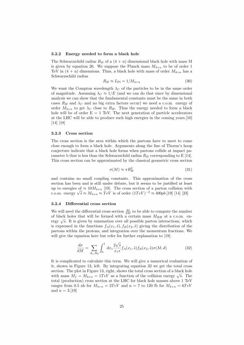
√s. The

total (production) cross section at the LHC for black hole masses above 1 TeVranges from 0.5 nb for M4+n = 2TeV and n = 7 to 120 fb for M4+n = 6TeVand n = 3.[19]

25

Figure 13: Left: Differential cross section for black hole production in proton-proton-collisions at the LHC for M4+n = 1TeV , Right: Integrated total crosssection as a function of the collision energy

√s, both plots deal with the case d

= 6 extra dimensions. [19]

3.2.5 Number of produced black holes per year

According to [11], the LHC will have a (estimated) peak luminosity of 30fb−1/year.This would result in a black hole production rate of 107/year. According to [19]the luminosity is going to be about L = 1033cm−2s−1, which, at a c.o.m. energyof 14 TeV, would give birth to about 109 black holes per year. This is aboutone black hole per second! [19] [11]

3.3 Black hole decay

3.3.1 Balding phase, evaporation phase, Planck phase

Decay of spinning black holes can be divided in three phases.Phase 1: The balding phase in which the black hole loses its ’hair’, that meanslost of multipole moments through the emission of (classical) radiation.Phase 2: The evaporation phase, evaporation through emission of Hawking ra-diation, which starts with a brief spin-down phase, giving away its angularmomentum, followed by the Schwarzschild phase: the emitted particles carrysignatures of mass, entropy and temperature of the black hole.Phase 3: The Planck phase, when the mass of the black hole approaches M4+n

and the black hole’s final decay takes place by emission of a few quanta with cor-responding Planck-scale-energies. There are two possibilities for an end state:Either the black hole decays completely or some stable remnant is left, whichcarries away the remaining energy. Information is lost.[19] [14] [15]

3.3.2 The evaporation phase: Hawking radiation

In the past scientists thought that there was no way for energy to escape a blackhole, they thought of a black hole as a massive object letting nothing escape theso-called Schwarzschild-radius. But then there was Hawking, who published anew theory in 1975. When taking quantum theory in account, black holes canradiate according to Hawking’s theory because of random vacuum fluctuations

26

near the Schwarzschild-radius.Virtual particle pairs are constantly being created near the horizon of a blackhole. Normally, a particle-antiparticle pair annihilates quickly after creation.However, near the horizon of a black hole it’s possible for one particle to fallinto the black hole, while the other particle escapes as Hawking radiation. Inthis case the antiparticle with negative energy falling into the black hole takesenergy of the black hole that escapes by means of the other particle. [19] [5][17] [15]

3.3.3 Black body radiation

Hawking showed that the radiation of a black hole can be seen as radiation ofa black body with a specific temperature T. This implicates the use of thermo-dynamics to calculate various properties of a black hole. The particle spectrumof the radiation of a black hole can be seen as a thermal spectrum (Planck /Maxwell-Boltzman distribution). Since we are dealing with black holes of verysmall mass i.e. only few particles, one could suggest that the distributions arenot valid anymore. But since the black holes that are going to be produced havea mass of order TeV and emitted particles will have an energy of order 10 GeV,the spectra will keep their validity. Furthermore the radiated particles can beseen as massless because their total energy will exceed their mass energy by far.Therefore all kinds of particles of the Standard Model (SM) will be producedwith the same probability. [19] [5]

3.3.4 Evaporation rate and life time of a (mini-)black hole

The luminosity of a black hole is the energy it loses per second through radiation.

L = −dE

dt(33)

The energy of a black hole of mass M has amount E = Mc2, therefore:

L = −c2 dM

dt(34)

Combining with equation 24 we get the evaporation rate:

dM

dt≈ − 1

15π83

c4~G2

NM20

(35)

where M0 is the initial mass of the black hole at the time being investigated.As the black hole loses mass, its temperature (see equation 22) increases and sodoes dM

dt which results in an even quicker decay.Integration over t reveals an estimate τ for the lifetime of a black hole.

τ ≈ 15π83 G2N

c4~M3

0 ≈ 1059

(M0

M

)3

Gyr (36)

For a mini-black hole or a black hole with small mass, say MBH ≈ MPl, dMdt

should be calculated by using the micro canonical ensemble, applying the lawsof statistical mechanics (see [19]) since, using Hawking radiation and the Stefan-Boltzman law for black body radiation, dM

dt goes to infinity as MBH approaches

27

0. dMdt can be calculated using the canonical ensemble, too, see [19]. Then the

variation of the mass is given by

dMBH

dt=

4π3

45M2

BH

M4Pl

exp[−4π(MBH/MPl)2]∫ MBH

0

(MBH−x)3exp[4π(x/MPl)2] dx

(37)For further explanation and derivation of this formula see [19].

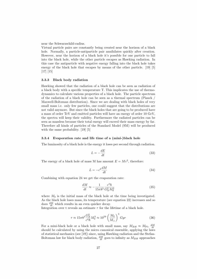
Figure 14: Canonical contra micro canonical. [19]

Figure 14 shows the canonical and micro canonical results. As we can see, thecanonical evaporation rate diverges as M goes to 0 whereas the micro canonicaldrops back after having passed a maximum near MBH = MPl.

In (4 + n) dimensions we get for the evaporation rate (see [19]:

dMBH

dt=

Ω23+d

(2π)d+3R2+d

H ζ(4 + d)e−S(M)

∫ MBH

0

(MBH − x)(3+d)eS(x) dx (38)

where Ωd+3 is the surface of the (d + 3) dimensional unit sphere Ωd+3 = 2π( d+32 )

Γ( d+32 )

,

ζ(4 + d) =∑∞

j=11

jd+4 and S(M) = 2π d+1d+2 (MP RH)(d+2)

Integration over t reveals a formula for the mass M as a function of t. We leaveit out here and only give a plot of the function of the mass M for various d. [19]

3.3.5 black hole relics

It is not clear how the last stages of Hawking radiation would look like. If theblack hole completely decays into statistically distributed particles, unitaritycan be violated. To avoid the information loss problem two possibilities areleft. Either some unknown mechanism will regain the information or the blackhole will form a final stable remnant which keeps the information. One way toexplain this remnant is the following. The spectrum of a black hole is quantizedin discrete steps, only particles with a wave length that fits the horizon sizecan be emitted. Suppose now that the lowest energetic mode of such a particleexceeds the total energy of the black hole, then the remaining energy can’t beemitted. Thus, there will always remain a remnant of the black hole.[19] [6].

28

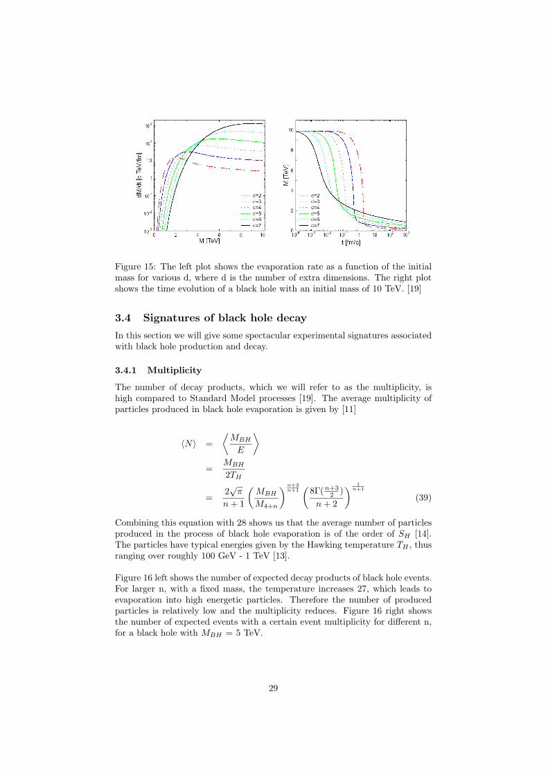
Figure 15: The left plot shows the evaporation rate as a function of the initialmass for various d, where d is the number of extra dimensions. The right plotshows the time evolution of a black hole with an initial mass of 10 TeV. [19]

3.4 Signatures of black hole decay

In this section we will give some spectacular experimental signatures associatedwith black hole production and decay.

3.4.1 Multiplicity

The number of decay products, which we will refer to as the multiplicity, ishigh compared to Standard Model processes [19]. The average multiplicity ofparticles produced in black hole evaporation is given by [11]

〈N〉 =⟨

MBH

E

⟩=

MBH

2TH

=2√

π

n + 1

(MBH

M4+n

)n+2n+1

(8Γ(n+3

2 )n + 2

) 1n+1

(39)

Combining this equation with 28 shows us that the average number of particlesproduced in the process of black hole evaporation is of the order of SH [14].The particles have typical energies given by the Hawking temperature TH , thusranging over roughly 100 GeV - 1 TeV [13].

Figure 16 left shows the number of expected decay products of black hole events.For larger n, with a fixed mass, the temperature increases 27, which leads toevaporation into high energetic particles. Therefore the number of producedparticles is relatively low and the multiplicity reduces. Figure 16 right showsthe number of expected events with a certain event multiplicity for different n,for a black hole with MBH = 5 TeV.

29

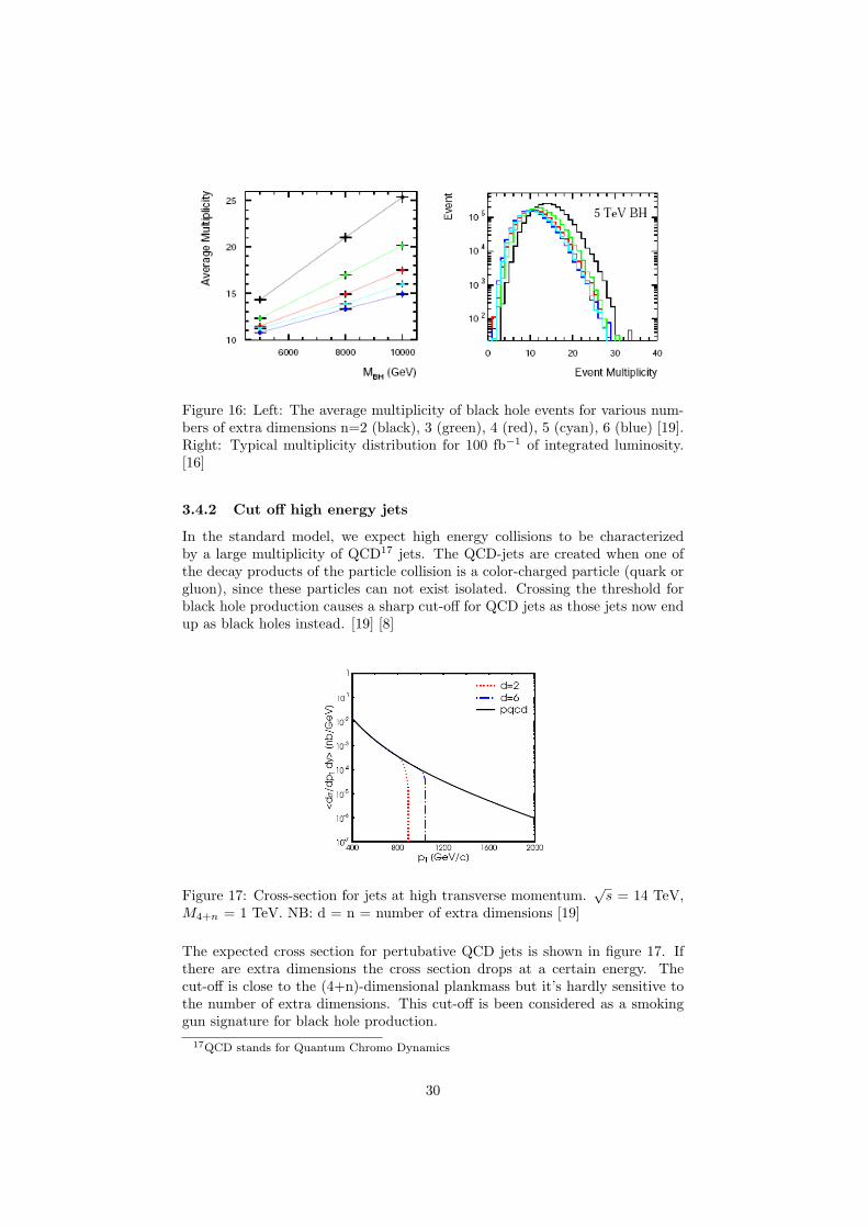
Figure 16: Left: The average multiplicity of black hole events for various num-bers of extra dimensions n=2 (black), 3 (green), 4 (red), 5 (cyan), 6 (blue) [19].Right: Typical multiplicity distribution for 100 fb−1 of integrated luminosity.[16]

3.4.2 Cut off high energy jets

In the standard model, we expect high energy collisions to be characterizedby a large multiplicity of QCD17 jets. The QCD-jets are created when one ofthe decay products of the particle collision is a color-charged particle (quark orgluon), since these particles can not exist isolated. Crossing the threshold forblack hole production causes a sharp cut-off for QCD jets as those jets now endup as black holes instead. [19] [8]

Figure 17: Cross-section for jets at high transverse momentum.√

s = 14 TeV,M4+n = 1 TeV. NB: d = n = number of extra dimensions [19]

The expected cross section for pertubative QCD jets is shown in figure 17. Ifthere are extra dimensions the cross section drops at a certain energy. Thecut-off is close to the (4+n)-dimensional plankmass but it’s hardly sensitive tothe number of extra dimensions. This cut-off is been considered as a smokinggun signature for black hole production.

17QCD stands for Quantum Chromo Dynamics

30

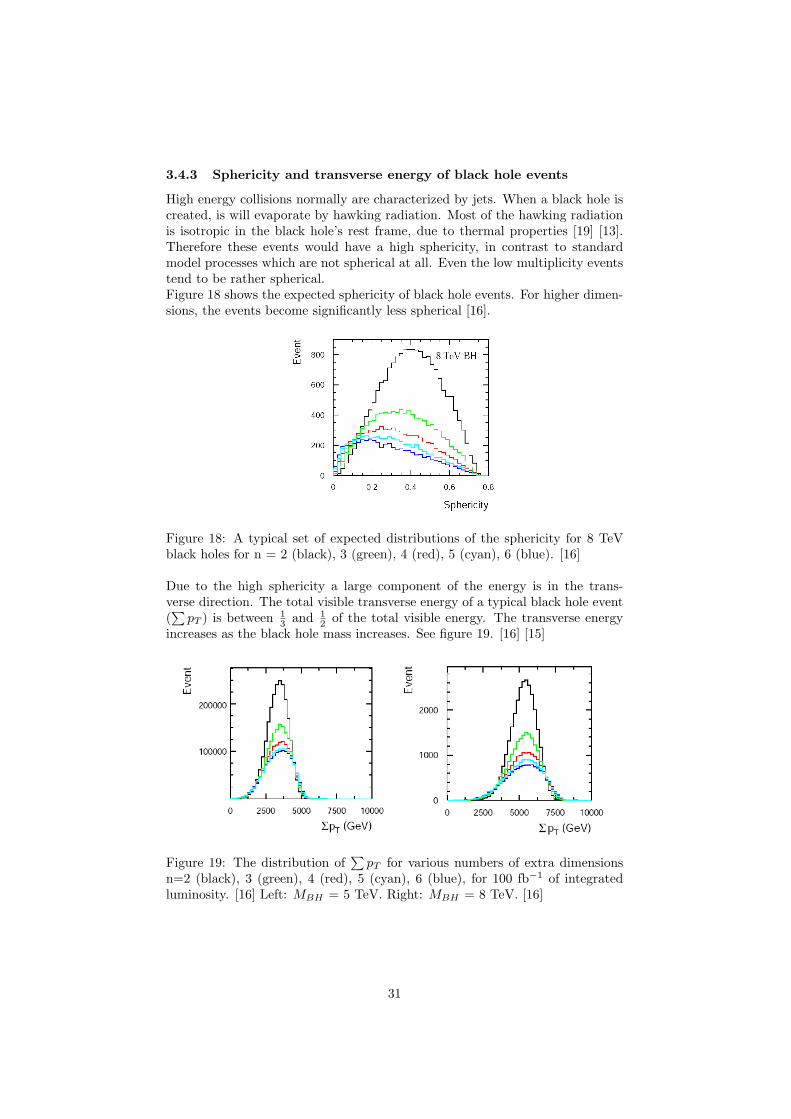
3.4.3 Sphericity and transverse energy of black hole events

High energy collisions normally are characterized by jets. When a black hole iscreated, is will evaporate by hawking radiation. Most of the hawking radiationis isotropic in the black hole’s rest frame, due to thermal properties [19] [13].Therefore these events would have a high sphericity, in contrast to standardmodel processes which are not spherical at all. Even the low multiplicity eventstend to be rather spherical.Figure 18 shows the expected sphericity of black hole events. For higher dimen-sions, the events become significantly less spherical [16].

Figure 18: A typical set of expected distributions of the sphericity for 8 TeVblack holes for n = 2 (black), 3 (green), 4 (red), 5 (cyan), 6 (blue). [16]

Due to the high sphericity a large component of the energy is in the trans-verse direction. The total visible transverse energy of a typical black hole event(∑

pT ) is between 13 and 1

2 of the total visible energy. The transverse energyincreases as the black hole mass increases. See figure 19. [16] [15]

Figure 19: The distribution of∑

pT for various numbers of extra dimensionsn=2 (black), 3 (green), 4 (red), 5 (cyan), 6 (blue), for 100 fb−1 of integratedluminosity. [16] Left: MBH = 5 TeV. Right: MBH = 8 TeV. [16]

31

3.4.4 High missing transverse energy

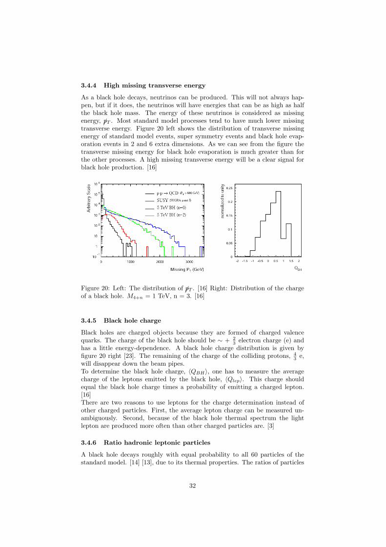
As a black hole decays, neutrinos can be produced. This will not always hap-pen, but if it does, the neutrinos will have energies that can be as high as halfthe black hole mass. The energy of these neutrinos is considered as missingenergy, pT . Most standard model processes tend to have much lower missingtransverse energy. Figure 20 left shows the distribution of transverse missingenergy of standard model events, super symmetry events and black hole evap-oration events in 2 and 6 extra dimensions. As we can see from the figure thetransverse missing energy for black hole evaporation is much greater than forthe other processes. A high missing transverse energy will be a clear signal forblack hole production. [16]

Figure 20: Left: The distribution of pT . [16] Right: Distribution of the chargeof a black hole. M4+n = 1 TeV, n = 3. [16]

3.4.5 Black hole charge

Black holes are charged objects because they are formed of charged valencequarks. The charge of the black hole should be ∼ + 2

3 electron charge (e) andhas a little energy-dependence. A black hole charge distribution is given byfigure 20 right [23]. The remaining of the charge of the colliding protons, 4

3 e,will disappear down the beam pipes.To determine the black hole charge, 〈QBH〉, one has to measure the averagecharge of the leptons emitted by the black hole, 〈Qlep〉. This charge shouldequal the black hole charge times a probability of emitting a charged lepton.[16]There are two reasons to use leptons for the charge determination instead ofother charged particles. First, the average lepton charge can be measured un-ambiguously. Second, because of the black hole thermal spectrum the lightlepton are produced more often than other charged particles are. [3]

3.4.6 Ratio hadronic leptonic particles

A black hole decays roughly with equal probability to all 60 particles of thestandard model. [14] [13], due to its thermal properties. The ratios of particles

32

change a bit due to fact that the particles interact with each other, As well asthe fact that the primary particles decay. The ratio of hadronic and leptonicactivities we will eventually measure is roughly 5:1. This will be a clear signalof black hole decay [15].

4 Conclusion

Within a few years particle physics will possibly make a big breakthrough.Future colliders are going to be able to give particles enough energy to reveal newphysics: mini black holes as well as Kaluza Klein gravitons might be producedand perhaps even detected at these colliders. Whether or not this is going tohappen will decide if extra dimensions, as proposed in the ADD model, existwithin our universe. The existence of these extra spatial dimensions will meanthe end of short distance physics due to the creation of mini black holes at highenergy colliders. On the other hand, it will also mean the beginning of theexploration of the geometry of the extra spatial dimensions.

Acknowledgments

We would like thank Jan de Boer, Nick Jones and Asad Naqvi for their effort,assistance and guidance.

References

[1] http://www.eurekalert.org/features/doe/2003-10/dnal-ftl020904.php.

[2] http://www-cdf.fnal.gov/PES/kkgrav/kkgrav.html.

[3] J. de Boer, N. Jones, A. Naqvi; private communication.

[4] http://scienceworld.wolfram.com/physics/Stefan-BoltzmannLaw.html and http://scienceworld.wolfram.com/physics/PlanckLaw.html.

[5] http://library.thinkquest.org/C007571/english/advance/english.htm.

[6] S. Alexeyev, A. Barrau, G. Boudoul, O. Khovanskaya, and M. Sazhin. Blackhole relics in string gravity: Last stages of hawking radiation. arXiv:hep-th/9906038, January 2002.

[7] Nima Arkani-Hamed, Sava Dimopoulos, and Gia Dvali. The hierarchyproblem and new dimensions at a millimeter. arXiv:hep-ph/9803315, March1998.

[8] Tom Banks and Willy Fischler. A model for high energy scattering inquantum gravity. arXiv:hep-th/9906038, June 1999.

[9] Aurlien Barrau and Julien Grain. The case for mini black holes. CERNcourier, November 2004.

33

[10] Bernard J. Carr and B. Giddings. Quantum black holes. Scientific Amer-ican, April 2005.

[11] Savas Dimopoulos and Greg Landsberg. Black holes at the lhc. arXiv:hep-ph/0412265, June 2001.

[12] O.J.P. Eboli, M.B. Magro, P. Mathews, and P.G. Mercandante. Directsignals for large extra dimensions in the production of fermion pairs atlinear colliders. Physical Review D, 64, July 2001.

[13] Steven B. Giddings. Black holes at accelerators. arXiv:hep-th/0205027,May 2002.

[14] Steven B. Giddings. Black holes in the lab? arXiv:hep-th/0205205, May2002.

[15] Steven B. Giddings and Scott Thomas. High energy colliders as black holefactories: The end of short distance physics. arXiv:hep-ph/0106219, June2002.

[16] C.M Harris, M.J. Palmer, M.A. Parker, P. Richardson, A. Sabetfakhri, andB.R. Webber. Exploring higher dimensional black holes at the large hadroncollider. arXiv:hep-ph/0411022, November 2004.

[17] Steven W. Hawking. The Universe in a Nutshell. Bantan books, 2001.

[18] Stefan Hofmann, Marcus Bleicher, Lars Gerland, Sabine Hossenfelder,Sascha Schwabe, and Horst Stcker. Suppression of high-pt jets as a sig-nal for large extra dimensions and new estimates of lifetime for meta sablemicro black holes - from the early universe to future colliders. arXiv:hep-ph/0111052 v2.

[19] Sabine Hosenfelder. What black holes can teach us. arXiv:hep-ph/0412265,December 2004.

[20] Panagiota Kanti. Black holes in theories with large extra dimensions: areview. arXiv:hep-ph/0402168, December 2004.

[21] G. Landsberg. Collider searches for extra dimensions. arXiv:hep-ex/0412028, December 2004.

[22] Daniel V. Schroeder. An introduction to thermal physics. Addison WesleyLongman Inc., first edition, 2000.

[23] J. Tanaka, T. Yamamura, S. Asai, and J. Kanzaki. Study of black holeswith the atlas detector at het lhc. arXiv:hep-ph/0411095, November 2004.

34