Embed Size (px)
Citation preview
2, g.Q\l
{
Signals in Nonlinear Bandpass Systems
Ian W. Dall, B.E. (Hons.)
Department of Electrical and Electronic EngineeringUniversity of Adelaide
Adelaide, South Australia.
A thesis submitted for the degree of Doctor of Philosophy in:
May 1991
Abstract
Nonlinear tlistortion is a factor limiting performance in many bandpass sys-
tems such as are found in communications and radar. This thesis addresses a
number of theoretical and practical issues relevant to the modelling and correc-
tion of distortion in High Frequency Radar Receivers. The theoretical results
and the experiment methods are applicable to other bandpass systems.
Techniques for modelling nonlinear communication systems, using power se-
ries, amplitude and phase describing functions and Volterra series are reviewed.
Some effort is expended in determining the class of nonlinear systems described
by each model. In many systems, it often the case that only the class of systems
with bandpass input and output is of interest. The usefulness of these models
in predicting the performance of communications systems is evaluated.
It is shown that, for all three models considered, distortion in a bandpass
context can be considered equivalent to distortion of the complex envelope of
signal. It is also shown that the power series model and the amplitude and
phase describing function model are special cases of the Volterra series model.
Many bandpass systems perform a frequency translation function' Radio
receivers invariably use mixers to achieve frequency translation' Mixers are two
input devices and in general the output is a nonlinear functional of both the
input signal and the local oscillator signal. In classical communications receivers
the local oscillator is a sinusoidal function of time, but in applications such as
frequency hopping communications and in radar, the local oscillator may be a
more complex signal.
The number of terms required to model a general, nonlinear functional of
n signals goes up as O(k") so it is undesirable to model a mixer as a general
two input nonlinearity if it is avoidable. Further, modelling a real receiver
Abstract
containing mixers as a general, multi-input nonlinearity would require extra
instrumentation to monitor the local oscillators'
The Wiener model of nonlinear systems is extended to the case of two input
nonlinear systems. This representation is then used to examine the conditions
under which a real mixer can be modelled by a combination of one input nonlin-
earities and ideal mixers. The extended wiener model is also be used to show
that, in a bandpass context, a phase shift in one local oscillator results in the
same phase shift in all the output components'
The discrete time version of the Volterra series is chosen as a suitable means
of modelling and correcting nonlinear distortion, since it is capable of approxi-
mating arbitrarily closely a very large class of nonlinear systems' An adaptive
nonlinear filter based on the discrete time Volterra series is discussed and ex-
tended to the two input case. A number of different adaption algorithms are
discussed and two nonlinear recursive least squares (RLS) algorithms (lattice
and fast Kalman) are derived'
An experiment to estimate nonlinear distortion in an HFR receiver is de-
scribed. There are a number of characteristics which make this experiment
difierent from others described in the literature. specifically:
o The receiver must be modelled as a two input device. The relative phase
of the inputs can not be measured or controlledl'
o The receiver has slight, but important, nonlinear distortion in the presence
of large linear distortion. These two factors place severe constraints on
the adaption algorithms, and prompted the development of the nonlinear
RLS algorithms mentioned above'
o The receiver's inputs and outputs are at different frequencies' This was
lAll the signals are phase locked, but there is no way to set the initial phase
Abstract lll
dealt with by estimating the distortion in the complex envelope instead
of estimating the distortion of the original signals.
¡ The band width of the signals applied to the receiver's inputs should be
very much greater than the band width of the receiver output to ad-
equately probe the front end circuitry. Consequently, it is difficult to
provide enough input samples so that enough information is available in
the output for the estimation to be done. The problem can be alleviated
by sampling the input data at slightly different rates. Different sampling
rates complicates the processing of the data considerably, but the problem
is tractable.
Sufficient experimental results are presented to verify that the methodology
is capable of estimating the receiver's Volterra kernels. The results also verify
some of the theoretical results in the thesis'
It is concluded that more efficient algorithms and/or more powerful com-
puting hardware are necessary before the nonlinear filter approach is a practical
way of estimating or correcting nonlinear distortion in systems similar to the
HFR radar receiver.

Declaration
I hereby declare that this thesis contains no material which has been
accepted for the award of any other degree or diploma in any Univer-
sity, and to the best of the author's knowledge and belief contains no
material previously published or written by another person, except
where due reference is made in the text of the thesis.
The author hereby consents to this thesis being made available
for photocopying and for loans as the University deems fit, should
the thesis be accepted for the award of the degree of Doctor of
Philosophy.
Ian Dall
IV
Acknowledgements
I would like to thank Professor Robert E. Bogner for his effective and con-
scientious supervision of this work. Professor Bogner displayed great patience
and understanding, especially at times when I tended to become side tracked.
His personal library, catalogued and cross referenced in his head, was of im-
mense value. For almost any idea I came up with, he was able to come up with
background reading, often from studies in apparently unrelated areas.
I would also like to acknowledge the financial support of the Australian
Department of Defence through their "Research Scientist Cadetship" scheme'
The High Frequency Radar Division (HFRD), Surveillance Research Labora-
tory (SRL), Defence Science and Technology Organisation (DSTO), provided
technical assistance in the form of equipment and facilities for the experimental
program. Thanks particularly to Mr. Lyndon Durbridge, Mr. Peter Kerr and
Mr. Geoff Warne for their assistance in setting up and operating this equipment.
Thanks also to Dr. Fred Earl, Dr. Malcolm Golley and Dr. Douglas Kewley for
their advice and moral support. Dr. Kewley also proofread the manuscript
which was much appreciated.
Thanks are due to Dr. Richard Stallman, Jim Kingdon and others from the
Free Software Foundation (FSF). The software for the experimental work was
written using gcc which is a C complier from the FSF. Extensive use was made
of. gcc extensions to the C language, which made the numerical code much
Acknowledgements v1
simpler2. Mention should also be made of GNU emacs and gdb, also from the
FSF, which contributed substantially to productive software development. GNU
emacs was used for preparing the manuscript as well as software development'
David Gillespie's calc (a programable calculator package for emacs) proved
valuable for verifying the correctness of C implementations of algorithms.
This thesis was prepared almost entirely using free software. Credit is due
to Professor Donald Knuth (Tbx), Dr. Leslie Lamport (IÂTEX), the MIT X
Consortium (X), Brian Smith (major extensions to xfrg), Thomas Williams
and Colin Kelley (gnuplot), Micah Beck (úransfig), Kevin Coombes (dvi2ps)
and Olin Shivers (cmutex). Contributions to many of these programs were also
made by others too numerous to mention. In many cases, the software needed
modification to meet my requirements which would have been impossible had
the source code not been made freely available by these authors.
Thanks to Mr. Michael Liebelt for cooperation in providing highly accessible
computing facilities, without which it would have been much more difficult to
install all the fore-mentioned software. Thanks also to Mr. Michael Pope for
introducing me to GNU emacs and helping maintain and install many of the
free software packages.
Thanks to Miss Brianna Ferguson for her understanding and emotional sup-
port, even when it seemed I had no time for anything except work and the list of
things postponed until after this thesis was completed appeared to be growing
without limit.
Credit is due to the FESOSA for preserving my sense of perspective and to
the business dinner patrons who helped maintain my sanity. The University of
Adelaide Underwater Hockey Team, Team Trevor and Crabs Canoe Polo teams
maintained my physical health.
2without these extensions, C is rather cumbersome when handling two (or higher) dimen-
sional anays.
Contents
Abstract
Declaration
Acknowledgements
1 Introduction1.1 Definitions
1.1.1 Linearity.
lv
v
1
3
3
3
4
4
1.3 Techniques for Reducing or correcting Nonlinear Distortion 6
1.3.1 Demanding Applications 6
1.3.2 Feedback. 7
1.3.3 Feedforward I1.3.4 Pre or Post Distortion 10
1.3.5 correction by use of Nonlinear Digital Filters (Equalizers) 13
I.1.2 Bandpass Systems
1.1.3 Systems with Memory
1.2 Motivation .
I.4 Outline
L.4.I Signal Dependent Characterization
L.4.2 Parametric Characterization
1.4.3 Multi-input Systems
1.4.4 Nonlinear Digital Filters
1.4.5 HFR Experiments
13
13
I4
15
15
15
vlt
Contents
1.5 Original Contributions
2 Signal Dependent Characterization2.I Introduction
2.2 HarmonicDistortion
2.3 Intermodulation Distortion
2.4 Cross Modulation Distortion
2.5 Polyspectra
2.6 Summary
3 Parametric Characterization
3.1 Introduction
3.2 Instantaneous Distortion
3.3 Amplitude and Phase Describing Functions
3.4 Volterra Series
3.5 The Wiener Model
3.6 Comparison of Models
3.7 Frequency Domain Analysis
3.8 Summary
4 Multi-input Systems
4.1 Introduction . .
vllt
36
36
38
40
42
45
49
50
Ðb
16
20
20
2I
26
30
31
34
57
Ðf
59
61
62
68
69
71.
74
74
lÐ
4.2 A Simplified Model Of Two Input Nonlinearities
4.3 The Wiener Model Of Multi-input Nonlinearities
4.3.1 The Two Input Wiener Model Applied to Mixers
4.3.2 Sinusoidal Local Oscillators
4.4 Phase Transfer
4.5 Summary
5 Nonlinear Digital Filters5.1 Introduction.
5.2 Discrete Time Volterra Series
Contents
Ð.ó
5.4
5.5
b.t)
Nonlinear Adaptive filters
5.3:1 Nonlinear Prediction Estimation and Equalization
5.3.2 Gradient Algorithms
5.3.3 Direct Solution Of the Wiener-Hopf Equations
5.3.4 Recursive Least Squares Algorithms .
Orthogonalization
Multi-input Nonlinear Filters
Implementation Considerations
5.6.1 Initialization
5.6.2 Software
5.7 Summary
6 HFR Receiver Experiments
6.1 Introduction
6.2 The HFR Receiver and Its Operating Conditions
6.3 Design
6.3.1 Equipment. . .
6.3.2 Test Signals
6.3.3 Chirp Generation by Phase Accumulation
6.3.4 Sampling Rates
Analysis Algorithms
6.4.L Complex Envelope Processing
6.4.2 The Ideal Receiver and Sample Interpolation
6.4.3 Adaptive filter Algorithms
1X
77
78
80
85
87
93
94
96
96
96
100
LO2
102
104
105
108
111
1.12
115
t20
t20
t22
t25
128
128
134
L42
t45
6.4
6.5 Results .
6.5.1 Equipment and Procedure Verification
6.5.2 Nonlinear Adaptive Filter Verification
6.5.3 Ëstimation
6.6 Summary
7 Conclusion t49
Contents
A Complex Envelope Equivalent Distortion
B Multidimensional Orthogonal Functions
C Mixers with Sinusoidal Local Oscillators
D Recursive Least Squares Algorithms
D.1 The General Least Squares Problem
D.1.1 Properties of the Transition Matrices
D.2 Time Update Recursions
D.3 The Nonlinear Lattice Filter
D.4 Order Update Recursions
D.4.1 Forward Prediction Coefficient Update
D.4.2 Backward Prediction Coefficient Update
D.5 Error Update
D.6 Auxiliary Variables Update
D.7 Kalman Gain Update
D.8 Gamma Update
D.9 The Generalized Fast Kalman Algorithm
D.10 The Generalized LS Lattice Filter
Bibliography
X
155
158
161
163
165
170
172
176
189
193
20L
206
207
208
212
2t3
215
222
List of Figures
1.1
7.2
1.3
t.4
The bandpass context.
Feedback
Feedforward. .
A piece-wise linear distortion and its inverse.
Harmonic distortion.
IMD intercept point.
The bandpass context
Amplitude and phase describing functions typical of a TWT
The in-phase and quadrature model.
Samples of r(t)The single input Wiener model.
Frequency range of interest for a linear system.
A cube of interest in 3 dimensional frequency space,
A hypothetical system.
A simple model of a mlxer' .
The two input Wiener model
A simple two input non-linearitY.
Phase dependent distortion
The discrete time volterra series
A nonlinear digital filter.
Estimation
3
7
IT2
2.r
2.2
25
28
38
4I
+2
43
46
51
52
54
60
64
7T
72
3.1
3.2
3.3
3.4
3.5
3.6
3.7
3.8
4.L
4.2
4.3
4.4
5.1
5.2
Ð.ó
5.4
lo
76
78
79
xi
Equalization.
List of Figures xll
79
83
84
88
89
91
95
5.5
b.Cr
Ð. I
5.8
5.9
5.10
5.11
6.4
b.Ð
6.6
6.7
Prediction
An error surface with a small eigenvalue spread.
An error surface with a large eigenvalue spread.
Organization of nonlinear terms into column vectors.
Organization of nonlinear terms into column vectors.
Reduced order filter t'taps"
A two input nonlinear filter based on the Volterra series
6.1 Experimental radar receiver block diagram.
6.2 Estimation of a two input receiver
6.3 Approximate estimation of a two input receiver using a single
input estimator. .
Equalization of a two input receiver.
Equipment configuration for HFR receiver experiments.
VHF frequency translator.
Illustration of mixing of aliased components (common sampling
rate).
6.8 Illustration of mixing of aliased components (different sampling
rates).
6.9 Estimation of a two Input receiver
6.10 Illustration of ideal receiver simulation.
6.11 Measured output (doublet LO, triplet RF in).
6.12 Measured output (doublet LO, triplet RF in) omitting start up
transient.
6.13 Simulated output (doublet LO, triplet RF in).
6.14 Measured output ("chirp" LO, noise RF in), omitting start up
transient.
6.15 Measured output ("chirp" LO, noise RF in), omitting start up
transient.
6.16 Measured output ("chirp" LO, noise RF in), omitting start up
107
107
109
110
116
118
t21
t26
1,29
105
106
130
131
r32
i33
transient 134
List of Figures
6.17 Simulated output ("chirp" LO, noise RF i"). . . .
6.18 Simulated output ("chirp" LO, noise RF i"). . . '
6.19 Simulated output ("chirp" LO, noise RF i"). . .
6.20 Comparison of simulated and measured output ("chirp" LO, noise
RF in)
6.21 Receiver gain ("chirp" LO, noise RF in).
6.22 Receiver gain (repeat)("chirp" LO, noise RF in)
6.23 Adaptive filter testing.
6.24 Estimation error due to rounding.
6.25 Estimation error vs number of samples.
6.26 Estimation error vs noise
6.27 Estimation of a pure delay, ì.¡"/Àr : 10-6 ("chirp" LO, noise
RF in)
6.28 Estimation of a pure delay, À-i^/Àr : 10-5 ("chirp" LO, noise
RF in)
6.29 Estimation of the receiver (SVD).
xllt
135
136
r37
138
139
140
141
I4T
L42
143
r44
r45
t46
164
164
178
219
221
D.1
D.2
D.3
D.4
D.5
Organization of nonlinear terms into unequal column vectors. .
Organization of linear terms into unequal column vectors' .
The lattice filter
The generalized lattice filter. .
Reduced generalized lattice filter.
List of Tables
2.1 Third order cross modulation terms
6.1
6.2
Test signal parameters.
Sampling parameters.
D.1 Dimensions of variables.
D.2 f example
113
t20
31
t67
220
xlv
Chapter L
Introduction
As signals are processed by any real equipment, they suffer degradation. The
degradation can be classified as noise or distortion, although the situation is
complicated by noise which also undergoes distortion. Distortion is a determin-
istic process which acts on the input signal(s), whereas noise is an extraneous
signall.
Distortion is such a broad term that little can be said about it unless the
term is qualified. A general distorting system could literally have any output. A
major class of distortion is linear distortion. Linear distortion includes gain and
phase errors. Nonlinear distortion covers everything else. Nonlinear distortion
is still an extremely general term. Indeed, since a nonlinear system might differ
only infinitesimally from a linear system, it can still be said that nonlinear
systems could have any output. In a sense, linear systems can be considered
a special case of nonlinear systems. A linear system is defined in section 1.1.1.
Nonlinear are systems which lack this property. It is not very helpful to define
a class of systems in terms of the properties they lack! To be able to say
l"Noise" is sometimes used to imply a degree of randomness, but "Random Noise" ts a
more correct term in this case.
1
Chapter 7. Introduction
anything useful about the behaviour of nonlinear systems, interesting classes of
nonlinearity must be identified.
One approach is to consider only a class of distortion based on a particular
mathematical form, most commonly the power series. Much of the traditional
work in nonlinear distortion considers the effect of that distortion on a narrow
class of signals (typicalty sinusoids). However, the power series is not capable of
describing nonlinear distortion with memory (see section 1.1'3 for a definition).
The approach taken in this thesis is to concentrate on nonlinearities in band-
pass systems (see section 1.1.2 for a definition). Many practical systems can
be considered to be bandpass. Virtualty all communications, radar, sonar and
electronic warfare systems contain bandpass subsystems. Apart from the band-
pass restriction, the class of nonlinearities considered has been kept as broad as
possible. In particular, nonlinearities with memory are considered.
The experimental work in this thesis has actually been done on an experi-
mental HF Radar Receiver. However, there is little in this work which is not
applicable more widely. Perhaps the most common examples of bandpass sys-
tems are in communications.
This chapter will describe the layout of the rest of the thesis, give an overview
of previous related work and set the context for the authors work. More specific
discussion of previous work is in separate chapters (particularly chapter 2 and
parts of chapters 3 and 5).
2
Chaptet 1. Introduction
L.1- Definitions
1.1.1 Linearity
A linear system is defined as follows: Define !1 and y2 to be the outputs for
inputs of ør and ø2 respectively. The inputs and outputs are typically functions
of time but might also be functions of other independent variables. If the output
is ay1 * byzfor an input of ax1 * bxz, for any l."r,¡ l.,2tand any constant ¿ and ó
then the system is linear.
L.L.2 Bandpass Systems
A nonlinear system in a bandpass context can be considered to be preceded
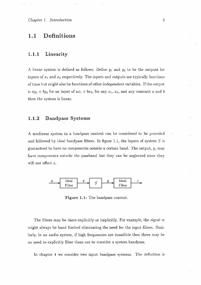
and followed by ideal bandpass filters. In figure 1.1, the inputs of system ,S is
guaranteed to have no components outside a certain band. The output, y, may
have components outside the passband but they can be neglected since they
will not effect z.
3
u t
Figure 1.1: The bandpass context.
The filters may be there explicitly or implicitly. For example, the signal tu
might always be band limited eliminating the need for the input filters. Simi-
larly, in an audio system, if high frequencies are inaudible then there may be
no need to explicitly filter them out to consider a system bandpass.
TIdealFilter ,9
IdealFilter
In chapter 4 we consider two input bandpass systems. The definition is
Chapter 1. Intrcduction
essentially the same as for single input bandpass systems except there is an
implicit filter on each of. the inputs.
L.L.3 Systems with Memory
Nonlinear distortion can be classified as being with or without memory. A
memoryless system is one whose output y(t) at any time ú is a function of its
input r(t) at that same instant. Generally a pure delay can be ignored so that a
system V(t) : f (r(t - ?)) can usually be treated as though it were memoryless.
A system with memory is one whose output at any instant is dependent on the
input at some instants other than the present. Some writers refer to systems
whose memory is short compared to the period of the modulation as being mem-
oryless, which can create confusion2. In this thesis we will refer to systems with
short memory as such, reserving the terms "memoryless" and "zero-memory"
to describe systems whose output can be validly considered to be a function
only of the input at that instant.
L.2 Motivation
The study of nonlinear systems has a long history, but they are none the less
much less well under stood than linear systems. This is partly because they
are inherently more difficult to understand and partly because they have not
received such intcnse attention. In much of engineering practice the assump-
tion of linearity is a good one. Further, the linearity property is a powerful
one in terms of the mathematical manipulations it allows, so there is a strong
temptation to coerce systems into a linear form to make the analysis tractable.
2Note that a truly memoryless system has no phase shift so it is not correct to describe a
TWT, which has amplitude dependent phase shift as "memoryless".
4
Chapter 1. Intrcduction
None the less, there are circumstances where nonlinear characteristics cannot
be ignored, In most systems, there is a requirement that the energy output due
to nonlinear distortion be below some level3. With complex inputs, predicting
the output distortion level is not a trivial exercise. Except for specific inputs
it is not simple to distinguish the nonlinear components of the output from the
linear components, which is necessary lo measure nonlinear distortion. One
approach to determining the distortion output, is to first produce a model and
then use it to simulate the output. This is most useful when it is difficult or
impractical to apply experimental inputs to the original system. Some models
might also be of scientific interest in their own right, especially if they provide
insights into naturai phenomena. Finally, if the levei of nonlinear distortion
components in the output of a system is too high, then steps can be taken to
correct the distortion. We have identified three areas, measurement, modelling
and correction, of nonlinear engineering systems which require understanding.
This thesis contributes to the understanding of modelling and correction. The
measurement problem is discussed in greater detail in chapter 2.
The primary motivation for the work in this thesis was modelling and cor-
recting distortion in High Frequency Radar (HFR) receivers. The method used
has so far proven to be impractical for the particular ðase of the HFR Receiver
because of the amount of computation required. Investigating more efficient
algorithms is a suggested topic for further research. However, a number of the-
oretical results were developed to validate the experimental approach taken.
These results are significant in their own right. See section 1.5 for a more
detailed statement of the contributions made in this thesis.
sThere may also be a requirement on the form that the distortion might take (such as
spectral distribution, energy in a certain band etc)'
5
Chapter 1. Intrcduction
1.3 Techniques for Reducing or Correcting
Nonlinear Distortion
There are a number of known methods for reducing nonlinear distortion. The
simplest is to operate on a more linear portion of the devices characteristic.
Usually that implies operating at a lower power levela. This technique is com-
monly used for microwave Travelling Wave Tube (TWT) amplifiers where it is
known as *back offtt.
1.3.1 Demanding Applications
There are many applications where the linearity of systems is a matter for
concern. Two examples are TWT amplifiers as used in satellite repeaters and
HFR receivers.
"Backing off," a TWT implies that the device is over specified in terms
of power handling capability compared to the case where nonlinear distortion
need not be considered. In the case of satellite repeaters, the weight of a larger
amplifier and its accompanying power supply (such as batteries and solar panels)
is a significant incentive to find other methods of reducing nonlinear distortion.
As more sophisticated modulation schemes are used, the permissible level of
nonlinear distortion goes down.
HFR receivers are another demanding application. Because HF radar op-
erates at a frequency where ionospheric propagation is good, it is subject to
interference from distant HF broadcast stations. Also, like any radar, it may
be subject to deliberate interference (jamming). With this high level of in-
4 "Cross-over" distortion is an exception where operating at a lower level increases the
distortion.
6
Chapter 1. Introduction
terference, it is desirable that nonlinear distortion products be smaller than
the external noise floor so that the minimum detectable cross section is not
degraded.
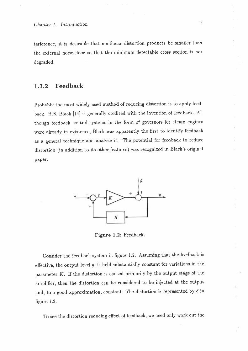
I.3.2 Feedback
Probably the most widely used method of reducing distortion is to apply feed-
back. H.S. Black [1a] is generally credited with the invention of feedback. Al-
though feedback control systems in the form of governors for steam engines
were already in existence, Black was apparently the first to identify feedback
as a general technique and analyze it. The potential for feedback to reduce
distortion (in addition to its other features) was recognized in Black's original
paper.
7
6
+r+ +e
Figure 1.2: Feedback.
Consider the feedback system in figure 1.2. Assuming that the feedback is
efective, the output levely, is held substantially constant for variations in the
parameter I{ . lf the distortion is caused primarily by the output stage of the
amplifier, then the distortion can be considered to be injected at the output
and, to a good approximation, constant. The distortion is represented by ó in
figure 1.2.
To see the distortion reducing effect of feedback, we need only work out the
Chapter 1. Intrcduction
transfer function between the input ó and the output y which is
6Y-t+t<H' (1.1)
The feedback concept contains a causal contradiction. It is an attempt to
correct erroïs after they have happened. This is only effective if the signal e
is essentially unchanged during the time taken for the corresponding feedback
signal to be generated. The applicability of feedback is therefore constrained
by the band width of the loop gain I{ H, the band width of the input signal and
delay in I{ H.
There is, of course, a large body of theoretical and practical knowledge per-
taining to the stability of feedback networks and it is not appropriate to discuss
it here in any detail (some of the significant early advances are documented in
[1a] and [16]). Note, however, that the wider the band width and the greater
the delay, the more difficutt it is to ensure that the feedback network is stable.
The T\MT is a particularly extreme example of a device for which a feedback
network is not usable. Seidel [70] gives approximately 19,000 electrical degrees
as the delay of a particular TWT.
In the Laplace domain, consider the case of. I{H : 10?/(50 * s) which is
representative of a low cost operational amplifier. From equation 1.1, the output
distortion is approximated bY
y(s) æ ó(s)-(-50+s) . G.z)107*s
An interesting feature of this example is that even if ó(t) is due to a "zelo-
memory" distortion, the feedback network as a whole can no longer be consid-
ered to be "zero-memory". Also, there are phase variations due to the zero in
equation 1.2 which would normally be well within the closed loop passband.
8
Chapter 1. Intrcduction
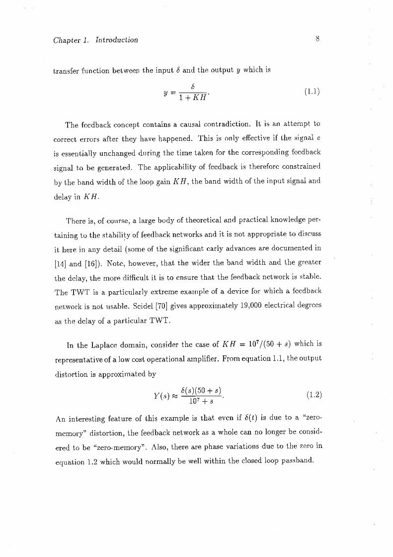
1.3.3 Feedforward
Feedforward is a technique for reducing distortion by detecting errors amplifying
them and injecting them into an appropriately delayed signal in such a way as
to cancel the errors. See figure 1.3. Seidel [70] cites Black [13] as inventing
feedforward in 1924 prior to his invention of feedback. However, the practical
implementation of feedforward networks appears to be pioneered by Seidel [71]
[70].
I
r*6 + r+€
T
-61 r(1 -6+e
Figure 1.3: Feedforward
Unlike the case of feedback, there is no causal contradiction in the concept
of feedforward. In figure 1.3, the time taken for the signal to transit amplifiers
.I(1 and I{2 are explicitly matched by the delays D1 and D2. Assume that the
amplifiers are consist of a pure gain, a pure delay, and an additive error term.
In the case of amplifier .I(r the error is ó. In the case of amplifier -Ifz the error
in the output e includes mismatch between the nominally equal gains Ifi and
Kz.
Provided the individual amplifiers are stable, the feedforward network is
always stable. For the feedforward configuration of figure 1.3 to succeed in re-
ducing distortion, the second amplifier need only have sufficiently low distortion
that e be very much less than ó. It is also necessary that the gain .K2 precisely
match the attenuationlf K1 and that the delay D2 precisely match the delay
+
Chapter 1. Intrcduction 10
in the amplifier Kz. The delay D1 need not match the delay in amplifier .[lr as
closely, but if the match is poor, the amplifier K2 will have to handle a larger
signal than would otherwise be necessary making it more difficult to meet the
requirement that e be very much less than ó.
The chief difficulty with feedforward is the difficulty of matching the delays
D1 and D2 to the delays in the amplifiers K1 and I{2. ln Seidel's work [70], he
used servo controlled electro-mechanical gain and phase controllers. The servo
control loops added significant complexity to the system. If the amplifier delay
is a function of frequency, then the problem of matching the delays in the paths
of the feedforward network becomes even more difficult.
t.3,4 Pre or Post Distortion
Both feedforward and feedback have problems when applied to broad band high
frequency applications. In the case of feedback, the problem is one of maintain-
ing stability and in the case of feedforward the problem is one of matching an
artificial delay to the amplifier characteristics.
There are also situations where neither method is applicable. One such
example is for the correction of distortion in mixers where the output is fre-
quency shifted from the input. Another situation where neither feedback nor
feedforward is applicable is where the input and outputs to the distortion are
not both accessible. For example, it is not possible to use feedback to correct
the distortion in a communication link whether the distortion be due to an ex-
isting repeater, or the transmission medium. Typically, one might be presented
the problem of minimizing distortion over an existing satellite link. Adding
feedforward to existing satellite TWTs is unlikely to be feasible.
In these cases, it may still be possible to correct for distortion by pre-
distorting or post-distorting the signal in such a way as to reduce the over-all
Chapter 1. Introduction 11
distortion. A simple example of such a pre-distortion is shown in figure 1.4.
Schetzen [66], shows that it is always possible to invert distortion represented
as a Volterra series up to the pth order. If the inverse is stable as p -) oo, then
the inverse is exact and the pre-inverse and the post-inverse are the same.
A number reports appear in the literature of attempts to linearize TWT
amplifiers by pre-distortion or post-distortion [20] [37] [64] [36] [65]. Most of
these correction schemes assume that an adequate corrector can be represented
by amplitude and phase describing functions (discussed in section 3.3).
The distortion in figure 1.4 is of the form
(n-
v: I l'-+\,[ å(" - t),
and its inverse is clearly given by
for-l(r(1;for r ) 1;
for c S -1;
U, for -1 <y <I;2V -1, for y ) 1;
2y -I, for y ( -1.
(1.3)
a- (1.4)
In this case the correction is exact and the pre-inverse is exactly the same as
the post inverse. This is not always the case. Some nonlinearities do not have
an inverse. For example the inverse of y - ø2 does not exist because z : xrl2 is
multi-valued. However, even this case can be inverted if r is constrained to be
only positive or only negative. Even where a distortion does not have an exact
inverse, there is still a best approximation to the inverse which can be found.
The optimum pre-inverse and the optimum post inverse are not necessarily the
same [66].
Chapter 1. Inttoduction
v
1
r
Distortion
a
Inverse Distortion
12
1 1
1
1
v11
1
Figure 1.4: A piece-wise linear distortion and its inverse
Chapter 7. Introduction 13
1.3.5 Correction by Use of Nonlinear Digital Filters
(Equalizers)
The method of pre-distortion or post-distortion mentioned in section 1.3.4 ralses
the question of just how can the corrector be implemented. One method which
is capable of optimally correcting nonlinear distortion up to a given order is a
nonlinear digital filter based on the discrete time Volterra Series. This method
is discussed extensively in chapter 5. The problem of setting the coefficients of
such a filter can be handled by adaptive techniques. The implementation and
use of nonlinear adaptive filters is a major part of this thesis. As well as chapter
5 see also sections 6.4.3 and 6.5.2.
L.4 Outline
L.4.L Signal Dependent Characterization
Chapter 2 discusses the way distortion can be characterized in terms of the
distortion products which occur when specific inputs are used. Linear systems
have the property that there are no components in the output at frequencies
which were not present in the input. If the input consists of the sum of a few
sine waves, then any outputs at other frequencies must be due to nonlinear dis-
tortion. Several traditional measures of distortion which take advantage of this
property are discussed. These are ttHarmonic Distortion", "Intermodulation
Distortion" and "Cross Modulation Distortion".
It is observed that these techniques are certainly measures of distortion, but
do not, in general, characterize distortion sufficiently well to enable the output
to be estimated when a more complex input is applied. Nor do these measures
contain enough information to allow a corrector to be constructed.
Chapter 1. Introduction I4
Section 2.5 discusses the application of polyspectra to the observation of
nonlinear distortion products when the input is a Gaussian distributed random
variable. This technique gives a better estimate of how a nonlinear system will
behave with complex inputs.
L.4.2 Parametric Characterization
Chapter 3 discusses models of nonlinear distortion. The signal dependent char-
acterization discussed in chapter 2 are primarily n't,easu,res of distortion, and
are not appropriate for modelling the output of a nonlinear system with a given
input. The measures of distortion can, at least in principle, be used to estimate
the parameters of a model. In chapter 3, bandpass systems are treated by using
a complex envelope represention of the signals.
Section 3.2 discusses instantaneous (memoryless) distortion which can be
represented by a series of functions, most commonly the power series. Sec-
tion 3.3 discusses the amplitude and phase describing function distortion model
which is commonly used to describe distortion in TWTs. Section 3.4 introduces
the Volterra series, a general way of modelling distortion with memory. Sec-
tion 3.5 introduces the Wiener model which separates a general nonlinearity
with memory into a linear, multi-output, linear section followed by a multi-
input, zero-memory, nonlinear section. The power series model, the amplitude
and phase describing function model and the Volterra series model are then
compared by expressing the former two models as special cases of the Volterra
serles.
Section 3.7 provides insights into the nature of bandpass systems by con-
sidering the Fourier transforms of the Volterra kernels. The frequency domain
representation of the power series, amplitude and phase describing functions
and the general Volterra series are considered.
Chapter 1. Introduction 15
L.4.3 Multi-input Systems
The signal in high performance receivers typically goes through two or three
mixers which perform frequency conversion operations. Further, in many mod-
ern communication systems the mixer does not perform a simple frequency
conversion. In radar systems the local oscillator might be a "chirp" (linear fre-
quency sweep) signal. Systems such as this must, in general, be modelled as
multi-input systems.
Chapter 4 addresses the important question of when a two input nonlin-
earity can be represented by a more simple model containing only single input
nonlinearities. Section 4.4 shows that changing the phase of a local oscillator in
a bandpass system changes the phase of .all output components equally. This is
important and desirable behaviour, but it by no means an obvious result.
t.4.4 Nonlinear Digital Filters
Chapter 5 defines the discrete time Volterra series and shows how it can be put
in the form of a nonlinear digital filter. Section 5.3 shows how an adaptive digital
filter can solve the difficult problem of estimating the coefficients of a nonlinear
filter. Applications of adaptive nonlinear digital filters as predictors, estimators
and correctors are also discussed. Sections 5.3.2-5.3.4 discuss algorithms for
estimating the coefficients of an adaptive nonlinear filter. The advantages and
disadvantages of orthogonalization are discussed in section 5.4.
L.4.5 HFR Experiments
Chapter 6 describes experiments performed on HFR receivers which presented
some difficulties in experiment design. Section 6.3 describes the design of the
Chaptet 1. Introduction 16
experiments in terms of equipment, test signal selection and generation and
choice of sampling rates. Section 6.4 describes the techniques used to analyze
the results including calculation of complex envelopes, interpolation to common
sampling rate and the adaptive filter algorithms used for the estimation. Section
6.5 describes the results obtained including steps taken to confirm that the
hardware and software were all working correctly.
L.5 Original Contributions
To the best of the author's knowledge, this thesis makes original contribution
in the following areas.
In chapter 3.2 it is demonstrated that a power series distortion of a bandpass
signal is equivalent to distortion of its complex envelope. This result doesn't
appear explicitly in the literature, but it is a special case of a result by Benedetto
et al [8]. In section 3.6, the Volterra kernels corresponding to the amplitude and
phase describing function model are derived and in section 3.7, by consideration
of the Fourier transform of those kernels, it is shown that amplitude and phase
describing functions are a valid representation of any system if the band width is
narrow enough. It is also shown that frequency independence of the amplitude
and phase describing functions, as measured by a single sinusoid, is a necessary,
but not sufficient, condition for the amplitude and phase describing function
model to be applicable.
In chapter 4, a two input version of the Wiener model is proposed and it
is used to treat a two input nonlinearity as a multi-variable polynomial of the
output of a number of narrowband filters. This model is used to eliminate
components outside the passband and hence it is shown;

Chapter 1. Intrcduction 17
o That a mixer with a sinusoidals input can be modelled as an ideal mixer
cascaded with a single input single output nonlinearity. The nonlinearity,
is however a function of the local oscillator amplitude.
o That a mixer with a broad band local oscillator input can not, in general,
be modelled as an ideal mixer cascaded with a single input single output
nonlinearity.
o That a phase shift in a local oscillator results in a constant phase shift ot
all components within the passband. This is not true when the system is
not bandpass.
In section 5.3.4 (and appendix D which is referenced from section 5.3.4), a
nonlinear filter operating on a scalar is represented as a linear filter operating
on vector quantities {¡ which vary in length. This allows the development of the
nonlinear RLS adaptive lattice filter algorithm and the nonlinear Fast Kalman
algorithm.
As part of the development of the nonlinear RLS algorithms a number of
relationships which are well known for linear systems had to be re-derived for
the "variable length vector" case. These are as follows:
o Derivation of the Wiener-Hopf equations.
¡ Derivation of the definition of the Kalman gain
o Demonstration that there is a (non-adaptive) lattice filter which is the
equivalent of any FIR filter.
o Derivation of an algorithm for converting between the lattice filter and
the transversal filter.
5At least the component within the passband must be sinusoidal. Harmonic distortion of
the local oscillator input has no effect.
Chapter 1, Introduction 18
o For a stationary process, derivation of the relationship between the opti-
mum forward and backward predictor coefficients.
o Demonstration that the optimum forward and backward prediction errors
form an orthogonal basis for the space spanned by the variable length
vectors {¿.
o For a stationary process, derivation of the relationship between the for-
ward and backward partial correlation coefficients I(l^: I<b^- .
In chapter 6, an experimental procedure is developed for nonlinear estima-
tion of an HFR Receiver. There are several characteristics of the HFR Receiver
which required the development of novel techniques' Specifically:
o The receiver must be modelled as a two input device. The phase of the
local oscillator input, relative to the RF input, can not be measured or
controlled6.
o The receiver has slight, but important, nonlinear distortion in the presence
of large linear distortion. The linear distortion is inherent in the high
frequency selectivity of the receiver and implies a long impulse response.
These factors place severe constraints on the adaption algorithms, which
prompted the development of the nonlinear RLS algorithms mentioned
above.
o The receiver's inputs and outputs are at different frequencies. The solu-
tion of this problem by estimating the distortion in the complex envelope
instead of estimating the distortion of the original signals is not new [8].
¡ The band width of the signals applied to the receiver's inputs should be
very much greater than the band width of the receiver output to ade-
quately probe the front end circuitry. Consequently, it is difficult to pro-
vide enough input samples so that enough information is available in the
6All the signals are phase locked, but there is no way to set the initial phase.

Chapter 1. Introduction 19
output for the estimation to be done. The problem can be alleviated by
sampling the data for the two inputs at slightly different sampling rates.
Experimental evidence is presented to support the theoretical result derived
in section 4.4 where where it was shown that a constant phase shift of a local
oscillator, results in a constant phase shift of all the components (linear and
nonlinear) in the passband.
Chapter 2
Signal Dependent
Charact erization
2.L Introduction
Traditionally, distortion has often been characterized by its effect on an input
consisting of one or more sinusoids. This leads to terms such as "Harmonic
Distortion" and "Intermodulation Distortion". These are indeed measures of
distortion, but they do not in themselves constitute identification of a nonlinear
system. For example, it is not possible to know what the output of a system
with a% harmonic distortion will be for any input other than a sine wave of the
same amplitude and frequency as the original test. However, with enough such
measurements, it is possible under certain constrainis, to derive an estimation
of a nonlinear system. The more general the model, the more measurements are
required. If one has an adequate parametric characterization (a model), it is
relatively easy to predict the signal dependent characterization. Unfortunately
the reverse is not generally true.
The distortion characterizations based on sinusoids (sections 2.2-2.4) arc
20
Chapter 2. Signal Dependent Charactetization 2t
quite old and are covered here chiefly as a contrast to the Parametric Models
introduced in chapter 3. Signal dependent characterization (notably Intermod-
ulation Distortion and Harmonic Distortion) is used by most manufacturers in
specifying the linearity of their devices. The application of polyspectra (section
2.5) to the characterization of nonlinear systems is much newer and, to the
authors knowledge, no manufacturers specify linearity in terms of polyspectra,
although it might make sense to do so.
To understand the signal dependent characterizations of sections 2.2-2.4, we
will examine the output of a power series with various inputs. The power series
is the simplest commonly used parametric model of distortion. To an extent we
are pre-empting chapter 3, but the power series is simple enough to need little
introduction.
2.2 Flarmonic Distortion
It is not clear when harmonic distortion was first theoretically predicted.
Since second harmonic distortion arises fairly directly from the "double angle"
trigonometric identities the concept is undoubtedly quite old' Richards [58]
traces the theory of suó-harmonics (which only arise in systems with memory)
to Mathieu in 18681, so it would be surprising if the generation of harmonics
where not understood well before this. Some treatment of harmonic distortion
can be found in text books by Panter [55] and Calson [19].
There are several approaches which can be taken to demonstrate the gener-
ation of harmonics by a nonlinear system. First, consider a power series
n
a(t) :la¿x(t)i.i=1
lSub-harmonics where obserueil as early as 1831 by Faraday
(2.1)
Chapter 2. Signal Dependent Chanctetization 22
Now we can represent a sinusoidai input by
r(t): cos(øsú), (2'2)
and by the use of trigonometric identities we can show the production of har-
monics. For example, in the case of the term n :2 in equation 2.1.,
11r(t)2 : i* ¡cos(2øsú). (2.3)
Alternatively, we can Ieplesent the sinusoidal input as a sum of complex expo-
nentials,
r(t): Acos(øsú + do)A2
(ei,ot+öo + e-i'ot-Ao) (2 4)
This tends to be easier to handle, especially for higher powers of n or when
óo#0.
r(t) : (ei,or+oo + e- i'ot-ôo)"
"i @ - í) (uot I óo)
"- i i(uot + óo)
"i(n-2i)(,'tottöo) . ( 2.5)
If we now note that the ith term has the same magnitude centre frequency as
the /th term if n -2i: -(n -2t) \.e. I -- n - i, then we can group the terms
in equation 2.5 in pairs. The expansion now takes a slightly different form if n
is even or odd. For n odd
(+)"
(+)"
(+)"
)/2-1x(t)^: (+)"'
)" (:,,) * (+)"'"
ti=0 "i(n-2i)(uotlöo)
¡ "-i(n-2i)(uotlóo)n
n-i(2.6)
and for n even
.Q): (+ [(î) """-'i)(øst+óo)
l2)-Di=0
- j(n-2á)(uot+óo)
(2.7)
Chapter 2. Signal Dependent Chancterization
Now we use the fact that (;) : ('i) ,. simplify equations 2.6 and 2'?' For n
23
odd,
and for r¿ even,
x(t)^ : (+)"'-Ë^'' (î) ".'((' - 2i)(ust* do)) , (2.8)
r(t)' : (+)" (:,r). (+) (î) ".. ((, - 2i)(ust+ do)). (2.e)n (n/2)-t.
Di=0
It is worth observing that a common short cut when dealing with linear
systems is to represent a sinusoid by ei'ot+öo, effectively forgetting about the
negative frequency component of equation 2.4. If the signal is to go through a
nonlinear process, this simpler representation does not give the correct result.
Instead of equation 2.5 we would simply have r(ú)" - ft¿jn(c'rot+do) which would
correctly predict only one of the components in equations 2.8 and 2.9.
Yet a third method of determining the components of a power series of a
sinusoid is to perform the manipulations in the frequency domain. We note that
multiplication in the time domain is equivalent to convolution in the frequency
domain. Also, a sinusoid has a very simple representation in the frequency
domain as two delta functions. The final factor which makes this approach at-
tractive is that the convolution of a function with a delta function is particularly
easy to do,
X(r) * ó(cu - ,o): X(ø - ,o). (2.10)
The method is less attractive when an arbitrary phase shift must be incorpo-
rated. If
x(t) : cos(cu6ú)
then
x(r) : Lr(.d{,-,o) + 6(,+ ro))
F(x(t)2): X(a) * X(u)
: (;)' 6(, - 2,o) + 26(u)* ó(a, * 2us))
and higher orders can be handled by recursion
Chapter 2. Signal Dependent Characteilzation
F(x(t)") -- F(x(t)-l) * X(ø) (2.11)
This method is intuitively satisfying, especially to someone with a familiarity
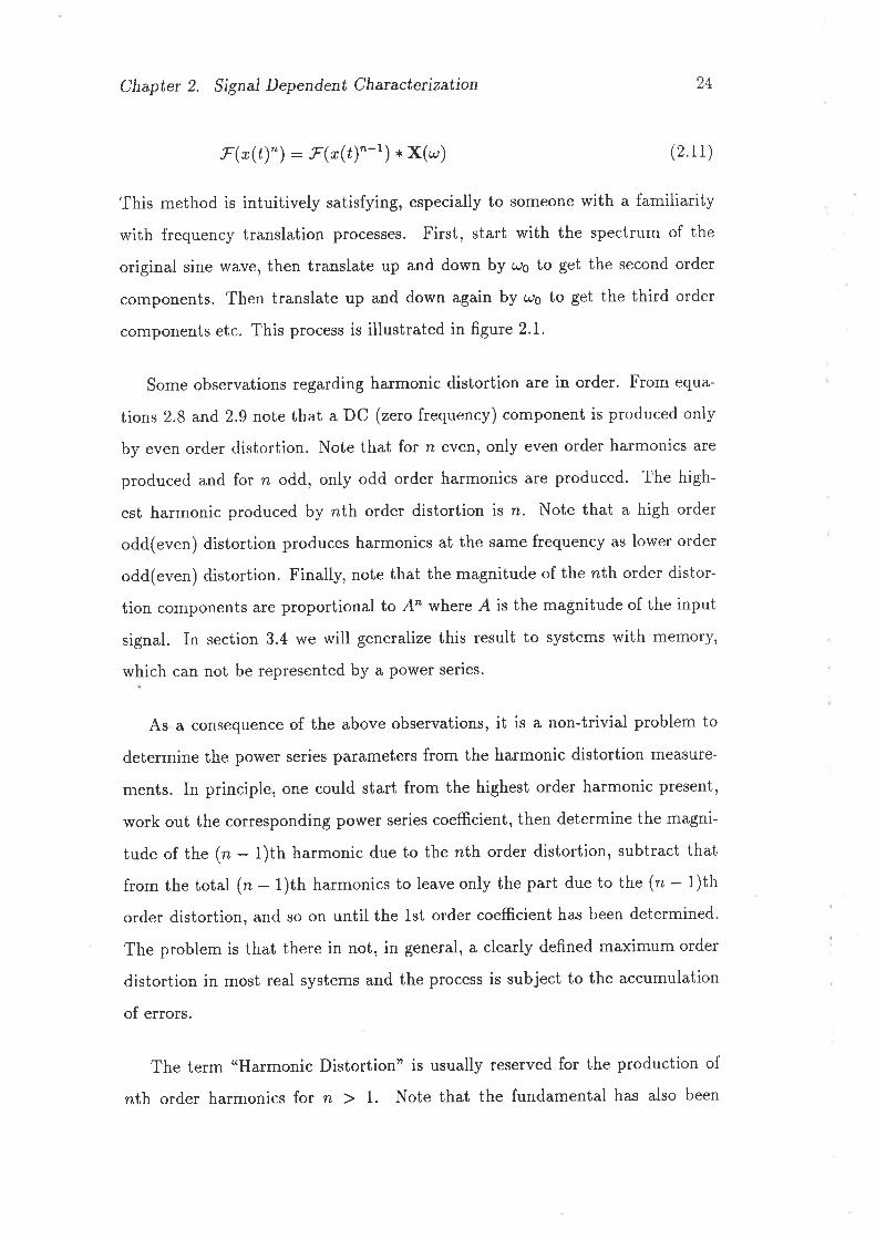
with frequency translation processes. First, start with the spectrum of the
original sine wave, then translate up and down by ,o to get the second order
components. Then translate up and down again by ,o to get the third order
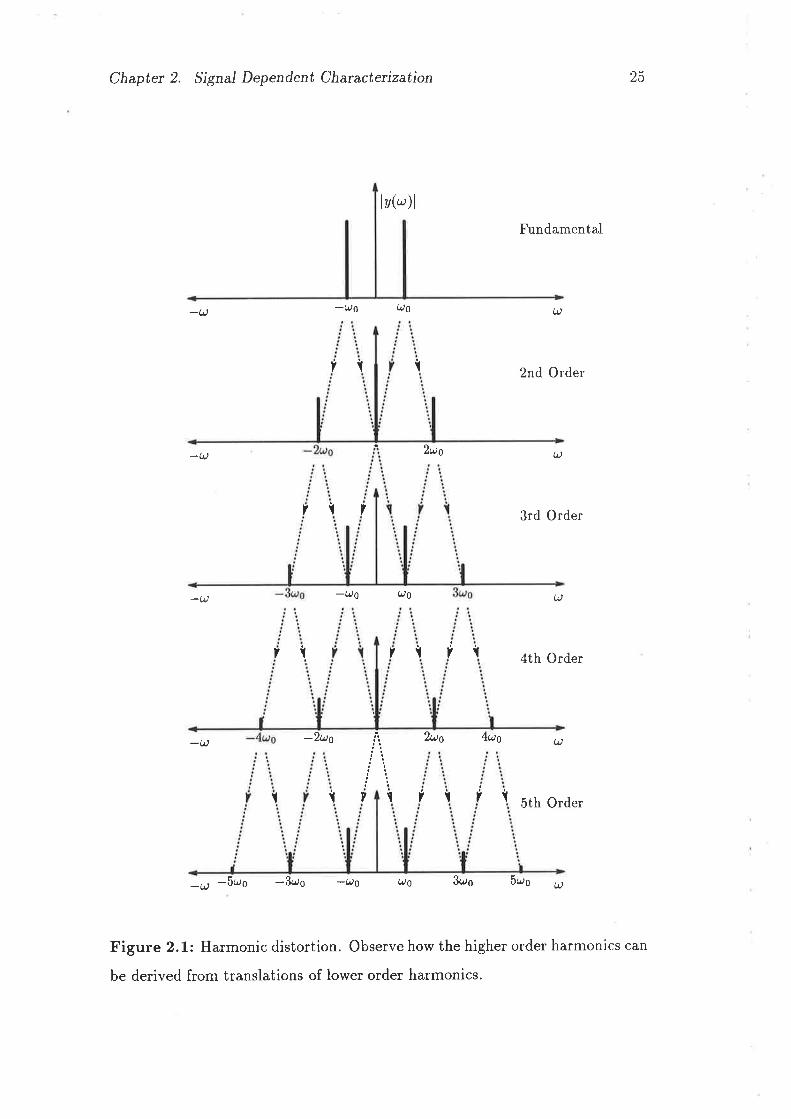
components etc. This process is illustrated in figure 2.1.
Some observations regarding harmonic distortion are in order. From equa-
tions 2.8 and 2.9 note that a DC (zero frequency) component is produced only
by even order distortion. Note that for n even, only even order harmonics are
produced and for n odd, only odd order harmonics are produced. The high-
est harmonic produced by nth order distortion is n. Note that a high order
odd(even) distortion produces harmonics at the same frequency as lower order
odd(even) distortion. Finally, note that the magnitude of the nth order distor-
tion components are ptoportional to A" where A is the magnitude of the input
signal. In section 3.4 we will generalize this result to systems with memory,
which can not be represented by a power series.
As a consequence of the above observations, it is a non-trivial problem to
determine the power series parameters from the harmonic distortion measure-
ments. In principle, one could start from the highest order harmonic present,
work out the corresponding power series coefficient, then determine the magni-
tude of the (n - 1)th harmonic due to the nth order distortion, subtract that
from the total (n - l)th harmonics to leave only the part due to the (n - 1)th
order distortion, and so on until the 1st order coefficient has been determined'
The problem is that there in not, in general, a clearly defined maximum order
distortion in most real systems and the process is subject to the accumulation
of errors.
The term "Harmonic Distortion" is usually reserved for the production of
nth order harmonics for r¿ ) 1. Note that the fundamental has also been
24
Chapter 2. Signal Dependent Chancterization
ls(r)l
-u -UO QO
25
iit
u0 3øo
Fundamental
2nd Order
3rd Order
4th Order
O)
5th Order
u
u
u2uo
(t
-u
,
iI I
-u0 uO-u
7l rl t t
-2uo 2uo 4uo-u
tI I iI t I
-a -5ro -3øo -uo 5øo
Figure 2.1: Harmonic distortion. Observe how the higher order harmonics can
be derived from translations of lower order harmonics.
Chapter 2. Signal Dependent Chaructetization 26
distorted because higher odd order distortion produces components at the fun-
damental frequency. The amplitude of the fundamental is no longer linearly
related to to the amplitude of the input' This is one form of "in-band" dis-
tortion, a term which arises when considering bandpass systems where higher
order harmonics are outside the systems passband'
This nonlinear relation between the input amplitude and the amplitude of
the fundamental, or the amplitude of a higher order harmonic, can be exploited
to identify the coefficients of the power series [53][12]'
2.g Intermodulation Distortion
we saw, in the case of harmonic distortion, that we couid view harmonic dis-
tortion as a sine wave translated n times by it's own frequency' The method
is summarized equations 2.10-2.11 and figure 2.1. when the input consists of
components at more than one frequency, we have the case where components at
one frequency are translated by a difterent frequency resulting in components at
sums and differences of the original frequencies. These components are known
as Intermodulation Distortion (IMD) products'
It is difficult to trace the first theoretical prediction of the phenomenon of
intermodulation distortion. Like harmonic distortion, the existence of inter-
modulation distortion can be predicted fairly directly from basic trigonometric
identities. certainly intermodulation distortion was of concern by 1934 when
Black wrote his paper on feedback [14], since he cites reduction of "modulation
products,, in muiti-channel telephone systems as a major feature of feedback'
Intermodulation distortion is treated in some depth in a text book by Panter
[56].
To see how intermodulation terms arise, consider the case of a two tone
Chapter 2. Signal Dependent Chatacteñzation
input into a system described by the same power series (equation 2'1)' If the
input is
r(t):A(cos(ø1ú) *cos(ur2ú)) (2.12)
then the nth term in the power series is given by
r(t\n:A"i 11).o."-n(ø1ú)cos;(ø2ú). (2.t3)'-\ / ã \, /In the treatment of harmonic distortion (section 2.2), we derived expansions for
cos'(ø¡ú) which can be substituted into equation 2.13. However, the expression
becomes complicated and does not provide great insight' Instead consider the
particuiar case of n :3,
r(t)3 : A3 (cos3(tr1¿) + 3 cos2(t,l1ú) cosl(ur2f )
* 3 cosl (c,'r1ú) cos2(ø2t) + cos3(øzÚ))'(2.r4)
The cos3 terms give rise to harmonic distortion but the remaining terms give
rise to Intermodulation Distortion components.at ø - 2at - a2 and u :2uz -u1. Since equation 2.13 contains terms which correspond to both harmonic
distortion and intermodulation distortion, it is apparent that the occurance of
these components is more a feature of the input than of the nonlinear system'
All the components of equation 2.14 increase in proportion to 43. Calculation
of ail the IMD terms for high orders or for many input tones can be readily
performed numerically [69].
As with the case of harmonic distortion, different order IMD components
may have the same frequency. For example, there are fifth order components
at2L,t_uz*Qz_uzwhicharethesamefrequencyasthe2u¡_t¿zthirdordercomponent. The fifth order component increases in proportion to A5 and the
third order component increases in proportion to 43. For small A, the frequency
component will increase as if it were a third order system and for a larger A it
will increase as if it were a fifth order system. If plotted on a logarithmic scale,
the amplitude of the distortion component as a function of the input amplitude
27
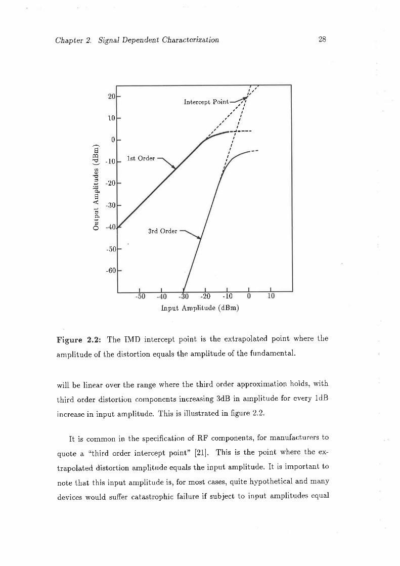
Chapter 2. Signal Dependent Chancterization 28
10
-10
20
-50
-20 -10
Input Amplitude (dBm)
Figure 2.2: The IMD intercept point is the extrapolated point where the
amplitude of the distortion equals the amplitude of the fundamental.
will be linear over the range where the third order approximation holds, with
third order distortion components increasing 3dB in amplitude for every 1dB
increase in input amplitude. This is illustrated in figure 2.2.
It is common in the specification of RF components, for manufacturers to
quote a "third order intercept point" [21]. This is the point where the ex-
trapolated distortion amplitude equals the input amplitude. It is important to
note that this input amplitude is, for most cases, quite hypothetical and many
devices would suffer catastrophic failure if subject to input amplitudes equal
0
30
4
t{
Øq)
ÈH
€
-60
1st Order
3rd Order
Intercept Point tI
,,J,
,t
tt
Chapter 2. Signal Dependent Chamcteñzation 29
to the IMD intercept value. The advantage of specifying the performance this
way is that it is quite easy to work backwards using the rule of 3dB change in
distortion level per ldB change in input level to the operating point actually
used.
It is possible to analyze Intermodulation Distortion with distortion models
other than the pov¡er series [10] [72] [63] [43] [73] [50] [49] [56]. The nonlinearities
in microwave communication systems are often described using amplitude and
phase describing functions. These systems are often Frequency Division Multi-
ple Access (FDMA) and it is of interest to know how intermodulation distortion
between channels interfere with other channels. Analysis of such systems can
become quite complex due to the number of channels, although simplifications
can be made if it is assumed that the distortion is only of low order (eg third
order only). The simplest such analysis considers only the (sinusoidal) carriers
of each channel but some analysis which assumes simple modulation has been
performed [10] [72] [63] [43] [73] [56]. Analysis of system performance with more
accurate representations of the input has been performed numerically [30].
The term Intermodulation, rather implies an effect between two or more
separate signals. Of course, any input can be approximated arbitrarily well as
a sum of sinusoids (effectively performing a Fourier Transform), and the distor-
tion can, at least in principle, be determined by considering the intermodulation
between all the sinusoids. Whilst this is a perfectly valid method of analysis,
the author doubts whether "Intermodulation Distortion" is the most appropri-
ate term to apply to such a system. When considering the cumulative effect
of all the different order intermodulation products arising from all the input
components, the phase of the distortion products must be taken into account.
The commonly measured "IMD Intercept Point" contains no information on
the phase of the resulting components.
Chapter 2. Signal Dependent Chancterization 30
2.4 Cross Modulation Distortion
When a modulated carrier is passed through a nonlinear system with another
carrier (modulated or not), the modulation of the first signal is transferred (a1-
beit distorted) to the second carrier. This is termed cross modulation distortion.
It is difficult to trace the first theoretical prediction of the phenomenon
of cross modulation distortion. One of the most interesting manifestations of
cross-modulation distortion is due to nonlinear ionospheric propagation. This
was first observed by Tellegen in 1933 [74] when it was observed that the Lux-
embourg radio station (252kHz) could be heard on a radio tuned to a signal
from Beromünster (652kHz). The phenomenon has come to be known as the
Luxembourg effect. Cross-modulation in electronic circuits must have already
been known since Tellegen rules this out (on the basis of field strengths) as the
cause of his observations. For a discussion of the mechanism of distortion in
ionospheric propagation see the text by Budden [18].
To see how cross-modulation can happen, consider an input with the fre-
quency domain representation
X(r) : atl6(u - rt) f 6(u+ ør)l
* a2l6(u - (r, - Ar)) * ó(ar * (r, - Ar))l
* ø3 [ó(ø - ,r) * 6(cu + ,r)]
* aaf6(u - (r, + Aø)) I 6(a * (r, + Aø))l . (2.15)
This is a representation of an unmodulated signal at a frequency of ar1 and a
carrier at a frequency of ø2 with two modulation sidebands at frequencies of
uz * L,a and ø2 - L,u. This could represent AM modulation with a frequency
of Ac,.r. By choice of. a2, d3 and øa, AM, SSB and DSB could be represented.
Other modulation schemes also contribute to cross modulation distortion, but
they aren't easily incorporated in this simple analysis. Note that there is no
difference mathematically between a number of independent sine waves and
Chapter 2. Signal Dependent Characteilzation 31
a single modulated carrier. The only difference is that a decoder (or human
listener) might interpret information in the transferred modulation. In that
sense, cross modulation distortion is in the ear of the beholder!
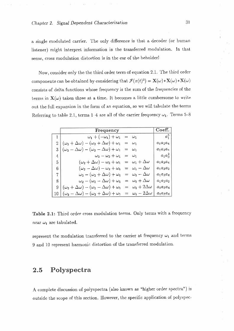
Now, consider only the the third order term of equation 2.1. The third order
components can be obtained by considering that F(r(t)3): X(ø)*X(ø)*X(ø)consists of delta functions whose frequency is the sum of the frequencies of the
terms in X(cu) taken three at a time. It becomes a little cumbersome to write
out the full expansion in the form of an equation, so we will tabulate the terms
Referring to table 2.1, terms 1-4 are all of the carrier frequency cl1. Terms 5-8
Frequency Coeff.1
2
3
4
b
6
I
8
9
10
ør*(-ør) +ør(rr+ar) -(rr+aø) *ør(rr- Ar) - (rr- Aø) *ør
u2-Q2!a1(rr+Ar) -uz*ut(rr-Ar) -uz*utuz-(uz1 Aø) *øruz-(uz-Aø) *ør
(rr+ ar) - (rr- aø) *ør(rr- Ar) - (rr+At;) *c.rr
:41w7
:U1:U1: IÐ1
:U1wl
:Q1wlw7
*Aø-Aø- L,a*Aø* 2L,u
- 2A,a
ald1A2o,4
A1o,2CI4
ap2z
&10,sCL4
CIlAgd2
A1A3O,4
0,1fI34,2
A1Agd4
Ay04CI4
Table 2.1: Third order cross modulation terms. Only terms with a frequency
reâ,r ûJ1 are tabulated.
represent the modulation transferred to the carrier at frequencY Qt and terms
9 and 10 represent harmonic distortion of the transferred modulation.
2.5 Polyspectra
A complete discussion of polyspectra (also known as "higher order spectra") is
outside the scope of this section. However, the specific application of polyspec-
Chapter 2. Signal Dependent Characterization 32
tra to the observation of nonlinear phenomena will be briefly discussed
In the previous sections of this chapter, we have seen that nonlinear dis-
tortion results in components in the output at frequencies which may not be
present in the input. In the case of a noisy output, there may be a sponta-
neously generated component at the same frequency as the distortion product'
The component due to nonlinear distortion bears a definite phase relationship
to the input of the nonlinearity whereas the spontaneously generated compo-
nent will be uncorrelated to the input of the nonlinearity. Polyspectra provide
a way of differentiating between these components. A most convenient way of
observing the nonlineal components is to select the input in such a way that
the polyspectra of order greater than 2 aÍe zelo if the system is linear' Then
any non-zero polyspectra of order greater than 2 must be due to nonlinearities.
It is sufficient that the input be a Gaussian random process.
Polyspectra are defined in the literature [45] [54], as follows. First, define
the joint moment generating function of the set of n real random variables,
{*tr,rr"',rr,},bYO(',, u)2¡ " ' ,un) : t(el@"t+'2a2*"'*øntn)¡' (2'16)
Equation 2.16 is also known as the joint characteristic function. The term
"moment generating function" arises since the moments are given by
ffikt,...,r,n = t(xf'*t' '''"Y)ô'Q(utru2,¡ . .. , @") I:(-J)'ffi1"="=,='n=o
(2.t7)
(2.18)
where
r:lq*kz*...+1e,.
Bquation 2.18 can be readily verified by substituting equation 2.16 into equation
2.18 and exchanging the order of the expectation and differentiation operations.
The joint cumulants are then defined
, .\, }'IogQ(rr, t¿)2t . . ', ør) I /t 1 o\ckt"'kn = (-l) @l.r=rr=,.._rn_o \4'L¿t
Chapter 2. Signal Dependent Charucterization 33
The definitions 2.16 to 2.19 are straight forward extensions of equivalent func-
tions of a single random variable [76] [57].
Now consider a real stationary random process
{x(fr)}, k - ...,-2,-1,0,L,2,...
and define
civ(rr ,T2r, ,. , zrv-r) = cxlx¡,x1t *r),x(k¡r2),...,x(,b*rrv-r)' (2'20)
Equation 2.20 is for the discrete case with ri - ...,-2,-1,0, I,2,.' '. This def-
inition follows the notation of Nikias and Raghuveer [5+] although they appear
to have omitted the actual definition from their paper. Finally the l/th order
spectrum is defined as the N - I dimensional Fourier Transform of equation
2.20. Bendat [6], defines higher order spectra as the Fourier transform of higher
order auto-correlation functions which is the same as the moment of the ran-
dom variables X(,t), X(k+r1),X(k+r2),...,X(k * ¡¡¡-r). In short, Bendat
[6], defines higher order spectra as the Fourier transform of the moment, rather
than the Fourier transform of the cumulant. It happens that these definitions
are the same for N < 3 but differ for N > 3 [54].
Some properties of polyspectra are:
1. The second order spectrum is the familiar power spectrum [54].
2. For a Gaussian process, the nth order spectrum is zero for n à 3 [54] [45].
3. The bispectrum B(rt,ø2) represents the correlation of the component at
a frequency or * cu2 with the product of the components at frequencies of
ûr1 and u21541.
As a consequence of the above properties, polyspectra provide no extra
information if a Gaussian input is applied to a linear system. However, with a
Chapter 2. Signal Dependent Characterization 34
non-Gaussian random input, it is possible to identify a linear system [54] [34] [75]
[35]. With only the power spectrum it is possible to identify the magnitude of a
systems transfer function, but not it's phase. Further, if the input is Gaussian
and the higher order spectra for n ) 2 are not zero, then the system must be
nonlinear and property 3 (above) gives a reasonably intuitive interpretation.
Linear system identification using polyspectra has the advantage that the
actual input does not need to be known, however, where the input is known (or
measurable), then methods using polyspectra are unlikely to ever compete with
more traditional methods. Without attempting a rigorous analysis (which could
be made obsolete by more efficient methods) we simply observe that discarding
the input information is unlikely to make the identification task easier. At the
time of writing, it does not appear possible to identify a general nonlinearity
using polyspectra2.
2.6 Summary
In this chapter we have examined three traditional measures of distortion, "Har-
monic Distortion", t'Intermodulation Distortiont' and "Ctoss Modulation Dis-
tortion". These names suggest that the distortions are somehow different, but
these effects can occur from the same nonlinearity, the only thing to change
being the complexity of the input signal. If the input consists of only a single
sinusoid, then we only see harmonic distortion. If the input has two sinusoids
then we see intermodulation distortion as well as harmonic distortion. If the
system consists of more than two sinusoids and we consider one of them to be a
modulation sideband then we can observe cross modulation distortion in addi-
2There does not appear to be any cases in the literature of nonlinear identification using
solely (auto)-polyspectra. However, cross-polyspectra (of input and output) have been used
for system identification [44] [i]. The method can be applied to systems distributed in space
as well as time [59].
Chapter 2. Signal Dependent Characteúzation 35
tion to harmonic distortion and intermodulation distortion. Note that when the
distortion products from different input components have the same frequency,
then the phase of the products must be taken into account when working out
the cumulative effect.
Polyspectra (or higher order spectra) provide a rvvay of detecting nonlinear
distortion when the input is an unknown Gaussian process'
These terms "Harmonic Distortion", "Intermodulation Distortion", "Cross
Modulation Distortion" and "Polyspectra" (when the input is Gaussian), are
similar to the extent that they are all rneasures of distortion, but they are not
models of distortion. None of these methods are suitable for predicting the
output of a system with a different input (which is the prime purpose of a
model).
As has been mentioned, it is possible to use these measures of distortion
to evaluate the parameters of a model although, as we will see in chapter 3, a
general model can not be evaluated with simple inputs consisting of only a few
sinusoids.
Chapter 3
Parametric Charact erization
3.1. Introduction
Most of the work in this chapter was covered in a paper by myself and Bogner
[2a]. Signal degradation may be due to noise or to distortion. Linear distortion
may be caused by filters, dispersion or multipath effects. These effects are well
understood and can often be minimized by linear equalizers. To make further
improvements it is necessary to consider the correction of nonlinear distortion.
Distortion correction can be performed by using pre or post distortion to com-
pensate ([5] , [8] [28], [63], [64] and [68]). It is desirable to know whether the
structure chosen for a distortion compensator is capable of correcting a partic-
ular class of distortion. To this end it is necessary to have a valid model of
the distortion to be corrected. The model must be able to simulate the out-
put quite accurately. This application is more demanding than some where a
reasonable estimate of the magnitude of the distortion may be all that is re-
quired. For example, harmonic distortion measurements and intermodulation
distortion measurements discussed in chapter 2 give an estimate of how severe
the nonlinearity is (and even that may be inaccurate) but are quite unsuitable
for predicting the form of the distortion.
36
Chapter 3. Parametric Chancterization 37
Nonlinear distortion can be classified as being with or without memory. A
memoryless system is one whose output y(t) at any time ú is a function of its
input r(ú) at that same instant. Generally a pure delay can be ignored so that
a system y(t): f @(t - ")) can usually be treated as though it were memory-
less. A system with memory is one whose output at any instant is dependent
on the input at some instants other than the present. Some writers refer to
systems whose memory is short compared to the period of the modulation as
being memoryless, which can create confusion. In this chapter we will refer
to systems with short memory as such, reserving the terms "memoryless" and
"zero-memory" to describe systems whose output can be validly considered to
be a function only of the input at that instant.
Many of the physical phenomena causing nonlinearities are essentially mem-
oryless but they are often embedded in a network of linear components which
cause the component as a whole to have memory. Further, virtually all com-
munication systems have filters intentionally included to reduce susceptibility
to thermal noise in receivers and to reduce out of band spectral emissions. De-
tailed discussion of the design of these components is not appropriate in this
chapter, but in general terms the band width of the filters will be a compromise
between reducing thermal noise and reducing intersymbol interference. Conse-
quently it is unlikely that practical communication system nonlinearities can be
adequately modelled as memoryless.
In this chapter we will first review some established methods of modelling
distortion. These are, in order of increasing generality, infinite series of functions
(such as power series), amplitude and phase describing functions, the Volterra
series and the Wiener model. These have all been used extensively in the
literature but the question of under what circumstances the less general models
may be adequate has been largely ignored. We will attempt to redress this
balance by comparing the less general models with the Volterra series model of
the same system.
IdealFilter^9r
IdealFilter
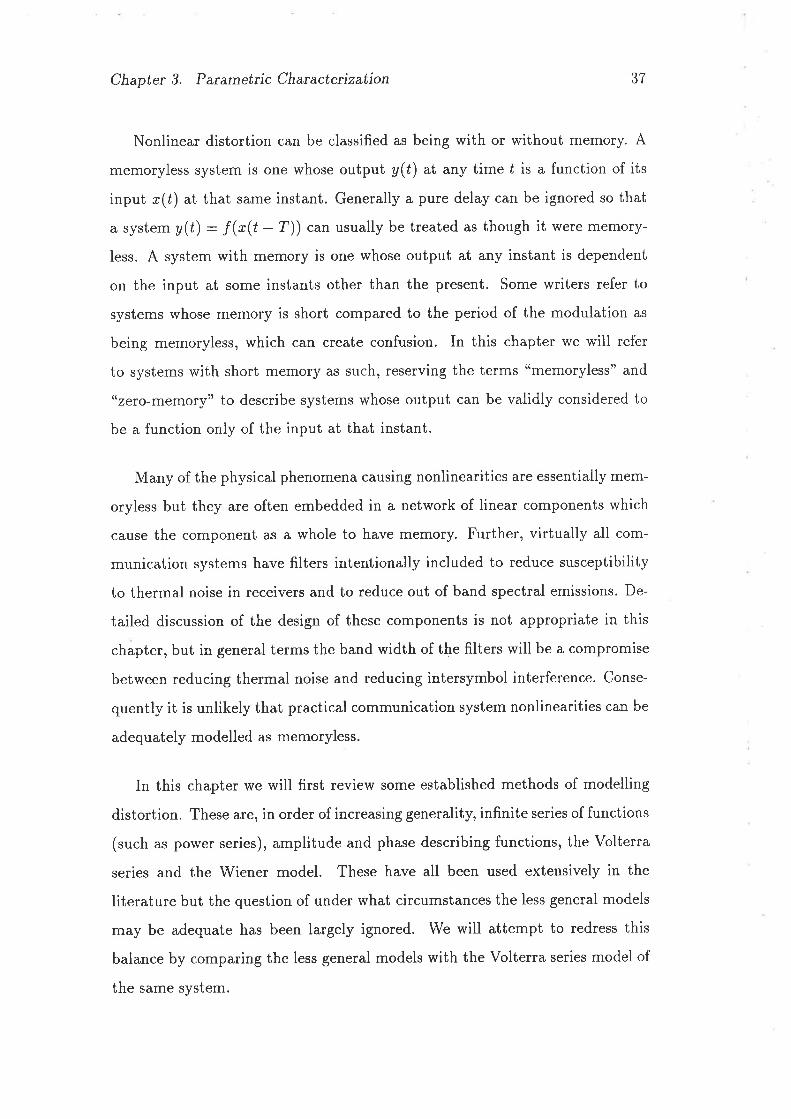
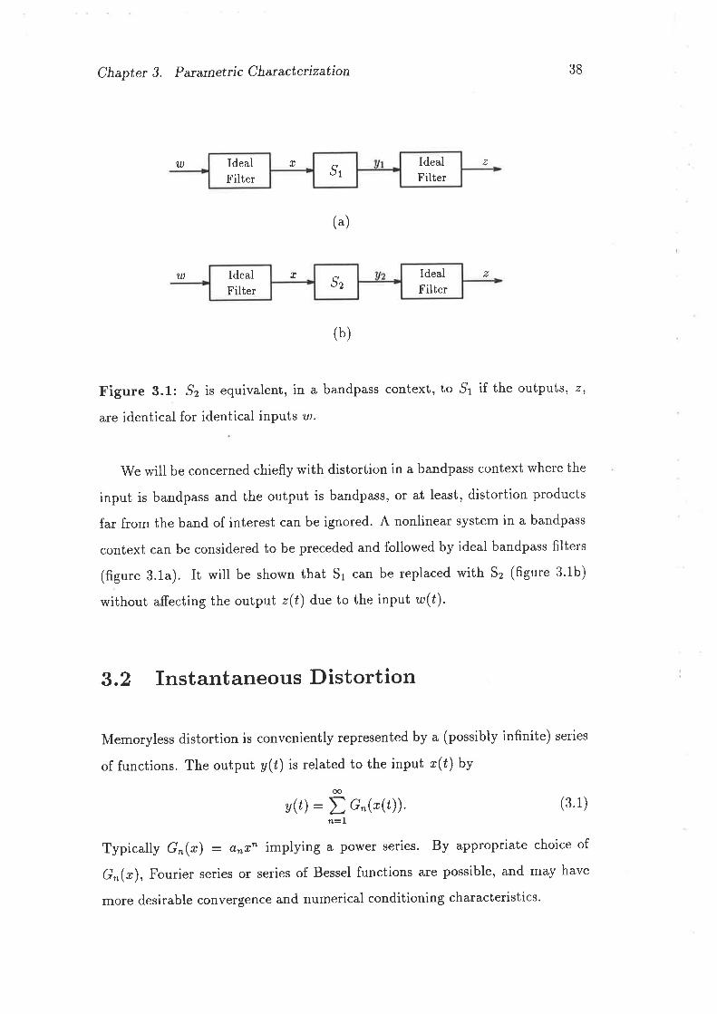
Chapter 3. Parametric Charucteñzation 38
(3.1)
w
u
T
T
þ
(u)
t
Figure 3.1: Sz is equivalent, in a bandpass context, to,9r if the outputs, z,
are identical for identical inputs u.'.
We will be concerned chiefly with distortion in a bandpass context where the
input is bandpass and the output is bandpass, or at least, distortion products
far from the band of interest can be ignored. A nonlinear system in a bandpass
context can be considered to be preceded and followed by ideal bandpass filters
(figure 3.1a). It will be shown that sr can be replaced with sz (figure 3.1b)
without affecting the output z(f) due to the input tr(l).
9.2 Instantaneous Distortion
Memoryless distortion is conveniently represented by a (possibly infinite) series
of functions. The output y(ú) is related to the input r(t) by
(b)
æ
n=laþ) : ! c"1"1t¡¡.
Typically G^(") : cr,n7n implying a power series. By appropriate choice of
G^(*),, Fourier series or series of Bessel functions are possible, and may have
more desirable convergence and numerical conditioning characteristics.
IdealFilter
IdealFilter Sz
Chapter 3. Parametric Chancterization 39
It is appropriate to note that a power series can be made to approximate
any function, and hence any memoryless distortion, arbitrarily well over a given
range (the Weierstrass theorem). Few communication systems are memoryless
or can be accurately modelled by a power series, yet the power series model has
been extensively used, and continues to be used because applying more accurate
models can present intractable problems. Sometimes it is possible to use the
zero memory model to work out worst case results. Because it is still used, and
also because it is the basis for later results we will now consider in some detail
the behaviour of a system modelled by a power series in a band limited context.
Assume the system is described by 3'1 with
G"(r(t)) - a,r"(t) (3.2)
and the input is
lrçt¡"i'*)(t 1t¡ "
i'ot * ã- (t) e- i'ot) (3.3)
The variable õ is the complex envelope of r defined by ã : (t + iû)ei'o', where
ô is the Hilbert transform of x. The asterisk superscript is used to indicate the
complex conjugate. Substituting 3.3 into equation 3.2 gives for one term of the
r(t) : ft1
2
power serles
G"(ø(t)) - ("0) * -' r') r. i çt7 etu - 2 i) i'lu s t'o"S'¡n L" i=O
(3.4)
If we now note that the ith term has the same magnitude centre frequency
as the /th term iln-2i: -(n-21) i.e. I:n- i. For n odd,
G*(*) : #'-Ë-'' l(:)*-,r-i"(n-2i)iuo'* (, "_ o)r,r.^-;e-@-z;)i-ot]
(3.5)
Chapter 3. Parametúc Charactetization
and for n even
nn-?,
40
(3.7 )
G,(*): #(n
n126nl2 i*n12
(nl2)-r+ti=O [
(î) t"-'t'ri "(n-2i)iuo'
+ ( -i ¡*n-i "-(n-2i)iust
(3.6)
If we now make use of the narrowband constraint and discard all terms
involving "!.njuot where n + I it can be seen by inspection of 3'5 and 3'6 that
the only term remaining has n odd and i : (n -l)12. Also makìng use of
(Ð : (,in) u"¿ ññ* : lil2 results in
G^(*) : ?"(, ! r,r)wr-' (ñ"i'o' * ñ*e-i'ot¡
o,n:-2@-t)
For n:l,3,5..
n lã|"-t,(n-I)12
Equation 3.7 shows that a zero-memory distortion can, when the inputs and
outputs are narrowband, be considered as a distortion of the complex envelope'
The output complex envelope f is given by
n= [å W(*[')t't'-l ' (3s)
since the multiplicative factor in 3.8 is a real function, then it has been shown
that there can be no phase shift in a system with zero memory distortion'
3.3 Amptitude and Phase Describing Func-
tions
The memoryless distortion represented by 3.8 can be generalized to include a
limited class of distortion with memory by allowing phase shift to be repre-
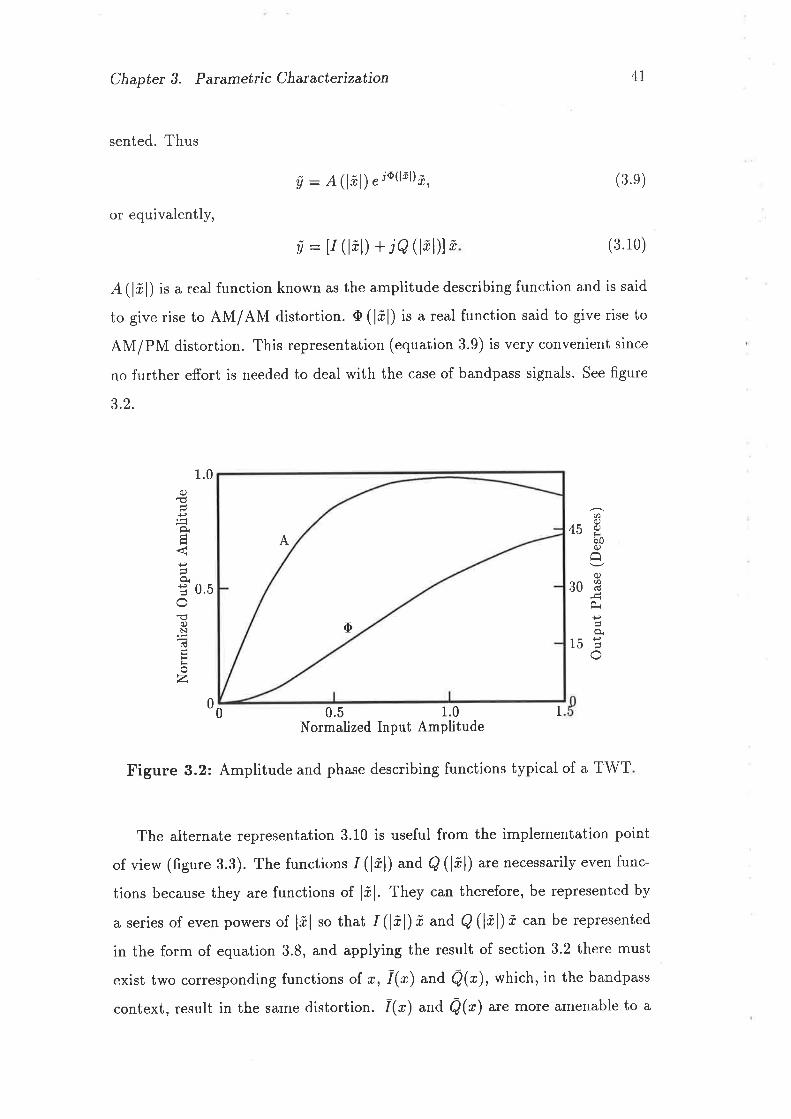
Chapter 3. Parametric Characterization +I
sented. Thus
ú : A(l¿l), iaG'Dã, (3.e)
or equivalently,
v : lr 0¿l) + je (rùlñ (3.10)
A(lñD is a real function known as the amplitude describing function and is said
to give rise to AM/AM distortion. O (lõl) is a real function said to give rise to
AM/PM distortion. This representation (equation 3.9) is very convenient since
no further effort is needed to deal with the case of bandpass signals. See figure
3.2.
.01
Ø
45Ëbo
Êc)
30reÈ
15E
0.5
c)
À4
È
q)N(!
iroz0
0 0.5 1.0Normalized Input Amplitude
1
Figure 3.2: Amplitude and phase describing functions typical of a TWT
The alternate representation 3.10 is useful from the implementation point
of view (figure 3.3). The functions 1(lõl) and Q (lãl) are necessarily even func-
tions because they are functions of lõ1. They can therefore, be represented by
a series of even powers of lil so that /(lf l)õ and A(lf)ã can be represented
in the form of equation 3.8, and applying the result of section 3.2 there must
exist two corresponding functions of r, I(ø) and Q@), which, in the bandpass
context, result in the same distortion. 1(z) and Q@) ate more amenable to a
A
Õ
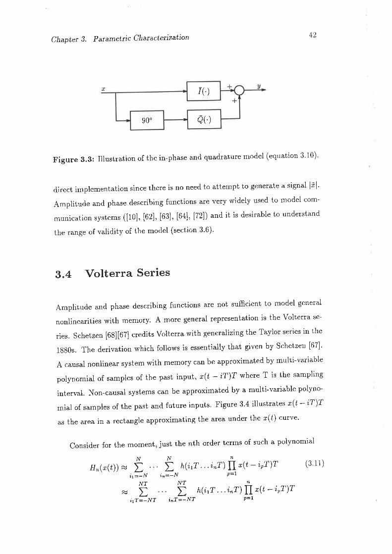
/(.)
0( )900
Chapter 3' Patametric Chancteúzation 42
r
Figure 3.3: Illustration of the in-phase and quadrature model (equation 3'10)'
direct implementation since there is no need to attempt to generate a signal lil'Amplitude and phase describing functions are very widely used to model com-
munication systems ([i0], [62], [63], [64], [72]) and it is desirable to understand
the range of validity of the model (section 3'6)'
9.4 Volterra Series
Amplitude and phase describing functions are not sufficient to model general
nonlinearities with memory. A more general representation is the volterra se-
ries. schetzen [68][67] credits voiterrawith generalizing the Taylor series in the
1g80s. The derivation which follows is essentially that given by schetzen [67]'
A causal nonlinear system with memory can be approximated by multi-variable
polynomial of samples of the past input, r(t - i?)? where T is the sampling
interval. Non-causal systems can be approximated by a multi-variable polyno-
mial of samples of the past and future inputs' Figure 3'4 illustrates r(ú - ff)T
as the area in a rectangle approximating the area under the r(ú) curve'
consider for the moment, just the nth order terms of such a polynomial
NNNH^(r(t)) x t t hU[ " 'i^r) II "(¿ - ipr)r (3'11)
;rJ.¡y i'=-N P=lNT N1tt h(i{ . ..i^r) fI '(¿ - ier)r
fL
i1T=-NT inT=-NT p=l
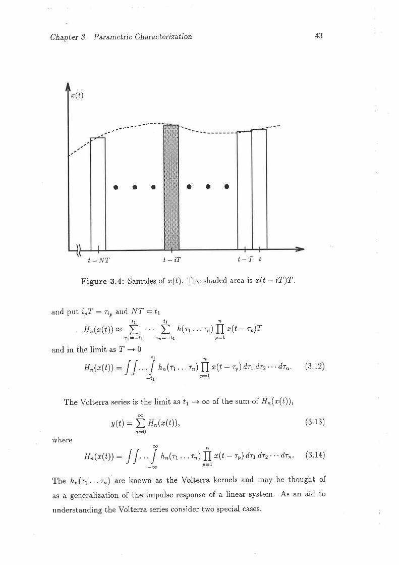
Chapter 3. Parametric Characterization
Ø(r)
43
(3.13)@
n=O
oo
-oo
oao oaa
t_NT t-iT t-T t
Figure 3.4: Samples of u (ú). The shaded area is ,(t - iT)T.
and put irT - r¡o and NT : ttt¡t1n
H^(r(t))x t t h(r'...'") lIx(t-rr)TT7=-tt f¡=-t! P=l
and in the limit ut t l
O 11 n
H^(x(t)) = I 1 .. I n*{rr...r^)lI.þ - r,)d,vd,rz"' d¡n' (3'12)
-t1 P=l
The Volterra series is the limit as f1 -+ oo of the sum of H"(t(t)),
y(t) : I n"1nçt¡¡,
where
H^(r(t)): ll ..I n*?, . t") fI r(t - rr) drl drz. . . drn. (3.14)n
p=l
The å,(1 ...rn) are known as the volterra kernels and may be thought of
as a generalization of the impulse response of a linear system. As an aid to
understanding the Volterra series consider two special cases.
Chapter 3. Parametúc Characterization
7. I1 h,(r1,r2...rn) : anfll=t6(rr), then y(l) : DÊo anx"(t),, which is a
power series (memoryless distortion)'
2. If h^Qy,r2...rn):0 for all n ) !, then the system is a linear one with
an impulse response of h1(21).
There is a theorem due to Fréchet which states that any functional can be
arbitrarily well approximated over a given range by a Volterra series. This
makes the Volterra series very general although systems with more than one
stable state (such as flip-flops) cannot be characterized by a Volterta series.
Determining the Volterra kernels hn(rr,rz. . .rn) of a system experimentally
is cumbersome and evaluating 3.13 in a simulation is expensive in computing
resources. The Volterra series does, however, provide a useful theoretical tool
and extensive use will be made of it in the rest of this chapter.
Note that the nth order term scales in proportion to A" where A is the
amplitude of the input signal. This can be verified by substituling Ar(t - rr)
for r(ú - rr) in equation 3.14. This property was previously (section 2.2) shown
for the case of zero memory distortion.
44
It can be shown ([8], Appendix A) that in the bandpass context, distortion
represented by 3.13 may equivalently be represented by
i t.,, - r;)e-i'o"i
2k+tx II ã(t - r;)¿raori dq dr2. ' .drn.
i=¡b41(3.1 5)
This is significant because it shows that, in a bandpass context, quite general
distortion of a signal can be modelled by distortion of the signal's complex
envelope. It is possible to go further and define a low pass equivalent of the
volterra kernel [8] but this is not required for the present purpose.
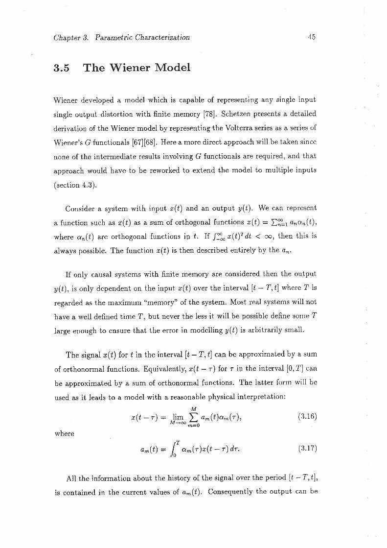
Chapter 3. Parametúc Characteúzation 45
3.5 The 'Wiener Model
Wiener developed a model which is capable of representing any single input
single output distortion with finite memory [78]. Schetzen presents a detailed
derivation of the Wiener model by representing the Volterra series as a series of
Wiener's G functionals [67][68]. Here a more direct approach will be taken since
none of the intermediate results involving G functionals are required, and that
approach would have to be reworked to extend the model to multiple inputs
(section 4.3).
Consider a system with input ø(ú) and an output y(ú). We can represent
a function such as r(ú) as a sum of orthogonal functions ø(f) : ÐÊr a.an(t),
where a,(t) arc orthogonal functions in ú. If /å x(t)2 dt ( oo, then this is
always possible. The function r(t) is then described entirely by the ø,,.
If only causal systems with finite memory are considered then the output
y(l), is only dependent on the input r(ú) over the interval [¿ - 7,ú] where T is
regarded as the maximum "memory" of the system. Most real systems will not
have a well defined time 7, but never the less it will be possible define some ?
large enough to ensure that the error in modelling y(t) is arbitrarily small.
The signal r(ú) for f in the interval lt-T,t] can be approximated by a sum
of orthonormal functions. Equivalently, r(t - r) for r in the interval [0,?] can
be approximated by a sum of orthonormal functions. The latter form will be
used as it leads to a model with a reasonable physical interpretation:M
*(t - ') : Ji31 I ø-(t)o*(r), (3.16)m=u
whererT
a*(t) : I a,"(r)x(t - r) dr. (3.17)Jo
All the information about the history of the signal over the period [t - T,t],
is contained in the current values of a^(t). Consequently the output can be
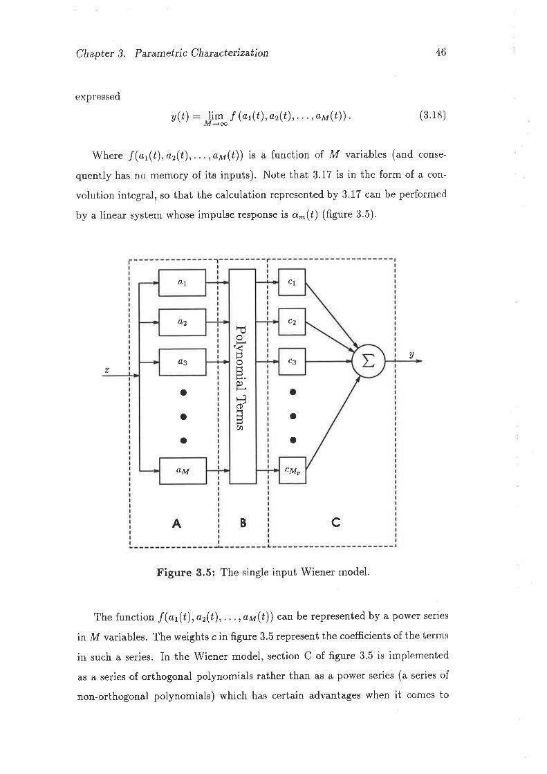
Chapter 3. Parametric Characteúzation 46
expressed
y(t) : Jlg / (o'(¿), or(t),. . ., "r(t)) . (3.18)
lVhere f@t(t),or(t),...,ov(t)) is a function of M varial:les (and conse-
quently has no memory of its inputs). Note that 3.17 is in the form of a con-
volution integral, so that the calculation represented by 3.17 can be performed
by a linear system whose impulse response is a-(ú) (figure 3.5).
tl
vr
B
Figure 3.5: The single input Wiener model.
The function /(ø1(t),,ar(t),...,"*(t)) can be represented by a power series
in M vaiables. The weights c in figure 3.5 represent the coefficients of the terms
in such a series. In the Wiener model, section C of figure 3.5 is implemented
as a series of orthogonal polynomials rather than as a power series (a series of
non-orthogonal polynomials) which has certain advantages when it comes to
A c
C1A1
C2A2
C3ûs
o
o
a
o
O
o
cMpaM
FÚo)Hr-{
p
Ë(DH
U)
Chaptet 3. Paramettic Characterizatton 47
devisingarapidlyconvergentstrategyforadjustingtheweightsc.
It can be shown (Appendix B equation 8.4) that a function of several vari-
ables may be rePresented asM
t rrl2 ¡... ¡rn M II I * rP nçt¡¡'q=l
(3.1e)
oo cott oo
/(or(¿), az(t),. . . ,o,M(t)) - m1=Om2=O 'mM=O
TheB^o(ao(Ú))inequation3.lgaresingledimensionalorthonormalfunctions
such that 0, il. i@;(a*(t))Þi(¿-(¿))) :
1 if(3.20)
Jf Jj
Since the o-(ú) are functionals of r(ú) defined by equation 3'17 we can
express equation 3.19 as
/(or(¿), az(t),.. ' ,ono(t)) :co oo oo
and
t tt b^ r,^r,...,*, ó ^r,^r,...,^ * (* (¿))
m1=Om2=O m¡4=O(3.21)
From equation 3.19 and equation 3'21
ó mt,rnz,...,m- (t (¿ ) ) : 0 ^t@'(t)) þ ^,(o'(t))''' þ ^ * (o *' (t))'
ó k,,k,,...,k u(r (¿) ) = þ x,(o, (¿) ) É¡, ( or(t))' " þ t', (o u (t))'
ConsequentlY the Ó^r,^r,...,^*
tionals with the ProPertY that1 if. m¿ - kr for i : 1,2, "' , Mi
otherwise.(ó ^r,^r,...,^, (" (t)) Ó ur,rr,"',tt ( r (t) ) ) - 0,
(3.22)
The notation in equation 3.22 can become a little cumbersome' so we define
iri*i;\f.i-¡.
("(¿)) can be considered orthonormal func-
01
the Kronecker delta function
6;t:
Chapter 3. Panmetúc Characteúzation 48
We can then rewrite equation 3.22 as
M(Ó^ r,*r,...,^ * (* (t)) Ó rr,xr,...,* * (x (t) ) ) : fI ó-rt,
q=L(3.23)
Multiplying both sides of equation 3.21 by ökr,kr,...,kr(t(ú)), taking the aver-
age, exchanging the order of the summation and the averaging, and eliminating
terms which are zelo by property equation 3.23, we obtain
bk,,k",...,k * : (f (a1(t), az(t), . . ., " u (t)) Ó n,,x,,...,*, (t (¿) ), )
and by simply changing the variables,
b^r,^r,...,^, : (/(a1(/),az(t),...,ou(t))ó^r,^",,..,*.r(r(¿))) (3.24)
Equation 3.24 implies that the b^r,^r,...,m¡,¡ câ;lbe determined by a simple
correlation.
Up to this point the development has been independent of the choice of the
sets of orthogonal functions. The choice of the p^r@o(t¡¡ is complicated by the
fact that ao(ú) is typically a random variable whose distribution must be taken
into account. The p^r@n(t¡¡ must satisfy equation 3.20 which can be rewritten
AS
l* g,{o)g,þ)p(o) d' : {o, ifilj1, ili:i; (3.25)
where p(a) is the probability density function of ø and can be thought of as the
fraction of the time which ø spends at a particular amplitude. More precisely,
p(as)da is the fraction of the time for which as 1 a 1 ao * da.
The choice of the g^,þo(t¡¡ is governed by the probability density function
of its inputs. Wiener and others have assumed that the øo are Gaussian dis-
tributed with a probability density function of. p(a) - "-a2/zo2 ¡(oQi). If the
0^þ) are considered to be polynomials of the form B*(a) : DiLo c¡an then
the coefficients c¡ can be determined uniquely by applying equation 3'25. The
rnth degree polynomial must be orthogonal to all lower order polynomials. If
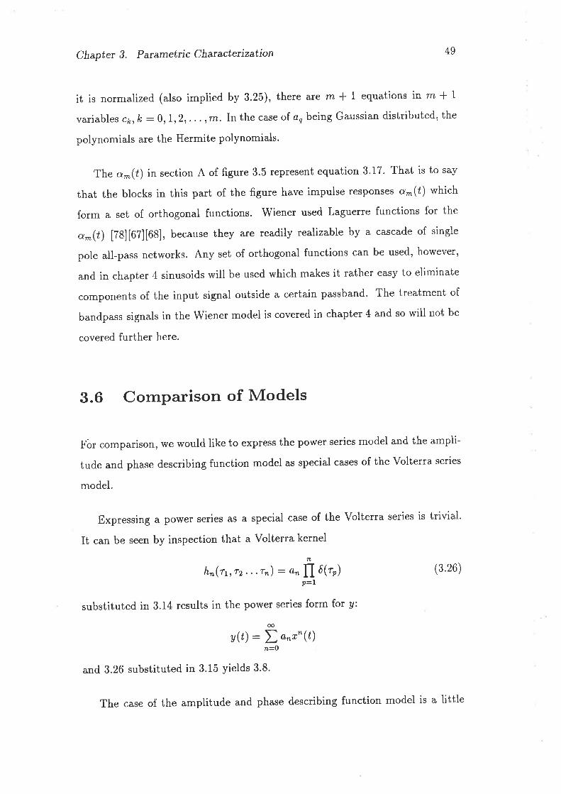
Chapter 3. Parumetric Characterization 49
it is normalized (also implied by 3.25), there are rn { 1 equations in m * |
variables c¡,le :0,1,2,. .. ,,T'n. In the case of øo being Gaussian distributed, the
polynomials are the Hermite polynomials.
The a-(t) in section A of figure 3.5 represent equation 3.17. That is to say
that the blocks in this part of the figure have impulse responses a-(ú) which
form a set of orthogonal functions. Wiener used Laguerre functions for the
a^(t) [78][67][68], because they are readily realizable by a cascade of single
pole all-pass networks. Any set of orthogonal functions can be used, however,
and in chapter 4 sinusoids will be used which makes it rather easy to eliminate
components of the input signal outside a certain passband. The treatment of
bandpass signals in the Wiener model is covered in chapter 4 and so will not be
covered further here.
3.6 Comparison of Models
Fôr comparison, we would like to express the power series model and the ampli-
tude and phase describing function model as special cases of the Volterra series
model.
Expressing a power series as a special case of the Volterra series is trivial.
It can be seen by inspection that a Volterra kernel
n
lrn(rr,rz . . .rn): ø" f[ ó(ro)P=7
substituted in 3.14 results in the power series form for y:
(3.26)
y(t) : I a*u"(t)oo
n=O
and 3.26 substituted in 3.15 yields 3.8.
The case of the amplitude and phase describing function model is a little
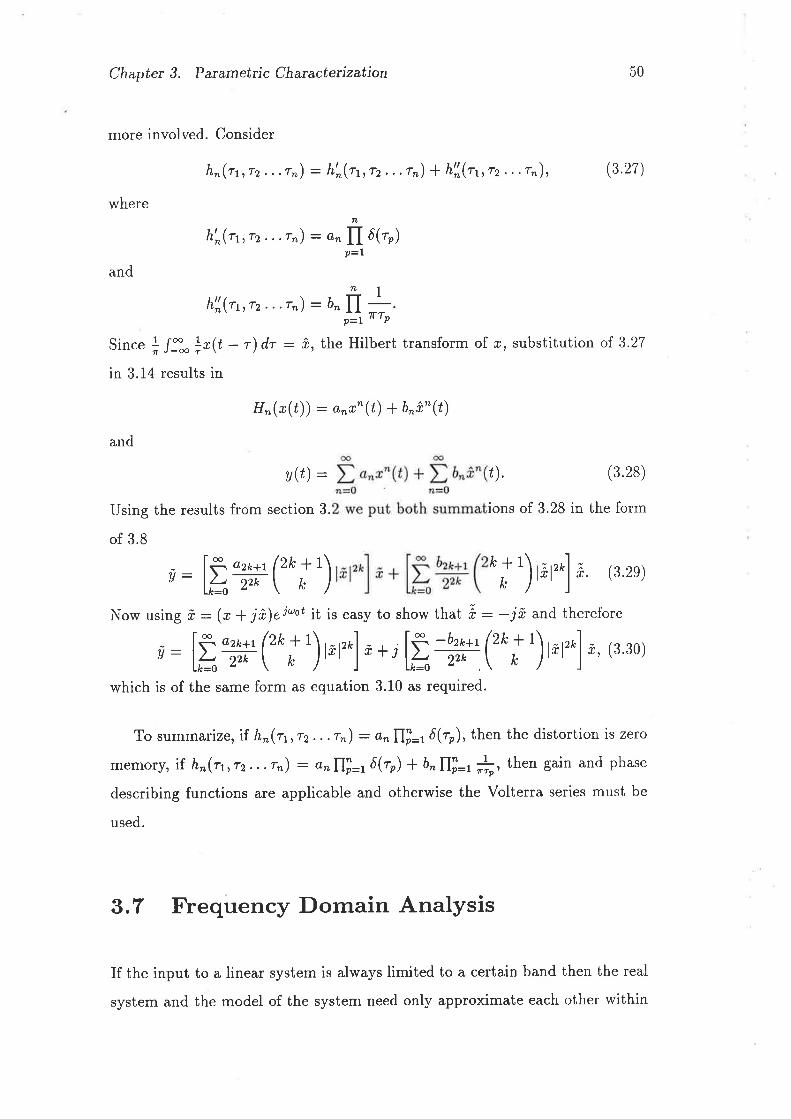
Chapter 3. Parametric Characteúzation 50
more involved. Consider
hn(rt,rz. . .r,-) : h'^(r1,T2... rn) I h'l(r1,r2.. .rn), Q.27)
where
h'n(rt,,rz . . . Tn) : o^fi 6¡r¡p=l
and
L,t12...rn) : U"lI +.p=l TTn
Since * l: l*(t - r) dr : â, the Hilbert transform of r, substitution of. 3.27
in 3.14 results in
H"(r(t)) - a,x" (t) + b"î" (t)
Now using ñ : (r + jã')ei'ot it is easy to show that â : -ii and therefore
and
y(t): t). (3.28)
Using the results from section 3. ions of 3.28 in the form
of 3.8
ú-lÐ--æ('***') ***') ãrr]' (32e)
û : läæ( [') r'r'-] ã + ilä+(r i') r'r'-]
which is of the same form as equation 3.10 as required.
r, (3.30)
To summaÅze,if. h,(rr,rz...rn) : anfll=t6(rr), then the distortion is zero
memory, if. h^(r1¡r2...rn) : anl\=t6(rr) * b,Í|i=t fr, th"tt gain and phase
describing functions are applicable and otherwise the Volterra series must be
used.
3.7 Flequency Domain Analysis
If the input to a linear system is always limited to a certain band then the real
system and the model of the system need only approximate each other within
Chapter 3. Parametric Characterizatton
ün(t¡tr, ,tn): I I I
51
uu)
HX
)
)
Q1 Q2u
Figure 3.6: Frequency lange of interest for a linear system' If the input,
lx(r)1, is band limited toal--uy then the system lesponse outside that range
need not be considered.
that band (see figure 3.6). It would be useful to be able to relax in a similar way
the approximation of a real nonlinear system by a model. Just as for the linear
case, it is most convenient to handle this problem in the frequency domain'
Define
y^(t) = H"(x(t)),,
also defineft
d,r1 d,r2 . . . drn hn(r, .. . "") fI x(to - rr) 'P=1
(3.31)
By reference to 3.14 it is apparent that
y^(t) : ùn(t,t,. . ., ¿).
Taking the n-dimensional Fourier transform of 3.32 results in
(3.32)
Y,"(rr, u2¡ . . .u,") : Hr,(r, ¡Q2¡ . .. r") ll X('o)'fL
p=7(3.33)
Chaptet 3. Parametric Characterizatton
É_
V.
52
t!2
tÐ3
t!1
l----.71
ií i
')- - - -.J
,r
t-,:ai
iiIIII
t¿-
I
fIILII
,ij-__i.
.lí,- -,,.
I
t¿-
II
v-__-J
I
t-II,E-
IIII
,fIIIII
III
III ----J
I
1I
Figure 3.7: A cube of interest in 3 dimensional frequency space.
It is apparent from 3.32 that Y,(r) is dependent on Y"(ø r,te2¡ . . . ,an) although
we don't need to find the exact ¡elationship for our present purpose. If we now
assume that r is bandpass, i.e.
Xo(tr) :0, forløol (øo-e,orlørl )eole, (3.34)
then the output is independent of H,n(rr ¡u2¡...ø,") except for cu within the
hyper-cube defined by ,o - e ( lrol < uo * e (see figure 3.7).
Let us now apply the limited frequency space of interest to the case of the
Chapter 3. Parumetúc Charucterization 53
po\¡/er series in amplitude and phase describing function models. We need to
find H"(c,.rr¡a2t...ø.n) for these two cases. Taking the n-dimensional Fourier
transform of 3.26 and 3.27 results in
Hr,(rt ¡u2r, ..un) : an, ( 3.35)
for the case of a pov/er series and
iH'(rr,,(Ð2,t. . .rn) : an * bnfl -¡sgn(øo),p=7
for the case of amplitude and phase describing functions.
(3.36)
The n-dimensional Fourier transform lJn(rt,. . ,r^) of any realh,.(n,. . . ,rn)will have its real part symmetric with respect to øo and its imaginary part anti-
symmetric with respect to uo. This property is well known for single dimensional
Fourier transforms, and its extension to n-dimensional Fourier transforms fol-
lows by considering an n-dimensional transform as n single dimensional Fourier
transforms. It follows therefore that any system representable by a Volterra
series can be approximated arbitrarily well by amplitude and phase describing
functions over a narrow enough band width as long as the limit as e -- 0 of
H,(ro * €,...,@o * e) exists.
As a direct consequence, testing a system with a sinusoid (a signal of zero
band width) is insufficient to determine whether a system can adequately be
modelled by amplitude and phase describing functions (unless, of course, the
model will only be used with a sinusoidal input). Both 3.35 and 3.36 are inde-
pendent of ø; and it might be thought that testing with a sinusoid at a number
of different ø6 would be sufficient to check whether amplitude and phase de-
scribing functions are an adequate description. This is not the case however.
The response of a system to a sinusoid of every frequency within the band of
interest depends on Hr,(u.r1 , ...run) along a line, Lùr : (Ð2 : ... : u)n : u)o,t
through the hyper-cubes of interest in the n-dimensional frequency space. As
an example consider the third order system defined by
Ht(rt) : a7¡
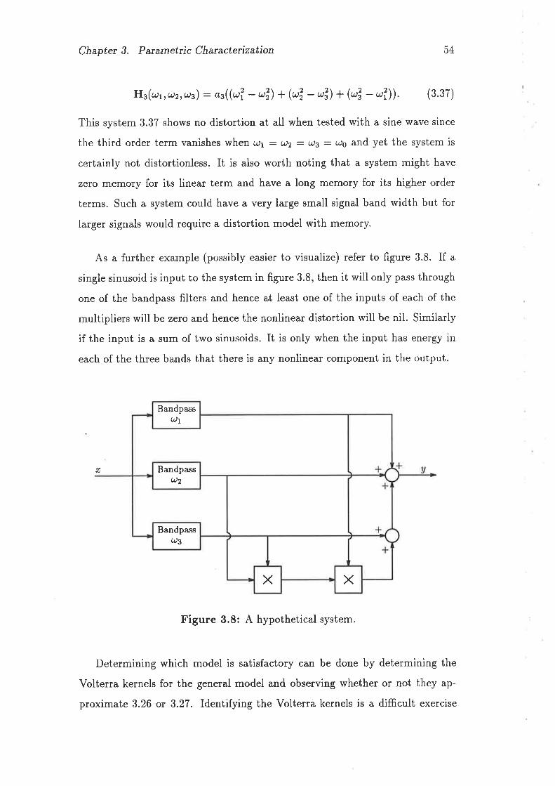
Chaptet 3. Parametric Chancterization
Hr(rr, uz,,,s) : as((al - rÐ + @3 - rÐ + @3 - rï). (3.37)
This system 3.37 shows no distortion at all when tested with a sine wave since
the third order term vanishes when o)r : u)2 - u)B : ûJs and yet the system is
certainly not distortionless. It is also worth noting that a system might have
zero memory for its linear term and have a long memory for its higher order
terms. Such a system could have a very large small signal band width but for
larger signals would require a distortion model with memory.
As a further example (possibly easier to visualize) refer to figure 3.8. If a
single sinusoid is input to the system in figure 3.8, then it will only pass through
one of the bandpass filters and hence at least one of the inputs of each of the
multipliers will be zero and hence the nonlinear distortion will be nil. Similarly
if the input is a sum of two sinusoids. It is only when the input has energy in
each of the three bands that there is any nonlinear component in the output.
54
fr
Figure 3.8: A hypothetical system.
Determining which model is satisfactory can be done by determining the
Volterra kernels for the general model and observing whether or not they ap-
proximate 3.26 or 3.27. Identifying the Volterra kernels is a difficult exercise
BandpassU1
Bandpassu2
BandpassQ3
X X
Chapter 3. Parametric Characterization ,5t)
which has received some attention in the literature [4] [68]. Here we shall do
no more than consider the minimum complexity signal which could be used
to identify the Volterra kernels. Since there are n independent variables in
Hr(rt ,. . . ,an) it is reasonable to consider an input of n sinusoids whose trans-
form has the form
X(r) : D la,6(u - -tr) * ai6(w+ 7r)1. (3.38)TL
p=L
When substituted in 3.34, Y"(rr, ti2,t . .. ø,,) consists of a sum of (2r)" terms,
some of which are like
dta2. . 'anHn(.yt) /2,. . ..ln) (3.3e)
Actually isolating terms like 3.39 from all the rest of the terms requires a
testing strategy which is cumbersome to devise and impractical to implement
(see [a] for some special cases). However, the existence of terms like 3.39 show
that n sinusoids of frequency ^lp can be used to identify an nth order system
at most. It is important to note that the vector ('yr,1r,. . . ,l^) must be set
to every point in the hypercube of interest within the n-dimensional frequency
space defined by ,o - e 1 1p 1 uo * e in order to competely characterize
Hr,(rt, u2). . ,ø,,.).
3.8 Summary
The distortion in systems modelled by power series, amplitude and phase de-
scribing functions and Volterra series has been analyzed for the case of bandpass
inputs and outputs. In all cases it has been shown that distortion in a bandpass
context can be considered as distortion of the complex envelope of the signal.
This is of significance from the point of view of distortion correction in commu-
nication systems, since it means that distortion can be corrected at baseband
o¡ at some intermediate frequency as effectively as it can be at RF.
Chapter 3, Parametric Characteúzation bb
The power series model was shown to be a special case of the amplitude
and phase describing function model. Both the po\ryer series model and the
amplitude and phase describing function model were shown to be special cases
of the Volterra series model and the form of the Volterra kernels was deduced.
The Wiener model of nonlinearities has been derived.
From consideration of the frequency domain representation of the Volterra
kernels it was shown that, for band limited inputs, the Volterra kernels of the
model and of the actual system need only match for ø within a hyper-cube of
interest. This is analogous to requiring the model of a linear system to match
the actual transfer function over a frequency range of interest.
It was also possible to show that for a sufficiently narrowband input signal,
any distorting system describable by a Volterra series could be approximated
by the amplitude and phase describing function model. It was also shown that
testing with a single sinusoid, even at a number of different frequencies, is
inadequate to check whether amplitude and phase describing functions are an
adequate model or whether a more general Volterra series model is necessary.
Frequency independence of the amplitude and phase describing functions, as
measured by a single sinusoid is a necessary, but not sufficient condition for the
amplitude and phase describing function model to be applicable.
Chapter 4
Multi-input Systems
4.L Introduction
The work in this chapter was mostly covered in an earlier paper by myself
[23]. Radio communication systems make extensive use of mixers to perform
frequency translation. A discussion of the architecture of receivers is beyond
the scope of this chapter but high performance receivers typically have two or
three separate frequency conversion operations.
The distortion of a signal going through a time invariant single input single
output system can be modelled as a distortion of the complex envelope of the
signal [8][24]. If the frequency translation operations are ideal (but the rest of
the system is not) then the complex envelope of the signal is unchanged by the
frequency translation process and distortion of a signal going through the whole
system can be modelled as a distortion of the complex envelope of the signal.
Unfortunately real mixers are not perfect and contribute to the distortion
of the signal. Further, in many modern communication systems the mixer
does not perform a simple frequency conversion. In radar systems the local
Ðt
Chapter 4. Multi-input Systems 58
oscillator might be a "chirp" (linear frequency sweep) signal, and in frequency
hopping spread spectrum systems the local oscillator might follow a series of
step functions in frequency. These two factors prevent the treatment of the
distortion caused by a receiver as a single input, single output, time-invariant
distortion of the complex envelope of the signal.
A typical communication system is, in reality, a multiple input device where
the inputs consist of the signal being processed and all the local oscillator signals.
It is of interest therefore to determine a model of minimum complexity, which
is still sufficiently general to represent such systems adequately.
In section 4.2 of this chapter a simple model of distortion in mixers will be
presented and it will be shown to be capable of representing the distortion in a
mixer under restricted conditions.
The Wiener model of a nonlinear system presented in chapter 3.5 will then
be extended to systems with more than one input. The extended Wiener model
(which is quite general) will then be compared with the simple model presented
in section 4.2 and the conditions under which the simple model is adequate will
thereby be established.
In many systems the phases of the local oscillators relative to the input
signal and to each other are not controlled. In these cases the absolute phase
of the output is not important. If the phase of the local oscillator changes
by a constant amount, the phase of the desired output signal changes by a
constant amount. It will be shown that under appropriate bandpass conditions
the distortion components also change phase by a constant amount. This is
important because otherwise the spectrum (and maybe even the total power) of
the distortion would depend on the phase relationship between the input signal
and the local oscillator and it would impossible to devise a deterministic model'
Mixers are almost always used in a bandpass context. That is to say that a
Chapter 4. Multi-inPut SYstems 59
mixer,s ìnputs are bandpass and that its output is bandpass fiitered (or at least
that frequency components outside a certain band of interest can be ignored)'
In this chapter only the bandpass case will be considered'
Thetwoinputbandpasscontextisdefinedthesamewayassingleinput
bandpass context (see section 1.1.2) except there is an ideal filter in each in-
put.Inthecaseoftwo-inputbandpasssystems,theoutputwilldependonthe
frequencies of the inputs and of the filters centre frequencies' The output filter
is normally arranged to be centred on either the sum or the difference of the
two input frequencies. It is possible that harmonics of an input signal will also
be within the output passband. We assume in this chapter' that the system ts
designed so that this does not occur'
4.2 A Simplified Model Of Two Input Non-
linearities
The distortion specifications quoted by most mixer manufactulers ale the two
tone intermodulation intercept points and the compression point' Since a dis-
tortion with memory can not be adequately tested by one or two tone measure-
ments [24], manufacturers and designers are implicitly assuming that mixers are
zero memorY devices'
Further, since the local oscillator signal does not appeal as a palameter in
the distortion specification (except to specify how large a signal it should be)'
the mixer is implicitly being treated as a single input device' certainly the
specifications based on these assumptions are convenient from the point of view
of the designer, but the question of how valid the assumptions ale' remains'
Figure 4.1 illustrates such a system. The multiplier represents an ideal mixer
and .|ú, and' N,, represent single input, single output distortions. First assume
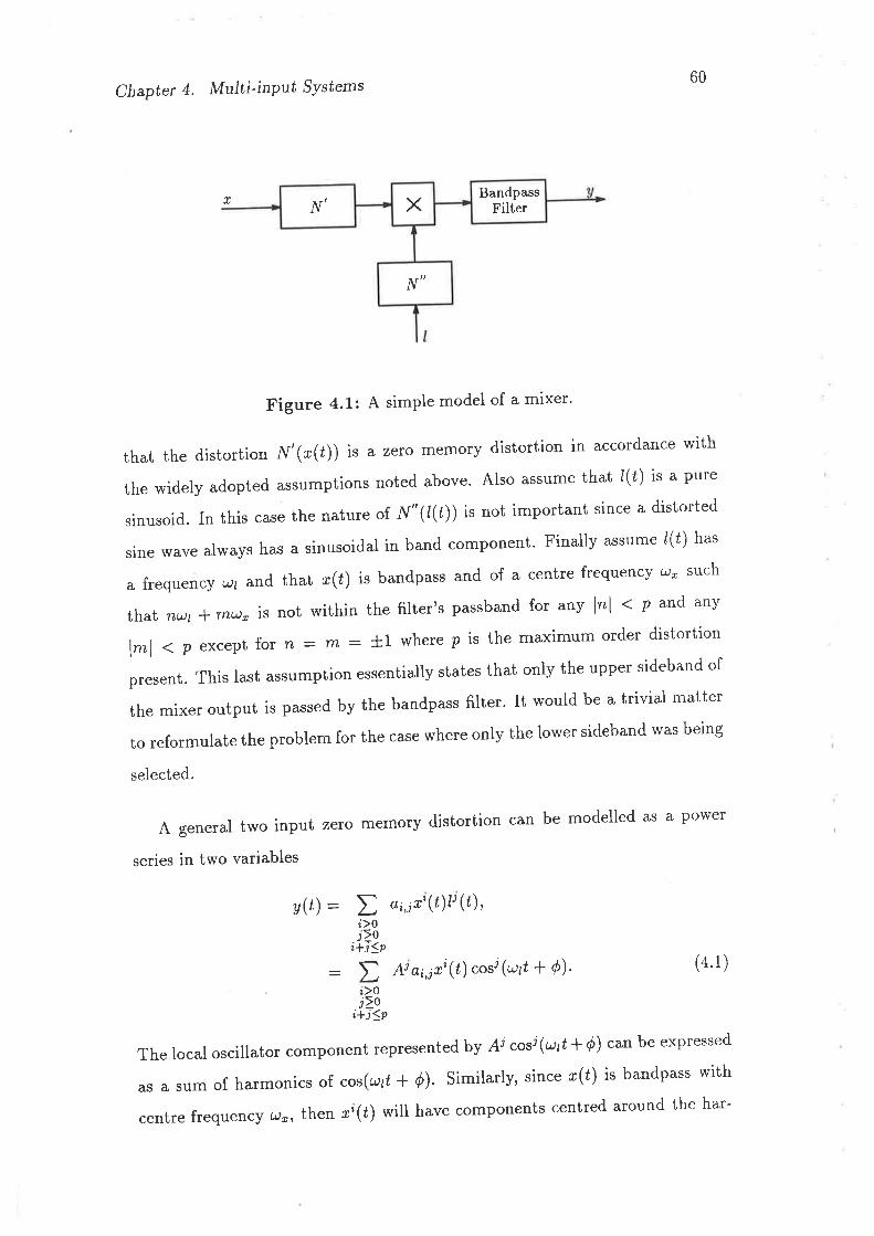
BandpassFilterXN,
t,N
60Chaptet 4. Multi-inPut SYsúems
r
Figure 4.1: A simple model of a mixer'
that the d,istortion N'(z(t)) is a zero memory distortion in accordance with
the widely adopted assumptions noted above' Also assume that /(ú) is a pure
sinusoid. In this case the nature of N"(l(ú)) is not important since a distorted
sinewavealwayshasasinusoidalinbandcomponent.Finallyassume/(ú)has
a frequenc} tl¡ and that r(Ú) is bandpass and of a centre frequency t,¡,,' such
thatnul*mu"isnotwithinthefilter'spassbandforany|"1<pandanyl-l<pexceptforr¿-_TT¿:tlwherepisthemaximumorderdistortionpresent. This last assumption essentiaily states that oniy the upper sideband of
the mixer output is passed by the bandpass filter' It would be a trivial matter
to reformulate the problem for the case where only the lower sideband was being
selected.
A general two input zero memory distortion can be modelled as a powel
series in two variables
a(t) -- t ai,ir'(t)lr (t),i>0j>0
i*i<p: t Ara;,¡xi(t)"ori(r¡f + Ó). (4 1)
i>0,l>¡2,
The local oscillator component represented by ¡i çssi (u¡tf /) can be expressed
as a sum of harmonics of cos(ø¡f + d). Similarly, since r(t) is bandpass with
centre frequency ø,, then ci(t) will have components centred around the har-
Chapter 4. Multi-inPut SYstems 61
monics of u,the form
The oniy terms which have energy within the passband are of
y(t) : t Ai a;,¡x'(t) cos(ø¡l * d)i>oj>0
i+ jíp: cos(crr¡ú + d) t a;r'(t),
i>0i3P
where t a;,j (4 3)i>0¡lî3p
Eqtration 4.2 is in the form of a product of the local oscillator signal and the
distorted signal. The same result is derived rather more rigorously in appendix
c using a complex envelope representation of r(ú). Also observe that in 4'2 the
locai oscillator signal has not been distorted and so N"(¿(ú)) : /(¿). It has been
shown, therefore, that a two input device with zero memory and a pure sinusoid
applied to one input can, in a bandpass context, be modelled as a combination
of a single input distortion and an ideal mixer (muttiplier)' Note, however, that
the distortion is dependent on the amplitude of the local oscillator'
A nonlinearity with memory implies that the output at any instant is depen-
dent on the inputs at all preceding instants within the memory of the system'
such a system is rather more difficult to describe in a generai way'
4.3 The 'wiener Model of Multi-input Non-
linearities
Before the wiener model can be applied to two input devices such as mixers,
it must be extended. A similar argument will be used for the two input case as
was used, for the one input case (chapter 3.5). For the pulposes of this chapter,
there is no advantage in representing ,f of equation 3'18 as a series of orthogonal
functions so the simpler power series representation will used.
(4.2)
Ao,i I
Chapter 4. Multi-inPut SYstems 62
The two inputs r(t) and l(ú) can both be represented by a series of orthonor-
mal functions
r(t - r,): J,gL I o-(t)o ^(r"),fn= L
(4 5)
(4.4)
(4.6)
(4.7)
where
where
1,,o^(t) -- a^(r)r(t - r,) dr,,
andN
b^þ): Io B^Q¡)x(t - r¡) d'r¡T
All the information about the two inputs over the interval lt - T,f] is con-
tained in the current values or a^(t) and ó'(t) so that the output of the system
can be expressed
a þ) : I @r(t), oz(t),' ", a u (t), br(t), b2(t)''''' b¡r (t) )'
The function, /, is of the same form as for the single input case (but with
more variables) and the same comments regarding implementation apply' The
operation performed by the function / is represented by the blocks in sections
B and C of figure 4.2
4.3,L TheTwolnput.WienerModelAppliedtoMixers
It is convenient to choose the impulse responses a-(Ú) aIId B^þ) to be sinusoids
over the interval [0, T]. These impulse responses will be harmonics of' s\n(2rt lT)
and cos(2zr tlT). The blocks in section A of figure 4.2 become, therefore' narrow-
band filters whose band width tends towards zero as ? tends towards infinity'
since the signals r(t) and /(t) are assumed to be bandpass, then any of the
filters o and B which have a passband outside the band of the signals need not
Chapter 4. Multi-inPut SYstems 63
be included in the model. The impulse responses of the filters which are within
the passband can be described
-. l(,,*o,ç) '] ,
for rn odd and 0 <t <T;
".. i(," ¡ n @))t+"nf ,
L\ for rn even and 0 < t ]=T;
0, otherwise;
.".[(,,*o"ç) 'l ,
(4 8)o^(t) --
and
for zz odd and 0 <t <T;
-,f(,, ¡t 9))t+"n), (4.e)0^(t¡ : ,
0,
for n even and 0 <t <T;
otherwise,
where
Lu :2r lT
The outputs of the filters o^(t) and b,¿(ú) are narrowband and tend towards
being sinusoidal as ? tends towards infinity (the ø,(t) and the ó-(t) then become
a representation of one sided Fourier transform of the signal)' In a practical
implementation it would be undesirable to let ? be larger than necessary be-
cause of the associated increase in the complexity of the model' To develop the
theoretical results in the rest of the chapter, however, the limiting case ? -+ oo
will be used and the outputs of the frlters in section A of figure 4'2 can be
written
o,^(t) - cos((-),
for rn odd;
for m even;
where
. I (,"+¡,@/) t*o*,t* =
I (r" + L,ry)t + r12* o^,
64Chapter 4. Multi-inPut SYstems
r
O,l
a2
el
€2
a
o
a
aM eB
b1
bz
o
o
O
eMpo
o
a
FÚo
oH
Êt¡
ÊoHU)
b¡a
u
A B c
Figure 4.22 The two input Wiener model
and
Chaptet 4. Multi-inPut SYstems 0b
(4.10)
b,(t) : cos(r¡-),
wherefor n odd;
for n even
(4.11)
It is now only necessary to write down a representation for the func-
tion / (or(¿), or(t), " .,av(t),h(¿), ó2(¿), ' ' ', óno(¿)) to complete the model' We
choose a multi dimensional power series,
pp
f (,,+r,þ*) t*ön,
'": l(,,* ml'59. )t*rl2*ón,
f (or,or,''''¡aM',
brrbzr...,óru)å¡ =0kz=o
iu=o fr¡v=O
(" j r,jr,...,j *,,hr,fr2,...,,b¡v
x a\'ai "'ar¡ff
x tf'uf'. . .åîf )
tlimp+Oo t
it=oiz=o
(4.12)
The e¡r,¡r,...,iM,lrt,kz,...,lrv, in equation 4'L2 are constant coefrcients' Since the
j- and k,, range from 0 to p then evely possible term of order less than or equal
to p is present. However, equation 4.12 also contains terms of order greater
than p. For example when every variable is raised to the maximum power p
then the term is of order (N + M)e ' There is no loss of generality in including
these terms since the associated coefficients can always be set to zero if a finite
order system is to be rePresented'
This model will now be used to show that a two input nonlinearity with
memory can not,'in general, be put in the form of figure 4'1'
Substituting 4.10 in 4,I2 and setting all the bn:0, the single input system
Chapter 4. MultïinPut SYstems
.nú'(ø(t)) can be written
N' (r(t)) : Ë (",,,,,,...,,,cosi'((1) cosi'((2) ' ' ' cosrM ((t)) ,
66
(4.13)jr =0J2=o
iu=o
and substituting 4'11 in 4'12 and setting all the dm:0¡ the single input system
¡f"(¿(¿)) can be written
N" (/(t)) : Ë (dr,,0,,...,**cosfr'(41)cosÀ'(42) "'"osÉ'(nt))' (4'14)/c1=0k2=O
È¡=0
The output of a system of the form in figure 4.1 can be written as the
product of equations 4.13 and 4.14
pp1ú'(r(t))¡ú" (/(¿)): t t
ju=O Ë¡v=0
and a general two input nonlinearity can be written
N (r(f), ¿(¿)) :pt=0=0
pt
(" jr,jr,...,j, d k1,k2,...,tc ¡¡
x "ori'((r) "orir((r) . . .cosr, ((¡ø)
x .orÈ'(Tr)"orfr, Ør). .. .o.ßt(ry")).
(4.15)
it--oiz=o
k1=Ok2=O
J1J2
,b1=Olc2=O
Ê¡y=O
(" j r,j",...,j *,È1,fr2,...,fr ¡y
x cosil ((1) cosi'((2)
x coskl(41)cosfr'(72)
cosrM ((¡a)
, cosßrv (ry"))iu=o
(4.16)
Clearly 4.15 is of the form of 4.16 if, and only if
€ jt,jz,.,.,j v,kr,È2,...,frN : ch,iz,..,,i u dkr,kr,.,.,k w,
for 0 ( j^Spand 0 1 kn1 P' (4.17)
Chapter 4. Multi-inPut SYstems67
we wiil now show that in most cases, there are more simultaneous equations
4.17 defini îB €it,i",.,.,iu,kt,kz,...,lc¡,t than there are independent variables ("it'i''"''i*
and d¡,,k2,...,fr¡),so a solution is not generally possible. There are (p*l)M(p+1)N
equations in 4.I7 describing (p +L)M(p+ 1)N values of e¡,,¡r,...,¡¡,t,kt,kz,"',kn aîd
there are (p + 1)M + (p + l)N independent variables. The condition for being
able to represent a two input nonlinearity in the form of figure 4'1 is' therefore'
(p + r)M (p+ l)N S (p + t)t + (p + 1)t' (4'18)
Many of the êir,ir,...,iu,kt,kz,...,kN are coefficients of terms which do not have
any energy in the passband. If the passband constraint is taken into account
there will be fewer equations of the form of those in 4'L7 but there will also
fewer independent variables. Any eit'iz,'.',iu,kt,lcz,"',kN which correspond to terms
of 4.16 which do not have a component at a frequency near t(ø' { ø¡) can be
ignored. The product of cosines in 4.16 can be converted to a sum of cosines by
repeated application of the identity cos(A) cos(B) : (cos(A*B)*cos(A - B)) I 2'
this, together with 4.10 and 4.11 implies that the only way that frequencies
within the passband can be produced is if DY' jn is odd and 
Chapter 4. Multi-inPut SYstems
cos (r¡r).
68
(4.22)
(4.23)
and
(r+r)M-r]2
for p even. (4.20)
Thisisonlytruefortrivialcases.Forexample,ifp_|,M:2andN__2then 4.19 holds but not for anything more complex'
Neither in the bandpass case nor in the wideband case, can a general two
input nonlinearity be represented in the form of figure 4'1'
4.g.2 Sinusoidal Local Oscillators
The case of a sinusoidal local oscillator can be treated by putting N - 1 in
equations 4.19 and 4.20. However, this results in a more restrictive interpre-
tation than is really required. In applications where there is a sinusoidal local
osciiiator, the amplitude is usually fixed and it is acceptable if the nonlinearity
Iú'(r(t) is a function of the local oscillator amplitude'
In the bandpass case, we are only interested in terms of equations 4'15 and
4.16 which have 
Chapter 4. Multi-inPut SYstems
substitute equations 4.21 and 4.23 into equation 4.16 and factorize
ppN (r(t), /(ú)) : cos(41) t Ð ei,,i,,...,iu,k,
J7l2
=0=0
ßr =1
69
(4.24)
(4.25)
x cosil ((r) "o.i, ((r) . . . cosrM (e ¡ø),
iu=o
and writing
glves
p
D "tr,ir,...,iu,h = €jt,iz,"',iukr =1
p j.-\...cosj.ß¡ø).(4.26)lú (r(t), /(¿)) : cos(41) t ei,,i,,..-,iu cosi'((1) cosr'((2)
=O=0
J7J2
iu=o
equation 4.26 isclearly of the form of frgure 4.1. Note the the €i,,i2,...,iu depend
on the amplitude of the local oscillator'
4.4 Phase TYansfer
In many practical mixer applications, the phase relationship between the local
oscillator and the signal is not controlled. Equation 4'16 can still be used to
describe the output if the \t are redefined
I @, + aø@/) t + ó* + t, for n odd;,t* -- \ )': I i;;( 'r--l,r'
*''^- *, ; (4'27)
[ (r, + m9Ð) t + r 12l ö^ *'t, for n even;
where 7 is the phase difierence between the local oscillator /(ú) and the signal
"(t).
The product of cosines in 4.16 can be converted to a sum of cosines using
the identity cos(A) cos(B) : (cos(A + B) + cos(A - B)) 12' The terms then have
the form cos(iÞ) where
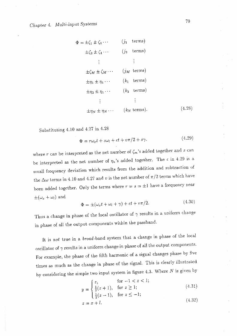
Chapter 4. Multi-inPut SYstems
(jt terms)
(j" terms)
(j¡a terms)
(kt terms)
(k, terms)
70
(4.30)
(4.31)
Õ:t(rt(t"'*(z t (r "'
:tnn,, + \¡¡ "' (kry terms)' (4.28)
Substituting 4'10 and 4'27 in 4'28
Q - ru,t* søt ¡ et I ur f2 * sl (4.2e)
where r can be interpreted as the net number of (-'s added together and s can
beinterpretedasthenetnumberof4,,'saddedtogether'Theein4'29isasmall frequency deviation which results from the addition and subtraction of
the Aø terms in 4.10 aú, 4.27 and u is the net number ol r f 2 terms which have
beenaddedtogether.ontythetermswhereT=s:tlhaveafrequencyneart(r' + ø¡) and
Q : !.(u,t* c¿¡ * l) t et t ur 12
Thus a change in phase of the local oscillator of 'y results in a uniform change
in phase of all the output components within the passband'
Itisr¿oútrueinabroail.bandsystemthatachangeinphaseofthelocaloscillator of .y results in a uniform change in phase of all the output components'
Forexample,thephaseofthefifthharmonicofasignalchangesphasebyflvetimes as much as the change in phase of the signal' This is cleariy illustrated
by considering the simple two input system in figure 4'3' where N is given by
for-l 1z<L;lor z 2l;lor z 1 -l;
,:{
L(urC¡ø"'!ry* nt"'Jrr¡zL?r".
l(z + t),
ä(' - r),z-x*1. (4.32)
7TChapter 4. Multi-inPut SYstems
II
+
+t
t_
Figure 4.3: A simple two input non-linearity. The nonlinearity, 'l{, is defined
by equation 4'32
Consider two d,ifierent cases. In the case of figure 4.4a, the sum of the signals
/ and r clearly exceed.s the linear range of N (equation 4.32)' In the case of
frgure 4.4b, the phase of /(t) has changed 180" and the sum of the signals / and
r clearly is within the linear range of N (equation 4.32). Thus, in this case the
distortion is very much dependent on the phase of the local osciliator system'
Note that this combination of signals and system does not fi't the extended
definition of bandpass systems in 4'1'
4.5 Summary
It was observed that mixer manufacturers' linearity specifications implicitly as-
sume a rather simple model of distortion in a two input device' This assumption
has been criticaliy examined and found to be invalid if the mixer does not have
a "pure"1 sinusoidal local oscillator'
1A distorted sinusoid is satisfactory since the distortion can be considered part of the
block N" in figure figure 4.1. A "broadened" sinusoid (perhaps due to amplitude or phase
modulation) is not satisfactorY'
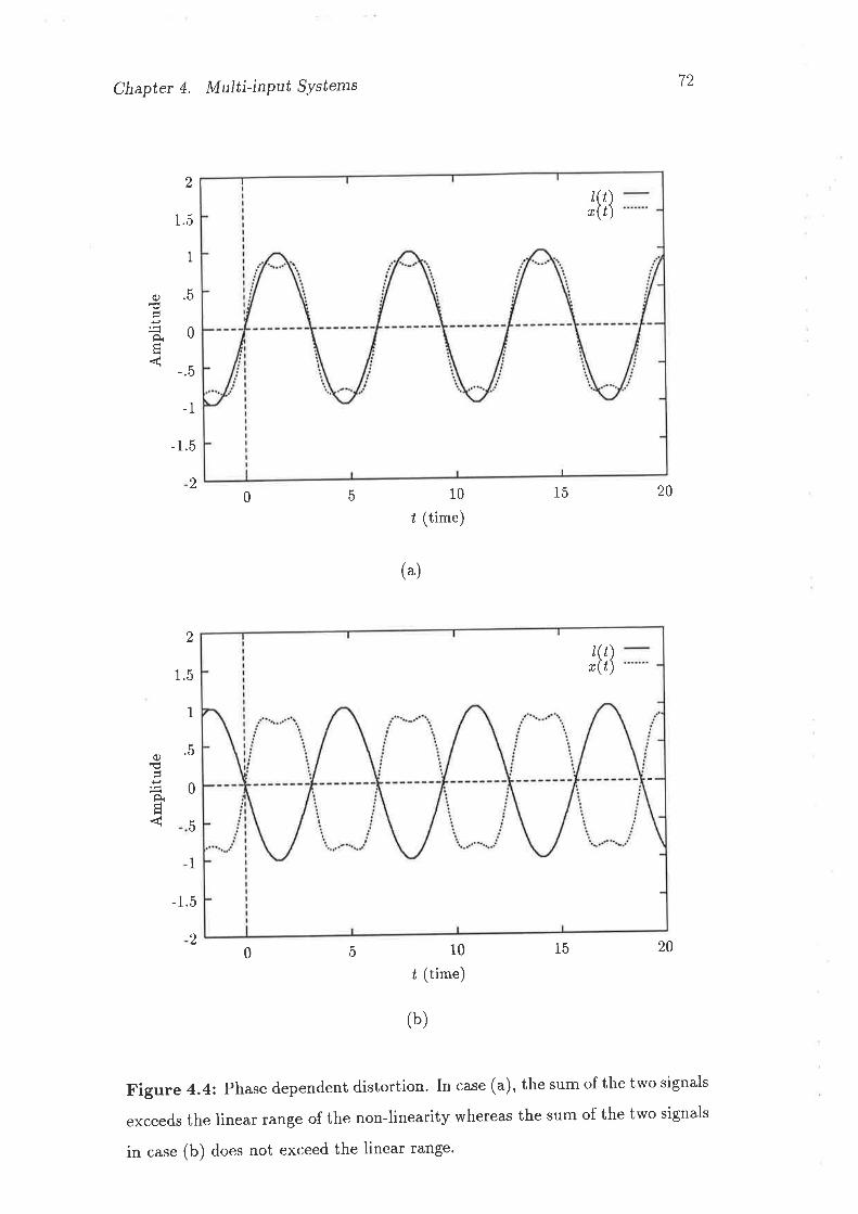
Chapter 4. Multi-inPut SYstems
5
1.5
-1.5
5
7.>
2
0)€
1.5
1
.5
0
-.5
-1
-1.5
20 10
f (time)15 20
20
(u)
2
1
.5
a€È 0
5
1
20 10
ú (time)
(b)
15
Figure 4.4: Phase dependent distortion. In case (a), the sum of the two signals
exceeds the linear range of the non-linearity whereas the sum of the two signals
in case (b) does not exceed the linear lange'
¿(¿)r(r)
/ (ú)r(¿)

Chapter 4. Multi-inPut SYstems73
Most mixer applications employ a sinusoidal local oscillator but some mod-
ern mixer applications use non-sinusoidal local oscillator signals such as a linear
frequency sweep (a "chirp") and caution must be exercised in applying pel-
formance measurements made with a sinusoidal local oscillator to these ap-
piications. It may be that a .'chirp" changed frequency slowly enough to be
consideredasinusoid,butthiswoulddependonthemixerandthefrequencysweep rate. The author speculates that useful relationships might arise from
studyingthecaseofconstantenvelopesignalsaslocaloscillators.
It was shown that in the case of a bandpass system, a change in phase of
one of the input signals results in the same change in phase of ali components of
the output signal within the passband. This result is of practical importance in
the modelling of d.istprtion in a receiver where it is impossible or impracticable
to measure the locai oscillator signals'
Chapter 5
Nonlinear Digital Filters
5.1- Introduction
Nonlinear digital fllters can be considered a discrete time version of the volterra
series discussed in section 3.4. Many of the concepts of linear digital filters can
be applied to nonlinear digital frlters. In particular, the thorny problem of esti-
mating the Volterra kernels can be performed "automatically" by an adaptive
nonlinear digital filter.
Nonlinear digital frlters can be used as predictors, estimators and equalizers
in the same way as linear digital frlters can be'
In this chapter we discuss the basis for nonlinear digital filters in the dis-
crete time Volterra series. We discuss a number of adaption algorithms and
their relative merits. Finally we discuss some of the features of a software
implementation.
74
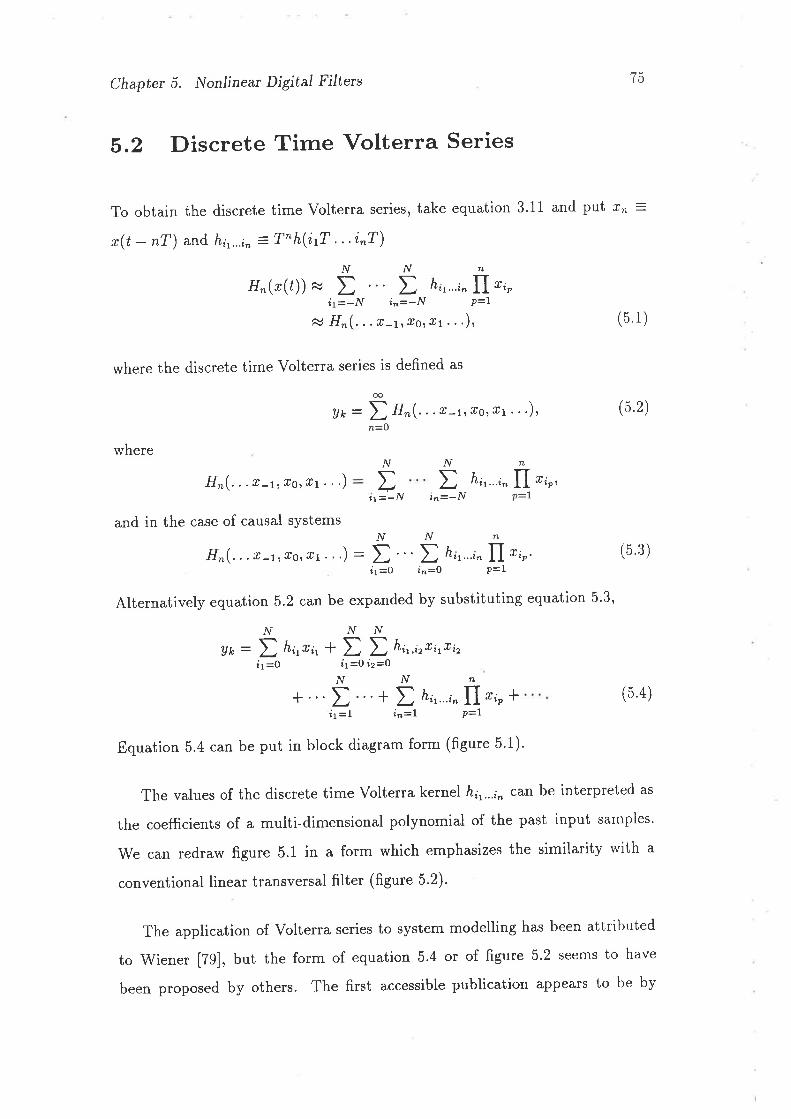
Chaptet 5. Nonlinear Digital Filterc IÐ
5.2 Discrete Time Volterra Series
To obtain the discrete time Volterra series, take equation 3.11 and put r,, :
r(t - n?) and hi,...i^ =T"h(i[ .. 'i"T)NNr"
H,(r(t))x D t h¿,'i^I.*noi1=-N i'=-N P=l
N H^(..'r -t,tro):tr...), (5'1)
where the discrete time Volterra series is defined as
Yk -- D H*(. ., t-r¡ Ïo¡rr'''), (5.2)oo
r¿=0
N N
where
and in the case of causal sYstems
H"(...lr-r,tÍo¡rr...)Nt
ll= -D hi,...i^1.*,o,N n
N i'=-N P=l
n
H.(...r-7¡r,o¡rr.") : t t hir...inl,*oo' (5 3)i1=O i¡=O P=l
Alternatively equation 5.2 can be expanded by substituting equation 5'3,
N
Ak:Dh¡rx¿r* h¿r,¿rr¿rr¿"l1=O i1 =O i2 =0
N N
NN
'D n
+ ..' t "'+ D hi,.,in|l,*,o + (5 4)i1 =1 i. =1 p=l
Equation 5.4 can be put in block diagram form (figure 5'1)'
The values of the discrete time Volterra kernel hir...in can be interpreted as
the coefficients of a multi-dimensional polynomial of the past input samples'
We can redraw figure 5.1 in a form which emphasizes the similarity with a
conventional linear transversal frlter (figure 5.2)'
The application of Volterra series to system modelling has been attributed
to Wiener [79], but the form of equation 5.4 or of figure 5.2 seems to have
been proposed by others. The first accessible publication appears to be by
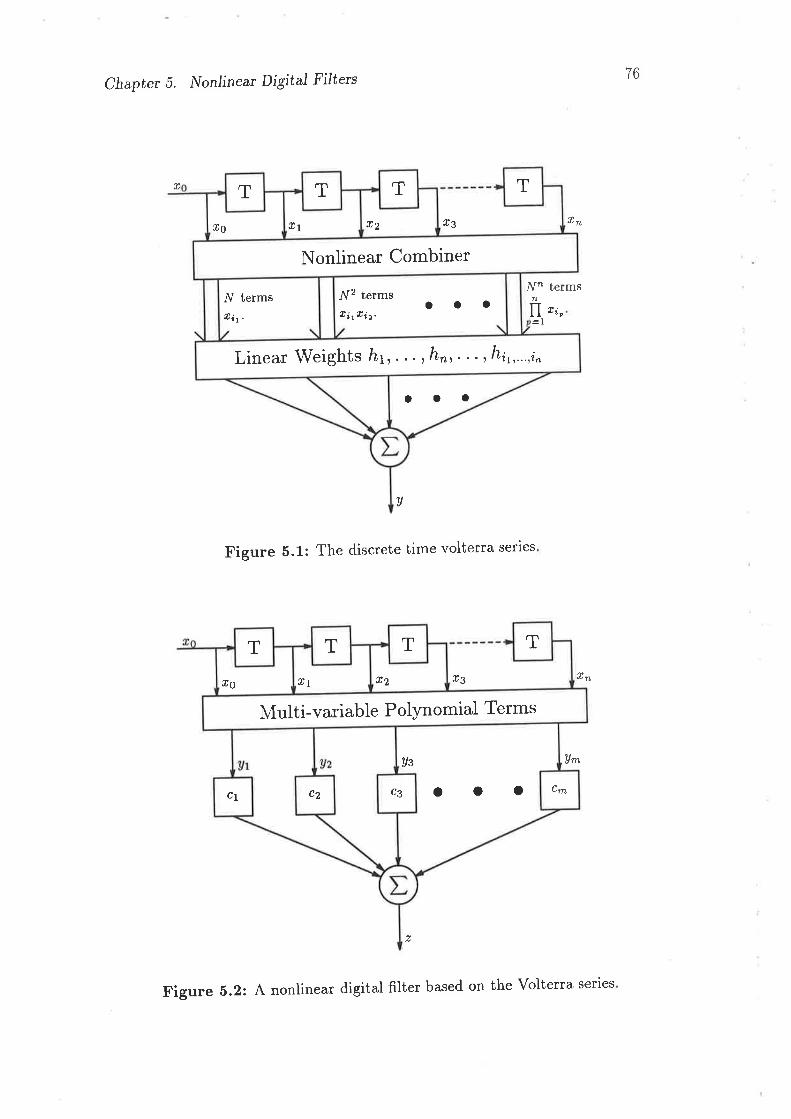
Chapter 5. Noniinear Digital Filters 76
r
r3 ln
N' termsn
fl 'to
a
Figure 5.1: The discrete time volterra series
r3 ln
Am
7
TTTTt2r1Og
Nonlinear Combiner
N2 termst itEiz'
aaaN termseit.
Linear \Meights ht,. . .,,hn,''',hir,'..,in
aao
TTTTr2r1rg
Multi-variable PolYnomial Terms
crncaC2Cy aaaUs
Figure 5.22 A, nonlinear digital filter based on the Volterra series
Chapter 5. Nonlinear Digital Filters 77
Gaborl [31]
The discrete time volterra series can be made an arbitrarily close approx-
imation to the continuous time Volterra series (equation 5.i) by increasing -fy'
and decreasing ?. As has been stated in chapter 3.4, any functional can be
arbitrarily well approximated over a given range by a continuous time volterra
series. It follows that any functional can be approximated arbitrarily well by a
discrete time Volterra series.
5.3 Nonlinear AdaPtive filters
The form of a digital frlter (linear or nonlinear) is relativeiy simple' The more
difficult problem is to determine the parameters of the digital filter so that it
has the desired characteristic.
Determining the volterra kernels from an analytic description of the distor-
tion is d.ifficult (and may not always be possible in "closed form")' Further,
in many applications, there might not even be an analytic description to start
from. These difficulties can be neatly circumvented by the use of adaptive
techniques [61].
There is some similarity between the nonlinear transversai filter (figure 5'2)
and a linear transversal filter. The linear case can be obtained as a special
case of the nonlinear filter by restricting the considering the "Multi-variable
Polynomial Terms" box of figure 5.2 to first order, in which case ai - ri'
For given y;, the variation of z as a function of c¿ is the same whether the
lTo quote Gabor: "It is difficult to say how much of this is new, as so much written on
the subject appears only in reports. From the abstracts circulated by the C'C'I'R it appears
that nonlinear filters operating on samples were frrst considered by H'E' Singleton in 1951'
and after him by w.D. white, also 1951, in reports of the General Electric co', schenectady
and of the Airborne lnstruments Lab., Mineola, respectively."
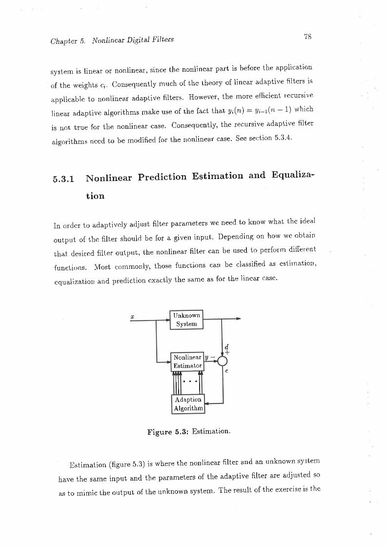
Chaptet 5. Nonijnea¡ Digital FilÚe¡s 78
system is linear or nonlinear, since the nonlinear part is before the application
of the weights c;. consequently much of the theory of linear adaptive filters is
applicable to nonlinear adaptive filters. However, the more efficient recursive
linear adaptive algorithms make use of the fact that y¿(n) : a¿-t'(n - 1) which
is not true for the nonlinear case. consequently, the recursive adaptive filter
algorithms need to be modified for the nonlinear case. see section 5'3'4'
5.3.L Nonlinear Prediction Estimation and Equaliza-
tion
In order to adaptively adjust filter parameters we need to know what the ideal
output of the fllter should be for a given input. Depending on how we obtain
that desired filter output, the nonlinear filter can be used to perform different
functions. Most commonly, those functions can be classifi'ed as estimation'
equalization and prediction exactly the same as for the linear case'
r
d+
e
Figure 5.3: Estimation.
Estimation (figure 5.3) is where the nonlinear filter and an unknown system
have the same input and the parameters of the adaptive filter are adjusted so
as to mimic the output of the unknown system. The result of the exercise is the
UnknownSystem
NonlinearEstimator
ilAdaptionAlgorithm
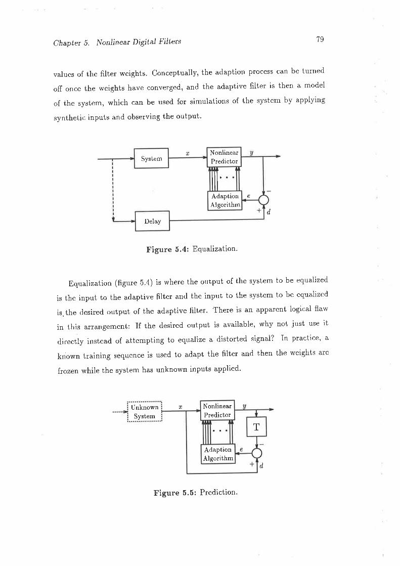
Chapter 5. Nonlinear Digital Filters 79
values of the filter weights. conceptually, the adaption process can be turned
off once the weights have converged, and the adaptive filter is then a model
of the system, which can be used for simulations of the system by applying
synthetic inputs and observing the output'
T
+ d
Figure 5.4: Equalization.
Equalization (figure 5.4) is where the output of the system to be equalized
is the input to the adaptive filter and the input to the system to be equalized
is. the desired output of the adaptive filter. There is an apparent logicai flaw
in this arrangement: If the desired output is available, why not just use ib
directly instead of attempting to equalize a distorted signai? In practice, a
known training sequence is used to adapt the filter and then the weights are
frozen while the system has unknown inputs applied'
UnknownSystem
n
d
NonlinearPredictorSystem
ïtïeAdaption
Algorithm
Delay
NonlinearPredictor
T
AdaptionAlgorithm
+
Figure 5.5: Prediction.
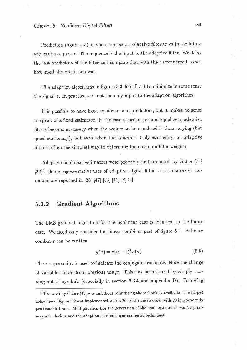
Chapter 5. Nonlinea¡ Digital Filterc 80
Prediction (figure 5.5) is where we use an adaptive filter to estimate future
values of a sequence. The sequence is the input to the adaptive filter. We delay
the last prediction of the filter and compare that with the current input to see
how good the prediction was.
The adaption algorithms in figures 5.3-5.5 all act to minimize in some sense
the signal e. In practice, e is not the only input to the adaption algorithm.
It is possible to have fixed equalizers and predictors, but it makes no sense
to speak of a fixed estimator. In the case of predictors and equalizers, adaptive
filters become necessary when the system to be equalized is time varying (but
quasi-stationary), but even when the system is truly stationary, an adaptive
filter is often the simplest way to determine the optimum filter weights.
Adaptive nonlinear estimators were probably first proposed by Gabor [31]
[32]2. Some representative uses of adaptive digital filters as estimators or cor-
rectors are reported in [2s] [47] [33] [11] [8] [9].
5.3.2 Gradient Algorithms
The LMS gradient algorithm for the nonlinear case is identical to the linear
case. We need only consider the linear combiner part of figure 5.2. A linear
combiner can be written
y(n) : c(n - 1).æ(rz). (5.5)
The + superscript is used to indicate the conjugate-transpose. Note the change
of variable names from previous usage. This has been forced by simply run-
ning out of symbols (especially in section 5.3.4 and appendix D). Following
2The work by Gabor [32] was ambitious considering the technology available. The tapped
delay line of figure 5.2 was implemented with a 20 track tape recorder with 20 independently
positionable heads. Multiplication (for the generation of the nonlinear) terms was by piezo-
magnetic devices and the adaption used analogue computer techniques.
Chapter 5. Nonlinear Digital Filters 8i
derivations do not make reference to previous sections of this chapter, so the
confusion should be minimal.
The error is defined
e(n):d(")-v(r),
and substituting equation 5'5, we get
e(n) : d(") - c(n - 1).æ(n)
(5.6)
(5 7)
Equation 5.7 defines the error before the coefficients have been updated'
After the coefficients have been updated, we can deflne a new error
ë.(n) : d(") - c(n)"æ(n), (5'8)
and a variant form,
e(n,k) : d(k) - c(n).æ(k)' (5.9)
We want to choose the value of c(rz) so as to minimize the mean squared value
oL ë(n,lc), 0 < k S n. The cost function to be minimized is
e(n) : iu(n,k)e(n,k).. (5.10)fr=0
We define the gradient of e(n) as
0e(n)
V [e(n)] :
0"t0e(n)Ô", (5.11)
ðe(n)ô"*
Differentiating equation 5.10 with respect Io c¿,,
W-: i :,-bh,k)ë(n,k).1a",@) - ?^ôc;(n)
t"\'
:Ëfr=0
oe nrk) ðë.(n, k é.(n,k)*0c¡(n)
ë(n,k)* -l0c;(n)
(5.12)
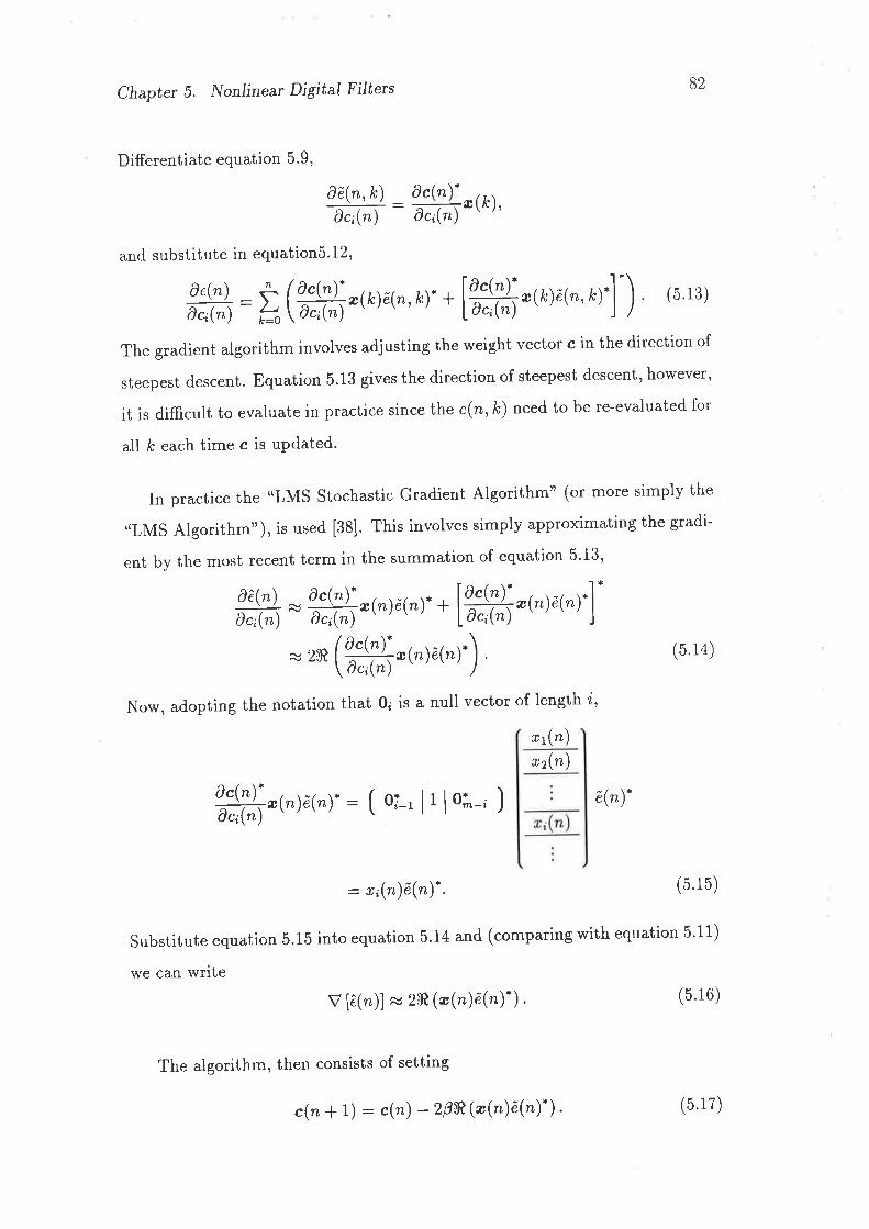
Chapter 5. Nonlinea¡ Digital Filters
Differentiate equation 5.9,
*(k),
82
(5.13)
\ë(n,k) - )c(n).
æ¿1"¡ - \c¿(n)
and substitute in equation5.l2,
ffi: å (Xffi''k)é(n'k).+ æ(k)é(n,*r.] )ôc(n).0c¡(n)
The gradient algorithm involves adjusting the weight vector c in the direction of
steepest descent. Equation 5.13 gives the direction of steepest descent, however,
it is difficult to evaluate in practice since the e(n,k) need to be re-evaluated for
all k each time c is uPdated.
In practice the "LMS Stochastic Gradient Algorithm" (or more simply the
*LMS Algorithm"), is used [38]. This involves simply approximating the gradi-
ent by the most recent term in the summation of equation 5'13,
ffi = Y*¡ * (n) ë (n)- * lYA,læ
( n ) a (' ). ]
=2ft(ffi,r,,)ã(n).) (5 14)
Now, adopting the notation that 0¿ is a null vector of length i,
x{n),r(r)
0c(n)-6@æ(n)a(n).: ( oi-, lt lo;-' ) ).e\n
: x;(n)ë(n).. (5'15)
substitute equation 5.15 into equation 5.14 and (comparing with equation 5'11)
we can write
V [ê(n)] ec 2ft (æ(n)ã(n).) . (5.16)
The algorithm, then consists of setting
c(n* 1) : c(n) -2|n(æ(n)e(n).) (5.17)
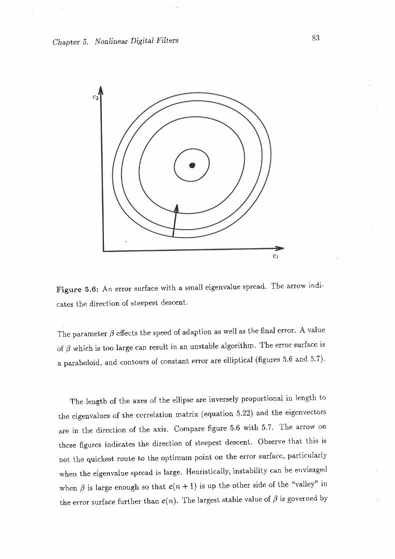
Chapter 5. Nonlinear Digital Filterc 83
c2
Figure 5.6: An error surface with a small eigenvalue spread. The arrow indi-
cates the direction of steepest descent'
The param eter B effects the speed of adaption as well as the final error' A value
of B which is too large can result in an unstable algorithm' The error surface is
a paraboloid, and contours of constant error are eiliptical (figures 5.6 and 5'7)'
The length of the axes of the ellipse are inversely proportional in length to
the eigenvalues of the ccrrelation matrix (equation 5.22) and the eigenvectors
are in the direction of the axis. compare figure 5.6 with 5.7. The arrow on
these figures indicates the direction of steepest descent. observe that this is
not the quickest route to the optimum point on the error surface, particularly
when the eigenvalue spread is large. Heuristically, instability can be envisaged
when B is large enough so that c(n * 1) is up the other side of the "valiey" in
the error surface further than c(n). The largest stable value of B is governed by
C7
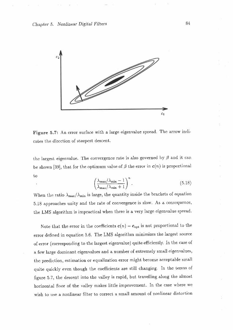
Chapter 5. Noniine¿¡ Digital Filterc 84
C2
Cy
Figure 5.7: An error surface with a large eigenvalue spread. The arrow indi-
cates the direction of steepest descent.
the largest eigenvalue. The convergence rate is also governed by B and it can
be shown [39], that for the optimum value of B the error in c(n) is proportional
to
lì'"*4ì"''" ' 1)". (5.18)\À-"*/À-i" + I /
When the ratio )-"*/À-i,, is large, the quantity inside the brackets of equation
5.18 approaches unity and the rate of convergence is slow. As a consequence'
the LMS algorithm is impractical when there is a very large eigenvalue spread.
Note that the error in the coefficients c(") - coo¡ is not proportional to the
error defined in equation 5.6. The LMS algorithm minimizes the largest source
of error (corresponding to the largest eigenvalue) quite efficiently. In the case of
a few large dominant eigenvalues and a number of extremely small eigenvalues,
the prediction, estimation or equalization error might become acceptable small
quite quickly even though the coefficients are still changing. In the terms of
figure 5.7, the descent into the valley is rapid, but travelling along the almost
horizontal floor of the valley makes little improvement. In the case where we
wish to use a nonlinear filter to correct a small amount of nonlinear distortion
Chaptet 5. Nonlinea¡ Digital Filterc 85
in the presence of a large undistorted (or linearly distorted) signal, then it is
necessary to allow the adaption to continue until the contribution due to the
small eigenvalues has been corrected. It is the ratio of the largest eigenvalue to
the smallest signifi,canú3 eigenvalue which is important'
The LMS Algorithm is very efficient in terms of arithmetic operations per
step. Referring to equations 5.5,5.6 and 5.17, there aren'¿ multiplications and
m - L additions to calculat e v(n),1 subtraction to calculate e(n) and m i I
multiplications and rr¿ additions to calculate c(n* 1). That is a total or.2mlI
multipiications, 2m - 1 additions and 1 subtraction per step'
5.3.3 Direct solution of the 'w'iener-Hopf Equations
A closed form expression for the optimum weights of a filter can be found'
Rewrite equation 5.13 as
ffi : mi a(,)e@, k). + lffi i æQe)e@. *).] (5.1e)
Thecoste(n)isminimizedbysettingm:0whichcanbeachievedif
læ(k)é(n, k)* = 0,TT
,t=0
(5.20)
(5.21)
and substituting equation 5.9 gives
læ(k)æ(k).c(n) : t æ(k)d(k).,n
&=0
n
fr=0
which is of the form
where
A(n)c(n) : a(n),
n
A(n) : ! æ(k)o(k)* : A(" - \ -t æ(n)æ'(n).
andË=0
sThe definition of "significant" varies with the application
(5.22)
Chaptet 5. Nonlinea¡ Digital Filúe¡s 86
n(n) : ir( ¡oç*). - o('- 1) + æ(n)d'(n)- ' (5'23)lc=0
Equation 5.21 (together with the definitions 5.22 and 5.23) is known as the
wiener-Hopf solution to the problem of minimizing equation D.17 [77]'
Direct solution of equation 5.21at every step is impractical, however there
is typically no need, to update c(n) at every n. The matrix .4 and the matrix
U must still be updated every step. some saving can be made by noting that
A(rz) is Hermitian. In the linear case, æ(n)*(r)* can be calculated relatively
efficiently by defining
A.a(rz) : æ(n)æ(n)*
and noting that the (i' j)th element is
L,a ¿,¡ (n) : r ¿(n) t i (n)*
:a¡-t¡-t(r- 1); i)0,7 > 0
(5.24)
(5.25)
Thus aÁ(n) can be updated with (rn - 1)2 copy operations and the new leading
row and column can be calculated wilh 2m - 1 multiplications. The matrix
A(n) can thus be updated with a total of (m - 1)2 copy operations ' 2n - |
multiplications and rn2 additions. For large m the rn2 additions and (m -1)2 copies dominate. If advantage is taken of the Hermitian nature of A(n),
and only upper (or lower) triangular sub-matrix of A(n) is stored, then the
number of operations can be almost halved. However, there is still m(m-l)12
additions, rn multiplications and (rn - 1)(- -2) 12 copies per step. Note that in
many computer implementations, copying takes of the order of the same time
as addition.
In the nonlinear case, the same idea for efficiently calculating A(n) can be
used since many of the nonlinear terms are delayed versions of other nonlinear
terms, but the actual operation count is dependent on the actual nonlinearity'
However, the number of operations is always more than the linear case, and
remains o(*r) per step or o(nm2) over n inputs. This excludes the operations
Chapter 5. NonJinear Digital Filterc 87
for the solution of equation 5.21 but assuming c(n) is updated infrequently the
time to calculate .4(n) is the dominant factor.
Direct solution of the Wiener-Hopf provides an exact least squares solutton'
Solution of a system of linear equations of the form 5.21 is a well understood
problem and robust algorithms such as the QR method [25], or singular value
decomposition [26] are available as library routines. These routines are well
behaved even in the face of relatively poorly conditioned matrices (which cor-
responds to a large eigenvalue spread).
5.9.4 Recursive Least Squares Algorithms
Gradient algorithms (section 5.3.2) work well when the eigenvalue spread is
small. Direct solution of the Wiener-Hopf equations gives a true optimum
over the samples input with no convergence time required and when a suitable
method is used to solve the equation, accurate results can be achieved even when
there is a large eigenvalue spread. However, the execution time (and storage
requirements) scales as o(nm2) and when a large number of taps is required
the computation becomes excessive.
A variety of algorithms have emerged which have a range of compromlses
between convergence rate, final error rate, robustness and computational com-
plexity. Lattice algorithms perform well on many of these counts [40]' but
cannot be used unmodified to model general nonlinear systems' A class of al-
gorithms known as Recursive Least Squares (RLS) have been invented which
recursively calculate the true least squares weights. In rn steps an rnth order
weight vector can be calculated [52]. RLS algorithms exist in both transversal
and lattice forms [41] [51] l22l 148]. None of these algorithms can be applied
directly in the nonlinear case.
The linear RLS algorithms achieve computational efrciency by making use
Chapter 5. Non/inea¡ Digital Fi/te¡s 88
of. a priori information about the nature of the inputs to the linear combiner'
In particular, if the filter is defined bv y(") - c*æ(n), then the linear RLS
algorithms make use of the fact that the elements o1æ(n * 1) are simply those
of æ(n) shifted along, with the last element removed and a new first element'
To extend these algorithms to the nonlinear case, we need to similarly take
advantage of any a priori information on the nature of the elements of æ. To
do that we cast the nonlinear filter in a form of a filter operating on vector
(instead of scalar) inputs. For example the terms of a nonlinear filter might be
defined as where r¿ is the input x(t - ff). At the next sampling instant, all
è ès21
delay --+€r Ên € 5 €6
r1I1IyI1r1fr1t2I11212r112t3
r2I21212r2:D2t3f 2tgI3r2r314
r3rgf 3Jt3I3t314IgÍ414rstars
r,4
t41414f 4t4rgf 415f g
t4Igt6
t5Igf 5lt5rgtsr6f 5f 616r51617
I6I616r'6r,616f 7
r6ü7I71617rg
Figure 5.8: organization of nonlinear terms into column vectors.
the columns vectors shift right so that €,(r) : €r-t(" - 1). If the nonlinear
filter can be put in the form of figure 5.8, then the algorithms developed in
[b1] are directly applicable. It is would also be a relatively straight forward
exercise to convert other algorithms such as those in l22l [a8] to operate on
vector quantities. Unfortunately, a nonlinear frlter can't in general be put in
the form of figure 5.8. Note that, in figure 5.8, there are third order terms with
delays of up to 8 samples whilst the linear terms have a maximum delay of 6
sampies. Ideally, we would like to be able to have different ranges of delay for
each order. Typically, a system model has fewer significant high order terms
than low order terms and so a more applopriate model \4/ould be of the form
of flgure 5.9. The problem with this form is that the length of the vectors {;
varies with i. The author has derived an algorithm for an RLS Transversal
Filter and an RLS Lattice Filter operating on the representation in figure 5.9'
Chapter 5. NonJinea¡ Digital Filters 89
€'€delaY
-rêcs3 s4 èÈss s62
I1r,11111I111t2I112f 2
r112î3
&2
r21212I21213r21313
I3rgtgI3
J'4 l5 r6
Figure 5.9: Organization of nonlinear terms into column vectors'
The particular RLS Transversal Filter derived is known as the "Fast Kalman"
filter. The method is based on that of Mueller [5i], but allowing the length of
{¿ to vary with i complicates the algorithm (and its derivation) considerably.
The derivation is lengthy and so has been consigned to appendix D' Here we
will discuss only the the formulation of the problem and the over all strategy.
The author implemented a linear version of the Fast Kalman algorithm tn
software and it was found to be numerically unstable. Errors due to finite
precision effects increase exponentially with time. This experience has been
confirmed in the literature. Cioffi and Kailafh 122) develop a number of im-
provements to alleviate the problem. The Lattice filter, on the other hand
appears to be much more robust. Since the extension to nonlinear filters is
likely to be at least as susceptible to these problems, we will concentrate on the
lattice filter. The nonlinear Fast Kalman algorithm has been developed in ap-
pendix D principally because it is little extra effort since much of the derivation
is common to both the RLS Lattice Algorithm and the Fast Kalman algorithm'
Strategy
The vector of inputs to the linear combiner is defined in equation D.1 by
æ*(n)*: ( €,{"). l€r{'r). l...lg-("). ) . (5.26)
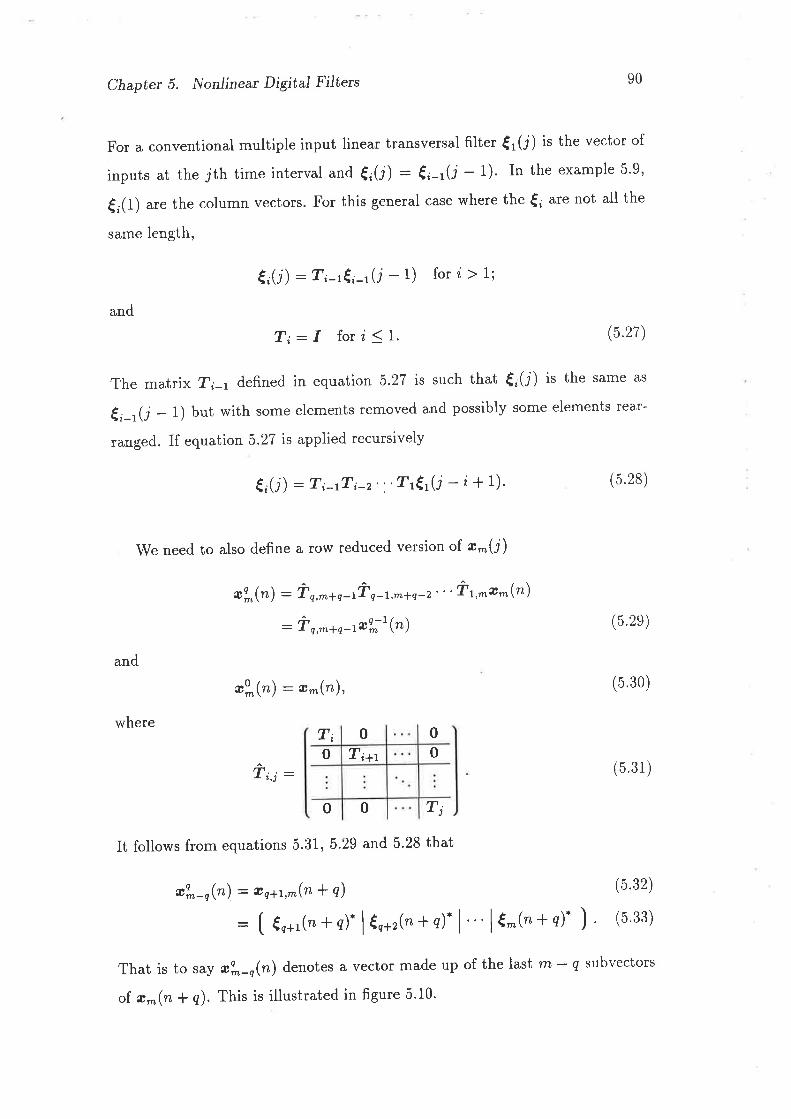
Chapter 5. Nonlineat Digital Filterc 90
For a conventional multiple input linear transversal filter €t(i) it the vector of
inputs at the jth time interval and {¡(j) : €;-r(r - 1). In the example 5.9,
{¿(1) are the column vectors. For this general case where the {¿ are not all the
same length,
€¿(r) : T;-t€¿-tU-1) fori > 1;
and
T;:I fori(1. (5.27)
The matrix T¿; defined in equation 5.27 is such that {;(j) is the same as
€,r_r(j - 1) but with some elements removed and possibly some elements rear-
ranged. If equation 5.27 is applied recursively
€;(r) : T¿-tT;-2".'Tt€4(i - i + 1). (5.28)
We need to also define a row reduced version of æ^(j)
and
*î,(") - Û q,,n*ø-tf n-r,^+n-2''' ù 1,^æ^(n)
: Ûq,^+q-rælit@)
,o*(") - æ^(n),
(5.2e)
(5.30)
(5.3 1 )
where
Ì;,j:
T¡ 0
0 0
000
T¡
It follows from equations 5.31, 5.29 and 5'28 that
!^('*q). ) ll liì
That is to say g.l^_n@) denotes a vector made up of the last nx - q subvectors
of. æ^(n + ø). This is illustrated in figure 5'10'
T;+t
Chapter 5. Non.linear Digital Filters 91
-0úm-l
æ?n
aL-t
ès1
èT2
¿s3
o
o
O
€m-r
c('m
ès1
ès2
ès3
o
o
o
€--r
èt2
ès3
o
o
a
€--r
èm
Figure 5.10: Reduced order filter "taps"
Chapter 5. Nonlinear Digital Filters 92
The method basically involves finding time and order recursive relationships
for the various filter parameters. The time recursive relationships arise from
the recursive forms for equations 5.22 and 5.23. Two order recursive forms are
needed. One is derived by reducing the order from the right and the other is
derived by reducing the order from the left (figure 5.10)' Thus we describe
the parameters of the filter based on æfr(n) in terms of the parameters of the
filters based on to^-r(n) and æt^-r(, - l). The main reason for the increased
complexity of the derivation of the nonlinear version of these algorithms, is that
in the linear case, æl_r("- 1) : æo^-r(n- 1). In the linear case we can describe
a mih order filter in terms of parameters of the (rn - l)th order filter and the
delayed parameters of (rn - l)th order filter. In the nonlinear case we need
to maintain filters with values of rn and q of (1, rt1,1 - l),(2,rrr1 - 1), (3' rn1 -2)...(*r,0)inorderforthefinalfiltertohaveQ:0andrn-nÙl.Theprocessis illustrated in figure D.4. In section D.10 we demonstrate that much of this
computational burden can be removed if some of the ùq,^+ø-r: .f. The more
efficient method is illustrated in figure D.5. For the application of identifying a
system with only small nonlinear distortion in the presence of significant linear
distortion, it will often be the case thal Ìq,^+q-7 : f for large nz. For m in
this region, the computational burden increases as O(nm)'
Verification
with a derivation as lengthy as that in appendix D, it is difficult to be confi-
dent that their are no errors. To gain confidence in the derivation a verifica-
tion process was performed. This was done using a "programmable calculator"
programa. This program has a significant number of built in matrix operations'
Programs (calc macros) where written to evaluate the filter parameters for
a range of rn and n using straight forward methods. For both the forward
aThe program is called calc by David Gillespie and is written in GNU emacs lisp
Chapter 5. Nonlinear Digital Fi/te¡s 93
and backward predictor case, matrix.á. is evaluated using equation D.24,, u"
is evaluated using equation D.25, d" is evaluated using equation D.12, c" is
calculated by solving equation D.23 using the built in matrix inversion function,
the error e" is calculated using equation D.13, €s was calculated using equations
D.34 and D.35, the Kalman gain g was calculated from equation D.38, and ã"
was calculated from equation D.15, and lcl was calculated using equation D.148.
All these parameters were evaluated for 1 < n < 10 and rn :2,3 and q : 0, 1'
These parameters were then substituted both sides of equations D.167, D.168'
D.191, D.L92,D.207 and D.216 and checked for equality.
Essentially, we have used the method of direct solution of the Wiener-Hopf
equations (section 5.3.3) plus some auxiliary equations to verify the order re-
cursive relationships of the RLS algorithms.
5.4 Orthogonalization
The recursive least squares algorithms perform a partial orthogonalization of
the ø vector (see section D.3) and the high performance is attributable to this.
Also, the better algorithms for direct solution of the Wiener-Hopf equation
perform orthogonalization.
It is possible to perform this orthogonalization explicitly by replacing the
nonlinear box in figure 5.2 with one which has orthogonal outputs. Then the
coefficients could be evaluated by correlation or by the gradient algorithm (the
maximum convergence rate would be much increased), The question arises of
how to determine the contents of the nonlinear box which would have the or-
thogonal outputs required. One approach is based on having a priori knowledge
of the probability density function of the input. This is the approach used in
the Wiener models discussed in section 3.5 and has the disadvantage that the
sThe orthogonalization in the Wiener model is actually performed in two stages'
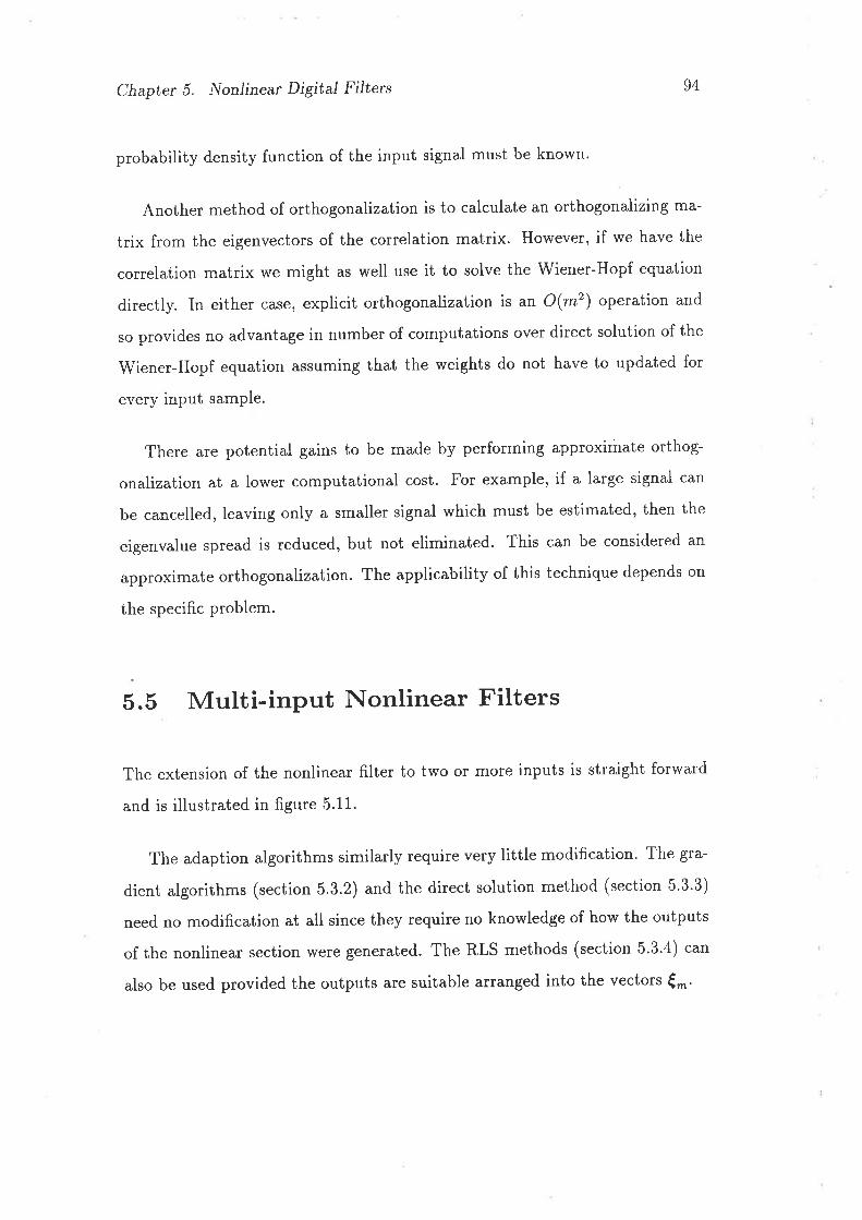
Chapter 5. NonJinear Digital Filtets
probability density function of the input signal must be known.
Another method of orthogonalization is to calculate an orthogonalizing ma-
trix from the eigenvectors of the correlation matrix. However, if we have the
correlation matrix we might as well use it to solve the Wiener-Hopf equation
directly. In either case, explicit orthogonalization is an O(rn2) operation and
so provides no advantage in number of computations over direct solution of the
Wiener-Hopf equation assuming that the weights do not have to updated for
every input sample.
There are potential gains to be made by performing approximate orthog-
onalization at a lower computational cost. For example, if a large signal can
be cancelled, leaving only a smaller signal which must be estimated, then the
eigenvalue spread is reduced, but not eliminated. This can be considered an
approximate orthogonalization. The applicability of this technique depends on
the specific problem.
5.5 Multi-input Nonlinear Filters
The extension of the nonlinear filter to two or more inputs is straight forward
and is illustrated in figure 5.11.
The adaption algorithms similarly require very little modification. The gra-
dient algorithms (section 5.3.2) and the direct solution method (section 5.3.3)
need no modification at all since they require no knowledge of how the outputs
of the nonlinear section were generated. The RLS methods (section 5.3.4) can
also be used provided the outputs are suitable arranged into the vectors {-'
94
T
o Â, È + o B S¡ z o o Þ I F. + $, +j o I fD
r2&
nIz A^
Figu
re 5
.11:
A tw
o in
put n
onlin
ear
filte
r ba
sed
on th
e vo
lterr
a se
ries
In
t
(o C^
T
c1n
T1I
T
oI
aoo
Ae
C3
T
c2C
1
TI1
Trg
Mul
ti-va
riabl
e P
olY
nom
ial
Term
s
Chapter 5. Nonlinear Digital Filtets 96
5.6 Implementation Considerations
5.6.1 Initialization
Regardless of the algorithm used, the question arises what to initialize the delay
iine of figure 5.2 to at time t : 0. If we have no information about how the
input behaves prior to this time, then initializing the delay line to zero seems
as good as any, however it is certainly not the only strategy possible. In the
experiments which are described in chapter 6, the signals are all periodic' In
these circumstances it is possible to do much better than initialization with
zero,
In the software implementation of the direct solution method (section 5'3'3)
written for the experiments in chapter 6 an option was included to aliow the
delay line to be pre-loaded. If pre-loading was specified, the input data was
cycled through once to initialize the delay line and a second time to calculate
,4(n) and o(n) according to equations 5'22 arrd 5'23'
5.6.2 Software
A suite of programs wele developed to implement and test nonlinear adaptive
filters. Data files were organized so that the first four bytes contained a magic
number indicating whether the rest of the file contained integers, floating point
numbers, complex floating point rrumbers etc. The absence of a valid magic
number indicated an ascii file. This feature proved invaluable (once the input
and output library was written) since short tests could be conducted with data
created with a text editor but a more efÊcient binary representation was used
when large amounts of data had to be processed. Each program had an op-
tion for specifying binary or ascii output. In the case of binary output, some
programs output integers and others output floating point numbers and others
Chapter 5. Nonlinear Digital FiJúe¡s 97
output complex floating point numbers. In any case, the appropriate magic
number would be output first so that other programs in the suite would be able
to properly interpret the data. In many cases, the output of one program would
be fed into another program via a UNIX pipe avoiding the need for a temporary
disk file.
The suite consisted of programs to generate random test data, perform linear
combinations of two streams, perform arbitrary nonlinear filtering operations,
calculate the mean squared difference between two streams and calculate opti-
mum filter weights. The nonlinear filter and the weight calculation programs
were able to take an arbitrary number of inputs (up to some maximum depen-
dent on a system imposed limit on the number of open files).
The Nonlinear Filter Program
The weights of the nonlinear filter are specified by a parameter file which con-
tains entries of the form
{rytuple, n2tuple, ...,n;tuple} value
where n¿tuple is of the form
{d;,r, d¿,r, . . ., d;,nr}
where d;,¡ is the ith input delayed by j and value is either a real number or a
complex number written as {real,imag}. for example, the entry
{{4,4}, {4}} {0,0.7}
indicates that inputl,a x inputr,n x inputz,4 has the complexweight 0+0.7i
Internally, the history of each input is kept in an array. At each sample
instant, the elements of the input arrays are all shifted one position and a nelv
element is read into each one. Each weight has associated with it a list of
Chapter 5. Nonlinear Digital Filtets 98
pointers to elements in the input arrays. Thus the nonlinear product terms are
simply created by de-referencing each of the pointers in the list and forming
a running product. This does involve some redundant calculations since many
product terms will have common sub-expressions. These could probably be
eliminated by constructing a tree of all the multiplications to be done'' but care
needs to be taken to ensure that the more complex code doesntt take longer
than the operations saved' This is machine dependent'
The'Weight Calculation Program (Direct Solution)
The weight calculation program calculates the nonlinear products in a similar
mannel to the Nonlinear Filter program. Howevet, the specification of the
product terms is somewhat different. The product terms are specified in a
parameter file which has elements of the form
tupler, tuple2, '.., tuPlen canon
where tuple¡ is of the form
{order,max. delaY}'
The úuple¿ represents the products of orde¡ using delays from zero up to max'
delayfor the ith input. The program automatically works out all the possible
products across all the inputs specifred' The canon field is used to optionally
indicate that additional terms be included which are the product of the inputs
indicated by the rest of the entry with all terms delayed by the same amount
up to canon.
For examPle, an en
following terms (which
{ {0, 0},{{1,1},{{1,0},{{2,1},{{2,0},
try in the parameters file of {2,3},{1,1} results in the
are in the form discussed in section 5'6'2 above):
{0} }{1} }{0} }{1} }{0} }
{{3,1},{{3,0},
{{3,2},{{3,1},{{2,2},{{3,3},{{3,2},
{{3,3}, {o}}{{0, o}, {1}}{{1, o}, {1}}{{2, o}, {1}}{{3, o}, {1}}.
{1}}{0} }{0} }{1}}{0} }
{0} }{0} }
{1} }
{1}}{{1{{2{{2
, 1),,2\,, 1), {0} }
Chapter 5. Non/inear Digital Filters 99
The number of terms clearly increases very rapidty with otder, max' delay
and number of inputs. The canon field was introduced in the expectation that
a delayed terms of the canonical form might be more significant' As an example
of a parameter entry using the canon field fleld, an entry in the parameters file
of
results in the following terms:
Once the nonlinear products have been calculated, the calculation of the
matrix A(n) and the vector 1'(rz) is performed using the copying optimization
discussed in section 5.3.3. with the aid of Linpack library routines, the solution
oT the wiener-Hopf equations is straight forward. Both QR and svD algorithms
were tried. see sections 6.4.3 and 6.5.2 for discussion on the suitability of the
SVDalgorithmfortheparticularcaseoftheHFRexperiments.
The Weight Calculation Program (Recursive Least Squares)
A functional implementation of the RLS algorithm has not been completed,
however, as far as external inputs are concerned, it is designed to appear the
same as the program implementing the direct solution method' one exception
is the ,,pre-loading,' feature which was easily implemented for the direct solution
method (section 5.6.1). It is not straight forward to initialize the RLS method
in the same way
91){2,3}, {1
{{7,7},{{o, o},{{8,8},i{1,1},
{{3,1},
{0} }{1}}{2} }{3} }{4i }{5} }{6} }
{0}{0}{1}{0}{1}{0}{0}
{{3,0}{{1,1}{{2,2}i{2,1}{ {3, 2}
{{3,1}{{2,2}
{7}}{s} }{e} }{0} }i1ÌÌ{0} }{1}}
)))ÌÌÌ)
{{3,2},{{3,3i,
i{3,3},
{{0,0},{i1,0}{{2,0}{{3,0}
{1}}{0} }{0}}{1}}{1}}{1}}{1}}
u2,2\,{ {3, 3}{{4,4}{{5,5}{{6,6}
{ {9, 9},{i1,0},i{2,1},{{2,0},
It is worth noting that the elements of the sub-vectors f, can always be
Chaptet 5. Noniinear Digital Filters 100
ordered in such a way that the matrix in is of the form
ùo= (rlo ) (5.34)
If i]o is of the form of equation 5.34, expressions of the form
ùî (ù,,';\'(, - 1)f;)-'rn, (5'35)
which appear in a number of equations in the RLS Lattice algorithm (section
D.10), is equivalent to inverting a pqrr xPq+r sub-matrix of ,k\t and zeroing
the elements outside this sub-matrix. This is clearly a much cheaper operation
than a naive evaluation of expression 5.35. Indeed, it turns out that the ? and
!i' don,t need to ever be stored. Alt that needs to be stored are the values of
p¿..1 which are the number of rows of the ? matrices'
5.7 Summary
In this chapter, we have discussed the theory and implementation of adaptive
nonlinear digital filters. we have seen how the discrete time volterra series can
form the basis for a nonlinear digital filter. Nonlinear filters can be made to
adapt to a required characteristic. The nonlinear adaptive filter can be used
in the roles of estimators, predictors and equalizers in the same way as linear
adaptive filters.
The LMS gradient algorithm and the method of directly solving the wiener-
Hopf equations used in linear adaptive filters are directly applicable to the non-
linear case. other more efficient linear adaption algorithms such as the Recur-
sive Least squares algorithms are not directly applicable to the nonlinear case'
The Recursive Least Squares algorithm has been extended to the nonlinear case
in section 5.3.4. The LMS gradient algorithm and the RLS algorithm require
O(nm) operations, whereas the Direct Solution of the Wiener-Hopf equations
requires o(nm2) operations assuming that the weights are updated infrequently
Chapter 5. Nonlinear Digital Filters 101
so that number of operations is dominated by the calculation of the correlation
matrix A. The RLS algorithms and direct solution of the Wiener-Hopf equa-
tions have zero convergence time.
RLS algorithms achieve their efficiency by partial orthogonalization of the
nonlinear product terms. It is possible to explicitly orthogonalize the outputs of
the filter's nonlinear combiner which has the potential to improve convergence
rates. However, explicit orthogonalization has no computationai advantage over
direct solution of the wiener-Hopf equations assuming that the weights do not
have to updated for every input sample'
The single input nonlinear digital filter is simply extendibie to two or more
inputs. The adaption algorithms can also be extended to the multi-input case'
The performance of adaption algorithms in the presence of periodic signals
can be improved by appropriate initialization of the filter. The implementation
of a suite of programs for efficiently implementing and testing nonlinear adaptive
filters has been discussed'
Chapter 6
HFR Receiver Experiments
6.1 Introduction
Workers in High Frequency Over the Horizon Radar (HF OTHR) have been
interested in high linearity RF equipment for some time l2l l27l [17]. The per-
formance of all the RF equipment is, of course, important, but the receivers
are possibly the most critical in terms of nonlinear performance, since they are
exposed to large signals (interference) over which the radar designer has no
control. Anderson [2] notes the Volterra Series is a general way of representing
the receiver output, but is forced to simplify the model considerably in his sim-
ulation. In particular, the system is assumed to consist of distortionless mixers,
ideal filters and amplifiers which are memoryless nonlinearities. The nonlinear
parameters were estimated by comparing the intermodulation distortion of the
model and of a real receiver with a two tone test. As has been pointed out
(section 3.7), a two tone test is not capable of identifying a general nonlinear-
ity. Eart [27] used an even simpler model, the power series, in his study of
cross-modulation effects.
Accurate models of receiver nonlinearities would allow better simulation of
r02
Chapter 6. HFR Receiver Experiments 103
the actual radar performance attainable in a particular HF environment' If such
simulations reveal that the best receivers have distortion levels which limit radar
performance, then it is of interest to know to what extent receiver nonlinearities
can be improved by post processing. Modelling and correction correspond to
estimation and equalization discussed in section 5'3'1'
The aim of the experiments of this chapter are to see how well, in practice,
adaptive nonlinear digital filters can be used to estimate and equalize distortion
in an HFR receiver. we are also able to verify experimentally the theoretical
properties of multiple input systems derived in chapter 4'
Similar experiments which use adaptive nonlinear digital filters of the form
described in chapter 5 to model or correct distortion in reall systems have been
described in the literature [28] [47] tgl [1]'
The HFR receiver has some properties which mean the design of the exper-
iment must differ significantly to other experiments described in the literature'
Specifically:
1. The receiver must be modelled as a two input device'
2. The receiver has slight, but important, nonlinear distortion in the presence
of large linear distortion.
3. The receiver's inputs and outputs are at diferent frequencies'
4. The band width of the signals applied to the receiver's inputs should be
very much greater than the band width of the receiver output.
These features, and the reason they affect the experiment are discussed in sec-
tions 6.2 and 6.3.
lln some cases the authors do not make it clear whether they are dealing with a real
system or a simulation. In the case of simulations, there are simulations of real systems and
simulations of hypothetical systems so the classification becomes fuzzy.
Chapter 6. HFR Receiver Expeúments 104
These experiments presented some non-trivial problems in the generation of
test signals, selection of sampling rates and design and implementation of the
analysis algorithms.
6.2 The HFR Receiver and Its operating
Conditions
The Jindalee2 stage B receiver is a triple conversion heterodyne design man-
ufactured by sRI International. The receiver used in the experiments of this
chapter was not an actual stage B receiver, but an experimental version which
had several modules replaced. Most notably, the output band width of the re-
ceiver had been increased. A block diagram of the receiver is shown in flgure
6.1.
In normal operation, the first local oscillator is a continuous FM signal
where the modulating signal is a linear sweep continuously repeated (a saw
tooth). This results in a sequence of "chirps". We will refer to this signal as
an FMCW signal. The other local oscillators are sinusoids' The receiver input
consists of noise, interference, ground clutter, sea clutter and (moving) targets
all transformed by reflection from the ionosphere which might include significant
multipath effects. The signal from ground clutter, sea clutter and target signals
must be of the form of an infinite sum of delayed (and possibly doppler shifted)
versions of the transmitted signal which is also an FMCW signal. A discussion
of the theory ofoperation ofradars is outside the scope ofthis thesis, but see [46]
[3]. The largest source of interference under normal circumstances is AM HF
broadcast stations. Of course, in the case of deliberate interference (jamming)
the nature of the interference can't be predicted and is likely to be of the most
troublesome nature.
2The Australian OTHR facilitY [2]
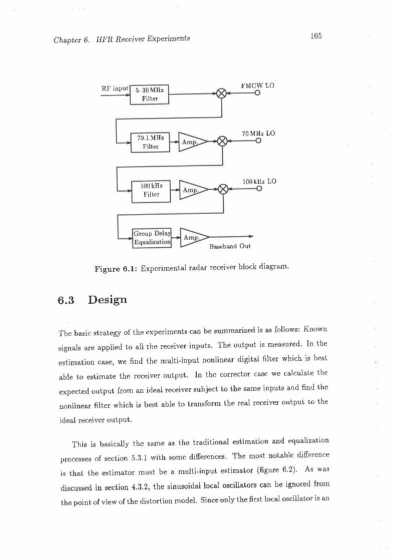
5-30 MHzFilter
70.1MHzFilter
100 kHzFilter
Group
Chapter 6. HFR Receivet Expeúments 105
RF input FMCW tO
70 MHz LO
100kHz LO
Baseband Out
Figure 6.1: Experimental radar receiver block diagram
6.3 Design
The basic strategy of the experiments can be summarized is as follows: Known
signals are applied to all the receiver inputs. The output is measured' In the
estimation case, we find the multi-input nonlinear digital filter which is best
able to estimate the receiver output. In the corrector case we calculate the
expected output from an ideal receiver subject to the same inputs and find the
nonlinear filter which is best able to transform the real receiver output to the
ideal receiver outPut.
This is basically the same as the traditional estimation and equalization
processes of section 5.3.1 with some differences. The most notable difference
is that the estimator must be a multi-input estimator (figure 6.2). As was
discussed in section 4.3.2, the sinusoidal local oscillators can be ignored from
the point of view of the distortion model. since only the first local oscillator is an
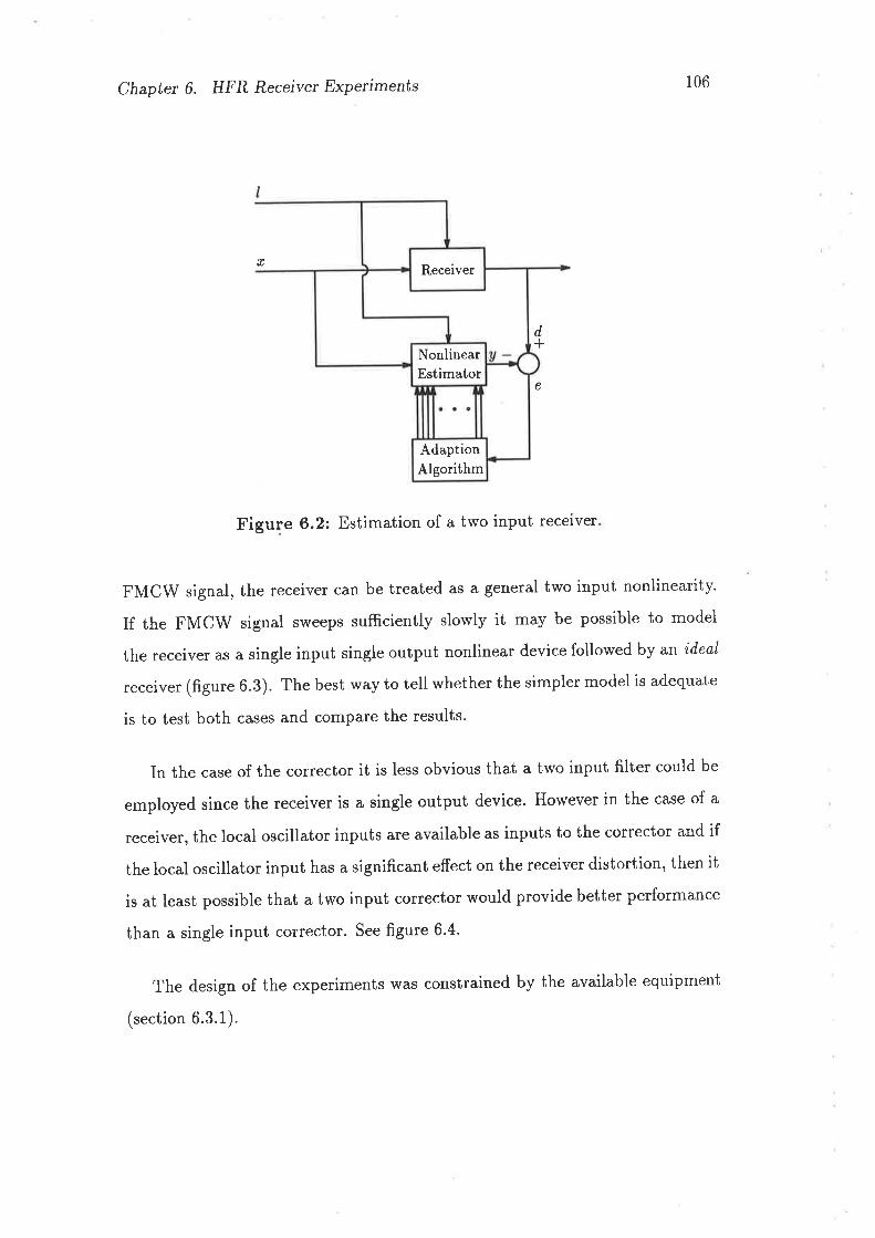
Chapter 6. HFR Receiver Experiments 106
Figure 6.2: Estimation of a two input receiver
FMCW signal, the receiver can be treated as a general two input nonlinearity.
If the FMCW signal sweeps sufficiently slowly it may be possible to model
the receiver as a sìngle input single output nonlinear device followed by an ideal
receiver (figure 6.3). The best way to tell whether the simpler model is adequate
is to test both cases and compare the results.
In the case of the corrector it is less obvious that a two input filter could be
employed since the receiver is a single output device. However in the case of a
receiver, the local oscillator inputs are available as inputs to the corrector and if
the local oscillator input has a significant effect on the receiver distortion, then it
is at least possible that a two input corrector would provide better performance
than a single input corrector. See figure 6.4.
The design of the experiments was constrained by the available equipment
(section 6.3.1).
T
d+
e
Receiver
NonlinearEstimator
AdaptionAlgorithm
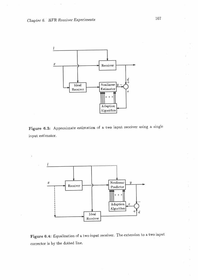
Chapter 6. HFR Receiver Expeúments 107
Figure 6.3: Approximate estimation of a two input receiver using a single
input estimator.
Figure 6.4: Equalization of a two input receiver' The extension to a two input
I
r
d+
e
r
d
Receiver
NonlinearEstimator
IdealReceiver
AdaptionAlgorithm
NonlinearPredictorReceiver
AdaptionAlgorithm
IdealReceiver
corrector is bY the dotted line.
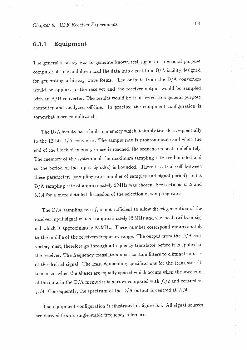
Chapter 6. HFR Receiver Expeñments 108
6.3.1 Equipment
The general strategy was to generate known test signals in a general purpose
computer off-line and down load the data into a real-time D/A facility designed
for generating arbitrary wave forms. The outputs from the D/A converters
would be applied to the receiver and the receivet output would be sampled
with an A/D converter. The results would be transferred to a general purpose
computer and analyzed off-line. In practice the equipment configuration is
somewhat more comPlicated.
The D/A facility has a built in memory which it simply transfers sequentially
to the 12 bit D/A converter. The sample rate is programmable and when the
end of the block of memory in use is reached, the sequence repeats indefinitely.
The memory of the system and the maximum sampling rate are bounded and
so the period of the input signat(s) is bounded. There is a trade-off between
these parameters (sampling rate, number of samples and signal period), but a
D/A sampling rate of approximately SMHz was chosen. See sections 6'3'2 and
6.3.4 for a more detailed discussion of the selection of sampling rates'
The D/A sampling rate /" is not sufficient to allow direct generation of the
receiver input signal which is approximately 15 MHz and the local oscillator sig-
nal which is approximately 85 MHz. These number correspond approximately
to the middle of the receivers frequency range. The output from the D/A con-
verter, must, therefore go through a frequency translator before it is applied to
the receiver. The frequency translators must contain filters to eliminate aliases
of the desired signal. The least demanding specifications for the translator fil-
ters occur when the aliases are equally spaced which occurs when the spectrum
of the data in the D/A memories is narrow compared with f "12 and centred on
f "f 4. consequently, the spectrum of the D/A output is centred at f"14.
The equipment configuration is illustrated in figure 6.5. All signal sources
are derived from a single stable frequency reference'
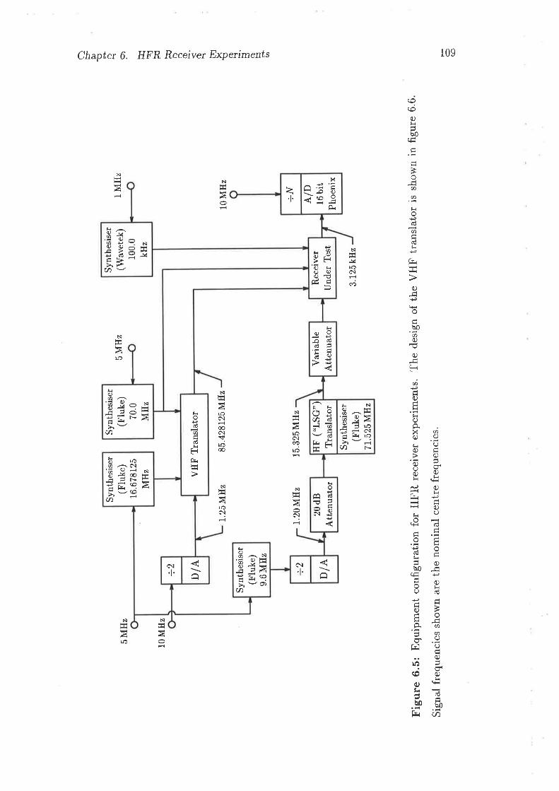
+N A/D
16 b
irP
hoen
ix
Syn
thes
iser
(Wav
etek
)10
0.0
kHz
Rec
eive
rU
nder
Tes
tV
aria
ble
Atte
nuat
or
Syn
thes
iser
(FIu
ke)
70.0
MIIz
HF
("LS
G")
TÌan
slat
orS
ynth
esis
er(F
luke
)7l
.525
MH
z
VH
F Tr
ansl
ator
Syn
thes
iser
(Flu
ke)
16.6
7812
5M
Hz
20 d
BA
ttenu
ator
:9 D/A., DIL
Syn
thes
iser
(Flu
ke)
9.6
MH
z
85.4
2812
5 M
Hz
15.3
25 M
Hz
1.25
MH
z
1.20
MH
z
5 M
Hz
l MH
z5
MH
z
10 M
Hz
10M
Hz
3.12
5 kH
z
Figu
re 6
.5: E
quip
men
t co
nfig
urat
ion
for H
FR re
ceiv
er e
xper
imen
ts. T
he d
esig
n of
the
VH
F tra
nsla
tor
is s
how
n in
figu
re 6
.6
Sig
nal f
requ
enci
es s
how
n ar
e th
e no
min
al c
entre
freq
uenc
ies.
o Þ + o Þ ts¿i t:q Þo o o o I t! X -c o tst o (n O C.o
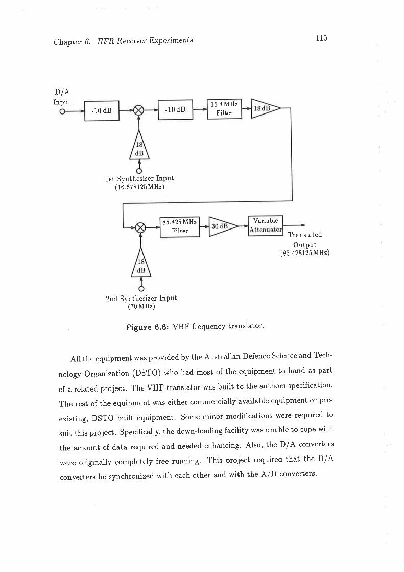
Chapter 6. HFR Receiver Experiments
Dl¡^Input
110
1st Synthesiser InPut(16.678125MH2)
TranslatedOutput
(85.428125 MHz)
2nd Synthesizer InPut(70MHz)
Figure 6.6: VHF frequency translator'
All the equipment was provided by the Australian Defence science and Tech-
nology Organization (DSTO) who had most of the equipment to hand as part
of a related project. The VHF translator was built to the authors specification'
The rest of the equipment was either commercially available equipment or pre-
existing, DSTO built equipment. some minor modifications Ïvere required to
suit this project. specifically, the down-loading facility was unable to cope with
the amount of data required and needed enhancing. Also, the D/A converters
were originally completely free running. This project required that the D/A
converters be synchronized with each other and with the A/D converters'
15.4 MHzFilter-10 dB-10 dB
tVariable85.425 MHz
Filter
Chapter 6. HFR Receiver Experiments 111
6.3.2 Test Signals
The choice of test signals is not entirely straight forward. More traditional
methods of measuring distortion employing sinusoids have the advantage that
it is relatively easy to isolate the nonlinear response because it is at a different
frequency than the linear response. However, section 3.7 points out that a broad
band signal is required to completely identify a general nonlinearity. Also, the
optimum estimation of a system depends on the probability density function
of the input signal (section 3.5), so it is desirable for the test signals to have
a similar probability density function to the signals applied to the receiver in
normal operation. The normal receiver input can be considered as a sum of the
backscatter from an infinite sum of infinitesimal backscatterers. Howevet, these
components are not'independent processes because the illuminating signal is
strongly correlated and the central limit theorem is not strictly applicable. If
the probability density function of the test signal is not exactly the same as
the normal receiver input, an estimation will still be achieved, but it will be
sub-optimal.
Band limited quasi-Gaussian pseudo-random noise was selected for these
receiver experiments. The author does not claim that this signal is in any
sense ideal, but its properties are a reasonable approximation to the properties
mentioned in the last paragraph. The quasi-Gaussian distribution was achieved
by summing 10 uniformly distributed random variables. The local oscillator
signal was chosen to be a band limited FMCW ("chirp") signal with sweep
rates and repetition rates typical of normal operation.
Both the FMCW and pseudo-random noise signals were band limited by
Fourier transforming, zeroing frequencies outside the desired band and inverse
transforming3. Doing this digitally allows the specification for the analogue
sSince the signal is generated by cycling through the set of samples, it is truly periodic
and hence this method of bandpass filtering is exact'
Chapter 6. HFR Receivet ExPeilments I12
filters in the frequency translators (figure 6.5) to be relaxed'
6.3.3 Chirp Generation by Phase Accumulation
Experience has shown that generating sinusoids on a general purpose computer
is best done by incrementing the phase modulo 2zr. If the obvious formula is
used r(ú) : sin(øú) for ú = 0,t1,t2,...tn, then there is considerable phase noise
if /,, is large. That is because, even with double precision arithmetic, the error in
c¿ú for large ú is a signifrcant proportion of 2z-. Consequently, the best algorithm
1. Initialize S and A'$.
2. r(t): cos(/).
3. Set ó*Ó+LÓ
4. lf.ó )zrset Ó*Ó-2r.
5. Repeat from step 2
This algorithm reduces phase noise by keeping lÓl S ".
A similar algorithm can be used for a linear frequency sweep. First note
that the instantaneous frequency can be defined by
r=L\. (6.1)2¡r dt'
and a linear sweep can be defined
/(¿) :/o+(fi - f")*: ,fo * Ut - fo)f*,ú.
(6.2)
(6.3)
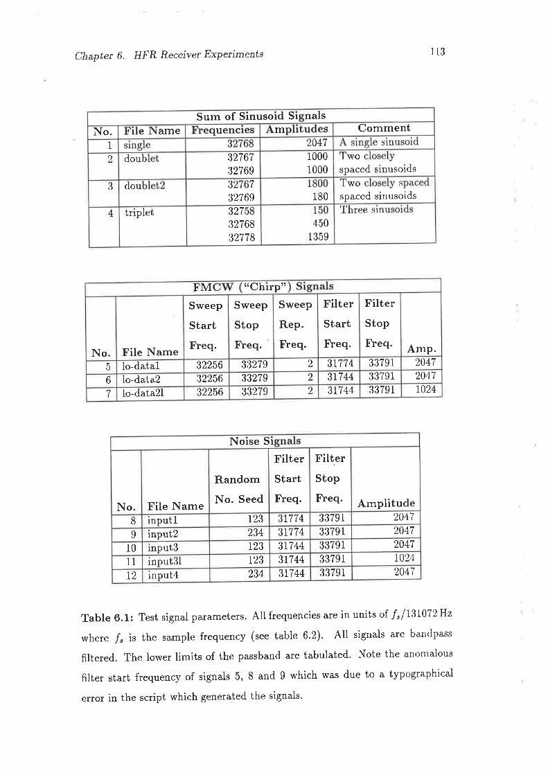
Sum of Sinus nalss IolCommentt smuameI eNo.
sln20471
spaced sinusoidsTwo1000
10003276932762 doub
Twospaced sinusoids
S1
1 8032 I
32769dou3
Three s1n1
4501359
3273276832778
triplet4
Chapter 6, HFR Receiver ExPeilments 113
Table 6.1: Test signal parameters. All frequencies are in units of f "lI3L072Hzwhere /" is the sample frequency (see table 6.2). All signals are bandpass
filtered. The lower limits of the passband are tabulated. Note the anomalous
filter start frequency of signals 5, 8 and 9 which was due to a typographical
error in the script which generated the signals'
FM ,,Chirptt
Amp.
FilterStop
Freq.
Sweep
ReP.
FYeq.
FilterStartFreq.
Sweep
Stop
FYeq.
Sweep
StartFreq.
No. File Name33791 20472 3177433279322565 lo-data1
20473t744 3379133279 232256lo-data26r024337912 3r7443327932256I lo-data2l
N SiolseFilterStop
Freq. Amplitude
FilterStartFreq.
RandomNo. Seed
No. File Name204737774 33791t23inputl820473379131774234I input2
33791 20473r74412310 input3t024337913r744r2311 input3l20473r744 33791234input412
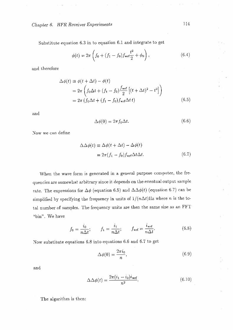
Chapter 6. HFR Receiver Experiments
and therefore
Ad(¿) =ó(t+aú) -ö(t)
Substitute equation 6.3 in to equation 6.1 and integrate to get
ó(t):r. (r,+ (/, - rùr*nÇ* t,) ,
Lt4
(6.4)
:2r:2tr (fs\t + (lt - /o)/*"rA¿ ú) (6.5)
and
Ad(0) :2îfs\t. (6.6)
Now we can define
AAd(¿) : LÓ(t+ ar) - LÓ(t)
:2r(h - /o)/*,rA¿Aú. (6.7)
When the wave form is generated in a general purpose computer, the fre-
quencies are somewhat arbitrary since it depends on the eventual output sample
rate. The expressions for A/ (equation 6.5) and AAd(ú) (equation 6.7) can be
simplified by specifying the frequency in units of. I l@Lt)Hz where n is the to-
tal number of samples. The frequency units are then the same size as an FFT((bin". We have
(r,o, + (/, - rù+[{t + rt)' -,'])
"ioIo : -;i. 2t n ?wrl.f _ ...................._. t .
- _Jr-n\,t, J*"-nAú
Now substitute equations 6.8 into equations 6'6 and 6'7 to get
Ad(o) :+,and
ir - io)i*"r
(6.8)
(6 e)
The algorithm is then:
aad(¿) : 2nn2
(6.10)
Chapter 6. HFR Receiver Experiments i15
1. Initialize ó, Lö and AA/.
2. r(n): cos(/).
3. Set Ó*Ó+Ad
4. If.ó )zrset Ó*Ó-2tc.
5. Set Ló * Ad + AAd
6. Repeat from steP 2
It is not normally necessary to ensure that lA/l ( zr since that would correspond
to a maximum frequency above the Nyquist sampling rate'
6.3.4 Sampling Rates
The sample rates and frequencies have been chosen so the data contains an
integer number of cycles. This allows manipulations to be done by Fast Fourier
Transforms (FFT's) and Inverse Fast Fourier Transforms (IFFT's) without win-
dowing (or with a rectangular window).
The problem of aliases of the desired signal has already been mentioned in
section 6.3.1, However, with careful choice of sampling rates the requirements
of the translator filters can be relaxed further. The presence of aliases results
in energy centred at frequencies
f, : nf "" ! h, (6'11)
f¿ - mf ", L fz,, (6'12)
for the input (r) and local oscillator (/) signals. If these two signals are trans-
lated and mixed (inside the receiver) the resultant signal has components cen-
tred at frequencies
f :rf,,*mf",+å+ fz*k, (6.13)
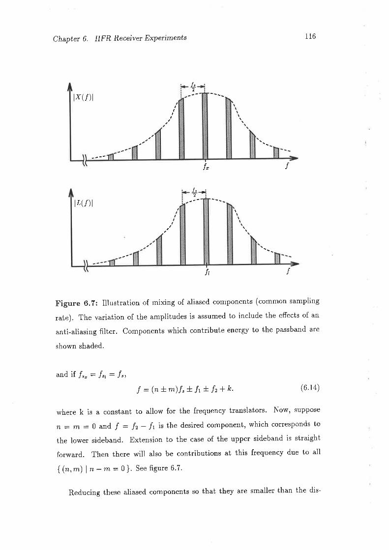
Chapter 6. HFR Receiver Experiments
tx(/)ltI
116
(6.14)
,
rJ'2
t,
t"2
+!
f
t¿(/)lI
ft r
Figure 6.7: Illustration of mixing of aliased components (common sampling
rate). The variation of the amplitudes is assumed to include the effects of an
anti-aliasing filter. Components which contribute energy to the passband are
shown shaded.
andif f"":f",:f",f :(nt*)f,tå+ lz-lk.
where k is a constant to allow for the frequency translators' Now, suppose
n : rn: 0 and f : r, - ,f, ir the desired component, which corresponds to
the lower sideband. Extension to the case of the upper sideband is straight
forward. Then there will also be contributions at this frequency due to all
{(",*) I , - *: 0 }. See figure 6'7.
Reducing these aliased components so that they are smaller than the dis-
Chapter 6. HFR Receiver Expetiments 1.r7
tortion components is difficult. The design target for these experiments was to
be able to detect nonlinear distortion components 80 dB down from the linear
components (based on two tone IMD measurements). At a sampling frequency
of SMHz and assuming the signal is at a centre frequency of f '14: l.2\MHz,
the requirement for the anti-aliasing filter is 80 dB rejection 2.5MHz from the
centre frequency at a centre frequency of 15 MHz. The passband needs to be
approximately 100 kHz wide. This is a fall off of some 47 dB per decade which
is certainly possible, but becomes more difficult to meet if there are also con-
straints on passband ripple and phase linearity'
Now suppose the sampling rates are different and /"" : f ", - 2Al where
a/ is the band width of the signal. Referring to figure 6'8, the aliases of
desired components do not have commensurate frequencies except at a distant
frequency such that
mÍ,,12: (rn + I)f ""12: (nn + 1)(/", 12 - Ll),
+
+
Í", 1m:1ñ1 -"
A,r,= (*-t)r,,P, (6.15)
where afi is the distance from the centre frequency. using the previous num-
bers of SMHz for /", and 100kHz for A/' A/t :60MHz' This figure is greater
than the centre frequency of 15 MHz and filtering of components this far from
the centre frequency must be done by a filter on the D/A output, before the
translation process. In practice, a post translation frlter is still desirable because
the band limited components illustrated in figures 6.7 and 6'8 become broad-
ened by any distortion encountered before the receiver first mixer' However, if
the first aliased components are reduced by 20 dB, then the 3rd and higher or-
der distortion components are reduced by 60 dB or greater so if the anti-aliasing
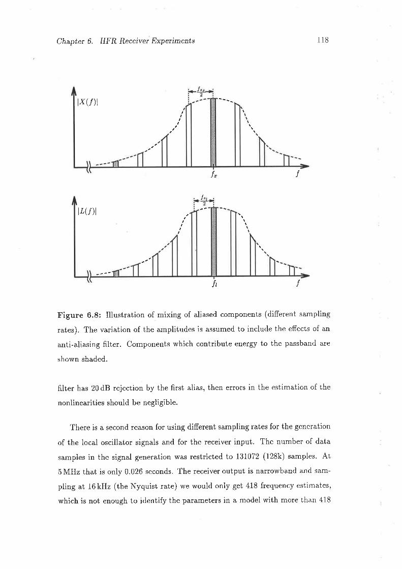
Chapter 6. HFR Receiver Experiments
lx(/)l
118
,
r, f
ÍlL(f)l
,tI
t
lt r
Figure 6.8: Illustration of mixing of aliased components (different sampling
rates). The variation of the amplitudes is assumed to include the effects of an
anti-aliasing filter. Components which contribute energy to the passband are
shown shaded.
filter has 20 dB rejection by the first alias, then errors in the estimation of the
nonlinearities should be negligible.
There is a second reason for using different sampling rates for the generation
of the local oscillator signals and for the receiver input. The number of data
samples in the signal generation was restricted to 731072 (128k) samples. At
5 MHz that is only 0.026 seconds. The receiver output is narrowband and sam-
pling at 16 kHz (the Nyquist rate) we would only get 418 frequency estimates,
which is not enough to identify the parameters in a model with more than 418
Chapter 6. HFR Receiver Experiments 119
parameters even assuming zero noise. 'Ihere is a mismatch in the quantity of
information supplied in the input and the quantity of information in the output.
A total of 256k data samples (taking into account the input signal and the local
oscillator signal) have been input, but we have only got 418 independent sam-
ples out. The reason, of course, is that most of the information has been filtered
out by the receivers frequency selectivity. By sampling the local oscillator data
and the input data at slightiy different rates, the combined sequence does not
repeat until many cycles through the input data.
Because the input sequences are repeated, the spectra of the signals are in
the form of a fine comb. The repetition rate of the RF input sequence, and
hence the line spacing of the comb, is
f- - 4'8 x 10⁶ : 86.62109 J75HzJra - 2tz55 x26 ,:+(f xs) nz, (6.16)
and
- 5.0 x 10⁶f --- :38.1469726563H2rrt - 2t755 x 26 t-,:l(r,) u,. (6.17)
The repetition rate of the combined input is the largest common factor of. f,,and /", which is
(5f,o: h:1.52587890625H2. (6.18)
Note that the spacing of the lines in the output spectrum (equation 6.i8) is
very much finer than the spacing of the lines in the input spectrum (equation
6.16). Thus there is much more information (by u factor of.24) in the output
spectrum than there would be if the local oscillator input and the RF input
spectrum had a constant sampling rate of 4.8 MHz.
To simplify FFT processing, the output sampling rate should be a power
of two multiple of h.. A/D sampling rates are derived by dividing a 10 MHz
Chapter 6. HFR Receivet Expetiments 120
clock, so the output sampling rate staisfies
f""107
n
and
T"o: rflfro, (6.1e)
which implies
Tnn :218 x 52. (6'20)
If m :211, then from equation 6.18, f"o:56 :3l25nz' Since rn must be
a po\Mer of two, higher sampling rates must also be power of two multiples of
3I25Hz which is easier to picture. The other requirement on the A/D sampling
rate is that it must satisfy the Nyquist rate for the output data.
In practice, components of the receiver output wele present outside the
nominal passbanda and a higher sampling rate was used than would otherwise
be expected. The actual sampling rates used are tabulated in table 6'2'
Port Rate No. PeriodLO InputRF InputOutput
5.0 MHz4.8 MHz
25kIJz
r3r072t3t072131072
0.02620.0273
5.24
Table 6.2: SamPling Parameters
6.4 Analysis Algorithms
6.4.L Complex Envelope Processing
whilst figures 6.2, 6.3 and 6.4 in principle show methods of estimating and
correcting distortion in a receiver, the data rates at the inputs are much higher
aThis was an experimental receiver and the filter determining the band width differed
considerably from that actually used in the Radar'
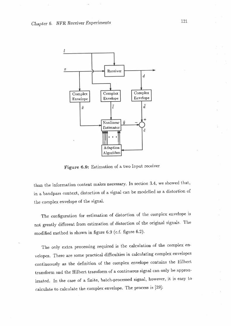
Chapter 6. HFR Receivet Experiments l2r
Figure 6.9: Estimation of a two Input receiver
than the information content makes necessary. In section 3'4, we showed that,
in a bandpass context, distortion of a signal can be modelled as a distortion of
the complex envelope of the signal'
The configuration for estimation of distortion of the complex envelope is
not greatly difierent from estimation of distortion of the original signals' The
modified method is shown in figure 6'9 (c'f' figure 6'2)'
The only extra processing required is the calculation of the complex en-
velopes. There are some practical difficulties in calculating complex envelopes
continuously as the definition of the complex envelope contains the Hilbert
transform and the Hilbert t¡ansform of a continuous signal can only be approx-
imated. In the case of a finite, batch-processed signal, however, it is easy to
calculate to calculate the complex envelope. The process is [29]:
rd
d
+
e
Receiver
ComplexEnvelope
ComplexEnvelope
ComplexEnvelope
NonlinearEstimator
AdaptionAlgorithm
Chapter 6. HFR Receiver Experiments 122
1. Take the Fourier Transform X(ø) : f @(t))
2. Zero the negative frequencies
3. Shift (ø) down by ro .
4. Inverse Fourier Transform
Operation 3, above, is slightly complicated by the way the output of an FFT is
stored in an arrays.
6.4.2 The Ideal Receiver and Sample Interpolation
Figures 6.3 and 6.2 both have an "Ideal Receiver" in the block diagram. The
HFR receiver performs two functions, one is the frequency translation function
and the other is the "de-ramping" function. Doing these operations directly
involves emulating the mixing and filtering processes in the real receiver (see
figure 6,1) which is complex and numerically intensive6. It is much easier to
emulate an ideal receiver by performing operations on the complex envelopes of
the RF input and local oscillator signals. Essentially, the complex envelope of
the ideal receiver output is simply the product of the complex envelopes of the
RF and LO inputs. There are, in practice, two complications'
The receiver de-ramping process (the first mixer of figure fig-rx-block), in-
volves mixing and selecting the lower sideband. Assuming the original signals
wer: real, Y(ro - ø) : Y(ro * c,.,)*, where y(ú) is the output of the first mixer
prior to filtering. Therefore, the de-ramping can be modelled by swapping the
positive and negative frequency components of Í.(r) prior to the multiplication
with the local oscillator signal. This reversing of frequency components can be
sPositive frequencies first, then negative frequenctes.
oAlthough simplifications can be made by reducing the number of conversions if ideal
filtering operations are performed.
Chapter 6. HFR Receiver Experiments t23
performed by taking the Fourier transform, doing the swapping, and taking the
inverse Fourier transform, but it is more efficient to combine it as part of the
process of finding the complex envelope. This modified complex envelope ã¡(l)
can be found thus (c.f. section 6.4.1):
1. Take the Fourier Transform X(r) : F (r(t))
2. Zero the positiue frequencies
3. Shift X(r) up by us'
4. Inverse Fourier Transform.
The second complication in calculating the output of the ideal receiver, is
due to the different sampling rates for the RF and LO inputs (see table 6.2).
We need to interpolate to a common higher sampling rate. Further, since both
inputs have the same number of samples but different sampling rates, both
signals need to be replicated so they have a common duration. The lowest
common multiple of the sample rates is 25f", - 241"t - l2}MHz as can be
seen from equations 6.16 and 6.17 and table 6.2. Interpolation in the time
domain is the same as zero padding in the frequency domain so the straight
forward method is (for the RF input):
l. Replicate to a length of 24 x 128k
2. Take the FFT
3. Pad with zeros to a length of 25 x 24 x 128k.
4. Take the Inverse FFT.
The same process is used for the LO signal except using 25 instead of 24 and
visa-versa. The problem with this approach is that it requires a 78643200 sample
IFFT which is quite impractical.
Chapter 6. HFR Receiver ExPeúments t24
A more effi,cient method was derived taking advantage of the fact that the
input signals are band limited and the receiver output is band limited. For the
purpose of comparison with the sampled receiver output, 128k samples is the
maximum. In fact, because the receiver sampling rate is high enough to allow
a guard band, we need less than 128k samples. The strategy is to perform the
simulation in such a way as to minimize the number of samples to be stored
at any point. one way of achieving this is to work with a complex envelope
representation as early as possible. Another useful property is that replication
in the time domain is equivalent to zero stufÊng7 in the frequency domain' The
entire process (including calculation of the complex envelopes) is as follows (see
also figure 6.10):
1. Take FFT's of the RF(ø) and LO(/) inputs'
2. Zero the positiue frequencies of x(r) and the negatiae frequencies of L(ø)'
3. Shift X(r) downby cd6 and L(u) up by'o'
4. stuff x(r) with (24 - 1) zeros between each sample, and L(ø) with (25
- 1) zeros between each sample. Note that because X(r) and L(ø) are
narrowband this step can be preformed without increasing the number of
samples. This step is equivalent to replication in the time domain'
5. zeropad x(ø) and L(ø). In principle v/e zero pad to 24x25 x 128k, but in
practice, the tails of all zeros can be ignored. That is because the next two
steps are equivalent to convolution in the frequency domain, and a long
tail of zeros wider tLan the band width of the signal doesn't contribute
to the convolution. In practice we zetopad to the smallest power of two
greater than the sum of the band widths of x(cu) and L(o).
6. Take the IFFTs of õ(ú) : F-rx(u) and ilt¡ : F-rL(u)'
Tlnserting zero samples between the existing samples
Chapter 6. HFR Receiver Experiments t25
7. Output õ¡(ú) and ilt¡ *tti.tr are the complex envelopes of ø(ú) and /(ú)
converted to a common sampling rate.
8. Multiply ñít) ana i(t) and output as the complex envelope of the output
of an ideal receiver
The measured output data must also be converted to a complex envelope at
the same interpolated sampling rate. The interpolation (by zero padding in the
frequency domain) is performed in the same way as for the RF and LO inputs.
The sampling interval includes 8 repetitionss of the output data therefore, only
1 in 8 frequency estimates will be non zero. In practice noise and spurious
signals mean this is not strictly true, however, setting them to zero effectively
improves the signal to noise ratio of the sampled output. Once this has been
done, there is little point in maintaining such a high frequency resolution and
the zero samples can be removed in a process which is the inverse to the zero
stuffing performed for the processing of the RF and LO data.
6.4.3 Adaptive filter Algorithms
The direct solution method of estimating the filter weights was used because it
is simple, robust and has no convergence time. Since the nonlinear distortion
was assumed to be of small energy compared to the linear components, the
eigenvalue spread would be large and gradient algorithms would probably not
converge sufficiently in a reasonable time to estimate the nonlinear weights.
Unfortunately, the computation time for the direct solution method is excessive
for a large number of taps which prompted the author to investigate the RLS
methods (section D). The RLS methods have not been successfully implemented
in software and this is a suggested topic for further research.
8In practice most results were obtained by discarding the first samples to avoid the startup
transient. In those cases only 64k samples rvere processed and the relevant factor here was 4.
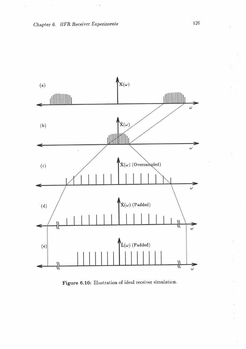
Chapter 6. HFR Receiver Expetiments
ar)
u)
c..') (Padded)
a,) (Padded)
126
(b)
(")
(") )
(t
u
(t
a
(d)
a
(")
u)(
Figure 6.10: Illustration of ideal receiver simulation'
Chapter 6. HFR Receiver Experiments r27
The direct solution method provides the best possible estimation of the
weights for a given number of input samples. To that extent it places an upper
bound on the performance achievable by any other methods.
Two versions of the program were written, one using the QR algorithm to
solve the Wiener-Hopf equations and one using singular value decomposition
(SVD). Whilst the auto-correlation matrix is guaranteed to be positive semi-
definite, it is not necessarily positive definite. The QR algorithm is well behaved
with poorly conditioned matrices, but if the correlation matrix is singular, a
unique solution does not exist. In the linear case, it is known [+Z] that a singular
correlation matrix results when the power spectrum is zero at some frequency'
The input to the adaptive filter is, in the HFR experiments, band limited. In the
estimation case, the input occupies almost the full band width but the number
of frequency estimates was rounded up to a power of two when the complex
envelopes were calculated and consequently the signal does not occupy the full
band width. In the correction case, the band width is even narrower as it has
been reduced by the receiver selectivity. If a single input corrector is used, this
can be alleviated by reducing the effective sample rate of both the input and
the desired output, but in the case of a two input corrector we are stuck with
a narrowband width input. One solution is to add random noise to ensure that
the spectrum never goes to zero. Another, possibly more elegant, method is to
use singular value decomposition (SVD).
The SVD process returns the matrices { U, y, ^ I A : (J*-t
^y-1 } and
consequently the solution of the Wiener-Hopf equation 5'21 is
c:v{r-7(J*a. (6.21)
The matrix z\ is a diagonal matrix of eigenvalues l; in reducing order. Inverting
 is performed simply by inverting each of the elements. The trick is to say
that if any of the À; ate zeto (or less than a certain value) then replace lf À;
with zero. In equation 6.21, zeroing some of the À; corresponds to zeroing the
corresponding columns of U and the corresponding rows of. V. Zeroing some
Chapter 6. HFR Receiver Expeilments t28
of the elements of A-1 reduces the norm of vector c. This method can be
summarized as detecting when a system is under determined and selecting the
soiution which has a minimum norm'
6.5 Results
6.5.1 Equipment and Procedure Verification
In order to gain confidence in both the hardware and the software some simple
test signals were used initially. with signal 4 of table 6'1 as the RF input and
signal 3 of table 6.1 as the Lo input, the spectrum of the measured output is
shown in figure 6.11. The strange looking noise floor was found to be due to
the receiver start up transient. omitting the first lk samples from the analysis
results in the spectrum in figure 6.12. The spectrum of the simulated output of
an ideai receiver with the same inputs is shown in figure 6'13'
Observe that the simulated output of an ideal receiver (figure 6.13) correctly
estimates the main output components of the real receiver (figure 6'12)' This
case is also simple enough to be able to predict how the simulated output
should look. Figure 6.13, ciearly shows a doublet shifted by each of the three
sinusoids in the triplet. observe in figure 6.12 the 3rd harmonic distortion
clustered around 10 kHz and the rather larger odd order distortion components
clustered around 0 Hz. Also observe a small amount of IMD distortion products
observable as "sidebands" of the "ideai" signal. The shifted doublets of flgure
6.13 appear to have been converted to shifted triplets in figure 6'12' This
is attributable to the local oscillator input being overdriven to the point of
clippinge.
eThis is the normal operating mode for such a mixer
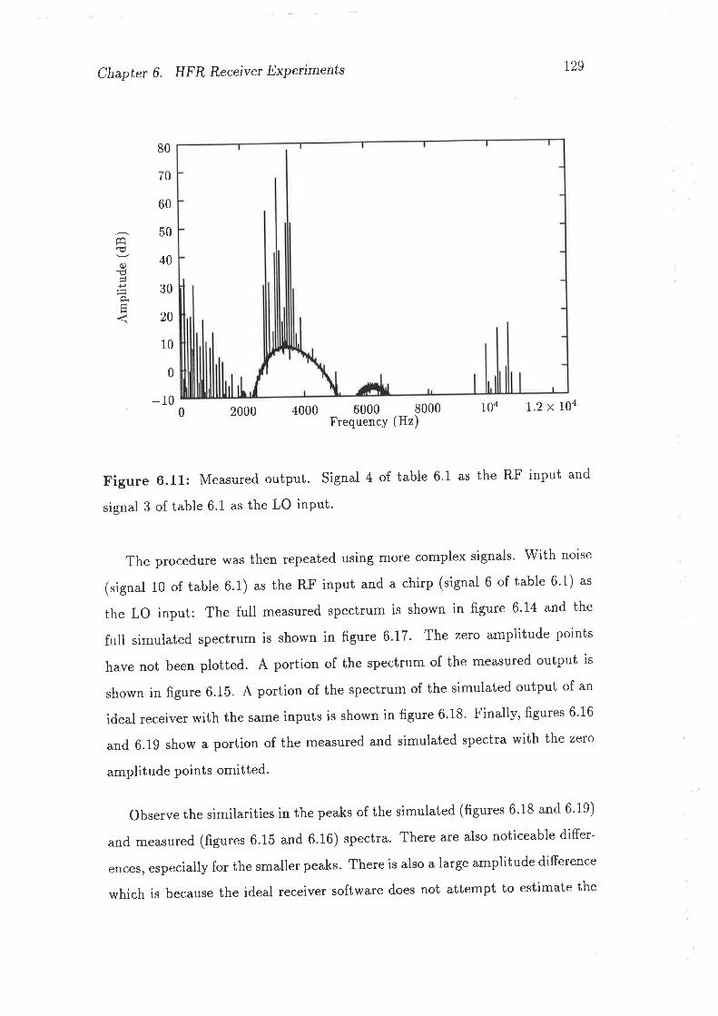
Chapter 6. HFR Receiver Expetiments t29
80
70
60
50
40
30
20
10
0
-10 6000 8000Frequency (Hz)
104 1.2 x L040 2000 4000
Figure 6.11: Measured output. signal 4 of table 6.1 as the RF input and
signal 3 of table 6.1 as the LO input'
The procedure was then repeated using more complex signals. with norse
(signal 10 of table 6.1) as the RF input and a chirp (signal 6 of table 6.1) as
the LO input: The full measured spectrum is shown in figure 6'14 and the
full simulated spectrum is shown in figure 6.17' The zero amplitude points
have not been plotted. A portion of the spectrum of the measured output is
shown in figure 6.15. A portion of the spectrum of the simulated output of an
ideal receiver with the same inputs is shown in figure 6.18. Finally, figures 6.16
and 6.19 show a portion of the measured and simulated spectra with the zero
amplitude points omitted.
observe the similarities in the peaks of the simulated (figures 6.18 and 6.19)
and measured (figures 6.15 and 6.16) spectra. There are also noticeable differ-
ences, especially for the smaller peaks. There is also a large amplitude difference
which is because the ideal receiver software does not attempt to estimate the
Êq€c)
€È
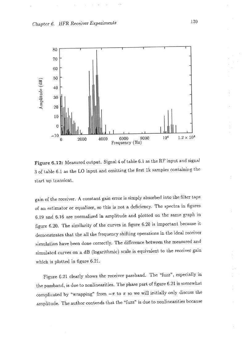
Chapter 6. HFR Receiver Experiments
80
70
60
50
40
30
20
10
0
-10
ÊqEC)€È
130
104 r.2 x ro40 2000 4000
Figure 6.12: Measured output. signal4 of table 6.1 as the RF input and signal
3 of table 6.1 as the Lo input and omitting the first lk samples containing the
start up transient.
gain of the receiver. A constant gain error is simply absorbed into the filter taps
of an estimator or equalizer, so this is not a deficiency. The spectra in figures
6.19 and 6.16 are normalized in amplitude and plotted on the same graph in
figure 6.20. The similarity of the curves in figure 6.20 is important because it
demonstrates that the all the frequency shifting operations in the ideal receiver
simulation have been done correctly. The difference between the measured and
simulated curves on a dB (logarithmic) scale is equivalent to the receiver gain
which is plotted in figure 6.21.
Figure 6.21 clearly shows the receiver passband. The "f171Z2", especially in
the passband, is due to nonlinearities. 'l'he phase part of figure 6'21 is somewhat
complicated by "wrapping" from -zr to n so we will initially only discuss the
amplitude. The author contends that the "r:uzz" is due to nonlinearities because
6000 8000Frequency (Hz)
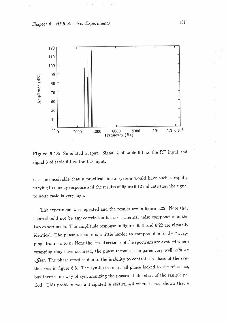
Chaptet 6. HFR Receiver Experiments
t20
110
100
90
80
70
60
50
40
30
ÊaÉq)€
À
131
104 1.2 x r}a0 2000 4000
Figure 6.13: simulated output. signal 4 of table 6.1 as the RF input and
signal 3 of table 6.1 as the LO input.
it is inconceivable that a practical linear system would have such a rapidly
varying frequency response and the results offigure 6.12 indicate that the signal
to noise ratio is verY high.
The experiment was repeated and the results are in figure 6'22' Note that
there should not be any correlation between thermal noise components in the
two experiments. The amplitude response in figures 6.21 and 6'22 are virtually
identical. The phase response is a little harder to compare due to the "wrap-
ping" from -zr to zr. None the less, if sections of the spectrum are avoided where
wrapping may have occurred, the phase response compales very well with an
offset. The phase offset is due to the inability to control the phase of the syn-
thesizers in figure 6.5. The synthesizers are all phase locked to the reference,
but there is no way of synchronizing the phases at the start of the sample pe-
riod. This problem tffas anticipated in section 4.4 where it was shown that a
6000 8000Frequency (Hz)
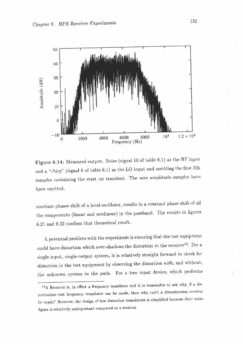
Chapter 6. HFR Receiver Expetiments r32
104 1.2 x 10⁴
Êa€q)€
50
40
30
20
10
0
-100 2000 4000
Figure 6.14: Measured output. Noise (signal 10 of table 6'1) as the RF input
and a "chirp" (signal 6 of table 6.1) as the LO input and omitting the first 32k
samples containing the start up transient
been omitted.
The zero amPlitude samPles have
constant phases shift of a local oscillator, results in a constant phase shift of all
the components (linear and nonlinear) in the passband. The results in figures
6.21 and 6.22 confirm that theoretical result'
A potential problem with the experiment is ensuring that the test equipment
could have distortion which over-shadows the distortion in the receiverlO' For a
single input, single output system, it is relatively straight forward to check for
distortion in the test equipment by observing the distortion with, and without'
the unknown system in the path. For a two input device, which performs
104 Receiver is, in efiect a frequency translator and it is reasonable to ask why, if a dis-
tortionless test frequency translator can be made, then why can't a distortionless tecerver
be made? However, the design of low distortion translators is simplified because their noise
figure is relatively unimportant compared to a receiver'
6000 8000Frequency (Hz)
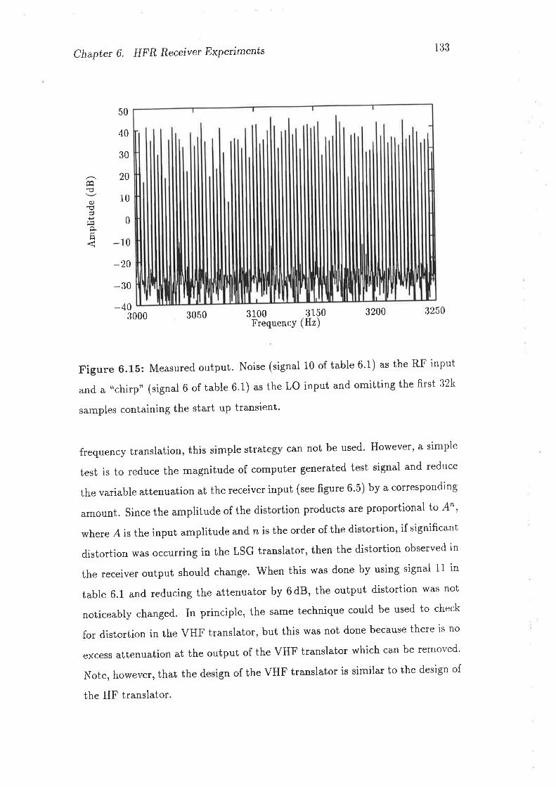
Chapter 6. HFR Receivet Expefiments i33
50
40
30
20
10
0
-10
-20
-30
-40 3100 3150Frequency (Hz)
3200 32503000 3050
Figure 6.15: Measured. output. Noise (signal 10 of table 6.1) as the RF input
and a "chirp" (signal 6 of table 6.1) as the LO input and omitting the first 32k
samples containing the start up transient'
frequency translation, this simple strategy can not be used. However, a simple
test is to reduce the magnitude of computer generated test signal and reduce
the variable attenuation at the receiver input (see figure 6.5) by a corresponding
amount. since the amplitude of the distortion products are proportion al to A" ,
where A is the input amplitude and n is the order of the distortion, if significant
distortion was occurring in the LsG translator, then the distortion observed in
the receiver output should change. When this was done by using signal l1 in
table 6.1 and reducing the attenuator by 6dB, the output distortion was not
noticeably changed. In principle, the same technique could be used to check
for distortion in the vHF translator, but this was not done because there is no
excess attenuation at the output of the vHF translator which can be removed'
Note, however, that the design of the vHF translator is similar to the design of
É€o)Éa€ÈÀ
the HF translator
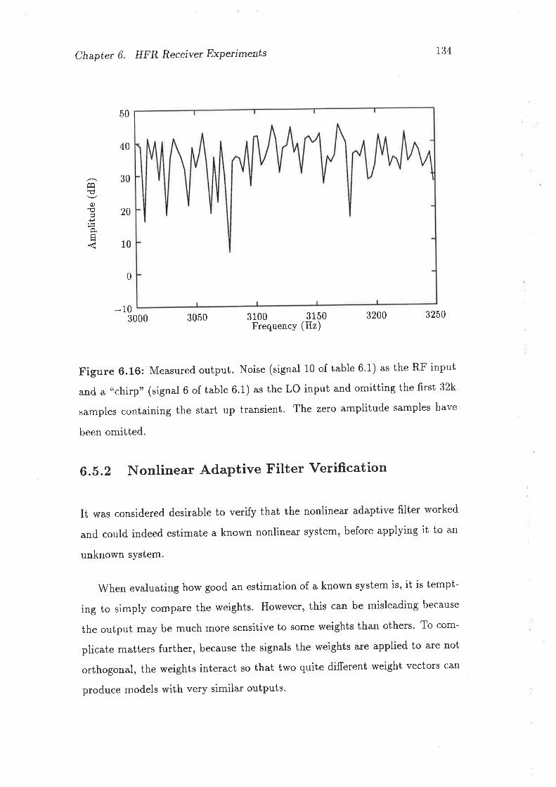
Chapter 6. HFR Receiver Expeilments 134
50
30
10
-10 3200 32503000 3050
Figure 6.16: Measured output. Noise (signal 10 of table 6.1) as the RF input
and a ,,chirp', (signal 6 of table 6.1) as the LO input and omitting the first 32k
samples containing the start up transient. The zero amplitude samples have
been omitted.
6.5.2 Nonlinear Adaptive Filter Verification
It was considered desirable to verify that the nonlinear adaptive filter worked
and could indeed estimate a known nonlinear system, before applying it to an
unknown system.
when evaluating how good an estimation of a known system is, it is tempt-
ing to simply compare the weights. However, this can be misleading because
the output may be much more sensitive to some weights than others' To com-
plicate matters further, because the signals the weights are applied to are not
orthogonal, the weights interact so that two quite different weight vectors can
produce models with very similar outputs.
40
20
Êq
q)
H
0
3100 3150Frequency (Hz)
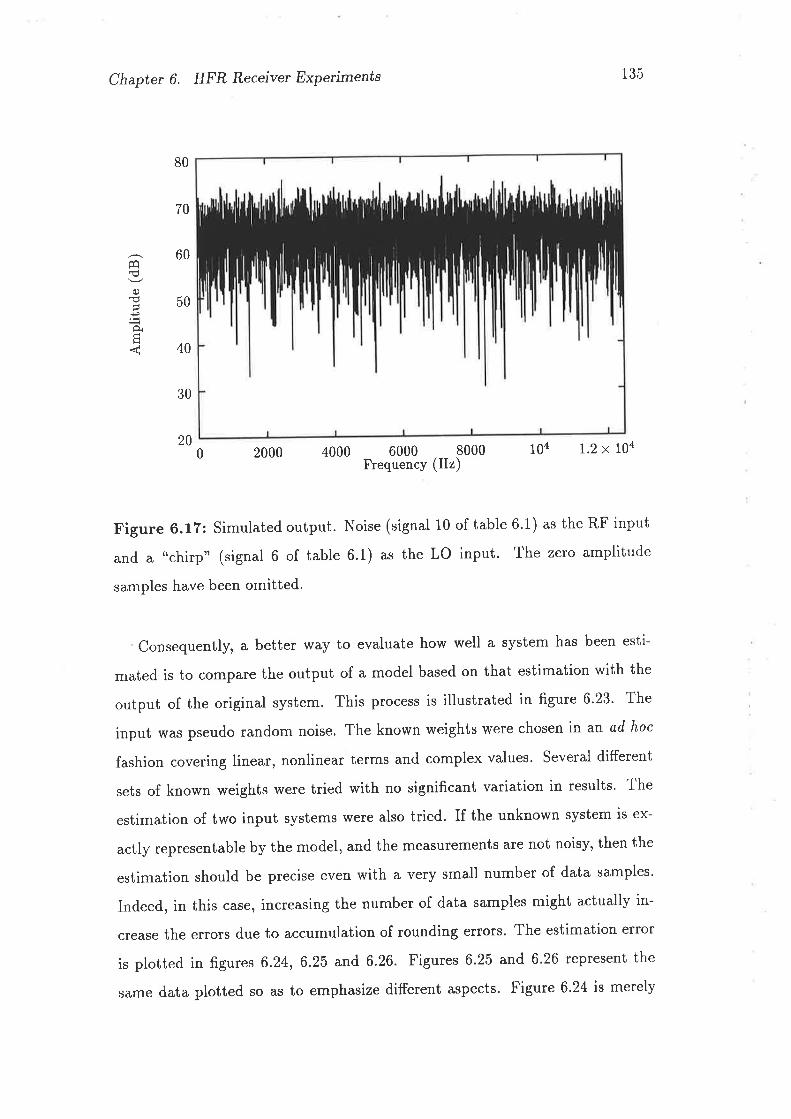
Chapter 6. HFR Receivet ExpeÅments 135
104 1.2 x roa
Êq
0.)d
ÈH
80
70
60
50
40
30
200 2000 4000
Figure 6.17: Simulated output. Noise (signal 10 of table 6.1) as the RF input
and a ,,chirp" (signal 6 of table 6.1) as the LO input. The zero amplitrrde
samples have been omitted.
consequently, a better way to evaluate how well a system has been esti-
mated is to compare the output of a model based on that estimation with the
output of the original system. This process is illustrated in figure 6'23' The
input was pseudo random noise, The known weights were chosen in an ad hoc
fashion covering linear, nonlinear terms and complex values. Several different
sets of known weights were tried with no significant variation in results. The
estimation of two input systems were also tried. If the unknown system is ex-
actly representable by the model, and the measurements are not noisy, then the
estimation should be precise even with a very small number of data samples'
Indeed, in this case, increasing the number of data samples might actually in-
crease the errors due to accumulation of rounding errors. The estimation error
is plotted in figures 6.24, 6.25 and 6.26. Figures 6.25 and 6'26 represent the
same data plotted so as to emphasize different aspects. Figure 6'24 is merely
6000 8000Frequency (Hz)
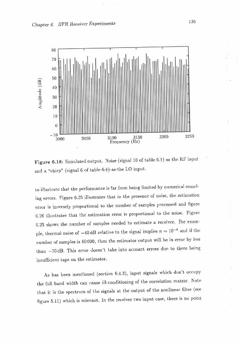
Chapter 6. HFR Receiver Expetiments
80
70
60
50
40
30
20
10
0
-10
ÊaÉo
È
136
3200 32503000 3050 3100 3150
FrequencY (Hz)
Figure 6.18: simulated output. Noise (signal 10 of table 6'1) as the RF input
and a "chirp" (signal 6 of table 6J) as the LO input'
to illustrate that the performance is far from being limited by numerical round-
ing errors. Figure 6.25 illustrates that in the presence of noise, the estimation
error is inversely proportional to the number of samples processed and figure
6.26 illustrates that the estimation error is proportional to the noise' Figure
6.25 shows the number of samples needed to estimate a receiver' For exam-
ple, thermal noise of -40 dB relaiive to the signal implies n : I}-a and if the
number of samples is 60 000, then the estimator output will be in error by less
than -70 dB. This error d.oesn't take into account errors due to there being
insufñcient taps on the estimator'
As has been mentioned (section 6.4.3), input signals which don't occupy
the futl band width can cause ill-conditioning of the correlation matrix' Note
that it is the spectrum of the signals at the output of the nonlinear filter (see
figure 5.11) which is relevant. In the receiver two input case, there is no point
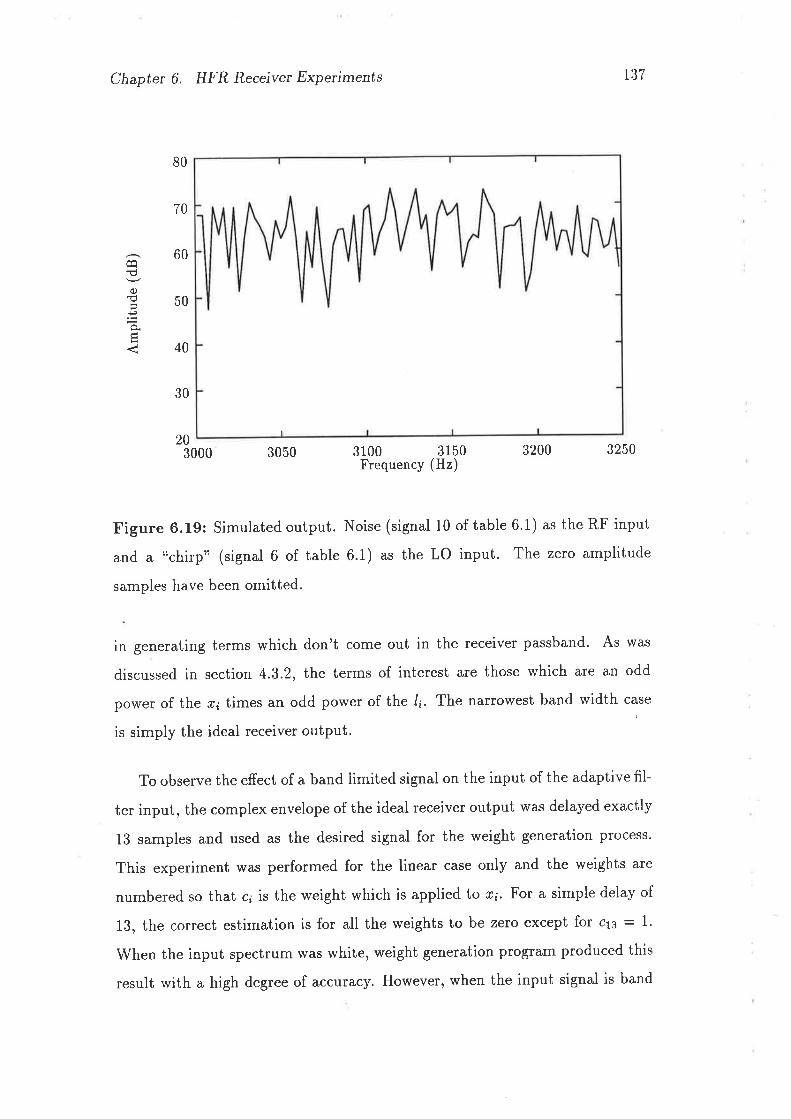
Chapter 6. HFR Receiver Experiments 137
3000 3050 3200 3250
Figure 6.19: Simulated output. Noise (signal 10 of table 6.1) as the RF input
and a "chirp" (signal 6 of table 6.1) as the LO input. The zero amplitude
samples have been omitted.
in generating terms which don't come out in the receiver passband. As was
discussed in section 4.3.2, the terms of interest are those which are an odd
power of the r¡ times an odd power of the /¡. The narrowest band width case
is simply the ideal receiver output.
To observe the effect of a band limited signal on the input of the adaptive fil-
ter input, the complex envelope of the ideal receiver output was delayed exactly
13 samples and used as the desired signal for the weight generation process.
This experiment was performed for the linear case only and the weights are
numbered so that c¡ is the weight which is applied to x;' For a simple delay of
13, the correct estimation is for all the weights to be zero except for c13 : 1'
When the input spectrum was white, weight generation program produced this
result with a high degree of accuracy. However, when the input signal is band
Fq
0)d
80
70
60
50
40
30
20 3100 3150Frequency (Hz)
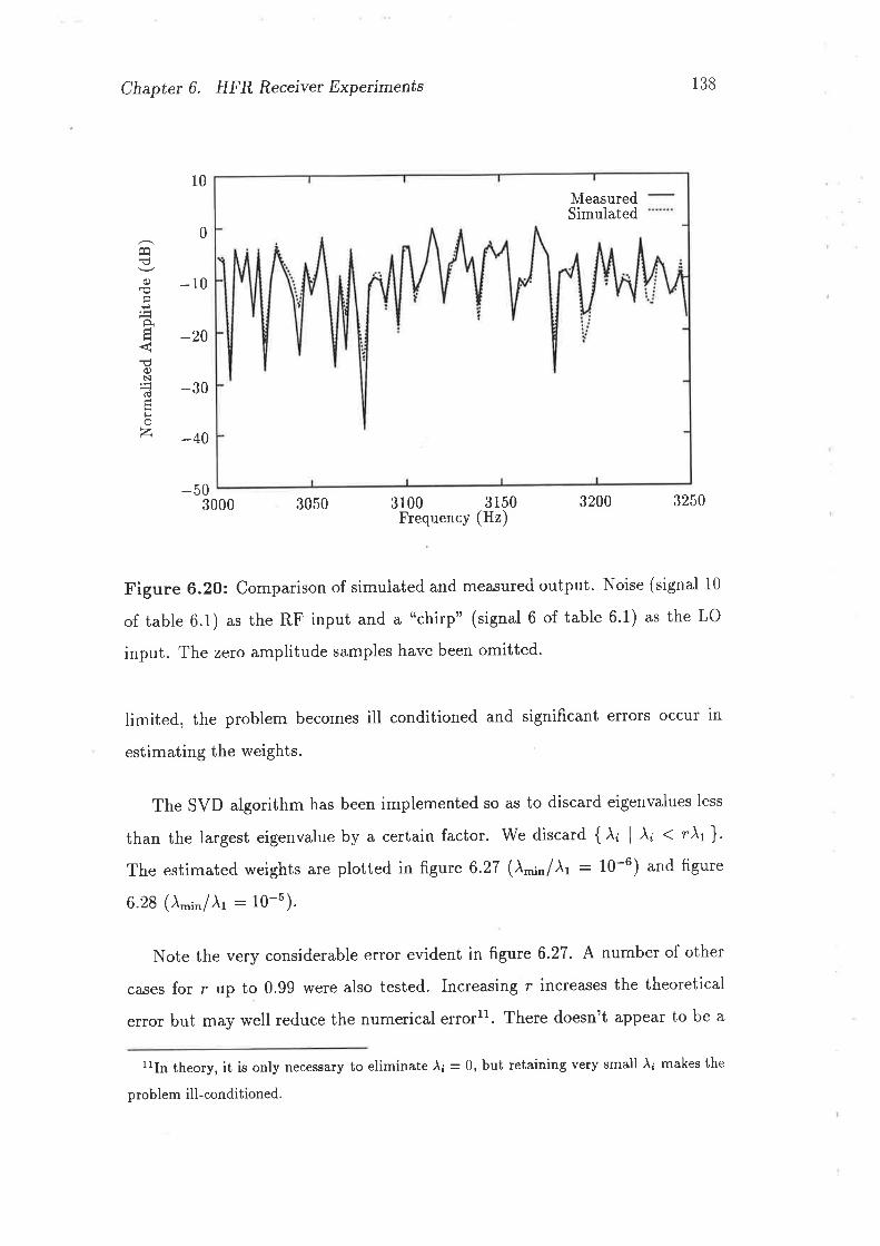
Chapter 6. HFR Receiver Expeúments 138
10
-10
-20
-40
-50 3200 32503000 3050
Figure 6.20: Comparison of simulated and measured output. Noise (signal 10
of table 6.1) as the RF input and a "chirp" (signal 6 of table 6.1) as the LO
input. The zero amplitude samples have been omitted.
limited, the problem becomes ill conditioned and significant errors occur ln
estimating the weights.
The SVD algorithm has been implemented so as to discard eigenvalues less
than the largest eigenvalue by a certain factor. We discard { Àt I À¿ < tÀt }.
The estimated weights are plotted in figure 6.27 (1,ú^ l\, : 10-6) and figure
6.28 (À",i./À1 : 10-5).
Note the very considerable error evident in figure 6.27. A number of other
cases for r up to 0.99 were also tested. Increasing r increases the theoretical
error but may well reduce the numerical errorll. There doesn't appear to be a
1lln theory, it is only necessary to eliminate À¡ = 0, but retaining very small À¡ makes the
problem ill-conditioned.
0
-30
Êa
c)
Ê
Ec)Nd
troz
3100 3150Frequency (Hz)
MeasuredSimulated
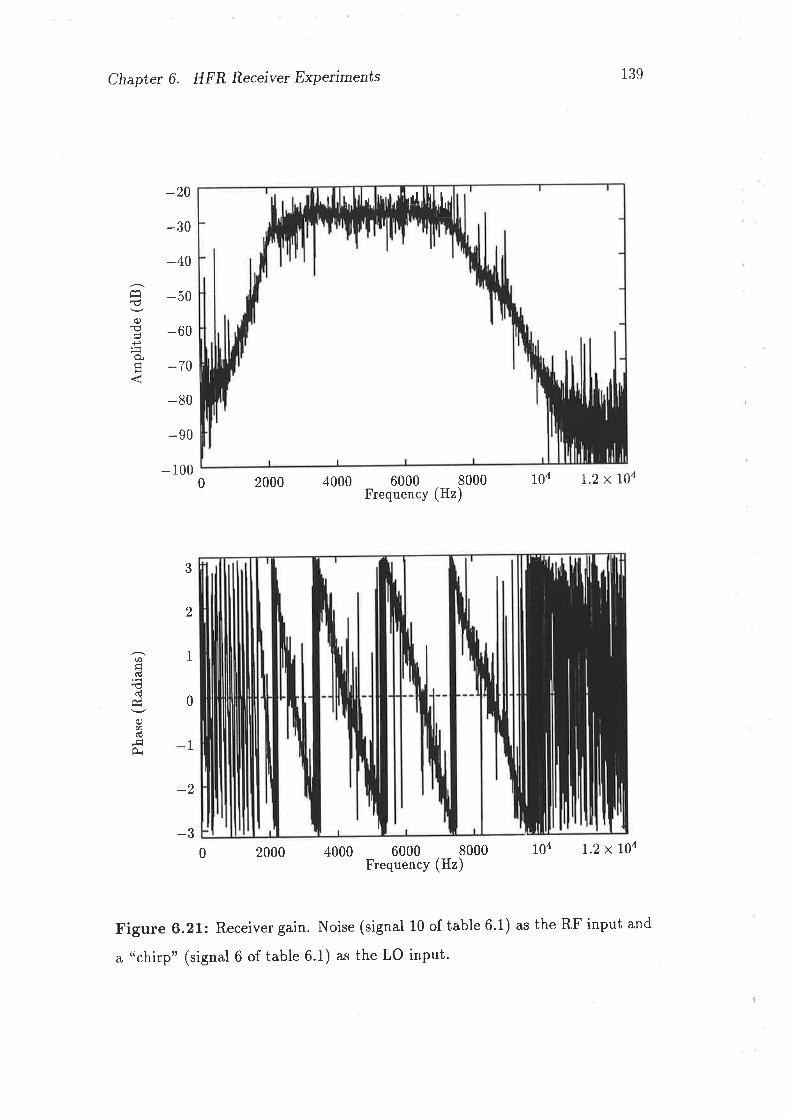
Chapter 6. HFR Receiver Experiments
-20
-30
-40
-50
-60
-70
-80
-90
- 1000 2000 4000
1
-2
-3
Êq€G)
À
139
r04 7.2 x r1a
104 1.2 x 10⁴
6000 8000Frequency (Hz)
3
2
1
0
Ø
ddØd
0 2000 4000
Figure 6,212 Receiver gain. Noise (signal 10 of table 6'1) as the RF input and
a "chirp" (signal 6 of table 6.1) as the LO input.
6000 8000Frequency (Hz)
¡,L rd¡. tu
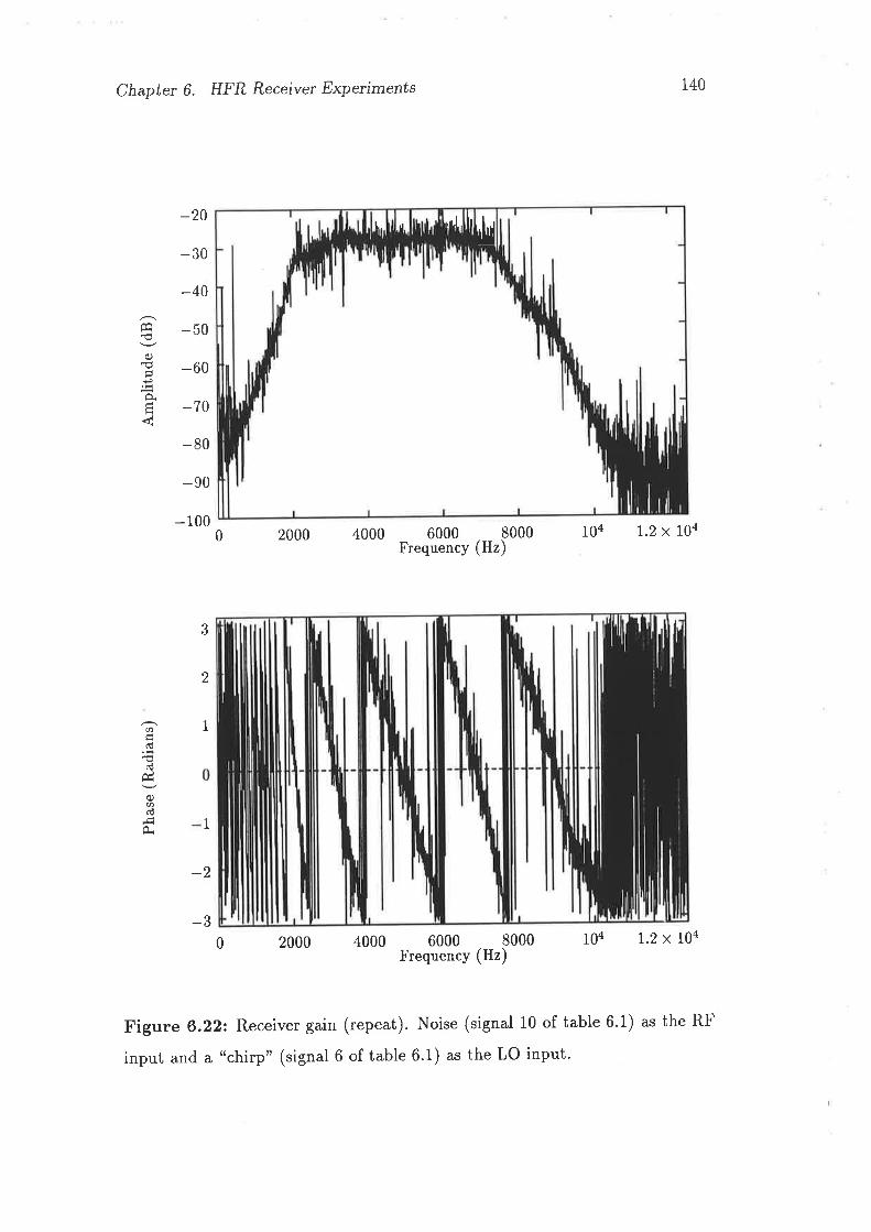
Chapter 6. HFR Receiver Experiments
-20
-30
-40
-50
-60
-70
-80
-90
- 1000 2000 4000
1
-2
-3
Êq
o)
ÈH
140
104 1.2 x l}a
lo4 1.2 x 1oa
6000 8000Frequency (Hz)
3
2
1Ø
ddùq)Ørd
Êi
0 2000 4000
Figure 6.22 Receiver gain (repeat). Noise (signal 10 of table 6.1) as the RF
input and a "chirp" (signal 6 of table 6'1) as the LO input'
6000 8000Frequency (Hz)
h'r.lt. ¡. ùr
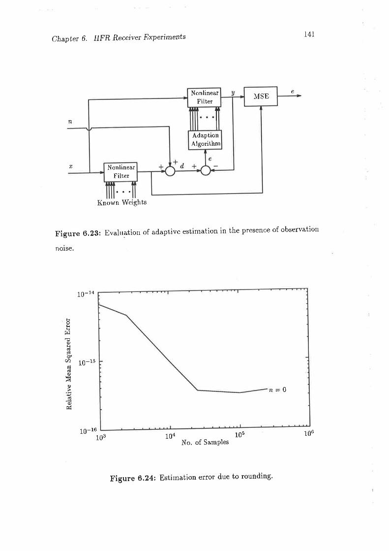
Chapter 6. HFR Receiver Expetiments T4T
106
e
n
Í
norse.
Known Weights
Figure 6.23: Evaluation of adaptive estimation in the presence of observation
ßilrli
14
q)Êrd
U)
d0)àq)
do
l¿t
10-14
10-15
10-161 g3 104 105
No. of Samples
MSENonlinearFilter
AdaptionAlgorithm
+NonlinearFilter
0n
Figure 6,242 Estimation error due to rounding'
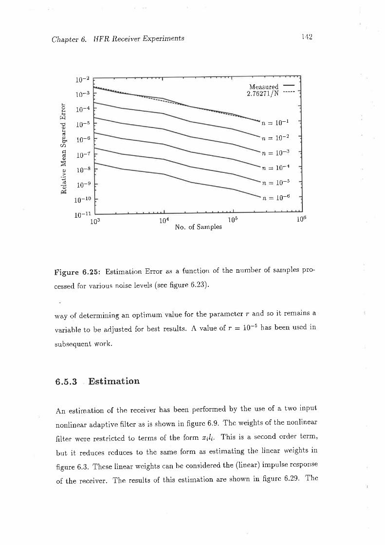
Chapter 6. HFR Receiver Experiments
l0-2
10-3
10-4
10-5
10-6
10-7
10-8
10-e
10-10
10-11
r42
ÈkÈfrlE
CJÈd
(hHd0)
À0)
d0)Å
103 104 105 106No. of Samples
Figure 6,262 Estimation Error as a function of the number of samples pro-
cessed. for various noise levels (see figure 6.23)'
way of determining an optimum value for the parameter r and so it remains a
variable to be adjusted for best results. A value of r : 10-5 has been used in
subsequent work.
6.5.3 Estimation
An estimation of the receiver has been performed by the use of a two input
nonlinear adaptive filter as is shown in figure 6.9. The weights of the nonlinear
filter were restricted to terms of the form r;/;' This is a second order term,
but it reduces reduces to the same form as estimating the linear weights in
figure 6.3. These linear weights can be considered the (linear) impulse response
of the receiver. The results of this estimation are shown in figure 6'29' The
n = 10-r
n = 10-2
n = 10-3
n = I}-an = 10-5
n: 10-6
vleasureo2.7627r1N ----'
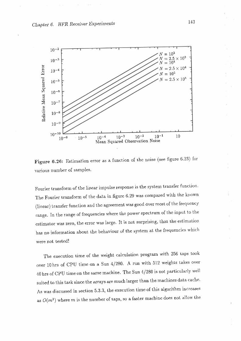
Chaptet 6. HFR Receivet Expeñments
10-2
10-3
10-4
10-5
10-6
10-7
10-8
10-e
10-10
143
ÈÈlir¡o)È(€
(nHd0)à0)
(€o)
10-6 10-5 10
Figure 6.26: Estimation error as a function of the noise (see figure 6'23) for
various number of samPles
Fourier transform of the linear impulse response is the system transfer function'
The Fourier transform of the data in figure 6.29 was compared with the known
(linear) transfer function and the agreement was good Óver most of the frequency
range. In the range of frequencies where the power spectrum of the input to the
estimator was zero, the error was large. It is not surprising, that the estimation
has no information about the behaviour of the system at the frequencies which
were not tested!
The execution time of the weight calculation program with 256 taps took
over 10hrs of cPu time on a sun 41280. A run with 512 weights takes over
40 hrs of CpU time on the same machine. The Sun 4 1280 is not particularly well
suited to this task since the arrays are much larger than the machines data cache'
As was discussed in section 5.3.3, the execution time of this algorithm increases
as o(m2) where rn is the number of taps, so a faster machine does not allow the
10-4 10-3 10-2 __ 10-ttvtã.tt Squared Observation Noise
y'Í = 103N=2.5x10³N=104l{=2.5x10⁴N-105y'{=2.5x10⁵
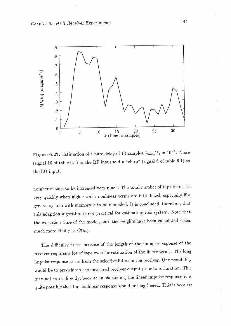
Chapter 6. HFR Receiver Experiments
5 10 25 30
Figure 6,27t Estimation of a pure delay of 13 samples, À,,¡,,/Àr : 10-6' Noise
(signal 10 of table 6.1) as the RF input and a "chirp" (signal 6 of table 6.1) as
the LO input.
number of taps to be increased very much. The total number of taps increases
very quickly when higher order nonlinear terms are introduced, especially if a
general system with memory is to be modelled. It is concluded, therefore, that
this adaption algorithm is not practical for estimating this system' Note that
the execution time of the model, once the weights have been calculated scales
much more kindly as O(nz).
The difÊculty arises because of the length of the impulse response of the
receiver requires a lot of taps even for estimation of the linear terms' The long
impulse response arises from the selective filters in the receiver' one possìbility
would be to pre-whiten the measured receiver output prior to estimation' This
may not work directly, because in shortening the linear impulse response it is
quite possible that the nonlinear response would be lengthened. This is because
r44
Éã
{J
bod!
.¡è
-s¿
.9
.8
.7
.6
.5
,4
.3
.2
1
00 15 20
k (time in samples)
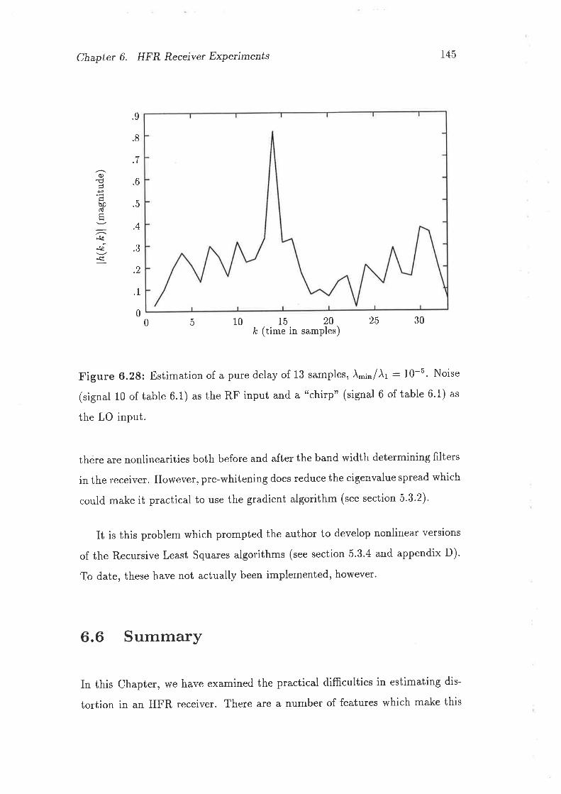
Chapter 6. HFR Receiver Experiments
5 10
r45
q)
Hbo
H
-Jê-s¿
.9
.8
.7
.6
.b
,4
.3
.2
.1
00 15 20
,t (time in samples)25 30
Figure 6.28: Estimation of a pure delay of 13 samples, À"¡,/À1 : 10-5. Noise
(signal 10 of table 6.1) as the RF input and a "chirp" (signal 6 of table 6'1) as
the LO input.
thére are nonlinearities both before and after the band width determining filters
in the receiver. However, pre-whitening does reduce the eigenvalue spread which
could make it practical to use the gradient algorithm (see section 5.3'2)'
It is this problem which prompted the author to develop nonlinear versions
of the Recursive Least Squares algorithms (see section 5.3.4 and appendix D).
To date, these have not actually been implemented, however'
6.6 Summary
In this Chapter, we have examined the practical difficulties in estimating dis-
tortion in an HFR receiver. There are a number of features which make this
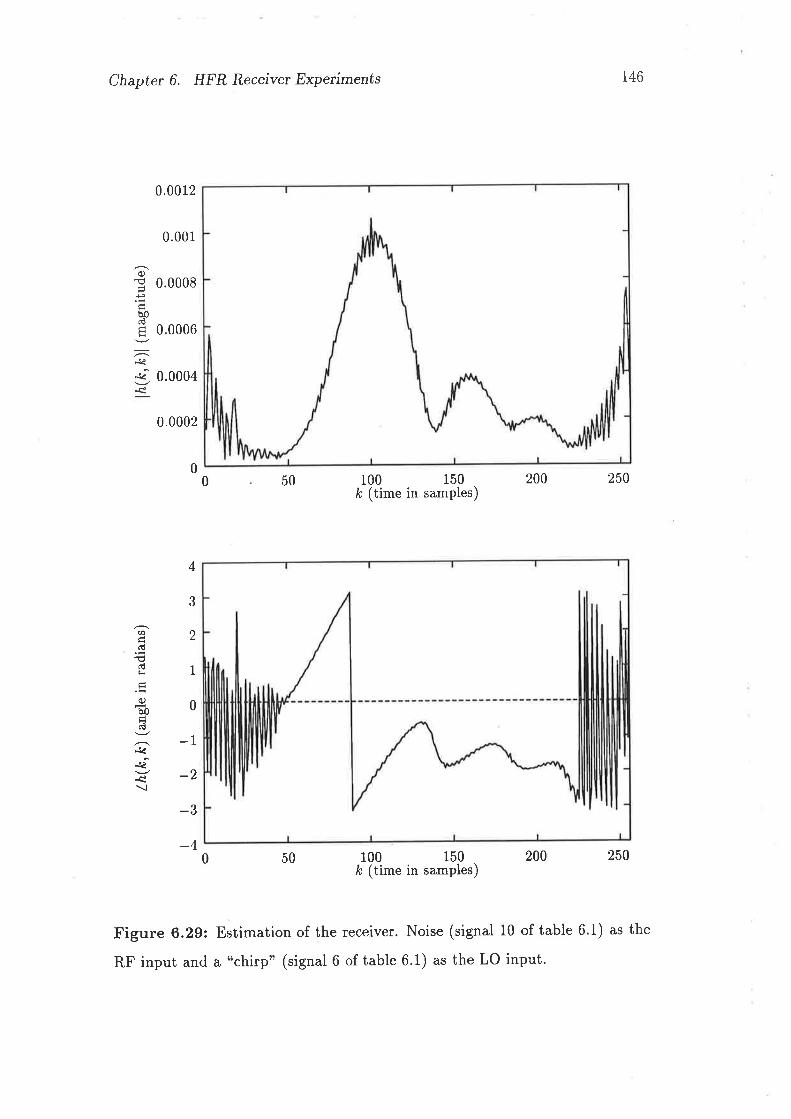
Chapter 6. HFR Receiver Expetiments
0.0012
0.001
0.0002
146
.0008
.0006
004
0
0
0.0
0)
HbodH
-¡l.sê
00 50 100 150
k (time in samples)
100 150,t (time in samples)
200 250
(A
d€dÈq)bod
.S¿
-sè
\
4
3
2
1
0
-1
-2
-3
-40 200 250
Figure 6.292 Estimation of the receiver. Noise (signal 10 of table 6.1) as the
RF input and a "chirp" (signal 6 of table 6.1) as the LO input.
50
Chapter 6. HFR Receivet Expetiments
experiment difierent to other experiments which have been described in the
literature. SpecificallY
1. The receiver must be modelled as a two input device. The phase of the
Iocal oscillator input, relative to the RF input, can not be measured or
controlledl2.
2. The receiver has slight, but important, nonlinear distortion in the pres-
ence of large linear distortion. The linear distortion is inherent in the high
frequency selectivity of the receiver and implies a long impulse response.
The small power of the nonlinear components relative to the linear com-
ponents implies a large eigenvalue spread. The linear weights must be
calculated accurately if the nonlinear distortion is to be seen.
3. The receiver's inputs and outputs are at different frequencies' This was
dealt with by estimating the distortion in the complex envelope instead
of estìmating the distortion of the original signals'
4. The band width of the signals applied to the receiver's inputs should be
very much greater than the band width of the receiver output to ad-
equately probe the front end circuitry. consequently, it is difficult to
provide enough input samples so that enough information is available in
the output for the estimation to be done'
Item 2 above has not been completely solved. The only algorithm imple-
mented to date (direct solution of the wiener-Hopf equations), has sufficient
accuracy, but has excessive computation time' Gradient algorithms, are fast
enough in terms of operations per step, but take too long to convelge to a point
where the small nonlinear distortion can be estimated. It may be possible to re-
duce the eigenvalue spread by pre-whitening. Nonlinear recursive least squares
algorithms have been derived but not implemented to date. It is possible that
t47
l2All bhe signals are phase locked, but there is no way to set the initial phase
Chapter 6. HFR Receiver Experiments 148
other difficulties, such as stability in the face of rounding errors' might be a
problem with the RLS algorithms. Finding a suitable adaption algorithm is a
topic for future research.
Item 4, above, can be handled by sampling the input data at slightly different
sampling rates. This complicates the processing of the data considerably, but
the problem is tractable.
Experimental evidence has been gained for the theoretical resuit derived in
section 4.4 where it was shown that a constant phase shift of a local oscillator,
results in a constant phase shift of ali the components (linear and nonlinear) in
the passband (see item 1 above)'
Chapter 7
Conclusron
One of the factors limiting the performance of many systems is nonlinear dis-
tortion. Traditional ways of correcting distortion such as feedback and feedfor-
ward have limitations for broad band high-frequency systems, especially sys-
tems which include frequency translators. Pre-distortion or post-distortion is
an alternative way of reducing over all distortion which is useful in many cir-
cumstances where feedback or feedforward is impractical or impossible. One of
the more demanding applications is High Frequency Radar (HFR) Receivers.
In this thesis a number of theoretical and practical problems relevant to mod-
elling and correcting nonlinear distortion in HFR Receivers have been solved.
Designing a pre-distortion or post-distortion to preform nonlinear correction
is equivalent to finding a model of the nonlinear inverse, thus modelling and
correction are very similar processes. It is desirable to know whether a model
is sufflciently general to model the system' or' in the case of a corrector, the
system inverse.
In chapter 2, signal dependent ways of characterizing distortion were ex-
amined. "Harmonic Distortion", "Intelmodulation Distortion", "Cross Mod-
ulation Distortion" and "Polyspectra" were discussed. These terms refer to
measures of distortion rather than models of distortion'
149
Chapter 7. Concluston150
It is possible (though not simple) to use these measures of distortion to
evaluate the parameters of a model although, as we saw in chapter 3, a general
model can not be evaluated with simple inputs consisting of only a few sinusoids'
In chapter 3, various parametric characterizations of distortion were consid-
ered to frnd one suitable for estimating or correcting bandpass systems' The
distortion in systems modelled by power series, amplitude and phase describing
functions and volterra series was analyzed for the case of bandpass inputs and
outputs. In these cases it was shown that distortion in a bandpass context can
be considered as distortion of the complex envelope of the signal' This property
is of significance for bandpass systems since it means that much less data need
be processed to estimate ot correct a nonlinear system. The wiener model of
non-linearities has also been derived but consideration of the bandpass case was
deferred to chaPter 4.
The power series model is a special case of the amplitude and phase describ-
ing function model. Both the power series model and the amplitude and phase
describing function model are special cases of the volterra series model and the
form of the Volterra kernels has been deduced'
From consideration of the frequency domain lepresentation of the volterra
kernels it was shown that, for band limited inputs, the Volterra kernels of the
model and of the actual system need only match for ar within a hyper-cube of
interest. This is analogous to requiring the model of a linear system to match
the actual transfer function over a frequency range of interest'
It was shown that for a sufficiently narrowband input signal, any distorting
system describable by a Volterra series could be approximated by the amplitude
and phase describing function model' It was also shown that testing with a sin-
gle sinusoid, even at a number of difierent frequencies, is inadequate to check
whether amplitude and phase describing functions are an adequate model or
whether a more general Volterra series model is necessary' Frequency indepen-
Chapter 7. Conclusion 151
dence of the amplitude and phase describing functions, as measured by a single
sinusoid is a necessary, but not sufÊcient condition for the amplitude and phase
describing function model to be applicable.
Many bandpass systems, including HFR Receivers, perform frequency trans-
lation functions. This is done by "mixing" with one or more local oscillator
signals. Thus, such systems are actually multiple input systems. In chapter
4 it was observed that mixer manufacturers' linearity specifications implicitly
assume a rather simple model of distortion in a two input device. This assump-
tion has been critically examined and found to be invalid if the mixer does not
have a "pure"1 sinusoidal local oscillator'
Most mixer applications employ a sinusoidal local oscillator but some mod-
ern mixer appiications use non-sinusoidal local oscillator signals such as a linear
frequency sweep (a "chirp") and caution must be exercised in applying per-
formance measurements made with a sinusoidal local oscillator to these ap-
plications. It may be that a "chirp" changed frequency slowly enough to be
considered a sinusoid, but this would depend on the mixer and the frequency
sweep rate. The author speculates that useful relationships might arise from
studying the case of constant envelope signals as local oscillators'
It was shown that in the case of a bandpass system, a change in phase of
one of the input signals results in the same change in phase of all components of
the output signal within the passband. This result is of practical importance in
the modelling of distortion in a receiver where it is impossible or impracticable
to measure the local oscillator signals. It was also shown, by example, that this
is not the case for broad band systems'
The discrete time volterra series is attractive to model or correct nonlinear
rA distorted sinusoid is satisfactory since the distortion can be considered part of the
block N" in figure figure 4,1. A "broadened" sinusoid (perhaps due to amplitude or phase
modulation) is not satisfactorY.
Chapter 7. Conclusion r52
distortion, since it is capable of approximating a very large class of nonlinear
functionals arbitrarily well. In chapter 5, it was seen how the discrete time
Volterra series can form the basis for a nonlinear digital filter. Nonlinear filters
can be made to adapt to a required characteristic. The nonlinear adaptive filter
can be used in the roles of estimators, predictors and equalizers in the same
way as linear adaptive filters.
The LMS gradient algorithm and the method of directly soiving the Wiener-
Hopf equations used in linear adaptive filters are directly applicable to the
nonlinear case. Other more efÊcient linear adaption algorithms such as the
Recursive Least Squares algorithms are not directly applicable to the nonlinear
case. The Recursive Least Squares algorithm has been extended to the nonlinear
case in section 5.3.4 and appendix D. The LMS gradient algorithm and the
RLS algorithm require O(nm) operations, whereas the Direct Solution of the
Wiener-Hopf equations requires O(nm2) operations assuming that the weights
are updated infrequently so that number of operations is dominated by the
calculation of the correlation matrix A. The RLS algorithms and direct solution
of the Wiener-Hopf equations have zero convergence time'
The single input nonlinear digital filter is simply extendible to two or more
inputs. The adaption algorithms can also be extended to the multi-input case.
The implementation of a suite of programs for efficiently implementing and
testing multi-input nonlinear adaptive filters has been discussed.
In Chapter 6, we examined in detail the practical difficulties in estimating
distortion in an HFR receiver. There are a number of features which make this
experiment different to other experiments which have been described in the
literature. SpecificallY:
1. The receiver must be modelled as a two input device. The phase of the
local oscillator input, relative to the RF input, can not be measured or
Chapter 7. Conclusrcn 153
controlled2.
2. The receiver has slight, but important, nonlinear distortion in the pres-
ence of large linear distortion. The linear distortion is inherent in the high
frequency selectivity of the receiver and implies a long impulse response.
The small po\ryer of the nonlinear components relative to the linear com-
ponents implies a large eigenvalue spread. The linear weights must be
calculated accurately if the nonlinear distortion is to be seen.
3. The receiver's inputs and outputs are at different frequencies. This was
dealt with by estimating the distortion in the complex envelope instead
of estimating the distortion of the original signals.
4. The band width of the signals applied to the receiver's inputs should be
very much greater than the band width of the receiver output to ade-
quately probe the front end circuitry. Consequently it is difÊcult to pro-
vide enough input samples so that enough information is available in the
output for the estimation to be done'
Item 4, above, can be handled by sampling the input data at slightly different
sampling rates. This complicates the processing of the data considerably, but
the problem is tractable.
Experimental evidence has been gained for the theoretical result derived in
section 4.4 where it was shown that a constant phase shift of a local oscillator,
results in a constant phase shift of all the components (linear and nonlinear) in
the passband (see item 1 above).
Item 2, above, places severe constraints on the adaption algorithms and
prompted the development of the RLS algorithms. However, the only algo-
rithm implemented to date (direct solution of the Wiener-Hopf equations), has
sufficient accuracy, but has excessive computation time.
2All the signals are phase locked, but there is no way to set the initial phase'
Chapter 7. Conclusrcn
There are a number of areas requiring further investigatlon.
Avenues for further theoretical work are as follows:
o The equivalence of distortion of a signal and distortion of its complex
envelope needs to be extended to the two input case. We have assumed
this equivalence in the experimental work.
o There may be useful insights to be gained looking at distortion in two
input systems where one input is constant envelope. The work done in
chapter 4 with sinusoidai oscillators is a special case.
There is plenty of scope for improvement in algorithms for nonlinear adaptive
filters. Gradient algorithms, are fast enough in terms of operations per step,
but take too long to converge to a point where the small nonlinear distortion
can be estimated. It may be possible to reduce the eigenvalue spread by pre-
whitening. Nonlinear recursive least squares algorithms have been derived in
this thesis, but not implemented to date. Issues such as stability in the face
of rounding errors need to be addressed and it may be possible to derive more
eficient versions.
Because of the inefficiency of the algorithms available, the experimental
work in this thesis has been curtailed. Ideally, much more extensive estimation
experiments need to be performed, and the issue of nonlinear correction has not
been tackled experimentally at all. If, with the aid of more efficient techniques,
the discrete time Volterra kernels can be determined for both the estimation
and equali zation case, then it should be possible to determine experimentally
whether simpler models are justified. For example, if amplitude and phase
describing functions are an adequate model, then the Volterra kernels should
be in the fo¡m of equation 3.27.
1.54
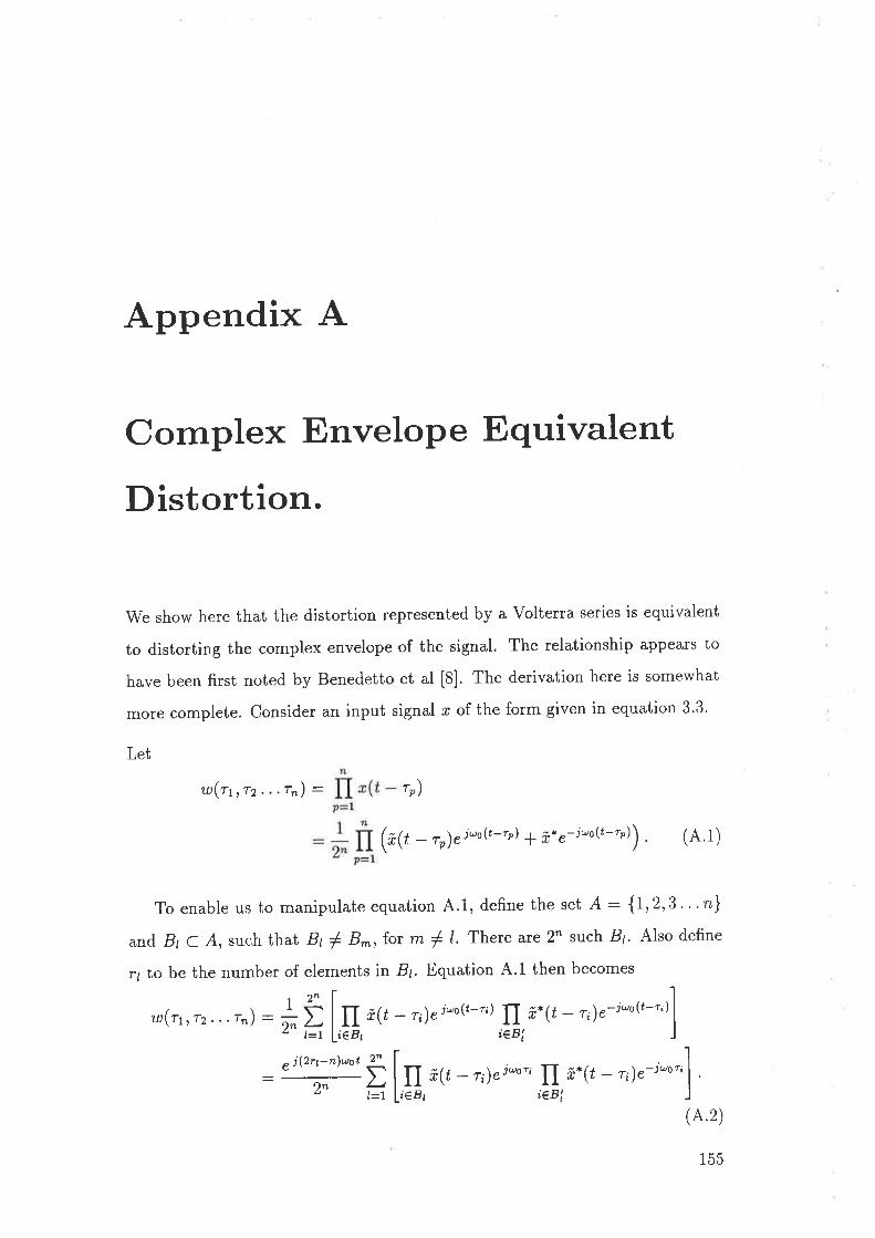
Appendix A
Complex Envelope Equivalent
Distortion.
We show here that the distortion represented by a Volterra series is equivalent
to distorting the complex envelope of the signal. The relationship appears to
have been first noted by Benedetto et al [8]. The derivation here is somewhat
more complete. Consider an input signal r of the form given in equation 3'3'
Let
u(rt,T2. , .rn) : IP )
(rA - rr)ei'o(t-"r) ¡ i*¿-i'o(t-'")) . (4.1)
(A.2)
To enable us to manipulate equation 4.1, define the set A: {1,2,3.. 'n}
and Br C A, such that Br * B*, for m f I. There are 2 such B¡. Also deflne
r¡ to be the number of elements in B¡. Equation 4.1 then becomes
t - r¿)e-i" ('-'t)]
I ¡.(t - rr¡"-i'o''f .
o I=r lieB¡ ieBí I
155
Appendix A. Complex Envelope Equivalent Distortion' 156
Now applying the narrowband constraint, we discard all terms except those
where 2rt - n : Ll. This requires n to be odd so setting n : 2k* I implies
rt: lc * 1 or rt : le . Therefore
w(h,12 '. 'T2k+r) - u'(1,r2..'rn) * w"(rt,rz."rn),
where
,/ , ej-otU (Ír, Tz'.,Tr) :
22k+L Ð Il ¡(t - r,)"i'o". n õ-(t - r¿)e-i'o"illr¿ =fr11 i€Bt ieBi
and¿-iuot
-"(rrrT2...rn):ñ t II ¿(¿ - rn)"i'o"i fI ã.(t - r;)e-i'o';ieB!
(A.3)
We can require without, loss of generality, that the Volterra kernel be sym-
metric [68]. That is to say that å,,(1 ¡r2.. .r,,) remains unchanged for any
permutation of its arguments 1 ¡T2. ..rn and
Ilr¡=k ieB'
Hzp+t : I 1 .. I hr**r(v....rzk+t).'ro*r(rr...rzx+t) d,1d'r2 drnoo
-oo
-ll..lh,r*,(,, rz*+t)wI*+r(tt . . .rz*+t) dr1 dr2' ' 'drn.oo
-oo(A.4)
Now since the value of H2¡¡1 is independent of the choice of the varr-
ables of integration and since hr*+r.(rr,12. . .rzn+t) is symmetric, it follows that
Hz*+t is unaffected by the order of the arguments of w'r¡*r(r1,12" 'r2¡-,'1) and
.ïx+r(rt¡rz...rztr+t).By reordering the arguments of tu'and w", A'3 can be
expressed
tl , ei'ot fl 2k+r I?, \. . ./ : # t . I II t.t' - r¿)e-i'o'; II i(t - r;)ewor;
1o*-' l1r-4+r lr=r i-lc+l I
and
-"(" ):# D ln ã(t -r;)¿i'ott'f .r.r'-';)"-i'"'']' (A'5)!""1' ¿1-rr=¡ ll-Jt i-fr+t I
Appendix A. Complex Envelope Equivalent Distoúion L57
There ut" ('!*t) subsets B¡ such that r¡ : fr, consequently there are ('Tt)terms in the summations in equation 4.5 and they are all equal. Thus
aQ) : I nro*rçxçt¡¡,fr=O
where
Hzr+, : (* i r)# I I ï o**,,,,
k
rzt +t) lI ¿-(¿ - r;)e-ruorii=l
x II ã(t - r;)ei'o"; dr1dr2 . . . drn2k+r
i=kl7
- # I l ,i o**,(', .. rz*+r)fira - r¿)ei'or;
2k+rx II ñ'(t - r¡)e-i'o"; dr1dr2. . .drn
i=fr*1(A.6)
Equation 4.6 is of the same form as 3.3 and so we can write the complex
envelope of y as
û(t) tk=0
('---t)22k l l I o,u*,(,,
co krz*+t) ll ¿.(¿ - r¿)e-ruori
i-1
X Jl ã(t - r¿)ei'o"; dr1dr2. ' .drnzk+r
i-&+1(A.7)
as required.
Appendix B
Multidimensional Orthogonal
Functions
Here we show that the product of single dimensional orthonormal functions are
multidimensional orthonormal functions. This relationship is noted in [67] but
the derivation there is only for the two dimensional case.
First consider all the variables r- to be constant except r¡a. Then we rep-
resent the function f(rt,T2,¡...,ru), as a sum of one dimensional orthogonal
functions l^(rm),
f(rr,rr,. ..,ru) : t a^r(rt,...,ru-t)I^r(ru) (B 1)oo
mM
oo
Now ø-.(tr,.. .,,ru-t) in 8.1, is a function of M - I variables and we
can again consider all the variables r^ !,o be constant except TM-7. Then we
represent the functiort amu¡ as a sum of one dimensional orthogonal functions
l^(ru-r),
a^r(rtrr2,...,ru-t) : D o^*-r^u(\r''' rru-z)lmu-t(ru-t) (B'2)tnM -t
158
Appendix B. Multidimensional Orthogonal Functions
We repeat this process until we have a function of only one variable
159
(8.3)
(8.7)
am2m3...m ¡4("t ) : D o^r^"...^ rl^r(r1).oo
mM
Now we can recursively substitute for d^r(\,,...,ru-t) in 8.1 to get
Drnlootrn7
oo ôo
rnMoo
f (rt,r2,,. . ' ,rv) : t D o*r^r...^ttl^r(rt)I^"(rr) . . .l^r(rrø)m2oo
t D o^r^". .^r0^r,^, ,^¡a(rt,,rz ,Tu),
(8.4)
where
0^r^r...^r(rr, rr . .' rrM) - l^r(rt)l^r(rr) . . . l^r(,*)
We can use a similar tactic to obtain an expression for a^1*2...^¡¡. Noting
that sinceo, fiilj;1, if i : ¡;
then from 8.1
'm2 fnM
(/;(r)/¡(r)) :
a^r(TtrT2r. . ,rr¡ø-t) :
and from B.2
o^r-r^r(Tt ¡ T2¡ ., ., ru-z) :
and from 8.3
arn1m2.,,m¡4 :
By recursive substitution
Il- rfrt,12,- . . ,r¡ø)l**(r¡a) d,r¡a, (B'5)
t: a* r(rt, 12 ¡ . . ., r¡ø -t)l^* -r(r* -t) drM -r,(8.6)
I i o ^,*"...^, (r1) I ^,
(r) d,r1
am1rn2,,,m¡r4 : II Ë .f (rr,rr, '..,r¡rt)
x l^,(r1)l^,(rr) . . . l*r(rv) dr1 dr2 . . . dr¡rt
: ll I:r(,,,,,,...,rM)x þ^r^r..*r(rrrrr. . . rTM) d1 dr2. . . dr¡ø
(B.8)

Appendix B. Multidimensional Orthogonal Functions 160
Equation B.4 shows that the g^r,^r,,,,r(rrrr, . . . ,rM) are a basis and equa-
tion 8.8 shows that they are orthogonal.
Appendix C
Mixers with Sinusoidal Local
Oscillators
Here it will be rigorously shown that a memoryless two input mixer with a
sinusoidal local oscillator, in a bandpass context, is equivalent to a single input
distortion followed by an ideal mixer. The distortion is, however, dependent on
the amplitude of the sine wave.
Let the input be described bY
a(t) : R" [r1t¡" i"']
: t, {rfrl" i'ot * ã. (t)e- i'ot),
and the local oscillator bY
¿(f) - Acos(øf),
: 4, ç",'* * e-i'ot¡
(c.1)
(c.2)
(c.3)
Now let the output be delìned by a polynomial
y(t) : î o*,n*^(¿)¿"(ú).¡n=On=O
161
Appendix C, Mixers wit,h Sinusoidal Local Oscillators r62
Substituting C.1 and C.2 in C.3 and discarding terms except those where rn -2i : !.1 and n - 2lc : fi yields
a(t) : m-l
aþ):
X
Equation C.4 can now be factored
oo
nx t''# çt¡ e. # (t) e@o +' ù i t
XIå o"^*l(n=O
nn-l
e# çt¡tg# (t)e-@o+")it
t* çt¡t'* (t)e@o-'t)it
rv.* (î) : (.#,) which implies th't (,li') : (+). Consequentlv
) (:,) e'f çt1r'#(t)e?'o+'ùit/\2/
Ana^,(+) (+)co
Dm=On=O
nn*l
2Xn
n*1,
1
4
lr* p¡r'* (t)ei'ot "i',t+ ã'+ (t¡r# (t)e-i'o "i'rt+ ft+ þ¡t# (t)et'o "-i"t+ ñ+ (t¡r# (t)e-i'ot "-i"t
v(t) : D Ao^,n n'¿
m-l2rn=O
n=O
n'¿
m-l
(c.4)
(c.5)
x lñ(t)t'(lle--
: /(¿) Ð Ao^,nm=On=0
lx(t)l^ x(t),nn-7
22
as required. Equation C.5 shows the output in the form of the product of the
local oscillator and the distorted signal. Note, however, that the nature of the
distortion is dependent on the amplitude of the local oscillator A.
Appendix D
Recursive Least Squares
Algorithms
In this appendix we will extend the theory of Recursive Least Squares (RLS)
adaption algorithms so that they can be applied to nonlinear filters. Both the
recursive least squares lattice filter and the recursive least squares transversal
filters are de¡ived in a common approach. It should be noted that these are
true least squares algorithms as opposed to algorithms known as "least mean
squares" algorithms.
A linear transversal filter can be divided into two sections. The first part
is the tapped delay line and the second part performs a linear combination of
those taps. A nonlinear filter can be defined where the inputs to the linear
combiner are the terms of a nonlinear polynomial of the :nput samples. The
cost function for selecting the weights in the nonlinear combiner is independent
of how the inputs to the linear combiner where obtained. However, the linear
RLS algorithms achieve computational efficiency by making use of a priori in-
formation about the nature of the inputs to the linear combiner. In particular,
if the filter is defined bV y(r) - e*a(n), then the linear RLS algorithms make
use of the fact that the elements o1 æ(n f 1) are simply those of æ(n) shifted
163
Appendix D. Recursive Least Squarcs Algorithms
along, with the last element removed and a new first element
To extend these algorithms to the nonlinear case, we need to similarly take
advantage of any a priori information on the nature of the elements of æ. For
example, the terms of a nonlinear filter might be arranged as column vectors:
where r; is the input x(t-iT). At the next sampling instant, the values of all the
164
€ 1 €2
delay --€, €,n €u€ 6
r4
Figure D.1: Organization of nonlinear terms into unequal column vectors
columns are shifted right one position. Mueller extended the RLS algorithms
to fractionally spaced equalizers [51]. In his treatment, æ is partitioned into
equal length subvectors. The nonlinear case, when suitably arranged, is almost
of this form if the columns in figure D.l are regarded as the subvectors, except
that the subvectors are not of equal length.
This formulation is useful for nonlinear systems but it is also more generally
useful. For example, consider a linear filter modelling a multipath communica-
tion link. Suppose each of the modes has different dispersion. Such a system
might be modelled acceptably with a minimum number of taps by arranging
the inputs as in figure D.2.
I1I111ï1r11112r112f 2
I11213
r2t212I'2f 21213r2fr3t3
fgrgr313
r5 t6
€ €cs I €2
delay -+ècs3 s4 5 6
r1Itzo
f2rtzt
r3rtzz
&4 Ig I6
Figure D.2: Organization of linear terms into unequal column vectors
Appendix D. Recutsive Least Squares Algorithms 165
D.1 The General Least Squares Problem
Let us define the vector of inputs to the linear combiner by
tæ^(n)*: ( €,("). | €r@). | ... I g-("). ) . (D.1)
For a conventional multiple input linear transversal filter €r(f) ir the vector of
inputs at the lth time interval and {¡(j) : €;-r(f - 1). In the example D.1,
{;(1) are the column vectors. For this general case where the {¿ are not all the
same length,
€,(j) : T;;€;_t(j-1) fori > 1
and
T;:I fori(1. (D.2)
The matrixT¡-t defined in equation D.2 is such that €r(f ) it the same as €;-r(J-1) but with some elements removed and possibly some elements rearranged. We
will derive the properties of ?; more precisely in section D.1.1. The method
followed in this appendix is largely the same that of Mueller [51], however,
the presence of ? in equation D.2 complicates the derivation considerably. Ifequation D.2 is applied recursively
€¿(j) : T;_tT;_2...TÉ,ru -i+t): i¿_r€r(j -i+r),
where
ùr-r, : T;-tT¿-z'''T1
We need to also define a row reduced version of u^(j)
*l^(") = i q,^+q-rÛ o-r,^+r-2''' Û 1,^n^(n)
: Ìq,*+q-tælrt(n)
(D.3)
(D.4)
and
(D.5)
Appendix D, Recursive Least Squares Algoúthms 166
,o^(") : æ*(n), (D.6)
whereT; 00
T (D.7)
0 0 T¡
Where only one subscript is used û'¡ : Ìr,¡'It follows from equations D'7, D'5
and D.3 that
p^ : order({-) (D.e)
and therefore
P^ : order(æ-)
:i0,. (D.10)i=l
The dimensions of the major variables in this section are summarized in table
D.1.
The processes of estimation, forward prediction and backward prediction
are very similar and we will use a notation which allows the derivation of these
three cases in parallel.
The linear combiner is defined by
v',ii@) : c"f (n - I).æl^(n),, (D.11)
where s € {e, b, /} denotes the equalizer, backward predictor or forward pre-
dictor cases. The dimensions of c" : c",0 and g" : y''o are in table D.1. The
00
tJ
*?^-o@)
:-[iJIlï. l€n*,(,+ q). I le^{,+ q). ) (D 8)
That is to say ,o^-o@) denotes a vector made up of the last m - q subvectors
of æ^(n j q).
To keep track of the dimensions of matrices in the following derivation, let
us define
T;+t
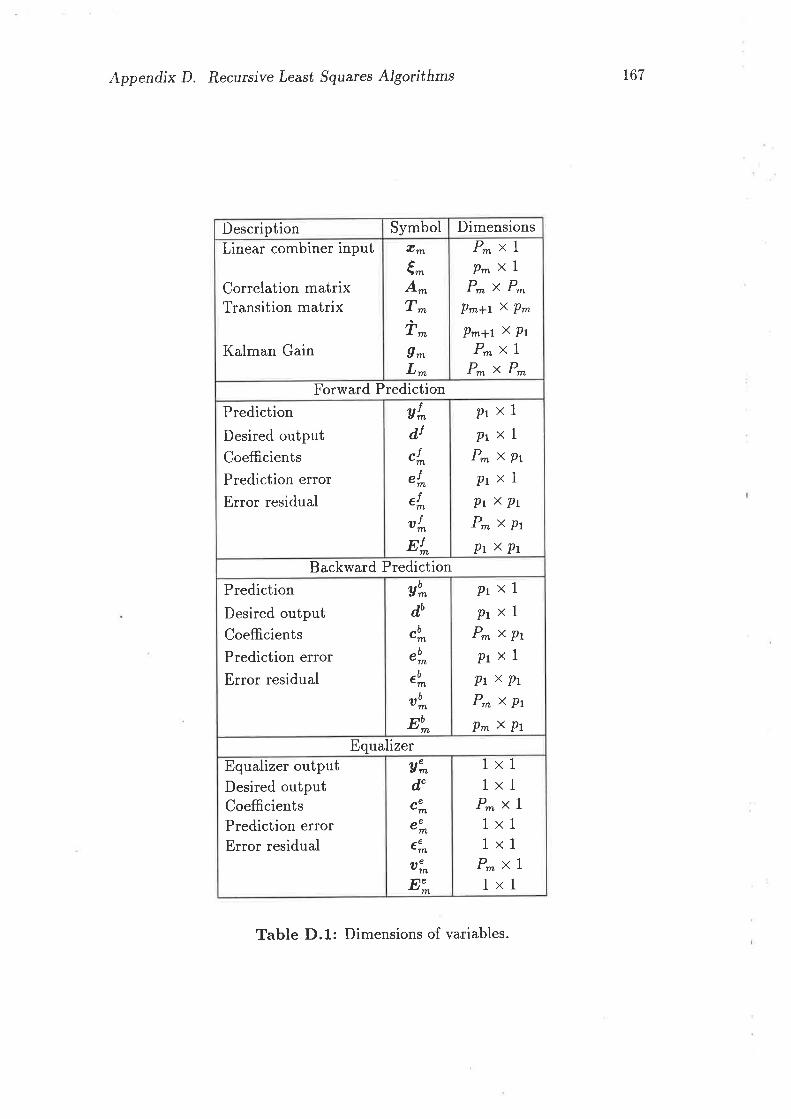
Appendix D. Recursive Least Squarcs Algoüthms 167
Description Symbol DimensionsLinear combiner input
Correlation matrixTransition matrix
Kalman Gain
amcSmA^T^ù*9*L^
P^xIP^xI
P^xP^pm17 X Ptn
Pm+t X PtP^xI
P^xP^Forward Prediction
PredictionDesired outputCoefficientsPrediction errorError residual
gr^
¿rcJrn
er^r
eJn
ar^
Er^
plx!p1xr
P*xPtPrxlPtxPtP*xPtPtxPt
Backward PredictionPredictionDesired outputCoefficientsPrediction errorError residual
Yb^
¿a
cb^
eb^
eb^
ab^
Eb*
plxrPrxlP^xPtPrxlPtxPtP^xPtP^xPt
EqualizerEqualizer outputDesired outputCoefficientsPrediction errorError residual
yidc"*e"^e"^
a"^Ei
1x11x1
P^xI1x11x1
P^xl1x1
Table D.1: Dimensions of variables.
Appendix D. Recwsive Least Squares Algorithms 168
q superscript denotes a member of a family of filters. We are ultimately rn-
terested in the filters corresponding to I : 0, but we need the partial filters
corresponding to q > 0 in the recursive algorithms. Where g is omitted it is
implied that q is zero.
The desired output of the filters are given by
d''*(n): (D.12)
Defining the error as
e",il@) : d^(n) - y",iÍ@), (D.13)
and substituting equation D.l1, we get
.",;f (") : d^(n) - c",if @ - l.æl*(n). (D.14)
Note that the desired output, d", is independent of q.
Equation D.14 defines the error before the coefficients have been updated.
After the coefficients have been updated, we can define a new error
ê',if Ø): d^(n) - c"j(n)-æ1"(n) (D.15)
and a variant form,
é',;f (r,k): di(k) -.',ilØ).r|(k). (D.16)
We want to choose the value of c"ff (n) so as to minimize the mean squared
length of é3f (n,k), 0 < å ( r¿. If êt,tê2,tÊs...êp are the elements of.é'f (n,k),
then the length squared of é!](n,ft) is elei * ezeil eseâ"'epei. Now,
d(r), ifs:ei{t(n*1), ifs-.f;Êt(n-*), ifs:ó.
etelezeiezel
€t€zezeïezei
eteâezeä
ezeié",;l(",k)é'f (n,k)* :
Thus, the length squared of. ëlf (n,fr) is tr(ãfiq (n,k)é'f (n,k)-)
Appendix D. Recursive Least Squares Algoúthms
Let us define the error residual
169
(D.1e)
n
e^(n)"'o: t À"-ké"¡(n,k)é"f (n,k).' (D.17)k=0
The cost function which we wish to minimize is tr(e"'q)^(r). The exponential
factor À is chosen to weight recent errors more heavily than past errors. If the
sYstem is stationaï,r;il;",1; l. ä:::ri::",
ê"j(n).é"](n). (D.18)
The value we wish to minimize is a scalar and it might seem circuitous to first
define a matrix error residual and then define the cost as the trace of that
matrix when we could have simply used the inner product of equation D.18.
However, it turns out that there is insufficient information in the scalar cost
function about the prior state of the system to allow a recursive algorithm'
If the derivative of a matrix is zero, the derivative of each of its elements
must be zero and the derivative of the trace must be zero. Therefore the value
of cif @) which minimizes tr(elq(n)) can be found by found by differentiating
equation D.17 with respect to each of the elements oL cif @) and equating the
derivatives to zero. For notational convenience we drop the m subscript and
the s and q superscripts. Differentiating equation D.17 with respect to c;¡,
ffi: å ^"-r ffiþ@' k)é(n' k)-)
n: ! l"-rfr=0
Differentiate equation D. 16,
ôé(n,k)é,(n,k). * é,(n,k)-ôé(n,k
0c¿,¡(n) ôc;,¡(n)
oe nrlc)0c¿,¡(n)
:mú(k)'and substitute in equation D.19 to get
ffi: å *-r (m)æ@)é(n'&). + lm'@)ë(n'*).] ) (D 20)
: må ^'-0,, k)é(n,fr). + lffiå ^"-0,,
ee"-, Q.)
- o. (D'21)
Appendix D. Recutsive Least Squares Algoñthms
Equation D.21 is satisfied if
170
(D.22)
(D.23)
1L
fr=0
and substituting equation D.16,
D )"-0"(k)é(n,k)* : 0,
Al"(n)c:f (n): a"f (n),
Therefore, returning to the complete notation,
n
k=0
TL
/c=O
which is of the form
where
7I
fr=0and
n
È=0
!.tr"-o la(k)æ(k)-c(") - æ(k)d(fr).1 :0.
Ð À-o rI^Ø)æq^(k). c',;f (") : D À-or|&)dï(k).,É-o
Ai"@): t À-kæ!,(k)*1,&). : ÀAl^(n - 1) + æ1"(n)æ1"(n)- (D.24)
a",;J @) : D À"-k æq^(k)dï(k)- : \a"f (n - 1) + æ1"(n)d}^(n)- . (D.25)
Equation D.23 (together with the definitions D.24 and D.25) is known as the
Wiener-Hopf solution to the problem of minirnizing D.17 [77]'
D.1.1 Properties of the Tlansition Matrices
To proceed further, we need to establish some properties of the Tn,,Ìn and f;Matrices. Recall that {;*r(n + 1) : T;€,;("). Pre-multiplication by T; selects
certain rows of {¿(n) and transfers them to certain rows of €¿+t(, * 1). This is
achieved if ?¿ has the following properties:
l. T; is a rectangular P;+t x p; matrix with p;..1 ( p¡.
2. All the elements of 1; are zero except for at most one element of each
column which is unity.
3. Exactly one element of each row is unity.
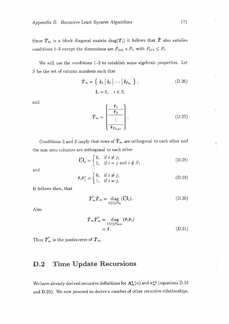
Appendix D. Recursive Least Squares Algoilthms T7T
Since ù^ i" a block diagonal matrix diag(";) it follows that ? also satisfies
conditions 1-3 except the dimensions are P;+t x P;, with P¿+t3 P¿.
We will use the conditions 1-3 to establish some algebraic properties. Let
,9 be the set of column numbers such that
û^:(t,lt,l l¡"-), (D.26)
ûi:0, ieS,and
T (D.27)
î P^*t
Conditions 2 and 3 imply that rows of.ù^ are orthogonal to each other and
the non zero columns are orthogonal to each other
t¿tj : 0, ifilj;1, iLi:jandiÊS; (D.28)
n
and
t,t; : {1,
ifi#j;ifi:¡. (D.2e)
(D.30)
(D.31)
It follows then, that
Also
(t;t¡)
Ì^fri : diag (f¡ô;)1(i(P-11
- I.
fr;Û^: diag1<t'<P-
Thus "i
is the postinverse o1Ì^.
D.2 Time Update Recursions
We have already derived recursive definitions fot Al"(n) and aff (equations D.24
and D.25). We now proceed to derive a number of other recursive relationships.
Appendix D. Recursive Least Squares Algoñthms 772
We find an alternative form for the error residual by substituting D.16 in
D.17
fI
e^(r)"'o : D ^-k ld'^(k) - "",i1@)-æL&)lldï(k) - c"f (n).æå(k)].È=0
IL: t ^-kldï(k)d^(k). - c"f (n)-ui"&)dï(k)-
À=0
- d,"^(k){,(k). c"} (n) -t c",if @)- æL(k)fl&). "# (" )],(D.32)
and substituting D.24 and D.25,
e^(r)"'n: t ^-kd'^(k)d^(k)" -
c'f (n)-u',i1@)n
È=0
- a"f (n). c",ii (") * ci;f (n)- A\".",;f (n),
(D.33)
and substituting equation D.23 in the last term of equation D.33 and simplify-
irg,e^(r)"'o : E'^(n) - a'f (n).c",if ("), (D.34)
where
E"^("): t ^-kdï&)d,ï(k)- : Àtr""*(n - 1) + d^(n)d'^(n)-. (D.35)
,t=0
Now, substitute D.25(recursive form) into D.23 to give
Ai"@)c'f (n) : Àu"f (n - 1) * æ1"(n)d*(n)., (D.36)
use equation D.23 to replace a",;f(n - 1) in equation D.36 to get
Ai"@)c"f (n) : ÀAl(n - r)cif (" - 1) -t æq^(n)d;"(n)-,
use D.24 to get
Ai"@)c"f (n) : lAfi(n) - æq^(n)rl"(").1c:](n - 1)
-l æ1"(n)d}^(n).,: Al^(n)c",;f (" - l) - æ1"(n)æq^(n)-c"; (" - 1)
-f æ1"(n)d^(n)-,use D.13 to get
Appendix D. Recursive Least Squares Algoúthms 173
Al"(n)c'] (n) : Al,(n).",if @ - 1) - æ1"(n)æ1"(n). c"] (n - I)
+ æ1"(n)le',if Ø) + y",;f (")1.,use D.11 to get
Al(n)c'*s (n) : Al,(n)"",;i (" - 1) - æ1"(n)æq^(n)- cff (n - l)+ æq^(n)e"# (r,). + æ1"(n)æi^(n)*c"f (n - l),
and finally, simplify and premuttiply by Al^-'to get
c",;J@) : c",;f (n - 1) + Al,(n)-læ1,(n)e"](n).. (D.37)
Equation D.37 is central to all the recursive least squares transversal algo-
rithms. Unfortunately inverting Al is computationally expensive. We note
that Al^-ræl,is a vector of the same order as æfn. Let us define
' s'^("): Al^(n)-trl^("). (D.3S)
The vector gl"(") is known as the Kalman gain. The Kalman algorithm avoids
inverting At^(") at each iteration by use of the matrix inversion lemma, but it
still requires O(Pf,) operations as it manipulates P* X P- matrices. The fast
Kalman algorithm algorithm is a method of updating gl"(n) without anywhere
ma¡ripulating matrices larger than P* x p;, L < i 1 m. In the linear case
pi:1, and in cases where the fast Kalman algorithm is of interest,p¡ ( P*.
Note that AL-t* - Al*-t since ,Afr, and consequently AL-t, is Hermitian.
We now take the conjugate-transpose of D.37,
"';l (r)- : c'j (n - 1 ). + e'] (n)al^(n)- Al^(n)-t ,
post multiply by a';,f (n), t € {e,ó,/}, to get
c"f (n)-at](r) : c',;l@ - I).utj(n) + e"¡(n¡æl*(n). Al^(n)-latj(n). (D.39)
Premultiply equation D.23 by Al^(")-t and substitute in the last term of equa-
tion D.39 and substitute equation D.25 (recursive form) into equation D.39,
clq(n)-u#(r) : c',;l(, - r¡. [lof (" - 1) + æi^@)d't*(n)-]
* e"f (n)al(n)-ctf (n),
Appendix D. Recursive Least Sguares Algorithms
add and subtract d^(n)dt*(n)-,
c:*q(n)-a#(r) : \c"](n - l)-otf (n - l)
* cij@ - r)-æl^(n)d'^(")- I eij@)æ1"(n)"ctf (n)
+ d^(n)d!^(t,). - d^(n)d!^(n).,
: ),cff(n - l)-atj(n - I)
+ lc"f (n - I)-æq^(n) - ¿ï(")ld'^(")-
r ei;! @)æl^(n). ctj (n) + a;6¡a'^Ø). ,
174
(D.40)
(D.41)
(D.42)
(D.43)
and substitute equation D.14 to get
c"j(n).atj(r) : Àc"f (n - r)-atf (n - 1) - eij@)dt^(n)"
I e'f (n)æ1,(n)-ctf (n) + a;çn¡a'^@)-,
: \c',il@ - l)-atj(n - l)+ e"f (n)læ1,(n).ct;l(") - a'*@l- -f d'i^@)d}^(")-
Put s - ú in equation D.15 and take the conjugate-transpose to get,
é',if @). : d!^(n)- - æl(n)'c',;@),
substitute D.37 to get,
ë';l @). : dt*(n). - æl(n)- ctj (n - 1) - æ1,(n)- Al^(n)-r æl,et] (n).,
substitute equation D.14 for the first two terms
ê',Í(")- : etf (n). - al(n)- Al^(n)-ræ\e',;l(").
: [r - al(n). Al,(")-'rr^) "tif Ø).
: [1 - ti"Ø)].'^,(n).,
where
ú"(") : æ1,(n)* Ao^(")-trl^ (D.44)
Appendix D. Recursive Least Squares Algorithms 175
Substitute equation D.42 for the bracketed term of D.41 to get
c'f (n).atj(r) : Àc"](n - I)-atf (n - l)
- e"] (n)ã|f(r). + d:j (n)d,t*(n).,
and substitute D.43 to get,
c"f (n)-at] (r) : Àc'f (n - l)-atj(n - l)
- [1 - ti"@)]e"](n)et](n). + d*(n)d}*(n).. (D.45)
We are now in a position to derive a recursive form for the error residual.
Substituting D.35 into equation D.34 results in
e^(r)',q : ÀE'^(n - 1) + d^(n)d^(n). - o',if (")-.:,;l(n),
and using D.34 again with n replaced by I - 1'
e",;l("): Àle'f (n - 1) + a",if @ - l).cflq(n - 1)]
+ d'i"(n)d"*(t). - u'](n)"c"](n),
: Àe"f (n - 1) + Àa'f (n - l).clq(n - 1)
+ d"^(n)d'"^(r). - a"f (n).c"](n). (D'46)
Now rearrange equation D.45,
Àc"](n -I)-u'f (n- 1) : c'f (n).a"](n)
+ [1 - tk@\ei]@)eif (r)* - d':^(n)d'*(n).,
and substitute in D.46 to get
e",il @) : Àe'] (n - 1) + lt - tl"(")l e"] (n)e"j (n)".
(D.47)
D.3 The Nonlinear Lattice Filter
In this section we first show that a suitable lattice or ladder structure is equiv-
alent to the transversal structure discussed so far. We then show how a lattice
Appendix D. Recursive Least Squares Algorithms 176
filter can perform orthogonalization of ø and we define some new vartables
necessary for the recursive lattice algorithm'
First consider a quite general nonlinear transversal filter
x!*@) : ø[{, (n) + øiiog,1 n - r) * oii'€, (" - 2)
+...+ oîù¿-r€r(" - i) +'..+ ai-ù^-t€t@ - *).(D.48)
There is a corresponding filter whose impulse response has been reversed in time
and conjugate-transposed. Disregard for the moment the physical significance
of such a filter which is defined by
xb^(") : ùi,-ro^€r(") * ùi-ra^-t€r(" - 1)
* ùi-"a*-r€,r(" - 2)
+ "'+ ùi-o-ro^-¿€,t(, - i)+ ''' + ø,o€,Jn - m)'
Now define reduced order versions of equations D'48 and D.49,
xr^-r(r) : öð€r(") +bîi0€1("-r) +bäÈ1€1(n-2)
+ "' + biù;ftln - i)+...+ bi^-rÙ^-r€r(" - rn * 1),
and
x!*-t(r) : Ùi.-rb^-r€r(") +ùi-"u*-r€r(, - 1)
+ ùi-no^-t€,r(" - 2)
+ "' + ùi-¡b^-;+r€r(, - i + 1)
+ .. .+ öo€r(n - m * L),,
andreplacingnbyn-I,
x!^-r(" - 1) : ùi--rb^-r€r(, - 1) + r;jb^-2{r(n -2)+ ùi-nu^-'€r(, - 3)
+ "'+ ùi-¿b^-¿+ttr@ - i)+ ." + bo€r(, - rn).
(D.4e)
(D.50)
(D.51)
Appendix D. Recursive Least Squares Algorithms
Now take equation D.51 multiplied bV I<f* and add to equation D.50
xr*-r(") + K r*-rx!^@ - t): öi{r(n) + (öîio + I<r^ù;_zb^-t)€r(" - 1)
+ (b;Ì1 + I<r^ù;-sb^-z)ËtØ -2)+ "'+ (bîù,-t + I<r^Ù;-¡b¡n-i+t)€r(" - i)+ ...+ xt*uo¿r(n - m).
(D.52)
Equating coefficients of equations D.48 and D.52
177
Similarly, take equation D.5l and add to equation D.50 multiplied bV I<u^
xo*x!^-r(n) + xb*-t(" - 1)
: r<b^b61't (") + Q<b^bîùo + ù.*_ru*-r)€r(" - 1)
+ 6b^b;ì', + i'.*-ru^-z)Êt@ - 2)
+''' + Q<b^bîù;, + ùi-num-i+r)€r(" - i)+"'+bo€t(, -m).
(D.57)
Equating coefficients of equations D.49 and D.57,
and
a[: b[,
okù^-r: I<Í^bs,
aiù ;-t. : bîù ;-t + I< r^ù;-ib^-i+t,
xr^(") : x!^-t(") + K r^x!^-r(" - 1)
ao : bo'
ùi-ro*: Kb^bå,
ùi--,-ro^-i : Kb*bîù,-, + ùi-ob^-n*r,
(D.53)
(D.54)
(D.55)
(D.56)
(D.58)
(D.5e)
(D.60)
and
x!^@) : Ku^xr^-r(") * xb*-r(" - 1). (D.61)
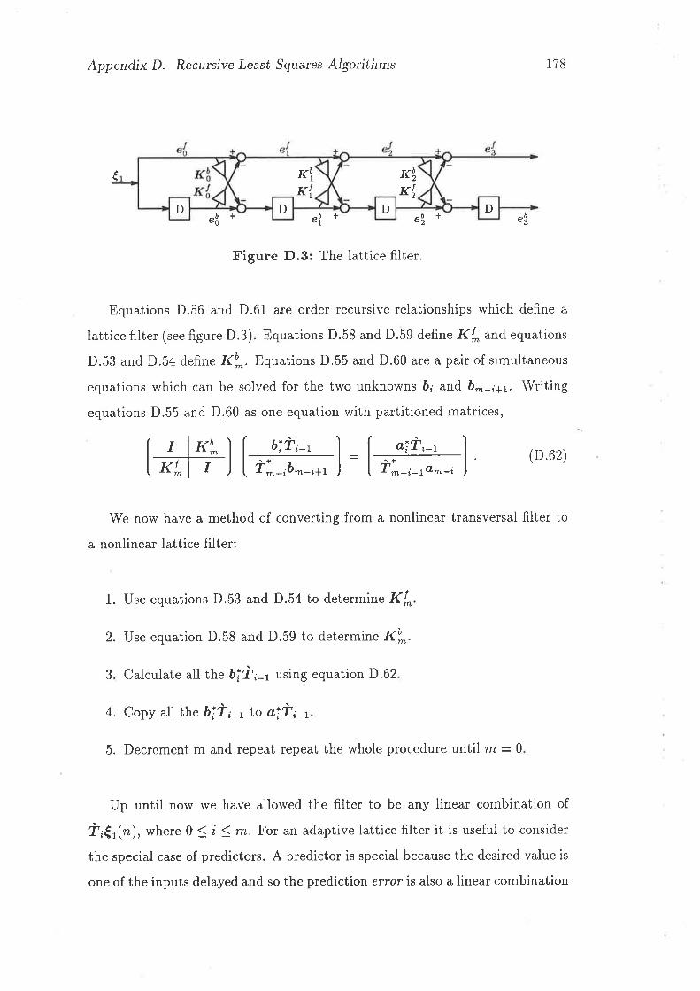
b1
¡1
I{I{
rtb,KI
DD D D
Appendix D. Recursive Least Squares Algoúthms
e$ e\
178
è
+ + eb2 + eb3
Figure D.3: The lattice filter.
Equations D.56 and D.61 are order recursive relationships which define a
lattice filter (see figure D.3). trquations D.58 and D.59 defin" I<i^ and equations
D.53 and D.54 defin" I<b^.Equations D.55 and D.60 are a pair of simultaneous
equations which can be solved for the two unknowns b¿ and b--;-,.1. Writing
equations D.55 and D.60 as one equation with partitioned matrices,
fAELl I .,u;T'-' l: f ,:&Ll (D62)lI<'^l I )lT*-nbm-i*r J tT^-¿-ta*-i)
We now have a method of converting from a nonlinear transversal filter to
a nonlinear lattice filter:
1. Use equations D.53 and D.54 to determine .tffl
2. Use equation D.58 and D.59 to determine .üfl.
3 Calculate all the biù;; using equation D.62
4. Copy all the öîÌr-. to aiù;-1
5. Decrement m and repeat repeat the whole procedure until rn : 0
Up until now r¡/e have allowed the filter to be any linear combination of
i,€r(r), where 0 < i < rn. For an adaptive lattice filter it is useful to consider
the special case of predictors. A predictor is special because the desired value is
one of the inputs delayed and so the prediction error is also a linear combination
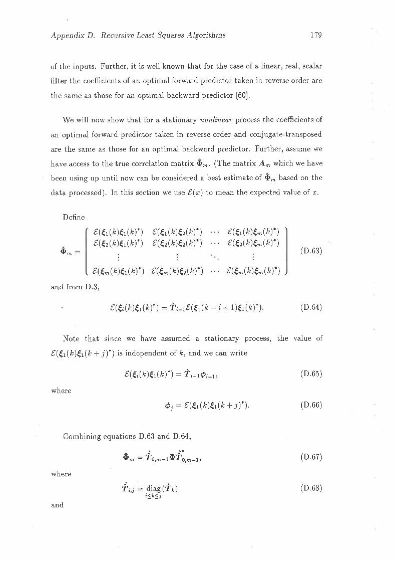
Appendix D. Recursive Least Squares Algorithms 179
of the inputs. Further, it is well known that for the case of a linear, real, scalar
filter the coef;Êcients of an optimal forward predictor taken in reverse order are
the same as those for an optimal backward predictor [60].
We will now show that for a stationary nonlinear process the coefÊcients of
an optimal forward predictor taken in reverse order and conjugate-transposed
are the same as those for an optimal backward predictor. Further, assume we
have access to the true correlation matrix ô-. 1th" matrix A- which we have
been using up until now can be considered a best estimate of ô- based on the
data processed). In this section we use t(r) to mean the expected value of ø.
Define
o
t(€1(k)€r(/c).)tG,(k)€r(k).)
(D.63)
and from D.3,
t(€¿(k)€,(k).) : Ù¿_rt(€J(k - i+ 1)€1(fr).) (D.64)
Note that since we have assumed a stationary process, the value of
t(€t(k)€t1k + r).) is independent of k, and we can write
t(€;(k)€r(k).) : ùo-,,ó;-r, (D.65)
where
ó¡ : t(t'(k)€'(k + i).). (D.66)
Combining equations D.63 and D.64,
(D.67)
where
Ì¡j : diag (i¡)i<h<i
r(€1(k)€l(k).)r(€r(k)€1(k).)
r(€1(k)€-(k).)t(Ër(k)e*(k).)
rn
and
(D.68)
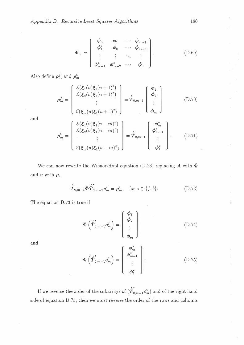
Appendix D. Recursive Least,Squares Algorithms 180
óoói
óróo
óó
m-lm-2
Õ-: (D.6e)
ók-' ói--, óo
Also define pr* and pb*
t(€,(")€,(n + 1).)t(€r(")€,(n + 1).)
ó,
-T O,rn-I (D.70)
t(Ë^(")Êr(n * 1).) ó^
t(€r(")€,(n - rn).)t(€r(")€r(n - rn)")
_ al1
- r O,m-lQ^-7
(D.71)
t(€-(")€, (" - ^)-),
We can now rewrite the Wiener-Hopf equation (D.23) replacing A with ôand o with p,
^t ^t*To,^-iÞTo,*-{T: pT, for s € {f ,b}. (D.73)
The equation D.73 is true if
ó,fP'*
andQ-
Qt
Pb^
ótó,
ó^
Q^ói"-t
" (i,,--,"1)
" (ô,,--,"1)
(D.74)
and
(D.75)
Qt
If we reverse the order of the subarrays of (fs,--1cl) and of the right hand
side of equation D.75, then we must reverse the order of the rows and columns

Appendix D. Recursive Least Squarcs Algorithms 181
of iÞ which is equivalent to taking the conjugate-transpose of each of the sub-
matrices of iÞ (refer to equation D.69). Define o/ and a| such that
c and cb*("¡ : (D.76)
a
ou^-ù^-'d.
*ù*-z
o{o.r,
d.
d.
ab^
b1
b2Í
rn n
fn'¿
Consequently,
ótóz
ó^
obm-l
ol.ÌoComparing equations D.77 and D.74,
ùi-ro{ -- ob^+r-o ù*-;,,
as required.
From equations D.14 and D.12
.r,,("): €r(n + l) - cr** æ*(n)
: €r(n + 1) + d{.€l(n) + arr. ¿r(n¡
+...+ ot^.e^Ø)
: €r(n + 1) + a{-i'.o€,r(r) + d[.ùL€r(" - 1)
+' " + dl^.ù*-rË,r(, - m * L),
er^Ø - 1) : {r(rz) + c{.?og r(, - r) + ar2.ùrÊ,r(" - 2)
+ . .'+ of^*Ù^-r€,r(, - *),
which is of the same form as D.48. Similarly
"b^("): €r(, - m) - cb,*t^(n)
: Êt(n - r7-) + aï.€1(n) + o,br. fr(n¡
+...+ db*-f"^@)
(D.77)
(D.78)
(D.7e)
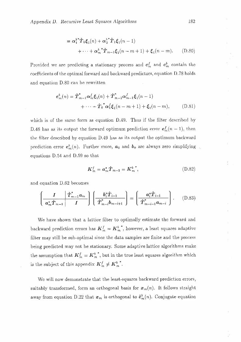
Appendix D. Recursive Least Squares Algorithms 182
: af.is{r(") + our-ùrËr(" - 1)
+ . . . + db**ù*-r€,r(n - m t 1)+ €r(" - m). (D.80)
Provided we are predicting a stationary process and cÍ^ and cf; contain the
coefficients of the optimal forward and backward predictors, equation D.78 holds
and equation D.80 can be rewritten
eb,,@): i'i-ror^€r(") +ùi-rar^-r€r(" - 1)
+ ... + ùo. a{Êr(, - *+ 1) + Êr(n - *),
which is of the same form as equation D.49. Thus if the filter described by
D.48 has as its output the forward optimum prediction error el^(n - 1), then
the filter described by equation D.49 has as its output the optimum backward
prediction ercor eb^(n). Further more, úús and bs are always zero simplifying
equations D.54 and D.59 so that
(D.82)
and equation D.62 becomes
I{r^: oi^ù^-, : I{u^* ,
(D.81)
(D.83)I lT^-ta*aî-ù^-t, I r
We have shown that a lattice filter to optimally estimate the forward and
backward prediction errors has Kl^: Ko^*, however, a least squares adaptive
filter may still be sub-optimal since the data samples are finite and the process
being predicted may not be stationary. Some adaptive lattice algorithms make
the assumption that ltr^ : I{b^*, but in the true least squares algorithm which
is the subject of this appendix I<r^ + I<b*-.
We will now demonstrate that the least-squares backward prediction elrors,
suitably transformed, form an orthogonal basis for æ*(n). It follows straight
away from equationD.22 that a^ is orthogonal to ¿o^("). Conjugate equation
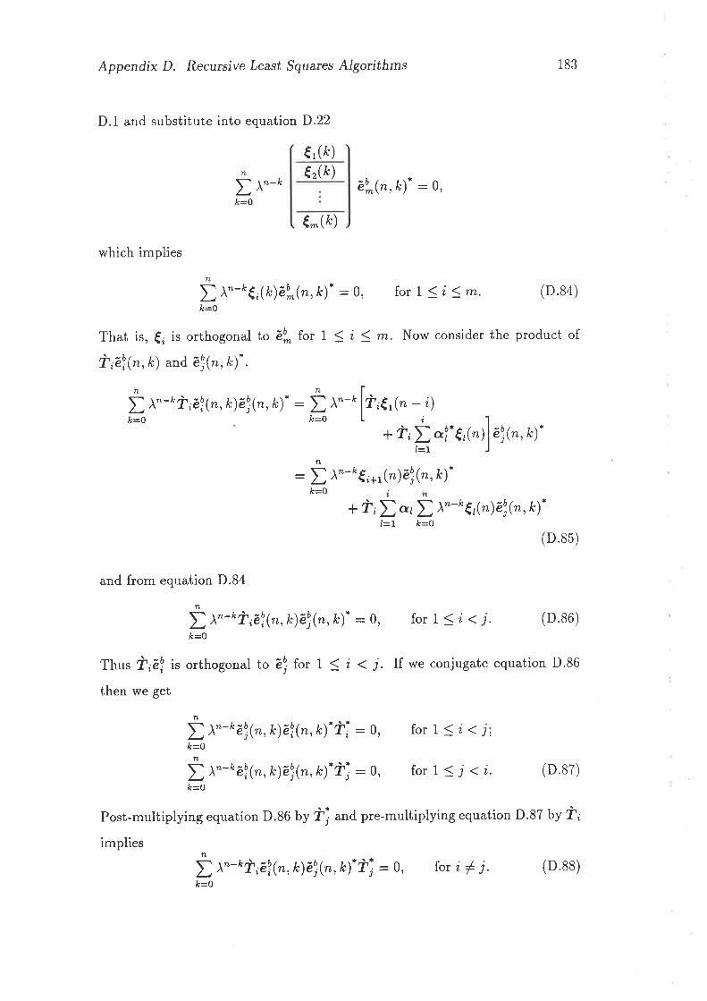
Appendix D. Recursive Least Squares Algoúthms
D.1 and substitute into equationD.22
183
(D.85)
€,(fr)n
,t=0
er&)D À"-o ¿u^(",k)* :0,
€-(fr)
which implies
n
Dl"-*€,(Qeb^@,k)*:0, for 1( i1m. (D.84)
That is, {¿ is orthogonal to éb^ for 1 ( i 1 m. Now consider the product of
ù ¿e!1r,,k) and él(n, k)- .
&=O
n
/c=0
and from equation D.84
n
,b=0
n
ÉA=O
À^-o €n+r(r)él(n,k)-
*i;fo¿ tlc=0
n
D l"-*io él(n, k)ã:b¡(r, k)* : | À"-r' ù,€,r(" - i)fr=0
* t,Ð o!. ¿,ç,¡)e]{, ).
^-k eín)éu,{",*¡-
k
I=l
! l"-Èir e!@,k)él(n,le)* : Q, for 1 ( i < i. (D.86)
Thus f;ãf is orthogonal to él for I < i < i. If we conjugate equation D.86
then we get
Dk=0
TLtfr-o
À-kéb,(n,k)ébn@,k).ii :9, for 1( i<i;
À"-ké!(n,k)éb¡(n,,*)-ùj :0, for 1 ( j <i. (D.87)
Post-multiplying equation D.86 by i¡ ,"d pre-multiplying equation D.87 by ?n
f À"-*f, ël(n,Ðébj(n,k).ùj :0, ror i I j. (D.s8)
implies
ic=O
Appendix D. Recursive Least Squares Algorithms
Now from equations D.15 and D.12,
¿o^("): Ér(r - m) - cb^(n)- æ^(n)
and
ù ^éb^(") : €rn+l (") - ù ^.b*ç"¡- æ^(n)
:(-i-c11"¡-lr)€,^(")
€*+t(n): ( -ù^.b^(r)- | r ) r-1'("¡.
-focå n)
-f 1cl(n).
184
€'(")ë,r(")
æ^+t(n). (D.89)
(D.e0)
Therefore
where
ùoéooØ) 0Iùr¿l(") 0
ù^¿o^(") -ù*cb^(n)- I: L^(n)æ*(r),
-Ì6cf (n). I 0
-i1cl(n)- (D.e1)L^(n):
-'i'*-1cb-r(n)* ISince t¡. ù;éb;(") are a linear combination of the €,*(n), they span the same
space so long as L^(n) is of full rank. Thus pre-multiplication by L^(n) has
orthogonalized æ^(n). In a sense, this is only a partial orthogonalization. The
subvectors ùré!(") are orthogonal to each other, but the elements of (¿ are not
orthogonal to each other. This is, however, the best that can be achieved by
the lattice structure.
Now define a transformed input vector
t^(n)- L^(n-l)æ^(n),
0
where
(D.e2)
Appendix D. Recursive Least Squares Algoúthms 185
ú^(n): (D.e3)
E^@)and from equations D.91 and D.14,
e^@) : 'i'^-reb^-, (r). (D'94)
In this case, the sub-vectors of.ú^(n),(^,, ut. not truly orthogonal, though for
a stationary process and sufficiently large n they will approach orthogonality.
In the lattice based equalizer algorithm we define the output to be a linear
combination of ã.
Let us define Ã("¡ ""
É'(")trØ)
n
Ã*("): D \"-k L^(n)æ*(k)æ^(k)* L^(n). (D.e5)
(D e6)
(D.e7)
&=0: L^(n)A^(n)L^(n)*
We can partition å(n)al,L at2 (1r,m
@z,t az,z Ø2,m
Á.^çr¡:dm,l am,2 a^,rn
where (from equations D.90 and D.96),
o,i,j : ! À"- ß ?r -ré! -r(n,, k)ëu¡ -r(n, k). ù] -t,&=0
and from equation D.88,
Ai,i 0, forilj
Thus,
A^(n): diag71i1m-l
and from equation D.17,
(t,-, lå ^"--ut -,(n,k)é!-,(,,*).] r;-,) ,
Á.^çr¡: diagO(i(r¿-1
(r,.i(")ii) . (D.e8)
Appendix D. Recursive Least Squares Algorithms
Equate the right half sides of equations D.95 and D.98
L ^(n) A^(n) L ^(n)- : 0.,41ï8_, (ir.! (")il),
pre-multiply by L^(n)-1 and post-multiply by ll*(n)'l-t ,
A*(r) - L^(")-'o.d,.lïs_, (ro.l(")ii) lt ^ç"¡.1-' ,
and invert,
A*(n)-' - L ^(,). o.glïs_, ( [i,.3 {") à;] -' ) L ^@)
Now the equalizer output is a linear combination of õ
gi(") : ô"^(n - L)* i^(n),
and from equation D.11,
ci(" - l). æ^(n) : õ"^(n - I)- ú*(n)
: é"^(n - L). L*(n - l)ñ^(n)
Equation D.101 is satisfied if
ci(" - 1)* : ¿i(" - l). L^(n - l)
¿ï("): L^(r)*-t.ï(").
Apply equation D.23,
¿ï(") : L^(n)*-t A^çr¡-'oï("),
186
(D.ee)
(D.i00)
(D.101)
and substitute equation D.99,
¿ï(") : L*(n)*-t L^(r)' diag ( lt,.ir"lt;] -') L^@). ai@)
O1i1n-l
(D.102)
Take the conjugate-transpose of equation D.102, replace n with n - 1, and
substitute into equation D.100,
si@) : (L^(n - r)a"^(n - 1)).
,.*lïr_, ( [t,.] r"lt;] -') L *@)a"*(n).
diag0(i(rn-1
X ([t,.ir" - 1)i;]-') r*@) (D.103)
Appendix D. Recursive Least Squarcs Algorithms
Let
ll^(n)ai(r)1. : ( ,'(r). l.r@). I
and substitute into D.103 to get
sï("): ( z{n)-
.^Ø). )
187
(D.104)
)1\)ã^(")'
2 ("). 1 . ..1"^@)-
([t,.lt" - 1)i;]-X diagn'L -0l 1
and substitute D.93 to get
i=1
i=l
[:r,.?(n - 1)iî]-' t,@)sï(") : ( z{n - 1). l.r@ - 1). | .. )
: Ë ",(n - 1). [i¿-1e! -r(, - 1)Ì;-,]-'Ê,(r,),
and from equation D.94
vï@): t ",(n - 1). [f;-rel-,(' - 1)i;-,]-' ùn-,"un-ri")i=7
:irnçn- r). [i;- ,el-r(n- 1)f;-,]-' ù^-,.u*-r(n)
: yï-tØ) * z*(n- 1). [Ì-- çb^-t@ - Ðù;-,]-'x ù^ae nb
m-7 ( ) (D.105)
Equation D.105 is an order recursive form for calculating the equalizer
output yï(n). It depends however on being able to calculate z*(n - 1)*,
eb^-r(, - 1) and .b*-t("). We proceed now to find a recursive form for
t*(n - 1)..
From equations D.104 and D.91,
,*(n) : ( -ù^-r.b^-r(n). l t I o ) "ï@)From equations D.l and D.25,
,^(n) : ( -ù^-rcb*-r(r). l t I o )
Appendix D. Recursive Least Squares Algoilthms
and substitute equation D.45 to get
z^(n) - -^ù^-,,cb^-r(, - r)* oï-r(" - 1)
+ [1 - 1 ^ -t(n)] ù ^ -reb*-r(n) e'^ -r(n).
188
- ù^-rdu^_,.(")dï_r(rr). + I À"-*€- (k)d^(k)-n
,b=0
À -ù ^-rcb^_, (r - r). oï_r(" - 1) + t ¡n-t-* ¿^çk)d^(k).
n-l
,t=0
+ t^&)dï(k). + lr - -'-._,(n)lÙ^-teb*_rçn¡e;_rç"¡.
- ù ^ - t
d'* -, (n) d* - r(n).
- Àz^(" - 1) + [1 - l^-t(")]ù^-,,.b^-r(n)ei-r@).+ t *Ø)dï( k). - ù ^-,,d0*_r(n)d,i_r@).,
and note that d,"^(n) - d*-t(n) (equation D.12) to get,
z^(n) : Àz^(n - 1) + ll -'t*-r(n))ù^-1eb^-r1n¡e7-rçn¡-+ [€-(") -ù^-rd!^-,(")] dï@)-
: Àz*(n - 1) + (r - l^-r("))ù^-teb^-rç")e2-r(r).+ [€-(") -ù^-rdu^-,(")] dïØ)..
From equation D.12,
dþ^_,,("):€r(, -m*L)
and, applying equation D.4,
ù^-,,db^-r(r) : €,*(")
and substitute in equation D.106 to get
,*(r) - Àz^(" - 1) + [1 -',t^-t(n)lù ^-reb^-r(n)e"^-r(n).
(D.106)
(D.107)
Appendix D. Recursive Least Squares Algorithms 189
D.4 Order Update Recursions
In this section we derive order update recursive relationships, effectively describ-
ing a filter of length rn in terms of a filter of length m - I. These relationships
are clearly necessary for a lattice filter. They will also be necessary for the fast
RLS transversal filters.
Define€'(")
€'(" - 1)(D.108)ù^(n):
€r(, - m-ll)From equations D.l, D.3 and D.68 it follows that
(D.1oe)
Now
ù^(n):
and from equation D.12,
ù^(n):
Similarly
ù^(n):
and from equation D.Lz,
ù^(n):
Also define
t#,#l (D.110)
(D.111)
Â^(") : t ^-k û^(k)ô^(k)-
n
andfr=0
(D.112)
Appendix D. Recursive Least Squares Algoúthms
î,'^(" + 1). Eb^(n + L)
190
(D.113)
(D.114)
(D.115)
(D.1i6)
(D.117)
1 18)
(D.11e)
oï(") : t ^-k ù^(k)d,i(k)-
n
Å=O
From equations D.24, D.109 and D.112
Similarly, from equations D.25, D.109 and D.113
am: ùo,^-rû^.
From equation D.110,
û,^+r(k)&^+r (k). : ù*(k)ù^(k). û^@)db*Ø)-dþ*(k)ù^(k). db^ft)dþ^&)-
and substituting in D.112,
À^+t(n * i) :Â^(n + t)
"f ¡"*t-o db^&)ù^(k)-À=0
"f ¡"*t-* û^(k)db^(k)"å=0
"f ¡"*r -o db^(k) d!*(k).,t=0
and applying equations D.113 and D.35,
Â^*r(r* t) : I
Â^ n*I ob^(n + t)
Similarly, using equation D.111,
û^+{lc)ù^+t(k). :
Consider an arbitrary function f (*,,k),n*l n
| À"+t-tt(m,t - t) : D À"-ol(rn,k)l=o 'b=-1
bysetting le :l-I,n*7 n
!À"+t-rt(*,1, - 1) : \*tf(*,,-1) + tÀ"-ol(rn,k).À=0 å=0
Setting f (*,k - 1) : ù^+r(k)ù^+t(k). and applying equation D.112,
D(
Â^+t(n + 1) - \+7ñ^1.r(0)ô-*r(0). + D ^-nù^+t(fr * 7)ù^+t(/c + t)-
n
&=0
Appendix D. Recurcive Least Squarcs Algoúthms
and, provided ô-..,'1(0) : 0,
191
n
Â^+t(n + 1) : D À"-kû^+t(k + la^*l(fr + 1).À=0
Substitute equation D.118 with ,t replaced by fr * 1 to get
Â^+t(n * 1) :i l"-o ¿t &)dr^&).
È=O
i ¡"-x ù^(Ðdr^$).
i À"-o¿t &)ù^(k)-À-o
i ¡"-n ù^&)ñ*(k).,b=0k-o
and applying equations D.112, D.113 and D.35,
Â^+t(n * 1) : (D.120)
We now use equation D.120 with rn replaced by * - 1 to substitute for
A^(, * 1) in equation D.117,
Er^-r(")- i,f^-r,(").ûo^(" + 1)i;
Â^+t(n * 1) : î'r^-r(") A^-t(r) (D.121)
î,u*(" + 1). Eb^(n + \)
From the definition of ô- (equation D.113), and equation D.111
o'*("+1) :f¡"+t-r'n*t
ic=0
dþ*(k)-,
and from equation D.Iz,
(ån1, 1)+na
(D.122)
Note from equation D.12 that d!*&) = db^-r(k - 1), and also apply equation
D.119 to get
nllD )"+t-rgr(fr)€r(k - *)*À=0b
n1. 1)+ TLa n
Àn|t ù * _,.(o)dl_l (o). + Dfr=0
À"-kû^-,.(Ðdb^_Jk)-
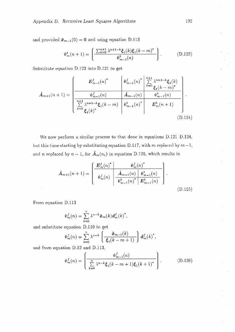
Appendix D. Recursive Least Squares Algorithms
and providedû^-1(0) :0 and using equation D.113
itt^-r(")-
îto^_,,(")-
i,o^-t (")
r92
(D.123)
(D.125)
(D.126)
tu^(" + 1) :
Substitute equation D.I23 into D.121 to get
Et^-r(").
Â^+t(n * 1) : îtr^-r(")n*lD l"+t-trr(k - -)*=o
€, (k).
Â^+t(n * 1) :
n*.lD À"+t-o€r(fr)
o=o €r(k - *)*
Eb*(n + t)
(D.124)
We now perform a similar process to that done in equations D.1,2I-D.I24,
but this time starting by substituting equation D.117, with rn replaced by m-I,and n replaced by n - 1, for Â^("r) in equation D.120, which results in
Et^("). a'^lnÂ,^ (")-1 tu^-r(")
0t^(")ûo*_r("). | "u^_r(")
From equation D.113
or^("): D ^-k ù^(k)d,r^&). ,
n
À=0
n
,t=0
and substitute equation D.110 to get
or^("): ! ¡"-* d,t^&). ,
and from equation D.12 and D.113,
îtl^-r(")ttt^67 : n
DË=0
À"-߀,(ß -m* 1)€,(fr + 1).
,q^-t(r)
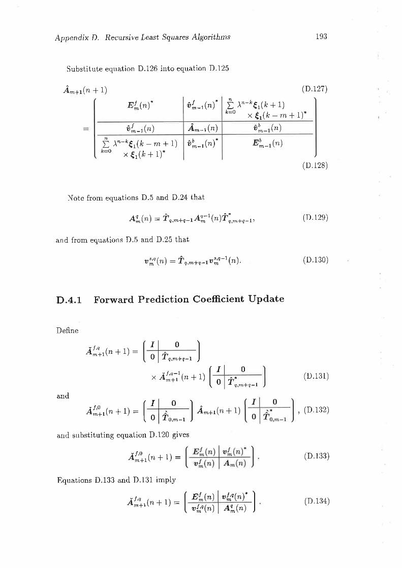
Appendix D. Recursive Least Squares Algorithms
Substitute equation D.126 into equation D.125
A^*t(n + t)
nt^@)- û'r^-r(").nD
lc=0
î,1^-r(")
É r"-*€r(k-m*t)t=o x€r(k+1).
Ã'^o*r(n* t) : I
I o
0 ^'To,^-lÁ-*t(r¿ + t)
193
(D.r27)
(D.128)
(D.12e)
(D.130)
(D.131)
, (D.i32)
(D.133)
À"-fr€1(k + 1)x €r(k - rn * 1).
a
Eb^
b (")n
(")t'o^-r(')-
Note from equations D.5 and D.24 that
Ai^@) : fr q,^+t -1 Al;r @)ti,^*o-r,
and from equations D.5 and D.25 that
a',;J Ø) : ù q'^+q -t tt#-t (')'
D.4.L Forward Prediction Coefficient Update
Define
rl 0ArÅo*r("+ 1) :
0 lfn,^*o-, rl 0I^*
O lTo,**o_,and
and substituting equation D.120 gives
Ã'^o*r(n * 1) :
Equations D.133 and D.131 imply
nr^@) ar¿e@).
A^-t(n)
Ãr*o*r('+ 1) :ako(") I tLØ) (D.134)
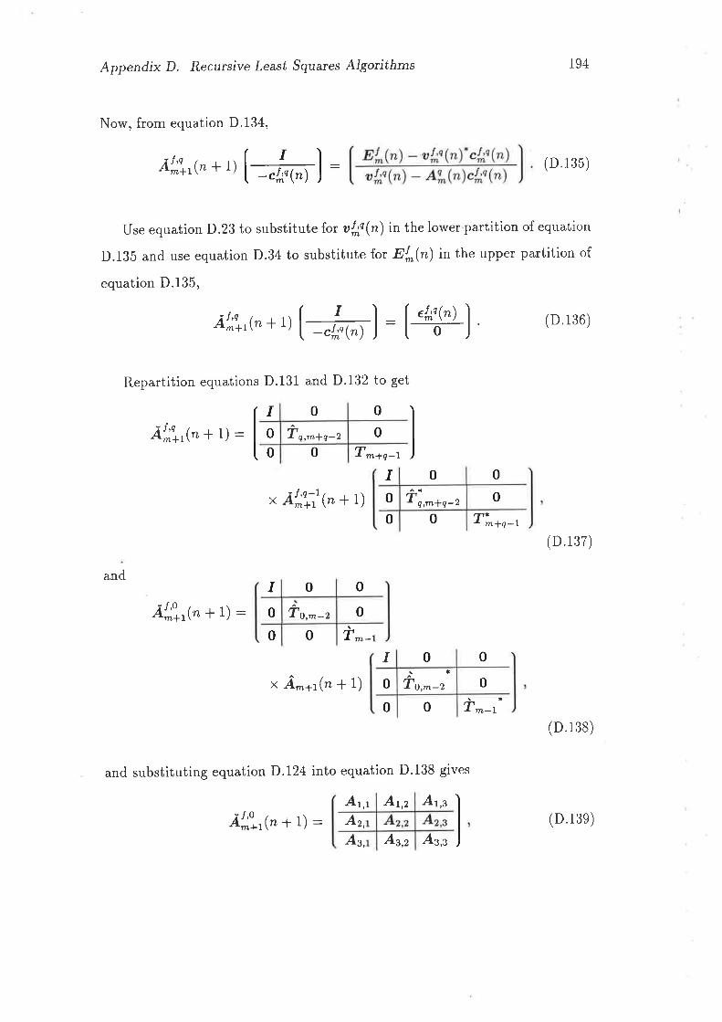
Appendix D. Recursive Least Squares Algoüthms
Now, from equation D.134,
r94
Use equation D .23 to substitute for " ko (") in the lower partition of equation
D.13b and use equation D.34 to substitute for Er^(n) in the upper partition of
equation D.135,
Ã*\,(n+1) t=#J : [4#Ù] (D136)
t=#o_1Ãt;'*r(n + 1)
T^-t
(D.135)
(D.137)
(D.138)
(D.13e)
Repartition equations D.131 and D.132 to get
0
Ãt;\r(" + 1) : 00 0 T^+q-7
0
0I
x Ãr;\r'1" + t¡ 0
I 0
0
0 0 Tk+q-t
0
and
Ã'^o*r(n * 1) : 0
I 0 0
0
0 0 ù0
x Â^+t(n + 1) 0
0 0
and substituting equation D.124 into equation D'138 gives
1m-
0
0
I
Ã!Åo*r(n * 1) :At,Ao
I At,z At,z
T q,mlt-2
Ì|,^+n-z
To,^-z
^t*To,^-z
43, Ag,z Az,s
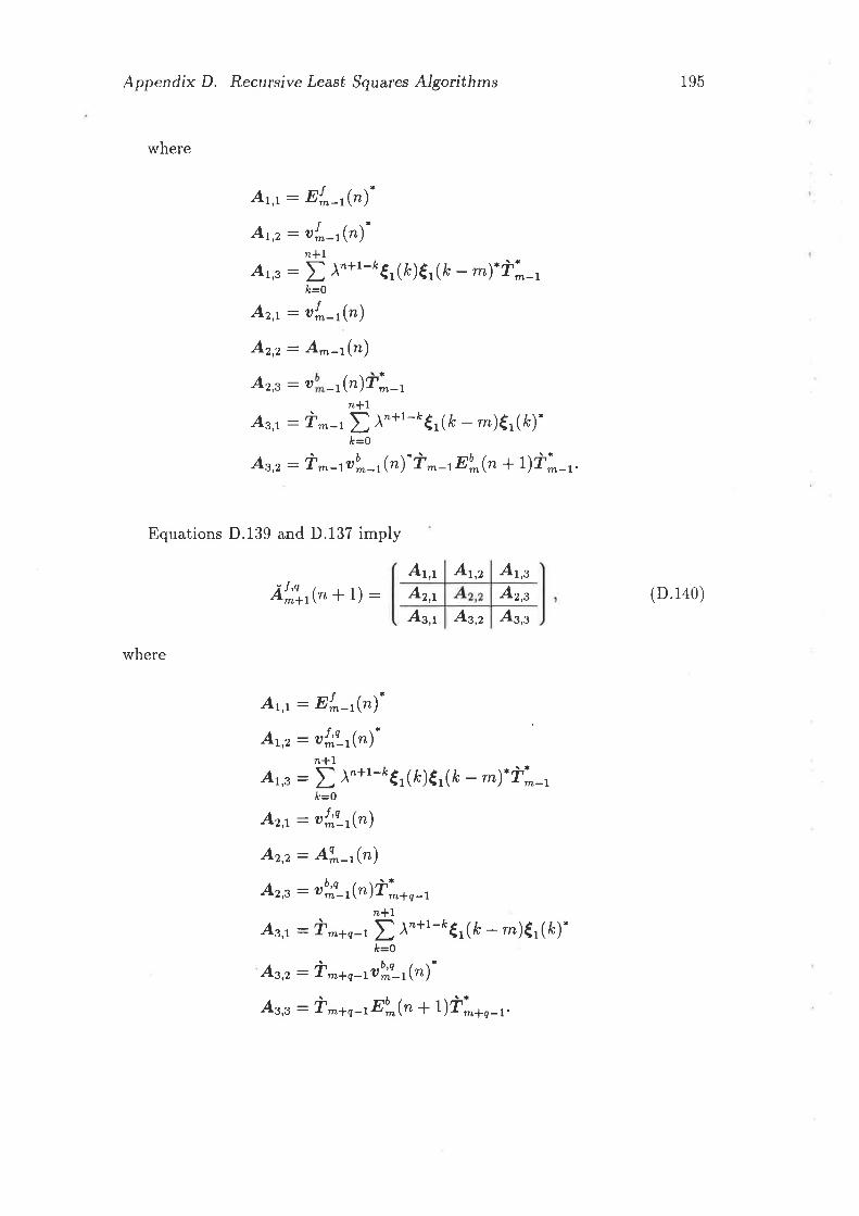
Appendix D. Recutsive Least,Squares Algoúthms
where
195
(D.140)
AtJ: El^-r(")-
At,z: of^-r(r)-r¿*1
ALþ : | À"+t-r*r(fr)€, (k - @-ùi_,/c=0
AzJ: or^-r(")
A2,2: A^-r(,)Az,s: u -r@)ùi-,
n*7Asr: ù*-t ! À"+t-*rr(ß - -)€r(fr).
/c=0
Az,z : ù ^ -rob^ -r(n)* ù
^ -1 E'^(" + 1)ù; -r'
Equations D.139 and D.137 imply
At,t At,z At,eÃ!;o*r('* 1) : Az,t
Az,t Ag,z
Az,e
As,z
where
AtJ: Er^-r(r).
At,z: a!Åo-tØ).r¿*1
At,e : ! À"+t-r'r, (k)€r(È - *). Ù.^_,å=0
A2J: ako-l@)
Az,z: Al"-t(")Azp: "b¡-rç"¡ùi.+o-,n*1AsJ: ù^+q-t ! À"+t-r'r r(k - -)€r(fr).
È=0
A3,2 : ù*ao-rabff-r(r)*
A'¿,s: ù**n-rÛb^(n + \ùi*o-r.
Appendix D. Recursive Least Squares Algorithms
Therefore,
196
Ãr;\r1" + t¡
l-rk'-r(r)..0,Í-r(r) +'f ¡,*'-o€,(fr)€, (k - *f]ùi*o-,l- oi, -, (") "!,il_ r( " )
+ r',ä- r@)] ùi * o _,
ù^+q-tl-"u,1:-r(r)- "0,Í-r(") + Eo^(" + 1)] r;+r-l
(D.141)
We can put equation D.141 into a more tractable form if we definen*l
ko,;l-r("): t l"+t-߀r(k)€r(k - *)* - at*n-,,(n)- cbff-r(n). (D.r42)Ë=1
From equations D.35 and D.12
Eu^(r+ 1) : $ ^'*'-o€r(k - *)ër(k - *)*,
/c=0
and using D.119
Eo^(n+ 1) : À'+1€r(--)€,(--). + Ë À'-fr€r Ø - *+ 1)€, (k - *t 1).,&=0
and provided {r(n) : 0; for n ( 0,
Eo*("+1) : Eo^-t("),
and using equation D.34
Eu^(" + 1) : ,b,i!-r(") * ou,il-r@). cbff-r(n).
Substitute equations D.23, D.142 and D.143 in equation D.141,
(D.143)
0
Ãr;\rç" + t¡ -.b,i!-r@)ùi¡o-r
(
ID 441
Now substitute equation D.128 into equation D.138 to get
At,sAz,t Az,zAt,t At,z
Ã'Åo*r(n * 1) :,4s,r As,z Az,z
(D.145)
Appendix D. Recursive Least Squares Algorithms
where
197
(D.146)
At,r: nr^@).
Ar,2: ar^-r(n)-n
Atp : Ð .1"-n€r(/c + 1)€1(k - m *l).il-tÀ=0
Az,r: "r^-t(")A2,2: A^-t'(')
A2p: al-r@)ùi-'n
Asr :'i'^-tD l"-o€r(lc - m+ 1)€1(k + 1).fr=O
Az,z: ù^aub^-r(n).
Ar,, : ù *-rÐu^-' (")il,-t'
Equations D.145 and D.137 imPlY
At,sAt,t At,z
.tr;o*rç" + t¡ Az,sAz,tAz,z As,s
ALJ: Er^(").
A!,2: ar.r;q-Jn)-n
Ar,s :Ð l"-o€r(/ú + l[l(k - m *r).ài1o-rle=O
AzJ: akq-LØ)
Az,z = Ao^-t(")
Az,z: "b¡-rç"¡ù1,+o-,fL
Asr : ù^+q-t I r"-o€r( k - m+ 1)€1(k a 1)-f|10-rft=0
As,2 : ù ^¡o -, ab,!l-r(r)*
As p : ù ^ao-, Eb^-, (n)Ìi.'o-r'
,1
where
Appendix D. Recutsive Least Squares Algorithms
Therefore,
198
Ã';o*r(n + 1)
0
I,q
' (")
nr^Ø). - at;q-rØ). cr.,;q-l(n)
a -q- r@) - AL -, (n) cr;q-, (n)
ù * + q -,[å ^"-
* r- rr _î,*T_,i],i- lli,,?l I
Definer¿*1
k r,;o- r(n) : t À"+1 - fr € 1 ( k - - ) €, ( k )
. - o',l|-r(r). .rÅo-, (") .
k=l
Also,n nlL
Ð l"-*€r(le - m+ 1)€1(k + 1). : I l"+t-tgt(/ - rn){t(/).lc=0 l=1
by putting l: Ic 11. From D.148,
T7
Ð l"-*€, (k - * + 1)€1(k + 1)* : lrko-r(") + "o,il-r("). cr.,;o-Jn)
,b=0
From equation D.35,
nf^Ø): Ë ^-k d[,&)dr^$).,
È=0
and since ¿r^(") - dl^-t(n) (equation D.12),
nr^@): Eî^-r(n),
and from equation D.33,
ø r^(") : rl*o-r( " ) + o Í;o-rçr¡* .1,;o-r(") .
substitute equations D.23, D.149 and D.150 in equation D.147 to get
(D.147)
(D.148)
(D.14e)
,kn-,
(D.150)
0
ù^¡o-rt f^1r(")n*o*r(n + 1) (D.151)
Appendix D. Recu¡sive Least Squares Algorithms
In order to manipulate equations D.144 and D.151 more easily, define
èo,il- r(") : ù ^ + q - t €tu-, (n)ùi a n - r,
îrt'n (n) : ù^+q-tkko-r(r)
er.;o-tØ)0
199
(D.152)
(D.153)
(D.154)
(D.155)
(D.156)
and
îro" (r) : kb,il-r(ùùi*o-r,
and rewrite equation D.144,
and equation D.151,
n';n*r(n + 1)
Ã';'*r(n + 1) -"b,il-r@)ùiao-,
0
I
frt;o-r(")
Multiply equation D.155 bv èu,il-rç"¡-t irr;n-r1"¡
0
Ãt;o*,,(n + 1) - "o,if -, @) ùi ¡ n - t eb¡ -, çn¡-' fu';o-, (")èo,il -,, (r)-
t fu
t;o-, (")
ît!] -, ç"¡ eo¡ -, çn¡-' îrr;n-, çn¡0
ùt;o-r(")(D.157)
Subtract equation D.157 from equation D.156
Ã!;i,(n + 1) -.r^n-r(r,)+.b¡-rç"¡ùi¡n-rèbil-rç"¡-tîtr;n-r1"¡- êu,i! -, 1r¡-' fr,r;o- 11"¡
e ko- | (n) - È!: -, @) êb,;l-, (n)-' frt;' -, (")
I
l.158)(D
00
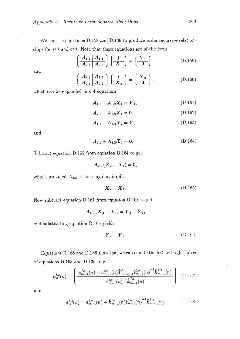
Appendix D. Recursive Least Squares Algorithms 200
We can use equations D.158 and D.136 to produce order recursive relation-
ships for ei'q and cJ'q. Note that these equations are of the form
lffil t+l :[+) (D15e)
and (ffi] t+l :[+] , (D160)
which can be expanded into 4 equations
At,t * At2Xt-Yr,, (D.161)
Az¡ * A2,2X1:O, (D.162)
Ar,r * At,zXz - Y2 (D.163)
and
Art]-Ao.rXr:O (D.164)
Subtract equation D.162 from equation D.164 to get
Ar,r(Xz - Xr) :0,
which, provided A2,2 is non-singular, implies
Xz: Xt' (D.165)
Now subtract equation D.161 from equation D.163 to get
Ar,z(Xz-Xr) -Yz-Yt,and substituting equation D.165 yields
Yz:Yt. (D.166)
Equations D.165 and D.166 show that we can equate the left and right halves
of equations D.158 and D.136 to get
"k,@):í I ,o ,u1l.Jand
,rÅo@) : er;n_rçr¡ - fr::_r@)e!_r(n)-t îr2o_,,("). (D.168)
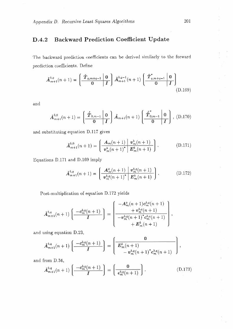
Appendix D. Recursive Least Squares Algorithms 201
D.4.2 Backward Prediction Coefficient Update
The backward prediction coefÊcients can be derived similarly to the forward
prediction coefficients. Define
and
and using equation D.23,
and from D.34,
Ã!]*rç" + r)
Ãu,,]*r("+ 1) :
Ã!iÎ*,(n * 1) : TO,m-l 0
à (n+1) Ì|,^*o-, 0b,8-7m17 0
0 I Â^+t(n + 1)
(D.16e)
, (D.170)
(D.171)
(D.r72)
and substituting equation D.117 gives
ÃoiÎ*r(r+1) : I
A^(n -l L) ab^(n + 1)
"b^(" + 1). Eb^(n + t)
Equations D.171 and D.169 imply
Ãu,,|*r(n * 1) : Al"(n + I) ab;ß(n + l)
"b;f (" + 1). Eb^(n + t)
Post-multiplication of equation D.I72 yields
Ã!]*r(" + t¡-A!.,("+l)c[q(n+1)
+ abff(n + L)
-ab,;l("*1).cþq(n*1)+ Eb^(n + 1,)
Eb*(n + t)- ab#Ø + l).clq(n + 1)
0
Ã!j*rç" + r)
(D.173)
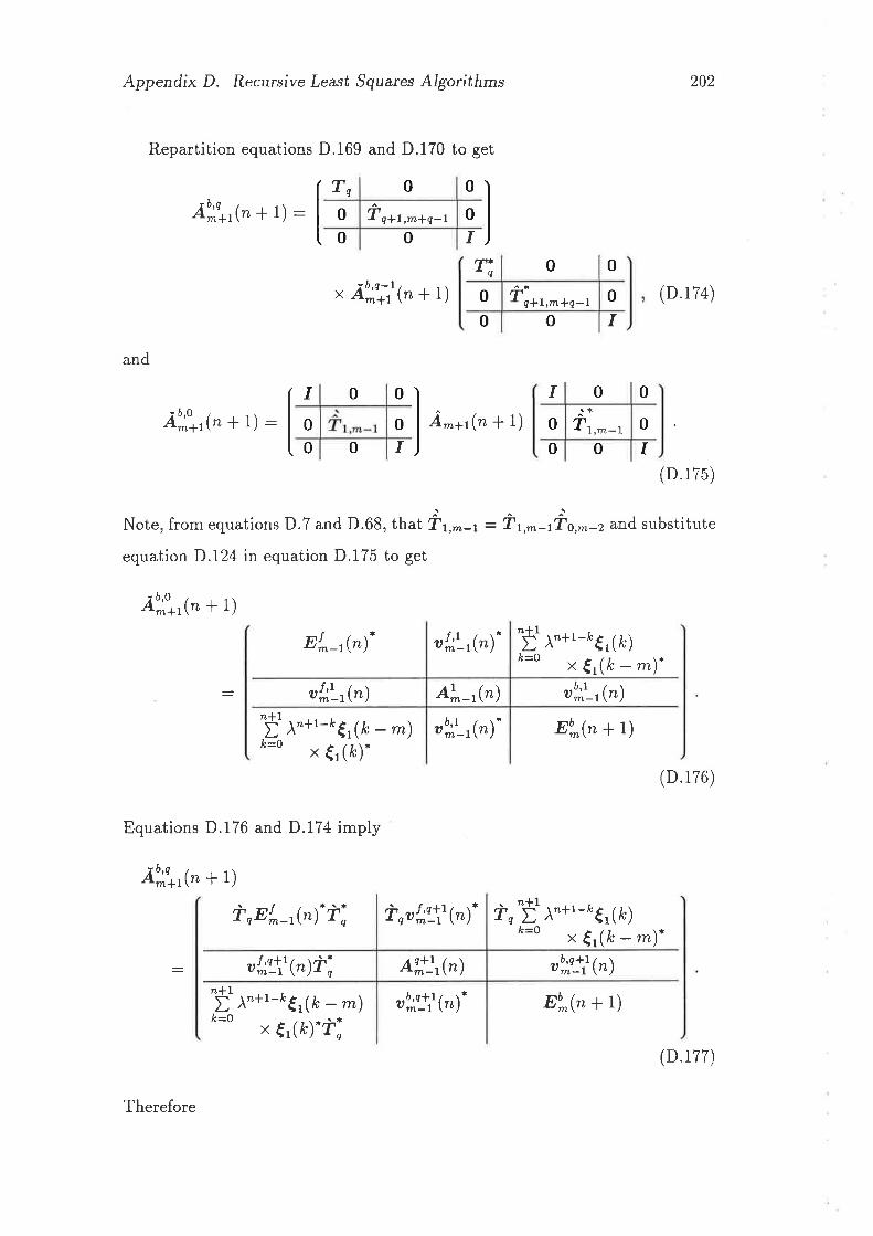
Appendix D. Recursive Least Squares Algorithms
Repartition equations D.169 and D.170 to get
202
0
0 (D.174)
Ã!if*,(n * 1) : 0I
o
0
x À|'*-i 1" + r1
r;00
I 0 0
A^*r(n + t)
Ãu,,|*t(n * 1) :0
0I
qT00
and
00 0
,rÅ'-r(")
0
0 I
I 0
00 0
(D.175)
0
0
I
Note, from equations D.7 and D.68, that fr,-- t : Ìt,^-tùo,*-, and substitute
equation D.I24 in equation D.175 to get
-À nAî+r(n + 1)
Et^-r(")-n*l5'&=0
À"+1-e€1(k)x €r(fr - *)*"bi,]-,,(")
ok'-r(r).
"f ¡"*t-o €,r(k - *)'b=o x €r(k).oui]-r(n)- nb^@ + t)
Equations D.176 and D.174 imply
Ã!,,]*r(n + 1)
ùrEr^-r(").i, i'oar;\tç"¡-
"t;\'ç"¡ù,n*lD
/c=0
"u,ifjÌ (")
).
. n*1TnD/c=O
)"+t-fr€r(k)x €r(k - *)*
(D.176)
l"+1-À€1(k _ m)x {r(k).T,
T q¡t,rn¡q-t
ùi*r,^*o-,
Irrn-1T
A'*-r(")
A1,I]rØ)
Therefore
ou,ifjrt(" Eb^(n + t)
(D.177)
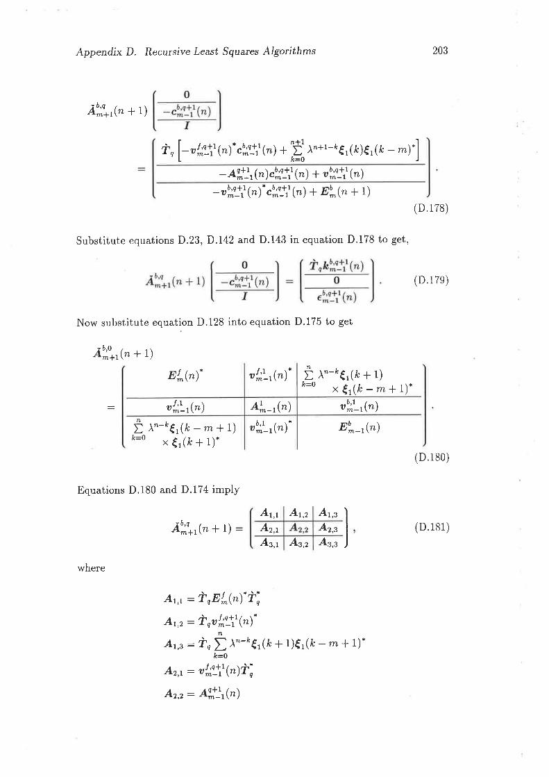
Appendix D. Recursive Least Squares Algorithms 203
Ã!]*r(" + t¡
-o*\'(,,)."l;o-*i(") + Ët À"+1-e€1(k)€,r(k - *)È-o
- A'::r(") cb,iflrL (") + ab#:| (n)
-"!!r'(")- "u#:l (") + nb^@ + t)
Substitute equations D.23,D.L42 and D.143 in equation D.178 to get,
ù q
Now substitute equation D.128 into equation D.175 to get
Ã!,il*r(n + 1)
(D.178)
(D.17e)
(D.180)
(D.181)
ør^(")-
ok'-r(r)
É l"-o€r(fr - rn + 1)fr=o x€r(fr+1).
Ë r"-*€r(k+ 1)k=o x€r(k -**I).or^t-r(n).
ooÅt-r(")
ou,;t-r(n)* Eu^-t(")
Equations D.180 and D.174 imply
where
At,t A,oÃ!,,|*r(n * 1) : Az,t Ar,"
As,t As,z
AtJ : i'rnj^@).ùi
At,z: i'nol;\t1"¡-n
Atp :i' t À"-߀1(fr + 1)€1(k - * * L)*È=O
A2J: "r;\'(")A2,r: A*]r(")
At,s
Az,s
ù;
At*-t(")
Appendix D, Recursive Least Squares Algorithms 204
Az,z: "b¡!rt(")nAzr : D l"-o€,( lc - m+ 1)€r(t + t).r,
È=0
As,z: "u,;fjl(").Ar,, : Eu^-t(").
Therefore
Ãb]*r(" + t)
and
ù,lnt^ç"¡. - ,rÅ\t (")- "k\'(")lù;l" k\' Ø) - All],Ø¡ ct;\' ç"¡) ùii
^-rË^(k - *+ 1)€,(k + r).À=o
-"u,iijiØ). crÅ\'@)lù;
Substitute equations D.23, D.149 and D.150 in equation D.182 to get
(D.182)
(D.183)
(D.184)
(D.185)
(D.186)
In order to manipulate equations D.179 and D.183 more easily define
è|'jr' @) : ù' o rk\' @)ùi,a2'!,'@) : ki;\t(fiù|
Ã';,|*r(n + 1)
î,'J!l r"l : ù nrcbfll (n)
Using equations D.184, D.185 and D.186, rewrite equation D.179
0
,',iiji @)
Ã!j*r1" + t¡ (D.187)
Appendix D. Recursive Least,Squares Algorithms
and rewrite equation D.183,
205
(D.188)Ã!,,|*r(n + 1) 0
^ /'q+1
k*-t (r)
Multiply equation D.188 ay èr;\'çrf'î::::(n) ro ger
è1\',@)-'ã!]iiø¡
- "r;\' (,)ùièr;\' ç"¡-' ãlill r"¡Ãu,,]*r(n + 1)
ab;o*rç" + t¡
I å'q*1k^-t (n)
I
0
and subtract equation D.189 from equation D.187 to get
ã*' l,' @¡ ¿';:-i' r " I -'
â ]'-T t " I
:Í,q|l, ' -1 î å'c+t .
-e*'-l (") k^_, (r)
-"b¡!r'çr¡ + cr;\'(n)ùièr;'!r' çr¡-' îl]ii f"¡
(D.18e)
I00
(D.1e0)
Equations D.190 and D.173 are of similar form to equations D.158 and D.136
and we can equate the left and right hand sides of equations D.190 and D.173
to yield two new equations,
,):[] IJ(D.1e1)
,o,iiji @) - î:':,' ç,¡ê!;'!,'çnf'îliii f"¡
and
el,f (,+ 1) : ,bf!,'çn¡ -ã!^'1,'Ø)ê:i*,'(")-'î'!iiiro. (D.re2)
Appendix D. Recursive Least Squares Algorithms 206
Equations D.167 and D.191 are order update equations for the forward and
backward predictor coefficients. Equations D.192 and D.168 are used to update
¿f ,o ¿¡¡[ 6b,t.
D.5 Error Update
Using equations D.1, D.12, D.3 and D.5,
( *i"_,(n * 1) _l (D. re3)at^(n+1) :tmJ .
Pre-multiply equation D.167 by equation D.193 to get
æ7^(n + 1)" ct;q (n) : æ!^-r(n * I). cr;n-r(r)
- lr\^-r(n + l)- cb,if-r(r) - d'b^-r(n + t')l
* ùi ¡ o _, eb¡ -, çr¡-' fr,20-, (n),
and from equation D.I4,
æk@ + L). cr;q (n) : *L-,,(n * I)- cr;1t (")
+ eb,if _t@ + 1 ). i;+q _rè,,il_r@)-t îr2o_,,(r),
and applying equation D.14 again,
dr*("+ 1)- - ekn(n+ 1). : d*-t(r+ 1). - e^a(n ! I)*
+ eb,if _ Jn + 1 )
. i; + q _, è0,^t _, çr¡- t
fui;n _, qr¡,
(D.1e4)
anð, d,l^(n + i) : dl^-t(" * 1) from equation D.!2,
ekn(n+ 1). = "Í;o-r(r+ 1). - .b,ll-r(n+ 1).";+q -rèo,il-r(r)-'îtlo-,,(r)(D.1e5)
Similarly, use equations D.1, D.I2, D.3 and D.5 get
æL(" +2) : (D.1e6)
Appendix D. Recursive Least,Squares Algorithms
and pre-multiply equation D.191 by equation D.196 to get
æl^(" *2).cbf (n + 1) : *flr("+ t).clo-+rl(n)
- lr'Ì]r(n + t)" cr;l*rt(r) - dr^-r(" 1 l).J
* ùièl'J,' @)-' îo::: @),
and applying equation D.14 we get
du^(" +z). - eb.,f (" +2)- : dþ^-r(n * 1). - "'#:i(n * 1).
+ er;\t (n + t)- ù;èr;'1'qr¡-' îojli çr¡,
and since do^(" +2) : do^-r(" * 1) (from equation D.12),
eb^,f (" + 2)* : .o,iiji@ + 1).
"k\'Ø + tf ù;èr;1*,'(,,)-1 : ö'q*1
.
lc-.--, (r)
207
(D.1e7)
D.6 Auxiliary Variables Update
We have introduced the Auxiliary variables kb'q, k/'ø, which can be used to
calculate the other quantities, but have no particular physical significance. We
need to derive some relationships which will allow these variables to be efficiently
calculated.
Take the conjugate-transpose of equation D.45 and substitute in equation
D.148,
n*7tt-n-,,("): t ¡n+r-ftgr(ß--)€r(k). - Àab,i!-r(n-t)-"r,io-r(n - 1)
&=1
+ [1 - 'y^-r(n)]"b¡-tç"¡"r;'-r(r). - du^-r(")dr^-r(")-
^ (å À'-å€,(k - *)€,r(k)* - ou,;l-r(n - l.cd;1,(r, - 1))
+ {r(, + 1 - m)€Jn+ 1). + lr -''t^-r(n)) eb;q-t(n).f,,;'-r(")-
- d'^-r(")dr^-r(").
Appendix D. Recursive Least Squares Algorithms 208
: ^tckq_t
(" - 1) + [1 - tk-r@)].b¡-r1"¡.t;o_,,(r)*
+ €r(n + 1 - *)Ër(n+ 1). - ab^-rçn¡ar^-r(r).,
and from equation D.12,
ttko_r("): ^teiÅo-t("
- 1) + [1 - tl^_r@)l"b¡_rç"¡ut;n-r(r)*
+ €r(n + 1 - *)€,r("+ 1). - {,(" + 1 - *)€'("+ i).:
^kÍÅc-1(" - 1) + [1 - tl,-r(n)]"b;-rç"¡"t;lr(r).. (D.19s)
Equation D.198 is the recursive form we require for lcf'q.
We will now show that lcb] is the conjugate transpose oI lcr;q. Taking the
conjugate-transpose of equation D.148,n*L
kko_r(n). : D l"+1-Å€1 (k)€, (k - n'r)* - ckq-rØ)- ob,il-r(r),/c=1
applying equation D.23,n*'l
kko_r(n).: Ð ¡n+r-È6,(k)€r(fr -*)* - cko-r("). Al*-r(n)cb{-r(n),Ie=l
and since A is Hermitian,r¿*1
k-o-r(n). : t À"+1 - È €r ( k ) €, ( k - *)* - loL -r@).r^n-r( " )]
. clo-, 1 " ;,È=1
and applying equation D.23 again,n*l
t i;o_r(r). : D À"+1-À€1(k)€,(k - *)* - oko-r(n)- cbf-r(n),fr=1
and comparing with equation D.I42
kr,:o-r(r). - tcb¡-r(n) (D.199)
D.7 Kalman Gain Update
We now proceed to find recursive relationships for the Kalman gain. Substi-
tuting equations D.117 and D.68 in equation D.114 and replacing n * 1 with n
gives
Am+7(,):[,¿-t"l l."Lt"li-- l, (D.200)- | i'^"u*("). | ù^Eu^@)ùi^ )'
Appendix D. Recu¡sive Least Squares Algodthms
and applying equations D.7, D.129 and D.130 gives
209
(D.201)AL*r(t) :
Post-multiplication of equation D.201 gives
and using equation D.23 gives
-Ai@)cbf @)ùi*,+ ab¡@)ùi*,
-ab¡ (r). c!,ii @)ùi*,+ ù^+oÐb^@)ùi*n
ù*+qlnu^@)
- ab¡(n)- co,lT@)lùi*,
0
i'^,rreb¡(n)ùi*,
Al"+r(")
Al"+t(")
and from D.34,
Al"*r(")
and by post-multiplication
Ao**t(")
0
0¿o,ii Ø)
(D.202)
èbj (fi-L ù ^*, lau^ç") - o"li Ø)- gL@)l
0
ù^*olot*f"¡ - ,b,;f (n)- sil(")](D.203)
Substitute equation D.38 in the left hand side of equation D.203 and apply
equation D.15 to get
Al,+,ç,¡ f -.'* (ùùi*,
] .0,,,-' ù
^*néu,# @)
ù ^ +n loP* t"l - ub;ry (n)" sl^(n)
0
(D.204)
Appendix D. Recursive Least Squares Algoilthms
From equations D.201 and D.38
210
(D.205)Al"*t(")
Add equations D.205 and D.204
AL*t(r)0
Ao^+t(r) :
Therefore,
èbf (n)-1ù^+qéb,;:(n)+sl"@)
gn^+r(,): + èbj (n)-r ù **oéo,if @). (D.207)
Similarly, substituting equations D.120 and D.68 in equation D.114 and
replacing n+l with n gives
Am+t (r) : . I . \*Ìr,*îtr^1, - t) I Ìt,*Â.*(n-t)Ìr,^
(D.208)Er^(n - t) ûr^(n- r).âr,-
Note that Ìr,* : Ìr,*ùo,^-1 and apply equations D.129 and D.130
t4ùlComparing equation D.206 with equation D.38 we obtain
: æn^+t(n)(D.206)
(D.20e)
(D.210)
ùnnr^@ - 1)i;- ùnulo+t(n - I). ct;r+11n - 1)Èo
to+l(n _ 1)";- A*t(n - L)ct;q+l(n - 1)?o
Ao^*r(n):
Equations D.209 and D.129 and D.130 imply
AI"+t(")a
Appendix D. Recursive Least Squares Algorithms
and using equations D.23, D.17 and D.184,
21r
(D.211)AL*t(")
and by post-multiplication,
lffil :[+]Al"+t(") êlo*'1, - r¡ -1ù q
x lar*@ - t) - ur;a+r(n - I)- g*'(" - r)J
ùolat,o+rçn - 1) - ohø+t(n - L). gîlt(" - r)]0
(D.2r2)
Substitute equation D.38 in the left hand side of equationD'272 and apply
equation D.15 to get
Al"*t(n)_cr¿,@)ù)*o
e}o ç"¡-t ù ^*oéko (r)I
0
l.2
Tmtq ¿r;n (") - a hø (n)- sl"@](D 3i
From equations D.210 and D.38
Al"*r(")
Add equations D.214 and D.213
.(D.2r4)
At^*,(")([nl-dT lI
+ _¿Lort (n _ 1)Ì; ] ,*'*',, - t¡-'ùoeå'r' - t))
(D.215)
Appendix D. Recursive Least Squarcs Algorithms
Comparing equation D.2I5 with equation D.38 we obtain
272
g?.+Jr):lI
_"tu+r(n _ t)i;(D.216)
D.8 Gamma Update
From equations D.44 and D.38
li"("): æl(n)*g'^("). (D.217)
Substitute equations D.207 and D.193 into equationD.277 to get
ú(") : æq*rgl^-, (") + læ1,-rcb,¡l-, (") - du^*o-r*)
x ùi * reb¡ -, (n)-' ù,* * n -, ëb,ll-, (n),
and substitute equations D.217 and D.15 to get
ú^ (") : 1ï^ _ t( " ) + eb¡ _, qn)- ùi * o _ rèo,il-, (r)- t ù * * n -, é0,;l -, (")
(D.218)
Similarly, substitute equations D.216 and D.196 into equationD.2LT to get
tl^Ø): æll]r.gl.,+.]r(, -Ð +ldr^_l(r - 1). - æf]r(" - r)*chø+t(" - r)]
* ùièr;'*t1, - t¡-'r nêr;ø@ - t),and substitute equations D.217 and D.15 to get
É^(n) : ^Ëllt(, - 1) + ér;\L (n- l)-i;êlil'(r, - r)-' ù nék\' @ - t)
+ ¿20*t (, - r)-t ùoëkn(, - t)
(D.21e)
Appendix D. Recursive Least Squares Algoúthms 2t3
D.9 The Generalized Fast Kalman Algorithm
We now have the recursive relationships we need for a fast Kalman filter. This
section will chiefly consist of organizing the work of previous sections into a
suitable order.
From equations D.12 and D.14
ekn (n - 1) : €i (") - cko (" - 2). æ1,(n - r) (D.220)
From equations D.37 and D.38
cr.,;o (n- 1) : ckn (n - 2) + sl^(n - \efie (n- 1). (D.22t)
Put
f , (") : [1 - oLØ - r). go^(" - \] et;t (n - t). (D.222)
Substitute equation D.217 in equationD.222 and then substitute into equation
D.47 to get
eko(" - 1) : )cr;a@ - 2) + fq(n)er;q(n - 1).. (D.22J)
Substitute equation D.184 into equation D.216 to get
lùorr,o*'(,, - 1)r;] -' ù0e2,çn - r¡
go^+t(r): gl:r@- 1) - ¿tt+r(n - 1)f;x lùoer;n+'(, - 1)à;]-'x Ùoet;oç" - t¡
(D.224)
Re-partition equation D.224 and put
s(")tr(")
: gl"+t@). (D.225)
From equations D.12 and D.14
.u'o (r) : €*(, - t) - cb,;, (n - L)- æl^(n). (D.226)
Appendix D. Recursive Least Squares Algorithms
p(r) - eb¡ çn¡-' ù ^*néo;l
(r)
0 @) : sl^(") - cb¡ ç"¡ùi*o¿u,;: (")-'x ù**oeb¡çr¡
: sl^(") - ebf (eùi.+rttØ).
Use equati on D.229 to substitute for gl"(") in equation D.227
cb,f @): cbj(n- 1) + [of"l - cb¡1"¡ùi*,u@)]eb.,:(,)-,
and collect all terms in cbff(n) as follows
"',if @) [r + ii*, ¡,r(n)ebf (n)-]: .o¡ç" - 1) + þ(n)ebff(n)-.
Therefore
21.4
From equations D.37 and D.38
"b,;f (") : cb¡(n - 1) + sI^@)eb#(n). (D.227)
Unfortunately, we haven't calculated g(n) yet, and we can't simply change the
order of the calculations as we would like to use cfq(n) to calculate g(n). So
we need to be a little devious. Equate equations D.207 and D.225 to get
(D.228)
(D.22e)
.!,f (r): lcb¡çn- 1) + s(n)eb#(nl-] [r +ù-^*ot"(r¡.b¡çr¡.]-' (D.230)
From equation D.229
gl,(") : g(n) + cbff (n)ùi+ouØ) (D.231)
The equalizer calculations are now simple. From equation D.11
yi@):ci(n-1).æ(n), (D.232)
and from equation D.13
eI: di@) - a"^("), (D.233)
and finally, from equations D.37 and D.38,
.i@): ci(n - t) + s^(n)e^(n)* (D.234)
Appendix D. Recursive Least Squares Algorithms 2t5
The algorithm consists of equations D.220, D.221, D.222, D.223, D.224,
D.225,, D.226, D.230, D.231, D.232, D.233 and D.234. We only need the re-
sults for q : 0, but unfortunately, the calculation of g?-+t(") in equation
D.224 requires gt^(" - 1), which in turn requires g'^-r(" - 2) and so on.
In general, therefore, we need to maintain filters with values of rn and q of
(L,*t - I),(2,mt - L),(3, -t - 2) . . .(*t,0) in order for the final filter to have
Ç : 0 and rn - rn1. The equalizer equations (D.232, D.233 and D'234) can be
omitted for all except the final filter.
In general this makes the number of calculations increase as O(rnl) since
we have rn1 filters whose length is proportional to rn1. However, savings are
possible if gl, : gllt at any point. In particular, this happens in the linear
case for g : 0 and so the number of operations in the linear case increases as
o(*).
D.1-0 The Generalized LS Lattice Filter
The Lattice Filter is fundamentally order recursive instead of time recurslve.
As each sample is processed, the filter is reset to zero length and it is then
recursively "grownt' to the desired length.
For each n initialize to m:0. From equation D'11
yi'q(n) :0, s e {e,f ,b},
and from equation D.44
7f;(n) : o,
and from equations D.13 and D.l1 and D.12
e3(") : d,"(n),
and from equations D.13 and D.11 and D.12
eio'o(n - 1) : ¿uo'o("): ebo'n1n¡: €r(n)
(D.235)
(D.236)
(D.237)
(D.238)
Appendix D. Recu¡sive Least Squarcs Algorithms 2t6
From equations D.47, D.236 and D.238
elo,o (n - i) : Àelo,o (n - z) + €r(r)€r.. (D.23e)
Similarly
.å'n(r) : Àebo,q (n- 1) + €r(r)€r. (D.240)
Since equation D.240 is of the same as equation D.239
ebo"Ø):efo'oç'-t)' (D.24r)
Substitute equation D.43 in equation D.198 and replace n with n - 1 to get
t ko_r(n - 1) : Àt iÅo_r(" - 2) + ëo,il_r(n - r)er;q_,(, - 1).. (D.242)
Put
Kkn(r) : îrln-r(n - r)- êu,if-r1n - t¡-1i m*q-L
and substitute equations D.153 and D.152 to get
xkn(") : kr;ø_r(n - r).ùi*o_, (i-*n- ,eb,ll-r(n - Ðù;+c_1)-t ù^+q-r.
(D.243)
Put
xu,if Ø) : ã':::Ø - Ð è:oi,'@- 1)-'rand substitute equations D.186 and D.184 to get
rcu,iiØ) : ku,ifjl("- 1)."; (ùnrt;\'("- 1)r;)-'ùr,and applying equation D.199,
xu,if @) : kr;\l(n- 1)i; (ùorr;\'("- 1)f;)-'ù0.(D.244)
From equation D.243 and equation D.195
q,
eko(n-1) : eko_,,(r-1) - xko("-t)ebf_r(n-t) (D.245)
Appendix D, Recursive Least Squares Algorithms
From equation D.244 and equation D.197
.u,;f (") : eb]!r'(n - 1) - I<o,iiØ - Ð.k\'(" - 1).
From equations D.168, D.153, D.154 and D.152
eko(r- 1) : ,rÅo-,.(, - 1) - lrt;'-r(n - 1).ii,1n-r
x (i-+o-r rb,i!-r(, - t)fi"ao-,
x Ù^+q-tter;q-tçn - t¡,
2r7
(D.246)
-1
and from equation D,243
eko(n-1) : eko-r(r-1) - xt;'çn¡tcr;1'("-1)(D.247)
From equations D.L92, D.185, D.186 and D.184
,0,;f ("): ebljl(n - 1) - kr;\'(" - 1)à;
" (ùrrr;\'(, - 1)";)-'x ùottb;!l(, - 1),
and from equation D.244
eu.,:("): ,o#jrt(" - 1) - Kbj(n)klo-*rt1, - t¡,
and applying equation D.199
,b# Ø) : eb]ll (n- 1) - x6ù¡et;\'(', - 1).'
(D.248)
We copy equation D.105 here for convenience;
vi1n) : u,--t(r,) + z^(n - t¡. [i--,e u^-r(r- 1)r;-,]-' 'Ì^-r.'^-'(')'
(D.24e)
From equaiion D.13
eï: diØ) - vi(")From equation D.43 with t : b,
(D.250)
ë',ll-r(n). : [1 - ^,¿,-r(")].o,il-r(r)- . (D.251)
Appendix D. Recursive Least Squares Algoúthms 218
From equation D.218
t- @) : .tl* - t( ", ) + eb¡ - r (n). ùi + o -r eb¡ - r 1"¡-' ù m * q - L éo,il - r @),
and substituting equation D.L52
ú^(") : -,t1,-t(") + ebff-r(n)- i'i+o -,
" [È-*o-r ru#_r@)ùi*o-, ] -'
x ù^¡o_téu,ii_r@).(D.252)
Finally substitute equation D.43 into equation D.107
,^(r) - Àz*(n - 1) + ù^-rebf-r(n)e;-r(r).. (D.253)
The lattice algorithm consists initializing at each n to m - 0 using equations
D.235, D.236, D.237, D.238, D.239 and D.241. Then equations D.242,D.243,
D.243,, D.244, D.245, D.246, D.247, D.248, D.249, D.250, D.25L, D.252 and
D.253 are repeated ml times with successively increasing rn. Equations D.249,
D.250 and D.253 are only required if an equalizer is being implemented. As
for the case of the Fast Kalman algorithm, we only need results for Ç : 0 but
because equations D.248 D.246 and D.244 are in terms of parameters of the
filter q { 1, we must, in general, maintain filters with values of rn and q of
(L,mt - L),(2,Tn1- l), (3, TTty -2) . . .(*t,0) in order for the final filter to have
q -- 0 and r¿ == Írtrr. The process is illustrated in figure D.4
In general this makes the number of calculations increase as O(rnl) since
we have rn1 filters whose length is proportional to rn1. Howevet, savings are
possible iÎ æ1, : ællr at any point, in which ç¿5s ¿ö'c*1 : ¿b'Q ' In particular,
this happens in the linear case for Ç : 0 when the filter takes on the form of
figure D.3 and the number of operations increases as O(*).
If. Ti : I lor i ) i1, then the computational burden increases as O(i1m)
for rn ) ir. Let us consider a concrete example. In the following discussion,
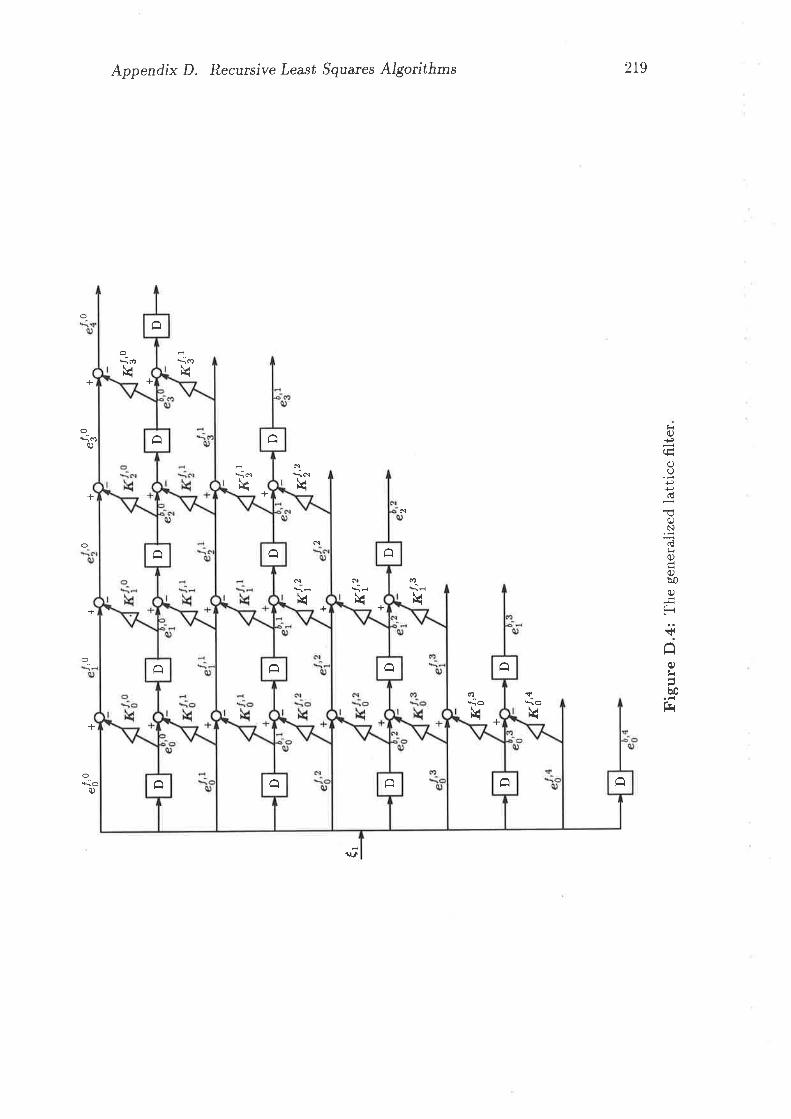
D
DD
D DD
tK
+
l2 I
D DDD
DD DD D"lo'o
,00
.['o
,0+
++
+
K[,0
è ìJ \3 o a- X o o F! ûr o fr o S)
(D C'f € Þ ! o <D Þ O
c o B (n
+
r{{''
Kt'
+ Kt,,
ê s1K
{,'
I{T''
+
2
+K['"
r{lo
'n
t\9
Figu
re D
.4: T
he g
ener
aliz
ed la
ttice
filte
r
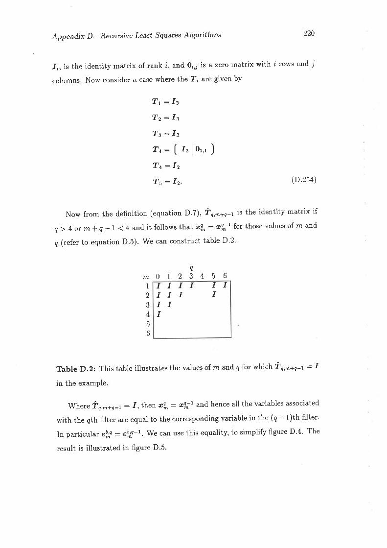
Appendix D. Recursive Least Squares Algoilthms 220
.I; , is the identity matrix of rank i, and o¡,¡ is a zeto matrix with i rows and j
columns. Now consider a case where the T¿ are given by
Tt: Is
Tz: IsTs=IsT¿: ( t, I oz,r )
Tq: Iz
Ts -- Iz (D.254)
Now from the definition (equation D.7), ùr,^¡o-, is the identity matrix if
q > 4 or m ! q -I <4 and it follows lhat æf* - æ?;L for those values of rn and
q (refer to equation D.5). We can construct table D'2'
Table D.2: This table illustrates the values of rn and q for which ùq,^+q-t : Iin the example
Where Û\,^¡n-r: f , then alh: æf;t and hence all the variables associated
with the qth filter are equal to the corresponding variable in the (q - 1)th filter'
In particul ar eb¡ - "o,if-t. We can use this equality, to simplify figure D'4. The
result is iilustrated in figure D.5.
q
n-¿01234561
234b6
II
IIIIIII
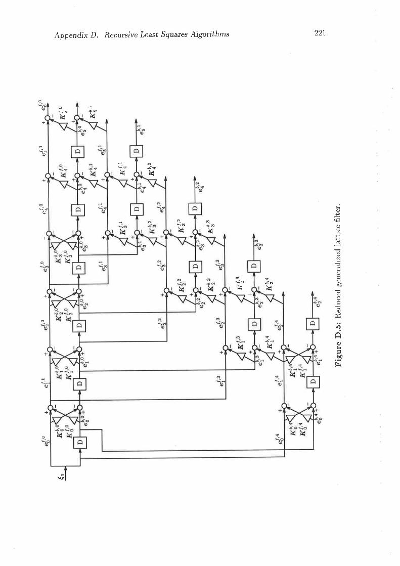
"I,o
"{'o
0,0
00
++
,0+ +
++
+
¿ s1r{
{'o Ku"
't
Þ ìJ ìJ o 5 a- X Þ Þo o ô Ff (D o tr o (â + crì a Þ I o C
D
0q o r.i - + ts C
D
+
Kln
''
K\,,
K[,'
+
I{3ö,
3
Kt'
+
r<0"
'n
f..9 t.,
Figu
re D
.5: R
educ
ed g
ener
aliz
ed la
ttice
filte
r
Bibliography
[1] Oscar Agazzi, David G. Messerschmitt, and David A. Hodges. Nonlinear
echo cancellation of data systems. IEEE Transactions on Communications,
30 (l.I) :2a21 -2 433, 1982,
t2l S. J. Anderson. Simulation and modelling for the Jindalee over-the-horizon
radar. Mathematics and cornputers in simulatúon,27:24I-248, 1985.
[3] D. E. Barrick. FM/CW signals and digital processing. NOAA Technical
Report ERL 283-WPL 26, U.S. Department of Commerce National Oceanic
and Atmospheric Administartion, Boulder, Colarado, July 1973.
[4] E. Bedrosian and S. O. Rice. The output properties of Volterra systems
(nonlinear systems with memory) driven by harmonic and Gaussian inputs'
Proceedings of the IEEE, 59(12):1688-1707, December 1971'
[5] M. Bellafemina and S. Benedetto. Identification of nonlinear channels for
digital transmission. In Proc. ISCAS 85, pages L477-1490, 1985.
[6] Julius S. Bendat. Nonlinear Systern Analysis anil ldentification, chapter
3.4, pages 110-113. John Wiley and Sons, 1990.
[7] Julius S. Bendat. Nonlinear System Analysis and ldentifi,cation. John
Wiley and Sons, 1990.
t8] S. Benedetto, E. Biglieri, and R. Daffara. Modeling and performance evalu-
ation of nonlinear satellite links-a Volterra series approach. IEEE Trans-
actions on Aerospace Electronic systerns, 15(4):494-507, July 1979.
222
Bibliography 223
[9] Sergio Benedetto and Ezio Biglieri. Nonlinear equalization of digital
satellite channels. IEEE Journal on Selected Areas in Cornrnunications,
1(1):57-62, January 1983.
[10] A. L. Berman and C. E. Mahle. Nonlinear phase shift in traveling-wave
tubes as applied to multiple access communication satellites. IEEE Trans-
actions on Cornmunication Technology, 18(1):37-48, February 1970.
[11] Ezio Biglieri, Allen Gersho, Richard D. Gitlin, and Tong Leong Lim.
Adaptive cancellation of nonlinear intersymbol interference for voiceband
data transmission. IEEE Journal on Selected Areas in Communications,
2(5):7 65-777, September 1984.
[12] Nelson M. Blachman. Detectors, bandpass nonlinearities, and their opti-
mization: Inversion of the Chebyshev transform. IEEE Transactions on
Information Technology, 17 (4):398-404, July 1971.
[13] H. S. Black. U.S. Patent 1,686,792, October 1929
[14] H.S. Black. Stabilized feedback amplifiers. The Bell System Technical
Journal, 13:1-18, January 1934.
[15] Boualem Boashash, editor. Proceedings of the lst IASTED International
Symposium on Signal Processing and its Applications, Brisbane, August
1987. IE Aust.
[16] Hendrik W. Bode. Networlc Analysis and Feedbacle Design Robert E.
Kreiger Publishing Company, Huntington, New York, 1975. Original edi-
tion, 1945.
[17] Robert E. Bogner, Ian Dall, and Richard G. Lane. Distortion effects in over
the horizon radar. In Boualem Boashash and Peter Boles, editors, Proceed-
ings of the 1990 IASTED International Symposium on Signal Processing
and its Application.s, pages 391-396, Gold Coast - Australia, August 1990.
Bibliography 224
[18] K. G. Budden. The Propagation of Radio Waues, chapter 13.11-13.12.
Cambridge University Press, 1985.
[19] A. Bruce Carlson. Cornmunication Systems, chapter 4, pages 145-146
McGraw-Hill, New York, second edition, 1975.
[20] Ph Charas and J. D. Rogers. Improvements in on-board TWTA perfor-
mance using amplitude and phase predistortion. In IEE International Con-
ference on Satellite Communication System Technology, pages 270-280,
April 1975.
[21] D.L. Cheadle. Selecting mixers for best intermod performance
crou)o,ues) 12(12):58-62, December 1973.
Mi-
[22] John M. Cioffi and Thomas Kailath. Fast recursive-least-squares transver-
sal filters for adaptive filtering. IEEE Transactions on Acoustics, Speech,
and Signal Processing, 32(2):304-337, April 1984.
[23] Ian W. Dall. Modelling nonlinear distortion in mixers. In R.F. Barrett,
. editor, Proceedings of Australian Symposium on Signal Processing and Ap-
plications, pages 7I8-I22, Adelaide, April 1989. IEEE South Australian
Section.
l24l Ian W. Dall and Robert E. Bogner. Modeling nonlinear communication
systems. In Boashash [15], pages 357-362.
[25] J. J. Dongarra, C. B. Moler, J. R. Bunch, and G. W. Stewart. Linpack
Users' Guide, chapter 9. Siam, Philadelphia, 1979.
[26] J. J. Dongarra, C. B. Moler, J. R. Bunch, and G. W. Stewart. Linpack
Users' Guide, chapter 11. Siam, Philadelphia, 1979.
[27] George Frederick Earl. The influence of receiver cross-modulation on at-
tainable HF radar dynamic range. IEEE Transactions on Instrumentation
and, Measurement, 36(3):776-782, September 1987.
Bibliography 225
[28] D. D. Falconer. Adaptive equalization of channel nonlinearities in
QAM data transmission systems. The Bell System Technical Journal,
57(7):2589-2611, 1978.
[29] L.E. Franks. Signal Theory, chapter 4.4, pages 79-81. Prentice Hall Inc.,
1969.
[30] J. C. Fuenzalida, O. Shimbo, and W. L. Cook. Time domain analysis of
intermodulation effects caused by nonlinear amplifers. COMSAT Technical
Reuiew, 3(1):89-1a1, spring 1973.
[31] Denis Gabor. Communication theory and cybernetics. IRE Transactions
- Circuit Theory, pages 19-31, December 1954.
[32] Denis Gabor, W. P. L. Wilby, and.R. Woodcock. A universal non-linear
filter, predictor and simulator which optimizes itself by a learning process.
The Proceedings of The Institute of Electrical Engineers, pages 422-440,
July 1960.
[33] Allen Gersho and Ezio Biglieri. Adaptive cancellation of channel nonlinear-
ities for data transmission. In P. Dewilde and C. A. May, editors, Linles forthe Future, pages 1239-1242, North Holland, 1984. IEEE, Elsevier Science
Publishers B.V.
[34] Georgios B. Giannakis. Cumulants: A powerful tool in signal processing
Proceedings of the IEEE, 75(9):1333-1334, September 1987.
[35] Georgios B. Giannakis and Jerry M. Mendel. Identification of nonmini-
mum phase systems using higher order statistics. IEEE Transactions on
Acoustics, Speech, and, Signal Processing, 37(3):360*, March 1989.
[36] Henri Girard and Kamilo Feher. A new baseband linearizer for more ef-
ficient utilization of earth station amplifiers used for QPSK transmission.
IEEE Journal on Selected, Areas in Communications,l(1):a6-56, January
1983.
Bibliography 226
[37] P. Hetrakul and D. P. Taylor. Compensators for bandpass nonlinearities
in satellite communications. IEEE Transactions on Aerospace Electronic
Systems, 12(a):509-514, July 1975.
[38] Michael L. Honig and David G. Messerschmitt. Adaptiae Filters: Struc-
tures, Algorithms and Applications. Kluwer, 1984.
[39] Michael L. Honig and David G. Messerschmitt. Adaptiue Filters: Struc-
tures, Algorithms and Applications, chapter 3.1, page 43. Kluwer, 1984.
[a0] Michael L. Honig and David G. Messerschmitt. Adaptiue Filters: Struc-
tures, Algorithms and Applications, chapter4, pages 85-123. Kluwer, 1984.
[41] Michael L. Honig and David G. Messerschmitt. Adaptiue Filters: Struc-
tures, Algorithrns and Applications, chapter 6, pages 144-242. Kluwer,
1984.
[a2] Michael L. Honig and David G. Messerschmitt. Adaptiae Filters: Struc-
tures, Algorithms and Applications, chapter 3.1, page 46. Kluwer, 1984.
[43] E. Imboldi and G. R. Stette. AM-to-PM conversion and intermodulation
in nonlinear devices. Proceed,ings of the IEEE,61(6):796-797, July 1973.
[44] Kyoung Il Kim and Edward J. Powers. A digital method of modeling
quadratically nonlinear systems with a general random input. IEEE Trans-
actions on Acoustics, Speech, and Signal Processing, 36(11):1758-1769,
November 1988.
[45] Young C. Kim and Edward J. Powers. Digital bispectral analysis and its
applications to nonlinear wave interactions. IEEE Transactions on Plasrna
Science, 7 (2):120-131, June 1979.
[46] A. C. Klauder, A. C. Price, S. Darlington, and W. J. Albersheim. The
theory and design of chirp radars. The Bell System Technical Journal,
39(a):7a5-808, July 1960.
Bibliogtaphy 227
[47] Taiho Koh and Edward J. Powers. Second order Volterra filtering and
its application to nonlinear system identification. IEEE Transactions on
Acoustics, Speech, and, Signal Processing, 33(6):1445-1455, December 1985.
[48] Daniel T. L. Lee, Martin Morf, and Benjamin Friedlander. Recursive least
squares ladder estimation algorithms. IEEE Transactions on Acousti,cs,
Speech, and Signal Processing,29(3):627-64L, June 1981.
[a9] Mohammad Maqusi. Analysis and modeling of intermodulation distortion
in wide-band cable TV channels. IEEE Transactions on Communications,
35(5) :568-572, May 1987 .
[50] Robert Aram Minasian. Intermodulation distortion analysis of MESFET
amplifiers using the Volterra series representation. IEEE Transactions on
Microwaue Theory and Techniques,, 28(1):1-8, January 1980.
[51] M. S. Mueller. Least-squares algorithms for adaptive equalizers. The Bell
System Technical Journal, 60(8): 1905-1925, October 1981.
[52] M. S. Mueller. On the rapid initial convergence of least-squares equalizer
. adjustment algorithms. The BeII System Technical Journal,60(10):23a5-
2358, December 1981.
[53] M. Nashed and Robert E. Bogner. Harmonic generation with specified am-
plitude transformation. ,4usúralian Telecommunication Research,20(1):31-
39, December 1985.
[54] Chrysostomos L. Nikias and Mysore R. Raghuveer. Bispectrum estimatton:
A digital signal processing framework. Proceedings of the IEEE,75(7):869-
891, July 1987.
[55] Phillip F. Panter. Communication Systems Design, chapter 7.4.I,7.4.2,
pages 18ti,187. McGraw-Hill, New York, 1972.
[56] Phillip F. Panter. Communication Systems Design,, chapter 7,8, pages 181-
252. McGraw-Hill, New York, 1972.
Bibliography 228
[57] Athanasios Papoulis. Proóability, Random Variables, and Stochastic Pro-
cesses) chapter 5-6, pages 115-120. McGraw-Hill Series in Electrical Engi-
neering. McGraw-Hill, second edition, 1984.
[58] J. A. Richards. Analysis of Periodically Time-Varying Sgstems, chapter
1.2, pages 7-9. Springer-Verlag, 1983.
[59] Ch. P. Ritz, E. J. Powers, and C. K. An. Applications of digital bispectral
analysis to nonlinear wave phenonema. In Boashash [15], pages 352-356.
[60] Enders A. Robinson and Manuel T. Silva. Digital Signal Processing and
Time Series Analysis, page 364. Holden-Day, pilot edition, 1978.
[61] Rob J. Roy and James Sherman. A learning technique for Volterra series
representation. 'IEEE Transactions on Automatic Control, pages 761-764,
December 1967.
[62] A. A. M. Saleh. Frequency-independent and frequency-dependent nonlin-
ear models of TWT amplifiers. IEEE Transactions on Communicat'ions,
29(IL) :L7 L5-L7 20, November 1981.
[63] A. A. M. Saleh. Intermodulation analysis of FDMA satellite systems em-
ploying compensated and uncompensated TWT's. IEEE Transactions on
Communications, 30(5): 1233 -L242, May 1982.
[64] A. A. M. Saleh and J. Salz. Adaptive linearization of power amplifiers in
digital radio systems. The Bell Systern Technical Journal,,62(a):1019-1033,
April 1982.
[65] Gunkicki Satoh and Toshio Mizuno. Impact of a new TWTA linearizer
upon QPSK/TDMA transmission performance. IEEE Journal on Selected
Areas in Comrnunications, 1(1):39-a5, January 1983.
[66] M. Schetzen. The Volterca and Wiener Theories of Nonlinear Systems,
pages I23-L4L Wiley, New York, 1980.
Bibliography 229
[67] M. Schetzen. The Volterra and Wiener Theories of Nonlinear Systems.
Wiley, New York, 1980.
[68] M. Schetzen. Nonlinear system modeling based on the Wiener theory.
Proceedings of the IEEE,69(1):1557-1573, December 1981.
[69] Ronald G. Sea and André G. Vacroux. On the computation of intermod-
ulation products for a power series nonlinearity. Proceedings of the IEEE,
pages 337-338, March 1969.
[70] H. Seidel. A microwave feed-forward experiment. The Bell System Tech-
nical J o urn al, 50 (9) :2879- 1 I 1 6, November 1 97 1 .
[71] H. Seidel, H. R. Beurrier, and A. N. Friedman. Error-controlled high power
linear amplifiers at VHF. The Bell System Technical Journal, a7(5):651-
722, June 1968.
l72l O. Shimbo. Effects of intermodulation, AM-PM conversion and additive
noise in multicarrier TWT systems. Proceedings of the IEEE,59(2):230-
238, February 1971.
[73] G.R. Stette. Calculation of intermodulation from a single carrier ampli-
tude characteristic. IEEE Transactions on Communications, 22(3):319-
323, March 1974.
[74] B. D. H. Tellegen. Interactionbetweenradio waves. Nature,13l(3319):840,
June 1933.
[75] Jitenda K. Tugnait. Comments on "Cumulants: A powerful tool in signal
processing". Proceedings of the IEEE,77(3):a91-492, March 1989.
[76] Ronald E. Walpole and Raymond H. Myers. Probability and, Statistics forEngineers and Scientisús, chapter 5.2, pages 145-148. Macmillan Publish-
ing Co., Inc.,1972.
[77] Bernard Widrow, John M. McCool, Michael G. Larimore, and C. Richard
Johnson, Jr. Stationary and nonstationary learning characteristics of the
Bibliography 230
LMS adaptive filter. Proceedings of the IEEE,,6a(8):1151-1162, August
t976.
[78] Norbet Wiener. Nonlinear Problems in Random Theory, chapter 10,11,
pages 88-100. The Technology Press, M.I.T. and John Wiley and Sons,
Inc, New York, 1958.
[79] Norbet Wiener. Nonlinear Problems in Random Theory. The Technology
Press, M.I.T. and John Wiley and Sons, Inc, New York, 1958.