Signaling in Online Credit Markets∗

Kei Kawai†

New York University

Ken Onishi‡

Northwestern University

Kosuke Uetake§

Yale University

January 2014

Abstract

Recently, a growing empirical literature in industrial organization studies the effect

of adverse selection on market outcomes and welfare. In this paper, we ask the natural

next question, how signaling affects equilibrium outcomes and welfare in markets

with adverse selection. Using data from Prosper.com, an online credit market, we

estimate a model of borrowers and lenders where low reserve interest rates can signal

low default risk. We compare a market with and without signaling relative to the

baseline case with no asymmetric information. We find that adverse selection destroys

16% of total surplus, up to 95% of which can be restored with signaling. We also find

the credit supply curves to be backward-bending for some markets, consistent with the

prediction of Stiglitz and Weiss (1981).

JEL Code: D82, D83, G21, L15

KEYWORDS: Signaling, adverse selection, structural estimation

1 Introduction

Inefficiencies arising from adverse selection is a key feature in many markets, with exam-

ples ranging from “lemons” in used car markets (Akerlof, 1970) to toxic assets in financial

∗We thank Igal Hendel, Hide Ichimura, Alessandro Lizzeri, Aviv Nevo, Isabelle Perrigne, Rob Porter,

Jeffery Prince, Quang Vuong, Yasutora Watanabe, and Michael Whinston for their valuable comments and

suggestions.†New York University Stern School of Business: kkawai@stern.nyu.edu.‡Northwesern University: onishi@u.northwestern.edu§Department of Marketing, Yale School of Management: kosuke.uetake@yale.edu

1

markets (Morris and Shin, 2012). An important source of inefficiency in these markets lies

in the inability of agents who are of “good” types (e.g., sellers of high–quality cars) to dis-

tinguish themselves from the “bad” (e.g., sellers of low–quality cars), resulting in markets

to unravel completely in the worst–case scenario. The key insight of Spence (1973), how-

ever, is that when costly signaling devices are available, agents who have different marginal

cost of signaling can be induced to take action that reveals their true type in equilibrium.

Hence signaling can prevent the market from unraveling, with possibly large welfare im-

plications.

Recently, there is a growing empirical literature in industrial organization that studies

the effect of adverse selection on market outcomes and welfare.1 In this paper, we ask the

natural next question, how signaling affects equilibrium outcomes and welfare in markets

with adverse selection. While the theory of signaling has been applied to a wide range of

topics in industrial organization, there is very little empirical work that quantifies the extent

to which signaling affects market outcomes and welfare relative to a market with no signal-

ing (i.e., pooling). An empirical analysis of welfare seems especially important given that

whether signaling improves or decreases total welfare relative to pooling is theoretically

ambiguous.2

This paper studies these questions by building an estimable model of signaling in credit

markets for unsecured loans using data from Prosper.com, an online peer-to-peer loan mar-

ket. At least since the seminal work of Stiglitz and Weiss (1981), markets for unsecured

loans have been considered to be classic examples of markets that suffer from potential ad-

verse selection problems. A key feature of Prosper.com, however, is that each borrower can

post a public reserve interest rate – the maximum interest rate that the borrower is willing

to accept – when the borrower creates a listing on its Web site. In this paper, we provide

evidence that the borrower’s reserve interest rate signals his creditworthiness and explore

how signaling affects market outcomes and welfare.

While Prosper is a relatively young and small market, it is an ideal setting for inves-

tigating the effect of signaling on market outcomes and welfare. First, in this market we

observe both the reserve interest rate choice of the borrower as well as the contract interest

rate determined by the auction. The contract interest rate is the actual interest rate that the

borrower faces in repayment and it is often lower than the reserve interest rate. Because the

1See Einav, Finkelstein and Levin (2010) for a survey and motivation of recent papers that go beyond

testing the existence of information asymmetry.2For a brief discussion of how signaling equlibriun can be pareto dominated by a pooling equilibrium, see

Mas-Colell, Whinston and Green (1995), Chapter 13.C, p.454.

2

reserve interest rate should not affect the borrower’s repayment behavior conditional on the

contract interest rate, we can isolate the signaling value (as opposed to moral hazard) of the

reserve rate by studying how the reserve rate correlates with the default probability condi-

tional on the contract interest rate. Second, transaction in this market takes place online and

basically all of the information that lenders observe about the borrowers are also available

to the econometrician, unlike in traditional markets. This feature makes us somewhat less

concerned about unobserved heterogeneity than in other settings.

The idea that the reserve interest rates can signal the borrowers’ creditworthiness is

quite intuitive in the particular market we study. Consider, for example, a borrower who

is posting a high reserve rate – say, higher than the prime rate charged for typical bank

loans. Then the lenders may infer that this borrower faces difficulty borrowing from out-

side sources, which also raises concerns about the repayment ability of the borrower. This

will lead lenders to charge a high interest rate to compensate for the high risk. Of course,

this intuition is not a complete explanation of signaling, because there needs to be a coun-

tervailing force that induces the borrower to post a higher reserve interest rate. In the market

we study, the natural countervailing force is the probability of obtaining a loan. As long as

the funding probability increases as a function of the reserve rate, this can counteract the

incentive for the borrower to post a low reserve rate. These two opposing incentives cre-

ate different trade-offs for different borrowers, giving rise to the possibility of equilibrium

dispersion in the reserve rate.

This rather simple intuition forms the basis of our model of the borrowers. In our

model, borrowers are heterogeneous with regard to the cost of borrowing from outside

sources and the ability to repay the loan. Given a trade-off between higher funding prob-

ability and higher interest rate, the heterogeneity in the cost of borrowing translates to the

single-crossing condition. The low-cost types (e.g., borrowers with easy access to credit

from local banks) value a decrease in the interest rate on the potential loan relatively more

than an increase in the probability of obtaining a loan from Prosper. Conversely, the high–

cost types (e.g., borrowers that do not have access to outside credit) would value an increase

in the probability of obtaining a loan relatively more than a decrease in the interest rate.

As long as the low–cost types also tend to have higher ability to pay back loans, a sep-

arating equilibrium can be sustained in which the low–cost types have incentives to post

low reserve rates (and receive low interest loans with relatively low probability) and the

high–cost types have incentives to post high reserve rates (and receive high–interest loans

with relatively high probability).

3

In order to see whether the reserve interest rate functions as a signal in this market,

we begin our analysis by providing results from a series of regressions. In our first set of

regressions, we examine the effect of the reserve interest rate on the funding probability

and on the actual interest rate conditional on being funded. The results indicate that a

lower reserve rate leads to a lower funding probability, but it also leads to a more favorable

contract interest rate on average even after controlling for various observables and selection.

This implies that borrowers indeed face a trade-off between the funding probability and the

interest rate in setting the reserve rate. Moreover, this is consistent with the notion that there

exists heterogeneity in how borrowers evaluate this trade-off: The considerable dispersion

that we observe in the reserve interest rate suggests that those who post high reserve rates

care more about the probability of being funded than about what interest they will pay and

vice versa.3

In our second set of regressions, we examine whether there are any systematic differ-

ences between those who post high reserve rates and low reserve rates. We find that those

who post high reserve rates are more likely to default than those who post low reserve rates,

even after conditioning on the contract interest rate (the actual interest rate that the bor-

rower pays on the loans). From the perspective of the lender, this implies that the reserve

interest rate is informative about the creditworthiness of the borrower, i.e., the reserve rate

is a signal of the borrower’s unobserved type.

Given the results of our preliminary analysis, we devote the second part of our paper

to developing and estimating a structural model of the online credit market that agrees

with the basic findings of the preliminary analysis. Our model of the borrowers allows

for heterogeneity regarding creditworthiness and the cost of borrowing, which are privately

known to the borrowers. The borrowers choose which interest rate to post, where the choice

reveals their types in equilibrium. As for the supply side of the credit market, we model

the lenders to be heterogeneous regarding their attitude toward risk. Each lender chooses

whether to fund a listing or not, what interest rate to charge, and how much to lend. Once

the loan is originated, the borrower faces monthly repayment decisions, which we model

as a single–agent dynamic programming problem.

In terms of identification, the key primitives of the model that we wish to identify are

the distribution of the borrowers’ types and the distribution of the lenders’ attitude toward

3Note that it is probably safe to assume that many borrowers are aware of this trade-off: In a prominently

displayed tutorial, Prosper informs the borrowers that setting a higher reserve rate increases the probability

that the loan will be funded.

4

risk. For identifying the borrowers’ type distribution, we exploit variation in the borrower’s

reserve rate and how it is related to the default probability. In particular, we use the fact that

the borrower’s type and the borrower’s reserve rate have a one-to-one mapping in a sepa-

rating equilibrium. This feature is very useful, because it allows us to condition on a par-

ticular quantile of the type distribution by simply conditioning on a quantile of the reserve

rate distribution. Then the observed default probability at each quantile nonparametrically

identifies the borrower’s type distribution. The distribution of the lenders’ attitudes toward

risk is also nonparametrically identified by relating the expected return of listings to their

funding probability.

In our counterfactual experiment, we compare the equilibrium market outcome and

welfare under three alternative market designs – a market with signaling, a market without

signaling (i.e., pooling) and a market with no information asymmetry between borrowers

and lenders. In particular, we simulate the credit supply curve under each of the three

market designs by re-computing the lenders’ and borrowers’ behavior using the estimates

of our structural model. As pointed out by Stiglitz and Weiss (1981), the credit supply

curve in loan markets may be backward bending, or non-monotonic in the interest rate,

because of adverse selection.4 The results of our counterfactual support their prediction:

the credit supply curve becomes more backward bending under pooling when borrowers

cannot signal their type with the reserve interest rate.

With respect to welfare, we find that the cost of adverse selection can be as much

as 16% of the total surplus created under no asymmetric information. We also find that

while signaling restores up to 95% of the difference in the surplus between pooling and no

asymmetric information in some markets, it destroys welfare in others. Our results provide

some empirical evidence regarding when signaling may improve welfare. Signaling seems

to improve welfare most when the degree of adverse selection is sever, while it may destroy

welfare when it is modest.

The empirical findings of this paper directly apply only to the market of Prosper.com

and our model is tailored to the setting in which agents signal through the reserve rate.

However, our basic model and identification strategy can easily be extended to study other

settings in which signaling plays an important role. As long as both the signal and the

ex-post performance are observable, our basic approach can be used to quantify the effect

4Recently, Arnold and Riley (2012) shows that the credit supply curve cannot be globally backward-

bending. For the range of interest rates that we obseve, the estimated credit supply curve seems backward-

bending in our data. This may be because the interest rate is capped at 36% by usary laws in our data.

5

of signaling on market outcomes and welfare.

Related Literature Our paper is related to several strands of the literature. First, our

study is related to the literature on adverse selection in credit markets. Since the seminal

work of Stiglitz and Weiss (1981), there have been many studies testing for adverse selec-

tion in credit markets. Examples include Berger and Udell (1992), Ausubel (1999), Karlan

and Zinman (2009), and Freedman and Jin (2010).5 While testing for adverse selection

is important in its own right and is the first step for further analysis, estimating a model

that explicitly accounts for information asymmetry among the players allows researchers

to answer questions regarding welfare and market design. Our paper goes in this direction.

The second strand of the literature to which our paper is related is the theoretical liter-

ature on signaling. Starting with the seminal work of Spence (1973), signaling has been

applied to a wide range of topics. Even confined to applications in industrial organization,

signaling has been applied to advertising (e.g., Milgrom and Roberts, 1986), entry deter-

rence (e.g., Milgrom and Roberts, 1982), and war of attrition (Hörner and Sahuguet, 2011).

More directly related to our paper, there is also a small theoretical literature on signaling

in auctions, whereby a seller signals her private information through the reserve price (Cai,

Riley and Ye, 2007, and Jullien and Mariotti, 2006, for example).6

In contrast to the large body of theoretical work, however, the empirical industrial orga-

nization literature on signaling is very thin. In fact, this paper is the first structural analysis

of signaling in industrial organization to the best of our knowledge. In a related paper,

Ackerberg (2003) studies a model of advertising in which the results can be interpreted

as signaling. However, the relationship between the signal and the type is modeled in a

reduced form manner. More recently, Kim (2012) studies the econometrics of signaling

games with two types. His paper focuses on identification and estimation, but it does not

include an empirical application.7

5Freedman and Jin (2010) uses data from Prosper.com. Other papers that also use the data include Rigbi

(2011), Ravina (2008), Iyer et al. (2010). In Iyer et al. (2010), the authors examine the lenders’ ability to

infer borrowers’ creditworthiness. They find, among other things, that the reserve interest rate affects the

contract interest rate, and note that signaling can be one interpretation of their finding.6Relatedly, Roberts (2013) shows how the reserve rate can be used to overcome unobserved heterogeneity

in auctions. He studies an environment in which there is informational asymmetry between the players and

the econometrician, but there is no asymmetric information between the sellers and the buyers.7Outside of industrial organization, there are some empirical papers that examine signaling – for example,

papers on the sheepskin effect (e.g., Hungerford and Solon, 1987). However, much of the literature has

tended to focus on testing for the existence of signaling (a few exceptions are Gayle and Golan, 2012, and

Fang, 2006).

6

Our paper is also related to the large empirical literature on screening. In particular,

Adams, Einav and Levin (2009) and Einav, Jenkins and Levin (2012) are two papers that

are closely related to our paper. They consider how an auto insurer can screen borrowers

using the down payment. They show that partly because of adverse selection, the lender’s

expected return on the loan is non-monotone in the loan size. A key feature of our paper

that is different from theirs is that our paper examines signaling while their paper exam-

ines screening. Moreover, our model of credit supply has a large number of heterogenous

lenders while their model has a single lender.

2 Institutional Background and Data

2.1 Institutional Background

Prosper.com is an online peer-to-peer lending Web site that matches borrowers with lenders

and provides loan administrative services for the lenders. Established in 2006, it has be-

come America’s largest peer–to–peer lending marketplace, with more than a million mem-

bers and over $280 million in loans. In this section, we describe how Prosper operates, with

a particular emphasis on the auction mechanism used to allocate funds and to determine the

interest rate.8 For details on other aspects of Prosper, see Freedman and Jin (2010).

The sequence of events occurs according to the following timeline, (1) A borrower posts

a listing, (2) Lenders bid, (3) Funding decision is made, (4) The borrower makes monthly

loan repayments. We explain each step in turn.

1. Borrower posts a listing A potential borrower who is interested in obtaining a

loan through Prosper first creates an account with Prosper, who pulls the applicant’s credit

history from Experian, a third-party credit-scoring agency. As long as the credit score is

above a certain threshold, the borrower can create a listing on Prosper’s web site. Each

listing contains information regarding the amount of loan requested, the reserve interest

rate and the borrower’s characteristics. The characteristics of the borrower that appear in

the listing include credit grade, home-ownership status, debt-to-income ratio, purpose of

the loan, as well as any other additional information (text and pictures) that the borrower

wishes to post. The credit grade, which corresponds to seven distinct credit score bins

8The Online Appendix contains a more detailed description of the institutional background.

7

(AA, A, B, C, D, E, and HR), and home-ownership status are both verified by Prosper.9

Other information, such as debt-to-income ratio and purpose of the loan, is provided by the

borrower without verification by Prosper. Finally, a feature of the listing that is important

for our analysis is the reserve interest rate, which is the maximum interest rate that the

borrower is willing to accept.10 The reserve interest as well as the loan amount are both

variables that the borrower chooses, subject to Prosper’s conditions and usury laws.

2. Lenders Bid Prosper maintains a list of active listings on its Web site for potential

lenders. If a potential lender finds a listing to which she wishes to lend money, she may

then submit a bid on the listing, similar to a proxy bid in online auctions. Each bid consists

of an amount that the lender is willing to lend (typically a small fraction of the loan amount

that the borrower requests), and a minimum interest rate that the lender is willing to accept.

The lender can submit a bid with an amount anywhere between $50 and the borrower’s

requested amount, but the modal bid amount is $50. The lender can bid on any active

listing at any time.

For each active listing, Prosper displays the fraction of the loan funded and the active

interest rate in addition to information regarding borrower characteristics, loan amount, and

the reserve interest rate. The active interest rate corresponds to the standing marginal bid

in multi-unit auctions. We will explain what the active interest is, in more detail below.

3. Funding Decision The auction used in Prosper is similar to a uniform–price auc-

tion with a public reserve price. Using an example, we explain below how the terms of the

loan are determined and which lenders end up lending. Suppose a borrower creates a listing

with a requested amount of $10,000 and a reserve interest rate of 25%. Then, Prosper adds

the listing to the set of currently active listings. For simplicity, let us assume that the lenders

can submit a bid amount of only $50. At the time the lender submits her bid, she observes

the fraction of the loan funded and the reserve interest rate. For listings that have yet to

attract enough bids to reach the requested amount (i.e., less than 200 bids in this example;

see left panel of Figure 1) that is all she observes. In particular, she does not observe the

interest rate of each bid. As for listings that have already received enough bids to cover the

9A credit grade of AA corresponds to a credit score of 760+, a grade of A corresponds to 720–759, B to

680–719, C to 640–679, D to 600–639, E to 540–599, and HR to 540–. The numerical credit score is not

listed.10In a tutorial that walks borrowers through the listing process, Prosper advises borrowers to “Think of the

interest your are paying on your next best alternative” when posting the reserve insterst rate.

8

Figure 1: Funding Decision – The figure shows how a loan is funded for the simple case in which lenders

only submit a bid with an amount of $50. The horizontal axis corresponds to amount and the vertical axis

corresponds to the interest rate. The left panel illustrates a situation in which the requested amount is $10,000,

and the listing has received 160 bids ($8,000). The right panel illustrates the situation in which the requested

amount is $10,000, and it has attracted more than 200 bids.

requested amount, (i.e., more than 200 bids, see right panel of Figure 1) the lender observes

the active interest rate, which is the interest rate of the marginal bid that brings the supply

of money over the requested amount. In our example, this corresponds to the interest rate

of the 200th bid when we order the submitted bids according to their interest rate, from

the lowest to the highest (As a matter of terminology, the active interest rate is understood

to equal the reserve interest rate for listings that have not been fully funded). Moreover,

for fully funded listings that are still active, the lender also observes the interest rate of the

losing bids, i.e., the interest rate of the 201st bid, 202nd bid, and so on. However, the lender

does not observe the interest rate of the bids below the marginal bid.

At the end of the bid submission period, listings that have attracted more bids than is

necessary to fund the full requested amount are funded. However, there are no partial loans

for listings that have failed to attract enough bids to fund the total requested amount. Hence

the borrower would receive no loan in the situation depicted in the left panel of Figure 1.

As for fully funded listings, the interest rate on the loan is determined by the marginal bid,

and the same interest rate applies to all the lenders. In the second panel of Figure 1, the

listing is funded at 24.8% and the same rate applies to all lenders who submitted bids below

24.8%. In this sense, the auction is similar to uniform-price auctions.

4. Loan Repayments All loans originated by Prosper are unsecured and have a fixed

loan length of 36 months. The borrower pays both the principal and the interest in equal

installments over the 36-month period. If a borrower defaults, the default is reported to the

credit bureaus, and a third–party collection agency is hired by Prosper to retrieve any money

9

from the borrower. From the perspective of the borrower, defaulting on a loan originated

by Prosper is just like defaulting on any other loan, resulting in a damaged credit history.

2.2 Data

The data for our analysis come directly from Prosper.com. The data set is unique in the

sense that virtually all the information available to potential lenders as well as the ex-post

performance of the loans are observed to the researcher. We have data on the borrower’s

credit grade, debt–to–income ratio, home ownership, etc., and additional text information

that borrowers provide to lenders.11 We also have monthly repayment data of the borrowers.

Our data consist of all listings that were created from May to December of 2008 (and

the corresponding loan repayment data for funded listings which go until the end of 2011).

Note that all loans in our sample have either matured or ended in default. From this sample,

we drop observations that were either withdrawn by the borrower, cancelled by Prosper, or

missing parts of the data. We are left with a total of 35,241 listings, of which 5,571 were

funded. Our Online Appendix contains a more detailed description of our data construction.

Table 1 reports sample statistics of the listings by credit grade. The mean requested

amount is reported in the first column, and it ranges from a high of more than $13,000 for

AA listings to a low of less than $5,000 for HR listings. In columns 2 through 4, we report

the average reserve interest rate, the debt-to-income ratio, and the home–ownership status

by credit grade. In column 5, we report the bid count, which is the average number of bids

submitted to a listing, and in column 6, we report the funding probability.

In Figure 2, we present the distribution of the reserve rate across different credit grades.

As expected, the reserve rate is higher for worse credit grades. One important thing to note

is that there is a spike at 36% for credit grades B and below. This is because 36% was the

usury law maximum for our sample. As the main focus of our analysis is on the reserve rate

and the extent to which it can be used as a signal of the creditworthiness of the borrower,

variation in the reserve rate is crucial for our analysis. The fact that there is little variation

in the reserve rate among listings for credit grades D and below implies that listings in these

categories are not very informative about the signaling value of the reserve interest rate. As

a consequence, we focus on the results from the top four credit grades (AA, A, B and C) in

presenting some of our analysis below.

11The only piece of information missing is the conversation that takes place between borrowers and poten-

tial lenders through the Prosper Web site.

10

Amount Reserve Debt/ Home Bid Fund

Grade Requested Rate Income Owner Count Pr. Obs.

mean sd mean sd mean sd mean sd mean sd

AA 13,144.8 8,342.8 0.132 0.047 0.364 0.976 0.812 0.391 171.0 204.2 0.534 1,420

A 12,396.2 7,881.7 0.165 0.067 0.376 0.673 0.612 0.487 116.1 161.6 0.409 1,850

B 10,622.4 6,096.5 0.211 0.075 0.386 0.655 0.593 0.491 82.5 117.2 0.334 3,068

C 7,622.3 5,158.0 0.246 0.078 0.373 0.623 0.556 0.497 39.3 65.2 0.247 5,203

D 6,368.5 4,691.3 0.287 0.075 0.389 0.711 0.370 0.483 19.8 42.3 0.155 6,581

E 4,783.5 4,868.2 0.310 0.073 0.360 0.680 0.329 0.470 4.7 13.7 0.068 5,757

HR 4,350.7 4,599.4 0.315 0.069 0.308 0.641 0.221 0.415 2.2 7.3 0.030 11,362

All 6,603.9 5,937.8 0.274 0.089 0.354 0.679 0.393 0.488 31.1 84.1 0.158 35,241

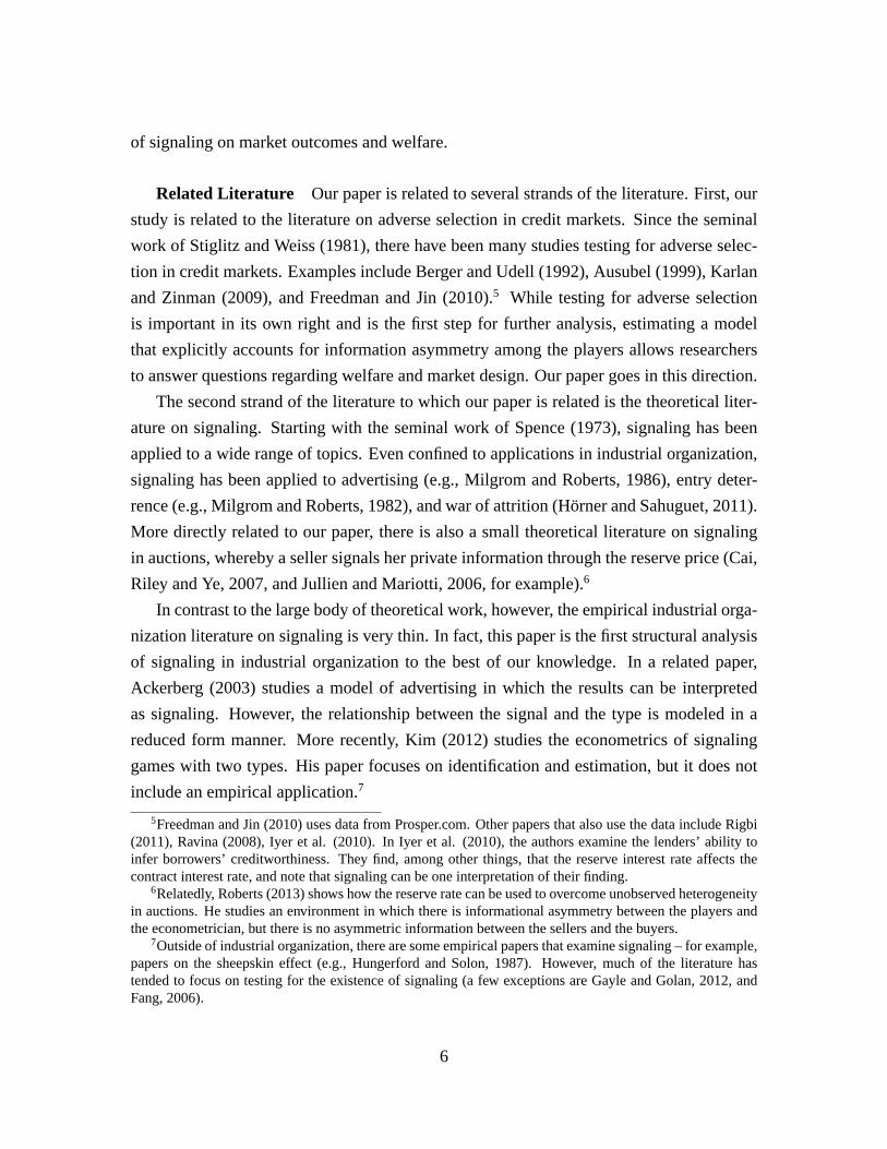
Table 1: Descriptive Statistics – Listings: This table presents summary statistics of listings posted on Pros-

per.com by credit grade. Debt/Income is the debt-to-income ratio of the borrower. Home Owner is a dummy

variable that equals 1 if the potential borrower is a homeowner and 0, otherwise. Bid Count is the number of

submitted bids by the lenders. Fund Pr. stands for the percentage of listings that are funded.

05

1015

Den

sity

0 .1 .2 .3 .4Reserve Rate

AA

05

1015

Den

sity

0 .1 .2 .3 .4Reserve Rate

A

02

46

810

Den

sity

0 .1 .2 .3 .4Reserve Rate

B

05

1015

20D

ensi

ty

0 .1 .2 .3 .4Reserve Rate

C

010

2030

40D

ensi

ty

0 .1 .2 .3 .4Reserve Rate

D

020

4060

Den

sity

0 .1 .2 .3 .4Reserve Rate

E

010

2030

4050

Den

sity

0 .1 .2 .3 .4Reserve Rate

HR

05

1015

2025

Den

sity

0 .1 .2 .3 .4Reserve Rate

All Grades

Figure 2: Distribution of Reserve Interest Rate by Credit Grade – We show the distribution of reserve interest

rate by credit grade. The reserve interest rate is capped at 36% because of the usury law.

11

0.0

5.1

.15

.2D

ensi

ty

50 100 150 200 250Amount

AA

0.0

5.1

.15

.2D

ensi

ty

50 100 150 200 250Amount

A

0.0

5.1

.15

.2D

ensi

ty

50 100 150 200 250Amount

B

0.0

5.1

.15

.2D

ensi

ty

50 100 150 200 250Amount

C

0.0

5.1

.15

.2D

ensi

ty

50 100 150 200 250Amount

D

0.0

5.1

.15

Den

sity

50 100 150 200 250Amount

E

0.0

5.1

.15

.2D

ensi

ty

50 100 150 200 250Amount

HR

0.0

5.1

.15

.2.2

5D

ensi

ty

50 100 150 200 250Amount

All Grades

Figure 3: Distribution of Bid Amount – The figure shows the distribution of bid amount for each credit

grade. Bids with amount exceeding $250 are not shown. The fraction of these bids is about 3.5%.

In Figure 3, we report the distributions of the bid amount, again by credit grade. The

fraction of lenders who bid $50 exceeds 70% across all credit grades, and the fraction of

lenders who bid $100 is more than 10% in all credit grades. Hence, more than 80% of

lenders bid either $50 or $100. We also find that a small fraction of lenders bid $200,

but rarely beyond that. These observations motivate us to formulate the potential lenders’

amount choice as a discrete–choice problem in our model section, where lenders choose

from {$50, $100, and $200} rather than from a continuous set.

Table 2 reports sample statistics of listings that were funded, which is a subset of the

set of listings. Note that the mean loan amount reported in Table 2 is smaller than the mean

requested amount shown in Table 1, which is natural given that smaller listings need to

attract a smaller number of bids in order to get funded. Also, note that the average bid

count in Table 2 is higher than in Table 1, for the obvious reason that listings need to attract

sufficient bids to get funded: Recall that there is no partial funding for listings that fail to

attract enough bids to cover the requested amount.

For each loan originated by Prosper, we have monthly data regarding the repayment

decisions of the borrower, i.e., we observe whether the borrower repaid the loan or not

every month, and whether the borrower defaulted. In the first column of Table 3, we report

sample statistics regarding the default probability by credit grade. The average default

probability is lowest for AA loans at 14.9%, while it is highest for HR loans at 43.9%.

Table 3 also reports the mean and the quantiles of the internal rate of return (IRR) of the

loans.12 The average IRR for all listings is -4.6%, and it is negative in all credit grades

12If we denote the (monthly) IRR by R, then R is the interest rate that equalizes the loan amount to the

12

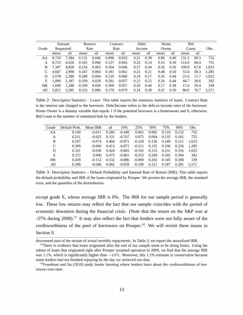
Amount Reserve Contract Debt/ Home Bid

Grade Requested Rate Rate Income Owner Count Obs.

mean sd mean sd mean sd mean sd mean sd mean sd

AA 9,710 7,384 0.131 0.046 0.096 0.033 0.21 0.39 0.80 0.40 131.5 99.3 755

A 8,723 6,626 0.165 0.060 0.127 0.045 0.23 0.14 0.55 0.50 114.0 84.4 755

B 7,347 4,858 0.216 0.063 0.164 0.046 0.27 0.34 0.56 0.50 100.9 67.6 1,023

C 4,687 2,998 0.247 0.064 0.181 0.062 0.25 0.21 0.48 0.50 53.4 38.3 1,285

D 3,578 2,380 0.280 0.064 0.210 0.066 0.24 0.17 0.26 0.44 21.6 11.7 1,022

E 1,890 1,187 0.339 0.028 0.291 0.057 0.22 0.22 0.26 0.44 44.7 30.6 392

HR 1,690 1,288 0.339 0.036 0.300 0.057 0.20 0.44 0.17 0.38 17.6 10.4 339

All 5,821 5,285 0.233 0.086 0.179 0.079 0.24 0.28 0.47 0.50 80.0 76.7 5,571

Table 2: Descriptive Statistics – Loans: This table reports the summary statistics of loans. Contract Rate

is the interest rate charged to the borrower. Debt/Income refers to the debt-to-income ratio of the borrower.

Home Owner is a dummy variable that equals 1 if the potential borrower is a homeowner and 0, otherwise.

Bid Count is the number of submitted bids by the lenders.

Grade Default Prob. Mean IRR sd 10% 25% 50% 75% 90% Obs

AA 0.149 -0.011 0.283 -0.449 0.061 0.082 0.110 0.132 755

A 0.211 -0.025 0.331 -0.767 0.072 0.094 0.135 0.181 755

B 0.297 -0.074 0.404 -0.871 -0.229 0.136 0.169 0.211 1,023

C 0.309 -0.060 0.413 -0.871 -0.211 0.135 0.196 0.256 1,285

D 0.321 -0.036 0.424 -0.865 -0.192 0.153 0.231 0.316 1,022

E 0.372 0.000 0.475 -0.861 -0.315 0.249 0.345 0.394 392

HR 0.439 -0.112 0.532 -0.886 -0.800 0.202 0.345 0.398 339

All 0.286 -0.046 0.402 -0.858 -0.100 0.121 0.187 0.281 5,571

Table 3: Descriptive Statistics – Default Probability and Internal Rate of Return (IRR): This table reports

the default probability and IRR of the loans originated by Prosper. We present the average IRR, the standard

error, and the quantiles of the distriubution.

except grade E, whose average IRR is 0%. The IRR for our sample period is generally

low. These low returns may reflect the fact that our sample coincides with the period of

economic downturn during the financial crisis. (Note that the return on the S&P was at

-37% during 2008).13 It may also reflect the fact that lenders were not fully aware of the

creditworthiness of the pool of borrowers on Prosper.14 We will revisit these issues in

Section 9.

discounted sum of the stream of actual monthly repayments. In Table 3, we report the annualized IRR.13There is evidence that loans originated after the end of our sample seem to be doing better. Using the

subset of loans that originated right after Prosper resumed operation in 2009, we find that the average IRR

was 1.1%, which is significantly higher than −4.6%. Moreover, this 1.1% estimate is conservative because

some lenders had not finished repaying by the day we retrieved our data.14Freedman and Jin (2010) study lender learning where lenders learn about the creditworthiness of bor-

rowers over time.

13

3 Evidence of Signaling Through the Reserve Rate

In this section, we provide some reduced-form evidence that the borrower’s reserve interest

rate serves as a signaling device. In particular, we first show evidence that suggests that

raising the reserve rate (1) increases the funding probability; (2) increases the contract

interest rate; and (3) increases the default probability. We next argue that, taken together,

these results suggest that the reserve rate serves as a signal.

While the baseline results that we present below are based on a relatively parsimonious

specification of the reduced form, the Online Appendix contains results from richer speci-

fications with interactions of covariates as well as specifications with additional covariates,

such as text information and more detailed credit information of the borrowers. The results

of these alternative specifications are broadly consistent with our baseline results we report

below.

Funding Probability In order to analyze the effect of the reserve rate on the funding

probability, we run a Probit model as follows:

Fundedj = 1{βssj + x′jβx+εj ≥ 0}, (1)

where Fundedj is a dummy variable for whether listing j is funded or not, sj is the reserve

rate and xj is a vector of controls that include the requested amount, the debt–to–income

ratio, dummy variables for home ownership, the credit grade, calendar month, and hour of

day the listing was created.

The first column of Table 4 reports the results of this regression. The coefficient that we

are interested in is the one on the reserve rate. As reported in the first row, the coefficient is

estimated to be 2.13 and it is statistically significant. In terms of the marginal effect, a 1%

increase in sj is associated with about 0.32% increase in the funding probability.

Contract Interest Rate Next, we run the following Tobit regression to examine the

effect of the reserve rate on the contract interest rate:

r∗j = βssj + x′jβx+εj , (2)

rj =

{r∗j if r∗j ≤ sj

missing otherwise.

14

In this expression, rj denotes the contract interest rate, r∗j is the latent contract interest

rate and xj is the same vector of controls as before. The first equation relates the latent

contract interest rate to the reserve rate and other listing characteristics. r∗j is interpreted

as the latent interest rate at which the loan is funded in the absence of any censoring. The

second equation is the censoring equation, which accounts for the fact that the contract

interest rate rj is always less than the reserve rate, sj . Note that if we were to run a simple

OLS regression of rj on sj and xj , the estimate of βs would be biased upwards because the

mechanical truncation effect would also be captured in βs.

We report the results from this regression in the second column of Table 4. As reported

in the first row, we estimated βs to be positive and significant, which seems to suggest

that a lower reserve interest rate leads to a lower contract interest rate, consistent with our

hypothesis. As we discuss next, borrowers who post high reserve rates are relatively less

creditworthy. If we take this as given, the results of regression (2) seem to suggest that

lenders charge higher interest to riskier borrowers with high reserve rates.

In addition to the Tobit model above, we also estimated a censored quantile regression

model (see, e.g., Powell, 1986) using the same specification as equation (2). The quantile

regression allows us to test whether a similar relationship between r∗j and sj that we find for

the mean holds for different quantiles. The results of the quantile regressions are qualita-

tively similar.15 The results seem to imply that F (r∗|s) first order stochastically dominates

F (r∗|s′) for s ≥ s′.

The results of the two regressions, (1) and (2), that we ran suggest that a borrower faces

a trade-off in setting the reserve price, i.e., the borrower must trade-off the increase in the

probability of acquiring a loan with the possible increase in the contract interest. Note that

it is probably safe to assume that many borrowers are actually aware of this trade-off: In a

prominently displayed tutorial, Prosper informs the borrowers that setting a higher reserve

rate increases the probability that the loan will be funded. Given the dispersion in the re-

serve rate (See Fig. 2), it is natural to think that there is unobserved borrower heterogeneity

that induces borrowers to weigh the trade-off differently. For example, if borrowers are

heterogeneous with respect to the cost of obtaining credit from outside sources, borrowers

who have low cost will tend to post low reserve rates, while those who have high cost will

post high reserve rates, giving rise to dispersion in the reserve rate.

15The results are available on request.

15

(1) (2) (3) (4)

Funded Contract Rate Default Rate of Return

Reserve rate 2.1368∗∗∗ 0.6834∗∗∗ 1.5365∗∗∗ -0.5919∗∗∗

(0.0263) (0.0145) (0.4095) (0.1313)

Contract rate 2.1531∗∗∗ 0.0540

(0.4091) (0.1372)

Amount -0.0001∗∗∗ 1.12E-06∗∗∗ 1.92E-05∗∗∗ -4.51E-06∗∗∗

(0.0000) (6.12E-06) (4.38E-06) (1.24E-06)

Debt / income -0.7971∗∗∗ 0.0731∗∗∗ 0.0275 -0.0314

(0.0015) (0.0037) (0.0588) (0.0197)

Home owner -0.1513∗∗∗ 0.0137∗∗∗ 0.0633 -0.0471∗∗∗

(0.0004) (0.0018) (0.0366) (0.0117)

Grade

AA 3.6468∗∗∗ -0.3013∗∗∗ -0.1896 0.0595

(0.0044) (0.0061) (0.1236) (0.0402)

A 3.0727∗∗∗ -0.2670∗∗∗ -0.1543 0.0475

(0.0033) (0.0055) (0.1083) (0.0366)

B 2.5681∗∗∗ -0.2347∗∗∗ -0.0888 0.0224

(0.0022) (0.0046) (0.0894) (0.0320)

C 1.8743∗∗∗ -0.1862∗∗∗ -0.0780 0.0380

(0.0014) (0.0038) (0.0777) (0.0288)

D 1.2754∗∗∗ -0.1329∗∗∗ -0.1162 0.0636∗∗

(0.0011) (0.0034) (0.0773) (0.0272)

E 0.5022∗∗∗ -0.0499∗∗∗ -0.2814∗∗∗ 0.1155∗∗∗

(0.0014) (0.0036) (0.0878) (0.0296)

Observation 35,241 35,241 85,657 5,571

R2 0.2827 0.0224

Likelihood -1,137 -4,686

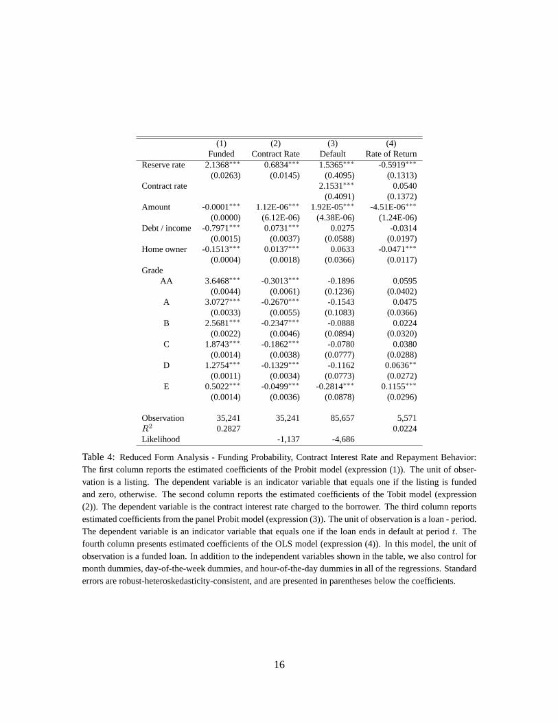
Table 4: Reduced Form Analysis - Funding Probability, Contract Interest Rate and Repayment Behavior:

The first column reports the estimated coefficients of the Probit model (expression (1)). The unit of obser-

vation is a listing. The dependent variable is an indicator variable that equals one if the listing is funded

and zero, otherwise. The second column reports the estimated coefficients of the Tobit model (expression

(2)). The dependent variable is the contract interest rate charged to the borrower. The third column reports

estimated coefficients from the panel Probit model (expression (3)). The unit of observation is a loan - period.

The dependent variable is an indicator variable that equals one if the loan ends in default at period t. The

fourth column presents estimated coefficients of the OLS model (expression (4)). In this model, the unit of

observation is a funded loan. In addition to the independent variables shown in the table, we also control for

month dummies, day-of-the-week dummies, and hour-of-the-day dummies in all of the regressions. Standard

errors are robust-heteroskedasticity-consistent, and are presented in parentheses below the coefficients.

16

Repayment Behavior We now explore the extent to which borrowers who post high

reserve rates are similar to or different from those who post low reserve rates in terms of

their ability to pay back. In order to do so, we first run a panel Probit of an indicator

variable for default on observable characteristics of the loan as well as the reserve rate:

Defaultjt = 1{βssj + βrrj + x′jβx + µt + αj + εjt ≥ 0}, (3)

where Defaultjt denotes a dummy variable that takes a value of 1 if borrower j defaults

on the loan at period t, µt is a period-t dummy, and αj is a borrower random-effect. The

coefficient βs captures the relationship between the reserve interest rate and the default

probability. Note that because we control for the contract interest rate in the regression,

the effect captured by βs is purely due to selection. Given that the reserve rate should not

directly affect the behavior of the borrower once we condition on the contract interest rate,

βs is not picking up the effect of moral hazard.

The parameter estimates obtained from this regression are shown in the third column of

Table 4. The coefficient associated with the reserve interest rate is positive and significant,

with βs = 1.54. In terms of the marginal effect, a 1% increase in sj is associated with about

1.25% increase in the default probability. This implies that borrowers who post higher

reserve interest rates tend to default more often, which is consistent with the notion that

the reserve rate is informative about the type of the borrowers, i.e., the reserve interest rate

can be used as a signal of the creditworthiness of the borrower. In the second row, we also

report our estimates of the coefficient on the contract interest rate and the coefficient on the

requested amount. We find that both coefficients are positive and statistically significant.

The positive coefficient on the contract interest rate may be capturing moral hazard – higher

interest tends to increase the probability of default. The positive coefficient on the amount

can be a result of either adverse selection or moral hazard.16

We now wish to examine how the reserve rate relates to the borrower’s repayment

behavior from the perspective of the lender. In order to do so, we analyze how the IRR is

16Borrowers who request a bigger loan may be less creditworthy, or a bigger loan may induce borrowers

to default more often because of higher interest payments. The former explanation would be consistent with

adverse selection, and the latter would be consistent with moral hazard. The borrower’s choice of the loan

size is an interesting issue, but it is hard to tease out moral hazard and adverse selection. That is one reason

why our paper focuses on the borrower’s choice of the reserve rate. Note, however, that we are not ruling

out the possibility that the loan amount can also be a signal. See sections 4.1 and 5.1 for more details. For

an analysis of the loan size and down payment in the context of subprime lending in used–car markets, see

Adams, Einav, and Levin (2009) and Einav, Jenkins, and Levin (2012).

17

related to the reserve interest rate by estimating the following model:

IRRj = βssj + βrrj + x′jβx + εj , (4)

where IRRj is the internal rate of return of loan j and xj is the same vector of observable

characteristics as before. As with our discussion of regression (3), the coefficient on sj

captures the selection effect.

The parameter estimates obtained from this regression are shown in the fourth column

of Table 4. As expected, the reserve interest rate has a negative and significant effect on the

IRR (βs = −0.59), which indicates that, on average, lenders make less money on loans that

are made to borrowers who posted high reserve interest rates.17 This is consistent with the

results of regression (3), where we examined the relationship between rj and the default

probability.

Interpretation of the Results Taken together, our regression results seem to indicate

that (1) there is a trade-off in setting the reserve rate, i.e., a trade-off between a larger

funding probability and a higher contract interest rate; (2) borrowers are heterogeneous

with respect to how they evaluate this trade-off; (3) those who post high reserve rates

tend to be relatively less creditworthy and those who post low reserve rates tend to be

relatively more creditworthy; and (4) the lenders anticipate this and charge higher interest

to riskier borrowers who post high reserve rates. These results are informative about how

signaling is sustained in equilibrium: “high cost” types, who have high cost of borrowing

from outside sources are more willing to sacrifice a favorable interest rate for a bigger

probability of being funded, while the opposite is true of the “low cost” types. Because

borrowers who post high reserve rates default relatively more often than borrowers who

post low reserve rates, “high cost” types are also less creditworthy while “low cost” types

are more creditworthy. Hence borrowers who are “low cost” and creditworthy prefer {low

interest, low probability of receiving a loan} to {high interest, high probability of receiving

a loan}, and vice versa. This prevents “bad” types from mimicking “good” types and

17This may raise the question of why lenders would choose to lend money to borrowers with a high reserve

rate (instead of lending only to borrowers with a low reserve rate). There are probably several reasons for

this. First, the contract interest rate is a random variable from the perspective of the lender and it is typically

hard to condition on the contract interest rate at the time a lender puts in her bid (Note that regression (4)

conditions on rj). Second, the lender typically pays attention to a small subset of the set of active listings

given the way they are displayed. That is, lenders may not always be aware that there are other active listings

which yield higher returns.

18

sustains separation of types through signaling.

While the results that we present in this section correspond to relatively parsimonious

specifications of the reduced form, the qualitative results are quite robust. As we discussed

before, the Online Appendix contains richer specifications where we find qualitatively sim-

ilar results. Moreover, there are papers using additional graphical and textual data that

report similar effect of the reserve rate on various outcome variables. For example, Ravina

(2008) augments the Prosper data with the perceived attractiveness of the borrowers using

the photos that borrowers post and Freedman and Jin (2010) includes variables such as so-

cial ties of the borrower, etc. Their findings are reassuring in the sense that inclusion of

these additional variables do not change much the estimated coefficients of the reserve rate

(see Table 5 of Freedman and Jin, 2010 and Table IV of Ravina, 2008).

4 Model

In this section, we develop a model of the borrowers and the lenders who participate in

Prosper, which we later take to the data. Our model has three parts. The first part of our

model concerns the reserve interest rate choice of the borrowers, the second part concerns

the lenders’ bidding behavior and the third part of our model pertains to the borrowers’

repayment behavior.

4.1 Borrowers

Borrower Repayment We first describe the repayment stage of the borrower’s de-

cision problem and work our way backwards. We model the repayment behavior of the

borrower as a sequential decision of 36 (= T ) months, which is the length of the loans that

Prosper originates. We write the terminal decision of the borrower at period T as follows:{full repayment: if uT (r) + εT ≥ D(ϕ)

default: otherwise,(5)

where uT (r) + εT denotes the period utility of the borrower if he repays the loan in full

and r denotes the interest rate on the loan. We let ϕ denote the (unobservable) type of the

borrower, which shifts the cost of defaulting, and we letD(ϕ) denote the cost of defaulting.

We can assume without loss of generality that D(ϕ) is monotonically decreasing in ϕ, i.e.,

the disutility of defaulting is larger for borrowers with higher ϕ. Hence borrowers with

19

high ϕ are “good” types who value avoiding default and maintaining a good credit history.

We assume ϕ to be independent of εT , conditional on observables. The conditional inde-

pendence of εT and ϕ may appear to be a very strong assumption, but mean independence

is actually without loss of generality. To see this, if E[εT |ϕ] 6= 0, we can subtract E[εT |ϕ]

from both sides of equation (5) and by appropriately redefining D(·) and εT , we have an

observationally equivalent model with E[εT |ϕ] = 0. This is possible because we allow

D(·) (or equivalently, the distribution of ϕ) to be nonparametric. While mean indepen-

dence is not the same as independence, we think that this alleviates some of the concerns

regarding our assumption. We come back to this point at the end of this section.

Now let VT denote the expected utility of the borrower at the beginning of the final

period T , defined as VT (r, ϕ) = E[max{uT (r) + εT , D(ϕ)}]. Then, the decision of the

borrower at period t < T is as follows:{repayment: if ut(r) + εt + βVt+1(r, ϕ) ≥ D(ϕ)

default: otherwise,

where ut(r) + εt is the period t utility of repaying the loan, β is the discount factor, and

Vt+1(r, ϕ) is the continuation utility, which can be defined recursively. We allow ut to

depend on t in order to capture any deterministic time dependence while we assume {εt}to be i.i.d across t and mean zero.

We have presented the model up to now without making explicit the dependence of the

primitives of the model on observable borrower/listing characteristics such the credit grade.

This is purely for expositional purposes. In our identification and estimation, we let ut, Fεt ,

and Fϕ depend on observable characteristics. In particular, we allow Fεt and Fϕ to depend

on observable characteristics in an arbitrary manner in our identification.

Borrower Reserve Rate Choice Now we describe our model of the borrower’s re-

serve interest choice. When the borrower determines the reserve interest rate, s, he has to

trade off its effect on the probability that the loan is funded, and its effect on the contract

interest rate, r. The borrower’s problem is then to choose s, subject to the usury law limit

of 36%, as follows:

maxs≤0.36

V0(s, ϕ) = maxs≤0.36

[Pr(s)

∫V1(r, ϕ)f(r|s)dr + (1− Pr(s))λ(ϕ)

], (6)

20

where Pr(s) is the probability that the loan is funded, f(r|s) is the conditional distribution

of the contract interest rate given s, and λ(ϕ) is the borrower’s utility from the outside

option, i.e., the borrower’s utility in the event of not obtaining a loan from Prosper. We

suppress the dependence of Pr(s) and f(r|s) on the characteristics of the borrower. Al-

though Pr(s) and f(r|s) are equilibrium objects, they are taken as exogenous and known

by the borrower. Note that another important choice variable for the borrower is the loan

amount. We treat the loan amount as part of the set of conditioning variables. We come

back to this point at the end of this section.

The first term in the bracket in equation (6) captures the borrower’s expected utility

in the event of obtaining a loan through Prosper: V1(r, ϕ), which is the value function of

the borrower at period t = 1, is integrated against the distribution of the contract interest

rate f(r|s). The second term captures the utility of the borrower in the event the loan is

not funded: (1 − Pr(s)) is the probability that this event occurs, which is multiplied by

the utility of the outside option, λ(ϕ). We assume that λ(ϕ) is increasing in ϕ, where ϕ

is the private type of the borrower we defined earlier. This assumption simply reflects the

idea that “good” types (high ϕ), who value their credit history, for example, have an easier

time obtaining a loan from outside sources, such as relatives, friends, and local banks, etc.,

and hence have a high λ(ϕ). On the other hand, “bad” types, with low cost of default,

e.g., borrowers who have a damaged credit history or are expecting to default in the future

anyway, are likely to have only limited alternative sources of funding, and hence have a

low λ(ϕ).

The first–order condition associated with problem (6) is as follows,

∂

∂sPr(s)

(∫V1(r, ϕ)f(r|s)dr − λ(ϕ)

)+ Pr(s)

∫V1(r, ϕ)

∂

∂sf(r|s)dr = 0, (7)

for an interior solution. Equation (7) captures the trade-off that the borrower faces in deter-

mining the reserve interest. The first term is the incremental utility gain that results from

an increase in the funding probability, and the second term is the incremental utility loss

resulting from an increase in the contract interest rate.

Recall from the previous section that we found strong evidence that Pr(s) is increasing

in s and that F (r|s) first order stochastically dominates F (r|s′) for s ≥ s′, where F (r|s) is

the conditional CDF of r. We note that under these conditions, the single crossing property

(SCP) is satisfied for s < 0.36. From the perspective of the borrower, SCP is necessary and

21

sufficient to induce separation. Hence there is no pooling among types below the usury law

maximum and pooling occurs only at the maximum. We state this as a proposition below.

Proposition 1 If ∂∂s

Pr(s) > 0 and F (r|s) FOSD F (r|s′) for s′ > s, then we have SCP,

i.e.,∂2

∂s∂ϕV0(s, ϕ) < 0.

To see the intuition for why SCP holds, consider the marginal utility from increasing

s, ∂∂sV0(s, ϕ), for a given type ϕ. As we explained above, ∂

∂sV0(s, ϕ) has two components.

One is the incremental utility gain from an increase in the funding probability, and the

other is the incremental utility loss resulting from an increase in the contract interest rate.

The first component is decreasing in ϕ, because borrowers with high ϕ already have a high

outside option – these borrowers do not appreciate the increase in the funding probability

as much as low ϕ types. The second component is also decreasing in ϕ, because borrowers

with high ϕ are likely to bear the full cost of an increase in r, while borrowers with low ϕ

will not – the low ϕ types will default with high probability anyway.18 A formal proof of

this proposition as well as all other proofs are contained in the Appendix.

Before turning to the lenders’ model, we briefly discuss the optimal reserve rate choice

of the borrowers when the usury law limit is binding. Recall from our discussion of Figure 2

that there is a non-negligible mass at exactly 36% for credit grades B and below, implying

that the usury law maximum is a binding constraint for many borrowers in these credit

grades. For credit grades B and C, the pattern in the data seem broadly consistent with

partial pooling, i.e., separation of types below 36%, and pooling at 36%. For there to

be partial pooling, we need an extra condition to hold (in addition to the requirements in

Proposition 1) that prevents the pooled types from deviating. We describe these conditions

in the Online Appendix. For these two credit grades, we will use them in our estimation

accounting for the fact that there is separation of types below 36%, and some pooling at

36%. For credit grades D and below, an even larger fraction of the borrowers submit a

reserve interest rate at the usury law maximum, leaving little variation in the reservation

interest rate. This means that data from these categories are not very informative about the

signaling value of the reserve rate. Hence in our estimation, we only focus on credit grades

AA, A, B, and C.

18Conditional on default, the borrower does not have to bear the full cost of a high interest rate.

22

4.2 Lenders

In this subsection, we describe the model of the lenders. Let N be the (random) num-

ber of potential lenders. We let FN denote its cumulative distribution function with sup-

port {0, 1, · · · , N̄}, where N is the maximum number of potential lenders. The potential

lenders are heterogeneous with regard to their attitude toward risk and with regard to their

opportunity cost of lending.

Each potential lender must decide whether to submit a bid or not and what to bid if

she does, where a bid is an interest-amount pair. At the time of bidding, a potential lender

observes the active interest rate in addition to various characteristics of the listing, such as

the reserve rate. In principle, the lender is free to bid any amount between $50 and the full

amount requested by the borrower, but as we showed in Section 2, the vast majority of the

bid amounts are either $50, $100, or $200. We therefore proceed with the assumption that

lenders face a discrete set of amount {$50, $100, $200} to choose from.

Lender’s Problem with No Amount Choice We first describe the case when the

lender can only bid $50, so that the lender’s decision is whether to bid or not and what

interest rate to bid. Before the lender can decide what to bid, the lender must first form

beliefs over the return she will make if she funds a part of the loan. We assume that lenders

have rational expectations, i.e., the lenders’ beliefs coincide with the realized distribution

of returns. We discuss this assumption at the end of this section.

Following the standard specification used in the asset pricing literature, we assume that

the lender’s utility from owning an asset depends on the mean and variance of the return on

the asset. Thus, we specify the utility of lender j who lends to listing Z at contract interest

rate r, as follows:

U = ULj (Z(r))− ε0j

where ULj (Z(r)) = µ(Z(r))− Ajσ2(Z(r))− c.

Note that Z(r) is the random return from investing in Z at rate r, and µ(Z(r)) and σ2(Z(r))

are its expected return and variance. Aj is a lender specific random variable known only to

lender j that determines her attitude toward risk and c and ε0j are deterministic and random

opportunity costs of lending to listing Z. c and ε0j can be interpreted as the opportunity

cost of taking money away from an existing asset in the portfolio or as a reduced form way

23

Figure 4: Graphical Representation of the Lender’s Problem: Case of No Amount Choice – The figure

illustrates how the lender should bid when there is no amount choice. In the left panel, the horizontal axis

is σ2 and the vertical axis is µ. For each listing and for each realization of the contract interest rate, we

can assign a corresonding point on this µ − σ2 plane. Curve C corresponds to the mean and variance of a

listing for different realizations of r. The dashed line is the lender’s indifference curve. The right panel plots

ULj (Z(r)) against r.

of capturing the opportunity cost of investing in other listings on Prosper.19 The outside

option is normalized to zero.

In order to study the lender’s problem, it is useful to illustrate it graphically. Figure 4 is

a graphical representation of the lender’s problem. In the left panel of this figure, we take

σ2 to be the horizontal axis and µ to be the vertical axis. Now, consider a listing Z. For

each realization of the contract interest rate, consider the mean return, µ(Z(r)), and the

variance of the return, σ2(Z(r)). Note that we can plot the points (µ(Z(r)), σ2(Z(r))) on

this µ− σ2 plane.

Curve C in the left panel of Figure 4 illustrates the possible mean and variance for a

given listing. The end point of the curve corresponds to the return and variance associated

with the case when the listing is funded at the reserve rate, so that r = s. As the contract

rate is bid down from s, the corresponding point on the µ − σ2 plane changes, and this is

shown as a movement along Curve C in the direction of the arrows. Note that we have also

drawn a dashed line in the left panel of Figure 4. This is the lender’s indifference curve,

i.e., the set of points that makes the lender indifferent between lending and not lending.

As the lender’s utility function is linear with respect to µ and σ2, the indifference curve is

a straight line, i.e., µ − Ajσ2 − c − ε0j = 0. Any point above this line gives the lender

a strictly higher utility than the outside option, and vice versa. As drawn in the Figure,

19In our identification and estimation, we assume that ε0j is i.i.d. across j conditional on a set of time

dummies. In other words, we require independence of ε0j , but only net of possible aggregate shocks.

24

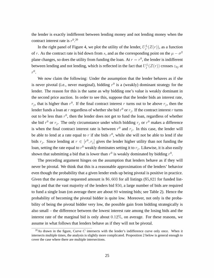
the lender is exactly indifferent between lending money and not lending money when the

contract interest rate is r0.20

In the right panel of Figure 4, we plot the utility of the lender, ULj (Z(r)), as a function

of r. As the contract rate is bid down from s, and as the corresponding point on the µ− σ2

plane changes, so does the utility from funding the loan. At r = r0, the lender is indifferent

between lending and not lending, which is reflected in the fact that ULj (Z(r)) crosses ε0j at

r0.

We now claim the following: Under the assumption that the lender behaves as if she

is never pivotal (i.e., never marginal), bidding r0 is a (weakly) dominant strategy for the

lender. The reason for this is the same as why bidding one’s value is weakly dominant in

the second price auction. In order to see this, suppose that the lender bids an interest rate,

rj , that is higher than r0. If the final contract interest r turns out to be above rj , then the

lender funds a loan at r regardless of whether she bid r0 or rj . If the contract interest r turns

out to be less than r0, then the lender does not get to fund the loan, regardless of whether

she bid r0 or rj . The only circumstance under which bidding rj or r0 makes a difference

is when the final contract interest rate is between r0 and rj . In this case, the lender will

be able to lend at a rate equal to r if she bids r0, while she will not be able to lend if she

bids rj . Since lending at r ∈ [r0, rj] gives the lender higher utility than not funding the

loan, setting the rate equal to r0 weakly dominates setting it to rj . Likewise, it is also easily

shown that submitting a bid that is lower than r0 is weakly dominated by bidding r0.

The preceding argument hinges on the assumption that lenders behave as if they will

never be pivotal. We think that this is a reasonable approximation of the lenders’ behavior

even though the probability that a given lender ends up being pivotal is positive in practice.

Given that the average requested amount is $6, 603 for all listings ($5,821 for funded list-

ings) and that the vast majority of the lenders bid $50, a large number of bids are required

to fund a single loan (on average there are about 80 winning bids; see Table 2). Hence the

probability of becoming the pivotal bidder is quite low. Moreover, not only is the proba-

bility of being the pivotal bidder very low, the possible gain from bidding strategically is

also small – the difference between the lowest interest rate among the losing bids and the

interest rate of the marginal bid is only about 0.12%, on average. For these reasons, we

assume in what follows that lenders behave as if they will not be pivotal.

20As drawn in the figure, Curve C intersects with the lender’s indifference curve only once. When it

intersects multiple times, the analysis is slightly more complicated. Proposition 2 below is general enough to

cover the case where there are multiple intersections.

25

Lender’s Problem with Amount Choice Thus far, our discussion has considered the

case with no amount choice for the lenders. Now consider the case with amount choice,

where the borrower chooses q from the setM = {50, 100, 200} or chooses not to bid. Note

that if the lender bids amount q to listing Z at contract interest rate r, then E[qZ(r)] =

qµ(Z(r)) and V ar(qZ(r)) = q2σ2(Z(r)). Hence, lender j’s utility can be expressed as

follows,

U = ULj (qZ(r))− ε0j = qµ(Z(r))− Aj(qσ(Z(r)))2 − cq − ε0j , (8)

where the cost of lending now depends on q as cq.

When the lender faces an amount choice, she needs to keep track of the utility asso-

ciated with all possible actions. This is depicted in Figure 5. The three curves in Figure

5 correspond to ULj (50Z(·)), UL

j (100Z(·)), and ULj (200Z(·)). Just as before, there is a

(weakly) dominant strategy for the lender under the assumption that the bidder is not piv-

otal. For the case shown in Figure 5, a (weakly) dominant strategy can be described by the

following bid strategy:

bid amount $200 and interest r′ if active interest rate ∈ [r′, s]

bid amount $100 and interest r′′ if active interest rate ∈ [r′′, r′)

bid amount $50 and interest r′′′

if active interest rate ∈ [r′′′, r′′)

do not bid if active interest rate ∈ [0, r′′′),

where the active interest rate is understood to be equal to s if the listing has not attracted

enough bids to reach the requested amount. We now state the previous analysis in the form

of a proposition.

Proposition 2 Define a partition I0 = [0, r1], I1 = [r1, r2],· · · IM = [rM , s], and a corre-

sponding quantity for each interval, q(0), q(1),· · · , q(M), where q(k) ∈ {$0}∪M , so that

ULj (q(k)Z)− ε0j ≥ UL

j (q′Z)− ε0j for all q′ and r ∈ Ik.21 Under the assumption that the

lender behaves as if she is never pivotal, it is a dominant strategy to bid q(k) and interest

rate rk when the active interest rate is in Ik.

We conclude the lender’s model by briefly discussing the relationship between the

model and identification. Using the ex-post borrower repayment data, we can identify the

21To be more precise, when q(k) 6= 0, ULj (q(k)Z)−ε0j ≥ max{0,maxq∈M ULj (q(k)Z)−ε0j} and when

q(k) = 0, 0 ≥ maxq∈M ULj (q(k)Z)− ε0j .

26

Figure 5: Graphical Representation of the Lender’s Problem: Case of Amount Choice – The figure illustrates

how the lender should bid when there is amount choice. Each curve ULj (qZ(r)) illustrates the relationship

between r and the lender’s utility net of ε0j when the lender bids q. I1 corresponds to the region of the active

interest rate for which bidding $200 is optimal. I2, I3, and I4 correspond to the regions of the active interest

rate for which bidding $100, $50, and $0 is optimal, respectively.

µ(Z(r)) and σ(Z(r)) for each r. In particular, we can identify µ(Z(s)) and σ(Z(s)), where

s is the reserve interest rate, i.e., we can identify the “starting end point” of Curve C for

any listing. This means that for each distribution of A and N (the risk aversion parameter

of the lender and the number of potential lenders) the lenders’ bidding strategy described

above will induce a probability distribution over (i) whether a listing is funded and (ii) the

number of lenders who bid $0, $50, $100, and $200 for listings that are not funded. In the

next section, we show that this mapping from the primitives to the probability distribution

over (i) and (ii) is actually a one-to-one mapping. Correspondingly, our estimation is based

on matching the predicted distribution with the sample distribution.

4.3 Equilibrium

We now discuss equilibrium existence and uniqueness. There always exists an equilibrium

of the model we described, but there may not exist a separating equilibrium.22 General

sufficient conditions for the existence of a separating equilibrium are provided in Mailath

(1987). While it is relatively straightforward to check whether the model satisfies the suffi-

cient conditions in Mailath (1987) for a given parameter value, it is not easy to analytically

characterize the set of parameters that satisfy these conditions. In what follows, we pro-

22There always exists a pooling equilibrium. As long as the lenders’ beliefs off the equilibrium path are

sufficiently pessimistic, all borrowers will find it optimal to post the same reserve rate.

27

ceed by estimating the model assuming that the agents are playing a separating equilibrium.

Once we have estimated our parameters, we then check whether the sufficient conditions

for separation are satisfied at the estimated values.23 At the estimated parameter values, the

conditions seem to generally hold.

As for uniqueness, signaling models generally admit multiple equilibria because there

are always pooling equilibria in which no information is transmitted. It turns out, however,

that under a mild assumption on the beliefs over borrower types off the equilibrium path,

there is a unique separating equilibrium (see Mailath, 1987). Given our regression results

from section 3, assuming that the agents are playing a separating equilibrium is not unrea-

sonable. Hence, as long as the assumptions on the off-path beliefs are satisfied, we do not

need to worry about multiple equilibria.

4.4 Model Discussion

In this section, we discuss some of our modeling choices and assumptions.

Independence of εt and ϕ An important assumption we made in our borrower’s re-

payment model is the independence of εt and ϕ. While independence is a restrictive as-

sumption, we note that mean independence of εt, i.e., E[εt|ϕ] = 0, is without loss of

generality. This is because we can always redefine εt and ϕ – redefine εt as (εt − E[εt|ϕ])

and D(·) as (D(·)− E[εt|·]) – so that E[εt|ϕ] = 0. Given that we allow D(·) (or equiva-

lently, the distribution of ϕ) to be nonparametric in our identification and estimation, this is

without loss of generality. Of course, mean independence is not the same as independence

of εt and ϕ, but it does give some credibility to the independence assumption. Relatedly,

we only require independence εt and ϕ conditional on listing characteristics. Conditional

independence is a weaker assumption because it allows for εt and ϕ to be correlated un-

conditionally.

23The condition identified in Mailath (1987) is a monotonicity requirement on the borrower’s utility func-

tion,∂

dsV0(s, ϕ, ϕ̃;X)

/∂

dϕ̃V0(s, ϕ, ϕ̃;X) is increasing in ϕ, ∀ϕ,∀X ,

where V0(s, ϕ, ϕ̃;X) is the borrower’s expected utility from posting a reserve interest rate s, when the bor-

rower is of type ϕ, and the lenders perceive him to be of type ϕ̃. X is a vector of conditioning variables such

as borrower and listing characteristics. The reason why we don’t include this condition in our estimation

routine is because we need to verify whether the monotonicity requirement is satisfied for all X . It would be

computationally impossible to include this condition in the estimation routine.

28

Serial Correlation in εt Another assumption we made in our borrower’s repayment

model is the independence of {εt} across t. Note that what we observe in the data are

a sequence of binary decisions (repay or default) for each borrower, in which default is

an absorbing state: If a borrower defaults, we do not observe any repayment decisions

from that point on. Unlike in a situation where there are distinct decisions for each of

the T periods (i.e., no absorbing state), our particular data structure precludes us from

identifying possible serial correlation in {εt}.24 Only the marginals of {εt} are relevant

for data generation. While this may appear to be a limitation, this means that under the

assumption that {εt} is structural, our counterfactual policy is robust to serial correlation

among {εt}.

Interpretation of ϕ Recall that the unobservable type of the borrower (ϕ) is inter-

preted as default cost in our model. However, we can write an alternative, observationally

equivalent model where ϕ has the interpretation of unobserved income/assets of the bor-

rower. We show this in the Online Appendix. While there are several ways to model bor-

rower heterogeneity – default cost, income, or some combination of the two – the implied

default pattern may be very similar. For our purposes, the exact nature of heterogeneity

among the borrowers is not very important because it is structural to our counterfactual

policy. This is not to say, however, that the distinction may be very important in other

contexts.

Signaling through the Loan Amount In addition to the reserve interest rate, an im-

portant variable that the borrower needs to optimize over is the requested amount. We do

not explicitly model the amount choice of the borrower and instead focus only on the re-

serve rate choice. First of all, the reserve rate choice offers a cleaner setting to analyze

the effect of signaling. Given that the reserve rate should not affect the lender’s repayment

behavior conditional on the contract interest rate, the correlation between the reserve rate

and the default probability is informative about the pure informational value of the reserve

24Consider an extreme case when {εt} takes on only two values, {+∞,−∞}. The following two cases

are observationally equivalent: (1) {εt} are perfectly correlated, so ε1 = · · · = εT , and Pr(ε1 = +∞) = p(2) {εt} are independently distributed, with Pr(ε1 = +∞) = p, and εt = +∞ with probability 1 for all

t ≥ 2. For case (1), either ε1 = · · · = εT = +∞ or ε1 = · · · = εT = −∞ with probability p and 1 − p.

For case (2), ε1 = +∞ or ε1 = −∞ with probability p and 1 − p, but εt = +∞ with probability 1 for

all t ≥ 2. Note that The two cases are different, but we cannot identify between (1) and (2): In both cases,

the borrower would default with probability p in the first period, and conditional on not defaulting in the

first period, the borrower never defaults later. Our counterfactual results would be the same under either data

generating process.

29

rate as a signal. On the other hand, the requested amount can affect the default probability

both through informational channels as well as through moral hazard.

Moreover, note that focusing only on the reserve rate choice and abstracting away from

the amount choice does not bias our results in any way for the following two reasons. First,

even when the borrower optimizes over the requested amount, the borrower still chooses

the reserve rate in accordance with equation (6). That is, conditional on the amount the bor-

rower requests, the reserve interest rate still solves equation (6). Second, we are allowing

ϕ to be (arbitrarily) correlated with the requested amount, allowing for the possibility that

the requested amount can be informative about ϕ. All of our model and estimation can thus

be described as conditional on the requested amount and the results we obtain are robust to

this abstraction.

Rational Expectations The lenders in our model form beliefs over the distribution of

the return on the loans when they make their bidding decisions. For our baseline results, we

assume rational expectations, i.e., the lenders’ beliefs coincide with the realized distribution

of returns – which can be backed out directly from the data. The rational expectations

assumption is convenient, but there are several reasons why this may not hold in our sample.

For example, our data covers the period soon after the launch of Propser and lenders may

have had optimistic beliefs at the beginning. Our data also coincides with the period of the

financial crisis which may have been largely unexpected by the lenders. In order to check

the robustness of our results to the assumption of rational expectations, we estimate our

model under alternative beliefs. The robustness results are presented in Section 9.

Cost of Revising the Bid The optimal strategy described in Proposition 2 requires

the lenders to submit new bids as the active interest rate changes. In the situation depicted

in Figure 5, for example, the lender would submit new bids as the active interest rate drops

below r′, r′′, and r′′′. This implicitly takes as given that lenders have low cost of revising

their bid.25 While this may be a strong assumption, it allows us to abstract from the dynam-

ics of bidding and increases the tractability of the model. Also, in order to make sure that

our estimates are not too sensitive to this assumption, we do not use the full implications

of the dominant strategy (For example, we do not use the exact distribution of the realized

25Some bidding strategies can be replicated with a one-time proxy bid. For example, one can submit four

$50 bids, two bids with interest rate r′, and two others with r′ and r′′, respectively. This bidding strategy is

equivalent to the dominant strategy we described for Figure 5.

30

contract interest rate). Our estimation only uses moments that are not too sensitive to this

assumption as we describe below.

5 Identification

5.1 Identification of the Borrower’s Primitives

The primitives of the borrower that we would like to identify are the period utility function,

ut(·), the distribution of borrower types, Fϕ|X , the cost of default, D(·), the utility from

the outside option, λ(·), and the distribution of εt, Fε|X . We specify ut to depend on the

repayment amount and a time trend as ut(r) = −(r × xamt) + dt, where xamt is the loan

size and dt is a period specific constant term.

We begin with a few remarks. First, note that we allow the distribution of ϕ, Fϕ|X , as

well as the distribution of εt, Fε|X , to depend on borrower/listing characteristics, X . In

particular, the distribution of ϕ can depend on the amount requested. To the extent that

there is some signaling value in the requested amount, the conditional distribution of ϕ will

depend on the amount requested. We are allowing for this possibility. Second, note that

we can normalize either D(·) or Fϕ|X (for some X = X∗) without loss of generality. For

identification (and estimation) we normalize D(ϕ) = −ϕ.26 It is also easy to see that we

can normalize one of the constants in ut without loss of generality: Hence we set dT = 0.27

The intuition for our identification is quite simple. Recall that we model the borrowers’

repayment decision as a sequence of binary decisions. Hence, if we knew the value of ϕ for

each borrower, our model is a simple binary threshold crossing model and identification of

the primitives easily follow from existing results (See, e.g., Mazkin (1992)).28 The question

then becomes how we identify ϕ. The identification of ϕ relies on the observation that

there is a one-to-one (monotonic) mapping of s to ϕ conditional on X (for the case of

no pooling). Recall from Proposition 1 that the objective function of the borrower when

choosing s (see equation (6)) satisfies the single crossing property. This guarantees that

types with higher ϕ choose lower s conditional on X . In particular, if we take loans for

26This is because a specification with D̃(ϕ) = −ϕ, F̃ϕ|X = Fϕ|X ◦ D−1, and λ̃ = λ ◦ D−1 is going

to be observationally equivalent to one with D, Fϕ|X , and λ. The important component of the model is the

distribution of D(ϕ), rather than the distribution of ϕ or the shape of D(·) per se.27If we set d̃t = dt + κ (∀t) ε̃t = εt − κ (∀t), it will be observationally equivalent to dt, Fε|X .28To be precise, the binary threshold crossing model identifies Fεt|X∗ for some X∗. In order to identify

Fεt|X∗ for X 6= X∗, we also use the first-order condition (7). Once Fϕ|X and Fε|X are identified, λ(·) is

identified from equation (7).

31

which the reserve rate is equal to the α quantile of Fs|X , the borrowers all have ϕ equal to

the 1− α quantile of Fϕ|X . Then the default rate among borrowers with reserve rate equal

to F−1s|X(α) identifies Fϕ|X(α) (and hence the value of ϕ for each borrower). The following

proposition states our results formally:

Proposition 3 Fϕ|X , Fε|X and λ(·) are nonparametrically identified up to location normal-

izations. {dt} are also identified.

Nonparametric identification of Fϕ|X , Fε|X and λ(·) holds even when there is partial

pooling at 36%. The proof of this Proposition when there is no pooling appears in the

Appendix. The Online Appendix contains the proof of the proposition when there is partial

pooling.

5.2 Identification of the Lender’s Primitives

The primitives of the lender’s model that we need to identify are the distribution of the

coefficient of risk, FA, the distribution of the outside option, Fε0 , the cost of lending, cq,

and the distribution of the number of potential bidders, FN , which is assumed to have finite

support {1, .., N}. Our proof of identification proceeds by first showing identification of

FA, Fε0 , and cq under the assumption that Pq(µ, σ), which we will define below, is identified

for all values of (µ, σ) and q ∈ M ∪ {$0} ≡ {$0, $50, $100, $200}. We will then show

that Pq(µ, σ) and FN are identified. For each q ∈M ∪ {$0}, define Pq(µ, σ) as follows:

Pq(µ, σ) =

Pr

(qµ− A(qσ)2 − cq − ε0 ≥ max

{0,max

q′∈M{q′µ− A(q′σ)2 − cq′ − ε0}

})for q ∈M

Pr(0 ≥ maxq′∈M{q′µ− A(q′σ)2 − cq′ − ε0}) for q = 0

.

Pq(µ, σ) is the probability that funding q dollars gives higher utility than funding q′ (q′ 6= q)

dollars given a listing with mean and variance of return equal to µ and σ2. Note that

Pq(µ, σ) corresponds to the probability that (A, ε0) lie in the region defined by the inequal-

ities in the expression above. By varying µ and σ, this region changes. Proposition 4

claims that with enough variation in µ and σ, we can recover the probability that (A, ε0)

is contained in an arbitrary set, i.e., identify FA and Fε0 .29 In other words, (FA, Fε0 , cq) is

identified if Pq(µ, σ) are identified.

29Our identification strategy is similar to the one taken in Cohen and Einav (2007).

32

Proposition 4 There is a one-to-one mapping from (FA, Fε0 , cq) to (Pq(µ, σ), P0(µ, σ)).

The next proposition claims that Pq(µ, σ) and FN are both identified.

Proposition 5 Pq(µ, σ) is identified for all q and (µ, σ) on the support of (µ, σ). FN is

also identified.

The proof of Propositions 4 and 5 are contained in the Online Appendix. Here, we

briefly discuss the intuition for why FN and Pq(µ, σ) are identified. Consider a listing

which has yet to be fully funded. Let xamt denote the requested loan amount and (µ,

σ2) denote the mean return and variance of this listing if funded at the reserve interest,

s. Under the strategy described in section 4.2, a lender bids an amount equal to qj if and

only if lender j’s risk aversion parameter and the outside option, (Aj ,ε0j), are such that

ULj (qZ(s)) − ε0j ≥ max{maxq′∈M UL

j (q′Z(s)) − ε0j, 0}. The probability of this event is

Pq(µ, σ). Given that a listing is funded if and only if there is a sufficient number of potential

bidders who are willing to fund it, we can express the probability that a listing is funded,

as a function of FN , and {Pq(µ, σ)}. Since the probability that a listing is funded can be

identified for all xamt, µ, and σ2, if we assume that FN is invariant to xamt and (µ, σ),

sufficient variation in xamt and (µ, σ) identifies both FN and Pq(µ, σ).30

Our identification relies on the fact that when a lender with (Aj , ε0j) visits a listing that

is still not fully funded, the lender submits a bid with amount q if and only if ULj (qZ(s))−

ε0j ≥ max{maxq′∈M ULj (q′Z(s)) − ε0j, 0}, where Z(·) is evaluated at the return from

funding the listing at s. Note that this lender behavior is consistent with the dominant

strategy we described in section 4.2.

6 Estimation

We estimate our model in three steps. First, we estimate the conditional distribution of the

contract interest rate given the reserve rate, f(r|s, x), and the funding probability, Pr(s, x).

We estimate these two functions nonparametrically as f(r|s, x) and Pr(s, x) are both equi-

librium objects. The second step involves estimating the primitives of the model of the

borrower, and in the last step, we estimate the model of the lender. While our discussion

of identification in the previous section focused on nonparametric identification, we place

30Assuming that there is rich variation in xamt is a bit problematic because the borrowers cannot request

more than $25, 000 i.e., xamt ≤ 25000.

33

parametric functional forms for some of the model primitives in our estimation, as we will

describe below.

6.1 Estimation of f(r|s, x) and Pr(s, x)

Our estimation proceeds first by estimating f(r|s, x) and Pr(s, x), where x is a vector

of observable listing characteristics such as the credit grade, requested amount, debt-to-

income ratio, and home ownership. We use a (second-order) Hermite series approximation

to estimate f(r|s, x), following Gallant and Nychka (1987). Our estimation of Pr(s, x) is

based on a Probit model with flexible functional forms. The details regarding the estimation

are contained in the Online Appendix.

6.2 Estimation of the Borrower Model

We parameterize the borrower’s period t utility function and outside option with parameters

θB and denote them by ut(r, xamt; θB) and λ(ϕ; θB). The default cost D(ϕ) is normalized

as D(ϕ) = −ϕ (see Section 5.1).

In order to estimate θB, we maximize the likelihood with respect to the repayment

behavior of each borrower. Note that for any θB, our borrower’s repayment model gener-

ates a probability distribution over sequences of repayment and default decisions for each

borrower type ϕ. Given that we do not observe ϕ, we cannot use the probability distrib-

ution directly to form a likelihood. Recall, however, that there is a monotone relationship

between ϕ and s (conditional on x), where this relationship is implicitly defined by the

borrower’s first-order condition (equation (7)). This means that we can back out the type

of the borrower from his choice of s by using the first order condition. Once we can assign

a ϕ for each borrower, we can then compute the likelihood.

The actual computation of the likelihood proceeds as follows: First, recall that the

borrower’s choice of the reserve rate satisfies the first-order condition;

∂ Pr(s, x)

∂s

(∫V1(r, ϕ, x; θB)f(r|s, x)dr − λ(ϕ; θB)

)+Pr(s, x)

∫V1(r, ϕ, x; θB)

∂f(r|s, x)

∂sdr = 0.

(9)

Given that we observe the reserve rate chosen by each borrower, this equation can be seen

as an equation in ϕ. In other words, the first-order condition reveals, for each choice of

s, the type of borrower ϕ who found it optimal to choose s. Since we have estimated

Pr(s, x) and f(r|s, x) in the first step, we can replace these objects with our nonparametric

34

estimates P̂r(s, x) and f̂(r|s, x). We can also compute V1(r, ϕ, x; θB) for each value of

{r, ϕ, x} given θB by recursively solving the borrower’s dynamic problem. This allows us

to back out the borrower’s type, ϕ̂ ≡ ϕ̂(s, x; θB), for each borrower. Note that Proposition

1 shows that the right-hand side of equation (9) is monotonic in ϕ, guaranteeing a unique

solution given s and x (for unpooled types).31

The second step of our procedure is to compute the likelihood for a given sequence of

repayment decisions for each borrower i, using ϕ̂i = ϕ̂(si, xi; θB). Borrower i’s default

probability at period t is

Pr(default at t; θB) =

∫1 {−ϕ̂i ≥ ut(ri, xi,amt; θB) + dt + εit + βVt+1(ri, ϕ̂i)} dFε|x,

(10)

and the probability of paying back at period t is 1 − Pr(default at t; θB). Let ιit be an

indicator variable that is equal to 1 if borrower i defaults at period t, and 0 otherwise.

Finally, the likelihood is written as

L(θB) =

NL∏i=1

[Ti∏t=1

Pr(default at t; θB)ιit × Pr(repay at t; θB)(1−ιit)

], (11)

where NL is the number of loans, {ιit}, is the sequence of repayment decisions, and Ti ≡max{1 +

∑Tτ=1 ιiτ , 36}, i.e., the number of periods until default or 36 periods, whichever

is smaller. We obtain our parameter estimates by maximizing the likelihood function.32

31In practice, there are a few borrowers (less than 10% of the sample) for whom we could not solve for

ϕ̂(s, x; θB) even when s < 36%. This would happen if the single-crossing condition is not satisfied for a

given (s,x), i.e., f(r|x, s) does not satisfy FOSD or Pr(s, x) is not increasing at (s,x).

In principle, Mailath (1987) gives conditions under which a separating equilibrium exists (in particular,

these conditions imply that the single crossing property for the borrowers is satisfied for equation (9)). We

checked whether the conditions in Mailath (1987) are satisfied at the estimated parameters: By-and-large,

they seem to be. But for some values of x, the condition fails, and as a result, we cannot solve for ϕ̂(s, x; θB)for some borrowers. When we fail to solve for ϕ̂, we replace ϕ̂ with default values. We tried two different

default values and the results seem to be pretty stable. The results from the different specifications are

available on request.32Up to now, our discussion focused on the case when there is no pooling among the borrowers. Note

that even when there is (partial) pooling, we can obtain the same likelihood for the types that are not being

pooled. For estimating the parameters of the borrowers when there is pooling, we proceed by using just the

subsample of borrowers who are not pooled. While this may not be the most efficient way of estimation, our

estimates of the parameters are still consistent for all of the borrower primitives except for Fϕ|X , for which

we will not have a point estimate.

35

6.3 Estimation of the Lender Model

The last part of the estimation considers the model of the lender’s bidding behavior. In

particular, we discuss how to estimate the distribution of the number of potential bidders,

FN(·; θL), the distribution of the lender’s risk attitude, FA(·; θL), the distribution of the

opportunity cost of lending, Fε0(·; θL), and the lender’s cost of bidding, cq.

We use a (simulated) method of moments by matching the conditional funding proba-

bility and the number of bids. First, let fdi be a dummy variable which equals 1 if listing i

is funded, and 0 otherwise. Then 1I

∑Ii=1 fdi gives the (empirical) probability that a listing

is funded, where I is the number of observations. Likewise, let fdi(θL) (≡ fd(xi, si; θL))

denote a random dummy variable which equals 1 if listing i is funded and 0 otherwise,

given listing characteristic xi, reserve interest si, and parameter θL. As we will explain

below, fd(xi, si; θL) can be expressed as

fd(xi, si; θL) = 1

{N∑j=1

q∗j ≥ xi,amt

}and (12)

q∗j = arg maxqj∈M∪{0}

{1{qj 6= 0}

(ULj (qjZ(s))− ε0j

)},

where N is the (random) number of potential lenders, ULj (qjZ(s)) is the utility of lending

qj dollars at interest rate s (defined in expression (8)), and 1E is an indicator function that

equals one if eventE is true. Taking this expression as given for now, our objective function

minimizes the difference between the sample moments and the model expectation:

1

I

I∑i=1

fdi − E[fdi(θL)].

We now explain why fdi(θL) can be expressed as (12). Suppose that there are N po-

tential lenders and their risk attitude and outside option are (Aj)Nj=1 and (ε0j)

Nj=1. When the

loan is not fully funded yet, the optimal choice is given by the second equation in expres-

sion (12), where ULj (qjZ(·)) is evaluated at the reserve interest rate s. Now consider the

right hand side of the first equation of (12). xi,amt is the loan amount requested by borrower

j, and∑N

j=1 q∗j is just the sum of the lenders’ bid amount. Assuming that the lenders play

the strategy we described in section 4.2, a loan is funded if and only if∑N

j=1 q∗j ≥ xi,amt.

In addition to the funding probability, we also match two moments. The first is the num-

ber of lenders, in particular, the number of lenders who bid an amount q ∈ {50, 100, 200}

36

to unfunded listings. The second is the fraction of listings that receive no bids. These ob-

jects can be expressed as functions of the primitives as long as lenders play the strategy we

described in section 4.2.

Note that the set of moments that we use in the estimation does not use the full impli-

cations of the strategy we defined in section 4.2. For example, we do not use information

concerning the realization of the actual contract interest rate or the number of lenders who

bid an amount equal to q conditional on the listing being funded. This is because these

objects are quite sensitive to the particular dominant strategy described in section 4.2. If

lenders are playing other strategies (say, because revising their bid is costly), the distrib-

ution over the contract interest rate could be quite different depending on how we specify

the timing of lender arrival. Finally, we have suppressed the conditioning variables in our

exposition, but we construct moment conditions for each conditioning variable.33

7 Results

The exact specification we use to estimate the model of the borrower is as follows: First,

we set the period utility function as ut(rj; θB) = −r × xamt + θt × 1{dt = 1}, where

{θt} (t ∈ {1, 2, ..., 35}) are time dummies.34 D(ϕ) is normalized to−ϕ, the outside option

λ(ϕ) is specified as a linear function with a credit grade specific slope as λxgrϕ, and Fε is

specified to be a Type I extremum value distribution with standard error equal to σε. We

nonparametrically estimate the distribution of ϕ for each credit grade. The discount factor,

β, is set at 0.951/12.

As for the lenders’ side, we estimated the distribution of potential lenders, FN , the

distribution of lender’s risk attitude, FAj , the distribution of the outside option, Fε0j , and the

costs of bidding for each amount choice, {c50, c100, c200}, assuming rational expectations.35

In our estimation, we specified FN to follow a log normal distribution with parameters µN

and σ2N . Moreover, we specified the distribution of both the risk attitude, FAj , and the the

33For our first two moments (fdi and 1{fdi = 0}Ni,q), we compute the moments for each credit grade,

each quantile of the debt-to-income ratio and each quantile of the amount requested. For our last moment

(nbi), we just compute one moment for each credit grade. We then sum the moment conditions for each credit

grade.34In practice, we impose θt = θt+1 = θt+2 for t = 3N + 1 (N ∈ {0, ..., 11}) and normalize one of them,

estimating 11 time dummies for each credit grade.35In particular, rational expectations without a common shock. Given that the mean return from investing

in Prosper was very low during the time period we study, imposing rational expectations without a common

shock may not be attractive. We discuss the robustness of our results in Section 9.

37

Borrower Lender Estimates by Grade

Parameter Estimates Parameter AA A B C

σε 6.0096 µN 4.5848 3.5513 4.3386 2.9504(0.2095) (0.0635) (0.1569) (0.2761) (0.0733)

λAA 3.0965 σN 0.7213 1.3940 1.1132 1.4640(0.0827) (0.0442) (0.0984) (0.3151) (0.0448)

λA 4.3398 µA 2.24× 10−2 1.91× 10−2 3.67× 10−2 3.46× 10−2(0.1384) (1.64× 10−3) (1.72× 10−3) (8.22× 10−3) (1.79× 10−3)

λB 9.4551 σA 2.22× 10−2 2.00× 10−2 1.75× 10−2 1.58× 10−2(0.3477) (9.36× 10−4) (6.58× 10−4) (3.29× 10−3) (4.56× 10−4)

λC 8.8111 µε0 −14.8775 −13.2908 −9.6035 −1.4651(0.3551) (0.8411) (0.7640) (1.8669) (0.0385)

σε0 86.4102 62.7313 32.1786 88.4056(10.2508) (4.0462) (4.4980) (2.6275)

c100 −1.6206 −1.7003 −0.5006 0.5668(0.3704) (0.1413) (0.0755) (0.0238)

c200 −21.9644 −27.3998 −10.9928 −14.8229(3.1801) (2.8967) (2.7251) (0.5049)

Obs 3, 818 1, 420 1, 850 3, 068 5, 203

Table 5: Parameter Estimates of the Borrower’s and Lender’s Model. We report the parameter estimates

of the borrower’s model in the first column of this table and the estimation results of the lender’s model in

the rest. Time dummies are included in the estimation of the borrower’s model, but we omit the estimates

from the table. Standard errors are obtained by bootstrap (150 times) and they are reported in parentheses.

Borrower’s model is scaled in $1,000, and the lender’s model is scaled in $1.

Quantile AA A B C

25% 7.493 5.597 2.173 2.425

50% 9.367 6.766 2.789 2.957

75% 10.509 7.417 3.242 3.400

Table 6: Quantile of the Borrower’s Type Distribution: This table reports the estimated quartiles of the

default cost of the borrower, ϕ, by credit grade. The units is $1,000.

outside option, Fε0 , to be Normally distributed with N(µA, σ2A) and N(µε0,τ , σ

2ε0

). The

mean of the distribution of Fε0j is allowed to depend on the calendar month, τ , to capture

changes in the lender’s outside option due to factors such as macro shocks. Given that one

of {c50, c100, c200, µε0,τ} can be normalized to zero, we set c50 = 0.

We report the estimation results in Table 5 and Table 6. In the first two columns of

Table 5, we report the parameter estimates of the borrowers’ model. The rest of Table 5

presents the estimation results of the lenders’ model. In Table 6, we report the distribution

of the default cost of the borrower, ϕ.

Recall that λ is a parameter that measures the relationship between the default cost of

the borrower (ϕ) and the utility of the outside option (λϕ). Our estimates for λ, reported

in Table 5, indicate that λ is smaller for high credit grades (λAA = 3.1 and λA = 4.3) and

38

becomes larger for low credit grades (λB = 9.5 and λC = 8.8). Our estimates imply that a

$100 increase in the default cost of the borrower translates to a $310 increase in the outside

option for credit grades AA, $430 increase for credit grade A, and so on. The relatively

large estimate of λ that we find for low credit grades compared to high credit grades may

reflect the fact that the marginal increase in the default cost of the borrower for low credit

grades leads to a disproportionate increase in the default probability. A given reduction in

the default cost may translate to more credit at lower credit grades and hence to a higher

utility from the outside option. In Table 6, we report the quantile of the default cost (ϕ) for

each credit grade. The median default costs are estimated to be around $9, 400 for credit

grade AA, $6, 800 for credit grade A, $2, 800 for credit grade B and $3, 000 for credit grade

C.36

Columns 3 through 7 of Table 5 report parameter estimates for the lenders. We esti-

mated a log Normal distribution for the number of potential bidders. The parameter esti-

mates reported in the table translate to a mean number of potential lenders of about 127.1,

92.1, 142.3, and 55.8 for each of the four credit grades. Our estimates of the lenders’ risk

aversion parameter range from 1.91 × 10−2 to 3.67 × 10−2, which are comparable to the

risk aversion estimates reported in Paravisini, Rappoport and Ravina (2013) who studies a

similar setting. They estimate that the average risk aversion among participants of Lending

Club, another P2P lending web site, is about 3.68 × 10−2, with a standard deviation of

about 2.37×10−2. Our results also lie in that range of estimates reported in Holt and Laury

(2002).

8 Counterfactual Experiment

In our counterfactual experiment, we compare the equilibrium market outcome and welfare

under three alternative market designs – a market with signaling, a market without signaling

(i.e., pooling) and a market with no information asymmetry between borrowers and lenders.

This counterfactual is interesting because it allows us to empirically quantify the extent to

which credit markets suffer from adverse selection and the extent to which signaling can

affect market outcomes. In particular, the question of how adverse selection affects credit

supply goes back to Stiglitz and Weiss (1981) but few empirical attempts have been made

36For borrowers who posted a reserve rate equal to 36%, we do not have a point estimate of their types.

The quantiles are not affected by this however.

39

0

10

20

30

40

2000 4000 6000 8000 10000

AAr

Amount

0

10

20

30

40

2000 4000 6000

A

Amount

0

10

20

30

40

3000 3500 4000

B

Amount

0

10

20

30

40

1000 1100 1200 1300

C

AmountFigure 6: The Credit Supply Curve for the Borrower of the Median Type – The thick dotted curve corre-

sponds to the credit supply curve under no signaling (i.e., pooling). The solid line corresponds to the credit

supply curve under signaling, and the dotted line that lies on top of it corresponds to the credit supply curve

under no asymmetric information. Borrower covariates are set to the median values.

to study the effect.37

In Figure 6, we present the credit supply curve we estimated for each of the four credit

grades. The horizontal axis in the figure corresponds to the average supply of credit and

the vertical axis corresponds to the interest rate. The scale of the horizontal axis is differ-

ent for each of the four panels reflecting the fact that the amount of credit supply varies

considerably from credit grade to credit grade. The thick dotted curve in each of the panels

represents the credit supply curve under no signaling (i.e., pooling). This curve is com-

puted assuming that each borrower can post a secret reserve price – if the contract interest

at the end of the bid closing period is less than the secret reserve price, the borrower takes

out a loan. Note that under this market design, it is a dominant strategy for each borrower

to submit a (secret) reserve rate equal to the interest rate at which the borrower is indiffer-

ent between borrowing and not borrowing.38 This market design would induce pooling of

types, i.e., at a given interest rate, there would be a mix of different borrowers who take out

the loan, and the lenders have no way of differentiating among them.

The solid curves in Figure 6 corresponds to the credit supply curve under signaling and

the dotted line that lies on top of it corresponds to the supply curve under no asymmetric

information. Note that these two supply curves are drawn for the median borrower type.39

37We treat FN , the distribution of the number of lenders as exogenous in simulating our counterfactual.

We also take Fϕ, the borrower’s type distribution, as exogenous. We acknowledge that these are potential

limitations of our counterfactual experiment.38For a more detailed computational procedure for obtaining the credit supply curve under pooling as well

as the supply curve under signaling and under no asymmetric information, see Online Appendix.39We fix the observable characteristic of the borrwer to xamt = 10, 000, debt-to-income ratio equal to

0.2, and homeownership variable equal to one when drawing the credit supply curves reported in the Figure.

Moreover, for the supply curves with signaling and with no asymmetric information, we fix the type of the

40

The credit supply curve under signaling corresponds to the average amount of credit that

potential lenders are willing to supply under the actual mechanism used by Prosper. Note

also that the supply curve for signaling is truncated above at the reserve interest rate. Under

the signaling equilibrium, the borrower does not have access to credit above the reserve rate.

The credit supply under no asymmetric information is computed under the counterfac-

tual scenario in which the lenders have perfect knowledge of ϕ. The dotted line on top

of the solid curve is the credit supply curve of the median borrower under no asymmetric

information. This credit supply curve extends beyond the reserve rate, but it is otherwise

the same as the one for signaling. This is because under both the signaling equilibrium

and no asymmetric information, the lenders have perfect knowledge of borrower type in

equilibrium: The lenders know that they are lending to a borrower of a particular type.

Hence, the two credit supply curves partly coincide. The only difference between the two

is that under no asymmetric information, the borrowers can borrow at rates that are higher

than the reserve rate that they would post under the signaling equilibrium. This means that

the credit supply curve for no asymmetric information extends beyond the reserve rate all

the way until the point at which the borrower is indifferent between borrowing and not

borrowing. The truncated supply curve under the signaling equilibrium can be viewed as

capturing the cost that borrowers must pay (or the surplus that has to be burned) in order to

differentiate himself from lower types.

Figure 6 makes clear the role of adverse selection and moral hazard in the credit mar-

kets. First, note that the credit supply curve under signaling and under no asymmetric

information for grades B and C are backward bending. This is a result of moral hazard. As

borrowers are charged a higher interest, it increases the likelihood that they will default.

Above a certain interest rate, the marginal increase in revenue from a higher interest rate

is overwhelmed by the loss from increased incidence of default. As a result, the supply of

credit starts to decrease at a certain point.

On the other hand, the shape of the supply curves under pooling reflects both moral

hazard and adverse selection. Both adverse selection and moral hazard combine to suppress

the supply of credit at higher interest rates. The borrowers who are willing to take out a

loan at high interest rates tend to be of low types who are likely to default to begin with.

Moreover, the borrowers that take out the loan are likely to default because of high interest.

This is the reason why the supply curves for pooling start to bend backwards sooner (i.e.,

at lower interest rates) than the supply curves under signaling and under no asymmetric

borrower to the median type.

41

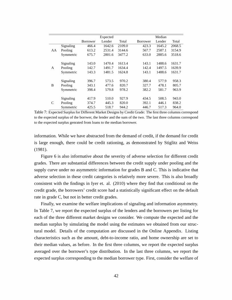
Expected Median

Borrower Lender Total Borrower Lender Total

Signaling 466.4 1642.6 2109.0 423.3 1645.2 2068.5

AA Pooling 613.2 2531.4 3144.6 567.7 2587.1 3154.9

Symmetric 675.7 2801.6 3477.2 633.0 2885.6 3518.6

Signaling 143.0 1470.4 1613.4 143.1 1488.6 1631.7

A Pooling 142.7 1491.7 1634.4 142.4 1497.5 1639.9

Symmetric 143.3 1481.5 1624.8 143.1 1488.6 1631.7

Signaling 396.7 573.5 970.2 380.4 577.9 958.3

B Pooling 343.1 477.6 820.7 327.7 478.1 805.7

Symmetric 398.4 579.8 978.2 382.2 581.7 963.9

Signaling 417.9 510.0 927.9 434.5 508.5 943.0

C Pooling 374.7 445.3 820.0 392.1 446.1 838.2

Symmetric 425.5 518.7 944.2 446.7 517.3 964.0

Table 7: Expected Surplus for Different Market Designs by Credit Grade: The first three columns correspond

to the expected surplus of the borrwer, the lender and the sum of the two. The last three columns correspond

to the expected surplus genrated from loans to the median borrower.

information. While we have abstracted from the demand of credit, if the demand for credit

is large enough, there could be credit rationing, as demonstrated by Stiglitz and Weiss

(1981).

Figure 6 is also informative about the severity of adverse selection for different credit

grades. There are substantial differences between the credit supply under pooling and the

supply curve under no asymmetric information for grades B and C. This is indicative that

adverse selection in these credit categories is relatively more severe. This is also broadly

consistent with the findings in Iyer et. al. (2010) where they find that conditional on the

credit grade, the borrowers’ credit score had a statistically significant effect on the default

rate in grade C, but not in better credit grades.

Finally, we examine the welfare implications of signaling and information asymmetry.

In Table 7, we report the expected surplus of the lenders and the borrowers per listing for

each of the three different market designs we consider. We compute the expected and the

median surplus by simulating the model using the estimates we obtained from our struc-

tural model. Details of the computation are discussed in the Online Appendix. Listing

characteristics such as the amount, debt-to-income ratio, and home ownership are set to

their median values, as before. In the first three columns, we report the expected surplus

averaged over the borrower’s type distribution. In the last three columns, we report the

expected surplus corresponding to the median borrower type. First, consider the welfare of

42

the borrowers reported in the first column. Comparing the borrower welfare under pool-

ing and under no asymmetric information, we find that the welfare loss from information

asymmetry is relatively modest in credit grade A ($142.7 under pooling and $143.3 un-

der no asymmetric information) while the welfare loss is relatively more severe in credit

grades B and C ($343.1 under pooling $398.4 under no asymmetric information for credit

grade B, and $374.7 under pooling and $425.5 under no asymmetric information for credit

grade C), confirming our earlier remark that adverse selection is more serious in credit

grades B and C. Comparing these numbers to the welfare results under signaling, we find

that welfare improves relative to pooling in all credit grades except for credit grade AA.

In particular, for credit grades B and C, signaling restores most of the welfare loss caused

by adverse selection. For credit grade AA, the borrower welfare under pooling is higher

than the borrower welfare under signaling. This happens because the surplus that must be

burned (i.e., the transactions that must be foregone by submitting a lower reserve interest

rate under signaling) in order to maintain a separating equilibrium is sufficiently costly.

This off-sets any benefits gained by reducing information asymmetry between the lenders

and the borrowers. Note that in general, it is not possible to Pareto-rank equilibrium under

pooling and signaling.

Second, consider the welfare of the lenders reported in the second column. Comparing

the welfare of the lenders under pooling and under no asymmetric information, we find

that welfare decreases considerably under pooling in all credit grades except for credit

grade A, where welfare of the lenders is slightly higher under pooling. Similar to what we

found for the case of borrowers, we find that signaling improves welfare in credit grades

B and C, but not in credit grade AA (and A). Again, the reason for this is that for credit

grade AA, there is a net decrease in the listings that are funded as a result of low reserve

rates. This is in contrast to credit grades B and C where the increased credit supply from

reducing information asymmetry outweighs the reduction in transactions that result from

lower reserve interest rates.

Finally, the third column of Table 7 is informative about the cost of adverse selection,

as well as the extent to which welfare can be restored through signaling. Comparing the

total surplus under pooling and no asymmetric information, we find that the cost of adverse

selection can be quite large, with a 16% ($157.5) decrease in total surplus for credit grade

B and a 13% ($124.2) decrease in total surplus for credit grade C. We also find that in some

instances, signaling can restore a large fraction of the potential welfare loss from adverse

selection, with 95% and 87% of the welfare loss avoided through signaling in credit grades

43

B and C.

9 Robustness to Rational Expectations

An important assumption we have made all along is that lenders have rational expectations.

While rational expectation is a strong assumption, note that our baseline model already

captures simple deviations from rational expectations. For example if all of the lenders are

optimistic (or pessimistic) by the same amount, then optimism will be captured in the mean

of ε0j .40 Hence, our baseline specification already captures lender optimism (or pessimism)

albeit in a reduced form manner. Moreover, we let the mean of the outside option to be time

varying in our baseline results, allowing for the optimism of the lenders to evolve over time.

Similarly, our model also captures aggregate trends that may result from lender learning or

recalibration of expectations.41

In order to better understand how lenders form beliefs and how they interact with

other financial markets, we estimated an alternative specification with more structure on

the lenders’ beliefs. In particular, we estimated a model where the beliefs of the lenders are

given by

µ = µRE + ρ0 + ρ1µS&P

σ2 = σ2RE × exp(ν1σ2S&P ),

where µRE and σ2RE are the mean and variance of the realized loan return and µS&P and

σ2S&P are the weekly mean and the volatility index of the S&P 500 and ρ0, ρ1 and ν1

are parameters to be estimated. The mean of ε0j is set to zero, instead. Our estimates

(full results are reported in the Online Appendix) of ρ1 and v1 are quite close to zero,

implying that including the stock market performance does not improve much on rational

expectations. Figure 7 plots the counterfactual credit supply curve from this specification.

The supply curves are qualitatively similar to the baseline results in Figure 6.

40Adding a constant term, κ, to the rational expectations mean is equivalent to adding 50κ to the mean of

ε0j and subtracting 50κ and 150κ from c100 and c200.41Our model is obviously not rich enough to capture individual learning, however. It can only capture

aggregate trends that reflect a better informed pool of lenders.

44

Figure 7: The Credit Supply Curve for the Borrower of the Median Type. See Figure 6 for descrip-

tion.

10 Conclusion

In this paper, we study how signaling can restore some of the inefficiencies arising from

adverse selection using data from an online peer-to-peer lending market, Prosper.com. We

first provide some evidence showing that the reserve interest rate posted by potential bor-

rowers work as a signaling device. Based on this evidence, we then develop and estimate

a structural model of borrowers and lenders. In our counterfactual, we compare the credit

supply curve and welfare under three different market designs: a market with signaling, a

market without signaling, and a market with no asymmetric information. We find that in

one of the credit grades, signaling exacerbates the welfare cost of adverse selection, but

we also find that signaling can restore much of the welfare losses that result from adverse

selection in other credit grades.

Our paper is the first structural analysis of signaling in industrial organization to the best

of our knowledge, and it is also the first attempt at estimating the credit supply curve, as far

as we are aware. We also believe that the methods developed in the paper can be applied

to other settings in which signaling is important (e.g., auctions and reservation price). For

future research, we think that it is important to study other types of credit markets in order

to understand more fully the costs of adverse selection and the benefits of signaling.

A Appendix

A.1 Proof of Proposition 1

We provide a proof of Proposition 1. We do so by first proving the following lemma.

45

Lemma 1 ∂∂ϕV1(r, ϕ) is non-increasing in r.

Proof. The proof is by induction. We first show that ∂∂r∂ϕ

VT (r, ϕ) ≤ 0, ∂∂rVT (r, ϕ) ≤ 0,

and D′(ϕ) ≤ β ∂∂ϕVT (r, ϕ) < 0. We then show that if ∂

∂r∂ϕVτ (r, ϕ) ≤ 0 and D′(ϕ) ≤

∂∂ϕVτ (r, ϕ) < 0 for some τ ≤ T , then the same conditions hold for τ − 1. First, for t = T ,

∂

∂ϕVT (r, ϕ) =

∂

∂ϕ

∫max{uT (r) + εT , D(ϕ)}dFεT (εT ) = D′(ϕ) PrT (r, ϕ) ,

where PrT (r, ϕ) = Pr(uT (r) + εT < D(ϕ)). It is easy to see that D′(ϕ) ≤ ∂∂ϕVT (r, ϕ) <

β ∂∂ϕVT (r, ϕ) < 0 because D′(ϕ) < 0, by assumption and Pr (uT (r) + εT < D(ϕ)) ∈

(0, 1). Also, note that ∂∂ruT (r) < 0 implies ∂

∂rPr (uT (r) + εT < D(ϕ)) > 0, which means

that ∂∂r∂ϕ

VT (r, ϕ) ≤ 0. It is also easy to see that ∂∂rVT (r, ϕ) < 0.

Now, assume ∂∂r∂ϕ

Vt+1(r, ϕ) ≤ 0, ∂∂rVt+1(r, ϕ) ≤ 0, and D′(ϕ) ≤ β ∂

∂ϕVt+1(r, ϕ) < 0

for some t. Then,

∂

∂ϕVt(r, ϕ) =

∂

∂ϕ

∫max{ut(r) + εt + βVt+1(r, ϕ), D(ϕ)}dFεt(εt)

=∂

∂ϕβVt+1(r, ϕ)(1− Prt (r, ϕ)) +D′(ϕ) Prt (r, ϕ) ≥ D′(ϕ),

where Prt (r, ϕ) = Pr(ut(r) + εt + βVt+1(r, ϕ) < D(ϕ)). The last inequality holds since∂∂ϕVt+1(r, ϕ) ≥ D′(ϕ). Again, it is easy to see ∂

∂ϕVt(r, ϕ) < 0, and ∂

∂rVt(r, ϕ) ≤ 0. To see

that ∂∂r∂ϕ

Vt(r, ϕ) ≤ 0, note that

∂

∂r∂ϕVt(r, ϕ) =

∂

∂r

[∂

∂ϕβVt+1(r, ϕ)(1− Prt (r, ϕ)) +D′(ϕ) Prt (r, ϕ)

]=

∂2

∂r∂ϕβVt+1(r, ϕ)(1− Prt (r, ϕ)) +

∂

∂rPrt (r, ϕ)× (D′(ϕ)− ∂

∂ϕβVt+1(r, ϕ)) ≤ 0.

By induction we conclude that ∂∂r∂ϕ

V1(r, ϕ) ≤ 0.

Proposition 1 If ∂∂s

Pr(s) > 0 and F (r|s) FOSD F (r|s′) for s′ > s, then we have SCP,

i.e.,

∂2

∂s∂ϕV0(s, ϕ) =

∂2

∂s∂ϕ

[Pr(s)

∫V1(r, ϕ)f(r|s)dr + (1− Pr(s))λ(ϕ)

]< 0.

Proof. First, let us consider the second term. Note that ∂2

∂s∂ϕ(1 − Pr(s))λ(ϕ) =

−Pr′(s)λ′(ϕ) < 0. This is because Pr′(s) > 0 and λ′(ϕ) > 0 by assumption. Second,

46

we consider the first term. Note that for s0 < s1, F (r|s1) first-order stochastically dom-

inates F (r|s0). Hence if ∂∂ϕV1(r, ϕ) is non-increasing in r, then

∫∂∂ϕV1(r, ϕ)dF (r|s0) ≥∫

∂∂ϕV1(r, ϕ)dF (r|s1) for any s0 and s1 s.t. s0 < s1. This implies that ∂

∂s∂ϕPr(s)

∫V1(r, ϕ)dF (r|s) ≤

0. Thus, we complete the proof.

A.2 Proof of Proposition 3

In this Appendix, we provide a proof of identification of Fϕ|X , Fε|X , and λ(ϕ). We first

note that we can normalize one of the constants in ut without loss of generality: Hence

we set dT = 0.42 Also, we can normalize the location of Fϕ|X at one point: Hence, we

set F−1ϕ|X∗(α∗) = 0 for some α∗ ∈ (0, 1) and X∗.43 In what follows, we consider the case

when there is no pooling. The Online Appendix contains the proof for the case when there

is partial pooling.

Consider the repayment decision of the borrower with ϕα∗ = F−1ϕ|X∗(α∗) at period t =

T . The borrower’s problem is as follows:{repay: if − (r × x∗amt) + εT ≥ −F−1ϕ|X∗(α∗) = 0

default: otherwise,

where x∗amt is an element of X∗. This is simply a binary threshold-crossing model; hence

using variation in r, we can nonparametrically identify the conditional distribution of εT

given X∗, i.e., Fε|X∗ . Once Fε|X∗ is identified, we can identify F−1ϕ|X∗(α) for all α given

X∗ by conditioning the sample on the α-quantile of s given X∗ (i.e., samples with s =

F−1s|X∗(α)).44 This is because F−1ϕ|X∗(α) is just a constant term in the binary threshold-

crossing model where the distribution of εT given X∗ has already been identified.

Now consider the t = T − 1 period problem with X = X∗:{repay: if − (r × x∗amt) + dT−1 + βVT (r, F−1ϕ|X∗(α)) + εT−1 ≥ −F−1ϕ|X∗(α)

default: otherwise,

where VT (r, F−1ϕ|X∗(α)) and F−1ϕ|X∗(α) have already identified. Similarly as before, we can

42If we set d̃t = dt + κ (∀t) ε̃t = εt − κ (∀t), it will be observationally equivalent to dt, Fε|X .43Given thatD(ϕ) = −ϕ, if we set ε̃t = εt+κ (∀t), F̃ϕ|X(h) = Fϕ|X(h+κ), d̃T = dT , and d̃t = dt−βκ

(t ∈ {1, ..., T − 1}) and λ̃(ϕ) = λ(ϕ) + βκ, it will be observationally equivalent to εt, dt, Fϕ|X , and λ.

This normalization is convenient for proving identification, but we use an equivalent normalization (i.e.,

Med[εt|X] = const.) for our estimation.44Here, we are using the fact that ϕ ⊥ ε|X∗.

47

nonparametrically identify the distribution of (εT−1+dT−1) and the value of β using varia-

tion in r, given that this is a simple binary threshold crossing model. It should be clear that

{εt + dt}t≤T−2 can also be identified by looking at the borrower’s period t problem and the

associated default probability.

Now, we discuss how to identify λ(ϕ). Rearranging the borrower’s FOC in equation

(7) evaluated at X = X∗ and solving for λ(ϕ), we obtain

λ(ϕ) =

∫V1(r, ϕ;X∗)f(r|s;X∗)dr+

Pr(s;X∗)∂∂s

Pr(s;X∗)

∫V1(r, ϕ;X∗)

∂

∂sf(r|s;X∗)dr, (2)

where we have made the dependence on X∗ explicit. Note that all the terms on the right

hand side are identified. First, V1 is identified given that Fε|X∗ , Fϕ|X∗ , and β have already

been identified. Also, we know that borrowers of type ϕ submit a reserve rate equal to

s(ϕ;X∗) = F−1s|X∗(Fϕ|X∗(ϕ)). Then evaluating Pr(s;X∗) and f(r|s;X∗) – which are both

directly observed in the data – at s(ϕ;X∗), we can identify the right-hand side of the

equation. Hence the previous equation identifies λ(ϕ).

Lastly, we show that Fϕ|X and Fε|X are identified for any X . To see that Fϕ|X and

Fε|X are identified for any X , note that it is enough to identify Fϕ|X(0) – if Fϕ|X(0) is

identified, we can follow the same steps as above to identify Fϕ|X and Fε|X . In order

to see that Fϕ|X(0) is identified, consider a given profile, (F ∗ε|X , F∗ϕ|X , λ

∗, d∗t ). Note that

the set of profiles that are observationally equivalent to (F ∗ε|X , F∗ϕ|X , λ

∗, d∗t ) are given by

{(Fε|X , Fϕ|X , λ, dt) : Fε|X(h) = F ∗ε|X(h − κ), Fϕ|X(h) = F ∗ϕ|X(h + κ), dT = d∗T , dt =

d∗t − βκ (t < T ), λ(ϕ) = λ∗(ϕ) + βκ}. Given that we have already identified λ(ϕ), we

can identify Fϕ|X(0). This concludes the proof of identification when there is no pooling.

In the Online Appendix we also discuss the case when there is pooling at s = 36%.

References

[1] Ackerberg, Daniel, “Advertising, Learning, and Consumer Choice in Experience

Good Markets: A Structural Empirical Examination”, International Economic Re-

view, Vol. 44, No. 3, August 2003, pp. 1007-1040

[2] Adams, William, Liran Einav, Jonathan Levin, “Liquidity Constraints and Imperfect

Information in Subprime Lending,” American Economic Review, Vol. 99(1), 2009,

pp. 49–84.

48

[3] Akerlof, George A., “The Market for “Lemons”: Quality Uncertainty and the Market

Mechanism,” Quarterly Journal of Economics, Vol. 84(3), 1970, pp. 488-500.

[4] Arnold, Lutz and John Riley, “On the Possibility of Credit Rationing in the Stiglitz-

Weiss Model,” American Economic Review, Vol. 99, No. 5 (2009), pp. 2012-2021

[5] Ausubel, Larry, “Adverse Selection in the Credit Card Market,” mimeo, 1999.

[6] Berger, Allen N. and Gregory F. Udell, “Some Evidence on the Empirical Significance

of Credit Rationing,” Journal of Political Economy, Vol. 100 (5), 1992, pp. 1047-

1077.

[7] Cai, Hongbin, John Riley, and Lixin Ye, “Reserve Price Signaling,” Journal of Eco-

nomic Theory, Vol. 135, 2007, pp. 253 – 268.

[8] Cohen, Alma and Liran Einav, “Estimating Risk Preferences from Deductible

Choice,” American Economic Review, Vol. 97(3), 2007, pp. 745-788.

[9] Einav, Liran, Amy Finkelstein and Jonathan Levin, “Beyond Testing: Empirical Mod-

els of Insurance Markets,” Annual Review of Economics, 2010, pp. 311-36.

[10] Einav, Liran, Mark Jenkins, and Jonathan Levin, “Contract Pricing in Consumer

Credit Markets,” Econometrica, Vol. 80 (4), 2012, pp. 1387-432.

[11] Fang, Hanming, “Disentangling the College Wage Premium: Estimating a Model

with Endogenous Education Choices,” International Economic Review, Vol. 47 (4),

2006, pp. 1151-1185.

[12] Freedman, Seth and Ginger Jin, “Learning by Doing with Asymmetric Information:

Evidence from Prosper.com,” mimeo, 2010.

[13] Gallant, A. Ronald, and Douglas W. Nychka, “Semi-Nonparametric Maximum Like-

lihood Estimation,” Econometrica, Vol. 55(2), 1987, pp. 363-390.

[14] Gayle, George-Levi and Limor Golan, “Estimating a Dynamic Adverse-Selection

Model: Labour-Force Experience and the Changing Gender Earnings Gap 1968-97,”

Review of Economic Studies, Vol. 79 (1), 2012, pp. 227-67.

[15] Holt, Charles, and Susan Laury (2002) “Risk Aversion and Incentive Effects,” Amer-

ican Economic Review, 92(5), 1644-1655.

49

[16] Hörner, Johannes and Nicolas Sahuguet, “A War of Attrition with Endogenous Effort

Levels,” Economic Theory, Vol. 47, 2011, pp.1-27.

[17] Hungerford, Thomas and Gary Solon, “Sheepskin Effects in the Returns to Educa-

tion,” Review of Economics and Statistics, Vol. 69 (1), 1987, pp. 175-178.

[18] Iyer, Rajkamal, Asim Ijaz Khwaja, Erzo F. P. Luttmer, and Kelly Shue, “Inferring As-

set Quality: Determining Borrower Creditworthiness in Peer-to-Peer Lending Mar-

kets,” mimeo, 2010.

[19] Jullien, Bruno and Thomas Mariotti, “Auction and the Informed Seller Problem,”

Games and Economic Behavior, Vol. 56(2), 2006, pp. 225-58.

[20] Karlan, Dean and Jonathan Zinman, “Observing Unobservables: Identifying Infor-

mation Asymmetries With a Consumer Credit Field Experiment,” Econometrica, Vol.

77(6), 2009, pp. 1993-2008.

[21] Kim, Kyoo il, “Semiparametric Estimation of Signaling Games and Equilibrium Re-

finement,” mimeo, 2012

[22] Mailath, George J., “Incentive Compatibility in Signaling Games with a Continuum

of Types,” Econometrica, Vol. 55(6), 1987, pp. 1349-1365.

[23] Mas-Colell, Andreu, Michael Whinston and Jerry Green, Microeconomic Theory, Ox-

ford University Press, 1995.

[24] Mazkin, Rosa “Nonparametric and Distribution-Free Estimation of the Binary

Threshold Crossing and the Binary Choice Models,” Econometrica, Vol. 60, 1992,

239-270.

[25] Milgrom, Paul and John Roberts, “Limit Pricing and Entry under Incomplete Infor-

mation: An Equilibrium Analysis,” Econometrica, Vol. 50 (2), 1982, pp. 443-459.

[26] Milgrom, Paul and John Roberts, “Price and Advertising Signals of Product Quality,”

Journal of Political Economy, Vol. 94 (4), 1986, pp. 796-821.

[27] Morris, Stephen and Hyun Song Shin, “Contagious Adverse Selection,” American

Economic Journal: Macroeconomics, Vol. 4, 2012, pp. 1-21.

50

[28] Paravisini, Daniel, Veronica Rappoport and Enrichetta Ravina “Risk Aversion and

Wealth: Evidence from Person-to-Person Lending Portfolios,” mimeo, 2013.

[29] Powell, James, “Censored Regression Quantiles,” Journal of Econometrics, Vol. 32,

1986, pp. 143-55.

[30] Ravina, Enrichetta, “Love & Loans: The Effect of Beauty and Personal Characteris-

tics in Credit Markets,” mimeo, 2008.

[31] Rigbi, Oren, “The Effects of Usury Laws: Evidence from the Online Loan Market,”

forthcoming in Review of Economics and Statistics, 2011.

[32] Roberts, James, “Unobserved Heterogeneity and Reserve Prices in Auctions,” RAND

Journal of Economics, forthcoming.

[33] Spence, Michael, “Job Market Signaling,” Quarterly Journal of Economics, Vol.

87(3), 1973, pp. 355-374.

[34] Stiglitz, Joseph E., and Andrew Weiss, “Credit Rationing in Markets with Imperfect

Information,” American Economic Review, Vol. 71(3), 1981, pp. 393-410.

51