Signal Processing: Image Communication - …vision.eng.shizuoka.ac.jp/pubs/pdfs/Yi_SPIC_2014.pdf726 Y. Zhang et al. / Signal Processing: Image Communication 29 (2014) 725–747 type

Contents lists available at ScienceDirect

Signal Processing: Image Communication

Signal Processing: Image Communication 29 (2014) 725–747

http://d0923-59

n Corr

journal homepage: www.elsevier.com/locate/image

C-DIIVINE: No-reference image quality assessment basedon local magnitude and phase statistics of natural scenes

Yi Zhang a,n, Anush K. Moorthy b, Damon M. Chandler a, Alan C. Bovik b

a School of Electrical and Computer Engineering, Oklahoma State University, Stillwater, OK 74078, USAb Department of Electrical and Computer Engineering, The University of Texas at Austin, Austin, TX 78712, USA

a r t i c l e i n f o

Article history:Received 26 September 2013Received in revised form15 January 2014Accepted 14 May 2014Available online 28 May 2014

Keywords:Image quality assessmentComplex wavelet transformComplex Gaussian scale mixtureRelative phase

x.doi.org/10.1016/j.image.2014.05.00465/& 2014 Elsevier B.V. All rights reserved.

esponding author.

a b s t r a c t

It is widely known that the wavelet coefficients of natural scenes possess certain statisticalregularities which can be affected by the presence of distortions. The DIIVINE (DistortionIdentification-based Image Verity and Integrity Evaluation) algorithm is a successfulno-reference image quality assessment (NR IQA) algorithm, which estimates quality basedon changes in these regularities. However, DIIVINE operates based on real-valued waveletcoefficients, whereas the visual appearance of an image can be strongly determined byboth the magnitude and phase information.

In this paper, we present a complex extension of the DIIVINE algorithm (calledC-DIIVINE), which blindly assesses image quality based on the complex Gaussian scalemixture model corresponding to the complex version of the steerable pyramid wavelettransform. Specifically, we applied three commonly used distribution models to fit thestatistics of the wavelet coefficients: (1) the complex generalized Gaussian distribution isused to model the wavelet coefficient magnitudes, (2) the generalized Gaussian distribu-tion is used to model the coefficients' relative magnitudes, and (3) the wrapped Cauchydistribution is used to model the coefficients' relative phases. All these distributions havecharacteristic shapes that are consistent across different natural images but changesignificantly in the presence of distortions. We also employ the complex waveletstructural similarity index to measure degradation of the correlations across image scales,which serves as an important indicator of the subbands' energy distribution and the lossof alignment of local spectral components contributing to image structure. Experimentalresults show that these complex extensions allow C-DIIVINE to yield a substantialimprovement in predictive performance as compared to its predecessor, and highlycompetitive performance relative to other recent no-reference algorithms.

& 2014 Elsevier B.V. All rights reserved.

1. Introduction

A crucial task for any system that processes images forhuman viewing is the ability to assess the quality of eachimage in a manner that is consistent with human judg-ments of quality. To address this need, numerous algo-rithms for image quality assessment (IQA) have beendeveloped and refined over the past several decades using a

wide variety of image-modeling techniques. IQA algorithmshave been successfully used in applications such as image andvideo coding (e.g., [1–4]); unequal error protection (e.g., [5]);image synthesis (e.g., [6,7]); and in numerous other areas(e.g., [8–11]).

The vast majority of IQA algorithms are so-called full-reference algorithms, which take as input both a distortedimage and a reference image, and yield as output anestimate of the quality difference between the two images.The simplest approach to full-reference (FR) IQA is tomeasure local pixelwise differences, then collapse these

www.sciencedirect.com/science/journal/09235965

www.elsevier.com/locate/image

http://dx.doi.org/10.1016/j.image.2014.05.004



http://crossmark.crossref.org/dialog/?doi=10.1016/j.image.2014.05.004&domain=pdf




1 In this paper, we consider natural images to be photographicimages containing subject matter that may occur during normal photopicor scotopic viewing conditions.

Y. Zhang et al. / Signal Processing: Image Communication 29 (2014) 725–747726

local measurements into a scalar which represents theoverall quality difference; e.g., the mean-squared error(MSE) or peak signal-to-noise ratio (PSNR). More sophis-ticated FR IQA methods have employed a wide variety ofapproaches ranging from estimating quality differencesbased on weighted MSE/PSNR variants (often measured indifferent domains; e.g., [12]), to estimating quality differ-ences based on models of the human visual system (e.g.,[13–19,3,20–22,4,23–26]), and estimating quality based onvarious feature-extraction-based or information-theoretic-based approaches (e.g., [27–33]).

FR IQA provides a useful and effective way to evaluatequality differences; however, in many cases, the referenceimage or even partial information about the referenceimage is not available (partial information may be usedfor reduced-reference IQA; see, e.g., [34–36]). Althoughhumans can often effortlessly judge the quality of adistorted image in the absence of a reference image, theno-reference QA task has proven to be quite challengingfrom a modeling perspective. No-reference IQA modelsattempt to perform this task, i.e., to estimate the quality ofa distorted image without a corresponding referenceimage. The advantages of a no-reference (NR) approachare numerous: in an IP streaming application, for example,only the compressed (distorted) image is received, andthus quality judgments must be made without access tothe reference. Similarly, in digital photography, it is oftendesirable to determine the quality of the captured imagerelative to the original scene; this scenario requires a NRapproach because the original scene cannot be provided tothe IQA method.

The vast majority of NR IQA algorithms attempt todetect specific types of distortion such as blurring, block-ing, ringing, or various forms of noise (e.g., [37–42]).For example, algorithms for sharpness/blurriness estima-tion have been shown to perform well in NR IQA ofblurred images. The vast majority of sharpness/blurrinessestimators operate under the assumption that the app-earance of edges is affected by blur, and accordinglythese methods estimate sharpness/blurriness by usingvarious edge-appearance models (e.g., [43–45]). Othermethods have used spectral information to estimatesharpness (e.g., [46,47]), whereas more recent hybridapproaches employ a combination of edge-based andtransform-based methods. NR IQA algorithms have alsobeen designed specifically for JPEG or JPEG2000 com-pression artifacts (e.g., [37–39]). Such JPEG-specificalgorithms generally employ detectors for blocking andblurring, which are often combined with measures ofvisual masking to estimate the visibility of each of theseartifacts, and thereby estimate quality. Similar NR IQAalgorithms have been designed specifically for JPEG2000ringing, blurring, and aliasing artifacts (e.g., [40,37–39]).Some NR algorithms have employed combinations of theseaforementioned measures, supplemented with noise mea-sures and/or other measures for degradations of other visualfeatures (e.g., [41,48,42]).

Other NR IQA algorithms take a more distortion-agnostic approach. For example, a training/learning-basedapproach has been recently developed which extractsGabor-filter-based features from local image patches and

then learns the mapping from the quantized feature spaceto image quality by using a visual-codebook-based method[49,50]. Other approaches estimate image quality based onthe extent to which the statistical properties of thedistorted image deviate from those of natural images.1

Natural scenes have been studied extensively over the lasttwo decades and these studies have revealed that suchimages have a large number of statistical regularities (e.g.,[51–53]). Distortions can lead to deviations in thesestatistical regularities, and thus it is possible to estimatequality by quantifying these deviations. For example, in[54], the authors developed a NR IQA algorithm whichestimates quality by using the Renyi entropy to measuredeviations in anisotropy along various orientations. In [55],the authors developed a NR IQA algorithm (BLIINDS)which estimates quality based on deviations in DCTstatistics (e.g., changes in the characteristic shape/symme-try of DCT coefficient histograms). Most recently, a spatial-domain-based NR IQA model was proposed in [56], whichuses scene statistics of locally normalized luminancecoefficients to quantify possible losses of ‘naturalness’ inthe image due to the presence of distortion, leading to aholistic measure of quality.

One particular NR IQA algorithm, DIIVINE (DistortionIdentification-based Image Verity and INtegrity Evalua-tion) [57], — the algorithm which the method proposed inthis paper extends — employs a two-stage framework forestimating quality based on natural-scene statistics. DII-VINE estimates quality by using statistical features whichare generally consistent across reference images, butwhich change in the presence of distortion. In this way,it is possible to compute the extent to which the statisticalfeatures in the distorted image deviate from theseexpected natural statistical features, and then to use thesedeviations as proxy measures of quality degradations.

In [57], a steerable pyramid decomposition is firstapplied to obtain a multi-scale, multi-orientation repre-sentation of the distorted image [58]. The real-valuedcoefficients are then processed through a divisive normal-ization operation. As demonstrated in [57], the histogramsof these normalized coefficients exhibit Gaussian-likeprofiles which are generally consistent across naturalimages. The coefficients were also shown to exhibit strongcorrelations between spatially co-located/neighboringcoefficients from different scales and orientations. Fromthe distorted image, 88 statistical features are measured in[57]. These 88 statistical features are then used to estimatequality via the following two stages: The first stage per-forms distortion identification. In this stage, the statisticalfeatures extracted from the distorted image are fed toa classifier to estimate the probability that the imageis afflicted by one of the multiple distortion types.The second stage performs distortion-specific qualityassessment. In this stage, the same statistical features areused to estimate the distortion-specific quality of theimage. Specifically, a regression model for each distortion

Y. Zhang et al. / Signal Processing: Image Communication 29 (2014) 725–747 727

type is used to map the statistical features to qualityestimates based on the probabilities estimated in the firststage. DIIVINE has been shown to perform remarkably wellin estimating quality. It is one of the best-performing NRIQA methods available, its ideas have given rise to a relatedpixel-based NR IQA method [56], and it has been shown tobe competitive with top-performing FR IQA algorithms.

In this paper, we present an extended version of theDIIVINE algorithm which operates based on the localmagnitude and phase statistics of complex wavelet imagecoefficients. Over the last three decades, considerableinsights into the properties of visual systems have beengained by considering the statistics of natural scenes (e.g.,[51,59,60,52,53,61]). These approaches have demonstratedthat many basic properties of the early visual system (bothselectivity and tiling of visual neurons) and properties ofvisual perception can be linked to the statistics of naturalscenes. Natural scenes exhibit a characteristic magnitudespectrum which generally follows a f �α trend, where fdenotes radial spatial frequency [51]. Estimates of the para-meter α for any given scene population typically vary from0.7 to 1.5 with averages in the range of approximately 1.1[59,62]. Natural scenes also posses a coherent phase struc-ture which has been shown to be the primary contributor toan image's phenomenal appearance. Oppenheim and Lim[63] first demonstrated this fact by synthesizing an imagefrom the magnitude spectrum of one image and phasespectrum of another; the resulting image appeared muchmore similar to the image whose phase structure was used.Thomson, Foster, and Summers [64] have demonstrated thatrandomization or quantization of this phase structureseverely impacts the semblance of an image. Bex andMakous [65] have shown that randomizing a natural image'sphase structure at a particular spatial scale decreases detec-tion and contrast-matching performance by the sameamount as removing the spatial scale altogether. In addition,Geisler et al. [66] have demonstrated that human perfor-mance in detecting contours can be predicted via amodel based on the edge co-occurrence statistics of naturalimages.

Yet, although the phase spectrum of full-sized imageshas long been argued to be much more perceptuallyimportant than the magnitude spectrum, the individualcontributions of magnitude and phase have been shown tovary according to scale. Morgan et al. [67] demonstratedthat for larger image patches, the perceived image struc-ture is well described by the phase spectrum, whereas forsmall image patches, the magnitude spectrum dominates.More recently, Field and Chandler [68] argued that thescale-dependent importance of magnitude vs. phase is dueto the sparse structure of images and the nature of theinformation in small patches. Specifically, most smallimage patches contain blank regions, single edges, or bitsof texture. The power spectra for these small patches can bequite informative regarding which of these classes are present.However, larger image patches will typically contain a sig-nificant number of edges as well as textures and blankregions. For these larger patches, the phase spectrum isdetermined by the relative combination and positions of thesefeatures, and thus the phase spectrum will begin to play alarger role in determining the image's appearance.

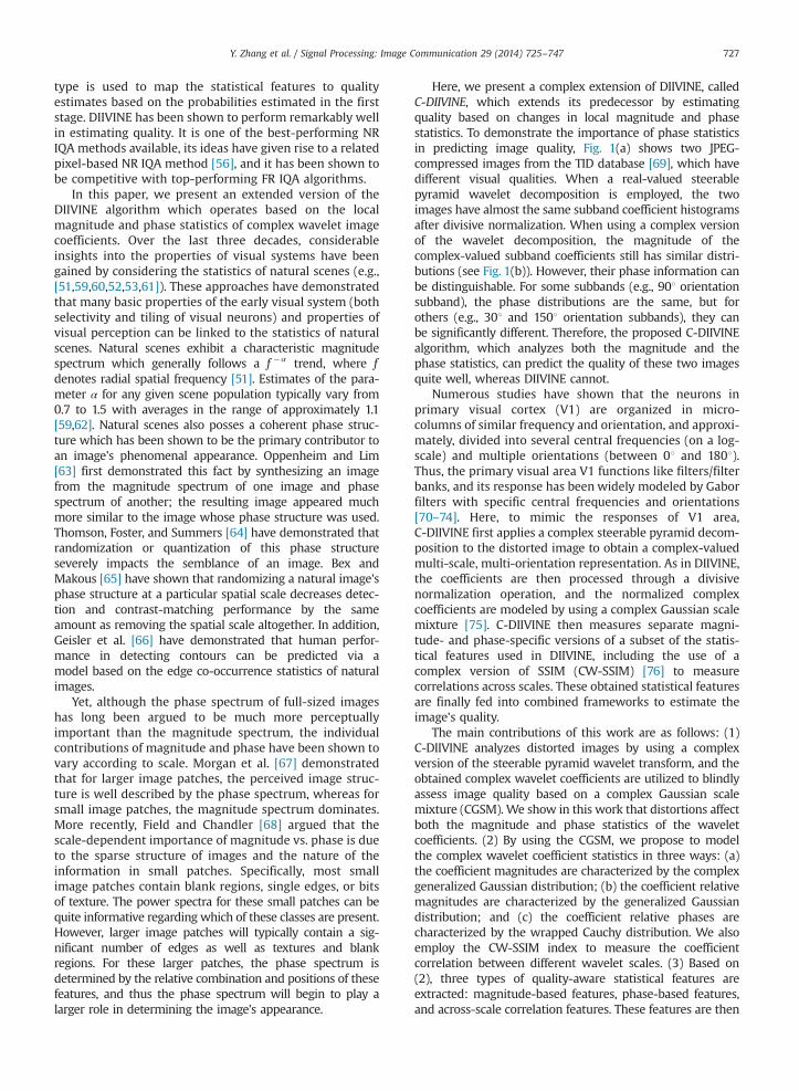
Here, we present a complex extension of DIIVINE, calledC-DIIVINE, which extends its predecessor by estimatingquality based on changes in local magnitude and phasestatistics. To demonstrate the importance of phase statisticsin predicting image quality, Fig. 1(a) shows two JPEG-compressed images from the TID database [69], which havedifferent visual qualities. When a real-valued steerablepyramid wavelet decomposition is employed, the twoimages have almost the same subband coefficient histogramsafter divisive normalization. When using a complex versionof the wavelet decomposition, the magnitude of thecomplex-valued subband coefficients still has similar distri-butions (see Fig. 1(b)). However, their phase information canbe distinguishable. For some subbands (e.g., 901 orientationsubband), the phase distributions are the same, but forothers (e.g., 301 and 1501 orientation subbands), they canbe significantly different. Therefore, the proposed C-DIIVINEalgorithm, which analyzes both the magnitude and thephase statistics, can predict the quality of these two imagesquite well, whereas DIIVINE cannot.

Numerous studies have shown that the neurons inprimary visual cortex (V1) are organized in micro-columns of similar frequency and orientation, and approxi-mately, divided into several central frequencies (on a log-scale) and multiple orientations (between 01 and 1801).Thus, the primary visual area V1 functions like filters/filterbanks, and its response has been widely modeled by Gaborfilters with specific central frequencies and orientations[70–74]. Here, to mimic the responses of V1 area,C-DIIVINE first applies a complex steerable pyramid decom-position to the distorted image to obtain a complex-valuedmulti-scale, multi-orientation representation. As in DIIVINE,the coefficients are then processed through a divisivenormalization operation, and the normalized complexcoefficients are modeled by using a complex Gaussian scalemixture [75]. C-DIIVINE then measures separate magni-tude- and phase-specific versions of a subset of the statis-tical features used in DIIVINE, including the use of acomplex version of SSIM (CW-SSIM) [76] to measurecorrelations across scales. These obtained statistical featuresare finally fed into combined frameworks to estimate theimage's quality.

The main contributions of this work are as follows: (1)C-DIIVINE analyzes distorted images by using a complexversion of the steerable pyramid wavelet transform, and theobtained complex wavelet coefficients are utilized to blindlyassess image quality based on a complex Gaussian scalemixture (CGSM). We show in this work that distortions affectboth the magnitude and phase statistics of the waveletcoefficients. (2) By using the CGSM, we propose to modelthe complex wavelet coefficient statistics in three ways: (a)the coefficient magnitudes are characterized by the complexgeneralized Gaussian distribution; (b) the coefficient relativemagnitudes are characterized by the generalized Gaussiandistribution; and (c) the coefficient relative phases arecharacterized by the wrapped Cauchy distribution. We alsoemploy the CW-SSIM index to measure the coefficientcorrelation between different wavelet scales. (3) Based on(2), three types of quality-aware statistical features areextracted: magnitude-based features, phase-based features,and across-scale correlation features. These features are then

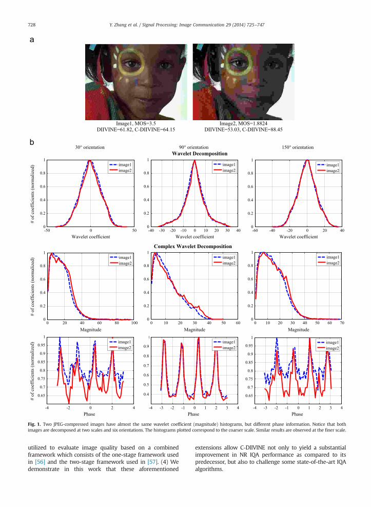
Image1, MOS=3.5 DIIVINE=61.82, C-DIIVINE=64.15

Image2, MOS=1.8824 DIIVINE=53.03, C-DIIVINE=88.45

30° orientation 90° orientation 150° orientation Wavelet Decomposition

Complex Wavelet Decomposition

-50 0 500

0.2

0.4

0.6

0.8

1

# of

coe

ffic

ient

s (no

rmal

ized

)

Wavelet coefficient

image1image2

-40 -30 -20 -10 0 10 20 30 400

0.2

0.4

0.6

0.8

1

Wavelet coefficient

image1image2

-60 -40 -20 0 20 400

0.2

0.4

0.6

0.8

1

Wavelet coefficient

image1image2

0 20 40 60 80 1000

0.2

0.4

0.6

0.8

1

# of

coe

ffic

ient

s (no

rmal

ized

)

Magnitude

image1image2

0 10 20 30 40 50 600

0.2

0.4

0.6

0.8

1

Magnitude

image1image2

0 10 20 30 40 50 60 700

0.2

0.4

0.6

0.8

1

Magnitude

image1image2

-4 -2 0 2 4

0.65

0.7

0.75

0.8

0.85

0.9

0.95

1

# of

coe

ffic

ient

s (no

rmal

ized

)

Phase

image1image2

-4 -3 -2 -1 0 1 2 3 4

0.4

0.5

0.6

0.7

0.8

0.9

1

Phase

image1image2

-4 -3 -2 -1 0 1 2 3 4

0.65

0.7

0.75

0.8

0.85

0.9

0.95

1

Phase

image1image2

Fig. 1. Two JPEG-compressed images have almost the same wavelet coefficient (magnitude) histograms, but different phase information. Notice that bothimages are decomposed at two scales and six orientations. The histograms plotted correspond to the coarser scale. Similar results are observed at the finer scale.


utilized to evaluate image quality based on a combinedframework which consists of the one-stage framework usedin [56] and the two-stage framework used in [57]. (4) Wedemonstrate in this work that these aforementioned

extensions allow C-DIIVINE not only to yield a substantialimprovement in NR IQA performance as compared to itspredecessor, but also to challenge some state-of-the-art IQAalgorithms.

SVM Training Training

Database

Test Image

Magnitude Statistics C-DIIVINE IQA Index Features/ Feature Pooling

Steerable Pyramid Complex Wavelet

Transform

Phase Statistics

Scale Correlation Statistics

Feature Extraction SVM Model

Image Quality

SVM Testing

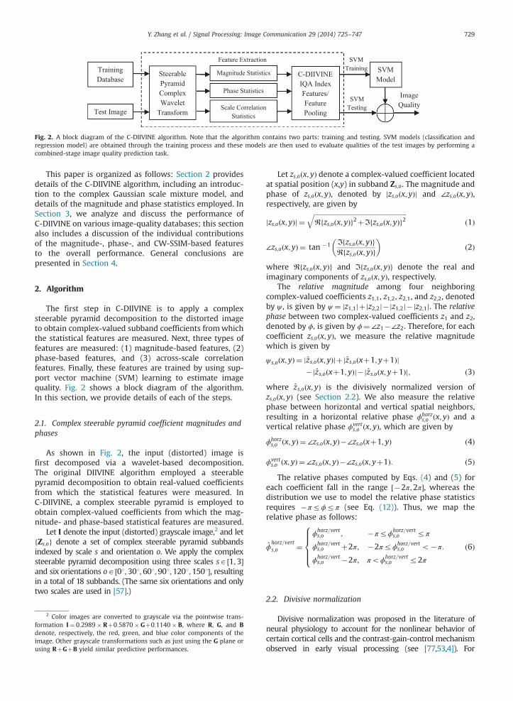
Fig. 2. A block diagram of the C-DIIVINE algorithm. Note that the algorithm contains two parts: training and testing. SVM models (classification andregression model) are obtained through the training process and these models are then used to evaluate qualities of the test images by performing acombined-stage image quality prediction task.


This paper is organized as follows: Section 2 providesdetails of the C-DIIVINE algorithm, including an introduc-tion to the complex Gaussian scale mixture model, anddetails of the magnitude and phase statistics employed. InSection 3, we analyze and discuss the performance ofC-DIIVINE on various image-quality databases; this sectionalso includes a discussion of the individual contributionsof the magnitude-, phase-, and CW-SSIM-based featuresto the overall performance. General conclusions arepresented in Section 4.

2. Algorithm

The first step in C-DIIVINE is to apply a complexsteerable pyramid decomposition to the distorted imageto obtain complex-valued subband coefficients fromwhichthe statistical features are measured. Next, three types offeatures are measured: (1) magnitude-based features, (2)phase-based features, and (3) across-scale correlationfeatures. Finally, these features are trained by using sup-port vector machine (SVM) learning to estimate imagequality. Fig. 2 shows a block diagram of the algorithm.In this section, we provide details of each of the steps.

2.1. Complex steerable pyramid coefficient magnitudes andphases

As shown in Fig. 2, the input (distorted) image isfirst decomposed via a wavelet-based decomposition.The original DIIVINE algorithm employed a steerablepyramid decomposition to obtain real-valued coefficientsfrom which the statistical features were measured. InC-DIIVINE, a complex steerable pyramid is employed toobtain complex-valued coefficients from which the mag-nitude- and phase-based statistical features are measured.

Let I denote the input (distorted) grayscale image,2 and letfZs;og denote a set of complex steerable pyramid subbandsindexed by scale s and orientation o. We apply the complexsteerable pyramid decomposition using three scales sA ½1;3�and six orientations oA ½01;301;601;901;1201;1501�, resultingin a total of 18 subbands. (The same six orientations and onlytwo scales are used in [57].)

2 Color images are converted to grayscale via the pointwise trans-formation I¼ 0:2989� Rþ0:5870� Gþ0:1140� B, where R, G, and Bdenote, respectively, the red, green, and blue color components of theimage. Other grayscale transformations such as just using the G plane orusing RþGþB yield similar predictive performances.

Let zs;oðx; yÞ denote a complex-valued coefficient locatedat spatial position (x,y) in subband Zs;o. The magnitude andphase of zs;oðx; yÞ, denoted by jzs;oðx; yÞj and ∠zs;oðx; yÞ,respectively, are given by

jzs;oðx; yÞj ¼ffiffiffiffiffiffiffiffiffiffiffiffiffiffiffiffiffiffiffiffiffiffiffiffiffiffiffiffiffiffiffiffiffiffiffiffiffiffiffiffiffiffiffiffiffiffiffiffiffiffiffiffiffiffiffiffiffiRfzs;oðx; yÞg2þIfzs;oðx; yÞg2

qð1Þ

∠zs;o x; yð Þ ¼ tan �1 Ifzs;oðx; yÞgRfzs;oðx; yÞg

� �ð2Þ

where Rfzs;oðx; yÞg and Ifzs;oðx; yÞg denote the real andimaginary components of zs;oðx; yÞ, respectively.

The relative magnitude among four neighboringcomplex-valued coefficients z1;1, z1;2, z2;1, and z2;2, denotedby ψ , is given by ψ ¼ jz1;1jþjz2;2j�jz1;2j�jz2;1j. The relativephase between two complex-valued coefficients z1 and z2,denoted by ϕ, is given by ϕ¼ ∠z1�∠z2. Therefore, for eachcoefficient zs;oðx; yÞ, we measure the relative magnitudewhich is given by

ψ s;oðx; yÞ ¼ jzs;oðx; yÞjþjzs;oðxþ1; yþ1Þj�jzs;oðxþ1; yÞj�jzs;oðx; yþ1Þj; ð3Þ

where zs;oðx; yÞ is the divisively normalized version ofzs;oðx; yÞ (see Section 2.2). We also measure the relativephase between horizontal and vertical spatial neighbors,resulting in a horizontal relative phase ϕhorz

s;o ðx; yÞ and avertical relative phase ϕvert

s;o ðx; yÞ, which are given by

ϕhorzs;o ðx; yÞ ¼∠zs;oðx; yÞ�∠zs;oðxþ1; yÞ ð4Þ

ϕverts;o ðx; yÞ ¼∠zs;oðx; yÞ�∠zs;oðx; yþ1Þ: ð5Þ

The relative phases computed by Eqs. (4) and (5) foreach coefficient fall in the range ½�2π;2π�, whereas thedistribution we use to model the relative phase statisticsrequires �πrϕrπ (see Eq. (12)). Thus, we map therelative phase as follows:

ϕhorz=verts;o ¼

ϕhorz=verts;o ; �πrϕhorz=vert

s;o rπ

ϕhorz=verts;o þ2π; �2πrϕhorz=vert

s;o o�π:

ϕhorz=verts;o �2π; πoϕhorz=vert

s;o r2π

8>>><>>>:

ð6Þ

2.2. Divisive normalization

Divisive normalization was proposed in the literature ofneural physiology to account for the nonlinear behavior ofcertain cortical cells and the contrast-gain-control mechanismobserved in early visual processing (see [77,53,4]). For


example, it has been shown in [78] that an additional localgain-control divisive normalization process allows for a morecomplete explanation of the striate cell responses wheninterpreted by the conventional linear/energy model, whichassumes that the simple cells in the striate cortex act like half-wave-rectified linear operators, and the complex cells act likeenergy mechanisms, constructed from linear subunits.In computational vision science, a long-standing view of thepurpose of early visual sensory processing is the increasedstatistical independence between neuronal responses. Thedivisive normalization process has been shown to successfullyreduce the statistical dependencies between subbands, pro-ducing approximately Gaussian marginal distributions for thewavelet coefficients [79], and this technique has been expli-citly used for RR IQA in [80].

We applied the same technique to the complex waveletcoefficients (following [57]). As demonstrated in [75], thereal and imaginary parts of the neighboring complexsubband coefficients can have the same scalar multiplierif either one follows the Gaussian scale mixture, and bydividing an estimated scalar multiplier (i.e., divisive nor-malization), the wavelet coefficient magnitudes can becharacterized by a complex generalized Gaussian distribu-tion (see Fig. 5). We show that distortions affect thehistogram shapes of these normalized magnitudes,whereas the natural images maintain almost the samemagnitude histogram profiles.

The divisively normalized version of each coefficient,denoted by zs;o, is obtained via

zs;o x; yð Þ ¼ zs;oðx; yÞffiffiffiffiffiffiffiffiffiffiffiffiffiffiffiffiffiffiffiffi1NP

TC�1Pall

Pq ; ð7Þ

whereffiffiffiffiffiffiffiffiffiffiffiffiffiffiffiffiffiffiffiffiffiffiffiffiffiffiffiffiffið1=NÞPTC�1

PallP

qis a real-valued scalar representing

the combined response of the normalization pool (neigh-boring coefficients). Note that, because

ffiffiffiffiffiffiffiffiffiffiffiffiffiffiffiffiffiffiffiffiffiffiffiffiffiffiffiffiffið1=NÞPTC�1

PallP

qis a

real-valued scalar, both Rfzs;oðx; yÞg and Ifzs;oðx; yÞg aredivided by this same value. Accordingly, the magnitudejzs;oðx; yÞj is affected by the divisive normalization, whereasthe phase ∠zs;oðx; yÞ (and thus the relative phase) is not.

The vector P in Eq. (7) is a 15-element vector consistingof the magnitudes of neighboring coefficients in space,scale, and orientation. Specifically, P contains nine coeffi-cient magnitudes from a 3 � 3 spatial neighborhoodaround zs;oðx; yÞ, one coefficient magnitude from the cor-responding spatial location in the parent band, and fivecoefficient magnitudes from other orientations at the samespatial location and scale. This is the same neighborhoodemployed in [57], here using the coefficient magnitudesrather than the real values. The quantity CPall

¼ EfPallPTallg is

the covariance matrix of the vector Pall; this latter vector iscomposed of the magnitudes of all of the coefficients.

2.3. Statistical models of magnitude and phase

As mentioned in Section 1, the key idea employed byDIIVINE is to use statistical features which are generallyconsistent across reference images, but which change inthe presence of distortion. In this way, it is possible tomeasure deviations in these expected (natural) statisticalfeatures as proxy measures of quality degradations.

In [57], it was shown that the real-valued subbandcoefficients of natural images (i.e., undistorted, referenceimages), following divisive normalization, exhibit consis-tent Gaussian-like histograms (marginal probability den-sities). For distorted images, the marginal densities of thereal-valued subband coefficients were markedly and con-sistently more Laplacian-like. Thus, in [57], features corre-sponding to the shapes of the marginal densities of thesubband coefficients were used to estimate quality.

Here, we extend this idea to the complex domain byexamining changes in the marginal densities of the mag-nitudes, relative magnitudes, and relative phases of thecomplex-valued subband coefficients. Fig. 3 shows fiveimages from the LIVE image database [81] which we willuse to demonstrate consistency in the shapes of themarginal densities of the magnitudes and phases. InSections 2.4 and 2.5, we will use four of them and theirfive distorted versions (a subset is shown in Fig. 4) asexamples to illustrate behavior of the features used in theC-DIIVINE algorithm. Fig. 5(a) and (b) shows, for eachreference image, the histograms of the magnitudes of thecoefficients (before and after divisive normalization) fromall orientations at the finest scale, i.e., fjz1;ojg and fjz1;ojg,8o. Fig. 6 shows the histograms of (a) relative magnitude,and (b) horizontal relative phase of the coefficients fromthe finest scale of three different orientations, i.e., fψ1;301;

ψ1;901;ψ1;1501g and fϕhorz1;301; ϕ

horz1;901; ϕ

horz1;1501g.

As demonstrated in Figs. 5(a), (b) and Fig. 6, thehistograms of the coefficients' magnitudes and phasesgenerally exhibit consistent profiles that are largely inde-pendent of the particular reference image used to obtainthe coefficients. Comparing the two magnitude histogramsin Fig. 5(a) vs. (b), the divisive normalization yields profileswhich, as we will demonstrate shortly, can be modeled byusing the magnitude probability densities derived from acomplex Gaussian scale mixture model.

To illustrate that the subband coefficients of distortedimages yield marginal distributions which deviate from thesecharacteristic profiles, Fig. 7 shows five distorted versions ofone of the reference images (sailing 2). The correspondinghistograms of the coefficients' magnitudes, relative magni-tudes, and relative phases are shown in Figs. 5(c) and 8,respectively. For the magnitudes, the distortions tend to affectboth the widths and the rates-of-decay of the profiles. For therelative magnitudes and relative phases, the distortions tendto affect the peakedness of the profiles. As we will discuss inthe following subsections, these natural and distorted magni-tude and relative phase histograms can be modeled by using acomplex Gaussian scale mixture.

2.3.1. Complex Gaussian scale mixtureTo exploit the advantages of complex wavelet trans-

form and the usefulness of the magnitude and phasestatistics in the IQA framework, an appropriate model thatcan handle complex random variables is required. Accord-ingly, the complex Gaussian scale mixture (CGSM),recently developed by Rakvongthai et al. [75], is anextension of Gaussian scale mixture (GSM) to efficientlymodel the complex wavelet coefficients, the latter ofwhich has been used to model the marginal and joint

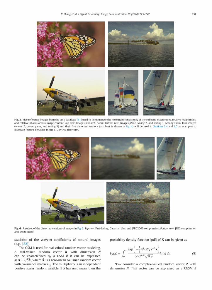
Fig. 3. Five reference images from the LIVE database [81] used to demonstrate the histogram consistency of the subband magnitudes, relative magnitudes,and relative phases across image content. Top row: Images monarch, ocean. Bottom row: Images plane, sailing 2, and sailing 3. Among them, four images(monarch, ocean, plane, and sailing 3) and their five distorted versions (a subset is shown in Fig. 4) will be used in Sections 2.4 and 2.5 as examples toillustrate feature behavior in the C-DIIVINE algorithm.

Fig. 4. A subset of the distorted versions of images in Fig. 3. Top row: Fast-fading, Gaussian blur, and JPEG2000 compression. Bottom row: JPEG compressionand white noise.


statistics of the wavelet coefficients of natural images(e.g., [82]).

The GSM is used for real-valued random vector modeling.A real-valued random vector X with dimension Ncan be characterized by a GSM if it can be expressedas X¼

ffiffiffiS

p~X, where ~X is a zero-mean Gaussian random vector

with covariance matrix C ~X . The multiplier S is an independentpositive scalar random variable. If S has unit mean, then the

probability density function (pdf) of X can be given as

f X xð Þ ¼Z 1

0

exp �12xT ðsC ~X Þ�1x

� �ð2πÞN=2 ffiffiffiffiffiffiffiffi

sC ~X

p f S sð Þ ds: ð8Þ

Now consider a complex-valued random vector Z withdimension N. This vector can be expressed as a CGSM if

0 10 20 30 40 50 60 70 800

0.2

0.4

0.6

0.8

1

Wavelet coefficient magnitude

# of

coe

ffic

ient

s (N

orm

aliz

ed) monarch.bmp

ocean.bmpplane.bmpsailing2.bmpsailing3.bmp

0 5 10 15 200

0.2

0.4

0.6

0.8

1


monarch.bmpocean.bmpplane.bmpsailing2.bmpsailing3.bmp

0 5 10 15 20 25 30 35 400

0.2

0.4

0.6

0.8

1


blurffjp2kjpegrefwn

Fig. 5. Histograms of subband magnitudes for each of the five reference images in Fig. 3 and five distorted versions of image sailing 2 in Fig. 7. Thesemagnitude histograms were generated by using all coefficients from all six subbands at the finest scale, without divisive normalization (a), and withdivisive normalization (b), (c). Notice that the histograms exhibit consistent profiles that are largely independent of the particular reference image fromwhich the magnitudes were computed, but vary significantly in the presence of distortions.

30° orientation 90° orientation 150° orientation

-6 -4 -2 0 2 4 60

0.2

0.4

0.6

0.8

1

Wavelet coefficients relative magnitude

# of

coe

ffic

ient

s (N

orm

aliz

ed)


-6 -4 -2 0 2 4 6 80

0.2

0.4

0.6

0.8

1



-6 -4 -2 0 2 4 6 80

0.2

0.4

0.6

0.8

1



-4 -3 -2 -1 0 1 2 3 40

0.2

0.4

0.6

0.8

1

Wavelet coefficients relative phase

# of

coe

ffic

ient

s (N

orm

aliz

ed)


-4 -3 -2 -1 0 1 2 3 40

0.2

0.4

0.6

0.8

1



-4 -3 -2 -1 0 1 2 3 40

0.2

0.4

0.6

0.8

1



Fig. 6. Histograms of subband relative magnitude (a) and relative phase (b) for each of the five reference images in Fig. 3. These histograms were generatedby using subbands of the indicated orientations at the finest scale. Notice that the histograms exhibit consistent profiles that are largely independent of theparticular reference image from which the relative magnitudes and relative phases were computed. Also notice that the location of the relative phasehistogram peak varies according to the subband's orientation.


Z¼RfZgþ jIfZg ¼ffiffiffiS

p~Z, where ~Z ¼Rf ~Z gþ jIf ~Zg is a zero-

mean complex Gaussian random vector, and where themultiplier S is an independent positive scalar randomvariable.If S has unit mean, then the pdf of Z can be given as

f Z zð Þ ¼Z 1

0

1πN jsC ~Z j

exp �zHðsC ~Z Þ�1z� �

f S sð Þ ds: ð9Þ

where C ~Z ¼ Ef ~Z ~ZHg is the complex covariance matrix. The

vector Z is called a CGSM because of its behavior as a complexGaussian conditioned on S. Here, we see again the significanceof divisive normalization: the definition of CGSM (Z¼

ffiffiffiS

p~Z)

theoretically requires a normalization process (divided byffiffiffiS

p)

to make the output ( ~Z) to be a zero-mean complex Gaussianrandom vector, which can be characterized by the complexgeneralized Gaussian distribution.

2.3.2. Marginal density of magnitudeAs shown by Rakvongthai et al. [75], when N¼1 in

Eq. (9) (i.e., both RfZg and IfZg are characterized by GSMmodel), Z is a complex random variable which can becharacterized by a complex generalized Gaussian distribu-tion. When Z is expressed in radial form as Z ¼ jZjej∠Z , the

Fig. 7. Distorted versions of image sailing 2. From left to right: Fast-fading, Gaussian blur, JPEG2000 compression, JPEG compression, and white noise.

30° orientation 90° orientation 150° orientation

-15 -10 -5 0 5 10 150

0.2

0.4

0.6

0.8

1


# of

coe

ffic

ient

s (N

orm

aliz

ed)

blurffjp2kjpegrefwn

-15 -10 -5 0 5 10 150

0.2

0.4

0.6

0.8

1


blurffjp2kjpegrefwn

-15 -10 -5 0 5 10 150

0.2

0.4

0.6

0.8

1


blurffjp2kjpegrefwn

-4 -3 -2 -1 0 1 2 3 40

0.2

0.4

0.6

0.8

1


# of

coe

ffic

ient

s (N

orm

aliz

ed)

blurffjp2kjpegrefwn

-4 -3 -2 -1 0 1 2 3 40

0.2

0.4

0.6

0.8

1


blurffjp2kjpegrefwn

-4 -3 -2 -1 0 1 2 3 40

0.2

0.4

0.6

0.8

1


blurffjp2kjpegrefwn

Fig. 8. Histograms of subband relative magnitude (a) and relative phase (b) for each of the five distorted versions of image sailing 2 in Fig. 7. The distortionstend to affect the peakedness of the characteristic profile observed for the reference images.


pdf of the magnitude jZj is given by [75]

f jZj jzjð Þ ¼ β

α2Γð2=βÞjzjexp �ðjzj=αÞβ� � ð10Þ

where α¼ sffiffiffiffiffiffiffiffiffiffiffiffiffiffiffiffiffiffiffiffiffiffiffiffiffiffiffiffiffiffiffiffiffi2Γð1=γÞ=Γð2=γÞ

pis a scale parameter, and

where β¼ 2γ is a shape parameter. The parameters s40and γ40 are the parameters of the complex generalizedGaussian distribution from which f jZjðjzjÞ is derived (see[75] for a derivation).

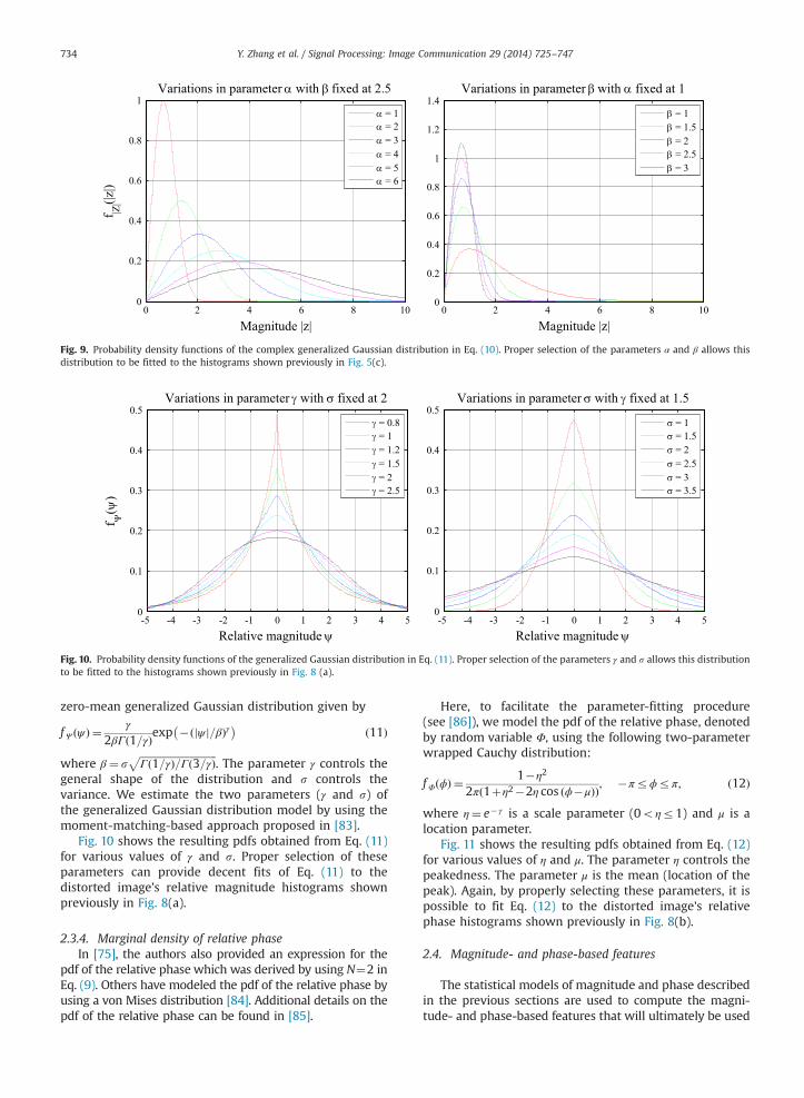
Fig. 9 shows how the parameters α and β affect the pdfsgenerated by Eq. (10). When β is fixed, the parameter α(the scale parameter) controls both the width and thelocation of the peak. When α is fixed, the parameter β

(the shape parameter) controls the rate at which the pdfdecays from its peak. By properly selecting these para-meters, it is possible to provide decent fits of Eq. (10) tothe distorted image's magnitude histograms shown pre-viously in Fig. 5(c).

2.3.3. Marginal density of relative magnitudeDistortions affect not only the coefficient magnitude

distribution as a whole, but also the relationship amongneighboring pixels. Therefore, we also model the marginaldensity of the relative magnitude, which was previouslydefined in Eq. (3). The pdf of the relative magnitude,denoted by random variable Ψ , can be modeled by a

0 2 4 6 8 100

0.2

0.4

0.6

0.8

1Variations in parameter with fixed at 2.5

Magnitude |z|

f |Z|(|z

|) = 1 = 2 = 3 = 4 = 5 = 6

0 2 4 6 8 100

0.2

0.4

0.6

0.8

1

1.2

1.4Variations in parameter with fixed at 1

Magnitude |z|

= 1 = 1.5 = 2 = 2.5 = 3

Fig. 9. Probability density functions of the complex generalized Gaussian distribution in Eq. (10). Proper selection of the parameters α and β allows thisdistribution to be fitted to the histograms shown previously in Fig. 5(c).

-5 -4 -3 -2 -1 0 1 2 3 4 50

0.1

0.2

0.3

0.4

0.5Variations in parameter with fixed at 2

Relative magnitude

f(

)

= 0.8 = 1 = 1.2 = 1.5 = 2 = 2.5

-5 -4 -3 -2 -1 0 1 2 3 4 50

0.1

0.2

0.3

0.4

0.5Variations in parameter with fixed at 1.5

Relative magnitude

= 1 = 1.5 = 2 = 2.5 = 3 = 3.5

Fig. 10. Probability density functions of the generalized Gaussian distribution in Eq. (11). Proper selection of the parameters γ and s allows this distributionto be fitted to the histograms shown previously in Fig. 8 (a).


zero-mean generalized Gaussian distribution given by

f Ψ ψð Þ ¼ γ

2βΓð1=γÞexp �ðjψ j=βÞγ� � ð11Þ

where β¼ sffiffiffiffiffiffiffiffiffiffiffiffiffiffiffiffiffiffiffiffiffiffiffiffiffiffiffiffiffiffiΓð1=γÞ=Γð3=γÞ

p. The parameter γ controls the

general shape of the distribution and s controls thevariance. We estimate the two parameters (γ and s) ofthe generalized Gaussian distribution model by using themoment-matching-based approach proposed in [83].

Fig. 10 shows the resulting pdfs obtained from Eq. (11)for various values of γ and s. Proper selection of theseparameters can provide decent fits of Eq. (11) to thedistorted image's relative magnitude histograms shownpreviously in Fig. 8(a).

2.3.4. Marginal density of relative phaseIn [75], the authors also provided an expression for the

pdf of the relative phase which was derived by using N¼2 inEq. (9). Others have modeled the pdf of the relative phase byusing a von Mises distribution [84]. Additional details on thepdf of the relative phase can be found in [85].

Here, to facilitate the parameter-fitting procedure(see [86]), we model the pdf of the relative phase, denotedby random variable Φ, using the following two-parameterwrapped Cauchy distribution:

f Φ ϕð Þ ¼ 1�η2

2πð1þη2�2η cos ðϕ�μÞÞ; �πrϕrπ; ð12Þ

where η¼ e� γ is a scale parameter (0oηr1) and μ is alocation parameter.

Fig. 11 shows the resulting pdfs obtained from Eq. (12)for various values of η and μ. The parameter η controls thepeakedness. The parameter μ is the mean (location of thepeak). Again, by properly selecting these parameters, it ispossible to fit Eq. (12) to the distorted image's relativephase histograms shown previously in Fig. 8(b).

2.4. Magnitude- and phase-based features

The statistical models of magnitude and phase describedin the previous sections are used to compute the magni-tude- and phase-based features that will ultimately be used

-3 -2 -1 0 1 2 30

0.2

0.4

0.6

0.8

1Variations in parameter with fixed at 0

Relative phase (radians)

f(

) = 0.2 = 0.25 = 0.35 = 0.55 = 0.65 = 0.75 = 0.85

-3 -2 -1 0 1 2 30

0.1

0.2

0.3

0.4

0.5Variations in parameter with fixed at 0.65

Relative phase (radians)

Fig. 11. Probability density functions of the two-parameter wrapped Cauchy distribution in Eq. (12). Proper selection of the parameters η and μ allows thisdistribution to be fitted to the histograms shown previously in Fig. 8 (b).


for quality assessment. As mentioned in Section 1, thesefeatures are computed at multiple scales and orientations tomimic the cortical decomposition in the human visualsystem. Also, note that these magnitude- and phase-basedfeatures are extracted only from the first and second scaleof the wavelet subbands, since most distortion types have apronounced effect on the higher-frequency components,resulting in considerable magnitude and phase distortionsin the high-frequency band. The third scale wavelet sub-bands can indeed represent distortions to some extent.However, due to its relatively smaller coefficient number,such representations can be imprecise compared to theother two scales, and may even decrease the performancewhen employed.

Therefore, given an image decomposed by the complexwavelet transform at three scales and six orientations,resulting in a set of 18 subbands fZs;og, we generate 12vectors containing the coefficient magnitudes, six vectorscontaining the relative magnitudes, 12 vectors containingthe horizontal relative phases, and 12 vectors containingthe vertical relative phases for future analysis. The magni-tude- and phase-based features are then measured asfollows.

2.4.1. Magnitude-based featuresLet jZs;oj and Ψs;o denote the vectors of magnitude and

relative magnitude, respectively, generated by applyingdivisive normalization to and computing the magnitude/relative magnitude of each coefficient in subband Zs;o.Then, we fit the histogram of each vector jZs;oj and Ψs;o

at the finest scale with their corresponding pdfrepresentatives.

Specifically, we fit jZs;oj with Eq. (10) to determine thebest-fitting parameters αs;o and βs;o. For the fitting proce-dure, we employ the maximum-likelihood estimationalgorithm proposed in [87]. We fit Ψs;o with Eq. (11) todetermine the best-fitting parameters γs;o and ss;o. For thefitting procedure, we employ the moment-matching-based approach proposed in [83]. Because there are sixmagnitude and relative magnitude vectors at the finest

scale, we obtain six values of αs;o, βs;o, γs;o, and ss;orespectively, where s¼ 1 and oA ½01;301;601;901;1201;1501�.

We also generate two additional vectors of magnitudes,where each is assembled by grouping all six vectorscorresponding to the same scale into a single vector:

jZsj ¼ ½jZs;01j; jZs;301j; jZs;601j; jZs;901j; jZs;1201j; jZs;1501j�;where sA ½1;2�. In this case, we captured part of theinformation in the lower-frequency bands to fully char-acterize an image. For both vectors (jZ1j and jZ2j), we applythe same histogram-fitting procedure to determine thebest-fitting parameters αs and βs, sA ½1;2�.

Thus, the four resulting magnitude-based feature vec-tors, vα, vβ , vγ , and vs, contain the following 28 elements:

vα ¼ ½α1;01; α1;301;α1;601; α1;901; α1;1201; α1;1501; α1; α2�;vβ ¼ ½β1;01; β1;301; β1;601; β1;901; β1;1201; β1;1501; β1; β2�;vγ ¼ ½γ1;01; γ1;301; γ1;601; γ1;901; γ1;1201; γ1;1501�;vs ¼ ½s1;01; s1;301;s1;601; s1;901; s1;1201; s1;1501�:Following [57], we use the logarithm of the scale para-meter (here lnðαÞ; in [57] lnðs2Þ) rather than the actualscale parameter.

Fig. 12 shows plots of the magnitude-based features forfour reference images (shown in Fig. 3) and their distortedversions (shown in Fig. 4), in which the horizontal axisrepresents the feature index and the vertical axis repre-sents the corresponding feature values. Notice that clus-tering of features across distortions is independent ofimage content.

2.4.2. Phase-based featuresLet Φhorz

s;o and Φverts;o denote vectors of horizontal and

vertical relative phases generated by applying a mappingprocedure to the original relative phases computed byEq. (4) and (5) respectively, of each coefficient in subbandZs;o, where sA ½1;2� and oA ½01;301;601;901;1201;1501�.Then, for each of the vectors Φhorz

s;o and Φverts;o , we fit their

histograms with Eq. (12) to determine the best-fittingparameters ηhorzs;o and ηverts;o . For the fitting procedure, we

0 5 10 15 20 25 30-4

-3

-2

-1

0

1

2

3

4monarch

Mag

nitu

de-b

ased

feat

ures

feature index0 5 10 15 20 25 30

-4

-3

-2

-1

0

1

2

3ocean

Mag

nitu

de-b

ased

feat

ures

feature index

0 5 10 15 20 25 30-4

-3

-2

-1

0

1

2

3sailing3

Mag

nitu

de-b

ased

feat

ures

feature index0 5 10 15 20 25 30

-5

-4

-3

-2

-1

0

1

2

3plane

Mag

nitu

de-b

ased

feat

ures

feature index

Fig. 12. Plots of the magnitude-based features for four reference images and their distorted versions from the LIVE database [81]. For each figure: referenceimage (□), fast fading (▵), blur (○), JPEG2000 (�), JPEG (⋄), and white noise (n).


employ the technique described in [86]. (The parameter μin Eq. (12) is determined largely by the orientation of thesubband and therefore contributes negligibly toward thedistortion identification and quality assessment processes;consequently, we do not store the parameter μ.)

We therefore obtain a single phase-based featurevector, vη, which contains the following 24 elements:

vη ¼ ½ηhorz1;01 ; ηhorz1;301; η

horz1;601; η

horz1;901; η

horz1;1201; η

horz1;1501;

ηhorz2;01 ; ηhorz2;301; η

horz2;601; η

horz2;901; η

horz2;1201; η

horz2;1501;

ηvert1;01; ηvert1;301; η

vert1;601; η

vert1;901; η

vert1;1201; η

vert1;1501;

ηvert2;01; ηvert2;301; η

vert2;601; η

vert2;901; η

vert2;1201; η

vert2;1501�:

Fig. 13 shows plots of the phase-based features for fourreference images (shown in Fig. 3) and their distortedversions (shown in Fig. 4). The axes of each plot havesimilar meanings to those of Fig. 12. For the referenceimages, the values of η tend to be around 0.75. Again,distortion-specific clustering independent of content isobserved.

2.5. Across-scale correlation feature

Another feature employed in DIIVINE, which we alsouse in C-DIIVINE, is a measure of the across-scale

correlations. As argued in [26], degradation of theseacross-scale correlations can lead to marked reductionsin visual quality due to disruptions of the visual system'spreference for integrating edges in a coarse-to-fine-scalefashion.

In the original DIIVINE algorithm, a windowed struc-tural correlation (a component of SSIM [27]) was used tomeasure the across-scale correlations between each sub-band and the high-pass residual (HPR) band obtained fromthe steerable pyramid decomposition. In C-DIIVINE, thewavelet subbands contain complex-valued coefficients,which allow the use of a complex-valued structuralcorrelation measure. Specifically, we employ the complexwavelet structural similarity index (CW-SSIM) [76].

The CW-SSIM index, denoted by ρ, between two bandsZ1 and Z2 is given by

ρ Z1;Z2ð Þ ¼ 2∑Ni ¼ 1jz1ðiÞjjz2ðiÞjþK

∑Ni ¼ 1jz1ðiÞj2þ∑N

i ¼ 1jz2ðiÞj2þK

!

� 2j∑Ni ¼ 1z1ðiÞz2ðiÞnjþK

2∑Ni ¼ 1jz1ðiÞz2ðiÞnjþK

!; ð13Þ

where z1ðiÞ and z2ðiÞ are elements of Z1 and Z2,respectively.

0 5 10 15 20 250.7

0.75

0.8

0.85

0.9

0.95monarch

Phas

e-ba

sed

feat

ures

feature index0 5 10 15 20 25

0.65

0.7

0.75

0.8

0.85

0.9

0.95

1ocean

Phas

e-ba

sed

feat

ures

feature index

0 5 10 15 20 25

0.65

0.7

0.75

0.8

0.85

0.9

0.95

1sailing3

Phas

e-ba

sed

feat

ures

feature index0 5 10 15 20 25

0.65

0.7

0.75

0.8

0.85

0.9

0.95

1plane

Phas

e-ba

sed

feat

ures

feature index

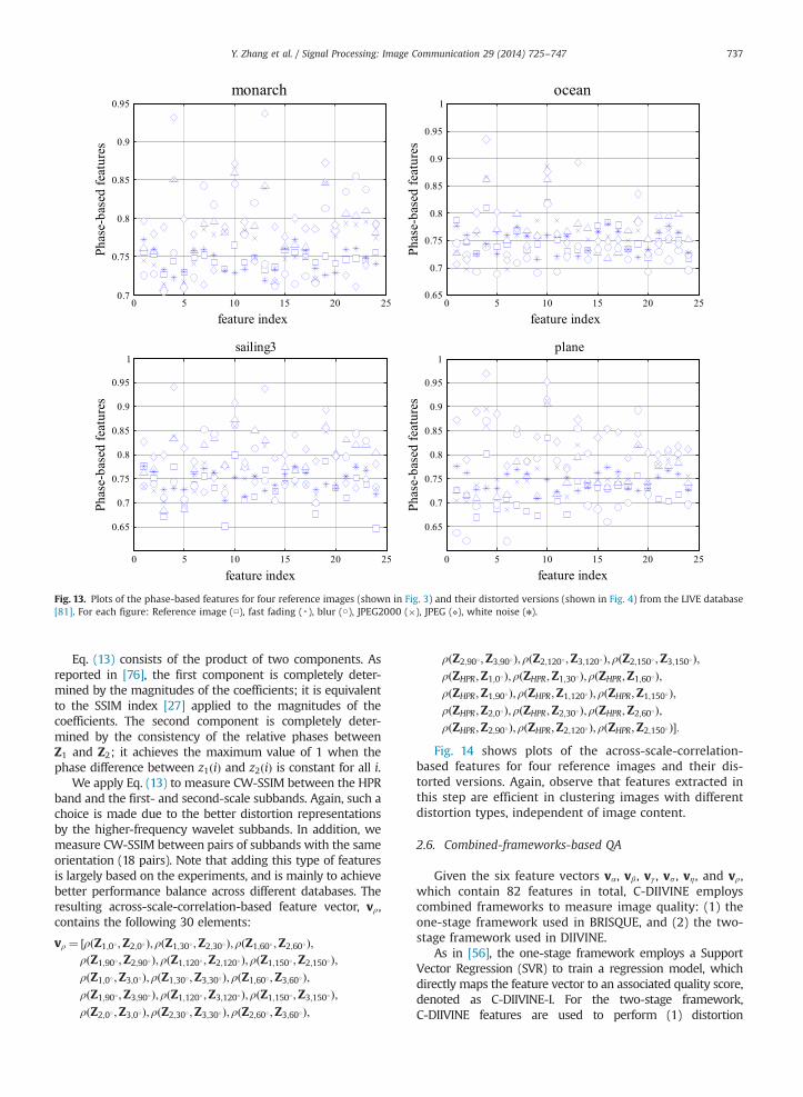
Fig. 13. Plots of the phase-based features for four reference images (shown in Fig. 3) and their distorted versions (shown in Fig. 4) from the LIVE database[81]. For each figure: Reference image (□), fast fading (▵), blur (○), JPEG2000 (�), JPEG (⋄), white noise (n).


Eq. (13) consists of the product of two components. Asreported in [76], the first component is completely deter-mined by the magnitudes of the coefficients; it is equivalentto the SSIM index [27] applied to the magnitudes of thecoefficients. The second component is completely deter-mined by the consistency of the relative phases betweenZ1 and Z2; it achieves the maximum value of 1 when thephase difference between z1ðiÞ and z2ðiÞ is constant for all i.

We apply Eq. (13) to measure CW-SSIM between the HPRband and the first- and second-scale subbands. Again, such achoice is made due to the better distortion representationsby the higher-frequency wavelet subbands. In addition, wemeasure CW-SSIM between pairs of subbands with the sameorientation (18 pairs). Note that adding this type of featuresis largely based on the experiments, and is mainly to achievebetter performance balance across different databases. Theresulting across-scale-correlation-based feature vector, vρ,contains the following 30 elements:

vρ ¼ ½ρðZ1;01;Z2;01Þ; ρðZ1;301;Z2;301Þ; ρðZ1;601;Z2;601Þ;ρðZ1;901;Z2;901Þ; ρðZ1;1201;Z2;1201Þ; ρðZ1;1501;Z2;1501Þ;ρðZ1;01;Z3;01Þ; ρðZ1;301;Z3;301Þ; ρðZ1;601;Z3;601Þ;ρðZ1;901;Z3;901Þ; ρðZ1;1201;Z3;1201Þ; ρðZ1;1501;Z3;1501Þ;ρðZ2;01;Z3;01Þ; ρðZ2;301;Z3;301Þ; ρðZ2;601;Z3;601Þ;

ρðZ2;901;Z3;901Þ; ρðZ2;1201;Z3;1201Þ; ρðZ2;1501;Z3;1501Þ;ρðZHPR;Z1;01Þ; ρðZHPR;Z1;301Þ; ρðZHPR;Z1;601Þ;ρðZHPR;Z1;901Þ; ρðZHPR;Z1;1201Þ; ρðZHPR;Z1;1501Þ;ρðZHPR;Z2;01Þ; ρðZHPR;Z2;301Þ; ρðZHPR;Z2;601Þ;ρðZHPR;Z2;901Þ; ρðZHPR;Z2;1201Þ; ρðZHPR;Z2;1501Þ�:

Fig. 14 shows plots of the across-scale-correlation-based features for four reference images and their dis-torted versions. Again, observe that features extracted inthis step are efficient in clustering images with differentdistortion types, independent of image content.

2.6. Combined-frameworks-based QA

Given the six feature vectors vα, vβ , vγ , vs, vη, and vρ,which contain 82 features in total, C-DIIVINE employscombined frameworks to measure image quality: (1) theone-stage framework used in BRISQUE, and (2) the two-stage framework used in DIIVINE.

As in [56], the one-stage framework employs a SupportVector Regression (SVR) to train a regression model, whichdirectly maps the feature vector to an associated quality score,denoted as C-DIIVINE-I. For the two-stage framework,C-DIIVINE features are used to perform (1) distortion

0 5 10 15 20 25 300

0.05

0.1

0.15

0.2

0.25monarch

Acr

oss-

scal

e co

rrel

atio

n

feature index0 5 10 15 20 25 30

0

0.05

0.1

0.15

0.2

0.25

0.3

0.35ocean

Acr

oss-

scal

e co

rrel

atio

n

feature index

0 5 10 15 20 25 300

0.05

0.1

0.15

0.2

0.25

0.3

0.35sailing3

Acr

oss-

scal

e co

rrel

atio

n

feature index0 5 10 15 20 25 30

0

0.05

0.1

0.15

0.2

0.25

0.3

0.35plane

Acr

oss-

scal

e co

rrel

atio

n

feature index

Fig. 14. Plots of the across-scale-correlation-based features for four reference images (shown in Fig. 3) and their distorted versions (shown in Fig. 4) fromthe LIVE database [81]. For each figure: Reference image (□), fast fading (▵), blur (○), JPEG2000 (�), and JPEG (⋄), white noise (n).


identification, and (2) distortion-specific quality assessment.As in [57], the distortion identification stage employs SupportVector Classification (SVC) to measure the probability that thedistortion in the distorted image falls into one of n distortionclasses, and the distortion-specific quality assessment stageemploys Support Vector Regression (SVR) to obtain n regres-sion modules, each of which maps the feature vectors to anassociated quality score. Note that because each module istrained specifically for each distortion, these regression mod-ules function as distortion-specific quality estimators.

Let p denote the n-dimensional vector of probabilities,and let q denote the n-dimensional vector of estimatedqualities obtained from the n regression modules. Thetwo-stage framework estimated quality, denoted by C-DIIVINE-II, is computed as follows:

C-DIIVINE-II¼ ∑n

i ¼ 1pðiÞqðiÞ; ð14Þ

where p(i) and q(i) denote elements of p and q, respectively.The advantages and disadvantages for both frameworks

are observable. For the two-stage framework, the distortionidentification stage can never be completely correct (due to

the imperfectness of the extracted features and the complex-ity of various distortions), and thus it can always produceidentification errors. The strategy of using a probability-weighted combination rule can help to compensate for theselimitations. However, because of the identification error, itcannot achieve as high a performance as the one-stageframework on the cross-validation test (see Section 3.3). Incomparison, the one-stage framework can help to avoid thispotential error, but test results on the CSIQ and Toyamadatabases (see Section 3.4) show that this framework seemsto be unreliable when the test images possess statisticalproperties not completely observed in the training database.Perhaps this is due to different ranges of feature valuesamong the different databases.

Thus, to take advantages of both frameworks, the finalestimate of quality combines the minimum and averagevalues of the two frameworks' outputs. This approach,denoted by C-DIIVINE, is computed as follows:

C-DIIVINE¼ 12 min C-DIIVINE-I;C-DIIVINE-IIð Þ½þavg C-DIIVINE-I;C-DIIVINE-IIð Þ�¼ 1

2 C-DIIVINE-IþC-DIIVINE-IIð Þ�1

4 jC-DIIVINE-I�C-DIIVINE-IIj: ð15Þ


Eq. (15) is supported by the following observations. First,the minimum operation assumes that the qualities of testimages that were not ‘seen’ in the training database, maybe predicted to have very different qualities. SinceC-DIIVINE was trained on the LIVE database with subjec-tive ratings of degradation expressed in terms of differencemean opinion scores (DMOS) which are positive, thepredicted DMOS value exceed the normal range if thefeature values extracted from a distorted image go beyondthe range of the training database. Thus, the minimumoperation acts to limit the predictions, making them morereliable. Second, the average of the two outputs isemployed as the simplest linearly weighted predictionthat combines the two outputs.

Note that both the SVC and SVR require training, and inour implementation, C-DIIVINE was trained on LIVE usingthe difference mean opinion scores (DMOS) (see Section 3.3).Thus, smaller values of C-DIIVINE denote predictions ofbetter image quality. As we demonstrate next, training thesestages on images from one database can yield excellentpredictive performance on similarly distorted images fromother databases.

3. Results and analysis

In this section, we analyze C-DIIVINE's ability to esti-mate quality. For this task, we evaluate the predictiveperformance of C-DIIVINE on various image quality data-bases. We also compare the performance of C-DIIVINE toother FR and NR IQA algorithms.

3.1. Image-Quality databases

We applied C-DIIVINE to four publicly available data-bases of subjective image quality: (1) the LIVE database[81]; (2) the Toyama database [88]; (3) the TID database[69]; and (4) the CSIQ database [89].

The LIVE database [81], from The University of Texas atAustin, USA, contains 29 original images, between 26 and29 distorted versions of each original image, and subjec-tive ratings of degradation for each distorted image.The database contains five types of distortions: Gaussianblurring (BLUR), additive white noise (WN), JPEG compres-sion, JPEG2000 compression (JP2K), and simulated packet-loss of transmitted JPEG2000-compressed images, whichis also known as fast fading (FF). The subjective ratingswere collected using a double-stimulus scaling paradigm.LIVE contains a total of 779 distorted images and asso-ciated DMOS values.

The Toyama database [88], from the University ofToyama, Japan, contains 14 original images and 12 dis-torted versions of each original, and subjective ratings ofquality for each distorted image (mean opinion scores,MOS values). The database contains two types of distor-tions: JPEG and JPEG2000 compressed images. The sub-jective ratings were collected using a single-stimulusscaling paradigm. Toyama contains a total of 168 distortedimages and associated MOS values.

The TID database [69], from the Tampere Universityof Technology, Finland, contains 25 original images, 68distorted versions of each original image, and subjective

ratings of quality for each distorted image (MOS values).Seventeen types of distortions are present in the database,including JPEG and JPEG2000 compression, and Gaussianblurring (see [69] for a full list). The subjective ratingswere collecting using a double-stimulus scaling paradigm.TID contains a total of 1700 distorted images and asso-ciated MOS values. However, no corresponding standarddeviations are provided with these means, whichprecludes any outlier analysis (see Section 3.2).

The CSIQ database [89], from Oklahoma State Univer-sity, USA, consists of 30 original images, between 24 and30 distorted versions of each original, and subjectiveratings of degradation for each distorted image (DMOSvalues). Six types of distortion are used in CSIQ: JPEGcompression, JPEG2000 compression, global contrastdecrements, additive pink Gaussian noise, additive whiteGaussian noise, and Gaussian blurring. The subjectiveratings were collected using a multiple-stimulus scalingparadigm. CSIQ contains a total of 866 distorted imagesand associated DMOS values.

3.2. Algorithms and performance measures

We compared C-DIIVINE with various FR and NRquality assessment methods for which code is publiclyavailable. The three NR methods compared were BLIINDS-II [90], DIIVINE [57], and BRISQUE [56]), all of whichoperate based on natural-scene statistics and were trainedon LIVE. For the cross-validation test on LIVE, we includedresults of three popular FR IQA algorithms (PSNR [91],SSIM [27], and MS-SSIM [28]) whose results are accessiblein the corresponding papers. We also included C-DIIVINEresults of using only the one-stage and two-stage frame-works denoted by C-DIIVINE-I and C-DIIVINE-II, respec-tively, for comparison. For the cross-database test, two FRIQA algorithms, VIF [29] and MAD [92], were used forcomparison.

Three criteria were used to measure the predictionmonotonicity and prediction accuracy of each algorithm:(1) the Spearman Rank-Order Correlation Coefficient(SROCC), (2) the Pearson Linear Correlation Coefficient(CC), and (3) the Root Mean Square Error (RMSE) afternon-linear regression. As recommended in [93], the SROCCserves as a measure of prediction monotonicity, while theCC and RMSE serve as measures of prediction accuracy.Two additional criteria were used to measure the predic-tion consistency of each algorithm: (1) outlier ratio (OR),and (2) outlier distance (OD) [92].

A QA algorithm might yield predictions of quality thatare nonlinearly related to the actual MOS/DMOS values.Such a nonlinear relationship can lead to a seemingly poorprediction accuracy/consistency when evaluated in termsof CC, RMSE, OR, and OD. As recommended in [93],we accounted for this fact by applying the followingfour-parameter logistic transform to each algorithm'sraw predicted scores before computing the CC, RMSE,OR, and OD:

f xð Þ ¼ τ1�τ2

1þexp �x�τ3jτ4j

� �þτ2; ð16Þ


where x denotes the raw predicted score, and where τ1, τ2, τ3,and τ4 are free parameters selected to provide the best fit ofthe predicted scores to the MOS/DMOS values. Note that theSROCC relies only on the rank-ordering and is thus unaffectedby the logistic transform due to the fact that f(x) is amonotonic function of x that does not change the rank-order.

3.3. Training and cross-validation performance on LIVE

As mentioned in Section 2.6, C-DIIVINE employs com-bined frameworks to predict image quality and eachframework requires training. In this paper, we trainedC-DIIVINE on the LIVE database by using the realignedDMOS values recommended in [94]. The use of the LIVEdatabase for training facilitates a fairer comparison withother FR and NR algorithms; all of these algorithms haveeither been trained on LIVE (for NR IQA) or have beenextensively tested on LIVE (for FR IQA). As in [57], we usedthe libSVM package [95] to implement the training pro-cess. The parameters of the radial basis function kernelused for both the classification and regression were alsooptimized by the training process.

Table 1Median SROCC and CC values across 1000 train-test combinations on theLIVE database. Italicized entries denote NR IQA algorithms; others are FRIQA algorithms.

JP2K JPEG WN BLUR FF ALL

SROCCPSNR 0.8646 0.8831 0.9410 0.7515 0.8736 0.8636SSIM 0.9389 0.9466 0.9635 0.9046 0.9393 0.9129MS-SSIM 0.9627 0.9785 0.9773 0.9542 0.9386 0.9535BLIINDS-II 0.9323 0.9331 0.9463 0.8912 0.8519 0.9124DIIVINE 0.9123 0.9208 0.9818 0.9373 0.8694 0.9250BRISQUE 0.9139 0.9647 0.9786 0.9511 0.8768 0.9395C-DIIVINE-I 0.9343 0.9398 0.9702 0.9275 0.9072 0.9416C-DIIVINE-II 0.9102 0.9434 0.9778 0.9310 0.9021 0.9376C-DIIVINE 0.9302 0.9444 0.9760 0.9386 0.9110 0.9444

CCPSNR 0.8762 0.9029 0.9173 0.7801 0.8795 0.8592SSIM 0.9405 0.9462 0.9824 0.9004 0.9514 0.9065MS-SSIM 0.9746 0.9793 0.9883 0.9645 0.9488 0.9511BLIINDS-II 0.9386 0.9426 0.9635 0.8994 0.8789 0.9164DIIVINE 0.9233 0.9348 0.9866 0.9370 0.8916 0.9270BRISQUE 0.9229 0.9735 0.9851 0.9506 0.9030 0.9424C-DIIVINE-I 0.9471 0.9598 0.9803 0.9329 0.9364 0.9468C-DIIVINE-II 0.9240 0.9553 0.9858 0.9355 0.9237 0.9409C-DIIVINE 0.9429 0.9593 0.9844 0.9412 0.9345 0.9474

Table 2Results of the one-sided t-test performed between SROCC values generated by dstatistically superior, equivalent, or inferior to the algorithm in the column.

PSNR SSIM MS-SSIM BLIINDS-II DIIVIN

PSNR 0 �1 �1 �1 �1SSIM 1 0 �1 1 �1MS-SSIM 1 1 0 1 1BLIINDS-II 1 �1 �1 0 �1DIIVINE 1 1 �1 1 0BRISQUE 1 1 �1 1 1C-DIIVINE-I 1 1 �1 1 1C-DIIVINE-II 1 1 �1 1 1C-DIIVINE 1 1 �1 1 1

We performed two types of training on the LIVEdatabase: (1) training on an 80% subset of the databasefor cross-validation and (2) training on the entire databaseto test performance on other databases (see Sections 3.4.2and 3.4.3). For cross-validation, we randomly selected 80/20% training/testing splits of images from the LIVE data-base and repeated the train-test procedure 1000 times.We compared with three NR and three FR methods interms of median SROCC and CC computed over 1000 trialsand the values are shown in Table 1. In order to evaluatestatistical significance, we also performed a one-sided t-test with a 95% confidence level between SROCC valuesgenerated by these algorithms across the 1000 train-testtrials. The results are shown in Table 2, in which “1”, “0”,“�1” indicate that the mean correlation of the row(algorithm) is statistically superior, equivalent, or inferiorto the mean correlation of the column (algorithm).

To demonstrate that C-DIIVINE features can be used fordifferent distortion identification, Table 3 shows the med-ian and mean classification accuracy of the classifier foreach of the distortions in the LIVE database, as well asacross all distortions. To show the performance consis-tency of each of the algorithms considered here, Fig. 15plots the mean and standard deviation of SROCC valuesacross these 1000 trials for each algorithm.

According to the cross-validation test results, C-DIIVINEperforms statistically the best among all NR IQA algo-rithms considered here. Not only does it improve upon itspredecessor DIIVINE, but also outperforms BLIINDS-II andBRISQUE. Also observed are a slight dip in performance ofC-DIIVINE-I, and even more of a dip for C-DIIVINE-II, ascompared to C-DIIVINE. Such observations demonstratethat (1) the two-stage framework often produce moreprediction errors than does the one-stage framework;and (2) the combined frameworks actually work betterthan using either of the two individual frameworks alone.Compared with FR IQA methods, C-DIIVINE is more con-sistent than PSNR and SSIM, but still remains inferior toMS-SSIM, indicating that there is room for further

ifferent measures. “1”, “0”, “�1” indicates that the algorithm in the row is

E BRISQUE C-DIIVINE-I C-DIIVINE-II C-DIIVINE

�1 �1 �1 �1�1 �1 �1 �11 1 1 1

�1 �1 �1 �1�1 �1 �1 �10 0 1 �10 0 1 �1

�1 �1 0 �11 1 1 0

Table 3Mean and median classification accuracy across 1000 train-test trials.

Classification accuracy (%) JP2K JPEG WN BLUR FF ALL

Median 88.9 91.7 100.0 93.3 73.3 89.4Mean 88.8 90.6 99.5 91.3 72.9 88.7

PSNRSSIM

MS-SSIM

BLIINDS-II

DIIVIN

E

BRISQUE

0.82

0.84

0.86

0.88

0.9

0.92

0.94

0.96

0.98

1

SR

OC

C V

alue

C-DIIV

INE

Fig. 15. Mean SROCC and standard error bars for various algorithmsacross the 1000 train-test trials on the LIVE database.


improvement. In the following sections, we will showmore results of these NR IQA algorithms in assessingimage quality on other databases. We will also furtherdiscuss the roles of the one- and two-stage frameworks inthe IQA task.

3.4. Performance on other databases

In order to demonstrate that the performance ofC-DIIVINE is not bounded by the database on which it istrained, we evaluated the performance of C-DIIVINE onsubsets of the CSIQ, TID, and Toyama databases correspond-ing to the individual distortion types of JPEG, JPEG2000,Gaussian blurring, and additive Gaussian white noise(the distortion types on which C-DIIVINE was trained). Inthis case, we trained C-DIIVINE on the entire set of distortedimages in LIVE, which contains 779 images with five distor-tion types (note that the fast fading distortion type wastrained, but was not tested, because it was not found in CSIQ,TID, and Toyama). Before we evaluate and compare theperformance of C-DIIVINE with other NR IQA approaches,we first investigate on the contributions of each individualfeature type employed in the proposed algorithm.

3.4.1. Contributions of individual statistical featuresTo analyze the contributions of each of the three

feature types (magnitude distribution parameters, phasedistribution parameter, and cross-scale correlations)toward the overall performance, we created six abridgedversions of C-DIIVINE in which each version used only one/two of the three feature types. Specifically, the followingabridged versions were created:

�
Magnitude Distribution Feature only (M); � Phase Distribution Feature only (P); � Scale Correlation only (SC); � Magnitude Distribution FeatureþPhase Distribution
Feature (MþP);

�
Magnitude Distribution FeatureþScale Correlation(MþSC);
�
Phase Distribution FeatureþScale Correlation (PþSC).
Each of these versions was trained on the full LIVEdatabase via the same technique used for trainingC-DIIVINE as described previously in Section 3.3. Thetesting was performed on the aforementioned subsets ofimages from CSIQ, TID, and Toyama. The results of thisanalysis are shown in Table 4 in terms of SROCC and CC.For reference, also shown in Table 4 are the SROCC and CCvalues of the full C-DIIVINE algorithm.

In general, for the CSIQ database, the best performanceis obtained by using all three feature types. For the TIDdatabase, the magnitude and phase distribution featuresseem to be very important, for the overall performance ofusing both feature types (MþP) yields almost equivalentperformance as that use all three of them (MþPþSC).More specifically, the phase-based statistic seems to bemore sensitive to JPEG and blur distortions, whereasthe magnitude-based statistic is more sensitive to theJPEG2000 and Gaussian white noise distortions. For theToyama database, the largest contribution also arises fromthe combination of magnitude and phase.

With regard to the performance when all of the distor-tion types are evaluated together as a set (the row labeled“All” in Table 4), the best performance is achieved whenusing all three feature types. Overall, when looking at theentire database, the phase distribution feature seems tocontribute the most, which also demonstrates the impor-tance of phase information to image quality. Also, theseresults confirm that different distortion types manifest bymodifying different subband statistics. Some distortionsprimarily affect the coefficient magnitudes, some primarilyaffect the coefficient phases and some primarily affect theacross-scale correlation. Thus, all three feature types arerequired to properly estimate quality when all of thedistortion types are evaluated together.

3.4.2. Overall performanceThe overall testing results are shown in Table 5 in terms

of SROCC, CC, RMSE, OR, and OD. Also included areC-DIIVINE-I and C-DIIVINE-II for comparison. Italicizedentries denote NR algorithms. The results of the best-performing FR algorithm in each case are bolded, andresults of the best-performing NR algorithm are italicizedand bolded.

As shown in Table 5, C-DIIVINE performs quite wellon the IQA task as compared with other NR methods.It improves upon DIIVINE and is superior to BLIINDS-II.Further, it even challenges BRISQUE, a spatial domain IQAalgorithm, and some FR IQA methods. Specifically, in termsof prediction monotonicity (SROCC) and prediction accu-racy (CC and RMSE), C-DIIVINE outperforms the otherthree NR IQA algorithms on all databases. In terms ofprediction consistency (OR and OD), C-DIIVINE also per-forms better than DIIVINE and demonstrates across-the-board competitive predictive performance among the fourNR IQA methods.

Table 4SROCC and CC for abridged versions of C-DIIVINE using only one/two of the three feature types. M¼Magnitude Distribution Feature only. SC¼ScaleCorrelation only. P¼Phase Distribution Feature only. MþP¼Magnitude Distribution FeatureþPhase Distribution Feature (no across-scale correlation).MþSC¼Magnitude Distribution FeatureþScale Correlation (no phase). PþSC¼Phase Distribution FeatureþScale Correlation (no magnitude). Forreference, the SROCC and CC values of the full C-DIIVINE algorithm are also included (denoted by MþPþSC).

M P SC MþP PþSC MþSC MþPþSC

CSIQCC

JPEG2000 0.902 0.847 0.889 0.891 0.903 0.905 0.920JPEG 0.934 0.893 0.772 0.947 0.926 0.933 0.961BLUR 0.889 0.761 0.680 0.911 0.799 0.918 0.932WN 0.846 0.639 0.723 0.897 0.788 0.880 0.907All 0.900 0.813 0.783 0.914 0.868 0.914 0.935

SROCCJPEG2000 0.873 0.818 0.859 0.860 0.877 0.882 0.893JPEG 0.894 0.841 0.761 0.899 0.879 0.899 0.916BLUR 0.860 0.782 0.712 0.886 0.823 0.903 0.907WN 0.831 0.627 0.715 0.884 0.780 0.878 0.897All 0.867 0.792 0.769 0.886 0.859 0.897 0.910

TIDCC

JPEG2000 0.904 0.825 0.874 0.923 0.910 0.910 0.936JPEG 0.913 0.931 0.824 0.914 0.932 0.905 0.953BLUR 0.846 0.924 0.865 0.894 0.901 0.894 0.891WN 0.704 0.621 0.584 0.827 0.619 0.813 0.795All 0.730 0.872 0.834 0.921 0.894 0.901 0.925

SROCCJPEG2000 0.900 0.825 0.880 0.919 0.913 0.907 0.937JPEG 0.893 0.900 0.823 0.875 0.902 0.883 0.924BLUR 0.849 0.928 0.877 0.898 0.914 0.899 0.900WN 0.717 0.601 0.578 0.842 0.633 0.825 0.809All 0.792 0.879 0.834 0.919 0.891 0.904 0.921

ToyamaCC

JPEG2000 0.875 0.879 0.751 0.903 0.828 0.785 0.870JPEG 0.905 0.900 0.701 0.869 0.841 0.752 0.884All 0.887 0.889 0.679 0.886 0.830 0.814 0.876

SROCCJPEG2000 0.880 0.876 0.723 0.903 0.797 0.786 0.874JPEG 0.887 0.887 0.698 0.869 0.832 0.828 0.882All 0.883 0.884 0.709 0.885 0.810 0.815 0.877


Compared with C-DIIVINE-I and C-DIIVINE-II, we seethat the proposed combined frameworks achieves a per-formance balance across the different databases. It can beclearly observed that the one-stage framework (C-DII-VINE-I) performs quite well when training on LIVE andtesting on TID. This might be attributed to the considerablesimilarity between the two databases. In fact, the cross-validation test results shown in Section 3.3 also demon-strate that the one-stage framework can be a very goodchoice for decision-making when the training data andtesting data share some common properties, consideringthat the two-stage framework often produces classificationerrors in its identification stage. However, it is alsonoteworthy that C-DIIVINE-I performs slightly worse thanC-DIIVINE-II when testing on CSIQ and Toyama, whichdemonstrates that the two-stage framework is perhapsmore robust. Therefore, combining the two frameworks isa simple, yet effective technique for achieving a reasonablebalance in IQA performance across different databases.

The last rows of the SROCC, CC, and RMSE results inTable 5 show the average SROCC, CC, and RMSE, where the

averages are weighted by the number of distorted imagestested in each database. On an average, C-DIIVINE andBRISQUE demonstrate the best NR QA performance. Notethat OD is dependent on the dynamic range of thedatabase, and therefore cannot be compared across data-bases, only within.

Fig. 16 shows scatter-plots of logistic-transformedC-DIIVINE quality predictions vs. subjective ratings (MOSor DMOS) on different databases. Although for eachdatabase, there are some images whose quality scoresare predicted far from their true MOS/DMOS values, over-all, the proposed C-DIIVINE algorithm can predict qualitywell across the range of MOS/DMOS.

3.4.3. Performance on individual distortion typesIn order to demonstrate that C-DIIVINE can achieve

fairly good quality evaluation across different distortiontypes as long as it has been trained on those distortion types,we also report the performance of C-DIIVINE on subsets of thethree previously mentioned databases corresponding to fourindividual distortion types: JPEG, JPEG2000, Gaussian blurring,

Table 5Overall performances of C-DIIVINE and other algorithms on the Toyama, TID, and CSIQ databases. Italicized entries denote NR algorithms. Results of thebest-performing FR algorithm are bolded, and results of the best-performing NR algorithm are italicized and bolded.

MS-SSIM VIF MAD DIIVINE BLIINDS-II BRISQUE C-DIIVINE-I C-DIIVINE-II C-DIIVINE

CCCSIQ 0.950 0.967 0.974 0.854 0.901 0.924 0.914 0:935 0:935TID 0.912 0.950 0.947 0.877 0.864 0.907 0:931 0.907 0.925Toyama 0.893 0.914 0.941 0.634 0.754 0.850 0.851 0.870 0:876Average 0.929 0.954 0.960 0.830 0.867 0.907 0.910 0.916 0:923

SROCCCSIQ 0.953 0.959 0.967 0.828 0.873 0.900 0.879 0:913 0.910TID 0.897 0.940 0.935 0.891 0.840 0.898 0:922 0.905 0.921Toyama 0.887 0.909 0.936 0.642 0.724 0.848 0.851 0.871 0:877Average 0.924 0.945 0.952 0.822 0.840 0.892 0.889 0.904 0:909

RMSECSIQ 0.089 0.072 0.064 0.147 0.123 0.108 0.115 0:100 0:100TID 0.650 0.495 0.509 0.760 0.798 0.668 0:577 0.668 0.602Toyama 0.564 0.507 0.425 0.968 0.864 0.660 0.656 0.616 0:604Average 0.345 0.277 0.265 0.468 0.456 0.375 0.348 0.365 0:341

ORCSIQ 0.220 0.187 0.157 0.365 0.320 0.262 0.297 0:242 0.247TID 0.734 0.630 0.622 0.706 0.766 0.693 0:641 0.672 0.651Toyama 0.066 0.030 0.024 0.214 0.155 0.066 0.083 0.071 0:065Average 0.369 0.312 0.293 0.457 0.444 0.377 0.380 0:360 0:355

ODCSIQ 6.473 5.013 3.243 24.561 16.318 12.697 14.498 11.810 11:600TID 120.957 78.159 79.194 137.472 162.692 121.259 96:667 113.943 99.832Toyama 3.172 1.397 1.673 16.517 12.685 4:158 5.786 5.380 5.418


and additive Gaussian white noise. The same logistic trans-form was used and the performance for each distortion typewas evaluated based on extracting the corresponding trans-formed scores previously computed when all four distortiontypes were considered. Table 6 shows the results in terms ofSROCC, CC, and RMSE values. Also included are results of threeother NR and FR IQA algorithms for comparison. From thetable, we see that C-DIIVINE provides better predictions onmost distortion types in comparison to BLIINDS-II, DIIVINE,and BRISQUE.When looking at the performance of C-DIIVINE-Iand C-DIIVINE-II, we conclude again that the proposedcombined framework actually takes advantages of both indi-vidual frameworks, and achieves a performance balanceacross different databases on most distortion types.

3.4.4. Performance on reference imagesWe also evaluated the performance of C-DIIVINE on

reference images. For this evaluation, we tested C-DIIVINEon undistorted versions of natural images contained in thethree aforementioned databases (note that only 24 undis-torted natural images in the TID database was tested). Sincethere are no valid human opinion scores for reference imagesin the CSIQ and TID databases, and the true reference imageMOS values contained in the Toyama database are too closeto indicate any useful linear/non-linear relationships, weemployed here a different approach for evaluation. Specifi-cally, we first predicted the original quality score for eachreference image using our algorithm, and then applied thesame logistic transform (the sigmoid function parameterswere estimated by using the distorted images in the samedatabase) defined in Eq. (16) to bring the predicted values onthe same scales as the true MOS/DMOS values for thedistorted images. Finally, for each database, we compared

these linearized estimated DMOS values to the correspondingscatter plots in Fig. 16 to see if they are all located in a regionrepresenting the highest quality. The results are shown inFig. 17.

By referring to both figures (Figs. 16 and 17), we see thatC-DIIVINE works well on most reference images. Specifically,28 out of 30 reference images in the CSIQ database are givenquality scores below 0.2, which indicates that only two ofthem were predicted a bit far away from their true DMOSvalues. Note in Fig. 16 that the reference images in the CSIQdatabase should have DMOS values close to zero. For the TIDdatabase, qualities of all 24 reference images seem to be wellpredicted. It also seems that only one reference image in theToyama database was improperly estimated. Note again inFig. 16 that the undistorted natural images in the TID andToyama databases should have MOS values around/above 5.5and 4.5, respectively. All three results demonstrate that theproposed C-DIIVINE algorithm performs well onmost of thesereference images.

3.5. Computational complexity

Having evaluated the performance of C-DIIVINE and otherNR algorithms on various databases, we now analyze theircomputational complexity. Although C-DIIVINE extends itspredecessor DIIVINE to the complex domain, it is stillcomputationally efficient. To evaluate the computationalcomplexity of each of the three feature types, we measuredthe relative percentage of time required to compute thequality of a 512�512 image. We also compared the overallcomputational complexity of C-DIIVINE with other NR IQAalgorithms (BLIINDS-II, DIIVINE, and BRISQUE) on an imageof resolution 512�640. Note that all of these tests were

Table 6SROCC, CC and RMSE of C-DIIVINE and other quality assessment algorithms on different types of distortion on the CSIQ, TID and Toyama databases.Italicized entries denote NR algorithms. Results of the best-performing FR algorithm are bolded, and results of the best-performing NR algorithm areitalicized and bolded.

MS-SSIM VIF MAD DIIVINE BLIINDS-II BRISQUE C-DIIVINE-I C-DIIVINE-II C-DIIVINE

CCCSIQ

JPEG2000 0.977 0.978 0.983 0.893 0.912 0.896 0.913 0.916 0:920JPEG 0.981 0.988 0.983 0.697 0.912 0.946 0.942 0:966 0.961BLUR 0.959 0.974 0.976 0.898 0.897 0.928 0.912 0.928 0:932WN 0.947 0.961 0.956 0.787 0.897 0:938 0.809 0.921 0.907

TIDJPEG2000 0.975 0.971 0.982 0.896 0.919 0.906 0:947 0.902 0.936JPEG 0.966 0.973 0.961 0.899 0.889 0.950 0:956 0.943 0.953BLUR 0.951 0.942 0.801 0.844 0.825 0.873 0:902 0.872 0.891WN 0.810 0.907 0.819 0:828 0.714 0.810 0.791 0.779 0.795

ToyamaJPEG2000 0.949 0.962 0.961 0.603 0.686 0.869 0.851 0:871 0.870JPEG 0.787 0.900 0.919 0.709 0.826 0.865 0.855 0.873 0:884

SROCCCSIQ

JPEG2000 0.969 0.967 0.975 0.830 0.884 0.867 0.880 0.892 0:893JPEG 0.962 0.970 0.962 0.704 0.881 0.909 0.890 0:921 0.916BLUR 0.972 0.975 0.968 0.871 0.870 0.903 0.881 0:911 0:907WN 0.947 0.957 0.954 0.797 0.886 0:925 0.799 0.911 0.897

TIDJPEG2000 0.973 0.970 0.975 0.907 0.911 0.904 0:947 0.906 0.937JPEG 0.940 0.931 0.925 0.871 0.838 0.911 0.923 0.913 0:924BLUR 0.963 0.958 0.847 0.859 0.826 0.874 0:908 0.887 0.900WN 0.818 0.913 0.833 0:834 0.715 0.823 0.803 0.788 0.809

ToyamaJPEG2000 0.945 0.956 0.955 0.612 0.627 0.867 0.852 0:875 0.874JPEG 0.835 0.907 0.917 0.702 0.820 0.857 0.855 0.865 0:882

RMSECSIQ

JPEG2000 0.067 0.066 0.058 0.130 0.142 0.140 0.129 0.127 0:124JPEG 0.059 0.047 0.057 0.125 0.219 0.099 0.102 0:079 0.084BLUR 0.081 0.065 0.062 0.127 0.126 0.107 0.117 0.107 0:104WN 0.054 0.047 0.050 0.074 0.104 0:058 0.099 0.065 0.071

TIDJPEG2000 0.431 0.459 0.366 1.178 0.756 0.810 0:617 0.827 0.675JPEG 0.435 0.388 0.468 0.741 0.774 0.528 0:497 0.561 0.513BLUR 0.359 0.390 0.694 0.621 0.655 0.566 0:501 0.568 0.527WN 0.359 0.258 0.351 0:343 0.429 0.359 0.375 0.383 0.371

ToyamaJPEG2000 0.398 0.344 0.348 1.007 0.983 0.625 0.662 0:620 0.622JPEG 1.237 0.540 0.488 0.872 0.709 0.622 0.641 0.604 0:579

CSIQ TID Toyama

0

0.2

0.4

0.6

0.8

1

1

DM

OS

Linearized C-DIIVINE

0

1

2

3

4

5

6

7

MO

S


1

2

3

4

5

0 0.25 0.5 0.75 0 2 4 6 1 2 3 4 5

MO

S


CC=0.935 CC=0.925 CC=0.876

Fig. 16. Scatter plots of objective scores predicted by the C-DIIVINE algorithm after logistic transform versus subjective scores on different image databases.Note that the x-axis across all three figures represents the predicted value transformed via Eq. (16); the y-axis represents the true DMOS value for the CSIQdatabase, true MOS value for the TID and Toyama databases.


CSIQ TID Toyama

0 5 10 15 20 25 30 350

0.10.20.30.40.50.60.70.80.9

1

Line

ariz

ed C

-DII

VIN

E

Reference Image Index0 5 10 15 20 25

0

1

2

3

4

5

6

7

8

Line

ariz

ed C

-DII

VIN

E

Reference Image Index1 2 3 4 5 6 7 8 9 10 11 12 13 14

0

1

2

3

4

5

6

7

8

Line

ariz

ed C

-DII

VIN

E

Reference Image Index

Fig. 17. Objective quality scores predicted by the C-DIIVINE algorithm after logistic transform on reference images. Note that the x-axis across all threefigures represents the index of reference images in each database; the y-axis represents the predicted value transformed via Eq. (16).

Table 7Informal complexity analysis of C-DIIVINE. Tabulated values reflect thepercentage of the time devoted to each of the three feature types inC-DIIVINE.

Feature type Percentage of time

Magnitude-based features 51.05Phase-based features 38.03Across-scale correlation features 10.92

Table 8A comparison of the runtime require-ments (seconds) for four NR IQAalgorithms on a 512�640 image.

Algorithm Time (s)

BLIINDS-II 50.67DIIVINE 28.77BRISQUE 0.13C-DIIVINE 12.80


performed by running unoptimized MATLAB code on amodern desktop computer (AMD Phenom II X4 965 Proces-sor at 3.39 GHz, 4.00 GB RAM, Windows 7 Pro 64-bit).The results are shown in Tables 7 and 8, respectively.

As shown in Table 8, C-DIIVINE runs faster than DIIVINEand BLIINDS-II. This is due to the fact that DIIVINEcomputes the spatial correlation statistics of an image,and BLIINDS-II extracts the DCT-based features fromnon-overlapping image blocks, both of which occupy aconsiderable chunk of the processing time. However,C-DIIVINE runs slower than BRISQUE. This is mainlybecause of the divisive normalization, a relatively time-consuming process required for computing the magnitude-based features.

4. Conclusion

We presented an extension of DIIVINE to the complexdomain that, for the first time, incorporates the CGSMmodel to assess image quality without need of a referenceacross a variety of distortion categories. The proposedC-DIIVINE algorithm employs combined frameworks andcomplex statistical features to assess image quality byutilizing both magnitude and phase information of the

wavelet coefficients. Specifically, we use the complexgeneralized Gaussian distribution to model the distribu-tion of wavelet coefficient magnitude, the generalizedGaussian distribution to model the distribution of relativemagnitude, and the wrapped Cauchy distribution to modelthe distribution of relative phase. We also use the CW-SSIM index to capture the correlation between differentimage scales. Results show that C-DIIVINE performs wellon most distorted images from the LIVE, CSIQ, TID andToyama databases, predicting image qualities in a mean-ingful agreement with the subjective human being assess-ment. It achieves higher CC and SROCC compared withDIIVINE and BLIINDS-II on most distortion types from thetesting databases, and even challenges BRISQUE and someof the well-known FR IQA algorithms.

Acknowledgments

This material is based upon work supported by theNational Science Foundation Awards 0917014 and 1054612,and by the U.S. Army Research Laboratory (USARL) and theU.S. Army Research Office (USARO) under contract/grantnumber W911NF-10-1-0015.

References

[1] W. Zeng, S. Daly, S. Lei, Point-wise extended visual masking forJPEG2000 image compression, in: Proceedings on the InternationalConference on Image Processing, vol. 1, 2000, pp. 657–660.

[2] I. Hontsch, L. Karam, Locally adaptive perceptual image coding, IEEETrans. Image Process. 9 (2000) 1472–1483.

[3] C.J. van den Branden Lambrecht, A working spatio-temporal modelof the human visual system for image representation and qualityassessment applications, in: Proceedings of IEEE InternationalConference on Acoustics, Speech, and Signal Processing, 1996,pp. 2291–2294.

[4] S. Winkler, Visual quality assessment using a contrast gain controlmodel, in: IEEE Signal Processing Society Workshop on MultimediaSignal Processing, 1999, pp. 527–532.

[5] T. Lam, L.J. Karam, G.P. Abousleman, Robust image coding usingperceptually-tuned channel- optimized trellis-coded quantization,42nd Midwest Symposium on Circuits and Systems 2 (1999)1131–1134.

[6] J.A. Ferwerda, Fundamentals of spatial vision, Appl. Vis. Percept.Comput. Graphics (1998) 1–27.

[7] B. Walter, S.N. Pattanaik, D.P. Greenberg, Using perceptual texturemasking for efficient image synthesis, Comput. Graph. Forum 21 (3)(2002) 393–399.

http://refhub.elsevier.com/S0923-5965(14)00083-6/sbref2













[8] D.I. Neuhoff, T.N. Pappas, Perceptual coding of images for halftonedisplay, IEEE Trans. Image Process. 3 (4) (1994) 341–354.

[9] Q. Yu, K.J. Parker, Quality issues in blue noise halftoning, in:Proceeding of SPIE Color Imaging: Device Independent Color, ColorHardcopy, and Graphic Arts III: Device, vol. 3300, 1998, pp. 376–385.

[10] S. Lu, H. Pu, C. Lin, A HVS-directed neural-network-based approachfor impulse-noise removal from highly corrupted images, in: Pro-ceedings of the IEEE International Conference on Man and Cyber-netic Systems, vol. 1, 2003, pp. 72–77.

[11] Z. Wang, A.C. Bovik, Mean squared error: love it or leave it? A newlook at signal fidelity measures, IEEE Signal Process. Mag. 26 (1)(2009) 98–117.

[12] B. Moulden, F.A.A. Kingdom, L.F. Gatley, The standard deviation ofluminance as a metric for contrast in random-dot images, Percep-tion 19 (1990) 79–101.

[13] F. Lukas, Z. Budrikis, Picture quality prediction based on a visualmodel, IEEE Trans. Commun. 30 (7) (1982) 1679–1692.

[14] J. Lubin, A visual discrimination model for imaging system designand evaluation, Vis. Models Target Detect. Recognit. (1995) 245–283.

[15] Y. Lai, C.J. Kuo, Image quality measurement using the haar wavelet,Wavelet Appl. Signal Image Process. V Proc. SPIE (1997) 127–138.

[16] S. Daly, The visible differences predictor: an algorithm for theassessment of image fidelity, Digit. Images Hum. Vis. 20 (1993)179–206.

[17] N. Nill, A visual model weighted cosine transform for imagecompression and quality assessment, IEEE Trans. Commun. 33 (6)(1985) 551–557.

[18] P.C. Teo, D.J. Heeger, Perceptual image distortion, Proc. IEEE Conf.Image Process. 2 (1994) 982–986.

[19] S.J.P. Westen, R.L. Lagendijk, J. Biemond, Perceptual image qualitybased on a multiple channel HVS model, in: International Con-ference on Acoustics, Speech, and Signal Processing, vol. 4, 1995,pp. 2351–2354.

[20] A.B. Watson, M. Taylor, R. Borthwick, Image quality and entropymasking, Hum. Vis. Electron. Imaging II Proc. SPIE 3016 (1997)2–12.

[21] S. Winkler, A perceptual distortion metric for digital color images,in: Proceedings of IEEE International Conference on Image Proces-sing, vol. 3, 1998, pp. 399–403.

[22] A. Bradley, A wavelet visible difference predictor, IEEE Trans. ImageProcess. 8 (1999) 717–730.

[23] P. LeCallet, A. Saadane, D. Barba, Frequency and spatial pooling ofvisual differences for still image quality assessment, Proc. SPIE Hum.Vis. Electr. Imaging V 3959 (2000) 595–603.

[24] N. Damera-Venkata, T.D. Kite, W. Geisler, B.L. Evans, A.C. Bovik,Image quality assessment based on a degradation model, IEEE Trans.Image Process. 9 (2000) 636–650.

[25] M. Carnec, P.L. Callet, D. Barba, An image quality assessment methodbased on perception of structural information, in: Proceedings ofInternational Conference on Image Processing, vol. 3, 2003, pp. 185–188.

[26] D.M. Chandler, S.S. Hemami, VSNR: a wavelet-based visual signal-to-noise ratio for natural images, IEEE Trans. Image Process. 16 (9)(2007) 2284–2298.

[27] Z. Wang, A.C. Bovik, H.R. Sheikh, E.P. Simoncelli, Image qualityassessment: from error visibility to structural similarity, IEEE Trans.Image Process. 13 (4) (2004) 600–612.

[28] Z. Wang, E.P. Simoncelli, A.C. Bovik, Multiscale structural similarityfor image quality assessment, in: Conference Record of the Thirty-Seventh Asilomar Conference on Signals, Systems and Computers,vol. 2, 2003, pp. 1398–1402.

[29] H.R. Sheikh, A.C. Bovik, Image information and visual quality, IEEETrans. Image Process. 15 (2) (2006) 430–444.

[30] G. Zhai, W. Zhang, X. Yang, Image quality assessment metrics basedon multi-scale edge presentation, in: IEEE Workshop Signal Proces-sing Systems Design and Implementation, 2005, pp. 331–336.

[31] C.-L. Yang, W.-R. Gao, L.-M. Po, Discrete wavelet transform-basedstructural similarity for image quality assessment, in: 15th IEEEInternational Conference on Image Processing, 2008, pp. 377–380.

[32] M. Zhang, X. Mou, A psychovisual image quality metric based onmulti-scale structure similarity, in: IEEE International Conference onImage Processing, 2008, pp. 381–384.

[33] A. Shnayderman, A. Gusev, A.M. Eskicioglu, An SVD-based grayscaleimage quality measure for local and global assessment, IEEE Trans.Image Process. 15 (2) (2006) 422–429.

[34] Z. Wang, E.P. Simoncelli, Reduced-reference image quality assess-ment using a wavelet-domain natural image statistic model, Proc.SPIE Hum. Vis. Electron. Imaging X 5666 (2005).

[35] K. Chono, Y.-C. Lin, D.P. Varodayan, Y. Miyamoto, B. Girod, Reduced-reference image quality assessment using distributed source coding,

in: IEEE International Conference on Multimedia and Expo, 2008,pp. 609–612.

[36] W. Xue, X. Mou, Reduced-reference image quality assessment basedon weibull statistics, in: International Workshop on Quality ofMultimedia Experience, 2010, pp. 1–6.

[37] Z. Wang, H.R. Sheikh, A.C. Bovik, No-reference perceptual qualityassessment of JPEG compressed images, in: Proceedings of IEEEInternational Conference on Image Processing, vol. 1, 2002, pp. 477–480.

[38] L. Meesters, J.B. Martens, A single-ended blockiness measure forJPEG-coded images, Signal Process. 82 (3) (2002) 369–387.

[39] Y. Horita, S. Arata, T. Murai, No-reference image quality assessmentfor JPEG/JPEG2000 coding, in: European Signal Processing Confer-ence, 2004, pp. I301–I304.

[40] H. Tong, M. Li, H. Zhang, C. Zhang, No-reference quality assessmentfor JPEG2000 compressed images, in: International Conference onImage Processing, vol. 5, 2004, pp. 3539–3542.

[41] M.G. Choi, J.H. Jung, J.W. Jeon, No-reference image quality assess-ment using blur and noise, World Acad. Sci. Eng. Technol. (2009)163–167.

[42] C. Mingjun, A.C. Bovik, No-reference image blur assessment usingmultiscale gradient, in: International Workshop on Quality of Multi-media Experience, 2009, pp. 70–74.

[43] Y.-C. Chung, J.-M. Wang, R.R. Bailey, S.-W. Chen, S.-L. Chang, A non-parametic blur measure based on edge analysis for image processingapplications, in: Proceedings of IEEE Conference on Cybernetics andIntelligent Systems, vol. 1, 2004, pp. 356–360.

[44] Y.-C. Chung, S.-L. Chang, J.-M. Wang, S.-W. Chen, An edge analysisbased blur measure for image processing applications, J. TaiwanNormal Univ. Math. Sci. Technol. 51 (1) (2006) 21–31.

[45] L. Liang, J. Chen, S. Ma, D. Zhao, W. Gao, A no-reference perceptualblur metric using histogram of gradient profile sharpness, in: 16thIEEE Conference on Image Processing, 2009, pp. 4369–4372.

[46] C.T. Vu, D.M. Chandler, S3: A spectral and spatial sharpness measureof local perceived sharpness in natural images, IEEE Trans. ImageProcess. 21 (3) (2012) 934–945.

[47] D. Shaked, I. Tastl, Sharpness measure: towards automatic imageenhancement, in: IEEE Conference on Image Processing, vol. 1, 2005,pp. 937–940.

[48] A. Ciancio, A.L.N.T. da Costa, E.A.B. da Silva, A. Said, R. Samadani,P. Obrador, No-reference blur assessment of digital pictures based onmultifeature classifiers, IEEE Trans. Image Process. 20 (1) (2011) 64–75.

[49] P. Ye, D. Doermann, No-reference image quality assessment basedon visual codebook, in: 18th IEEE International Conference on ImageProcessing, 2011, pp. 3089–3092.

[50] P. Ye, D. Doermann, No-reference image quality assessment using visualcodebook, IEEE Trans. Image Process. 21 (7) (2012) 3129–3138.

[51] D.J. Field, Relations between the statistics of natural images and theresponse properties of cortical cells, J. Opt. Soc. Am. A 4 (1987)2379–2394.

[52] B.A. Olshausen, D.J. Field, Sparse coding with an overcomplete basisset: a strategy employed by V1? Vis. Res. 37 (1996) 3311–3325.

[53] E.P. Simoncelli, B.A. Olshausen, Natural image statistics and neuralrepresentation, Annu. Rev. Neurosci. 24 (2001) 1193–1216.

[54] S. Gabarda, G. Cristobal, Blind image quality assessment throughanisotropy, J. Opt. Soc. Am. A 24 (2007) B42–B51.

[55] M.A. Saad, A.C. Bovik, C. Charrier, A DCT statistics-based blind imagequality index, IEEE Signal Process. Lett. 17 (2010) 583–586.

[56] A. Mittal, A.K. Moorthy, A.C. Bovik, No-reference image qualityassessment in the spatial domain, IEEE Trans. Image Process. 21(12) (2012) 4695–4708.

[57] A.K. Moorthy, A.C. Bovik, Blind image quality assessment: fromnatural scene statistics to perceptual quality, IEEE Trans. ImageProcess. 20 (12) (2011) 3350–3364.

[58] E.P. Simoncelli, W.T. Freeman, The steerable pyramid: a flexiblearchitecture for multi-scale derivative computation, in: Proceedingsof International Conference on Image Processing, vol. 3, 1995,pp. 444–447.

[59] D.J. Field, Scale-invariance and self-similar ‘wavelet’ transforms: ananalysis of natural scenes and mammalian visual systems, in:Wavelets, Fractals and Fourier Transforms: New Development andNew Applications, 1993, pp. 151–193.

[60] D.J. Field, What is the goal of sensory coding? Neural Comput. 6(1994) 559–601.

[61] W.E. Vinje, J.L. Gallant, Sparse coding and decorrelation in primaryvisual cortex during natural vision, Science 287 (5456) (2000)1273–1276.

[62] D.J. Tolhurst, Y. Tadmor, T. Chao, Amplitude spectra of naturalimages, Ophthal. Phys. Opt. 12 (2) (1992) 229–232.

























































































[63] A.V. Oppenheim, J.S. Lim, The importance of phase in signals, Proc.IEEE 69 (1981) 529–541.

[64] M.G.A. Thomson, D.H. Foster, R.J. Summers, Human sensitivity tophase perturbations in natural images: a statistical framework,Perception 29 (2000) 1057–1069.

[65] P.J. Bex, W. Makous, Spatial frequency, phase, and the contrast ofnatural images, J. Opt. Soc. Am. A 19 (2002) 1096–1106.

[66] W.S. Geisler, J.S. Perry, B.J. Super, D.P. Gallogly, Edge co-occurrencein natural images predicts contour grouping performance, Vis. Res.41 (2001) 711–724.

[67] M.J. Morgan, J. Ross, A. Hayes, The relative importance of local phaseand local amplitude in patchwise image reconstruction, Biol.Cybern. 65 (2) (1991) 113–119.

[68] D.J. Field, D.M. Chandler, Method for estimating the relative con-tribution of phase and power spectra to the total information innatural-scene patches, J. Opt. Soc. Am. A 29 (1) (2012) 55–67.

[69] N. Ponomarenko, V. Lukin, A. Zelensky, K. Egiazarian, M. Carli,F. Battisti, TID2008 – a database for evaluation of full-referencevisual quality assessment metrics, Adv. Mod. Radioelectron. 10(2009) 30–45.

[70] J.G. Daugman, Two-dimensional spectral analysis of cortical recep-tive field profiles, Vis. Res. 20 (10) (1980) 847–856.

[71] J.G. Daugman, Uncertainty relation for resolution in space, andorientation optimized by two-dimensional visual cortical filters, J.Opt. Soc. Am. 2 (27) (1985) 1160–1169.

[72] S. Marcelja, Mathematical description of the response of simplecortical cells, J. Opt. Soc. Am. 70 (11) (1980) 1297–1300.

[73] J.P. Jones, L.A. Palmer, An evaluation of the two-dimensional Gaborfilter model of simple receptive fields in cat striate cortex, J.Neurophysiol. 58 (6) (1987) 1233–1258.

[74] G. Wallis, Linear models of simple cells: correspondence to real cellresponses and space spanning properties, Spat. Vis. 14 (3–4) (2001)237–260.

[75] Y. Rakvongthai, A.P.N. Vo, S. Oraintara, Complex Gaussian scalemixtures of complex wavelet coefficients, IEEE Trans. Signal Process.58 (7) (2010) 3545–3556.

[76] Z. Wang, E.P. Simoncelli, Translation insensitive image similarity inthe complex wavelet domain, in: Proceedings of IEEE InternationalConference on Acoustics Speech and Signal Processing, 2005,pp. 573–576.

[77] A.B. Watson, J.A. Solomon, A model of visual contrast gain controland pattern masking, J. Opt. Soc. Am. A 14 (1997) 2378–2390.

[78] D.J. Heeger, Normalization of cell responses in cat striate cortex, Vis.Neurosci. 9 (1992) 181–197.

[79] M.J. Wainwright, O. Schwartz, E.P. Simoncelli, Natural image statis-tics and divisive normalization: modeling nonlinearity and adapta-tion in cortical neurons, In: Probabilistic Models of the Brain:Perception and Neural Function, 2002, pp. 203–222.

[80] Q. Li, Z. Wang, Reduced-reference image quality assessment usingdivisive normalization-based image representation, IEEE J. Sel.Topics Signal Process. 3 (2) (2009) 202–211.

[81] H.R. Sheikh, Z. Wang, A.C. Bovik, L. K. Cormack, Image and videoquality assessment research at LIVE, ⟨http://live.ece.utexas.edu/research/quality/⟩.

[82] M.J. Wainwright, E.P. Simoncelli, Scale mixture of Gaussians and thestatistics of natural images, Adv. Neural Inf. Process. Syst. 12 (2000)855–861.

[83] K. Sharifi, A. Leon-Garcia, Estimation of shape parameter for gen-eralized Gaussian distribution in subband decompositions of video,IEEE Trans. Circuits Syst. Video Technol. 5 (1) (1995) 52–56.

[84] S.O.A. Vo, T. Nguyen, Using phase and magnitude information of thecomplex directional filter bank for texture image retrieval, in:Proceedings of International Conference on Image Processing, vol.4, 2007, pp. IV–61–IV–64.

[85] A. Vo, S. Oriaintara, N. Nguyen, Vonn distribution of relative phasefor statistical image modeling in complex wavelet domain, SignalProcess. 91 (1) (2011) 114–125.

[86] A. Vo, S. Oraintara, A study of relative phase in complex waveletdomain: property, statistics and applications in texture imageretrieval and segmentation, Signal Process. Image Commun. 25 (1)(2010) 28–46.

[87] Y. Rakvongthai, S. Oriaintara, Statistical image modeling with themagnitude probability density function of complex wavelet coeffi-cients, in: IEEE International Symposium on Circuits and Systems,2009, pp. 1879–1882.

[88] Y. Horita, K. Shibata, Y. Kawayoke, Z.M.P. Sazzad, Subjective qualityassessment Toyama database, ⟨http://mict.eng.u-toyama.ac.jp/mictdb.html⟩.

[89] See ⟨http://vision.okstate.edu/csiq/⟩.[90] M.A. Saad, A.C. Bovik, Blind image quality assessment: a natural

scene statistics approach in the DCT domain, IEEE Trans. ImageProcess. 21 (2012) 3339–3352.

[91] A. T1.TR.74-2001, Objective Video Quality Measurement Using aPeak-Signal-to-Noise-Ratio (PSNR) Full Reference Technique (2001).

[92] E.C. Larson, D.M. Chandler, Most apparent distortion: full-referenceimage quality assessment and the role of strategy, J. Electron.Imaging 19 (1) (2010) 011006.

[93] VQEG, Final Report from the Video Quality Experts Group on theValidation of Objective Models of Video Quality Assessment, PhaseII, ⟨http://www.its.bldrdoc.gov/vqeg/projects/frtv-phase-ii/frtv-phase-ii.aspx⟩(2003).

[94] H.R. Sheikh, M.F. Sabir, A.C. Bovik, A statistical evaluation of recentfull reference image quality assessment algorithms, IEEE Trans.Image Process. 15 (11) (2006) 3440–3451.

[95] C.-C. Chang, C.-J. Lin, LIBSVM: a library for support vector machines,ACM Trans. Intell. Syst. Technol. 2 (3) (2011) 27:1–27:27.












































http://live.ece.utexas.edu/research/quality/

http://live.ece.utexas.edu/research/quality/










http://mict.eng.u-toyama.ac.jp/mictdb.html

http://mict.eng.u-toyama.ac.jp/mictdb.html

http://vision.okstate.edu/csiq/







http://www.its.bldrdoc.gov/vqeg/projects/frtv-phase-ii/frtv-phase-ii.aspx

http://www.its.bldrdoc.gov/vqeg/projects/frtv-phase-ii/frtv-phase-ii.aspx






Documents

Signal Processing: Image Communication - …vision.eng.shizuoka.ac.jp/pubs/pdfs/Yi_SPIC_2014.pdf726 Y. Zhang et al. / Signal Processing: Image Communication 29 (2014) 725–747 type