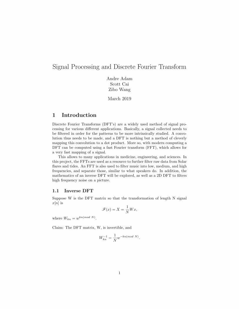
Signal Processing and Discrete Fourier Transform

Andre AdamScott CaiZibo Wang

March 2019

1 Introduction

Discrete Fourier Transforms (DFT’s) are a widely used method of signal pro-cessing for various different applications. Basically, a signal collected needs tobe filtered in order for the patterns to be more intrinsically studied. A convo-lution thus needs to be made, and a DFT is nothing but a method of cleverlymapping this convolution to a dot product. More so, with modern computing aDFT can be computed using a fast Fourier transform (FFT), which allows fora very fast mapping of a signal.

This allows to many applications in medicine, engineering, and sciences. Inthis project, the FFTs are used as a resource to further filter raw data from Solarflares and tides. An FFT is also used to filter music into low, medium, and highfrequencies, and separate those, similar to what speakers do. In addition, themathematics of an inverse DFT will be explored, as well as a 2D DFT to filtershigh frequency noise on a picture.

1.1 Inverse DFT

Suppose W is the DFT matrix so that the transformation of length N signalx[n] is

F (x) = X =1

NWx,

where Wkn = wkn(mod N).

Claim: The DFT matrix, W, is invertible, and

W−1kn =

1

Nw−kn(mod N).

1

Proof: The DFT matrix can be treated as a Vandermonde matrix, i.e.:

W =

(w0)0 (w0)1 (w0)2 (w0)3 ... (w0)N

(w1)0 (w1)1 (w1)2 (w1)3 ... (w1)N

(w2)0 (w2)1 (w2)2 (w2)3 ... (w2)N

...

,which has determinant

det(W ) =∏

0<i<j<N

(wi − wj).

Since all wi are distinct, i.e. wi − wj 6= 0 as long as i 6= j, the determinant ofW thus is non-zero, and so it is invertible.

To verify its inverse has the form stated above:

x[n]?=

1

N

N−1∑k=0

X[k]wkn(mod N)

=1

N

N−1∑k=0

(N−1∑l=0

x[l]wkl(mod N)

)wkn(mod N)

=1

N

N−1∑k=0

N−1∑l=0

x[l]wk(l−n)(mod N)

=1

N

N−1∑k=0

N−1∑l=0

x[l]δ((l − n)(mod N))

=1

N

N−1∑k=0

x[n]

=1

NNx[n] = x[n]

�

1.2 Zero padding

A circular convolution of two signals, x and y, can be computed using FFT andIFFT:

ifft(fft(x).*fft(y))

If two signals are aperiodic with arbitrary length, padding them with zeros allowus to calculate their convolution. Suppose

x = [1, 3,−1, 3], y = [2,−1, 4].

2

First pad each signal with enough zeros to make the common length N =Nx +Ny − 1, which in this case would be 6:

x = [1, 3,−1, 3, 0, 0], y = [2,−1, 4, 0, 0, 0].

Then the convolution can be calculated by hand:

x ∗ y = ( 1, 3,−1, 3, 0, 0)× 2

+ ( 0, 1, 3,−1, 3, 0)× (−1)

+ ( 0, 0, 1, 3,−1, 3)× 4

+ ( 3, 0, 0, 1, 3,−1)× 0

+ (−1, 3, 0, 0, 1, 3)× 0

= ( 2, 5,−1, 19,−7, 12)

The command

ifft(fft([1 3 -1 3 0 0]).*fft([2 -1 4 0 0 0]))

returns the same result.However, if not enough padding zeros, the result would not be a convolution.

Suppose now the padded signals are:

x = [1, 3,−1, 3], y = [2,−1, 4, 0].

the result becomes:

( 1, 3,−1, 3)× 2

+( 3, 1, 3,−1)× (−1)

+(−1, 3, 1, 3)× 4

+( 3,−1, 3, 1)× 0

=(−5, 17,−1, 19)

Again, the same result can be get using command:

ifft(fft([1 3 -1 3]).*fft([2 -1 4 0])).

The reason, from the point of view of how we preform the convolution byhand, it the common length or the period of signal is wrong. From the point ofview of using FFT and IFFT is that, the FFT turn the signal from time domainto frequency domain, with same sample number, i.e. in discrete case, lengthof vector is same in both domain. When not enough zeros are padded, theresolution in frequency domain is too low so that it cannot represent the wholepicture of the signal; therefore, after performing the dot product in frequencydomain, and then turning the result of dot product back into time domain usingIFFT, what comes out is a distorted convolution.

3

2 Audio filter

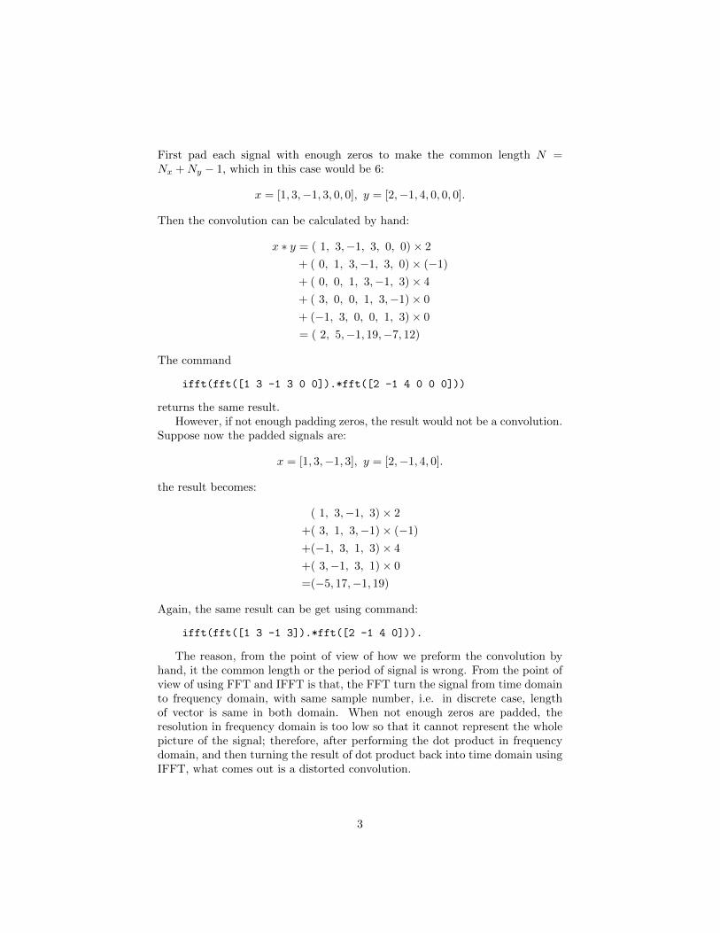
We can use FFT help us filter signals. Since filter noise with certain frequencyin time domain in practical can be hard to conduct, we can use FFT to turnthe signals to frequency domain, eliminate certain frequency, and then inverseFFT to give filtered signals. For example here is an audio clip:

(a) Time domain plot (b) Frequency domain plot

Figure 1: An audio clip

Notice, because of the nature of the Fourier transform, in frequency domainplot, low frequency is at two ends, and high frequency is at the center. From thefrequency domain plot, the dominant frequency is less than about 1/15 highestfrequency. Therefore, a reasonable low, medium, and high frequency rangeswould be 0 < flow < 1/30fmax, 1/30fmax < fmedium < 2/30fmax, 2/30fmax <fhigh.

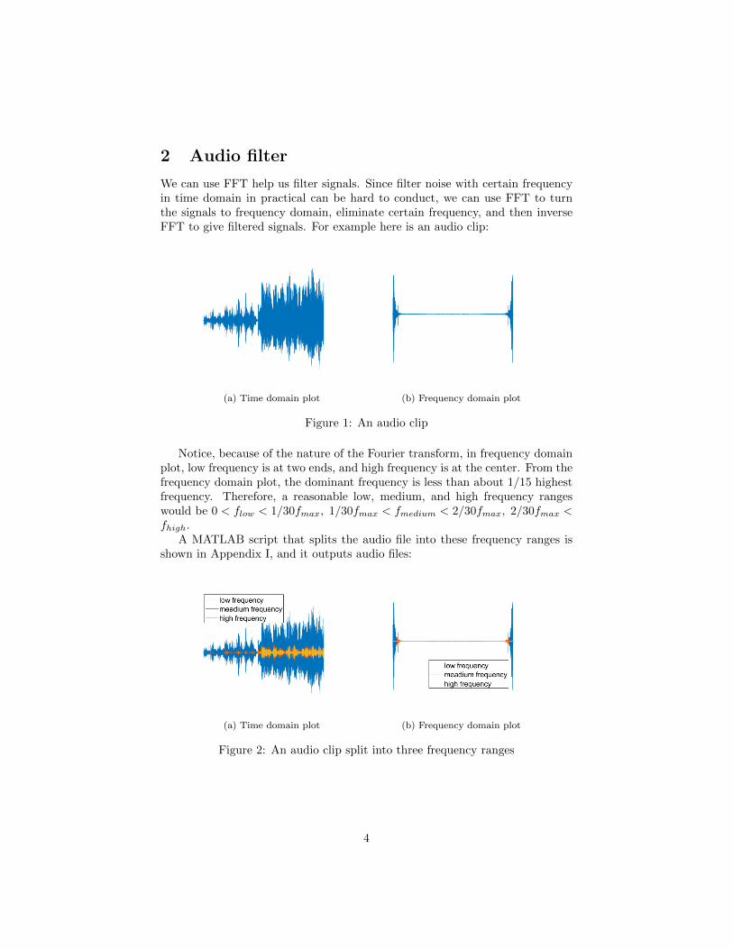
A MATLAB script that splits the audio file into these frequency ranges isshown in Appendix I, and it outputs audio files:

(a) Time domain plot (b) Frequency domain plot

Figure 2: An audio clip split into three frequency ranges

4

3 Tidal Frequency

Historically, FFT’s and DFT’s were first used by Lord Kelvin to analyze andpredict tides in the ocean. With much more computing power nowadays, suchan analysis can be easily made using MatLab’s function for FFT.

Tides are well studied and documented phenomena, with years worth of dataavailable at some of the major scientific databases. In particular, the NationalOceanic and Atmospheric Administration (NOAA for short) has data on tidesavailable since the year of 1964, and closely tracks changes. Predictions are madeevery 6 minutes, and although the verification schedule may change dependingon the location, it is done at least 2 times a day.

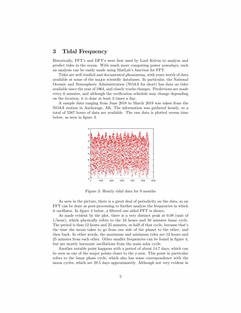
A sample data ranging from June 2018 to March 2019 was taken from theNOAA station in Anchorage, AK. The information was gathered hourly, so atotal of 5567 hours of data are available. The raw data is plotted versus timebelow, as seen in figure 3.

Figure 3: Hourly tidal data for 9 months

As seen in the picture, there is a great deal of periodicity on the data, so anFFT can be done as post-processing to further analyze the frequencies in whichit oscillates. In figure 4 below, a filtered one sided FFT is shown.

As made evident by the plot, there is a very distinct peak at 0.08 (unit of1/hour), which physically refers to the 24 hours and 50 minutes lunar cycle.The period is thus 12 hours and 25 minutes, or half of that cycle, because that’sthe time the moon takes to go from one side of the planet to the other, andthen back. In other words, the maximum and minimum tides are 12 hours and25 minutes from each other. Other smaller frequencies can be found in figure 4,but are mostly harmonic oscillations from the main solar cycle.

Another notable point happens with a period of about 14.7 days, which canbe seen as one of the major points closer to the y-axis. This point in particularrefers to the lunar phase cycle, which also has some correspondence with themoon cycles, which are 29.5 days approximately. Although not very evident in

5

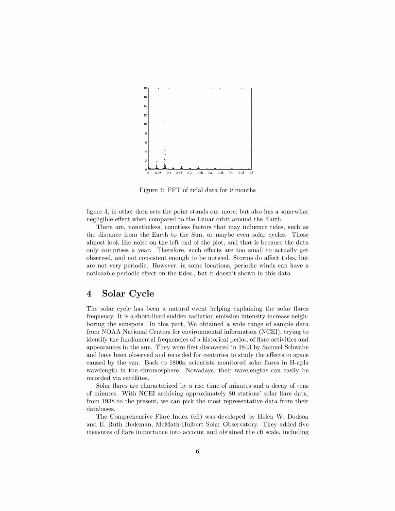
Figure 4: FFT of tidal data for 9 months

figure 4, in other data sets the point stands out more, but also has a somewhatnegligible effect when compared to the Lunar orbit around the Earth.

There are, nonetheless, countless factors that may influence tides, such asthe distance from the Earth to the Sun, or maybe even solar cycles. Thosealmost look like noise on the left end of the plot, and that is because the dataonly comprises a year. Therefore, such effects are too small to actually getobserved, and not consistent enough to be noticed. Storms do affect tides, butare not very periodic. However, in some locations, periodic winds can have anoticeable periodic effect on the tides., but it doesn’t shown in this data.

4 Solar Cycle

The solar cycle has been a natural event helping explaining the solar flaresfrequency. It is a short-lived sudden radiation emission intensity increase neigh-boring the sunspots. In this part, We obtained a wide range of sample datafrom NOAA National Centers for environmental information (NCEI), trying toidentify the fundamental frequencies of a historical period of flare activities andappearances in the sun. They were first discovered in 1843 by Samuel Schwabeand have been observed and recorded for centuries to study the effects in spacecaused by the sun. Back to 1800s, scientists monitored solar flares in H-aplawavelength in the chromosphere. Nowadays, their wavelengths can easily berecorded via satellites.

Solar flares are characterized by a rise time of minutes and a decay of tensof minutes. With NCEI archiving approximately 80 stations’ solar flare data,from 1938 to the present, we can pick the most representative data from theirdatabases.

The Comprehensive Flare Index (cfi) was developed by Helen W. Dodsonand E. Ruth Hedeman, McMath-Hulbert Solar Observatory. They added fivemeasures of flare importance into account and obtained the cfi scale, including

6

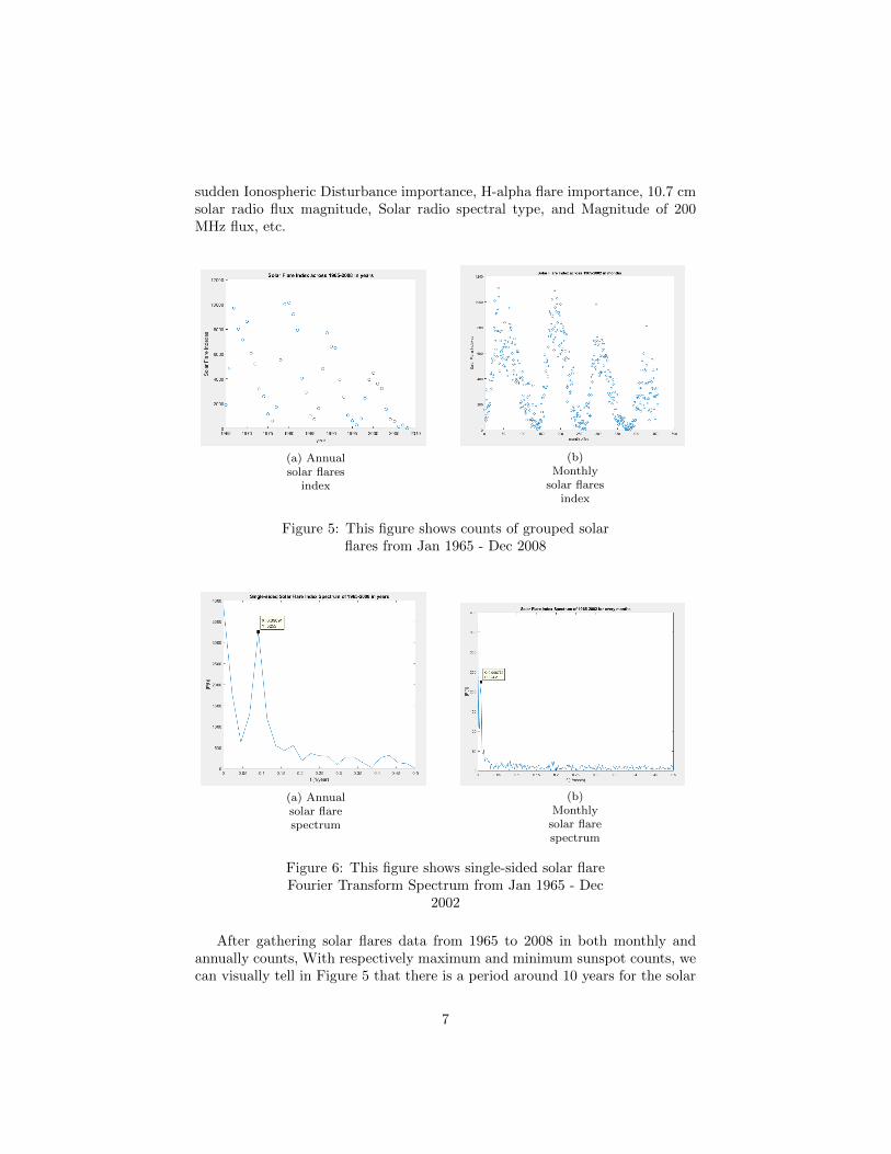
sudden Ionospheric Disturbance importance, H-alpha flare importance, 10.7 cmsolar radio flux magnitude, Solar radio spectral type, and Magnitude of 200MHz flux, etc.

(a) Annualsolar flares

index

(b)Monthly

solar flaresindex

Figure 5: This figure shows counts of grouped solarflares from Jan 1965 - Dec 2008

(a) Annualsolar flarespectrum

(b)Monthly

solar flarespectrum

Figure 6: This figure shows single-sided solar flareFourier Transform Spectrum from Jan 1965 - Dec

2002

After gathering solar flares data from 1965 to 2008 in both monthly andannually counts, With respectively maximum and minimum sunspot counts, wecan visually tell in Figure 5 that there is a period around 10 years for the solar

7

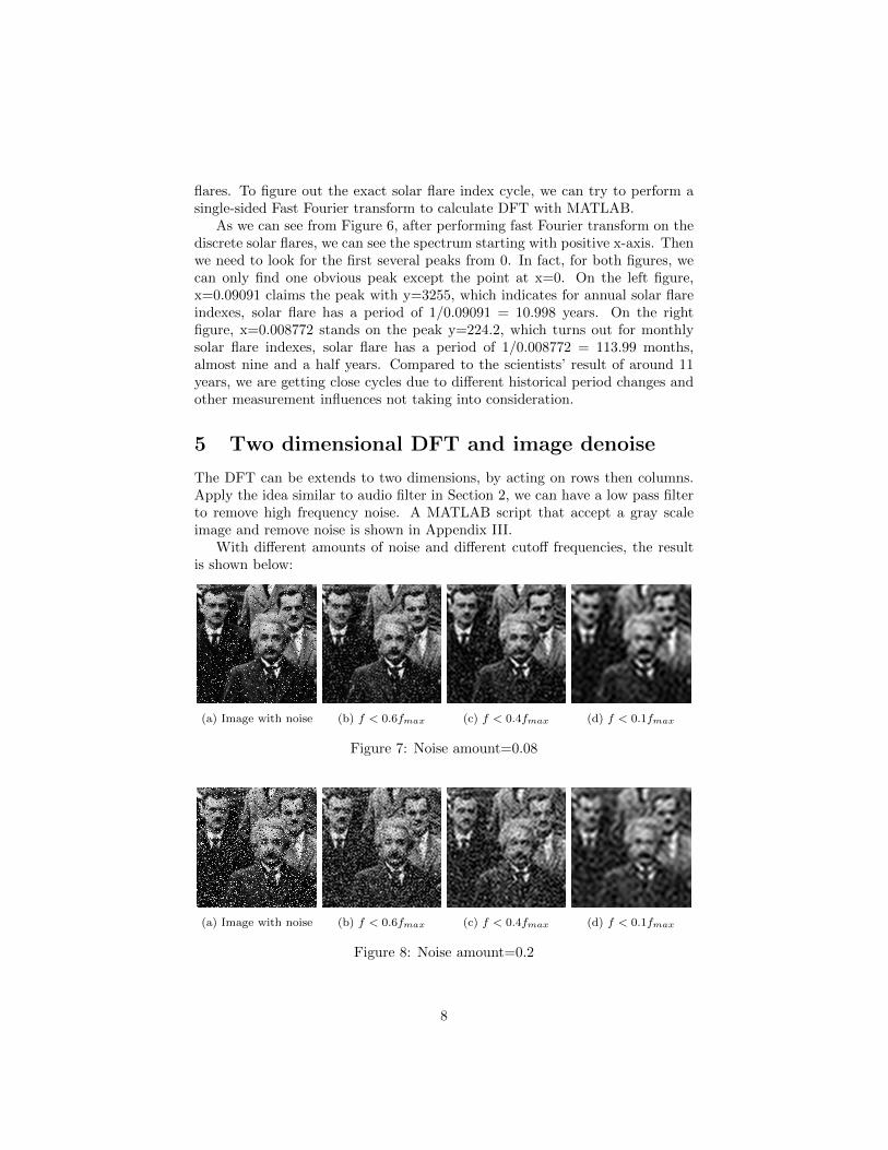
flares. To figure out the exact solar flare index cycle, we can try to perform asingle-sided Fast Fourier transform to calculate DFT with MATLAB.

As we can see from Figure 6, after performing fast Fourier transform on thediscrete solar flares, we can see the spectrum starting with positive x-axis. Thenwe need to look for the first several peaks from 0. In fact, for both figures, wecan only find one obvious peak except the point at x=0. On the left figure,x=0.09091 claims the peak with y=3255, which indicates for annual solar flareindexes, solar flare has a period of 1/0.09091 = 10.998 years. On the rightfigure, x=0.008772 stands on the peak y=224.2, which turns out for monthlysolar flare indexes, solar flare has a period of 1/0.008772 = 113.99 months,almost nine and a half years. Compared to the scientists’ result of around 11years, we are getting close cycles due to different historical period changes andother measurement influences not taking into consideration.

5 Two dimensional DFT and image denoise

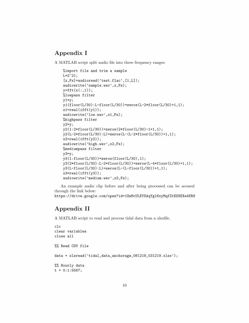
The DFT can be extends to two dimensions, by acting on rows then columns.Apply the idea similar to audio filter in Section 2, we can have a low pass filterto remove high frequency noise. A MATLAB script that accept a gray scaleimage and remove noise is shown in Appendix III.

With different amounts of noise and different cutoff frequencies, the resultis shown below:

(a) Image with noise (b) f < 0.6fmax (c) f < 0.4fmax (d) f < 0.1fmax

Figure 7: Noise amount=0.08

(a) Image with noise (b) f < 0.6fmax (c) f < 0.4fmax (d) f < 0.1fmax

Figure 8: Noise amount=0.2

8

References

https://www.ngdc.noaa.gov/stp/solar/solarflares.htmlhttps://tidesandcurrents.noaa.gov/waterlevels.htmlhttps://oceanservice.noaa.gov/education/tutorial tides/tides05 lunarday.htmlhttps://oceanservice.noaa.gov/education/tutorial tides/tides06 variations.html

9

Appendix I

A MATLAB script split audio file into three frequency ranges:

%import file and trim a sample

L=2^21;

[x,Fs]=audioread(’test.flac’,[1,L]);

audiowrite(’sample.wav’,x,Fs);

y=fft(x(:,1));

%lowpass filter

y1=y;

y1(floor(L/30):L-floor(L/30))=zeros(L-2*floor(L/30)+1,1);

x1=real(ifft(y1));

audiowrite(’low.wav’,x1,Fs);

%highpass filter

y2=y;

y2(1:2*floor(L/30))=zeros(2*floor(L/30)-1+1,1);

y2(L-2*floor(L/30):L)=zeros(L-(L-2*floor(L/30))+1,1);

x2=real(ifft(y2));

audiowrite(’high.wav’,x2,Fs);

%mediumpass filter

y3=y;

y3(1:floor(L/30))=zeros(floor(L/30),1);

y3(2*floor(L/30):L-2*floor(L/30))=zeros(L-4*floor(L/30)+1,1);

y3(L-floor(L/30):L)=zeros(L-(L-floor(L/30))+1,1);

x3=real(ifft(y3));

audiowrite(’medium.wav’,x3,Fs);

An example audio clip before and after being processed can be acessedthrough the link below:https://drive.google.com/open?id=1OnMcULEYXAqYgl6xyMqfZtESXEXe4KR9

Appendix II

A MATLAB script to read and process tidal data from a xlsxfile.

clc

clear variables

close all

%% Read CSV file

data = xlsread(’tidal_data_anchorage_061218_031219.xlsx’);

%% Hourly data

t = 0:1:5567;

10

L = 5567;

Fs = 1; % Sampling frequency in hours

f = Fs*(0:(L/2))/L;

Y = fft(data(:,1));

P2 = abs(Y/L);

P1 = P2(1:(L/2)+1);

P1(2:end-1) = 2*P1(2:end-1);

figure(1);

plot(f,P1, ’k.’)

figure(2);

plot(t,data(:,1),’r.’);

Appendix III

A MATLAB script add noise to an image and then remove the noise by usingFFT:

%load an image

M = imread(’test.jpg’);

n = size(M);

%add noise to the image

M = imnoise(M,’salt & pepper’,0.08);

imwrite(M,’noise.jpg’)

%denoise in one direction

for i=1:n(1)

x = fft(M(i,:));

for j = 1:length(x)

if (j>floor(length(x)/6))

&& (j<length(x)-floor(length(x)/6))

x(j) = 0;

end

end

M(i,:) = real(ifft((x),n(2)));

clear x

end

%denoise in the other direction

11

for i=1:n(2)

y = fft(M(:,i));

for j = 1:length(y)

if (j>floor(length(y)/6))

&& (j<length(y)-floor(length(y)/6))

y(j) = 0;

end

end

M(:,i) = real(ifft((y),n(1)));

clear y

end

%save denoised image

imwrite(M,’denoise.jpg’)

12