Embed Size (px)
Citation preview

NTIA-REPORT-79-30
Signal Level Distributions and
Fade Event Analysesfor a 5 GHz Microwave Link
Across the English Channel
D.R. WortendykeA.P. Barsls
R.R. Larsen
u.s. DEPARTMENT OF COMMERCEJuanita -M. Kreps, Secretary
Henry Geller, Assistant Secretaryfor Communications and Information
October 1979

TABLE OF CONTENTS
ABSTRACT
Pag~
1
1.
2.
3.
4 •
5.
6 •
7.
8 •
INTRODUCTION
MICROWAVE SYSTEM DESCRIPTION ANDIMPLEMENTATION
DATA COLLECTION EQUIPMENT
MEASUREMENT RESULTS
4.1 Signal Level Distributions4.2 Comparisons with Fading Models4.3 Fade Event Durations
APPLICABILITY OF RESULTS TO SYSTEMS INOTHER AREAS
CONCLUSIONS
ACKNOWLEDGEMENTS
REFERENCES
1
2
4
8
81113
20
22
23
23
Figure 1.
Figure 2.
Figure 3.
Figure 4.
Figu~e 5.
Figure 6.
Figure 7.
Figure 8.
Figure 9.
LIST OF FIGURES
Location map fb~ 5 GHz microwave link.
Terrain profile for 5 GHz microwave link.
Data flow diagram for RSL-2 rec6rdingsystem.·
Sample of digital strip chart recording
Received signal level distributions(all data).
Comparison of measurement results withCCIR signal level predictions.
Example of multiple fades within asingle fade event.
Fade event duration distributions forwinter time blocks.
Fade event duration distributions' forsummer time blocks.
2
3
5
7
9
12
15
16
17
Figure 10. Fade event duration distributions forall hours. 18
iii


Table 1.
Table 2.
Table 3.
LIST OF TABLES
Sample Printout for Hourly "Quick-look"Analysis
Path and Equipment Parameters
Fade Event Duration Statistics for Path~
A and B, Swingate - Houtem
v
Page
6
10
19

SIGNAL LEVEL DISTRIBUTIONS AND FADE EVENTANALYSES FOR A 5 GHz MICROWAVE LINK
ACROSS THE ENGLISH CHANNEL
D.R. Wortendyke*, A.P. Barsis*, and R.R. Larsen**
This report describes instrumentation for fadingstudies and measurement results over an 88-kmmultiple-diversity line-of-sight microwave linkacross the English Channel operating in the4 to 5 GHz frequency range. Signal level andfade, duration statistics derived from the measurements are compared with CCIR models. It is foundthat median fade duration tends to be less thanestimates from the CCIR models.
Key words: Microwave fading, multiple diversityreceivers, 5 GHz signal levels, automatic signal monitoring.
1. INTRODUCTION
The Ins,titute for Telecommunication Sciences (ITS) of the
National Telecommunications and Information Administration
u.s. Department of Commerce was tasked in 1972 by the U.S. AirI
Force Communications Service (AFCS) to develop automated test and
acceptance procedures and equipment to simplify and accelerate
the collection of test and performance data from Defense Communi
cation Systems (DCS) microwave links. Emphasis was first on
measurement and analyses of received signal level data. Initially,
ITS developed a calculator-based instrument (RSL-l) in 1973,
which was used on the "SCOPE" conununication links in Germany and
as a measurement-analysis tool at AFCS Headquarters. Later, a
more sophisticated instrument for received signal level (RSL)
measurements and analysis was developed by ITS. The present
report deals with the utilization of this instrument in a long
term study and evaluation of propagation effects on a 'multi
diversity microwav~ link across the English Channel between
*The authors are with the National Telecommunications and Information Administration, Institute for Telecommunication Sciences,u.S. Dept. of Conunerce, Boulder, CO 80303.
**The author is with the' l842nd Electronics Engineering Group,United States Air Force, Scott Air Force Base, IL 62225.

terminals near Dover, England, and Houtem, Belgium. This link is
88 km long (with 65 km over water), and operates in the 4 to 5
GHz frequency range. It is a portion of the DCS European network,
and has "been carrying traffic since mid-1974.
This report presents first a description of the path, its
implementation, and a brief out Li.ne of the RSL-2 instrumentation.
Next is a discussion and analysis of measurement results from a
I-year operating period. Statistics of signal level and fade
events are presented, and the results will also be evaluated for
applicability to similar links.
2. MICROWAVE SYSTEM DESCRIPTION AND IMPLEMENTATION
As shown in Figure 1, the western terminal of the 88-km
link is at Swingate, near Dover, England, on top of the White
Cliffs. The eastern terminal is approximately 19 km inland from
the Channel coast near Houtem,Belgium. The path profile with
antenna positions, heights above mean sea level (in meters), and
a representation of the sea surface for two values of the
effective earth radius factor, k, is shown in Figure 2. Anten
nas A and B at each terminal are 4.6 m parabolic reflectors, and
antennas C and Dare 3.7 m parabolic reflectors.
ENGLAND
LONDON
-
FRANCE
-BRUSSELS
BELGIUM
PARIS-Figure 1. Location map for 5 GHz microwave link.
2

V>0::::L.LJ
~ ~ A 244~ 230 AH ~ B 235
221 I ~
....J
L.LJ 184>;
~ d ----- ~-- ~K = 2/3e:t: 14 1 C ---- -----I..LJ -----V> ~ 1 /1 ---- -----
~ WHITE, /' ---- _~ CLIFFS OF
DOVERw ~ \/ ~ ~ - ~HC 41
o
~ ~ K=oo • db ~V> I I I I I I I I I I I I 3~ 0 10 20 30 40 50 60 70 80 90(!' 3 74 88
~ SWINGATE DISTANCE IN km DUNKERQUE HOUTEM::c ENGLAND FRANCE BELGIUM
Figure 2. Terrain profile for 5 GHz microwave link.

The design considerations for the multiple diversity system
wer~ described in detail by Zebrovitz (1975). For sub-refractive
and normal conditions (2/3 ~ k ~ 4/3), dual diversity operation
is provided by paths A and B. For the top path A, clearance
amounts to approximately the 11th or 12th Fresnel zone for
k = 4/3, but it is only a small fraction of the first Fresnel I
zone (less than 0.1) for k = 2/3. Under these -conditions, the
lower paths (C and D) contribute relatively little to the quad
ruple diversity combiner input since direct line of sight for
these lower paths is blocked by the sea surface. However, when
signals from the upper antennas are subject to severe multi~ath
fading because of superrefractive conditions (k > 4/3), the lower
paths C or D may be within the superrefractive layer with very
little attenuation. They would then be expected to provide the
principal contribution to the'combiner. The lower path C, as an
example, becomes grazing for k = 1.82.
Two of four transmitters are used as standbys at any
specific time, and up to four usable signals at a time are
provided to the combiner. It was anticipated that this design
would fulfill the performance requirements in terms of signal
level and noise power ratio for at least 99.99% of the time.
3. DATA COLLECTION EQUIPMENT
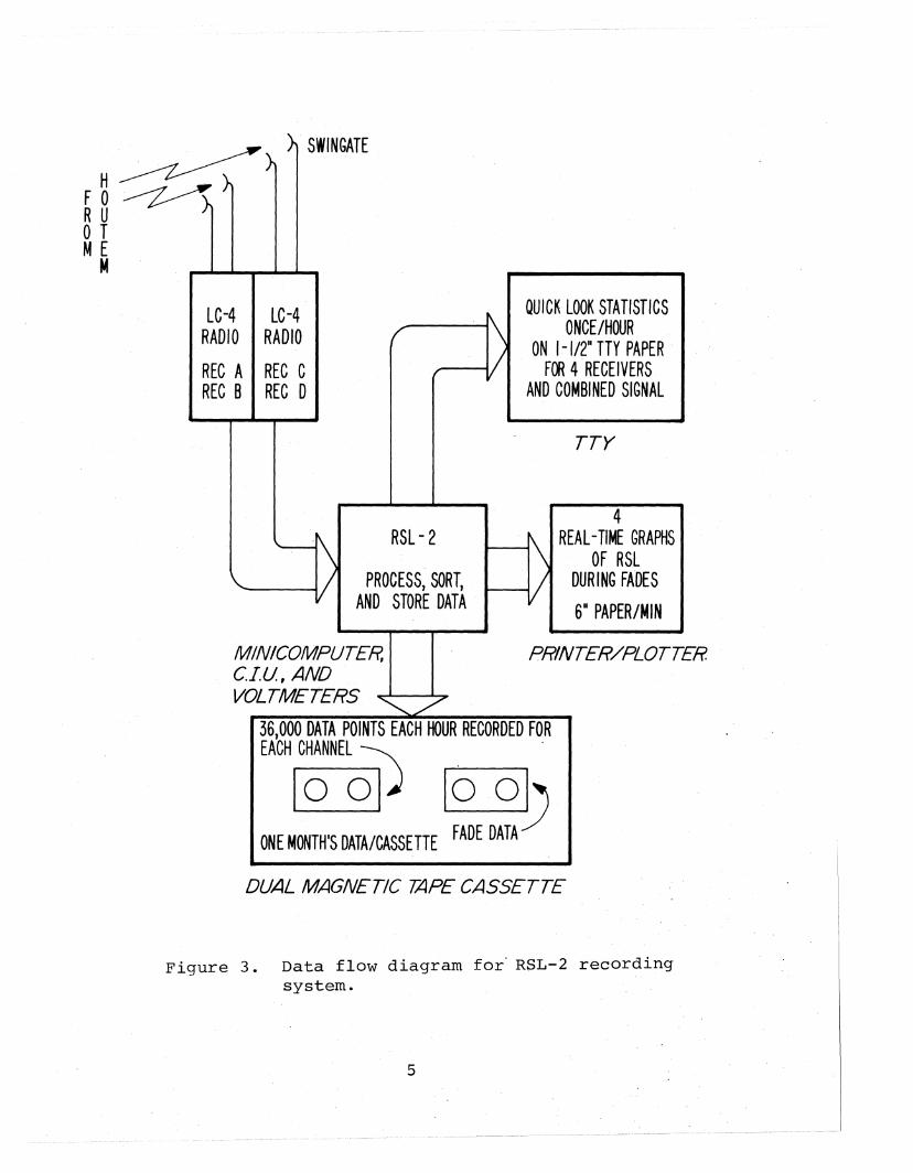
The RSL-2 measurement instrument is a minicomputer-con
trolled device designed to handle great quantities of time
variant data. The conceptual operation is shown in Figure 3; it
is controlled by software programs core-~esident in the 24-k word
memory. Fbur dc vo~tages, prop6rtional to the received signal
levels from each of four receivers, are measured every 0.1 s by a
12-bit A-D converter. The mini-computer sorts each of the four
measurement values against a stored calibration curve for the
particular receiver and then places the data in a histogram with
20 partitions that are equally spaced across the receiver dynamic
range. Once per hour the histograms are stored with a date-time
group and the process begins again. A five-point cumulative dis
tribution (signal levels in dBm exceeded for 10%, 50%, 90%, 99%,
4
F~~}R UoTME
M
} } SWINGATE
LC-4 LC-4RADIO RADIO
REC A REC CREC B REC D
QUICK LOOK STATISTICS" ONCE/HOUR
/ON 1-1/2" TTY PAPER
,,-------1 FOR 4 RECEIVERSAND COMBINED SIGNAL
TTY
RSL - 2
PROCESS, SORT,AND STORE DATA
4I------t~ REAL-TIME GRAPHS
i \ OF RSL.---..V DURING FADES
611 PAPER/MIN
MINICOMPUTER, PRINTER/PLOTTER.C.I.u., ANDVOLTMETERS ",,/,
36,000 DATA POINTS EACH HOUR RECORDED FOR
EACHICOHA.NNELO~100b
ONE MONTH'S DATA/CASSETTE FADE DATA
DUAL MAGNETIC TAPE CASSETTE
Figure 3. Data flow diagram for· RSL-2 recordingsystem.
5

and 99.9% of the hour) for each of the histograms is also printed
out each hour. This is called a quick-look analysis and an
example is shown in Table 1. Also, a simulated distribution for
all four channels is computed by additive combination of signal
power and listed in the right hand column of the printout; it
represents optimum system performance, provided all radio hardware
(particularly the combiner circuitry) is properly functioning and
adjusted. If the signal level'fades below a p~e-set threshold
for the normally line-af-sight upper two paths on receiver A or
B, a fUlly annotated, cal~brated, digital, 4-channel strip chart
is printed on a printer-plotter for the duration of the fade plus
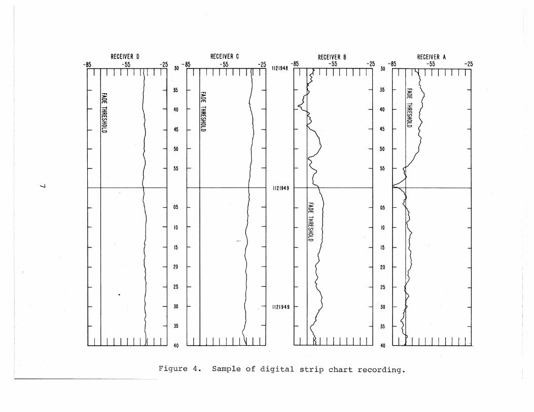
a pre-set I-min interval.* Chart speed is 6 in/min. An example
is shown in Figure 4 that also illustrates the relatively high
and steady signals over the lower paths C and D occurring fre
quently when the signal over paths A and B is in deep fades.
Table 1. Sample Printout for Hourly "Quick-look"Analysis - Distribution Levels in dBm
% Time That Recvr A Recvr B Recvr C Recvr D CombinedLevel isExceeded
10%50%90%99%99.9%
-43 -40 -34 -37 -31-46 -43 -37 -40 -34-55 -58 -40 -43 -37-70 -70 -52 -46 -37-79 -82 -55 -49 -40
The measured data are stored in a buffer for 10 s, and the
output to the printer-plotter is taken from the oldest of the
buffered data. Thus, the displays start prior to the leading
edge of the fade. At the end of the fade interval (fade
duration plus 1 min) the histograms, with starting and ending
times, are recorded in a file on a magnetic tape cassette.
Hourly data histograms and calibrations are recorded periodi
cally on tape for later evaluation. Each of these cassette
tapes can store one month of data. The fade tape capacity is
340 "events" regardless of duration.
*The effect of this delay on fade duration statistics will bediscussed in Section 4.3.
6
..,.,:> I ~ 05c::;,f'T'1
--f::I::::crT'1 I --I 10en::I:c::>r-c::::;:)
I I15
20
25
1121949 r II l 30
35·
40
35
30
10
15
25
05
20
.40
RECEIVER C RECEIVER B RECEIVER A-25 -85 -55 -25 1121948 -~5i -55 -25 -85 -55 -25
30 , i i i i i i i i i Ii i , i C i i i i i i i i , 30
35 ~ I..,., - 35 ..,.,:>
:> c::;,c::;, f'T'1f'T'1
--f
40 t- I~ 40::I::::c
:;::ID f'T'1rTI enen ::I:::I: c::>c::> r-
45 r- 45c::;,
t::::'
50 50
55 55
1121949
>orTI
--f::x::::c,.."en:x:c::>rt::::'
RECEIVER 0-85 -55
....J
Figure 4. Sample of digital strip chart recording.
Data acquisition and sorting is done in about 10 ms, leav
ing 90 ms between clock ticks available for other tasks such as
further processing when the teleprinter is not actually printing
any data. Processed data include a histogram and cumulative
distributions of received signal levels for any hour, day, month,
or fade period. Any set of calibration voltages maybe read
from the monthly tape for quality assurance checks of system
performance.
4. MEASUREMENT RESULTS
Signal level distributions and fade event statistics were
obtained over the period from mid-July 1974 to the beginning of
June 1975. During this time, the radio system and the RSL-2
equipment were operating for approximately 3650 hrs distributed
over the entire year so that all seasons are represented. This
constitutes the data base for the analyses of signal level
'distributions and fade duration.
4.1 Signal Level Distributions
Figur~ 5 is a plot of instantaneous signal level distribu
tions for all four receivers obtained from the RSL-2 equipment
at the rate of 10 data points per second. Approx.lrnat.eLy
130 x 106 samples for each receiver are represented here. The
data are p~otted on Rayleigh paper and compared with the
theoretical Rayleigh distribution. Qualitatively, the approxi
mation appears to be good for the data from the line-of-sight
paths (receivers A and B) suggesting mUlti-component multipath as
the principal cause of fading. The data from receivers C and D
deviate substantia~ly from the Rayleigh distribution, and the
effect of super refraction during small percentages of time is
quite evident from the steep rise of the curves toward the free
space level of -32.9 dBm for small percentages of time. The graph
also shows the calculated distribution for all signal powers com
bined additively (see the, discussion in Section 3 in conjunction
with Table l)~ The apparent system performance improvement is
about 12 dB for 99.9% of the time over the performance of a single
8

6
""",
"0,
RECEIVER B
'<,~""l:i
"~ RAYLEIGH SQUARED
" ....,'............ _--
RAYLEIGH~
99.8 99.999.95 99.98 99.99 99.995 99.998 99.999 99.9995
--~ ....j "' "'~"' "
98 99
DATA TAKEN BETWEEN MID 1974 AND MID 1975DATA RATE = 10/SECOND
II I I
,x
"-,
RECEIVER D~'x-,, ,
5 :20 40 50 60 70 80 90 95
\x\\x\
\x,
-80 I I ~ JIlt, ), > J
COMBINER OUTPUT COMPUTEDFROM INSTANTANEOUS SAMPLES
I I...., I
':::...::.......~o
-50 I ,\ ~ "' . "
-40 I >5t ~ ~
-60 I '.... ',,= \: "" '" .... c
EaJ"C
.::::Jena:--'LU>LU--'--'~ «2:t!Jen0LU>WULUa:
% OF TIME ORDINATE IS EXCEEDED
Figure 5. Received signal level distributions (all data).

line~of-sight path. This combined distribution follows the
"Rayleigh squared" curve as postulated by White for uncorrelated
fading (White, 1970).
Note that this graph represents the distribution of
instantaneous signal level values and should not be comp~red
with calculated distributions of hourly medians that would tend
toward a normal distribution.
From the system parameters (Zebrovitz, 1975), the received
signal level corresponding to line-of-sight transmission through
the atmosphere without the effects of reflections or multipath
is -32.9 dBm. The parameters are listed in Table 2 below.
Figure 5 shows that the median ~eceivedsignal levels· over the
measurement period differ from this value: they are -38.7 dBm
for receiver A, and -41.3 dBm for receiver B. This discrepancy
as well as the difference between the results from the two
receivers may be caused by uncertainties in equipment param
eters, antenna alignment, and possibly by path or atmospheric
parameters not considered in the calculations.
Table 2. Path and Equipment Parameters
Pathlength: 87.84 km
Carrier frequency (mean forreceivers A and B):
Free-space basic transmission loss:
Antennas:
Antenna gain:
Transmitter power:
Estimated wave guide andrelated losses:
Average atmospheric absorption:
Estimated average annual meantemperature:
10
4.908 GHz
145.1 dB
4.57 m (15 ft)paraboloids
44.8 dB (relative toisotropic)
6.3 W (+38 dBm)
14.5 dB
0.8 dB
10 0 C
4.2 Comparisons with Fading Models.
Prediction models for fade ~epth distributions over micro
wave line-of-sight links have been developed by a number of
workers (Barnett, 1972; Morita, 1970). At the XIV Plenary
Assembly of the CCIR, use£ul formulations of these models were
adopted and included in Report 338-3 (CCIR, 1978). This formu
lation is based on a general expression with specific constants
for Japan, Northwest Europe, and the united States, and is in
tended to be valid for the "worst fading month". Consequently,
the probabilities of fade occurrence calculated in this manner
should be converted from "worst month" to "all year" for compar
ison with the data described here. Vigants (1975) suggests a
procedure for doing this ca~culation as a funct.i-on of the
annual mean temperature over the path.
Using the applicable path parameters from Table 2, the
model distributions were calculated in accordance with the
CCIR formulation for Northwest Europe and plotted together
with data points for receivers A and B as shown in Figure 6,
but only those for deep fades (at least 20 dB below the yearly
measured median) where the Rayleigh d~stribution postulated
by the models (CCIR, 1978) is most applicable. Agreement between
the data and the model distributions is reasonable but illustrates
the uncertainty in extrapolating from "worst month" to "all year"
on the basis of an annual mean temperature only. In fact, the
data tabulations do not suggest a particular "worst month";
fading is~distributed rather uniformly over the year.
Zero reference for the ordinate in Figure 6 is the mean
of the yearly median signal levels derived from the receiver
A and receiver B measurements (see Figure 5).
Additional calculations have shown that the model given
in CCIR Report 338-3 (1978) is not applicable to this path
since it greatly overestimates fading occurrence. This is
not surprising since this model was derived primarily from dataI»
for much shorter overland paths in the midwestern united States.
11

-10
..:z: 10es~LU:E:
~LU0:::
~ 20<CLU:IE
:c:>--J
~ 30
40
o ENGLISH CHANNEL DATA (RECEIVER A)
o ENG LIS H CHA'N NELOATA (R ECEIVERB)
CCIR worst month"~D,
o 0
c
0.99 0.9 0.5 0.1 0.01 0.001 0.0001 0.00001
FRACTION OF TIME, P, BELOW LEVEL
Figure 6. Comparison of measurement results withCCIR signal level predictions.
12
4.3 Fade Event Durations.
As explained in Section 3, the RSL-2 equipment automat
ically acquires, stores, and calculates statistics of fade
event duration at pre-set received signal levels. Datawere
obtained throughout the measurement period for receivers A
and B; i.e., for the line-of-sight paths between the high
antennas (see Figure 2). The pre-set fade threshold for all
data was -75 dBm which is 35 dB below the average of the
all-year signal level medians for the two receivers.
The recording and analysis routine inherent in the RSL-2
equipment emphasize&what we choose to call "fade events"
rather than individual fades. The start of a fade event is
defined as that instant when the received signal level from
either receiver A or receiver B drops below the -75 dBm
threshold. The computer then sorts and stores signal level
histograms for all four receivers until one minute after sig
nals from receivers A and B have both risen above the thres
hold levels and have remained there. It records the total
elapsed time for receivers A and B signals at and below the
threshold level, and the total length of the fade event cor
recting for the one-minute time lag. A fade event may include
individual fades on both channels.
The time lag was introduced to allow for limitations. in
the peripheral hardware (particularly the tape drive); the
recording mechanism cannot completely follow a nurnberof short
fades in rapid succession. This limitation introduces a
significant bias (against short fades) in the statistical
evaluation of the p~esent data.
Thus, any additional deep fa~e below the threshold level
that occurs within the one-minute period after the first rise
above the threshold is not evaluated separately, but recorded
as part of the original fade. Consequently, any number of
short fades separated by less than one minute are lumped into
one single longer fade event. Processing methods inherent in
the computer and used for the original data recording methods
13

make it impossible to recover the number and durations of the
individual fades when separated by less than one minute.
Inspection of available graphic printouts suggest that many
of the fades w~re indeed isolated; i.e., separated by at
least one minute. However, Figure 7 shows an example of
multiple fades of short duration (about 1 s or less) within
a single fade event lasting approximately 45 seconds.
Figures 8, 9, and 10 show cumulative distributions of fade
event durations obtained in the manner described above. These
distributions are plotted on a log-hormalgrid; i.e. the absis
sas are linear in terms of 10 times the logarithm (to the base
10) of the fade event durations in seconds. Because of the
bias introduced by the recording method, the total number of
individual fades is greater than the number of fade events and
and their duration may be appreciably shorter as will be shown
later. The distributions are categorized into "time blocks" for
winter (Figure 8) and summer (Figure 9) which were introduced
originally by Norton, et ale (1955) to evaluate tropospheric
propagation data.* These categories provide an indication of
diurnal and seasonal changes in the fade event duration distri
butions. Summary statistics for fade event durations are given
in Table 3 below. Similarly, overall cumulative distributions
for all hours - winter, all hours - summer, and all hours of the
year are shown in Figure 10 with the statistics also listed in
Table 3. It is quite evident that the median fade event durations
are substantially greater in winter than in summer. However,
there are almost twice the number of fade events in summer than
in winter (781 versus 414). Nevertheless, the total time in
fades of 35 or more dB below the yearly median signal level is
still greater in winter than in summer.
*Thewinter time block comprises November through April, and thesummer time block May through October.
14

-25RECEIVER A
-55
55
50
-25 -85
15
Received Sig no I Leve I (dBm)Houtem to Swingote
RECEIVER B-55
05
10
15
20 ---t::::I:
-n ::x:J
::J> rT1
c::::J cr»rT1 25 :::c
c:::>--f
r-::::I:
c::::J
::::tJrT1
30cr»::cc:::>r-c::::J
35
40
45
Figure 7. Example of multiple fades within a singlefade event.
2141719
-852141718

...... , .... ...... ......
MEDIANS
Sec0- 6 6.06-13 12.013-18 6.918-24 9.0
"~~.
.~:~ll.. r- ," -.. ,~, <.
<, ." ••••
" " ." ". " "--, \".
" \ ".
. " '."'.~ -.",. -.
.,~ ...\~:- ..,-.
~.'.\ \ ".\ \'.
',".~~'-.
' ..
.18'?t1",.~
.""0'8
WINTER MONTHS
1000 , iii (. iii iii iii I I I i
,"",100fn-ac::0c.,)CI,)
tn...........
~c::::>t- 10<0::::::::>~
t-:IELU:>LU
I-' LLJO't ~
ceLa-
0.1
0.01 0.1 2 10 20 30 40 50 60 70 80 90 98 99
PERCENT OF EVENTS FOR WHICH ORDINATE IS EXCEEDED99.9 99.99
Figure 8. Fade event duration distributions for winter time blocks.

1000 i I I Iii iii iii Iii i ,
100.....-..-.tn-aC0UCI)tn.........,
:zc::::>t= 10<Cc:::::::>~
t--z:
I--JLLJ
-......]::::-LLJ
LU~
<CLa-
-0.1
. I.>'V,/
" /&/8.... ~A" ' •
.~ "................. <,
~~.~.", ...........
-~"".:.:--'.'. , \
8~ij""" . '<\\ .
. '" \ \. "' '\
0. ~'.\.... '-0.. ,.'. ,~
". \\~'. v
'. \\...\'"".','".... \ '\
0\ .00' \
00",<•."" .,.. "'.SUMMER MONTHS "":':~ ..
'~..
MEDIANS
Sec0-6 3.166-13 1.46
13-18 - 2.018- 24 . 2.57
0.01 0.1 2 10 20 30 40 50 60 70 80 90 98 99PERCENT OF EVENTS FOR WHICH ORDINATE IS EXCEEDED
99.9 99.99
Figul~e 9. Fade event duration distributions for summer time blocks.

1000 I I · I K I I I I I I I I I I I I I
Sec8.122.243.16
MEDIANS
WINTERSUMMER
ALL YEAR
'.
ALL YEAR
S'(/~'~Ep
<, <,rr ~#;<, , ' ••-1« ~J:
<, ' .. {s q,"" . ·f4>, .
"" ........ e." ." ' ." .<, ", ".<, -, '.
<, "'.<, ".
<, \'.<. \ ....
~""
"'.,,,, .-, ')-.., '.~
" .\.... -. CC/tf\<..· ~ "Ot/,l"
,. ~J (-, ". ,/81...,
-, '. <, a)-, '.-, '.
-, '.,e.-.'."".".'e.
100
..--...en-ac::<::)
uQ)
tn............
:z10c:::>t--<Cet:::~
~
I-' t--co :iii!:
LU::::-LU
LUc::::.<LL..
0.1
0.01 0.1 2 10 20 30 40 50 60 70 80 90 98 99
PERCENT OF EVENTS FOR WHICH OROI NATE IS EXCEEDED99.9 99.99
Figure 10. Fade event duration distributions for all hours.
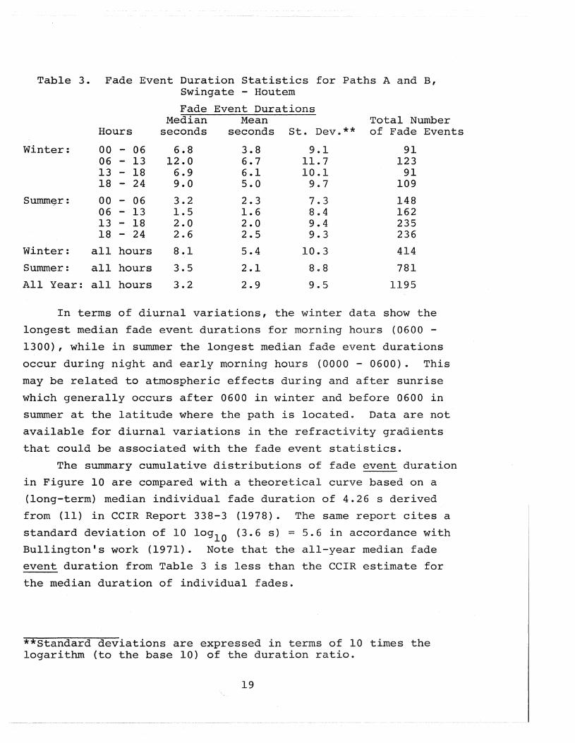
Table 3. F.ade Event Duration Statistics for Paths A and B,Swingate - Houtem
Fade Event DurationsMedian Mean Total Number
Hours seconds seconds St. Dev. ** of Fade Events
Winter: 00 - 06 6.8 3.8 9.1 9106 - 13 12.0 6.7 11.7 12313 - 18 6.9 6.1 10.1 9118 - 24 9.0 5.0 9.7 109
Summ~r: 00 - 06 3.2 2.3 7.3 14806 - 13 1.5 1.6 8.4 16213 - 18 2.0 2.0 9.4 23518 - 24 2.6 2.5 9.3 236
Winter: all hours 8.1 5.4 10.3 414
Summer: all hours 3.5 2.1 8.8 781
All Year: all hours 3.2. 2.9 9.5 1195
In terms of diurnal variations, the winter data show the
longest median fade event durations for morning hours (0600
1300), while in summer the longest median fade event durations
occur during night and early morning hours (0000 - 0600). This
may be related to atmospheric effects during and after sunrise
which generally occurs after 0600 in winter and before 0600 in
summer at the latitude where the path is located. Data are not
available for diurnal variations in the refractivity gradients
that could be associated with the fade event statistics.
The summary cumulative distributions of fade event duration
in Figure 10 are compared with a theoretical curve based on a
(long-term) median individual fade duration of 4.26 s derived
from (11) in CCIR Report 338-3 (1978). The same report cites a
standard deviation of 10 logI 0 (3.6 s) = 5.6 in accordance with
Bullington's work (1971). Note that the all-year median fade
event duration from Table 3 is less than the CCIR estimate for
the median duration of individual fades.
**Standard deviations are expressed in terms of 10 times thelogarithm (to the base 10) of the duration ratio.
19

We have already noted that individual fades for the
Swingate - Houtem path are frequently shorter in duration than
fade events. Although it is not possible to recover the
statistics of individual fades from the cassette records, the
comparison of fade event durations with signal level distribu
tions for the -75 dBm threshold level permits an estimation of
the relation between the number and the duration of individual
fades and fade events. A sample analysis was conducted for
typical summer and winter data; also, some of the fade event
strip charts are available for inspection. The example shown in
Figure 7 is somewhat extreme since there are 8 individual fades,
each lasting about 1 s or less, for the single 47.3 s fade
event on receiver A.
This sample analysis resulted in median values of 2.3 indi
vidual fades per fade event for the summer example, and 2.1 for
the winter example. Consequently, on the average there will be
at least twice as many individual fades as fade events. Also,
the median duration of individual fades is likely to be not more
than about one-half of the median of the fade events. Even in
the absence of information permitting more complete statistical
analyses, it would appear that the CCIR model tends to over
estimate median fade duration for this path, and possibly for
other paths of this type; i.e., long over-water links in theI
4 to 5 GHz frequency range. A comparison of the slopes for the
theoretical and the measured distributions shown in Figure 10
is not appropriate because of the bias introduced by the measure
ment methods.
5 . APPLICABILITY OF ~ESULTS TO SYSTEMS IN OTHE'R AREAS
The microwave communication link evaluated in this report
is somewhat atypical because of its length (88 km) and environ
ment (across water). It is, however, possible to apply the
results to other over-water and coastal areas since fading
characterisitcs are related to terrain and atmospheric strati
fication. A measure of the latter are statistics o£ refractiv
ity gradients. Detailed, gradient statistics for the exact path
location during the measurement period could not be obtained.
20

The points closest to the path for which long-term cumulative
distributions of the refractivity gradients are available are
Cardington, England (north of London), and Brussels, Belgium
(Samson, 1975). At these two locations, ground-based super
refractive layers (N-units/km < -40) at least 100 m thick occur
for 60 to 70% of the observations (twice daily at Brussels and
four times daily at Cardington). Also, gradients more negative
than -250 N-units/krn were observed for approximately 0.1% of the
occurrences at Cardington in the groundbased layer up to 500 m
above ground.
The compilations of gradient statistics prepared by
Samson (1975, 1976) illustrate the preponderance of super
refractive gradients in most coastal locations in the United
States. Examples of locations for which such gradients in the
ground-based IOO-m layer occur during at least 25% of the
observations are Anchorage and Barrow, Alaska; Long Beach,
Oakland, and San Diego, California; Key West and Miami, Florida;
Washington, D.C.; Hila, Hawaii; Caribou, Maine; New York, N.Y.;
Cape Hatteras, ,North Carolina; Seattle, Washington; and Browns
ville, Texas. Even ducting gradients are relatively frequent
at these locations with the highest incidence found at Hilo and
Cape Hatteras (>9%).
It may therefore 'be concluded that the results of the
measurement program described here may be applicable to most
coastal areas in North America and to links in Pacific Island
chains. We must remember, however, that the path discussed
here is unusually long for a line-of-sight link, and that the
antennas for ,the line-of-sight situation are by necessity high
above the surface.
The results could also be applied to some inland locations
in continental climates where the path extends over relatively
smooth terrain and super-refractive gradients exist for appreci
able fractions of the observations. Examples, during the
summer months, are 'Denver, Colorado; Bismarck, North Dakota;
21
and Dayton, Ohio. However, terrain influences the homogeneity
of the gradient structure, and a careful study of the terrain
is essential in these cases.
6. CONCLUSIONS
The.purpose of this study is to check the measurement
results against available prediction models, particularly those
recommended by the CCIR. Agreement between predicted signal
level distributions and those derived from the measurement~ is
fair in the deep fading region where the CCIR model applies.
The results, if representative of a full year, do not confirm
the- validity of extrapolating from worst month to all year on
the basis of annual mean temperature as suggested by Vigants
(1975). However, the maritime climate characteristics of the
path environment tend to lessen seasonal changes and make the
concept of a "worst month" less applicable.
Because of the limitations in the measurement techniques,
precise statistics of individual fades could not be obtained.
From the analyses and reasoning described in Section 4, it appears
that the median duration of individual fades is not more than
approximately one-half of that expected from available fade event
models. Total fade event durations are longer in winter than in
summer while the number of fade events is larger in summer.
Assuming that fading characteristics are primarily a func
tion of refractivity gradient statistics, the results of the
measurement program are applicable almost universally over water
or smooth coastal terrain since the gradient distributions for
the area of the path are not unique. Because of its length,
however, the path is not typical of overland communication
links. Since the super-refractive gradients that favor fade
events occur frequently even inland in continental climates,
allowance for substantial fading must be made for long links
unless the terrain can be expected to inhibit homogeneous
stratification over the path area.
Finally, the measurement results confirm the usefulness of
the original design concept for this path. Because of the link
22

length and inadequate clearance (under generally accepted
standards), extensive fading exists on the nominally line-of
sight paths between the upper antennas. The quadruple diver
sity system utilizing paths between lower antennas that are
normally blocked, but can become active during'ducting condi
tions, appears to work well, and_insures adequate communication
reliability. It is reasonable to expect that similar designs
will work equally well in most coastal or maritime environ
ments where super-refractive gradients exist for large fractions
of the time.
7. ACKNOWLEDGEMENTS
The authors wish to thank D.D. Crombie and H.T. Dougherty
for their careful review and pertinent suggestions.
8 . REFERENCES
Barnett, W.T. (1972), Multipath propagation at 4, 6, and
11 GHz, Bell System Tech. J., 51, No.2, 321 - 361.
Bullington, K. (1971), Phase and amplitude variations in
multipath fading of microwave signals, Bell System
Tech. J., 50, No.6, 2039 - 2053.
CCIR (1978), Propagation data required, for line-af-sight
radio-relay systems, Report 338-3, Documents of the
XIV Plenary Assembly (ITU, Geneva).
Morita, K. (1970), Prediction of Rayleigh fading occurrence
probability of line-of-sight microwave links, Rev.
Elect. Comm , Lab,., NTT, Japan, 18, 11 -12.
Norton, K.A., P.L. Rice, and L.E. Vogler (1955)" The use of
angular distance in estimating transmission loss and
fading range for propagation through a turbulent
atmosphere over irregular terrain, Proc. IRE 43,
No. 10, 1488 - 1526.
Samson, C.A. (1975) ," Refractivity gradients in the northern
hemisphere, OT Report 75-59, Office of Telecommunica
tions (Supt. of Documents" U.S. Government Printing
Office, Washingtpn, D.C. 20402).
23

Samson, C.A. (1976), Refractivity and rainfall data for
radio systems engineering, OT Report 76-105, Office of
Telecommunications (Supt. of Documents, U.S. Govern
ment Printing Office, Washington, D.C. 20402).
Vigants, A. (1975), Space diversity engineering, Bell System
Tech. J., 54, No.1, 103 - 142.
White, R.F. (1970), Engineering. considerations for microwave
communications systems, Lenkurt Electric Co., Inc.,
San Carlos, California.
Zebrovitz, S. (1975), The use of multiple diversity to
minimize the effects of ducting on a long microwave
path, Nat. Teleconun. Conf. 1975, Conference Record,
10-23 - 10-28, (IEEE, New York, N.Y.).
24
FORM OT-29(3-73)
u.s. DE PARTMENT OF COMMERCEOFFICE OF TELECOMMUNICATIONS
BIBLIOGRAPHIC DATA SHEET
1. PUBLICATION OR REPORT NO~ 2. Govt Accession No.3. Recipient's Accession No.
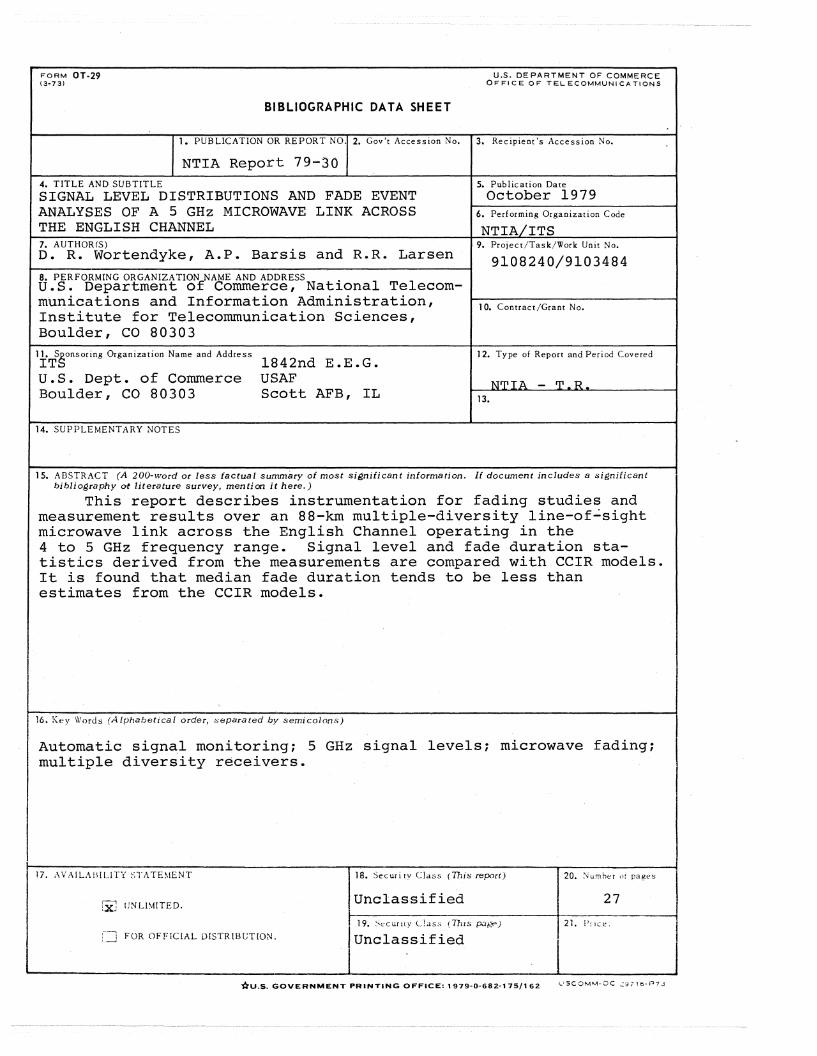
NTIA Report 79-304. TITLE AND SUBTITLE
SIGNAL LEVEL DISTRIBUTIONS AND FADE EVENTANALYSES OF A 5 GHz MICROWAVE LINK ACROSSTHE ENGLISH CHANNEL7. AUTHOR(S)D. R. Wortendyke, A.P. Barsis and R.R. Larsen
8. PERFORMING ORGANIZATION NAME AND ADDRESS •U.S. Department of Commerce, Natlonal Telecom-munications and Information Administration,Institute for Telecommunication Sciences,Boulder, CO 80303
5. Publication Date
October 19796. Performing Organization Code
NTIA/ITS9. Project/Task/Work Unit No.
9108240/9103484
10. Contract/Grant No.
l:i:.TSSonsoring Organization Name and Address
U.S. Dept. of ConunerceBoulder, CO 80303
14. SUPPLEMENTARY NOTES
1842nd E.E.G.USAFScott AFB, IL
12. Type of Report and Period Covered
NTIA - T.R.13.
15. ABSTRACT (A 200-word or less factual summary of most significant information. if document in cludes a significantbibliography at literature survey, mention it h ere,')
This report describes instrumentation for fading studies andmeasurement results over an 88-kmmultiple-diversity line-of~sight
microwave link across the English Channel operating in the4 to 5 GHz frequency range. Signal level and fade duration statistics derived from the measurements are compared with CCIR models.It is found that median fade duration tends to be less thanestimates from the CCIR models.
16. Key Words (AlphabetIcal order, s epera t ed by s etni col ons )
Automaticsign~l monitoring; 5 GHz signal levels; microwave fading;multiple diversity receivers.
17. ;\ VAILABILITY STi\TE~lENT
lxJ UN LIMITED.
:-~=.J FOR OFFiCIAL DISTRIBCTION.
18. Se c ur i tv Class (111is report)
Unclassified!
Unclassified
I
20. Nurn be r of pages
27
21. P~lce.
'ttU.S. GOVERNMENT PR INTING OFFICE: 1979-0-682-175/162 l' 5C OMM· DC ,29716- P7.3