Embed Size (px)
Citation preview

SIGNAL DESIGN FOR MIMO–OFDM SYSTEMS
by
Harry Zhi Bing Chen
M.A.Sc., The University of British Columbia, 2004M.E., University of Science and Technology of China, 2000B.E., Huazhong University of Science and Technology, 1990
A THESIS SUBMITTED IN PARTIAL FULFILLMENT OFTHE REQUIREMENTS FOR THE DEGREE OF
DOCTOR OF PHILOSOPHY
in
THE FACULTY OF GRADUATE STUDIES
(Electrical and Computer Engineering)
THE UNIVERSITY OF BRITISH COLUMBIA
(Vancouver)
January 2010
c© Harry Zhi Bing Chen, 2010

ii
Abstract
Orthogonal frequency division multiplexing (OFDM) combined with multiple–input
multiple–output (MIMO) wireless technology is an attractive air–interface solution for
wireless systems. The time-selective and dispersive nature of the wireless channel, how-
ever, poses challenges for signal design. To address these challenges, this dissertation
investigates several physical layer aspects of signal design for MIMO–OFDM systems.
To improve the information outage rate of certain MIMO systems with low–rank
channel matrices, we propose two novel channel augmentation schemes, namely, the
complex virtual antenna (CVA) and the real virtual antenna (RVA) schemes. For Bell
labs space–time (BLAST) type architectures, both the CVA and the RVA schemes are
more robust to channel correlations than a previously proposed scheme.
For performance enhancement of coded MIMO–OFDM, we consider wrapped space-
frequency coding (WSFC) and coded vertical BLAST (V–BLAST) with adaptive bit
loading (ABL) and optimize both schemes. We show that bit–loaded WSFC and V–
BLAST optimized for coded MIMO–OFDM can achieve error rate performances close
to that of quasi–optimal MIMO–OFDM based on single value decomposition (SVD) of
the channel, while their feedback requirements for loading are low.
To exploit the spatial and frequency diversity in coded MIMO–OFDM systems, we
propose cyclic space–frequency (CSF) filtering, which is applicable to both traditional
MIMO systems with co–located transmit antennas and cooperative diversity systems

Abstract iii
with distributed transmit antennas. We further propose a robust CSF filtering scheme,
which exploits imperfect channel state information at the transmitter (CSIT) and takes
into account the reliability of the CSIT. To further improve robustness, we combine CSF
filtering with space–time block coding (STBC) in the frequency domain. We also propose
a linear prediction method for improving the quality of the CSIT via post–processing.
For these CSF filtering schemes, design criteria are derived, closed–form solutions are
given for certain special cases, and various design methods are provided for the general
case. Simulation results confirm that (robust) CSF filtering is a promising solution for
wireless communication systems.

iv
Contents
Abstract . . . . . . . . . . . . . . . . . . . . . . . . . . . . . . . . . . . . . . . . ii
Contents . . . . . . . . . . . . . . . . . . . . . . . . . . . . . . . . . . . . . . . iv
List of Tables . . . . . . . . . . . . . . . . . . . . . . . . . . . . . . . . . . . . ix
List of Figures . . . . . . . . . . . . . . . . . . . . . . . . . . . . . . . . . . . . x
List of Abbreviations . . . . . . . . . . . . . . . . . . . . . . . . . . . . . . . . xv
Notation . . . . . . . . . . . . . . . . . . . . . . . . . . . . . . . . . . . . . . . xix
Acknowledgments . . . . . . . . . . . . . . . . . . . . . . . . . . . . . . . . . . xxi
1 Introduction . . . . . . . . . . . . . . . . . . . . . . . . . . . . . . . . . . . 1
1.1 MIMO Wireless Communications . . . . . . . . . . . . . . . . . . . . . . 2
1.2 OFDM Modulation . . . . . . . . . . . . . . . . . . . . . . . . . . . . . . 4
1.3 MIMO–OFDM Systems . . . . . . . . . . . . . . . . . . . . . . . . . . . 6
1.4 Thesis Contributions and Organization . . . . . . . . . . . . . . . . . . . 8
2 Preliminaries . . . . . . . . . . . . . . . . . . . . . . . . . . . . . . . . . . . 11
2.1 MIMO Channel Model . . . . . . . . . . . . . . . . . . . . . . . . . . . . 11

Contents v
2.1.1 Signal Envelope . . . . . . . . . . . . . . . . . . . . . . . . . . . . 12
2.1.2 Characteristics of Multipath Fading . . . . . . . . . . . . . . . . . 13
2.1.3 MIMO Channel Parameters . . . . . . . . . . . . . . . . . . . . . 15
2.2 MIMO Techniques . . . . . . . . . . . . . . . . . . . . . . . . . . . . . . 17
2.2.1 Open–Loop Technique I – Layered Space–Time Processing . . . . 18
2.2.2 Open–Loop Technique II – STC . . . . . . . . . . . . . . . . . . . 21
2.2.3 Closed–Loop Technique I – Spatial Multiplexing via SVD . . . . . 25
2.2.4 Closed–Loop Technique II – Combining Precoding with STBC . . 27
2.3 Virtual MIMO Techniques . . . . . . . . . . . . . . . . . . . . . . . . . . 31
2.3.1 Cooperative Diversity . . . . . . . . . . . . . . . . . . . . . . . . . 31
2.3.2 Channel Augmentation . . . . . . . . . . . . . . . . . . . . . . . . 32
2.4 OFDM Basics . . . . . . . . . . . . . . . . . . . . . . . . . . . . . . . . . 34
2.4.1 Orthogonality of Subcarriers . . . . . . . . . . . . . . . . . . . . . 34
2.4.2 Guard Interval . . . . . . . . . . . . . . . . . . . . . . . . . . . . 35
2.4.3 BICM–OFDM . . . . . . . . . . . . . . . . . . . . . . . . . . . . . 36
2.4.4 Adaptive Loading . . . . . . . . . . . . . . . . . . . . . . . . . . . 38
2.5 MIMO–OFDM . . . . . . . . . . . . . . . . . . . . . . . . . . . . . . . . 40
2.5.1 CDD . . . . . . . . . . . . . . . . . . . . . . . . . . . . . . . . . . 40
3 Two Novel Channel Augmentation Schemes for MIMO Systems . . 44
3.1 Introduction . . . . . . . . . . . . . . . . . . . . . . . . . . . . . . . . . . 44
3.2 System Model . . . . . . . . . . . . . . . . . . . . . . . . . . . . . . . . . 46
3.3 Channel Augmentation Schemes . . . . . . . . . . . . . . . . . . . . . . . 47
3.3.1 Rankin, Taylor, and Martin (RTM) Scheme . . . . . . . . . . . . 47
3.3.2 Conjugate Virtual Antenna (CVA) Scheme . . . . . . . . . . . . . 48
3.3.3 Real Virtual Antenna (RVA) Scheme . . . . . . . . . . . . . . . . 49

Contents vi
3.4 Information Outage Rate . . . . . . . . . . . . . . . . . . . . . . . . . . . 50
3.4.1 V–BLAST . . . . . . . . . . . . . . . . . . . . . . . . . . . . . . . 51
3.4.2 D–BLAST . . . . . . . . . . . . . . . . . . . . . . . . . . . . . . . 52
3.5 Numerical Results . . . . . . . . . . . . . . . . . . . . . . . . . . . . . . . 53
3.6 Conclusions . . . . . . . . . . . . . . . . . . . . . . . . . . . . . . . . . . 56
4 On MIMO–OFDM with Coding and Loading . . . . . . . . . . . . . . 58
4.1 Introduction . . . . . . . . . . . . . . . . . . . . . . . . . . . . . . . . . . 58
4.2 System Model . . . . . . . . . . . . . . . . . . . . . . . . . . . . . . . . . 60
4.3 MIMO Processing for Coded MIMO–OFDM . . . . . . . . . . . . . . . . 61
4.3.1 Wrapped Space-Frequency Coding (WSFC) . . . . . . . . . . . . 61
4.3.2 V–BLAST . . . . . . . . . . . . . . . . . . . . . . . . . . . . . . . 63
4.3.3 SVD . . . . . . . . . . . . . . . . . . . . . . . . . . . . . . . . . . 64
4.4 Adaptive Bit-Loading (ABL) Schemes . . . . . . . . . . . . . . . . . . . 65
4.4.1 Full Loading (FL) . . . . . . . . . . . . . . . . . . . . . . . . . . . 65
4.4.2 Grouped Loading (GL) . . . . . . . . . . . . . . . . . . . . . . . . 65
4.4.3 Modification of Loading for V–BLAST . . . . . . . . . . . . . . . 66
4.5 Results and Discussion . . . . . . . . . . . . . . . . . . . . . . . . . . . . 67
4.5.1 Optimization of WSFC and V–BLAST for MIMO–OFDM with
ABL . . . . . . . . . . . . . . . . . . . . . . . . . . . . . . . . . . 68
4.5.2 Performance Comparisons . . . . . . . . . . . . . . . . . . . . . . 69
4.6 Conclusions . . . . . . . . . . . . . . . . . . . . . . . . . . . . . . . . . . 72
5 Cyclic Space–Frequency Filtering for BICM–OFDM Systems . . . . 73
5.1 Introduction . . . . . . . . . . . . . . . . . . . . . . . . . . . . . . . . . 73
5.2 System Model . . . . . . . . . . . . . . . . . . . . . . . . . . . . . . . . . 75
5.2.1 Network Model . . . . . . . . . . . . . . . . . . . . . . . . . . . . 76

Contents vii
5.2.2 Transmitter . . . . . . . . . . . . . . . . . . . . . . . . . . . . . . 76
5.2.3 Channel Model . . . . . . . . . . . . . . . . . . . . . . . . . . . . 79
5.2.4 Receiver Processing . . . . . . . . . . . . . . . . . . . . . . . . . . 80
5.2.5 Extension to OFDMA . . . . . . . . . . . . . . . . . . . . . . . . 81
5.3 CSF Filter Optimization for Known S . . . . . . . . . . . . . . . . . . . 82
5.3.1 Optimization Criterion . . . . . . . . . . . . . . . . . . . . . . . . 83
5.3.2 Upper Bound on Cost Function f(g) . . . . . . . . . . . . . . . . 86
5.3.3 Closed–Form Solution for Special Cases . . . . . . . . . . . . . . . 86
5.3.4 CSF Filter Design for the General Case . . . . . . . . . . . . . . . 88
5.4 CSF Filter Optimization for Unknown S . . . . . . . . . . . . . . . . . . 90
5.4.1 Optimization Problem . . . . . . . . . . . . . . . . . . . . . . . . 92
5.4.2 Upper Bound and Closed–Form Solution for Special Case . . . . . 93
5.4.3 CSF Filter Design for General Case . . . . . . . . . . . . . . . . 94
5.5 Simulation Results . . . . . . . . . . . . . . . . . . . . . . . . . . . . . . 96
5.5.1 Co–located Antennas . . . . . . . . . . . . . . . . . . . . . . . . . 96
5.5.2 Distributed Antennas . . . . . . . . . . . . . . . . . . . . . . . . . 101
5.6 Conclusions . . . . . . . . . . . . . . . . . . . . . . . . . . . . . . . . . . 105
6 Robust Transmit Processing for BICM–OFDM Systems with Imper-
fect CSIT . . . . . . . . . . . . . . . . . . . . . . . . . . . . . . . . . . . . . 107
6.1 Introduction . . . . . . . . . . . . . . . . . . . . . . . . . . . . . . . . . 107
6.2 System Model . . . . . . . . . . . . . . . . . . . . . . . . . . . . . . . . . 109
6.2.1 Channel Model . . . . . . . . . . . . . . . . . . . . . . . . . . . . 110
6.2.2 Transceiver Structure for Robust CSF . . . . . . . . . . . . . . . 110
6.2.3 Transceiver Structure for Robust SFC–CSF . . . . . . . . . . . . 112
6.2.4 Bayesian Statistics for Imperfect CSIT . . . . . . . . . . . . . . . 115

Contents viii
6.3 Optimization of the Robust CSF Filters . . . . . . . . . . . . . . . . . . 118
6.3.1 Optimization Problem . . . . . . . . . . . . . . . . . . . . . . . . 119
6.3.2 Solution for Unstructured G . . . . . . . . . . . . . . . . . . . . . 121
6.4 Design of Robust CSF Filters . . . . . . . . . . . . . . . . . . . . . . . . 123
6.4.1 Special Cases . . . . . . . . . . . . . . . . . . . . . . . . . . . . . 123
6.4.2 Solution of Problem with Additional Constraints . . . . . . . . . 125
6.4.3 Gradient Algorithm (GA) . . . . . . . . . . . . . . . . . . . . . . 127
6.5 Simulation Results . . . . . . . . . . . . . . . . . . . . . . . . . . . . . . 128
6.5.1 Robust CSF Filtering . . . . . . . . . . . . . . . . . . . . . . . . . 129
6.5.2 Robust SFC–CSF Filtering . . . . . . . . . . . . . . . . . . . . . . 132
6.5.3 Linear Prediction (LP) . . . . . . . . . . . . . . . . . . . . . . . 134
6.6 Conclusions . . . . . . . . . . . . . . . . . . . . . . . . . . . . . . . . . . 137
7 Conclusions and Future Work . . . . . . . . . . . . . . . . . . . . . . . . 138
7.1 Research Contributions . . . . . . . . . . . . . . . . . . . . . . . . . . . . 138
7.2 Future Work . . . . . . . . . . . . . . . . . . . . . . . . . . . . . . . . . . 140
A Related Publications . . . . . . . . . . . . . . . . . . . . . . . . . . . . . . 142
Bibliography . . . . . . . . . . . . . . . . . . . . . . . . . . . . . . . . . . . . . 144

ix
List of Tables
5.1 Gradient algorithms (GAs) for calculation of the optimum CSF filters for
known and unknown S, respectively. The elements of the gradient vectors
∂f(g)/∂g∗ and ∂f2,K(gS)/∂g∗S are given in (5.22) and (5.30), respectively.
The adaptation constant µ[i] has to be optimized experimentally. The
termination constant ǫ has a small value (e.g. ǫ = 10−6). i denotes the
iteration. . . . . . . . . . . . . . . . . . . . . . . . . . . . . . . . . . . . . 91

x
List of Figures
2.1 V–BLAST structure. . . . . . . . . . . . . . . . . . . . . . . . . . . . . . 19
2.2 D–BLAST structure. . . . . . . . . . . . . . . . . . . . . . . . . . . . . . 20
2.3 D–BLAST format. . . . . . . . . . . . . . . . . . . . . . . . . . . . . . . 20
2.4 WSTC format. . . . . . . . . . . . . . . . . . . . . . . . . . . . . . . . . 21
2.5 System structure combining beamforming with STBC for a system with
imperfect CSIT. . . . . . . . . . . . . . . . . . . . . . . . . . . . . . . . . 27
2.6 (a) Concept of CP guard interval and (b) OFDM symbol time with CP. . 36
2.7 Block diagram of BICM–OFDM. . . . . . . . . . . . . . . . . . . . . . . 37
2.8 Block diagram of CDD. . . . . . . . . . . . . . . . . . . . . . . . . . . . . 41
3.1 Outage probability vs. outage rate for V–BLAST with MMSE–SIC re-
ceiver and different channel augmentation schemes. ρ = 0.9 and NT =
NV = 4. . . . . . . . . . . . . . . . . . . . . . . . . . . . . . . . . . . . . 54
3.2 Outage rate vs. correlation coefficient ρ for V–BLAST with MMSE–SIC
receiver and different channel augmentation schemes. Pout = 0.01 and
NT = NV = 4. . . . . . . . . . . . . . . . . . . . . . . . . . . . . . . . . . 55

List of Figures xi
3.3 Outage rate vs. number of transmit antennas NT for D–BLAST with
MMSE–SIC receiver and the CVA scheme and OSTBCs. ρ = 0.6, Pout =
0.01. NV = 1 represents the baseline scheme. SNRs of (a) 0 dB, (b) 12
dB, and (c) 24 dB. . . . . . . . . . . . . . . . . . . . . . . . . . . . . . . 57
4.1 Block diagram of the MIMO–OFDM system with adaptive bit loading.
(I)FFT denotes (inverse) fast Fourier transform. . . . . . . . . . . . . . 60
4.2 Example of a WSFC codeword matrix with NT = 3, d = 3, and K = 384.
The indices of the coded symbols are shown in the blocks. . . . . . . . . 62
4.3 SNR required for WSFC to achieve BER = 10−3 vs. interleaving delay d
with R = 2 bits and 4 bits. . . . . . . . . . . . . . . . . . . . . . . . . . . 69
4.4 BER required for V–BLAST with and without ordering vs. extra margin
ηextra . . . . . . . . . . . . . . . . . . . . . . . . . . . . . . . . . . . . . . 70
4.5 BER performance for coded MIMO–OFDM with and without ABL. R =
2 bits, and d = 16 for WSFC. . . . . . . . . . . . . . . . . . . . . . . . . 71
4.6 SNR required to achieve BER = 10−3 for WSFC and V–BLAST with
ordering based MIMO–OFDM with different group sizes G for ABL. R =
2 bits, and d = 16 for WSFC. The center subcarrier and equivalent SNR
methods are used for loading. . . . . . . . . . . . . . . . . . . . . . . . . 72
5.1 Example of a simple two–phase transmission with N = 10 potentially
cooperating relay nodes. NT = 4 relay nodes (S = 1, 3, 9, 10) success-
fully decode the packet received from the source node (S) and forward it
to the destination node (D). . . . . . . . . . . . . . . . . . . . . . . . . . 77
5.2 Block diagram of a) transmitter with NT co–located antennas employing
BICM–OFDM and CSF filtering, and b) transmitter of the nth relay node
employing BICM–OFDM and CSF filtering. . . . . . . . . . . . . . . . . 77
List of Figures xii
5.3 Ratio α , f(g)/f(Gopt) vs. Lg for GA–CSF, EV–CSF, and O–CDD
filters, respectively. NT = 4, ρ = 0.9, and L = 5. . . . . . . . . . . . . . . 98
5.4 BER of BICM–OFDM with GA–CSF filtering, BM–CDD [87], and Alam-
outi’s STBC vs. Eb/N0. OFDM, K = 64, BPSK, NT = 2, and ρL = 0.
GA–CSF filtering: 8 × 8 block interleaver, Lg = 2 for L = 1, Lg = 6 for
L = 5. BM–CDD: 8 × 8 block interleaver and no interleaver. Alamouti’s
STBC: 16 × 8 block interleaver. Convolutional code with (171, 133)8,
R = 1/2, and dfree = 10. . . . . . . . . . . . . . . . . . . . . . . . . . . . 99
5.5 BER of BICM–OFDMA with GA–CSF filtering, O–CDD, BM–CDD [87],
and C–CDD [98] vs. Eb/N0. U = 4, K = 512, 16–QAM, NT = 4, L = 5,
ρL = 0, 32 × 16 block interleaver. Convolutional code with (171, 133)8,
R = 1/2, and dfree = 10. . . . . . . . . . . . . . . . . . . . . . . . . . . . 100
5.6 Minimum coding gain Cmin of GA–CSF filtering for various Lg, upper
bound Cb,k for known S and Lg = 2, and upper bound Cu,k for unknown
S and Lg = 2 vs. N . L = 1, NT = Na = 2, K = 128, 16–QAM, and
16 × 32 block interleaver. . . . . . . . . . . . . . . . . . . . . . . . . . . . 102
5.7 BER of BICM–OFDM with GA–CSF, R–CSF, R–CDD, and C–CDD [86]
filtering when S is unknown vs. Eb/N0. For comparison the BER of GA–
CSF filtering when S is known is also shown. N = 10, L = 1, NT = Na =
2, K = 128, 16–QAM, and 16× 32 block interleaver. Convolutional code
with (171, 133)8, R = 1/2, and dfree = 10. . . . . . . . . . . . . . . . . . . 103

List of Figures xiii
5.8 BER of BICM–OFDM with GA–CSF and C–CDD [86] filtering when S
is unknown vs. Eb/N0. For comparison the BER of GA–CSF filtering
when S is known is also shown. The effects of imperfect synchronization
(IS) and NT = 5 6= Na = 2 are considered. N = 10, L = 1, Na = 2,
K = 128, 16–QAM, and 16 × 32 block interleaver. Convolutional code
with (171, 133)8, R = 1/2, and dfree = 10. . . . . . . . . . . . . . . . . . . 104
5.9 BER at destination node for two–hop transmission with GA–CSF, R–
CSF, and C–CDD [86] filtering when S is unknown vs. Eb/N0. For com-
parison the BER of GA–CSF filtering when S is known is also shown.
Each relay node listens to source node with probability p. N = 10, L = 1,
Na = 2, K = 128, 16–QAM, and 16× 32 block interleaver. Convolutional
code with (171, 133)8, R = 1/2, and dfree = 10. . . . . . . . . . . . . . . . 105
6.1 Block diagram of transceiver for BICM–OFDM with robust CSF. . . . . 111
6.2 Block diagram of transceiver for BICM–OFDM with robust SFC–CSF. . 115
6.3 BER of BICM–OFDM with robust CSF filtering vs. Eb/N0 for Lg = 5.
NT = 3, L = 2, and outdated CSIT. . . . . . . . . . . . . . . . . . . . . . 130
6.4 BER of BICM–OFDM with robust CSF filtering vs. ρ for Lg = 5. Further-
more, results for CSF filters optimized under the assumption of perfect
and statistical CSIT are also shown. NT = 3, L = 2, and outdated CSIT. 131
6.5 BER of BICM–OFDM with robust CSF filtering vs. Eb/N0 for Lg = 1
and Lg = 5. NT = 3, L = 2, and outdated CSIT. . . . . . . . . . . . . . . 132
6.6 BER of BICM–OFDM with robust CSF (Lg = 3) and robust SFC–CSF
(Lg = 2) filtering vs. 1/SQNR. NT = 3, L = 1, ρ = 0.999, and quantized
CSIT. . . . . . . . . . . . . . . . . . . . . . . . . . . . . . . . . . . . . . 133

List of Figures xiv
6.7 BER of BICM–OFDM with robust CSF (Lg = 5) and robust SFC–CSF
(Lg = 2) filtering vs. ρ. NT = 3, L = 2, and outdated CSIT. . . . . . . . 134
6.8 BER of BICM–OFDM with robust CSF filtering vs. Eb/N0. NP = 4,
NT = 3, L = 1, Lg = 3, and outdated CSIT. . . . . . . . . . . . . . . . . 135
6.9 BER of BICM–OFDM with robust CSF filtering vs. ρ. NT = 2, L = 5,
Lg = 6, and outdated CSIT. . . . . . . . . . . . . . . . . . . . . . . . . . 136

xv
List of Abbreviations
3GPP 3rd Generation Partnership Project
4G The Fourth-Generation Mobile Wireless System
ABL Adaptive Bit Loading
ADSL Asymmetric Digital Subscriber Lines
AF Amplify-and-Forward
AWGN Additive White Gaussian Noise
BER Bit–Error–Rate
BICM Bit Interleaved Coded Modulation
BLAST Bell Labs Layered Space–Time
BM Bauch and Malik
BPSK Binary Phase Shift Keying
BWA Broadband Wireless Access
CC Convolutional Code
CCB Chow, Cioffi and Bingham
CDD Cyclic Delay Diversity
CDF Cumulative Distribution Function
CDMA Code Division Multiple Access
CE Consumer Electronics
CIR Channel Impulse Response
List of Abbreviations xvi
CM Channel Model
CP Cyclic Prefix
CSF Cyclic Space–Frequency
CSI Channel State Information
CSIT CSI at the Transmitter
CVA Conjugate Virtual Antenna
DAB Digital Audio Broadcasting
DD Delay Diversity
D–BLAST Diagonal BLAST
DF Decode-and-Forward
DFT Discrete Fourier Transform
DSTC Distributed Space–Time Coding
DSTF Distributed Space–Time Filtering
DVB Digital Video Broadcasting
EV Eigenvector
FCC Federal Communications Commission
FFT Fast Fourier Transform
GA Gradient Algorithm
GL Grouped Loading
IDFT Inverse Discrete Fourier Transform
IEEE Institute of Electrical and Electronic Engineers
IFFT Inverse Fast Fourier Transform
I In-Phase
ICI Inter–Carrier Interference
i.i.d. Independent and Identically Distributed

List of Abbreviations xvii
ISI Inter–Symbol Interference
LOS Line of Sight
LP Linear Prediction
LMMSE Linear Minimum Mean–Squared Error
LSE Least-Square Error
LTE (3GPP) Long Term Evolution
MIMO Multiple-Input Multiple-Output
ML Maximum Likelihood
MMSE Minimum Mean Square Error
MMSE–SIC MMSE Successive Interference Cancellation
MRC Maximum Ratio Combining
NAC Nulling and Cancelling
O–CDD Optimized CDD
OFDM Orthogonal Frequency Division Multiplexing
OFDMA Orthogonal Frequency Division Multiple Access
pdf Probability Density Function
PEP Pairwise Error Probability
PSD Power Spectral Density
PSP Per–Survivor Processing
Q Quadrature
QAM Quadrature Amplitude Modulation
QPSK Quaternary Phase Shift Keying
RF Radio Frequency
RTM Rankin, Taylor, and Martin
RVA Real Virtual Antenna

List of Abbreviations xviii
SC Single Carrier
SFC Space–Frequency Coding
SINR Signal–to–Interference–plus–Noise–Ratio
SIR Signal–to–Interference–Ratio
SISO Single–Input Single–Output
SIMO Single–Input Multiple–Output
SM Spatial Multiplexing
SNR Signal–to–Noise Ratio
SQNR Signal–to–Quantization Noise Ratio
STC Space–Time Coding
STTC Space–Time Trellis Codes
SVD Singular Value Decomposition
UWB Ultra-Wideband
V–BLAST Vertical BLAST
WL Widely Linear
WLAN Wireless Local Area Network
WMAN Wireless Metropolitan Area Network
WSFC Wrapped Space–Frequency Coding
WSTC Wrapped Space–Time Coding
ZP Zero Padded

xix
Notation
Bold upper case and lower case letters denote matrices and vectors, respectively. The
remaining notation and operators used in this thesis are listed below:
(·)∗ Complex conjugate
[·]T Transpose
[·]H Hermitian transpose
det(·) Matrix determinant
diag(x) Diagonal matrix with the elements of vector x on the main diagonal
ℜ· Real part of a complex number
ℑ· Imaginary part of a complex number
E· Expectation
Pr· Probability of some event
λi(·) ith non–zero eigenvalue of a matrix
Q(·) Gaussian Q–function [1]
r(·) Rank of a matrix
tr(·) Trace of a matrix
∗ Convolution operator
⊛ Cyclic convolution operator
⊗ Kronecker product operator
Iη Identity matrix of dimension η × η

Notation xx
0η All–zero matrix of dimension η × η
0η×1 All–zero column vector of length η
|| · || L2 vector norm
⌈x⌉ Smallest integer larger than x
⌈x⌋ Closest integer to x
vec(·) Vectorization of a matrix

xxi
Acknowledgments
I would like to thank my advisor, Professor Robert Schober, for his support and invalu-
able advice during the course of my Ph.D. study. I am much indebted for his patience
and encouragement over the years. Without his support and guidance, this thesis would
not be possible. I also would like to express my gratitude to Professor Lutz Lampe
for many stimulating and helpful discussions and guidance on the work we have done
together.
I would like to thank the other member of my doctoral committee: Professor Vincent
Wong, the University examiners: Professor Jane Wang and Professor Ozgur Yilmaz, and
the External examiner: Professor Gerhard Bauch, for the time and effort in evaluating
my work and providing valuable feedback and suggestions.
Many thanks go to the members of the Communications Theory Group for all the
fruitful discussions, group meetings, and feedback at many points.
Special thanks to my parents and my brothers for all their support during these years.
My deepest gratitude to my wife for her love and patience. All my work is dedicated to
my father Chen Jinhai, who passed away in May 2007.

1
1 Introduction
Information–theoretic studies have shown that multiple–input multiple–output (MIMO)
communication architectures are able to provide extraordinary high spectral efficien-
cies in rich multipath environments, which are simply unattainable using conventional
techniques [2–4]. Meanwhile, orthogonal frequency–division multiplexing (OFDM) is
regarded as an efficient approach to combat the adverse effects of multipath fading.
For improved power and bandwidth efficiency the combination of OFDM and multiple
transmit and receive antennas, often referred to as MIMO–OFDM, has been exten-
sively studied for wireless communication systems. In such a MIMO–OFDM system,
spatial multiplexing, space–time (or space–frequency) coding, adaptive bit loading, and
special signal processing algorithms are usually employed for signal design in order to
approach the MIMO channel capacity. MIMO–OFDM has already been adopted in ma-
jor wireless standards, such as the IEEE 802.11n wireless local areal networks (WLANs)
[5], the IEEE 802.16e wireless metropolitan area networks (WMANs) [6], and the 3rd
Generation Partnership Project (3GPP) long term evolution (LTE) [7]. In the future,
MIMO–OFDM is expected to be employed in more wireless communication systems,
e.g., the fourth-generation (4G) mobile wireless systems.
The remaining sections of this Introduction are organized as follows. In Section
1.1, we briefly review MIMO wireless systems. In Section 1.2, we discuss the OFDM
modulation scheme. In Section 1.3, we introduce MIMO–OFDM systems, and in Section

1. Introduction 2
1.4, we briefly outline the contributions made in this thesis and the thesis organization.
1.1 MIMO Wireless Communications
In a MIMO wireless communication system, multiple antennas are employed at both
the transmitter and the receiver. Data transmissions over the resulting MIMO channels
may be implemented in different ways to obtain a spatial multiplexing gain, a spatial
diversity gain, or both.
Spatial multiplexing schemes yield a throughput increase by transmitting indepen-
dent information streams in parallel through the spatial channels, and the capacity is
limited by the minimum of the number of transmit and the number of receive antennas.
Several schemes have been proposed to exploit the spatial multiplexing gain, such as the
vertical Bell Labs layered space–time (V–BLAST) [8] and the diagonal Bell labs layered
space–time (D–BLAST) [3] schemes.
Diversity gain is achieved by sending the data signal over multiple independent fading
paths in time, frequency, and space and by utilizing appropriate combining techniques
at the receiver. Spatial diversity is particularly attractive as no bandwidth expansion
is required compared to the two other commonly used diversity techniques, time diver-
sity and frequency diversity. Spatial diversity can be further broken down into receive
diversity and transmit diversity. Space–time coding (STC) schemes, such as delay di-
versity (DD) [9], space–time block codes (STBC) [10, 11], and space–time trellis codes
(STTC) [12], are the well–known transmit diversity techniques, which lead to improved
link reliability.
While the aforementioned benefits of spatial diversity or spatial multiplexing are
realizable with an open–loop configuration, where the receiver alone knows the commu-
nication channel, these benefits are further enhanced in a closed–loop MIMO system,

1. Introduction 3
where the transmitter also knows the channel. By exploiting channel state information
(CSI) at the transmitter (CSIT), eigenbeamforming, which converts a MIMO channel
into a bank of scalar channels without crosstalk from one scalar channel to the others,
achieves both a spatial multiplexing gain and a diversity gain. For example, in a wireless
system with four transmit and two receive antennas, CSIT can more than double the
capacity at a signal–noise–ratio (SNR) of 0.5 dB and add 1.5 bps/Hz to the capacity at
an SNR of 5 dB [13]. Therefore, exploiting CSIT is of great practical interests.
However, in practice, it is often not possible to obtain perfect instantaneous CSIT
due to delays in the feedback channel from the receiver to the transmitter, measurement
noise, and quantization noise. In this case, high performance can only be achieved if not
only the imperfect CSIT itself but also the reliability of the CSIT is taken into account
for transmitter design. For flat fading channels, examples for successful exploitation of
imperfect CSIT can be found in e.g. [14–17]. Furthermore, the effect of linear prediction
of CSIT on the performance of beamforming in flat fading channels has been considered
in [18, 19].
MIMO systems require that multiple antennas are spaced from each other at least
one–half of the wavelength of the transmitted signal to obtain low correlation between
the spatial channels. This requirement fundamentally limits the possibility of having
multiple antennas on small communication devices. It has recently been shown that
node cooperation can be used to create a virtual MIMO system [20, 21], where relays
help the source exploit the spatial diversity of a slow fading channel in a distributed
fashion by decode-and-forward (DF) or amplify-and-forward (AF) relaying.
Research related to cooperative communication started with the introduction of the
relay channel in [22]. Important bounds on the capacity of a three–node relay network
for the additive white Gaussian noise (AWGN) channel were provided in [23]. The
concept of user cooperation diversity was introduced in [21], where two users share
1. Introduction 4
their antennas and resources to obtain a diversity gain through distributed transmission.
Various cooperative transmission protocols were proposed in [20], and their performances
were analyzed in terms of outage behavior in [24]. The idea of distributed space–time
coding (DSTC) was introduced in [20] and various DSTC schemes [25–27] have been
investigated since then.
Channel augmentation is another form of virtual MIMO techniques, where virtual
receive antennas are created for performance improvement without requiring the help
of other nodes. Channel augmentation is realized by means of special signal processing
at both the transmitter and the receiver. In [28] the fingers of a RAKE receiver were
exploited to form an augmented channel matrix. A virtual MIMO framework for single–
transmitter single–receiver multipath fading channels was developed in [29] to enable
maximum exploitation of channel diversity at both the transmitter and the receiver. A
smart antenna system using virtual array elements was proposed in [30]. Furthermore,
in [31], the information outage rate of MIMO channels was shown to be potentially
improved by repeatedly transmitting the same signal and combining the received signals
in such a way as to increase the effective rank of the MIMO channel.
1.2 OFDM Modulation
OFDM is a special form of multi–carrier transmission that divides a communication
channel into a number of equally spaced frequency bands, over which a number of lower
rate data signals are transmitted. The OFDM transmission scheme has the following
key advantages.
1. OFDM is an efficient means of combating multipath fading in the wireless en-
vironment. By using the inverse fast Fourier transform (IFFT) and cyclic prefix (CP)
insertion at the transmitter, together with FFT and CP removal at the receiver, OFDM

1. Introduction 5
converts a frequency–selective fading channel into a number of parallel flat fading chan-
nels, thus significantly simplifying the receiver design without the need for a complicated
equalizer, necessary for single–carrier transmission.
2. OFDM can potentially enhance the capacity by adapting the data rate and power
to the subcarrier channel condition. This is achieved by using adaptive bit and power
loading techniques, where signal constellations of different size are transmitted over
subcarriers with different gains.
3. OFDM is robust to narrowband interference. The narrowband interference only
affects a small portion of the subcarriers, and the corrupted symbols can possibly be
recovered by using forward error correction (FEC) coding.
4. OFDM facilitates multiple access by allocating multiple users to different subcar-
riers in a single carrier network. This approach is referred to as orthogonal frequency
division multiple access (OFDMA).
The concept of using parallel data transmission and frequency division multiplexing
can be traced back to the 1950s and the 1960s [32, 33]. However, due to the imple-
mentation complexity of the oscillator and demodulator for each subcarrier required
by frequency division multiplexing, the application of OFDM was limited to military
systems at that time. In 1971, Weinstein and Ebert [34] introduced the idea of using
a Discrete Fourier Transform (DFT) for implementation of the generation and demod-
ulation of OFDM signals, eliminating the requirement for banks of analog subcarrier
oscillators. This presented an opportunity for a simple implementation of OFDM, es-
pecially with the use of FFT. Recent advances in integrated circuit technology have
made the implementation of OFDM cost effective. In the 1980s, OFDM was studied
for high–speed modems and digital mobile communications. Since the 1990s, OFDM
has been commercialized in asymmetric digital subscriber lines (ADSL), digital audio
broadcasting (DAB), digital video broadcasting (DVB–T), and more recently several
1. Introduction 6
wireless communication standards [5–7]. In these systems, the combination of OFDM
and FEC coding is necessary to protect the symbols over the subcarriers experiencing
deep fades, achieving a frequency diversity gain inherent in OFDM.
Conventional multicarrier systems use a fixed signal constellation and power across
all subcarriers, thus the overall error probabilities are dominated by the subcarriers with
the worst performance. To maximize the link capacity or to minimize the overall error
probability of an OFDM system, adaptive loading schemes allocate different constella-
tions and powers across the subcarriers according to the measured SNR. Most loading
algorithms can be classified into two categories: rate–adaptive loading and margin–
adaptive loading. The first type of loading aims at maximizing the overall bit rate
(throughput) given a fixed amount of energy. In the second type of loading, the goal is
to determine the bit and power allocation that requires the least amount of energy with
a fixed number of bits per OFDM symbol. A number of algorithms have been proposed
to solve the discrete loading problem in practice. Examples include the Hughes–Hartogs
algorithm [35], the Chow, Cioffi and Bingham algorithm [36], the Fischer and Huber
algorithm [37], and some fast algorithms proposed in [38–40].
1.3 MIMO–OFDM Systems
Most MIMO schemes were initially proposed for flat fading channels and cannot be
directly applied to frequency–selective channels, which are the most practical channels
for broadband wireless communications. On the other hand, OFDM provides an efficient
approach to combat the adverse effect of multipath spread. A combined MIMO–OFDM
approach can benefit from the advantages of both OFDM and MIMO to enable spatial
multiplexing gains and diversity gains over frequency–selective channels.
Since OFDM results in a number of parallel flat–fading channels, existing MIMO

1. Introduction 7
techniques proposed for single–carrier transmission can be applied to each subcarrier.
Spatial multiplexing is performed by transmitting independent data streams on a sub-
carrier–by–subcarrier basis with the total transmit power split uniformly across anten-
nas and subcarriers. Due to a large number of subcarriers, the computational com-
plexity of spatial multiplexing for MIMO–OFDM could be extremely high. In [41], an
interpolation–based method was introduced to alleviate this problem by taking advan-
tages of the correlation between subcarriers.
Exploiting the presence of the spatial diversity offered by multiple antennas, STC
relies on simultaneous coding across space and time to achieve a diversity gain. OFDM
offers frequency diversity by coding and interleaving across subcarriers and appropriate
decoding algorithms. A straightforward way to realize space–frequency diversity is to
apply existing space–time codes to code across space and frequency (subcarrier) [42, 43].
However, space–frequency coding (SFC), which spreads the symbols across space and
frequency together with bit–interleaved coded modulation (BICM) [44], achieves space
and frequency diversity in a more systematic fashion [45–48].
A particularly simple and efficient form of SFC is cyclic delay diversity (CDD) which
is a straightforward extension of linear DD introduced in [9] for single–carrier trans-
mission to multi–carrier systems. In CDD the same signal is transmitted over different
antennas with different cyclic delays [49, 50]. CDD increases the frequency selectivity of
the channel without increasing the length requirements for the CP. In fact, CDD trans-
forms spatial diversity into additional frequency diversity which can be picked up by an
appropriate FEC coding scheme. In this context, BICM is particularly interesting due
to its simplicity and high performance [51]. In fact, it has been shown that CDD with
BICM can exploit the full spatial and spectral diversity of the channel if the combination
of cyclic delay, interleaver, and free distance of the code is carefully chosen [51].
The detailed literature review relevent to specific prior work will be given in Chap-

1. Introduction 8
ters 3 ∼ 6.
1.4 Thesis Contributions and Organization
This thesis considers several issues regarding the design of MIMO–OFDM systems from
the point of view of signal processing. The goal is to design a high performance MIMO–
OFDM system with affordable computational complexity. The main contributions of
this thesis are as follows.
1. We propose two novel channel augmentation schemes for MIMO systems, which
can achieve a better outage performance than a previously proposed scheme with the
same low computational complexity.
2. We propose several modifications for MIMO–OFDM combined with adaptive
bit-loading (ABL) and FEC coding that improve the frame and bit error rates.
3. We propose cyclic space–frequency (CSF) filtering for BICM–OFDM systems with
multiple co–located or distributed transmit antennas to achieve a spatial and frequency
diversity gain.
4. We propose robust CSF filtering for MIMO–OFDM, which exploits imperfect
CSIT and takes into account the reliability of the CSIT via a Bayesian model.
While the first contribution is related to generic MIMO systems, the remaining con-
tributions are pertinent to MIMO–OFDM systems. In the following, we provide a brief
overview of the remainder of this thesis.
In Chapter 2, we first introduce some background material and important results on
MIMO–OFDM that are relevant to our proposed signal design schemes in Chapters 3–6.
In Chapter 3, we present the proposed channel augmentation schemes for MIMO
systems. Recently, Rankin, Taylor, and Martin (RTM) [31] proposed a simple channel
augmentation scheme for MIMO systems by repeatedly transmitting the same symbols

1. Introduction 9
in several time slots and appropriate combining techniques at the receiver. This scheme
was shown to be able to improve the outage rate of slow fading MIMO channels. Inspired
by [31] we propose two channel augmentation schemes having the same low complexity
as the RTM scheme. In the first scheme, the transmitted symbols are both repeated
and complex conjugated leading to the conjugate virtual antenna (CVA) scheme. In the
second, the transmitted symbols are constrained to be real–valued leading to the real
virtual antenna (RVA) scheme. We show that the RTM, CVA, and RVA schemes can
achieve a higher outage rate than the baseline scheme without augmentation for both
V–BLAST and D–BLAST. The novel RVA and CVA schemes are shown to be more
robust to channel correlation than the RTM scheme.
Chapter 4 deals with MIMO–OFDM combined with ABL and FEC coding. We inves-
tigate “simple” coding schemes and their combination with ABL for MIMO–OFDM. In
particular, we consider wrapped space–frequency coding (WSFC) and coded V–BLAST
with ABL and optimize both schemes to mitigate error propagation inherent in the
detection process. Simulation results show that bit–loaded WSFC and V–BLAST opti-
mized for coded MIMO–OFDM achieve excellent error rate performances, close to that
of quasi–optimal MIMO–OFDM based on singular value decomposition (SVD) of the
channel, while their feedback requirements for loading are low.
In Chapter 5, we introduce CSF filtering for OFDM systems using BICM and multiple
transmit antennas for fading mitigation, and discuss the extension to OFDMA systems.
CSF filtering is a simple form of SFC and may be viewed as a generalization of CDD
where the cyclic delays are replaced by CSF filters. CSF is applicable to both traditional
MIMO systems with co–located transmit antennas and cooperative diversity systems
with DF relaying and distributed transmit antennas. Similar to CDD and in contrast to
other SFC schemes, CSF filtering does not require any changes to the receiver compared
to single–antenna transmission. Based on the asymptotic PEP of the overall system

1. Introduction 10
we derive an optimization criterion for the CSF filters for co–located and distributed
transmit antennas, respectively. We show that the optimum CSF filters are independent
of the interleaver if they do not exceed a certain length. If this length is exceeded, the
adopted interleaver has to be carefully taken into account in the CSF filter design. For
several special cases we derive closed–form solutions for the optimum CSF filters and for
the general case we provide various CSF filter design methods. Our simulation results
show that CSF filtering can achieve significant performance gains over existing CDD
schemes.
Chapter 6 is concerned with robust CSF filtering, which exploits imperfect CSIT and
takes into account the reliability of the CSIT via a Bayesian model. To further improve
robustness, we combine CSF filtering with STBC in the frequency domain and refer to
the resulting scheme as SFC–CSF filtering. We also propose a linear prediction method
for improving the quality of the CSIT via post–processing. Based on an upper bound on
the worst–case pairwise error probability we formulate an optimization problem for the
robust CSF filters which can be solved exactly for certain special cases. For the general
case, we obtain an approximate solution by solving a related problem with additional
constraints. This approximate solution can be further improved with a gradient algo-
rithm for the original problem. Simulation results confirm the excellent performance
of BICM–OFDM with robust CSF and SFC–CSF filtering and the effectiveness of the
proposed CSIT post–processing method.
Finally, Chapter 7 summarizes the contributions of this thesis and outlines areas of
future research.

11
2 Preliminaries
This chapter introduces some relevant background material related to MIMO–OFDM
systems. We present in Section 2.1 MIMO fading channel models that will be considered
for the rest of this thesis. Various MIMO signal processing schemes have been developed
according to the nature of the available CSI at the transmitter and the receiver. We
discuss these MIMO techniques in Section 2.2. In some situations, multiple antennas
are not available, virtual MIMO techniques can be used to achieve a diversity gain
or to improve outage performance. We introduce virtual MIMO techniques in Section
2.3. OFDM is a popular method for transmission over frequency–selective channels.
We present the basic principle of OFDM as well as a related performance enhancement
method, namely, adaptive loading, in Section 2.4. OFDM is often combined with MIMO
to form a so–called MIMO–OFDM architecture for improved power and bandwidth
efficiency. We discuss MIMO–OFDM and focus on the existing SFC schemes in Section
2.5.
2.1 MIMO Channel Model
The key characteristics of the wireless channel are the variations of the channel strength
over time and frequency. These variations are often classified into scales [52, 53]: large
and small. Large scale fading captures path loss and shadowing, which result from sig-

2. Preliminaries 12
nal attenuation with distance and random blockage by large objects, such as hills and
buildings. Small scale fading captures the variation arising from signals of multiple ran-
dom paths adding constructively and destructively. Since signal processing for wireless
communication usually exploits the small scale channel variations, this section focuses
on small scale channel models.
2.1.1 Signal Envelope
Small-scale variation of a channel causes a rapid fluctuation of the received signal enve-
lope. The in-phase (I) and quadrature (Q) components of the received signal are sums of
many independent random variables because of multipath propagation. From the central
limit theorem, both the I and Q components of the channel gain can be approximated
as Gaussian random variables XI and XQ with variance σ2 [52]. The envelope of the
channel response with a non-zero mean resulting from a direct path, Z =√
X2I + X2
Q,
is a Ricean distributed random variable given by [53]
p(z) =z
σ2exp
(
−z2 + s2
2σ2
)
I0
(zs
σ2
)
, for z ≥ 0, (2.1)
where 2σ2 is the average power in the multipath components and s2 is the power of the
direct path component. The function I0(x) is the zeroth order modified Bessel function
of the first kind defined as
I0(x) ,1
2π
π∫
0
ex cos θdθ. (2.2)
The Ricean factor KR is defined as the ratio of the direct path power and the average
multipath power
KR ,s2
2σ2. (2.3)

2. Preliminaries 13
We can write the Ricean distribution in terms of parameter KR as
p(z) =2z(KR + 1)
Ωp
exp
(
−KR − (KR + 1)z2
Ωp
)
I0
(
2z
√
KR(KR + 1)
Ωp
)
, for z ≥ 0, (2.4)
where Ωp = 2σ2 + s2 is the total average power of the direct path and the multipath.
If KR = 0, both XI and XQ have zero means. As a result, a Ricean random variable
becomes a Rayleigh random variable with
p(z) =z
σ2exp(
− z2
2σ2
)
, for z ≥ 0. (2.5)
2.1.2 Characteristics of Multipath Fading
When an ideal impulse is transmitted over a time–varying multipath fading channel,
there will be two effects on the received signal. First, the received signal may appear
as a train of pulses with different delays and magnitudes due to the different lengths
and attenuation factors of different signal paths. Second, the multiple paths are varying
with time because of the random nature of the wireless channel. Thus, the number of
received pulses, the delay between them, and their magnitudes may vary over time. The
impulse response of the channel captures both of these effects, and exhibits spectral and
temporal selectivity.
It is usually convenient to represent the channel in a discrete–time model for digital
signal processing. The commonly used tapped–delay–line model is given by [52]
y[k] =L−1∑
l=0
h[k; l]x[k − l] + n[k], (2.6)
where y[k], x[k], and n[k] are the received signal, the transmitted signal, and the noise
samples at sampling instant k, respectively, and h[k; l] represents the sampled time-

2. Preliminaries 14
varying channel impulse response (CIR) of finite memory L.
Spectral selectivity is caused by the presence of multipath. The channel frequency
response varies with frequency, leading to selectivity. The longer the multipath delays,
the more frequency selective the channel becomes. A measure for this selectivity is the
delay spread, defined as the range of multipath spread in the channel, Tm = τmax − τmin,
where τmax and τmin are the maximum and minimum multipath delays, respectively. The
channel coherence bandwidth Bc is accordingly defined as Bc ≈ 1/Tm [1].
Temporal selectivity, on the other hand, is caused by motion of the transmitter, the
receiver, or the scatterers in the channel. These motions cause a transmitted single tone
to be spread in frequency at the receiver. This phenomenon is also referred to as Doppler
effect. Suppose a receiver is moving at a constant speed v and the arrival angle of plane
waves incident on the receiver is θ, then, the Doppler shift fd is defined as
fd =v cos θ
λ=
vfc cos θ
c, (2.7)
where λ is the wavelength, fc is the signal frequency, and c is the speed of light. The
maximum Doppler frequency shift fD occurs when cos θ = 1, given by fD = vfc/c.
If the multiple paths are widely distributed in angles, it is reasonable to assume that
the arrival angles are uniformly distributed over [0, 2π). With the uniform arrival angle
assumption, the Doppler spectrum is given as [1]
S(f) =1
π√
f 2D − (f − fc)2
, fc − fD ≤ f ≤ fc + fD, (2.8)
The time correlation function of the lth tap can be derived from the Doppler spectrum
as
ρ[m; l] = E
h[k; l]h∗k[k + m; l]
= J0(2πfDm∆t), (2.9)
2. Preliminaries 15
where E· is the mean of its argument, J0(x) is the zeroth order Bessel function of the
first kind, and ∆t is the sampling interval between two signal measurements.
An indicator of the temporal selectivity is the channel coherence time, defined as
the time interval over which the channel remains strongly correlated. Clearly, a slowly
changing channel has a large coherence time. Since the coherence time is a statistically
defined quantity, an approximate relation to the maximum Doppler shift is Tc ≈ 1/fD
[1].
For OFDM systems, we usually assume that the channel is constant for at least one
OFDM symbol processing window, leading to the following simplified channel model [52]
y[k] =L−1∑
l=0
h[l]x[k − l] + n[k], (2.10)
with time–invariant CIR h[l].
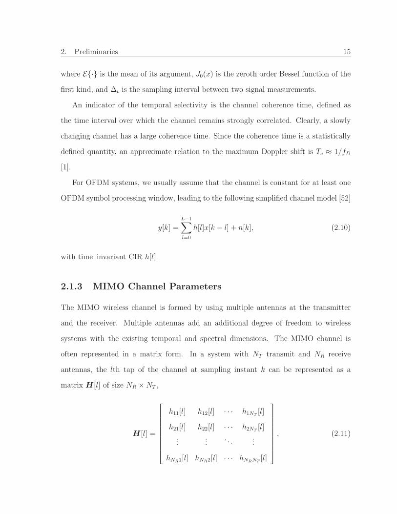
2.1.3 MIMO Channel Parameters
The MIMO wireless channel is formed by using multiple antennas at the transmitter
and the receiver. Multiple antennas add an additional degree of freedom to wireless
systems with the existing temporal and spectral dimensions. The MIMO channel is
often represented in a matrix form. In a system with NT transmit and NR receive
antennas, the lth tap of the channel at sampling instant k can be represented as a
matrix H [l] of size NR × NT ,
H [l] =
h11[l] h12[l] · · · h1NT[l]
h21[l] h22[l] · · · h2NT[l]
......
. . ....
hNR1[l] hNR2[l] · · · hNRNT[l]
, (2.11)

2. Preliminaries 16
where hij[l], 1 ≤ i ≤ NR, 1 ≤ j ≤ NT , is the channel gain from the jth transmit element
to the ith receive element, and can be modeled as a complex Gaussian random process.
These channel gains, however, can be correlated and have different means. The channel
can be decomposed into a fixed part and a variable part as
H [l] = Hm[l] + H [l], (2.12)
where Hm[l] = EH [l] is the channel mean, and H [l] = H [l] − Hm[l] is a zero-mean
complex Gaussian random matrix.
Even at the same time and frequency, the channels resulting from different transmit–
receive antenna pairs could experience different fading, which is related to antenna spac-
ing, the angle of departure of signals, and the angle of arrival of signals. The channel
covariance captures the spatial correlation among all the transmit and receive antennas.
For convenience we collect the CIR coefficients in vector hnr , [hnr[0] hnr[1] . . . hnr[L−
1]]T and define the N = NRNT L dimensional vector h , [hT11 hT
21 . . . hTNT NR
]T contain-
ing all CIR coefficients. The mean and the covariance matrix of h are defined as
mh , Eh (2.13)
Chh , E(h − mh)(h − mh)H. (2.14)
Chh is a positive semidefinite Hermitian matrix and is often assumed to have a separable
Kronecker structure [54, 55], i.e., the transmission and reception fade independently, and
tap correlation can be separated from transmit and receive antenna correlation. In this
case, the channel covariance can now be decomposed as
Chh =1
1 + KR
CNR⊗ CNT
⊗ CL, (2.15)

2. Preliminaries 17
where CNR, CNT
, and CL denote the receive antenna, the transmit antenna, and the
CIR coefficient covariance matrices, respectively, and KR is the Ricean factor.
The channel auto-covariance sequence captures both channel spatial and temporal
correlations. The channel auto-covariance sequence is defined as
Chh[m] , E
h[k]hH [k + m]
, (2.16)
which depends on the time difference m. Here, h[k] is the channel sampled at instant k.
It is often assumed that the temporal correlation is identical for all antenna elements,
thus the spatial and temporal correlation effects are separable, and the channel auto-
covariance becomes
Chh[m] = ρ[m]Chh. (2.17)
2.2 MIMO Techniques
Assuming ideal CSI at the receiver, work on multiple antennas can be classified into
two main classes: open-loop and closed-loop, according to the availability of CSIT. The
former does not require CSI while the latter uses a feedback channel to send CSI acquired
at the receiver back to the transmitter for signal design.
Among the open–loop techniques, layered space–time architectures [3, 56, 57] have
been proposed to achieve high spectral efficiencies while STC [10, 12] has been conceived
mainly for exploiting diversity gains to improve link reliability. Compared with open-
loop techniques, closed-loop techniques have an SNR advantage due to the array gain.
If the transmitter only knows the channel state partially, precoding combined with STC
[14] can achieve high data rates. In the ideal case of perfect CSI available at both sides
of the communication link, the system can be transformed into a set of parallel scalar

2. Preliminaries 18
channels by SVD, followed by waterfilling power allocation to exploit the full channel
capacity [4].
Since initial MIMO research efforts focused on narrowband transmission, we first
consider a system with NT transmit antennas and NR receiver antennas over a flat
fading channel. The NR × 1 vector of received signal samples at the output of the
receive antennas is given by
y = Hx + n, (2.18)
where x is the NT × 1 vector of modulation symbols transmitted with unit energy in
parallel by the NT transmit antennas, H is the normalized NR × NT channel matrix
with Etr[H ] = NT NR, where tr[·] denotes the trace of a matrix, and n is the NR × 1
AWGN vector with each noise element having variance σ2n. The block fading channel is
assumed to be perfectly known at the receiver.
2.2.1 Open–Loop Technique I – Layered Space–Time Process-
ing
In layered space–time architectures, multiple coding streams (layers), each of which cor-
responds to a different transmit antenna, are transmitted simultaneously to exploit the
spatial multiplexing gain of a MIMO system without CSIT. Among the layered space–
time processing schemes are V–BLAST, D–BLAST, and wrapped space–time coding
(WSTC), which will be introduced in this section.
The V–BLAST architecture proposed in [56] uses a vertical layered coding structure
as illustrated in Fig. 2.1. Since optimal maximum–likelihood (ML) detection might
be too complicated, V–BLAST typically relies upon suboptimal low–complexity signal
processing at the receiver. The received signal vector y is first multiplied with a front–end
filter matrix F H , which is obtained according to the zero–forcing (ZF) or the minimum

2. Preliminaries 19
TX Data NT:1
Demux
Code/mod layer 1
Code/mod layer 2
Code/mod layer NT
V-BLAST
signal
processing
RX Data
1
NR
1
2
NT
.
.
..
.
.
Figure 2.1: V–BLAST structure.
mean square error (MMSE) criterion,
v = F Hy. (2.19)
The resulting observable samples are then processed with nulling and cancelation suc-
cessively, where once a layer is successfully decoded, it is subtracted from the received
vector, thus its interference to the remaining layers is canceled. However, if one layer is
decoded incorrectly, this error propagates to all remaining layers. Therefore, the order
of detection of different layers is crucial for the error probability due to the risk of error
propagation. In general, the layers with the lowest error probability should be decoded
first [8, 58–60].
In V–BLAST, each coded layer extends horizontally in the space–time grid and is
placed vertically above each other. Since there is no coding across different transmit
antennas, V–BLAST does not exploit full diversity in the channel, and its performance
is dominated by its worst stream. Therefore, V–BLAST is a suboptimal architecture for
slow–fading channels, and outage occurs whenever one of these streams is in a deep fade
and cannot support the rate of the stream.
Significant improvement of V–BLAST can be achieved by coding across different
antennas. This is the basic idea of D–BLAST [3]. Fig. 2.2 illustrates the high level
system diagram of D–BLAST.
In D–BLAST, multiple codewords are staggered so that each codeword spans multi-

2. Preliminaries 20
TX Data NT:1
Demux
Code/mod layer 1
Code/mod layer 2
Code/mod layer NT
D-BLAST
signal
processing
RX Data
1
NR
1
2
NT
.
.
..
.
.
Figure 2.2: D–BLAST structure.
1
2
3
4
delay
time
1 2 3 4 5 6
codeword 1 codeword 2 codeword 3
ant.
zero symbols
zero symbols
1 2 3 4 5 6
7 8 9 10 11 12
1 2 3 4 5 6
7 8 9 10 11 12 7 8 9 10 11 12
13 14 15 16 17 18 13 14 15 16 17 18 13 14 15 16 17 18
19 20 21 22 23 24 19 20 21 22 23 24 19 20 21 22 23 24
Figure 2.3: D–BLAST format.
ple antennas, but the symbols sent simultaneously by the different antennas belong to
different codewords. Each layer of D–BLAST is striped diagonally across the space–time
grid. Since each diagonal layer constitutes a complete codeword, decoding is performed
layer–by–layer as shown in Fig. 2.3.
From the figure, we observe that in the initialization and termination phase some of
the antennas have to be silent. Therefore, D–BLAST suffers from a rate loss. Never-
theless, as the number of layers increases, D–BLAST approaches the theoretical outage
performance of MIMO systems. In this respect, D–BLAST is an outage-optimal archi-
tecture.
The length of each D–BLAST codeword is the product of the delay and the number
of transmit antennas NT . For a given NT , a large delay is required in order to have a
long codeword, which leads to a smaller rate loss. On the other hand, a small delay
might pose a problem for using trellis codes with large number of states. To solve this
dilemma, WSTC was proposed in [57].

2. Preliminaries 21
1
2
3
4
delay
time
1 5
single codeword
N
ant.
zero symbols
zero symbols
9 13 17
2 6 10 14 18
3 7 11 15 19
4 8 12 16 20
N-1
N-2
N-3
N-4
N-5
N-6
N-7… ...
… ...
… ...
… ...
Figure 2.4: WSTC format.
Unlike D–BLAST, which has several codewords, WSTC uses only a single encoder to
produce a single codeword, which is diagonally interleaved to form a special codeword
matrix as depicted in Fig. 2.4. At the receiver, low–complexity suboptimal decoding is
performed combining decision–feedback equalization and per–survivor processing (PSP),
similar to the nulling and canceling procedure in D–BLAST and V–BLAST. The inter-
ference is canceled by using tentative decisions from the survivor history in the Viterbi
decoder. In WSTC, the interleaver delay can be freely chosen. For the limiting case with
zero delay, WSTC has a vertical structure. For a long codeword, the codeword matrix
can be concatenated to fill the leading and tailing triangles of zeros, which entails no
rate loss.
2.2.2 Open–Loop Technique II – STC
STC achieves a diversity gain by introducing temporal and spatial dependencies into the
signals transmitted from different antennas without increasing the total transmit power
or the transmission bandwidth. The most attractive form of STC is STBC due to its
simplicity, where the information data stream is encoded in blocks.
The simplest example of STC is the DD scheme [9, 61], where the signal transmitted
at sampling instant k from the nth antenna is xn[k] = x[k − ∆n] for 2 ≤ n ≤ NT and

2. Preliminaries 22
x1[k] = x[k], where ∆n denotes the time delay (in symbol periods) on the nth transmit
antenna. Assuming a single receive antenna, the received signal is given by
y[k] =
NT∑
n=1
xn[k] ∗ h[k] + n[k] = x[k] ∗(
h[k] +
NT∑
n=2
h[k − ∆n])
+ n[k], (2.20)
where ∗ denotes the convolution operation, h[k] is the CIR, and n[k] is the AWGN.
From (2.20) it is clear that delay diversity transforms spatial diversity into multipath
diversity that can be exploited through equalization. For flat–fading channels, we can
choose ∆n = (n−1) and achieve full spatial diversity with order NT using ML detection.
We now consider general coherent STBCs. Suppose the information data stream is
divided into groups of Ln source symbols x0, x1, . . . , xLn−1 and these symbols are encoded
as a STBC matrix
B =
b1[0] b2[0] . . . bNT[0]
b1[1] b2[1] . . . bNT[1]
......
. . ....
b1[T − 1] b2[T − 1] . . . bNT[T − 1]
, (2.21)
where bn[t], n = 1, . . . , NT , t = 0, . . . , T − 1, is the encoded symbol transmitted by
antenna nT at time t. The encoded symbols bn[t] are normalized such that the total
energy transmitted by the NT antennas in any symbol interval t is equal to 1. The code
rate R is defined as
R =Ln
T. (2.22)
Assuming coherent detection and perfect channel estimation at the receiver, the PEP
Pe of mistaking an erroneous codeword B1 for the transmitted codeword B0, B0 6= B1

2. Preliminaries 23
is upper bounded by [12]
Pe ≤r(A)∏
i=1
1
λi(A)
(
Es
4N0
)−r(A)
(2.23)
at high SNRs. Here, matrix A is defined as A , EHE, E , B0 − B1, and λi(A)
and r(A) denote the ith non–zero eigenvalue of A and the rank of A, respectively. The
coding gain and diversity gain are defined as
G ,
r(A)∏
i=1
λi(A)
1/r(A)
and d , r(A), (2.24)
respectively. The objective of code design is to make both the diversity gain and the
coding gain as large as possible. At high SNRs, the upper bound in (2.23) is dominated
by the diversity gain d, which determines the asymptotic slope of the bit–error–rate
(BER) curve on the log–log scale. On the other hand, the coding gain specifies the
relative offset of the BER curves of different codes.
In general, the decoding complexity of the ML detection of STBC is exponential in
Ln. In addressing the decoding complexity, Alamouti discovered an ingenious STBC
scheme for transmission with two antennas. In Alamouti’s scheme, the source symbols
are grouped in pairs, where two symbols x0, x1 are simultaneously transmitted in
the first time slot by antennas 1 and 2, respectively. In the next time slot, antenna 1
transmits −x∗1 and antenna 2 transmits x∗
0. This imposes an orthogonal spatial–temporal
structure on the transmitted symbols. Since two symbols are transmitted in two symbol
intervals, the rate of this STBC is R = 1. The STBC matrix can be written as
B =
x0 x1
−x∗1 x∗
0
, (2.25)

2. Preliminaries 24
and the received signals in the two symbol intervals can be collected in the received
vector r , [r[0] r[1]]T given by
r = Bh + n, (2.26)
where h , [h1 h2]T , n , [n[0] n[1]]T , and hν , ν = 1, 2 are the fading gains between
antenna ν and the receive antenna and AWGN, respectively. In particular, the received
signals in the two time slots can be expressed as
r[0] = h1x0 + h2x1 + n[0] and r[1] = −h1x∗1 + h2x
∗0 + n[1], (2.27)
respectively. We define a new received vector y , [r[0] r∗[1]]T such that (2.27) can now
be written as
y = Hx + n, (2.28)
where x , [x0 x1]T , n , [n0 n∗
1]T , and
H ,
h1 h2
h∗2 −h∗
1
. (2.29)
Assuming coherent detection and perfect channel estimation, the ML estimate x for
the information carrying vector x is given by
x = argminx∈X 2
‖y − Hx‖22
, (2.30)
where X 2 is the set of all possible signal vectors for x. Taking advantage of the fact that
HHH = (|h1|2 + |h2|2)I2, where I2 is the 2 × 2 identity matrix, we obtain
y , HHy = (|h1|2 + |h2|2)x + n, (2.31)

2. Preliminaries 25
where n , HHn. It can be easily verified that the elements of n are still i.i.d. Therefore,
the decision rule in (2.30) is equivalent to
x = argminx∈X 2
∥
∥y − (|h1|2 + |h2|2)x∥
∥
2
2
. (2.32)
By using simple linear combining, the joint ML decoding for symbols x0, x1 in
(2.30) is decoupled into two individual decoding problems. The decoding complexity
increases only linearly with the code size L, thus, orthogonal STBCs (OSTBCs) are
very attractive due to their linear decoding complexity.
For real constellations and square matrices B, it was proven in [11] that rate one
(R = 1) codes can exist only for NT = 2, 4, or 8 antennas. However, for complex
constellations, orthogonal designs with R = 1 only exists for the case of NT = 2. Given
the number of transmit antennas NT = 2m − 1, or NT = 2m, where m is a natural
number, the maximum possible rate for complex orthogonal designs was shown to be
R = m+12m
[62].
2.2.3 Closed–Loop Technique I – Spatial Multiplexing via SVD
If the CSI is perfectly known at the transmitter and the receiver, by performing SVD
[4], the channel matrix H can be written as
H = UΣV H , (2.33)
where U and V H are NR×NR and NT×NT unitary matrices, respectively. The entries of
the NR ×NT diagonal matrix Σ, σ1 ≥ σ2 ≥ · · · ≥ σNmin≥ 0 are the sorted non-negative

2. Preliminaries 26
singular values with Nmin = min(NT , NR). Thus, (2.18) can be rewritten as
y = UΣV Hx + n, (2.34)
and the channel can be expressed as
H =
Nmin∑
i=1
σiuivHi , (2.35)
where ui and vi are the columns of U and V , respectively. Let y = UHy , [y1y2 · · · yNR]T ,
x = V Hx , [x1x2 · · · yNT]T , and n = UHn , [n1yn · · · yNR
]T , then the channel in (2.34)
is equivalent to
y = Σx + n, (2.36)
where n still has the same distribution as n. Thus, by applying the weighting matrices
V and UH at the transmitter and the receiver respectively, we obtain equivalent parallel
single–input–single–output (SISO) channels
yi = σixi + ni, 0 ≤ i ≤ Nmin − 1, (2.37)
where yi, xi, and ni are the received symbols, the transmitted symbols, and the AWGN
noise samples over the ith equivalent SISO channel, respectively.
Assuming the components of x are i.i.d., the capacity of the channel [4] is proven to
be
C =
Nmin−1∑
i=0
log
(
1 +P ∗
i σ2i
N0
)
, (2.38)
where N0 is the noise energy per complex symbol time and P ∗i is the power allocated
to the ith SISO channel. This capacity is achieved by allocating power according to the

2. Preliminaries 27
Precoder
F
STBC
Encoder
Channel
HDecoder+
Transmitter
CSIT
B X
N
Y B
Figure 2.5: System structure combining beamforming with STBC for a system withimperfect CSIT.
waterfilling algorithm [4]:
P ∗i =
(
µ − N0
σ2i
)+
, (2.39)
where µ is chosen to meet the total power constraint∑
i P∗i = Ptotal and σi corresponds
to the gain of an eigenmode of the channel.
2.2.4 Closed–Loop Technique II – Combining Precoding with
STBC
While the channel can be measured directly at the receiver with sufficient accuracy, the
transmitter must obtain channel information indirectly, using either channel reciprocity
or feedback, often accompanied by a delay, measurement noise, and quantization errors.
Thus, in practice, the transmitter often obtains imperfect CSIT or partial CSIT, which
leads to performance degradation in a wireless system. However, imperfect CSIT can
be exploited together with the reliability of the CSIT to achieve high performance [14].
One example of successful exploitation of imperfect CSIT is a system configuration
combining a precoder with STBC, where the STBC exploits channel diversity and the
linear precoder exploits the CSIT. The STBC and precoder combination, therefore, is
robust to channel fading and can exploit the available CSIT at the same time. Fig. 2.5
shows the structure of a system combining a linear precoder with STBC [15].
Let the T × NT matrix B be the block codeword in the STBC, then the received

2. Preliminaries 28
signal block is
Y = HFB + N , (2.40)
where F is the linear precoding matrix satisfying the power constraint tr(FF H) = 1
and N is the AWGN matrix. ML detection is performed at the receiver to obtain the
estimate of the codeword
B = argminB∈B
||Y − HFB||2F , (2.41)
where B is the STBC codebook.
The PEP of detecting the transmitted codeword B as another codeword B can be
upper bounded by
P (B → B) ≤ exp
(
−||HF (B − B)||2F4σ2
n
)
. (2.42)
This upper bound can be rewritten as
f(H ,A,F ) = exp(
−ρ
4tr(HFAF HHH)
)
, (2.43)
where ρ = P/σ2n is the SNR and A is defined as 1
P(B − B)(B − B)H with the average
sum transmit power P .
The imperfect CSIT and the true CSI are assumed to be jointly complex Gaussian,
and the pdf of the true channel vector h conditioned on the side information γ is given
by [14]
ph|γ(h|γ) =exp
(
−(h − mh|γ)HC−1
hh|γ(h − mh|γ))
πN det(Chh|γ), (2.44)
where mh|γ = Eh|γ is the conditional mean vector and Chh|γ = E(h − mh|γ)(h −
mh|γ)H |γ is the conditional covariance matrix.

2. Preliminaries 29
The optimal precoder for the case with uncorrelated antennas and the transmitter
knowing the channel means is provided in [14] for OSTBCs. The precoder design for the
more general cases with antenna correlation remains an open question. For the special
case with only transmit antenna correlation and the CSIT in the form of an arbitrary
mean, [15] formulated the precoder optimization problem and provided a solution.
Suppose the channel mean Hm and the transmit correlation matrices CNTare known
to the transmitter. The receive antennas are assumed to be uncorrelated. Averaging
(2.43) over the channel statistics, we obtain the following bound on the average PEP
[15]:
Pe ≤exp(
tr(
HmW−1HHm
)
)
det(W )NRdet(CNT
)NR exp(
tr(
HmW−1HHm
)
)
, (2.45)
where W = ρ4CNT
FAF HCNT+CNT
. Taking the logarithm of this bound and ignoring
the constant terms leads to the following objective function
J(F ) = tr(HmW−1HH) − NR log det(W ) (2.46)
which is convex in the matrix variable W . For OSTBC, A is a scaled identity matrix,
which helps to simplify the optimization problem into the following form:
minF
J(F ) (2.47)
s.t.
W = η0CNTFF HCNT
+ CNT
trF HF = 1,
where η0 = 1/(4µ0ρ).
To solve the optimization problem, define Φ(W ) = C−1NT
WC−1NT
− C−1NT
. Now, the

2. Preliminaries 30
constraints in (2.47) can be rewritten as
tr(Φ) = η0 (2.48a)
Φ 0. (2.48b)
Inequality (2.48b) means that Φ is a positive semi–definite matrix. By using the La-
grangian dual method, the solution for W is obtained as
W =1
2νCNT
(NRINT+ Ψ1/2)CNT
, (2.49)
where Ψ = N2RINT
+4νC−1NT
HHmHmC−1
NT. Here, ν is a parameter to be computed based
on the transmit power constraint. Φ can now be expressed as a function of ν
Φ(ν) =1
2ν(NRINT
+ Ψ1/2) − C−1NT
. (2.50)
The full–mode solution is obtained by solving for ν, assuming Φ is full rank. If the full–
mode solution does not meet the requirement of Φ 0, then the weakest eigenmode
is dropped, forcing its smallest eigenvalue to be zero. This procedure of dropping the
weakest eigenvalues continues until both constraints in (2.48a) and (2.48b) are met
simultaneously. When ν is determined, the optimum solution for F is given by
F =1√η0
UΣ1/2V H , (2.51)
where the matrices U and Σ contain the left singular vectors and the singular values of
Φ, respectively. Here, V can be an arbitrary unitary matrix. From (2.51) the optimal
precoder is not unique and V can be identity matrix for simplicity.
2. Preliminaries 31
2.3 Virtual MIMO Techniques
In the previous section, we have discussed various processing techniques for multiple
antennas. However, in applications such as wireless sensor network and ad hoc network,
implementation of multiple antennas is not always possible due to space limitation or
cost consideration. Virtual MIMO techniques provide us with an alternative means to
achieve a diversity gain or to improve the outage performance.
2.3.1 Cooperative Diversity
The basic idea of cooperative diversity is to allow a collection of nodes to share their
antennas to emulate a virtual antenna array and exploit spatial diversity in wireless
fading channels. In a cooperative network, the source node transmits data symbols to
the destination nodes with the help of relays. A diversity order equal to the number of
cooperative nodes can be achieved.
Various cooperative transmission protocols have been proposed [20, 24]. The two–
phase protocol is the most popular one, where in the first phase, the source node broad-
casts the information to the relay nodes. Then, in the second phase, the relay nodes ei-
ther decode–and–forward (DF) or amplify–and–forward (AF) the received signals to the
destination. At the destination, the received signals are combined to obtain a diversity
gain via certain signal processing techniques. For example, the distributed space–time
coding (DSTC) [20, 63, 64] and distributed space–time filtering (DSTF) [65] schemes
employ the two–phase protocol, and these codes have to be applied at the transmitters.
The relay nodes can be active or non–active depending on whether they participate
in the cooperation or not. Furthermore, depending on the level of cooperation between
the relay nodes, two different approaches can be distinguished. In centralized schemes,
the cooperative nodes know their partners, and numerous existing STC schemes for

2. Preliminaries 32
co–located antennas can be directly applied. In decentralized schemes, the cooperating
nodes are not required to know their partners. Thus, decentralized schemes may be
more flexible and practical, especially in application such as wireless sensor networks
where sensors decide independently about their own actions.
2.3.2 Channel Augmentation
Channel augmentation is another class of virtual MIMO techniques, where virtual anten-
nas are created to increase the effective rank of the channel matrix by means of special
signal processing methods. Channel augmentation can be employed to improve the out-
age performance of a wireless system. For instance, in a communication link, where the
number of transmit antennas exceeds the number of receive antennas, i.e. NR < NT ,
layered space–time architectures such as V–BLAST cannot be applied straightforwardly
since these schemes typically require NT ≤ NR. In this case, an augmented MIMO
channel can be created to obtain more virtual receive antennas than the original channel
has.
In the recently proposed RTM scheme [31], the information outage rate is improved
by simple signal processing of independently faded received signals at the receiver. Sup-
pose a standard uncorrelated MIMO Rayleigh fading channel model with received vector
y modeled as
y = Hx + n, (2.52)
where x is the transmitted data with maximum power P = ExHx, H is the NR ×NT
channel matrix, and n is the noise vector. H and n are independent and both have i.i.d.
elements taken from a complex zero–mean Gaussian distribution with unit variance. The
channel is assumed to be known only at the receiver. At the transmitter, the same data
are sent repeatedly in several time slots, which are assumed to fade independently. For

2. Preliminaries 33
instance, if the data are transmitted in two time slots, the received signals are given by
y1 = H1x + n1, (2.53)
y2 = H2x + n2, (2.54)
where Hν and nν , ν = 1, 2, are the channel matrix and the noise vector in time slot 1
and 2, respectively, and they all mutually independent. At the receiver, to increase the
effective number of receive antennas, the signals received in two time slots are stacked
on top each other to form
z =
y1
y2
=
H1
H2
+
n1
n2
= Gx + v (2.55)
where G has size 2NT × NR and the SNR is still the same as in (2.52). Thus, if
NT ≤ NR/2, the channel rank has been doubled. However, the ergodic capacity is not
improved since the data have been transmitted twice. In fact, the ergodic capacity is
even slightly reduced [31].
The information rate of the augmented channel G, which is known only at the
receiver, is given by
I =1
NV
log2
(
det(
I +P
NT
GGH)
)
, (2.56)
where NV is the number of slots for repeating the same signals. The virtual antenna tech-
nique increases the size and rank of the augmented channel matrix with a corresponding
decrease in data rate. Simulation results show that the improvement in outage rate is
more evident at low outage probabilities (≤ 10−2) than at higher outage probabilities
(≥ 10−1).
Inspired by the RTM scheme, we have proposed two novel channel augmentation

2. Preliminaries 34
schemes, which can achieve a higher outage rate than the RTM scheme with the same
low complexity. We will introduce both schemes in detail in Chapter 3.
2.4 OFDM Basics
The principle of OFDM is to divide a high rate data stream into a number of lower rate
streams that are transmitted simultaneously over a number of channels (subcarriers)
that experience flat fading. These subcarriers are chosen to be orthogonal to each other
so that no guard bands are required. The resulting channel is a sum of orthogonal
subchannels. OFDM is thus capable of achieving a high spectral efficiency, while at
the same time being able to combat multipath fading. Furthermore, a CP is inserted
in every OFDM symbol to eliminate inter–symbol interference (ISI) and inter–carrier
interference (ICI).
2.4.1 Orthogonality of Subcarriers
In an OFDM system, the frequency spacing between adjacent subcarriers is f =
1/(KT ), where the number of the subcarriers is K and the overall symbol rate is 1/T .
With this frequency spacing, the subchannels can maintain orthogonality, although the
subchannels overlap. Therefore, ideally, there is no intersymbol and intercarrier inter-
ference in OFDM systems.
The discrete–time representation of the baseband transmitted signals for one OFDM
symbol period can be expressed as
s[n] =1√K
K−1∑
k=0
a[k]ej2πkn/K , 0 ≤ n ≤ K − 1, (2.57)
where a[k] is the transmitted data symbol over the kth subcarrier. Obviously, the com-

2. Preliminaries 35
plexity of the modulation/demodulation increases with increasing the number of sub-
carriers. However, instead of carrying out the modulation/demodulation on a subcarrier
by subcarrier basis, all OFDM subcarriers are modulated and demodulated in a single
IFFT/FFT step efficiently. For example, using the radix-2 algorithm, a K-point IFFT
requires only (K/2) log2 K complex multiplications. The number of complex multiplica-
tion in the IFFT can be further reduced by using a radix-4 algorithm [66].
At the receiver, a spectral decomposition of the received time domain samples is
performed employing a K-point FFT, and the recovered data symbols are restored in
serial order and demultiplexed.
2.4.2 Guard Interval
If the delay spread of a frequency–selective fading channel is relatively large compared
to the sampling interval, ISI will inevitably occur. To eliminate this undesirable effect,
a guard interval is introduced for each OFDM symbol. The guard time is chosen larger
than the expected delay spread so that no OFDM symbol is interfered by its previous
symbol.
Typically, OFDM systems employ a CP guard internal Tg to protect against ISI as
well as maintaining the orthogonality among subcarriers. The CP is formed by padding
the start of the OFDM symbol using a copy of some fraction of the samples from the
end of the symbol as shown in Fig. 2.6. This ensures that delayed replicas of the OFDM
symbol always have an integer number of cycles within the FFT intervals, as long as the
delay is smaller than the guard time. Therefore, multipath signals with delays smaller
than the guard time do not cause ISI. At the receiver, the prefix samples are discarded,
and the remainder of the samples are converted back into the frequency domain using
the FFT. In this way, the CP transforms linear convolution to cyclic convolution in the

2. Preliminaries 36
TgT
CP
CP T
(a) (b)
Figure 2.6: (a) Concept of CP guard interval and (b) OFDM symbol time with CP.
time domain, which is converted to a simple multiplication in the frequency domain by
the FFT at the receiver. In the IEEE 802.16e standard [6], the length of CP is chosen
between 1/32 to 1/4 of an OFDM symbol interval.
Some systems have adopted zero–padding (ZP) instead of CP. In ZP, the end of
OFDM symbols are postfixed with a number of “0” guard samples. The transmitter
keeps silent during ZP interval and thus does not consume energy. Another benefit of
ZP is that the spectrum of the ZP signal does not have “spikes”, which normally appear
in an OFDM system with CP due to its periodic nature. The second benefit is especially
favored by some systems with power spectrum density (PSD) limits, e.g., the ultra–
wideband (UWB) system. However, the use of ZP introduces additional complexity of
signal processing at the receiver side [67]. Currently most systems employ CP as the
guard interval, thus we consider only CP guards in this thesis.
2.4.3 BICM–OFDM
It has been shown that code diversity can be improved by bit–wise interleaving [68].
Caire et al. presented the theory behind BICM in [57]. Their work provided tools to
evaluate the performance of BICM with tight bounds and design guidelines. BICM can
be combined with OFDM, where coding and modulation are separated by a bit-level
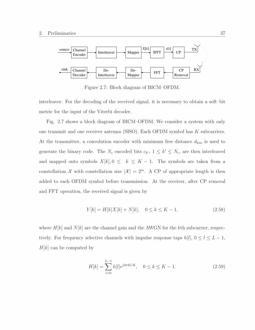
2. Preliminaries 37
Channel
EncoderInterleaver Mapper IFFT CP
Channel
Decoder
De-
Interleaver
De-
MapperFFT
CP
Removal
source
sink
TX
RX
X[k] x[t]
Figure 2.7: Block diagram of BICM–OFDM.
interleaver. For the decoding of the received signal, it is necessary to obtain a soft–bit
metric for the input of the Viterbi decoder.
Fig. 2.7 shows a block diagram of BICM–OFDM. We consider a system with only
one transmit and one receiver antenna (SISO). Each OFDM symbol has K subcarriers.
At the transmitter, a convolution encoder with minimum free distance dfree is used to
generate the binary code. The Nc encoded bits ck′ , 1 ≤ k′ ≤ Nc, are then interleaved
and mapped onto symbols X[k], 0 ≤ k ≤ K − 1. The symbols are taken from a
constellation X with constellation size |X | = 2m. A CP of appropriate length is then
added to each OFDM symbol before transmission. At the receiver, after CP removal
and FFT operation, the received signal is given by
Y [k] = H[k]X[k] + N [k], 0 ≤ k ≤ K − 1, (2.58)
where H[k] and N [k] are the channel gain and the AWGN for the kth subcarrier, respec-
tively. For frequency selective channels with impulse response taps h[l], 0 ≤ l ≤ L − 1,
H[k] can be computed by
H[k] =L−1∑
l=0
h[l]ej2πkl/K , 0 ≤ k ≤ K − 1. (2.59)

2. Preliminaries 38
Based on the received signal, the demapper computes the metric of each coded bit [44, 48]
λi(Y [k], ck′) = minX∈X i
ck′
∣
∣Y [k] − H[k]|2X∣
∣
2
, (2.60)
where X ib denotes the subset of all symbols X ∈ X whose label has the value b ∈ 0, 1
in position i. The metrics are de–interleaved and then sent to a Viterbi decoder. It was
shown in [69] that for an L–tap frequency selective channel, BICM–OFDM can achieve
a diversity order of min(dfree, L) in a SISO system.
2.4.4 Adaptive Loading
When CSIT is available, the transmit power and the bits to be transmitted for each
subcarrier can be adapted according to the CSIT in order to increase data rate or
decrease transmit power consumption. The scheme employed to adaptively allocate
transmit power and bits for each subcarrier, known as adaptive loading, is an important
aspect of the design of an OFDM system over ADSL, and has recently been extended
to wireless OFDM systems. Different strategies can be applied for adaptive loading
[35–37, 70].
It is well known that the waterfilling approach is the capacity–achieving power alloca-
tion algorithm for a spectrally shaped channel [71]. However, the waterfilling algorithm
assumes infinite granularity in constellation size, which is not realizable in practical
communication systems. One finite–granularity loading algorithm, known as Hughes–
Hartogs algorithm [72], mimics the waterfilling approach and yields a near optimal so-
lution by using an incremental strategy. The Hughes–Hartogs algorithm creates a table
of incremental energy required to transmit one additional bit on each of the subcarriers.
Then, at each step, one more bit is added to the subcarrier that requires the least in-
cremental energy, until all bits are assigned or the total power is exceeded depending on

2. Preliminaries 39
the predefined criterion. The extensive sorting needed renders this algorithm impractical
for an OFDM system with a large number of subcarriers. The more efficient algorithms
proposed by Li et al. [70] and Piazzo [40] also use incremental strategy.
One of the solutions that omit the extensive sorting in the Hughes–Hartogs algo-
rithm is the capacity–based strategy in [36], which approximates the channel capacity
of the subcarriers. Let P [k] and σ2n[k] be the transmit power and the noise variance on
subcarrier k, respectively. Then, the rate r[k] for this subcarrier is given by
r[k] = log2
(
1 +P [k]
σ2n[k] · Γγ
)
, (2.61)
where Γ is a fixed bias and γ is a parameter iteratively decided such that the sum rate
over all subcarrier,∑
k r[k], equals the target rate Rtotal. r[k] has to be rounded to the
nearest integer for bit allocation in such a way that the overall quantization error is
minimal. The total transmit power Ptotal is then distributed among the subcarriers such
that the error performances of all subcarriers are identical and∑
k P [k] = Ptotal.
The problem with the capacity–based strategy is that the power and bit allocation
which approximates the capacity is not necessarily the optimum solution for a system
with a specific coding and modulation scheme. Bits and power can also be allocated
using closed–form expression for the probability of error, given the SNR. For instance,
the probability of error for uncoded QAM on subcarrier k is given by [1]
P (Mk, γk) = 4
(
1 − 1√Mk
)
Q
(
3γk
Mk − 1
)
(
1 −(
1 − 1√Mk
)
Q
(
3γk
Mk − 1
)
)
, (2.62)
where Mk and γk are the constellation size and the average symbol energy, respectively.

2. Preliminaries 40
Q(·) is the Q-function defined as
Q(x) ,1
2π
∞∫
x
e−t2/2dt. (2.63)
Subject to a total rate and power constraint, Fischer and Huber [37] distribute the bits
and power to minimize the error probability on each subcarrier. log2(Mk) gives a non–
integer number of bits. After simplifying approximations, Mk can be determined and
rounded to the nearest integer.
2.5 MIMO–OFDM
The main motivation behind using MIMO–OFDM is the fact that OFDM modulation
turns a frequency–selective MIMO channel into a set of parallel flat MIMO channels.
This greatly simplifies the multi–channel equalization at the receiver as for each sub-
carrier only a constant matrix has to be inverted. While spatial multiplexing increases
spectral efficiency, SFC is used to improve link reliability through a diversity gain. SFC
spreads the symbols across space and frequency to exploit space and frequency diversity
in a systematic way. In this section, we will introduce CDD, a particular simple and
efficient form of SFC.
2.5.1 CDD
The block diagram of CDD is depicted in Fig. 2.8. The information bits are encoded
by a forward error correction (FEC) encoder, and are then interleaved and mapped on
quadrature amplitude modulation (QAM) or phase-shift keying (PSK) symbols, which
are assigned to the K subcarriers of an OFDM symbol. A K-point IFFT converts these
symbols from the frequency domain into the time domain. The time domain symbols

2. Preliminaries 41
Channel
EncoderInterleaver Mapper IFFT
CP
Channel
Decoder
De-
Interleaver
De-
MapperFFT
CP
Removal
source
sink RX
X[k]
x[3]~ x[2]~ x[1]~ x[0]~
2
NT
x[3]~x[2]~ x[1]~ x[0]~
CP
CPTX
TX
TX
x[2]~x[1]~ x[0]~ x[3]~
.
.
.
Figure 2.8: Block diagram of CDD.
are denoted as x[k], 0 ≤ k ≤ K−1. Before inserting the CP as guard interval, the time–
domain OFDM symbol is shifted cyclically by ∆n, 1 ≤ n ≤ NT , for transmit antenna
element n. This yields the antenna specific signals:
xn[k] =1√K
x[(k − ∆n)mod K], 0 ≤ k ≤ K − 1, 1 ≤ n ≤ NT . (2.64)
We can simply set the cyclic shift for the first antenna to ∆1 = 0. In contrast to the
cyclic shift ∆n in the case of CDD, conventional DD simply shifts the original data
signals in time domain by antenna specific delays.
For simplicity, we consider a single receive antenna here. The CIR from transmitter
n to the receive antenna is given by
qn[k] =L−1∑
l=0
hn[l]δ[k − l], (2.65)
where the length of the channel is L and hn[l] is the channel gain of the lth tap for
transmit antenna n. We assume that the channel remains constant during one OFDM
symbol interval.
At the receiver, the CP is first removed before FFT is performed. The resulting

2. Preliminaries 42
signal can be expressed by
R[k] = Heq[k]X[k] + N [k], 0 ≤ k ≤ K − 1, (2.66)
where N [k] is an AWGN sample and the channel coefficient Heq[k] is given by
Heq[k] =
NT∑
n=1
L−1∑
l=0
hn[l]e−j2πk(l−∆n)/K . (2.67)
Eq. (2.67) shows that CDD transforms the multiple input channel into an equivalent
single input channel Heq[k] with increased frequency selectivity. The spatial diversity has
been transformed into frequency diversity, which can be picked up by FEC coding. For
the commonly used convolutional code (CC), the minimum free distance dfree determines
the maximum diversity level, where ideally successive bits experience independent fading.
For this purpose, BICM and CCs with a large dfree are favored in order to exploit
maximum frequency diversity.
Selection of the cyclic delay is an important issue that affects the performance of
CDD. The cyclic delay should be chosen such that an FEC decoder can exploit the
full spatial diversity inherent in the channel. To preserve the maximum diversity, the
equivalent channel taps in (2.67) should not contain sums of taps at different delays,
therefore, the cyclic delays should satisfy
∆n ≥ ∆n−1 + L, 2 ≤ n ≤ NT . (2.68)
A safe choice for the cyclic delay is [51]
∆n =(n − 1)K
NT
, 1 ≤ n ≤ NT , (2.69)
2. Preliminaries 43
which yields the largest possible delay difference and low correlation between adjacent
subcarriers.
Compared with OSTBC, CDD has the following major advantages :
1. CDD enjoys low complexity at both the transmitter and receiver. For OSTBC,
an extra IFFT at each transmit antenna and a diversity combiner at the receiver are
required. CDD uses only one IFFT at the transmitter independent of the number of
transmit antennas, and there is no additional processing apart from channel estimation
at the receiver.
2. CDD provides a very flexible space–frequency coding approach for any number
of transmit antennas. The number of transmit antennas can even be changed without
changing the codes used and the receiver structure. Thus, CDD can be easily incor-
porated into existing communication systems. For OSTBC, the number of transmit
antennas can not be easily changed once it is determined.
3. There is no rate loss for CDD compared to a single transmit antenna OFDM.
In contrast, OSTBCs suffer from a rate loss in a system using more than two transmit
antennas, cf. Section 2.2.2.
The performance of CDD can be improved by its generalized version, generalized
CDD (GCDD) [73], or CSF filtering [74], which is one of the main contributions of this
thesis. We will discuss CSF filtering in detail in Chapters 5 and 6.

44
3 Two Novel Channel
Augmentation Schemes for MIMO
Systems 1
3.1 Introduction
In this chapter, we introduce the proposed two novel channel augmentation schemes
for MIMO systems. Channel augmentation schemes belong to a class of virtual MIMO
techniques, where special signal processing methods are applied at the transmitter and
the receiver to create virtual antennas, leading to improved outage performance.
Generally, if the number of transmit antennas significantly exceeds the number of
receive antennas, STC [12] is usually preferred to BLAST–type processing. However,
recently, Rankin, Taylor, and Martin (RTM) [31] have shown that the information outage
rate of MIMO channels can be potentially improved by repeatedly transmitting the same
BLAST–type signal. This is especially true for the case where the number of transmit
antennas is larger than the number of receive antennas. In fact, stacking the received
signal vectors corresponding to the same transmitted symbols results in an augmented
1The material in this chapter was presented in part at IEEE Wireless Communications and Net-
working Conference, Hong Kong, China, March 2007.

3. Two Novel Channel Augmentation Schemes for MIMO Systems 45
MIMO channel with an increased number of virtual receive antennas. This also facilitates
the application of suboptimum processing techniques typically used in BLAST receivers,
cf. Section 2.2.1. The concept of creating virtual receive antennas is not new and has
been shown to be an effective technique for performance improvement in other contexts
before, cf. [29, 75].
In this chapter, we introduce two novel channel augmentation techniques and make
the following contributions.
• The first novel scheme is similar to the RTM technique. However, instead of sim-
ply repeating the transmitted symbols, the symbols are also complex conjugated
leading to the conjugate virtual antenna (CVA) scheme. The CVA scheme has
the same complexity as the RTM scheme but yields a better performance if the
channels seen by the repeated symbols are correlated.
• The second novel scheme restricts the transmitted symbols to be real–valued. By
processing both the real and the imaginary parts of the received signal the number
of receive antennas is essentially doubled. We refer to this approach as real virtual
antenna (RVA) scheme. We will also investigate the relation of the RVA scheme
to so–called widely linear (WL) processing [76, 77].
• While [31] only considered the information outage rate for optimum transmitter
and receiver processing, we investigate the impact of channel augmentation on the
information outage rates of various optimum and suboptimum transmitter and
receiver structures. In particular, we consider V–BLAST and D–BLAST with
linear minimum mean–squared error (LMMSE) and MMSE successive interference
cancellation (MMSE–SIC) receivers.
• Our simulation results confirm that channel augmentation is an efficient approach

3. Two Novel Channel Augmentation Schemes for MIMO Systems 46
to increase the information outage rate for both optimum and suboptimum trans-
mitter/receiver processing and show that the CVA and the RVA schemes achieve
a better performance than the RTM scheme in correlated fading.
The remainder of this chapter is organized as follows. In Section 3.2, the considered
system model is introduced. In Section 3.3, the RTM scheme is briefly reviewed and the
two proposed channel augmentation schemes are presented. The outage performance
of all three schemes is discussed for different transmitter and receiver structures in
Section 3.4. Simulation results are presented in Section 3.5, and some conclusions are
drawn in Section 3.6.
3.2 System Model
We consider a coded MIMO system with NT transmit antennas and NR receive antennas.
In the kth coding frame the received NR × 1 vectors yk can be expressed as
yk = Hkxk + nk, (3.1)
where the NT × 1 vectors xk and nk contain the transmitted data symbols and rota-
tionally symmetric i.i.d. AWGN samples with variance σ2n, respectively.
The channel matrix Hk has size NR × NT , where the (m,n)th element hmn[k] rep-
resents the path gain between the nth transmit antenna and the mth receive antenna.
We assume that Hk does not change during a coding frame (quasi–static channel) and
that the path gains hmn[k] are spatially uncorrelated and complex Gaussian distributed
with variance σ2h , E|hmn[k]|2 = 1. Furthermore, the path gains corresponding to dif-
ferent coding frames may be correlated. Since different coding frames may correspond
to different frequencies or different time slots or both, we use here a generic exponen-

3. Two Novel Channel Augmentation Schemes for MIMO Systems 47
tial correlation model, i.e., Ehmn[k + κ]h∗mn[k] = ρ|κ|, where 0 ≤ ρ < 1 denotes the
correlation coefficient. We note that in [31] only the case of ρ = 0 was considered.
The power of the transmitted symbol vector is constrained to ExHk xk = P . Fur-
thermore, since we consider the scenario in which the instantaneous CSI is only available
to the receiver but not to the transmitter, the total power is equally distributed over all
transmit antennas.
In V–BLAST the NT elements of all xk corresponding to the same coding frame are
separately encoded. In contrast, in D–BLAST all elements of xk are jointly encoded, cf.
Section 2.2.1. In this chapter, we will use the information outage rate as a performance
measure for comparing different channel augmentation schemes. Furthermore, since we
are primarily interested in an information theoretical comparison, we assume that the
elements of xk are i.i.d. real or complex Gaussian distributed.
3.3 Channel Augmentation Schemes
We first briefly review the RTM scheme before we present two novel channel augmenta-
tion schemes, which have the same low computational complexity.
3.3.1 Rankin, Taylor, and Martin (RTM) Scheme
In the RTM scheme [31], also cf. Section 2.2.4, the same complex Gaussian symbol vector
x is transmitted in Kf coding frames to create NV = NRKf virtual receive antennas,
i.e., xk = x, 1 ≤ k ≤ Kf . By stacking the related received vectors yk, 1 ≤ k ≤ Kf , we
obtain
y = Gx + n, (3.2)

3. Two Novel Channel Augmentation Schemes for MIMO Systems 48
where
y , [yT1 yT
2 . . . yTKf
]T , (3.3)
n , [nT1 nT
2 . . . nTKf
]T , (3.4)
G , [HT1 HT
2 . . . HTKf
]T . (3.5)
Eqs. (3.2) and (3.5) show that the RTM scheme creates an augmented NV ×NT channel
matrix G corresponding to NV virtual receive antennas at the expense of a Kf–fold
decrease in data rate. It was shown in [31] that for many practically relevant cases, the
increased rank of the channel matrix outweighs the decrease in data rate as far as the
information outage rate is concerned.
3.3.2 Conjugate Virtual Antenna (CVA) Scheme
The CVA scheme is similar to the RTM scheme. However, instead of simply repeating
the same signal vector Kf times, we also allow complex conjugation, i.e., x2k−1 = x,
1 ≤ k ≤ Kf/2, and x2k = x∗, 1 ≤ k ≤ Kf/2, where Kf is assumed to be even. In
order to get a simple equivalent channel model, the received vectors corresponding to
the complex conjugated transmitted vectors are complex conjugated at the receiver.
Therefore, the resulting augmented channel model is still given by (3.2). However, now
the definitions
y , [yT1 yH
2 yT3 . . . yH
Kf]T , (3.6)
n , [nT1 nH
2 nT3 . . . nH
Kf]T , (3.7)
G , [HT1 HH
2 HT3 . . . HH
Kf]T (3.8)
3. Two Novel Channel Augmentation Schemes for MIMO Systems 49
are valid. Since the elements of nk, 1 ≤ k ≤ Kf , are i.i.d. rotationally symmetric
complex Gaussian random variables, the noise vectors n in (3.5) and (3.8) have the
same statistical properties. Similarly, if the channel matrices Hk in different coding
frames are uncorrelated, the augmented channel matrices G in (3.5) and (3.8) have the
same statistical properties and the RTM and CVA schemes are equivalent and result in
the same information outage rate. However, when the channel matrices Hk, 1 ≤ k ≤ Kf ,
are correlated, i.e., ρ > 0, the CVA scheme is superior as will be shown in Section 3.5.
3.3.3 Real Virtual Antenna (RVA) Scheme
In the RVA scheme, the transmit symbol vector is constrained to have real–valued entries.
To create NV = KfNR virtual antennas, we transmit the real–valued vector xR Kf/2
times, where Kf is assumed to be even. Since compared to the RTM and the CVA
schemes only half of the number of time/frequency slots are required, we assume that
only odd time/frequency slots k are used for transmission to minimize the correlation
of neighboring slots. The even slots can then be used for transmission of independent
data. At the receiver, we stack the real parts and the imaginary parts of the received
vectors y2k−1, 1 ≤ k ≤ Kf/2, and obtain the augmented channel model2
y = GxR + nR, (3.9)
2We note that the RVA scheme only leads to an augmented channel if the Hk, 1 ≤ k ≤ Kf , are notpurely real or purely imaginary. However, since their elements are complex Gaussian random variables,Hk, 1 ≤ k ≤ Kf , are purely real or purely imaginary with probability zero.

3. Two Novel Channel Augmentation Schemes for MIMO Systems 50
where
y , [ℜy1T ℑy1T . . . ℑyKf−1T ]T , (3.10)
nR , [ℜn1T ℑn1T . . . ℑnKf−1T ]T , (3.11)
G , [ℜH1T ℑH1T . . . ℑHKf−1T ]T . (3.12)
We note that the elements of the noise vector nR are real–valued Gaussian random
variables with variance σ2n/2.
In contrast to the RTM and CVA schemes, the RVA scheme only uses Kf/2 time
slots for transmission and thus makes more efficient use of the available resources in
this respect. On the other hand, the transmission of real–valued data vectors instead of
complex–valued data vectors uses only half of the available degrees of freedom offered
by the channel.
The fact that real–valued transmit signals lead to an augmented channel matrix has
been observed before in the WL signal processing literature, cf. e.g. [77, 78]. However,
there the augmented channel is used to improve the performance of linear and non–linear
equalizers whose filters are optimized based on second–order statistics. In contrast, here
the purpose of the augmentation is to improve the information outage rate regardless of
the receiver structure.
3.4 Information Outage Rate
In this section, we investigate the information outage rates of the three channel aug-
mentation schemes introduced in the previous section. We consider both V–BLAST and
D–BLAST architectures at the transmitter and at the receiver MMSE–SIC processing
is assumed.

3. Two Novel Channel Augmentation Schemes for MIMO Systems 51
3.4.1 V–BLAST
In V–BLAST, the NT data streams transmitted over the NT antennas are independently
encoded. Since the channel is unknown at the transmitter, each of the NT data streams
has a rate of R/NT if the total data rate is R.
We first consider the channel model in (3.2), i.e., we assume RTM or CVA is used. In
MMSE–SIC, for detection of data stream i, 1 ≤ i ≤ NT , the contributions of previously
detected data streams j < i are subtracted from y and the resulting signal is filtered
with a linear filter vector f i, 1 ≤ i ≤ NT , of length NV . If we denote the NT elements
of x by xi, 1 ≤ i ≤ NT , and assume that the decisions on the i − 1 previously detected
data streams (layers) are correct, the MMSE estimate for xi is given by [52]
xi = fHi gixi +
NT∑
j=i+1
fHi gjxj + fH
i n, (3.13)
where gi, 1 ≤ i ≤ NT , denotes the ith column of the augmented channel matrix G.
The optimum MMSE filter vectors f i can be easily calculated, cf. e.g. [52]. Based on
(3.13) it can be shown that the signal–to–interference–plus–noise ratio (SINR) of the ith
transmitted signal stream is given by
SINRi =P
NT
gHi
(
P
NT
NT∑
j=i+1
gjgHj + γσ2
nINV
)−1
gi, (3.14)
where γ = 1. If the RVA scheme is used, (3.14) remains still valid if γ = 1 is replaced
by γ = 1/2 and the vectors gi, 1 ≤ i ≤ NT , are the columns of the augmented channel
matrix G defined in (3.12). In general, the performance of MMSE–SIC depends on the
order in which the NT data streams are processed. In this chapter, we use the optimum
ordering which maximizes the minimum SINRi, 1 ≤ i ≤ NT . This optimum ordering is
found by calculating min1≤i≤NTSINRi for all possible orderings and selecting the one
3. Two Novel Channel Augmentation Schemes for MIMO Systems 52
which yields the maximum value for the minimum SINR.
From (3.13) we observe that for a given realization of G the interference–plus–noise
term is Gaussian distributed. Furthermore, for the RTM and the CVA schemes the Kf–
fold repetition of the complex vector x leads to a Kf–fold decrease in data rate. The
same is true for the RVA scheme due to the Kf/2–fold repetition and the restriction to
real–valued vectors xR. Therefore, recalling that xi, 1 ≤ i ≤ NT , are i.i.d. Gaussian
symbols and assuming ideal decoding of xj, j < i, the information rate for the ith data
stream is
Ri =1
Kf
log2(1 + SINRi), 1 ≤ i ≤ NT , (3.15)
for all three schemes. The instantaneous SINR and thus the instantaneous information
rate Ri, 1 ≤ i ≤ NT , vary randomly with the channel. Since in V–BLAST the NT data
streams are individually decoded, the decoding is successful only if the information rate
Ri supported by the channel is larger than the allocated rate R/NT for all 1 ≤ i ≤ NT .
Therefore, the outage probability of V–BLAST with MMSE–SIC receiver is given by
Pout = Pr
min1≤i≤NT
Ri < R/NT
. (3.16)
This will be used in Section 3.5 to compare the different channel augmentation schemes.
3.4.2 D–BLAST
In D–BLAST, the NT data streams transmitted over the NT antennas are jointly encoded
and at the receiver joint decoding is applied. Therefore, an outage only occurs if the
overall rate R exceeds the sum of the NT information rates Ri, 1 ≤ i ≤ NT . Assuming
that the rate loss due to initialization and termination is negligible, Ri is given by (3.14)
and (3.15), and the total information rate is R =∑NT
i=1 Ri. It is straightforward to show

3. Two Novel Channel Augmentation Schemes for MIMO Systems 53
that R can also be expressed as [52]
R =1
Kf
log2
(
det
(
INV+
P
γσ2nNT
GGH
))
, (3.17)
where γ = 1 and γ = 1/2 for RTM, CVA and RVA, respectively. Depending on the
channel augmentation scheme G is given by (3.5), (3.8), or (3.12). We note that the
information rate in (3.17) is identical to the maximum information rate achievable with
joint maximum–likelihood decoding as in [31].
The outage probability for a MIMO system with D–BLAST and MMSE–SIC receiver
is given by
Pout = PrR < R, (3.18)
where R is given by (3.17).
3.5 Numerical Results
In this section, we evaluate the outage probabilities in (3.16) and (3.18) via Monte–
Carlo simulation using 1,000,000 channel realizations. We compare the various channel
augmentation schemes with the case when no channel augmentation is used. We refer to
the latter case as the “baseline” scheme. Since the baseline scheme may be interpreted
as a special case of the RTM or the CVA schemes with Kf = 1, (3.16) and (3.18) can
still be used for calculation of the outage probability. Since the gains achievable with
channel augmentation are largest if only one receive antenna is available, we assume
NR = 1 throughout this section, i.e., NV = Kf is valid.
In Fig. 3.1, we compare the outage probabilities of the different schemes for V–
BLAST with MMSE–SIC receiver assuming NT = 4 transmit antennas and different
(average) SNRs. For RTM, CVA, and RVA NV = 4 virtual antennas were created and
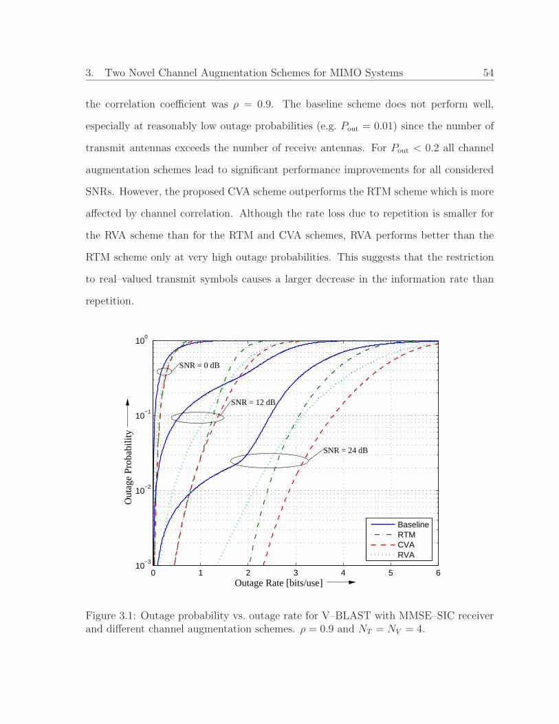
3. Two Novel Channel Augmentation Schemes for MIMO Systems 54
the correlation coefficient was ρ = 0.9. The baseline scheme does not perform well,
especially at reasonably low outage probabilities (e.g. Pout = 0.01) since the number of
transmit antennas exceeds the number of receive antennas. For Pout < 0.2 all channel
augmentation schemes lead to significant performance improvements for all considered
SNRs. However, the proposed CVA scheme outperforms the RTM scheme which is more
affected by channel correlation. Although the rate loss due to repetition is smaller for
the RVA scheme than for the RTM and CVA schemes, RVA performs better than the
RTM scheme only at very high outage probabilities. This suggests that the restriction
to real–valued transmit symbols causes a larger decrease in the information rate than
repetition.
0 1 2 3 4 5 610
−3
10−2
10−1
100
BaselineRTMCVARVA
SNR = 24 dB
Outage Rate [bits/use]
Out
age
Pro
babi
lity
SNR = 0 dB
SNR = 12 dB
Figure 3.1: Outage probability vs. outage rate for V–BLAST with MMSE–SIC receiverand different channel augmentation schemes. ρ = 0.9 and NT = NV = 4.

3. Two Novel Channel Augmentation Schemes for MIMO Systems 55
In Fig. 3.2, we investigate the impact of correlation on the various channel augmenta-
tion schemes if again V–BLAST with MMSE–SIC receiver is employed. NT = NV = 4,
Pout = 0.01, and SNRs of 12 and 24 dB are assumed. For the considered case, all three
schemes outperform the baseline scheme even for high correlations. While for SNR =
12 dB RTM and CVA have practically the same performance, for SNR = 24 dB the
higher robustness of CVA against channel correlation becomes obvious. Since for the
RVA scheme with NV = 4 only one repetition is necessary, it is even more robust against
channel correlations than the CVA scheme which requires three repetitions with complex
conjugation. However, for the considered scenario the outage rate of RVA is still lower
than that of CVA even for high correlations.
0 0.4 0.6 0.8 0.9 0.99
0.5
1
1.5
2
2.5
3
3.5
4
4.5
BaselineCVARTMRVA
Correlation Coefficient
Out
age
Rat
e [b
its/u
se]
SNR = 12 dB
SNR = 24 dB
Figure 3.2: Outage rate vs. correlation coefficient ρ for V–BLAST with MMSE–SICreceiver and different channel augmentation schemes. Pout = 0.01 and NT = NV = 4.

3. Two Novel Channel Augmentation Schemes for MIMO Systems 56
The effect of the number of transmit antennas and the number of virtual receive
antennas on outage performance is considered in Fig. 3.3 for optimum processing, i.e.,
for D–BLAST and an MMSE–SIC receiver. For comparison we have also included the
outage rate for maximum–rate full–diversity OSTBCs [62]. An outage probability of
Pout = 0.01, SNRs of (a) 0 dB, (b) 12 dB, and (c) 24 dB, and ρ = 0.6 were assumed.
For channel augmentation the proposed CVA scheme was adopted and the curves for
NV = 1 correspond to the baseline scheme without augmentation. Fig. 3.3 shows that
for the optimum transmitter and receiver structures the optimum value for NV strongly
depends on the SNR but is almost independent of NT . In particular, NV = 6 and NV = 2
are optimum for SNR = 0 dB and SNR = 12 dB for all considered NT . For SNR = 24
NV = 2 is optimum for NT > 2, while for NT = 2 the baseline scheme with NV = 1
performs slightly better. While OSTBCs achieve the same outage rate as the baseline
scheme for NT = 2, their performance deteriorates for NT > 2 due to their inherent rate
loss [62]. We note, however, that the decoding complexity of OSTBCs is lower than that
of the MMSE–SIC receiver required for D–BLAST with channel augmentation.
3.6 Conclusions
In this chapter, we have presented two simple channel augmentation schemes referred to
as CVA and RVA. We compared both schemes with the previously proposed RTM scheme
for the V–BLAST and D–BLAST architectures. Our results show that both the CVA
and the RVA schemes are more robust to channel correlations than the RTM scheme.
Furthermore, while all considered channel augmentation schemes can achieve signifi-
cantly higher outage rates than the baseline scheme without augmentation, the CVA
scheme outperformed the RVA and RTM schemes for all considered cases. Therefore,
the performance gains compared to the baseline scheme are larger for the suboptimum
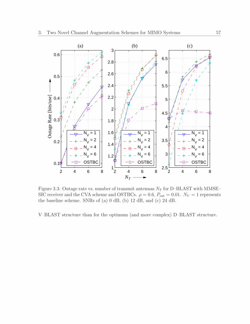
3. Two Novel Channel Augmentation Schemes for MIMO Systems 57
2 4 6 8
0.1
0.2
0.3
0.4
0.5
0.6
NV = 1
NV = 2
NV = 4
NV = 6
OSTBC
2 4 6 81
1.2
1.4
1.6
1.8
2
2.2
2.4
2.6
2.8
3
NV = 1
NV = 2
NV = 4
NV = 6
OSTBC
2 4 6 82.5
3
3.5
4
4.5
5
5.5
6
6.5
NV = 1
NV = 2
NV = 4
NV = 6
OSTBC
TN
Out
age
Rat
e [b
its/u
se]
(a) (b) (c)
Figure 3.3: Outage rate vs. number of transmit antennas NT for D–BLAST with MMSE–SIC receiver and the CVA scheme and OSTBCs. ρ = 0.6, Pout = 0.01. NV = 1 representsthe baseline scheme. SNRs of (a) 0 dB, (b) 12 dB, and (c) 24 dB.
V–BLAST structure than for the optimum (and more complex) D–BLAST structure.

58
4 On MIMO–OFDM with Coding
and Loading 1
4.1 Introduction
In the previous chapter, we have introduced two novel channel augmentation schemes
for MIMO systems. Starting from this chapter, we will focus on several aspects of signal
design specifical for MIMO–OFDM systems. We first present ABL schemes for coded
MIMO–OFDM in this chapter.
MIMO–OFDM schemes with ABL have been extensively studied recently [70, 79–
82] assuming different levels of CSI at the transmitter (perfect CSI at the receiver is
assumed). Kuhn et al. [79] and Li et al. [70] presented results for coded MIMO–OFDM
with ABL based on the SVD of the MIMO channel in case of full CSI. In [80] eigen–
beamforming is applied to uncoded transmission when only partial CSI is available.
V–BLAST [3] processing is often employed if CSI is not available at the transmitter
[81, 82]. This kind of MIMO processing without the need for CSI at the transmitter
is particularly interesting for moderately mobile applications as envisaged in e.g. IEEE
802.16e OFDM systems.
1The material in this chapter was presented in part at IEEE International Conference on Computer
Communications and Networks, Hawaii, USA, August 2007.

4. On MIMO–OFDM with Coding and Loading 59
In this chapter, we study pragmatic schemes for coded and bit–loaded MIMO–OFDM
which do not require CSI for MIMO processing at the transmitter and only a low–rate
feedback channel to perform ABL. Our contributions can be summarized as follows.
• We propose the application of wrapped space–frequency coding (WSFC), which is
the space–frequency counterpart of wrapped space–time coding (WSTC) devised in
[57], as efficient coding scheme for MIMO–OFDM without CSI. WSFC retains the
simplicity of V–BLAST, but alleviates the problem of error propagation by means
of a special formatting of coded symbols to transmitted symbols. Furthermore, we
optimize the WSFC decision delay for the considered application.
• For V–BLAST with ABL we devise a simple method to increase the performance
margin of the symbols corresponding to the antennas decoded first such that error
propagation is mitigated.
• While compared to SVD–based MIMO–OFDM, WSFC–based and V–BLAST–
based MIMO–OFDM requires already only little feedback for ABL, we explore
further feedback reduction using subchannel grouping methods.
• We present simulation results for practically relevant systems and channel param-
eters that show that MIMO–OFDM with optimized WSFC and V–BLAST and
reduced feedback for ABL achieve similar performances, which closely approach
that of SVD–based MIMO–OFDM.
The remainder of this chapter is organized as follows. Section 4.2 provides the system
model for MIMO–OFDM. Section 4.3 presents WSFC applied to MIMO–OFDM, and
reviews V–BLAST and SVD. Section 4.4 introduces adaptive bit–loading schemes and
describes the proposed modification for bit–loaded V–BLAST. Section 4.5 presents the
simulation results and discussion, and finally Section 4.6 gives the conclusions.

4. On MIMO–OFDM with Coding and Loading 60
4.2 System Model
The OFDM system under consideration is equipped with NT transmit and NR receive
antennas and we assume NT ≤ NR. The number of subcarriers is K. The block diagram
of the OFDM system with MIMO signal processing and adaptive bit loading is shown
in Fig. 4.1.
Sink
Encoding Interleaving
Decoding
ChannelEstimator
AdaptiveBit−
Loading
ProcessingMIMO Signal
N
1
RFFT
FFT
IFFTNT
1IFFT
Deinterleaving
Source bits
Feedback Channel
Channel
Channel
Figure 4.1: Block diagram of the MIMO–OFDM system with adaptive bit loading.(I)FFT denotes (inverse) fast Fourier transform.
At the transmitter, source bits are first encoded with a binary convolutional encoder
and possibly interleaved (see below). The coded bits are fed into the ABL unit, which
allocates bits to each of the K OFDM subcarriers and NT antennas. While ABL and
MIMO transmission are described in detail below, it should be noted that ABL requires
feedback from the receiver only in the form of a vector of integers which specifies the
number of bits assigned to each subcarrier and antenna. The amount of feedback for
loading is thus much smaller than that for providing full CSI to the transmitter as
required for MIMO processing with SVD.
Denoting xk , [xk,0 . . . xk,NT−1]T the NT –dimensional vector transmitted over NT

4. On MIMO–OFDM with Coding and Loading 61
antennas and subcarrier k, 0 ≤ k < K, and assuming standard OFDM transmission and
reception, the corresponding NR–dimensional received vector is given by
yk = Hkxk + nk , 0 ≤ k < K , (4.1)
with the NR × NT channel matrix Hk and the additive spatially and spectrally white
Gaussian noise nk. The MIMO–OFDM channel is assumed to be block fading, i.e.,
the channel does not change during one coding block, but may vary from one block to
another. We assume perfect CSI at the receiver (ideal channel estimator in Fig. 4.1).
4.3 MIMO Processing for Coded MIMO–OFDM
We now introduce the WSFC scheme for MIMO–OFDM with ABL (Section 4.3.1) and
briefly review V–BLAST-based (Section 4.3.2) and SVD-based MIMO–OFDM (Sec-
tion 4.3.3), cf. e.g. [79, 81].
4.3.1 Wrapped Space-Frequency Coding (WSFC)
WSFC is the straightforward extension of WSTC devised in [57] for single-carrier space-
time transmission to MIMO–OFDM. The coded bit stream is divided into NT layers
assigned to N = (K − (NT − 1)d)NT transmit symbols such that if cj, 0 ≤ j < K,
denotes the jth symbol mapped from the encoder output, then xk,i = cNT (k−id)+i for
id ≤ k < K − (NT − 1 − i)d and xk,i = 0 otherwise, 0 ≤ i < NT . The parameter d
is the so-called interleaving delay. This formatting “wraps” the codeword around the
space-frequency plane, skewed by the delay d. Fig. 4.2 shows an example of a WSFC
codeword matrix with NT = 3, d = 3, and K = 384 (cf. [57, Fig. 2] for WSTC). Note
that d = 3 is chosen only for illustration. The actual value for d needs to be optimized

4. On MIMO–OFDM with Coding and Loading 62
171411852
10 13 16741
93 60 11251128
112611291132
112711301133
12 15 1131
d
K
NT
Figure 4.2: Example of a WSFC codeword matrix with NT = 3, d = 3, and K = 384.The indices of the coded symbols are shown in the blocks.
for the best tradeoff between rate loss due to zero-symbols xk,i = 0 and error propagation
(see Section 4.5).
The skewness of the space-frequency arrangement of data symbols enables decod-
ing with per-survivor processing (PSP) at the receiver. The received vectors are first
processed with linear matrix-filters F k to form the vectors
vk , [vk,0 . . . vk,NT−1]T (4.2)
= F Hk yk (4.3)
= Bkxk + n′k, (4.4)
where Bk = F Hk Hk is the so-called feedback matrix and n′
k = [n′k,0 n′
k,1 . . . n′k,NT−1]
T is
the additive noise. This filtering is performed in the “MIMO Signal Processing” block of
Fig. 4.1. Usual choices for the matrix F k in MIMO processing are the whitened matched
filter, for which Bk would be upper triangular and nk would be spatially white Gaussian
noise, or the unbiased MMSE filter, in which case the elements of nk are correlated, cf.
[57, Section III]. Here, we consider the unbiased MMSE filter for its usually superior
performance and we approximate n′k as AWGN for the decoder design. Then, denoting
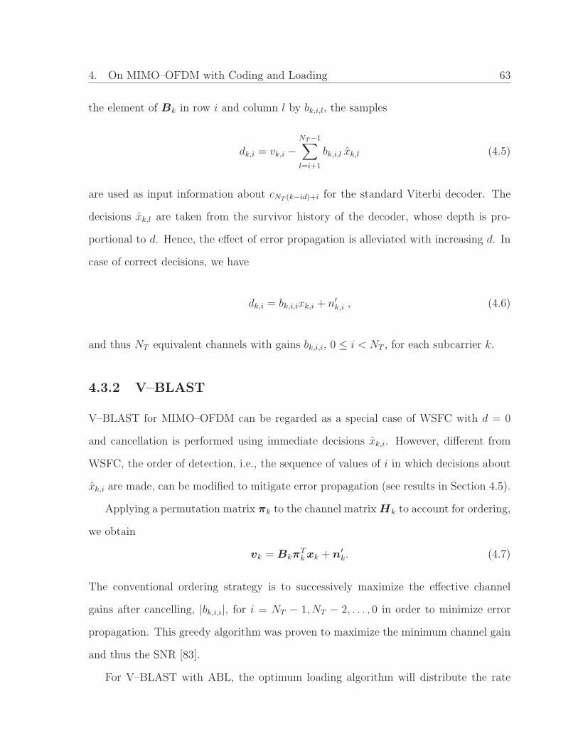
4. On MIMO–OFDM with Coding and Loading 63
the element of Bk in row i and column l by bk,i,l, the samples
dk,i = vk,i −NT−1∑
l=i+1
bk,i,l xk,l (4.5)
are used as input information about cNT (k−id)+i for the standard Viterbi decoder. The
decisions xk,l are taken from the survivor history of the decoder, whose depth is pro-
portional to d. Hence, the effect of error propagation is alleviated with increasing d. In
case of correct decisions, we have
dk,i = bk,i,ixk,i + n′k,i , (4.6)
and thus NT equivalent channels with gains bk,i,i, 0 ≤ i < NT , for each subcarrier k.
4.3.2 V–BLAST
V–BLAST for MIMO–OFDM can be regarded as a special case of WSFC with d = 0
and cancellation is performed using immediate decisions xk,i. However, different from
WSFC, the order of detection, i.e., the sequence of values of i in which decisions about
xk,i are made, can be modified to mitigate error propagation (see results in Section 4.5).
Applying a permutation matrix πk to the channel matrix Hk to account for ordering,
we obtain
vk = BkπTk xk + n′
k. (4.7)
The conventional ordering strategy is to successively maximize the effective channel
gains after cancelling, |bk,i,i|, for i = NT − 1, NT − 2, . . . , 0 in order to minimize error
propagation. This greedy algorithm was proven to maximize the minimum channel gain
and thus the SNR [83].
For V–BLAST with ABL, the optimum loading algorithm will distribute the rate

4. On MIMO–OFDM with Coding and Loading 64
to the equivalent channels such that their error rates are approximately equal (see Sec-
tion 4.4). In particular, the loading algorithm will always assign symbols from larger
signal constellations to spatial channels with higher gains without considering error prop-
agation. Hence, the optimum decoding order for V–BLAST with ABL could be different
from that for V–BLAST without ABL. In fact, it has been found in [84] that the near-
optimal decoding order for V–BLAST with ABL is obtained if the greedy algorithm
chooses the transmit antenna with the smallest equivalent gain among the remaining
unassigned antennas (cf. also [82]). In Section 4.4.3, we will describe a modification of
V–BLAST with ABL to further reduce error propagation.
In addition to ordering, with V–BLAST coded bits are interleaved before mapping
to (non-binary) signal points, which is not possible in case of WSFC due to the strict
correspondence between coded bits and space-frequency transmit symbols.
4.3.3 SVD
By performing SVD, the channel matrix Hk can be written as
Hk = U kΣkVHk , (4.8)
where U k and V Hk are unitary matrices. The entries of the diagonal matrix Σk, σk,0 ≥
σk,1 ≥ . . . ≥ σk,NT−1 ≥ 0, are the sorted non-negative singular values of Hk. In SVD-
based MIMO transmission, the matrices V k and UHk are applied to xk at the transmitter
and yk at the receiver, respectively. This generates NT parallel channels with gains σk,i,
0 ≤ i < NT , for each subcarrier k. As for V–BLAST, coding with bit-interleaving can
be applied. We note that, different from WSFC and V–BLAST, full knowledge of Hk
is necessary to perform SVD-based transmission.
4. On MIMO–OFDM with Coding and Loading 65
4.4 Adaptive Bit-Loading (ABL) Schemes
A number of loading algorithms have been proposed for single-antenna OFDM systems,
cf. [35–40], and most of them achieve quite similar performance-complexity tradeoffs.
In this chapter, we are interested in constant throughput and thus apply the margin-
adaptive loading algorithm by Chow, Cioffi and Bingham (CCB) [36], whose information-
theoretic capacity criterion seems to be a good match for coded transmission (although
the codes considered in Section 4.5 do not operate at the capacity limit). However,
numerical results not shown here indicate that the choice of the particular loading algo-
rithm is not critical for coded MIMO–OFDM.
Since the MIMO processing schemes described in the previous section lead to an
overall system with NT K parallel channels (assuming perfect cancellation for WSFC and
V–BLAST), the CCB algorithm can be directly applied. We first consider two versions of
loading with different feedback requirements and computational complexities and then
describe a modification of the loading algorithm to account for error propagation in
V–BLAST.
4.4.1 Full Loading (FL)
This scheme allocates bits to all NT K equivalent channels individually without distin-
guishing between spectral or spatial dimensions.
4.4.2 Grouped Loading (GL)
This scheme forms groups of equivalent channels with similar channel gains and the
loading algorithm considers all channels within a group as identical. Since the channel
gains bk,i,i (WSFC/V–BLAST) and σk,i (SVD) are typically highly correlated along the
frequency axis (index k) but strongly vary in the spatial domain (index i), grouping

4. On MIMO–OFDM with Coding and Loading 66
of G adjacent subcarriers corresponding to the same transmit antenna is proposed.
G is referred to as the group size. To provide the loading algorithm with a group
representative, we consider two methods:
Center subcarrier method
The center subcarrier of the group (or one of the center subcarriers if G is even) represents
the group.
Equivalent SNR method
A virtual channel whose SNR equals
SNReq = Γγ
[
G−1∏
l=0
(
1 +SNRl
Γγ
)1/G
− 1
]
, (4.9)
where SNRl is the SNR for the lth subcarrier in the group, Γ is the “SNR gap” and γ
is the system performance margin iteratively updated by the CCB algorithm, cf. [36].
Eq. (4.9) directly derives from averaging the capacities (see [36, Eq. (1)]) associated with
the subcarriers in the group.
Since GL reduces the required amount of feedback by a factor of G, it is a very
interesting alternative, especially for WSFC/V–BLAST OFDM, which do not require
CSI at the transmitter for MIMO processing. A virtual channel whose capacity equals
the mean of the capacities of the channels in the group represents the group.
4.4.3 Modification of Loading for V–BLAST
As described in Section 4.3.2, the effect of error propagation in V–BLAST with ABL
is mitigated by sorting the spatial subchannels in the order of increasing channel gains.
It seems, however, advisable to also take error propagation into account when actually

4. On MIMO–OFDM with Coding and Loading 67
performing the loading. More specifically, we propose to increase the performance mar-
gin for the symbols of the antennas decoded first in the bit loading algorithm, which
makes the tentative decisions of V–BLAST more reliable. To this end, we introduce a
parameter, the extra margin ηi, 0 ≤ i < NT , and make the following modification to the
CCB algorithm. We replace Eq. (1) of [36] with
bk,i = log2
(
1 +SNRk,i
Γγη2i
)
, (4.10)
where bk,i, SNRk,i, and ηi are the number of bits allocated, the SNR, and the extra
performance margin of the ordered i-th symbol on subcarrier k, respectively.
If we set η0 = 1, then ηi, 0 < i < NT , become the extra margins relative to the
last detected symbol for a certain subcarrier k. The remaining task is to find the ηi
that minimizes the overall error rate. Since the parameter space increases exponentially
with NT , we propose the pragmatic choice ηi = (ηextra)i, 0 ≤ i < NT , where ηextra ≥ 1
is the only parameter to be optimized. This will be done in the next section based on
simulated performances.
4.5 Results and Discussion
We now present and discuss simulation results for the different MIMO–OFDM schemes
with ABL. We adopt the following system parameters from the IEEE 802.16e standard
[6]: OFDM with 3.5 MHz bandwidth and 512 subcarriers of which 384 are active; rect-
angular M–QAM constellations with M = 2i, 0 ≤ i ≤ 8, and Gray labelling of signal
points; convolutional encoder with generator polynomials (171, 133)8. We further as-
sume NT = NR = 2 as a relevant example, and the ITU–R vehicular channel model A
[85]. In all cases, the average data rate per active subcarrier is fixed to R = 2 bits and

4. On MIMO–OFDM with Coding and Loading 68
R = 4 bits, respectively.
4.5.1 Optimization of WSFC and V–BLAST for MIMO–OFDM
with ABL
First, we consider the optimization of WSFC. Fig. 4.3 shows the SNR Es/N0 required
for a BER of 10−3 versus the interleaving delay d. While increasing d leads to more
accurate tentative decisions it also incurs a larger rate loss due to initialization and
termination of WSFC encoding. In order to keep the overall rate unchanged, more
bits have to be allocated to subcarriers not affected by initialization and termination,
which has a negative effect on BER performance. In the case of R = 2 bits, the system
achieves the best performance when the delay lies in the range from d = 16 to d = 32.
For R = 4 bits, the best performance is obtained between d = 8 and d = 28. Hence,
d = 16 is a universally good choice and used in the following. We note, however, that
somewhat smaller (larger) delays may be optimal for OFDM with fewer (more) than 384
subcarriers due to the more (less) pronounced rate loss for fixed d.
Next, we consider the optimization of bit-loaded V–BLAST with ordering, where
the symbol assigned to the spatial channel with the smallest gain will be decoded first.
Fig. 4.4 shows the SNR Es/N0 required for BERs of 10−3 and 10−4 versus the extra
margin ηextra for the case of R = 2 bits. The curves for V–BLAST without ordering are
also included as references. Using an extra margin, ηextra > 1, leads to more reliable
tentative decisions, however, it also makes the symbols corresponding to the antenna
detected last more error-prone. It can be seen that the optimum extra margins are
approximately at ηextra = 2 ∼ 2.5 and that optimization with respect to ηextra provides
gains of 0.7 dB at BER = 10−3 and 1.3 dB at BER = 10−4, respectively. This is quite
remarkable considering that the improvement due to ordering (i.e. ηextra = 1) is only

4. On MIMO–OFDM with Coding and Loading 69
0 2 4 6 8 12 16 20 24 28 32 40 486
7
8
9
10
11
12
13
14
15
16
17
18
19
202 bits4 bits
10lo
g10(E
s/N
0)
for
BE
R=
10−
3−→
d −→
Figure 4.3: SNR required for WSFC to achieve BER = 10−3 vs. interleaving delay dwith R = 2 bits and 4 bits.
0.25 and 0.9 dB, respectively.
4.5.2 Performance Comparisons
We now compare the performances of coded MIMO–OFDM based on SVD, V–BLAST,
and WSFC. To separate the different effects, (i) V–BLAST without ordering, (ii) V–
BLAST with ordering, and (iii) V–BLAST with ordering and optimal ηextra are consid-
ered. Note that bit-interleaving is applied for V–BLAST but not for WSFC.
Fig. 4.5 shows the BER results for R = 2 bits with and without ABL. As expected,
SVD with ABL yields the best performance among all the schemes and its bit-loading
gain is more than 8.4 dB at BER = 10−4. Interestingly, SVD without loading is inferior
to WSFC, which can be attributed to the large variations of the subchannel gains in
case of SVD. WSFC with ABL approaches the performance of SVD within 1.2 dB, and

4. On MIMO–OFDM with Coding and Loading 70
1 1.5 2 2.5 3 3.5 4 4.5 58.5
9
9.5
10
10.5
11
11.5
12V−BLAST without orderingV−BLAST with ordering
BER = 10−4
BER = 10−3
10lo
g10(E
s/N
0)
for
BE
R=
10−
3an
dB
ER
=10
−4
−→
ηextra −→
Figure 4.4: BER required for V–BLAST with and without ordering vs. extra marginηextra .
its loading gain is 1.5 dB at BER = 10−4. WSFC clearly outperforms V–BLAST, which
confirms the effectiveness of the interleaving delay d. If the detection order is optimized,
the performance of V–BLAST with ABL is 2.1 dB worse than that of WSFC. If the
proposed additional margin ηextra is applied for ABL, the SNR gap between V–BLAST
and WSFC decreases to 0.8 dB at BER = 10−4.
Finally, we consider the performance if GL is applied for the example of R = 2 bits.
For V–BLAST (with ordering), ABL without and with extra margin is performed.
Fig. 4.6 shows the results in terms of the SNR required to achieve a BER of 10−3
for group sizes of G = [1, 2, 4, 8]. The SNR values for transmission without loading are
also given as a reference. It can be seen that WSFC is more robust to the suboptimal-
ity due to grouping than V–BLAST. The larger deterioration for V–BLAST should be
attributed to the aggravated error propagation when employing non-ideal loading. This

4. On MIMO–OFDM with Coding and Loading 71
0 2 4 6 8 10 12 14 16 18 2010
−5
10−4
10−3
10−2
10−1
SVDSVD ABLV−BLAST without orderingV−BLAST ABL without orderingV−BLAST ABL with orderingV−BLAST ABL with ordering and η
extra
WSFCWSFC ABL
BER
−→
10 log10(Es/N0) −→
Figure 4.5: BER performance for coded MIMO–OFDM with and without ABL. R =2 bits, and d = 16 for WSFC.
effect is alleviated in case of WSFC due to the interleaving delay d > 0. For WSFC
the SNR-penalties compared to G = 1 are [0.05, 0.16, 0.53] dB when using the center
subcarrier and only [0.02, 0.09, 0.3] dB when using the equivalent SNR for ABL. The
latter criterion is apparently advantageous for WSFC and losses of e.g. 0.09 and 0.3 dB
are fairly small given the reduction in feedback required for loading by factors of 4 and
8, respectively. Interestingly, for V–BLAST the center-subcarrier criterion yields better
performances, which shows that one should not blindly apply a certain criterion for ABL
with grouping of subcarriers.
We conclude that both optimized WSFC and V–BLAST achieve power efficiencies
close to that of SVD-based MIMO–OFDM with ABL, and WSFC is somewhat advan-
tageous if the feedback channel required for ABL has a very limited capacity.

4. On MIMO–OFDM with Coding and Loading 72
8 8.5 9 9.5 10 10.5 11 11.5 12 12.5 13
G=1G=2G=4G=8no loading
Diff
eren
t MIM
O−
OF
DM
and
Loa
ding
Met
hods WSFC, equivalent SNR
WSFC, center subcarrier
10 log10(Es/N0) −→
V-BLAST without ηextra, equivalent SNR
V-BLAST with ηextra, center subcarrier
V-BLAST with ηextra, equivalent SNR
V-BLAST without ηextra, center subcarrier
Figure 4.6: SNR required to achieve BER = 10−3 for WSFC and V–BLAST with orderingbased MIMO–OFDM with different group sizes G for ABL. R = 2 bits, and d = 16 forWSFC. The center subcarrier and equivalent SNR methods are used for loading.
4.6 Conclusions
In this chapter, we have studied coded MIMO–OFDM with ABL. We have proposed
WSFC for MIMO–OFDM and a modified loading for V–BLAST to mitigate the problem
of error propagation. Furthermore, we have considered ABL with subcarrier grouping
based on two criteria to reduce the feedback load. The presented simulation results have
shown notable gains due to WSFC and V–BLAST optimization, and that WSFC and
V–BLAST perform fairly close to the benchmark case of SVD, which requires full CSI at
the transmitter. We thus conclude that the devised WSFC-based and V–BLAST–based
MIMO–OFDM with ABL are attractive solutions for power and bandwidth-efficient
transmission for scenarios with small feedback rates like in e.g. IEEE 802.16e systems.
73
5 Cyclic Space–Frequency Filtering
for BICM–OFDM Systems 1
5.1 Introduction
In Chapter 4, we have studied coded MIMO–OFDM with ABL, which requires small
feedback of instant parameters for ABL from the receiver. In this chapter, we intro-
duce cyclic space–frequency (CSF) filtering, a SFC scheme, which exploits the space
and frequency diversity of MIMO–OFDM without requiring instant feedback from the
receiver.
OFDM converts a frequency–selective fading channel into a number of parallel flat
fading channels. As mentioned before, the negative effects of flat fading can be reduced
with multiple transmit and multiple receive antennas and application of some form of
SFC, cf. e.g. [45, 48]. Thereby, the multiple transmit antennas may either belong to the
transmitting user (source node) or to other users who act as relay nodes to form a virtual
MIMO system [20]. In this chapter, we refer to the former and the latter scenarios as
transmission with co–located and distributed antennas, respectively. In the distributed
case, we assume a two–hop protocol with DF relays [20]. A particularly simple and
1The material in this chapter was presented in part at IEEE Vehicular Technology Conference (VTC–Fall), Baltimore, USA, October 2007, and in part at VTC–Spring, Singapore, May 2008.

5. Cyclic Space–Frequency Filtering for BICM–OFDM Systems 74
efficient form of SFC, which is applicable to both co–located [49, 50] and distributed [86]
transmit antennas, is CDD, cf. Section 2.5. CDD is typically combined with BICM [44]
which is capable of exploiting the additional frequency diversity created by CDD and
widely used in existing wireless standards [87].
The proposed CSF filtering schemes can be applied for BICM–OFDM systems with
multiple co–located or distributed transmit antennas. CSF filtering may be viewed as
a generalization of CDD where the cyclic delays are replaced by CSF filters. Unlike in
conventional SFC schemes, the CSF filters are not defined over a finite field but over the
field of complex numbers. The contributions made in this chapter can be summarized
as follows:
• Assuming BICM at the transmitter and Viterbi decoding at the receiver, we de-
velop optimization criteria for CSF filtering with co–located and distributed trans-
mit antennas, respectively.
• Based on these criteria we present closed–form solutions for the optimum CSF
filters for several special cases and numerical methods for efficient CSF filter design
for the general case, where closed–form solutions do not exist.
• We show that BICM–OFDM with CSF filtering can exploit the full spatial and
spectral diversity of wireless systems with co–located or distributed antennas.
• We also discuss the extension of our results to OFDMA systems.
There is a large body of literature on finite field based SFC schemes for co–located,
e.g. [45, 46, 88, 89], and distributed, e.g. [65, 90–93], transmit antennas. In contrast
to these schemes, the proposed CSF filtering scheme, if properly designed, does not
require any changes to the receiver compared to single–antenna transmission. This is a
major advantage in networks where devices with different numbers of antennas have to

5. Cyclic Space–Frequency Filtering for BICM–OFDM Systems 75
coexist and facilitates the upgrade of existing wireless systems. For example, to provide
transmit diversity in the downlink only the access points have to be equipped with CSF
filters and multiple antennas but the user devices do not have to be modified. Recently,
several attempts have been made to optimize CDD for co–located antennas. In [87],
CDD with large cyclic delays is advocated and the interleaver is optimized accordingly.
Precoding for CDD was proposed in [94] and optimized for uncoded transmission. The
idea of replacing the cyclic delays with cyclic filters has been proposed independently
in [95].2 However, [95] advocates a relatively complex simulation–based approach to
filter optimization whereas we derive a simple closed–form optimality criterion. The
optimization of CDD for cooperative OFDM transmission with distributed antennas was
discussed in [50]. We finally note that there are several related papers which optimize
linear DD and/or linear space–time filtering for uncoded single–carrier transmission with
co–located [96, 97] and distributed [65, 98] antennas.
The remainder of this chapter is organized as follows. In Section 5.2, the system
models for co–located and distributed CSF filtering are introduced. The optimization of
the CSF filters when the set of transmit antennas is known and not known is presented
in Sections 5.3 and 5.4, respectively. In Section 5.5, simulation results are provided, and
Section 5.6 concludes this chapter.
5.2 System Model
In this section, we introduce the considered network, transmitter, channel, and receiver
models.
2Both the conference version of this chapter and [95] were presented at IEEE VTC–Fall 2007.
5. Cyclic Space–Frequency Filtering for BICM–OFDM Systems 76
5.2.1 Network Model
We consider a BICM–OFDM system with K subcarriers, NR receive antennas, and NT
co–located or distributed transmit antennas.
Co–located Antennas: In this case, we assume a simple point–to–point transmission
where transmitter and receiver are equipped with NT and NR antennas, respectively.
Distributed Antennas: We consider a network with one source node, one destina-
tion node, and N relay nodes. Each relay node is assigned a number n ∈ N ,N ,
1, 2, · · · , N. Furthermore, the source and relay nodes are equipped with a single an-
tenna, whereas the destination node has NR antennas. We adopt a commonly used
two–phase protocol [20]. During the first phase, the source node broadcasts a data
packet to the relay nodes, and there is no transmission from the source to the destina-
tion node. During the second phase (relay phase), only those NT ≤ N relay nodes which
can successfully decode the packet received from the source in the first phase forward the
packet to the destination node, cf. Fig. 5.1. The relay nodes participating in the second
phase of transmission are collected in the set of active nodes S = n1, . . . , nNT ⊆ N ,
|S| = NT . We consider both coordinated and uncoordinated relaying. In coordinated
relaying, the transmitting relay nodes know S (i.e., they know which other nodes are ac-
tive), whereas in uncoordinated relaying, the relay nodes do not know S. Uncoordinated
relaying requires less overhead since the active relay nodes do not have to communicate
with each other.
5.2.2 Transmitter
Block diagrams of the proposed transmitter structure for co–located and distributed
antennas are shown in Figs. 5.2a) and b), respectively.

5. Cyclic Space–Frequency Filtering for BICM–OFDM Systems 77
S D
1
32
8
9
7
5
6 10
4
Figure 5.1: Example of a simple two–phase transmission with N = 10 potentially co-operating relay nodes. NT = 4 relay nodes (S = 1, 3, 9, 10) successfully decode thepacket received from the source node (S) and forward it to the destination node (D).
MapperΠ IFFTCC
b)
a)
... ......
CP
CP
CP
MapperΠ IFFTCC
ck′sn[t]
gn
gNT
g1
X[k]
X[k]
x[t]
s1[t]
sNT[t]
ck′
x[t]
Figure 5.2: Block diagram of a) transmitter with NT co–located antennas employingBICM–OFDM and CSF filtering, and b) transmitter of the nth relay node employingBICM–OFDM and CSF filtering.

5. Cyclic Space–Frequency Filtering for BICM–OFDM Systems 78
Co–located Antennas: The bit stream is encoded with a convolutional encoder (CC)
which has rate R and free distance dfree. The K log2(M) coded bits ck′ , 1 ≤ k′ ≤
K log2(M) are interleaved and mapped onto symbols X[k], 1 ≤ k ≤ K, taken from
an M–ary symbol constellation X such as M–ary phase-shift keying (M–PSK) or M–
ary quadrature amplitude modulation (M–QAM). The effect of the interleaver Π can
be modeled by k′ → (k, i) where k′ denotes the original index of coded bit ck′ , and
k and i denote the index of symbol X[k] and the position of ck′ in the label of X[k],
respectively. We assume that the interleaver is chosen such that coded bits ck′1
and
ck′2
with |k′1 − k′
2| ≤ dfree are mapped onto different symbols which are transmitted over
different subcarriers. This is necessary to exploit the full diversity offered by the channel,
cf. [48]. Next, an IFFT is performed which converts frequency–domain symbols X[k],
1 ≤ k ≤ K, into time–domain symbols x[t], 1 ≤ t ≤ K.
At transmit antenna n, 1 ≤ n ≤ NT , the symbols x[t] are passed through CSF filter
gn , [gn[0] gn[1] . . . gn[Lg − 1]]T of length Lg ≤ K. The vector g , [gT1 . . . gT
NT]T
containing all CSF filter coefficients is normalized to ||g||2 = 1. The CSF filter output
at antenna n is given by
sn[t] = gn[t] ⊛ x[t] =
Lg−1∑
ν=0
gn[ν]x[(t − ν)K ], (5.1)
where ⊛ denotes the cyclic convolution operator. We note that conventional CDD with
delay D may be interpreted as a special case of the CSF filtering operation described
in (5.1) with gn[ν] = 1/√
NT for ν = (n − 1)D and gn[ν] = 0 otherwise. Before the
symbols sn[t] are transmitted by antenna n, a CP is added. We note that the CSF
filtering in (5.1) has no implications for the required length of the CP which – similar
to single–antenna transmission and CDD – is determined only by the length of the CIR.
Furthermore, similar to CDD, and in contrast to other SFC schemes, only one IFFT

5. Cyclic Space–Frequency Filtering for BICM–OFDM Systems 79
has to be performed at the transmitter. However, CSF filtering has a higher complexity
than CDD since it requires NT cyclic filtering operations whereas for CDD only NT
cyclic delays are necessary.
Distributed Antennas: The processing at active node n ∈ S is identical to the pro-
cessing at antenna n in the co–located antenna case, i.e., the transmit signal (before the
CP is added) is given by (5.1). All active relay nodes employ identical CCs, interleavers,
and mappers but in general different CSF filters gn. In case of coordinated relaying
the CSFs gn, n ∈ S, are optimized for the given set S, cf. Section 5.3. In contrast, for
uncoordinated relaying, the CSF filters gn, 1 ≤ n ≤ N , are optimized for all nodes in N
and do not depend on S (which is assumed to be unknown), cf. Section 5.4. We adopt
the power constraint ||gS ||2 = 1, where gS , [gTn1
. . . gTnNT
]T , for coordinated relaying.
For uncoordinated relaying a stricter per–node power constraint ||gn||2 = 1/NT , n ∈ S,
is adopted since S is not known.
For the following, we formally define S , 1, 2, . . . , NT for the co–located antenna
case, which enables a unified treatment of the channel models and the receiver processing
for CSF filtering with co–located and distributed transmit antennas.
5.2.3 Channel Model
We consider a frequency–selective channel with CIR hnr[l], 0 ≤ l ≤ L − 1, of length
L between transmit antenna n and receive antenna r. For convenience we collect the
corresponding CIR coefficients in vector hnr , [hnr[0] . . . hnr[L − 1]]T . The CIR coeffi-
cients are modeled as possibly correlated zero–mean complex Gaussian random variables
(Rayleigh fading).
We define the vector containing all CIR coefficients as hS , [hTn11 hT
n21 . . . hTnNT
NR]T .
For the channel autocorrelation matrix we adopt the popular Kronecker model, i.e.,

5. Cyclic Space–Frequency Filtering for BICM–OFDM Systems 80
Chh , EhShHS = CNR
⊗ CNT⊗ CL, where CNR
, CNT, and CL denote the receive
antenna, the transmit antenna, and the temporal autocorrelation matrices, respectively.
Temporal correlation may be introduced by transmitter and receiver filtering. For co–
located transmit antennas the off–diagonal elements of CNTwill be in general non–zero
due to spatial correlation. In contrast, for distributed transmit antennas CNTwill be
a diagonal matrix but its main diagonal elements may not be identical because of non–
identical relay–destination distances.
For both co–located and distributed transmit antennas we assume the channel to be
constant for the duration of at least one OFDM symbol and the autocorrelation matrix
to have full rank, i.e., r(CNR) = NR, r(CNT
) = NT , and r(CL) = L.
5.2.4 Receiver Processing
At the receiver, CSF filtering does not require any modifications compared to CDD and
single–antenna transmission. Assuming that the CP has a length of at least L− 1, after
removal of the CP and FFT the received signal at antenna r, 1 ≤ r ≤ NR, can be
expressed as
Rr[k] = Heq,r[k]X[k] + Nr[k], 1 ≤ k ≤ K, (5.2)
where the channel coefficient Heq,r[k] is given by Heq,r[k] =∑
n∈S Hnr[k]Gn[k], with
Hnr[k] ,∑L−1
l=0 hnr[l]e−j2πkl/K and Gn[k] ,
∑Lg−1l=0 gn[l]e−j2πkl/K , and Nr[k] is AWGN
with variance σ2n , E|Nr[k]|2. Next, optimum maximum ratio combining of the re-
ceived signals in each subcarrier is performed. The combined signal
R[k] =
NR∑
r=1
H∗eq,r[k]Rr[k], 1 ≤ k ≤ K, (5.3)

5. Cyclic Space–Frequency Filtering for BICM–OFDM Systems 81
is then used for bit metric calculation for the coded bit ck′ [44, 48]
λi(R[k], ck′) = minX∈X i
ck′
∣
∣
∣R[k] −
NR∑
r=1
|Heq,r[k]|2X∣
∣
∣
2
, (5.4)
where X ib denotes the subset of all symbols X ∈ X whose label has the value b ∈ 0, 1
in position i. The bit metrics are de–interleaved and Viterbi decoded [44, 48].
Remark: Eq. (5.2) shows that CSF filtering transforms the MIMO channel into
an equivalent single–input multiple–output (SIMO) channel with frequency response
Heq,r[k] for receive antenna r, 1 ≤ r ≤ NR. This corresponds to effective SIMO CIRs
heq,r[l] of length Leq = L + Lg − 1. Note that, in general, Heq,r[k] will contain more
spectral degrees of freedom than Hnr[k] because of the CSF filtering. The receiver
can directly estimate the equivalent overall CIRs heq,r[l] using one of the numerous
existing techniques for channel estimation in SIMO OFDM systems, cf. e.g. [99]. Direct
estimation of heq,r[l] is particularly convenient for distributed antennas since the receiver
does not have to know the set of active nodes S. However, even for co–located antennas
it may be advisable to directly estimate the NRLeq coefficients of the equivalent SIMO
channel instead of the NT NRL coefficients of the MIMO channel as long as Leq ≤ NT L.
Thus, as far as channel estimation is concerned, small Lg are preferable since they result
in short equivalent CIRs.
5.2.5 Extension to OFDMA
Similar to CDD [86, 87], CSF filtering can be easily extended to OFDMA systems. In
the following, we briefly point out the necessary modifications.
Co–located Antennas: For co–located antennas, the data streams of U users are
separately encoded, interleaved, mapped, and assigned to mutually exclusive sets of
K/U subcarriers. Subsequently a joint IFFT is applied to all K frequency domain

5. Cyclic Space–Frequency Filtering for BICM–OFDM Systems 82
symbols, cf. [87, Fig. 6]. The resulting time–domain sequence x[t], 1 ≤ t ≤ K, is applied
to the inputs of the NT CSF filters as shown in Fig. 5.2a).
Distributed Antennas: In the distributed case, U source nodes communicate with
up to U destination nodes at the same time using mutually exclusive sets of subcarriers
[86]. The nth relay node tries to decode the received packets of all U users, and forwards
the successfully decoded packets to the destination node(s) using OFDMA. Thereby, the
packets received from different sources are separately encoded, interleaved, mapped, and
assigned to mutually exclusive sets of K/U subcarriers. The subcarriers of unsuccessfully
decoded source nodes remain unmodulated. After the IFFT, CSF filtering is applied as
shown in Fig. 5.2b).
The received signals Rr[k], 1 ≤ r ≤ NR, belonging to different users/source nodes are
processed separately using the standard procedure outlined in Section 5.2.4. The CSF
filter optimization for BICM–OFDM presented in Sections 5.3 and 5.4 is – with minor
modifications – also applicable to BICM–OFDMA. We will point out these modifications
wherever necessary.
5.3 CSF Filter Optimization for Known S
In this section, we assume that S is known, which applies to co–located antennas
and coordinated relaying. A unified treatment is possible by adopting again S =
1, 2, . . . , NT for the co–located antenna case. We assume that the correlation matri-
ces CNTand CL are known and optimize the CSF filters accordingly. For simplicity of
notation, in this section, we replace gS with g, since S is fixed and known.
5. Cyclic Space–Frequency Filtering for BICM–OFDM Systems 83
5.3.1 Optimization Criterion
The proposed optimization criterion is based on the worst–case PEP of the considered
transmission system. From (5.3) we observe that for a given subcarrier and a given
channel realization the overall system including maximum ratio combining is equivalent
to a SISO system with SNR[k] = |Heq[k]|2/σ2n, 1 ≤ k ≤ K, where
|Heq[k]|2 ,
NR∑
r=1
|Heq,r[k]|2 =
NR∑
r=1
∣
∣
∣
∣
∣
∑
n∈SHnr[k]Gn[k]
∣
∣
∣
∣
∣
2
. (5.5)
Therefore, we can exploit the results presented in [48, Section IV], where the PEP of
BICM–OFDM was recently derived. In particular, exploiting [48, Eq. (7)] and Q(x) ≤
0.5e−x2/2 the PEP of two codewords c and c conditioned on hS and g can be upper
bounded as
P (c → c|hS , g) ≤ 1
2exp
(
−d2min
4σ2n
∑
k,dfree
|Heq[k]|2)
, (5.6)
where dmin denotes the minimum Euclidean distance of the signal constellation X and the
sum in the argument of the exponential function in (5.6) is over dfree distinct subcarriers
K , k1, k2, . . . , kdfree.3 For the following, it is helpful to rewrite this sum as
∑
k,dfree
|Heq[k]|2 =∑
k,dfree
NR∑
r=1
∣
∣
∣
∣
∣
∑
n∈SwH [k]Gnhnr
∣
∣
∣
∣
∣
2
= hHS (INR
⊗ GHWG)hS , (5.7)
where w[k] , [1 ej2πk/K . . . ej2πk(Leq−1)/K ]T , W ,∑
k,dfree
w[k]wH [k], G , [Gn1. . . GnNT
],
and Gn is an Leq ×L column–circular matrix with vector [gTn 0T
L−1]T in its first column.
Using (5.7) in (5.6) and averaging the PEP with respect to hS yields
P (c → c|g) ≤ 1
2
[
det
(
INRLeq+
d2min
4σ2n
(CNR⊗ WG(CNT
⊗ CL)GH)
)]−1
. (5.8)
3We note that in OFDMA the possible sets K are user dependent.

5. Cyclic Space–Frequency Filtering for BICM–OFDM Systems 84
Introducing the definition M , G(CNT⊗CL)GH and assuming σ2
n ≪ 1, we can rewrite
(5.8) as
P (c → c|g) ≤ 1
2[det(CNR
)]−r(WM)
[
r(WM)∏
i=1
λi(WM )
]−NR (
d2min
4σ2n
)−d
, (5.9)
where d , NRr(WM ) denotes the diversity gain. Assuming dfree ≤ K and Leq ≤ K, 4
we obtain r(W ) = mindfree, Leq, cf. e.g. [48, Appendix], and r(M ) = minLeq, NT L.
For the rank of the product WM the inequality
r(W ) + r(M ) − Leq ≤ r(WM ) ≤ minr(W ), r(M ) (5.10)
holds [100], where the upper bound is achievable if W and/or M are not singular. We
conclude from (5.9) that the achievable diversity gain with CSF filtering is
d = NR · mindfree, Leq, NT L. (5.11)
The coding gain of BICM–OFDM with CSF filtering can be defined as
C(g) ,
(
r(WM)∏
i=1
λi(WM )
)1/r(WM)
, (5.12)
cf. (5.9). To minimize the asymptotic PEP in (5.9), the CSF filters have to simultane-
ously maximize the coding gain C(g) and the diversity gain d. Note that (5.11) implies
that for given dfree, NT , and L the maximum possible diversity gain can be exploited
with CSF filters of length Lg,min = min(NT − 1)L + 1, dfree − L + 1. Increasing Lg
(and consequently Leq) further does not improve d but may increase C(g) and will sig-
4If OFDMA is employed, we have to assume dfree ≤ K/U and Leq ≤ K/U , respectively.

5. Cyclic Space–Frequency Filtering for BICM–OFDM Systems 85
nificantly impact the design of the optimal g. Therefore, we consider two different cases
for Lg in the following.
Case 1 [Lg ≤ Lg,min]: In this case, Leq ≤ mindfree, NT L and d = NRLeq are valid
and we can rewrite the coding gain as C(g) = (det(W ) det(M ))1/Leq , which implies that
we can optimize the interleaver (which influences W ) and the CSF filters separately. In
particular, for a given interleaver it suffices to maximize the cost function
f(g) , det(M ) = det(G(CNT⊗ CL)GH) (5.13)
subject to the power constraint ||g||2 = 1.
Case 2 [Lg > Lg,min]: In this case, we obtain Leq > mindfree, NT L and d =
NR mindfree, NT L, and (5.12) cannot be further simplified. Therefore, the interleaver
and the CSF filters have to be optimized jointly. Based on (5.10) it can be shown that
for mindfree, NT L < Leq ≤ maxdfree, NT L maximum–rank W and M guarantee a
diversity order of d = NR mindfree, NT L. This means if we choose to optimize/design
W and M separately, we are guaranteed to achieve full diversity but the coding gain
may not be maximized. On the other hand, for Leq > maxdfree, NT L we obtain from
(5.10) NR(NT L + dfree − Leq) ≤ d ≤ NR mindfree, NT L, which means that in this case
maximum–rank W and M do not even guarantee full diversity. This latter case was
considered for the CDD scheme in [87], where it was indeed found that the interleaver
and the cyclic delays have to be designed jointly.
Considering the above discussion, we will concentrate on Case 1 (Lg ≤ Lg,min) in
the remainder of this section. This allows us to optimize the CSF filters indepen-
dent from the interleaver, which is a major advantage. Note that this choice does
not compromise the diversity gain since Lg = Lg,min exploits the maximum diversity
gain d = NR mindfree, NT L of the BICM–OFDM system. Choosing Lg > Lg,min yields

5. Cyclic Space–Frequency Filtering for BICM–OFDM Systems 86
additional coding gains which, however, tend to be small if S is known, cf. discussion of
Fig. 5.6.
5.3.2 Upper Bound on Cost Function f(g)
In this section, we derive an upper bound on f(g). For this purpose we assume that
G is a general Leq × NT L matrix (without a pre–defined structure), which only has to
fulfill the power constraint trGHG = L. For clarity we denote the corresponding cost
function by f(G) = det(G(CNT⊗ CL)GH). It can be shown that the maximum value
of f(G) is given by
f(Gopt) =
(
L
Leq
)LeqLeq∏
i=1
λi(CNT⊗ CL) (5.14)
with optimum matrix Gopt =√
LLeq
UHLeq
, where the unitary NT L × Leq matrix ULeq
contains the eigenvectors (EVs) of CNT⊗CL corresponding to the Leq largest eigenval-
ues.
Since the CSF filter matrix G does not only have to fulfill a power constraint but
the sub–matrices Gnm, 1 ≤ m ≤ NT , also have to be cyclic, cf. Section 5.3.1, f(g) can
be bounded as
f(g) ≤(
L
Leq
)LeqLeq∏
i=1
λi(CNT⊗ CL) (5.15)
for any g with ||g||2 = 1. This (in general not achievable) bound will be used in the
following to establish optimality of CSF filters for certain special cases.
5.3.3 Closed–Form Solution for Special Cases
In general, a closed–form solution for the optimum CSF filter vector gopt does not seem
to exist. However, there are three special cases for which closed–form solutions do exist.

5. Cyclic Space–Frequency Filtering for BICM–OFDM Systems 87
Case 1 [L = 1]: For L = 1 (frequency–nonselective channel) matrix G does not
have a circular structure and is given by G = [gn1. . . gnNT
]. Therefore, the results
from Section 5.3.2 can be directly used to obtain the optimum matrix Gopt = 1√Lg
UHLg
,
where the unitary NT × Lg matrix ULgcontains the EVs of CNT
corresponding to the
Lg largest eigenvalues. The optimum CSF filter vectors are simply given by the columns
of Gopt and achieve the upper bound in (5.15).
Case 2 [Lg = (NT − 1)L + 1]: In this case, Leq = NT L and conventional CDD (C–
CDD) [96] with delay D = L results in gnm[ν] = 1/
√NT for ν = (m−1)L and gnm
[ν] = 0
otherwise, 1 ≤ m ≤ NT , i.e., G = 1√NT
INT L. Therefore, we obtain for C–CDD
f(g) =1
NNT LT
det(CNT⊗ CL), (5.16)
which is identical to the upper bound in (5.15) for this case since det(CNT⊗ CL) =
∏NT Li=1 λi(CNT
⊗CL). This shows that, surprisingly, C–CDD is optimum for Lg = (NT −
1)L + 1 independent of the correlation matrix CNT⊗CL. Note that we implicitly have
assumed that Lg,min is limited by NT L and not by dfree, i.e., dfree ≥ NT L. Furthermore,
Lg < (NT −1)L+1 may be preferable in practice since short equivalent channels facilitate
channel estimation. If dfree < NT L and/or Lg < (NT − 1)L + 1, C–CDD is not optimum
and the CSF filters have to be optimized.
Case 3 [Lg = (κ−1)L+1, κ ∈ 1, 2, . . . , NT]: We define the matrix whose columns
are the CSF filter vectors and the EV of CNTcorresponding to the nth largest eigenvalue
λn(CNT) as G , [gn1
gn2. . . gnNT
] and un, respectively, and choose G as
G =1√κ
[
u1 0NT×(L−1) u2 0NT×(L−1) . . . uκ
]T. (5.17)

5. Cyclic Space–Frequency Filtering for BICM–OFDM Systems 88
It can be shown that the CSF filters defined by (5.17) yield a cost function of
f(g) =1
κκL(det(CL))κ
(
κ∏
i=1
λi(CNT)
)L
. (5.18)
On the other hand, with Leq = κL we obtain from (5.15)
f(g) ≤ 1
κκL
κL∏
i=1
λi(CNT⊗ CL). (5.19)
Furthermore, λi(CNT⊗ CL) = λn(CNT
)λl(CL), 1 ≤ i ≤ NT L, 1 ≤ n ≤ NT , 1 ≤ l ≤ L
holds [101]. Therefore, for 1 ≤ κ < NT , f(g) in (5.18) achieves the upper bound in
(5.19) if and only if λκ(CNT)λL(CL) ≥ λκ+1(CNT
)λ1(CL) is true. In this case, the
columns of matrix G contain the coefficients of the optimum CSF filters. We note that
our results in Section 5.5 suggest that this design is also optimum if λκ(CNT)λL(CL) <
λκ+1(CNT)λ1(CL). However, in this case, we cannot prove optimality since the upper
bound is not achieved. In contrast, for κ = NT , (5.19) is always identical to the upper
bound regardless of the eigenvalues of CNTand CL, i.e., the CSF filters according to
(5.17) are optimum.
5.3.4 CSF Filter Design for the General Case
Due to the particular structure of G it does not seem to be possible to find a closed–
form solution for g in general. Furthermore, since f(g) is not a concave function, the
application of well–known standard tools from the convex optimization literature does
not seem to be possible. Therefore, we consider three numerical design methods in the
following.

5. Cyclic Space–Frequency Filtering for BICM–OFDM Systems 89
1) O–CDD: For optimized CDD (O–CDD), we choose gn[ν] = 1/√
NT for ν = Dn <
Lg and gn[ν] = 0 otherwise, n ∈ S. The delays Dn are optimized according to
Dopt,n1, . . . , Dopt,nNT
= argmaxDn, n ∈ Sf(g), (5.20)
which requires a brute force search over all LNTg possible delay combinations 0 ≤ Dn <
Lg, n ∈ S. Similar to conventional (unoptimized) CDD, for O–CDD the transmit signal
only has to be delayed and multiplications are not necessary. However, compared to
conventional CDD, O–CDD offers more flexibility in the choice of the delays.
2) EV–CSF Filters: Motivated by Case 3 in Section 5.3.3 we propose the following
(in general suboptimum) CSF filter matrix
G =1√κ
[
u1 0NT×D1u2 0NT×D2
. . . 0NT×Dκ−1uκ
]T, (5.21)
where κ , ⌈(Lg − 1)/L⌉ + 1 with ⌈·⌉ representing the smallest integer larger than the
argument and un, 1 ≤ n ≤ κ, denotes the EVs corresponding to the κ largest eigenvalues
of CNT. Furthermore, the Dn, 0 ≤ Dn ≤ L − 1, 1 ≤ n ≤ κ − 1, meet the constraint
∑κ−1n=1 Dn + κ = Lg and are optimized for maximization of f(g) in a similar fashion as
the delays in (5.20). If the conditions outlined in Case 3 in Section 5.3.3 are met, the
EV–CSF filter design in (5.21) is optimum, otherwise it is suboptimum.
3) GA–CSF Filters: If g is not required to have a particular structure, the gradient
algorithm (GA) in Table 5.1 (known S) can be used to optimize g directly. The elements
of the gradient vector ∂f(g)/∂g∗ , [∂f(g)/∂gn1[0] ∂f(g)/∂gn1
[1] . . . ∂f(g)/∂gnNT[Lg−
1]]H required for the adaptation in Table 5.1 are given by
∂f(g)
∂gn[ν]= det (M ) tr
(
M−1Enν(CNT⊗ CL)GH
)
, (5.22)

5. Cyclic Space–Frequency Filtering for BICM–OFDM Systems 90
where the entries of Leq × NT L matrix Enν are equal to 1 at those positions where G
has entries gn[ν] and zero otherwise. Because of its relatively involved form, we cannot
prove convergence of the GA to the global optimum of f(g). However, our extensive
simulations have shown that different random initializations of the algorithm lead to the
same f(g) after the algorithm has converged, cf. also Fig. 5.3.
Remark: We note that for co–located antennas the complexity of the proposed CSF
design methods (e.g. speed of convergence of the GA) is of minor importance. Since
the statistical properties of the channel are typically constant, the CSF filters can be
pre–computed off–line. For coordinated relaying the CSF filters have to be updated
whenever S changes. For this purpose, the CSF filters may be pre–computed and stored
for all possible S or calculated on–line before data transmission starts.
5.4 CSF Filter Optimization for Unknown S
In this section, we assume that N , CL, and all possible correlation matrices CNTare
known for CSF filter optimization. However, the set of antennas (nodes) S partici-
pating in the current transmission are not known (uncoordinated relaying). Thus, the
relay nodes n ∈ N can only be assigned fixed, pre–optimized CSF filters gn which
are independent of the current S. The set of all filters gn, n ∈ N , is denoted by
G , g1, g2, . . . , gN. Under these circumstances the goal of the CSF filter optimiza-
tion is to design sets G of CSF filters which achieve a good performance regardless of
which nodes are active. In this section, for clarity we add the subscript S to g, G,
and M to emphasize their dependence on the set of active nodes. Furthermore, we
add subscript K to matrix W to emphasize its dependence on set K which contains
the subcarrier indices corresponding to dfree consecutive outputs of the convolutional
encoder.

5. Cyclic Space–Frequency Filtering for BICM–OFDM Systems 91
Table 5.1: Gradient algorithms (GAs) for calculation of the optimum CSF filters forknown and unknown S, respectively. The elements of the gradient vectors ∂f(g)/∂g∗
and ∂f2,K(gS)/∂g∗S are given in (5.22) and (5.30), respectively. The adaptation constant
µ[i] has to be optimized experimentally. The termination constant ǫ has a small value(e.g. ǫ = 10−6). i denotes the iteration.
Known S
1 Initialization: Let i = 0 and initialize the CSF filter vector g[i] with e.g. O–CDD
or EV–CSF filters.
2 Update CSF filter vector:
g[i + 1] = g[i] + µ[i]∂f(g[i])
∂g∗[i]
3 Normalization: g[i + 1] = g[i + 1]/||g[i + 1]||
4 Termination: If |f(g[i + 1]) − f(g[i])|/f(g[i + 1]) < ǫ, goto 5, otherwise
increment i → i + 1 and goto 2.
5 End: g[i + 1] is the desired CSF filter vector.
Unknown S
1 Initialization: Let i = 0 and generate a random initial set of complex vectors gn[i],
1 ≤ n ≤ N , with ||gn[i]||2 = 1/Na.
2 Find worst set of nodes Smin[i] and the worst set of subcarriers Kmin[i]:
Smin[i], Kmin[i] = argminS, K
|S|=Na
f2,K(gS).
3 Update CSF filter vector:
gSmin[i][i + 1] = gSmin[i][i] + µ[i]∂f2,Kmin[i](gSmin[i][i])
∂g∗Smin[i][i]
4 Normalization: gn[i + 1] = gn[i + 1]/(√
Na||gn[i + 1]||), n ∈ Smin[i]
5 Termination: If |f2,Kmin[i](gSmin[i][i + 1]) − f2,Kmin[i−1](gSmin[i−1][i])|/f2,Kmin[i](gSmin[i][i + 1]) < ǫ, goto 6, otherwise increment i → i + 1 and goto 2.
6 End: gn[i + 1], 1 ≤ n ≤ N , is the desired set Ggrad.

5. Cyclic Space–Frequency Filtering for BICM–OFDM Systems 92
5.4.1 Optimization Problem
To make the problem more manageable, we assume for optimization of G that the number
of active nodes NT = Na is fixed and known. In a practical transmission, the actual
number of active nodes NT may differ from the design parameter Na, of course. If we
exclude the non–diversity case NT = 1, NT = 2 may be considered as the worst–case
scenario and more active nodes can only increase the diversity of the channel. Therefore,
it is reasonable to adopt Na = 2 for CSF filter design.
Similar to Section 5.3 the optimization is based on the PEP. More precisely, our
goal is to minimize the maximum asymptotic PEP in (5.9) over all possible sets S
with |S| = Na. The diversity gain d is also limited by (5.11) if S is unknown, i.e.,
the maximum diversity gains for known and unknown S are identical. Furthermore, to
maximize the coding gain (5.12), depending on Lg, we use the cost functions
f1(gS) = det(GS(CNT⊗ CL)GH
S ), Lg ≤ Lg,min, (5.23)
and
f2(gS) = det(ILeq+ γWKGS(CNT
⊗ CL)GHS ), Lg > Lg,min, (5.24)
where γ can be interpreted as an SNR (cf. (5.8)). For γ ≫ 1 f2(gS) is equivalent to
the coding gain C(gS) in (5.12) but is easier to optimize. Similar to the case when
S is known, choosing Lg > Lg,min complicates the optimization since the properties
of the interleaver have to be taken into account via WK. However, unlike when S is
known, when S is unknown, substantial gains are possible with Lg > Lg,min (cf. Fig. 5.6).
Therefore, we also consider Lg > Lg,min in this section. Based upon the above discussion,

5. Cyclic Space–Frequency Filtering for BICM–OFDM Systems 93
we formally state our optimization problem as
Gopt = argmaxG
minS, |S|=Na
fν(gS)
, ν ∈ 1, 2, (5.25)
subject to ||gn||2 = 1/Na, 1 ≤ n ≤ N, (5.26)
i.e., the optimum set of CSF filters Gopt maximizes the minimum coding gain for a given
Lg.
5.4.2 Upper Bound and Closed–Form Solution for Special Case
In this section, we concentrate on the case Lg ≤ Lg,min. We note that (5.15) is also an
upper bound for f1(gS), gn ∈ Gopt, n ∈ S. However, this bound may be very loose in
general. In the following, we will show that a tighter bound and a closed–form solution
to (5.25), (5.26) exist for Na = NT = 2, L = 1, and Lg = 2. For this special case, f1(gS)
can be re–written as
f1(gS) =1
NNT
T
det(CNT) (1 − |ρS |2), (5.27)
where ρS , NT gHn1
gn2denotes the correlation between gn1
and gn2. Therefore, in this
case, (5.25), (5.26) is equivalent to minimizing the maximum correlation between any
two vectors in G. The maximum correlation can be bounded as [102]
ρmax , maxS
|ρS | ≥ max
√
N − 2
2(N − 1), 1 − 2
N
. (5.28)
Therefore, an upper bound for the minimum of the cost function over all sets S is given
by
f1,min , minS
f1(gS) ≤ 1
NNT
T
det(CNT) min
N
2(N − 1),
4
N
(
1 − 1
N
)
. (5.29)

5. Cyclic Space–Frequency Filtering for BICM–OFDM Systems 94
Sets of vectors with minimum maximum correlation ρmax (and consequently maximum
f1,min) are called Grassmannian frames [103]. For N ≤ L2g = 4 these Grassmannian
frames achieve the bounds in (5.28) and (5.29) with equality. For the construction of
the corresponding optimum sets for N = 3 and N = 4 we refer to [103]. For N > L2g the
bounds in (5.28) and (5.29) are not achievable and Grassmannian frames are difficult to
construct. In this case, numerical design methods are an attractive alternative, see [103]
and next subsection.
5.4.3 CSF Filter Design for General Case
In this section, we propose suboptimum and optimum CSF filter design methods if S is
not known.
1) Distributed C–CDD: In distributed C–CDD, the delay at node n is equal to Dn =
⌈(n − 1)(Lg − 1)/(N − 1)⌋, 1 ≤ n ≤ N , where ⌈·⌋ denotes the closest integer to its
arumgent. For the special case Lg = K this choice for the CDD delays was proposed
in [86] for an amplify–and–forward protocol. However, with the decode–and–forward
protocol considered in this chapter, distributed C–CDD fails to capture the full diversity
of the channel in general. The minimum delay difference between two nodes is ∆D ,
min2≤n≤NDn − Dn−1. Therefore, assuming for example that the diversity gain is not
limited by dfree and NT = 2, it is easy to see that distributed C–CDD cannot exploit the
full diversity of the channel if L > ∆D.
2) GA–CSF Filters: Similar to the case of known S, a GA can be used to optimize G
based on f1(gS) and f2(gS), respectively. We refer to the corresponding set of CSF filter
vectors as Ggrad. The elements of the gradient vector ∂f1(gS)/∂g∗S are already given in
5. Cyclic Space–Frequency Filtering for BICM–OFDM Systems 95
(5.22), and the elements of the gradient vector ∂f2(gS)/∂g∗S can be obtained as
∂f2,K(gS)
∂gn[ν]= γf2,K(gS) tr
(
(
ILeq+ γWKMS
)−1WKEnν(CNT
⊗ CL)GHS
)
,
n ∈ S, 0 ≤ ν < Leq, (5.30)
where we have added the subscript “K” in f2,K(gS) to emphasize its dependence on K.
The GA with f2,K(gS) as cost function is given in Table 5.1. Similar to the case where
S is known, we cannot prove global convergence of the proposed algorithm. However, in
our (extensive) simulations the sets Ggrad obtained with the algorithm for different ran-
dom initializations always resulted in similar performances (cf. also Fig. 5.6). If OFDMA
is employed, the search for the worst set of subcarriers Kmin[i] has to be performed over
the U sets of subcarriers corresponding to the U users. On the other hand, if Lg ≤ Lg,min,
f2,K(gS) can be replaced by f1(gS) in the GA in Table 5.1, which becomes independent
of K. Therefore, the algorithm can be simplified and in Step 2 only the worst set of
nodes Smin[i] but not the worst set of subcarriers has to be found, which reduces the
complexity of the algorithm considerably.
Remark: We would like to point out that the speed of convergence and complexity
of the GA are of minor importance. If the positions of the source, relay, and destination
nodes are fixed, the channel statistics are time–invariant and the set of CSF filters has
to computed only once. If the nodes are mobile, the channel statistics will change and
the CSF filters should be updated accordingly.
Finally, we point out that for the special case S = N the optimization problems
for known and unknown S are identical. Therefore, the GA in Table 5.1 for unknown
S with S = N can be used to find the optimum CSF filters for known S and a given
interleaver if Lg > Lg,min, cf. Fig. 5.6.
3) R–CSF Filters: If nodes frequently enter and leave the network, random CSF (R–

5. Cyclic Space–Frequency Filtering for BICM–OFDM Systems 96
CSF) filters are an attractive alternative to deterministic CSFs. In this case, each relay
node generates an R–CSF filter before it encodes and forwards the received message to
the destination node. If the R–CSF filters are taken independently from some suitable
distribution, matrix GS will have maximum rank for all possible S with probability
one. Therefore, for Lg ≤ Lg,min R–CSF filters can exploit the full available diversity.
Note that this is not necessarily true if Lg > Lg,min, cf. Case 2 in Section 5.3.1. In
this chapter, we consider R–CSF filters whose coefficients are uniformly distributed on
a complex hypersphere. Similar random designs have been proposed for distributed
space–time codes in [104].
4) R–CDD: Similar to the R–CSF filters in 3), each relay node n may simply apply a
random delay Dn ∈ 0, 1, . . . , Lg −1 before data transmission. This scheme is referred
to as R–CDD. Since two relay nodes will pick the same delay with non–zero probability,
R–CDD does not achieve the maximum diversity gain of the BICM–OFDM system.
5.5 Simulation Results
In this section, we present simulation results for CSF filtering with co–located and
distributed antennas, respectively. For all BER results shown, we adopted the quasi–
standard convolutional code (171, 133)8 with rate R = 1/2, constraint length 7, and
free distance dfree = 10. Since the CSF design is not affected by the number of receive
antennas, we assume NR = 1 throughout this section.
5.5.1 Co–located Antennas
In this section, we consider co–located antennas with [CNT]i,j = ρ|i−j| and [CL]i,j =
ρ|i−j|L , where ρ and ρL denote the spatial and temporal correlation coefficients, respec-
tively. The GA–CSF filters employed in this section were generated with the GA given

5. Cyclic Space–Frequency Filtering for BICM–OFDM Systems 97
in Table 5.1 (known S), which was initialized with the O–CDD solution. The adaptation
step size of the GA was µ[i + 1] = λµ[i], where µ[0] = 0.1 and λ = 0.999.
First we compare the CSF filter designs from Section 5.3.4. In particular, we consider
the cost function f(g) normalized with the upper bound f(Gopt) in (5.14). The resulting
ratio α , f(g)/f(Gopt) is shown in Figs. 5.3a) and b) for ρL = 0.0 and ρL = 0.6,
respectively, as a function of Lg for GA–CSF, EV–CSF, and O–CDD filters. NT = 4,
ρ = 0.9, and L = 5 are valid. As expected from the results in Section 5.3.3, for
Lg = (NT − 1)L + 1 = 16 EV–CSF filters and O–CDD, which is equivalent to C–CDD
with D = L = 5 in this case, achieve the upper bound, i.e., α = 1. Furthermore, for
ρL = 0, λκ(CNT)λL(CL) ≥ λκ+1(CNT
)λ1(CL) holds for κ = 1, 2, 3. Therefore, the
EV–CSF filters also achieve the upper bound for Lg = (κ − 1)L + 1, κ = 1, 2, 3,
cf. Sections 5.3.3, 5.3.4, Fig. 5.3a). The fact that the GA–CSF filters also achieve the
upper bound in this case indicates that the GA indeed finds the optimum solution.
For ρL = 0.6 and κ = 2, 3, λκ(CNT)λL(CL) < λκ+1(CNT
)λ1(CL). Therefore, the
EV–CSF filters cannot achieve the upper bound, cf. Case 3 in Section 5.3.3. However,
the fact that the EV–CSF filters achieve the same performance as the GA–CSF filters
suggests that the EV–CSF filters are still optimum. Finally, we note that GA–CSF and
EV–CSF filters outperform O–CDD for all Lg except for the extreme cases Lg = 1 and
Lg = 16.
In Fig. 5.4, we consider the BER of BICM–OFDM with GA–CSF filtering vs. Eb/N0
(Eb: received energy per information bit, N0: power spectral density of underlying
continuous–time passband noise process) and compare it with that of the CDD scheme
proposed by Bauch and Malik (BM–CDD) in [87] and with BICM–OFDM concatenated
with Alamouti’s STBC. We assume BPSK, K = 64, NT = 2, ρL = 0, ρ = 0.0, 0.9,
and L = 1, 5. For CSF filtering full–diversity–achieving filter lengths of Lg = 2 and
Lg = 6 are assumed for L = 1 and L = 5, respectively. Furthermore, 8 × 8 and 16 × 8

5. Cyclic Space–Frequency Filtering for BICM–OFDM Systems 98
5 10 150
0.1
0.2
0.3
0.4
0.5
0.6
0.7
0.8
0.9
1GA-CSFEV-CSFO-CDD
5 10 150
0.1
0.2
0.3
0.4
0.5
0.6
0.7
0.8
0.9
1GA-CSFEV-CSFO-CDD
a) b)
ρL = 0.0 ρL = 0.6
α
LgLg
α
Figure 5.3: Ratio α , f(g)/f(Gopt) vs. Lg for GA–CSF, EV–CSF, and O–CDD filters,respectively. NT = 4, ρ = 0.9, and L = 5.
block interleavers are adopted for CSF filtering and the STBC scheme, respectively. For
BM–CDD, which uses a delay of D = K/2 = 32, we show results for the 8×8 interleaver
and without interleaving. For L = 1 BM–CDD without interleaving achieves the same
performance as CSF filtering. As explained in [87], for L = 1 the interleaver is not
beneficial to BM–CDD and leads even to a small performance degradation. In contrast,
for L = 5 interleaving and no interleaving is preferable for BM–CDD if ρ = 0.0 and
ρ = 0.9, respectively, which underlines the importance of a channel–dependent joint
optimization of interleaver and delay in BM–CDD. For L = 5 and ρ = 0.9 CSF filtering
yields a gain of more than 2 dB at BER = 10−5 even if interleaving is not applied in BM–
CDD. While for L = 1 Alamouti’s code and GA–CSF achieve a similar performance, for
L = 5 Alamouti’s code yields a performance gain compared to GA–CSF. Note, however,
that unlike CSF filtering Alamouti’s code requires a change to the receiver structure

5. Cyclic Space–Frequency Filtering for BICM–OFDM Systems 99
0 2 4 6 8 10 12 14 1610
−5
10−4
10−3
10−2
10−1
GA-CSFBM-CDD, D =32, no interl.BM-CDD, D =32, interl.Alamouti s STBC
BE
R’
ρ = 0.9
ρ = 0.9
ρ = 0
L = 1
L = 5
Eb/N0 [dB]
ρ = 0
Figure 5.4: BER of BICM–OFDM with GA–CSF filtering, BM–CDD [87], and Alam-outi’s STBC vs. Eb/N0. OFDM, K = 64, BPSK, NT = 2, and ρL = 0. GA–CSFfiltering: 8 × 8 block interleaver, Lg = 2 for L = 1, Lg = 6 for L = 5. BM–CDD:8 × 8 block interleaver and no interleaver. Alamouti’s STBC: 16 × 8 block interleaver.Convolutional code with (171, 133)8, R = 1/2, and dfree = 10.
compared to single–antenna transmission.
In Fig. 5.5, we show the BER of user 1 of a BICM–OFDMA system with GA–
CSF filtering, O–CDD, BM–CDD, and C–CDD. We assume U = 4, K = 512, 16–
QAM, NT = 4, L = 5, ρL = 0, ρ = 0.6, 0.9, and a 32 × 16 block interleaver. User
u ∈ 1, 2, 3, 4 is assigned subcarriers u + 4k, 0 ≤ k ≤ 127. Since NT L > dfree, the
diversity gain is limited by the code. Therefore, for the GA–CSF filters and the O–CDD
filters we adopted Lg = Lg,min = 6. In contrast, for BM–CDD and C–CDD we chose
D = K/(NT U) = 32 [87] and D = L = 5 [98], respectively, resulting in Lg > Lg,min
in both cases. Fig. 5.5 shows that the large delays of BM–CDD and C–CDD are not
beneficial if the diversity gain is limited by the code. BM–CDD even suffers from a loss

5. Cyclic Space–Frequency Filtering for BICM–OFDM Systems 100
in diversity (see Case 2 in Section 5.3.1 for an explanation). For ρ = 0.6 the proposed
O–CDD scheme with optimized delays yields performance gains of 1.8 dB and 7 dB
compared to C–CDD and BM–CDD at BER = 10−5, respectively. An additional gain
of 0.3 dB is possible with GA–CSF filtering. We note that the performance of both
C–CDD and BM–CDD could be improved by optimizing the interleaver for the given
delays.5
0 2 4 6 8 10 12 14 16 18 20 2210
−5
10−4
10−3
10−2
10−1
GA-CSF, Lg =6, ρ=0.6GA-CSF, Lg =6, ρ=0.9C-CDD, D =5, ρ=0.6C-CDD, D =5, ρ=0.9O-CDD, Lg =6, ρ=0.6O-CDD, Lg =6, ρ=0.9
BM-CDD, D =32, ρ=0.6BM-CDD, D =32, ρ=0.9
BE
R
Eb/N0 [dB]
Figure 5.5: BER of BICM–OFDMA with GA–CSF filtering, O–CDD, BM–CDD [87],and C–CDD [98] vs. Eb/N0. U = 4, K = 512, 16–QAM, NT = 4, L = 5, ρL = 0, 32× 16block interleaver. Convolutional code with (171, 133)8, R = 1/2, and dfree = 10.
5We have not included results for the scheme in [95] in Figs. 5.4 and 5.5 since the simulation–basedCSF filter optimization outlined in [95] is difficult to reproduce and the designs given in [95] wereoptimized for a convolutional turbo code, whereas we consider convolutional codes.

5. Cyclic Space–Frequency Filtering for BICM–OFDM Systems 101
5.5.2 Distributed Antennas
We assume that the source–relay and the relay–destination channels are i.i.d., respec-
tively. This implies that the distances between the relay nodes are much smaller than the
source–relay and the relay–destination distances, respectively. Furthermore, we assume
perfect synchronization throughout this section. The GA–CSF filters were optimized
with the GA specified in Table 5.1 (unknown S) with Na = 2, γ = 15, and adaptation
step size µ[i + 1] = λµ[i], where µ[0] = 0.1 and λ = 0.9999. We considered a system
with K = 128, 16–QAM, and a 16 × 32 block interleaver throughout this section.
In Fig. 5.6, we consider the case L = 1 and NT = 2 and compare the minimum
coding gain Cmin , minSC(gS) of sets of GA–CSF filters of various lengths Lg with
the corresponding upper bounds for Lg = 2 and known and unknown S which are given
by Cb,k , 12
√
det(W ) and Cb,u ,√
f1,mindet(W ), respectively, cf. (5.12), (5.15), (5.29).
For Lg = Lg,min = 2 the GA–CSF filters achieve the upper bound Cb,u for N ≤ L2g = 4 as
expected from Section 5.4.2. For N > 4 the upper bound cannot be achieved in principle,
but the minimum coding gain of the GA–CSF filters closely follows the upper bound,
which confirms the effectiveness of the proposed GA. For Lg > Lg,min = 2 considerable
additional performance gains are possible for large N . For N = 2 S = N holds and
the second GA in Table 5.1 calculates the GA–CSF filters for known S and Lg > Lg,min,
cf. Section 5.4.3. Fig. 5.6 shows that for known S (i.e., N = 2) the performance gains
achievable with Lg > Lg,min are small which also validates our focus on Lg ≤ Lg,min in
Section 5.3.
In Fig. 5.7, we show the BER of BICM–OFDM with GA–CSF, R–CSF, R–CDD,
and C–CDD [86] filtering (as defined in Section 5.4.3) when S is not known for the
second phase of transmission. We assume that NT = Na = 2 out of N = 10 relay
nodes forward the (error–free) decoded packet to the destination node over a flat fading

5. Cyclic Space–Frequency Filtering for BICM–OFDM Systems 102
2 3 4 5 7 10 15 20 25 301
1.5
2
2.5
3
3.5
4
4.5
5
5.5GA-CSF, Lg =5
GA-CSF, Lg =4
GA-CSF, Lg =3
GA-CSF, Lg =2
Cb,k, Lg =2
Cu,k , Lg =2
Cm
in
N
Figure 5.6: Minimum coding gain Cmin of GA–CSF filtering for various Lg, upper boundCb,k for known S and Lg = 2, and upper bound Cu,k for unknown S and Lg = 2 vs. N .L = 1, NT = Na = 2, K = 128, 16–QAM, and 16 × 32 block interleaver.
channel (L = 1) and the BER is averaged over all possible relay node combinations.
For comparison we also show the performance of GA–CSF filtering when S is known.
Fig. 5.7 shows that CSF filtering with optimized filters (GA–CSF) and random filters
(R–CSF) achieves full diversity. As expected from Fig. 5.6, increasing Lg from 2 to 5
yields significant performance gains in both cases. For Lg = 5 GA–CSF with unknown
S closely approaches the performance of GA–CSF with known S. Both R–CDD and
C–CDD achieve only diversity gain one since, in R–CDD, two active relays will select
the same delay with non–zero probability and, in C–CDD, Lg > Lg,min is valid in general
but the interleaver is not optimized accordingly.
In Fig. 5.8, we investigate the impacts of imperfect synchronization (IS) and NT 6=
Na, respectively, on the performance of GA–CSF filtering with Lg = 6 optimized for

5. Cyclic Space–Frequency Filtering for BICM–OFDM Systems 103
0 5 10 15 20 25 30 35 4010
−5
10−4
10−3
10−2
10−1
GA-CSF, Lg =2
GA-CSF, Lg =5R-CSF, Lg =2
R-CSF, Lg =5
R-CDD, Lg =2
R-CDD, Lg =5
C-CDD, Lg =KGA-CSF, known S, Lg =2
GA-CSF, known S, Lg =5
NT =1
BE
R
Eb/N0 [dB]
Figure 5.7: BER of BICM–OFDM with GA–CSF, R–CSF, R–CDD, and C–CDD [86]filtering when S is unknown vs. Eb/N0. For comparison the BER of GA–CSF filteringwhen S is known is also shown. N = 10, L = 1, NT = Na = 2, K = 128, 16–QAM, and16× 32 block interleaver. Convolutional code with (171, 133)8, R = 1/2, and dfree = 10.
Na = 2 and perfectly synchronized relay nodes. We assume N = 10 and L = 2,
and consider again only the second phase of transmission. In case of imperfect node
synchronization the transmit signal of node n before the CP is added is given by sn[t+τn],
n ∈ S, where delay τn is randomly chosen from 0, 1, 2, 3. The delays of different nodes
are independent. Fig. 5.8 shows that GA–CSF is robust against synchronization errors.
C–CDD [86] even slightly benefits from imperfect node synchronization. Fig. 5.8 also
shows that the performance of CSF filtering significantly improves if NT = 5 nodes are
active even if the GA–CSF filters were optimized for NT = 2 active nodes.
In Fig. 5.9, we show the BER at the destination node for a two–hop transmission with
N = 10 and L = 1. The energy per received bit at the relays in the first hop is identical
to the energy per received bit Eb at the destination and each relay listens to the source

5. Cyclic Space–Frequency Filtering for BICM–OFDM Systems 104
2 4 6 8 10 12 14 16 18 2010
−5
10−4
10−3
10−2
10−1
GA-CSF, NT =2, Lg =6
GA-CSF, NT =2, Lg =6, IS
GA-CSF, NT =5, Lg =6
C-CDD, NT =2, Lg =KC-CDD, NT =2, Lg =K , IS
GA-CSF, known S, NT =2, Lg =6
GA-CSF, known S, NT =5, Lg =6
BE
R
Eb/N0 [dB]
Figure 5.8: BER of BICM–OFDM with GA–CSF and C–CDD [86] filtering when S isunknown vs. Eb/N0. For comparison the BER of GA–CSF filtering when S is knownis also shown. The effects of imperfect synchronization (IS) and NT = 5 6= Na = 2 areconsidered. N = 10, L = 1, Na = 2, K = 128, 16–QAM, and 16 × 32 block interleaver.Convolutional code with (171, 133)8, R = 1/2, and dfree = 10.
with probability p. p < 1 may be caused by power saving protocols or devices that are
permanently turned off. Only listening relays which can successfully decode the packet
(corresponding to one OFDM symbol) received from the source participate in the second
phase of transmission using GA–CSF, R–CSF, or C–CDD [86] filtering. If no relay can
decode the source packet, the packet is retransmitted. Note that this decoding failure is
not included in the BER curves in Fig. 5.9. For comparison, we also show the BER of
GA–CSF filtering with known S and for the case where only a single relay retransmits
the packet (NT = 1). In contrast to Fig. 5.7, the number of active relay nodes NT is
now a random variable and only a single node will be active with a certain probability.
For high SNR the latter case dominates the BER which explains why asymptotically

5. Cyclic Space–Frequency Filtering for BICM–OFDM Systems 105
all BER curves are parallel to the curve for NT = 1. However, CSF filtering and CDD
still achieve significant performance gains compared to NT = 1. For GA–CSF filtering
the performance loss caused by the lack of knowledge of S is remarkably small (i.e., less
than one dB) for all considered cases.
6 8 10 12 14 16 18 20 22 24 2610
−4
10−3
10−2
10−1 NT =1
C-CDD, Lg =KR-CSF, Lg =6
GA-CSF, Lg =6
GA-CSF, known S, Lg =6
BE
R
p = 0.4
p = 0.6
Eb/N0 [dB]
p = 0.5
Figure 5.9: BER at destination node for two–hop transmission with GA–CSF, R–CSF,and C–CDD [86] filtering when S is unknown vs. Eb/N0. For comparison the BER ofGA–CSF filtering when S is known is also shown. Each relay node listens to sourcenode with probability p. N = 10, L = 1, Na = 2, K = 128, 16–QAM, and 16× 32 blockinterleaver. Convolutional code with (171, 133)8, R = 1/2, and dfree = 10.
5.6 Conclusions
In this chapter, we have proposed CSF filtering for BICM–OFDM systems with multiple
co–located or distributed transmit antennas. CSF filtering may be viewed as an exten-
sion of well–known CDD where the cyclic delays are replaced by CSF filters. Similar to

5. Cyclic Space–Frequency Filtering for BICM–OFDM Systems 106
CDD and unlike other SFC schemes, CSF filtering requires only one IFFT at the trans-
mitter and no modifications at the receiver compared to single–antenna transmission.
Based on the PEP of the overall system, we have derived optimization criteria for the
CSF filters when the set of transmitting antennas is known and not known, respectively.
For certain special cases we have provided closed–form solutions for the resulting op-
timization problems, and we have proposed various CSF filter design methods for the
general case. We have shown that the proposed CSF filter designs are independent of
the interleaver if the CSF filters do not exceed a certain length Lg,min. If this length is
exceeded, the interleaver has to be taken into account for CSF filter design to ensure full
diversity. Our simulation results have shown that CSF filtering can achieve significant
performance gains over various existing CDD designs at the expense of a small increase
in complexity.
107
6 Robust Transmit Processing for
BICM–OFDM Systems with
Imperfect CSIT 1
6.1 Introduction
In the previous chapter, we have introduced CSF filtering for MIMO–OFDM which ex-
ploits statistical CSIT to improve system performance. In this chapter, we consider
robust CSF filtering for BICM–OFDM systems with imperfect instantaneous CSIT, tak-
ing into account the reliability of the CSIT for transmitter design.
For flat fading channels, examples for successful exploitation of imperfect CSIT can
be found in e.g. [14]–[17]. Furthermore, the effect of linear prediction of CSIT on the
performance of beamforming in flat fading channels has been considered in [18, 19].
In [105], it has been shown that imperfect CSIT can also lead to significant perfor-
mance improvements in frequency–selective channels. In [105], uncoded single–carrier
modulation was considered which requires complex equalizers at the receiver. A more
elegant approach to deal with frequency selectivity is OFDM which essentially converts
1The material in this chapter was presented in part at IEEE International Conference on Commu-
nications, Dresden, Germany, June 2009.

6. Robust Transmit Processing for BICM–OFDM Systems with Imperfect CSIT 108
the frequency–selective channel into a number of parallel frequency–flat channels. To
exploit the inherent diversity of frequency–selective channels, OFDM is often combined
with BICM [44, 48].
If CSIT is not available, CDD or OSTBCs may be used in combination with BICM–
OFDM to exploit both space and frequency diversity [48, 51]. Furthermore, statistical
CSIT can be exploited if the simple cyclic delays in CDD are replaced by CSF filters
[74], also cf. Chapter 5. For perfect CSIT, capacity maximizing CSF filter designs were
considered in [106]. The performance of beamforming in BICM–OFDM systems with full
and partial CSIT was investigated in [107] without taking into account the reliability of
the CSIT for beamformer design. Furthermore, a robust adaptive modulation scheme for
BICM–OFDM with imperfect CSIT was proposed in [108]. Per–subcarrier beamforming
combined with space–time block coding was considered for uncoded (i.e., without FEC
coding) MIMO–OFDM systems with imperfect CSIT in [109]. In [87], the channel
capacity was used as performance measure to evaluate the achievable performance of
MIMO–OFDM systems exploiting imperfect CSIT.
In this chapter, we consider robust CSF filtering for BICM–OFDM systems with
imperfect CSIT and investigate the possibility of further improving robustness by com-
bining CSF filtering with an OSTBC. The resulting scheme is referred to as space–
frequency coded (SFC) filtering since the OSTBC is applied in the frequency domain.
The contributions made in this chapter can be summarized as follows:
• We develop a unified mathematical description for the received signal for CSF and
SFC–CSF filtering.
• Using this unified description, we derive an upper bound for the worst–case PEP
based on a Bayesian model for the reliability of the CSIT, which is general enough
to account for outdated and quantized CSIT, as well as CSIT whose quality has

6. Robust Transmit Processing for BICM–OFDM Systems with Imperfect CSIT 109
been improved by linear prediction.
• We derive an optimization criterion for the robust CSF filters by exploiting the
upper bound on the PEP.
• We show that for flat fading the resulting optimization problem can be solved
using the tools from [15]. For frequency–selective fading an exact solution to the
problem can only be found in special cases.
• For frequency–selective fading, we modify the original problem by introducing
additional constraints and show that this modified problem can be solved exactly.
• For frequency–selective fading, we devise a gradient algorithm, which is initialized
with the solution to the modified problem, in order to find an approximate solution
to the original problem.
• Our simulation results show that the proposed robust CSF and SFC–CSF filtering
schemes effectively exploit imperfect CSIT and that linear prediction is an effective
means to improve the quality of imperfect CSIT.
The remainder of this chapter is organized as follows. In Section 6.2, the system
model is established. The optimization problem is stated in Section 6.3, and corre-
sponding robust CSF filter designs are presented in Section 6.4. Simulation results are
given in Section 6.5, and some conclusions are drawn in Section 6.6.
6.2 System Model
We consider a BICM–OFDM system with K subcarriers, NT transmit antennas, and
NR receive antennas. In this section, we introduce the models for the channel, the CSF
and SFC–CSF transceivers, and the CSIT.

6. Robust Transmit Processing for BICM–OFDM Systems with Imperfect CSIT 110
6.2.1 Channel Model
The channel between transmit antenna n and receive antenna r is characterized by
CIR hnr[l], 0 ≤ l < L, of length L. For convenience we collect the corresponding CIR
coefficients in vector hnr , [hnr[0] hnr[1] . . . hnr[L − 1]]T . The CIR is assumed to be
approximately constant within one OFDM symbol but may vary slowly between OFDM
symbols. The CIR coefficients are modeled as possibly correlated complex Gaussian
random variables (Ricean fading).
We define the N = NRNT L dimensional vector h , [hT11 hT
21 . . . hTNT NR
]T containing
all CIR coefficients. The mean and the covariance matrix of h are denoted by mh ,
Eh and Chh , E(h − mh)(h − mh)H, respectively. For the covariance matrix we
adopt the popular Kronecker model2
Chh =1
1 + KR
CNR⊗ CNT
⊗ CL, (6.1)
where CNR, CNT
, and CL denote the receive antenna, the transmit antenna, and the
CIR coefficient covariance matrices, respectively, and KR is the Ricean factor. Similar
to [15] we assume in the following that, because of rich scattering and sufficient antenna
spacing, the correlation at the receiver is negligible, i.e., CNR= INR
.
6.2.2 Transceiver Structure for Robust CSF
The transceiver structure for robust CSF is shown in Fig. 6.1. The transceiver signal
processing for robust CSF is similar to that for CSF in Section 5.2.2. Here, we repeat
the processing for clarity. As customary in BICM–OFDM, the output bits of a binary
convolutional encoder (minimum free distance dfree) are interleaved and mapped onto
2We note that this model is suitable for Rayleigh fading but may not be always accurate for Riceanfading [110].

6. Robust Transmit Processing for BICM–OFDM Systems with Imperfect CSIT 111
... ...BICM OFDM CSF Com−bining
ChannelEstimation
ImperfectFeedbackChannel
R[k]X[k] x[t]
s1[t]
sNT[t]
OFDM−1
OFDM−1
R1[k]
BICM−1
RNR[k]
Figure 6.1: Block diagram of transceiver for BICM–OFDM with robust CSF.
symbols X[k] ∈ X , 0 ≤ k < K, where X denotes an M–ary symbol alphabet such
as M–PSK or M–QAM. The effect of the interleaver can be modeled by the mapping
k′ → (k, i), where k′ denotes the original index of coded bit ck′ and k and i denote
the index of symbol X[k] and the position of ck′ in the label of X[k], respectively. As
usual, we assume that the interleaver is chosen such that coded bits ck′1
and ck′2
with
|k′1 − k′
2| ≤ dfree are mapped onto different symbols which are transmitted over different
subcarriers [48]. An IDFT converts symbols X[k], 0 ≤ k < K, into time–domain symbols
x[t], 0 ≤ t < K.
At transmit antenna n, 1 ≤ n ≤ NT , the symbols x[t] are passed through a CSF
filter with impulse response gn[l], 0 ≤ l < Lg, of length Lg ≤ K. The CSF filter output
at antenna n can be expressed as
sn[t] = gn[t] ⊛ x[t] =
Lg−1∑
l=0
gn[l]x[(t − l)K ]. (6.2)
After a CP of length greater than L−2 has been added, the sn[t], 0 ≤ t < K, 1 ≤ n ≤ NT ,
are transmitted over the channel.
At the receiver, CSF filtering does not require any modifications compared to single–
antenna transmission. After removal of the CP and DFT, the received signal at antenna

6. Robust Transmit Processing for BICM–OFDM Systems with Imperfect CSIT 112
r, 1 ≤ r ≤ NR, can be expressed as
Rr[k] = Heq,r[k]X[k] + Nr[k], 0 ≤ k < K, (6.3)
where the channel coefficient Heq,r[k] is given by Heq,r[k] =∑NT
n=1 Hnr[k]Gn[k], with
Hnr[k] ,∑L−1
l=0 hnr[l]e−j2πkl/K and Gn[k] ,
∑Lg−1l=0 gn[l]e−j2πkl/K , and Nr[k] is AWGN
with variance σ2n , E|Nr[k]|2. Eq. (6.3) shows that CSF filtering transforms the
NT×NR MIMO channel into an equivalent 1×NR SIMO channel with frequency response
Heq,r[k] for receive antenna r, 1 ≤ r ≤ NR. This corresponds to effective SIMO CIRs
heq,r[l] of length Leq = L + Lg − 1.
Next, optimal maximum ratio combining (MRC) of the received signals in each sub-
carrier is performed. The combined signal
R[k] =
NR∑
r=1
H∗eq,r[k]Rr[k], 0 ≤ k < K, (6.4)
is then used for bit metric calculation for the coded bit ck′ [44, 48]
λi(R[k], ck′) = minX∈X i
ck′
∣
∣
∣R[k] −
NR∑
r=1
|Heq,r[k]|2X∣
∣
∣
2
, (6.5)
where X ib denotes the subset of all symbols X ∈ X whose label has the value b ∈ 0, 1
in position i. The bit metrics are de–interleaved and Viterbi decoded [44, 48].
6.2.3 Transceiver Structure for Robust SFC–CSF
Now, we turn our attention to the transceiver structure for robust SFC–CSF, cf. Fig. 6.2.
In this case, P bit streams are convolutionally encoded, interleaved, and mapped onto
M–ary symbols X(p)[k], 1 ≤ p ≤ P , 0 ≤ k < K/C, where K/C is an integer. Next,

6. Robust Transmit Processing for BICM–OFDM Systems with Imperfect CSIT 113
symbols X(p)[k], 1 ≤ p ≤ P , are encoded with an NS × C OSTBC [10, 11] of rate P/C
to produce the NS ≤ NT symbol streams Xν [k], 1 ≤ ν ≤ NS, 0 ≤ k < K. Although any
OSTBC can be employed for SFC–CSF, in the following, for simplicity of exposition and
practical relevance, we will concentrate on Alamouti’s STBC (NS = P = C = 2) [10].
In this case, we obtain X1[2k] = X(1)[k], X2[2k] = X(2)[k], X1[2k + 1] = −(X(2)[k])∗,
and X2[2k + 1] = (X(1)[k])∗, 0 ≤ k < K/C. Symbol streams Xν [k], 1 ≤ ν ≤ NS,
are subsequently transformed via IDFT into time–domain symbols xν [t], 1 ≤ ν ≤ NS,
0 ≤ t < K. The time–domain symbols xν [t] are filtered with a CSF–matrix filter having
coefficients gnν [l], 1 ≤ ν ≤ NS, 1 ≤ n ≤ NT , 0 ≤ l < Lg. The resulting filter output at
antenna n is given by
sn[t] =
NS∑
ν=1
gnν [t] ⊛ xν [t] =
NS∑
ν=1
Lg−1∑
l=0
gnν [l]xν [(t − l)K ]. (6.6)
Similar to the CSF filtering case, sn[t] is transmitted from antenna n, 1 ≤ n ≤ NT , after
a CP of length greater than L − 2 has been added. At the receiver, the CP is removed
and the DFT is applied to the received signal. The resulting frequency domain signal
can be expressed as
Rr[k] =
NS∑
ν=1
Heq,νr[k]Xν [k] + Nr[k], 0 ≤ k < K, 1 ≤ r ≤ NR, (6.7)
with Heq,νr[k] ,∑NT
n=1 Hnr[k]Gnν [k] and Gnν [k] ,∑Lg−1
l=0 gnν [l]e−j2πkl/K . Subsequently,
SF decoding is performed for each receive antenna. For example, for Alamouti’s STBC
we obtain
R(1)r [k] = H∗
eq,1r[2k]Rr[2k] + Heq,2r[2k]R∗r [2k + 1], (6.8)
R(2)r [k] = H∗
eq,2r[2k]Rr[2k] − Heq,1r[2k]R∗r [2k + 1]. (6.9)

6. Robust Transmit Processing for BICM–OFDM Systems with Imperfect CSIT 114
Assuming that the frequency response Heq,νr[k] is constant over C neighboring sub-
carriers (i.e., Heq,νr[k] = Heq,νr[k + c], 1 ≤ c < C)3, which is approximately valid for
sufficiently narrow subcarrier spacing, (6.8) and (6.9) can be written as
R(p)r [k] = |Heq,r[k]|2X(p)[k] + N (p)
r [k], 1 ≤ p ≤ P, 0 ≤ k < K/C, (6.10)
where |Heq,r[k]|2 ,∑NS
ν=1 |Heq,νr[Ck]|2 and N(p)r [k] is AWGN with variance |Heq,r[k]|2σ2
n.
For each symbol stream p, 1 ≤ p ≤ P , the SF–decoded symbols are combined to obtain
R(p)[k] =
NR∑
r=1
R(p)r [k] =
NR∑
r=1
|Heq,r[k]|2X(p)[k] +
NR∑
r=1
N (p)r [k]. (6.11)
Since the P signal streams R(p)[k], 1 ≤ p ≤ P , are decoded separately, for simplicity
of notation, we will drop in the following superscript “(p)” in R(p)[k] and X(p)[k]. For
decoding of the P information bit streams the same bit metric as in (6.5) can be applied,
where∑NR
r=1 |Heq,r[k]|2 =∑NR
r=1
∑NS
ν=1 |Heq,νr[Ck]|2. In other words, SFC–CSF transforms
the NT × NR MIMO channel into a 1 × NRNS SIMO channel. The corresponding
equivalent CIRs heq,νr[k] have again length Leq = L + Lg − 1 and are the inverse Fourier
transforms of Heq,νr[k], 1 ≤ ν ≤ NS, 1 ≤ r ≤ NR.
The SFC–CSF scheme described above employs space–time coding in the frequency
domain, cf. Fig. 6.2. We note, however, that the extension of CSF filtering to the case
where the space–time code is employed in the time domain is also possible, cf. [111].
3We note that the assumption that Heq,νr[k] is constant over C neighboring subcarriers is made onlyto simplify the analysis and the optimization of the CSF filters. However, for the simulation resultsshown in Section 6.5, this restriction was not imposed and the simulated channels change from onesubcarrier to the next.

6. Robust Transmit Processing for BICM–OFDM Systems with Imperfect CSIT 115
SF−Decod.
...... ... ......
...... ...
Imperfect
BICM
BICM
STBCO−
OFDM
OFDM
FeedbackChannel
ChannelEstimation
andCombining
CSF
X(1)[k]
X(P )[k]
X1[k]
XNS[k]
x1[t]
xNS[t]
s1[t]
sNT[t]
OFDM−1
OFDM−1
R1[k]
RNR[k]
R(1)[k]
R(P )[k]
BICM−1
BICM−1
Figure 6.2: Block diagram of transceiver for BICM–OFDM with robust SFC–CSF.
6.2.4 Bayesian Statistics for Imperfect CSIT
We assume that the channel state information is perfectly known at the receiver, whereas
an imperfect estimate of the channel is available at the transmitter via a dedicated
feedback channel, cf. Figs. 6.1 and 6.2. The true channel vector h and the instantaneous
CSIT vector γ are assumed to be jointly complex Gaussian. In this case, the probability
density function ph|γ(h|γ) of the true channel conditioned on γ is also complex Gaussian,
ph|γ(h|γ) =exp
(
−(h − mh|γ)HC−1
hh|γ(h − mh|γ))
πN det(Chh|γ). (6.12)
The conditional mean vector mh|γ and the conditional covariance matrix Chh|γ can be
calculated as [112]
mh|γ = Eh|γ = mh + ChγC−1γγ (γ − mγ), (6.13)
Chh|γ = E(h − mh|γ)(h − mh|γ)H |γ = Chh − ChγC
−1γγ Cγh, (6.14)

6. Robust Transmit Processing for BICM–OFDM Systems with Imperfect CSIT 116
where Cγγ and Chγ are the covariance matrix of γ and the cross–covariance matrix of
h and γ, respectively. Furthermore, Cγh = CHhγ and mγ = Eγ hold. The Bayesian
model in (6.12) contains the special cases of purely statistical CSIT (mh|γ = mh, Chh|γ =
Chh) and perfect CSIT (mh|γ = γ, Chh|γ = 0NN) . While the considered Bayesian model
is quite general, we concentrate in the following on the practically relevant cases of
outdated and quantized CSIT. We also consider the possibility of improving the quality
of the CSIT by linear prediction.
1) Outdated and Quantized CSIT: Outdated and quantized CSIT can be mod-
eled as [14, 16, 105]
γ = ρ(h − mh) +√
1 − |ρ2|haux + mh + e, (6.15)
where correlation coefficient ρ may be smaller than one due to a delay in the feedback
channel and the error vector e is caused by quantization of h−mh.4 True channel vector
h, auxiliary vector haux, and e are mutually statistically independent. Furthermore, haux
is a zero–mean Gaussian random vector with covariance matrix Chh. For the classical
Jakes’ model [1], the correlation coefficient is given by ρ = J0(2πfDT ), where J0(·),
fD, and T denote the zeroth order Bessel function of the first kind, the maximum
Doppler frequency, and the delay in the feedback channel, respectively. Assuming scalar
quantization, since the elements of h − mh are zero–mean Gaussian random variables,
the elements of e can be modeled as independent zero–mean Gaussian random variables,
whose variances are proportional to the variances of the respective elements of h [105,
4We assume that the mean mh changes very slowly with time compared to the diffuse componenth − mh. Therefore, mh can be quantized with high resolution and the related quantization error isnegligible.

6. Robust Transmit Processing for BICM–OFDM Systems with Imperfect CSIT 117
113, 114]. Therefore, based on (6.1), the covariance matrix of e can be modeled as
Cee =ξe
1 + KR
INR⊗ DNT
⊗ DL, (6.16)
where DNT, diagdT,1, dT,2, . . . , dT,NT
and DL , diagdL,1, dL,2, . . . , dL,L are diago-
nal matrices, whose main diagonal entries are identical to the main diagonal entries of
CNTand CL, respectively. Note that ξe and the main diagonal entries of DNT
, and DL
determine the variance of the quantization error. For example, the variance of the first
element of e is given by σ2e,1 = ξedT,1dL,1/(1 + KR).
2) Linear Prediction: If NP outdated and quantized CSIT vectors h[τ − i]−mh +
e[τ − i], 1 ≤ i ≤ NP , are available, the quality of the CSIT at time τ may be improved
by post–processing. Here, h[τ ] and e[τ ] denote the channel vector and the quantization
error vector at time τ , respectively. The processed CSIT vector can be expressed as
γ =
NP∑
i=1
qi(h[τ − i] − mh + e[τ − i]) + mh, (6.17)
where qi denotes the ith coefficient of an NP th order linear predictor. Let q , [q1 q2 . . . qNP]T ,
R , EHH
e He, r , EHH
e h[τ ], He , [h[τ −1]+e[τ −1] . . . h[τ −NP ]+e[τ −NP ]],
and h[τ ] , h[τ ] − mh. With these definitions it is easy to show that the predictor
coefficient vector minimizing the mean square error E||h[τ ] − Heq||2 is given by
q = R−1r. (6.18)
The processed CSIT vector can be modeled as
γ = χh(h − mh) +√
χ20 − χ2
h haux + mh + χee, (6.19)

6. Robust Transmit Processing for BICM–OFDM Systems with Imperfect CSIT 118
where h, haux, and e have been defined in the previous subsection. Furthermore, a com-
parison of (6.17) and (6.19) reveals that χh , rHR−1r/σ2h, χ0 , rHR−1RhhR
−1r/σ2h,
and χe ,√
qHq, where Rhh , EHHH, H , [h[τ − 1] . . . h[τ − NP ]], and σ2
h,
EhH[τ ]h[τ ].
From (6.19) we obtain mγ = mh, Chγ = χ∗hChh, and Cγγ = χ2
0Chh + χ2eCee.
Using these results in (6.13) and (6.14), the conditional mean vector and the conditional
covariance matrix for outdated and quantized CSIT can be expressed as
mh|γ = mh + χ∗h Chh(Chh + Cee)
−1(γ − mh) and Chh|γ = INR⊗ C, (6.20)
where we have introduced the definition
C ,1
1 + KR
(CNT⊗CL)(INT L−|χh|2 (|χ0|2CNT
⊗CL+ξe|χe|2 DNT⊗DL)−1(CNT
⊗CL)).
(6.21)
We note that (6.20) and (6.21) are also valid for outdated and quantized CSIT
without linear prediction if we set χh = ρ, χ0 = 1, and χe = 1. Furthermore, the special
cases of outdated CSIT without quantization error and quantized CSIT without feedback
delay are obtained by letting χh = ρ, χ0 = 1, and χe = 0 and χh = 1, χ0 = 1, and
χe = 1, respectively. In other words, (6.19)–(6.21) constitute a unified representation of
the different imperfect CSIT models considered in this chapter.
6.3 Optimization of the Robust CSF Filters
In this section, we derive the worst–case PEP of BICM–OFDM with CSF and SFC–CSF
filtering taking into account imperfect CSIT. Based on this result we formulate the CSF
filter optimization problem. To enable a unified representation of robust CSF and robust

6. Robust Transmit Processing for BICM–OFDM Systems with Imperfect CSIT 119
SFC–CSF filtering, in the sequel,we formally treat CSF as a special case of SFC–CSF
with C = P = 1, NS = 1, and gn1 = gn, 1 ≤ n ≤ NT .
6.3.1 Optimization Problem
The proposed optimization criterion for the robust CSF filters is based on the expected
value of the worst–case PEP with respect to the Bayesian statistics ph|γ(h|γ). The
PEP of two code words c and c conditioned on h and g , [gT1 . . . gT
NS]T , gν ,
[g1ν . . . gNT ν ]T , gnν , [gnν [0] . . . gnν [Lg − 1]]T , can be upper bounded as [69, 74]
P (c → c|h, g) ≤ 1
2exp
(
−d2min
4σ2n
∑
k,dfree
|Heq[k]|2)
, (6.22)
where |Heq[k]|2 ,∑NR
r=1
∑NS
ν=1 |Heq,νr[Ck]|2, dmin denotes the minimum Euclidean dis-
tance of the signal constellation X , and the sum in the argument of the exponential
function in (6.22) is over dfree distinct subcarriers K , k1, k2, . . . , kdfree. For the
following, it is helpful to rewrite this sum as
∑
k,dfree
|Heq[k]|2 =∑
k,dfree
NR∑
r=1
NS∑
ν=1
∣
∣
∣
∣
∣
NT∑
n=1
aH [k]Gnνhnr
∣
∣
∣
∣
∣
2
= hH(INR⊗ GH(INS
⊗ A)G)h, (6.23)
where a[k] , [1 ej2πCk/K . . . ej2πCk(Leq−1)/K ]T , A ,∑
k,dfree
a[k]aH [k], G , [GT1 . . . GT
NS]T ,
Gν , [G1ν . . . GNT ν ], and Gnν is an Leq × L column–circular matrix with vector
[gTnν 0T
L−1]T in its first column, i.e., G is an NSLeq × NT L matrix. Defining α ,
d2min
4σ2n
and averaging the PEP with respect to the Bayesian statistics ph|γ(h|γ) depending on

6. Robust Transmit Processing for BICM–OFDM Systems with Imperfect CSIT 120
the CSIT vector γ yields
P (c → c|γ, g) =
∞∫
−∞
P (c → c|h, g)ph|γ(h|γ)dh
≤exp
(
− mHh|γ(C
−1hh|γ − W
−1)mh|γ
)
2 det(INT NRL + α Chh|γS), (6.24)
where W , Chh|γ + α Chh|γSChh|γ and S , INR⊗ GH(INS
⊗ A)G. For typical
interleavers, A can be well approximated by the scaled identity matrix dfreeILeq[48].
Using this approximation and exploiting (6.21) , we can rewrite (6.24) as
P (c → c|γ, g) ≤ exp(
−trMH(C−1 − W−1)M)
2(
det(INT L + β CGHG))NR
, (6.25)
where W , β CGHGC +C, β , dfreeα, and M is an NT L×NR–matrix whose element
in row µ and column ν is the [(ν − 1)NT L + µ]th element of vector mh|γ. Taking the
logarithm of (6.25) and ignoring irrelevant constant terms leads to the cost function
J(G) = trMHW−1M − NR log det(W ). (6.26)
The corresponding optimization problem for the robust CSF filter vector can be formu-
lated as
minG
J(G) (6.27)
s.t.
W = β CGHGC + C
trGHG = NRL,
where the second constraint limits the transmit power to enable a fair comparison of
different schemes. Unfortunately, problem (6.27) is not a convex optimization prob-

6. Robust Transmit Processing for BICM–OFDM Systems with Imperfect CSIT 121
lem. Furthermore, although problem (6.27) appears to be very similar to problem [15,
Eq. (15)], (6.27) is much more difficult to solve in general because of the special struc-
ture of G, cf. definition of G. This special structure makes an exact solution of problem
(6.27) in general intractable.
6.3.2 Solution for Unstructured G
Although G has in general a special structure, it is useful for the further development
to solve problem (6.27) first for unstructured G. In this chapter, we mean by “unstruc-
tured” that all elements of G can be freely chosen. In this case, the solution to (6.27) can
be found using a modified version of the method in [15], which we shall refer to as Vu’s
method in this chapter. To this end, we define matrix Φ , C−1WC−1−C−1 = β GHG.
We can now transform the non–convex problem (6.27) into the convex problem
minΦ
J(Φ) (6.28)
s.t.
trΦ = η
Φ 0
rankΦ ≤ NSLeq
where J(Φ) = J(G) and η , βNRL. While the first two constraints in (6.28) were also
considered in [15], the rank constraint on Φ is new but necessary since here G is not
a square matrix in general. Nevertheless, Vu’s method is still applicable with a minor
modification. Without reproducing the details from [15] we only briefly outline in the
following how the optimal unstructured matrix Gu,opt is computed.
For this purpose, we define
Φ(ν) ,1
2ν(SINT L + Ψ1/2(ν)) − C−1 (6.29)
6. Robust Transmit Processing for BICM–OFDM Systems with Imperfect CSIT 122
where ν is a parameter, S , NR, and
Ψ(ν) , S2INT L + 4ν C−1MMHC−1. (6.30)
Furthermore, we order the eigenvalues σi(ν) of Φ(ν) in descending order, i.e., σi(ν) ≥
σi+1(ν), 1 ≤ i < NT L. To meet the first constraint in (6.28), ν has to fulfill
s∑
i=1
σi(ν) = η, (6.31)
where s is the largest integer smaller than or equal to NSLeq for which σi(ν) ≥ 0,
1 ≤ i ≤ s, holds. This condition guarantees that the second and third constraints in
(6.28) are also fulfilled. For a given s, ν can be easily found with a simple one dimensional
search. The main difference to [15] is that we restrict s to s ≤ NSLeq because of the
rank constraint on Φ. Once s and ν are determined, the optimum unstructured CSF
matrix can be obtained from
Gu,opt =1√β
Σ1/2UH , (6.32)
where Σ is an NSLeq × NSLeq diagonal matrix having the s largest eigenvalues of Φ(ν)
and NSLeq−s zeros in the main diagonal and the rows of NT L×NSLeq matrix U contain
the eigenvectors corresponding to the NSLeq largest eigenvalues.
The solution for unstructured matrices G developed in this section will be used to
find the exact solution for flat fading (L = 1) and approximate solutions for frequency–
selective fading (L > 1) in the next section. Furthermore, J(Gu,opt) can be used as a
lower bound for the cost function achievable with structured G.

6. Robust Transmit Processing for BICM–OFDM Systems with Imperfect CSIT 123
6.4 Design of Robust CSF Filters
In this section, we discuss the optimization of the robust CSF filters for imperfect CSIT.
We first show that problem (6.27) can be solved exactly in special cases, and discuss
subsequently approximate solutions for the general case.
6.4.1 Special Cases
In the following, we discuss four cases where the exact solution to problem (6.27) can
be found or the problem has been already solved in the literature.
1) Frequency–flat channel (L = 1): For L = 1, matrix G is given by
G =
g11 g21 · · · gNT 1
g12. . . . . .
...
.... . . . . .
...
g1NSg2NS
· · · gNT NS
, (6.33)
i.e., it does not have a special structure and all its elements can be freely chosen. There-
fore, we can directly apply the method described in Section 6.3.2 to find the exact
solution Gopt = Gu,opt to problem (6.27).
2) Perfect CSIT (χh = χ0 = 1, χe = 0): In this case, Chh|γ = 0N×N and
mh|γ = γ = h. After some manipulations, (6.23) can be rewritten as
∑
k,dfree
|Heq[k]|2 = dfree gH(INS⊗
NR∑
r=1
HHr Hr)g, (6.34)
where we have used A ≈ dfreeILeq, Hr , [H1r . . . HNT r], and Hnr is an Leq × Lg
column–circulant matrix with vector [hTnr 0T
Lg−1]T in its first column. With this result,

6. Robust Transmit Processing for BICM–OFDM Systems with Imperfect CSIT 124
the PEP in (6.22) simplifies to
P (c → c|γ, g) ≤ 1
2exp
(
−β gHZg)
, (6.35)
where Z , INS⊗∑NR
r=1 HHr Hr. In order to minimize the PEP, we have to maximize
gHZg. It can be easily shown that in this case the optimal g is simply that eigenvector of
Z which corresponds to its largest eigenvalue. Note that because of the special structure
of Z, for perfect CSIT, g1 = g2 = . . . = gNS, i.e., the CSF filter vectors for all branches
of the OSTBC are equal.
3) High SNR (σ2n → 0): Assuming for the moment that CGHG has maximum
rank Gd , NT L, we obtain for σ2n → 0 (which implies β → ∞) from (6.25)
P (c → c|γ, g) ≤ exp(
−trMHC−1M)
2βGdNR
(
det(CGHG))NR
. (6.36)
Since β is proportional to the SNR, (6.36) reveals that for high SNR and full rank
CGHG on a double–logarithmic scale all error rate curves have a slope of −NT NRL,
i.e., the diversity gain is NT NRL. Furthermore, for PEP minimization it suffices to
maximize det(CGHG) under a power constraint, i.e., the optimum G is independent
of the instantaneous CSIT γ. Note that these observations are valid regardless of the
quality of the CSIT as long as the CSIT is not perfect. However, the minimum finite
SNR required for the above (asymptotic) conclusions to be meaningful rapidly increases
with the quality of the CSIT. In fact, our results in Section 6.5 clearly show that even for
moderately reliable CSIT the optimum CSF filters strongly depend on the instantaneous
CSIT for SNRs of practical interest. Nevertheless, it is still of interest to note that the
maximum diversity gain of NT NRL can only be achieved if GHG has full rank, which
requires NT L ≤ NSLeq. Thus, the minimum CSF filter length necessary for full diversity
6. Robust Transmit Processing for BICM–OFDM Systems with Imperfect CSIT 125
is
Lg,min , ⌈L(NT /NS − 1)⌉ + 1. (6.37)
For example, for NT = 3 and L = 2, CSF filters of lengths Lg,min = 5 and Lg,min = 2
are required to achieve full diversity for pure CSF filtering and SFC–CSF filtering with
NS = 2, respectively. The shorter filter lengths for SFC–CSF filtering are due to the fact
that in this case some of the spatial diversity can be exploited by the space–frequency
code, whereas for pure CSF filtering the CSF filters have to convert the entire spatial
diversity into frequency diversity before it can be exploited by the convolutional code.
4) Completely unreliable instantaneous CSIT (χh = 0): In this case only sta-
tistical CSIT (i.e., mh, Chh, and Cee are known) is available. For the special case χe = 0
(no quantization error), NS = 1 (CSF without OSTBC), Rayleigh fading (mh = 0N),
and high SNR the corresponding optimization problem in (6.27) is equivalent to the
problem solved in Chapter 5. However, for the general case of Ricean fading, quan-
tization error, and/or SFC–CSF filtering a solution to (6.27) is not known even for
completely unreliable instantaneous CSIT.
Since in general an exact solution to (6.27) is not possible, we introduce in the next
subsection additional constraints on g which facilitate the solution of the problem.
6.4.2 Solution of Problem with Additional Constraints
The basic idea of the proposed approach is to introduce additional constraints such that
Vu’s method becomes again applicable. To this end, we choose Lg = ξL + 1, ξ ≥ 0, and
make the common assumption that for a given transmit–receive antenna pair the CIR
coefficients are uncorrelated, i.e., CL = IL, which also implies DL = IL. In this case,
6. Robust Transmit Processing for BICM–OFDM Systems with Imperfect CSIT 126
the conditional covariance matrix can be expressed as Chh|γ = INR⊗ C ⊗ IL with
C ,1
1 + KR
CNT(INT
− |χh|2 (|χ0|2CNT+ ξe|χe|2 DNT
)−1CNT). (6.38)
Furthermore, we constrain all elements of gnν , 1 ≤ n ≤ NT , 1 ≤ ν ≤ NS, to be zero
except for gnν [µL], 0 ≤ µ ≤ ξ. With these constraints we can express G as G = G⊗IL,
where G , [GT
1 . . . GT
NS]T , Gν , [g1ν . . . gNT ν ], and gnν , [gnν [0] gnν [L] . . . gnν [ξL]]T .
Using these new expressions for G and C the cost function J(G), which is now only a
function of the NS(ξ + 1) × NT matrix G, can be simplified to
J(G) = trMHW
−1M − NRL log det(W ), (6.39)
where W , β CGH
GC + C. M is an NT × NRL matrix whose element in row µ and
column ν is the [(ν − 1)NT + µ]th element of vector mh|γ.
Consequently, we can now define Φ , C−1
W C−1 − C
−1= β G
HG and formulate
the new optimization problem
minΦ
J(Φ) (6.40)
s.t.
trΦ = η
Φ 0
rankΦ ≤ NS(ξ + 1)
where J(Φ) = J(G) and η , βNR. Since G is unstructured, i.e., all its elements can be
freely chosen, problem (6.40) can be solved exactly using the modified version of Vu’s
method outlined in Section 6.3.2. Compared to Section 6.3.2 we only have to replace η
by η, redefine S as S = NRL, and note that s in (6.31) is now the largest integer smaller
or equal NS(ξ + 1). Once the optimal Gopt is obtained, the corresponding coefficient

6. Robust Transmit Processing for BICM–OFDM Systems with Imperfect CSIT 127
vectors gnν , 1 ≤ n ≤ NT , 1 ≤ ν ≤ NS, can be easily constructed. We note that, due to
the additional constraint, which forces certain elements of gnν to zero, these coefficient
vectors are not the solution to the original problem (6.28). Nevertheless, the constrained
solution still achieves high performance in general and can be further improved using
the gradient algorithm described in the next section.
6.4.3 Gradient Algorithm (GA)
In this section, we provide a GA which can be used to improve an initial estimate ginit
for the optimum vector g. Based on (6.26) we obtain for the gradient of J(G)
∂J(G)
∂g∗ ,
(
∂J(G)
∂g11[0]
∂J(G)
∂g11[1]. . .
∂J(G)
∂gNT NS[Lg − 1]
)H
, (6.41)
∂J(G)
∂g∗nν [l]
= −βmHh|γPQPmh|γ − βtrPChh|γQ, (6.42)
where P , (IN + βChh|γS)−1 and Q , INR⊗ (EH
nν [l]G). The entries of NSLeq × NT L
matrix Enν [l] are equal to 1 at those positions where G has entries gnν [l] and zero
otherwise. In iteration i, the CSF filter vector is updated as follows:
g0[i + 1] = g[i] − µ[i]∂J(G[i])
∂g∗[i], (6.43)
g[i + 1] =g0[i + 1]
√
gH0 [i + 1]g0[i + 1]
, (6.44)
where µ[i] is a step size and G[i] is constructed from g[i] in the same way as G is from
g. The above GA has to be performed for every CSIT vector γ for a given initial vector
g[0] = ginit before data transmission. Since problem (6.27) is not convex in general,
there is no guarantee that the GA finds the global optimal solution. However, if the
step size is appropriately chosen, the GA will find that local optimum which is closest

6. Robust Transmit Processing for BICM–OFDM Systems with Imperfect CSIT 128
to the initial vector ginit. Therefore, the choice of ginit is crucial for the performance of
the GA. Since the solution to the constraint problem (6.40) provides already a “good”
approximate solution to the original problem (6.27), we use the solution to the constraint
problem for initialization of the GA. For the step size, we found that a decreasing step
size µ[i + 1] = σµ[i] with 0 < σ < 1 achieves good results for the problem at hand.
6.5 Simulation Results
In this section, we present simulation results for robust CSF and SFC–CSF filtering
with Alamouti’s OSTBC. Throughout this section, we assume NR = 1 and CIRs with
independent Rayleigh fading taps having identical variances. The transmit antennas
are mutually correlated and we assume [CNT]i,j = ρ
|i−j|NT
, where ρNT= 0.6 denotes the
spatial correlation coefficient. For all BER results shown, we adopted the quasi–standard
convolutional code (177, 133)8 with rate R = 1/2 and free distance dfree = 10, 4–PSK
modulation, and a DFT size of K = 128. For interleaving we adopt the 16 × 16 block
interleaver from [115]. All results shown in this section were averaged over 200,000
realizations of the fading channels. The adaptation step size of the GA was chosen as
µ[i+1] = σµ[i], where µ[0] = 0.02 and σ = 0.95, and the number of iterations was limited
to 100. In order to be able to exploit the maximum diversity gain offered by the channel,
we use Lg = Lg,min, cf. (6.37), throughout this section unless specified otherwise.
For clarity of presentation, we will first discuss the performance of robust CSF filter-
ing in Subsection 6.5.1, and subsequently investigate the benefits of additional space–
frequency coding and linear prediction in Subsections 6.5.2 and 6.5.3, respectively.

6. Robust Transmit Processing for BICM–OFDM Systems with Imperfect CSIT 129
6.5.1 Robust CSF Filtering
In this subsection, we consider outdated CSIT, i.e., χe = 0, χ0 = 1, χh = ρ, and NT = 3
and CIRs of length L = 2.
In Fig. 6.3, the BER of BICM–OFDM with robust CSF filtering vs. Eb/N0 (Eb:
received energy per information bit; N0: power spectral density of underlying passband
noise process) is shown for a CSF filter length of Lg = 5. We show results for robust
CSF filters obtained by solving constrained problem (6.40) using the modified version of
Vu’s method, cf. Section 6.4.2. The corresponding BER curves are labeled with ”VU”.
Furthermore, we show results for the case where the solution to the constrained problem
is improved with the GA introduced in Section 6.4.3. These BER curves are labeled
with ”VU+GA”. As can be observed from Fig. 6.3, the improvement achievable with
the GA increases as ρ increases, i.e., as the CSIT becomes more reliable. Fig. 6.3 also
shows that outdated CSIT enables significant performance gains compared to the case
when only statistical CSIT is available (corresponding to ρ = 0).
In the remainder of this section, for L ≥ 2 the CSF filters are designed using the GA
initialized by the solution for constrained problem (6.40).
In Fig. 6.4, we show the BER of BICM–OFDM with robust CSF filtering as a function
of the CSIT reliability parameter ρ. Furthermore, we also show the BERs for the
cases when CSF filters optimized for perfect (ρ = 1) and statistical (ρ = 0) CSIT
are employed. In the latter case, robust CSF filtering is equivalent to the scheme in
Chapter 5. As expected, the robust CSF filters approach the performance of the CSF
filters optimized for perfect and statistical CSIT for ρ → 1 and ρ → 0, respectively.
However, since the CSF filters optimized for statistical CSIT cannot exploit outdated
CSIT, their performance is independent of ρ. On the other hand, CSF filters optimized
for perfect CSIT do not exploit any reliability

6. Robust Transmit Processing for BICM–OFDM Systems with Imperfect CSIT 130
0 1 2 3 4 5 6 7 8 9 1010
−4
10−3
10−2
10−1
VU+GAVU
ρ = 0.97
BE
R
Eb/N0 dB
ρ = 0
ρ = 0.9
ρ = 0.6
Figure 6.3: BER of BICM–OFDM with robust CSF filtering vs. Eb/N0 for Lg = 5.NT = 3, L = 2, and outdated CSIT.
information and treat the CSIT as if it was perfect even if this is not the case for
ρ < 1. Thus, the performance of CSF filters optimized for perfect CSIT degrades
significantly as ρ decreases. For example, for Eb/N0 = 6 dB and ρ < 0.8, CSF filters
optimized for perfect CSIT are even outperformed by CSF filters optimized for statistical
CSIT. Fig. 6.4 underlines the importance of taking into account both the CSIT and its
reliability for CSF filter design.
In Fig. 6.5, we compare the performance of robust CSF filters of lengths Lg = 1 and
Lg = Lg,min = 5 for different ρ. For sufficiently large SNR Lg = 5 performs better than
Lg = 1 as expected. For low SNR this is not necessarily the case since the robust CSF
filters were optimized for the dominant error event which causes the worst–case PEP at
high SNR. For low SNR more error events would have to be taken into account for CSF
optimization, which however, may not lead to tractable results. For the considered SNR

6. Robust Transmit Processing for BICM–OFDM Systems with Imperfect CSIT 131
0 0.1 0.2 0.3 0.4 0.5 0.6 0.7 0.8 0.9
10−5
10−4
10−3
10−2
10−1
CSF opt. for stat. CSITRobust CSFCSF opt. for perf. CSIT
BE
R
ρ
Eb/N0 = 6 dB
Eb/N0 = 10 dB
Figure 6.4: BER of BICM–OFDM with robust CSF filtering vs. ρ for Lg = 5. Further-more, results for CSF filters optimized under the assumption of perfect and statisticalCSIT are also shown. NT = 3, L = 2, and outdated CSIT.
range, the achievable gains with longer CSF filters decrease with increasing ρ. This can
be explained by the fact that for unreliable CSIT (small ρ) the spatial diversity of the
system can only be exploited if it is converted into frequency diversity which is only
possible for Lg > 1, cf. Section 6.4.1.3. Thus, for small ρ (i.e., ρ = 0 and ρ = 0.9) the
higher diversity gain (steeper slope of BER curves) for Lg = 5 can be clearly observed
in Fig. 6.5. On the other hand, for highly reliable CSIT (ρ = 0.99) the spatial diversity
of the system can be exploited to a large extend through beamforming also for Lg = 1
and the curves for both values of Lg are parallel for the considered range of SNRs. Note,
however, that for very high SNRs (and consequently very low BERs that cannot be
simulated), also for ρ = 0.99 the BER curve for Lg = 5 has a steeper slope than that for
Lg = 1, cf. Section 6.4.1.3.

6. Robust Transmit Processing for BICM–OFDM Systems with Imperfect CSIT 132
0 2 4 6 8 10 12 14
10−4
10−3
10−2
10−1
L
g = 5
Lg = 1
ρ = 0
ρ = 0.99
BE
R
Eb/N0 dB
ρ = 0.9
Figure 6.5: BER of BICM–OFDM with robust CSF filtering vs. Eb/N0 for Lg = 1 andLg = 5. NT = 3, L = 2, and outdated CSIT.
6.5.2 Robust SFC–CSF Filtering
In Fig. 6.6, we investigate the benefits of robust SFC–CSF filtering as a function of
the inverse signal–to–quantization noise ratio (SQNR). We assume NT = 3, ρ = 0.999,
L = 1, and Cee = ξe
1+KRIN . Note that in this case the GA does not have to be used
since for L = 1 the modified version of Vu’s method finds the optimum CSF filters. The
SQNR is defined as SQNR , σ2h/σ
2e , where σ2
h and σ2e = ξe/(1+KR) denote the variances
of the fading gain and the quantization error, respectively. Fig. 6.6 shows that SFC–
CSF filtering outperforms pure CSF filtering for unreliable CSIT (i.e., large 1/SQNR).
This shows that extracting the available spatial diversity directly via the OSTBC is
more efficient than converting it first into frequency diversity and extracting it then via
the convolutional code. On the other hand, for reliable CSIT pure CSF filtering can

6. Robust Transmit Processing for BICM–OFDM Systems with Imperfect CSIT 133
also directly exploit the spatial diversity via beamforming and thus, achieves practically
the same performance as SFC–CSF filtering. For comparison, we also show results for
CSF filtering optimized for statistical CSIT as proposed in Chapter 5 and SFC without
CSIT. Even for large 1/SQNR robust CSF filtering achieves a slightly better performance
than the CSF filtering scheme from Chapter 5, since, unlike the proposed robust CSF
filtering scheme, the scheme in Chapter 5 only takes into account the statistics of the
fading channel but not the statistics of the quantization noise.
0 0.1 0.2 0.3 0.4 0.5 0.6 0.7 0.8 0.9 1
10−5
10−4
10−3
10−2
CSF opt. for stat. CSITRobust CSFRobust SFC−CSFSFC without CSIT
BE
R
Eb/N0 = 6 dB
Eb/N0 = 12 dB
1/SQNR
Figure 6.6: BER of BICM–OFDM with robust CSF (Lg = 3) and robust SFC–CSF(Lg = 2) filtering vs. 1/SQNR. NT = 3, L = 1, ρ = 0.999, and quantized CSIT.
In Fig. 6.7, we compare pure CSF and SFC–CSF filtering for outdated CSIT, NT = 3,
and L = 2. We observe again that SFC–CSF filtering is superior for unreliable CSIT.
On the other hand, for ρ ≥ 0.95 both scheme yield almost the same performance. For
small ρ CSF filtering and SFC–CSF filtering approach the performance of CSF filtering

6. Robust Transmit Processing for BICM–OFDM Systems with Imperfect CSIT 134
with statistical CSIT and SFC without CSIT, respectively.
0 0.1 0.2 0.3 0.4 0.5 0.6 0.7 0.8 0.910
−6
10−5
10−4
10−3
10−2
CSF opt. for stat. CSITRobust CSFRobust SFC−CSFSFC without CSIT
BE
R
ρ
Eb/N0 = 6 dB
Eb/N0 = 10 dB
Figure 6.7: BER of BICM–OFDM with robust CSF (Lg = 5) and robust SFC–CSF(Lg = 2) filtering vs. ρ. NT = 3, L = 2, and outdated CSIT.
We conclude from Figs. 6.6 and 6.7 that the higher transceiver complexity of SFC–
CSF filtering is justified for applications where the CSIT quality may be occasionally
low. On the other hand, if the CSIT is always of high quality, SFC–CSF filtering does
not offer any advantage over pure CSF filtering, and the latter is preferable because of
its lower complexity and simpler implementation.
6.5.3 Linear Prediction (LP)
In this subsection, we evaluate the benefits of post–processing the CSIT via LP. For this
purpose, we assume pure CSF filtering and outdated CSIT.
In Fig. 6.8, we show the BER of robust CSF filtering with and without LP as a

6. Robust Transmit Processing for BICM–OFDM Systems with Imperfect CSIT 135
0 2 4 6 8 10 1210
−4
10−3
10−2
10−1
VU+GAVU
0 2 4 6 8 10 12 1410
−5
10−4
10−3
10−2
10−1
Robust CSFRobust CSF with LPρ = 0ρ = 0.6ρ = 0.8ρ = 0.9ρ = 0.99
BE
R
Eb/N0 dB
Figure 6.8: BER of BICM–OFDM with robust CSF filtering vs. Eb/N0. NP = 4, NT = 3,L = 1, Lg = 3, and outdated CSIT.
function of Eb/N0 for different values of ρ. NP = 4, NT = 3, L = 1, and Lg = 3 are valid.
As can be observed from Fig. 6.8, LP enables significant performance gains for medium
to high correlation factors ρ. For example, the performance of robust CSF filtering with
LP for ρ = 0.6 is better than that of robust CSF filtering without LP for ρ = 0.9.
Furthermore, robust CSF filtering with LP achieves for ρ = 0.8 practically the same
performance as robust CSF filtering without LP for ρ = 0.99. This clearly demonstrates
that LP is a suitable technique for improving the quality of imperfect CSIT. LP cannot
improve the quality of the CSIT for completely unreliable CSIT (ρ = 0) and (almost)
fully reliable CSIT (ρ = 0.99). In the former case, successive observations of the CSIT
are uncorrelated and LP cannot achieve a gain, and in the latter case, the CSIT is
already close to perfect and no further improvement is possible.
In order to better illustrate the dependence of the usefulness of LP on ρ, in Fig. 6.9,

6. Robust Transmit Processing for BICM–OFDM Systems with Imperfect CSIT 136
0 0.1 0.2 0.3 0.4 0.5 0.6 0.7 0.8 0.9
10−5
10−4
10−3
10−2
CSF opt. for stat. CSITRobust CSFRobust CSF with LP (N
P = 2)
Robust CSF with LP (NP = 3)
Robust CSF with LP (NP = 4)
BE
R
ρ
Eb/N0 = 6 dB
Eb/N0 = 10 dB
Figure 6.9: BER of BICM–OFDM with robust CSF filtering vs. ρ. NT = 2, L = 5,Lg = 6, and outdated CSIT.
we show the BER of robust CSIT with and without LP as a function of ρ. Here, we
assume NT = 2, L = 5, and Lg = 6. Fig. 6.9 shows that LP is an effective means to
extend the range of ρ values for which robust CSF filtering is beneficial. Thereby, the
gain achievable with LP increases with increasing predictor order NP until saturation is
reached. For example, in order to achieve BER < 10−5 for Eb/N0 = 10 dB, ρ ≥ 0.98 and
ρ ≥ 0.9 are required for robust CSF without LP and robust CSF with LP with NP = 2,
while for robust CSF with LP with NP = 3 and NP = 4, ρ ≈ 0.75 is sufficient to achieve
the same performance.

6. Robust Transmit Processing for BICM–OFDM Systems with Imperfect CSIT 137
6.6 Conclusions
Robust CSF and SFC–CSF filtering for BICM–OFDM with imperfect CSIT have been
considered in this chapter. Furthermore, a linear prediction approach for improving the
quality of imperfect CSIT has been proposed. Based on a unified Bayesian reliability
model for the CSIT and a unified mathematical representation of CSF and SFC–CSF
filtering an upper bound on the worst–case PEP has been developed and a corresponding
optimization problem for the CSF filters has been formulated. We have shown that for
certain special cases this optimization problem can be solved exactly. For the general
case, we have proposed an efficient design procedure for the robust CSF filters consisting
of the solution of a related optimization problem with additional constraints and a GA.
Simulation results have shown that for imperfect CSIT robust CSF filtering outperforms
both CSF filtering optimized for statistical CSIT and CSF filtering optimized for per-
fect CSIT, while robust SFC–CSF outperforms space–frequency coded BICM–OFDM.
Furthermore, linear prediction has been shown to be an effective means for improving
the quality of imperfect CSIT.

138
7 Conclusions and Future Work
In this final chapter, we summarize our results and highlight the contributions of this
dissertation. We also suggest topics and open problems for further research.
7.1 Research Contributions
This dissertation as a whole has focused on several relevant aspects of signal design for
MIMO–OFDM, namely: (1) channel augmentation schemes to improve system outage
performance of MIMO systems; (2) MIMO–OFDM combined with ABL and FEC coding
to enhance BER performance; (3) CSF filtering for BICM–OFDM systems with multiple
co–located or distributed transmit antennas to achieve a spatial and frequency diversity
gain; and (4) robust CSF filtering for MIMO–OFDM, which exploits imperfect CSIT
and takes into account the reliability of the CSIT.
In Chapter 2, we have reviewed various open–loop and closed–loop MIMO processing
techniques to achieve a spatial multiplexing gain or/and a spatial diversity gain, pre-
sented the basic principle of OFDM modulation and adaptive loading for performance
enhancement, and introduced SFC for MIMO–OFDM to exploit a frequency diversity
gain on top of a spatial diversity gain with an emphasis on CDD.
In Chapter 3, we have presented two simple channel augmentation schemes, namely,
CVA and RVA. We compared both schemes with the previously proposed RTM scheme

7. Conclusions and Future Work 139
for the V–BLAST and D–BLAST architectures. Our results have shown that both
the CVA and the RVA schemes are more robust to channel correlations than the RTM
scheme. Furthermore, while all considered channel augmentation schemes can achieve
significantly higher outage rates than the baseline scheme without augmentation, the
CVA scheme outperformed the RVA and RTM schemes for all considered cases.
In Chapter 4, we have investigated coded MIMO–OFDM with ABL. Specifically, we
have considered the application of WSFC and V–BLAST to MIMO–OFDM with ABL
and then optimized both schemes. For ABL, we have considered subcarrier grouping
based on two criteria to reduce the feedback load. We have shown via simulations that
optimized WSFC and V-BLAST perform fairly close to the benchmark case of SVD,
which requires full CSI at the transmitter.
In Chapter 5, we have proposed CSF filtering for BICM–OFDM systems with multi-
ple co–located or distributed transmit antennas. Based on the PEP of the overall system,
we have derived optimization criteria for the CSF filters when the set of transmitting an-
tennas is known and not known, respectively. For certain special cases we have provided
closed–form solutions for the resulting optimization problems, and we have proposed
various CSF filter design methods for the general case. We have studied the impact of
the interleaver on the proposed CSF filter designs. Our simulation results have shown
that CSF filtering can achieve significant performance gains over various existing CDD
designs at the expense of a small increase in complexity.
In Chapter 6, we have considered robust CSF and SFC–CSF filtering for BICM–
OFDM with imperfect CSIT, taking advantages of the reliability of the CSIT. We further
have proposed a linear prediction approach for improving the quality of imperfect CSIT.
The optimization problems for the robust CSF and SFC–CSF filtering filters have been
formulated in a unified form based on the worst–case PEP. For certain special cases this
optimization problem can be solved exactly. For the general case, we have proposed an

7. Conclusions and Future Work 140
efficient design procedure for the robust CSF filters. Simulation results have confirmed
the excellent performance of the proposed robust CSF filtering for imperfect CSIT and
linear prediction as an effective means for improving the quality of imperfect CSIT.
7.2 Future Work
There are several immediate extensions of the work presented in this dissertation. We
present a (by no means comprehensive) list.
The first interesting open question is the optimal technique to create virtual antennas.
In the RTM scheme, the same data are transmitted multiple times, which is essentially a
repetition code. The proposed CVA and RVA schemes introduce the conjugated signals
and pure real signals in the transmission, which are shown to be more robust to channel
correlations than the RTM scheme. Therefore, whether there exists a better code and
how to design such code in a systematical fashion is an interesting question.
We have studied WSFC–based and V–BLAST–based MIMO–OFDM with ABL. In
Chapter 4, we optimized both schemes and compared their BER performance through
simulations. The error rate analysis for coded MIMO–OFDM with ABL would be an
interesting topic to explore. Some preliminary work on this topic has already been
performed [116]. In addition, the possible use of other FEC coding schemes, such as
Turbo and low–density parity–check (LDPC) codes, is also of interest.
A further open area is to apply antenna selection to the transmitter and the receiver
for MIMO–OFDM. While a substantial gain in data rate and link reliability can be
achieved with a MIMO system, the use of multiple antennas also increases the hardware
cost because of multiple radio frequency (RF) chains. As the price of antennas is low
and digital processing becomes even cheaper, the use of fewer RF chains than antenna
elements appears a natural solution. Antenna selection is a low–cost low–complexity

7. Conclusions and Future Work 141
options to capture many of the advantages of MIMO systems [117, 118]. Therefore, the
application of antenna selection to the transmitter in CSF filtering is an interesting topic
for future research.

142
A Related Publications
The following publications are based on the research conducted for this thesis.
Journal Papers
1. H. Chen, R. Schober, and W. Gerstacker. Robust Transmit Processing for BICM–
OFDM Systems with Imperfect CSIT. IEEE Transactions on Wireless Communi-
cations, Vol. 8, pp. 5671-5681, November 2009.
2. H. Chen and R. Schober. Cyclic Space–Frequency Filtering for BICM–OFDM Sys-
tems with Multiple Co–located or Distributed Transmit Antennas. IEEE Trans-
actions on Wireless Communications, Vol. 8, pp. 336-346, January 2009.
3. H. Chen, L. Lampe, and R. Schober. On MIMO–OFDM with Coding and Load-
ing, EURASIP Journal on Wireless Communications and Networking, Article ID
895654, 2008. doi:10.1155/2008/895654.
4. H. Chen, R. Schober, and L. Lampe. Two Novel Channel Augmentation Schemes
for MIMO Systems. IEEE Signal Processing Letters, vol. 14, pp. 601-604, Septem-
ber 2007.
A. Related Publications 143
Conference Papers
5. H. Chen, R. Schober. Robust Cyclic Space–Frequency Filtering for BICM–OFDM
with Outdated CSIT. In Proc. IEEE International Conference on Communica-
tions, Dresden, Germany, June 2009.
6. H. Chen, R. Schober, and L. Lampe. Distributed Generalized Cyclic Delay Diver-
sity. In Proc. IEEE Vehicular Technology Conference, Singapore, May 2008.
7. H. Chen, R. Schober, and L. Lampe. Generalized Cyclic Delay Diversity for Or-
thogonal Frequency Division Multiplexing. In Proc. IEEE Vehicular Technology
Conference, Baltimore, USA, October 2007.
8. H. Chen, L. Lampe, and R. Schober. Adaptive Bit Loading in Coded MIMO–
OFDM. In Proc. IEEE International Conference on Computer Communications
and Networks, Invited Paper, Hawaii, USA, August 2007.
9. H. Chen, R. Schober, and L. Lampe. Two Novel Channel Augmentation Schemes
for MIMO Systems. In Proc. IEEE Wireless Communications and Networking
Conference, Hong Kong, China, March 2007.

144
Bibliography
[1] J.G. Proakis. Digital Communications. McGraw–Hill, New York, forth edition,2000.
[2] G.J. Foschini and M.J. Gans. On Limits of Wireless Communications in a FadingEnvironment When Using Multiple Antennas. Wireless Personal Commun., 6:311–335, March 1998.
[3] G.J. Foschini. Layered Space-Time Architecture for Wireless Communication ina Fading Environment When Using Multi-Element Antennas. Bell Labs Tech. J.,pages 41–59, 1996.
[4] I.E. Telatar. Capacity of Multi-Antenna Gaussian Channels. European Trans.Commun., 10:585–595, Nov./Dec. 1999.
[5] IEEE P802.11n TGn Draft 9.0. Wireless LAN Medium Access Control(MAC) andPhysical Layer (PHY) Specifications.
[6] IEEE Std 802.16e–2005. Air Interface for Fixed and Mobile Broadband Wire-less Access Systems, Amendment 1: Physical and Medium Access ControlLayer for Combined Fixed and Mobile Operation in Licensed Bands. [Online]http://standards.ieee.org/getieee802/download/802.16e-2005.pdf.
[7] The Radio Access Network (RAN) group of 3GPP. 3GPP LTE Specifications.[Online] http://www.3gpp.org/ftp/Specs/html-info/36-series.htm.
[8] G. Foschini, G. Golden, R. Valenzuela, and P. Wolniansky. Simplified Processingfor High Spectral Efficiency Wireless Communication Employing Multi-ElementArray. IEEE J. Select. Areas Commun., 17:1841–1852, November 1999.
[9] A. Wittneben. A New Bandwidth Efficient Transmit Antenna Modulation Di-versity Scheme for Linear Digital Modulation. In Proc. IEEE Intern. Conf. onCommun., pages 1630–1634, Geneva, May 1993.
[10] S.M. Alamouti. A Simple Transmitter Diversity Scheme for Wireless Communi-cations. IEEE J. Select. Areas Commun., 16:1451–1458, October 1998.
Bibliography 145
[11] V. Tarokh, H. Jafarkhani, and A.R. Calderbank. Space–Time Block Codes fromOrthogonal Designs. IEEE Trans. Inform. Theory, IT-45:1456–1467, July 1999.
[12] V. Tarokh, N. Seshadri, and A.R. Calderbank. Space–Time Codes for High DataRate Wireless Communication: Performance Criterion and Code Construction.IEEE Trans. Inform. Theory, 44:744–765, March 1998.
[13] M. Vu and A. Paulraj. MIMO Wireless Precoding. IEEE Signal Processing Mag-azine, 24:86–105, September 2007.
[14] G. Jongren, M. Skoglund, and B. Ottersten. Combining Beamforming and Or-thogonal Space-Time Block Coding. IEEE Trans. Inform. Theory, 48:611–627,March 2002.
[15] M. Vu and A. Paulraj. Optimal Linear Precoders for MIMO Wireless CorrelatedChannels with Nonzero Mean in Space-Time Coded Systems. IEEE Trans. SignalProcess., 54:2318–2332, June 2006.
[16] R.T. Luo, R.S. Cheng, and V.K.N. Lau. Joint Antenna Selection in Space-TimeCoded MIMO Systems with Outdated CSIT. In Proc. IEEE Global Telecommun.Conf., San Francisco, November 2006.
[17] S. Ekbatani and H. Jafarkani. Design of Multiple–Antenna Coded ModulatorsUsing Noisy Quatized Channel State Information. In Proc. IEEE Global Telecom-mun. Conf., San Francisco, November 2006.
[18] S. Zhou and G. Giannakis. How Accurate Channel Prediction Needs to be forTransmit-Beamforming With Adaptive Modulation Over Rayleigh Fading MIMOChannels? IEEE Trans. Wireless Commun., 3:1285–1294, July 2004.
[19] E. Martos-Naya, J. Paris, U. Fernandez-Plazaola, and A. Goldsmith. Exact BERAnalysis for M-QAM Modulation with Transmit Beamforming under Channel Pre-diction Errors. IEEE Trans. Wireless Commun., 7:3674–3678, October 2008.
[20] J.N. Laneman and G.W. Wornell. Distributed Space–Time Block Coded Protocolsfor Exploiting Cooperative Diversity in Wireless Networks. IEEE Trans. Inform.Theory, 49:2415–2425, October 2003.
[21] A. Sendonaris, E. Erkip, and B. Aazhang. User Cooperation Diversity – Parts Iand II. IEEE Trans. Commun., 51:1927–1948, November 2003.
[22] E. C. van der Meulen. Three–Terminal Communication Channels. Adv. Appl.Prob., 3:120–154, 1971.
[23] T.M. Cover and A.A. El Gamal. Capacity Theorems for the Relay Channel. IEEETrans. Inform. Theory, IT-25:572–584, September 1979.

Bibliography 146
[24] J. N. Laneman, D. N. C. Tse, and G. W. Wornell. Cooperative Diversity in Wire-less Networks: Efficient Protocols and Outage Behaviour. IEEE Trans. Inform.Theory, 50:3062–3080, December 2004.
[25] R.U. Nabar, H. Bolcskei, and F.W. Kneubuhler. Fading Relay Channels: Perfor-mance Limits and Space–Time Signal Design. IEEE J. Select. Areas Commun.,SAC-22:1099–1109, August 2004.
[26] B. A. Sethuraman, B. S. Rajan, and V. Shashidhar. Full-Diversity, High-RateSpace-Time Block Codes From Division Algebras. IEEE Trans. Inform. Theory,49:2596–2616, October 2003.
[27] A. S. Ibrahim, A. K. Sadek, W. Su, and K. J. R. Liu. Relay Selection in Multi–Node Cooperative Communications: When to Cooperate and Whom to CooperateWith? In Proc. IEEE Global Telecommun. Conf., pages 2025–2029, San Francisco,USA, December 2006.
[28] D. Damardzijia, P. Wolniansky, and J. Ling. Performance Evaluation of theVBLAST Algorithm in W-CDMA Systems. In Proc. IEEE Veh. Techn. Conf.,pages 723–727, September 2001.
[29] A. Ganesan and A. M. Sayeed. A Virtual Input-Output Framework for TransceiverAnalysis and Design for Multipath Fading Channels. IEEE Trans. Commun.,51:1149–1161, July 2003.
[30] C.H. Lim, S.H. Moon, Y.I. Kim, and D.S. Han. Channel Capacity EnhancementUsing Virtual Array Elements in Smart Antenna Systems. In Proc. IEEE Intern.Conf. on Commun., pages 155–159, June 2002.
[31] D.M. Rankin, D.P. Taylor, and P.A. Martin. Improved Information Outage Ratein Certain MIMO Systems. IEEE Signal Process. Lett., 13:393–396, July 2006.
[32] R.R. Mosier and R.G. Clabaugh. Kineplex, a Bandwidth Efficient Binary Trans-mission System. Trans. of the American Inst. of Elec. Eng., 76:723–728, 1958.
[33] B.R. Salzberg. Performance of an Efficient Parallel Data Transmission System.IEEE Trans. Commun., 15:805–813, December 1967.
[34] S.B. Weinstein and P.M. Ebert. Data Transmission by Frequency Division Multi-plexing Using the Discrete Fourier Transform. IEEE Trans. Commun., 19:628–634,October 1971.
[35] J.A.C. Bingham. Multicarrier Modulation for Data Transmission: An Idea WhoseTime Has Come. IEEE Commun. Magazine, 28:5–14, 1990.

Bibliography 147
[36] P.S. Chow, J.M. Cioffi, and J.A.C. Bingham. A Practical Discrete MultitoneTransceiver Loading Algorithm for Data Transmission over Spectrally ShappedChannels. IEEE Trans. Commun., 43:773–775, February 1995.
[37] R.F.H. Fischer and J.B. Huber. A New Loading Algorithm for Discrete MultitoneTransmission. In Proc. IEEE Global Telecommun. Conf., pages 724–728, 1996.
[38] J. Campello. Practical Bit Loading for DMT. In Proc. IEEE Intern. Conf. onCommun., pages 801–805, June 1999.
[39] B.S. Krongold, K. Ramchandran, and D.L. Jones. An Efficient Algorithm forOptimal Margin Maximization in Multicarrier Communication Systems. In Proc.IEEE Global Telecommun. Conf., pages 899–903, May 1999.
[40] L. Piazzo. Fast Algorithm for Power and Bit Allocation in OFDM Systems. IEEElec. Lett., 35:2173–2174, December 1999.
[41] M. Borgmann and H. Bolcskei. Interpolation–Based Efficient Matrix Inversionfor MIMO–OFDM Receivers. In Proc. 38th Asilomar Conf. Signals, Syst., andComputers, pages 1941–47, Pacific Grove, CA, November 2004.
[42] D. Agrawal, V. Tarokh, A. Naguib, and N. Seshadri. Space–Time Coded OFDMfor High Data–Rate Wireless Communication over Wireband Channels. In Proc.IEEE Veh. Techn. Conf., pages 2232–2236, Ottawa, May 1998.
[43] Z. Hong and B.L. Hughes. Robust Space–Time Codes for Broadband OFDMSystems. In Proc. IEEE Wireless Commun. and Networking Conf., pages 105–108, Orlando, March 2002.
[44] G. Caire, G. Taricco, and E. Biglieri. Bit–Interleaved Coded Modulation. IEEETrans. Inform. Theory, 44:927–946, May 1998.
[45] H. Bolcskei and A.J. Paulraj. Space–Frequency Coded Broadband OFDM Systems.In Proc. IEEE Wireless Commun. and Networking Conf., pages 1–6, Chicago (IL),September 2000.
[46] Z. Liu and G. Giannakis. Space-Frequency Coded OFDM over Frequency-SelectiveFading Channels. IEEE Trans. Signal Process., 50:2465–2476, October 2002.
[47] I. Lee, A.M. Chan, and C.E.W. Sundberg. Space–Time Bit Interleaved CodedModulation for OFDM Systems. IEEE Trans. Signal Process., 52:820–825, March2004.
[48] E. Akay and E. Ayanoglu. Achieving Full Frequency and Space Diversity in Wire-less Systems via BICM, OFDM, STBC, and Viterbi Decoding. IEEE Trans. Com-mun., 54:2164–2172, December 2006.

Bibliography 148
[49] A. Dammann and S. Kaiser. Standard Conformable Antenna Diversity Techniquesfor OFDM Systems and Its Application to the DVB-T System. In Proc. IEEEGlobal Telecommun. Conf., pages 3100–3105, 2001.
[50] J. Tan and G. Stuber. Multicarrier Delay Diversity Modulation for MIMO Systems.IEEE Trans. Wireless Commun., 3:1756–1762, September 2004.
[51] G. Bauch and J.S. Malik. Cyclic Delay Diveristy with Bit-Interleaved Coded Mod-ulation in Orthogonal Frequency Division Multiple Access. IEEE Trans. WirelessCommun., 5(8):2092–2100, August 2006.
[52] D. Tse and P. Viswanath. Fundamentals of Wireless Communication. CambridgeUniversity Press, 2005.
[53] T.S. Rappaport. Wireless Communications: Principles and Practice. PrenticeHall, Upper Saddle River, NJ, 2002.
[54] D.-S. Shiu, G.J. Foschini, M.J. Gans, and J.M. Kahn. Fading Correlation and ItsEffect on the Capacity of Multielement Antenna Systems. IEEE Trans. Commun.,COM-48:502–513, March 2000.
[55] E. Yoon, J. Hansen, and A. Paulraj. Space–Frequency Precoding with Space–TapCorrelation Information at the Transmitter. IEEE Trans. Commun., 55:1702–1711, September 2007.
[56] P.W. Wolniansky, G.J. Foschini, G.F Golden, and R.A. Valenzuela. V–BLAST: AnArchitecture for Realizing Very High Data Rates Over the Rich–Scattering Wire-less Channel. In Proc. IEEE Intern. Sympos. on Signals, Systems, and Electronics,Pisa, Italy, September 1998.
[57] G. Caire and G. Colavolpe. On Low-Complexity Space-Time Coding for Quasi-Static Channels. IEEE Trans. Inform. Theory, 49:1400–1416, June 2003.
[58] D. Wubben, R. Bohnke, J. Rinas, V. Kuhn, and K.D. Kammeyer. Efficient Al-gorithm for Decoding Layered Space-Time Codes. IEE Elec. Lett., 37:1348–1350,October 2001.
[59] D. Wubben, R. Bohnke, J. Rinas, V. Kuhn, and K.D. Kammeyer. MMSE Exten-sion of V-BLAST Based on Sorted QR Decomposition. In Proc. IEEE Veh. Techn.Conf., pages 508– 512, Orlando,USA, October 2003.
[60] S.W. Kim. Log–Likelihood Ratio Based Setection Ordering for the V–BLAST .In Proc. IEEE Global Telecommun. Conf., pages 292–296, San Francisco, USA,December 2003.

Bibliography 149
[61] N. Seshadri and J. H. Winters. Two Signaling Schemes for Improving the Er-ror Performance of Frequency-Division-Duplex (FDD) Transmission System UsingTransmitter Antenna Diversity. In Proc. IEEE Veh. Techn. Conf., pages 508–511,Secaucus, NJ, USA, May 1993.
[62] X.-B. Liang. Orthogonal Designs with Maximal Rates. IEEE Trans. Inform.Theory, 49:2468–2503, October 2003.
[63] S. Yiu, R. Schober, and L. Lampe. Distributed Space–Time Block Coding. In Proc.IEEE Global Telecommun. Conf., pages 1592–1597, St. Louis, USA, November-December 2005.
[64] S. Yiu, R. Schober, and L. Lampe. Decentralized Distributed Space-time TrellisCoding. IEEE Trans. Wireless Commun., 6:3985–3993, November 2007.
[65] S. Yiu and R. Schober. Optimized Distributed Space–Time Filtering. IEEE Trans.Wireless Commun., 6:982–992, March 2007.
[66] R.V. Nee and R. Prasad. OFDM for Wireless Multimedia Communications. ArtechHouse, Boston, London, 2000.
[67] B. Muquet, Z. Wang, G.B. Giannakis, M. de Courville, and P. Duhamel. CyclicPrefixing or Zero Padding for Wireless Multicarrier Transmissions? IEEE Trans.Signal Process., 50:2136–2148, December 2002.
[68] E. Zehavi. 8-PSK Trellis Codes for a Rayleigh Channel. IEEE Trans. Commun.,40:873–884, May 1992.
[69] E. Akay and E. Ayanoglu. Bit Interleaved Coded Modulation with Space TimeBlock Codes for OFDM Systems. In Proc. IEEE Veh. Techn. Conf., Los Angeles,USA, September 2004.
[70] Y. Li, Y.-C. Lianf, S. Sun, and R. Zhang. Adaptive Trellis and Bit-InterleavedCoded Modulation for Ordered MIMO-OFDM Channels. In Proc. IEEE Personal,Indoor and Mobile Radio Commun. Sympos., pages 226–230, Berlin, Germany,September 2005.
[71] R.G. Gallager. Information Theory and Reliable Communication. John Wiley &Sons, Inc., New York, 1968.
[72] D. Hughes-Hartogs. Ensemble Modem Structure for Imperfect Transmission Media.US patents Nos. 4,679,227(July 1987), 4,731,816(Mar. 1988), 4,833,706(May 1989).
[73] H. Chen, R. Schober, and L. Lampe. Generalized Cyclic Delay Diversity for Or-thogonal Frequency Division Multiplexing. In Proc. IEEE Veh. Techn. Conf.,pages 526–530, Baltimore, USA, October 2007.
Bibliography 150
[74] H. Chen and R. Schober. Cyclic Space–Frequency Filtering for BICM–OFDMSystems with Multiple Co-located or Distributed Transmit Antennas. IEEE Trans.Wireless Commun., 8:336–346, January 2009.
[75] M. Dohler, E. Lefranc, and H. Aghvami. Space-Time Block Codes for VirtualAntenna Arrays. In Proc. IEEE Personal, Indoor and Mobile Radio Commun.Sympos., pages 414–417, September 2001.
[76] B. Picinbono and P. Chevalier. Widely Linear Estimation with Complex Data.IEEE Trans. Signal Process., 43:2030–2033, August 1995.
[77] D. Mattera, L. Paura, and F. Sterle. Widely Linear Decision-Feedback Equaliza-tion for Time-Dispersive Linear MIMO Channels. IEEE Trans. Signal Process.,53:2525–2536, July 2005.
[78] W. Gerstacker, R. Schober, and A. Lampe. Receivers with Widely Linear Pro-cessing for Frequency–Selective Channels. IEEE Trans. Commun., 51:1512–1523,September 2003.
[79] V. Kuhn, R. Bohnke, and K.-D. Kammeyer. Adaptive MIMO-OFDM for FutureMobile Radio Communications. In Proc. 6th IEE Intern. Conf. on 3G and Beyond,pages 9–12, London, UK, 2005.
[80] P. Tejera, W. Utschick, G. Bauch, and J.A. Nossek. Joint Bit and Power Loadingfor MIMO OFDM Based on Partial Channel Knowledge. In Proc. IEEE Veh.Techn. Conf., pages 660–664, Milan, Italy, May 2004.
[81] K.-W. Ng, R.S. Cheng, and R.D. Murch. A Simplified Bit Allocation for V-BLASTBased OFDM MIMO Systems in Frequency Selective Fading Channels. In Proc.IEEE Intern. Conf. on Commun., pages 411–415, New York, USA, 2002.
[82] R. Zhang and J.M. Cioffi. Approaching MIMO-OFDM Capacity with Closed-LoopV-BLAST. In Proc. IEEE Global Telecommun. Conf., San Francisco, CA, USA,November 2006.
[83] P. W. Wolniansky, G. J. Foschini, G. D. Golden, and R. A. Valenzuela. V-BLAST:An Architecture for Realizing Very High Data Rates over Rich-Scattering WirelessChannel. In Proc. Intern. Symp. Signals, Syst., Electron., pages 295–300, Pisa,Italy, September 1998.
[84] T. Vencel, C. Windpassinger, and R.F.H. Fischer. Sorting in the V-BLAST Algo-rithm and Loading. In Proc. of Commun. Systems and Networks, pages 304–309,Malaga, Spain, September 2002.
[85] Recommendation ITU-R M.1225. Guidelines for Evaluation of Radio TransmissionTechnologies for IMT-2000. 1997.

Bibliography 151
[86] P. Tarasak and Y.H. Lee. Joint Cooperative Diversity and Scheduling in OFDMARelay Systems. In Proc. IEEE Wireless Commun. and Networking Conf., HongKong, March 2007.
[87] G. Barriac and U. Madhow. Space-Time Precoding for Mean and CovarianceFeedback: Application to Wideband OFDM. IEEE Trans. Commun., 54:96–107,January 2006.
[88] W. Su, Z. Safar, and K.J.R. Liu. Full–Rate Full–Diversity Space–Frequency CodesWith Optimum Coding Advantage. IEEE Trans. Inform. Theory, 51:229–249,January 2005.
[89] H. Lu and M.-C. Chiu. Construction of Asymptotically Optimal Space–FrequencyCodes for MIMO–OFDM Systems. IEEE Trans. Inform. Theory, 53:1676–1688,May 2007.
[90] S. Yatawatta and A. Petropulu. A Multiuser OFDM System With User Cooper-ation. In Proc. 38th Asilomar Conf. Signals, Syst., Comput., Pacific Grove, CA,November 2004.
[91] P.A. Anghel and M. Kaveh. Exact Symbol Error Probability of a CooperativeNetwork in a Rayleigh-Fading Environment. IEEE Trans. Wireless Commun.,3:1416–1421, September 2004.
[92] Y. Li, W. Zhang, and X.-G. Xia. Distributive High-Rate Full-Diversity Space-Frequency Codes for Asynchronous Cooperative Communications. In Proc. IEEEIntern. Symp. Inform. Theory, July 2006.
[93] H. Mheidat, M. Uysal, and N. Al-Dhahir. Equalization Techniques for DistributedSpace–Time Block Codes With Amplify–and–Forward Relaying. IEEE Trans.Signal Process., 55:1839–1852, May 2007.
[94] Z. Hong and L. Thibault. Bandwidth Efficient Space-Frequency Codes Based onCyclic Delay Diversity. In Proc. IEEE Veh. Techn. Conf., September 2006.
[95] W. Hillery, T. Krauss, B. Mondal, T. Thomas, and F. Vook. Finite ImpulseResponse Cyclic Shift Transmit Diversity for Broadband Mobile OFDM. In Proc.IEEE Veh. Techn. Conf., Baltimore, USA, October 2007.
[96] D. Gore, S. Sandhu, and A. Paulraj. Delay Diversity Codes for Frequency SelectiveChannels. In Proc. IEEE Intern. Conf. on Commun., pages 1949–1953, New York,May 2002.
[97] T. Hehn, R. Schober, and W.H. Gerstacker. Optimized Delay Diversity forFrequency-Selective Fading Channels. IEEE Trans. Wireless Commun., 4:2289–2298, September 2005.

Bibliography 152
[98] H. El Gamal and D. Aktas. Distributed Space–Time Filtering for CooperativeWireless Networks. In Proc. IEEE Global Telecommun. Conf., pages 1826–1830,San Francisco, 2003.
[99] X. Cai and G. Giannakis. Error Probability Minimizing Pilots for OFDM WithM–PSK Modulation Over Rayleigh-Fading Channels. IEEE Trans. Veh. Technol.,53:146–155, January 2004.
[100] R.A. Horn and C.R. Johnson. Matrix Analysis. Cambridge University Press,Cambridge, 1999.
[101] T.K. Moon and W.C. Stirling. Mathematical Methods and Algorithms for SignalProcessing. Prentice Hall, New York, 2000.
[102] P. Xia, S. Zhou, and G.B. Giannakis. Achieving the Welch Bound with DifferenceSets. IEEE Trans. Inform. Theory, 51:1900–1907, May 2005.
[103] T. Strohmer and R.W. Heath Jr. Grassmannian Frames with Applications toCoding and Communications. Applied and Computational Harmonic Analysis,14:257–275, 2003.
[104] B. S. Mergen and A. Scaglione. Randomized Space–Time Coding for DistributedCooperative Communication. In Proc. IEEE Intern. Conf. on Commun., Istanbul,June 2006.
[105] C. Jonietz, W. Gerstacker, and R. Schober. Robust Transmit Beamforming forFrequency–Selective Fading Channels with Imperfect Channel Feedback. In Proc.IEEE Global Telecommun. Conf., Washington, DC, November 2007.
[106] Y. Liang, R. Schober, and W. Gerstacker. Time-Domain Transmit Beamformingfor MIMO-OFDM Systems. In Proc. IEEE Global Telecommun. Conf., Washing-ton, DC, November 2007.
[107] E. Akay, E. Sengul, and E. Ayanoglu. MIMO BICM-OFDM Beamforming withFull and Partial CSIT. In Proc. Information Theory and Applications Workshop,pages 27–31, La Jolla, CA, January 2007.
[108] J. Choi, C. Sung, S. Moon, and I. Lee. Adaptive Bit-Interleaved Coded OFDMover Time-Varying Channels. In Proc. IEEE Veh. Techn. Conf., pages 1487–1491,Melbourne, May 2006.
[109] P. Xia, S. Zhou, and G. Giannakis. Adaptive MIMO-OFDM Based on PartialChannel State Information. IEEE Trans. Signal Process., 52:202–213, January2004.

Bibliography 153
[110] C. Xiao, J. Wu, S-Y. Leong, Y. Zheng, and K.B. Letaief. A Discrete-Time Modelfor Triply Selective MIMO Rayleigh Fading Channels. IEEE Trans. Wireless Com-mun., 3:1678–1688, September 2004.
[111] J. Yang and K. Cheun. Low Complexity Implementation of Alamouti Space-TimeCoded OFDM Transmitters. IEEE Trans. Commun., 8:229–231, April 2004.
[112] S. M. Kay. Fundamentals of Statistical Processing, Volume I: Estimation Theory.Prentice Hall Signal Processing Series, Englewood Cliffs, NJ, 1993.
[113] D. Lee and D. Neuhoff. Asymptotic Distribution of the Errors in Scalar and VectorQuantization. IEEE Trans. Inform. Theory, 42:446–460, March 1996.
[114] D. Marco and D. Neuhoff. The Validity of the Additive Noise Model for UniformScalar Quanizers. IEEE Trans. Inform. Theory, 51:1739–1755, May 2005.
[115] IEEE Std 802.16–2004. Air Interface for Fixed and Mobile Broadband WirelessAccess Systems. [Online] http://standards.ieee.org/getieee802/download/802.16-2004.pdf.
[116] M. Mohammadnia-Avval, C. Snow, and L. Lampe. Error Rate Analysis for Bit-Loaded Coded OFDM. In Proc. IEEE Wireless Commun. and Networking Conf.,Las Vegas, USA, March-April 2008.
[117] R.W. Heather, S. Sandhu, and A. Paulraj. Antenna Selection for Spatial Multi-plexing Systems with Linear Receivers. IEEE Communi. Lett., 5:142–144, April2001.
[118] A.F. Molisch, M.Z. Win, Y.S. Choi, and J.H. Winters. Capacity of MIMO Systemswith Antenna Selection. IEEE Trans. Wireless Commun., 4:1759–1772, July 2005.


![2x2 MIMO-OFDM Gigabit fiber-wireless access system based ... · OFDM-MIMO signal over WDM-PON system has been demonstrated in [10, 11] using different wavelengths instead of PDM technique](https://img.pdfslide.us/doc/110x75/5f5792af9ab30f124c56507a/2x2-mimo-ofdm-gigabit-fiber-wireless-access-system-based-ofdm-mimo-signal-over.jpg)

![Hard Decision-Based PWM for MIMO-OFDM Radar · 2. MIMO-OFDM Radar Signal Model-Based PWM 2.1. MIMO-OFDM Radar Systems Structure In [1], OFDM technique has the advantage of combating](https://img.pdfslide.us/doc/110x75/5e6a685a5002aa073940e3bf/hard-decision-based-pwm-for-mimo-ofdm-radar-2-mimo-ofdm-radar-signal-model-based.jpg)