Embed Size (px)
Citation preview

The Pennsylvania State University
The Graduate School
College of Engineering
SIGNAL ANALYSIS USING RAISED COSINE EMPIRICAL MODE
DECOMPOSITION
A Dissertation in
Electrical Engineering
by
Arnab Roy
c⃝ 2011 Arnab Roy
Submitted in Partial Fulfillment
of the Requirements
for the Degree of
Doctor of Philosophy
August 2011

The dissertation of Arnab Roy was reviewed and approved∗ by the following:
John F. DohertyProfessor of Electrical EngineeringDissertation Advisor, Chair of Committee
John D. MathewsProfessor of Electrical Engineering
Ram M. NarayananProfessor of Electrical Engineering
Karl M. ReichardAssistant Professor of Acoustics
W. Kenneth JenkinsHead of the Department of Electrical EngineeringProfessor of Electrical Engineering
∗Signatures are on file in the Graduate School.

Abstract
The inherent nonstationarity of signals in nature imparts their usefulness. This sug-gests the use of time-frequency methods to study these signals. The empirical modedecomposition (EMD) and the Hilbert-Huang transform (HHT) provide an adaptive andefficient method to analyze such signals. The EMD technique, being based on the localcharacteristic time scale of the signal, also works as a time-frequency filter to isolatenonstationary signal components. The rapidly growing list of applications points to itscapability.
This dissertation’s approach towards the EMD technique revolves around enhanc-ing its performance while simultaneously leveraging its unique capabilities in practicalapplications. The original contributions of this dissertation are two-fold: firstly, a newsignal-analysis technique based on EMD is developed. This new technique, called raisedcosine empirical mode decomposition (RCEMD), possesses several desirable qualities:enhanced frequency resolution, computational efficiency and lower sampling rate re-quirement. A theoretical framework is developed to compare the performances of theoriginal and proposed techniques. A pre-emphasis and de-emphasis based technique toimprove the frequency resolution of the EMD family of algorithms is also developed.The second substantial contribution of this dissertation concerns novel applications ofsignal analysis techniques including RCEMD. An overlay communication techniquethat utilizes the unique instantaneous frequency based signal decomposition property ofRCEMD is developed. A modification of this technique that is suitable for interferencerejection in broadband communications is also described. Finally, two applications ofsignal analysis techniques concerning atmospheric remote sensing are explored. First,an RCEMD-based technique to isolate both persistent and sporadic signal features in at-mospheric pressure measurements is developed. Secondly, a genetic algorithm methodto resolve and estimate the parameters of fragmenting meteoroids observed using radarmeasurements is presented.
iii
Table of Contents
List of Figures viii
List of Tables xii
Acknowledgments xiii
Chapter 1 Introduction 11.1 Background and Motivation . . . . . . . . . . . . . . . . . . . . . . . . 1
1.1.1 Hilbert Spectrum of Simple Signals . . . . . . . . . . . . . . . 41.1.2 Hilbert Spectrum of Combination of Signals . . . . . . . . . . . 6
1.2 Contributions of this Dissertation and Summary of Publications . . . . . 91.3 Dissertation Outline . . . . . . . . . . . . . . . . . . . . . . . . . . . . 11
Chapter 2 Time-Frequency Analysis of Signals 142.1 Signal Analysis: Concepts . . . . . . . . . . . . . . . . . . . . . . . . 14
2.1.1 Analytical Signal . . . . . . . . . . . . . . . . . . . . . . . . . 142.1.2 Instantaneous Frequency . . . . . . . . . . . . . . . . . . . . . 152.1.3 Monocomponent and Multicomponent Signals . . . . . . . . . . 16
2.2 Signal Analysis: Methods . . . . . . . . . . . . . . . . . . . . . . . . . 172.2.1 Fourier Analysis . . . . . . . . . . . . . . . . . . . . . . . . . 17
2.2.1.1 Fourier Series . . . . . . . . . . . . . . . . . . . . . . 172.2.1.2 Fourier Transform . . . . . . . . . . . . . . . . . . . 18
2.2.2 Short-Time Fourier Transform . . . . . . . . . . . . . . . . . . 182.2.3 Wavelet Transform . . . . . . . . . . . . . . . . . . . . . . . . 19
2.2.3.1 Continuous Wavelet Transform (CWT) . . . . . . . . 202.2.3.2 Discrete Wavelet Transform (DWT) . . . . . . . . . . 21
2.3 Bilinear Time-Frequency Distribution . . . . . . . . . . . . . . . . . . 222.3.1 The Wigner-Ville Distribution . . . . . . . . . . . . . . . . . . 232.3.2 Reduced Interference Distributions . . . . . . . . . . . . . . . . 24
2.4 Time-Frequency Distribution Illustration . . . . . . . . . . . . . . . . . 25
iv

2.4.1 Hilbert-Huang Transform (HHT) . . . . . . . . . . . . . . . . . 262.5 Empirical Mode Decomposition . . . . . . . . . . . . . . . . . . . . . 28
2.5.1 Procedure . . . . . . . . . . . . . . . . . . . . . . . . . . . . . 292.5.2 Algorithmic Variations . . . . . . . . . . . . . . . . . . . . . . 312.5.3 Theoretical Developments . . . . . . . . . . . . . . . . . . . . 362.5.4 Applications . . . . . . . . . . . . . . . . . . . . . . . . . . . . 36
I Signal Analysis using Empirical Mode Decomposition:Theoretical Developments and Communication Examples viaMathematical Modeling 38
Chapter 3 Raised Cosine Empirical Mode Decomposition 393.1 Introduction . . . . . . . . . . . . . . . . . . . . . . . . . . . . . . . . 393.2 Raised Cosine Interpolation . . . . . . . . . . . . . . . . . . . . . . . . 403.3 Raised Cosine Empirical Mode Decomposition . . . . . . . . . . . . . 443.4 Signal Decomposition Quality of RCEMD Algorithm . . . . . . . . . . 46
3.4.1 Combination of tones . . . . . . . . . . . . . . . . . . . . . . . 463.4.2 Two frequency modulated components . . . . . . . . . . . . . . 533.4.3 Bicomponent trigonometric function . . . . . . . . . . . . . . . 593.4.4 Multicomponent signal . . . . . . . . . . . . . . . . . . . . . . 593.4.5 Tidal component extraction . . . . . . . . . . . . . . . . . . . . 62
3.5 EMD: Computational Complexity . . . . . . . . . . . . . . . . . . . . 653.5.1 Finding the extrema . . . . . . . . . . . . . . . . . . . . . . . . 653.5.2 Finding the cubic spline coefficients . . . . . . . . . . . . . . . 663.5.3 Complexity of the raised cosine filter approach . . . . . . . . . 673.5.4 Complexity of windowed RCEMD . . . . . . . . . . . . . . . . 68
3.6 Low Sampling Rate Performance of RCEMD . . . . . . . . . . . . . . 693.6.1 Timing jitter at low sampling rates . . . . . . . . . . . . . . . . 693.6.2 Performance Comparison . . . . . . . . . . . . . . . . . . . . . 73
3.7 Conclusions . . . . . . . . . . . . . . . . . . . . . . . . . . . . . . . . 73
Chapter 4 Pre-emphasis and De-emphasis 754.1 Introduction . . . . . . . . . . . . . . . . . . . . . . . . . . . . . . . . 754.2 Optimum choice of stopping criterion for sifting . . . . . . . . . . . . . 764.3 Pre-Emphasis and De-Emphasis . . . . . . . . . . . . . . . . . . . . . 804.4 Conclusion . . . . . . . . . . . . . . . . . . . . . . . . . . . . . . . . 84
v

Chapter 5 Overlay Communications using Raised Cosine EmpiricalMode Decomposition 85
5.1 Introduction . . . . . . . . . . . . . . . . . . . . . . . . . . . . . . . . 865.2 Signal Design . . . . . . . . . . . . . . . . . . . . . . . . . . . . . . . 885.3 Performance Analysis . . . . . . . . . . . . . . . . . . . . . . . . . . . 90
5.3.1 Choice of decomposition level . . . . . . . . . . . . . . . . . . 925.3.2 Performance approximation . . . . . . . . . . . . . . . . . . . 93
5.4 Simulation Results . . . . . . . . . . . . . . . . . . . . . . . . . . . . 945.4.1 Effect on primary users . . . . . . . . . . . . . . . . . . . . . . 98
5.5 Operations on the Complex Baseband Signal . . . . . . . . . . . . . . . 995.6 Covert Communications using Empirical Mode Decomposition . . . . . 102
5.6.1 Simulation Results . . . . . . . . . . . . . . . . . . . . . . . . 1035.6.2 Communication Range Determination . . . . . . . . . . . . . . 107
5.7 Conclusions . . . . . . . . . . . . . . . . . . . . . . . . . . . . . . . . 109
Chapter 6 Wideband Interference Removal using Raised CosineEmpirical Mode Decomposition 111
6.1 Introduction . . . . . . . . . . . . . . . . . . . . . . . . . . . . . . . . 1116.2 Signal Design and Excision Procedure . . . . . . . . . . . . . . . . . . 1136.3 Simulation Results . . . . . . . . . . . . . . . . . . . . . . . . . . . . 116
6.3.1 Multiple tone interference . . . . . . . . . . . . . . . . . . . . 1186.3.2 Tone modulated FM interference . . . . . . . . . . . . . . . . . 1196.3.3 Filtered noise modulation of FM interferer . . . . . . . . . . . . 120
6.4 Conclusions . . . . . . . . . . . . . . . . . . . . . . . . . . . . . . . . 121
II Signal Analysis of Sensor Data 123
Chapter 7 Atmospheric Pressure Signal Analysis using Raised CosineEmpirical Mode Decomposition 124
7.1 Introduction . . . . . . . . . . . . . . . . . . . . . . . . . . . . . . . . 1257.2 Data analysis using HHT and wavelets . . . . . . . . . . . . . . . . . . 1267.3 Signal Feature Extraction . . . . . . . . . . . . . . . . . . . . . . . . . 1307.4 Signal Feature Extraction using RCEMD . . . . . . . . . . . . . . . . . 1367.5 Conclusion . . . . . . . . . . . . . . . . . . . . . . . . . . . . . . . . 140
Chapter 8 Genetic Algorithm based Parameter Estimation Technique forFragmenting Radar Meteor Head-echoes 141
8.1 Introduction . . . . . . . . . . . . . . . . . . . . . . . . . . . . . . . . 1418.2 Coarse parameter estimation of meteoroid fragments . . . . . . . . . . 143
vi

8.3 Fine parameter estimation for individual fragments using GA . . . . . . 1448.4 Conclusions . . . . . . . . . . . . . . . . . . . . . . . . . . . . . . . . 150
Chapter 9 Summary and Open Problems 1529.1 Research Summary . . . . . . . . . . . . . . . . . . . . . . . . . . . . 1529.2 Open Problems . . . . . . . . . . . . . . . . . . . . . . . . . . . . . . 155
Appendix Derivation of tuδ 157
Bibliography 159
vii

List of Figures
1.1 Time series representation of linear frequency modulated signal. . . . . 21.2 Wavelet spectrum of linear frequency modulated signal. . . . . . . . . . 31.3 Hilbert spectrum of linear frequency modulated signal. . . . . . . . . . 31.4 Hilbert spectrum of multicomponent signal. . . . . . . . . . . . . . . . 41.5 Time-frequency representation of three-component signal. . . . . . . . 51.6 Hilbert spectrum of three-component signal after wavelet decomposition. 61.7 Hilbert spectrum of three-component signal after EMD. . . . . . . . . . 7
2.1 Spectral representations for a monocomponent signal. . . . . . . . . . . 262.2 Spectral representations for a multicomponent signal. . . . . . . . . . . 272.3 Pictorial illustration of EMD steps for synthetic two-tone signal. . . . . 34
3.1 Time-and frequency-domain raised cosine pulses for several roll-offfactors. . . . . . . . . . . . . . . . . . . . . . . . . . . . . . . . . . . . 42
3.2 Locations of local maxima of the component signal relative to HF com-ponent maxima. . . . . . . . . . . . . . . . . . . . . . . . . . . . . . . 48
3.3 Error between ideal and actual maxima sampling points. . . . . . . . . 493.4 Comparison of simulation results with theory for raised cosine interpo-
lation based on transient value of performance metric Ωk2. . . . . . . . . 52
3.5 Comparison of simulation results with theory for raised cosine interpo-lation based on minimum iteration count for desired signal decomposi-tion quality. . . . . . . . . . . . . . . . . . . . . . . . . . . . . . . . . 53
3.6 Signal decomposition quality of RCEMD for a wide range of constituentsignal amplitude and frequency ratios. . . . . . . . . . . . . . . . . . . 54
3.7 Direct comparison of signal decomposition quality of EMD and RCEMDalgorithms for combination of tones. . . . . . . . . . . . . . . . . . . . 55
3.8 Instantaneous frequencies of the synthetically generated frequency mod-ulated signal components. . . . . . . . . . . . . . . . . . . . . . . . . . 56
3.9 Direct comparison of signal decomposition quality of EMD and RCEMDalgorithms for frequency modulated signal components. . . . . . . . . . 57
viii

3.10 Comparison of signal decomposition quality of EMD and RCEMD al-gorithms for frequency modulated signal components based on steady-state value. . . . . . . . . . . . . . . . . . . . . . . . . . . . . . . . . . 59
3.11 Comparison of signal decomposition quality of EMD and RCEMD al-gorithms for frequency modulated signal components based on conver-gence rate. . . . . . . . . . . . . . . . . . . . . . . . . . . . . . . . . . 61
3.12 Signal decomposition quality comparison between RCEMD and EMDalgorithms for bicomponent trigonometric function. . . . . . . . . . . . 62
3.13 Frequency-domain signals for the multicomponent signal example. . . . 633.14 Time-domain signals for the multicomponent signal example. . . . . . . 633.15 Demonstration of application of RCEMD technique to sea level data. . . 643.16 Computational complexity comparison for frequency modulated signal
components. . . . . . . . . . . . . . . . . . . . . . . . . . . . . . . . . 683.17 Effect of sampling rate on interpolation quality. . . . . . . . . . . . . . 713.18 Signal analysis performance of the RCEMD, EMD and hybrid tech-
niques for a combination of tones at different sampling rates. . . . . . . 713.19 Signal analysis performance of the RCEMD, EMD and hybrid tech-
niques for a combination of frequency modulated signals at differentsampling rates. . . . . . . . . . . . . . . . . . . . . . . . . . . . . . . 72
4.1 Effect of stopping criterion threshold on EMD signal separation quality. 784.2 Effect of maximum iteration limit on EMD signal separation quality. . . 794.3 EMD signal separation quality for two tones with unequal strengths. . . 814.4 Performance improvement using pre-emphasis and de-emphasis
method for two tones of unequal strengths. . . . . . . . . . . . . . . . . 824.5 Frequency domain representation of the performance improvement us-
ing pre-emphasis and de-emphasis method for two tones of unequalstrengths. . . . . . . . . . . . . . . . . . . . . . . . . . . . . . . . . . 83
5.1 Block diagram of the secondary receiver. . . . . . . . . . . . . . . . . . 895.2 Extraction of the secondary signal from the composite received signal
using EMD. . . . . . . . . . . . . . . . . . . . . . . . . . . . . . . . . 905.3 Instantaneous frequencies of the primary signal (FM) and secondary
signal (FSK) showing crossings. . . . . . . . . . . . . . . . . . . . . . 915.4 BER performance of proposed technique compared with some other
signal extraction techniques. . . . . . . . . . . . . . . . . . . . . . . . 955.5 Normalized mean square error (NMSE) between the actual FM signal
and the first extracted IMF versus Eb/N0. . . . . . . . . . . . . . . . . . 965.6 Cross-validation of theoretical and simulation results for system BER. . 975.7 Block diagram of the receiver using remodulation technique. . . . . . . 98
ix

5.8 Cross-validation of BER results obtained from simulations and semi-analytical method for PLL based signal detection technique. . . . . . . 99
5.9 Performance improvement offered by complex EMD. . . . . . . . . . . 1005.10 Frequency domain representation of the primary (FM) and frequency-
hopped covert (FSK) signals shown here. The primary signal power is26 dB larger than that of the FSK signal in this illustration. . . . . . . . 101
5.11 Covert communication error rate performance with FSK modulation. . . 1045.12 Covert communication error rate performance with QPSK modulation. . 1045.13 Cross-validation of error rate performance derived from simple numer-
ical model and computer simulation output for QPSK modulated covertsignal. . . . . . . . . . . . . . . . . . . . . . . . . . . . . . . . . . . . 105
5.14 Illustration of signal analysis quality of several techniques. . . . . . . . 1065.15 Numerical comparison of decomposition quality for several techniques. 1075.16 Maximum achievable range for covert communication technique. . . . . 108
6.1 Time-domain signal for the overlay communications technique and sig-nal decomposition results. . . . . . . . . . . . . . . . . . . . . . . . . . 114
6.2 Block diagram of the interference excision by resynthesis technique. . . 1146.3 Eb/N0-vs-BER plots for various interference cancelation techniques for
multiple tone interference. . . . . . . . . . . . . . . . . . . . . . . . . 1176.4 Frequency domain representation of the spread spectrum signal and an
interfering tone modulated FM signal. . . . . . . . . . . . . . . . . . . 1186.5 Instantaneous frequency of the tone-modulated FM signal. . . . . . . . 1196.6 Eb/N0-vs-BER plots for various interference cancelation techniques for
tone modulated FM interference. . . . . . . . . . . . . . . . . . . . . . 1206.7 Eb/N0-vs-BER plots for various interference cancelation techniques for
filtered noise modulated FM interference. . . . . . . . . . . . . . . . . 121
7.1 EMD output and Hilbert spectrum of microbarograph signal. . . . . . . 1297.2 Fourier transform, short-time Fourier transform spectrum and wavelet
spectrum of microbarograph signal. . . . . . . . . . . . . . . . . . . . . 1327.3 Complex mother wavelet used for wavelet analysis. . . . . . . . . . . . 1337.4 Illustration of instantaneous frequency overlap of consecutive IMFs
produced by EMD. . . . . . . . . . . . . . . . . . . . . . . . . . . . . 1337.5 Frequency thresholds for diurnal tide extraction and instantaneous fre-
quencies of the first three IMFs from the microbarograph observations. . 1347.6 Results of semidiurnal and diurnal tide extraction using EMD-based
feature extraction technique. . . . . . . . . . . . . . . . . . . . . . . . 1357.7 Illustration of IMF combining technique for isolated feature extraction
using EMD. . . . . . . . . . . . . . . . . . . . . . . . . . . . . . . . . 136
x

7.8 Performance comparison of isolated feature extraction using EMD- andwavelet-based methods. . . . . . . . . . . . . . . . . . . . . . . . . . . 137
7.9 Results of semidiurnal and diurnal tide extraction using RCEMD-basedfeature extraction technique. . . . . . . . . . . . . . . . . . . . . . . . 138
7.10 Frequency thresholds for diurnal tide extraction and instantaneous fre-quencies of the first three IMFs using RCEMD. . . . . . . . . . . . . . 138
7.11 Performance of RCEMD-based feature extraction technique in isolatedfeature extraction. . . . . . . . . . . . . . . . . . . . . . . . . . . . . . 139
8.1 Range-Time-Intensity (RTI) and Signal-to-Noise Ratio of three meteorevents observed with the Poker Flat Incoherent Scatter Radar (PFISR). . 142
8.2 Illustration of signal pre-processing step to estimate and remove antennapattern. . . . . . . . . . . . . . . . . . . . . . . . . . . . . . . . . . . . 145
8.3 Illustration of radar complex voltages and output of the model usingparameters estimated by the GA technique. . . . . . . . . . . . . . . . . 146
8.4 Fast Fourier transform of actual signal and output of the model usingparameters estimated by the GA technique. . . . . . . . . . . . . . . . . 147
8.5 Comparison of Range-time-intensity (RTI) of the actual radar signalafter pre-processing and reconstructed RTI plot using estimated param-eters from our technique. . . . . . . . . . . . . . . . . . . . . . . . . . 148
xi

List of Tables
3.1 No. of computations to find extrema points . . . . . . . . . . . . . . . . 66
8.1 Modeled parameters of meteor event 1. . . . . . . . . . . . . . . . . . . 1498.2 Modeled parameters of meteor event 2. . . . . . . . . . . . . . . . . . . 1498.3 Modeled parameters of meteor event 3. . . . . . . . . . . . . . . . . . . 149
xii

Acknowledgments
I would like to thank my family for their love and support during my long academicpursuit, my dissertation advisor Professor John F. Doherty for his continued support,financial assistance, and academic and professional guidance, and my committee mem-bers, Professor John D. Mathews, Professor Ram M. Narayanan and Professor Karl M.Reichard for their technical feedback and comments. Thanks are also due to ProfessorMathews for collaboration on the remote sensing project.
I would also like to acknowledge the contributions of my colleagues and friendsfor their help and company over the years: Dr. Prashant Bansal, Dr. Glenn Carl, Mr.Stephane Caron, Dr. Arnab Das, Ms. Priya Fotedar-Khorana, Mr. Nitin Kamat, Dr.Ming-Wei Liu, Mr. Vishal Mody, Dr. Azin Neishaboori, Mr. Nipun Patel, Mr. AshuSabharwal, Dr. Sanjeev Tavathia, Mr. Shashi Udyavar, Dr. Chun-Hsien Wen and Dr.Qina Zhou.
Parts of this work were supported by the National Science Foundation through NSFgrant no. ITR/AP 04-27029 to The Pennsylvania State University.
xiii
Chapter 1
Introduction
This chapter serves as an introduction to the thesis. A brief discussion on the motivation
for this study is followed by a list of research contributions of this work. Finally, a
concise outline of the succeeding chapters concludes this chapter.
1.1 Background and Motivation
A signal is a physical carrier of some information. It can originate from a variety of
sources (acoustic, biological, mechanical, optical, seismic, etc.). Beyond this diversity,
however, the main object of interest is the observation of a time-varying quantity, which
is collected at one or more sensors. An important class of signal processing problem
deals with signal analysis, which is often the initial step to realize forecasting, data
compression, automatic extraction of features and interpretation of seismic data, radar,
speech or images. The choice of signal analysis technique is crucial for the ultimate
task of processing data, which often comprises several consecutive steps of solving a
statistical decision problem (detection, estimation, classification, recognition, etc.). The
pertinence of an appropriate technique is rooted in its capability to provide well-suited
descriptors of this task. Viewed from the perspective of signal analysis, the decomposed
components should have a direct correspondence to the physical properties of the sys-
tem that generated the signal. Signal analysis principles lead to rejection of narrowband
interference from direct-sequence spread spectrum signals [1], efficient image compres-
sion [2], geophysical studies for oil exploration [3], to name a few applications.
Generally, signal analysis techniques can be classified based on their operational
2
time
s(t)
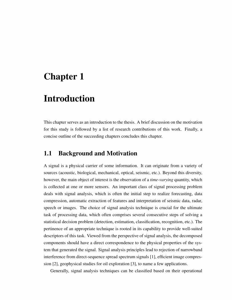
Figure 1.1: Time series representation of linear frequency modulated signal.
domain, namely, time, frequency or time-frequency, although in many cases these dis-
tinctions are merely implementational. The Fourier transform (FT) and its windowed
version, the short-time Fourier transform (STFT) are signal analysis techniques appli-
cable to signal components that are stationary or at least locally stationary. However,
signals in many practical situations, such as electroencephalogram (EEG) signals, which
are monitored to observe brain health, and speech signals are known to be nonstationary.
More advanced techniques utilizing localized unit energy elementary functions (called
time-frequency atoms) such as wavelets and chirplets have simple algorithmic structures
and seem to address the problems associated with nonstationary signals [2]. However,
optimum signal analysis using these techniques requires some a priori knowledge of
signal components.
There has been widespread agreement in the signal processing community over the
steps that constitute a general signal analysis procedure [4]:
1. Determine if the signal is stationary or not, and whether the signal is monocom-
ponent or multicomponent,
2. Break down the multicomponent signal into its subcomponents (usually using
3
time
freq
uenc
y
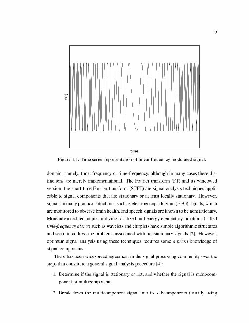
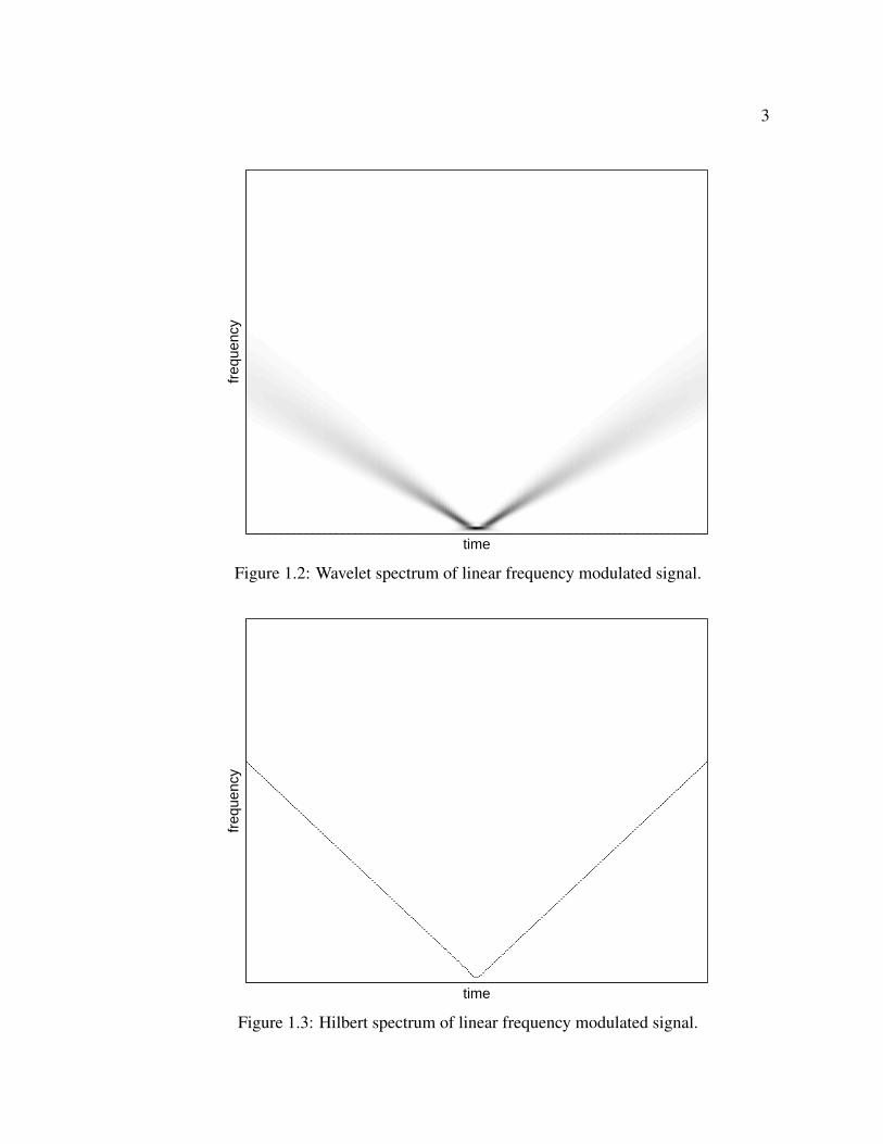
Figure 1.2: Wavelet spectrum of linear frequency modulated signal.
time
freq
uenc
y
Figure 1.3: Hilbert spectrum of linear frequency modulated signal.

4
time
freq
uenc
y
Figure 1.4: Result of direct application of Hilbert transform to multicomponent signal.The horizontal lines indicate the frequencies of the component tones. The time seriesdata is shown later in Fig. 2.3a.
windowing methods in the time-frequency domain),
3. Track the spectral variation of the components and indicate the energy concentra-
tion of the signal around its instantaneous frequency,
4. Model the signal. If each component of a multicomponent signal is defined in
terms of its amplitude and phase, then the analysis problem is to find these param-
eters for each of the signal components.
An accepted method of decomposing multicomponent signals with nonstationary com-
ponents is via time-frequency processing techniques involving wavelets and chirplets
amongst others.
1.1.1 Hilbert Spectrum of Simple Signals
An accurate and unambiguous frequency estimate of a sinusoidal signal is obtainable
using the FT. The FT possesses several desirable qualities such as ease of computation

5
time
freq
uenc
y
s(t)
time
freq
uenc
y
s1(t)
time
freq
uenc
y
s2(t)
time
freq
uenc
y
s3(t)
Figure 1.5: Time-frequency representation of three-component signal used to testwavelet decomposition and empirical mode decomposition (EMD). Top left panel showsthe time-frequency representation for the multicomponent signal. The remaining panelsshow individual components. The time-series for this example is shown in Fig. 3.14
and invertibility for stationary signals (signals whose frequency content do not change
with time). However, due to lack of time resolution, it is not invertible for nonstationary
signals (signals with time-varying frequency content). The STFT gains time resolu-
tion by performing FT on small data segments sequentially, thereby sacrificing some
amount of frequency resolution. This trade-off between time and frequency resolutions
is no accident, but a manifestation of the Heisenberg Uncertainty Principle. The wavelet
transform adaptively adjusts to the Heisenberg Uncertainty Principle by delivering good
resolution in time for large frequencies, and in frequency for small frequencies.
Analogous to the concept of frequency for stationary signals, the notion of instan-
taneous frequency of a nonstationary signal follows naturally. This quantity, which is
formally defined in Chapter 2, refers to the the number of oscillations per unit time as a
function of time for a signal. The Hilbert transform presents a practical way to compute
the instantaneous frequency of a signal. A two-dimensional representation of the instan-

6
time
freq
uenc
y
Figure 1.6: Hilbert spectrum of the result of wavelet decomposition of multicomponentsignal. Input is a three-component signal shown in Fig. 1.5.
taneous frequency, with time along the horizontal axis, and frequency along the vertical
axis is called the Hilbert spectrum. Compared to other time-frequency spectrums such
as the wavelet spectrum, the excellent time-frequency properties of the Hilbert spectrum
makes it a useful tool in the field of time-frequency analysis.
The time-frequency localization quality of the Hilbert and wavelet spectrums is
demonstrated next via an example. Consider a linear frequency modulated signal s(t).
This refers to a sinusoid with linearly-varying frequency. The time-domain signal is
shown in Fig. 1.1. The wavelet and Hilbert spectrums are shown in Figs. 1.2 and 1.3
respectively. The drawbacks of the wavelet spectrum are evident: poor frequency reso-
lution for large frequencies and poor time resolution for small frequencies. The Hilbert
spectrum, on the other hand, exhibits uniformly good time-frequency localization.
1.1.2 Hilbert Spectrum of Combination of Signals
We saw above that the Hilbert spectrum exhibits good time-frequency resolution for
simple signals called monocomponent signals, which refers to signals that have only one

7
time
freq
uenc
y
Figure 1.7: Result of application of Hilbert transform to EMD components. Input is athree-component signal shown in Fig. 1.5.
oscillatory mode at any time instant. However, this technique fails to provide meaningful
time-frequency representation for more complex signals, called multicomponent signals.
The example in Fig. 1.4 shows a multicomponent signal consisting of two tones and its
Hilbert spectrum. Since the Hilbert spectrum is meaningful only for monocomponent
signals, it fails to correctly identify the instantaneous frequencies of multicomponent
signal constituents in this example.
To obtain a meaningful value of instantaneous frequency using Hilbert transform
the multicomponent signal should be decomposed into its constituents before apply-
ing Hilbert transform on each component. The superposition of the individual Hilbert
spectrums gives the spectrum for the multicomponent signal. Any model-based non-
adaptive decomposition procedure will be ineffective in separating the signal compo-
nents, in general, due to fixed frequency boundaries. The empirical mode decomposi-
tion (EMD) technique, on the other hand, is fully data-driven, not model-based whose
purpose is to adaptively decompose any signal into its oscillatory contributions. There-
fore the resulting components admit meaningful instantaneous frequencies after Hilbert

8
transform. This concept is explained using an example. Consider a multicomponent
signal with three components as shown in Fig. 1.5. The analyzed signal is the sum of
two sinusoid frequency modulated components and a Gaussian wavepacket. The time-
frequency analysis of the multicomponent signal (top left panel in the figure) reveals
three time-frequency signatures that overlap in both time and frequency, thus forbidding
the components to be separated by any nonadaptive filtering technique. The instanta-
neous frequencies derived from wavelet decomposition and EMD are shown in Figs.
1.6 and 1.7 respectively. While the wavelet decomposition does not result in meaning-
ful instantaneous frequencies of the components, the EMD produces components with
the correct instantaneous frequencies. The time-domain signals for this example appear
later in Fig. 3.14.

9
1.2 Contributions of this Dissertation and Summary of
Publications
The following original contributions in signal analysis research are presented in this
dissertation:
1. Development of a new version of the EMD algorithm using raised cosine interpo-
lation with superior signal analysis properties (either more resolution or reduced
sampling requirements) and reduced computation requirement. This technique is
called raised cosine empirical mode decomposition (RCEMD).
2. Development of associated mathematical framework to study the signal analysis
performance of EMD-like algorithms for simple signals.
3. Introduction of an overlay communications technique using RCEMD technique
and its extension to covert communications.
4. Application of RCEMD technique for wideband interference rejection in wireless
communications.
5. Development of an RCEMD-based technique for study of persistent and sporadic
signal features in atmospheric pressure measurements using microbarographs with
higher precision than existing techniques.
6. Development of a signal analysis and parameter estimation estimation technique
for fragmenting radar meteor echoes using genetic algorithms.
Parts of this dissertation work appear in the following publications:
Book Chapter
1. A. Roy, and J. F. Doherty, “Nyquist Pulse based Empirical Mode Decomposition
and its Applications to Remote Sensing Problems,” in Signal and Image Process-
ing for Remote Sensing, 2nd Edition, CRC Press, to appear in 2011.
10
Journal Publications
1. A. Roy, and J. F. Doherty, “Raised cosine filter-based empirical mode decompo-
sition,” IET Signal Processing, vol. 5, no. 2, pp. 121-129, Apr. 2011.
2. A. Roy, and J. F. Doherty, “Overlay communications using empirical mode de-
composition,” IEEE Systems Journal, vol. 5, no. 1, pp. 121-128, Mar. 2011.
3. A. Roy, and J. F. Doherty, “Covert communications using signal overlay,” Ad-
vances in Adaptive Data Analysis, vol. 2, no. 3, pp. 295-311, 2010.
4. A. Roy, and J. F. Doherty, “Improved signal analysis performance at low sampling
rates using raised cosine empirical mode decomposition,” Electronic Letters, vol.
46, no. 2, pp. 176-177, Jan. 2010.
5. A. Roy, S.J. Briczinski, J.F. Doherty, and J. D. Mathews, “Genetic algorithm
based parameter estimation technique for fragmenting meteor head-echoes,” IEEE
Geoscience and Remote Sensing Letters, vol. 6, no. 3, pp. 363-367 July 2009.
6. A. Roy, C.-H. Wen, J. F. Doherty, and J. D. Mathews, “Signal feature extraction
from microbarograph observations using the Hilbert-Huang transform (HHT),”
IEEE Transactions on Geoscience and Remote Sensing, vol. 46, no. 5, pp. 1442-
1447, May 2008.
Conference Proceedings
1. A. Roy, and J. F. Doherty, “Partial band jamming excision in WCDMA using
raised cosine empirical mode decomposition,” in Proc. Wireless @ Virginia Tech
2010 Symposium and Summer School, Blacksburg, VA, 2-4 Jun. 2010.
2. A. Roy, and J. F. Doherty, “Covert communications using empirical mode de-
composition,” in Proc. 2009 IEEE Sarnoff Symposium, Princeton, NJ, pp. 1-5, 30
Mar.-1 Apr. 2009.
3. A. Roy, and J. F. Doherty, “Raised cosine interpolation for empirical mode de-
composition,” in Proc. 43rd Annual Conference on Information Sciences and
Systems, 2009, CISS 2009, Baltimore, MD, pp. 888-892, 18-20 Mar. 2009.
11
4. A. Roy, and J. F. Doherty, “Empirical mode decomposition frequency resolution
improvement using the pre-emphasis and de-emphasis method,” in Proc. 42nd An-
nual Conference on Information Sciences and Systems,2008, CISS 2008, Prince-
ton, NJ, pp. 453-457, 19-21 Mar. 2008.
1.3 Dissertation Outline
This dissertation consists of two independent, yet related parts. The theoretical part
of this dissertation comprising Chapters 3 through 6 involves introduction of a new
signal analysis algorithm related to EMD followed by development of new applications
and performance verification based on mathematical models. The next part, covering
Chapters 7 and 8, describes remote sensing applications of signal analysis techniques
using in-field measurements.
Part I of this dissertation introduces a new signal analysis algorithm related to EMD
that uses raised cosine interpolation called RCEMD. Theoretical development of this
technique, development of mathematical tools to formalize the study of EMD perfor-
mance, performance comparison of the two algorithms, and development of communi-
cations applications based on RCEMD including signal overlay, covert communications,
and interference cancelation from spread spectrum signals are covered in this part.
Chapter 2 introduces signal analysis concepts and techniques from a historical
perspective. Techniques such as FT, STFT, wavelet decomposition and EMD are
discussed. The EMD technique is described in some detail along with some al-
gorithmic variations and applications. The chapter also includes a discussion on
select time-frequency concepts that are used in later chapters.
Chapter 3 introduces the RCEMD technique for signal analysis. In addition to
algorithmic description of this new technique, a generalized mathematical frame-
work is developed to study the performance of iterative signal analysis algorithms
following the basic idea of EMD. Advantages of this new technique related to
improved frequency resolution, relaxed sampling requirements and fewer com-
putations are demonstrated using a combination of synthetically-generated and
real-life signals.

12
Chapter 4 describes the pre-emphasis and de-emphasis technique to enhance the
signal analysis quality of iterative algorithms like EMD. Improved frequency res-
olution for a specific configuration of constituent signal components is demon-
strated using synthetic signal examples. Further, the effect of certain algorithmic
parameters on signal analysis performance is demonstrated.
Chapter 5 presents a new signal overlay technique using RCEMD. This technique
frequency spectrum utilization for wireless communications by enabling oppor-
tunistic communications by a secondary user on the same frequencies as an ex-
isting primary user. Feasibility of this technique is demonstrated using computer
simulations based on mathematical models of wireless channels and transceivers.
A covert version of this technique using frequency-hopping (FH) technique is also
described.
Chapter 6 describes a new application of RCEMD to wideband interference sup-
pression in wireless communications. Here, the problem of nonstationary interfer-
ence affecting a widely used communication standard is considered and a solution
based on RCEMD is formulated. Simulation study results analyzing the effective-
ness of the technique are presented.
Part II of this dissertation introduces new signal processing techniques for remote sens-
ing applications. This includes development of periodic and sporadic feature isolation
techniques using the RCEMD procedure developed in Part I for microbarograph ob-
servations, and a genetic algorithm based technique for accurate meteoroid fragment
parameter estimation based on radar meteor head-echoes.
Chapter 7 describes a novel feature extraction procedure using RCEMD applied
to data recorded using sensors deployed to measure atmospheric pressure. The
ability to isolate hurricane signature and extract diurnal and semi-diurnal atmo-
spheric tide signals from the noisy raw data with greater precision than existing
techniques is demonstrated.
Chapter 8 introduces a new method to study meteoroid fragmentation using ge-
netic algorithms to radar measurements. Radar returns from multiple, closely-
spaced traveling particles result in an interference pattern, rendering signal anal-
ysis necessary for study of individual particle behavior. A method using genetic

13
algorithms is developed to estimate orbital parameters of such fragmenting mete-
oroids in this chapter.
Chapter 9 discusses the important findings and results of this work and highlights
some relevant open problems.
Chapter 2
Time-Frequency Analysis of Signals
This chapter provides a brief presentation of the basic concepts related to time-frequency
analysis of signals. It begins with a review of important time-frequency concepts such
as analytic signals, monocomponent and multicomponent signals and instantaneous fre-
quency. Next, various tools available to analyze a nonstationary signal are studied and
their relative merits are compared. This is followed by a description of the EMD algo-
rithm for signal analysis. Finally, an overview of the the developments in the field of
EMD and its applications concludes this chapter.
2.1 Signal Analysis: Concepts
In this section some basic concepts related to time-frequency analysis of signals are
presented. We start by defining an analytical signal, then move on to instantaneous
frequency of a signal, and finally discuss the classification of signals as monocomponent
and multicomponent.
2.1.1 Analytical Signal
The phase of a signal may be required in some cases, for example to determine its
instantaneous frequency, a concept that will discussed in Section 2.1.2. Thus, a proper
definition of the phase is required. To properly define the phase ϕ(t) for a real signal
f (t), Gabor [5] proposed an approach to “suppress the amplitudes belonging to negative
frequencies and multiply the amplitudes of positive frequencies by two.” Following this
15
approach, the Gabor’s time domain complex signal can be defined as follows
z(t) = 21√2π
∞∫0
F(ω)eıωtdt (2.1)
where
F(ω) =1√2π
∞∫−∞
f (t)e−ıωtdt. (2.2)
This yields
z(t) = f (t)+iπ
P∞∫
−∞
f (τ)t − τ
dτ, (2.3)
where P∫
denotes the principal value integral defined as [6]
P
β∫α
f (u)du = limε→0+
ξ−ε∫α
f (u)du+
β∫ξ+ε
f (u)du
. (2.4)
This class of complex functions satisfy the Cauchy-Riemann conditions for differentia-
tion and are called analytic functions [7, 8] and thus z(t) is called analytical signal [9].
2.1.2 Instantaneous Frequency
The frequency of a stationary signal is well-defined following the Fourier approach.
Generally, the frequency is defined as the number of oscillations per unit time of a
physical field parameter such as displacement, current or electromagnetic waves. But
for nonstationary signals commonly encountered in radar, seismic and communications
applications this definition becomes ambiguous [9] due to the time-varying nature of the
spectral characteristics of the signal. This leads to the notion of instantaneous frequency
of a signal. Gabor [5] was the first to introduce a complex analytic signal, which was
later employed to define instantaneous frequency as the time derivative of the phase of a
signal by Ville [10]. This definition works well for monocomponent signals. However,
it fails to produce physically reasonable results for multicomponent signals. Cohen [11]
also used the concept of instantaneous frequency, as well as instantaneous bandwidth to
explain what a multicomponent signal is. He defined the instantaneous frequency of a
16
monocomponent signal as an average of the frequencies that exist at a particular time,
and the instantaneous bandwidth as the spread of the frequencies about the average for
that time.
For a mathematical definition we reconsider (2.3) where the imaginary part is the
Hilbert transform f (t) of the signal f (t) [12]. Then (2.3) can be written as
z(t) = f (t)+ f (t) (2.5)
or in the exponential form
z(t) = a(t)eıϕ(t), (2.6)
where amplitude a(t), and the phase ϕ(t) are defined as
a(t) =√
f 2(t)+ f 2(t), and ϕ(t) = arctanf (t)f (t)
(2.7)
respectively. Therefore, the instantaneous frequency of the signal x(t) is
IF(t) =dϕ(t)
dt=
f (t) ˙f (t)− f (t) f (t)f 2(t)− f 2(t)
. (2.8)
The above definition captures the notion of instantaneousness in nature and fits our
intuitive expectation of the instantaneous frequency concept. It is encouraging that when
the definition is applied to a sinusoidal signal, the obtained instantaneous frequency is
exactly the frequency of the signal.
2.1.3 Monocomponent and Multicomponent Signals
Although several definitions of a multicomponent signal exist in literature, the one pro-
posed by Boashash [4] is the most widely accepted and therefore adopted in this work.
Accordingly, an analytical signal is referred to as a monocomponent signal if its instan-
taneous frequency accurately represents the frequency modulation of the signal, and if
the signal is single-valued and invertible (so that the inverse function of the instanta-
neous frequency exists). An asymptotic signal z(t) is referred to as multicomponent if
there exists a finite number N of monocomponent signals zi(t), i = 1, 2, ...,N, such that
the relation z(t) =N∑
i=1zi(t) holds for all values of t for which z(t) is defined, and this
17
decomposition is meaningful.
2.2 Signal Analysis: Methods
In studying time series, several methods have been developed and used by researchers
and practitioners. The ones that are frequently used include FT, STFT, wavelet trans-
form, Wigner-Ville representation, adaptive chirplet decomposition and EMD (which is
a part of the Hilbert-Huang transform). In the following, basic information about these
methods is presented. Each method has its own advantages and disadvantages depend-
ing on the application at hand.
2.2.1 Fourier Analysis
The most commonly used method has been Fourier analysis. It reveals the frequency
content of a signal by decomposing it into sinusoids of different frequencies. Fourier
series is used for periodic signals, whereas for nonperiodic signals there is FT.
2.2.1.1 Fourier Series
Fourier stated that any periodic signal f (t) of period T (i.e., f (t) = f (t + T )) can be
expressed as
f (t) =a0
2+
∞
∑k=1
akcos(kω0t)+∞
∑k=1
bksin(kω0t) (2.9)
where ω0 =2πT is the fundamental angular frequency in radians per second. The coeffi-
cients of the sine and cosine terms (Fourier coefficients) are obtained as follows:
a0 =2T
T/2∫−T/2
f (t)dt
ak =2T
T/2∫−T/2
f (t)cos(kω0t)dt (2.10)
bk =2T
T/2∫−T/2
f (t)sin(kω0t)dt, k = 1, 2, ..., ∞.

18
2.2.1.2 Fourier Transform
While FT of a square integrable function f ( f ∈ L2(RRR)) 1 has already been defined (2.2),
its inverse can be written as follows
f (t) =1√2π
∞∫−∞
F(ω)eıωt . (2.11)
Analyzing signals by FT, called spectral analysis, is a standard technique to obtain
information about a periodic signal. The discrete Fourier transform (DFT) extends the
use of FT to sampled time series data. DFT can be computed in a fast way using an
algorithm called the butterfly algorithm [13] that computes the coefficients recursively.
While FT gives valuable information about frequencies in a seismogram, it is not
possible to have any information on temporal location of those frequencies. Therefore,
it is suitable only for stationary signals. To overcome this problem STFT was proposed.
2.2.2 Short-Time Fourier Transform
The idea behind STFT is to cut the original signal into segments of smaller duration
and applying FT to obtain the frequency components of each slice. The functions ob-
tained by this crude slicing are not periodic in general and FT will interpret the jumps
at the boundaries as discontinuities and will introduce higher order harmonics to fit the
waveform. To avoid these, the concept of windowing has been introduced. Instead of
localizing by means of rectangular function, a smooth window function, which is close
to unity near origin and decays towards zero at the edges, is used. For this reason STFT
is sometimes called windowed FT. Any square integrable function may be used as a
window, but certain criteria should be met for good performance. The main property of
a good window is its good localization in both time and frequency domains. Some win-
dows are favorable such as Hamming, Hanning, Bartlett, Blackman, Kaiser, Gaussian2 [14], and the discrete prolate spheroid [15]. The reason for the use of these windows is
that they have functional forms and their FT is concentrated around ω = 0. The window
1In mathematics, a square integrable function is a real- or complex-valued measurable function for
which the integral of the square of the absolute value is finite, i.e.,∞∫
−∞| f (x)|2dx < ∞.
2Note that STFT using Gaussian window has the special name Gabor transform, and is known tooptimize the Heisenberg’s uncertainty principle.

19
in the time-domain is referred to as the time window and its FT as the spectral window.
The signal is multiplied by one of the window functions g(t −b), where g(t) repre-
sents the functional form of the window and is nonzero only in a finite region around
time b. Then the FT of f (t)g(t − b) is taken, and the window is moved to a different
location to repeat the operation. The method can therefore be represented by
S f (ω ,b) =1√2π
∞∫−∞
f (t)g(t −b)e−iωtdt. (2.12)
The signal can be reconstructed from its transform by the formula
f (t) =1√2π
∞∫−∞
∞∫−∞
S f (ω ,b)g(t −b)eiωt . (2.13)
The fundamental problem with STFT is that it has fixed resolution along both time
and frequency axes. As argued by Chui [16], since frequency is directly proportional to
number of cycles in a specific time interval, a narrow time window is required to locate
high-frequency phenomena and a wide time-window is necessary for more thorough
investigation of low frequency phenomena. As a result, the STFT is not well suited for
analysis of signals that may have both low and high frequency components.
2.2.3 Wavelet Transform
Wavelet analysis has emerged as a powerful tool to analyze a signal with particular
effectiveness for nonstationary signals. A wavelet is a small wave with finite energy,
which has its energy concentrated in time or frequency to serve as a “basis function” for
the analysis of transient phenomena. While being similar to Fourier analysis as far as
complex expansions are concerned, it differs by decomposing a signal into a series of
local basis functions called wavelets. Each wavelet is located at a different position of
the time axis and is local in the sense that it decays to zero away from its center. The
terminology “wavelet” was first introduced, in the context of a mathematical transform
by Grossmann and Morlet [17]. The wavelet transform is a two-parameter expansion
of a signal in terms of a particular wavelet basis function or mother wavelet. Temporal
analysis is performed with a contracted high frequency version of the prototype wavelet,
20
while frequency analysis is performed with a dilated, low frequency version of the same
wavelet.
2.2.3.1 Continuous Wavelet Transform (CWT)
In spite of its name, the continuous wavelet transform (CWT) is a discrete process in
implementation. Its continuity comes from the flexibility of the set of scales and posi-
tions on which it operates. Unlike the discrete wavelet transform the CWT can operate
at every scale. The CWT is also continuous in terms of shifting: during computation,
the analyzing wavelet is shifted smoothly over the full domain of the analyzed function.
Let ψ(t) be the mother wavelet. All other wavelets are obtained by scaling and
translating ψ(t) as follows [18]:
ψa,b =1√a
ψ(
t −ba
). (2.14)
Let f (t) be a square integral function of time t. The CWT of f (t) is defined as
Wψ fa,b =
∞∫−∞
f (t)ψ∗a,b(t)dt =
1√a
∞∫−∞
f (t)ψ∗(
t −ba
)dt (2.15)
where a, b ∈ R, a = 0 and .∗ denotes complex conjugate. The normalizing factor 1√a
is used to keep the energy level the same for different values of a and b. In CWT
nomenclature a is called scale parameter and b is called translation parameter. When a
is increased the wavelet ψa,b(t) is dilated and when b is varied, the signal is translated in
time. After the parameters a and b are selected, the basis or mother wavelet is stretched
or dilated according to the as and translated according to the bs to produce a family of
wavelets ψa,b(t). The wavelets ψa,b(t) are multiplied by f (t) at different scales and dif-
ferent translations. The CWT coefficients are obtained by summing the product showing
the correlation between the signal and the wavelet functions. The original time domain
signal can be reconstructed through the inverse wavelet transform
f (t) =1
2πCψ
∞∫−∞
∞∫−∞
Wψ fa,b
a2 ψa,b(t)dadb (2.16)

21
where
Cψ =
∞∫−∞
|ψ(ω)|2
|ω|dω (2.17)
and ψ(ω) is the FT of ψ(t).
A wavelet analysis is often called a time-scale analysis rather than a time-frequency
analysis because the analysis function ψ(t) is scaled by a. Among these wavelets are or-
thogonal, biorthogonal and harmonic wavelet systems. Orthogonal wavelets decompose
signals into well-behaved orthogonal signal spaces. In 1988, Daubechies introduced
a class of compactly-supported orthogonal wavelets with growing smoothness for in-
creasing support. Mallat [19] and Meyer [20] presented the theory of multiresolution
analysis.
2.2.3.2 Discrete Wavelet Transform (DWT)
The discrete wavelet transform (DWT) is more efficient in terms of computational ef-
fort than CWT because of the dyadic nature of the scales and positions. In contrast to
CWT that uses a flexible frequency range, DWT uses frequency only in the octave band.
Although this later method is computationally less expensive, it does not give a very
precise result to interpret, and is used mostly in signal compression.
Let f [n] be the discrete signal obtained by a low-pass filtering of a continuous time
signal and uniform sampling at intervals N−1. Its DWT can only be calculated at scales
N−1 < s < 1. It is calculated for s = a j, with a = 21/v, which provides v intermediate
scales in each octave [2 j,2 j+1).
Let ψ(t) be a wavelet with a support included in [−K/2,K/2]. For 1 ≤ a j ≤ NK−1,
a discrete wavelet scaled by a j is defined by
ψ j[n] =1√a j
ψ( n
a j
). (2.18)
To avoid border problems we treat f [n] and the wavelets ψ j[n] as periodic signals of
period N. The discrete wavelet transform can then be written as a circular convolution
with ψ j[n] = ψ∗j [−n] [21]:
W f [n,a j] =N−1
∑m=0
f [m]ψ∗j [m−n] = f ~ ψ j[n]. (2.19)

22
This circular convolution is calculated with the fast Fourier transform algorithm that
requires O(Nlog2N) operations.
An advantage of the wavelet transform is that although there are numerous time-
frequency transformations available, the wavelet transform is uniquely capable of adap-
tively adjusting to the Heisenberg’s uncertainty principle. In essence, the wavelet trans-
form concedes that arbitrarily good resolution in both time and frequency is impossible.
Thus, the transform optimizes its resolution as needed. It provides good resolution at
high dilations or low frequencies, while sacrificing time resolution to satisfy the uncer-
tainty principle. In the time domain, the transform has good resolution at high frequen-
cies in order to identify signal singularities or discontinuities.
A major disadvantage of wavelet transform, as compared to EMD, is that its perfor-
mance depends upon the choice of mother wavelet. Although there are wavelets that
have good time or frequency resolution, there is no wavelet that has uniformly superior
performance for all applications. The choice of mother wavelet depends on a priori
knowledge of the frequency content of signal to be analyzed.
2.3 Bilinear Time-Frequency Distribution
The STFT and CWT are based on the concept of finding the similarity between the sig-
nal and the analyzing functions and have the disadvantage that Heisenberg’s uncertainty
principle restrains their time-frequency resolution. Another approach which in several
cases gives significantly better results is the bilinear (quadratic) time-frequency analysis
by means of time-frequency distributions. A comprehensive review [22] provides an
overview of time-frequency distributions. This section addresses a specific subset of t-f
distributions belonging to Cohen’s class. These are the time-shift and frequency-shift
invariant t-f distributions. For these distributions, a time shift in the signal is reflected as
an equivalent time shift in the t-f distribution, and a shift in the frequency of the signal
is reflected as an equivalent frequency shift in the t-f distribution. The spectrogram, the
Wigner-Ville distribution (WVD) and the reduced interference distributions (RID) all
have this property. Different distributions can be obtained by selecting different ker-
nel functions in the Cohen’s class. Performance comparison of several time-frequency
distributions in terms of resolution is provided in [4].

23
2.3.1 The Wigner-Ville Distribution
The WVD has been employed as an alternative to overcome the liabilities and limitations
of the spectrogram. It was first introduced in the context of quantum mechanics [23] and
revived for signal analysis by Ville [10]. It provides a high-resolution representation in
time and in frequency for a nonstationary signal such as chirp. In addition, WVD has
the important property of satisfying the time and frequency marginals in terms of the
instantaneous power in time and energy spectrum in frequency. However, its energy
distribution is not nonnegative and it often possesses severe cross-terms, or interference
terms, between components in different t-f regions, potentially leading to confusion and
misinterpretation.
The WVD of real signal f (t) is defined as
Wz(t,ω) =
∞∫−∞
z(
t +τ2
)z∗(
t − τ2
)e− jωτdτ (2.20)
where z(t) is the analytic “associate” of f (t) (see Section 2.1.1). This process is the
correlation of the signal with itself. We may interpret this equation as the computation
of a “local” autocorrelation function at each time instant, t, followed by the evaluation
of its Fourier transform. This leads to a “local” power spectral density at each time
instant. In practice, only one realization of the process is available and this forces us to
ignore the implicit expectation operation in autocorrelation. The Wigner-Ville transform
is optimally localized in the time domain for Dirac signals, and in the frequency domain
for linear chirps.
Equation 2.20 defines time-frequency distributions that are quadratic (bilinear) in the
signal z(t). This implies that if z(t) consists of two components z1(t) and z2(t), then the
quadratic time-frequency representation will not only include the two components but
also their cross product z1(t)z2(t). The extra terms are known as cross-terms, or artifacts
and they are a major drawback of multicomponent signal time-frequency analysis using
quadratic time-frequency distributions. It can be shown that the WVD of the signal
z(t) = z1(t)+ z2(t) is given by
Wz1(t)+z2(t)(t,ω) =Wz1(t)(t,ω)+Wz2(t) (2.21)

24
+2Re
∞∫
−∞
z1
(t +
τ2
)z∗2(
t − τ2
)e− jωτdτ
(2.22)
The last term in this expression is the cross-term. The cross-terms in the WVD are
oscillating contributions located midway between the components. Note that for a mul-
ticomponent signal with N components, there will be N(N − 1)/2 cross-terms in the
signal WVD. As the number of cross-terms increases quadratically their interpretation
becomes impossible. Although this cross-term interference is a good indication that the
signal is multicomponent, it reduces the resolution of the WVD and thus is in general
undesirable.
2.3.2 Reduced Interference Distributions
In order to suppress the cross-terms in the WVD of multicomponent signals, the WVD
can be convolved with a smoothing function g(t,ω) which is commonly referred to as
kernel. That is,
Cz(t,ω) =Wz(t,ω)⊗g(t,ω) (2.23)
where the symbol ⊗ denotes two-dimensional convolution. The set of all bilinear distri-
butions of 2.23 is called Cohen’s class.
With this general approach an infinite number of time-frequency representations can
be generated by appropriately selecting a kernel g(τ,θ). Obviously, the kernel for WVD
is
gWV D(τ,θ) = 1. (2.24)
Then the Cohen’s class distributions for a kernel g(τ,θ) can be written as
Cz(t,ω) =1
4π2
∞∫−∞
∞∫−∞
A(τ,θ)G(τ,θ)e− j(τt+θω)dτdθ , (2.25)
where G(τ,θ) is the Fourier transform of the kernel g(t,ω) and A(τ,θ) is the symmet-
rical ambiguity function defined as the Fourier transform of the WVD
A(τ,θ) =∞∫
−∞
z(
t +τ2
)z∗(
t − τ2
)e− jθτdτ. (2.26)

25
These distributions are also called reduced interference distributions (RIDs). One
of the first RIDs was the Choi-Williams distribution (CWD). Choi and Williams [24]
defined a two-dimensional Gaussian-shaped kernel in Doppler-lag domain as:
g(θ ,τ) = e−(θτ)2/σ (2.27)
where σ is a smoothing parameter that controls the kernel spread in the ambiguity do-
main, and so controls the amount of cross-terms suppression in the time-frequency do-
main. The σ parameter may be varied over a range of values to obtain different trade-
offs between cross-term suppression and auto-term time-frequency resolution, since the
kernel, while reducing the cross-term, increases smearing in the time-frequency domain.
Large computational requirement is another serious drawback of this approach.
2.4 Time-Frequency Distribution Illustration
Before moving on to the EMD technique we study the performance of the different
spectral and time-frequency techniques considered here using two examples:
Example 1: Monocomponent signal
We again go back to the linear frequency modulated signal first studied in Chapter 1.
Figure 2.1 shows the Fourier spectrum, spectrogram, wavelet spectrum and the WVD
spectrum for the monocomponent signal. While no information about frequency varia-
tion of the signal is available from the Fourier transform, the other spectrums are suc-
cessful in conveying the time varying frequency of the signal to varying degrees. The
uniform resolution of the STFT (spectrogram) has been mentioned before. Moreover,
this example clearly shows the variable frequency resolution of the wavelet spectrum.
Finally, the excellent resolution of the WVD is not surprising due to its optimality for
linear frequency modulated signals.
Example 2: Multicomponent signal
Here we consider a multicomponent signal consisting of two linearly frequency modu-
lated signals with intersecting frequencies. We show the corresponding spectral repre-
sentations in Fig. 2.1. This example represents a particularly difficult problem due to
26
frequency
ampl
itude
a.
time
freq
uenc
y
b.
time
freq
uenc
y
c.
time
freq
uenc
y
d.
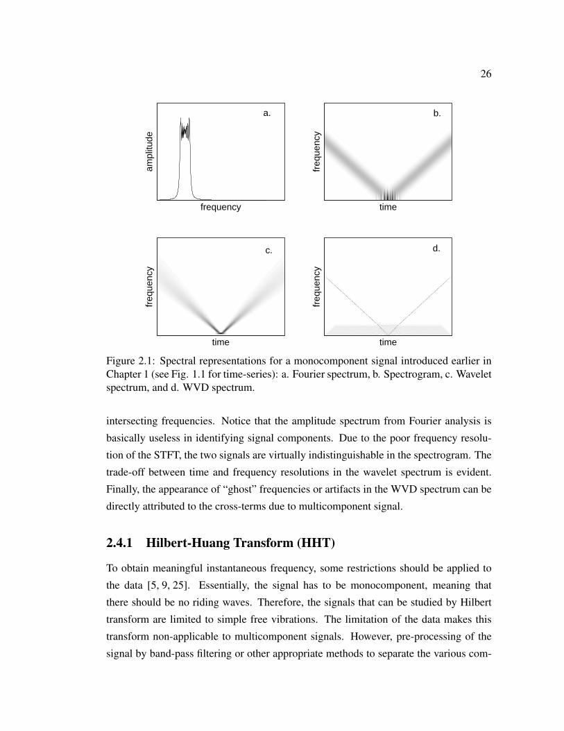
Figure 2.1: Spectral representations for a monocomponent signal introduced earlier inChapter 1 (see Fig. 1.1 for time-series): a. Fourier spectrum, b. Spectrogram, c. Waveletspectrum, and d. WVD spectrum.
intersecting frequencies. Notice that the amplitude spectrum from Fourier analysis is
basically useless in identifying signal components. Due to the poor frequency resolu-
tion of the STFT, the two signals are virtually indistinguishable in the spectrogram. The
trade-off between time and frequency resolutions in the wavelet spectrum is evident.
Finally, the appearance of “ghost” frequencies or artifacts in the WVD spectrum can be
directly attributed to the cross-terms due to multicomponent signal.
2.4.1 Hilbert-Huang Transform (HHT)
To obtain meaningful instantaneous frequency, some restrictions should be applied to
the data [5, 9, 25]. Essentially, the signal has to be monocomponent, meaning that
there should be no riding waves. Therefore, the signals that can be studied by Hilbert
transform are limited to simple free vibrations. The limitation of the data makes this
transform non-applicable to multicomponent signals. However, pre-processing of the
signal by band-pass filtering or other appropriate methods to separate the various com-
27
frequency
ampl
itude
a.
time
freq
uenc
y
b.
time
freq
uenc
y
c.
time
freq
uenc
y
d.
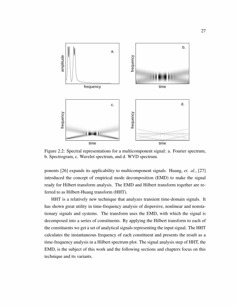
Figure 2.2: Spectral representations for a multicomponent signal: a. Fourier spectrum,b. Spectrogram, c. Wavelet spectrum, and d. WVD spectrum.
ponents [26] expands its applicability to multicomponent signals. Huang, et. al., [27]
introduced the concept of empirical mode decomposition (EMD) to make the signal
ready for Hilbert transform analysis. The EMD and Hilbert transform together are re-
ferred to as Hilbert-Huang transform (HHT).
HHT is a relatively new technique that analyzes transient time-domain signals. It
has shown great utility in time-frequency analysis of dispersive, nonlinear and nonsta-
tionary signals and systems. The transform uses the EMD, with which the signal is
decomposed into a series of constituents. By applying the Hilbert transform to each of
the constituents we get a set of analytical signals representing the input signal. The HHT
calculates the instantaneous frequency of each constituent and presents the result as a
time-frequency analysis in a Hilbert spectrum plot. The signal analysis step of HHT, the
EMD, is the subject of this work and the following sections and chapters focus on this
technique and its variants.

28
2.5 Empirical Mode Decomposition
The EMD is an adaptive signal-dependent decomposition with which any complicated
signal can be decomposed into a series of constituents. Adding all the extracted con-
stituents together reconstructs the original signal without information loss or distortion.
Many methods exist that analyze signals simultaneously in the time and frequency do-
mains, some of which were highlighted in Section 2.2. These methods are based on the
expansion of the signal into a set of basis functions that are defined by the method. The
concept of EMD is to expand the signal into a set of functions defined by the signal
itself. These decomposed constituents are called intrinsic mode functions (IMF). Signal
adaptive decomposition by means of Principal Component Analysis (PCA) [28] also
expands the signal into a basis defined by the signal itself. PCA differs from EMD in
that it is based on the signal statistics, while EMD is deterministic and is based on local
properties.
The EMD process allows time-frequency analysis of transient signals for which
Fourier based methods have been unsuccessful. Whenever we use the Fourier trans-
form to represent frequencies we are limited by the uncertainty principle. For infinite
signal length we can get exact information about the frequencies in the signal, but when
we restrict ourselves to analyze a signal of finite length there is a bound on the pre-
cision of the frequencies that we can detect. The instantaneous frequency represents
the frequency of the signal at one time, without any information of the signal at other
times. A problem with using instantaneous frequency is that it provides a single value
at each time. A multicomponent signal consists of many intrinsic frequencies and this
is where the EMD is used, to decompose the signal into its IMFs, each with its own
instantaneous frequency, so that multiple instantaneous frequencies of the signal com-
ponents can be computed. Another advantage of EMD is that it results in an adaptive
signal-dependent time-variant filtering procedure able to directly extract signal compo-
nents which significantly overlap in time and frequency [29]. Moreover, the physical
meaning of the intrinsic processes underlying the complex signal is often preserved in
the decomposed signals. This is mainly due to the fact that the results are not influenced
by predetermined bases and/or subband filtering processes.
EMD represents a totally different approach to signal analysis. EMD is an adap-
tive decomposition with which any complicated signal can be decomposed into a series
29
of constituents. EMD is an analysis method that in many respects gives a better un-
derstanding of the physics behind the signals. Because of its ability to describe short
time changes in frequencies that cannot be resolved by Fourier spectral analysis, it can
be used for nonlinear and nonstationary time series analysis. Each extracted signal ad-
mits well-defined instantaneous frequency. The original purpose for the EMD was to
find a decomposition that made it possible to use the instantaneous frequency for time-
frequency analysis of nonstationary signals. In the following sections we explore this
technique in more detail.
2.5.1 Procedure
As discussed above, the elementary AM-FM-type signal components that are produced
by the EMD procedure are called IMFs in literature. The original researchers outlined
two conditions that must be satisfied by an extracted component to be declared an IMF
[27]:
1. The number of extrema and the number of zero crossings must differ at most by
one.
2. The mean value of the envelopes defined by the local maxima and the local min-
ima should be zero at any point, meaning that the functions should be symmetric
with respect to the local zero mean.
Each of these IMFs is extracted by a process called sifting. The goal of sifting is
to remove the higher frequency components until only the low frequency components
remain. Given a signal x(t) the sifting procedure divides it into a high frequency detail,
d(t), and the low frequency residual (or trend), m(t), so that x(t) = m(t)+ d(t). This
detail becomes the first IMF and the sifting process is repeated on the residual, m(t) =
x(t)−d(t). After K iterations of the sifting procedure the input signal can be represented
as follows
x(t) =K
∑k=1
yk(t)+mK(t) (2.28)
where yk(t), k = 1, ...,K represent the IMFs and mK(t) is the residual, or the mean
trend, after K sifting iterations. The effective algorithm of EMD can be summarized as
follows [29]:

30
1. Identify all extrema of x(t).
2. Interpolate between minima (respectively maxima), resulting in the envelope emin(t)
(respectively emax(t)).
3. Compute the mean m(t) = (emin(t)+ emax(t))/2.
4. Extract the detail d(t) = x(t)−m(t).
5. If d(t) satisfies all IMF conditions, then set y1(t) = d(t), the first IMF, else repeat
above steps with d(t).
6. Evaluate the residual m1(t) = x(t)− y1(t).
7. Iterate on the residual m1(t).
Steps 1 through 4 may have to be repeated several times until the detail d(t) satisfies
the IMF conditions. Practical methods to determine if d(t) satisfies the IMF conditions,
also called stopping criteria, are discussed next. In the original work [27] the sifting
procedure for a particular IMF stops when the normalized difference in the extracted
signal between two consecutive iterations is smaller than a pre-determined threshold
ε . A new stopping criterion was suggested in [30] where the iterations stop when the
envelope mean signal is close enough to zero (|m(t)|< ε, ∀t). The reason for this choice
is that forcing the envelope mean to zero will guarantee the symmetry of the envelope
and the correct relation between the number of zero crossings and number of extremes
that define the IMF. A modified version of this stopping criterion with two thresholds
was introduced in [29], along with a discussion of typical threshold values. Yet another
stopping criterion was introduced in [31] where sifting is stopped when the number
of extrema and zeros crossings remains constant over some pre-determined number of
iterations. The latter is the most commonly used criterion. An example is presented next
to show the algorithmic steps pictorially.
Example: Decomposition of Tones
The EMD algorithm is demonstrated pictorially using a simple combination of tones of
the form
x(t) = s1(t)+ s2(t) (2.29)

31
where the two tones are
s1(t) = A1cos(2π f1t +ϕ1),
s2(t) = A2cos(2π f2t +ϕ2) (2.30)
and the symbols have their usual meanings with f1 > f2. Intermediate signals generated
by the algorithm are shown in Fig. 2.3.
Fig. 2.3a shows the original signal followed by the positions of the positive and
negative extrema (also called maxima and minima) in Fig. 2.3b. Smooth envelopes
are drawn through the identified maxima and minima using cubic spline interpolation.
These curves, denoted by emax(t) and emin(t) in the algorithm listed above, are shown
in Fig. 2.3c along with their mean, m(t). We omit the original signal in this figure for
clarity. The mean of the two envelopes, represented by the dashed curve, is a slowly-
varying signal that resembles the smaller tone, s1(t). The mean signal and the detail,
d(t), obtained by subtracting the mean from the original signal are shown in the two
panels of Fig. 2.3d, superimposed on the two tones, s2(t) and s1(t), respectively. The
resemblance between the mean and the detail signals and the original tones is obvious at
this stage. The process of computing the envelopes, mean and detail signals continues
by iterating on the detail signal. The result after five iterations, shown in Fig. 2.3e
indicates good decomposition quality
2.5.2 Algorithmic Variations
Several variations of the original algorithm have been proposed by researchers either to
improve the performance or to simplify the implementation. Some of the ways by which
the algorithm has been modified include different interpolation methods, new ways of
identifying IMFs, extending the algorithm to two dimensions and optimization-based
decomposition. We discuss some of these modifications here.
In order to construct smooth envelopes through the respective extrema, on each
subinterval x(t), tk ≤ t ≤ tk+1, where the kth and k+1th extrema are located at tk, tk+1,
an interpolant to the given values and certain slopes at the two end points is devised.
Between any two neighboring end-points x(tk) and x(tk+1), x(t) is a polynomial. Neigh-
boring polynomials match in value, and derivatives across their common end-points.
The interpolation to produce envelopes from the extrema points can be performed in dif-

32
0 0.5 1 1.5 2 2.5 3−2
−1.5
−1
−0.5
0
0.5
1
1.5
2
x(t) = s1(t) + s
2(t)
(a)
0 0.5 1 1.5 2 2.5 3−2
−1.5
−1
−0.5
0
0.5
1
1.5
2Positive and negative extrema
(b)
Figure 2.3

33
0 0.5 1 1.5 2 2.5 3−2
−1.5
−1
−0.5
0
0.5
1
1.5
2
emin
, emax
and m(t)
(c)
0 0.5 1 1.5 2 2.5 3−1.5
−1
−0.5
0
0.5
1
1.5
IMF1 and s1(t)
0 0.5 1 1.5 2 2.5 3−1
−0.5
0
0.5
1
IMF2 and s2(t)
(d)
Figure 2.3

34
0 0.5 1 1.5 2 2.5 3−1
−0.5
0
0.5
1
IMF1 and s1(t)
0 0.5 1 1.5 2 2.5 3−1.5
−1
−0.5
0
0.5
1
1.5
IMF2 and s2(t)
(e)
Figure 2.3: The major EMD algorithmic steps are shown here for a synthetic two-tonesignal. Starting from the top the sub-figures show (a) the original signal; (b) the max-ima and minima locations; (c) smooth envelopes constructed through the maxima andminima, and the mean envelope; (d) the mean and detail signal after one iteration; (e)the same signals after five iterations.
ferent ways. The original algorithm [27] uses the natural cubic spline. References [30]
and [32] explore the use of Hermite interpolation in EMD and report performance im-
provement. The use of B-splines that leads to simpler analytical description of perfor-
mance of the EMD algorithm was introduced in [33]. A new interpolant called rational
spline that possesses variable, controllable tautness is discussed in [34,35] as a replace-
ment for cubic splines. While guidance for appropriate parameter selection based on
optimization criterion is provided, although with accompanying tradeoffs, no universal
optimum parameter setting has been reported.
Practical signals suffer from intermittency, where a component at a particular time
scale either comes into existence or disappears from the signal completely. This leads to
the situation called mode mixing where an IMF has components of different frequencies.
This problem has been addressed in [36] based on a change in the choice of extrema and
35
in [37] where the use of masking signals is explored. Another solution has been intro-
duced in [38] where the authors have introduced a noise assisted data analysis technique
called ensemble EMD which is essentially a controlled repeated experiment to produce
an ensemble mean for nonstationary data. A further variation in this direction has been
introduced in [39], where the authors point out the problem of residual noise in ensemble
EMD, and propose using pairs of complementary noise sequences to reduce the residual
noise in the decomposition. Reference [31] introduced a confidence limit based stopping
criterion choice to combat mode mixing. Several works have focussed on improving the
performance of EMD by changing the extrema sampling points or the knots for interpo-
lation [40–42]. A new extrema identification based on the derivative of the signal was
introduced in [43], which is predicated on the notion that for more accurate filtering the
signal should be sampled at the points where the fast oscillating signal has its extrema,
and differentiating emphasizes the faster oscillating signal relative to the slower one,
thereby reducing the error between the estimated and ideal extrema locations. It should
be noted that the idea of differentiating the signal to improve decomposition quality,
although in a slightly different fashion, has also been advocated in [44].
An appropriate definition of IMF that leads to particular benefits has been the focus
of certain researchers. This has led to a bandwidth-based criterion for IMF [45] and
the alternate definition in [46] where a particular constituent is accepted or rejected as
IMF based on the cross-correlation with the original signal. Variations of the technique
based on optimization include a parabolic partial differential equation-based method
for mean envelope detection [47], an optimization technique that provides control over
the resolution by tuning of certain parameters [48] and a new constrained optimization
based technique that obviates the need for a stopping criterion [49].
Since a majority of interpolants operate upon global data, the effect of abrupt data
termination at the boundary can propagate into the interior of the output signal. There-
fore, a solution to the boundary effect is highly desirable. All published research on
this topic involves data extension by different means. While [27,50] recommend adding
“characteristic” or “typical” waves by deriving parameters from the actual signal ends,
they differ slightly in their actual implementation. Signal mirrorizing is adopted in [29].
A linear extrapolation-like approach is proposed in [51].
Bivariate or complex EMD is another area of active research and has seen contri-
butions by several researchers. Some implementations of bidimensional EMD include

36
decomposition using finite elements [52], that based on Delaunay triangulation [53], one
based on properties of the complex field [54] and finally, one that adapts the the ratio-
nale underlying the EMD to the bivariate framework [55, 56]. Bivariate EMD applied
to image compression is the subject of [57] while [58] describes image texture analysis
using bidimensional EMD based on radial basis function for surface interpolation.
2.5.3 Theoretical Developments
Although EMD essentially remains algorithmic in nature, recently some researchers
have tried to explore the theoretical aspects of the technique. The authors of [59] were
perhaps the first researchers to examine the theoretical aspects of EMD. They applied
white noise to EMD and concluded that EMD is effectively a dyadic filter (a dyadic filter
provides octave band frequency decomposition of the input). This has led to the filter-
bank interpretation of the algorithm [60]. Although the dyadic filter nature of the EMD
algorithm has been quoted by several authors subsequently, it must be remembered that
the algorithm behaves so only when presented with white noise-like broadband signal.
A mathematical analysis of the signal decomposition performance of EMD for a com-
bination of tones is developed in [41, 61].
A research problem that has received considerable attention recently is that of sam-
pling rate. Various researchers have tried to answer questions regarding the minimum
sampling rate required for successful decomposition, the effect of sampling on decom-
position quality and finally, they have tried to improve the performance of the algorithm
under low sampling rates. A sampling limit for the algorithm was derived in [62], both
empirically and theoretically. The authors also concluded that the algorithm performs
poorly at low sampling rates, near Nyquist rate. The effect of sampling on decomposi-
tion quality was studied in [63]. Finally, [40] introduces a technique based on Fourier
interpolation to improve the low sampling rate performance of EMD.
2.5.4 Applications
A representative list of applications of the EMD algorithm for signal analysis in the
fields of geophysics, structural safety and visualization is presented in [64]. Many
more applications have emerged recently. Some of these include newborn EEG seizure
detection [65], discrimination between normal and laryngeal pathological speech sig-
37
nals [66] and detection of synchronization in EEG [67] in the medical field; speckle
interferometry in optics [68]; line simplification in cartography using points of extreme
curvature [69]; fusion of visual and thermal images for enhanced biometric authentica-
tion [70]; antijamming techniques for global positioning system (GPS) signals [71] and
extraction of micro-Doppler signature in Doppler radars [72] in the fields of commu-
nications and radar. Although the intent behind this short list of EMD applications is
to convey the varied nature of its applications, it must be noted that it is by no means
exhaustive.

Part I
Signal Analysis using Empirical ModeDecomposition: Theoretical
Developments and CommunicationExamples via Mathematical Modeling
Chapter 3
Raised Cosine Empirical ModeDecomposition
The empirical mode decomposition (EMD) is a relatively new method to decompose
multicomponent signals that requires no a priori knowledge about the components. In
this chapter a modified algorithm using raised cosine interpolation is proposed with the
associated title of raised cosine empirical mode decomposition (RCEMD). The decom-
position quality of our developed technique is controllable via an adjustable parameter.
This results in improved performance including faster convergence or lower final error,
than the original technique, under different conditions. An efficient fast Fourier trans-
form (FFT) based implementation of the proposed technique is presented. The signal
decomposition performance of the new algorithm is demonstrated by application to a
variety of synthetic and real-life multicomponent signals and a comparison with EMD
algorithm is presented. Computational complexity of the two techniques is compared
next. Finally, signal decomposition quality improvement at low sampling rates due to
RCEMD is demonstrated in the final section.
3.1 Introduction
In this chapter we describe a modified EMD technique that uses raised cosine interpo-
lation. This algorithm, called raised cosine empirical mode decomposition (RCEMD),
is introduced in Section 3.2. Here the cubic spline interpolation step of the original
algorithm is replaced by raised cosine interpolation. The adjustable roll-off factor of

40
the raised cosine pulse allows the user to adapt the performance of the filter according
to the nature of the composite signal. A windowed version of this technique is de-
scribed in Section 3.3. In the proposed technique raised cosine interpolation using a
large roll-off factor is applied to small data segments at a time. The interpolation filter
design procedure based on local signal properties is described. The local operation of
this technique results in improved interpolation quality than the cubic spline interpola-
tion used in EMD, resulting in improved signal decomposition. The frequency domain
implementation of the raised cosine filter is used for reduced computation complexity.
Signal separation performance comparison between the original and proposed al-
gorithms is studied in Section 3.4 for both synthetically generated and real-world sig-
nals. A variety of synthetic composite signals including combination of pure tones,
frequency modulated components and trigonometric functions are considered. A per-
formance metric described in Section 3.4.1 is used to compare the performance of the
algorithms where relevant. Section 3.5 addresses the issue of computational complexity
of the original EMD algorithm and RCEMD applied to bicomponent signals. Section
3.6 describes the poor EMD signal separation quality at low sampling rates and the
performance improvement due to RCEMD. Finally, a summary of the findings of this
research and concluding remarks constitute Section 3.7.
3.2 Raised Cosine Interpolation
The choice of cubic spline interpolation in EMD has been popular due to its reasonable
performance and availability of computationally efficient software routines. Here a new
algorithm using Nyquist pulse interpolation is introduced. In communications theory
Nyquist’s condition for distortionless transmission of a bandlimited signal is that [73]
p(0) = 1
p(nT ) = 0, n =±1,±2, ... (3.1)
where p(t) is a signalling pulse and T is the time duration between successive symbols.
This condition guarantees that a sequence of pulses sampled at the optimum, uniformly
spaced sampling instants, n= 0,±1,±2, ... will have zero intersymbol interference (ISI).
Nyquist showed that pulses satisfying a vestigial sideband criterion, namely, that the
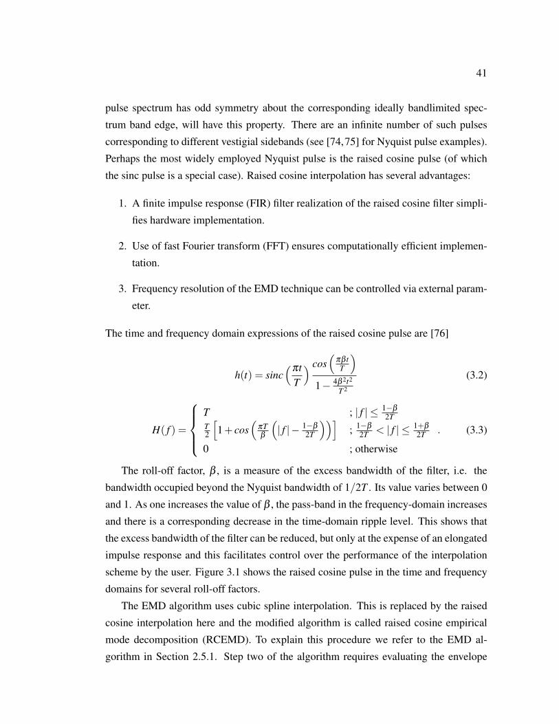
41
pulse spectrum has odd symmetry about the corresponding ideally bandlimited spec-
trum band edge, will have this property. There are an infinite number of such pulses
corresponding to different vestigial sidebands (see [74,75] for Nyquist pulse examples).
Perhaps the most widely employed Nyquist pulse is the raised cosine pulse (of which
the sinc pulse is a special case). Raised cosine interpolation has several advantages:
1. A finite impulse response (FIR) filter realization of the raised cosine filter simpli-
fies hardware implementation.
2. Use of fast Fourier transform (FFT) ensures computationally efficient implemen-
tation.
3. Frequency resolution of the EMD technique can be controlled via external param-
eter.
The time and frequency domain expressions of the raised cosine pulse are [76]
h(t) = sinc(πt
T
) cos(
πβ tT
)1− 4β 2t2
T 2
(3.2)
H( f ) =
T ; | f | ≤ 1−β
2TT2
[1+ cos
(πTβ
(| f |− 1−β
2T
))]; 1−β
2T < | f | ≤ 1+β2T
0 ; otherwise
. (3.3)
The roll-off factor, β , is a measure of the excess bandwidth of the filter, i.e. the
bandwidth occupied beyond the Nyquist bandwidth of 1/2T . Its value varies between 0
and 1. As one increases the value of β , the pass-band in the frequency-domain increases
and there is a corresponding decrease in the time-domain ripple level. This shows that
the excess bandwidth of the filter can be reduced, but only at the expense of an elongated
impulse response and this facilitates control over the performance of the interpolation
scheme by the user. Figure 3.1 shows the raised cosine pulse in the time and frequency
domains for several roll-off factors.
The EMD algorithm uses cubic spline interpolation. This is replaced by the raised
cosine interpolation here and the modified algorithm is called raised cosine empirical
mode decomposition (RCEMD). To explain this procedure we refer to the EMD al-
gorithm in Section 2.5.1. Step two of the algorithm requires evaluating the envelope
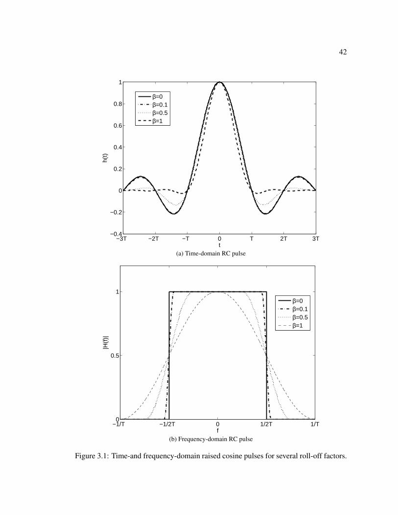
42
−3T −2T −T 0 T 2T 3T−0.4
−0.2
0
0.2
0.4
0.6
0.8
1
t
h(t)
β=0β=0.1β=0.5β=1
(a) Time-domain RC pulse
−1/T −1/2T 0 1/2T 1/T0
0.5
1
f
|H(f
)|
β=0β=0.1β=0.5β=1
(b) Frequency-domain RC pulse
Figure 3.1: Time-and frequency-domain raised cosine pulses for several roll-off factors.

43
values at intermediate points between successive extrema. In the original method the
cubic spline constructed of piecewise third-order polynomials is used. In the modified
method this is achieved by convolving the zero-padded sequence containing the extrema
with the raised cosine pulse. This can be implemented using an FIR filter in hardware.
The simplest member of this family, the sinc pulse (β = 0), has the added advantage
of ideal low-pass frequency characteristics, for an infinite length sequence. However, a
consequence of the ideal frequency behavior of the sinc pulse is that a filter implement-
ing the sinc pulse is extremely sensitive to non-uniformity in sampling, resulting in poor
performance relative to the cubic spline.
The sinc filter is highly sensitive to non-uniform sampling points due to slow decay
of the pulse. The rate of decay of the tails of the raised cosine pulse increases with the
roll-off factor and this makes it less sensitive to sampling point errors [76]. However,
increasing the roll-off factor also has the effect of increased filter bandwidth, thereby
reducing its frequency resolution. So, to summarize, increasing the roll-off factor 0
through 1 has two conflicting consequences: it decreases the sensitivity of the filter to
sampling point errors, but simultaneously reduces its frequency resolution. In section
3.4.1 we introduce a two-tone signal model to study the performance of the two inter-
polating techniques, where it has been previously shown [61] that the uniformity of the
spacing between the sampling points (local maxima or minima) is determined by the
ratio A2A1
f2f1≡ Γ, where A1, A2, f1 and f2 represent the amplitudes and frequencies of
the two tones. When Γ ≪ 1, the sampling points are nearly equidistant and the choice
of raised cosine pulse roll-off factor does not affect the frequency resolution of the al-
gorithm. However, a pulse with a smaller roll-off factor (β close to 0) can resolve the
signal components in fewer iterations and should therefore be preferred. When Γ ≪ 1 is
not satisfied, the spacings between consecutive local maxima and minima are no longer
approximately uniform causing a raised cosine interpolator with small β to fail in signal
separation and a larger roll-off factor is required.
FIR filter implementation is a major advantage of raised cosine interpolation. Filter
coefficients are determined by two parameters: the roll-off factor, β and the sampling
period, T . The roll-off factor, β , is a pre-defined system parameter affecting frequency
resolution of the algorithm. The sampling period, T , on the other hand, which is the
mean duration between consecutive maxima (or minima), is a signal-dependent param-
eter that is estimated on a block-by-block basis as described in Section 3.3. The interpo-

44
lated envelope is derived by convolving the zero-padded vector containing the maxima
(or minima) with the filter tap values. Moreover, frequency-domain implementation re-
duces the computational complexity by replacing convolution by multiplication. So to
reduce computational steps we perform convolution in the frequency domain by trans-
forming the zero-padded time-domain signals into the frequency domain using FFT,
filtering by the estimated interpolation filter coefficients and subsequent reconversion to
time-domain via inverse FFT.
3.3 Raised Cosine Empirical Mode Decomposition
Signal interpolation using the raised cosine pulse requires approximately uniform spac-
ing between control points or knots. A large β results in faster decay of the interpolant
tails, thereby reducing its sensitivity to non-uniform sampling intervals. However, non-
stationary signals result in larger variations in sampling intervals which reduces the
effectiveness of a raised cosine pulse with large β as an interpolant. To solve this prob-
lem, the original signal is split into small, overlapping segments and interpolation using
the raised cosine pulse is applied to each of them individually. By careful choice of
the interpolation window length relative to the maximum rate of change of the signal
instantaneous frequency, approximately uniform sampling intervals can be ensured.
We now enumerate the steps involved in the RCEMD algorithm. First, various pa-
rameters and variables are initialized.
A. Set the roll-off factor β , window shape w (a rectangular window is used in our
analysis) and window size K (corresponding to the number of successive extrema
to be included in the window). Further, N and M refer to the data length and the
number of maxima or minima in the signal respectively.
B. Initialize emax[n] and emin[n] to N-length zero-vectors.
Then the main loop of the algorithm is as follows:
1. Identify the extrema of x[n].
2. For i = 1 : M−K do the following

45
(a) Define index q= ui..ui+K , where u j represents the position of the jth maxima
of x[n].
(b) Compute window coefficients w[q], according to the shape chosen in Step A.
(c) Compute the windowed upper envelope xupper[q] = w[q]× x[ui : ui+K].
(d) Compute T =
K−1∑
k=1x[uk+1]−x[uk]
K−1 .
(e) Compute raised cosine filter coefficients h[q] using pre-defined β and com-
puted T .
(f) Compute emax[q] = emax[q]+ xupper[q]∗h[q].
(g) Compute emin[q] similarly, by first computing xlower[q] (Repeat steps c)-f)
for emin[q]).
3. Compute m[n] = emin[n]+emax[n]2 .
4. Extract the detail d[n] = x[n]−m[n].
5. If d[n] satisfies all IMF conditions, then set y1[n] = d[n], the first IMF, else repeat
above steps with d[n].
6. Evaluate the residual x1[n] = x[n]− y1[n].
7. Iterate on the residual x1[n].
The proposed algorithm differs from the original EMD algorithm in two crucial
ways: firstly, a new interpolant is used; and secondly, signal filtering is performed at
the local level. In our experiments we have found that window spanning five consecutive
extrema (either minima or maxima), i.e., K = 5 produces good signal resolution for a
wide variety of cases and has therefore been used consistently in all simulations. Signal
resolution performance and convergence rate comparison with EMD, which are consid-
ered in the following section, ignore boundary condition remediation operations such as
signal mirrorizing. In general, the effect of signal boundary on the RCEMD algorithm
was not found to be any worse than that for EMD, either in extent or severity, for the
examples considered here, but a detailed analysis of this phenomenon is relegated to
future research. Finally, β = 1 is used in all simulation results presented to minimize
the effect of non-uniform sampling.

46
3.4 Signal Decomposition Quality of RCEMD Algorithm
3.4.1 Combination of tones
Frequency resolution of RCEMD and EMD algorithms for a combination of two tones
is studied here. Mathematically, these signals are defined as
x(t) = s1(t)+ s2(t) (3.4)
where
s1(t) = A1sin(2π f1t +ϕ1)
s2(t) = A2sin(2π f2t +ϕ2) . (3.5)
and the symbols have their usual meanings and f1 > f2. Two metrics that measure the
similarity between the extracted IMFs and original tones are defined as
Ωk1 =
⟨s1(t)y1(t)⟩⟨s12(t)⟩
(3.6)
Ωk2 =
⟨s2(t)y2(t)⟩⟨s22(t)⟩
(3.7)
where y1(t) and y2(t) represent the extracted IMFs after k iterations of the algorithm and
⟨.⟩ denotes time-averaging. These quantities assume values between 0 and 1 with large
values indicating better signal decomposition quality. Signal separation performance of
the two algorithms for bicomponent signals considered in the present and following ex-
amples is based on Ωk2. This choice is based on the observation that due to the presence
of only two signal components and two extracted IMFs, a strong match between one sig-
nal component and a particular IMF implies strong match between the other signal and
the other IMF, thereby rendering Ωk1, Ωk
2 or a combined metric (such as their mean) as
equivalent measures of signal decomposition quality. Based on this decomposition qual-
ity metric we can state the following theorem for EMD performance using an arbitrary
interpolating filter:
Theorem 1. Suppose H( f ) denotes the frequency response of the interpolating filter.
Suppose further that A2A1
f2f1≪ 1 is satisfied. Then, Ωk
2 = 1− (1−H( f2))k.

47
Proof. Starting from (3.5) we observe that in the EMD technique the composite signal
is sampled at the local maxima and minima to obtain the upper and lower envelopes
respectively. These sampling points should ideally coincide with the extrema of the
high frequency (HF) component. We denote these ideal sampling instants by tu1 and t l
1
for the local maxima and minima respectively
tu1 = (4m−3) 1
4 f1− ϕ1
2π f1(3.8)
t l1 = (4m−1) 1
4 f1− ϕ1
2π f1(3.9)
for m= 1,2,3, ... with the sub-script indicating that these time instants refer to the higher
tone. Sampling the composite signal at these ideal sampling instants yields the lower
frequency tone offset by a constant value (A1 for the upper envelope and −A1 in case
of the lower envelope). However, estimation of the local extrema from the composite
signal by evaluating the derivative leads to errors resulting in actual sampling points (tu1 ,
t l1) that are different from the ideal sampling points (tu
1 , t l1). Figure 3.2 illustrates the
sampling point error described here.
Next we derive the expression for the upper envelope sampled at the points obtained
by determining the location of sign change of the derivative of x(t). The technique
described here can be adapted to derive the expression for the lower envelope also. We
have for the upper envelope
eu(tu1) = A1sin(2π f1tu
1 +ϕ1)+A2sin(2π f2tu1 +ϕ2) (3.10)
= A1sin(2π f1(tu
1 + tuδ )+ϕ1
)+A2sin(2π f2tu
1 +ϕ2) (3.11)
= A1sin(2π f1tu1 +ϕ1)cos(2π f1tu
δ )
+A1cos(2π f1tu1 +ϕ1)sin(2π f1tu
δ )
+A2sin(2π f2tu1 +ϕ2)
(3.12)
= A1cos(2π f1tuδ )+A2sin(2π f2tu
1 +ϕ2) (3.13)
≈ A1
(1−
4π2 f 21 tu
δ2
2
)+A2sin(2π f2tu
1 +ϕ2) (3.14)
≈ A1 −A12π2 f 21 tu
δ2 +A2sin(2π f2tu
1 +ϕ2). (3.15)
The term within the big parentheses in (3.14) follows from the Taylor series expansion
48
0 0.5 1 1.5 2 2.5 3 3.5 40
0.2
0.4
0.6
0.8
1
1.2
1.4
1.6
1.8
2
t (s)
s 1(t)
s1(t)
t1u
t1u+tδ
u
Figure 3.2: Positions of the HF component maxima and local maxima of the compositesignal superimposed on the HF component. The maximum separation between the twodepends on the relative amplitudes and frequencies of the signal components.
of the cosine term in (3.13), followed by its truncation after the first two terms. Of
course this approximation is valid only when 2π f1tuδ ≪ 1. The sampling error (tu
δ ) is
tuδ =
12π
A2
A1
f2
f 21
cos(2π f2tu1 +ϕm). (3.16)
The proof for this formula is given in Appendix . The values of tuδ computed from (3.16)
and those obtained from simulation are shown in Fig. 3.3. Further, we can write
tuδ
2 =1
4π2
(A2
A1
f2
f 21
)2
cos2(2π fmtu1 +ϕm). (3.17)
where fm = f12 −
∣∣∣ f12 −mod(2 f2, f1)
∣∣∣ is the possibly aliased version of 2 f2 and ϕm = ϕ2.
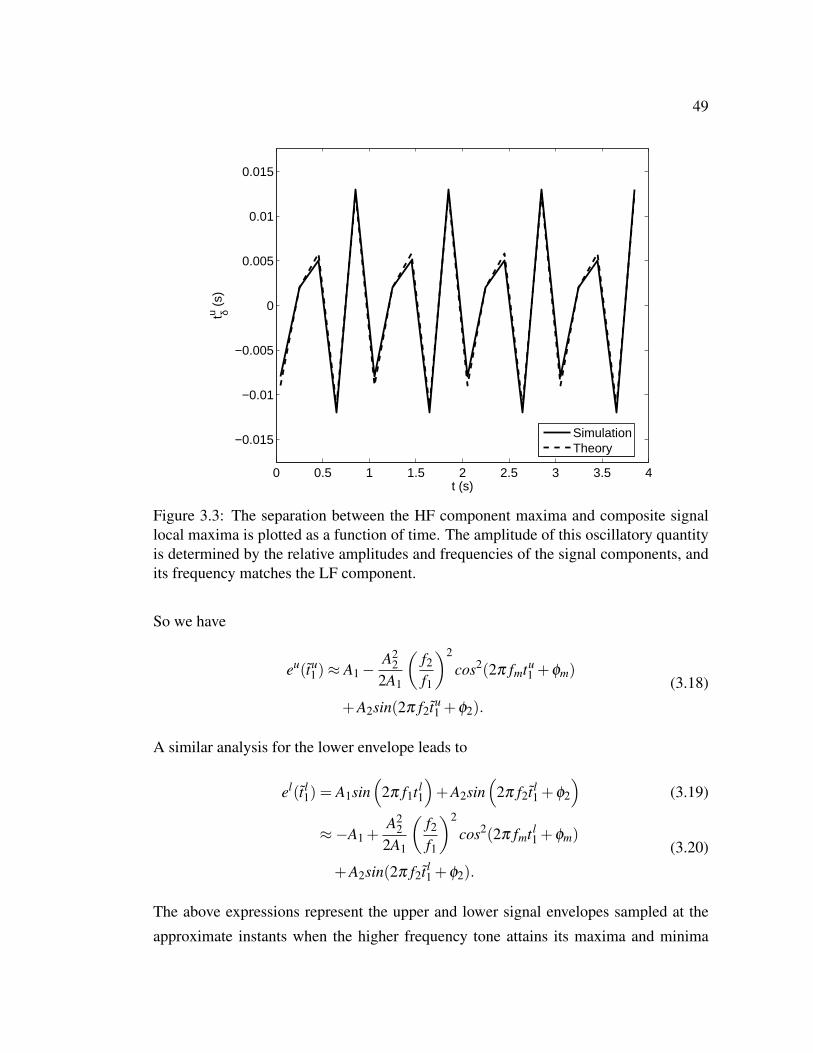
49
0 0.5 1 1.5 2 2.5 3 3.5 4
−0.015
−0.01
−0.005
0
0.005
0.01
0.015
t (s)
t δu (s)
SimulationTheory
Figure 3.3: The separation between the HF component maxima and composite signallocal maxima is plotted as a function of time. The amplitude of this oscillatory quantityis determined by the relative amplitudes and frequencies of the signal components, andits frequency matches the LF component.
So we have
eu(tu1)≈ A1 −
A22
2A1
(f2
f1
)2
cos2(2π fmtu1 +ϕm)
+A2sin(2π f2tu1 +ϕ2).
(3.18)
A similar analysis for the lower envelope leads to
el(t l1) = A1sin
(2π f1t l
1
)+A2sin
(2π f2t l
1 +ϕ2
)(3.19)
≈−A1 +A2
22A1
(f2
f1
)2
cos2(2π fmt l1 +ϕm)
+A2sin(2π f2t l1 +ϕ2).
(3.20)
The above expressions represent the upper and lower signal envelopes sampled at the
approximate instants when the higher frequency tone attains its maxima and minima

50
respectively. The preceding derivation assumes that 2π f1tuδ ≪ 1 and 2π f1t l
δ ≪ 1. These
conditions are satisfied when tuδ ≪ 1
2π f1and t l
δ ≪ 12π f1
respectively and from (3.16)
we can see that fulfillment of the first condition requires that A2A1
f2f1≪ 1 for the upper
envelope. A similar argument holds true for the lower signal envelope.
It is reasonable to assume that the sampling points of the envelopes are approxi-
mately equidistant as long as the condition A2A1
f2f1≪ 1 holds. In that case, interpolation of
the sparsely sampled envelopes leads to reconstruction of the continuous-time version
of the signal envelopes with the different frequency components weighted by the gain
derived from the frequency response of the interpolator, H( f )
eu(t)≈ H(0)A1 −H( fm)A2
2A1
(f2
2 f1
)2
sin2(2π fmt +ϕm)
+H( f2)A2sin(2π f2t +ϕ2)
(3.21)
el(t)≈−H(0)A1 +H( fm)A2
2A1
(f2
2 f1
)2
sin2(2π fmt +ϕm)
+H( f2)A2sin(2π f2t +ϕ2).
(3.22)
The mean (m1(t)) is simply the average of the two signal envelopes
m1(t) = H( f2)A2sin(2π f2t +ϕ2). (3.23)
The detail (d1(t)) is then given by d1(t) = x(t)−m1(t). So
d1(t) = A1sin(2π f1t +ϕ1)+(1−H( f2))A2sin(2π f2t +ϕ2) (3.24)
where the superscript 1 in d1(t) and m1(t) indicates that these quantities refer to the
detail and mean signals after the first EMD iteration. The next iteration of the EMD
algorithm continues with d1(t) as the new starting signal and the process continues
until some stopping criterion is fulfilled. Recalling that the original signal has only
two components we can conclude that the detail signal (dk(t)) and the residual (rk(t) =
x(t)−dk(t)) after k iterations should be sufficient to represent the individual components
and when dk(t) satisfies some stopping criterion, we stop iterating and dk(t) and rk(t)
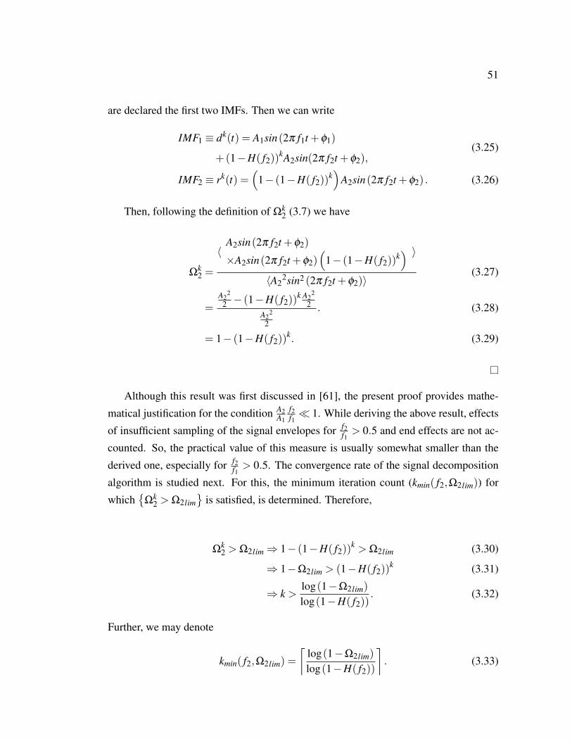
51
are declared the first two IMFs. Then we can write
IMF1 ≡ dk(t) = A1sin(2π f1t +ϕ1)
+(1−H( f2))kA2sin(2π f2t +ϕ2),
(3.25)
IMF2 ≡ rk(t) =(
1− (1−H( f2))k)
A2sin(2π f2t +ϕ2) . (3.26)
Then, following the definition of Ωk2 (3.7) we have
Ωk2 =
⟨A2sin(2π f2t +ϕ2)
×A2sin(2π f2t +ϕ2)(
1− (1−H( f2))k) ⟩
⟨A22sin2 (2π f2t +ϕ2)⟩
(3.27)
=A2
2
2 − (1−H( f2))k A2
2
2A2
2
2
. (3.28)
= 1− (1−H( f2))k. (3.29)
Although this result was first discussed in [61], the present proof provides mathe-
matical justification for the condition A2A1
f2f1≪ 1. While deriving the above result, effects
of insufficient sampling of the signal envelopes for f2f1> 0.5 and end effects are not ac-
counted. So, the practical value of this measure is usually somewhat smaller than the
derived one, especially for f2f1> 0.5. The convergence rate of the signal decomposition
algorithm is studied next. For this, the minimum iteration count (kmin( f2,Ω2lim)) for
which
Ωk2 > Ω2lim
is satisfied, is determined. Therefore,
Ωk2 > Ω2lim ⇒ 1− (1−H( f2))
k > Ω2lim (3.30)
⇒ 1−Ω2lim > (1−H( f2))k (3.31)
⇒ k >log(1−Ω2lim)
log(1−H( f2)). (3.32)
Further, we may denote
kmin( f2,Ω2lim) =
⌈log(1−Ω2lim)
log(1−H( f2))
⌉. (3.33)
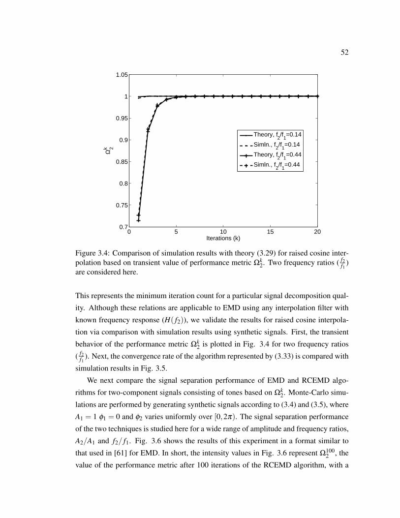
52
0 5 10 15 200.7
0.75
0.8
0.85
0.9
0.95
1
1.05
Iterations (k)
Ω2k
Theory, f2/f
1=0.14
Simln., f2/f
1=0.14
Theory, f2/f
1=0.44
Simln., f2/f
1=0.44
Figure 3.4: Comparison of simulation results with theory (3.29) for raised cosine inter-polation based on transient value of performance metric Ωk
2. Two frequency ratios ( f2f1
)are considered here.
This represents the minimum iteration count for a particular signal decomposition qual-
ity. Although these relations are applicable to EMD using any interpolation filter with
known frequency response (H( f2)), we validate the results for raised cosine interpola-
tion via comparison with simulation results using synthetic signals. First, the transient
behavior of the performance metric Ωk2 is plotted in Fig. 3.4 for two frequency ratios
( f2f1
). Next, the convergence rate of the algorithm represented by (3.33) is compared with
simulation results in Fig. 3.5.
We next compare the signal separation performance of EMD and RCEMD algo-
rithms for two-component signals consisting of tones based on Ωk2. Monte-Carlo simu-
lations are performed by generating synthetic signals according to (3.4) and (3.5), where
A1 = 1 ϕ1 = 0 and ϕ2 varies uniformly over [0,2π). The signal separation performance
of the two techniques is studied here for a wide range of amplitude and frequency ratios,
A2/A1 and f2/ f1. Fig. 3.6 shows the results of this experiment in a format similar to
that used in [61] for EMD. In short, the intensity values in Fig. 3.6 represent Ω1002 , the
value of the performance metric after 100 iterations of the RCEMD algorithm, with a
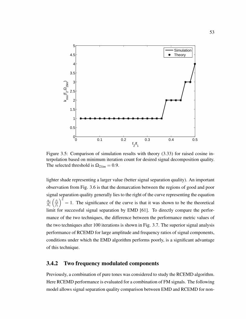
53
0 0.1 0.2 0.3 0.4 0.50
0.5
1
1.5
2
2.5
3
3.5
4
4.5
5
f2/f
1
k min
(f2,Ω
2lim
)
SimulationTheory
Figure 3.5: Comparison of simulation results with theory (3.33) for raised cosine in-terpolation based on minimum iteration count for desired signal decomposition quality.The selected threshold is Ω2lim = 0.9.
lighter shade representing a larger value (better signal separation quality). An important
observation from Fig. 3.6 is that the demarcation between the regions of good and poor
signal separation quality generally lies to the right of the curve representing the equationA2A1
(f2f1
)2= 1. The significance of the curve is that it was shown to be the theoretical
limit for successful signal separation by EMD [61]. To directly compare the perfor-
mance of the two techniques, the difference between the performance metric values of
the two techniques after 100 iterations is shown in Fig. 3.7. The superior signal analysis
performance of RCEMD for large amplitude and frequency ratios of signal components,
conditions under which the EMD algorithm performs poorly, is a significant advantage
of this technique.
3.4.2 Two frequency modulated components
Previously, a combination of pure tones was considered to study the RCEMD algorithm.
Here RCEMD performance is evaluated for a combination of FM signals. The following
model allows signal separation quality comparison between EMD and RCEMD for non-

54
A2
A1
(
f2
f1
)2
= 1 −→
log(A2/A
1)
f 2/f 1
−2 −1.5 −1 −0.5 0 0.5 1 1.5 2
0.1
0.2
0.3
0.4
0.5
0.6
0.7
0.8
0.9
0
0.1
0.2
0.3
0.4
0.5
0.6
0.7
0.8
0.9
1
Figure 3.6: Final value of the performance metric after 100 iterations(Ω1002 ) of the
RCEMD algorithm plotted for a range of amplitude and frequency ratios. A curve repre-senting the theoretical limit for successful signal separation by EMD [61] is also shown.
stationary components. This is similar to the non-stationary signal model used in [32,61]
EMD performance evaluation.
The FM signals can be represented as
sp(t) = Apcos(ωct + k f
t∫−∞
mp(τ)dτ +θp) (3.34)
and
mp(t) = Ampcos(ωpt +ϕp)+Bmp (3.35)
where p = 1,2. Then the instantaneous frequencies of the signals are given by
ωIp(t) = ωc + k f mp(t) , p = 1,2. (3.36)
In this signal model each signal component has four adjustable parameters affecting
the instantaneous frequency: Amp , Bmp , ωp and ϕp. The relation between Amp and Bmp

55
log(A2/A
1)
f 2/f 1
−2 −1.5 −1 −0.5 0 0.5 1 1.5 2
0.1
0.2
0.3
0.4
0.5
0.6
0.7
0.8
0.9
Figure 3.7: Differences between the final values of the performance metric after100 iterations of the two techniques,
[ω100
2]
RCEMD −[ω100
2]
EMD. The differencesare quantized to three values: 1, signifying that performance of RCEMD is better([
ω1002]
RCEMD −[ω100
2]
EMD ≥ 0.05); -1, signifying that performance of EMD is better([
ω1002]
EMD −[ω100
2]
RCEMD ≥ 0.05); 0, signifying that the performance of both tech-
niques is about the same(∣∣[ω100
2]
RCEMD −[ω100
2]
EMD
∣∣< 0.05). The regions represent-
ing the values 1 and 0 are in white and black respectively. The value -1 does not appearin this graph.
and their effect on the instantaneous frequency are shown in Fig. 3.8. Moreover, ωp
and ϕp control the starting phase and the rate of change of the instantaneous frequen-
cies of the two signals, respectively. So, while ωp determines the starting phase of the
instantaneous frequencies in Fig. 3.8, their oscillation frequencies depend on ωp. From
the figure it is clear that the parameters Amp and Bmp determine the relative frequency
separation between the components and, consequently, the level of difficulty for signal
separation. In our experiments we fix the parameters of signal s2(t) and vary those of
s1(t) to achieve different frequency compositions of the component signals. Moreover,
ωp and ϕp are identical for the two components to prevent crossing of instantaneous
frequencies.
Signal separation quality of the two algorithms is evaluated based on the metric Ω1002
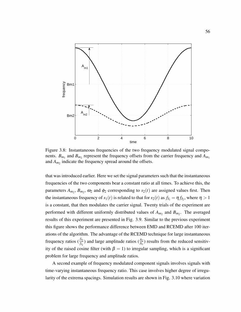
56
0 2 4 6 8 10
Bm2
Bm1
time
freq
uenc
y
Am2
Am1
Figure 3.8: Instantaneous frequencies of the two frequency modulated signal compo-nents. Bm1 and Bm2 represent the frequency offsets from the carrier frequency and Am1
and Am2 indicate the frequency spread around the offsets.
that was introduced earlier. Here we set the signal parameters such that the instantaneous
frequencies of the two components bear a constant ratio at all times. To achieve this, the
parameters Am2 , Bm2 , ω2 and ϕ2 corresponding to s2(t) are assigned values first. Then
the instantaneous frequency of s1(t) is related to that for s2(t) as fI1 = η fI2 , where η > 1
is a constant, that then modulates the carrier signal. Twenty trials of the experiment are
performed with different uniformly distributed values of Am2 and Bm2 . The averaged
results of this experiment are presented in Fig. 3.9. Similar to the previous experiment
this figure shows the performance difference between EMD and RCEMD after 100 iter-
ations of the algorithm. The advantage of the RCEMD technique for large instantaneous
frequency ratios (fI2fI1
) and large amplitude ratios (A2A1
) results from the reduced sensitiv-
ity of the raised cosine filter (with β = 1) to irregular sampling, which is a significant
problem for large frequency and amplitude ratios.
A second example of frequency modulated component signals involves signals with
time-varying instantaneous frequency ratio. This case involves higher degree of irregu-
larity of the extrema spacings. Simulation results are shown in Fig. 3.10 where variation
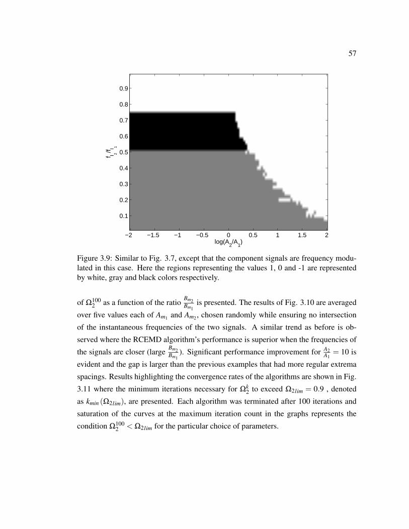
57
log(A2/A
1)
f I 2/f I 1
−2 −1.5 −1 −0.5 0 0.5 1 1.5 2
0.1
0.2
0.3
0.4
0.5
0.6
0.7
0.8
0.9
Figure 3.9: Similar to Fig. 3.7, except that the component signals are frequency modu-lated in this case. Here the regions representing the values 1, 0 and -1 are representedby white, gray and black colors respectively.
of Ω1002 as a function of the ratio
Bm2Bm1
is presented. The results of Fig. 3.10 are averaged
over five values each of Am1 and Am2 , chosen randomly while ensuring no intersection
of the instantaneous frequencies of the two signals. A similar trend as before is ob-
served where the RCEMD algorithm’s performance is superior when the frequencies of
the signals are closer (largeBm2Bm1
). Significant performance improvement for A2A1
= 10 is
evident and the gap is larger than the previous examples that had more regular extrema
spacings. Results highlighting the convergence rates of the algorithms are shown in Fig.
3.11 where the minimum iterations necessary for Ωk2 to exceed Ω2lim = 0.9 , denoted
as kmin (Ω2lim), are presented. Each algorithm was terminated after 100 iterations and
saturation of the curves at the maximum iteration count in the graphs represents the
condition Ω1002 < Ω2lim for the particular choice of parameters.

58
0 0.2 0.4 0.6 0.8 10.2
0.3
0.4
0.5
0.6
0.7
0.8
0.9
1
Bm
2
/Bm
1
Ω210
0 Raised CosineCubic Spline
(a) A2A1
= 1
0 0.2 0.4 0.6 0.8 10.2
0.3
0.4
0.5
0.6
0.7
0.8
0.9
1
Bm
2
/Bm
1
Ω210
0 Raised CosineCubic Spline
(b) A2A1
= 0.1
Figure 3.10
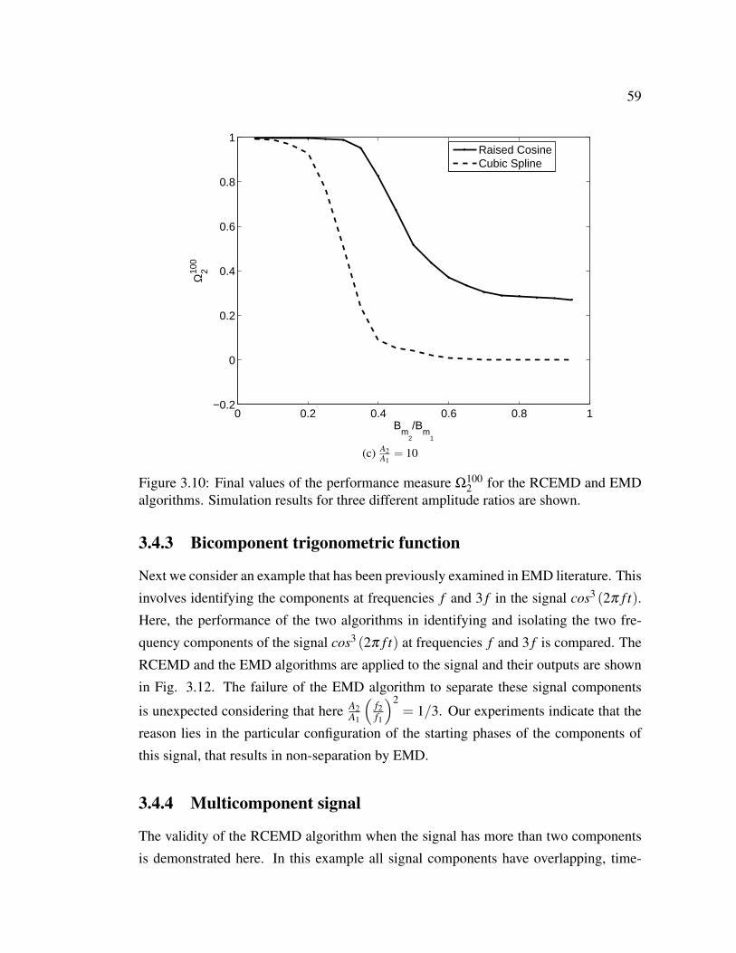
59
0 0.2 0.4 0.6 0.8 1−0.2
0
0.2
0.4
0.6
0.8
1
Bm
2
/Bm
1
Ω210
0
Raised CosineCubic Spline
(c) A2A1
= 10
Figure 3.10: Final values of the performance measure Ω1002 for the RCEMD and EMD
algorithms. Simulation results for three different amplitude ratios are shown.
3.4.3 Bicomponent trigonometric function
Next we consider an example that has been previously examined in EMD literature. This
involves identifying the components at frequencies f and 3 f in the signal cos3 (2π f t).
Here, the performance of the two algorithms in identifying and isolating the two fre-
quency components of the signal cos3 (2π f t) at frequencies f and 3 f is compared. The
RCEMD and the EMD algorithms are applied to the signal and their outputs are shown
in Fig. 3.12. The failure of the EMD algorithm to separate these signal components
is unexpected considering that here A2A1
(f2f1
)2= 1/3. Our experiments indicate that the
reason lies in the particular configuration of the starting phases of the components of
this signal, that results in non-separation by EMD.
3.4.4 Multicomponent signal
The validity of the RCEMD algorithm when the signal has more than two components
is demonstrated here. In this example all signal components have overlapping, time-

60
0 0.2 0.4 0.6 0.8 110
0
101
102
Bm
2
/Bm
1
k min
(Ω2l
im)
Raised CosineCubic Spline
(a) A2A1
= 1
0 0.2 0.4 0.6 0.8 110
0
101
102
Bm
2
/Bm
1
k min
(Ω2l
im)
Raised CosineCubic Spline
(b) A2A1
= 0.1
Figure 3.11

61
0 0.2 0.4 0.6 0.8 110
0
101
102
Bm
2
/Bm
1
k min
(Ω2l
im)
Raised CosineCubic Spline
(c) A2A1
= 10
Figure 3.11: Minimum number of iterations necessary for Ωk2 to exceed Ω2lim = 0.9
for the windowed RCEMD and EMD algorithms. Simulation results for three differentamplitude ratios are shown.
varying instantaneous frequencies that are difficult to separate using traditional filtering
techniques. Moreover, two of the signal components have time-varying amplitudes also,
meaning that the amplitudes Ap in (3.34) are now time-varying for two of the three sig-
nal components (here p = 1,2,3). Successful signal decomposition using EMD for a
similar signal has been previously demonstrated [61]. Here we test the ability of the
RCEMD algorithm to decompose the signals. The frequency-and time-domain signals
are shown in Fig. 3.13 and Fig. 3.14 respectively. Although, the signals have been cor-
rectly separated into their respective IMFs, some signal-mixing is evident in regions of
small instantaneous frequencies for this difficult signal separation problem. This is be-
cause there are fewer cycles of the signal over these intervals that results in an elongated
RCEMD window, the length of which depends on inter-extrema spacing. The windowed
signal no longer has constant instantaneous frequency over the extended interval, result-
ing in non-optimum filtering. This effect, which is seen when the signal components
have small instantaneous frequencies, is not observed for EMD.
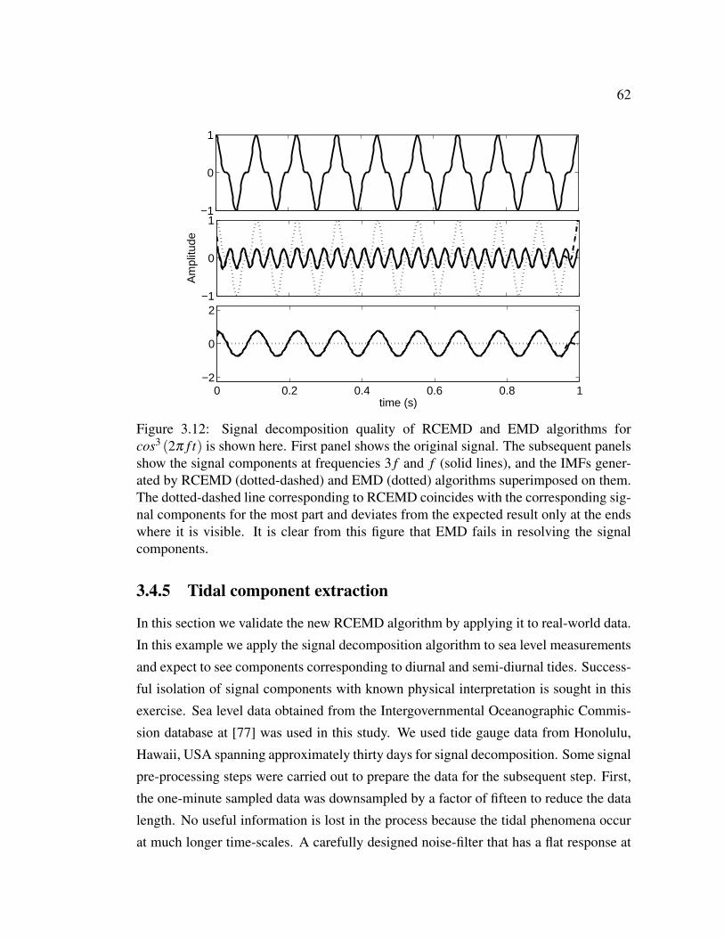
62
−1
0
1
−1
0
1
Am
plitu
de
0 0.2 0.4 0.6 0.8 1−2
0
2
time (s)
Figure 3.12: Signal decomposition quality of RCEMD and EMD algorithms forcos3 (2π f t) is shown here. First panel shows the original signal. The subsequent panelsshow the signal components at frequencies 3 f and f (solid lines), and the IMFs gener-ated by RCEMD (dotted-dashed) and EMD (dotted) algorithms superimposed on them.The dotted-dashed line corresponding to RCEMD coincides with the corresponding sig-nal components for the most part and deviates from the expected result only at the endswhere it is visible. It is clear from this figure that EMD fails in resolving the signalcomponents.
3.4.5 Tidal component extraction
In this section we validate the new RCEMD algorithm by applying it to real-world data.
In this example we apply the signal decomposition algorithm to sea level measurements
and expect to see components corresponding to diurnal and semi-diurnal tides. Success-
ful isolation of signal components with known physical interpretation is sought in this
exercise. Sea level data obtained from the Intergovernmental Oceanographic Commis-
sion database at [77] was used in this study. We used tide gauge data from Honolulu,
Hawaii, USA spanning approximately thirty days for signal decomposition. Some signal
pre-processing steps were carried out to prepare the data for the subsequent step. First,
the one-minute sampled data was downsampled by a factor of fifteen to reduce the data
length. No useful information is lost in the process because the tidal phenomena occur
at much longer time-scales. A carefully designed noise-filter that has a flat response at
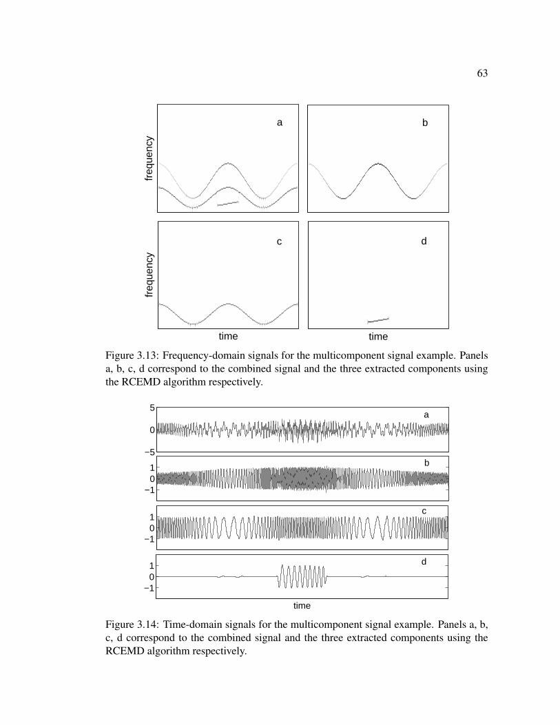
63
freq
uenc
y
time
freq
uenc
y
time
a b
c d
Figure 3.13: Frequency-domain signals for the multicomponent signal example. Panelsa, b, c, d correspond to the combined signal and the three extracted components usingthe RCEMD algorithm respectively.
−5
0
5
−101
−101
−101
time
a
b
c
d
Figure 3.14: Time-domain signals for the multicomponent signal example. Panels a, b,c, d correspond to the combined signal and the three extracted components using theRCEMD algorithm respectively.
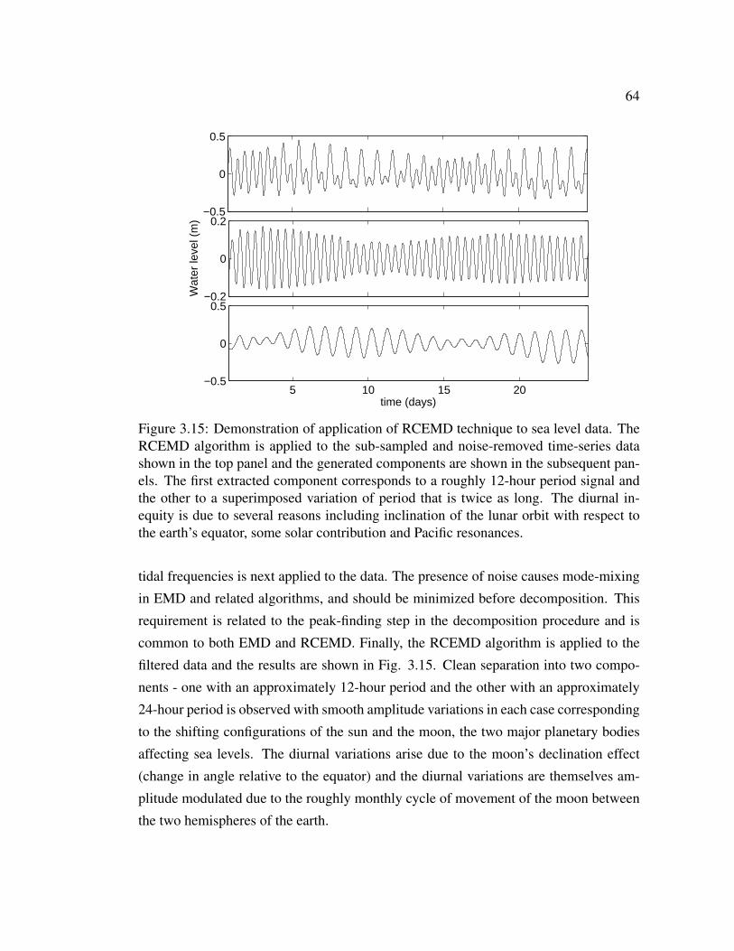
64
−0.5
0
0.5
−0.2
0
0.2
Wat
er le
vel (
m)
5 10 15 20−0.5
0
0.5
time (days)
Figure 3.15: Demonstration of application of RCEMD technique to sea level data. TheRCEMD algorithm is applied to the sub-sampled and noise-removed time-series datashown in the top panel and the generated components are shown in the subsequent pan-els. The first extracted component corresponds to a roughly 12-hour period signal andthe other to a superimposed variation of period that is twice as long. The diurnal in-equity is due to several reasons including inclination of the lunar orbit with respect tothe earth’s equator, some solar contribution and Pacific resonances.
tidal frequencies is next applied to the data. The presence of noise causes mode-mixing
in EMD and related algorithms, and should be minimized before decomposition. This
requirement is related to the peak-finding step in the decomposition procedure and is
common to both EMD and RCEMD. Finally, the RCEMD algorithm is applied to the
filtered data and the results are shown in Fig. 3.15. Clean separation into two compo-
nents - one with an approximately 12-hour period and the other with an approximately
24-hour period is observed with smooth amplitude variations in each case corresponding
to the shifting configurations of the sun and the moon, the two major planetary bodies
affecting sea levels. The diurnal variations arise due to the moon’s declination effect
(change in angle relative to the equator) and the diurnal variations are themselves am-
plitude modulated due to the roughly monthly cycle of movement of the moon between
the two hemispheres of the earth.
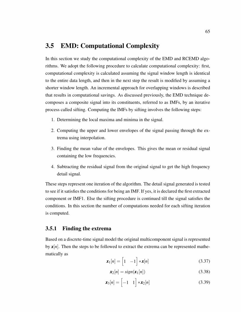
65
3.5 EMD: Computational Complexity
In this section we study the computational complexity of the EMD and RCEMD algo-
rithms. We adopt the following procedure to calculate computational complexity: first,
computational complexity is calculated assuming the signal window length is identical
to the entire data length, and then in the next step the result is modified by assuming a
shorter window length. An incremental approach for overlapping windows is described
that results in computational savings. As discussed previously, the EMD technique de-
composes a composite signal into its constituents, referred to as IMFs, by an iterative
process called sifting. Computing the IMFs by sifting involves the following steps:
1. Determining the local maxima and minima in the signal.
2. Computing the upper and lower envelopes of the signal passing through the ex-
trema using interpolation.
3. Finding the mean value of the envelopes. This gives the mean or residual signal
containing the low frequencies.
4. Subtracting the residual signal from the original signal to get the high frequency
detail signal.
These steps represent one iteration of the algorithm. The detail signal generated is tested
to see if it satisfies the conditions for being an IMF. If yes, it is declared the first extracted
component or IMF1. Else the sifting procedure is continued till the signal satisfies the
conditions. In this section the number of computations needed for each sifting iteration
is computed.
3.5.1 Finding the extrema
Based on a discrete-time signal model the original multicomponent signal is represented
by xxx[n]. Then the steps to be followed to extract the extrema can be represented mathe-
matically as
xxx1[n] =[1 −1
]∗xxx[n] (3.37)
xxx2[n] = sign(xxx1[n]) (3.38)
xxx3[n] =[−1 1
]∗xxx2[n] (3.39)

66
Table 3.1: No. of computations to find extrema points
Equation Operation count3.37 N3.38 N3.39 N3.40a 2N3.40b 2N3.41a N3.41b NTotal 9N
xxx41 [n] =|sign(xxx3[n])|+xxx3[n]/2
2(3.40a)
xxx42[n] =−|sign(xxx3[n])|+xxx3[n]/2
2(3.40b)
xxx51[n] = xxx41[n]⊗xxx[n] (3.41a)
xxx52 [n] =−xxx42[n]⊗xxx[n] (3.41b)
where ∗ denotes convolution and ⊗ denotes vector element-by-element multiplication.
Here in the first two steps we find the sign of the numerical derivative of the signal. In
step three we find the derivative of the result, which gives us the location of the signal
local maxima (where first derivative changes sign). Steps 4 and 5 find the locations
of the signal local maxima and minima respectively. In the last two steps the function
values at the local signal maxima and minima locations are evaluated. If there are N
samples in the data-set then the number of computations required for each mathematical
step above are listed in Table 3.1. The number of maxima (or minima) depends on the
number of complete cycles of the highest frequency component present in the signal, M.
3.5.2 Finding the cubic spline coefficients
A cubic spline is a spline constructed of piecewise third-order polynomials which pass
through a set of M control points. The second derivative of each polynomial is com-
monly set to zero at the endpoints, since this provides a boundary condition that com-
pletes the system of M − 1 equations. This produces a so-called “natural” cubic spline

67
and leads to a simple tridiagonal system which can be solved easily to give the coeffi-
cients of the polynomials. However, this choice is not the only one possible, and other
boundary conditions can be used instead.
We use the natural cubic spline system in our system as it leads to a tridiagonal
system of equations that can be solved in O(M −1) operations instead of O((M −1)3)
required by Gaussian elimination [78]. Specifically, in our case, 18M − 28 operations
are required for computing the piecewise cubic spline coefficients for either of the two
envelopes. Further, 21N operations are needed to find the residual and detail signals.
So in all (9N)+ 2(18M − 28)+ (21N) = 30N + 36M − 56 computations are required
for each sifting iteration of the EMD algorithm. Denoting by Si the number of sifting
iterations needed to generate IMFi, the total number of operations needed to extract
IMFi is simply obtained by multiplying the above expression by Si.
3.5.3 Complexity of the raised cosine filter approach
In addition to some extremely efficient hardware implementations of the FFT avail-
able ( [79, 80]), the fastest software implementation of the FFT algorithm requires
2N log2 N−3N+4 operations for real values [81]. A simple calculation of the operation
count for the raised cosine interpolation follows from this result. This approach involves
four steps: finding the mean of xxx51[n] and xxx52[n], computing the Fourier transform, mul-
tiplying by the frequency response of the filter and computing the inverse Fourier trans-
form. So, in all 2N+2N log2 N−3N+4+N+2N log2 N−3N+4= 4N log2 N−3N+8
operations are needed to compute the mean signal using the raised cosine filter approach
after evaluating xxx51[n] and xxx52[n] compared to 21N + 2(18M − 28) = 21N + 36M − 56
operations for the cubic spline technique for the corresponding steps. Finally, the over-
all operation count for separating two signals is obtained by multiplying the just-derived
operation counts per iteration by Si, the number of iterations needed by each algorithm
to achieve a certain signal separation quality. Moreover, it is seen that the operation
counts derived above can be split nearly in half between the number of multiplication
and divisions on one side and addition and subtraction on the other for both algorithms,
with the number of additions and subtractions slightly larger than the other group. Fi-
nally, we observe that per iteration, the RCEMD algorithm is generally faster than EMD
for shorter signal lengths.

68
0.1 0.2 0.3 0.4 0.5 0.6 0.7 0.8 0.9
105
106
Bm
2
/Bm
1
Ope
ratio
n co
unt
RC, A2/A
1=1
CS, A2/A
1=1
RC, A2/A
1=10
CS, A2/A
1=10
Figure 3.16: Computational complexity comparison for frequency modulated signalcomponents. Results for two amplitude ratios A2
A1= 1 and A2
A1= 10 are presented. Com-
putational complexity when A2A1
= 0.1 is similar to that for the equal amplitude case andis therefore omitted for clarity.
3.5.4 Complexity of windowed RCEMD
Next, we compare the computational complexity of the RCEMD and the EMD algo-
rithms applied to multicomponent signals with time-varying frequencies. In this case
a segment of the multicomponent signal containing K consecutive extrema (maxima or
minima) is decomposed at a time. So a window contains K NM ≡ L signal samples on an
average. After operating on a particular segment of the signal the window is advanced
to the next maxima or minima, while discarding the oldest data samples and the process
repeats until the entire signal is decomposed. By realizing that the operation count for
the first window being 4L log2 L−3L+8, and that IMF segments for the following seg-
ments can be computed by incrementally performing 2K times the number of operations
for the first window (corresponding to the first and the last inter-extrema samples for
each window), and that M−K shifts of the window are required, the resulting total op-
eration count per iteration is (2MK −1)(4L log2 L−3L+8). The total operation count to
decompose a multicomponent signal into two IMFs is arrived at by multiplying the per

69
iteration operation count by the number of iterations required to achieve desired signal
analysis quality. The operation counts of the RCEMD and EMD algorithms are shown
in Fig. 3.16. The plots saturate for largeBm2Bm1
due to the termination of the decomposi-
tion after 100 iterations. Rectangular window with K = 5 was used in the simulations.
To summarize, assuming uniform distribution of the ratioBm2Bm1
over the non-saturated
region of Fig. 3.16, on an average, the computational complexity of the EMD algorithm
is nearly twice and four times that of the RCEMD algorithm for comparable signal sep-
aration quality when A2A1
= 1 and A2A1
= 10 respectively.
3.6 Low Sampling Rate Performance of RCEMD
Successful signal analysis using the empirical mode decomposition (EMD) algorithm
requires high degree of oversampling. This requirement arises from the need to precisely
identify the local extrema of the signal to recover the signal envelope using natural
cubic spline interpolation. This problem is alleviated in RCEMD which allows high
fidelity reconstruction of the signal envelope when the local extrema cannot be precisely
identified due to low sampling rates. The advantage of this technique at low sampling
rates is demonstrated using synthetic signals in this section.
Reference [82] introduced a solution to the fast sampling requirement of the EMD
algorithm by using a new extrema identification procedure based on Fourier interpo-
lation. References [62] and [63] present further research on the effect of sampling on
EMD. Here, we demonstrate the advantage of the raised cosine interpolation-based tech-
nique introduced in this chapter at low sampling rates. The timing jitter problem at
low sampling rates is first introduced followed by some synthetic signal examples to
demonstrate the the superior signal analysis performance of RCEMD algorithm at low
sampling rates.
3.6.1 Timing jitter at low sampling rates
The effect of timing jitter on signal analysis performance using EMD is examined here.
For this, following a similar approach as our previous analysis in Section 3.4.1, we

70
consider an N-sample long two-tone signal,
s(tp) = A1sin(2π f1tp +ϕ1)+A2sin(2π f2tp +ϕ2) , (3.42)
where p = 1, ...,N, f1 > f2 and the symbols have the usual meanings. In the EMD algo-
rithm an estimate of the low frequency component is obtained by evaluating the average
of the upper and lower signal envelopes of the sampled multicomponent signal by inter-
polating between successive local maxima and minima respectively. If we denote by tm,
m = 1,2, ... the locations of the sampled composite signal local maxima, then the f1-rate
sampled upper envelope is given by
eu (tum) = A1sin(2π f1tu
m +ϕ1)+A2sin(2π f2tum +ϕ2) . (3.43)
If the envelopes are sampled at the exact peaks and troughs of the larger frequency
component, denoted by tum and t l
m respectively, then
eu (tum) = A1sin((m−1)2π +π/2)+A2sin(2π f2tu
m +ϕ2)
= A1 +A2sin(2π f2tum +ϕ2) . (3.44)
Similarly, el (t lm)=−A1+A2sin
(2π f2t l
m +ϕ2), so that the average of the two envelopes
interpolated to fs-rate closely approximates the smaller tone.
However, finite sampling rate introduces timing jitter that causes the actual sampling
points to deviate from the ideal ones. Denoting the timing error sequence by δ um, we find
that δ um = tu
m− tum, where δ u
m is uniformly distributed over (−1/2 fs,1/2 fs). The sampled
upper envelope can then be represented as
eu (tum) = A1sin((m−1)2π +π/2+2π f1δ u
m)+A2sin(2π f2 (t +mu +δ um)+ϕ2) .
(3.45)
Therefore, we find that finite sampling not only causes irregular sampling of the enve-
lope but also introduces a high frequency component at frequency f1. Raised cosine
interpolation using large β results in more accurate signal representation than natural
cubic splines when irregular sampling results in introduction of spurious high frequency
components as demonstrated by the following experiment.
We first choose the frequencies f1, f2 and sampling rate fs such that f2 < f1 ≤ fs/2.
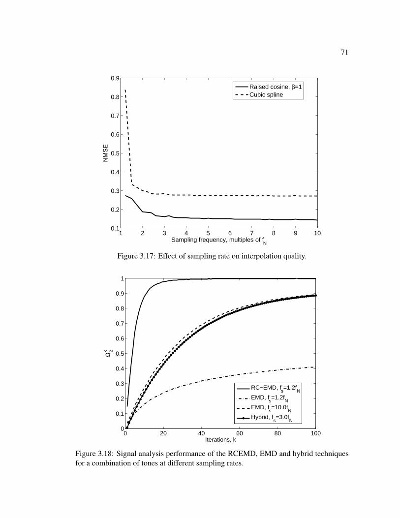
71
1 2 3 4 5 6 7 8 9 100.1
0.2
0.3
0.4
0.5
0.6
0.7
0.8
0.9
Sampling frequency, multiples of fN
NM
SE
Raised cosine, β=1Cubic spline
Figure 3.17: Effect of sampling rate on interpolation quality.
0 20 40 60 80 1000
0.1
0.2
0.3
0.4
0.5
0.6
0.7
0.8
0.9
1
Iterations, k
Ω2k
RC−EMD, fs=1.2f
N
EMD, fs=1.2f
N
EMD, fs=10.0f
N
Hybrid, fs=3.0f
N
Figure 3.18: Signal analysis performance of the RCEMD, EMD and hybrid techniquesfor a combination of tones at different sampling rates.

72
0 20 40 60 80 1000
0.1
0.2
0.3
0.4
0.5
0.6
0.7
0.8
0.9
1
Iterations, k
Ω2k
RC−EMD, fs=3f
N
EMD, fs=3f
N
EMD, fs=25f
N
Hybrid, fs=15f
N
Figure 3.19: Signal analysis performance of the RCEMD, EMD and hybrid techniquesfor a combination of frequency modulated signals at different sampling rates.
Our aim here is to recover the signal s2(t) = A2sin(2π f2t +ϕ2) at sampling rate fs from
the available irregularly-spaced samples at an average rate of f1. This sampled signal
also includes a higher frequency component at f1 as described above. We compare the
performances of two interpolation techniques: one using the raised cosine pulse with
β = 1, and the other using the natural cubic spline. Normalized mean squared error
(NMSE) is used as the performance criterion. The results are presented in Fig. 3.17 for
a range of sampling rates. Here A1 = A2 = 1, f2 = 0.5 f1 and the results are averaged
over several uniformly distributed starting phases and timing jitter realizations. It is clear
from the results that not only is the interpolation quality using raised cosine pulse better
than that using cubic splines, but the difference between them is larger at low sampling
rates, close to the Nyquist rate ( fN = 2 f1). This justifies the use of RCEMD procedure
that uses the raised cosine pulse for interpolation. In the next section we will compare
the signal analysis performance of this technique to EMD at low sampling rates.
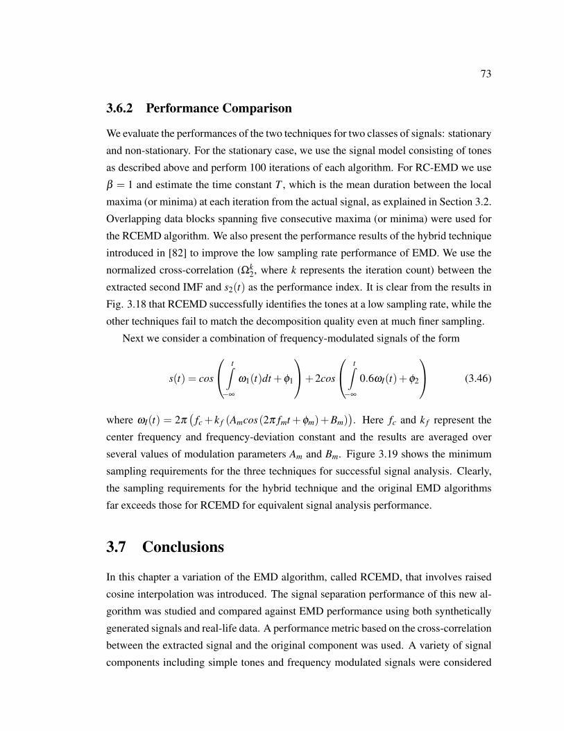
73
3.6.2 Performance Comparison
We evaluate the performances of the two techniques for two classes of signals: stationary
and non-stationary. For the stationary case, we use the signal model consisting of tones
as described above and perform 100 iterations of each algorithm. For RC-EMD we use
β = 1 and estimate the time constant T , which is the mean duration between the local
maxima (or minima) at each iteration from the actual signal, as explained in Section 3.2.
Overlapping data blocks spanning five consecutive maxima (or minima) were used for
the RCEMD algorithm. We also present the performance results of the hybrid technique
introduced in [82] to improve the low sampling rate performance of EMD. We use the
normalized cross-correlation (Ωk2, where k represents the iteration count) between the
extracted second IMF and s2(t) as the performance index. It is clear from the results in
Fig. 3.18 that RCEMD successfully identifies the tones at a low sampling rate, while the
other techniques fail to match the decomposition quality even at much finer sampling.
Next we consider a combination of frequency-modulated signals of the form
s(t) = cos
t∫−∞
ω1(t)dt +ϕ1
+2cos
t∫−∞
0.6ωI(t)+ϕ2
(3.46)
where ωI(t) = 2π(
fc + k f (Amcos(2π fmt +ϕm)+Bm)). Here fc and k f represent the
center frequency and frequency-deviation constant and the results are averaged over
several values of modulation parameters Am and Bm. Figure 3.19 shows the minimum
sampling requirements for the three techniques for successful signal analysis. Clearly,
the sampling requirements for the hybrid technique and the original EMD algorithms
far exceeds those for RCEMD for equivalent signal analysis performance.
3.7 Conclusions
In this chapter a variation of the EMD algorithm, called RCEMD, that involves raised
cosine interpolation was introduced. The signal separation performance of this new al-
gorithm was studied and compared against EMD performance using both synthetically
generated signals and real-life data. A performance metric based on the cross-correlation
between the extracted signal and the original component was used. A variety of signal
components including simple tones and frequency modulated signals were considered

74
for performance comparison. Relative superiority of the RCEMD technique for situ-
ations where signal separation is particularly difficult, such as when the instantaneous
frequencies of the components are similar or when the high frequency signal is weaker,
is a significant advantage of this technique. Further, successful signal decomposition
using the developed technique for a cubic sinusoid as well as a multicomponent sig-
nal case with both amplitude- and frequency-modulated components was demonstrated.
Reduced signal separation quality for very small signal instantaneous frequencies was
observed as a potential drawback of this technique. Validity of this technique was fur-
ther demonstrated by successful decomposition of real-world data into physically jus-
tifiable signal components. Thereafter, the two algorithms were compared based on
computational complexity. To achieve equivalent signal separation quality, the proposed
technique was shown to require fewer computations for particularly difficult signal de-
composition problems. Finally, it was shown that the RCEMD algorithm requires much
lower sampling rates than the EMD and an improved algorithm reported in literature to
resolve two signal components. Performance comparison of RCEMD algorithm with
other time-frequency analysis techniques, such as STFT and wavelets, follows in Chap-
ter 7 for microbarograph data.
Chapter 4
Pre-emphasis and De-emphasis
In this chapter we propose a new pre-emphasis and de-emphasis technique to improve
the frequency resolution of EMD for a particular configuration of tonal signals with
unequal amplitudes. Specifically, we present here a technique for improving the fre-
quency resolution of the EMD technique when the lower tone has a larger amplitude
by augmenting the higher tone before applying EMD and subsequently reversing the
effect of frequency augmentation after the decomposition is completed. Practical filters
to achieve pre-emphasis and de-emphasis are also introduced. Although this technique
was developed to improve the performance of the original EMD algorithm, it can be
applied to RCEMD also.
4.1 Introduction
In this chapter we present results of our study on the frequency resolution of EMD.
We demonstrate the effect of the choice of certain simulation control parameters on the
performance of the algorithm and also suggest a new pre-processing step that improves
its frequency resolution for simple tonal signals with unequal amplitudes.
In Section 4.3 we focus on the inability of EMD to extract closely spaced tones when
the lower tone is stronger. Although this problem is common to most time-frequency
analysis techniques, the performance of EMD is especially bad in this case. This is due
to the sequential nature of the technique where progressively lower frequency compo-
nent signals are extracted consecutively. So, failure in separating the tones in the first
step results in a single IMF to be generated by the procedure. To overcome this problem

76
we propose a technique where the original composite signal is pre-processed so that the
strength of the higher tone is artificially increased in relation to the lower tone before
performing EMD and the output from EMD is then compensated by a post-processing
step that seeks to undo the distortion caused by the pre-processor. The effectiveness of
this technique is demonstrated by simulations using synthetic signals.
Many researchers have attempted to provide an analytical framework for this empir-
ical technique [33, 47] and to gain better understanding about its working [59]. Some
of these works include the study of the effect of sampling on EMD [62, 63] and its in-
terpretation as a filter-bank [60]. Attempts to achieve better decomposition have led
researchers to suggest using masking signals [37] and white noise at the signal bound-
aries [67]. But relatively few works (e.g., [29,37,67] in parts) have considered the issue
of frequency resolution of the EMD algorithm which we aim to address in this chap-
ter. In this work we have utilized the package available at [83] to implement the EMD
technique.
4.2 Optimum choice of stopping criterion for sifting
The sifting iterations are terminated when the residual signal satisfies the conditions for
being an IMF. Two conditions are to be fulfilled in this respect [27]: the first one is
that the number of extrema and the number of zero-crossings must differ at most by 1;
and the second one is that the mean value of the upper and lower envelopes must be
close to zero by some criterion. The authors of [29] have come up with a parameter
that quantifies the second condition and lets the user set a pair of thresholds depending
on the required level of adherence to the second condition above. Although there is no
linear relation, generally large values for the thresholds result in fewer sifting iterations
whereas lower threshold values cause more sifting iterations to occur. In this section
we aim to demonstrate the effect of this stopping criterion as well as the choice of
maximum iteration limit on the performance of the EMD technique. For this purpose
we use a synthetically generated signal consisting of two closely spaced tones.
We represent the original signal consisting of two superimposed tones as
x(t) = s1(t)+ s2(t) (4.1)
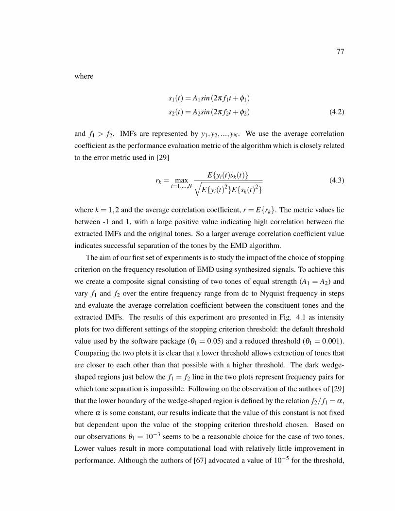
77
where
s1(t) = A1sin(2π f1t +ϕ1)
s2(t) = A2sin(2π f2t +ϕ2) (4.2)
and f1 > f2. IMFs are represented by y1,y2, ...,yN . We use the average correlation
coefficient as the performance evaluation metric of the algorithm which is closely related
to the error metric used in [29]
rk = maxi=1,...,N
Eyi(t)sk(t)√Eyi(t)
2Esk(t)2
(4.3)
where k = 1,2 and the average correlation coefficient, r = Erk. The metric values lie
between -1 and 1, with a large positive value indicating high correlation between the
extracted IMFs and the original tones. So a larger average correlation coefficient value
indicates successful separation of the tones by the EMD algorithm.
The aim of our first set of experiments is to study the impact of the choice of stopping
criterion on the frequency resolution of EMD using synthesized signals. To achieve this
we create a composite signal consisting of two tones of equal strength (A1 = A2) and
vary f1 and f2 over the entire frequency range from dc to Nyquist frequency in steps
and evaluate the average correlation coefficient between the constituent tones and the
extracted IMFs. The results of this experiment are presented in Fig. 4.1 as intensity
plots for two different settings of the stopping criterion threshold: the default threshold
value used by the software package (θ1 = 0.05) and a reduced threshold (θ1 = 0.001).
Comparing the two plots it is clear that a lower threshold allows extraction of tones that
are closer to each other than that possible with a higher threshold. The dark wedge-
shaped regions just below the f1 = f2 line in the two plots represent frequency pairs for
which tone separation is impossible. Following on the observation of the authors of [29]
that the lower boundary of the wedge-shaped region is defined by the relation f2/ f1 =α ,
where α is some constant, our results indicate that the value of this constant is not fixed
but dependent upon the value of the stopping criterion threshold chosen. Based on
our observations θ1 = 10−3 seems to be a reasonable choice for the case of two tones.
Lower values result in more computational load with relatively little improvement in
performance. Although the authors of [67] advocated a value of 10−5 for the threshold,
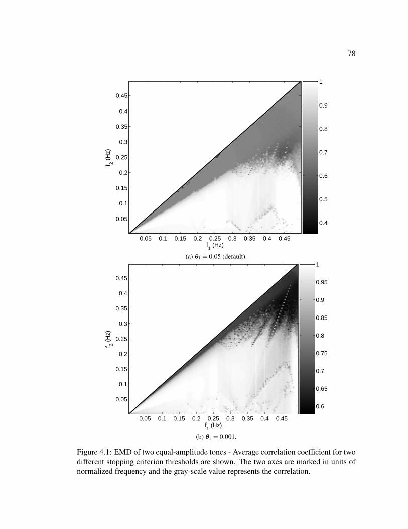
78
f1 (Hz)
f 2 (H
z)
0.05 0.1 0.15 0.2 0.25 0.3 0.35 0.4 0.45
0.05
0.1
0.15
0.2
0.25
0.3
0.35
0.4
0.45
0.4
0.5
0.6
0.7
0.8
0.9
1
(a) θ1 = 0.05 (default).
f1 (Hz)
f 2 (H
z)
0.05 0.1 0.15 0.2 0.25 0.3 0.35 0.4 0.45
0.05
0.1
0.15
0.2
0.25
0.3
0.35
0.4
0.45
0.6
0.65
0.7
0.75
0.8
0.85
0.9
0.95
1
(b) θ1 = 0.001.
Figure 4.1: EMD of two equal-amplitude tones - Average correlation coefficient for twodifferent stopping criterion thresholds are shown. The two axes are marked in units ofnormalized frequency and the gray-scale value represents the correlation.

79
1.2 1.4 1.6 1.8 2 2.2 2.4 2.6 2.8 30.7
0.75
0.8
0.85
0.9
0.95
f1/f
2
Ave
rage
cor
rela
tion
coef
ficie
nt
101005005000Defaultθ
1 = 0.001
Figure 4.2: EMD of two equal-amplitude tones - Average correlation coefficient is plot-ted against frequency ratio for different settings of maximum iteration limit and twodifferent stopping criterion thresholds.
while admitting that a value several orders of magnitude higher did not cause appreciable
loss of performance, we believe that similar level of performance can be achieved for
θ1 = 10−3 at much lower computational effort. Another aspect of the results that needs
mentioning is the fuzzy dark region in the right hand corner of the plots. To explain it
must be remembered that for EMD to be able to decompose a composite signal sufficient
amount of oversampling is required (a factor of five was suggested in [27]). So when
the two tones are close to each other and close to the Nyquist frequency, the algorithm
is unable to decompose them into separate IMFs resulting in a low correlation value.
The next set of simulations provide further insight into the relation between stopping
criterion and frequency resolution of EMD. The results presented in Fig. 4.2 show
the variation of the average correlation coefficient with frequency ratio for different
settings of maximum sifting iteration limit as well as stopping criterion threshold. It is
evident from the plot that more number of sifting iterations results in higher correlation
value for a particular frequency ratio thereby indicating better isolation of components.
The improvement in performance achieved by using a lower threshold for the stopping
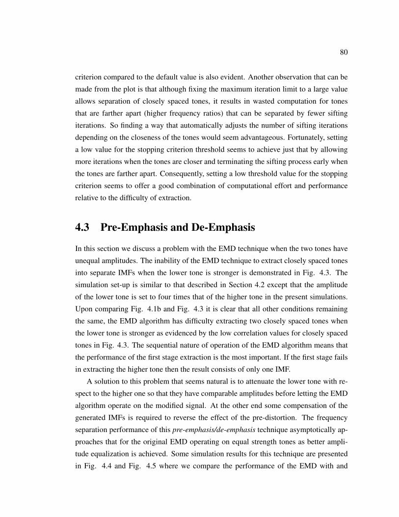
80
criterion compared to the default value is also evident. Another observation that can be
made from the plot is that although fixing the maximum iteration limit to a large value
allows separation of closely spaced tones, it results in wasted computation for tones
that are farther apart (higher frequency ratios) that can be separated by fewer sifting
iterations. So finding a way that automatically adjusts the number of sifting iterations
depending on the closeness of the tones would seem advantageous. Fortunately, setting
a low value for the stopping criterion threshold seems to achieve just that by allowing
more iterations when the tones are closer and terminating the sifting process early when
the tones are farther apart. Consequently, setting a low threshold value for the stopping
criterion seems to offer a good combination of computational effort and performance
relative to the difficulty of extraction.
4.3 Pre-Emphasis and De-Emphasis
In this section we discuss a problem with the EMD technique when the two tones have
unequal amplitudes. The inability of the EMD technique to extract closely spaced tones
into separate IMFs when the lower tone is stronger is demonstrated in Fig. 4.3. The
simulation set-up is similar to that described in Section 4.2 except that the amplitude
of the lower tone is set to four times that of the higher tone in the present simulations.
Upon comparing Fig. 4.1b and Fig. 4.3 it is clear that all other conditions remaining
the same, the EMD algorithm has difficulty extracting two closely spaced tones when
the lower tone is stronger as evidenced by the low correlation values for closely spaced
tones in Fig. 4.3. The sequential nature of operation of the EMD algorithm means that
the performance of the first stage extraction is the most important. If the first stage fails
in extracting the higher tone then the result consists of only one IMF.
A solution to this problem that seems natural is to attenuate the lower tone with re-
spect to the higher one so that they have comparable amplitudes before letting the EMD
algorithm operate on the modified signal. At the other end some compensation of the
generated IMFs is required to reverse the effect of the pre-distortion. The frequency
separation performance of this pre-emphasis/de-emphasis technique asymptotically ap-
proaches that for the original EMD operating on equal strength tones as better ampli-
tude equalization is achieved. Some simulation results for this technique are presented
in Fig. 4.4 and Fig. 4.5 where we compare the performance of the EMD with and
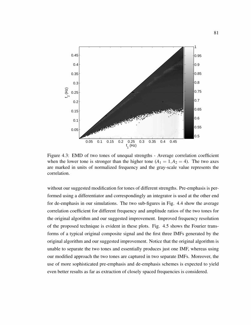
81
f1 (Hz)
f 2 (H
z)
0.05 0.1 0.15 0.2 0.25 0.3 0.35 0.4 0.45
0.05
0.1
0.15
0.2
0.25
0.3
0.35
0.4
0.45
0.5
0.55
0.6
0.65
0.7
0.75
0.8
0.85
0.9
0.95
1
Figure 4.3: EMD of two tones of unequal strengths - Average correlation coefficientwhen the lower tone is stronger than the higher tone (A1 = 1,A2 = 4). The two axesare marked in units of normalized frequency and the gray-scale value represents thecorrelation.
without our suggested modification for tones of different strengths. Pre-emphasis is per-
formed using a differentiator and correspondingly an integrator is used at the other end
for de-emphasis in our simulations. The two sub-figures in Fig. 4.4 show the average
correlation coefficient for different frequency and amplitude ratios of the two tones for
the original algorithm and our suggested improvement. Improved frequency resolution
of the proposed technique is evident in these plots. Fig. 4.5 shows the Fourier trans-
forms of a typical original composite signal and the first three IMFs generated by the
original algorithm and our suggested improvement. Notice that the original algorithm is
unable to separate the two tones and essentially produces just one IMF, whereas using
our modified approach the two tones are captured in two separate IMFs. Moreover, the
use of more sophisticated pre-emphasis and de-emphasis schemes is expected to yield
even better results as far as extraction of closely spaced frequencies is considered.

82
f1/f
2
A2/A
1
1.5 2 2.5 3
2
3
4
5
6
7
8
9
10
0.5
0.55
0.6
0.65
0.7
0.75
0.8
0.85
0.9
0.95
(a) Original EMD
f1/f
2
A2/A
1
1.5 2 2.5 3
2
3
4
5
6
7
8
9
10
0.3
0.4
0.5
0.6
0.7
0.8
0.9
(b) EMD + pre-emphasis/de-emphasis
Figure 4.4: EMD of two tones of unequal strengths - Performance comparison betweenthe original algorithm and the pre-emphasis and de-emphasis method. A differentiator-integrator pair is used for pre-emphasis and de-emphasis in this case. The gray-scalevalues represent the average correlation coefficients for each amplitude and frequencyratio pairs.
83
0.51
1.5
0
1
0
1Abs
olut
e F
FT
0 0.0625 0.125 0.1875 0.25 0.3125 0.375 0.4375 0.50
1
f (Hz)
(a) Original EMD
0.51
1.52
0
1
2
0
1
2
Abs
olut
e F
FT
0 0.0625 0.125 0.1875 0.25 0.3125 0.375 0.4375 0.50
1
2
f (Hz)
(b) EMD + pre-emphasis/de-emphasis
Figure 4.5: EMD of two tones of unequal strengths - Performance comparison betweenthe original algorithm and the pre-emphasis and de-emphasis method. The figures showthe Fourier transforms of a typical original composite signal and the first three IMFsgenerated by the respective techniques.
84
4.4 Conclusion
The newly developed empirical mode decomposition (EMD) technique has been applied
to many fields for signal analysis without a proper understanding its capabilities and lim-
itations. Further a clear understanding of how the simulation control parameters affect
its performance has eluded so far. In this work we have tried to answer some of these
questions. Using synthetic signals we have shown that more number of sifting iterations
results in better frequency isolation and have shown that setting the stopping criterion
threshold to a low value results in more sifting iterations and therefore better frequency
separation. Further we have pointed out the inability of this technique to separate two
tones when the lower tone is stronger and have offered a pre-emphasis/de-emphasis
technique to solve this problem. Simulation studies demonstrating the improvement in
performance due to the modification were presented. Although the poor frequency reso-
lution of the original EMD algorithm for certain signal condition is highlighted here and
a remedy introduced, the same improvement in performance can be realized in case of
RCEMD that also suffers poor frequency resolution for the same signal configuration.

Chapter 5
Overlay Communications using RaisedCosine Empirical Mode Decomposition
A signal overlay technique employing the empirical mode decomposition procedure is
presented here. A weak narrow-band signal is added to the primary signal that shares
the same frequency band. Careful signal design reduces interference caused to primary
users while ensuring successful recovery of the added signal. At the receiver a sta-
tionary filtering approach is ineffective in separating the signals because a fixed filter
designed to isolate one of the signals will also capture significant portion of the other
signal energy due to overlapping spectrums. However, the empirical mode decomposi-
tion technique, that isolates signal components based on their instantaneous frequencies,
is ideally suited to separate these time-varying signals with overlapping frequency com-
ponents. The choice of overlay signal transmission frequencies relative to that of the
primary signal is made in such a way that leads to greater resemblance of one of the
extracted components to the original overlay signal. An application to commercial fre-
quency modulation overlay is introduced initially with associated analysis and empirical
performance results. In the latter part of the chapter a covert communication technique
based on this overlay procedure is discussed and its performance analyzed. In addition
to the unique signal overlay structure discussed above, the covert technique employs
frequency-hopping and directional antenna to enhance signal covertness.
86
5.1 Introduction
Conventional communication systems are designed such that users are separated either
in the time, frequency, code or spatial domain. Traditional overlay systems involve over-
lap in the time and frequency domains, but the users are distinguishable due to distinct
codes or spatial positions. Here we describe a signal overlay procedure that involves
signal overlap in all four domains. Successful communication between different users
is possible due to distinct instantaneous frequencies (IF). We use the EMD algorithm to
separate users based on their IFs.
The EMD technique [27] provides an adaptive and efficient method to analyze non-
stationary signals. Here, overlay communications using the EMD technique is investi-
gated. We note that the tremendous growth in deployment of wireless technologies in
the past has led to a heavily utilized spectrum with most frequency bands already as-
signed to licensed (primary) users for specific services. Although cognitive radio tech-
nology [84] admits co-existence of multiple radio signals within the same frequency
band, identifying and utilizing spectral holes are challenging issues.
In this chapter a signal overlay technique employing EMD is presented to improve
spectrum utilization. A primary, licensed user of the frequency band is considered here.
In this work a frequency modulated (FM) signal is considered as the primary signal.
A secondary transmitter that is not necessarily co-located with the primary transmitter
transmits another signal in the same frequency band. The secondary signal is weak and
narrow-band relative to the primary signal. Due to the weak nature of the secondary
signal, primary users of the frequency band experience negligible interference. At the
same time, due to careful signal design, the secondary receiver is able to extract the
secondary signal using the EMD procedure from the composite signal present at its
input.
Traditionally, signal overlay involves spreading the transmission bandwidth of the
secondary signal so that its power spectral density is less than that of noise to eliminate
interference to the primary user. Strategies that make this possible include the direct-
sequence spread spectrum (DSSS) and ultra-wideband (UWB) signalling techniques
( [85] describes a DSSS overlay system). Due to the large transmission bandwidths
associated with these techniques, the primary user’s signal appears as narrow-band in-
terference (NBI) to the secondary user. For DSSS signals two classes of interference
87
rejection techniques are used for general NBI: those based upon least-mean square esti-
mation techniques, and those following transform domain processing principles [86,87].
Further, [88–91] describe DSSS overlay systems where the NBI is an angle-modulated
signal, specifically an FM signal. Narrowband interference rejection techniques in UWB
systems generally follow space-time receiver strategies [92–94]. In contrast to the pre-
ceding techniques that require a wideband secondary signal, the proposed technique
involves transmission of a narrowband secondary signal occupying a portion of the pri-
mary signal spectrum. Primary users experience negligible interference due to the added
signal because of its small relative power. A specific configuration of the secondary
signal relative to the primary, based on their frequencies, that leads to successful de-
composition using EMD is described here. This choice of frequencies, that is crucial
for successful signal extraction, exploits the unique properties of the EMD procedure.
Moreover, traditional nonstationary filtering techniques are ineffective in separating the
signals due to their overlapping IFs. To summarize, the essential attributes of the pro-
posed technique are as follows:
• The primary and secondary users overlap in the spatial domain.
• Simultaneous overlap in the time and frequency domains is also assumed.
• The two signals are have distinct IFs most of the time and are therefore separable
by an appropriate technique that exploits this property.
• Fixed filters are ineffective in separating the signals due to overlapping IFs, since
they have fixed pass- and stop-bands.
• A time-frequency approach that isolates the signals based on their IFs is required
for signal separation.
Specific design considerations and performance results for this new technique are
presented in the following sections. Section 5.2 describes this signal overlay technique
in greater detail and also gives a brief overview of the EMD procedure that is crucial for
successful signal extraction. Section 5.3 addresses performance issues of this commu-
nication scheme and introduces an analytical performance measure. Simulation results
are discussed in Section 5.4. A complex-valued version of this algorithm is introduced
in Section 5.5 while Section 5.7 presents some concluding remarks.
88
5.2 Signal Design
The simultaneous transmission of a weak secondary signal in the same frequency band
of a primary user and its subsequent extraction is the objective of this work. The small
power level of the secondary signal guarantees negligible additional interference to the
primary user. This new technique is illustrated using an example of a weak frequency
shift keying (FSK) signal superimposed on a FM broadcast signal. Despite the apparent
similarity to cognitive radio technology, the proposed technique has a crucial differ-
ence: the secondary transmitter in the proposed technique transmits continuously, and
therefore does not require spectrum sensing to identify holes. The secondary receiver
performs EMD on the received signal (FM + FSK) to generate a series of elementary
signal components, one of which corresponds to the transmitted FSK signal with high
probability.
The EMD technique decomposes the multicomponent signal into its constituents
solely based upon the IFs present at any particular time and the relative amplitudes of
the components (an analysis of the signal separation abilities of EMD as a function of
relative amplitudes of the components is presented in [61] for the specific case of two-
tone signals). When the signal components satisfy certain conditions on the ratio of their
IFs and their relative amplitudes, they can be extracted into distinct IMFs. However,
when the IFs of the components intersect, the signal decomposition algorithm fails to
extract the components into distinct IMFs and portions of each signal component are
spread over several IMFs. The effect of this phenomenon, that is sometimes referred to
as mode splitting in literature, on our proposed technique is examined in Section 5.3.1.
The choice of secondary signal frequency relative to the primary is based on the
properties of the EMD algorithm. The choice is mainly influenced by two factors: one,
that the secondary signal has a smaller amplitude relative to the primary to reduce inter-
ference to the users of the primary signal, and, second, that signal decomposition quality
using EMD depends on the amplitude ratio of the signal components; higher quality re-
sulting when the stronger component has a larger IF [44, 61]. Consequently, the choice
of secondary signal frequencies is such that the IF of the secondary signal is smaller
than that of the primary signal with high probability. In practice, this is accomplished
by choosing frequencies near the lower edge of the FM band to insert the secondary
signal.

89
nrsLPF EMD
r′p + r′s + n′rp + rs + n
rp
fFM − fIFigure 5.1: Block diagram of the secondary receiver.
Formally, the combined signal as seen by the primary and secondary receivers may
be represented as
r′(t) = r′p(t)+ r′s(t)+n′(t) (5.1)
where r′p(t) and r′s(t) represent the primary and the superimposed secondary signals
respectively and n′(t) is the additive white Gaussian noise (AWGN) with power spectral
density N0 Watts/Hz. The secondary transmitter and receiver are located within the
FM broadcast region. The maximum separation between the two is determined by the
maximum overlay signal strength that can be transmitted without causing noticeable
interference to nearby FM receivers and by the maximum allowable bit-error-rate (BER)
at the overlay receiver. A more thorough discussion on these constraints is presented in
the following sections. At the secondary receiver, the combined FM broadcast plus FSK
signal having a bandwidth of B Hz is first frequency shifted to a range of 0−B Hz,
generating a complex-valued signal. The EMD procedure is then applied to the down-
converted signal to extract the secondary signal. Figure 5.1 shows the block diagram of
the secondary receiver. In this case, fFM is the center frequency of the commercial FM
band and the intermediate frequency, fI = B/2 Hz. After down-conversion the complex-
valued signals are denoted in the same fashion as in (5.1), but without the primes. The
validity of the technique is demonstrated by applying real-valued EMD algorithm to the
composite signal in the following two sections. Section 5.5 introduces the complex-
valued algorithm.
The reason for the frequency down-conversion step follows. As pointed out in [61,
95] in the context of separation of pure tones of frequencies f1 and f2 ( f1 > f2), the
quality of extraction depends upon the ratio f1/ f2. A larger frequency ratio for a given
amplitude ratio results in better signal decomposition quality. By down-converting the
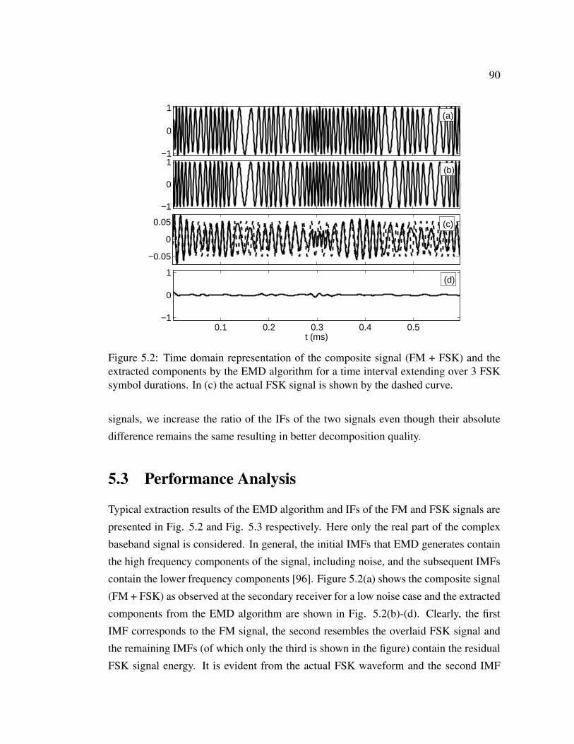
90
−1
0
1
−1
0
1
−0.05
0
0.05
0.1 0.2 0.3 0.4 0.5−1
0
1
t (ms)
(a)
(b)
(c)
(d)
Figure 5.2: Time domain representation of the composite signal (FM + FSK) and theextracted components by the EMD algorithm for a time interval extending over 3 FSKsymbol durations. In (c) the actual FSK signal is shown by the dashed curve.
signals, we increase the ratio of the IFs of the two signals even though their absolute
difference remains the same resulting in better decomposition quality.
5.3 Performance Analysis
Typical extraction results of the EMD algorithm and IFs of the FM and FSK signals are
presented in Fig. 5.2 and Fig. 5.3 respectively. Here only the real part of the complex
baseband signal is considered. In general, the initial IMFs that EMD generates contain
the high frequency components of the signal, including noise, and the subsequent IMFs
contain the lower frequency components [96]. Figure 5.2(a) shows the composite signal
(FM + FSK) as observed at the secondary receiver for a low noise case and the extracted
components from the EMD algorithm are shown in Fig. 5.2(b)-(d). Clearly, the first
IMF corresponds to the FM signal, the second resembles the overlaid FSK signal and
the remaining IMFs (of which only the third is shown in the figure) contain the residual
FSK signal energy. It is evident from the actual FSK waveform and the second IMF

91
0 0.2 0.4 0.6 0.8 120
40
60
80
100
120
140
160
180
t (ms)
Inst
anta
neou
s fr
eque
ncy
(kH
z)
Figure 5.3: Instantaneous frequencies of the FM signal (solid) and the FSK signal(dashed) for a time interval extending over 5 FSK symbol durations. The hatched areaindicates the times when signal decomposition is not possible.
in Fig. 5.2(c) that although the second IMF closely approximates the original signal
over certain intervals, at other times it deviates from the original due to superimposed
amplitude and frequency modulations.
The superimposed amplitude modulated (AM) signal and the newly introduced fre-
quencies in the second IMF can be explained based on the IFs of the two signals, shown
in Fig. 5.3. For an FM signal represented by
rp(t) = Apcos
2π fIt + k f
t∫−∞
m(τ)dτ
(5.2)
the IF is given by [97]
finst = fI +k f
2πm(t) (5.3)
where k f represents the frequency-deviation constant (bandwidth of the FM signal is
directly proportional to k f ), m(t) is the modulating/information signal and Ap is the
92
amplitude of the FM signal. This IF is shown in Fig. 5.3 for an arbitrary modulating
signal. The IF of the FSK signal is also shown in the figure. Due to the intersecting
IFs, common nonstationary signal decomposition techniques result in poor signal de-
composition quality. However, using the EMD procedure, when the IF of the primary
signal is significantly larger than that of the secondary signal, extraction is successful
and high fidelity separation of the signal components into different IMFs occurs. When
the primary signal’s IF is either close to that of the secondary signal or smaller, the
EMD extraction fails to produce an IMF that contains a useful copy of the FSK signal.
The algorithm fills the interval with a signal having smoothly varying amplitude and
random frequency to maintain phase continuity with the correctly extracted portion of
the secondary signal. The affected intervals are shown by the hatched area in Fig. 5.3.
To avoid this phenomenon, the overlay FSK frequencies are chosen such that they are
smaller than the IFs of the primary signal with high probability. Thus, frequencies near
the lower edge of frequency band of the primary signal are selected for transmitting the
secondary signal. Moreover, the EMD algorithm is more effective in signal separation
when the stronger signal has a larger IF [44].
5.3.1 Choice of decomposition level
The number of IMFs generated in the overlay receiver are in concordance with the sig-
nal overlay design presented in the previous section. For small Eb/N01, mode splitting,
i.e., the distribution of the constituent signal components across multiple IMFs, is likely
and reconstituting the secondary FSK signal for detection is intractable. In short, for
small Eb/N0 the error rate is large regardless of the number of IMFs generated. For
larger Eb/N0, the EMD reliably separates the overlay FSK signal into the second and
subsequent IMFs. We see experimentally that the second IMF produces the highest fi-
delity representation of the FSK signal, however, smaller residuals of the FSK signal
may still appear in higher order IMFs if they are generated. Thus, the overlay FSK
receiver only generates the first two IMFs and always uses the second IMF for FSK
detection. This approach has a two-fold advantage. First, it improves error rate perfor-
mance over a higher-order decomposition because it does not permit the FSK signal to
distribute among multiple IMFs. Second, it reduces the receiver complexity since only
1Eb/N0 is a measure of the signal-to-noise-ratio (SNR), also known as SNR per bit, and is a commonlyused metric in communication literature.

93
two IMFs are generated and IMF selection is not an issue. We can track the perfor-
mance degradation when the overlay receiver generates and uses more than two IMFs
from that presented in Section 5.4 (Fig. 5.11). Taking BER=10−2 as a reference, the
overlay receiver loses 2 dB if it generates all IMFs and uses the one with the largest de-
cision statistic for detection. The overlay receiver loses 3 dB if it generates all IMFs and
always uses the second IMF for detection. Both of these alternate approaches only use
a portion of the FSK signal for detection. This assertion is further validated when the
overlay receiver attempts to collect the FSK signal by using the sum of the second and
third IMFs, which results in small fractions of a decibel degradation from that shown in
Fig. 5.11.
5.3.2 Performance approximation
Here we develop a model for the extracted secondary signal using EMD that leads to
a simple formula for the resulting BER performance. Based on the above discussion,
it is clear that second IMF generated by the algorithm is a high fidelity approximation
of the original FSK signal over the interval when the IF of the FM signal exceeds that
of the FSK signal, and has little resemblance to the transmitted signal when the order
of the IFs gets reversed. So corresponding to the two conditions we model the second
IMF either as an exact copy of the transmitted FSK signal or as a signal with random
frequency and amplitude over the respective intervals. As a result, the cross-correlation
coefficient between the segments of the second IMF containing random frequencies and
the original FSK signal is zero, on average. To model this, we represent by T1 and T2
the average amount of time within an FSK bit interval, T , that the two FSK frequencies
are larger than the FM IF, finst . The secondary BER can then be derived by suitably
adjusting the Eb/N0 value in the standard non-coherent FSK result to reflect the fraction
of the total signal energy that is useful in FSK detection. Then the resulting BER for
non-coherent FSK is
Pb =12
e− 1
2
(EbN0
)e f f (5.4)
where (Eb
N0
)e f f
=Eb
N0(1−ξ ) (5.5)

94
where ξ = T1+T2T is the fraction of time when the FSK IF is larger than finst . As a result,
(1−ξ ) represents the fraction of the signal energy that contributes to successful symbol
detection. The BER derived from this simple model and simulation results are shown in
Section 5.4 (Fig. 5.6), where close agreement is observed.
Analyzing the system performance based on the relative IFs of the two signals as
described above provides insight into the working of the technique, thereby allowing a
judicious choice of secondary signal transmission frequencies. It is clear that choosing
the FSK transmission frequencies near the upper and lower bounds of the FM IF range
results in maximum and minimum duration of unfavorable IF configuration, correspond-
ing to the largest and smallest error in the extracted signals using EMD, respectively for
a given Eb/N0 (See Fig. 5.3). Therefore, the minimum IF attained by the FM signal
determines the smallest FSK transmission frequency in this technique. In practical sit-
uations, the FM modulating signal amplitude bears a linear relationship to its IF and
ultimately determines the duration over which the EMD algorithm fails to correctly de-
compose the two signals. Due to the statistical nature of the modulating signal, it is
simulated using a stochastic model for performance verification in Section 5.4.
5.4 Simulation Results
FSK BER and FM normalized mean-squared-error (NMSE) for the overlay technique
using EMD are presented in Fig. 5.11 and Fig. 5.5 respectively. The NMSE for FM
signal, ε , is defined as
ε =∥rp − v1(t)∥
∥rp∥(5.6)
where v1(t) represents the first IMF and ∥.∥ indicates the L2 norm defined for a function
f (x) as follows
∥ f (x)∥=(∫
| f (x)|2dx)1/2
.
Since only two IMFs are generated in our technique, the second IMF, v2(t) is used for
FSK detection. The drop in BER and NMSE values at large Eb/N0 indicates that the
two signals are successfully separated into the intended IMFs, as discussed in Section
5.3. For these results, the received FSK signal was 26 dB weaker than the FM signal.
Also, secondary data transmission rate of 5 kbps was simulated and an over-sampling

95
2 4 6 8 10 12 14 16 18 20
10−4
10−3
10−2
10−1
100
Eb/N
0 (dB)
BE
R
EMDWVDAFRemod
Figure 5.4: Eb/N0-vs-BER plots for the signal overlay scheme. Performance of theproposed technique is compared with that of the Wigner-Ville distribution (WVD)-basedtechnique and the adaptive filter (AF) technique.
factor of 10 was employed due to dense sampling requirement of EMD for accurate
determination of local extrema, as discussed in Section 5.2. So, voice communications
and low-rate data communications using error-correcting codes are possible applications
of this overlay scheme. The FM modulating signal in our experiments is generated using
a general stochastic time-varying model, namely a first-order auto-regressive (AR(1))
model. The choice of low-order filter-model is based on our experimental observation
that the proposed technique is insensitive to the model-order used for signal generation
for the same signal bandwidth.
In Fig. 5.11 BER performance results for three alternate techniques are also pre-
sented. The first method is a two-step procedure where the IF of the FM signal is first
estimated using the Wigner-Ville distribution (WVD) and then a short, time-varying fi-
nite impulse response (FIR) notch filter is designed to remove that frequency [88]. The
time-varying nature of the primary signal requires a short length notch filter, which cor-
responds to a wide notch in the frequency domain, thereby significantly distorting the
secondary signal. In the original scenario in [88] since the interference (FM) signal oc-
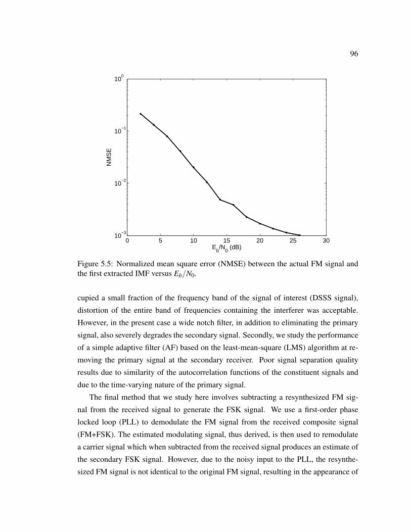
96
0 5 10 15 20 25 3010
−3
10−2
10−1
100
Eb/N
0 (dB)
NM
SE
Figure 5.5: Normalized mean square error (NMSE) between the actual FM signal andthe first extracted IMF versus Eb/N0.
cupied a small fraction of the frequency band of the signal of interest (DSSS signal),
distortion of the entire band of frequencies containing the interferer was acceptable.
However, in the present case a wide notch filter, in addition to eliminating the primary
signal, also severely degrades the secondary signal. Secondly, we study the performance
of a simple adaptive filter (AF) based on the least-mean-square (LMS) algorithm at re-
moving the primary signal at the secondary receiver. Poor signal separation quality
results due to similarity of the autocorrelation functions of the constituent signals and
due to the time-varying nature of the primary signal.
The final method that we study here involves subtracting a resynthesized FM sig-
nal from the received signal to generate the FSK signal. We use a first-order phase
locked loop (PLL) to demodulate the FM signal from the received composite signal
(FM+FSK). The estimated modulating signal, thus derived, is then used to remodulate
a carrier signal which when subtracted from the received signal produces an estimate of
the secondary FSK signal. However, due to the noisy input to the PLL, the resynthe-
sized FM signal is not identical to the original FM signal, resulting in the appearance of

97
2 4 6 8 10 12 14 16 18
10−4
10−3
10−2
10−1
100
Eb/N
0 (dB)
BE
R
FSK BER (Sim.)FSK BER (Anal.)
Figure 5.6: Eb/N0-vs-BER plot using the proposed signal extraction technique. BERvalues derived from theory (Equation 5.4) and those obtained from simulation for arange of Eb/N0 are shown.
some FM signal energy in the difference. Figure 5.7 shows the block diagram for this
receiver. It is observed from Fig. 5.8 that the BER for this remodulation technique satu-
rates for large Eb/N0 because the residual phase error at PLL output due to noisy input
(FM+FSK+thermal noise) is essentially limited by the FSK signal amplitude, which is
independent of Eb/N0. To validate the performance result of the PLL technique obtained
from simulations, we followed a semi-analytical method to study the performance. Here,
the response of the PLL due to noisy input is modeled as random phase error of certain
level [98]. The detected signal including the random phase error is then used to resyn-
thesize the FM signal as described above. The BER of the FSK signal resulting from
this semi-analytical method and that obtained from simulating a PLL are shown in Fig.
5.8 for a range of Eb/N0 values. The closeness of the two plots validates our results.

98
FMDemodulator(PLL)
FMModulator
mrp + rs + n
+−
rp rs + n
Delay
fFM
Figure 5.7: Block diagram of the receiver using remodulation technique.
5.4.1 Effect on primary users
To analyze the effect of the secondary signal on the users of the primary signal we note
that at any instant the FSK signal appears as a tone interferer to the FM receiver. It has
been shown that the output of an ideal frequency demodulator due to a tone interferer is
given by [97]
ys(t) =As
Ap2π( fI − fk)cos(2π( fI − fk)t) (5.7)
where k = 1, 2 corresponding to the two FSK frequencies and Ap and As are the am-
plitudes of the primary and secondary signals respectively, with As ≪ Ap. Since the
interference output is inversely proportional to the primary signal amplitude, the weak
interference is suppressed and so the interference level must be at least 6 dB weaker
than the FM signal to avoid objectionable interference to the FM listener [97]. To quan-
tify the distortion caused at the output of an ideal frequency demodulator due to the
combined effect of the secondary (FSK) signal and background noise, we introduce a
measure
η =∥m(t)−m(t)∥2
∥m(t)∥2 (5.8)
where ∥.∥ indicates the L2 norm as discussed earlier and m(t) is the estimate of mod-
ulating signal, m(t) produced by the ideal frequency demodulator. Simulation results
indicate that the additional distortion introduced due to insertion of the secondary sig-
nal is less than 2 dB more than that caused by background noise alone for the entire of
range of secondary signal and noise levels shown in Fig. 5.11. This distortion is small

99
0 5 10 15 20 25 3010
−2
10−1
100
Eb/N
0 (dB)
BE
R
PLL (Order 1)Added phase noise
Figure 5.8: Comparison of FSK BER derived from simulation of PLL and semi-analytical method that models the phase error at the PLL output. Similar results fromthe two techniques is evident.
at low values of Eb/N0 where the effect of background noise is strong, but increases at
large values of Eb/N0 when the effect of the added secondary signal dominates. Also,
our studies indicate that any possible aliasing due to frequency down-conversion has
negligible effect on the performance, implying that this technique is not alias-limited.
5.5 Operations on the Complex Baseband Signal
So far we have considered only real-valued signals for secondary signal detection using
EMD. However, it is possible to further reduce the error rate by exploiting the informa-
tion available in the in-phase and quadrature-phase components of the baseband signal
as a whole. In this section we will quantify the performance improvement realized by
utilizing the inherent symmetry of the complex signal components.
A logical way to extend the EMD technique to the complex domain is to indepen-
dently apply the algorithm to the two signal components, and thereafter computing the
log-likelihood ratio (LLR) corresponding to each FSK bit. The final bit decisions are

100
2 4 6 8 10 12 14 16 18
10−4
10−3
10−2
10−1
100
Eb/N
0 (dB)
BE
R
BER, realBER, cmplx.BER, BEMD
Figure 5.9: Eb/N0-vs-BER graph showing performance improvement offered by per-forming signal decomposition on the complex signal.
based on the combined LLR. This represents an straight-forward way to apply the EMD
algorithm to complex signals.
The bivariate EMD algorithm [55] (which is a generalization of the algorithm in-
troduced in [56]) is an extension of the original EMD algorithm to the complex do-
main. This algorithm operates on complex-valued signals, generating bivariate IMFs.
Applied to complex-valued signals, slow oscillations are extracted as the mean of a
three-dimensional envelope enclosing the signal. This envelope is computed by con-
sidering a fixed number of directions: the signal is projected in each direction and an
envelope is computed for each of these real-valued signals using the original EMD pro-
cedure. Projecting these envelopes back into the complex domain defines the shape
of the three-dimensional envelope at each time instant. Higher fidelity definition of
the three-dimensional envelope due to more numerous projecting directions has been
claimed [55]. The mean of this envelope is analogous to the mean signal derived using
classical EMD.
We next consider the achievable performance for the overlay technique when the
complex-valued baseband signal is decomposed. Figure 5.9 shows these results. Two
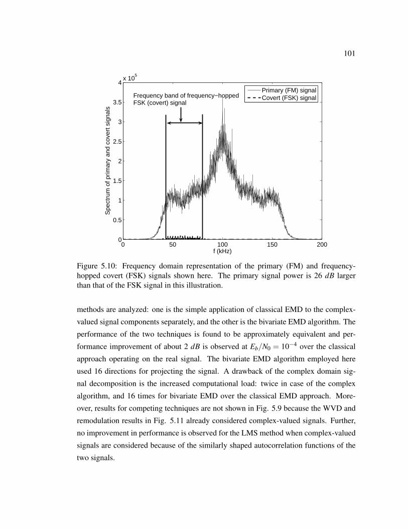
101
0 50 100 150 2000
0.5
1
1.5
2
2.5
3
3.5
4x 10
5
f (kHz)
Spe
ctru
m o
f prim
ary
and
cove
rt s
igna
ls
Primary (FM) signalCovert (FSK) signalFrequency band of frequency−hopped
FSK (covert) signal
Figure 5.10: Frequency domain representation of the primary (FM) and frequency-hopped covert (FSK) signals shown here. The primary signal power is 26 dB largerthan that of the FSK signal in this illustration.
methods are analyzed: one is the simple application of classical EMD to the complex-
valued signal components separately, and the other is the bivariate EMD algorithm. The
performance of the two techniques is found to be approximately equivalent and per-
formance improvement of about 2 dB is observed at Eb/N0 = 10−4 over the classical
approach operating on the real signal. The bivariate EMD algorithm employed here
used 16 directions for projecting the signal. A drawback of the complex domain sig-
nal decomposition is the increased computational load: twice in case of the complex
algorithm, and 16 times for bivariate EMD over the classical EMD approach. More-
over, results for competing techniques are not shown in Fig. 5.9 because the WVD and
remodulation results in Fig. 5.11 already considered complex-valued signals. Further,
no improvement in performance is observed for the LMS method when complex-valued
signals are considered because of the similarly shaped autocorrelation functions of the
two signals.
102
5.6 Covert Communications using Empirical Mode De-
composition
Covert communication has traditionally involved either spreading the bandwidth over
which the signal is transmitted so that its power spectral density is smaller than that of
noise or changing the carrier frequency of the signal rapidly to avoid detection. Develop-
ments in this area have given rise to the whole field of transmission security (TRANSEC)
that deals with signals possessing low probability of detection (LPD), low probability of
interception (LPI), low probability of exploitation (LPE) and anti-jam (AJ) features [99].
In some situations it may be useful to hide the presence or existence of the communica-
tor’s signal. Traditionally, this has meant that at an unintended receiver, the communi-
cated signal plus receiver noise and interference cannot be reliably distinguished from
just receiver noise plus interference. Therefore, LPD signals refer to those that make it
difficult for unintended receivers to detect them.
Here we propose a LPD signal design strategy that aims to hide the signal un-
der a stronger primary signal corresponding to an existing legitimate communication
or broadcast service. The covert signal design ensures that it is undetectable by pri-
mary users while at the same time allows reliable recovery at the covert receiver. This
concept is demonstrated here using an example of a covert transceiver on the ground
communicating with an aerial vehicle using a weak narrow-band signal. This signal is
superimposed on an existing primary signal that is analogous to a cover signal. The
covert receiver, at the other end, receives the composite (primary + covert) signal and
extracts the weak covert signal by performing signal decomposition using RCEMD [95].
Distinct spatial positions and codes between the primary and covert users can be addi-
tionally used to improve the performance of the technique in terms of achievable data
rate or communication range. This is achieved by the use of directional antenna by the
covert transmitter to reduce the observable covert signal power by the primary receivers
on the ground. Frequency hopping (FH) is also introduced to make signal detection by
the unintended receiver more difficult. Further, no cooperation is assumed between the
primary and covert signal transmissions and this technique does not depend upon the
presence of spectral nulls in the stronger primary signal for successful communication.
The signal design for covert communications is similar to the earlier case of overlay
communications, involving commercial FM broadcast signal as the primary (cover) sig-
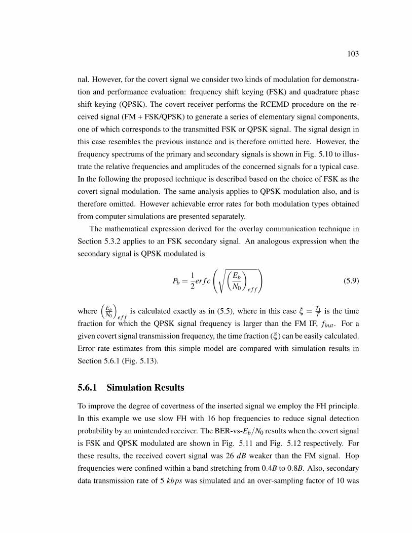
103
nal. However, for the covert signal we consider two kinds of modulation for demonstra-
tion and performance evaluation: frequency shift keying (FSK) and quadrature phase
shift keying (QPSK). The covert receiver performs the RCEMD procedure on the re-
ceived signal (FM + FSK/QPSK) to generate a series of elementary signal components,
one of which corresponds to the transmitted FSK or QPSK signal. The signal design in
this case resembles the previous instance and is therefore omitted here. However, the
frequency spectrums of the primary and secondary signals is shown in Fig. 5.10 to illus-
trate the relative frequencies and amplitudes of the concerned signals for a typical case.
In the following the proposed technique is described based on the choice of FSK as the
covert signal modulation. The same analysis applies to QPSK modulation also, and is
therefore omitted. However achievable error rates for both modulation types obtained
from computer simulations are presented separately.
The mathematical expression derived for the overlay communication technique in
Section 5.3.2 applies to an FSK secondary signal. An analogous expression when the
secondary signal is QPSK modulated is
Pb =12
er f c
(√(Eb
N0
)e f f
)(5.9)
where(
EbN0
)e f f
is calculated exactly as in (5.5), where in this case ξ = T1T is the time
fraction for which the QPSK signal frequency is larger than the FM IF, finst . For a
given covert signal transmission frequency, the time fraction (ξ ) can be easily calculated.
Error rate estimates from this simple model are compared with simulation results in
Section 5.6.1 (Fig. 5.13).
5.6.1 Simulation Results
To improve the degree of covertness of the inserted signal we employ the FH principle.
In this example we use slow FH with 16 hop frequencies to reduce signal detection
probability by an unintended receiver. The BER-vs-Eb/N0 results when the covert signal
is FSK and QPSK modulated are shown in Fig. 5.11 and Fig. 5.12 respectively. For
these results, the received covert signal was 26 dB weaker than the FM signal. Hop
frequencies were confined within a band stretching from 0.4B to 0.8B. Also, secondary
data transmission rate of 5 kbps was simulated and an over-sampling factor of 10 was
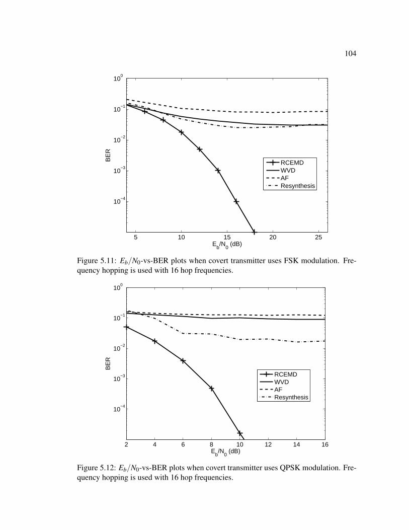
104
5 10 15 20 25
10−4
10−3
10−2
10−1
100
Eb/N
0 (dB)
BE
R
RCEMDWVDAFResynthesis
Figure 5.11: Eb/N0-vs-BER plots when covert transmitter uses FSK modulation. Fre-quency hopping is used with 16 hop frequencies.
2 4 6 8 10 12 14 16
10−4
10−3
10−2
10−1
100
Eb/N
0 (dB)
BE
R
RCEMDWVDAFResynthesis
Figure 5.12: Eb/N0-vs-BER plots when covert transmitter uses QPSK modulation. Fre-quency hopping is used with 16 hop frequencies.

105
2 4 6 8 10 1210
−7
10−6
10−5
10−4
10−3
10−2
10−1
Eb/N
0 (dB)
BE
R
QPSK BER (Simul.)QPSK BER (Theor.)
Figure 5.13: Cross-validation of error rate performance derived from simple numeri-cal model (Equation 5.9) and computer simulation output for QPSK modulated covertsignal. Ratio of primary to covert signal power is 26 dB here.
employed. So, voice communications and low-rate data communications using error-
correcting codes are possible applications of this overlay scheme. For our experiments
the FM modulating signal is modeled as a filtered noise output of a first-order auto-
regressive (AR(1)) model.
In Fig. 5.11 and Fig. 5.12 BER performance results for three alternate techniques
are also presented. The first method is a two-step procedure where the IF of the FM
signal is first estimated using the Wigner-Ville distribution (WVD) and then a short,
time-varying finite impulse response (FIR) notch filter is designed to remove that fre-
quency [88]. The time-varying nature of the primary signal requires a short length notch
filter, which corresponds to a wide notch in the frequency domain, thereby significantly
distorting the secondary signal. In the original scenario in [88] since the interference
(FM) signal occupied a small fraction of the frequency band of the signal of interest
(DSSS signal), distortion of the entire band of frequencies containing the interferer was
negligible. However, in the present case a wide notch filter, in addition to eliminating
the primary signal, also severely degrades the secondary signal. Secondly, we study
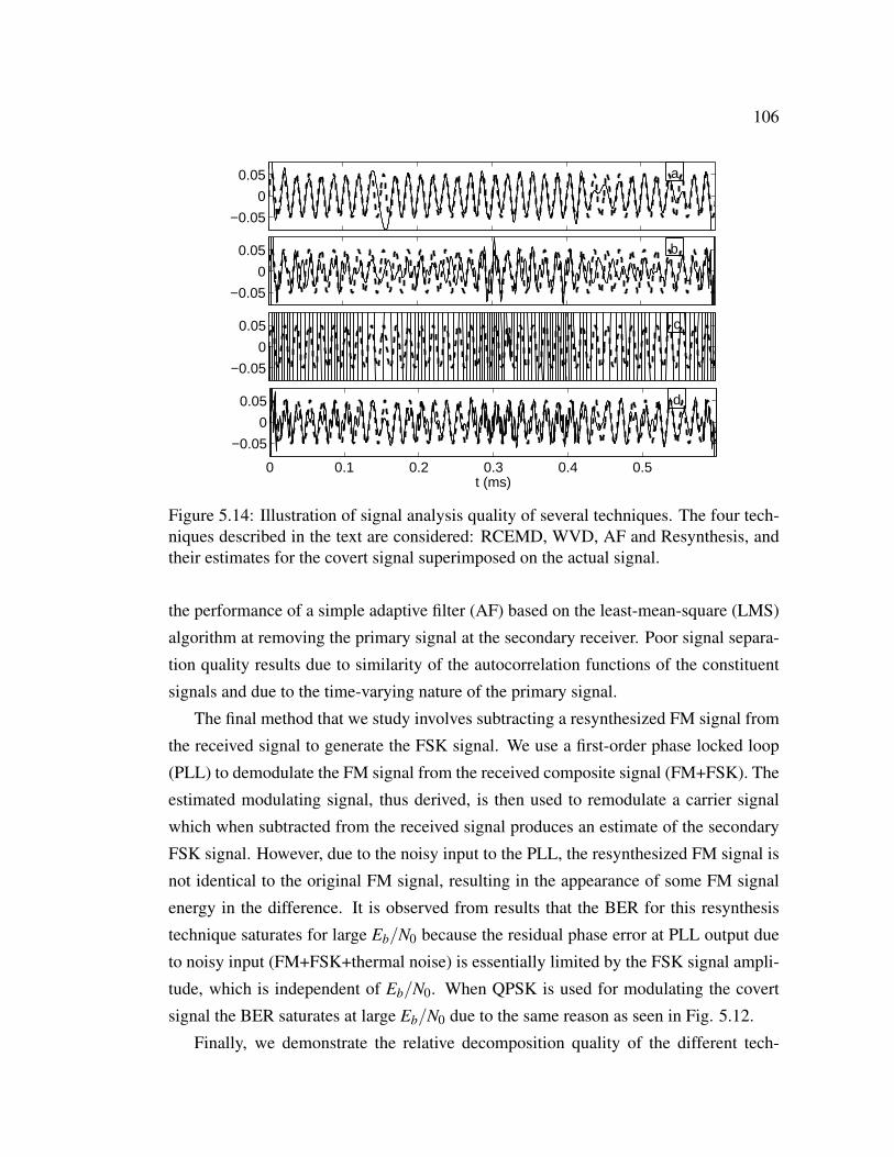
106
−0.05
0
0.05
−0.05
0
0.05
−0.05
0
0.05
0 0.1 0.2 0.3 0.4 0.5
−0.05
0
0.05
t (ms)
a
b
c
d
Figure 5.14: Illustration of signal analysis quality of several techniques. The four tech-niques described in the text are considered: RCEMD, WVD, AF and Resynthesis, andtheir estimates for the covert signal superimposed on the actual signal.
the performance of a simple adaptive filter (AF) based on the least-mean-square (LMS)
algorithm at removing the primary signal at the secondary receiver. Poor signal separa-
tion quality results due to similarity of the autocorrelation functions of the constituent
signals and due to the time-varying nature of the primary signal.
The final method that we study involves subtracting a resynthesized FM signal from
the received signal to generate the FSK signal. We use a first-order phase locked loop
(PLL) to demodulate the FM signal from the received composite signal (FM+FSK). The
estimated modulating signal, thus derived, is then used to remodulate a carrier signal
which when subtracted from the received signal produces an estimate of the secondary
FSK signal. However, due to the noisy input to the PLL, the resynthesized FM signal is
not identical to the original FM signal, resulting in the appearance of some FM signal
energy in the difference. It is observed from results that the BER for this resynthesis
technique saturates for large Eb/N0 because the residual phase error at PLL output due
to noisy input (FM+FSK+thermal noise) is essentially limited by the FSK signal ampli-
tude, which is independent of Eb/N0. When QPSK is used for modulating the covert
signal the BER saturates at large Eb/N0 due to the same reason as seen in Fig. 5.12.
Finally, we demonstrate the relative decomposition quality of the different tech-

107
5 10 15 2010
−1
100
Eb/N
0 (dB)
NM
SE
RCEMDWVDAFResynthesis
Figure 5.15: Numerical comparison of decomposition quality for several techniques ispresented here. The normalized mean squared error between the actual and estimatedcovert signal is shown for four algorithms described in text.
niques introduced above. Figure 5.14 presents the estimate of the covert signal obtained
using the four methods considered in this chapter, superimposed on the original covert
signal. Although severe distortion due to the AF technique is evident, the RCEMD,
WVD and Resynthesis results appear better, with the RCEMD output resembling the
original signal the most. A quantitative measure of the decomposition quality is shown
in Fig. 5.15, where the normalized mean-squared-error (NMSE) between the extracted
components using different techniques and the original signal is presented for varying
Eb/N0.
5.6.2 Communication Range Determination
The maximum communication range for the covert users is limited by two constraints.
The minimum SNR required at the covert receiver for reliable signal detection is one
constraint. Large transmit power is desirable in this case. The other requirement is
that users of the primary signal in the vicinity of the covert transmitter be unaffected
by the inserted signal. This requires small transmit power. It is evident that the two

108
0.5 1 1.5 2 2.5 3 3.5 4 4.5 5
50
100
150
200
250
300
350
Distance of covert transmitter from FM tower (km)
Max
imum
ran
ge o
f aer
ial v
ehic
le (
km)
FSKQPSK
Figure 5.16: Maximum achievable range for the covert communication technique isshown here. The plotted horizontal ranges of the aerial vehicle are the maximum possi-ble to ensure BER < 10−5 for the respective modulation types.
requirements place opposing constraints on the transmit signal power. To calculate the
useful communication range for this technique we first find that largest allowable trans-
mit power for the covert user that allows normal signal reception by nearby primary
users and then find the maximum range at which the covert receiver can be located for
reliable signal detection for this power level.
To analyze the effect of the secondary (covert) signal on the users of the primary
signal we note that at any instant the FSK signal appears as a tone interferer to the FM
receiver. It has been shown that the output of an ideal frequency demodulator due to a
tone interferer is given by [97]
ys(t) =As
Ap2π( fI − fk)cos(2π( fI − fk)t) (5.10)
where k = 1, 2 corresponding to the two FSK frequencies and Ap and As are the ampli-
tudes of the primary and secondary (covert) signals respectively, with As ≪ Ap. Since
the interference output is inversely proportional to the primary signal amplitude, the

109
weak interference is suppressed and so the interference level must be at least 6 dB
weaker than the FM signal to avoid objectionable interference to the FM listener [97].
A directional antenna pointed towards the aerial vehicle reduces the interference to FM
receivers on the ground. Sidelobe power of −18 dB is assumed in our studies. So al-
though this limits the secondary transmit power to 12 dB larger than the FM level, we
assume that the covert transmitter transmits at only 6 dB above the primary signal level
for safety. Based on these values, the maximum distance of an aerial vehicle flying at
an altitude of 33,000 f t. (10,000 m) to attain a BER of 10−5 (corresponding to Eb/N0
of approximately 18 dB and 11 dB from Fig. 5.11 and Fig. 5.12 for FSK and QPSK
modulations respectively) is presented in Fig. 5.16 for various distances of the covert
transmitter from the FM tower. The reason for the drop in range of the covert com-
munication as the transmitter is placed farther away from the FM tower follows from
our discussion above where it was pointed out that the power of the covert transmitter
depends upon the FM signal power at the location. Due to decrease in primary signal
power away from the FM tower, the covert transmitter is required to reduce its transmit
power to prevent interference to neighboring primary users. This reduces its effective
communication range. However, in the reverse direction (from aerial vehicle to ground)
the power constraint is less stringent as the covert signal is required to be weaker than
the primary signal only near ground level and so the aerial vehicle can transmit at a
higher power level than the transmitter on ground. Therefore, the effective range of this
system is decided by power requirements in the ground-to-air direction.
5.7 Conclusions
A technique for signal overlay where a weak secondary signal is transmitted in the
same frequency band as an existing primary signal was demonstrated in the first part
of this chapter. The EMD algorithm was used to separate the primary signal from the
secondary at the receiver. Although functionally similar to cognitive radio technology,
the proposed technique involves continuous transmission by the secondary transmitter,
without requiring spectrum sensing. The resulting hardware simplification is accompa-
nied by a constraint on the secondary signal: it must be significantly weaker than the
primary to reduce interference caused to primary users. The success of the proposed
technique at acceptable secondary signal level was demonstrated in this chapter.

110
A practical example of an FSK signal superimposed on commercial FM signal was
presented and the performance studied. The performance of the described technique was
compared to some other techniques: one, involving estimating the IF of the primary and
then filtering it from the received signal; second, involving an adaptive filter to separate
the signals; and finally, subtracting a resynthesized primary signal from the received
signal. The advantage of EMD over these techniques was demonstrated. Application
of this technique to complex-valued baseband signals was shown to produce further
performance improvement.
Subsequently, a new covert communication technique based on the principle of sig-
nal overlay is introduced that uses RCEMD. In the proposed technique, probability of
detection by an unintended receiver is reduced due to masking by the strong primary
signal. Frequency hopping further enhances signal covertness. Moreover, the use of
directional antenna by the covert transmitter to communicate with an aerial receiver re-
duces the interference caused to nearby terrestrial FM receivers. This technique permits
covert voice communication and data transmission from unattended sensors in possibly
hostile territories. This technique is inherently resistant to jamming due to the difficulty
of blocking the covert signal without significantly degrading the primary signal. Perfor-
mance of this technique in terms of achievable BER and communication ranges were
studied.

Chapter 6
Wideband Interference Removal usingRaised Cosine Empirical ModeDecomposition
Nonstationary interference suppression in wireless communications is addressed in this
chapter. Here a novel algorithm for partial band interference excision in direct se-
quence spread spectrum (DSSS) communication systems like the Wideband Code Di-
vision Multiple Access (WCDMA) air interface standard used in third generation mo-
bile telecommunication networks is presented. The excision algorithm consists of two
stages: signal decomposition using the RCEMD technique, followed by despreading of
appropriate extracted component. An advantage of this technique is that it does not use
an implicit parameterized model for the interference signal to perform excision and is
applicable to a wide variety of interfering signals such as multiple tones and frequency
modulated signals with complicated instantaneous frequencies. The bit-error-rate (BER)
performance of this technique is studied and compared against some existing techniques
for partial band interference excision.
6.1 Introduction
Wireless communication systems are often faced with the problem of jamming interfer-
ence that could severely distort the transmitted information. This interference could be
intentional, such as jamming in military communication systems, or unintentional, such
112
as interference from electromagnetic energy emitters. Further, the interference may be
narrowband or wideband; it may be nonlinear and time-varying if its spectral compo-
nents are continuously changing with time in a nonlinear fashion.
DSSS techniques involve spreading narrowband information using a pseudo-noise
(PN) noise sequence before transmission over wireless channels. As the transmission
signal is now wideband, it is less susceptible to unintentional or intentional jamming
with a narrowband interference signal. Thus, resistance to jamming is an advantage
of spreading techniques. As a result, when the processing gain of the system can ac-
commodate high jamming-to-signal ratios (JSRs), no interference mitigation technique
is required. However, for larger JSR values, efficient suppression techniques must be
investigated. Moreover, development of interference suppression techniques allows co-
existence of the DSSS signal and another relatively narrowband signal, thereby resulting
in better spectrum utilization.
A comprehensive overview of the early work on narrowband interference (NBI) re-
jection techniques can be found in [86]. Two classes of rejection schemes are described
there: (a) those based on least-mean square (LMS) estimation techniques, and (b) those
based on transform domain processing structures. The improvement achieved by these
techniques is subject to the constraint that the interference be relatively narrowband with
respect to the spread signal. An overview of NBI suppression in DSSS communications
with focus on code division multiple access (CDMA) communications is given in [100].
There categorization into linear techniques, nonlinear estimation techniques and mul-
tiuser detection techniques is discussed. A more modern overview of the developments
in the field can be found in [101].
A new technique for nonstationary interference suppression in DSSS communica-
tions, applicable to partial band interference is presented here. Time-frequency meth-
ods such as the Wigner-Ville distribution (WVD) have been applied to suppress time-
varying interference such as linear frequency-modulated (LFM) chirp signals. One pos-
sible method to suppress LFM interference is by computing the WVD of the received
signal, masking the WVD of the LFM interference in the two-dimensional (2-D) time-
frequency plane, and then using the WVD least-squares synthesis technique to obtain
an estimate of the interference. The estimated interference is then subtracted from the
received signal before detection [90]. Other methods for wideband time-varying in-
terference removal include time-frequency adaptive filtering, fractional Fourier trans-

113
form [102], matched signal transforms [103], use of discrete evolutionary and Hough
transforms [104], decorrelating time-varying autoregressive model [105] and chirplet
time-frequency decomposition [106]. Most of these techniques, however, require sim-
ple variation of the interference instantaneous frequency or assume constant interference
amplitude, that may sometimes limit their utility.
In this chapter we propose a new technique to suppress partial band interference
for DSSS signals encountered in wideband code division multiple access (WCDMA)
communications using the RCEMD technique [95, 107]. Here the RCEMD algorithm
is applied to the interfered signal and at its output high fidelity approximations of the
interfering and the spread spectrum signals are obtained. Signal despreading is then
applied to the signal component corresponding to the spread spectrum signal. The per-
formance of this technique is studied for different interference types: multiple tones
jamming a portion of the spread spectrum band representing a stationary jammer, and
a frequency-modulated (FM) jammer that represents time-varying jamming. Different
modulating signals are considered for the FM jamming signal such as a pure tone and
filtered noise. In Section 6.3 interference cancelation performance of other competing
techniques such as adaptive filters, Wigner-Ville distribution-based filtering and signal
resynthesis is also studied for identical interference conditions and compared against the
proposed technique.
Specific design considerations and performance results for this new technique are
presented in the following sections. Section 6.2 presents the signal model adopted in
this work and details of the interference removal technique. Simulation results are pre-
sented in Section 6.3 where a variety of cases are discussed. Section 6.4 presents some
concluding remarks.
6.2 Signal Design and Excision Procedure
The DSSS system model used here consists of a transmitter that generates a spread
spectrum signal which in turn is transmitted over a communications channel as a binary
phase shift keying (BPSK) modulated signal. Additive channel noise as well as jam-
ming signal act on the transmitted signal. At the receiver, the noise and interference
corrupted signal is first demodulated. The “standard” spread spectrum receiver corre-
lates the baseband spread spectrum signal with the synchronized PN sequence, and the
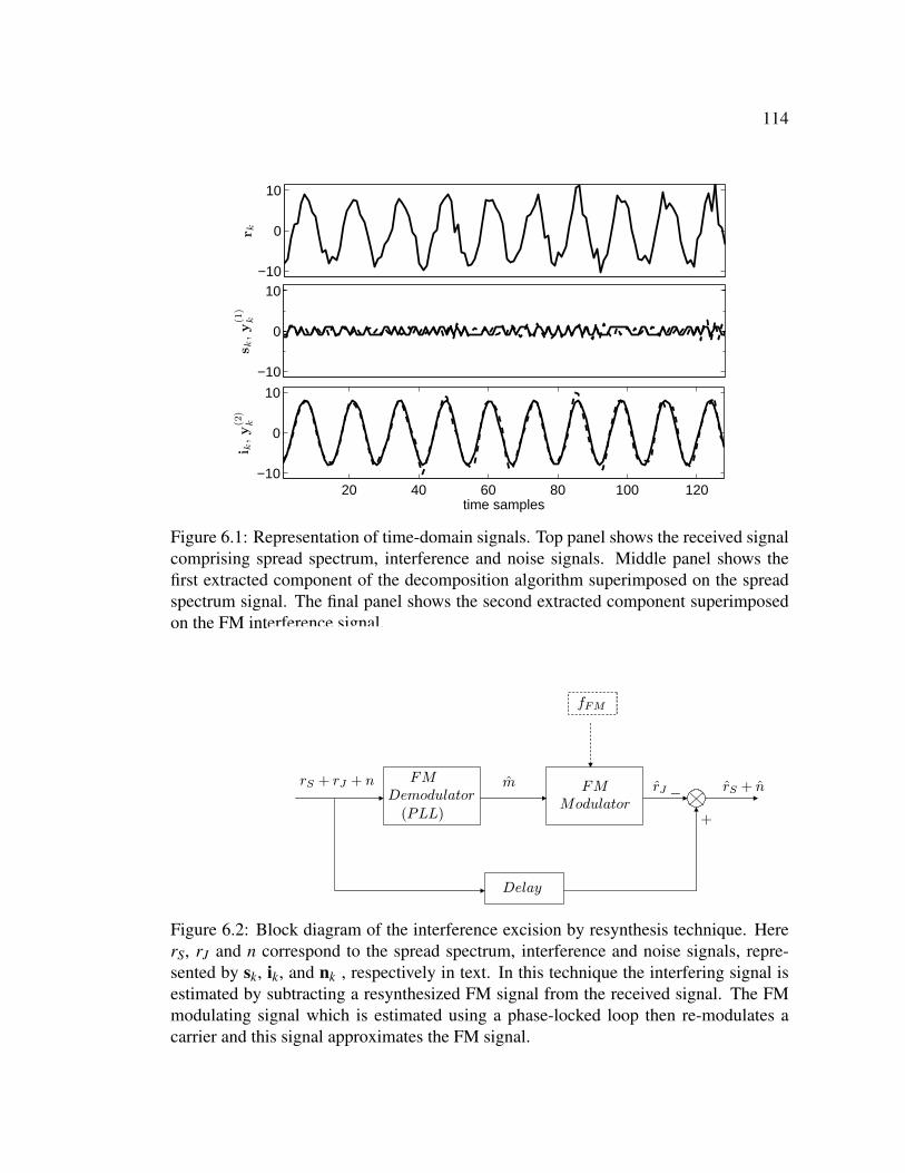
114
−10
0
10
rk
−10
0
10
sk,y
(1)
k
20 40 60 80 100 120−10
0
10
time samples
i k,y
(2)
k
Figure 6.1: Representation of time-domain signals. Top panel shows the received signalcomprising spread spectrum, interference and noise signals. Middle panel shows thefirst extracted component of the decomposition algorithm superimposed on the spreadspectrum signal. The final panel shows the second extracted component superimposedon the FM interference signal.
FMDemodulator(PLL)
FMModulator
m
+−
Delay
fFM
rS + rJ + n rJ rS + n
Figure 6.2: Block diagram of the interference excision by resynthesis technique. HererS, rJ and n correspond to the spread spectrum, interference and noise signals, repre-sented by sk, ik, and nk , respectively in text. In this technique the interfering signal isestimated by subtracting a resynthesized FM signal from the received signal. The FMmodulating signal which is estimated using a phase-locked loop then re-modulates acarrier and this signal approximates the FM signal.
115
resulting signal is processed and input into a threshold detector to estimate the transmit-
ted binary data sequence.
Let bk =±1 be the kth message symbol transmitted in a DSSS system such that
sk = bkck (6.1)
where ck = [ck(0), ...,ck(L−1)]T for k = 1,2, ... is a PN sequence with a chip length
L, cn =±1 is the nth chip of the PN sequence, and sk is the DSSS signal. The received
signal rk at the output of the BPSK demodulator will consist of the DSSS signal sk,
additive white Gaussian noise (AWGN) term nk, and interference term ik such that
rk = sk +nk + ik. (6.2)
At the receiver, to estimate bk, we use the PN sequence ck to despread rk, and integrate
the result to generate the test statistic Λk:
Λk = ⟨rk,ck⟩= cTk rk =
L−1
∑n=0
ck(n)rk(n). (6.3)
Using the test statistic Λk, we estimate the message symbols as
bk =
+1 , if Λk ≥ 0,
−1 , if Λk < 0. (6.4)
In the proposed technique the received signal rk is decomposed into two components
using the RCEMD algorithm, y(1)k and y(2)k . Analogous to wavelet decomposition, the
generated components have a decreasing trend of instantaneous frequencies. However,
unlike wavelets, the transition frequencies are not fixed; they are signal dependent. Since
the on-center interference has a smaller IF relative to the DSSS signal for a large time
fraction, it manifests itself in the second component, whereas the first generated compo-
nent closely resembles the spread spectrum signal. Therefore, the first component, y(1)k
is despread using the PN sequence to generate the test statistic Λk in a similar fashion
as represented in (6.3). The decomposition is stopped at the first level, after generation
of two components because the signal component corresponding to the spread spectrum
signal is generated first and the residue consists of interference and noise components
116
and is not useful in transmitted message symbol estimation. The result of the RCEMD
decomposition applied to the signal described in (6.2) is shown in Fig. 6.1. The first
panel shows the received signal, rk, the second shows the first decomposed component,
y(1)k , superimposed on the spread spectrum signal, ik, and the bottom panel shows the
interference signal (tone-modulated FM signal here) and the second component from
the RCEMD algorithm superimposed on each other. While the first RCEMD generated
component closely resembles the spread spectrum signal, sk, they are not identical due
to the presence of residual noise and in-band interference signal in the decomposition
result.
6.3 Simulation Results
The interference excision performance of the proposed RCEMD-based technique is
studied on the basis of achieved bit-error rate (BER) in this section. Two classes of
interferers are considered here: static partial band interferers comprising multiple tones,
and time-varying interferers modeled as FM signals. Further, we consider two kinds of
modulating signals for the FM signals: (a) simple tones , and (b) filtered noise follow-
ing an autoregressive (AR) model. These three classes of interferers are studied in this
section.
Some existing interference suppression techniques are also considered and their
BER performances are compared with our proposed technique in this section. Here
BER performance results for three alternate techniques are also presented. The first
method is a two-step procedure where the IF of the interfering signal is first estimated
using the Wigner-Ville distribution (WVD) and then a short, time-varying finite impulse
response (FIR) notch filter is designed to remove that signal [88]. The time-varying na-
ture of the FM interfering signal requires a short length notch filter, which corresponds
to a wide notch in the frequency domain, thereby also distorting the spread spectrum
signal. Secondly, we study the performance of a simple adaptive filter (AF) based on
the least-mean-square (LMS) algorithm at removing the primary signal at the secondary
receiver. A nine-tap adaptive FIR filter is considered for performance comparison in
all three cases. To allow convergence of filter coefficients, the initial data frames are
ignored while computing the BER for the adaptive filter technique.
The final method that we will study here involves subtracting a resynthesized FM
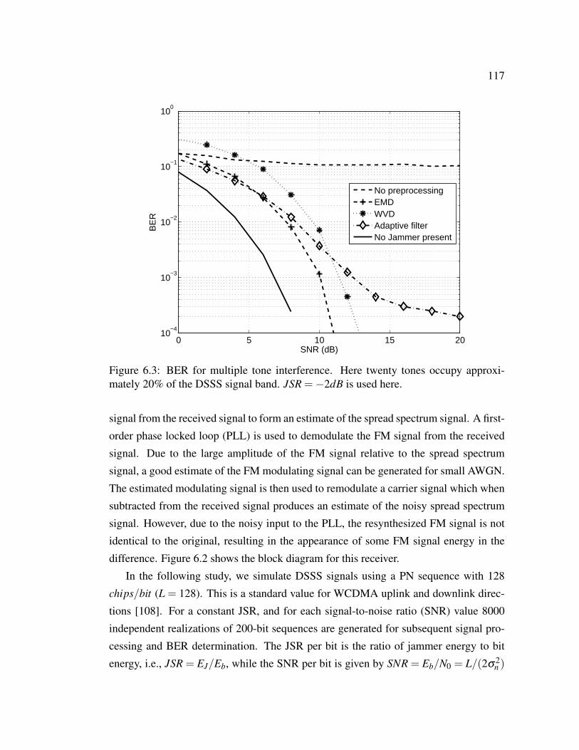
117
0 5 10 15 2010
−4
10−3
10−2
10−1
100
SNR (dB)
BE
R
No preprocessingEMDWVDAdaptive filterNo Jammer present
Figure 6.3: BER for multiple tone interference. Here twenty tones occupy approxi-mately 20% of the DSSS signal band. JSR =−2dB is used here.
signal from the received signal to form an estimate of the spread spectrum signal. A first-
order phase locked loop (PLL) is used to demodulate the FM signal from the received
signal. Due to the large amplitude of the FM signal relative to the spread spectrum
signal, a good estimate of the FM modulating signal can be generated for small AWGN.
The estimated modulating signal is then used to remodulate a carrier signal which when
subtracted from the received signal produces an estimate of the noisy spread spectrum
signal. However, due to the noisy input to the PLL, the resynthesized FM signal is not
identical to the original, resulting in the appearance of some FM signal energy in the
difference. Figure 6.2 shows the block diagram for this receiver.
In the following study, we simulate DSSS signals using a PN sequence with 128
chips/bit (L = 128). This is a standard value for WCDMA uplink and downlink direc-
tions [108]. For a constant JSR, and for each signal-to-noise ratio (SNR) value 8000
independent realizations of 200-bit sequences are generated for subsequent signal pro-
cessing and BER determination. The JSR per bit is the ratio of jammer energy to bit
energy, i.e., JSR = EJ/Eb, while the SNR per bit is given by SNR = Eb/N0 = L/(2σ2n )
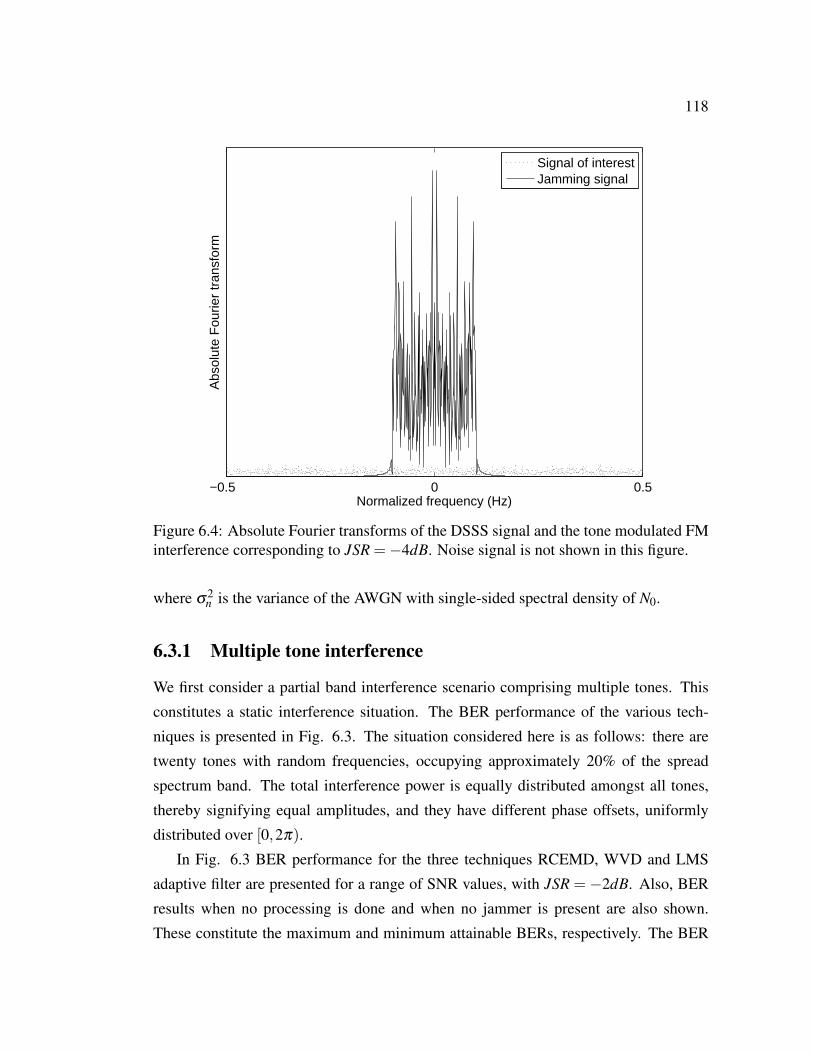
118
−0.5 0 0.5Normalized frequency (Hz)
Abs
olut
e F
ourie
r tr
ansf
orm
Signal of interestJamming signal
Figure 6.4: Absolute Fourier transforms of the DSSS signal and the tone modulated FMinterference corresponding to JSR =−4dB. Noise signal is not shown in this figure.
where σ2n is the variance of the AWGN with single-sided spectral density of N0.
6.3.1 Multiple tone interference
We first consider a partial band interference scenario comprising multiple tones. This
constitutes a static interference situation. The BER performance of the various tech-
niques is presented in Fig. 6.3. The situation considered here is as follows: there are
twenty tones with random frequencies, occupying approximately 20% of the spread
spectrum band. The total interference power is equally distributed amongst all tones,
thereby signifying equal amplitudes, and they have different phase offsets, uniformly
distributed over [0,2π).In Fig. 6.3 BER performance for the three techniques RCEMD, WVD and LMS
adaptive filter are presented for a range of SNR values, with JSR = −2dB. Also, BER
results when no processing is done and when no jammer is present are also shown.
These constitute the maximum and minimum attainable BERs, respectively. The BER

119
0
0.05
0.1
0.15
0.2
0.25
0.3
0.35
0.4
0.45
0.5
time
Nor
mal
ized
inst
anta
neou
s fr
eque
ncy
(Hz)
Figure 6.5: Instantaneous frequency of the tone-modulated FM signal.
of the proposed technique is found to be the smallest of the presented techniques and
there is an approximately 2dB gain over the WVD technique at BER = 10−4. A five-tap
filter was used to suppress the interference signal in the WVD technique. The adaptive
filter performance is observed to saturate for large SNR values because the filter noise is
essentially set by the interference level and frequencies and is unaffected by the additive
noise level at large SNRs.
6.3.2 Tone modulated FM interference
Here an FM interference signal is considered. The modulating signal is a sinusoid in
this case. The frequency domain representation of the interference and spread spectrum
signals is shown in Fig. 6.4 for JSR =−4dB. The IF of the interference signal for this
case is shown in Fig. 6.5. Again, approximately 20% of the spread spectrum band is
covered by FM interference. The BER performances of the different techniques when
JSR = −4dB are shown in Fig. 6.6. Here resynthesis technique performance is also
included. As before, the RCEMD technique produces smaller BER at large SNRs, with
the gain being approximately 2dB at BER = 10−4 over both WVD and adaptive filter

120
0 5 10 15 2010
−4
10−3
10−2
10−1
100
SNR (dB)
BE
R
No preprocessingEMDWVDResynthesisAdaptive filterNo Jammer present
Figure 6.6: BER for frequency modulated interference. Here simple tone modulation ofthe FM signal is considered. JSR =−4dB is used in this case.
techniques. The saturation of the resynthesis technique BER at large SNRs is because
its performance is essentially limited by the signal energy relative to jammer energy (via
JSR) and is unaffected by change in SNR for large values.
6.3.3 Filtered noise modulation of FM interferer
Finally, filtered noise modulation of the FM interference signal is considered. The
FM modulating signal in our experiments is generated using a general stochastic time-
varying model, namely a first-order auto-regressive (AR(1)) model. The choice of low-
order filter model is based on our experimental observation that the proposed technique
is insensitive to the model-order used for signal generation for the same signal band-
width. An approximately 20% spread spectrum band coverage by the FM interference
is simulated. The performance results are shown in Fig. 6.7. Here, the performance
advantage of the RCEMD technique over the next best, WVD, is approximately 1dB at
the reference BER level of 10−4. Here, results corresponding to JSR = 0dB are shown.

121
0 5 10 15 2010
−4
10−3
10−2
10−1
100
SNR (dB)
BE
R
No preprocessingEMDWVDResynthesisAdaptive filterNo Jammer present
Figure 6.7: BER for frequency modulated interference. Here the modulating signal isfiltered noise following an AR(1) model. JSR = 0dB is used here.
6.4 Conclusions
A novel technique for partial band interference excision using the RCEMD technique,
applicable to WCDMA communication system was presented in this chapter. Here
the received spread spectrum signal affected by interference and background noise is
decomposed into two components using the RCEMD technique. Due to the signal-
dependent decomposition property of the EMD-based technique, the two generated
components closely resemble the spread spectrum plus noise and the interference sig-
nals respectively. The extracted component corresponding to the spread spectrum signal
is despread using the spreading code to derive an estimate of the transmitted symbol.
The BER performance of this technique was compared to some alternate interference
excision techniques and improvement was observed. An advantage of an EMD-based
technique in interference excision is that no tuning of the technique based on a priori
knowledge of signal components is required unlike other techniques. Another advan-
tage of this technique that its performance is robust with respect to interference type,
whereas the performance of other techniques is observed to depend on the interference

122
type. However, the performance of this technique is seen to degrade when the interfer-
ence is off-center due to inability of the decomposition technique to produce high fidelity
representation of the spread spectrum and interference signals in separate components.
This aspect of the problem needs further investigation.
Part II
Signal Analysis of Sensor Data

Chapter 7
Atmospheric Pressure Signal Analysisusing Raised Cosine Empirical ModeDecomposition
The study of the atmospheric pressure is of interest to meteorologists in two ways: one
directly, and secondly via the study of gravity waves that can be inferred from the pres-
sure observations. A network of microbarographs is used by researchers to measure this
quantity. The presence of seasonally-varying diurnal and semidiurnal tides, cyclonic and
anticyclonic pressure variations, as well as sporadic events such as hurricanes often ob-
scures the quantities of interest to these researchers. It therefore becomes imperative for
the chosen data-processing method to effectively eliminate the effects of these features
before a meaningful analysis of the underlying phenomena can be performed. Naturally,
a technique based on the Fourier transform is inappropriate due to the poor time local-
ization of its basis functions. An EMD-based approach to eliminate these time-varying
quantities from microbarograph observations is presented here. Accurate estimation of
the diurnal and semidiurnal tide signals using EMD is demonstrated and its performance
compared to existing time-frequency techniques like wavelets and short-time Fourier
transform. The use of the EMD-based technique to isolate a hurricane signature is also
shown. Further, feature extraction using RCEMD algorithm is introduced in the final
section of the chapter and its advantages over the EMD technique are highlighted.

125
7.1 Introduction
Analysis of non-stationary and nonlinear processes poses serious challenges to tradi-
tional signal processing techniques. The transient nature of events in real-life situations
essentially limits the utility of the simple Fourier analysis, which has no time resolution.
The short time Fourier transform (STFT), or the spectrogram, allows time-frequency
analysis using the familiar fast Fourier transform (FFT). However, it has the disadvan-
tage of fixed time-frequency resolution and the implicit assumption of piecewise station-
arity of the signal, which is not valid in general. The wavelet transform method over-
comes some of the above limitations by allowing the decomposition of a signal into a
set of basis functions that are localized both in time and frequency. The need for a priori
knowledge about the kind of scale elements present in the signal and the corresponding
choice of wavelet to isolate them is a serious drawback of the wavelet transform method.
This has led to the widespread use of the EMD algorithm for analysis of nonstationary
signals.
A microbarograph operating at the Arecibo observatory (AO), Puerto Rico has been
taking almost continuous measurements of the tropical surface atmospheric pressure
since early 2003 (daily pressure plots updated at [109]). The microbarograph measures
pressure continuously with a sampling interval of 1 s and resolution of 10 µbar. An
interesting feature of atmospheric pressure data is the presence of tides of varying du-
rations. The 12-hour duration (semidiurnal) tides and the 24-hour duration (diurnal)
tides have their origins in the thermal heating of the atmosphere by the sun as well as
the gravitational attraction of the sun and the moon. Further, the elliptical orbit of the
earth around the sun results in seasonal variations in the amplitude of these tides. A
thorough explanation of the physics behind atmospheric tides can be found in [110].
The semidiurnal tide, being the strongest, is plainly visible in a plot of the time-series
signal from the microbarograph. However, superimposed variations of longer periods
and other transient pressure changes make accurate measurement of the semidiurnal and
diurnal tide amplitudes difficult to obtain. In this chapter we present a new EMD-based
technique to extract the diurnal and semidiurnal tides from the pressure data. Results are
presented for normal conditions as well as for an instance of severe pressure disturbance
due to a passing hurricane. We also present results obtained from applying the wavelet
transform technique to the same data for comparison. Finally, signal feature extraction
126
using RCEMD is introduced and its advantages highlighted.
7.2 Data analysis using HHT and wavelets
We briefly describe here the important steps involved in the HHT technique (details can
be found in Chapter 2). First step is to find the IMFs by a procedure termed “sifting” or
empirical mode decomposition (EMD) in [27]. This involves projecting the signal onto
basis functions that are implicitly defined and signal-dependent. Unlike traditional sig-
nal decomposition techniques such as wavelets and STFT that decompose the original
signal into a series of constituents of fixed, pre-determined frequencies, the generated
IMFs do not necessarily have constant frequency or amplitude and it is for this reason
that it is often difficult to assign any physical meaning to them. Next step in this pro-
cess involves computing the instantaneous frequency of each IMF by first evaluating its
Hilbert transform, followed by evaluating the derivative of the phase. Mathematically,
the Hilbert transform of a real-valued function x(t) is defined as (see [111])
x(t) =∫ ∞
−∞
x(u)π(t −u)
du, (7.1)
θ(t) = arctan[
x(t)x(t)
], (7.2)
and
f0(t) =(
12π
)dθ(t)
dt(7.3)
is the instantaneous frequency. The instantaneous frequency of each IMF is superim-
posed and presented as a color coded map, with optional smoothing applied. This is
referred to as the Hilbert spectrum of the signal and is analogous to the wavelet spec-
trum. We next present the equations defining the continuous wavelet transform (CWT)
and its inverse (see [112]):
Xw(b,a) =1|a|
∫ ∞
−∞x(t)ψ∗
(t −b
a
)(7.4)
and

127
x(t) =Cψ−1∫ ∞
−∞
∫ ∞
−∞Xw(b,a)ψb,a(t)
dadb|a|
(7.5)
where
Cψ =∫ ∞
−∞
|ψ(ω)|2
|ω |dω < ∞ (7.6)
and
ψb,a(t) =1|a|
ψ(
t −ba
)(7.7)
where ψ(ω) is the Fourier transform of the mother wavelet ψ(t).
In this work we have utilized the code available at [83] to implement the HHT tech-
nique. A few pre-processing steps were carried out on the raw data before applying the
time-frequency techniques. First, since we are interested in events with periods longer
than 6 hours, we time averaged the data to get sampling interval of 3 hours. Some gaps
were observed in the existing data due to equipment malfunction. Over the two-year
period for which data is available loss of data spanning a period of about half a day
was observed twelve times and on one occasion we do not have data for a two day pe-
riod. These gaps in data were interpolated using sine waves. Finally, it was observed
that the non-zero mean of the data causes considerable ringing to appear at the win-
dow edges in results using traditional techniques like wavelets and short time Fourier
transform (STFT), whereas EMD remains unaffected by the non-zero mean of the data.
Hence, mean removal was carried out prior to analysis by each of the techniques to get
meaningful results in all cases. Figure 7.1 shows the time series, IMFs and the Hilbert
spectrum computed for the pressure data for a two year period starting at 00:00 AST 1
January, 2004. Severe pressure fluctuations due to a passing hurricane event are visible
during days 258-259 in the time series, Hilbert spectrum and some of the IMFs. The
semidiurnal and diurnal tides are also visible in the Hilbert spectrum. Results from some
competing techniques are presented in Fig. 7.2 for the same record. In the wavelet spec-
trum presented in Fig. 7.2a, although the hurricane event is clearly defined, considerable
smearing is evident in 24-hour tide while the 12-hour tide is practically undetectable.
The mother wavelet used to analyze the signal was the analytic signal whose real part is
the fourth derivative of the Gaussian with variance equal to one (see [112]). The real,

128
100 200 300 400 500 600 700962
964
966
968
970
972
974
976
978
980
Time (days)
Pres
sure
(m
bar)
Hurricane
(a)
−505
−505
−505
−505
−505
−202
Pre
ssur
e (m
bar)
−202
−505
−505
−101
0 100 200 300 400 500 600 7000
0.51
Time (days)
(b)
Figure 7.1

129
Time (days)
Fre
quen
cy (
Hz)
100 200 300 400 500 600 700
0.5
1
1.5
2
2.5
3
3.5
4
4.5
x 10−5
12−hour tide
24−hour tideHurricane
(c)
Figure 7.1: Microbarograph data 1 January 2004 - 31 December 2005: (a) time series,(b) IMFs computed using EMD, (c) Hilbert spectrum with 12-hour, 24-hour tides andhurricane events visible.
imaginary and absolute values of the basic wavelet are shown in Fig. 7.3. Good time
localization property of this mother wavelet assures efficient filtering of solitary waves
or bumps that are intrinsically very localized in time. The second existing technique that
we evaluated is the STFT. Results for the STFT technique using the Hamming window
are shown in Fig. 7.2b. Signatures of the two tides and the hurricane are visible in the
spectrum. The presence of a transient event as well as underlying periodic events in
the data requires careful selection of window length. A window length of 60 samples,
corresponding to 7.5 days offers a good compromise between requirements of high time
resolution and high frequency resolution for optimum representation of the hurricane
event and the persistent tides respectively. It must be noted here that the HHT procedure
does not require similar signal-dependent tuning of parameters to optimize the decom-
position quality. Finally, tides of different durations show up quite clearly in the FFT
plot, which is expected because Fourier analysis is known to be an efficient representa-
130
tion of stationary signals.
7.3 Signal Feature Extraction
Next we proceed with signal feature extraction using EMD. As mentioned earlier, the
IMFs that are produced using the EMD procedure do not necessarily have constant fre-
quency. In fact, when applied to real-life signals where irregular structure is common,
the sifting process distributes signal components of a particular frequency among sev-
eral IMFs. Figure 7.4 shows several instances of overlap of instantaneous frequencies
of adjacent IMFs. This leads us to the conclusion that to extract a particular frequency
component from a signal, it is not sufficient to select the IMF that produces that partic-
ular instantaneous frequency. Rather, a few neighboring IMFs that have instantaneous
frequencies equal to the desired frequency at certain instants need to be included too.
Further, in order to take into account the effect of noise and other irregularities in the
signal, instead of a single frequency we consider a small band of frequencies centered
on the desired frequency to decide which IMFs to combine to get the desired frequency
component.
We describe a practical way of implementing the signal extraction process here. The
initial steps, viz., sifting, forming analytic signals, and finding instantaneous frequency
are performed as usual. Next we form a small band of frequencies around the desired
frequency according to the tolerance level desired. In this particular case placing the
frequency band limits at 90% and 110% of the desired frequency appears to include
most of the energy of the relevant IMF as indicated by the two horizontal lines in Fig.
7.5. In other practical cases the frequency band will need adjusting so that most of the
energy of the desired IMF is contained within it. However, expanding the frequency
band excessively will result in inclusion of spurious energy from adjacent IMFs leading
to contamination of the extracted feature by other undesired features. Further research
is required to develop a realizable mapping between features in the time domain and
their corresponding projections in the IMF domain leading to an automatic selection of
IMF sections. Next we form an “inclusion matrix” to decide which IMFs are combined
together at each instant to form the signal of desired frequency. The number of rows of
the inclusion matrix equals the number of computed IMFs and the column count equals
the number of time samples in the signal. The matrix is initially set to all zeroes. Then

131
Time (days)
Fre
quen
cy (
Hz)
100 200 300 400 500 600 700
0.5
1
1.5
2
2.5
3
3.5
4
4.5
x 10−5
Hurricane
24−hour tide
(a)
Time (days)
Fre
quen
cy (
Hz)
100 200 300 400 500 600 7000
0.5
1
1.5
2
2.5
3
3.5
4
4.5
x 10−5
12−hour tide
24−hour tide
Hurricane
(b)
Figure 7.2

132
0 0.5 1 1.5 2 2.5 3 3.5 4 4.5 5
x 10−5
0
0.1
0.2
0.3
0.4
0.5
0.6
0.7
0.8
0.9
1
Frequency (Hz)
Nor
mal
ized
abs
olut
e va
lue
6−hour tide
24−hour tide
12−hour tide
8−hour tide
(c)
Figure 7.2: Microbarograph data 1 January 2004 - 31 December 2005: (a) wavelet spec-trum using complex mother wavelet, (b) short time Fourier transform spectrum usingHamming window, (c) fast Fourier transform with frequency bins corresponding to 24,12, 8, 6-hour tides showing large amplitudes.
at each time instant a ‘1’ is placed at the position corresponding to an IMF that has
its instantaneous frequency within the frequency band set earlier. When this procedure
is completed for the entire time duration, the matrix containing the IMFs as its rows
is multiplied by the inclusion matrix and the components added up to get the desired
frequency signal component. The concept of overlap of instantaneous frequencies of
IMFs and the desired frequency thresholds is shown in Fig. 7.5 for extracting the 24-
hour tide from the microbarograph observations. The results of this technique are shown
in Fig. 7.6 where we present the 12 and 24-hour tides extracted from the microbarograph
observations using the above procedure. Clear seasonal variations are observed in the
extracted 12-hour tide signal.
We now demonstrate a sporadic feature signature isolation technique using EMD.
Effects of a passing hurricane were observed in the microbarograph data from 14-15
September 2004. The presence of such a large energy event in the observations some-
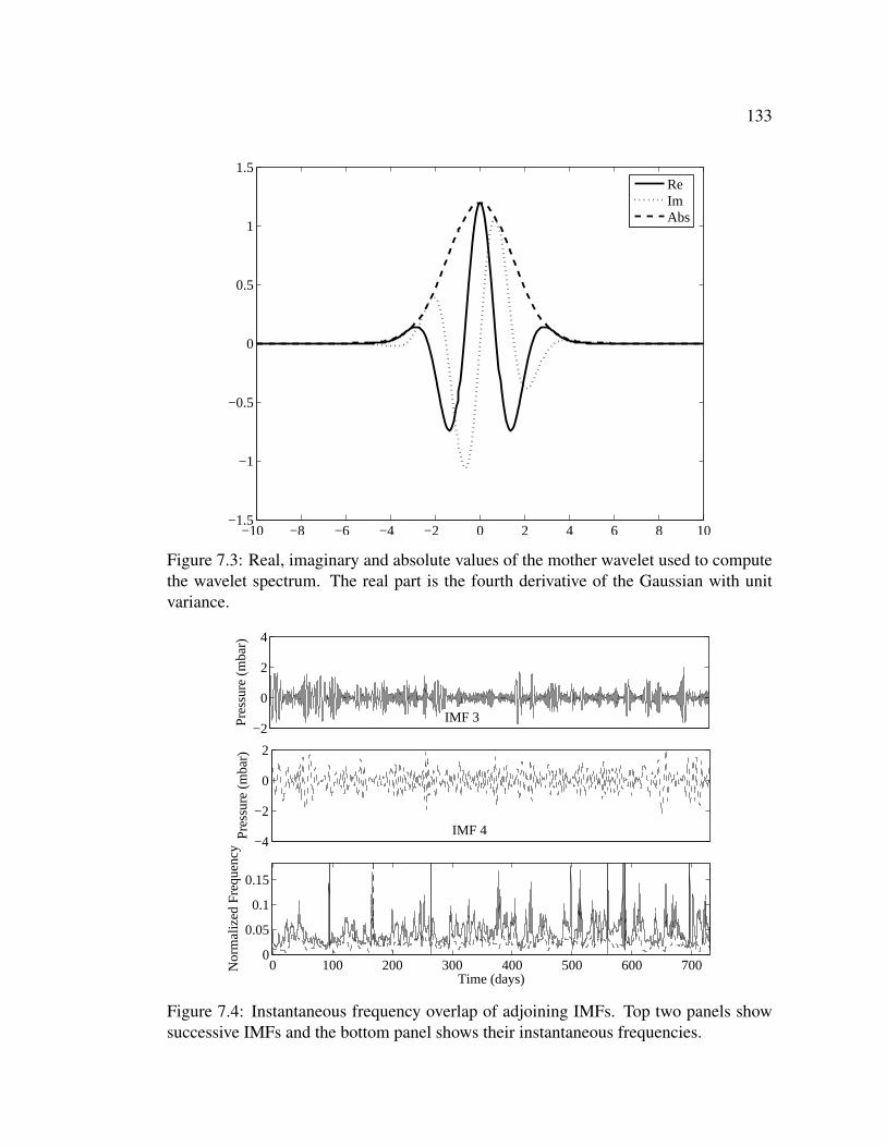
133
−10 −8 −6 −4 −2 0 2 4 6 8 10−1.5
−1
−0.5
0
0.5
1
1.5ReImAbs
Figure 7.3: Real, imaginary and absolute values of the mother wavelet used to computethe wavelet spectrum. The real part is the fourth derivative of the Gaussian with unitvariance.
−2
0
2
4
Pre
ssur
e (m
bar)
−4
−2
0
2
Pre
ssur
e (m
bar)
0 100 200 300 400 500 600 7000
0.05
0.1
0.15
Nor
mal
ized
Fre
quen
cy
Time (days)
IMF 3
IMF 4
Figure 7.4: Instantaneous frequency overlap of adjoining IMFs. Top two panels showsuccessive IMFs and the bottom panel shows their instantaneous frequencies.
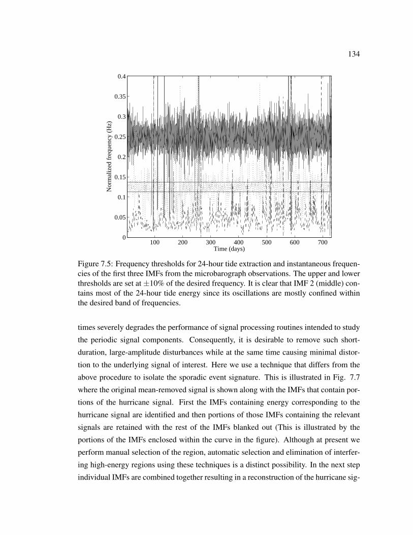
134
100 200 300 400 500 600 7000
0.05
0.1
0.15
0.2
0.25
0.3
0.35
0.4
Time (days)
Nor
mal
ized
fre
quen
cy (
Hz)
Figure 7.5: Frequency thresholds for 24-hour tide extraction and instantaneous frequen-cies of the first three IMFs from the microbarograph observations. The upper and lowerthresholds are set at ±10% of the desired frequency. It is clear that IMF 2 (middle) con-tains most of the 24-hour tide energy since its oscillations are mostly confined withinthe desired band of frequencies.
times severely degrades the performance of signal processing routines intended to study
the periodic signal components. Consequently, it is desirable to remove such short-
duration, large-amplitude disturbances while at the same time causing minimal distor-
tion to the underlying signal of interest. Here we use a technique that differs from the
above procedure to isolate the sporadic event signature. This is illustrated in Fig. 7.7
where the original mean-removed signal is shown along with the IMFs that contain por-
tions of the hurricane signal. First the IMFs containing energy corresponding to the
hurricane signal are identified and then portions of those IMFs containing the relevant
signals are retained with the rest of the IMFs blanked out (This is illustrated by the
portions of the IMFs enclosed within the curve in the figure). Although at present we
perform manual selection of the region, automatic selection and elimination of interfer-
ing high-energy regions using these techniques is a distinct possibility. In the next step
individual IMFs are combined together resulting in a reconstruction of the hurricane sig-

135
965
970
975
980
−2
0
2 12−hour tide
Pre
ssur
e (m
bar)
0 100 200 300 400 500 600 700
−2
0
2 24−hour tide
Time (Days)
Figure 7.6: 12-hour (semidiurnal) and 24-hour (diurnal) tides extracted from the originalmicrobarograph observations (on top) using the EMD-based technique described in text.
nal, which can then be subtracted from the original signal. Results of alternate feature
extraction using this method are shown in Fig. 7.8a. For comparison we also present
results using an analogous technique based on wavelets (see [112]) in Fig. 7.8b. Both
figures show the original signal, the extracted signal feature and the residue.
Some observations regarding these results are in order. First, the start and end of
the extracted event is rather abrupt using the EMD-based technique while it is more
gradual for the wavelet based one. This is a direct consequence of how the IMFs are
combined in the “inverse EMD” process (where an IMF component is either included
or not included in the reconstruction process) and the way the inverse CWT operation
works (which is more like a convolution operation over the desired region). Secondly,
from observing the residues using the two techniques it is clear that the effect of the
EMD-based technique is to remove all frequency components from the affected period
whereas the wavelet method attempts to maintain continuity as far as the low energy
background signal is considered. Which of the two approaches is desirable depends
upon the particular application since although removal of all frequency components in
the EMD case may be unacceptable in some situations, the tendency of the wavelet ap-
proach to maintain continuity in the low energy signal may introduce severe distortions
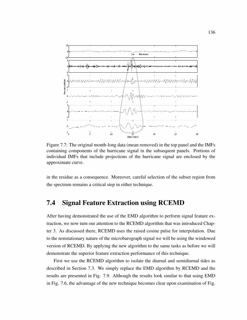
136
Figure 7.7: The original month-long data (mean removed) in the top panel and the IMFscontaining components of the hurricane signal in the subsequent panels. Portions ofindividual IMFs that include projections of the hurricane signal are enclosed by theapproximate curve.
in the residue as a consequence. Moreover, careful selection of the subset region from
the spectrum remains a critical step in either technique.
7.4 Signal Feature Extraction using RCEMD
After having demonstrated the use of the EMD algorithm to perform signal feature ex-
traction, we now turn our attention to the RCEMD algorithm that was introduced Chap-
ter 3. As discussed there, RCEMD uses the raised cosine pulse for interpolation. Due
to the nonstationary nature of the microbarograph signal we will be using the windowed
version of RCEMD. By applying the new algorithm to the same tasks as before we will
demonstrate the superior feature extraction performance of this technique.
First we use the RCEMD algorithm to isolate the diurnal and semidiurnal tides as
described in Section 7.3. We simply replace the EMD algorithm by RCEMD and the
results are presented in Fig. 7.9. Although the results look similar to that using EMD
in Fig. 7.6, the advantage of the new technique becomes clear upon examination of Fig.

137
950
960
970
980
−20
−10
0
10
Pre
ssur
e (m
bar)
0 5 10 15 20 25 30965
970
975
980
Time (Days)
(a)
950
960
970
980
−20
−10
0
10
Pre
ssur
e (m
bar)
0 5 10 15 20 25 30965
970
975
980
Time (Days)
(b)
Figure 7.8: Results for alternate event extraction for (a) EMD-based technique; and (b)wavelet based technique, for a hurricane event observed in the microbarograph data inSeptember 2004. The three panels show the original month-long data, the extractedhurricane event and the residue after event removal from top to bottom respectively.
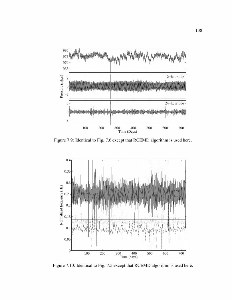
138
965
970
975
980
−2
0
2 12−hour tide
Pre
ssur
e (m
bar)
100 200 300 400 500 600 700
−2
0
2 24−hour tide
Time (Days)
Figure 7.9: Identical to Fig. 7.6 except that RCEMD algorithm is used here.
100 200 300 400 500 600 7000
0.05
0.1
0.15
0.2
0.25
0.3
0.35
0.4
Time (days)
Nor
mal
ized
fre
quen
cy (
Hz)
Figure 7.10: Identical to Fig. 7.5 except that RCEMD algorithm is used here.
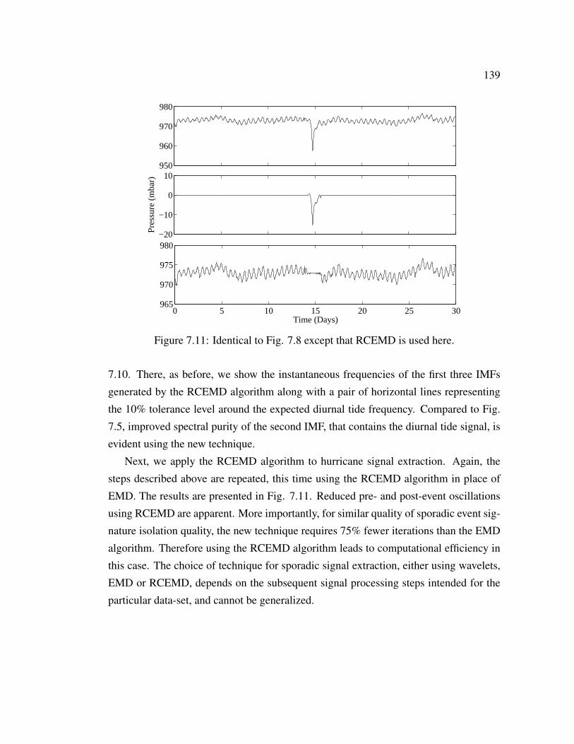
139
950
960
970
980
−20
−10
0
10
Pre
ssur
e (m
bar)
0 5 10 15 20 25 30965
970
975
980
Time (Days)
Figure 7.11: Identical to Fig. 7.8 except that RCEMD is used here.
7.10. There, as before, we show the instantaneous frequencies of the first three IMFs
generated by the RCEMD algorithm along with a pair of horizontal lines representing
the 10% tolerance level around the expected diurnal tide frequency. Compared to Fig.
7.5, improved spectral purity of the second IMF, that contains the diurnal tide signal, is
evident using the new technique.
Next, we apply the RCEMD algorithm to hurricane signal extraction. Again, the
steps described above are repeated, this time using the RCEMD algorithm in place of
EMD. The results are presented in Fig. 7.11. Reduced pre- and post-event oscillations
using RCEMD are apparent. More importantly, for similar quality of sporadic event sig-
nature isolation quality, the new technique requires 75% fewer iterations than the EMD
algorithm. Therefore using the RCEMD algorithm leads to computational efficiency in
this case. The choice of technique for sporadic signal extraction, either using wavelets,
EMD or RCEMD, depends on the subsequent signal processing steps intended for the
particular data-set, and cannot be generalized.

140
7.5 Conclusion
In this chapter we have studied the EMD technique for signal event extraction, utiliz-
ing microbarograph observations from Arecibo Observatory. We compared the Hilbert
spectrum derived using the HHT technique with the wavelet spectrum using a complex
wavelet and demonstrated considerable improvement in clarity in the representation of
tides by the Hilbert spectrum over the wavelet spectrum. Next we demonstrated a tech-
nique for signal feature extraction based on the EMD. Application of this signal feature
extraction technique to extract diurnal and semidiurnal tides from the atmospheric pres-
sure data was presented. High precision in the extracted signal allows observation of
the seasonal variations in the semidiurnal tides quite clearly. Further, we adapted the
signal feature extraction technique to isolate and remove large amplitude disturbances
from time-series data. Performance of this technique is demonstrated via extraction of
a hurricane event from the pressure observations. Further improvement in performance
is demonstrated by the use of RCEMD. Performance of the newly developed feature
extraction techniques is compared to that of a wavelet based technique using a complex
wavelet. Relative advantages of each technique are highlighted and situations where
either approach might find favor are pointed out.

Chapter 8
Genetic Algorithm based ParameterEstimation Technique for FragmentingRadar Meteor Head-echoes
Meteoroid fragmentation presents a serious problem for Doppler estimation using Fourier
transform techniques. Radar returns from multiple, closely-spaced bodies traveling at
nearly identical speeds result in an interference pattern which makes it difficult to esti-
mate properties of individual bodies by traditional techniques. Here we present a genetic
algorithm based procedure to determine the properties of the individual fragments, such
as relative scattering cross-section, speed and deceleration. The radar meteor observa-
tions presented here were made using the Poker Flat (Alaska) Incoherent Scatter Radar
(PFISR) operating at 449.3 MHz.
8.1 Introduction
The scientific community has been interested in observing sporadic radar meteors due
to the role of meteoroids in understanding space weather, in the aeronomy of the meteor
zone and in various aspects of plasma physics [113, 114]. Here we consider “head-
echo” observations in which radar returns are from the distribution of plasma imme-
diately surrounding the meteoroid and that travels with the meteoroid itself. For de-
tails regarding scattering mechanism and models of head-echoes the reader is referred
to [113, 115–117]. For meteor events observed in more than four radar pulses, a fast

142
Figure 8.1: Range-Time-Intensity (RTI) and Signal-to-Noise Ratio (SNR-similar to op-tical meteor light curves) of three meteor events observed with the Poker Flat 449.3 MHzIncoherent Scatter Radar (PFISR). The (a.) event (Event 1) is consistent with two mete-oroids traveling along the same trajectory and each producing a headecho that result inthe strong “interference” pattern. The (b.) event (Event 2) shows a more complex struc-ture that is consistent with three meteoroid fragments. The (c.) event (Event 3) whichshows strong frequency modulation of the SNR curve is otherwise similar to event 1.
Fourier transform (FFT) based technique has been developed that provides estimates of
the event altitude, signal-to-noise ratio (SNR) and speed as a function of time through-
out the event [118–121]. Many events having high enough SNR also yield deceleration
estimates.
Fragmented meteoroids present a problem for speed estimation using FFT tech-
niques. Scattering from two nearby slowly separating “point” targets (relative to the
wavelength) exhibit strong interference effects as the two signals add in-phase and out
of phase. That is, two (or more) common-trajectory meteoroid fragments exist within the
radar range resolution “cell” and, as the scattered electric fields exhibit nearly common
Doppler phase effects, the net electric field at the receiver shows a strong interference
pattern. Some researchers have previously tried to estimate the properties of fragmented
meteoroids in the past [122,123]. Further, the authors of [124] reported evidence of frag-
mentation based on their observations but stopped short of analyzing them. We present
here a genetic algorithm (GA) [125, 126] based optimization technique that searches
the multidimensional fragment parameter space to find the parameter set that minimizes
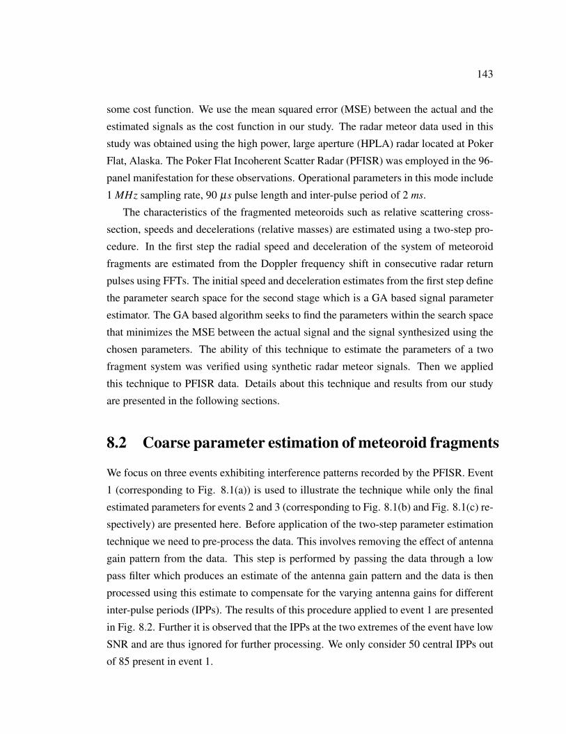
143
some cost function. We use the mean squared error (MSE) between the actual and the
estimated signals as the cost function in our study. The radar meteor data used in this
study was obtained using the high power, large aperture (HPLA) radar located at Poker
Flat, Alaska. The Poker Flat Incoherent Scatter Radar (PFISR) was employed in the 96-
panel manifestation for these observations. Operational parameters in this mode include
1 MHz sampling rate, 90 µs pulse length and inter-pulse period of 2 ms.
The characteristics of the fragmented meteoroids such as relative scattering cross-
section, speeds and decelerations (relative masses) are estimated using a two-step pro-
cedure. In the first step the radial speed and deceleration of the system of meteoroid
fragments are estimated from the Doppler frequency shift in consecutive radar return
pulses using FFTs. The initial speed and deceleration estimates from the first step define
the parameter search space for the second stage which is a GA based signal parameter
estimator. The GA based algorithm seeks to find the parameters within the search space
that minimizes the MSE between the actual signal and the signal synthesized using the
chosen parameters. The ability of this technique to estimate the parameters of a two
fragment system was verified using synthetic radar meteor signals. Then we applied
this technique to PFISR data. Details about this technique and results from our study
are presented in the following sections.
8.2 Coarse parameter estimation of meteoroid fragments
We focus on three events exhibiting interference patterns recorded by the PFISR. Event
1 (corresponding to Fig. 8.1(a)) is used to illustrate the technique while only the final
estimated parameters for events 2 and 3 (corresponding to Fig. 8.1(b) and Fig. 8.1(c) re-
spectively) are presented here. Before application of the two-step parameter estimation
technique we need to pre-process the data. This involves removing the effect of antenna
gain pattern from the data. This step is performed by passing the data through a low
pass filter which produces an estimate of the antenna gain pattern and the data is then
processed using this estimate to compensate for the varying antenna gains for different
inter-pulse periods (IPPs). The results of this procedure applied to event 1 are presented
in Fig. 8.2. Further it is observed that the IPPs at the two extremes of the event have low
SNR and are thus ignored for further processing. We only consider 50 central IPPs out
of 85 present in event 1.

144
Next we form an initial estimate of the Doppler speed and deceleration of the me-
teoroid fragments by examining the FFT of the data. The Doppler speed is determined
using the method described in [119]: the FFT is evaluated for each radar pulse and the
location of the peak absolute value gives the dominant frequency component present in
the pulse. It is found that the individual Doppler estimates vary substantially for each
IPP. This variation is due in part to the large variations in SNR due to fading. How-
ever, even in most of the deep “nulls” the SNR remains substantial. Another source of
Doppler error is that the phase evolution during each pulse is somewhat ambiguous due
to the presence of two similar Doppler signatures. A general decrease in the estimated
speed as time progresses is also observed that indicates deceleration. The deceleration
can be estimated from the slope of the linear fit to the speed vs. IPP (or time) values. It
must be emphasized here that the speed estimates that we obtain are the radial or line-
of-sight (LOS) values - deriving the velocity vector usually requires an interferometric
and/or multistatic radar system, which we did not use for these observations. For event
1 the radial (line-of-sight) entry speed of the system of fragments and the deceleration
estimated from the linear fit are 12.5 km/s and 12.1 km/s2 respectively.
8.3 Fine parameter estimation for individual fragments
using GA
The GA based technique is designed to provide us with estimates of the parameters
(amplitude, speed and deceleration) of each fragment in the system. The GA algorithm
starts with an initial population of random candidate parameters that are uniformly dis-
tributed over a small range around the initial Doppler estimates obtained from stage 1
of the technique. We define this range to be 0.5 km/s on either side of the radial speed
estimate and 4 km/s2 for deceleration estimate from stage 1. Then through a process of
selection (that refers to a process of choosing a proportion of the population based on
“fitness”), crossover (or recombination, that refers to reproduction) and mutation (that
refers to random changes in attributes of the offsprings to maintain diversity in popu-
lation) successive generations possess “better characteristics”, which in our case refers
to lower MSE. After some pre-determined number of generations or when the average
MSE of the population at a particular generation reaches a pre-defined minimum we

145
20 40 60 80 100 120 140 160
200400600800
Absolute value (averaged over all range cells)
20 40 60 80 100 120 140 160
200
400
600Antenna gain pattern estimate: LPF
20 40 60 80 100 120 140 160
−0.5
0
0.5
Compensated data
t (ms)
Figure 8.2: Event 1 power signal at various stages of the pre-processing step to estimateand remove antenna pattern.
stop the iterations and select from the final population the individual solution with the
best characteristics as the final estimate.
Before moving on to GA based parameter estimation, a brief description of the
physics of radar scattering from a point target is presented here. Consider that the ith
meteoroid fragment is at range Ri(t0) at reference time t0. Then the complex baseband
signal for the fragment is given by
xi(t) = Ai exp(
i4πRi(t)λ
t)
(8.1)
where Ri(t), the range of the ith fragment at time t is given by
Ri(t) = Ri(t0)− (vi −dit2)t. (8.2)
Here vi is the speed at time t0, di is the deceleration, Ai is amplitude of the ith fragment
and λ is the radar wavelength. The resultant signal, the baseband voltage, is the sum
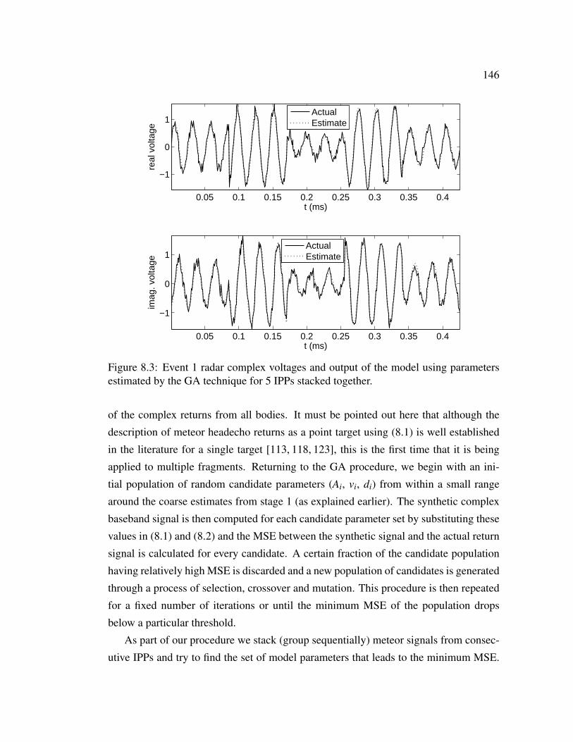
146
0.05 0.1 0.15 0.2 0.25 0.3 0.35 0.4
−1
0
1
t (ms)
real
vol
tage
0.05 0.1 0.15 0.2 0.25 0.3 0.35 0.4
−1
0
1
t (ms)
imag
. vol
tage
ActualEstimate
ActualEstimate
Figure 8.3: Event 1 radar complex voltages and output of the model using parametersestimated by the GA technique for 5 IPPs stacked together.
of the complex returns from all bodies. It must be pointed out here that although the
description of meteor headecho returns as a point target using (8.1) is well established
in the literature for a single target [113, 118, 123], this is the first time that it is being
applied to multiple fragments. Returning to the GA procedure, we begin with an ini-
tial population of random candidate parameters (Ai, vi, di) from within a small range
around the coarse estimates from stage 1 (as explained earlier). The synthetic complex
baseband signal is then computed for each candidate parameter set by substituting these
values in (8.1) and (8.2) and the MSE between the synthetic signal and the actual return
signal is calculated for every candidate. A certain fraction of the candidate population
having relatively high MSE is discarded and a new population of candidates is generated
through a process of selection, crossover and mutation. This procedure is then repeated
for a fixed number of iterations or until the minimum MSE of the population drops
below a particular threshold.
As part of our procedure we stack (group sequentially) meteor signals from consec-
utive IPPs and try to find the set of model parameters that leads to the minimum MSE.

147
0 20 40 60 80 100 120 140
0.1
0.2
0.3
0.4
0.5
0.6
f (kHz)
abs.
val
ue
ActualEstimate
Figure 8.4: Fast Fourier transform of actual signal and output of the model using param-eters estimated by the GA technique for event 1.
The issue of how many IPPs to stack together for GA analysis needs some discussion.
On the one hand a longer time series leads to better estimate of model parameters espe-
cially if the number of parameters to be estimated is large, while on the other hand, the
fact that the parameters of the meteoroid fragments change continuously as they travel
through the atmosphere would indicate that considering a smaller data series would bet-
ter capture the transient parameters of the bodies by our simple model. Analysis of
five fragmentation events from the database indicates that NIPP = 5 optimizes fragment
parameter estimation.
The next task is to determine the model order. Since the number of scattering frag-
ments is not known in advance, we assume one meteoroid fragment to be present ini-
tially and then progressively increase the number of fragments assumed in the model to
determine the model size at which the MSE value stops decreasing. For event 1 we de-
termined that two fragments are present and the individual parameters are listed in Table
8.1. Only the first 35 IPPs yielded reliable estimates of the parameters and are included
in the table. The closeness of the model generated using the estimated parameters and
148
rang
e (k
m)
Actual radar signal (after pre−processing)
85
90
95
0.5
1
1.5
t (ms)
rang
e (k
m)
Reconstructed signal using estimated parameters
0 10 20 30 40 50 60
85
90
95
0.5
1
1.5
Figure 8.5: Range-time-intensity (RTI) plot of the actual radar signal after pre-processing (upper panel), and reconstructed RTI plot using estimated parameters fromour technique (lower panel) for event 1.
the actual radar signal is shown in Fig. 8.3 and Fig. 8.4 where we show the time series
and the absolute value of the FFT of the actual radar signal and the estimated model.
Also by examining the initial speeds and the decelerations we can project back in time
to determine when the speeds of the two fragments are equal which would indicate the
time when fragmentation occurred. For event 1 we determined that fragmentation oc-
curred 460 ms before the fragments entered the radar beam, assuming their parameters
remained constant.
Further, using the estimated values of radial speed and deceleration we can calculate
how rapidly the two fragments are separating from each other. The estimated parame-
ters indicate that the separation between the fragments increases by about 6 m over the
duration of 70 ms for which parameter estimates are available. Finally, in Fig. 8.5 we
show the reconstructed range-time-intensity (RTI) plot for the portion of the event for
which we estimate the parameters. This seems to match the RTI plot of the actual radar
signal, which of course also includes background noise.

149
Table 8.1: Modeled parameters of meteor event 1.
IPP Relative amplitude Initial speed (km/s) Deceleration (km/s2)Body 1 Body 2 Body 1 Body 2 Body 1 Body 2
1-5 1 0.5937 12.628 12.532 10.555 10.7636-10 1 0.5937 12.519 12.428 10.062 10.445
11-15 1 0.5937 12.413 12.324 10.135 10.50016-20 1 0.6493 12.304 12.219 9.5538 11.56621-25 1 0.6996 12.192 12.103 8.9227 9.033326-30 1 0.7191 12.093 12.010 11.051 12.17731-35 1 0.7707 11.812 11.734 9.7296 12.000
Table 8.2: Modeled parameters of meteor event 2.
IPP Relative amplitude Initial speed (km/s) Deceleration (km/s2)Body 1 Body 2 Body 3 Body 1 Body 2 Body 3 Body 1 Body 2 Body 3
1-5 1 0.8453 0.6050 21.704 21.759 21.450 51.650 50.433 42.7106-10 1 0.8163 0.4283 21.469 21.555 21.023 40.681 47.089 32.226
11-15 1 0.7224 0.2986 20.875 21.216 20.768 47.283 56.154 47.54616-20 1 0.9021 0.5092 20.816 20.997 20.311 75.442 52.605 36.21521-25 1 0.8890 0.5088 20.026 20.372 19.864 26.036 15.618 37.03326-30 1 0.8922 0.5107 19.589 20.022 19.311 68.718 43.410 50.551
Event 2 appears to have a more complicated structure compared to event 1. A close
examination of the RTI plot reveals rapid fading of the signal within a particular pulse
return (over 90 µsec), thereby indicating the possibility of the presence of more than
two fragments. We applied the parameter estimation technique to this event with suc-
cessively increasing model order and noted the minimum MSE achieved in each case.
We find that as we increase the model order from two to three bodies the minimum
Table 8.3: Modeled parameters of meteor event 3.
IPP Relative amplitude Initial speed (km/s) Deceleration (km/s2)Body 1 Body 2 Body 1 Body 2 Body 1 Body 2
1-5 1 0.3516 27.491 27.476 6.4265 14.3196-10 1 0.3389 27.403 27.357 6.1168 10.544
11-15 1 0.3869 27.341 27.276 9.4601 13.41116-20 1 0.3999 27.230 27.199 6.6598 19.04021-25 1 0.3804 27.146 27.052 7.8776 8.398826-30 1 0.3879 27.065 26.978 10.617 14.012
150
MSE decreases but it remains about the same when going from three to four. From this
we conclude that a third order model is sufficient to represent the event. Following a
method similar to that for event 1, we derive the estimated parameters for this event that
are listed in Table 8.2. Event 3 is similar to event 1 and the results obtained using the
GA analysis are presented in Table 8.3. In this case 30 central IPPs were utilized for
parameter estimation. The SNR curve for this event (Fig. 1(c)) exhibits large varia-
tion in frequency. To explain this phenomenon we note that a simple extension of (8.1)
shows that the amplitude of the resultant baseband voltage is a sinusoid of frequency
(R1(t)−R2(t))/λ . Since radial separation of the fragments (R1(t)−R2(t)) varies with
time, so also does the frequency of their amplitude oscillations.
8.4 Conclusions
In this chapter we have used a simple, but well established mathematical model to repre-
sent the radar signal observed due to fragmenting meteoroids that involves three param-
eters per fragment and have developed a two-stage procedure to estimate those parame-
ters. In the first stage, the approximate speed of the system of bodies is estimated using
the fast Fourier transform (FFT). This estimate is used to define the parameter search
space for the second stage which is a genetic algorithm based parameter estimator. This
stage converges to the values of the relative mass, radial velocity and deceleration within
the search space that minimize the mean squared error between the actual return signal
and the synthetic signal generated using the candidate parameters. Application of this
technique to fragmentation events yielded parameter estimates that were physically con-
sistent and resulted in very small error between the synthetically generated and the real
radar signals.
While this chapter has been principally directed towards extending the use of the
basic model developed for a single point target to the radar return from two or more
related meteoroid fragments via GA processing, the importance of this effort to the
radio science results must be emphasized. In particular, the depth of modulation in all
three examples cited in this work underscores that each fragment has a well defined
scattering center, thus supporting the use of the point (much less than a wavelength)
target model developed in our earlier work. That such apparently diverse events such
as one that displays signal fading within the 90 µsec pulse (which we show is due to

151
the presence of three fragments) and another that shows complex modulation (which is
shown to have a simple interpretation as two fragments) are convincingly described by
our technique clearly supports its validity.

Chapter 9
Summary and Open Problems
In this chapter we revisit the signal analysis problem and examine the advantage offered
by a signal-dependent decomposition technique such as EMD. Thereafter we consoli-
date the major findings of this dissertation and reflect upon their wider ramifications.
Finally, we comment upon the current challenges and existing open problems in this
field of signal processing.
9.1 Research Summary
The importance of analysis in signal processing framework has been highlighted at the
start of this work. Here we briefly return to the central problem of signal analysis to
restate its significance and reexamine our research findings in this context.
As mentioned before, the purpose of signal analysis is to decompose a signal into
a superposition of signals that aid in the subsequent steps of feature extraction, signal
detection or estimation. This step is usually unavoidable because the original signal of
interest is seldom available in its original, uncontaminated form. The added component
may be either random, in which case it is often called noise or interference, or determin-
istic, resulting in unique strategies optimized for each situation. Signal analysis at its
most basic form involves filtering to separate signals based on their frequency content.
This can be done either via fixed or adaptive filters depending on the structures of the
involved signals. The filter design may involve concepts of wavelets, minimization of
the square of the error between desired and filtered signal, etc., resulting in different
structures. Yet another class of signal analysis problem involves blind signal separation

153
or blind source separation, which relies on the assumption that the source signals do not
correlate with each other, and hence can be optimally separated by maximizing their
statistical independence.
This dissertation has two independent, yet related parts. The first part introduces the
RCEMD algorithm and discusses its advantages over the original EMD method. Fur-
ther, application of the RCEMD procedure to communication problems such as signal
overlay, covert communications and interference cancelation from spread spectrum sig-
nals are discussed in subsequent chapters of Part I. Part II of this dissertation deals with
signal processing problems in remote sensing. We consider two scenarios here: a sig-
nal decomposition procedure to isolate periodic and sporadic features using RCEMD is
developed for microbarograph data; and, a genetic algorithm based technique to accu-
rately estimate the parameters of fragmenting meteoroids based on their radar head-echo
observations is developed next.
In this study we have focussed on the EMD procedure, which is an adaptive sig-
nal decomposition for deterministic signals whereby basis functions are adapted to the
signal. So in this way it works as a local time-frequency filter to isolate nonstationary
signal components. While the technique has gained acceptance in several application
areas, crucial questions regarding its frequency resolution and complexity estimates re-
mained largely unanswered. This led us to our first objective: to formalize a mathemat-
ical framework that leads to answers for these critical questions. Our second objective
was to improve the decomposition performance by increasing the frequency resolution,
decrease sampling requirements and reduce the computational load. The final major
objective of our work was to develop novel signal analysis applications, specifically
those that leverage the unique instantaneous frequency based decomposition of EMD.
In Chapter 3 a new variant of EMD that uses raised cosine interpolation was devel-
oped. We call this technique raised cosine empirical mode decomposition (RCEMD).
Several mathematical and real-world examples were presented to demonstrate the ad-
vantages of this procedure. Further, to understand the reason for this improvement over
EMD a general mathematical formulation for the iterative procedure was developed.
Low sampling rate requirement was also highlighted for this technique.
Fast sampling requirement has been a major drawback of EMD. This prohibits its
use in cases when the signal cannot be sampled fast enough. The RCEMD procedure is
applicable to many of these scenarios where sampling at slightly greater than Nyquist

154
rate is satisfied, thereby extending its usage. Moreover, the windowed implementation
of RCEMD gives it a powerful advantage: incremental processing. Since EMD uses
spline interpolation which operates globally, it requires the entire signal to be available
before operating on all of it at once. Due to the overlapping windows of RCEMD which
span a few signal cycles each, decomposition can start when the signal fills a small
number of these windows, and continues incrementally thereafter. This makes RCEMD
highly suitable for real-time implementation.
Chapter 4 proposes a solution to the problem of imbalance in the frequency res-
olution of EMD and RCEMD with respect to amplitude ratio of signal components.
To improve the decomposition quality when the amplitude ratio favors the larger fre-
quency, a pre-emphasis and de-emphasis technique was formulated to pre-normalize
the amplitudes before decomposition and subsequently reverse the operation. Further,
this chapter studied the effect of some parameters associated with the algorithm on the
decomposition quality and suggested optimum settings for various conditions.
In Chapter 5 a signal overlay technique using EMD was developed. This technique
utilizes the unique instantaneous frequency based decomposition property of EMD for
transmitting an additional signal in the frequency band of an existing signal. Careful
signal design ensures that the secondary signal can be successfully extracted at the sec-
ondary receiver using RCEMD, while causing negligible interference to the primary
user of the frequency band. A related covert communication technique using the over-
lay concept was also demonstrated. Associated data rates and transmission ranges were
derived using semi-analytical methods.
Recently, frequency reuse for wireless communications has attracted research inter-
est due to a crowded frequency spectrum. Cognitive radio technology seeks to address
this problem by allowing transmission of the secondary signal when a band of frequen-
cies is unused by the primary user. Based on the observation that a typical user of the
wireless spectrum occupies a specific frequency band for a small time fraction, this ap-
proach seems reasonable. However, detection and utilization of these spectral holes are
difficult to implement. The proposed technique is a new method for frequency reuse
without utilizing spectral holes.
In Chapter 6 a new wideband interference suppression technique using RCEMD
is introduced. The problem relates to a nonstationary signal interfering with a spread
spectrum signal associated with a communication standard such as wideband code divi-

155
sion multiple access (WCDMA). We use RCEMD to separate the signals based on their
different instantaneous frequencies. Nonstationary interference such as a chirp signal,
in the absence of suppression, can cause severe signal degradation in spread spectrum
systems. Compared to other suppression techniques, our proposed technique performs
better interference suppression as evidenced by simulation results.
In Part II of this dissertation, dealing with signal processing for sensor data, Chapter
7 introduces a method to isolate both persistent and sporadic features in real-world sig-
nals. Here atmospheric pressure measurements from a microbarograph were considered.
Using RCEMD we were able to accurately define the 12-hour and 24-hour atmospheric
tide contributions in the signal. Moreover, a feature representation for a hurricane signa-
ture in the measured signal was identified. The developed techniques can be applied in
difficult signal analysis problems like removal of electrocardiogram (ECG) interference
from electroencephalogram (EEG) recordings.
Finally, in Chapter 8 we present a genetic algorithm based technique to estimate
the parameters of interfering signals. Here we study the problem of fragmenting radio
meteor echoes captured by an ultra high frequency (UHF) radar situated in Poker Flats,
Alaska. The fragmenting particles give rise to closely spaced frequency components,
that are difficult to resolve using traditional signal processing methods. So, we follow
a genetic algorithm based approach to estimate the trajectory parameters of individual
particles contributing to the signal.
9.2 Open Problems
The field of signal decomposition using EMD offers several avenues for future research.
Here we consider some of the outstanding fundamental research problems.
The most important criterion of a signal analysis technique is its frequency resolu-
tion. For a combination of pure tones, the relation a f 2 < 1 has been previously suggested
as the resolution limit, where a and f refer to the amplitude and frequency ratio of the
tones respectively. Although practical signals seldom consist of pure tones, neverthe-
less, improvement in this metric is an indication of better resolution for more realistic
signals. So, procedures that improve upon this limit should be pursued.
Another fundamental problem in EMD technique is mode mixing. Mode mixing
refers to the phenomenon where portions of signal components get distributed over

156
multiple IMFs. This can occur due to noise or intersecting instantaneous frequencies
of signal components. Methods to prevent mode mixing, or, if they occur, procedures to
optimally combine signal contributions spread over multiple IMFs present yet another
area of research problems.
Appendix
Derivation of tuδ
Here we present proof of (3.16) in Section 3.4.1. In order to find the local extrema we
evaluate the gradient of the signal and equate it to 0. Here we derive the expression for
tuδ , which corresponds to the upper envelope. A similar analysis applies for the lower
envelope. We can write the gradient equation as
ddt
x(t) = 0
ddt
[A1sin(2π f1t +ϕ1)+A2sin(2π f2t +ϕ2)] = 0
A12π f1cos(2π f1t +ϕ1)+A22π f2cos(2π f2t +ϕ2) = 0.
We use the notation tu1 to denote the locations of the local maxima. So we can write
cos(2π f1tu1 +ϕ1) =−A2
A1
f2
f1cos(2π f2tu
1 +ϕ2).
Splitting the actual sampling points (tu1 ) of the envelope into the ideal sampling points
(tu1 ) and an error sequence (tu
δ ) leads us to
cos(2π f1(tu1 + tu
δ )+ϕ1) =−A2
A1
f2
f1cos(2π f2(tu
1 + tuδ )+ϕ2).
Expansion of the two cosine terms in the above equation gives
cos(2π f1tu1 +ϕ1)cos(2π f1tu
δ )− sin(2π f1tu1 +ϕ1)sin(2π f1tu
δ ) =

158
− A2
A1
f2
f1[cos(2π f2tu
1 +ϕ2)cos(2π f2tuδ )
− sin(2π f2tu1 +ϕ2)sin(2π f2tu
δ )].
From the definition of tu1 , it follows that cos(2π f1tu
1 +ϕ1) = 0 and sin(2π f1tu1 +ϕ1) = 1.
For f2 < f1 and tuδ ≪ 1 we have sin(2π f1tu
δ )≈ 2π f1tuδ , cos(2π f2tu
δ )≈ 1 and sin(2π f2tuδ )
≈ 0. So it follows that
sin(2π f1tuδ ) =
A2
A1
f2
f1cos(2π f2tu
1 +ϕ2)
and
2π f1tuδ =
A2
A1
f2
f1cos(2π f2tu
1 +ϕ2).
Finally we have
tuδ =
12π
A2
A1
f2
f12 cos(2π f2tu
1 +ϕ2).
This is the same as (3.16) with ϕm = ϕ2.

Bibliography
[1] L. Li and L. B. Milstein, “Rejection of narrowband interference in PN spreadspectrum signals using transversal filters,” IEEE Trans. Commun., vol. COM-30,no. 5, pp. 925–928, May 1982.
[2] S. G. Mallat, “A theory for multiresolution signal decomposition: the waveletrepresentation,” IEEE Trans. Pattern Anal. Mach. Intell., vol. 11, no. 7, pp. 674–693, Jul. 1989.
[3] P. Gaupillaud, A. Grossmann, and J. Morlet, “Cycle-octave and related trans-forms in seismic signal analysis,” Geoexploration, vol. 23, no. 1, pp. 85–102,Oct. 1984.
[4] B. Boashash, Time-frequency Signal Analysis, S. Haykin, Ed. Englewood Cliffs,NJ: Prentice-Hall, 1991.
[5] D. Gabor, “Theory of communication,” The Journal of the Institution of ElectricalEngineers, vol. 93, no. 26, pp. 429–457, Nov. 1946.
[6] G. A. Korn and T. M. Korn, Mathematical Handbook for Scientists and Engi-neers. Mineola, NY: Dover Publications, 2000.
[7] J. W. Brown and R. V. Churchill, Complex Variables and Applications. Boston,MA: McGraw-Hill Higher Education, 2009.
[8] P. Henrici, Applied and Computational Complex Analaysis. New York, NY:Wiley-Interscience, 1988.
[9] B. Boashash, “Estimating and interpreting the instantaneous frequency of a sig-nal. I. Fundamentals,” Proceedings of the IEEE, vol. 80, no. 4, pp. 520–538, Apr1992.
[10] J. Ville, “Theory and applications of the notion of complex signal,” RAND Cor-poration, Santa Monica, CA, Translated by I. Seline, Report T-92, Aug. 1958,(originally in French).
[11] L. Cohen, Time-Frequency Analysis. Englewood Cliffs, NJ: Prentice-Hall, 1995.

160
[12] S. L. Hahn, Hilbert Transforms in Signal Processing. Boston, MA: ArtechHouse, 1996.
[13] J. W. Colley and J. W. Tookey, “An algorithm for the machine calculation ofcomplex Fourier series,” Mathematics of Computation, vol. 19, no. 90, pp. 297–301, Apr. 1965.
[14] R. Carmona, W.-L. Hwang, and B. Torresani, Practical Time-Frequency Analysis:Gabor and Wavelet Transforms with an Implementation in S, ser. Wavelet analysisand its applications. San Diego, CA: Academic Press, 1998, vol. 9.
[15] J. Mathews, J. Breakall, and G. Karawas, “The discrete prolate spheroidal filter asa digital signal processing tool,” Acoustics, Speech and Signal Processing, IEEETransactions on, vol. 33, no. 6, pp. 1471 – 1478, Dec. 1985.
[16] C. K. Chui, An Introduction to Wavelets. San Diego, CA: Academic Press, 1992.
[17] A. Grosssmann and J. Morlet, “Decomposition of Hardy functions into squareintegrable wavelets of constant shape,” SIAM Journal on Mathematical Analysis,vol. 15, no. 4, pp. 723–736, Jul. 1984.
[18] I. Daubechies, Ten Lectures on Wavelets, ser. CBMS-NSF regional conferenceseries in applied mathematics. Philadelphia, PA: SIAM, 1992, vol. 61.
[19] S. G. Mallat, “Multiresolution approximation and wavelet orthonormal bases ofL2(R),” Transactions of the American Mathematical Society, vol. 315, no. 1, pp.69–87, Sep. 1989.
[20] Y. Meyer, Wavelets and Operators, ser. Cambridge series in advanced mathemat-ics. Cambridge, England: Cambridge University Press, 1992, vol. 37, translatedby D. H. Salinger.
[21] S. G. Mallat, A Wavelet Tour of Signal Processing : The Sparse Way. Amster-dam: Elsevier, 2009.
[22] L. Cohen, “Time-frequency distributions-a review,” Proc. IEEE, vol. 77, no. 7,pp. 941–981, Jul. 1989.
[23] E. Wigner, “On the quantum correction for thermodynamic equilibrium,” Phys.Rev., vol. 40, pp. 749–759, Jun. 1932.
[24] H.-I. Choi and W. Williams, “Improved time-frequency representation of mul-ticomponent signals using exponential kernels,” IEEE Trans. Acoust., Speech,Signal Process., vol. 37, no. 6, pp. 862 –871, Jun. 1989.
[25] E. Bedrosian, “A product theorem for Hilbert transforms,” Proc. IEEE, vol. 51,no. 5, pp. 868–869, May 1963.
161
[26] J.-K. Lee and Y. S. Park, “The complex envelope signal and an application tostructural modal parameter estimation,” Mechanical Systems and Signal Process-ing, vol. 8, no. 2, pp. 129–144, Mar. 1994.
[27] N. E. Huang, Z. Shen, S. R. Long, M. C. Wu, H. H. Shih, Q. Zheng, N.-C. Yen,C. C. Tung, and H. H. Liu, “The empirical mode decomposition and the Hilbertspectrum for nonlinear and non-stationary time series analysis,” Proc. R. Soc.Lond. A, vol. 454, no. 1971, pp. 903–995, Mar. 1998.
[28] I. T. Jolliffe, Principal Component Analysis, ser. Springer Series in Statistics.New York, NY: Springer, 2002.
[29] G. Rilling, P. Flandrin, and P. Goncalves, “On empirical mode decomposition andits algorithms,” in Proc. IEEE-EURASIP Work. Nonlinear Signal Image Process.(NSIP), Grado, Italy, 8-11 June 2003.
[30] A. Linderhed, “Adaptive image compression with wavelet packets and empiri-cal mode decomposition,” Ph.D. dissertation, Linkoping University, Linkoping,Sweden, 2004.
[31] N. E. Huang, M.-L. C. Wu, S. R. Long, S. S. Shen, W. Qu, P. Glo-ersen, and K. L. Fan, “A confidence limit for the empirical modedecomposition and Hilbert spectral analysis,” Proceedings of the RoyalSociety of London. Series A: Mathematical, Physical and EngineeringSciences, vol. 459, no. 2037, pp. 2317–2345, 2003. [Online]. Available:http://rspa.royalsocietypublishing.org/content/459/2037/2317.abstract
[32] Y. Kopsinis and S. McLaughlin, “Investigation and performance enhancement ofthe empirical mode decomposition method based on a heuristic search optimiza-tion approach,” IEEE Trans. Signal Process., vol. 56, no. 1, pp. 1–13, Jan. 2008.
[33] Q. Chen, N. Huang, S. Riemenschneider, and Y. Xu, “A B-spline approach forempirical mode decompositions,” Adv. Comput. Math., vol. 24, no. 1-4, pp. 171–195, Jan. 2006.
[34] G. Pegram, M. Peel, and T. McMahon, “Empirical mode decompositionusing rational splines: an application to rainfall time series,” Proceed-ings of the Royal Society A: Mathematical, Physical and EngineeringScience, vol. 464, no. 2094, pp. 1483–1501, 2008. [Online]. Available:http://rspa.royalsocietypublishing.org/content/464/2094/1483.abstract
[35] M. Peel, T. McMahon, and G. Pegram, “Assessing the performance of rationalspline-based empirical mode decomposition using a global annual precipitationdataset,” Proceedings of the Royal Society A: Mathematical, Physical andEngineering Science, vol. 465, no. 2106, pp. 1919–1937, 2009. [Online].Available: http://rspa.royalsocietypublishing.org/content/465/2106/1919.abstract

162
[36] N. E. Huang, Z. Shen, and S. Long, “A new view of nonlinear water waves: TheHilbert spectrum,” Annu. Rev. Fluid Mech., vol. 31, no. 1, pp. 417–457, Jan. 1999.
[37] R. Deering and J. F. Kaiser, “The use of a masking signal to improve empiricalmode decomposition,” in Proc. IEEE Int. Conf. Acoust., Speech Signal Process.(ICASSP), Philadelphia, PA, 18-23 March 2005.
[38] Z. Wu and N. E. Huang, “Ensemble empirical mode decomposition: A noise-assisted data analysis method,” Advances in Adaptive Data Analysis, vol. 1, no. 1,pp. 1–41, Jul. 2008.
[39] J.-R. Yeh, J.-S. Shieh, and N. E. Huang, “Complementary ensemble empiricalmode decomposition: a novel noise enhanced data analysis method,” Advancesin Adaptive Data Analysis, vol. 2, no. 2, pp. 135–156, 2010.
[40] Z. Xu, B. Huang, and F. Zhang, “Improvement of empirical mode decompositionunder low sampling rate,” Signal Processing, vol. 89, no. 11, pp. 2296 – 2303,2009.
[41] M. Feldman, “Analytical basics of the EMD: Two harmonics decomposition,”Mechanical Systems and Signal Processing, vol. 23, no. 7, pp. 2059 – 2071, 2009.
[42] Q. Du and S. Yang, “Improvement of the EMD method and applications in defectdiagnosis of ball bearings,” Measurement Science and Technology, vol. 17, no. 8,pp. 2355–2361, 2006.
[43] Y. Kopsinis and S. McLaughlin, “Enhanced empirical mode decomposition usinga novel sifting-based interpolation points detection,” in SSP ’07: Proceedings ofthe 2007 IEEE/SP 14th Workshop on Statistical Signal Processing. Washington,DC, USA: IEEE Computer Society, 2007, pp. 725–729.
[44] A. Roy and J. F. Doherty, “Empirical mode decomposition frequency resolutionimprovement using the pre-emphasis and de-emphasis method,” in Proc. 42ndAnn. Conf. Info. Sciences Syst. (CISS), Princeton, NJ, 19-21 March 2008.
[45] B. Xuan, Q. Xie, and S. Peng, “EMD sifting based on bandwidth,” Signal Pro-cessing Letters, IEEE, vol. 14, no. 8, pp. 537–540, Aug. 2007.
[46] Z. Peng, P. W. Tse, and F. Chu, “A comparison study of improved Hilbert-Huangtransform and wavelet transform: Application to fault diagnosis for rolling bear-ing,” Mechanical Systems and Signal Processing, vol. 19, no. 5, pp. 974 – 988,2005.
[47] E. Delechelle, J. Lemoine, and O. Niang, “Empirical mode decomposition: Ananalytical approach for sifting process,” IEEE Signal Process. Lett., vol. 12,no. 11, pp. 764–767, Nov. 2005.

163
[48] Y. Washizawa, T. Tanaka, D. P. Mandic, and A. Cichocki, A Flexible Methodfor Envelope Estimation in Empirical Mode Decomposition, ser. Lecture notesin computer science, B. Gabrys, R. J. Howlett, and L. C. Jain, Eds. BerlinHeidelberg: Springer, 2006.
[49] S. Meignen and V. Perrier, “A new formulation for empirical mode decompositionbased on constrained optimization,” Signal Processing Letters, IEEE, vol. 14,no. 12, pp. 932–935, Dec. 2007.
[50] K. T. Coughlin and K. K. Tung, “11-year solar cycle in the stratosphere extractedby the empirical mode decomposition method,” Advances in Space Research,vol. 34, no. 2, pp. 323 – 329, 2004, solar Variability and Climate Change.
[51] F. Chiew, M. Peel, G. Amirthanathana, and G. Pegram, “Identification of oscilla-tions in historical global streamflow data using empirical mode decomposition,”in Proceedings of the International symposium on regional hydrological impactsof climatic variability and change with an emphasis on less developed countries,vol. 296, Foz do Iguao, Brazil, Apr. 2005, pp. 53–62.
[52] Y. Xu, B. Liu, J. Liu, and S. Riemenschneider, “Two-dimensional empirical modedecomposition by finite elements,” Proceedings of the Royal Society A: Mathe-matical, Physical and Engineering Science, vol. 462, no. 2074, pp. 3081–3096,2006.
[53] C. Damerval, S. Meignen, and V. Perrier, “A fast algorithm for bidimensionalEMD,” Signal Processing Letters, IEEE, vol. 12, no. 10, pp. 701–704, Oct. 2005.
[54] T. Tanaka and D. P. Mandic, “Complex empirical mode decomposition,” SignalProcessing Letters, IEEE, vol. 14, no. 2, pp. 101–104, Feb. 2007.
[55] G. Rilling, P. Flandrin, P. Gonalves, and J. Lilly, “Bivariate empirical mode de-composition,” Signal Processing Letters, IEEE, vol. 14, no. 12, pp. 936–939, Dec.2007.
[56] M. Bin Altaf, T. Gautama, T. Tanaka, and D. Mandic, “Rotation invariant com-plex empirical mode decomposition,” in Acoustics, Speech and Signal Process-ing, 2007. ICASSP 2007. IEEE International Conference on, vol. 3, Apr. 2007,pp. III–1009–III–1012.
[57] A. Linderhed, “2D empirical mode decompositions-in the spirit of image com-pression,” in SPIE Proceedings Wavelet and Independent Component AnalysisIX, vol. 4738, Apr. 2002, pp. 1–8.
[58] J. C. Nunes, Y. Bouaoune, E. Delechelle, O. Niang, and P. Bunel, “Image analysisby bidimensional empirical mode decomposition,” Image and Vision Computing,vol. 21, no. 12, pp. 1019 – 1026, 2003.
164
[59] Z. Wu and N. E. Huang, “A study of the characteristics of white noise usingthe empirical mode decomposition method,” Proc. R. Soc. Lond. A, vol. 460, no.2046, pp. 1597–1611, Jun. 2004.
[60] P. Flandrin, G. Rilling, and P. Goncalves, “Empirical mode decomposition as afilter bank,” IEEE Signal Process. Lett., vol. 11, no. 2, pp. 112–114, Feb. 2004.
[61] G. Rilling and P. Flandrin, “One or two frequencies? The empirical mode de-composition answers,” IEEE Trans. Signal Process., vol. 56, no. 1, pp. 85–95,Jan. 2008.
[62] N. Stevenson, M. Mesbah, and B. Boashash, “A sampling limit for the empiricalmode decomposition,” in Proc. 8th Int. Symp. Signal Process. Its Appl. (ISSPA),Sydney, Australia, 28-31 August 2005, pp. 647–650.
[63] G. Rilling and P. Flandrin, “On the influence of sampling on the empiricalmode decomposition,” in Proc. IEEE Int. Conf. Acoust., Speech Signal Process.(ICASSP), Toulouse, France, 15-19 May 2006.
[64] N. E. Huang and S. S. P. Shen, Eds., Hilbert-Huang Transform and its Applica-tions. Hackensack, NJ: World Scientific, 2005.
[65] H. Hassanpour, “Time-frequency based detection of newborn EEG seizure,”Ph.D. dissertation, Queensland University of Technoqlogy, Brisbane, Australia,2004.
[66] R. Magjarevic, M. E. Torres, G. Schlotthauer, H. L. Rufiner, and M. C. Jackson-Menaldi, “Empirical mode decomposition. spectral properties in normal andpathological voices,” in 4th European Conference of the International Federa-tion for Medical and Biological Engineering, ser. IFMBE Proceedings, J. Sloten,P. Verdonck, M. Nyssen, and J. Haueisen, Eds. Springer Berlin Heidelberg,2009, vol. 22, pp. 252–255.
[67] C. Sweeney-Reed and S. Nasuto, “A novel approach to the detection of synchro-nisation in EEG based on empirical mode decomposition,” Journal of Computa-tional Neuroscience, vol. 23, pp. 79–111(33), Aug. 2007.
[68] S. Equis and P. Jacquot, “The empirical mode decomposition: a must-have toolin speckle interferometry?” Opt. Express, vol. 17, no. 2, pp. 611–623, 2009.
[69] E. Guilbert, “Line decomposition based on critical points detection,” in Ad-vances in GIScience, ser. Lecture Notes in Geoinformation and Cartography,W. Cartwright, G. Gartner, L. Meng, and M. P. Peterson, Eds. Springer BerlinHeidelberg, 2009, pp. 369–385.
165
[70] H. Hariharan, A. Gribok, M. A. Abidi, and A. Koschan, “Image fusion and en-hancement via empirical mode decomposition,” Journal of Pattern RecognitionResearch, vol. 1, no. 1, pp. 16–32, Jan. 2006.
[71] V. Kamath, Y.-C. Lain, L. Zhu, and S. Urval, “Empirical mode decomposition andblind source separation methods for antijamming with GPS signals,” in PositionLocation and Navigation Symposium, IEEE, San Diego, CA, 24-27 April 2006,pp. 335–341.
[72] C. Cai, W. Liu, J. Fu, and L. Lu, “Empirical mode decomposition of micro-Doppler signature,” in Radar Conference, 2005 IEEE International, May 2005,pp. 895–899.
[73] H. Nyquist, “Certain topics in telegraph transmission theory,” American Instituteof Electrical Engineers, Transactions of the, vol. 47, no. 2, pp. 617 –644, 1928.
[74] N. Beaulieu, C. Tan, and M. Damen, “A ldquo;better than rdquo; nyquist pulse,”Communications Letters, IEEE, vol. 5, no. 9, pp. 367 –368, Sep. 2001.
[75] A. Assalini and A. Tonello, “Improved nyquist pulses,” Communications Letters,IEEE, vol. 8, no. 2, pp. 87 – 89, Feb. 2004.
[76] J. G. Proakis, Digital Communications, 4th ed. New York, NY: McGraw-Hill,2000.
[77] “IOC Sea Level Monitoring Facility,” 2010. [Online]. Available: http://www.ioc-sealevelmonitoring.org
[78] J. Stoer and R. Bulirsch, Introduction to Numerical Analysis. New York, NY:Springer, 2002.
[79] D. Reisis and N. Vlassopoulos, “Conflict-free pallel memory accessing tech-niques for FFT architectures,” IEEE Trans. Circuits Syst. I, vol. 55, no. 11, pp.3438–3447, Dec. 2008.
[80] L. Yang, K. Zhang, H. Liu, and S. Huang, “An efficient locally pipelined FFTprocessor,” IEEE Trans. Circuits Syst. II, vol. 53, no. 7, pp. 585–589, Jul. 2006.
[81] P. Duhamel and M. Vetterli, “Fast Fourier transforms: A tutorial review and astate of the art,” Signal Processing, vol. 19, no. 4, pp. 259–299, Apr. 1990.
[82] Z. Xu, B. Huang, and F. Zhang, “Improvement of empirical mode decompositionunder low sampling rate,” Signal Processing, vol. 89, no. 11, pp. 2296 – 2303,2009.
[83] (2007) Empirical Mode Decomposition. [Online]. Available: http://perso.ens-lyon.fr/patrick.flandrin/emd.html
166
[84] J. Mitola III, “Cognitive radio: An integrated agent architecture for softwaredefined radio,” Ph.D. dissertation, Royal Institute of Technology (KTH), Stock-holm, Sweden, May 2000.
[85] L. B. Milstein, D. L. Schilling, R. L. Pickholtz, V. Erceg, M. Kullback, G. Kan-terakis, D. S. Fishman, W. H. Biederman, and D. C. Salerno, “On the fesibilityof a CDMA overlay for personal communications networks,” IEEE J. Sel. AreasCommun., vol. 10, no. 4, pp. 655–668, May 1992.
[86] L. B. Milstein, “Interference rejection techniques in spread spectrum communi-cations,” Proceedings of the IEEE, vol. 76, no. 6, pp. 657–671, Jun. 1988.
[87] R. A. Iltis and L. B. Milstein, “Performance analysis of narrow-band interfer-ence rejection techniques in DS spread-spectrum systems,” IEEE Trans. Com-mun., vol. 32, no. 11, pp. 1169–1177, Nov. 1984.
[88] M. G. Amin, “Interference mitigation techniques in spread spectrum communi-cation systems using time-frequency distributions,” IEEE Trans. Signal Process.,vol. 45, no. 1, pp. 90–101, Jan. 1997.
[89] D. A. Rich, M. H. Kermalli, F. A. Cassara, and J. J. Benson, “An interferencecancellation system for spread spectrum communication channels with cochannelFM interferers,” in Proc. IEEE 39th Midwest symposium on Circuits and Systems,Ames, IA, 18-21 August 1997.
[90] S. R. Lach, M. G. Amin, and A. R. Lindsey, “Broadband nonstationary inter-ference excision for spread spectrum communications using time-frequency syn-thesis,” in Proc. 1998 IEEE International Conference on Acoustics, Speech andSignal Processing, Seattle, WA, 12-15 May 1998.
[91] H. W. Fung, A. C. Kot, and K. H. Li, “A novel approach to FM interferencesuppression in DS spread-spectrum communication systems,” in Proc. 2000 IEEEInternational Conference on Acoustics, Speech and Signal Processing, Istanbul,Turkey, 5-9 June 2000.
[92] J. Ibrahim and R. M. Buehrer, “NBI mitigation for UWB systems using multipleantenna selection diversity,” IEEE Trans. Veh. Technol., vol. 56, no. 4, pp. 2363–2374, Jul. 2007.
[93] L. Zhao and A. M. Haimovich, “Performance of ultra-wideband communicationsin the presence of interference,” IEEE J. Sel. Areas Commun., vol. 20, no. 9, pp.1684–1691, Dec. 2002.
[94] T.-H. Chang, C.-Y. Chi, and Y.-J. Chang, “Space-time selective RAKE receiverwith finger selection strategies for UWB overlay communications,” IEEE Trans.Microw. Theory Tech., vol. 54, no. 4, pp. 1731–1744, Apr. 2006.

167
[95] A. Roy and J. Doherty, “Raised cosine filter-based empirical mode decomposi-tion,” Signal Processing, IET, vol. 5, no. 2, pp. 121 –129, Apr. 2011.
[96] Y. Kopsinis and S. McLauglin, “Empirical mode decomposition based denoisingtechniques,” in Proc. 2008 IAPR Workshop on Cognitive Information Processing- CIP, 2008, Santorini, Greece, 9-10 June 2008.
[97] B. P. Lathi, Modern Digital and Analog Communication Systems, 3rd ed. NewYork, NY: Oxford University Press, 1998.
[98] H. Meyr and G. Ascheid, Synchonization in Digital Communications, ser. WileySeries in Telecommunications, D. L. Schilling, Ed. New York, NY: John Wiley,1990, vol. 1.
[99] D. L. Nicholson, Spread Spectrum Signal Design. Rockville, MD: ComputerScience Press, 1988.
[100] H. V. Poor and L. A. Rusch, “Narrowband interference suppression in spread-spectrum CDMA,” IEEE Personal Commun. Mag., vol. 1, no. 8, pp. 14–27, Aug.1994.
[101] J. D. Laster and J. H. Reed, “Interference rejection in digital wireless communi-cations,” IEEE Signal Process. Mag., vol. 14, no. 3, pp. 37–62, May 1997.
[102] O. Akay and G. Boudreaux-Bartels, “Broadband interference excision in spreadspectrum communication systems via fractional Fourier transform,” in Proc. 1998Thirty-Second Asilomar Conference on Signals, Systems and Computers, vol. 1,Nov 1998, pp. 832–837.
[103] H. Shen and A. Papandreou-Suppappola, “Wideband time-varying interferencesuppression using matched signal transforms,” IEEE Trans. Signal Process.,vol. 53, no. 7, pp. 2607 – 2612, Jul. 2005.
[104] L. F. Chaparro and R. Suleesathira, “Non-stationary jammer excision in spreadspectrum communications via discrete evolutionary and hough transforms,” Sig-nal Processing, vol. 83, no. 5, pp. 1117–1133, May 2003.
[105] R. Pally and A. Beex, “FM interference mitigation in a finitely correlated en-vironment using a decorrelating time-varying autoregressive model,” in SignalProcessing Advances in Wireless Communications, 2009. SPAWC ’09. IEEE 10thWorkshop on, Jun. 2009, pp. 583 –587.
[106] A. Bultan and A. Akansu, “A novel time-frequency exciser in spread spectrumcommunications for chirp-like interference,” in Proc. 1998 IEEE InternationalConference on Acoustics, Speech and Signal Processing, vol. 6, May 1998, pp.3265–3268.

168
[107] A. Roy and J. F. Doherty, “Raised cosine interpolation for empirical mode de-composition,” in Proc. 43rd Ann. Conf. Info. Sciences Syst. (CISS), Baltimore,MD, 18-20 March 2009.
[108] T. 25.213, “Spreading and modulation (FDD),” Version 3.2.0, Tech. Rep. 3GPPTechnical Specification, Mar. 2000.
[109] (2007) CSSL Allsky Imaging System and Barograph Array. [Online]. Available:http://allsky.ee.psu.edu/barograph/barographIndex.htm
[110] S. Chapman and R. S. Lindzen, Atmospheric Tides. New York: Gordon andBreach Science Publishers, 1970.
[111] J. S. Bendat and A. G. Piersol, Random Data, 2nd ed. New York: John Wiley,1986.
[112] S. Grivet-Talocia and F. Einaudi, “Wavelet analysis of a microbarograph net-work,” IEEE Transactions on Geoscience and Remote Sensing, vol. 36, no. 2,pp. 418–433, March 1998.
[113] J. D. Mathews, “Radio science issues surrounding HF/VHF/UHF radar meteorstudies,” Journal of Atmospheric and Solar-Terrestrial Physics, vol. 66, no. 3, pp.285–299, Feb./Mar. 2004.
[114] J. D. Mathews, D. D. Meisel, K. P. Hunter, V. S. Getman, and Q. Zhou, “Very highresolution studies of micrometeors using the arecibo 430 MHz radar,” Icarus, vol.126, no. 1, pp. 157–169, Mar. 1997.
[115] A. Pellinen-Wannberg, “Meteor head echoes - observations and models,” AnnalesGeophysicae, vol. 203, no. 1, pp. 201–205, Jan. 2005.
[116] J. Jones, W. Jones, and I. Halliday, “The head echo problem - a solution at last?”in Proceedings of the Meteoroids 1998 Conference, Tatranska Lomnica, Slovakia,17-21 August 1999, pp. 29–36.
[117] S. Close, M. Oppenheim, S. Hunt, and A. Coster, “A technique for calculatingmeteor plasma density and meteoroid mass from radar head echo scattering,”Icarus, vol. 168, no. 1, pp. 43–52, Mar. 2004.
[118] S. J. Briczinski, C.-H. Wen, J. D. Mathews, J. F. Doherty, and Q.-N. Zhou, “Ro-bust voltage techniques for meteor doppler speed determination,” IEEE Trans.Geosci. Remote Sens., vol. 44, no. 12, pp. 3490–3496, Dec. 2006.
[119] J. D. Mathews, J. F. Doherty, C.-H. Wen, S. J. Briczinski, D. Janches, and D. D.Meisel, “An update on UHF radar meteor observations and associated signal pro-cessing techniques at Arecibo Observatory,” Journal of Atmospheric and Solar-Terrestrial Physics, vol. 65, no. 10, pp. 1139–1149, Jul. 2003.
169
[120] C.-H. Wen, S. J. Briczinski, D. J. Livneh, J. F. Doherty, and J. D. Mathews,“Pulse-level interference and meteor processing of Arecibo ISR data,” Journalof Atmospheric and Solar-Terrestrial Physics, vol. 69, no. 9, pp. 973–980, Jul.2007.
[121] C.-H. Wen, J. F. Doherty, and J. D. Mathews, “Time-frequency radar processingfor meteor detection,” IEEE Trans. Geosci. Remote Sens., vol. 42, no. 3, pp. 501–510, Mar. 2004.
[122] W. G. Elford and L. Campbell, “Effects of meteoroid fragmentation on radarobservations of meteor trails,” in Proceedings of the Meteoroids 2001 Conference,Kiruna, Sweden, 6-10 August 2001, pp. 419–423.
[123] J. Kero, C. Szasz, A. Pellinen-Wannenberg, A. Westman, and D. D. Meisel,“Three-dimensional radar observation of a submillimeter meteoroid fragmenta-tion,” Geophysical Research Letters, vol. 35, pp. 1–5, Feb. 2008.
[124] S. Close, T. Hamlin, M. Oppenheim, L. Cox, and P. Colestock, “Dependence ofradar signal strength on frequency and aspect angle of nonspecular meteor trails,”Journal of Geophysical Research, vol. 113, no. A6, pp. 1–8, Jun. 2008.
[125] A. Konak, D. W. Coit, and A. E. Smith, “Multi-object optimization using geneticalgorithms: A tutorial,” Reliability Engineering and System Safety, vol. 91, no. 9,pp. 992–1007, Sep. 2006.
[126] D. Whitley, “A genetic algorithm tutorial,” Statistics and Computing, vol. 4, no. 2,pp. 65–85, Jun. 1994.

VitaArnab Roy
EDUCATION
Ph.D. in Electrical Engineering, Penn State University 2011M.S. in Electrical Engineering, Penn State University 2004B.E. in Electronics Engineering, University of Mumbai, India 2001
PROFESSIONAL WORK EXPERIENCE
Mitsubishi Electric Research Laboratories Summer 2010LSI Corp. Summer 2007Agere Systems Summer, Fall 2004EE Dept. at Penn State University 2002-2011
SELECT PUBLICATIONS
1. A. Roy, and J. F. Doherty, “Nyquist Pulse based Empirical Mode Decompositionand its Applications to Remote Sensing Problems,” in Signal and Image Process-ing for Remote Sensing, 2nd Edition, CRC Press, to appear in 2011.
2. A. Roy, and J. F. Doherty, “Raised cosine filter-based empirical mode decompo-sition,” IET Signal Processing, vol. 5, no. 2, pp. 121-129, Apr. 2011.
3. A. Roy, and J. F. Doherty, “Overlay communications using empirical mode de-composition,” IEEE Systems Journal, vol. 5, no. 1, pp. 121-128, Mar. 2011.
4. A. Roy, and J. F. Doherty, “Covert communications using signal overlay,” Ad-vances in Adaptive Data Analysis, vol. 2, no. 3, pp. 295-311, July 2010.
5. A. Roy, and J. F. Doherty, “Improved signal analysis performance at low samplingrates using raised cosine empirical mode decomposition,” Electronic Letters, vol.46, no. 2, pp. 176-177, Jan. 2010.
6. A. Roy, S.J. Briczinski, J.F. Doherty, and J. D. Mathews, “Genetic algorithmbased parameter estimation technique for fragmenting meteor head-echoes,” IEEEGeoscience and Remote Sensing Letters, vol. 6, no. 3, pp. 363-367, July 2009.
7. A. Roy, C.-H. Wen, J. F. Doherty, and J. D. Mathews, “Signal feature extractionfrom microbarograph observations using the Hilbert-Huang transform (HHT),”IEEE Transactions on Geoscience and Remote Sensing, vol. 46, no. 5, pp. 1442-1447, May 2008.


![Classes of Ordinary Differential Equations Obtained for ... · distribution [51], beta distribution [52], raised cosine distribution [53], Lomax distribution [54], beta prime distribution](https://img.pdfslide.us/doc/110x75/5f0b793c7e708231d430b170/classes-of-ordinary-differential-equations-obtained-for-distribution-51-beta.jpg)