Embed Size (px)
Citation preview

SIGVIEW v2.6User Manual
Copyright 1998-2012 SignalLab

SIGVIEW v2.6 User Manual

Table of Contents
3
.......................................................................................................................6Part I Introduction
.............................................................................................................................71 General
.............................................................................................................................82 Basic concepts
.......................................................................................................................10Part II Basic signal operations
.............................................................................................................................111 Selecting part of the signal
.............................................................................................................................122 Signal ruler
.............................................................................................................................133 Signal axes settings
.............................................................................................................................154 Overlays
.............................................................................................................................175 Moving through signal and zooming
.............................................................................................................................186 Using mouse wheel for zooming and moving through signal
.............................................................................................................................197 Signal annotations
.............................................................................................................................208 VCR-style commands for playing and moving through signal
.............................................................................................................................219 Extracting parts of the signals
.............................................................................................................................2210 Changing signal values
.............................................................................................................................2311 Exporting window content as image
.............................................................................................................................2412 Working with clipboard
.............................................................................................................................2513 Go to sample function
.............................................................................................................................2614 Signal display options
.......................................................................................................................30Part III Loading and saving
.............................................................................................................................311 Loading and saving signals
.............................................................................................................................332 Saving multi-channel signals
.............................................................................................................................353 File formats
.............................................................................................................................374 Loading and saving workspaces
.............................................................................................................................395 Creating and reusing custom tools
.......................................................................................................................41Part IV Control window
.............................................................................................................................421 Control window basics
.............................................................................................................................452 Linking & unlinking windows
.............................................................................................................................463 Drag 'n Drop functions
.......................................................................................................................49Part V Signal analysis
.............................................................................................................................501 FFT
.............................................................................................................................512 Spectral analysis defaults
.............................................................................................................................543 Signal calculator
.............................................................................................................................594 Autocorrelation
.............................................................................................................................605 Filters
.............................................................................................................................616 Signal averager

4
.............................................................................................................................627 Resampling signals
.............................................................................................................................638 Remove DC offset
.............................................................................................................................649 Moving average smoothing
.............................................................................................................................6510 Removing linear trend
.............................................................................................................................6611 Cross-spectral analysis
.............................................................................................................................6712 FFT on selected signal segments
.............................................................................................................................6913 Probability distribution curve
.............................................................................................................................7014 Scale/Normalize
.............................................................................................................................7115 Integral curve and Differentiate options
.............................................................................................................................7216 Sorted values curve
.............................................................................................................................7317 Complex FFT
.............................................................................................................................7418 Peak and Min Hold
.............................................................................................................................7519 Time FFT statistics
.............................................................................................................................7620 Signal generator
.............................................................................................................................7821 Peak detection
.............................................................................................................................8022 Inverse FFT
.............................................................................................................................8223 Custom filter curves
.............................................................................................................................8724 Octave plots
.............................................................................................................................8825 Custom filter bank plot
.......................................................................................................................90Part VI 3D graphics
.............................................................................................................................911 Time FFT
.............................................................................................................................932 Tracking changes as 3D graphics
.............................................................................................................................943 3D graphics: basic operations and zooming
.............................................................................................................................964 Extracting signals from 3D graphics
.............................................................................................................................975 Axes settings (3D graphics)
.............................................................................................................................986 Types of 3D graphics
.............................................................................................................................997 Spectrogram view
.............................................................................................................................1008 Palettes
.......................................................................................................................101Part VII Instruments
.............................................................................................................................1031 Instruments, overview
.............................................................................................................................1062 Instrument properties
.............................................................................................................................1083 Logging instrument values
.............................................................................................................................1094 Instruments statistics
.......................................................................................................................110Part VIII Data acquisition
.............................................................................................................................1111 Data acquisition overview
.............................................................................................................................1152 Calibration
.............................................................................................................................1173 Logging data to file
.......................................................................................................................119Part IX Command-line functionality
.............................................................................................................................1201 Concept
.............................................................................................................................1212 Command reference
.............................................................................................................................1243 Examples

5
.......................................................................................................................127Part X Registration
.............................................................................................................................1281 Registration: How?
.............................................................................................................................1292 Registration: Why?
.......................................................................................................................130Part XI How-To
.............................................................................................................................1311 Use custom filter curve for better measurement results
.............................................................................................................................1362 Track changes of signal parameters through time
.............................................................................................................................1393 Track analysis results through time as 3D graphics
.............................................................................................................................1424 Using custom tools and Control Window for batch operations on files
.............................................................................................................................1435 Using Workspaces as analysis templates
.............................................................................................................................1446 Using data acquisition triggering options

PartIntroduction
Sigview User Manual
I

1. Introduction
1.1. General
SIGVIEW is a real-time signal analysis application with the wide range of spectral analysistools, statistical functions and comprehensive graphical solutions for 2D and 3D graphics. Youcan use SIGVIEW to analyze offline or live signals, freely combine all included analysis toolsand concentrate on analysis logic instead on program usage.
SIGVIEW is distributed as a shareware software; you can download a 21-days evaluationversion from http://www.sigview.com . For use after a 21-days trial period you must purchaseSIGVIEW license.
7

1. Introduction
1.2. Basic concepts
Unlike most other applications, SIGVIEW does not provide some firmly defined user interfacefor all purposes. It is designed as a collection of tools which can be combined in manydifferent ways to create a user interface specific to your analysis. Once you are finished withthe creation of your tool chain, you can save your application-specific “workspace” or "tool"and reuse it later. To be able to use the full power of SIGVIEW, it is very important tounderstand several basic concepts:
Analysis tree: All signals or signal analysis results in SIGVIEW are connected to otherwindows to form a tree of functional blocks: file input, data acquisition, FFT, instruments…Youcan imagine signals or analysis results to “flow” through that tree from one tool to another onefollowing your analysis path. This analysis tree could look like this:
Visible part of the signal: If you perform any analysis on a signal window, it will beperformed only on the currently visible part of the signal. Consequently, if you change thevisible part (by moving through signal, zooming in or out,…), all child windows will recalculateand redraw its content.
Every array of values is a “signal”: Each sequence of X/Y values is considered to be a"signal" (audio signal, spectrum, etc.). Consequently, each sequence has its sampling rate,even if it was not actually created by digitally sampling some analog signal. Sampling rate ofan FFT is simply number of its values (bins) in one Hz. Following this logic, it is possible toperform, for example, FFT analysis on a FFT result. Even if it seems like it does not makesense, it can sometimes be interesting to see the results. The important thing is that SIGVIEWdoes not create artificial rules, telling you what you should and what you should not do. Youare free to experiment and to find you own way to get the results you want.
Signal graph/Linked windows : If one window is created as a result of the analysis from anyother window, then those two windows are linked. The network of linked windows works like acomplex analysis machine where output of each window is the input for its child windows. Itmeans that all changes in one window will cause its child windows to recalculate and redrawtheir content. A good example is a part of the signal and its FFT; if you slide the part of thesignal through the whole signal, FFT will recalculate on each move to show FFT result of eachnew segment.
Moving through signals: You will usually work and perform analysis on a small part of a
8

1. Introduction
longer signal. If your signal is zoomed-in to a smaller part, you can use arrow keys orVCR-like commands to move through the signal and observe changes in analysis results.One of the standard procedures for working with signals could be: Load one long signal andzoom-in to some power-of-2 length segment. Then perform some analysis, for example FFT,then "Track changes as 3D graphics" of that FFT, and finally return to the signal and useleft/right arrow keys to move the segment through the whole signal. That way you will be ableto observe spectral changes in a signal through time.
Data acquisition/monitoring : You can work with data acquisition window as you would withany other static signal window. The only difference is that the signal you record will change (ifdata acquisition is started) in regular intervals, depending on your data acquisition settings.That will cause your signal analysis system to recalculate and redraw all windows connectedwith data acquisition window. If your PC is fast enough, you will be able to create or changeyour analysis system while data acquisition is running; otherwise it might be better to createthe system first and than start with the data acquisition.
Control window : Working with many signals and analysis windows at the same time canbecome quite confusing. In those situations, you can use Control window to display yoursignal analysis system in a tree-view form where you can easily understand signal flow,perform operations on multiple signals, hide and show windows and choose which signals toshow as overlay.
Properties: You can change parameters for most analysis windows even after they arecreated. If this is possible, Edit/Properties menu options will be enabled in the main menu orin the context menu for specific window. By using this option, you will be able to changewindow properties like cutoff frequencies for filtered signal, spectral analysis settings for FFTand Time-FFT, scale limits for instruments, etc.
9
PartBasic signaloperations
Sigview User Manual
II

2. Basic signal operations
2.1. Selecting part of the signal
You can select a part of the signal by holding the left mouse button pressed and moving thesignal ruler across the signal with your mouse. A selected part will be shown with invertedcolor (black background). If you want to extend the selection to the beginning or to the end ofthe signal, you can press Home or End keyboard keys during the selection.
If you select some part of a signal as explained above and press the right mouse button, youwill see the exact position and length of the selected signal part in the context menu. This canbe used to measure a part of a signal, for example the difference between two FFT peaks orthe duration of a signal part.
11
2. Basic signal operations
2.2. Signal ruler
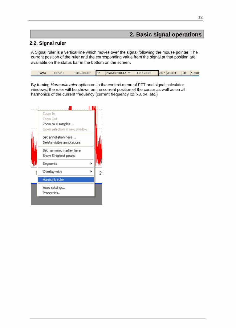
A Signal ruler is a vertical line which moves over the signal following the mouse pointer. Thecurrent position of the ruler and the corresponding value from the signal at that position areavailable on the status bar in the bottom on the screen.
By turning Harmonic ruler option on in the context menu of FFT and signal calculatorwindows, the ruler will be shown on the current position of the cursor as well as on allharmonics of the current frequency (current frequency x2, x3, x4, etc.)
12

2. Basic signal operations
2.3. Signal axes settings
There are two ways to set Y-axis range and position: a fast method by using mouse-wheeldirectly on a signal and a standard method by using Axes settings dialog from the contextmenu.
Fast axes settings by using mouse-wheel
To use the fast Y-axis setting method, move your mouse to the area between the left edge ofthe signal window and Y-axis display. The mouse pointer will change to show a symbol as onthis image:
Turning a mouse-wheel forward will zoom-in the Y-Axis around the current position of thesmall arrow in the cursor pointer. Turning the mouse-wheel in the opposite direction willzoom-out the Y-Axis. Again, the center position for this operation will be position of the smallarrow in the mouse pointer.
If you press Ctrl button during mouse-wheel moving, Y-axis will move up or down instead ofzooming-in or out.
Axes settings by using a dialog
Axes settings for signals can also be performed in Axes settings dialog, which appears afterselecting Edit/Axes settings option or choosing Ctrl+A on active signal window. There areseveral fields in this dialog:
13
2. Basic signal operations
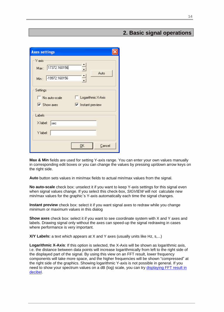
Max & Min fields are used for setting Y-axis range. You can enter your own values manuallyin corresponding edit boxes or you can change the values by pressing up/down arrow keys onthe right side.
Auto button sets values in min/max fields to actual min/max values from the signal.
No auto-scale check box: unselect it if you want to keep Y-axis settings for this signal evenwhen signal values change. If you select this check-box, SIGVIEW will not calculate newmin/max values for the graphic’s Y-axis automatically each time the signal changes.
Instant preview check box: select it if you want signal axes to redraw while you changeminimum or maximum values in this dialog
Show axes check box: select it if you want to see coordinate system with X and Y axes andlabels. Drawing signal only without the axes can speed-up the signal redrawing in caseswhere performance is very important.
X/Y Labels: a text which appears at X and Y axes (usually units like Hz, s,...)
Logarithmic X-Axis: If this option is selected, the X-Axis will be shown as logarithmic axis,i.e. the distance between data points will increase logarithmically from left to the right side ofthe displayed part of the signal. By using this view on an FFT result, lower frequencycomponents will take more space, and the higher frequencies will be shown “compressed” atthe right side of the graphics. Showing logarithmic Y-axis is not possible in general. If youneed to show your spectrum values on a dB (log) scale, you can try displaying FFT result indecibel.
14
2. Basic signal operations
2.4. Overlays
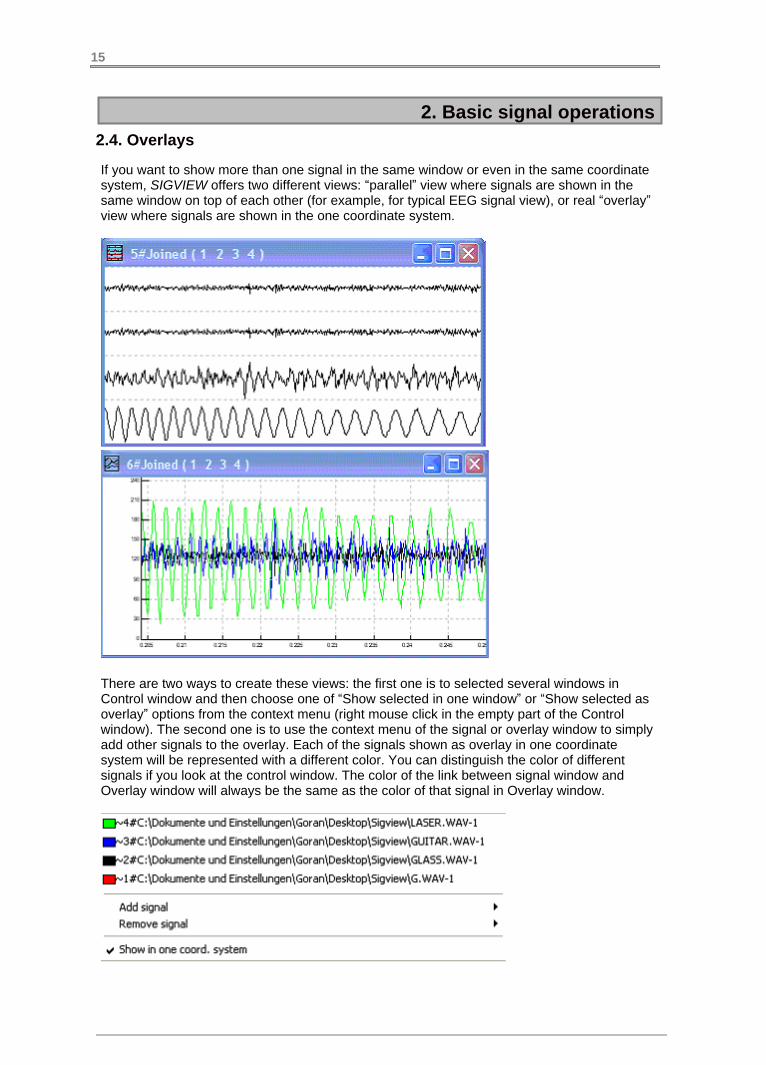
If you want to show more than one signal in the same window or even in the same coordinatesystem, SIGVIEW offers two different views: “parallel” view where signals are shown in thesame window on top of each other (for example, for typical EEG signal view), or real “overlay”view where signals are shown in the one coordinate system.
There are two ways to create these views: the first one is to selected several windows inControl window and then choose one of “Show selected in one window” or “Show selected asoverlay” options from the context menu (right mouse click in the empty part of the Controlwindow). The second one is to use the context menu of the signal or overlay window to simplyadd other signals to the overlay. Each of the signals shown as overlay in one coordinatesystem will be represented with a different color. You can distinguish the color of differentsignals if you look at the control window. The color of the link between signal window andOverlay window will always be the same as the color of that signal in Overlay window.
15

2. Basic signal operations
You can change the order of signals in the Overlay window by pressing Ctrl+Z keyboardshortcut. In “parallel” view, the order of signals will be shifted; in “overlay” view colors of thesignals will be shifted.
You can switch between “parallel” and “overlay” view anytime by pressing Ctrl+S keyboardshortcut.
Note! If windows and their signals have different length or units, SIGVIEW will try to show allof them in the same coordinate system in overlay window - of course, this does not mean thatthe units shown will be valid for all signals. The coordinate system will always be taken overfrom the first signal, the red one. By shifting the signals order with Ctrl+Z keyboard shortcut,you can see the coordinate systems of other signals too.
16

2. Basic signal operations
2.5. Moving through signal and zooming
For advanced zooming and moving through a signal by using a mouse-wheel please seeUsing mouse wheel for zooming and moving through signal.
Zooming signal in & out: Select a part of the signal you want to zoom in and press thezoom-in button on the toolbar or choose a Zoom-in option from the context menu. You canrepeat this as many times you want, and SIGVIEW will memorize your position in signal for
every zoom step you make. You can use the up & down arrow keys or and buttonsin a toolbar to move through your zoom history i.e. zoom in and out of the signal.
Even a faster zoom method is to use your mouse wheel.
Zooming signal to arbitrary length: It is often useful to zoom in a signal to a part whichlength (in samples) is equal to a power of 2. It will have great effect on FFT computation
speed and precision. You can do it by pressing button on a toolbar or choosingEdit/Zoom to X samples/values in the main menu. A dialog will appear with all possible powerof 2 lengths that your signal can be zoomed-in to. Choose the wanted length end press OK.You can also use this option to zoom-in to some arbitrary, non power-of-2 signal length.Simply enter the wanted length in the corresponding edit-box.
Moving through signal: After you zoom in a part of the signal, you can use it to slide throughthe whole signal by using left & right arrow keys. The speed depends on the step value, whichrepresents the percent of the visible part of the signal you move each times you press thearrow key. You can see this value for the currently active signal on the status bar.
Even faster method for moving through signal is to use your mouse wheel.
Step can be changed for the current window by choosing Play&navigate/Step change optionin the main menu or by pressing Alt+Up or Alt+Down keys while signal window has focus.
17

2. Basic signal operations
2.6. Using mouse wheel for zooming and moving through signal
Starting from SIGVIEW v2.0, you can use a mouse-wheel for faster zooming in/out andmoving through signal.
X-Axis
If you simply position signal ruler somewhere in a signal and turn your mouse-wheel forward(away from you), the signal will be zoomed-in to a 20% of its original length. The ruler willremain on the same signal position. Zooming-out can be performed by turning a mouse-wheelin the opposite direction. Please note that these zoom steps will not be saved in a zoomhistory.
There are also two keyboard modifiers which can be used to achieve a special zooming andmoving functions in combination with mouse wheel:
Ctrl key + mouse wheel: Instead of zooming, you will move through the signal by turningmouse wheel. Turning forward will be equal to pressing the left arrow key and turningbackwards will be equal to pressing the right arrow key.
Alt key + mouse wheel: Zooming in/out will be performed as described above, but the lengthof a signal segment in samples will always be a power of 2 (i.e. 1024, 2048,4096,...) for eachstep. It is especially useful for zooming in a signals where FFT function will be performedafterwards.
Y-Axis
To use a mouse wheel to control Y-axis, move your mouse to the area between the left edgeof the signal window and Y-axis display. The mouse pointer will change to show a symbol ason this image:
Turning a mouse-wheel forward will zoom-in the Y-Axis around the current position of thesmall arrow in the cursor pointer. Turning the mouse-wheel in the opposite direction willzoom-out the Y-Axis. Again, the center position for this operation will be position of the smallarrow in the mouse pointer.
Ctrl key + mouse wheel: Instead of zooming, you will move the complete Y-Axis up or down.
18

2. Basic signal operations
2.7. Signal annotations
To label some interesting point in signal or analysis result, you can use signal annotations.Those will be displayed as markers containing some user-specified text and pointing to somesignal location.
You can create annotations by choosing the corresponding context menu option on the signal.Simply position a signal ruler on the location where you would like to define an annotation,press the right-mouse button and choose Set annotation here… menu option. A dialog willappear where you can enter your annotation text of up to 32 characters length.
These annotations will be saved in a workspace file and reloaded later when you load SWSfile. This feature is especially interesting if you want to exchange your signal or analysisresults with somebody and would like your comments to remain visible.
Signal annotations can be deleted by choosing Delete visible annotations option from thecontext menu. If you would like to delete single annotations, simply zoom-in until thatannotation is the only one visible and then choose Delete visible annotations option from thecontext menu.
19

2. Basic signal operations
2.8. VCR-style commands for playing and moving through signal
For a fast navigation and replaying the signal, SIGVIEW provides VCR-like signal navigationfunctions. All functions are accessible from the Play&navigate menu item or in a toolbar:
Rewind: moves to the beginning of the signal
Play (no sound): Moves through the signal just as when you press and hold the rightarrow key. All child windows are recalculated and repainted on each step. There is no soundbeing played. The step for moving through the signal will be a current step for that signal.SIGVIEW will adjust a replay speed to the sampling rate of the signal, i.e. replaying will beperformed in a real-time. If you would like to process signal as fast as possible, selectPlay&Navigate/Play as fast as possible menu option. This option works globally, i.e. will beapplied to all signals after you change it in the main menu.
Play with sound: Plays signal on your sound card and moves through it at the sametime. For example, if you zoom in to a block of 4096 samples length in the signal and use thisfunction, SIGVIEW will play the visible part of the signal, move 4096 samples further, play thenext block etc. until the end of the signal. It is very useful for audio signals because you canobserve the analysis and hear the sound at the same time.
If you try to play the signal and there is no sound, maybe the signal amplitude is simply nothigh enough. SIGVIEW expects signal amplitude values in a 16-bit range, i.e. -32767…32767.If you would like SIGVIEW to automatically adjust signal volume before playing, you can turnPlay&navigate/Adjust volume automatically menu option on.
If you would like SIGVIEW to start playing a signal from the beginning when one of replayoptions arrives signal end, please select Play&navigate/Play repeatedly menu option.
Play visible segment only: Similar as previous function, except that SIGVIEW will onlyplay the visible part of the signal and then stop playing.
Fast forward: moves to the end of the signal
Stop: stops any of the running Play functions
20

2. Basic signal operations
2.9. Extracting parts of the signals
There are two ways to extract a part of the signal into a new window:
1. Edit/Extract signal part (from-to) option from the menu. A dialog appears where you definelimits of the part you want to extract (the units are the same as X-axis units of a signal). A newwindow with extracted part of the signal will appear. It will always contain part of origin signal(for example, 1000-2000Hz part from FFT sequence) that you defined in the Extract dialog. Itis useful for extraction of one part of the spectrum in separate window. You can use it toobserve several frequency ranges in separate windows and calculate their statistics values.
2. Edit/Open selection in new window option from the menu. Select part of the signal andchoose this option from the menu or press Alt+e. A new window with extracted part of thesignal will appear. It will always contain part of origin window which was selected in themoment of creation. It is useful for quickly extracting some visible part of the signal. Forexample, you can select a middle 1/3 of the window. No matter how the content of the originwindow changes (zoom in/out, recalculation), extracted part will always contain the middle 1/3of the origin window, regardless of units or current values on the X-axis.
21

2. Basic signal operations
2.10. Changing signal values
Although SIGVIEW is mainly being used for a signal analysis without changing original signalvalues, it is sometimes necessary to remove some unwanted artifacts from the signal.SIGVIEW offers several functions for altering signal values:
First, you must select the part of the signal you want to change.
By pressing Ctrl+M, all values in the selected part of the signal will be set to the average·(mean) value of the visible part of the signal.If you press Ctrl+0, all values of the selected part of the signal will be set to zero.·
22

2. Basic signal operations
2.11. Exporting window content as image
If you want to save the graphical content of a window as image, use Edit/Copy picture toclipboard from the main menu.
The image will be transferred to the Windows Clipboard as bitmap, and you can paste it toany other picture editing program by choosing its Edit/Paste menu option.
23

2. Basic signal operations
2.12. Working with clipboard
You can use a clipboard to cut, copy or paste parts of the signals, the same way you would doit with the text in any text-processor.
Cutting will be enabled only if you select a part of the signal. If you choose Edit/Cut·
option from the main menu or press button on the toolbar, the selected part of thesignal will be moved to the clipboard (and removed from the signal). You can also use astandard Windows shortcut Ctrl+X for this operation.
If you choose Edit/Copy option from the main menu or press button on the toolbar, a·selected part of the signal will be copied to the clipboard. You can also use standardWindows shortcut Ctrl+C for this operation.
Pasting signals from clipboard will be enabled only if some signal part already exists on·the clipboard. Just put the signal ruler on the position in the signal where you would liketo paste the content of the clipboard and press Ctrl+V. The signal part will be inserted onthat position.
These clipboard functions are meant to be used only internally in SIGVIEW. It is not possibleto use them to exchange signal data with other applications. There is another menu option,Edit/Copy data to clipboard which enables you to copy signal values to the clipboard in a textformat. These data can be pasted as text in any other application, for example MS Excel orMS Word. The data format is the same as in files exported by using ASCII file export options.
24
2. Basic signal operations
2.13. Go to sample function
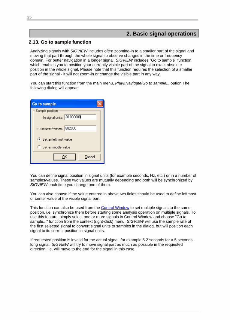
Analyzing signals with SIGVIEW includes often zooming-in to a smaller part of the signal andmoving that part through the whole signal to observe changes in the time or frequencydomain. For better navigation in a longer signal, SIGVIEW includes "Go to sample" functionwhich enables you to position your currently visible part of the signal to exact absoluteposition in the whole signal. Please note that this function requires the selection of a smallerpart of the signal - it will not zoom-in or change the visible part in any way.
You can start this function from the main menu, Play&Navigate/Go to sample... option.Thefollowing dialog will appear:
You can define signal position in signal units (for example seconds, Hz, etc.) or in a number ofsamples/values. These two values are mutually depending and both will be synchronized bySIGVIEW each time you change one of them.
You can also choose if the value entered in above two fields should be used to define leftmostor center value of the visible signal part.
This function can also be used from the Control Window to set multiple signals to the sameposition, i.e. synchronize them before starting some analysis operation on multiple signals. Touse this feature, simply select one or more signals in Control Window and choose "Go tosample..." function from the context (right-click) menu. SIGVIEW will use the sample rate ofthe first selected signal to convert signal units to samples in the dialog, but will position eachsignal to its correct position in signal units.
If requested position is invalid for the actual signal, for example 5.2 seconds for a 5 secondslong signal, SIGVIEW will try to move signal part as much as possible in the requesteddirection, i.e. will move to the end for the signal in this case.
25

2. Basic signal operations
2.14. Signal display options
SIGVIEW includes various options for signal displaying. Those are accessible for each signalwindow from its context menu or from a toolbar.
Default signal display type (line of single width) is by far the fastest way for displaying signalsand should be used always if speed is important.
There are 4 different display types:
Line: signal will be shown as a line connecting actual signal values
Histogram (Zero reference): For each signal value, a vertical rectangle will be drawn startingon the value of 0. This is useful if signal does not have too many values, for example for aprobability distribution graph.
26

2. Basic signal operations
Histogram (Min reference): Very similar as Zero reference histogram graphics, but eachrectangle will be drawn from the minimal value of the signal and not from the 0.
Area: With this display option, the area between a signal line and zero line will be filled.
Dots: A single dot will be drawn on a position of each signal value
27

2. Basic signal operations
Show dots option can be used in a combination with Line, Histogram and Area display typeto show dots on samples positions additionally to a standard display:
As a combination with the "Line" display type, a line width can be chosen as single (default),double or triple line-width.
28

2. Basic signal operations
29

PartLoading and saving
Sigview User Manual
III

3. Loading and saving
3.1. Loading and saving signals
Loading signals: After you select File/Open signal option from the menu or the buttonfrom the toolbar, the Open signal dialog will appear. In this dialog, you can choose a file typeand the name(s) of the file(s) you want to load in SIGVIEW.You can also use drag 'n drop to drag one or more files from Windows Explorer and dropthem on SIGVIEW window. The effect will be the same as if loading these files through Openfile dialog.
Loading compressed signals: Compressed signal file formats like MP3 or WMA require aspecial decoder component to be opened (codec). These components are not included inSIGVIEW, but are most probably already installed in your system. SIGVIEW uses MicrosoftDirectX technology and codecs already installed in your system for file decompression. Thatensures that any file playable on your computer (for example in Windows MediaPlayer) willmost probably also be readable by SIGVIEW.
Loading very long signals: Since SIGVIEW loads the complete signal in RAM memory ofyour computer, a maximal size of one signal will be around 300-500MB. This is usually thelimit for allocating one continuous memory block under MS Windows. This is equal to~30-40min of 16-bit signal at 48kHz. If you try loading a longer signal, SIGVIEW will reportthat it can not allocate enough memory for it and offer you to load a smaller part of the signalwhich can fit in memory.
Saving signals: You can save a signal if you choose File/Save signal as… option or the toolbar button. SIGVIEW can save signals in WAV format (16-bit integer or 32-bit float) orexport them as ASCII or raw binary file. Saving signals to a WAV file is possible only forsignals with integer sampling rate. Also, please note that a 16-bit WAV format supports onlyinteger sample values - it means that all values from your signal will be rounded before savingthose in a WAV file. If you do not want this to happen, you can save your signal in a 32-bitfloating point WAV format. You can save only the visible (currently zoomed-in) part of thesignal by using “Save visible signal part as…” menu option. For saving multi-channel signals,please see Saving multi-channel signals chapter.
Replacing the file: If you want to perform the same analysis on several similar signals, thereis an easy way to do it: you can create the complete analysis system for the first signal andreuse it for all others. Just replace the signal with some other signal by choosing File/Replacewith... option from the menu and observe the results. The only restriction is that both originaland replacement files must have the same length and the sample rate.
ASCII files: By using main menu options File/ASCII files/... You can also export/import signalsin a standard tab, comma or semicolon separated ASCII format. Here is an example of TABdelimited file:
X value<TAB>Y value channel1<TAB>Y value channel 2<TAB>...Y value channel N<newline>X value<TAB>Y value channel1<TAB>Y value channel 2<TAB>...Y value channel N<newline>X value<TAB>Y value channel1<TAB>Y value channel 2<TAB>...Y value channel N<newline>X value<TAB>Y value channel1<TAB>Y value channel 2<TAB>...Y value channel N<newline>....................................................................
31

3. Loading and saving
There are also a separate menu options for loading ASCII files using dot as decimal separator(default) and comma (used in Europe).
When you export your signal to a ASCII format from SIGVIEW, there are two optionsavailable: Export signal (X/Y values) will export both X and Y values and Export signal (Yvalues) will export only Y values.When loading ASCII files, SIGVIEW will try to analyze the first data column to see if it can beused as X axis values (if values are equidistant). If yes, you will be asked if you would like touse the calculated sampling rate for the loaded signal. If the calculation was not 100% correctbecause there were not enough data in the file, you can still accept this value and change itlater through the Edit/Sample rate change menu option.
For saving multi-channel ASCII files, please see Saving multi-channel signals.
Please note that SIGVIEW saves only a visible (zoomed-in) part of the signal. If you want tosave the whole signal, use the zoom-out option first. If you have your data already loaded insome other application, for example Microsoft Excel, the ASCII file format would be theperfect file format for data exchange. Just save your data in the other application astab-delimited TXT/ASCII file, and import it in SIGVIEW afterwards.
Exporting 3D graphics values in file: By using main menu option File/ASCII files/Export3D-graphics, you can export all values from the visible part of the 3D graphics in one text file.There are 3 options: export in a file with X,Y,Z triples in 3 columns (tab delimited), export amatrix where first row contains X values, first column Y values and the rest of the file are Zvalues (tab delimited) and finally inverted variant of the second matrix format (with switchedrows and columns). All of these file types can be loaded by, for example, MS Excel for furtheranalysis.
32

3. Loading and saving
3.2. Saving multi-channel signals
Saving multi-channel signal can be performed by using Control Window.
First step is to find icons in Control Window corresponding to the channels of the signals youwould like to save and selecting them in the right channel order. Next to the each selectedicon, a selection order will be shown (1,2,...). It will correspond to the channel order in a savedfile.
After selecting all channel in the right order, open context menu (right mouse button in theempty part of a Control Window).
33

3. Loading and saving
The following options will be available if all selected signals are suitable for saving in one file(see below):
- Save selected signals as: Saves selected signals in a WAV file (16-bit integer or 32-bitfloat)
- Save visible part of selected signals as: Saves only a currently visible part of eachselected signal in a file
- Export selected signals in ASCII file (X/Y values): Saves selected signals in an ASCII fileincluding X/Y values. X-axis values from the first channel will be used.
- Export selected signals in ASCII file (Y values only): Saves selected signals in an ASCIIfile. Only signal amplitude values will be saved.
In order to save multiple channels in one file, all channels must have the same sampling rate(i.e. distance between samples). Furthermore, if the signals have different lengths, the longerones will be saved only up to the length of the shortest one.
34
3. Loading and saving
3.3. File formats
See also general topics about loading and saving signals.
Standard SIGVIEW version can read signals stored in several different file formats:
*.WAV files
Standard Wave audio format (8, 16, 24 or 32-bit) including compressed WAV files ifcorresponding codecs are installed in the operating system.
Compressed file formats
Use File/Open signal… menu option. You will be able to open most compressed file formatslike compressed WAV files, MP3, WMA, ASF etc. SIGVIEW will use Microsoft’s DirectShowand installed codecs for the file decompression. That ensures that any file playable on yourcomputer will also be readable in SIGVIEW. Please note that file decompression can be arather slow operation, and the resulting signals can be very long.
Audio Interchange File Format (.AIF, .AIFC, .AIFF)
SIGVIEW uses DirectX services for loading these files. Therefore, a Windows Media Playerv7 or higher is required.
Sun Microsystems and NeXT audio files (.AU,.SND)
SIGVIEW uses DirectX services for loading these files. Therefore, a Windows Media Playerv7 or higher is required.
ASCII files
Available through ASCII Import/Export options in File menu. The ASCII files have to be in afollowing format (choose appropriate option if your files use comma as decimal separator):
X value<TAB>Y value channel1<TAB>Y value channel 2<TAB>...Y value channel N<newline>X value<TAB>Y value channel1<TAB>Y value channel 2<TAB>...Y value channel N<newline>X value<TAB>Y value channel1<TAB>Y value channel 2<TAB>...Y value channel N<newline>X value<TAB>Y value channel1<TAB>Y value channel 2<TAB>...Y value channel N<newline>
Raw binary files
Available through File/Raw binary files/Export and Import menu options. Raw binary files aresimple binary arrays of samples, saved in one of these supported formats:
8-bit signed8-bit unsigned16-bit signed16-bit unsigned32-bit float
35

3. Loading and saving
Only one signal (channel) can be loaded from one raw binary file.
EDF (European File Format)
The European Data Format (EDF) is a simple and flexible format for exchange and storage ofmultichannel biological signals. EDF was developed by a group of European medicalengineers and published in 1992 in Electroencephalography and Clinical Neurophysiology 82,pages 391-393. Since then, EDF became a de-facto standard for EEG and PSG recordings incommercial equipment and multicenter research projects. You can find further informationabout this format at: http://www.hsr.nl/edf
36

3. Loading and saving
3.4. Loading and saving workspaces
By using “Load Workspace...” and “Save workspace...” options in a File menu, you can saveall currently opened SIGVIEW windows and their relations ( a "Workspace") in a file andreload it later.
Concept
SIGVIEW does not save the actual content of each signal or analysis result – it saves only astructure of your analysis system and a file names for loaded files. For example, if you load asignal, perform an FFT on it and save that workspace, SIGVIEW will not save the actualvalues from the signal or values from the FFT result. Only the name of the signal file will besaved along with the information that you performed FFT on it with certain parameters.Therefore, if you change the data in the original signal file and reload SIGVIEW workspace,you will get changed signal data and the FFT from it. Generally, a workspace file contains theinformation you can normally see in a Control Window plus properties for each windowincluding axes properties and zoom info.
Files
SIGVIEW is saving its workspace in a file with extension SWS (SIGVIEW WorkSpace). Thisfile is a plain text file with the structure similar to Windows *.INI files. Its structure is quitesimple and easy to understand or even to edit manually. You can open SWS file with any texteditor and perform some changes if you need it. You can even edit its content automaticallyfrom another application to control SIGVIEW functionality.
For all loaded signals, SIGVIEW saves their full path names in workspace file. When openingthat workspace file later, SIGVIEW searches for those files on their original location first (forexample c:wav). If file does not exist, SIGVIEW tries to load the file with the same name fromthe folder where SWS file is. Therefore, if you want to distribute workspace file with all thesignals needed, you just have to be sure that the SWS and signal files will be in the samefolder on target computer.
Information about window location and size will also be saved for every window. Thisinformation is relative to the size of the main SIGVIEW window, so you can be quite sure thatthe loaded workspace will look the same way in every screen resolution or SIGVIEW windowsize.
It is also possible to create a workspace file without defining exact signal file names in it.When opening such workspace file, SIGVIEW will ask you for a file name for each signal fileused in this workspace. To create such workspace file, just save it once normally – with filenames, then open the SWS file with any text editor program and replace all file names in it (allFileName=.... keys) with “FileName=choose”.
You also use drag 'n drop to drag one or more Workspace files from Windows Explorer anddrop them on SIGVIEW window. The effect will be the same as if loading these files by using"Load Workspace..." menu option.
37

3. Loading and saving
Using Workspace file as a command line argument
It is possible to give an SWS file as a command line argument when starting SIGVIEW, forexample:
SIGVIEW32.EXE c:\myworkspace.sws
SIGVIEW will start and open this workspace. It is also possible to define all needed signal filenames in the command line as well. You have to create the SWS file where each signal filename is replaced with “#X”, where X=1,2,3,..., for example “FileName=#1”. Then you can startSIGVIEW with
SIGVIEW32.EXE c:\Analysis1.sws c:\file1.wav c:\file2.wav
Every appearance of “#1” in the Analysis1.sws will be replaced with “c:\file1.wav”, everyappearance of “#2” with “c:\file2.wav”, and so on....
Saving file names in a Workspace
If you are saving a Workspace (SWS file) containing windows with file-based signals (forexample, loaded WAV files), SIGVIEW will offer you two options:
1. Save full file names in a file: Each time you load the workspace, your files (if they still exist)will be automatically loaded. The result will be exactly the same as the workspace you savedif those signal files did not change in the meantime.
2. Do not save file name information in a file: Saved workspace will be used as a template foroperations on any files. Each time you try to load the workspace, SIGVIEW will offer you a fileload dialog to choose a file which should be loaded for each window from the workspacewhich contained file-based signal. This can be used to speed up the analysis you have toperform often on different files, similar to Custom tools.
Examples
Several example workspace files are installed in “Examples” subdirectory of SIGVIEW'sapplication data directory (usually C:\Documents and Settings\<UserName>\ApplicationData\Sigview\) and can be accessed directly through Help/Examples... option in the mainmenu.
38

3. Loading and saving
3.5. Creating and reusing custom tools
By using “Save window as custom tool” and “Apply custom tool...” options from the File orSignal tools menu, you can save parts of your analysis graphs and reuse them later as yourcustom tools.
Creating new tools
There are two options for saving a tool: First one is to save only one window as a tool with allits properties. For example, if you performed FFT from a signal and changed some FFTproperties: smoothing, removing linear trend.... You can save all those settings as a singleFFT tool by clicking on FFT window and choosing “Save window as custom tool -> Windowonly...” option from the menu. Save dialog appears where you can define a name for your toolfile – for example “MyFFT.swt”. Only the information about the tool type (FFT) and itsproperties will be saved. Now, you can load any other signal and choose “Use custom tool>”from the menu. If you have saved your tool in a default “Sigview” folder, its name will appearin a submenu. Otherwise, choose “From file…” option, find “MyFFT.swt” file and open it. FFTwill be performed on your signal, exactly with the properties you saved earlier. The sameprinciple is applicable to all SIGVIEW functions including 3D analysis and instruments.
Second option when saving tools is to use “Save window as custom tool -> Window and itssubtree...”. This option will save active window and all its child windows as a one tool. Forexample, you can perform FFT analysis, and then use “Instruments... Maximum position”function to display dominant frequency from the FFT. If you save the FFT window with itssubtree as a new tool, the instrument window will also be saved. If you apply this saved tool tosome signal, you will get its FFT with originally saved settings, and an instrument showing themaximum value from the FFT. With this option, you can save very complex tools includingdozens of connected windows.
Default folder for saving and loading custom tools is “Tools” folder located under the folderwhereSIGVIEW is installed. After you install SIGVIEW, there are already few example tools there.
Using tools
When using a custom tool, SIGVIEW will try to check if the tool is applicable to the currentlyselected window. For example, if you extract a part of some signal between its 5th and 6thsecond and save that extraction window as a tool, it will not be applicable to the signals withonly 3 seconds of length.
You can also use drag 'n drop to drag SWT files from Windows Explorer and drop them inSIGVIEW. Those will be applied to the currently active SIGVIEW window.
You can also include your custom tools into the SIGVIEW's toolbar and assign them todedicated toolbar buttons. If you click on the "T..." button in the "Custom tools" toolbar part, adialog will open allowing you to assign a tool (SWT file) to each of 5 custom buttons labeledT1...T5.
After you assign a tool to a button, the button will become enabled and allow you to apply thecorresponding tool with a single click instead of searching and opening the SWT file first.
39

3. Loading and saving
Further reading
Also, please see the chapter about Drag 'n Drop in Control Window. It describes some similaralternative functions for reusing parts of the analysis without saving those into SWT files first.
For more detailed examples on custom tools usage, please see How-To example.
40

PartControl window
IV

4. Control window
4.1. Control window basics
Control window enables you to work easily with many signals or analysis windows at thesame time. Each signal, analysis window, 3D graphics or instrument created while workingwith SIGVIEW is represented with its icon in a Control window.
Icons are connected with solid lines to show a signal flow through the system. A dotted lineshows that signal link is not active and changes in the parent will not cause child window torepaint.
Selecting in Control window
You can select or unselect icons by clicking on them with the left mouse button. Everyfunction you perform in the Control window (for example FFT, Time-FFT, Extract from-to,...)refers to selected icons, i.e. windows they represent. For faster selecting or unselecting, clickright mouse button in the empty part of the Control window and choose some of the selectingoptions from context menu (Select all, Unselect all, Invert selection,...).
Operations on single windows
Click right mouse button over some icon and a context menu will appear with some importantfunctions for the window it represents. If you choose one function from the menu, the resultwill be just as if you have chosen that option for the window itself.
42
4. Control window
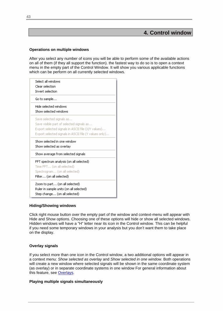
Operations on multiple windows
After you select any number of icons you will be able to perform some of the available actionson all of them (if they all support the function). the fastest way to do so is to open a contextmenu in the empty part of the Control Window. It will show you various applicable functionswhich can be perform on all currently selected windows.
Hiding/Showing windows
Click right mouse button over the empty part of the window and context-menu will appear withHide and Show options. Choosing one of these options will hide or show all selected windows.Hidden windows will have a "H" letter near its icon in the Control window. This can be helpfulif you need some temporary windows in your analysis but you don’t want them to take placeon the display.
Overlay signals
If you select more than one icon in the Control window, a two additional options will appear ina context menu: Show selected as overlay and Show selected in one window. Both operationswill create a new window where selected signals will be shown in the same coordinate system(as overlay) or in separate coordinate systems in one window For general information aboutthis feature, see Overlays.
Playing multiple signals simultaneously
43
4. Control window
You can also use VCR-like functions on multiple signals selected in the Control window. It willallow you to play more signals at the same time and simulate real-time comparison orcombination between them. If your sound card supports that feature, you will be able to hearboth signals mixed at the same time.
Calculating Average from two or more signals
There is also a special functionality of the Signal averager window when used from theControl window. To use it, select two or more signals in the Control window and chooseSignal tools/Averager context menu option. A new signal window will be created, representingaverage value from all selected signals.
44
4. Control window
4.2. Linking & unlinking windows
Two windows are "linked" in SIGVIEW if changes in one of them influence the changes in theother one. For example, if you calculate an FFT sequence from some part of the signal, thatFFT will recalculate and redraw each time you move through the original signal, zoom it in orout, change signal values, ...
All windows except Time FFTs are by default linked to its parent windows. You can disable
that link by choosing System control/Unlink window from parent menu option or button ina toolbar. You can establish that link again by choosing System control/Link window to parent
menu option or button in toolbar.
You can see the current state of links between windows in the Control window. If two windowsare linked, they will be connected with a solid line. If they are not linked, the line will be dotted.You can also perform linking/unlinking from the Control window’s context menu.
45

4. Control window
4.3. Drag 'n Drop functions
The fastest way to reuse/copy parts of your current Workspace or to apply an existinganalysis sequence to some existing window is to use Drag 'n Drop functions in the ControlWindow. Here are some usage examples:
Reusing or moving part of analysis
By dragging an analysis window icon to some other target window icon in the Control Window,the complete analysis tree starting from the dragged window icon will be copied and applied tothe target window. If Ctrl-key is pressed, the analysis tree will be moved, otherwise it will becopied. The cursor shown during dragging will indicate the current mode by displaying"COPY" or "MOVE" text next to the graphics.
And here is a simple example. The starting point would be this workspace:
We perform drag operation of the FFT window to the new Signal2:
And the result is that the copy of the analysis is applied to the Signal2:
46

4. Control window
The current drag context can be recognized on the cursor mouse cursor shape:
Currently dragged window and its subtree will be copied - there is no specific target toapply it to. Applicable only to root windows (without parent).
Currently dragged window and its subtree will be copied and applied to the window iconcurrently under mouse cursor.
Currently dragged window and its subtree will be moved - there is no specific target toapply it to. Applicable only to root windows (without parent).
Currently dragged window and its subtree will be moved and applied to the window iconcurrently under mouse cursor.
Duplicating existing analysis parts
By dragging the icon of the root window (window without parents) to the empty space in theControl Window, the copy of that window and its analysis subtree will be created.
Dragging Tools file (*.SWT) onto Control window
It is also possible to use drag 'n drop between Windows Explorer and Control Window. If youdrag a saved Tool file (*.swt file) from Windows Explorer to the Control Window inside
47

4. Control window
SIGVIEW, that tool will be applied to all currently selected windows in the Control Window.
48

PartSignal analysis
V
5. Signal analysis
5.1. FFT
Most of spectral analysis tools in SIGVIEW are based on the FFT algorithm. Its main purposeis to transform the signal from its time-domain representation into the frequency-domainrepresentation. For the detailed mathematical description of the algorithm and itsinterpretation, please refer to the following internet resources:
http://en.wikipedia.org/wiki/Fast_Fourier_transform
http://www.fftw.org/links.html
http://astronomy.swin.edu.au/~pbourke/analysis/dft/
http://www.eptools.com/tn/T0001/INDEX.HTM……..
And a wonderful web page with a free book on digital signal processing:
http://www.dspguide.com/
By preparing a signal before using the FFT algorithm, changing FFT calculation parameters orpost-processing its results, many different variations of the FFT transformation can beapplied. One of the most important features in SIGVIEW is the possibility to change most ofthese parameters and easily observe and compare the results.
To apply FFT transformation to your signal in SIGVIEW, select some window containing asignal and choose Signal tools/FFT option. An FFT result window will be created containingthe FFT result calculated according to your current Spectral analysis defaults. You canchange the parameters for the already calculated FFT sequence anytime by choosingEdit/Properties option from the main menu or Properties option from the context menu. Thedialog for the editing of FFT parameters is the same as the Spectral analysis defaults dialog –you can find the detailed description of its fields here.
50

5. Signal analysis
5.2. Spectral analysis defaults
Most of spectral analysis tools in SIGVIEW are based on the FFT algorithm. There are manydifferent parameters which can be applied to the signal before the FFT analysis is performed,to the FFT calculation itself or its result.
If you want to change the default settings for spectral analysis calculation in SIGVIEW, useSignal tools/Spectral analysis defaults option from the main menu. These settings will beapplied to all new FFT-based calculations, including FFT, Time-FFT, cross spectral analysis,etc.
Once the FFT or Time FFT is already calculated according to your current spectral analysisdefaults, you can edit those anytime by choosing Edit/Properties menu option for calculatedwindow (FFT, Time FFT,…). The same option is also available in the window’s context menu.These settings will apply only to that single window.
The following parameters can be changed for each FFT based spectral analysis operation inSIGVIEW:
Subtract mean check box: Select it if you want to normalize the signal before processing. Itsimply subtracts the mean value of the signal from each sample
51

5. Signal analysis
Remove linear trend check box: If linear trend appears in signal ( i.e. the whole signal raisesor falls monotonously), it can affect evaluation of low frequency components in the FFT. Thisoption removes linear trend by subtracting linear least squares approximation from the signal
Remove values > : This option automatically removes values from the signal that are not inrange ( mean -N*StDev , mean + N*StDev ) where StDev is a standard deviation of the signaland N is a user-defined coefficient entered in the corresponding edit box. Values are removedby replacing them with the mean value.
Apply window: To avoid some undesirable effects of discrete Fourier transform, it isrecommended to lower the signal values near the end of the signal by multiplying it with someappropriate weighting function. This technique is called “windowing”. SIGVIEW supportsseveral standard weight functions: Hann, Haming, Blackman, Triangle, Tukey. Choosing“Rectangle” window has the same effect as turning windowing option off.
Zero padding: Due to the nature of the FFT algorithm, the fastest calculation will beperformed for signals having power-of-2 length (for example 128, 256, 512,…). If your signalor the part you would like to analyze have some other length, there are several options youcan choose:
Never use zero padding: FFT or slower DFT algorithm will be applied on your·signal without altering or extending it with zeros. This is the slowest calculationmethod, but the advantage is that your signal is not changed in any way. Forprime number signal lengths the calculation will be performed by using very slowDFT algorithm.Optimal method: Your signal will be expanded with zeros to the next possible·length allowing the usage of the FFT algorithm instead of very slow DFT.Next power of 2: Your signal will be expanded with zeros until the next·power-of-2 length. This will enable the usage of fastest FFT algorithm.
To increase the precision of the spectral analysis without taking longer signal segments, youcan also expand existing signal segment with zeros, even beyond the next power-of-2 length.That will not add essentially new information in the FFT result, but will increase its precision,i.e. will reduce the size of the one frequency bin. You will simply get FFT result with morepoints - from the same signal segment. (If signal has 1024 samples and you chooseexpanding by factor 8, resulting spectrum will have 4096 pt. instead of 512 without usingoption). The result will be comparable to interpolation of the normal FFT result. To use thisfeature, you can choose 2x, 4x or 8x zero padding option.
Spectrum type:
Instantaneous spectrum (no averaging): Each change in the signal will cause·the FFT to recalculate. This is the default behavior.
Average last X spectrum results: This option is useful only for the FFT of the·live input signal or other fast changing signals. Last X complex FFTs will beaveraged to calculate the final result. That will decrease the influence of the noisein the signal and is usually recommended for all spectral analysis functions on thelive signal.
Show result as: After applying the FFT algorithm to the signal, the result will be an array ofcomplex numbers. These radio-buttons determine the way these complex numbers will be
52

5. Signal analysis
converted to real values and displayed as FFT graphics.
Magnitude: value generally regarded as “spectrum”; calculated as sqrt(R^2 + I^2)·Power spectrum: Magnitude squared.·Power spectral density (PSD): Power spectrum is calculated first and its values are·divided with the width of the frequency bin. This “normalization” makes comparisonsbetween FFT sequences from different signals with different sampling rates possible.Phase: show signal phase angle (in degrees)·Real & Imaginary part: show only real or only imaginary part of the spectrum·
Apply custom filter curve: You can apply custom filter curve to change the values of thespectrum. See Custom filter curves section for more information. This option is applicable onlyto magnitude and power spectrum result types.
Logarithmic Y-Axis (dB units) option can be applied only to Magnitude, Power spectrumand PSD spectrum results. It shows a logarithmic values for all FFT result points, causingY-axis to be logarithmic.
Y-axis in dBFS: This option can be applied only if Logarithmic Y-Axis is used. It will calculatedB values relative to some maximal, i.e. full scale value. You can freely define this Full-scalevalue in signal units (for example 32767 for 16-bit sound card or max. voltage for NiDAQdevice). There is also a combo-box with the choice of some predefined values for the maximalamplitude. If you set the full scale value to 0, dB values will always be calculated relative tothe currently highest FFT value so that the highest value is always equal to 0 dB and all otherFFT values are negative.
X-Axis units combo box: allows you to switch between following X-axis units: “Hz(Cycles/sec)”, “CPM (Cycles/minute)”, “KHz”, “MHz”.
Smoothing: If the result of FFT is noisy and has many values, it can be useful to smooth it byusing weighted moving average function. That will remove small noisy details from the FFTand give you a better overview of the important spectrum events. You can choose some ofstandard weighting functions here and determine the length of a smoothing window (longerwindow means more smoothing).
Test for confidence: Siegel’s test for confidence of spectral peaks tells you if some peak inspectrum is statistically significant or it could be product of some random fluctuation of thesignal. If you turn this option on, only significant peaks will be shown, while all other values inthe spectrum will be set to zero. You can choose two levels of confidence for this test: 95% or99%. This test is purely statistics; it does not use any artificial intelligence methods.
53
5. Signal analysis
5.3. Signal calculator
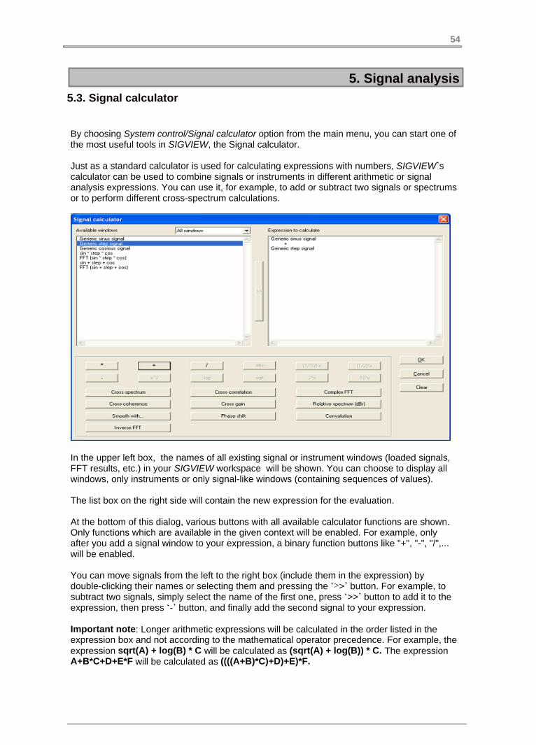
By choosing System control/Signal calculator option from the main menu, you can start one ofthe most useful tools in SIGVIEW, the Signal calculator.
Just as a standard calculator is used for calculating expressions with numbers, SIGVIEW’scalculator can be used to combine signals or instruments in different arithmetic or signalanalysis expressions. You can use it, for example, to add or subtract two signals or spectrumsor to perform different cross-spectrum calculations.
In the upper left box, the names of all existing signal or instrument windows (loaded signals,FFT results, etc.) in your SIGVIEW workspace will be shown. You can choose to display allwindows, only instruments or only signal-like windows (containing sequences of values).
The list box on the right side will contain the new expression for the evaluation.
At the bottom of this dialog, various buttons with all available calculator functions are shown.Only functions which are available in the given context will be enabled. For example, onlyafter you add a signal window to your expression, a binary function buttons like "+", "-", "/",...will be enabled.
You can move signals from the left to the right box (include them in the expression) bydouble-clicking their names or selecting them and pressing the ‘>>’ button. For example, tosubtract two signals, simply select the name of the first one, press ‘>>’ button to add it to theexpression, then press ‘-’ button, and finally add the second signal to your expression.
Important note: Longer arithmetic expressions will be calculated in the order listed in theexpression box and not according to the mathematical operator precedence. For example, theexpression sqrt(A) + log(B) * C will be calculated as (sqrt(A) + log(B)) * C. The expressionA+B*C+D+E*F will be calculated as ((((A+B)*C)+D)+E)*F.
54

5. Signal analysis
When you create the complete signal expression, click OK to create the result signal. It will belinked to all windows included in the expression and will recalculate and redraw each timethey change. In case that one of expression windows is deleted, the calculator window will befrozen and will keep its last values.
Unary functions (can be applied to the on signal or instrument window)
sqrt (square root)·log (log10)·x^2 (squared)·abs (absolute value)·2* (multiply with 2)·10* (multiply with 10)·(1/2)* (multiply with 1/2 i.e. divide with 2)·(1/10)* (multiply with 1/10 i.e. divide with 10)·
Binary functions (can be applied to two signal or instrument windows)
* (multiply)·/ (divide)·+ (plus)·- (minus)·
Cross-correlation·Convolution (convolutes first signal with the second one)·Smooth with (smooth first signal by using the second one as a·weighting function)Cross spectrum·Cross coherence·Cross gain·Phase shift·Relative spectrum (dBr) Complex-FFT·Inverse-FFT·Complex-FFT·
If only a simple arithmetic binary functions (*, /, +, -) are used, you can freely mix instrumentand signal windows in the expression.
If you include two signals of different lengths in a binary operation (for example you subtractone signal from another one), SIGVIEW will use only a part of the longer signal (starting fromits first sample) which has the length of the shorter signal.
Examples
Here are some examples of calculator expressions.
55

5. Signal analysis
1. Simple arithmetic operation on spectrums.
You have loaded two signals, calculated their spectrums and you have the followingworkspace:
Now, you would like to subtract two calculated spectrums to get some information about theirdifferences. To do it, create the following expression in the Signal calculator:
The resulting window will contain th requested difference between spectrums.
2. Combining instruments and signals in one expression
You would like to subtract mean value of a signal from all signal values (normalization). First,you would calculate signal mean by using the appropriate instrument:
56

5. Signal analysis
Then, you would create the following expression in the Signal calculator:
The result will be a new signal calculated as requested:
2. Instrument-only expressions
You can also have expressions containing only instrument windows. The result of suchexpressions will also be a new instrument window.
In this example, we calculate RMS of two signals and then create a new instrument containingtheir difference:
3. Complex expressions
There a practically no limitations for creating calculator expressions. Here are someexamples:
f = A^2 + abs(B) - B^2
57

5. Signal analysis
Subtract spectrum of one signal from its cross spectrum with another signal
Calculate log-values of both real and imag spectrum and then perform inverse FFT
58

5. Signal analysis
5.4. Autocorrelation
Accessible through Signal tools/Autocorrelation menu option.
Autocorrelation is a tool used frequently for the analysis of time domain signals. It is thecross-correlation of the signal with itself. Autocorrelation is useful for finding repeatingpatterns in a signal, such as determining the presence of a periodic signal which has beenburied under noise, or identifying the fundamental frequency of a signal which does notactually contain that frequency component, but implies it with many harmonic frequencies.
The same function can be performed in Signal calculator by performing the cross-correlationof the signal with itself.
59

5. Signal analysis
5.5. Filters
Filtering is the operation which removes or changes specific frequency components from thesignal. In SIGVIEW, you can simply apply a filter to the signal by defining frequency segmentto be removed, or the segment you want to leave in the signal. That way, you can createbandstop, bandpass, highpass and lowpass filters.
When you choose Signal tools/Filters option from the main menu, a dialog appears where youcan enter segment boundaries (in Hz) and determine if you want to remove that frequencysegment (bandstop), leave only that frequency segment (bandpass) or you want to remove allfrequencies up to (highpass) or above some frequency (lowpass).
For Bandstop and Bandpass filter types, you can also include all higher harmonics of definedfrequency segment. If the defined segment is [x,y], it will also include all segments [N*x, N*y],where N=2..Nmax.
There is also an option to use custom filter curves for signal filtering. For details, please seeCustom filter curves section.
After pressing OK, a new window with filtered signal will appear. You can change filter’sfrequency boundaries later by choosing Edit/Properties on filtered signal window from themenu. You will be able to see instantly how these changes affect the filtered signal.
SIGVIEW uses FFT-based filtering algorithm. It is a combination of the FFT calculation,changes in the FFT result (filling some frequency bands with zeros or applying custom filtercurve) and the inverse FFT calculation. This method is relatively slow compared to otherfiltering methods, but is usually very accurate.
60

5. Signal analysis
5.6. Signal averager
Signal Averager is a signal that calculates average values of all past changes in its parentsignal.
For example, try to make Averager window of some existing spectrum window. WhenAverager is created, it contains exactly the same data as the current spectrum. Now, startyour analysis system and make spectrum values change. Averager ‘catches’ all changes ofthe spectrum and calculates their average. This way, you will get a spectrum average throughtime. You can apply this option to any kind of signal.
If you want to reset all averager values and start with the averaging again, choose Reset datafrom its context menu.
If you want simply to stop or start averaging process, choose unlink or link option from themain menu or toolbar.
61

5. Signal analysis
5.7. Resampling signals
Accessible through Signal tools/Resample menu option.
Resampling is a process of changing sampling rate of an existing signal. A new signal shouldkeep as much as information contained in the original signal as possible.
A resampling dialog in SIGVIEW lets you choose a new sampling rate for the signal andshows you a resampling factor (a ratio between new and old sampling rates). This factor mustbe in the range [0.1, 10], i.e. you can increase (up-sampling) or decrease (down-sampling)sampling rate by the factor of 10.
For some combinations of the current and new sampling rates, SIGVIEW will not be able toachieve exactly the requested new sampling rate. For example, when converting 44.1 kHzsignals to 48 kHz signals, SIGVIEW will generate a signal with the sampling rate of48000.00114 Hz. This is caused by the underlying algorithm.
As all SIGVIEW functions, resampling is performed only on visible part of the origin signal.Any change in the origin signal, for example zooming in/out will cause the resampled signal tobe recalculated.
62

5. Signal analysis
5.8. Remove DC offset
Accessible through Signal tools/Remove DC offset menu option.
This option normalizes your signal by subtracting signal's mean value from all signal'samplitude values. The result is a signal with the mean equal to zero.
This operation should always be performed before using Signal tools/Integrate option.
63

5. Signal analysis
5.9. Moving average smoothing
Smoothing is the operation that can very often help to extract some useful information from anoisy signal or indistinct FFT sequence. The overall effect of smoothing is similar to filteringwith the lowpass filter.
In SIGVIEW, smoothing is performed by using weighted central moving average method. InSmoothing dialog you can determine the type of weighting function to be used and its length.Longer function will provide stronger smoothing effect on the signal.
If you want this operation to be performed on each FFT result after its calculation, you canturn it on in Spectral analysis defaults .
You can change the smoothing parameters for a smoothing window if you openEdit/Properties menu option from its context menu.
64
5. Signal analysis
5.10. Removing linear trend
If linear trend appears in the signal (i.e. the whole signal raises or falls monotonously), it canaffect the calculation of low frequency components in the FFT. With the help of Signaltools/Remove linear trend option, you can transform the origin signal to a new signal withoutlinear trend. That signal can be used for further analysis. Linear trend will be removed bysubtracting signal’s linear least squares approximation from the original signal.If you want this operation to be performed before each FFT calculation, you can set it inSpectral analysis defaults .
65

5. Signal analysis
5.11. Cross-spectral analysis
Cross-spectral analysis gives you information about relations between two signals in theirfrequency domain. All cross analysis functions are accessible through Signal calculator .Several functions are available:
Cross-correlation: measure of similarity of two signals, commonly used to find features in anunknown signal by comparing it to a known one. It is a function of the relative time betweenthe signals. It can also be used to detect similarities in possibly time-delayed signals inapplications like echo detection etc. Y-axis units of the result are not normalized, i.e. theydepend on original signal amplitudes. Please note that amplitude values of thecross-correlation result are not fully normalized, i.e. maximal correlation will not have a valueof 1. The result of the cross correlation function will show only one half of the common crosscorrelation plot (positive or negative depending on the order of signals used in expression). Tosee the other side, simply switch the order of signals used in your expression (B cross corr. Ainstead of A cross corr. B).
Cross spectrum: product of spectrums for two signals. Similarities in their frequencydomains will be emphasized.
Cross coherence: measure of correspondence between spectrums for two signals. Y axisunits are normalized to [0,1]. The value of 1 means that this frequency component is verysimilar in both signals, the 0 means that there is no similarity.
Cross gain: measure of contribution of signal1 frequency component in cross spectrum ofsignal1 and signal2. Higher amplitude means that the first signals contributes more in thecross spectrum for that specific frequency. To take full advantage of this analysis you shouldperform both “signal1 cross gain signal2” and “signal2 cross gain signal1”
Phase shift: phase shift between signal1 and signal2 on different frequencies. Y axis unitsare normalized to [-180,180] degrees.
Relative spectrum (dBr): Relative spectrum relation between two signals calculated as20*log(spectrum1/spectrum2). By using this function you can calculate spectrum of the signalrelative to some reference signal, for example microphone input relatively to microphonecharacteristics spectrum.
66

5. Signal analysis
5.12. FFT on selected signal segments
It is sometimes useful to extract only a ‘good’ parts of the signal and perform your analysisonly on those parts. The manual extraction of those parts, analysis on each of them andcombination of the results can be a very demanding job. SIGVIEW includes one option tomake this job easier enabling you to select ‘good’ segments from the signal and to performFFT analysis on them.
Choosing segments from the signal can be controlled through the options in signal’s contextmenu (right-click menu), under "Segments" section:
Start segment here: marks the beginning of the new segment on the current signal rulerposition
End segment here: marks the end of the new segment on the current signal ruler position
Delete this segment: Deletes the segment currently under a signal ruler
Clear all segments: clears all selected segments from the current signal
FFT on selected segments: performs FFT on selected segments. This specific FFTimplementation performs FFT on overlapping segments inside each segment, calculatesaverage of all FFT results and displays the result in a new window.
Selected segments will be marked with green color behind the signal display. The beginningof a new (not finished) segment will be shown as a thin green line.
Each signal with segments can be saved in file and reloaded with full segments information byusing “Save workspace…” or “Save as tool…” SIGVIEW option.
If a new segment overlaps with existing segments, SIGVIEW will simply merge both segmentsinto a one bigger segment. The same behavior is implemented if newly selected segmentcontains several existing segments.
It is not possible to edit segment boundaries. You have to delete the segment and to definenew segment with new boundaries.
Setting FFT parameters and performing FFT
SIGVIEW performs FFT on selected segments by calculating averaged FFT from smalleroverlapping blocks in each segment, and finally averaging all results from all segments intoone resulting FFT sequence.
After selecting all segments you would like to include in your analysis and choosing “FFT onselected segments” option from context menu, dialog will appear with following fields:
67

5. Signal analysis
FFT length: length for overlapping FFTs
Overlapping: 25%, 50%, 75%, None
FFT length field will include all possible FFT lengths considering the length of a smallestselected segment in a signal (up to 131072 samples). Please note that FFT will be calculatedfor all samples from each of selected segments, even if overlapping needs to be slightlyadjusted. It means that if you select Overlapping=50%, it could be changed to 48% or 45% forcertain segment to fit integer number of FFTs into the segments.
FFT window created with this option behaves exactly as any other SIGVIEW FFT window.You can open its properties, set all spectral analysis parameters, or save it to by using “Saveworkspace…” or “Save as tool…” options.
Each time you change segment selection in a signal, FFT will be recalculated and newgraphics will be shown.
You can create many FFT windows from the same signal segments at the same time but withdifferent FFT settings. This can be useful to test how different parameters affect the result.
68

5. Signal analysis
5.13. Probability distribution curve
Accessible through menu option Signal tools/Probability distribution curve.
Probability distribution function divides signal’s amplitude range in consecutive segments andcalculates the probability for a signal value to fall into a certain segment. The resulting curvedisplays segments (i.e. their beginning values) at the X-axis and probability in [0,1] range onY-axis. SIGVIEW automatically divides amplitude range of the origin signal into segments,where segment count is between 10 and 128.
To interpret the results of this function, the resulting curve can be compared with somestandard distribution curves like normal or uniform distribution.
69

5. Signal analysis
5.14. Scale/Normalize
Accessible through the menu option Signal tools/Scale/Normalize
You can use this function to scale signal values to some defined interval or to modify signalvalues by shifting or multiplying with a constant value.
First you have to choose which type of signal modification you would like to perform:
Scaling to a new range: signal values will always be scaled to the range defined·by Min/Max values you defined. It means that the current maximum value fromthe origin signal will become your “Max. value”, minimal value from the originsignal will become your “Min. value” and all other signal values will be scaled inbetween accordingly. There are few buttons to set some predefined value rangeswithout typing the values manually.
Modifying signal values by using y = A + B*x equation: You can define A and B·values and each value from the origin signal will be modified by using aboveequation.
70

5. Signal analysis
5.15. Integral curve and Differentiate options
Accessible through menu option Signal tools/Integral curve and Signal tools/Differentiate
Integral curve
This option enables you to see how the integral of the signal changes through time. The resultwill be a new signal curve where n-th value in this curve will represent the integral of the originsignal from its beginning until its n-th sample.
If you need only to calculate a simple numerical integral of the signal (area under the signalcurve), please use the corresponding option from Instruments and markers menu.
Differentiate
This option calculates the first derivation of the signal by subtracting consecutive signal valuesfrom the origin values and forming new curve from subtraction results. It means that the n-thvalue in new curve will be equal to the difference between n-th and (n-1)-th value from theorigin signal. This is only a rough approximation of the first derivation and should not be usedon fast changing signals. Before applying this function to such signal, you may try smoothingit first by using appropriate Smoothing option.
71

5. Signal analysis
5.16. Sorted values curve
Accessible through menu option Signal tools/Sorted values curve
This option creates a new signal with the same length as origin signal, contain origin signalsamples sorted in ascending order. For example, if origin signal included values 3, 4, 1, 6sorted values curve will contain 1, 3, 4, 6. The purpose of this function is to give you a betterunderstanding of the value distribution in the origin signal.
72

5. Signal analysis
5.17. Complex FFT
Standard FFT function in SIGVIEW operates on real-valued sequences, i.e. real signal. If yoursignal is complex, i.e. contains complex samples, you can still calculate its FFT by usingComplex-FFT function in Signal calculator . Good examples of such signals are IF-signalsused in radio communication.
Before applying this function, you need to load both real and complex part of your signal asseparate signal windows in SIGVIEW. Alternatively, you can perform 2-channel dataacquisition where the first channel contains real values and the second one complex values.Afterwards, simply open Signal calculator window, choose real signal component, then pressComplex FFT button, and then finally choose your imaginary signal component. The resultshould look like this:
Press OK button in Signal calculator dialog and a new window containing complex FFT willappear. As expected, its frequency axis will contain both negative and positive frequencies.
If your real and complex signals have different lengths, SIGVIEW will use only a part of thelonger signal (starting from its first sample) which has the length of the smaller signal.
73

5. Signal analysis
5.18. Peak and Min Hold
Peak hold is a signal which stores maximum Y values for each X value from all past changesin the origin signal. Min hold is a similar function which stores minimum Y values.
Each time original signal changes, peak hold window will compare its new values with the oldones, and take the bigger ones. For example, you can try to create Peak-hold window ofsome existing spectrum window. When you calculate Peak-hold from it, it will contain exactlythe same data as the spectrum in that moment. Now, start your signal analysis system andmake spectrum change its values. Peak hold will store maximum values for all frequenciesfrom spectrum. You can apply this option to any kind of signal.
If you want to reset all peak hold values and start from the beginning, choose Reset data fromhis context menu or press F3 button.
If you want simply to stop or start peak hold process, choose unlink or link option from themain menu or toolbar.
74

5. Signal analysis
5.19. Time FFT statistics
Time FFT gives you many information about the changes in signal’s frequency domain, and itis sometimes very useful to summarize that information. Time FFT statistics enables you todivide Time FFT result into different frequency segments and to calculate, display and transfersummarized statistics reports to other programs.
By choosing 3D Tools/Time FFT statistics from menu, a dialog for statistics data display willappear. On the left side, 5 pairs of edit-boxes (From - To) are available which show 5possible frequency segments. You can enter segments boundaries here and press Calculatebutton.
The calculation report will appear in big edit-box showing you max, min, sum, avg. values foreach segment. By pressing Clipboard button, the complete report will be transferred toclipboard, so you can transfer it to some word processing program or Microsoft Excel.If you use Time FFT statistic often, you can create templates for segments that you use, soyou would not have to type them every time. You can do it by creating (or editing existing one)file called TFFTSTAT.RNG in SIGVIEW's application data directory (usually C:\Documentsand Settings\<UserName>\Application Data\Sigview\). This file has the following structure:
from1-to1;from2-to2;from3-to3;from4-to4;from5-to5;Name1from1-to1;from2-to2;from3-to3;from4-to4;from5-to5;Name2
................where each row in a file represent a new template, fromX, toX are segment boundaries,NameX is name of template which will appear in template combo-box. Initially, this file hasonly one row which represent an empty template.
0-0;0-0;0-0;0-0;0-0;Empty
You can edit this file with any text editor.
If the file exists, its first row will be used as a default template as soon as you open Time FFTstatistics window. Afterwards, you can switch to other templates by choosing them fromTemplate combo-box.
75

5. Signal analysis
5.20. Signal generator
If you need to generate artificial signal by using some standard mathematical function, useSignal tools/Signal generator option from the menu. You can choose the type of the function(sine, step, white noise, ), signal length, frequency, sample rate, min & max values...SIGVIEW will allow only input of values which make sense for the chosen signal type (forexample there is no frequency for a white noise signal) and disable all other fields.
After you set all signal parameters, click OK and a window with defined signal will be created.You can work with this signal as with any other signal or you can save it in a file for later use.If you would like to use this signal for sound output, simply choose Play&navigate /Play signal(with sound) option from the main menu. Choose Repeat forever menu option if you wouldlike to play the signal continuously.
Following signal types are supported by the signal generator:
Sine, Cosine: "pure frequency" signals generated by using corresponding mathematical·functions
Step: Also known as "square wave". Changes its amplitude from minimal to maximal·value according to frequency setting.
White noise: Random signal with a flat distribution of random values·
Pink noise: Also known as 1/f noise. Random signal where each octave carriers an equal·
76

5. Signal analysis
amount of noise power, i.e. signal power falls as frequency raises.
Sawtooth: This signal ramps linearly from minimal to maximal value and then sharply·drops to the minimal value again. Its waveform resembles the teeth on the blade of a saw.
Triangular: Similar as sawtooth signals but also falls linearly from maximal to minimal·value. Each period forms a triangle form.
Constant: All signal vales are the same·
Gaussian noise: Statistical noise that has a probability density function of the normal·distribution (also known as Gaussian distribution). In other words, the values that thenoise can take on are Gaussian-distributed.
Exponential noise: Statistical noise that has a probability density function of the·exponential distribution. In other words, the values that the noise can take on areExponential-distributed.
Sweep signal: It is a periodic (sine-like) signal which changes (sweeps) its frequency·from defined start to end frequency during signal duration There are two types ofsweep signals: linear sweeps through frequency range at linear speed and exponentialspeeds up exponentially during sweeping so that lower frequencies has longer durationthan higher frequencies.
77
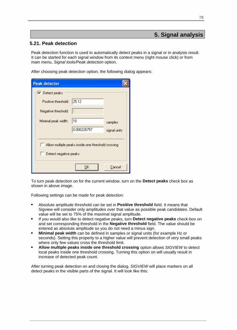
5. Signal analysis
5.21. Peak detection
Peak detection function is used to automatically detect peaks in a signal or in analysis result.It can be started for each signal window from its context menu (right mouse click) or frommain menu, Signal tools/Peak detection option.
After choosing peak detection option, the following dialog appears:
To turn peak detection on for the current window, turn on the Detect peaks check box asshown in above image.
Following settings can be made for peak detection:
Absolute amplitude threshold can be set in Positive threshold field. It means that·Sigview will consider only amplitudes over that value as possible peak candidates. Defaultvalue will be set to 75% of the maximal signal amplitude.If you would also like to detect negative peaks, turn Detect negative peaks check-box on·and set corresponding threshold in the Negative threshold field. The value should beentered as absolute amplitude so you do not need a minus sign.Minimal peak width can be defined in samples or signal units (for example Hz or·seconds). Setting this property to a higher value will prevent detection of very small peakswhere only few values cross the threshold limit.Allow multiple peaks inside one threshold crossing option allows SIGVIEW to detect·local peaks inside one threshold crossing. Turning this option on will usually result inincrease of detected peak count.
After turning peak detection on and closing the dialog, SIGVIEW will place markers on alldetect peaks in the visible parts of the signal. It will look like this:
78

5. Signal analysis
Each marker shows X-position of the peak (above) and peak amplitude (below).
By using Peak count instrument, you can automatically display or track number of peakscurrently detected in the visible signal part.
79

5. Signal analysis
5.22. Inverse FFT
Inverse FFT is a function which converts complex spectrum in a time-domain signal, i.e. thefunction which reverts FFT result back in the origin signal. To apply this function, you need toprovide complex spectrum with real and imaginary components. Applying Inverse-FFT directlyto spectrum derivate like magnitude spectrum or power spectrum is not possible becauseimportant phase information is not available anymore.
Inverse FFT in SIGVIEW is included in Signal Calculator as a binary operator. It should beapplied to a real and imaginary spectrum part as shown in the screenshot below:
The result would look like this in the Control Window:
Real and imaginary spectrum parts can be obtained in SIGVIEW in two ways:
1. Calculate FFT twice for a signal and choose "Real part" and "Imaginary part" in "Show
80

5. Signal analysis
result as" field for these two spectrums respectively. For both spectrums, windowing andzero-expand options should be turned off if you wish to get exactly the same signal afterinverse FFT. After calculating Inverse-FFT as shown above, resulting signal should be thesame (up to the calculation precision) as the origin signal. Please note that DC component ofthe origin signal will also be lost, i.e. result of the Inverse-FFT will probably be translated for aconstant offset on the Y-axis from the origin signal. To avoid it, you can use Remove DCoffset function on the origin signal before calculating its spectrum.
2. SIGVIEW distribution includes ready-to-use custom tool named "RealAndImagFFT" whichwill automatically calculate real and imaginary FFT parts in two separate windows asdescribed above. You can use it to prepare data for the Inverse-FFT function. since this tooluses no zero-padding when calculating FFTs, we recommend using power-of-2 signal lengthfor best performance.
81

5. Signal analysis
5.23. Custom filter curves
What is custom filter curve?
SIGVIEW allows you to define custom filter curves and to apply those during time-domainsignal filter or for spectrum modification. Custom filter curve is actually a sequence of[frequency, modification factor] pairs which define how should a frequency component bechanged.
For example, a band-pass filter with a pass-band between 1000 - 2000Hz could be definedthis way:
1000 0.02000 1.020000 0.0
meaning that all frequency components up to 1000Hz should be removed (factor 0.0 ), allbetween 1000Hz and 2000Hz should remain intact (factor 1.0) and all above 2000Hz up to20000Hz should be removed (factor 0.0).
Another example would be a standard a-weighting curve used in sound pressure levelmeasurement. This curve is defined in dB, i.e. signal increase or decrease dB level for certainfrequencies:
10 -70.4320 -50.3930 -40.640 -34.5450 -30.27..........
meaning that frequency components around 10Hz should be reduced for -70.43dB, around20Hz for -50.39 dB and so on...Note that we do not define upper frequency limits here as infirst examples but center frequencies of each "bin".
What is included in SIGVIEW
SIGVIEW allows you to define all those filter types manually (by editing text files) or fromexisting spectrum curves and to apply them to signals or spectrums. All filter curves used bySIGVIEW are stored in a "filters" subdirectory of the SIGVIEW data directory (usuallyC:\Documents and Settings\<UserName>\Application Data\Sigview\). For more informationabout filter file structure and creation, see bellow.
Following filter curve types are supported:
Magnitude values filter: Filter values are used as absolute magnitude values in signal units.The filter amplitude values will be subtracted from the actual signal values when filter isapplied (magnitude reduction). This means that value of 5 in a filter for certain frequency willactually reduce signal amplitude on that frequency for 5 signal units (for example Volts) whenfilter is applied. This filter will mostly be created from existing spectrum curves. For example,you can use SIGVIEW to calculate your microphone characteristic response curve, save it asa filter and subtract from a spectrum of the recorded audio.
82

5. Signal analysis
Relative dB values filter: As in second example above, this filter contains dB values tomodify certain frequency components. For example, value of -50 means that frequencycomponent will be reduced for 50dB.
Relative values filter: As described in first example above, this filter contains relativecoefficients which are used to multiply frequency components on certain frequencies (forexample 0.5 means that frequency component is reduced to 50%). This type of filter willmostly be created manually by editing filter file with editor.
Creating custom filter curves manually
Custom filter curves are stored in plain-text files with extension *.flt stored in a "filters"subdirectory of the SIGVIEW installation directory. You can create these files in any text editorand save them into "filters" directory located in SIGVIEW's application data directory (usuallyC:\Documents and Settings\<UserName>\Application Data\Sigview\). During next startup,SIGVIEW will read your file and include it in all filter functions. Each filter has 3 header lines atthe beginning and looking similar like these:
Type=DB_ADDFrequency=CENTER########10 -70.4320 -50.3930 -40.6.................
These lines are followed by rows containing frequency in Hz/value pairs using TAB (ASCII0x9) as value separator. For an example, please take a look at delivered "a-weighting.flt" file.
Type parameter (Type=) in the FLT file defines which type of filter is in the file. Followingvalues are allowed:
ABS_SUB: Corresponds to "Magnitude values filter" as described above. Following filtervalues will be interpreted as magnitude values and subtracted from corresponding signalmagnitude values.
DB_ADD: Corresponds to "Relative dB values filter" as described above. Following filtervalues will be interpreted as dB values defining how to modify certain frequency component(for example -50 means that signal magnitude on that frequency will be reduced for 50dB).
ABS_MUL : Corresponds to "Relative values filter" as described above. Following filter valueswill be interpreted as coefficients to multiply certain frequency component with (0.5 meansreduction of the magnitude for 50%).
Frequency parameter defines how to interpret frequency values. Following values for thisparameter are allowed:
CENTER: Frequency value is center frequency. Corresponding filter value will be applied toall frequencies ( (fi + fi-1)/2, (fi+fi+1)/2 ]
MAX: Frequency value is a upper limit frequency. Corresponding filter value will be applied to
83

5. Signal analysis
all frequencies ( fi-1, fi]
Creating custom filter curves from SIGVIEW
You can save any signal or analysis result from SIGVIEW as filter curve. You will usually startwith a magnitude spectrum or its averaged version. It can be directly saved as "Magnitudevalues filter". The ratio between two spectrums can, for example, be stored as "Relativevalues filter". In all cases, you will use File/Save as custom filter... main menu option on awindow containing your filter sequence. The following dialog appears after opening this menuitem:
You have to define the file name of your filter. It has to have FLT extension and it should bestored in "filters" directory under SIGVIEW's application data directory (usually C:\Documentsand Settings\<UserName>\Application Data\Sigview\). Otherwise, it will not be visible toSIGVIEW. You can also decide to store filter as a temporary file. In that case, you shouldonly give it a name - there will be no file actually stored on disk. Of course, the filter will be lostwhen you close SIGVIEW. In Filter type box you have to tell SIGVIEW what type of filter it is,
84

5. Signal analysis
i.e. how to interpret filter values later when applying the filter. These types correspond exactlyto the filter types explained above. After you press OK, filter will be saved and will beaccessible from filter and spectrum properties functions.
All filters stored in this way will use CENTER setting to interpret frequency values (seeabove).
To delete filter, simply delete its *.FLT file in filters directory.
Using custom filter curves for time-domain signal filtering
You can use custom filters to directly filter time-domain data. This feature is implemented as apart of Signal tools/Filter... menu option. After applying your filter to a time-domain signal, thedifference (or ratio) between magnitude spectrum of the original signal and magnitudespectrum of the filtered signal will correspond to the custom filter curve.
Using custom filter curves for spectrum modification
You can use custom filters to modify calculated magnitude spectrum or power spectrum justas if the filter were applied to the origin time-domain data. This option is available fromProperties dialog of any spectrum window or as general setting in Spectrum Analysis defaultsdialog. After applying your filter to a spectrum, the difference (or ratio) between originalspectrum and modified spectrum will correspond to the custom filter curve.
85

5. Signal analysis
No matter what is the type of your custom filter (dB, absolute,...), SIGVIEW will be able toapply it to all spectrum types, i.e. dB filter will be also applicable on magnitude spectrum withlinear scale values. SIGVIEW will perform all needed filter conversions internally.
For more information, see the Use custom filter curve for better measurement results section.
86
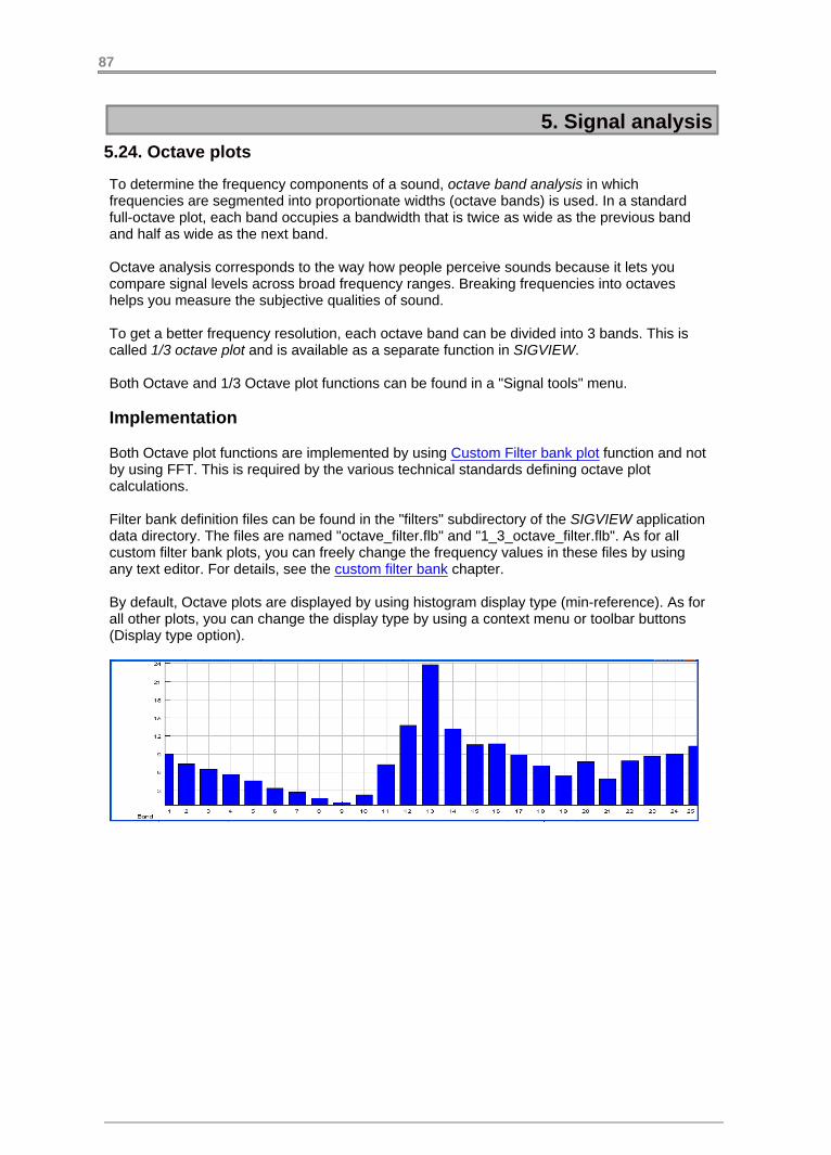
5. Signal analysis
5.24. Octave plots
To determine the frequency components of a sound, octave band analysis in whichfrequencies are segmented into proportionate widths (octave bands) is used. In a standardfull-octave plot, each band occupies a bandwidth that is twice as wide as the previous bandand half as wide as the next band.
Octave analysis corresponds to the way how people perceive sounds because it lets youcompare signal levels across broad frequency ranges. Breaking frequencies into octaveshelps you measure the subjective qualities of sound.
To get a better frequency resolution, each octave band can be divided into 3 bands. This iscalled 1/3 octave plot and is available as a separate function in SIGVIEW.
Both Octave and 1/3 Octave plot functions can be found in a "Signal tools" menu.
Implementation
Both Octave plot functions are implemented by using Custom Filter bank plot function and notby using FFT. This is required by the various technical standards defining octave plotcalculations.
Filter bank definition files can be found in the "filters" subdirectory of the SIGVIEW applicationdata directory. The files are named "octave_filter.flb" and "1_3_octave_filter.flb". As for allcustom filter bank plots, you can freely change the frequency values in these files by usingany text editor. For details, see the custom filter bank chapter.
By default, Octave plots are displayed by using histogram display type (min-reference). As forall other plots, you can change the display type by using a context menu or toolbar buttons(Display type option).
87

5. Signal analysis
5.25. Custom filter bank plot
To create different equalizer or octave plots for audio analysis, it is often needed to define abank of bandpass filters with different, possibly overlapping, frequency ranges. This task canbe performed by using "Custom filter bank" option in SIGVIEW.
Creating filter bank files
For each custom filter bank, a definition file with the extension "FLB" is created and stored inthe "filters" subdirectory of the SIGVIEW application data directory. Two example files will bestored there during SIGVIEW installation, "octave_filter.flb" and "1_3_octave_filter.flb". Thesefiles are used for Octave plots functions.
Each FLB file contains multiple rows, each representing one bandpass filter in the filter bank.For example:
14;18;A18;22.4;B22.4;28...................
First row defines a filter with bandpass from 14-18 Hz. As a label for this band in a SIGVIEWgraphics, a "A" will be shown.
Second row defines a filter with bandpass from 18-22.4 Hz. As a label for this band in aSIGVIEW graphics, a "B" will be shown.
Second row defines a filter with bandpass from 22.4-28 Hz. Since a label is not defined forthis filter, a band index, i.e. "3" will be used as label.
Each filter bank has to contain at least 4 filters in order to be used.
Settings in filter bank files
Besides frequency limits for bandpass filters, you can define some additional settings for thecalculation in the FLB file as well. All settings are added as text lines beginning with "#"character. The following settings are possible:
#X_LABEL defining label for X-axis
#Y_LABEL defining label for Y-axis
#FULL_SCALE defining the value to be considered as a "full scale" value in signal units whencalculating energy of the filtered signal in dB.
This would be an example of FLB file with settings described above:
#X_LABEL=Bands#Y_LABEL=dBFS#FULL_SCALE=3276814;18;A18;22.4;B22.4;28
88

5. Signal analysis
...................
Please note that the settings names are case sensitive.
Applying filter bank function
To apply one of defined filter bank files to a signal, use "Signal Tools/Custom filter bank..."menu option and choose the FLB file you would like to apply.
After a specific filter bank file is applied to a signal, the following procedure will performed:
1. The signal will be filtered with each filter from the filter bank2. The energy of the filtered signal (RMS) in dB (logarithmic scale) will be stored as a nextvalue in the "Custom filter bank plot".3. After all values for all filters are calculated, a plot will be shown. By default, these plots aredisplayed by using histogram display type (min-reference). As for all other plots, you canchange the display type by using a context menu or toolbar buttons (Display type option).
89

Part3D graphics
Sigview User Manual
VI

6. 3D graphics
6.1. Time FFT
Time FFT function calculates change of signal’s frequency components through time. Thesignal is divided in smaller equally spaced segments (possibly overlapped), an FFT for eachsegment is calculated and all FFT sequences are used to build a 3D graphic.
FFT calculation parameters depend on your current Spectral analysis defaults . You canchange the parameters for the calculated Time-FFT anytime by choosing Edit/Propertiesoption from the main menu or Properties from the context menu.
By choosing 3D-Tools/Time-FFT option from the main menu, you can set Time FFTparameters, calculate it and display 3D graphics.
Time FFT parameters:
91

6. 3D graphics
FFT segment length in samples: Length of a signal segment for the FFT calculation
Number of FFT segments: Number of signal segments. It can be calculated from thesegment length and offset parameters.
Offset between segments: Distance (in samples) between beginnings of consecutive signalsegments. It can be calculated from FFT segment length and the number of FFT segments.
Frequency range: Frequency range you would like to see in your graphics.
Special case of Time-FFT analysis is Spectrogram – it is the same as Time-FFT except the3D-graphics is shown from above and colored so that the amplitude differences arecolor-coded (same amplitude always has the same color). Choosing 3D tools/Spectrogramfrom the main menu brings up the same dialog as Time-FFT, except that resulting graphics isshown as Spectrogram.
Time FFT will by default not be linked to the origin signal because its calculation time can bemuch slower then real-time. If you explicitly link it to the signal, the step property of the signalwill temporarily be changed to be the same as Time FFT step property. Now, when you movethrough signal, Time-FFT will change accordingly. When you unlink Time FFT from the signal,signals step property will restore its prior value. This is done to optimize Time FFT calculation,so every time you step through signal, FFT for only one new segment will be calculated.
92

6. 3D graphics
6.2. Tracking changes as 3D graphics
It is often very important to see how the result of some analysis changes through time. If thatresult is a number, you can simply draw changes as function of one variable - time (useInstrument values log ). But, if the result is a signal, for example some FFT sequence, youcan track its changes through the time by creating a 3D graphics. Each time FFT valueschange, all its values will be added as one new column in a 3D graphics. You can perform thison FFT window but also for any other signal or analysis result window in SIGVIEW.
You can perform this function in SIGVIEW by choosing Signal tools/Track changes as 3Dgraphics option from the main menu. You will first have to determine the number of columnsin 3D graphics, i.e. how many last signal changes will be stored.
Each time signal the origin signal changes, one new column containing this new signal will beadded to 3D graphics and the ‘oldest’ column will be removed.
X-axis unit will be initially marked as ‘change’, i.e. the number of signal changes, and theY-axis units will be the same as for signal’s X-axis. After few signals are added to the 3Dgraphics, X-axis unit and range will be detected automatically by backtracking through theanalysis chain to the root signal window. If X values are equidistant (i.e. difference betweentwo consecutive values is always the same), those will be display on X-axis of the3D-graphics. If not, X-axis will switch again to a "change" unit where each new signal willsimply be labeled with its index, i.e. 0,1,2,3,4,...
If the length of origin signal changes (for example by zooming it in/out), its further changes willnot be added to the 3D graphics until you return the signal to the previous (original) length.
For more information see: Track analysis results through time as 3D graphics and Basic 3Doperations
93

6. 3D graphics
6.3. 3D graphics: basic operations and zooming
RotationIf you want to get a good look on 3D graphic from all sides, use arrow keys on your keyboardto rotate 3D graphic in all directions. This is possible only if you are not in ruler mode (seebelow).
Switching Waterfall / Mesh viewYou can switch from waterfall (lines only) to mesh (solid rectangles) view by choosing 3D
Tools/Mesh option from menu or by pressing button in toolbar. You can also use F2 keyas a shortcut to switch between views.
Ruler
By pressing TAB key or button in toolbar you can switch to ruler mode. Ruler will appearon the graphic and you will be able to move it with keyboard arrow keys. The ruler’s X,Yposition and f(X,Y) for the current ruler position will appear in status bar at the bottom of thescreen.
Zooming in/out
Zooming-in part of the graphic:
In spectrogram view, simply select the part of the graphics with mouse (rounding box), andthen choose Edit/Zoom in menu or toolbar option. If the ruler is turned on, zoom-in option willalways zoom-in to an area around the current ruler position.
Edit/Zoom out option and button from toolbar will restore the zoom positions before thelast zoom in operation.
Zoom-in graphical content of the window:
By pressing and buttons in toolbar you zoom in/out only graphical content of awindow. This zooming will affect the displaying only – the data displayed will remain the same.
Palettes: In a 3D graphics mesh mode, the color of the rectangles is defined by a currentpalette. You can define it for each window separately from its context menu or from the mainmenu. The available palettes are: Hot (red/black), Blue (blue/black), Gray (white/black),Copper (yellow/black), HSV (all colors), White (inverted gray palette)
Inverting colors: If the 3D graphics is in a Mesh mode, you can invert it colors by choosingInvert colors menu option from the context or main menu. By mot palettes, it will provide thegraphics with the light colors for the values around 0, making the graphics much moreprinter-friendly.
Z-axis adjustingWhen 3D graphic is recalculated and redrawn because its parent signal has changed, min &max values are not automatically recalculated to avoid speed loses. This can cause 3Dgraphic to go out from visible part of coordinate system, or can corrupt the color layout. If thathappens, you can select 3D Tools/Adjust Z-axis option from menu and min & max values for Zaxis will recalculate. This will solve all described problems.
94

6. 3D graphics
Exporting 3D graphics values in file: By using options File/ASCII files/Export 3D-graphics,you can export all values from the visible part of the 3D graphics in a one file. There are 3options: export in a file with X,Y,Z triples in 3 columns (tab delimited), as a matrix where firstrow contains X values, first column Y values and the rest of the file are Z values in a tabdelimited table and finally inverted variant of the second matrix format (with switched rows andcolumns). All of these file types can be loaded by, for example, MS Excel for further analysis.
Copying 3D graphics values to the clipboard: By using menu option Edit/Copy data toclipboard, all values from the visible part of 3D graphics will be copied to clipboard. The dataformat will be the same as when exporting data in ASCII: matrix where first row contains Xvalues, first column Y values and the rest of the file are Z values in a tab delimited table.
95

6. 3D graphics
6.4. Extracting signals from 3D graphics
It is often very useful to see extracted slices from 3D graphics as signals. For example, youcan extract all values at the same frequency from Time FFT, to see how that frequencycomponent changes through time.
You can perform this in SIGVIEW by selecting 3D Tools/Extract X(Y) ruler options from menu(3D graphic must be in a ruler mode). All values from the current ruler position will beextracted to a separate signal linked to this 3D graphic. By moving 3D ruler along the 3Dgraphics, this signal will redraw to show the current ruler values. Even if you turn the rulermode off, the extracted signal will keep showing the corresponding values from the 3Dgraphics (from the last ruler position).
96

6. 3D graphics
6.5. Axes settings (3D graphics)
Axes settings for 3D graphics is done through the Axes settings dialog, which appears afterselecting Edit/Axes settings option.
There are several fields in this dialog:
Max & Min fields are used for setting Z-axis range. You can enter your own values in the editbox, or you can change them by pressing up/down arrows on the right side of each edit box.
Auto button sets values in min/max fields to the actual min/max values from the graphics.
No auto scale check box: select it if you want to prevent automatic changes of the Z-axissettings when graphics values change.
Show axes check box: select it if you want to see the lines and labels of the coordinatesystem
Labels: text which appears at X, Y and Z axes if Show axes option is checked
97

6. 3D graphics
6.6. Types of 3D graphics
3D graphics are used to display any function defined by f(x,y) where x and y can be differentdomains, like frequency, time,…
There are two types of 3D graphics in SIGVIEW:
Time FFT: f(X,Y) is a function of time and frequency. The function value in some (X,Y)·point represents the intensity of the frequency component Y (Hz) in the moment X(seconds).
Tracking changes as 3D graphics : f(X,Y) depends on nature of signal that is being·logged. Y axis will be the same as X axis from that signal and X axis will represent thenumber of logged signal changes (this unit is called ‘change’).
98
6. 3D graphics
6.7. Spectrogram view
If you try to rotate 3D graphic to set viewpoint somewhere on Z axis (look 3D from above),you will find out that it is not possible. That view is implemented as a separate option calledSpectrogram view. It has been done mainly because of scrolling optimization when trackingFFT changes as 3D graphics.
You can switch to Spectrogram view by choosing 3D Tools/Spectrogram view from menu, or
pressing button in toolbar.
All operations including ruler handling, zooming, colors changing,... are the same as withstandard 3D- graphics. In addition, you can use a mouse rectangle selection to zoom-in fastto part of the spectrogram.
Spectrogram view is very useful and fast when used with 3D graphics created with “Trackchanges as 3D graphics” option, because a big part of the graphic can simply be scrolled, andonly a new data is drawn each time data in origin window (for example, FFT) changes.
Spectrogram view makes it easy to draw spectrograms in SIGVIEW.
99
6. 3D graphics
6.8. Palettes
3D graphics can use different colors to show different f(X,Y) values of represented function.One 3D graphics can use only one color set, called palette. Palette in SIGVIEW has 128colors.
You can set palette used by one 3D-graphics from its context menu or from the main menu,3D tools/Palette menu option.
Currently available palettes are:
gray·hsv·blue·pink·hot·white·jet·rainbow·winter·autumn·spring·summer·cool·
Some palettes are better used for linear scaling and some are better suited for log scales. Thebest way to see palette look & feel is to try it on an example 3D graphics.
Their definitions are in simple text files with *.pal extension (hot.pal, blue.pal, etc.). Each filehas 128 rows with 3 numeric values defining each of 128 colors as intensities of red, greenand blue (RGB). You can freely change values in these files to define your own palettes,provided that they keep same structure and number of rows.
100

PartInstruments
VII

7. Instruments
7.1. Instruments
102

7. Instruments
7.1. Instruments, overview
To calculate and monitor the changes of some numeric value, you can use SIGVIEW’sinstruments. They calculate different values from the signals or 3D graphics and display themas a number or in graphical form – as round-scale instrument.
Right-click menu on the instrument window includes many useful options: copying instrumentvalue to the clipboard, logging instrument values, editing instrument properties etc.
You can create instruments by using one of options in the Instruments and markers mainmenu section. SIGVIEW supports the following instrument types:
Marker at...: You can define X value from the signal and instrument will monitor Y value (forexample you can monitor FFT value on certain frequency)
Marker with harmonics at...: Available for FFT windows only. Shows value at desiredfrequency along with markers on all harmonics of that frequency.
103
7. Instruments
Mean: calculates mean value of the signal
Sum: calculates sum of all signal values
Const: Creates an instrument with a constant numerical value. It can be used for expressionsin the Signal calculator
RMS (Root Mean Square): If the signal include negative values, the sum instrument willprobably not be useful. In that case you can use this instrument – the square root of the meanof the squares of the signal values. RMS=sqrt((x1^2+x2^2+…..)/N).
RMS –normalized: The same as standard RMS function, but will normalize the signal first bysubtracting its mean value from all signal values.
Standard deviation: Calculates the standard deviation of the visible part of the signal.
Variance: Measure of the amount of variation within the signal values, equal to the square ofthe standard deviation.
Skewness: Measure of symmetry, or more precisely, the lack of symmetry of distribution. Adistribution, or data set, is symmetric if it looks the same to the left and right of the centerpoint. The skewness for a normal distribution is zero, and any symmetric data should have askewness near zero. Negative values for the skewness indicate data that are skewed left andpositive values for the skewness indicate data that are skewed right.
Kurtosis: Measure of whether the data are peaked or flat relative to a normal distribution.That is, data sets with high kurtosis tend to have a distinct peak near the mean, decline ratherrapidly, and have heavy tails. Data sets with low kurtosis tend to have a flat top near the meanrather than a sharp peak. A uniform distribution would be the extreme case. SIGVIEW uses"excess kurtosis" meaning that standard normal distribution has a kurtosis of zero.
Crest factor: Calculates the crest factor of the visible part of the signal.
Integral: Calculates numerical integral over the visible signal part
Weighted mean (Mean frequency): Calculates sum of products Xi * Yi divided with sum of Yi(Xi are values on x-axis and Yi corresponding values on y-axis from origin plot). If applied to aFFT plot, it is equivalent to a mean frequency.
Weighted median (Median frequency): Xi are values on x-axis and Yi corresponding valueson y-axis of the origin plot. This function calculates Xi value so that sum of Xi * Yi on bothsides of the Xi is the same (or nearly the same). If applied to a FFT plot, it is equivalent to amedian frequency.
Signal-To-Noise Ration (SNR): Calculates ratio between signal power and noise power inthe overall signal. The higher the ratio, the less obtrusive the background noise is. SinceSIGVIEW does not have any information about the real nature of your signal, it will not beable to deliver accurate values in all cases. Therefore, you should use it with pure tone signals(i.e. sine) signals to achieve best accuracy. SNR units are decibel (dB).
Total Harmonic Distorsion (THD) and Total Harmonic Distorsion + Noise (THD+N): THDis a measurement of the harmonic distortion present in the signal and is defined as the ratio ofthe sum of the powers of all harmonic components to the power of the fundamental
104
7. Instruments
frequency. Lesser THD allows the components in a loudspeaker, amplifier or microphone orother equipment to produce a more accurate reproduction by reducing harmonics added byelectronics and audio media. You should measure it in signals containing one pure tone (sine)component. THD+N means total harmonic distortion plus noise. This measurement is muchmore common and more comparable between devices. Both instrument values are calculatein decibel (dB). To convert dB values to percent values, you can use one of online calculators,for example here.
Maximum: calculates maximum value from the signal
Minimum: calculates minimum value from the signal
Maximum position: calculates the position of maximum from the signal (for examplefrequency of the max. peak in FFT)
Maximum position (interpolated): estimates the position of the maximum value moreprecisely by using interpolation. It is especially useful for determining fundamental frequencyin the spectrum with precision better then the frequency resolution of the spectrum.
Minimum position: calculates the position of minimum value from the signal
Sum 3D over frequency range: it is the only instrument applicable to 3D graphics (usuallyTime FFT). It calculates the sum of all values from the 3D graphics for one segment of the Yaxis (usually frequency).
Peak count: Shows number of peaks detected by the Peak detection function
The context menu for each signal window includes “Show 5 highest peaks” option. With thisoption turned on, SIGVIEW will show 5 markers on 5 highest signal values in the visible partof the signal.
To copy the values of all visible markers to the clipboard in a TAB-separated format, you canuse the context menu option "Copy markers to clipboard" on the signal containing themarkers.
105

7. Instruments
7.2. Instrument properties
By choosing Edit/Properties for instrument window, you will be able to set some of thefollowing instrument properties:
Type: There are 2 types of instruments:
Circle with classic round scale·Non-graphic, with numeric value only·
Modify instrument value: You can define coefficients to modify the instrument value aftercalculation. It is useful if you need a calculation slightly different than the one included inSIGVIEW , for example if the unit you would like to use needs some scaling. You can defineboth add (A) and multiply factors (B). The resulting instrument value will be calculated fromthe originally calculated value by using the following expression: NewValue = A +B*OriginalValue.
Range: Value range for instrument scale
Units: Units for instrument value (Volt, meter, etc. )
Show signal marker: This option is available only for At..., Maximum, Minimum, Maximumposition and Minimum position instruments. If you turn it on, a marker will appear in the origin
106
7. Instruments
signal, showing exact position for the value shown in instrument. You can define the contentof the marker by changing its text, or turning X/Y value display in the marker.
Critical value range: You can choose value range which represents the “red zone”. It will bemarked red on the instrument. By choosing Outside option in the radio box you will invert theselection, i.e. all values outside that range will be marked red.
Play sound on critical value: SIGVIEW will play a single beep when the value is in a criticalzone.
Execute this application on critical value: You can enter complete path of an externalapplication to be executed if the value is in a critical range, i.e. if value of the instrumententers “red-zone”. You can also define how often this application will be called. SIGVIEW willexecute defined application and pass current instrument value as a parameter to it. Forexample, if your application is “C:\MyLogger.exe”, and value of 45.4432 causes alarm to goesoff, SIGVIEW will call “C:\MyLogger.exe 45.4432”. This function can also be used to simplylog analysis values outside SIGVIEW in some regular intervals.
As an example for the external application, SIGVIEW distribution includes “Logger.exe”application. You can simply copy this file from SIGVIEW installation folder to some otherfolder and enter its path to the instrument dialog. Logger.exe will log the values passed fromSIGVIEW in a TXT file with the name SIGVIEWLog_<current date>.txt in its working directory.
Another example for such external application is ULDigital.exe, also included with SIGVIEWinstallation. This application can control digital outputs on devices compatible with UniversalLibrary from Measurement Computing(R), i.e. can turn external devices on or off. There arefollowing command line options: ULDigital.exe <duration in ms> <digital output>.where <digital output> should corresponds with UniversalLibrary's FIRSTPORTA,SECONDPORTA,... values. For example, on PMD devices these values are 10,14,18,... forchannels A0, A1, A2,... This application requires that Universal Library driver is installed.
107
7. Instruments
7.3. Logging instrument values
After you create an instrument , you can log changes of its values through time with the Loginstrument values option in Instruments and markers menu.
After you choose Log instrument values option... option from the Signal tools menu, you willhave to determine the length of the log signal (in samples). A new, empty, signal window willappear.
As soon as the instrument value changes, its new value will be added to the log window - itwill work just as old-fashioned paper tape recorder.
Scrolling and resetting
Log window will monitor all changes in the instrument and add all consecutive values frominstrument into one signal. When this signal reaches maximum length you determined, thedisplay will start to scroll, removing oldest values and adding new ones. By choosing Resetdata from the Log window’s context menu (or pressing F3), you can clear all value and startlogging again. By using Start/Stop options from the context menu, you can stop logging andstart it again.
X-axis units
Value log signal will try to determine values for its X-axis automatically by backtrackingthrough the analysis chain to the root signal window. If those X values are equidistant (i.e.difference between two consecutive values is always the same), those will be display onX-axis of the instrument log. If not, X-axis will switch to unit called "change" where each newvalue will simply be labeled with its index, i.e. 0,1,2,3,4,...
Long-time logging of instrument values in a file
Since instrument log keeps its data in your computer's RAM, total storage length is verylimited. For long-time recording of signal values, you can use Logging data to file optionconnected to a log instrument window. For example, this would be a Control Window displayof a system to store max. frequency from an FFT into a file.
Instrument log in this system stores only a last 100 values and can be used for monitoring.File log window, on the other hand, stores all values which are added to a instrument log intoa file.
For more information, see Track changes of signal parameters through time How-To section.
108

7. Instruments
7.4. Instruments statistics
Each instrument includes statistics functions which automatically track its maximal, minimaland average values.
To see one of these automatically calculated statistical values, you can use instrument'scontext menu:
As a default setting, each instrument will show its current value, i.e. "Show as CURRENTinstrument value" option will be selected.
After choosing some of statistical values (AVERAGE, MINIMAL, MAXIMAL), the instrumentwill switch to displaying the chosen statistic value. That will be indicated by "AVG", "MIN" or"MAX" prefix to the instrument value.
By choosing "Reset statistical values" options from the context menu, you will reset allstatistical values to the current value of the instrument.
After switching instrument display to some of statistical values, it will affect all windowsattached to the instrument window as well, for example instrument value log.
109
PartData acquisition
Sigview User Manual
VIII

8. Data acquisition
8.1. Data acquisition overview
SIGVIEW supports real-time data acquisition from the following device types:
Windows compatible sound cards (up to 16-bit resolution, up to 2 channels, old-style·drivers)
DirectSound compatible sound cards ( maximal supported sound card resolution,·typically 24-bit for professional sound cards, typically all available channels)
ASIO sound card drivers (by Steinberg) for low-latency and high fidelity sound card·recording
National Instruments(R) DAQ cards with support for NiDAQmx drivers (see·www.ni.com)
National Instruments(R) DAQ cards with support for NiDAQ drivers (see www.ni.com)·
Measurement Computing(R) DAQ cards supported by Universal Library (see·www.measurementcomputing.com)
Data acquisition simulation by reading data from specially prepared signal file·
SIGVIEW offers a generic user interface and settings for data acquisition from all supporteddevices. Device-specific settings (if any) are available through additional dialogs. To start dataacquisition, choose Data acquisition/Open data acquisition menu option. A dialog appearswhich allows you to choose data acquisition device and to change the data acquisitionsettings:
111
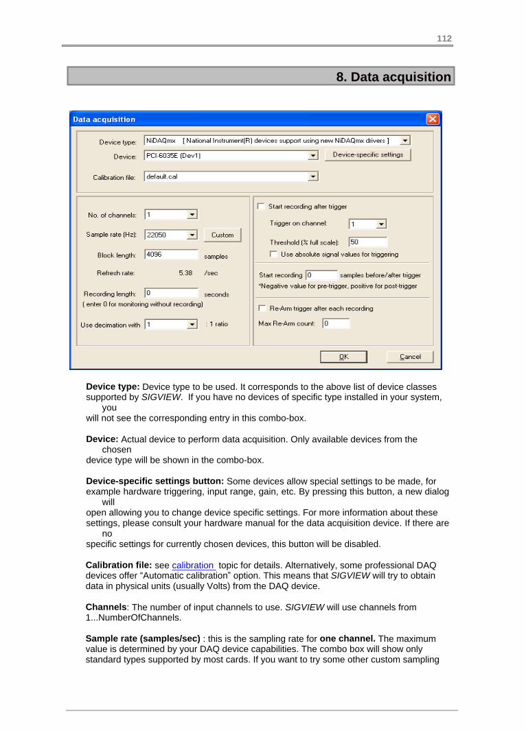
8. Data acquisition
Device type: Device type to be used. It corresponds to the above list of device classessupported by SIGVIEW. If you have no devices of specific type installed in your system,
youwill not see the corresponding entry in this combo-box.
Device: Actual device to perform data acquisition. Only available devices from thechosen
device type will be shown in the combo-box.
Device-specific settings button: Some devices allow special settings to be made, forexample hardware triggering, input range, gain, etc. By pressing this button, a new dialog
willopen allowing you to change device specific settings. For more information about thesesettings, please consult your hardware manual for the data acquisition device. If there are
nospecific settings for currently chosen devices, this button will be disabled.
Calibration file: see calibration topic for details. Alternatively, some professional DAQdevices offer “Automatic calibration” option. This means that SIGVIEW will try to obtaindata in physical units (usually Volts) from the DAQ device.
Channels: The number of input channels to use. SIGVIEW will use channels from1...NumberOfChannels.
Sample rate (samples/sec) : this is the sampling rate for one channel. The maximumvalue is determined by your DAQ device capabilities. The combo box will show onlystandard types supported by most cards. If you want to try some other custom sampling
112

8. Data acquisition
rate, press “Custom” button and enter the sample rate manually. Please note that somesound cards will simply report that they support any sample rate even if they don’t supportit in hardware. Those will simply try to simulate it on a driver level. If you want to avoid it,please consult the card's manual to determine which sample rates are really supported.Most devices do not allow all possible sample rate settings. SIGVIEW will try to find thenext possible sample rate settings applicable to your device and apply it automatically.You will see the actual sampling rate in the status bar of the data acquisition window afteryou close this dialog.
Block length (samples): determines how much samples will be shown in a windowduring acquisition.
Recording length (sec): If you want only to monitor the signal without any saving chooselength of zero. In that case, you will always have only the last "Block length" samplesavailable in your data acquisition window. Otherwise, enter the duration in seconds youwant to save. During acquisition, you will always see the last "Block length" samples inyour acquisition window but you will see all samples after zooming-out. Please note thatSIGVIEW stores all data in physical memory (RAM). Therefore, saving more then severalminutes of data by using this method is not recommended. You can use Logging data tofile feature for that purpose.
Decimation ratio: To reduce the amount data which has to be processed during analysis,you can use decimation feature, i.e. convert multiple samples from the DAQ device to onesample in SIGVIEW. You can define a decimation ratio by determining how manysamples from the DAQ device will be converted to one sample in SIGVIEW. If you choosedecimation ratio greater then 1, SIGVIEW will calculate the actual sample rate and show itas a read-only information under this field. For example, if the sample rate on Sound cardis 44100Hz, and a decimation ratio is 100, then the actual sample rate in SIGVIEW will be441Hz.
Start recording after trigger: If you check this option, recording will not start immediatelyafter pressing START button – SIGVIEW will wait for a specific trigger (i.e. signal level)value in the signal and then start recording automatically. Trigger behavior and thedefinition of trigger value is determined by using the following options:
Trigger on channel: Determines which of the data acquisition channels willSIGVIEW monitor for a trigger value. It is possible to receive data on one channeland use the other one only for triggering.
Threshold (% full scale): This option determines which signal level is exactlyregarded as a trigger value in the signal. Each sample with the amplitude higher thanthe threshold, by default 50%, from the maximum possible signal amplitude will beregarded as a trigger. For example, if your trigger is very strong signal impulse, youcan set threshold to 90%. If you would like to use absolute signal values for triggering,select "Use absolute signal values for triggering" option. In that case, negativesignal values will also be taken into account as trigger.
Start recording X samples before/after the trigger: This option determines onwhich position, relative to the trigger appearance, will SIGVIEW start recording. Theposition is defined in number of samples. Negative value will cause SIGVIEW to startrecording before the trigger and positive value after the trigger. Maximal number ofsamples you can set for pre-trigger option is equal to "Block length" setting (seeabove).
113

8. Data acquisition
Re-Arm trigger trigger after each recording: After data acquisition is started aftertrigger and required signal length has been recorded, data acquisition would normallystop. By turning this option on, you can instruct SIGVIEW to automatically start newdata acquisition window after the triggered data acquisition has been finished. Newdata acquisition window will use exactly the same settings as the previous one, i.e.will wait on trigger, record, and then start new data acquisition window. This way, youcan let SIGVIEW automatically record multiple triggered signal events. Eachrecording will be stored in a separate window. To limit numbers of new windowswhich can be created during this operation, you can set "Max Re-Arm Count" option.Please note that trigger Re-Arm options make sense only if you define some specificrecording length. If you use the value of zero (monitoring only), trigger will never bere-armed because recording will never stop.
For further information about the triggering, please see the How-To:Using data acquisition triggering options
After you set all these data acquisition parameters and press OK button, one or more signal
windows will appear (depending on number of channels). Now you can press button ontoolbar or choose Data acquisition/Start menu option to start data acquisition. If you choose
acquisition length of 0 (monitoring only), you can stop it by pressing button on the toolbaror choosing Data acquisition/Stop menu option. Otherwise, data acquisition will stopautomatically after the desired acquisition length is reached. While data acquisition is running,you can work with the signal window as you would with any window containing static signal:for example, you can perform FFT of running signal, track its changes as 3D graphics, andyou will have real 3D spectrum analyzer.
After data acquisition has finished, the signals in data acquisition signal windows arezoomed-in to show only the last recorded block. You will have to choose Zoom-out option tosee the whole recorded signal.
If you choose ‘File’ driver type you will be able to simulate data acquisition by reading datafrom file in 16-bit signed binary format (You can store any data in that format by using Binaryfile export feature). After clicking on “Device specific options” button you will be able to choosethe file name. SIGVIEW will try too keep the desired sample rate if there is enough data in thefile.
114

8. Data acquisition
8.2. Calibration
Signal data received from the A/D device is for SIGVIEW only a series of samples withdifferent numeric values. For example, each sample from the sound card has usually a valuebetween -32767 and 32767 (16-bit resolution). Of course, these values have no physicalmeaning. To transfer these values into meaningful physical values like Volt, meter, Celsius,etc., you have to tell SIGVIEW how to convert generic numeric values into real word units.This complete transformation is described in a ‘calibration file’. You can create as manycalibration files you want, and use them for different data acquisitions.
By choosing Data acquisition/Sound card calibration option from the main menu, you will opena calibration dialog where you can create a calibration file through 6 simple steps:
Use Data acquisition menu option to record constant signal with known amplitude1.(for example 5V) from your DAQ device. Use only "default.cal" calibration file forthis step.Measure the average value of the signal recorded by SIGVIEW during first step2.and enter it in ‘Recorded input level’ field.Enter the actual amplitude level in physical units which corresponds to the signal3.recorded during first step in ‘Input level in physical units’ field. You can alsodefine if this value should be considered as peak or RMS value.Enter the description of your physical units (for example V or Volt) in field4.‘Physical unit used’.You can also define offset to be added to recorded values (in physical units).5.Save your calibration file and use it later for data acquisition in Data acquisition6.dialog.
115

8. Data acquisition
All calibration files should be saved in the “Calibration” folder located in the SIGVIEW'sapplication data directory (usually C:\Documents and Settings\<UserName>\ApplicationData\Sigview\). Each of these calibration files can be used later for data acquisition.There is one special data acquisition file, “default.cal”, which is distributed with SIGVIEW andused by default. It leaves recorded data from the DAQ device just as they are, without anyconversion. You should not change the content of this file.
116

8. Data acquisition
8.3. Logging data to file
Accessible through menu option Signal tools/Log data in file or Data acquisition/Log data infile
Data acquisition operations can produce a large amounts of signal data which can not bestored in RAM. This function can be used in such cases to store all signal data from one dataacquisition window in files on the hard-disk.
Also, you can use this function for a long-time instrument values logging to a file. See Logginginstrument values for details.
After choosing this menu option, following dialog appears:
Target folder: Type or choose directory where signals should be stored. The directory shouldalready exist.
File name prefix: To make file names recognizable, you can define prefix string which will beadded to the beginning of each created file name.
Create new file when file size of …MB has been reached: You can limit the size of singlefiles. After reaching length you defined here, SIGVIEW will create new file and continuestoring data in it. If you set maximal file size to 0, SIGVIEW will create new file for each newblock from the origin window.
Wait for manual “Start” command: If you turn this option on, log window will not startstoring data after it has been created, but will rather wait on your command. You canmanually start and stop logging process by using context menu (right mouse button) options
117

8. Data acquisition
on the logging window.
After you set all properties for signal logging and press OK button on this dialog, log windowwill appear:
It shows all information about the logging process including current file, amount of storeddata, number of files and average data rate.
Signal files will be created in target folder and named<prefix>_<YYYYMMDD>_<HHMMSS>.SIG.To make data storage fast enough, data is stored in a 32-bit binary float format without anyheader information. File extension will always be “*.SIG”. All additional data like sampling rateor start time is stored in a TXT file having the same name as stored SIG file.
To load SIG files in SIGVIEW, please use File/Open data log file…. This function will load SIGfile and automatically read its additional information from TXT file. You can store your signal inWAV or any other supported format afterwards.
118
PartCommand-linefunctionality
IX

9. Command-line functionality
9.1. Concept
SIGVIEW supports various command-line parameters enabling you to use some of SIGVIEWfunctions from external applications or batch files. Since this feature is based on simplecommand-line invocation, it can be used from any other programming language orenvironment capable of calling other applications.
Typical application examples for command-line invocation would be to perform the sameanalysis on many different files or to perform some live signal analysis according to a timeschedule.
General syntax of command-line invocation is of the form:
Sigview32.exe <action> <parameters>
Each command invocation checks if there is already SIGVIEW instance running and if yes,sends command to it. Otherwise, new SIGVIEW instance is started and executes thecommand. To make calling Sigview32.exe easier, you can use environment variableSIGVIEW_EXE which contains full path of the SIGVIEW executable. For example, in a batchfile it would look like this:
%SIGVIEW_EXE% <action> <parameters>
Instead of providing single function for each analysis feature in SIGVIEW, command-lineinterface is based on creating and reusing Sigview WorkSpace files (SWS). This means thatyou will always create a workspace file first, containing the basics of analysis you would like tocontrol remotely. For more details about creating and using SWS files, please proceed here.First command you will use will probably be loading of SWS file, for example:
%SIGVIEW_EXE% -loadsws c:\myworkspace.sws
After the SWS has been loaded, you will be able use various commands to start/stopanalysis, save data to a file etc. For example, to save content of a window to a 16-bit WAVfile, you would use:
%SIGVIEW_EXE% -savewav16 window1 "c:\my dir\file1.wav"
To be able to reference single windows from your workspace, as "window1" in aboveexample, you have to assign those a name before saving your SWS file. It is done by using"Edit/Change Window title" menu option. Instead of default window name, assign window aname which describes well its usage and can be used in command line calls, for example"daq_window", "myfft1" or "result".
For detailed information about command-line invocation, please see Reference and Exampleschapters.
120

9. Command-line functionality
9.2. Command reference
This chapter lists all command-line actions and parameters you can use with SIGVIEW, aswell as some general rules for using them.
1. General rules valid for all command-line actions:
You should always use SIGVIEW_EXE environment variable instead of actual SIGVIEW·executable file name, for example: %SIGVIEW_EXE% -loadswsc:\myworkspace.sws. This will make it easier to reuse your scripts on anothercomputer or if your SIGVIEW installation changes. This environment variable will bedefined automatically during SIGVIEW installation.For all references to a <windowname>, you have to use the window's name as visible in·its title bar. Usually, you will use "Edit/Change window title" menu option to give a simplename to a window before saving a Workspace or a Tool file.Any command parameter which includes spaces, for example "my window" or c:\Program·files\myfile.wav" has to be enclosed in quotes (general rule for Windows command linecalls)All file paths are full paths including directory and file name, for example "c:\my dir\my·file.txt"You should use only one command in each call. To execute multiple commends, use·multiple SIGVIEW calls (multiple lines in the batch file).
2. Full list of command-line actions and options:
%SIGVIEW_EXE% -loadsws <sws_file_name> [<signalfilename> ...]Loads Workspace file in SIGVIEW. If workspace has been saved without absolute file namesin it, you can define those as additional parameters (full file names) in order of theirappearance in workspace file. See Loading and saving workspaces for more information.
%SIGVIEW_EXE% -hideHides SIGVIEW window
%SIGVIEW_EXE% -showShows SIGVIEW window again if it was hidden with the -hide command
%SIGVIEW_EXE% -closeallCloses all opened windows
%SIGVIEW_EXE% -daqstart <windowname>Starts data acquisition of a window with the specified name. Of course, window must be Dataacquisition window. The effect will be the same as if choosing "Data acquisition/Start dataacquisition" main-menu option. If you would like to start multichannel data acquisition, it isenough to call this command for the first channel.
%SIGVIEW_EXE% -daqstop <windowname>Stops data acquisition of a window with the specified name. Of course, window must be Dataacquisition window. The effect will be the same as if choosing "Data acquisition/Start dataacquisition" main-menu option. If you would like to stop multichannel data acquisition, it isenough to call this command for the first channel.
121

9. Command-line functionality
%SIGVIEW_EXE% -playnotone <windowname>Plays signal in a specified window without tone output. The effect will be the same as ifchoosing "Play&Navigate/Play (no sound)" main-menu option.
%SIGVIEW_EXE% -playwithtone <windowname>Plays signal in a specified window with tone output. The effect will be the same as if choosing"Play&Navigate/Play signal(with sound)" main-menu option.
%SIGVIEW_EXE% -playstop <windowname>Stops signal playing in a specified window started with -playnotone or -playwithtone options.The effect will be the same as if choosing "Play&Navigate/Stop playing" main-menu option.
%SIGVIEW_EXE% -zoomout <windowname>Zoom-out signal in a specified window so that the whole signal is visible. It should always beused before storing signal in a file if you would like to save the whole signal. Otherwise, only avisible signal part will be stored.
%SIGVIEW_EXE% -zoomin <windowname> <length_in_samples>[<offsett_in_signal_units>]Zoom-in signal in a specified window to the specified length (in samples) starting from someoffset (in signal units, for example seconds). If offset is omitted, signal beginning will be used.For example, %SIGVIEW_EXE% win1 256 0.6 will zoom-in signal in window "win1" to 256samples starting from 0.6s.
%SIGVIEW_EXE% -savewav16 <windowname> <full_file_name>Saves visible part of the signal in specified window to a 16-bit WAV file. If you would like tosave the whole signal in a file, perform -zoomout command first (see above). For example,"%SIGVIEW_EXE% -savewav16 sig_win_1 c:\MyFiles\test.wav".
%SIGVIEW_EXE% -savewav32 <windowname>Saves visible part of the signal in specified window to a 32-bit WAV file (32-bit float format). Ifyou would like to save the whole signal in a file, perform -zoomout command first (see above).For example, "%SIGVIEW_EXE% -savewav32 sig_win_1 c:\MyFiles\test.wav".
%SIGVIEW_EXE% -saveascii <windowname>Saves visible part of the signal in specified window to ASCII file format. ASCII file will containtwo columns: one with X values and one with Y values from the signals. If you would like tosave the whole signal in a file, perform -zoomout command first (see above). For example,"%SIGVIEW_EXE% -saveascii sig_win_1 c:\MyFiles\test.wav".
%SIGVIEW_EXE% -savebitmap <windowname> <bitmap_filename>Saves graphical content of the <windowname> window as BITMAP file (*.bmp). This will workonly if main SIGVIEW window is currently visible.
%SIGVIEW_EXE% -getvalue <windowname>Gets current value from an instrument window with specified window name. Instrument valuewill be converted in text format, for example "4.325" and forwarded to the standard output.You can use standard batch file syntax to forward that value to a file or to another application.For example, "%SIGVIEW_EXE% -getvalue instr_max >> myinstrlog.txt" or
122

9. Command-line functionality
"%SIGVIEW_EXE% -getvalue instr_max | myinstrprocessor.exe".
%SIGVIEW_EXE% -repeatforever on|offTurns"Repeat forever" play option "on" or "off". This is a global setting valid for all windows.
%SIGVIEW_EXE% -playfast on|offTurns "Play as fast as possible" play option "on" or "off". This is a global setting valid for allwindows.
%SIGVIEW_EXE% -autovolume on|offTurns "Adjust volume automatically" play option "on" or "off". This is a global setting valid forall windows.
%SIGVIEW_EXE% -closeappCloses SIGVIEW.
%SIGVIEW_EXE% -waitms <number_of_ms_to_wait>Waits specified number of milliseconds and returns. It is useful as pause command if yourprogramming language does not support it directly, for example when using batch files.Please note that time resolution of this command is very coarse - you should expect jitter ofup to 100ms.
%SIGVIEW_EXE% -helpShows list of supported commands in a message box.
For further information about using this commands, see Examples section.
123

9. Command-line functionality
9.3. Examples
This chapter contains several examples for using command-line parameters in SIGVIEW. Allexamples are implemented as MS Windows batch files. You can find the source code of theseexamples in "Scripts" subdirectory of the SIGVIEW installation directory:
1. Record 10 seconds of signal and save signal to a file along with itsaveraged spectrum
In this example, we will create a batch file which starts 10 seconds of data acquisition, savesresulting signal in a file along with its average spectrum.
You should create a Workspace containing data acquisition window (from any device), FFT ofdata acquisition window and Averager of the FFT window. Control window display should looklike this:
Data acquisition window has to have defined acquisition length (10s). You should renamedata acquisition window to "daq_window" and Averager window in "average_window". Savethis workspace in, for example, c:\test\daq_average.sws.
The following batch script will use this workspace to perform 10 seconds of acquisition andsave recorded signal and average spectrum at the end.
REM close any opened windows%SIGVIEW_EXE% -closeall
REM load workspace%SIGVIEW_EXE% -loadsws c:\test\daq_average.sws
REM start data acquisition%SIGVIEW_EXE% -daqstart daq_window
REM wait 11 seconds - until we are sure that acquisition is finished%SIGVIEW_EXE% -waitms 11000
REM stop data acquisition%SIGVIEW_EXE% -daqstop daq_window
REM save average spectrum%SIGVIEW_EXE% -saveascii average_window c:\test\average_fft.dat
REM zoom-out data acquisition window and save it to WAV file%SIGVIEW_EXE% -zoomout daq_window%SIGVIEW_EXE% -savewav32 daq_window c:\test\daq_signal.wav
REM close SIGVIEW%SIGVIEW_EXE% -closeapp
124
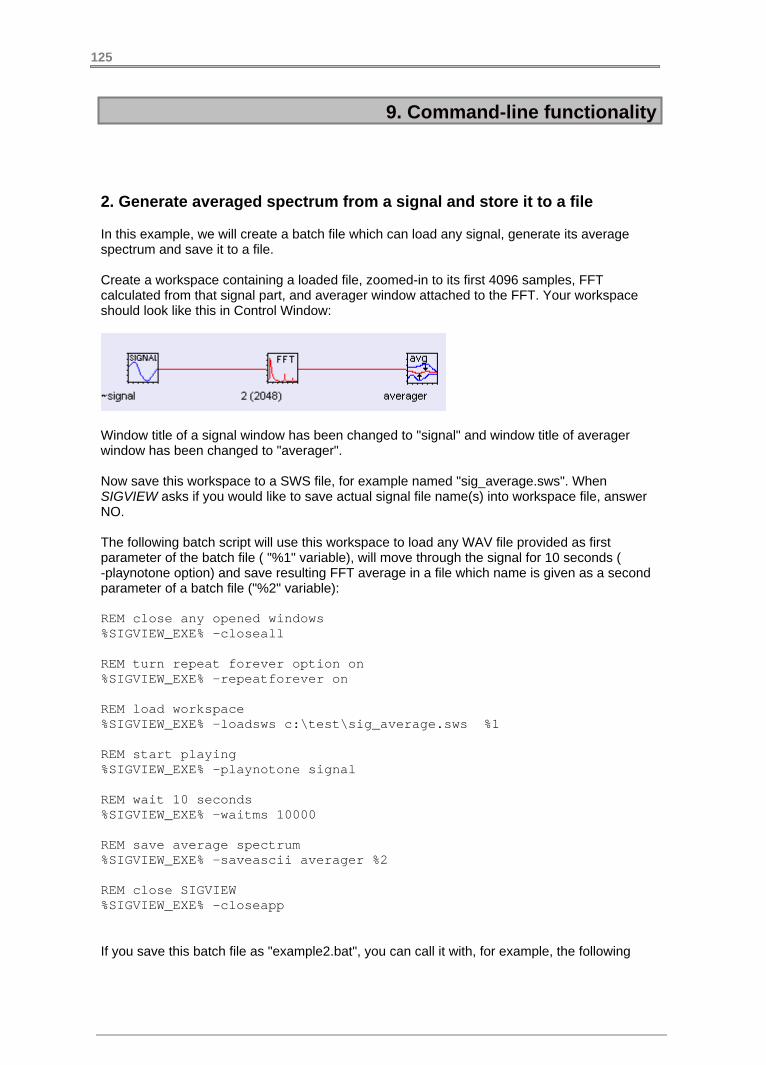
9. Command-line functionality
2. Generate averaged spectrum from a signal and store it to a file
In this example, we will create a batch file which can load any signal, generate its averagespectrum and save it to a file.
Create a workspace containing a loaded file, zoomed-in to its first 4096 samples, FFTcalculated from that signal part, and averager window attached to the FFT. Your workspaceshould look like this in Control Window:
Window title of a signal window has been changed to "signal" and window title of averagerwindow has been changed to "averager".
Now save this workspace to a SWS file, for example named "sig_average.sws". WhenSIGVIEW asks if you would like to save actual signal file name(s) into workspace file, answerNO.
The following batch script will use this workspace to load any WAV file provided as firstparameter of the batch file ( "%1" variable), will move through the signal for 10 seconds (-playnotone option) and save resulting FFT average in a file which name is given as a secondparameter of a batch file ("%2" variable):
REM close any opened windows%SIGVIEW_EXE% -closeall
REM turn repeat forever option on%SIGVIEW_EXE% -repeatforever on
REM load workspace%SIGVIEW_EXE% -loadsws c:\test\sig_average.sws %1
REM start playing%SIGVIEW_EXE% -playnotone signal
REM wait 10 seconds%SIGVIEW_EXE% -waitms 10000
REM save average spectrum%SIGVIEW_EXE% -saveascii averager %2
REM close SIGVIEW%SIGVIEW_EXE% -closeapp
If you save this batch file as "example2.bat", you can call it with, for example, the following
125

9. Command-line functionality
command line:
example2.bat c:\test\mysignal.wav c:\test\average_fft.dat
3. Start data acquisition and log signal RMS energy in file each second
In this example, we will create an endless instrument logger. It will start data acquisition,calculate continuously RMS of the current signal, and save it to a file along with the systemtime.
Create a workspace containing data acquisition window (acquisition length = 0, any device)and an RMS instrument. Your workspace should look like this in Control Window:
Window title of a signal window has been changed to "daq_window" and window title of RMSinstrument window has been changed to "rms_window".
This would be the content of a batch file:
REM close any opened windows%SIGVIEW_EXE% -closeall
REM load workspace%SIGVIEW_EXE% -loadsws c:\test\daq_rms.sws
REM start data acquisition%SIGVIEW_EXE% -daqstart daq_window
REM endless loop:start
REM wait 1 second%SIGVIEW_EXE% -waitms 1000
REM read value from rms_window and add it to text file%SIGVIEW_EXE% -getvalue rms_window >> c:\test\values.txt
REM time information after the valueecho %time% >> c:\test\values.txt
REM loop againGOTO start
Since this is an endless loop, you will have to stop the batch file manually. The result file willlook like this:
0.011391 20:34:30,35
126

PartRegistration
X

10. Registration
10.1. Registration: How?
All SIGVIEW licenses cover the Windows 95/98/NT/2000/XP/Vista/win7
Procedure for ordering SIGVIEW:
Online ordering
Visit http://www.sigview.com/order.htm for further info about pricing and ordering options
or go directly to the order page:
https://secure.element5.com/register.html?productid=133912
to order SIGVIEW online and secure.
All major credit cards are accepted. Wire transfer or check payments are also available.
What will happen after you order Sigview license?
You will receive an e-mail containing your registration data assembled from combination ofyour user name, e-mail address and registration key. You should enter these values in theregistration dialog (Help/Registration… in menu) and restart SIGVIEW once. If yourregistration was successful, your registration data will be shown in SIGVIEW About box(Help/About… in menu).
If your trial period is already expired you will be able to enter registration dialog immediatelyafter starting SIGVIEW, before “Trial expired…” message.
If you have any problems or need additional info please send an e-mail to [email protected] .
128

10. Registration
10.2. Registration: Why?
SIGVIEW is not a free software. You are hereby licensed to use SIGVIEW for evaluationpurposes without charge for a period of 21 days. If you want to use it after the 21 dayevaluation period, a registration fee is required. For detailed info, please visithttp://www.sigview.com
Why should you do it?
1. You will get your registration key, which enables you to use your copy of SIGVIEW after21-day evaluation period (it will also remove that boring license dialog that appears each timeyou start SIGVIEW)
2. You will get all later minor updates completely free, with huge discount on all new majorversions or new products
3. You will get a chance to order SIGVIEW improvements or customization
129

PartHow-To
Sigview User Manual
XI

11. How-To
11.1. Use custom filter curve for better measurement results
Measurement and data acquisition devices like microphones or sound cards have their ownfrequency characteristics which is added to your signal during recording, i.e. corrupts yoursignal. By using Custom Filter curve SIGVIEW feature, you can measure these effects andremove them automatically from recorded signals.
1. Let us take sound card device as an example and try to measure its frequency responsefirst. Before you start, you should disconnect all sound input devices like microphones - wewant to measure only internal sound card frequency characteristics in this example. Open"Data acquisition" dialog ("Data Acquisition/Open data acquisition" menu item), chooseDirectSound as device type and your sound card name as "Device". Leave all other defaultsettings. Press OK and data acquisition signal window will open.
2. While on data acquisition signal window, press FFT button in toolbar to calculate spectrumof a signal and then choose "Signal tools/Averager" option on spectrum window. Openproperties of the FFT window (Properties option in Context-Menu) and turn off "ApplyWindow" option. The result in Control Window should look like this:
3. Now go to data acquisition signal window and choose "Data acquisition/Start" menu option(or REC) button in toolbar. Recording from the sound card will start, signal and spectrum will
131
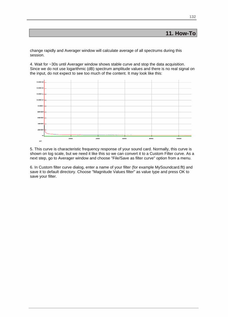
11. How-To
change rapidly and Averager window will calculate average of all spectrums during thissession.
4. Wait for ~30s until Averager window shows stable curve and stop the data acquisition.Since we do not use logarithmic (dB) spectrum amplitude values and there is no real signal onthe input, do not expect to see too much of the content. It may look like this:
5. This curve is characteristic frequency response of your sound card. Normally, this curve isshown on log scale, but we need it like this so we can convert it to a Custom Filter curve. As anext step, go to Averager window and choose "File/Save as filter curve" option from a menu.
6. In Custom filter curve dialog, enter a name of your filter (for example MySoundcard.flt) andsave it to default directory. Choose "Magnitude Values filter" as value type and press OK tosave your filter.
132

11. How-To
7. You can use this saved filter for any data analysis using sound card signal to correct yourmeasurement and remove artifacts caused by the sound card imperfection. To do so, go toyour data acquisition signal from step 1 and apply "Signal tools/Filter..." menu option on it. Inthe dialog, choose your saved MySoundcard.flt filter. It means that we remove from the signalexactly the frequency components introduced by the sound card:
133
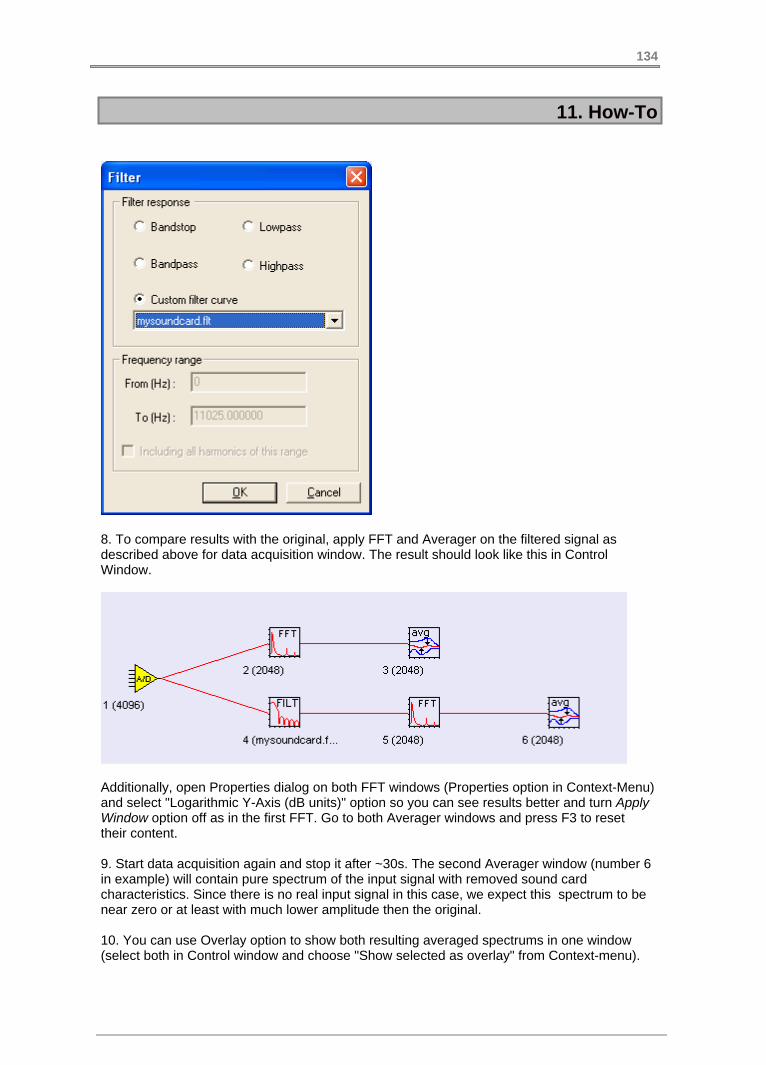
11. How-To
8. To compare results with the original, apply FFT and Averager on the filtered signal asdescribed above for data acquisition window. The result should look like this in ControlWindow.
Additionally, open Properties dialog on both FFT windows (Properties option in Context-Menu)and select "Logarithmic Y-Axis (dB units)" option so you can see results better and turn ApplyWindow option off as in the first FFT. Go to both Averager windows and press F3 to resettheir content.
9. Start data acquisition again and stop it after ~30s. The second Averager window (number 6in example) will contain pure spectrum of the input signal with removed sound cardcharacteristics. Since there is no real input signal in this case, we expect this spectrum to benear zero or at least with much lower amplitude then the original.
10. You can use Overlay option to show both resulting averaged spectrums in one window(select both in Control window and choose "Show selected as overlay" from Context-menu).
134

11. How-To
The result will be a window showing both average spectrums. The red one is original and ablack one is filtered. Obviously we achieved to reduce sound card noise for ~130 dB by usingcustom filter curve. The result is almost perfectly flat curve as close to zero as it getsconsidering our calculation precision.
11. You can use this method to calculate frequency characteristics of any other more complexdata acquisition system including microphones, sensors etc.
12. Another method to use Custom filter curve is to apply it to a spectrum instead of using itas signal filter. In that case, you see how the spectrum would look like if you would applycustom filter curve as a filter on a signal.
135

11. How-To
11.2. Track changes of signal parameters through time
We will show you here how to track changes of some signal parameters during dataacquisition or monitoring.
1. Let us take sound card device as an example. You can connect some signal source to itbefore you start (microphone). Open "Data acquisition" dialog ("Data Acquisition/Open dataacquisition" menu item), choose DirectSound as device type and your sound card name as"Device". Leave all other default settings. Press OK and data acquisition signal window willopen.
2. While on data acquisition signal window, press FFT button in toolbar to calculate spectrumof a signal. Spectrum window appears and Control Window should look like this:
3. As an example, we will track changes in signal RMS energy and the position of the peakspectrum frequency. Click on signal acquisition window and select "Instruments andmarkers/RMS" main menu option. Then click on FFT window and select "Instruments andmarkers/Maximum position (with marker)" main menu option. Two instrument windows appearshowing current values from the signal and spectrum (all zeros because data acquisition isnot running yet) The resulting Control Window should look like this:
136

11. How-To
4. Now we would like to track (log) instrument values as they change through time. To do thisclick on each of two instrument windows and select "Log instrument values" from theirright-click menu. In the small dialog asking you about buffer length for a log, leave defaultvalue of 100. Control window should look like this:
5. Now go to data acquisition signal window and choose "Data acquisition/Start" menu option(or REC) button in toolbar. Recording from the sound card will start and instruments willchange their values. On each instrument value change, the last value will be stored in acorresponding log window - log window signal will grow as new values come.
6. Note that X-axis units on log window is "change" - it is simply an index of a value changestarting from 0.
7. After 100 changes (remember your setting for buffer length), log windows will be full and
137

11. How-To
display will start scrolling. You can use context menu to reset data (i.e. start from thebeginning) or to stop/start logging. Value log signal will try to determine values for its X-axisautomatically by backtracking through the analysis chain. If those X values are equidistant(i.e. difference between two consecutive values is always the same), those will be display onX-axis. If not, X-axis will switch to unit called "change" where each new value will simply belabeled with its index, i.e. 0,1,2,3,4,...
8. Instrument log windows can be used as any other signal window, i.e. you can calculate itsspectrum, show them in overlay with other signals, store values in ASCII file etc.
138
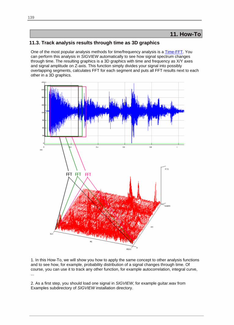
11. How-To
11.3. Track analysis results through time as 3D graphics
One of the most popular analysis methods for time/frequency analysis is a Time-FFT. Youcan perform this analysis in SIGVIEW automatically to see how signal spectrum changesthrough time. The resulting graphics is a 3D graphics with time and frequency as X/Y axesand signal amplitude on Z-axis. This function simply divides your signal into possiblyoverlapping segments, calculates FFT for each segment and puts all FFT results next to eachother in a 3D graphics.
1. In this How-To, we will show you how to apply the same concept to other analysis functionsand to see how, for example, probability distribution of a signal changes through time. Ofcourse, you can use it to track any other function, for example autocorrelation, integral curve,...
2. As a first step, you should load one signal in SIGVIEW, for example guitar.wav fromExamples subdirectory of SIGVIEW installation directory.
139
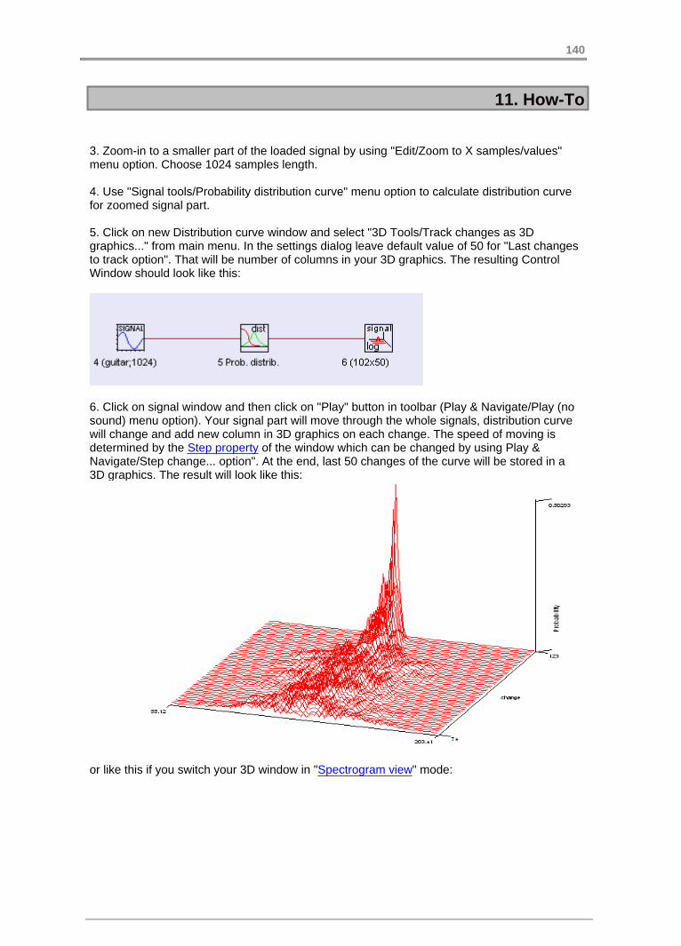
11. How-To
3. Zoom-in to a smaller part of the loaded signal by using "Edit/Zoom to X samples/values"menu option. Choose 1024 samples length.
4. Use "Signal tools/Probability distribution curve" menu option to calculate distribution curvefor zoomed signal part.
5. Click on new Distribution curve window and select "3D Tools/Track changes as 3Dgraphics..." from main menu. In the settings dialog leave default value of 50 for "Last changesto track option". That will be number of columns in your 3D graphics. The resulting ControlWindow should look like this:
6. Click on signal window and then click on "Play" button in toolbar (Play & Navigate/Play (nosound) menu option). Your signal part will move through the whole signals, distribution curvewill change and add new column in 3D graphics on each change. The speed of moving isdetermined by the Step property of the window which can be changed by using Play &Navigate/Step change... option". At the end, last 50 changes of the curve will be stored in a3D graphics. The result will look like this:
or like this if you switch your 3D window in "Spectrogram view" mode:
140

11. How-To
7. Note that X-axis units on 3D graphics is "change" - it is simply a column index starting from0
8. By using combination of 3D-ruler and Ruler extraction options, you can even use thisgraphics to restore each of columns as 2D graphics again.
141

11. How-To
11.4. Using custom tools and Control Window for batch operations on files
If you need to perform the same analysis very often and/or on multiple input files, you shouldlearn more about custom tools and Control window. Both tools will enable you to perform suchoperations much faster.
1. Let us take an example of a signal where you would to remove linear trend (Signaltools/Remove linear trend menu option) from the signal, perform FFT on it with certainparameters and find frequency of maximal amplitude (Instruments and markers/Maximumposition menu option) in the resulting spectrum.
2. As a first step you can load any signal and perform these operations manually on it. Theresulting Control Window chain should look like this:
Please be sure that you set all options on the FFT you would like to use (contextmenu/Properties...), for example logarithmic Y-axis, smoothing,...
3. Now, go to first analysis window (Detrend) and choose File/Save Window as customtool/Window and its subtree menu option. In a file save dialog, choose some name for yourtool (for example MyTool.swt) and save it in a Tools directory. This tool will contain youranalysis chain with Trend removal, FFT and Max. instrument windows.
4. Next time you would like to apply this tool to some other signal, simply go to signal windowand choose Signal tools/Use custom tool/MyTool (or any other name you gave to it). Thewhole analysis chain will be applied to your signal and you should have a picture similar toabove example in your Control Window.
5. So, this will speed up operations on signal signals. But if you need to perform the sameanalysis on dozens of signals at the same time, there is a way to perform one tool on allwindows selected in the Control Window. Simply make your selection and while ControlWindow is active, choose Signal tools/Use custom tool/MyTool menu option just as if you areworking with a single signal. Your tool will be applied to all selected windows.
6. One more hint: Applying above tool on 10 signals will produce 30 new windows and makeyour workspace quite complicated. If you just need to see last instrument while FFT anddetrend are not interesting you can hide those before saving the tool. In the above ControlWindow chain, select windows 2 and 3 and choose "Hide selected windows" from contextmenu. Both windows will be hidden and Control Window will show "H"sign next to their icons.This property will be saved in a tool file and applied each time you apply your tool. As a resultyou would get only a 10 new instrument windows and Control Window will look like this:
142

11. How-To
11.5. Using Workspaces as analysis templates
If you are saving a Workspace (SWS file) containing windows with file-based signals (forexample, loaded WAV files), SIGVIEW will offer you two options:
1. Save full file names in a file: Each time you load the workspace, your files (if they still exist)will be automatically loaded. The result will be exactly the same as the workspace you saved.
2. Do not save file name information in a file: Saved workspace will be used as a template foroperations on any files. Each time you try to load the workspace, SIGVIEW will offer you a fileload dialog to choose a file which should be loaded for each window from the workspacewhich contained file-based signal.
The second option can be used to create templates which can be used on different files,similar to Custom tools. The main difference is that a Workspace can contain much morecomplex analysis system as well as information about the settings of the signal window (forexample zoom-in length, position, etc.).
1. Let us take an example very similar to a previous How-To, Custom tools usage. Theresulting Workspace with two analyzed files looked like this:
2. Save this Workspace to a file, for example MyWorkspace.sws (File, Save Workspace...menu option). In the message box about the file name saving, answer with No.
3. Now, close all windows and try to load your workspace again (File/Load Workspace... menuoption). SIGVIEW will ask you twice for the file name because you had two file-based signalwindows in your Wokspace. The title of file open dialog will show text "Choose file instead of:File_X" where X is ID of the window in the original Workspace (5 and 10 in our example).After you choose both files, analysis windows will be applied to them just as in your originalWorkspace.
4. If you would like to use above Workspace for analysis of only one file, simply press Cancelbutton in the Open file dialog for a second file.
143
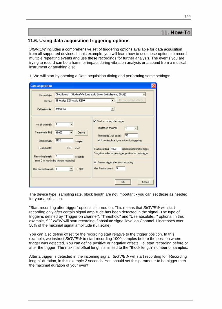
11. How-To
11.6. Using data acquisition triggering options
SIGVIEW includes a comprehensive set of triggering options available for data acquisitionfrom all supported devices. In this example, you will learn how to use these options to recordmultiple repeating events and use these recordings for further analysis. The events you aretrying to record can be a hammer impact during vibration analysis or a sound from a musicalinstrument or anything else.
1. We will start by opening a Data acquisition dialog and performing some settings:
The device type, sampling rate, block length are not important - you can set those as neededfor your application.
"Start recording after trigger" options is turned on. This means that SIGVIEW will startrecording only after certain signal amplitude has been detected in the signal. The type oftrigger is defined by "Trigger on channel", "Threshold" and "Use absolute..." options. In thisexample, SIGVIEW will start recording if absolute signal level on Channel 1 increases over50% of the maximal signal amplitude (full scale).
You can also define offset for the recording start relative to the trigger position. In thisexample, we instruct SIGVIEW to start recording 1000 samples before the position wheretrigger was detected. You can define positive or negative offsets, i.e. start recording before orafter the trigger. The maximal offset length is limited to the "Block length" number of samples.
After a trigger is detected in the incoming signal, SIGVIEW will start recording for "Recordinglength" duration, in this example 2 seconds. You should set this parameter to be bigger thenthe maximal duration of your event.
144

11. How-To
"Re-Arm..." trigger option instructs SIGVIEW to start waiting for a new trigger as soon as onerecording has been made. After SIGVIEW detects a trigger for the first time and records 2seconds of a signal it will automatically open new data acquisition window with the samesettings and will wait for another trigger in it. That way, each 2 seconds recording will remainin a separate window. You can define maximal number of such windows with the "MaxRe-Arm count".
2. Press OK in the data acquisition dialog and a signal window will open. Press "Start button"in a toolbar to start data acquisition, i.e. waiting for a trigger. Since there is still no signal,nothing will happen immediately. In the background, SIGVIEW is acquiring your signal andtesting if the trigger has occurred.
3. Now, trigger the signal event by playing some sound, impacting with a hammer or anythingelse causing the energy to be detected in the signal. SIGVIEW will start recording 1000samples before the event and the recording will last 2 seconds.
4. As soon as the recording has finished, new window will open waiting for a next trigger.Please repeat this 5 times to get 5 windows with recordings. Your SIGVIEW window shouldlook like this:
145

11. How-To
5. Now, use Window/Tile option to arrange all window. Select all signal windows in ControlWindow (Context menu/Select all window) and choose Zoom-Out function in a toolbar to seethe complete content of all signal windows. The SIGVIEW window will look like this:
6. While still in Control Window, you can apply some analysis to all 5 recordings at the sametime, for example FFT. Also, you can show all recordings in an overlay window by usingcorresponding options from a Control window's context menu.
146

KEYWORD INDEX
147
- 3 -
3D graphics types, 93D graphics, basic operations 93D graphics, types 93D signal log 93D-graphics 9
- a -
acquisition 11acquisition, sound cards 11AIFF 3alarm,with 10and zooming 9annotations, signal 1another application 2artifacts, removing 2ASCII, saving multichannel 3AU, loading 3auto scale, 3D graphics axes 9auto scale, signal coordinate 1autocorrelation 5automating SIGVIEW with 3automating, command-line 12average 10averaging, FFT 5averaging, signal 6axes settings, 3D graphics 9
- b -
bandpass, filters 6bandstop, filters 6basic concepts
- c -
calibration 115, 11changing signal values 2clipboard copying 3D 9clipboard, working with 2colors, 3D graphics 94, 96, 10command-line options 12
command-line, options 12command-line, reference 12comments in signal 1complex FFT 7confidence, test for spectral 5control window 4control window, basics 4control window, concept 4coordinate systems, signal 1copying tools, Control 4copying, from signal 2correlation, cross 6Crest factor 10cross coherence 6cross correlation 6cross gain 6cross spectrum 6cross-spectral analysis 6custom filter bank 8custom filter curve 8custom tools 3custom, tools 3cutting, from signal 2
- D -
DAQ 11data acquisition 11data log, in file 11dB, in FFT 5decibel, in FFT 5decimation, in data 11defaults, spectral analysis 5detecting peaks 7deviation, standard 10differentiate, signal 7distribution, probability 6drag 'n drop, Control Window 4draw axes, signal coordinate 1
- E -
Excel, importing data 3
exporting, window as bitmap 2extract from-to 2extract X-ruler 9extract Y-ruler 9extracting parts of the signal 2extracting signals from 3D 9
- f -
fast forward 2fft, basics 5FFT, complex 7fft, feneral information 5fft, useful links 5file formats 3file formats, supported 3file log 11file log, from data acquisition 11filter bank 8filter curve, custom 8filters 6format, files 3
- g -
gaussian noise, 7generating, signal 76, 10generator, signal, 7go to sample 2graph, analysis 4graphics 94, 9
- h -
harmonic ruler 1hiding windows 4
- I -
IFFT 8instrument log 10instruments 10instruments properties 10instruments, min max avg 10instruments, statistics 10instruments,marker, signal 10integral curve 7

inverse FFT 6inverse, fft 8
- l -
labels, signal coordinate 1linear trend, removing 6link 4links, between windows 39, 4loading signals 3loading, tools 3loading, workspace 3log, for instrument values 10logarithm, X-axis,axes 1logging data in file 11logging signals 9
- m -
marker 10maximum 10maximum position 10maximum, value in the signal 10mean frequency 10Measurement Computing, 11median 10median frequency 10min&max, signal coordinate 1minimum 10minimum position 10minimum, value in the signal 10monitoring, real-time data 11mousewheel 1moving average 6moving through signals 1MP3 3MPEG 3multiple windows operations 4
- N -
National Instruments, DAQ 11NI, DAQ 11noise signal, 7normalize (remove DC) 6
normalize, signal 7normalizing, signal 7
- o -
octave plots 8octave, 1/3 8options 12overlaying signals 1overlays 1
- p -
padding signal with zeros 5palettes 10pasting, to signal 2peak count 7peak detection 7peak hold 7peaks 5phase shift 6play signal 2play, as fast as possible 2playing signal 2positioning signal, on specific 2Power spectral density 5Power spectrum 5preview, signal coordinate 1printing, by copying to 2probability distribution 6properties,instruments 10PSD 5
- r -
range,instruments 10recording 11registration, How? 12registration, Why? 35, 12remove DC 6remove offset 6removing linear trend 6resampling 6rewind 2RMS 10ruler, signal 1ruler, using for selection 1
- s -
sample 2
sampling rate conversion 6sampling rate, resampling 6saving 3saving signals 3saving, multichannel signals 3saving, tools 3saving, workspace 3sawtooth signal 7scale, changing in signal 7scaling, signal 7scripting, command-line 12scripts, creating 12segments, selecting for FFT 6selecting, in control window 4selecting, part of the signal 1settings 13, 9showing/hiding windows 4signal averager 6signal calculator 5signal log 9signal ruler 1signals 2Sigview, general description slice extraction from 9smoothing 6sorted values curve 7sound card, acquisition 11spectrogram view 9standard deviation 10statistic, Time FFT 7step change 1stop playing 2sum 10sweep signal, 7SWS files 37, 3SWT files 3system 13, 13, 13, 13, 1
- t -
tags in signal 1Time FFT statistics 7timefft.rng file 7tools 3

trigger recording, How-To 14triggering 11triggering, How-To 14triggers 11types, 3D graphics 9types,instruments 10
- u -
unit, calibration 11units, calibration, level, signal 11unlink 4
- v -
volume, adjust automatically 2
- w -
waterfall view, switching 9WAV files, loading 3WAV, saving multichannel 3weighted mean 10weighted median 10white noise, 7Window 4windowing, in FFT 5WMA files, loading 3workspace, loading and 3
- z -
zooming, signals 1zooming, with mousewheel 1

End