Embed Size (px)
Citation preview

Side-information in Control and EstimationGovind Ramnarayan, Gireeja Ranade and Anant Sahai
Wireless Foundations, EECS, UC [email protected], [email protected], [email protected]
Abstract—As in portfolio theory, we can think of the valueof side-information in a control system as the change in the“growth rate” due to side-information. A scalar counterexample(motivated by carry-free deterministic models) shows the valueof side-information for control does not exactly parallel the valueof side-information for portfolios. Mutual-information does notseem to be a bound here.
The concept is further explored through a spinning vectorcontrol system that is re-oriented at each time so that the controlor observation direction is partially unknown. The value of side-information can be calculated in this setup and it behaves quitedifferently in a control vs. estimation context. A second exampleconsiders the problem of vector control over a (scalar) erasurechannel, the dual problem to the estimation problem of intermit-tent Kalman Filtering. The value of information here is measuredthrough the change in the critical packet-drop probability for thesystem. While non-causal side-information regarding the packetarrivals does not affect the critical probability for the estimationproblem, we find that it can generically be very valuable for thecontrol problem — it seems to change the scaling behavior forthe control counterpart to what would be considered the “highSNR limit” in communication problems.
I. INTRODUCTION
Parameter uncertainty has a long history in control theory— the very idea of robust control is about dealing with it.Recently, the advent of networked control systems has madestochastic uncertainty models more relevant. There is nowa real need to have a theory capable of dealing with side-information in control. As just one example, control theoristsare interested in knowing how networked control systemsbehave with or without acknowledgements of dropped packetssince this is relevant for choosing among practical protocolslike TCP vs. UDP [1]. Acknowledgements are a kind of side-information about control channel state, but as of now, there isno theoretical guidance for how to think about it in a principledway.
Fortunately, such things have long been studied in infor-mation theory in the context of unknown fading channels[2]. Medard in [3] examines the effect of imperfect channelknowledge on capacity, and Lapidoth and Shamai quantify thedegradation in performance due to channel-state estimationerrors by the receiver [4]. Pradhan et al. show that the dualitybetween source and channel coding in fact extends to thecase with side-information under certain conditions [5]: this isparticularly interesting given the well-known parallel betweensource coding and portfolio theory, which we will connect tohere. Further, Kotagiri and Laneman [6] study the impact ofnon-causal knowledge of the state in a multiple-access setting.There are many more interesting results as well, but spaceprecludes any serious discussion here.
Moving beyond communication, the MMSE dimensionlooks at the value of side-information in an estimation setting.In a system with only additive noise, Wu and Verdu showthat a finite number of bits of side-information regarding theadditive noise cannot generically change the high-SNR scalingbehavior of the MMSE [7]. Portfolio theory also gives us anunderstanding of side-information. The key is the doubling rateof the system, i.e. the rate at which a gambler who choosesan optimal portfolio doubles his principal. Kelly studied thisthrough bets placed on horse races in [8]. If each race outcomeis distributed according a random variable X , then the mutualinformation between X and Y , I(X;Y ), measures the gainin the doubling rate that the side-information Y provides thegambler.
Cover showed the existence of universal portfolios [9] aswell the impact of side information for these [10]. This leads toa natural question: if there exists a portfolio that can performoptimally while agnostic to the parameters of the systems,under what circumstances can we design control strategies thatwork universally? What is the parallel in control?
Control systems, like portfolios, have an underpinning ofexponential growth. Just as the investor can choose to buyand sell at each time step to maximize growth, the controllerhas the choice of control strategy to minimize growth (ormaximize decay). Further, causality and time are importantconsiderations in both portfolios and control. Directed mutualinformation captures exactly the causal information that isshared between two random variables. This connection hasbeen made explicit for portfolio theory in [11], [12] byshowing that the directed mutual information I(Xn → Y n)is the gain in the doubling rate for a gambler due to causalside information Y n. Of course, directed mutual informationis central to control and information theory as the measure ofthe capacity of a channel with feedback [13].
Here, we explore the value of both causal and non-causalside information for control systems though models that in-volve multiplicative parameter uncertainty, where these param-eters have an i.i.d. character to them. Multiplicative modelsexhibit fundamentally different behavior than additive noisemodels do. In models with additive noise, the linearity of thesystem and the linearity of expectation means that estimationand control problems reduce to each other — the optimalcontrol is a deterministic function of the optimal estimate.Multiplicative noise breaks this duality and the philosophicaldifferences in estimation and control become evident opera-tionally as well.
We start with a simple scalar example and then define
value of side-information for control in a way that parallelsinformation-theoretic portfolio theory. Then, we discuss twointeresting vector examples, the latter of which demands adifferent (coarser) way of understanding the value of side-information.
II. A SCALAR EXAMPLE AND SEMI-DETERMINISTIC STORY
This section draws heavily upon our earlier Allerton paper[14] but helps make the ideas above more concrete. Considera simple scalar control system with perfect state-observation
X[n+ 1] = α(X[n] +B[n]U [n]),
Y [n] = X[n]. (1)
Suppose B[n] are a series of i.i.d. random variables with meanµb and variance σ2
B , and X[0] ∼ N (0, 1). The system isscaled by a scalar constant factor a at each time step. Theaim is to choose U [n], a function of Y [n], so as to stabilizethe system. We can show that the system (1) is mean-squarestabilizable using linear strategies if limn→∞ E[X[n]2] < ∞if α2 <
(µ2B+σ2
B
σ2B
).
The growth rate of the system we are considering aboveis related to the flow of information through the system:the randomness in the control parameter B[n] impedes thecontroller’s ability to stabilize the system. Recent works haveshown that a deterministic bit-level perspective (a la [15], [16],[17]) on control systems can help elucidate the informationflows in the system [18], [19].
+
+
+
+
+
?
?
?
?
Ber(.5)
Ber(.5)
u[n]
b1[n] = 1
x[n + 1]b[n]u[n]
X
(a)
+
+
+
+
+
?
?
u[n]
b1[n] = 1
x[n + 1]b[n]u[n]
X X
?
b0[n] = 0
(b)
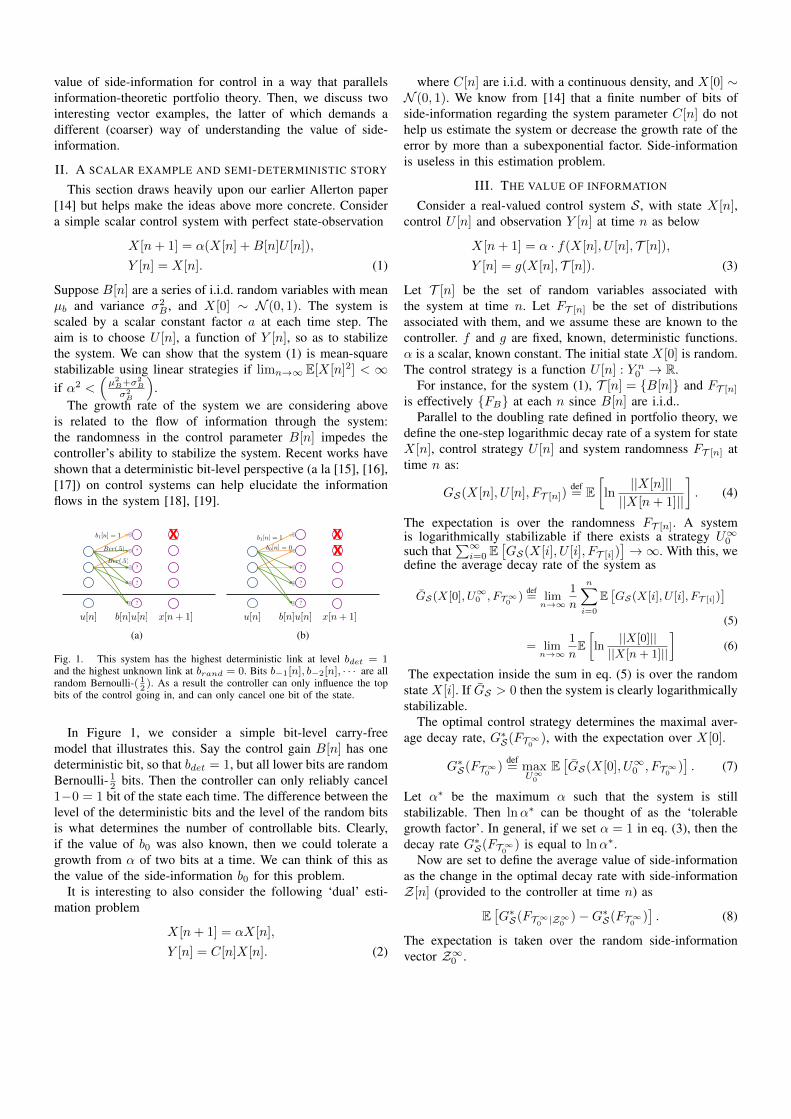
Fig. 1. This system has the highest deterministic link at level bdet = 1and the highest unknown link at brand = 0. Bits b−1[n], b−2[n], · · · are allrandom Bernoulli-( 1
2). As a result the controller can only influence the top
bits of the control going in, and can only cancel one bit of the state.
In Figure 1, we consider a simple bit-level carry-freemodel that illustrates this. Say the control gain B[n] has onedeterministic bit, so that bdet = 1, but all lower bits are randomBernoulli- 12 bits. Then the controller can only reliably cancel1−0 = 1 bit of the state each time. The difference between thelevel of the deterministic bits and the level of the random bitsis what determines the number of controllable bits. Clearly,if the value of b0 was also known, then we could tolerate agrowth from α of two bits at a time. We can think of this asthe value of the side-information b0 for this problem.
It is interesting to also consider the following ‘dual’ esti-mation problem
X[n+ 1] = αX[n],
Y [n] = C[n]X[n]. (2)
where C[n] are i.i.d. with a continuous density, and X[0] ∼N (0, 1). We know from [14] that a finite number of bits ofside-information regarding the system parameter C[n] do nothelp us estimate the system or decrease the growth rate of theerror by more than a subexponential factor. Side-informationis useless in this estimation problem.
III. THE VALUE OF INFORMATION
Consider a real-valued control system S, with state X[n],control U [n] and observation Y [n] at time n as below
X[n+ 1] = α · f(X[n], U [n], T [n]),
Y [n] = g(X[n], T [n]). (3)
Let T [n] be the set of random variables associated withthe system at time n. Let FT [n] be the set of distributionsassociated with them, and we assume these are known to thecontroller. f and g are fixed, known, deterministic functions.α is a scalar, known constant. The initial state X[0] is random.The control strategy is a function U [n] : Y n0 → R.
For instance, for the system (1), T [n] = {B[n]} and FT [n]
is effectively {FB} at each n since B[n] are i.i.d..Parallel to the doubling rate defined in portfolio theory, we
define the one-step logarithmic decay rate of a system for stateX[n], control strategy U [n] and system randomness FT [n] attime n as:
GS(X[n], U [n], FT [n])def= E
[ln||X[n]||||X[n+ 1]||
]. (4)
The expectation is over the randomness FT [n]. A systemis logarithmically stabilizable if there exists a strategy U∞0such that
∑∞i=0 E
[GS(X[i], U [i], FT [i])
]→∞. With this, we
define the average decay rate of the system as
GS(X[0], U∞0 , FT∞0
)def= lim
n→∞
1
n
n∑i=0
E[GS(X[i], U [i], FT [i])
](5)
= limn→∞
1
nE[ln
||X[0]||||X[n + 1]||
](6)
The expectation inside the sum in eq. (5) is over the randomstate X[i]. If GS > 0 then the system is clearly logarithmicallystabilizable.
The optimal control strategy determines the maximal aver-age decay rate, G∗S(FT∞
0), with the expectation over X[0].
G∗S(FT∞0
)def= max
U∞0
E[GS(X[0], U∞0 , FT∞
0)]. (7)
Let α∗ be the maximum α such that the system is stillstabilizable. Then lnα∗ can be thought of as the ‘tolerablegrowth factor’. In general, if we set α = 1 in eq. (3), then thedecay rate G∗S(FT∞
0) is equal to lnα∗.
Now are set to define the average value of side-informationas the change in the optimal decay rate with side-informationZ[n] (provided to the controller at time n) as
E[G∗S(FT∞
0 |Z∞0
)−G∗S(FT∞0
)]. (8)
The expectation is taken over the random side-informationvector Z∞0 .

+
+
+
+
+
?
?
?
?
u[n]
b1[n] = 1
x[n + 1]b[n]u[n]
X b�1[n] = 1
(a)
+
+
+
+
+?
u[n]
b1[n] = 1
x[n + 1]b[n]u[n]
X X X
b0[n] = 0
b�1[n] = 1
(b)
Fig. 2. Consider the following gain for the controller in (a): b1[n] =1, b−1[n] = 1 are deterministically known, but all other links are Bernoulli-(.5). Only a gain of logα = 1 can be tolerated in this case. Now, say side-information regarding the value of b0[n] is received as in (b). This suddenlybuys the controller not just one, but two bits of growth.
Note that in the carry-free model in Fig. 1, one extra bitof information about b0 increases the tolerable growth of thesystem by exactly one bit. What is the potential value of R-bits of side-information? This is the answer to the optimizationproblem
VS(R)def= max
I(T [n];Z[n])=R ∀nE[G∗S(FT∞
0 |Z∞0
)−G∗S(FT∞0
)]. (9)
Finally, we also define a corresponding decay rate for esti-mation. For the system S:
X[n+ 1] = α · f(X[n], T [n]),
Y [n] = g(X[n], T [n]), (10)
we define the one-step logarithmic error decay rate as
GS(X[n], FT [n])def= E
[ln
||X[n]− X[n]||||X[n+ 1]− X[n+ 1]||
]. (11)
The average logarithmic decay rate can then be defined as inthe control case.
A. A control counterexample
In the portfolio theory literature, it is known that themaximum increase in doubling rate due to side-informationZ for a set of stocks distributed as T is upper bounded byI(T ;Z). With our observation about deterministic models itis tempting to conjecture that “a bit buys a bit” and a similarbound holds for the value of information in control systems.However, we see that the following counterexample rejectsthis conjecture. Consider the carry-free model in Fig. 2. InFig. 2(a) the uncertainty in b0[n] does not allow the controllerto utilize the knowledge that b−1[n] = 1. However, one bitof information b0[n] in Fig. 2(b), lets the controller buy twobits of gain in the tolerable growth rate as explained in thecaption. In the case of portfolio theory, it is possible to hedgeacross uncertainty in the system and get “partial-credit” foruncertain quantities. This is not possible in communication1
1It seems that the ‘commitment’ challenge that is faced by control canalso be seen in communication systems, where it is also not possible tohedge across realizations. Consider a “compound” channel made of two R-bit channels A and B but with distinct inputs, so only one can be used at atime. The message sent across one of the channels is randomly erased withprobability 0.5. In this case, one bit of side-information about which channelis to be erased can buy us more than a bit: we get R
2bits of message on
average.
✓n
(a)
✓n
Q1Q2
(b)
Fig. 3. A spinning control setup: the target can be moved only along therandomly chosen control direction. In version (a), the controller has perfectaccess to the control direction, while in version (b) only a quantized versionis available.
and control systems since it is not possible to hedge a controlsignal in the same way one can hedge a bet.
IV. A SPINNING SYSTEM
The first example here highlights the difference in the im-pact of side-information for control and estimation problems.
A. A spinning controller: the control case
Consider the noiseless 2D control system S in (12)[X1[n+ 1]X2[n+ 1]
]= α
([X1[n]X2[n]
]+ U [n]
[cos θnsin θn
]),
Y [n] =
[X1[n]X2[n]
]. (12)
The controller has perfect access to the system state, butis subject to the following limitation: at each time n, thecontrol direction is determined by a random spin, i.e. thecontroller may only act along the direction
[cos θn sin θn
]T,
where θn is drawn uniformly from [0, 2π]. Information aboutthe control direction, θn, is revealed to the controller beforeit chooses U [n]. The initial state
[X1[0]X2[0]
]Tis drawn
randomly according to some distribution, and the goal is todrive the state to the origin. After the control acts, the systemis spun again so that only the distance of the target from theorigin is preserved, and the scale α is applied. This is depictedin Fig. 3(a).
Consider the case where no information about the controldirection θn is revealed to the controller before acting, i.e.the controller has 0 bits of information about the systemrandomness. Clearly, in this case the optimal control actionU [n] = 0, and no growth α can be tolerated. The system isonly stable if α ≤ 1. For the other extreme case, where thecontroller knows the present control direction perfectly, thefollowing theorem characterizes the optimal strategy.
Theorem 4.1: The optimal control for the system (12) isgiven by the greedy strategy, i.e. U∗[n] = −X1[n] cos θn −X2[n] sin θn for all n.
The proof follows using dynamic programming.Corollary 4.2: The logarithmic decay rate for system (12)
with perfect information at each time n about θn is ln 2, andthe tolerable growth rate is thus α∗ = 2.

Proof: The logarithmic decay rate of the system for theoptimal control is given by
1
π
∫ π
0
1
2ln
|X1[0]|2 + |X2[0]|2
|X1[0] cos θ −X2[0] sin θ|2dθ (13)
This integral evaluates to ln 2, and hence α∗ = 2.
B. Partial side-information
The symmetric randomness in this example makes is easy toevaluate the impact of side-information regarding the controlrandomness. Instead of perfect side-information, what happenswhen the controller has access to only two bits of informationabout the control direction?
Consider the space divided into quadrants, and only thequadrant containing the direction will be revealed at time n.Say only the quadrant of the control direction θn, Q1 or Q2,is revealed to the controller at time n (Fig. 3(b)).
Theorem 4.3: The logarithmic decay rate with two bits ofside-information for the system (12) is at least .47, and thetolerable growth rate is thus at least α = 1.61.
This also follows using dynamic programming. Similar re-sults for k-bits of side-information are summarized in Table I.Just three bits of side-information gets the tolerable growthrate pretty close to the case of perfect side-information.
TABLE ISYSTEM GROWTH AS A FUNCTION OF STATE-INFORMATION
Side-info Decay rate Tolerable growth0 bits 0 11 bit 0.200 1.222 bits 0.477 1.613 bits 0.624 1.86∞ bits ln 2 2
Note that even in the presence of noisy information aboutthe control direction it is possible to stabilize the system forcertain growth rates α. This parallels the result in [14].
C. A spinning observer: the estimation case
The behavior of the corresponding estimation problempresents a sharp contrast to the control problem. Consider thesystem below, where the observation directions θn are random[
X1[n+ 1]X2[n+ 1]
]= α
[X1[n]X2[n]
],
Y [n] =[cos θn sin θn
] [X1[n]X2[n]
]. (14)
If θn is perfectly known to the observer, the estimation errorgoes to zero after the first two observations. So the logarithmicdecay rate of the error with perfect information is infinity,unlike the control case which has a small finite decay rate.
Surprisingly, the two-step observability result is quite frag-ile. We know from the arguments in [14] that even a slightcontinuous uncertainty regarding θn renders the estimationproblem impossible. The error is not shrinking with time.Partial side-information is no more useful than no side-information at all.
V. AN INTERMITTENT CONTROLLER
This section considers the control problem that is the dual ofthe intermittent Kalman filtering problem [20]. In [21], Mo andSinopoli found two interesting examples that defined cornercases for the critical erasure probability for the estimationproblem. Building on this, Park and Sahai characterized thedifference in the critical drop probability in the presence andabsence of eigenvalue cycles [22]. The control counterpart isdefined below:[
X1[n+ 1]X2[n+ 1]
]=
[λ1 00 λ2
] [X1[n]X2[n]
]+ U [n]β[n]
[11
],
Y [n] =
[X1[n]X2[n]
]. (15)
Let λmax = |λ1| ≥ |λ2| ≥ 1, and β[n] is a Bernoulli-(p)random variable. We use the terminology ‘control arrival’ inthe event that β[n] = 1. [23] showed that this system canbe mean-square stabilized by an LTI controller if and only if1− p < 1
(λ1λ2)2.
Here, we investigate the impact of partial non-causal side-information about control arrivals on the critical probability.The logarithmic decay rate of the system does not serveas a good measure in this problem since the probability ofthe system state eventually being set to zero is 1, but theinteresting question is that of the rate of decay. The changein the critical probability can be thought of as a proxy for thevalue of side-information and we explore how it changes.
Non-causal look-ahead regarding the sequence β[n] does notchange the critical probability for the observation problem.We are interested in understanding the effect of this side-information for the control problem.
Our first observation is to note that with infinite look-aheadon the sequence β[n], the controller is able to plan for futurearrivals and will be able to set the state to zero on the secondarrival.
Theorem 5.1: The critical probability for the control prob-lem eq. (15) is 1
λ2max
.The proof follows from a time-reversal argument: the con-
trol problem is the same as the observation problem if timeis reversed and we are only waiting on the first two arrivals.The result follows from arguments in [24].
With this background, we consider the case with λ1 = 2and λ2 = −2. These eigenvalues form a cycle of periodtwo. We can further separate out the angle and the mag-nitude of the eigenvalues and write the gain matrix A =
2
[1 00 −1
].[1 00 −1
]is a matrix that rotates a vector by π
2 ,
and[1 00 −1
]2=
[1 00 1
]is the identity matrix.
Theorem 5.2: A greedy control strategy thatprojects the state vector in the control directionU [n] = −
[2 −2
] [X1[n]X2[n]
]Tis the optimal strategy.
The basic idea is that controls applied at even and odd timescannot substitute for each other and one of each is essential.
These arguments for the 2D-case generalize to systems ofdimension-k with an eigenvalue cycle of period-k and the same

results hold: the estimation critical probability and the controlcritical probability are exactly the same. Further, since thestrategy is time-invariant, non-causal knowledge of the patternof arrivals would have no impact on the rate of the decay ofthe system state. Here, side-information has no value.
On the other hand, consider a general aperiodic system.The optimal strategy in this case is unclear without any look-ahead, however, we can implement a finite-horizon dynamicprogramming solution to the problem to numerically evaluatethe critical probability for a given system. This is exploredin Fig. 4, where the critical probabilities for the problem areplotted against the maximum eigenvalue. The first interestingobservation is that the optimal dynamic programming solutionwith no look-ahead decays exactly as the optimal LTI strategy:the lines for 1
(λ1λ2)2and the optimal dynamic programming
strategy (q = 0) are on top of each other [25].With infinite look-ahead, the critical probability decays as1
λ2max
, which is the topmost line. To understand the behaviorin between, we plot the the strategy with one-step look-aheadat each time (q = 1), and one-step look-ahead with probabilityhalf (q = 0.5). The optimal dynamic programming strategiesare compared to a simple align-and-kill strategy (AK) thatassumes that the next control will arrive. The strategies seemto converge at high eigenvalues and this warrants furtherexploration. That the slopes are different suggests that the side-information has a scaling effect on the mapping between theeigenvalues and the critical erasure probability.
The change in the slopes of the curves shows that channelpredictability gets more valuable with increasing eigenvalues.A system designer might prefer a noisier but more predictablechannel, even though it has lower anytime reliability. Incontrast to the observation problem, knowledge of futurecontrol directions seems to be the useful side-information forthe general aperiodic control problem.
æ
æ
æ
æ
æ
æ
à
à
à
à
à
à
ì
ì
ì
ì
ì
ì
ò
ò
ò
ò
ò
ò
ô
ô
ô
ô
ô
ô
ç
ç
ç
ç
ç
ç
á
á
á
á
á
á
í
í
í
í
í
í
A-K q=0
A-K q=0.5
A-K q=1
DP q=0
DP q=0.5
DP q=1
1 � Λ22
1 � HΛ1 Λ2L2
1 � Λ22
A-K q=0
A-K q=0.5A-K q=1
DP q=0.5
DP q=1
DP q=0, 1 � HΛ1 Λ2L2
1.3 2 3.9 6.5 9.1 13Λ2
10-4
0.001
0.01
0.1
1
Critical drop probability
Fig. 4. Critical erasure probability vs. mag. of max eigenvalue λ1λ2
= 1.18.
ACKNOWLEDGMENTS
The authors would like to thank the NSF for a GRF andCNS-0932410, CNS-1321155, and ECCS-1343398.
REFERENCES
[1] L. Schenato, B. Sinopoli, M. Franceschetti, K. Poolla, and S. S.Sastry, “Foundations of control and estimation over lossy networks,”Proceedings of the IEEE, vol. 95, no. 1, pp. 163–187, 2007.
[2] A. Lapidoth and P. Narayan, “Reliable communication under channeluncertainty,” Information Theory, IEEE Transactions on, vol. 44, no. 6,pp. 2148–2177, 1998.
[3] M. Medard, “The effect upon channel capacity in wireless communica-tions of perfect and imperfect knowledge of the channel,” InformationTheory, IEEE Transactions on, vol. 46, no. 3, pp. 933–946, 2000.
[4] A. Lapidoth and S. Shamai, “Fading channels: how perfect need perfectside information be?” IEEE Transactions on Information Theory, vol. 48,no. 5, pp. 1118–1134, 2002.
[5] S. S. Pradhan, J. Chou, and K. Ramchandran, “Duality between sourcecoding and channel coding and its extension to the side informationcase,” Information Theory, IEEE Transactions on, vol. 49, no. 5, pp.1181–1203, 2003.
[6] S. Kotagiri and J. Laneman, “Multiaccess channels with state knownto some encoders and independent messages,” EURASIP Journal onWireless Communications and Networking, vol. 2008, pp. 1–14, 2008.
[7] Y. Wu and S. Verdu, “MMSE dimension,” Information Theory, IEEETransactions on, vol. 57, no. 8, pp. 4857–4879, 2011.
[8] J. Kelly Jr, “A new interpretation of information rate,” InformationTheory, IRE Transactions on, vol. 2, no. 3, pp. 185–189, 1956.
[9] T. M. Cover, “Universal portfolios,” Mathematical finance, vol. 1, no. 1,pp. 1–29, 1991.
[10] T. M. Cover and E. Ordentlich, “Universal portfolios with side infor-mation,” Information Theory, IEEE Transactions on, vol. 42, no. 2, pp.348–363, 1996.
[11] H. H. Permuter, Y.-H. Kim, and T. Weissman, “On directed informationand gambling,” in Information Theory, 2008. ISIT 2008. IEEE Interna-tional Symposium on. IEEE, 2008, pp. 1403–1407.
[12] ——, “Interpretations of directed information in portfolio theory, datacompression, and hypothesis testing,” Information Theory, IEEE Trans-actions on, vol. 57, no. 6, pp. 3248–3259, 2011.
[13] S. Tatikonda, “Control under communication constraints,” 2000.[14] G. Ranade and A. Sahai, “Non-coherence in estimation and control,”
in 51th Annual Allerton Conference on Communication, Control, andComputing, 2013.
[15] A. Avestimehr, S. Diggavi, and D. Tse, “Wireless network informationflow: A deterministic approach,” Information Theory, IEEE Transactionson, vol. 57, no. 4, pp. 1872–1905, 2011.
[16] U. Niesen and M. Maddah-Ali, “Interference alignment: From degrees-of-freedom to constant-gap capacity approximations,” in InformationTheory Proceedings (ISIT), IEEE International Symposium on, 2012,pp. 2077–2081.
[17] S. Park, G. Ranade, and A. Sahai, “Carry-free models and beyond,” inIEEE International Symposium on Information Theory, 2012, pp. 1927–1931.
[18] P. Grover and A. Sahai, “Implicit and explicit communication in decen-tralized control,” in 48th Annual Allerton Conference on Communica-tion, Control, and Computing, Monticello, Illinois., 2010.
[19] S. Y. Park and A. Sahai, “It may be easier to approximate decentralizedinfinite-horizon LQG problems,” in Decision and Control (CDC), IEEE51st Annual Conference on, 2012, pp. 2250–2255.
[20] B. Sinopoli, L. Schenato, M. Franceschetti, K. Poolla, M. I. Jordan, andS. S. Sastry, “Kalman filtering with intermittent observations,” AutomaticControl, IEEE Transactions on, vol. 49, no. 9, pp. 1453–1464, 2004.
[21] Y. Mo and B. Sinopoli, “A characterization of the critical value forKalman filtering with intermittent observations,” in Decision and Con-trol, CDC. 47th IEEE Conference on, 2008, pp. 2692–2697.
[22] S. Park and A. Sahai, “Intermittent Kalman filtering: Eigenvalue cyclesand nonuniform sampling,” in American Control Conference (ACC),2011, 2011, pp. 3692–3697.
[23] N. Elia, “Remote stabilization over fading channels,” Systems & ControlLetters, vol. 54, no. 3, pp. 237–249, 2005.
[24] S. Y. Park, “Information flow in linear systems,” Ph.D. dissertation,University of California, Berkeley, December 2013.
[25] O. C. Imer, S. Yuksel, and T. Basar, “Optimal control of LTI systemsover unreliable communication links,” Automatica, vol. 42, no. 9, pp.1429–1439, 2006.