Siddhartha Karmakar and Subhendu Rakshity - arXiv · Higher dimensional operators in 2HDM Siddhartha Karmakar and Subhendu Rakshity Discipline of Physics, Indian Institute of Technology

Higher dimensional operators in 2HDM

Siddhartha Karmakar∗ and Subhendu Rakshit†

Discipline of Physics, Indian Institute of Technology Indore,

Khandwa Road, Simrol, Indore - 453 552, India

Abstract

We present a complete (non-redundant) basis of CP- and flavour-conserving six-dimensional

operators in a two Higgs doublet model (2HDM). We include Z2-violating operators as well. In such

a 2HDM effective field theory (2HDMEFT), we estimate how constraining the 2HDM parameter

space from experiments can get disturbed due to these operators. Our basis is motivated by the

strongly interacting light Higgs (SILH) basis used in the standard model effective field theory

(SMEFT). We find out bounds on combinations of Wilson coefficients of such operators from

precision observables, signal strengths of Higgs decaying into vector bosons etc. In 2HDMEFT, the

2HDM parameter space can play a significant role while deriving such constraints, by leading to

reduced or even enhanced effects compared to SMEFT in certain processes. We also comment on

the implications of the SILH suppressions in such considerations.

∗ E-mail: [email protected]† E-mail: [email protected]

1

arX

iv:1

707.

0071

6v2

[he

p-ph

] 2

2 Se

p 20

17

I. INTRODUCTION

Two Higgs doublet model is the most studied extension of the scalar sector of the Standard

model (SM) of particle physics. Inclusion of an additional scalar doublet is necessary in the

supersymmetric models. There are other phenomenological motivations for considering non-

supersymmetric versions of this model as well. For example, an additional Higgs doublet can

lead to a successful electroweak baryogenesis [1]. Moreover, anomalies in tauonic B-decays

can be addressed in a 2HDM [2–4].

Non-observation of new fundamental particles at the LHC motivates us to formulate

the SM effective Lagrangian below a TeV or so. The recent data implies that the newly-

discovered 125 GeV Higgs boson is SM-like, but still allows for the existence of new scalars

at sub-TeV scales. In the alignment limit, 2HDM can accommodate such new scalars so

that the extra contributions coming from the renormalisable 2HDM Lagrangian to various

processes involving SM particles are reasonably small. This calls for an extensive study of

higher dimensional operators in exploring 2HDM phenomenology as their effects can be of

the same order of the extra contribution in 2HDM at the tree-level in the alignment limit.

In this paper, we formulate a basis of independent six-dimensional (6-dim) operators

assuming 2HDM to be the low-energy theory. We include the Z2-violating operators, but, for

simplicity, exclude the CP- and flavour-violating ones. The bounds imparted on the Wilson

coefficients by the electroweak precision tests (EWPT) are estimated. Such operators also

affect the signal strengths of the SM-like Higgs boson decaying into a pair of vector bosons.

We estimate such contributions as in future, better measurements of these signal strengths

can further tighten constraints on these Wilson coefficients. Our results also reflect the fact

that the inclusion of higher dimensional operators can relax the bounds on the parameter

space of renormalisable 2HDM. We also discuss the cases where we have weighed the Wilson

coefficients following the SILH prescription as in the SMEFT [5] and mark the resulting

changes in the above-mentioned bounds.

The study of a complete set of higher dimensional operators of SM goes long back [6, 7],

where the authors formulated the basis of 6-dim operators of SM assuming lepton and baryon

number conservation. A systematic study of the electroweak precision constraints on the

Wilson coefficients of the bosonic 6-dim operators was first done in the framework of the

2

so-called HISZ basis of SMEFT [8]. The problem of writing a complete set of 6-dim operators

of SMEFT was revisited in Ref. [9] where the equations of motions (EoM) of all the fields

were used to identify 21 redundant operators in the basis of Ref. [6]. The basis for SMEFT

introduced by the latter is often referred to as the Warsaw basis. The SILH basis [5] was

formulated in the context of scenarios where the hierarchy problem is alleviated due to the

existence of a strongly-interacting sector beyond the TeV scale. There are two broad classes

of models which can be represented by the SILH Lagrangian. First, the extra-dimensional

models where the Higgs boson is a part of the bulk and the rest of the SM fields are part

of a brane at low-energy [10]. The other one consists of all the models where the Higgs is

a pseudo Nambu-Goldstone boson (pNGB) of the strong sector. The Little Higgs [11] is an

archetype of the latter class. The composite Higgs models can be a part of both the classes.

The SILH Lagrangian is described by two scales of new physics, namely f , the compositeness

scale and mρ ∼ gρf , the lightest vector boson mass in the strongly-interacting sector, with

gρ being the coupling of new strong sector. An updated review of the study of SMEFT in

light of precision electroweak and Higgs signal strength data can be found in Refs. [12, 13].

The study of a composite 2HDM in the context of a SO(6)/SO(4) × SO(2) coset was

performed in Ref. [14]. Perturbative unitarity bounds on S-matrix elements were extracted

and collider phenomenology of this particular model has been explored only recently [15–17].

The 2HDM in a Little Higgs scenario was studied in Refs. [18, 19]. A few other studies of

the composite inert doublet model of dark matter have been carried out as well [20, 21].

In Ref. [22], an extension of SMEFT SILH basis incorporating a light singlet scalar along

with SM degrees of freedom was introduced. Impact of some of the six-dimensional operators

involving two Higgs doublets on exotic decay channels of charged Higgs boson were studied

in Ref. [23]. The kinetic terms comprising of four scalars and two derivatives in a N-Higgs

doublet scenario were studied recently in Refs. [24–26]. An attempt to write down the full

set of 6-dim operators in 2HDM was made in Ref. [27] in a Warsaw-like basis. In contrary,

our basis is motivated by the SILH basis in SMEFT and is a complete one, as we point out

that there is a redundant operator in the basis of Ref. [27]. In addition, as we mentioned

earlier, we include the Z2-violating operators as well.

We start with introducing the tree level Lagrangian in 2HDM and the corresponding

equations of motion and then formulate our basis in Section II. In Section III, we carry

3

out the kinetic and mass diagonalisations of the scalar fields which enable us to write down

the effective couplings of those scalars with the vector bosons. Section IV deals with the

constraints on the Wilson coefficients coming from the EWPT. In section V, we evaluate the

decay widths and signal strengths of the SM Higgs boson decaying into vector boson pairs.

Finally in Section VI we consolidate our results and eventually conclude.

II. CONSTRUCTION OF THE 2HDMEFT

A. The 2HDM Lagrangian and classical EoMs

We use the same notation as in Ref. [27] in order to avoid further confusion. The Higgs

fields in the doublet notation can be written as:

ϕI =

φ+I

1√2(vI + ρI) + i ηI

(2.1)

where I = 1, 2. Before the two Higgs fields ϕ1, ϕ2 get vacuum expectation values (vev) the

renormalisable 2HDM Lagrangian is given by:

L(4)2HDM = −1

4GaµνG

aµν − 1

4W iµνW

iµν − 1

4BµνB

µν + |Dµϕ1|2 + |Dµϕ2|2 − V (ϕ1, ϕ2)

+ i (q /Dq + l /Dl + u /Du+ d /Dd) + LY , (2.2)

where the first three are field strengths of the gauge bosons of SU(3)C , SU(2)L and U(1)Y

respectively. The indices a = 1, .., 8 and i = 1, 2, 3 are summed over. The tree-level 2HDM

potential is given by:

V (ϕ1, ϕ2) = m211|ϕ1|2 +m2

22|ϕ2|2 − (m212ϕ†1ϕ2 + h.c.) + λ1|ϕ1|4 + λ2|ϕ2|4 + λ3|ϕ1|2|ϕ2|2

+ λ4|ϕ†1ϕ2|2 +λ5

2((ϕ†1ϕ2)2 + h.c.) + (λ6|ϕ1|2 + λ7|ϕ2|2)(ϕ†1ϕ2 + h.c.). (2.3)

The term with coefficient m212 is called the soft Z2-violating term, whereas the ones with λ6

and λ7 are called the hard Z2-violating terms as they give rise to quadratically divergent

contribution to ϕ1 − ϕ2 mixing. However, one is allowed to start with non-zero values of

λ6 and λ7 as long as they can be rotated to λ6, λ7 = 0 using reparametrisation transfor-

mations [28, 29]. This scenario is referred to as “hidden soft Z2-violation”. Moreover, in

4

SILH scenarios, one considers the existence of a strongly-interacting sector at ∼ O(1 TeV)

which deliver Higgs as a pNGB at low energy. In those cases new resonances at or above

∼ O(1 TeV) take care of the quadratic divergence of Higgs mass, solving the hierarchy prob-

lem. The same mechanism will take care of the quadratic divergence in ϕ1 − ϕ2 mixing

caused by λ6 and λ7 for the 2HDMs which are governed by such a strongly-coupled sector at

higher energies. That is why in this paper we carry out all calculations keeping λ6, λ7 6= 0.

The same explanation holds true for the inclusion of Z2-odd higher dimensional operators.

The general Yukawa Lagrangian is given by,

LY = −∑I=1,2

Y eI l eϕI −

∑I=1,2

Y dI q dϕI −

∑I=1,2

Y uI q uϕI . (2.4)

For eliminating the redundant operators from the basis of 6-dim operators, one needs to

derive the EoMs of the bosonic fields from the tree-level 2HDM Lagrangian. It is necessary to

separate out the redundant ones because they do not contribute to the S-matrix elements [30].

While doing that, we neglect the five-dimensional operators [9]. The EoMs are given as:

�ϕi1 = −m211ϕ

i1 −m2

12ϕi2 − 2λ1|ϕ1|2ϕi1 − λ3|ϕ2|2ϕi1 − λ4(ϕ†2ϕ1)ϕi2 − λ5(ϕ†1ϕ2)ϕi2

−((λ6ϕ†1ϕ2 + λ∗6ϕ

†2ϕ1)ϕi1 + λ6|ϕ1|2ϕi2)− λ7|ϕ2|2ϕi2 − Y

d†1 dqi − Y e†

1 eli + Y u1 ε

ij qju,

�ϕi2 = −m222ϕ

i2 −m2∗

12ϕi2 − 2λ2|ϕ2|2ϕi2 − λ3|ϕ1|2ϕi2 − λ4(ϕ†1ϕ2)ϕi1 − λ5(ϕ†2ϕ1)ϕi1

−λ6|ϕ1|2ϕi1 − ((λ7ϕ†1ϕ2 + λ∗7ϕ

†2ϕ1)ϕi2 + λ7|ϕ2|2ϕi1)− Y d†

2 dqi − Y e†2 eli + Y u

2 εij qju,

∂ρBρµ = g′( ∑I=1,2

YϕI ϕ†I i↔Dµ ϕI +

∑ψ=q,l,u,d,e

Yψψ γµψ),

DρW iρµ =

g

2

( ∑I=1,2

ϕ†I i↔Dµ ϕI + l γµ τ

i l + q γµ τi q). (2.5)

B. Operator basis

In the universal theories [31], the deviations of the properties of the Higgs boson from

SM can be expressed in terms of only the higher-dimensional bosonic operators. Both the

Warsaw basis [9] and SILH basis [5] are bosonic bases, i.e., all bosonic operators are kept

in those bases. The effects of the 14 bosonic operators on Higgs physics were discussed in

context of the SILH basis [32], where the RG evolutions of their Wilson coefficients were

also studied. It was pointed out that the 14 operators capture all the new physics effects

5

of the Higgs sector in the SILH basis; but it takes more than 14 operators to express the

same effects in the Warsaw basis. Moreover, the study of the RG analysis of the Wilson

coefficients also implied that in SILH basis, the tree-level and loop-level operators do not

mix under running, which is not the case for the Warsaw basis. In principle, all the bases

are equivalent if they are complete and non-redundant. However, the new physics effects in

the Higgs sector are expressed with a fewer number of operators in the SILH basis compared

to the Warsaw one. This gives the SILH basis some advantage over the Warsaw basis as far

as the Higgs physics is concerned.

Now we present all the operators upto dimension six in our basis of 2HDMEFT, which is

motivated by the SILH basis of SMEFT. After including these operators the total Lagrangian

looks like:

L = L(4)2HDM + L(5) + L(6), (2.6)

where, L(5) consists of three operators, O(5)ij = (ϕi

† l)TC(ϕj† l) with i, j = 1, 2, and,

L(6) = Lϕ4D2 + Lϕ2D2X + Lϕ2X2 + Lϕ6 + Lϕ3ψ2 + Lϕ2ψ2D + Lϕψ2X + LD2X2 + Lψ4 .

(2.7)

We have defined our notation as follows: ϕ, ψ and X stand for the two scalar doublets,

fermions and gauge field strength tensors respectively. D stands for a derivative. Throughout

this paper, we have worked under the definition of L ⊃ ci(Oi/Λ2), which means all the Wilson

coefficients are named according to the suffix of the corresponding operator. For example,

cBij is the Wilson coefficient of OBij. We have incorporated the Z2-violating operators along

with the Z2-conserving ones, which was not the case for Ref. [27]. So the total number

of operators in our basis is more than that of Ref. [27]. We have marked the Z2-violating

operators in blue colour. The suppressions of these operators in a SILH scenario are given

in Appendix A.

• ϕ4D2

The ϕ4D2 operators in our basis are given in Table I. The operators O(1)21(2), O(1)12(2),

O(1)22(1), O(2)11(2) are common to both our basis and the basis introduced in Ref. [27]. OH1H12,

OH2H12, OT4 and OT5 will not appear in the basis if one demands the Z2 symmetry to be

conserved in the 6-dim Lagrangian, which is the case for Ref. [27]. In absence of these two

operators, the number of operator in our basis is 11 compared to 12 of Ref. [27]. We will

6

keep these Z2-violating operators following the logic of Section II A. The transformations

ϕ4D2

OH1 = (∂µ|ϕ1|2)2 OT1 = (ϕ†1↔Dµϕ1)2 O(1)21(2) = (ϕ†1Dµϕ2)(Dµϕ†1ϕ2)

OH2 = (∂µ|ϕ2|2)2 OT2 = (ϕ†2↔Dµϕ2)2 O(1)12(2) = (ϕ†1Dµϕ1)(Dµϕ†2ϕ2)

OH1H2 = ∂µ|ϕ1|2∂µ|ϕ2|2 OT3 = (ϕ†1↔Dµϕ2)2 + h.c. O(1)22(1) = (ϕ†1Dµϕ2)(Dµϕ†2ϕ1)

OH12 = (∂µ(ϕ†1ϕ2 + h.c.))2 OT4 = (ϕ†1↔Dµϕ2)(ϕ†1

↔Dµϕ1) + h.c. O(2)11(2) = (ϕ†2Dµϕ1)(Dµϕ†1ϕ2)

OH1H12 = ∂µ|ϕ1|2∂µ(ϕ†1ϕ2 + h.c.) OT5 = (ϕ†1↔Dµϕ2)(ϕ†2

↔Dµϕ2) + h.c.

OH2H12 = ∂µ|ϕ2|2∂µ(ϕ†1ϕ2 + h.c.)

TABLE I. Operators in Lϕ4D2 .

from the basis of Ref. [27] to our basis are:

OH1 = T−Q(1)1�D ,

OH2 = T−Q(2)2�D ,

OH12 = T + E + 2(Q12(12)ϕD +Q

12(21)ϕD ),

OH1H2 = T−Q(1)2�D = T−Q(2)1

�D ,

OT i = T + E +OHi − 4Q(i)iiiϕD ,

OT3 = T + E− 4O(1)21(2) − 2Q12(12)ϕD , (2.8)

where i = 1, 2 and T denotes total derivative terms containing ϕ and D and E stands for

the ϕ4, ϕ6 and ϕ3ψ2 terms which are already included in the basis. In the above, the fourth

transformations in eqn. (2.8) points to the fact that there is one redundant operator in the

basis of Ref. [27].

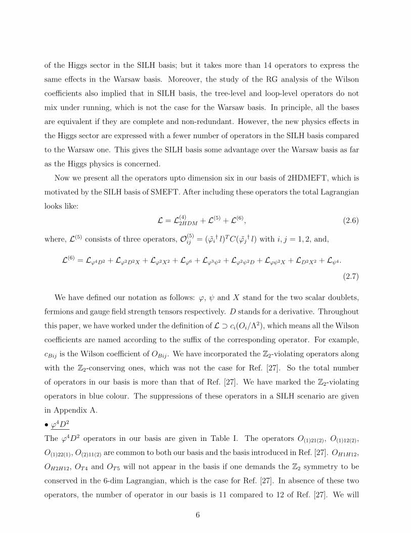
• ϕ2D2X

We have included 12 operators of class ϕ2D2X, which were not there in Ref. [27] and are

listed in Table II. We have traded 6 operators of the class ϕ2D2X for 6 operators of class

ϕ2X2, according to the relations:

OBij = T +OϕBij +1

4(OWBij +OBBij)

OWij = T +OϕWij +1

4(OWBij +OWWij) (2.9)

7

(Dϕ)(Dϕ)X (ϕDϕ)(DX)

OϕB11 = ig′(Dµϕ†1Dνϕ1)Bµν OB11 = ig′

2 (ϕ†1↔Dµϕ1)DνB

µν

OϕB22 = ig′(Dµϕ†2Dνϕ2)Bµν OB22 = ig′


µν

OϕB12 = ig′(Dµϕ†1Dνϕ2)Bµν + h.c. OB12 = ig′


µν + h.c.

OϕW11 = ig(Dµϕ†1~σDνϕ1) ~Wµν OW11 = ig

2 (ϕ†1~σ↔Dµϕ1)Dν

~Wµν

OϕW22 = ig(Dµϕ†2~σDνϕ2) ~Wµν OW22 = ig


~Wµν

OϕW12 = ig(Dµϕ†1~σDνϕ2) ~Wµν + h.c. OW12 = ig


~Wµν + h.c.

TABLE II. Operators in Lϕ2D2X .

where, T stands for total derivative terms and,

OBij =ig′

2(ϕ†i

↔Dµϕj)DνB

µν

OWij =ig

2(ϕ†i~σ

↔Dµϕj)Dν

~W µν

OϕBij = ig′(Dµϕ†iDνϕj)B

µν

OϕWij = ig(Dµϕ†i~σDνϕj) ~W

µν

OV V ij = g2V (ϕ†iϕj)VµνV

µν (2.10)

In eqn. (2.10), gV = g, g′ for V = W i, B respectively. In our basis only OBBij and OGGij

remain from class ϕ2X2 while we have traded away OWBij and OWWij in favour of OϕBij

and OϕWij respectively.

Six operators from the class ϕ2ψ2D can be traded for OBij and OWij using,

(ϕ†mτI↔Dµϕn)DνW

Iµν =∑i=1,2

g

2(ϕ†mτ

I↔Dµϕn)(ϕ†iτ

I↔Dµϕi) +

g

2(ϕ†mτ

I↔Dµϕn)(lτ Iγµl)

+g

2(ϕ†mτ

I↔Dµϕn)(qτ Iγµq),

(ϕ†m↔Dµϕn)DνB

µν =∑i=1,2

g′Yϕi(ϕ†m

↔Dµϕn)(ϕ†i

↔Dµϕi) +

∑ψ=q,l,u,d,e

g′Yψ(ϕ†m↔Dµϕn)(ψγµψ).

(2.11)

We have removed operators (ϕi†i τ I

↔Dµϕj)(lτ

Iγµl) and (ϕi†i↔Dµϕj)(lγ

µl) in favour of OBij

and OWij, as it was done in the SILH basis of SMEFT.

8

As it is mentioned in Appendix A, in a SILH scenario, OϕBij and OϕWij have suppres-

sions of ∼ 1/(4πf)2, whereas OBij and OWij will be suppressed by ∼ 1/m2ρ. Both of these

operators are of type ϕ2D2X, but the latter ones are current-current type of operators and

can be generated by integrating out suitable resonances which are typically of mass mρ and

couple to both the currents at the tree level.

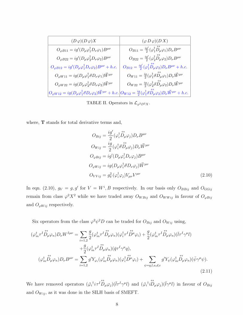
• ϕ2X2

As it was discussed for ϕ2D2X, some of the operators of class ϕ2X2 were traded in favour

of the previous ones. Rest of the operators in this category are listed in Table III.

ϕ2X2

OBB11 = g′2(ϕ†1ϕ1)BµνBµν OGG11 = g2

s(ϕ†1ϕ1)GaµνG

aµν

OBB22 = g′2(ϕ†2ϕ2)BµνBµν OGG22 = g2

s(ϕ†2ϕ2)GaµνG

aµν

OBB12 = g′2(ϕ†1ϕ2 + h.c.)BµνBµν OGG12 = g2

s(ϕ†1ϕ2 + h.c.)GaµνG

aµν

TABLE III. Operators in Lϕ2X2 .

• ϕ6

These are the corrections to the potential of the renormalizable 2HDM and are listed in

Appendix C along with the modified minimisation conditions of the potential.

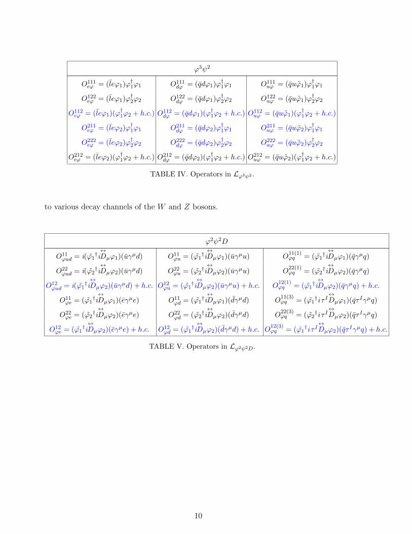
• ϕ3ψ2

These operators lead to the corrections to the Yukawa terms. It is worth noting that we

have written all the possible operators without considering any Z2 charges of either the scalar

doublets or the SM fermions. While working in a particular case of either Type I, II, X or Y

2HDM, certain operators of this category have to be put to zero depending on the discrete

charges of the scalars and fermions. All the operators of this category are listed in Table IV.

• ϕ2ψ2D

Some operators of this category were traded away in favour of some ϕ2D2X type of operators

using eqn. (2.11). The remaining operators are listed in Table V. These operators contribute

9

ϕ3ψ2

O111eϕ = (leϕ1)ϕ†1ϕ1 O111

dϕ = (qdϕ1)ϕ†1ϕ1 O111uϕ = (quϕ1)ϕ†1ϕ1

O122eϕ = (leϕ1)ϕ†2ϕ2 O122


O112eϕ = (leϕ1)(ϕ†1ϕ2 + h.c.) O112

dϕ = (qdϕ1)(ϕ†1ϕ2 + h.c.) O112uϕ = (quϕ1)(ϕ†1ϕ2 + h.c.)

O211eϕ = (leϕ2)ϕ†1ϕ1 O211


O222eϕ = (leϕ2)ϕ†2ϕ2 O222


O212eϕ = (leϕ2)(ϕ†1ϕ2 + h.c.) O212

dϕ = (qdϕ2)(ϕ†1ϕ2 + h.c.) O212uϕ = (quϕ2)(ϕ†1ϕ2 + h.c.)

TABLE IV. Operators in Lϕ3ψ2 .

to various decay channels of the W and Z bosons.

ϕ2ψ2D

O11ϕud = i(ϕ1

†i↔Dµϕ1)(uγµd) O11

ϕu = (ϕ1†i↔Dµϕ1)(uγµu) O

11(1)ϕq = (ϕ1

†i↔Dµϕ1)(qγµq)

O22ϕud = i(ϕ2

†i↔Dµϕ2)(uγµd) O22

ϕu = (ϕ2†i↔Dµϕ2)(uγµu) O

22(1)ϕq = (ϕ2

†i↔Dµϕ2)(qγµq)

O12ϕud = i(ϕ1

†i↔Dµϕ2)(uγµd) + h.c. O12

ϕu = (ϕ1†i↔Dµϕ2)(uγµu) + h.c. O

12(1)ϕq = (ϕ1

†i↔Dµϕ2)(qγµq) + h.c.

O11ϕe = (ϕ1

†i↔Dµϕ1)(eγµe) O11

ϕd = (ϕ1†i↔Dµϕ1)(dγµd) O

11(3)ϕq = (ϕ1

†i τ I↔Dµϕ1)(qτ Iγµq)

O22ϕe = (ϕ2

†i↔Dµϕ2)(eγµe) O22

ϕd = (ϕ2†i↔Dµϕ2)(dγµd) O

22(3)ϕq = (ϕ2

†i τ I↔Dµϕ2)(qτ Iγµq)

O12ϕe = (ϕ1

†i↔Dµϕ2)(eγµe) + h.c. O12

ϕd = (ϕ1†i↔Dµϕ2)(dγµd) + h.c. O

12(3)ϕq = (ϕ1

†i τ I↔Dµϕ2)(qτ Iγµq) + h.c.

TABLE V. Operators in Lϕ2ψ2D.

10

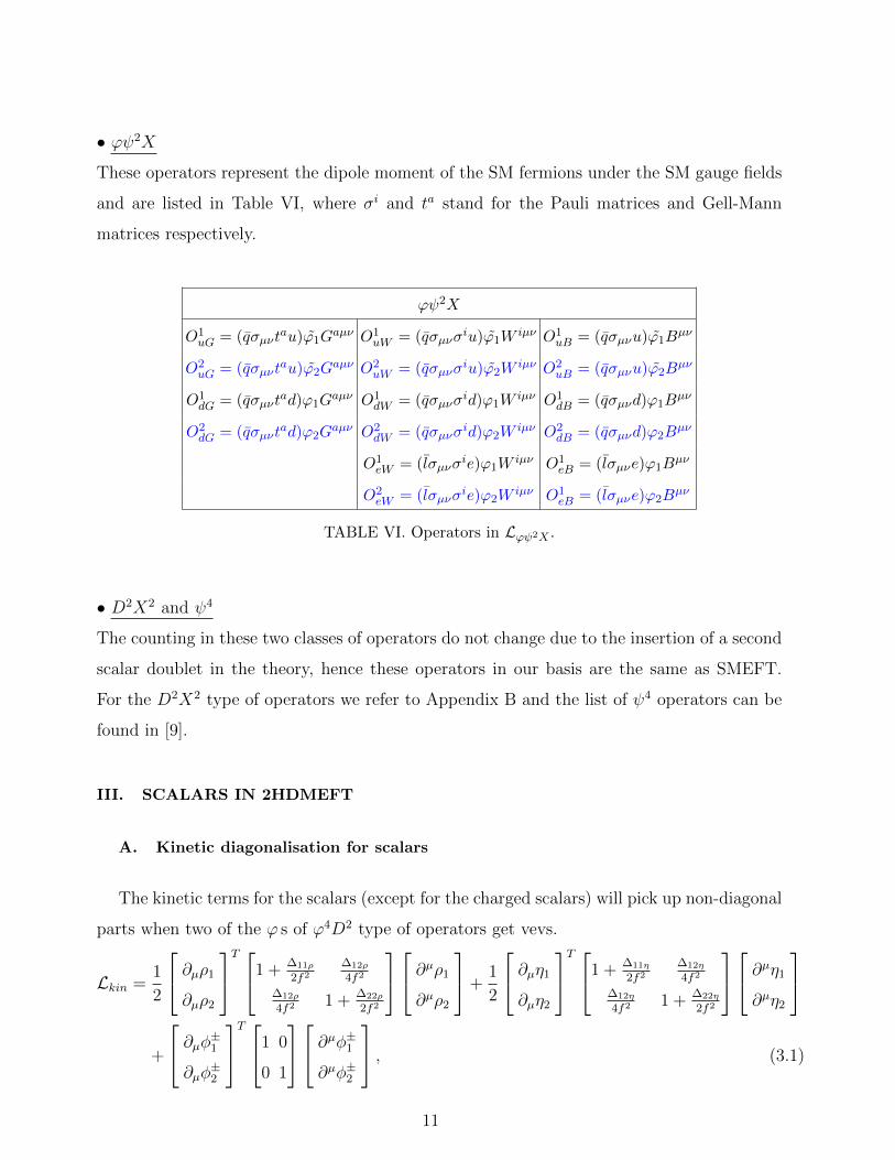
• ϕψ2X

These operators represent the dipole moment of the SM fermions under the SM gauge fields

and are listed in Table VI, where σi and ta stand for the Pauli matrices and Gell-Mann

matrices respectively.

ϕψ2X

O1uG = (qσµνt

au)ϕ1Gaµν O1

uW = (qσµνσiu)ϕ1W

iµν O1uB = (qσµνu)ϕ1B

µν

O2uG = (qσµνt

au)ϕ2Gaµν O2

uW = (qσµνσiu)ϕ2W

iµν O2uB = (qσµνu)ϕ2B

µν

O1dG = (qσµνt

ad)ϕ1Gaµν O1

dW = (qσµνσid)ϕ1W

iµν O1dB = (qσµνd)ϕ1B

µν

O2dG = (qσµνt

ad)ϕ2Gaµν O2

dW = (qσµνσid)ϕ2W

iµν O2dB = (qσµνd)ϕ2B

µν

O1eW = (lσµνσ

ie)ϕ1Wiµν O1

eB = (lσµνe)ϕ1Bµν

O2eW = (lσµνσ

ie)ϕ2Wiµν O1

eB = (lσµνe)ϕ2Bµν

TABLE VI. Operators in Lϕψ2X .

• D2X2 and ψ4

The counting in these two classes of operators do not change due to the insertion of a second

scalar doublet in the theory, hence these operators in our basis are the same as SMEFT.

For the D2X2 type of operators we refer to Appendix B and the list of ψ4 operators can be

found in [9].

III. SCALARS IN 2HDMEFT

A. Kinetic diagonalisation for scalars

The kinetic terms for the scalars (except for the charged scalars) will pick up non-diagonal

parts when two of the ϕ s of ϕ4D2 type of operators get vevs.

Lkin =1

2

∂µρ1

∂µρ2

T 1 + ∆11ρ

2f2∆12ρ

4f2

∆12ρ

4f21 + ∆22ρ

2f2

∂µρ1

∂µρ2

+1

2

∂µη1

∂µη2

T 1 + ∆11η

2f2∆12η

4f2

∆12η

4f21 + ∆22η

2f2

∂µη1

∂µη2

+

∂µφ±1∂µφ

±2

T 1 0

0 1

∂µφ±1∂µφ±2

, (3.1)

11

where,

∆11ρ = 4cH1v21 +

(4cH12 + 2cT3 + c(1)22(1)

)v2

2 + 4cH1H12v1v2,

∆22ρ =(

4cH12 + 2cT3 + c(2)11(2)

)v2

1 + 4cH2v22 + 4cH2H12v1v2,

∆12ρ = 2cH1H12v21 + 2cH2H12v

22 +

(4cH12 + 2cH1H2 − 2cT3 + c(1)21(2) + c(1)12(2)

)v1v2,

∆11η = −4cT1v21 +

(c(1)22(1) − 2cT3

)v2

2 − 4cT4v1v2,

∆22η =(c(2)11(2) − 2cT3

)v2

1 − 4cT2v22 − 4cT5v1v2,

∆12η = −4cT4v21 − 4cT5v

22 +

(c(1)12(2) − 2cT3 − c(1)21(2)

)v1v2. (3.2)

One has to shift the fields in order to diagonalise the kinetic terms in the following manner:

ρ1 → ρ1

(1− ∆11ρ

4f 2

)− ρ2

∆12ρ

8f 2,

ρ2 → ρ2

(1− ∆22ρ

4f 2

)− ρ1

∆12ρ

8f 2,

η1 → η1

(1− ∆11η

4f 2

)− η2

∆12η

8f 2,

η2 → η2

(1− ∆22η

4f 2

)− η1

∆12η

8f 2,

φ±1,2 → φ±1,2. (3.3)

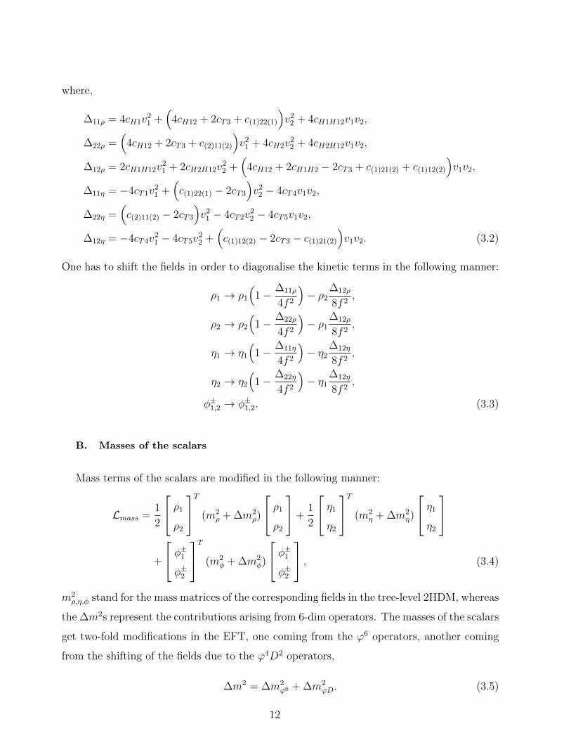
B. Masses of the scalars

Mass terms of the scalars are modified in the following manner:

Lmass =1

2

ρ1

ρ2

T (m2ρ + ∆m2

ρ)

ρ1

ρ2

+1

2

η1

η2

T (m2η + ∆m2

η)

η1

η2

+

φ±1φ±2

T (m2φ + ∆m2

φ)

φ±1φ±2

, (3.4)

m2ρ,η,φ stand for the mass matrices of the corresponding fields in the tree-level 2HDM, whereas

the ∆m2s represent the contributions arising from 6-dim operators. The masses of the scalars

get two-fold modifications in the EFT, one coming from the ϕ6 operators, another coming

from the shifting of the fields due to the ϕ4D2 operators,

∆m2 = ∆m2ϕ6 + ∆m2

ϕD. (3.5)

12

m2η + ∆m2

ηϕ6 =(m2

12 −1

2(2λ5v1v2 + λ6v

21 + λ7v

22) +

C1

f 2

)tan β −1

−1 cot β

,m2φ + ∆m2

φϕ6 =(m2

12 −1

2((λ4 + λ5)v1v2 + λ6v

21 + λ7v

22) +

C2

f 2

)tan β −1

−1 cot β

,(3.6)

where,

C1 = −[v1v2(v2

1c(1212)1 + v22c(1212)2)

+v21v

22

(1

4c(1221)12 +

1

4c12(12) + 3c121212

)+v4

1

4c11(12) +

v42

4c22(12)

],

C2 = −[v1v2

2

(v2

1(c(1212)1 +1

2c(1221)1) + v2

2(c(1212)2 +1

2c(1221)2)

)+v2

1v22

(3

4c(1221)12 +

1

4c12(12) + 3c121212

)+v4

1

4c11(12) +

v42

4c22(12)

]. (3.7)

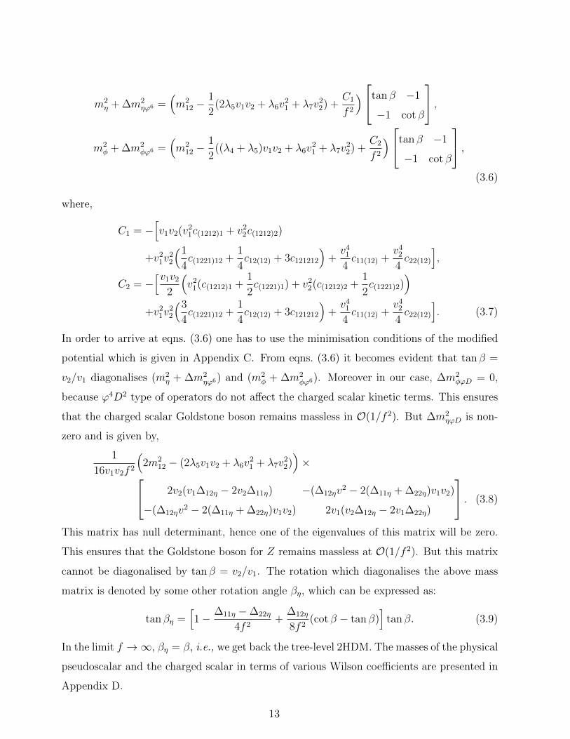
In order to arrive at eqns. (3.6) one has to use the minimisation conditions of the modified

potential which is given in Appendix C. From eqns. (3.6) it becomes evident that tan β =

v2/v1 diagonalises (m2η + ∆m2

ηϕ6) and (m2φ + ∆m2

φϕ6). Moreover in our case, ∆m2φϕD = 0,

because ϕ4D2 type of operators do not affect the charged scalar kinetic terms. This ensures

that the charged scalar Goldstone boson remains massless in O(1/f 2). But ∆m2ηϕD is non-

zero and is given by,

1

16v1v2f 2

(2m2

12 − (2λ5v1v2 + λ6v21 + λ7v

22))× 2v2(v1∆12η − 2v2∆11η) −(∆12ηv

2 − 2(∆11η + ∆22η)v1v2)

−(∆12ηv2 − 2(∆11η + ∆22η)v1v2) 2v1(v2∆12η − 2v1∆22η)

. (3.8)

This matrix has null determinant, hence one of the eigenvalues of this matrix will be zero.

This ensures that the Goldstone boson for Z remains massless at O(1/f 2). But this matrix

cannot be diagonalised by tan β = v2/v1. The rotation which diagonalises the above mass

matrix is denoted by some other rotation angle βη, which can be expressed as:

tan βη =[1− ∆11η −∆22η

4f 2+

∆12η

8f 2(cot β − tan β)

]tan β. (3.9)

In the limit f →∞, βη = β, i.e., we get back the tree-level 2HDM. The masses of the physical

pseudoscalar and the charged scalar in terms of various Wilson coefficients are presented in

Appendix D.

13

In a similar manner, ∆m2ρϕ6 and ∆m2

ρϕD will both have non-zero values and the rotation

needed for diagonalising ∆m2ρ will no longer be the same as α in 2HDM at the tree-level.

We call the new rotation angle α′. The value of α′ can be determined from the masses of

the neutral scalars after fixing the values of relevant Wilson coefficients. If the light and the

heavy scalars have masses mh and mH respectively [33],

sinα′ =M2

12ρ√(M2

12ρ)2 + (M2

11ρ −m2h)

2,

m2H =

M211ρ(M2

11ρ −m2h) + (M2

12ρ)2

(M211ρ −m2

h). (3.10)

The expressions for M211ρ and M2

12ρ in our case are given in Appendix D.

IV. CONSTRAINTS FROM ELECTROWEAK PRECISION OBSERVABLES

We consider all the bosonic classes, i.e., ϕ4D2, ϕ6, ϕ2D2X, ϕ2X2, and see which ones are

constrained by EWPT. Some of the operators of class ϕ4D2 contribute to the T parameter

and are constrained at per-mille level. But the rest of the operators of class ϕ4D2 can only

be constrained by demanding perturbative unitarity [26]. The operators of class ϕ6 do not

contribute to the precision observables at all, though they can be constrained by demanding

perturbative unitarity. The operators of class ϕ2D2X are constrained at per-mille level by

the precision tests, in particular, by the measurement of S parameter and the anomalous

triple gauge boson vertices (TGV) which we will discuss shortly. The operators of class ϕ2X2

do not contribute to the precision observables.

The operators of class D2X2 in our basis are the same as the ones in SMEFT, as they

include no Higgs doublets. Operators of type D2X2 contribute to the oblique parameters

V , W , Y and Z and can be constrained from measurements at LEP. We shall mention the

bounds for completeness.

We have not considered the EWPT constraints on the fermionic operator classes, i.e.,

ϕ3ψ2, ϕ2ψ2D, ϕψ2X and ψ4. However, we mention that the operators of class ϕ2ψ2D can

be constrained using the EWPT because they lead to various fermionic decay channels of

W and Z bosons. The operators of type ψ4 in our basis are the same as in SMEFT. These

operators are bounded by the measurements of muon lifetime, four-fermion scatterings in

14

LEP and LHC, etc. Operators of type ϕ3ψ2 and ϕψ2X do not contribute to the precision

observables. In this paper, we have considered only the tree-level effects of the operators of

our basis on the precision observables.

In a SILH scenario, the coupling of the new dynamics is stronger compared to the SM

ones, i.e., gSM � gρ . 4π [5]. This prescription distinguishes the mass of lightest vector

resonance of the strong sector mρ ∼ gρf from its cut-off Λ ∼ 4πf . To show quantitatively

what value gρ can attain in a realistic scenario, in SO(6)/SO(4) × SO(2) composite Higgs

model with the third generation quark doublet and tR, both transforming as 4 of SO(4) [14],

one finds that gρ ∼ 3.6 < 4π for mh ∼ 125 GeV. In the remaining part of this paper, we will

use the SILH suppressions of the Wilson coefficients for different classes of operators. We

have used the shorthand notation of ξi, where i = 1, .., 5, to describe these suppressions and

these are defined in Appendix B. All the bounds we impose on the Wilson coefficients from

now on, can be translated to a non-SILH scenario in the limit ξi → 1/f 2, f being the scale

of new physics.

• Constraints from anomalous TGVs

TGVs [34] involving W bosons are some of the precisely measured quantities in the

LEP experiment. Anomalous contribution to TGVs can be parametrised in terms of five

parameters which are defined in Appendix E. The operators from class ϕ2D2X, except

OBij, contribute to these parameters in the following way:

δg1Z =

1

cos2 θw

[(cϕW11 c

2β + cϕW22 s

2β + 2 cϕW12 sβ cβ)ξ2

+(cW11 c2β + cW22 s

2β + 2cW12 sβ cβ)ξ1

]m2W ,

δκγ =[(cϕB11 + cϕW11) c2

β + (cϕB22 + cϕW22) s2β + 2 (cϕB12 + cϕW12) sβ cβ

]m2W ξ2,

δκZ = δg1Z − tan2 θwδκγ, λγ = λZ = 0. (4.1)

We use the bounds from two parameter fit (δg1Z and δκγ) with λγ = 0 of anomalous TGVs

at 95% confidence level provided by LEP-II collaboration [35]:

−4.6× 10−2 6 δg1Z 6 5.0× 10−2,

−1.1× 10−1 6 δκγ 6 8.4× 10−2. (4.2)

15

It is worth mentioning here that, λγ and λZ get affected by the CP-odd operator WµνWµρW ν

ρ .

As we are considering only the CP-even operators in this paper, λγ = λZ = 0 in our basis.

Inclusion of the Higgs signal strength data in the fit changes the bounds on anomalous

TGVs. The fitted values of δg1Z and δκγ at 95% confidence level [36] become:

−1.9× 10−2 6 δg1Z 6 7.2× 10−3,

−2.8× 10−2 6 δκγ 6 0.312. (4.3)

The 6-dim operators in our basis also contribute to the Higgs signal strengths. So, in order

to extract the bounds on the Wilson coefficients using eqn. (4.3), extra care has to be taken.

• Constraints from oblique parameters

We define vacuum polarisation amplitude involving any two vector bosons VI and VJ as

ΠµνIJ(p) = ΠIJ(p2)gµν−∆(p2)pµpν , where ΠIJ(p2) = [ΠIJ(0)+p2Π′IJ(0)+p4Π′′IJ(0)+ ...]. The

6-dim operators in our basis modify these polarisation amplitudes. Ward identity requires

that Πγγ(0) = ΠγZ(0) = 0, which we have verified. The oblique parameters S, T , U , V , W ,

Y and Z, are expressed as different combinations of the polarisation amplitudes and their

derivatives [31, 37, 38]. Among these, only S, T and U can be measured using the Z-pole

observables. The kinetic terms of W±µ and Bµ must be normalised before calculating the

oblique parameters [31]. Due to the presence of the ϕ2X2 type of operators, the kinetic term

of Bµ has to be canonically normalised with help of following transformation:

Bµ →(

1 + g′2v2ξ3(cBB11c2β + cBB22s

2β + 2cBB12sβcβ)

)Bµ. (4.4)

However, such transformation need not be done for W±µ as the corresponding operators do

not exist in our basis, as it can be seen in Table III.

The contribution of the effective operators to oblique parameter U is zero. As, U ∝

(Π′W+W−(0) − Π′33(0)), non-zero value of U demands a source of isospin-violation in the

theory. In our basis, these two polarisation amplitudes get modified by the operators OWij,

but in an identical way, giving U = 0.

16

However, the other two parameters S and T get non-zero contributions in our basis:

S =16πv2

m2ρ

[(cW11 + cB11)c2

β + (cW22 + cB22)s2β + 2(cW12 + cB12)sβcβ

],

T =1

α

v2

f 2

(cT1c

4β + cT2s

4β + 2cT s

2βc

2β + 2cT4c

3βsβ + 2cT5s

3βcβ

), (4.5)

where,

cT = cT3 −1

8(c(1)22(1) + c(2)11(2))−

1

4(c(1)21(2) + c(1)12(2)). (4.6)

As it was mentioned earlier, it can be seen that the operators that contribute to S and

T belong to the classes ϕ2D2X and ϕ4D2 respectively. Bounds at 95% confidence limit on

S and T are given by [39]:

S ∈ [−0.12, 0.15], T ∈ [−0.04, 0.24].

The oblique parameters V , W , Y and Z can not be measured using the Z-pole observables.

They represent second derivatives of certain polarisation amplitudes. D2X2 type of operators

affect the oblique parameters V , W , Y and Z in following manner [5]:

V = Π′′W+W−(0)− Π′′33(0) = 0,

W = Π′′33(0) = c2Wg2m2

W ξ4,

Y = Π′′BB(0) = c2Bg′2m2

W ξ4,

Z = Π′′GG(0) = c2Gg2sm

2W ξ4, (4.7)

whereas the LEP data suggests [31]:

−4.7× 10−3 6 W 6 0.7× 10−3,

−0.7× 10−3 6 Y 6 8.9× 10−3. (4.8)

V = 0 for the same reason as why U = 0, i.e., there is no source of isospin-violation. The

parameter Z could not be constrained from LEP because it is insensitive to the measurements

of the electroweak sector.

One can find out the changes in the values of the precision observables due to the inclusion

of any kind of new physics from its contributions to the oblique parameters etc. [40]. For

example, the change in mW and sin2 θw in terms of S, T , U can be written as:

mW = mZ

∣∣SM

(0.881− (2.80× 10−3)S + (4.31× 10−3)T + (3.25× 10−3)U

),

sin2∗ θ(m

2Z) = 0.23149 + (3.64× 10−3)S − (2.59× 10−3)T. (4.9)

17

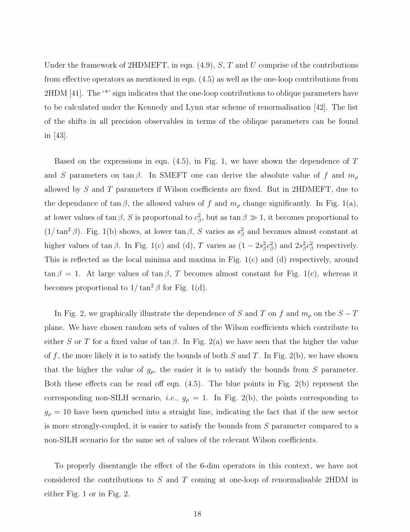
Under the framework of 2HDMEFT, in eqn. (4.9), S, T and U comprise of the contributions

from effective operators as mentioned in eqn. (4.5) as well as the one-loop contributions from

2HDM [41]. The ‘*’ sign indicates that the one-loop contributions to oblique parameters have

to be calculated under the Kennedy and Lynn star scheme of renormalisation [42]. The list

of the shifts in all precision observables in terms of the oblique parameters can be found

in [43].

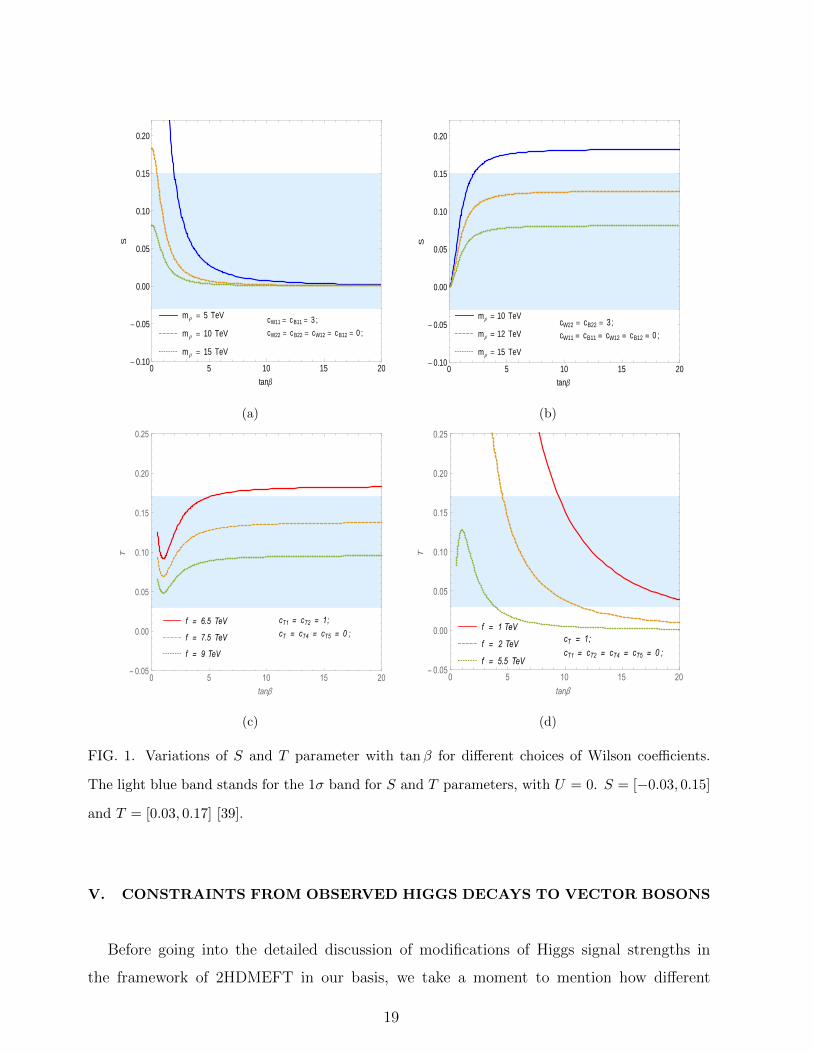
Based on the expressions in eqn. (4.5), in Fig. 1, we have shown the dependence of T

and S parameters on tan β. In SMEFT one can derive the absolute value of f and mρ

allowed by S and T parameters if Wilson coefficients are fixed. But in 2HDMEFT, due to

the dependance of tan β, the allowed values of f and mρ change significantly. In Fig. 1(a),

at lower values of tan β, S is proportonal to c2β, but as tan β � 1, it becomes proportional to

(1/ tan2 β). Fig. 1(b) shows, at lower tan β, S varies as s2β and becomes almost constant at

higher values of tan β. In Fig. 1(c) and (d), T varies as (1 − 2s2βc

2β) and 2s2

βc2β respectively.

This is reflected as the local minima and maxima in Fig. 1(c) and (d) respectively, around

tan β = 1. At large values of tan β, T becomes almost constant for Fig. 1(c), whereas it

becomes proportional to 1/ tan2 β for Fig. 1(d).

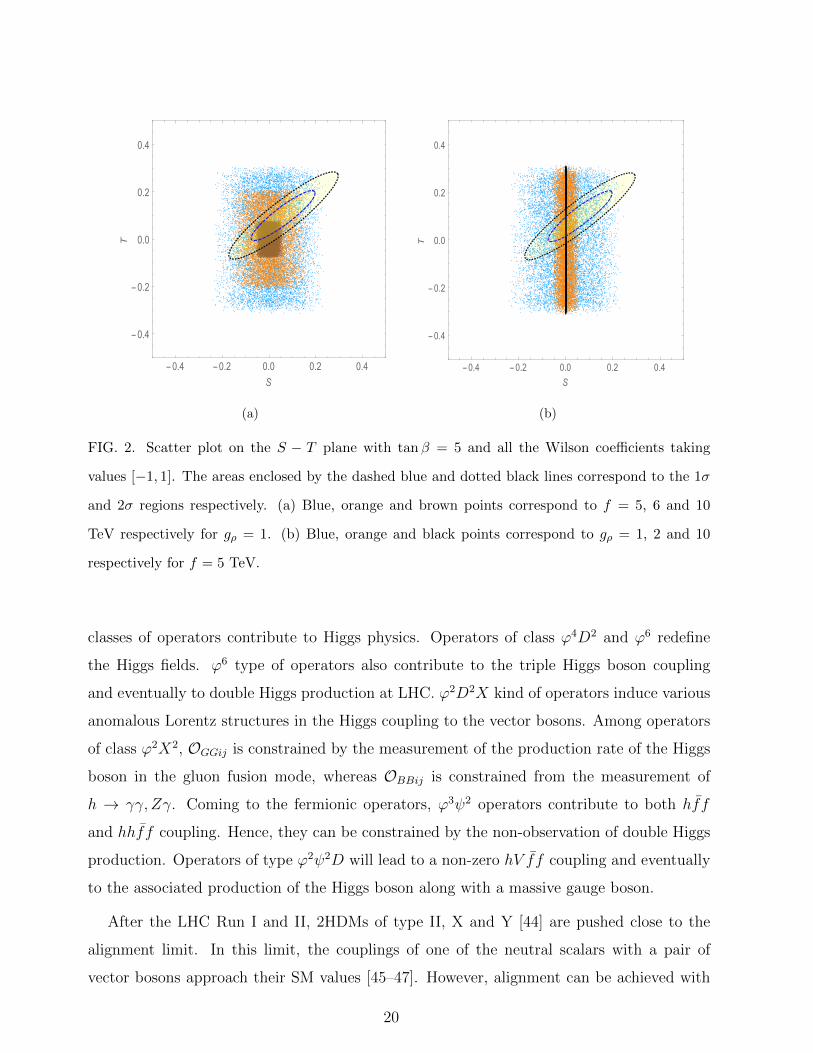
In Fig. 2, we graphically illustrate the dependence of S and T on f and mρ on the S − T

plane. We have chosen random sets of values of the Wilson coefficients which contribute to

either S or T for a fixed value of tan β. In Fig. 2(a) we have seen that the higher the value

of f , the more likely it is to satisfy the bounds of both S and T . In Fig. 2(b), we have shown

that the higher the value of gρ, the easier it is to satisfy the bounds from S parameter.

Both these effects can be read off eqn. (4.5). The blue points in Fig. 2(b) represent the

corresponding non-SILH scenario, i.e., gρ = 1. In Fig. 2(b), the points corresponding to

gρ = 10 have been quenched into a straight line, indicating the fact that if the new sector

is more strongly-coupled, it is easier to satisfy the bounds from S parameter compared to a

non-SILH scenario for the same set of values of the relevant Wilson coefficients.

To properly disentangle the effect of the 6-dim operators in this context, we have not

considered the contributions to S and T coming at one-loop of renormalisable 2HDM in

either Fig. 1 or in Fig. 2.

18

m Ρ = 5 TeV

m Ρ = 10 TeV

m Ρ = 15 TeV

cW11 = cB11 = 3 ;

cW22 = cB22 = cW12 = cB12 = 0 ;

0 5 10 15 20- 0.10

- 0.05

0.00

0.05

0.10

0.15

0.20

tanΒ

S

(a)

m Ρ = 10 TeV

m Ρ = 12 TeV

m Ρ = 15 TeV

cW22 = cB22 = 3 ;cW11 = cB11 = cW12 = cB12 = 0 ;

0 5 10 15 20- 0.10

- 0.05

0.00

0.05

0.10

0.15

0.20

tanΒ

S(b)

f = 6.5 TeV

f = 7.5 TeV

f = 9 TeV

cT1 = cT2 = 1;

cT = cT4 = cT5 = 0 ;

0 5 10 15 20- 0.05

0.00

0.05

0.10

0.15

0.20

0.25

tanβ

T

(c)

f = 1 TeV

f = 2 TeV

f = 5.5 TeV

cT = 1;

cT1 = cT2 = cT4 = cT5 = 0 ;

0 5 10 15 20- 0.05

0.00

0.05

0.10

0.15

0.20

0.25

tanβ

T

(d)

FIG. 1. Variations of S and T parameter with tanβ for different choices of Wilson coefficients.

The light blue band stands for the 1σ band for S and T parameters, with U = 0. S = [−0.03, 0.15]

and T = [0.03, 0.17] [39].

V. CONSTRAINTS FROM OBSERVED HIGGS DECAYS TO VECTOR BOSONS

Before going into the detailed discussion of modifications of Higgs signal strengths in

the framework of 2HDMEFT in our basis, we take a moment to mention how different

19

-0.4 -0.2 0.0 0.2 0.4

-0.4

-0.2

0.0

0.2

0.4

S

T

(a)

-0.4 -0.2 0.0 0.2 0.4

-0.4

-0.2

0.0

0.2

0.4

S

T(b)

FIG. 2. Scatter plot on the S − T plane with tanβ = 5 and all the Wilson coefficients taking

values [−1, 1]. The areas enclosed by the dashed blue and dotted black lines correspond to the 1σ

and 2σ regions respectively. (a) Blue, orange and brown points correspond to f = 5, 6 and 10

TeV respectively for gρ = 1. (b) Blue, orange and black points correspond to gρ = 1, 2 and 10

respectively for f = 5 TeV.

classes of operators contribute to Higgs physics. Operators of class ϕ4D2 and ϕ6 redefine

the Higgs fields. ϕ6 type of operators also contribute to the triple Higgs boson coupling

and eventually to double Higgs production at LHC. ϕ2D2X kind of operators induce various

anomalous Lorentz structures in the Higgs coupling to the vector bosons. Among operators

of class ϕ2X2, OGGij is constrained by the measurement of the production rate of the Higgs

boson in the gluon fusion mode, whereas OBBij is constrained from the measurement of

h → γγ, Zγ. Coming to the fermionic operators, ϕ3ψ2 operators contribute to both hff

and hhff coupling. Hence, they can be constrained by the non-observation of double Higgs

production. Operators of type ϕ2ψ2D will lead to a non-zero hV ff coupling and eventually

to the associated production of the Higgs boson along with a massive gauge boson.

After the LHC Run I and II, 2HDMs of type II, X and Y [44] are pushed close to the

alignment limit. In this limit, the couplings of one of the neutral scalars with a pair of

vector bosons approach their SM values [45–47]. However, alignment can be achieved with

20

or without Appelquist-Carazzone decoupling [48] of the new scalars. We are interested in

the scenario of ‘alignment without decoupling’ [33, 49, 50].

As the decay into γγ, Zγ and gg channels are loop mediated processes in renormalisable

2HDM, there will be interferences of the one loop amplitudes with the ones coming due to

higher dimensional operators. The modified matrix elements are given by:

|A|2 ' |A′ 2HDM |2 + 2Re[A2HDM∗ ×∆A], (5.1)

where, A2HDM is the one-loop amplitude for the relevant process in 2HDM. A′ 2HDM is

the amplitude of the corresponding process consisting of contributions from one-loop of

2HDM and the 6-dim operators of type ϕ4D2, ϕ6 and ϕ3ψ2 whose effects are not studied

here numerically. ∆A is the contribution coming from operators O(W,B,ϕW,ϕB,ϕ2X2)ij. In

eqn. (5.1), we have neglected the effects which are quadratic in the Wilson coefficients, i.e.,

O((∆A)2)→ 0 and (A′ 2HDM∗∆A)→ (A2HDM∗∆A). After parametrising the effects of the

6-dim operators as:

L ⊃(cγγ

2FµνF

µν + cZγZµνFµν +

cgg2GµνG

µν)hv, (5.2)

one obtains the partial decay width of SM-like Higgs to γγ and Zγ with help of the

eqn. (5.1) [51],

Γ(h→ γγ)∣∣EFT' GFα

2emm

3h

128√

2π3

[ ∣∣A′ 2HDM(γγ)∣∣2 + 2Re

[ 4π

αemcγγ A2HDM∗(γγ)

]],

Γ(h→ Zγ)∣∣EFT' G2

Fαemm2Wm

3h

64π4

(1− m2

Z

m2h

)3[∣∣A′ 2HDM(Zγ)∣∣2

+2Re[− 4π√αemα2

cZγA2HDM∗(Zγ)]]. (5.3)

21

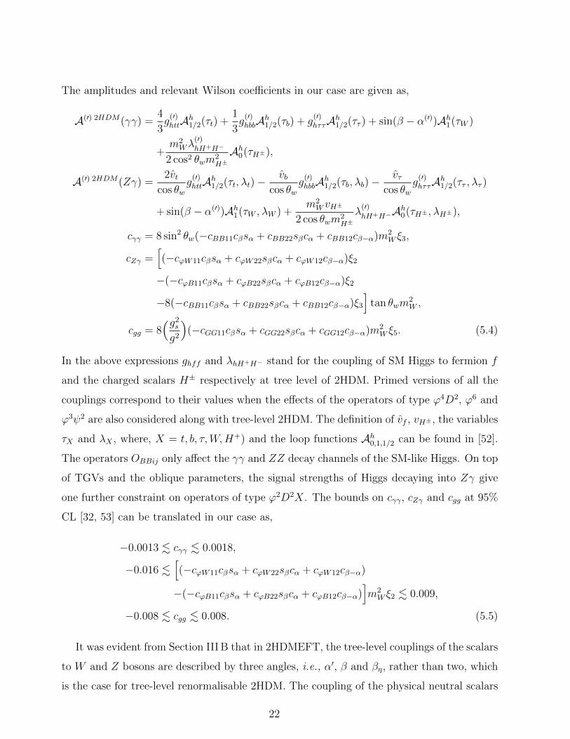
The amplitudes and relevant Wilson coefficients in our case are given as,

A(′) 2HDM(γγ) =4

3g

(′)httA

h1/2(τt) +

1

3g

(′)hbbA

h1/2(τb) + g

(′)hττA

h1/2(ττ ) + sin(β − α(′))Ah1(τW )

+m2Wλ

(′)hH+H−

2 cos2 θwm2H±Ah0(τH±),

A(′) 2HDM(Zγ) =2vt

cos θwg

(′)httA

h1/2(τt, λt)−

vbcos θw

g(′)hbbA

h1/2(τb, λb)−

vτcos θw

g(′)hττA

h1/2(ττ , λτ )

+ sin(β − α(′))Ah1(τW , λW ) +m2WvH±

2 cos θwm2H±

λ(′)hH+H−A

h0(τH± , λH±),

cγγ = 8 sin2 θw(−cBB11cβsα + cBB22sβcα + cBB12cβ−α)m2W ξ3,

cZγ =[(−cϕW11cβsα + cϕW22sβcα + cϕW12cβ−α)ξ2

−(−cϕB11cβsα + cϕB22sβcα + cϕB12cβ−α)ξ2

−8(−cBB11cβsα + cBB22sβcα + cBB12cβ−α)ξ3

]tan θwm

2W ,

cgg = 8(g2

s

g2

)(−cGG11cβsα + cGG22sβcα + cGG12cβ−α)m2

W ξ5. (5.4)

In the above expressions ghff and λhH+H− stand for the coupling of SM Higgs to fermion f

and the charged scalars H± respectively at tree level of 2HDM. Primed versions of all the

couplings correspond to their values when the effects of the operators of type ϕ4D2, ϕ6 and

ϕ3ψ2 are also considered along with tree-level 2HDM. The definition of vf , vH± , the variables

τX and λX , where, X = t, b, τ,W,H+) and the loop functions Ah0,1,1/2 can be found in [52].

The operators OBBij only affect the γγ and ZZ decay channels of the SM-like Higgs. On top

of TGVs and the oblique parameters, the signal strengths of Higgs decaying into Zγ give

one further constraint on operators of type ϕ2D2X. The bounds on cγγ, cZγ and cgg at 95%

CL [32, 53] can be translated in our case as,

−0.0013 . cγγ . 0.0018,

−0.016 .[(−cϕW11cβsα + cϕW22sβcα + cϕW12cβ−α)

−(−cϕB11cβsα + cϕB22sβcα + cϕB12cβ−α)]m2W ξ2 . 0.009,

−0.008 . cgg . 0.008. (5.5)

It was evident from Section III B that in 2HDMEFT, the tree-level couplings of the scalars

to W and Z bosons are described by three angles, i.e., α′, β and βη, rather than two, which

is the case for tree-level renormalisable 2HDM. The coupling of the physical neutral scalars

22

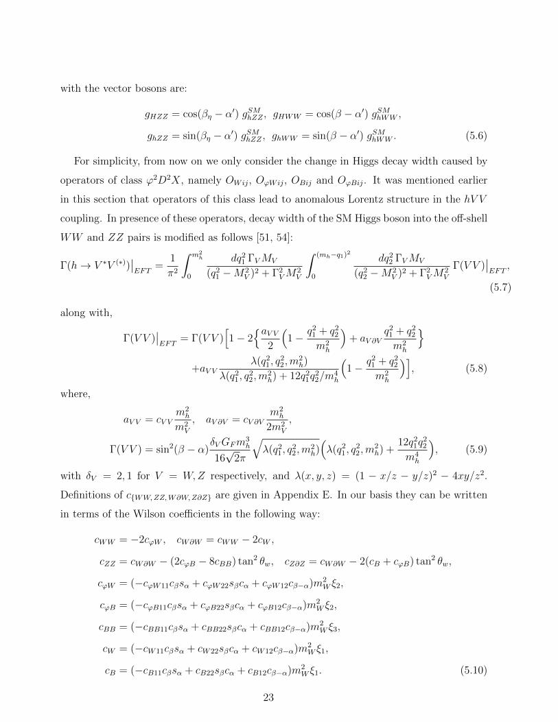
with the vector bosons are:

gHZZ = cos(βη − α′) gSMhZZ , gHWW = cos(β − α′) gSMhWW ,

ghZZ = sin(βη − α′) gSMhZZ , ghWW = sin(β − α′) gSMhWW . (5.6)

For simplicity, from now on we only consider the change in Higgs decay width caused by

operators of class ϕ2D2X, namely OWij, OϕWij, OBij and OϕBij. It was mentioned earlier

in this section that operators of this class lead to anomalous Lorentz structure in the hV V

coupling. In presence of these operators, decay width of the SM Higgs boson into the off-shell

WW and ZZ pairs is modified as follows [51, 54]:

Γ(h→ V ∗V (∗))∣∣EFT

=1

π2

∫ m2h

0

dq21 ΓVMV

(q21 −M2

V )2 + Γ2VM

2V

∫ (mh−q1)2

0

dq22 ΓVMV

(q22 −M2

V )2 + Γ2VM

2V

Γ(V V )∣∣EFT

,

(5.7)

along with,

Γ(V V )∣∣EFT

= Γ(V V )[1− 2

{aV V2

(1− q2

1 + q22

m2h

)+ aV ∂V

q21 + q2

2

m2h

}+aV V

λ(q21, q

22,m

2h)

λ(q21, q

22,m

2h) + 12q2

1q22/m

4h

(1− q2

1 + q22

m2h

)], (5.8)

where,

aV V = cV Vm2h

m2V

, aV ∂V = cV ∂Vm2h

2m2V

,

Γ(V V ) = sin2(β − α)δVGFm

3h

16√

2π

√λ(q2

1, q22,m

2h)(λ(q2

1, q22,m

2h) +

12q21q

22

m4h

), (5.9)

with δV = 2, 1 for V = W,Z respectively, and λ(x, y, z) = (1 − x/z − y/z)2 − 4xy/z2.

Definitions of c{WW,ZZ,W∂W,Z∂Z} are given in Appendix E. In our basis they can be written

in terms of the Wilson coefficients in the following way:

cWW = −2cϕW , cW∂W = cWW − 2cW ,

cZZ = cW∂W − (2cϕB − 8cBB) tan2 θw, cZ∂Z = cW∂W − 2(cB + cϕB) tan2 θw,

cϕW = (−cϕW11cβsα + cϕW22sβcα + cϕW12cβ−α)m2W ξ2,

cϕB = (−cϕB11cβsα + cϕB22sβcα + cϕB12cβ−α)m2W ξ2,

cBB = (−cBB11cβsα + cBB22sβcα + cBB12cβ−α)m2W ξ3,

cW = (−cW11cβsα + cW22sβcα + cW12cβ−α)m2W ξ1,

cB = (−cB11cβsα + cB22sβcα + cB12cβ−α)m2W ξ1. (5.10)

23

One can see in eqn. (5.10), all the Wilson coefficients are constrained by either S parameter

in eqn. (4.5) or anomalous TGVs eqn. (4.1) or the measurement of decay width of Higgs to

γγ and Zγ in eqn. (5.5). This happens in SMEFT as well. But these Wilson coefficients

appeared with prefactors different from those in eqns. (4.1) and (4.5). This is a remarkable

feature of 2HDMEFT. For example, the Wilson coefficient of OW11 has come with a prefactor

of c2β and −cβsα in the expressions for S parameter and hWW coupling respectively, and

would come with a prefactor of s2α in the hhWW coupling. This effect is absent in SMEFT.

The following numerical analysis will illustrate this fact.

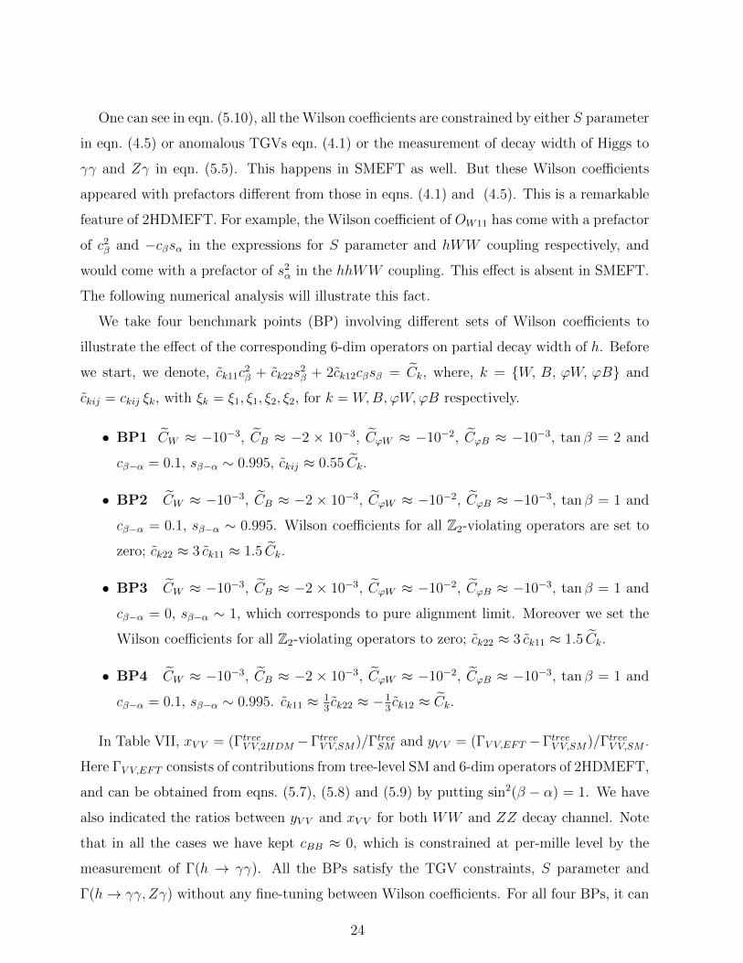
We take four benchmark points (BP) involving different sets of Wilson coefficients to

illustrate the effect of the corresponding 6-dim operators on partial decay width of h. Before

we start, we denote, ck11c2β + ck22s

2β + 2ck12cβsβ = Ck, where, k = {W, B, ϕW, ϕB} and

ckij = ckij ξk, with ξk = ξ1, ξ1, ξ2, ξ2, for k = W,B,ϕW,ϕB respectively.

• BP1 CW ≈ −10−3, CB ≈ −2 × 10−3, CϕW ≈ −10−2, CϕB ≈ −10−3, tan β = 2 and

cβ−α = 0.1, sβ−α ∼ 0.995, ckij ≈ 0.55 Ck.


cβ−α = 0.1, sβ−α ∼ 0.995. Wilson coefficients for all Z2-violating operators are set to

zero; ck22 ≈ 3 ck11 ≈ 1.5 Ck.


cβ−α = 0, sβ−α ∼ 1, which corresponds to pure alignment limit. Moreover we set the

Wilson coefficients for all Z2-violating operators to zero; ck22 ≈ 3 ck11 ≈ 1.5 Ck.


cβ−α = 0.1, sβ−α ∼ 0.995. ck11 ≈ 13ck22 ≈ −1

3ck12 ≈ Ck.

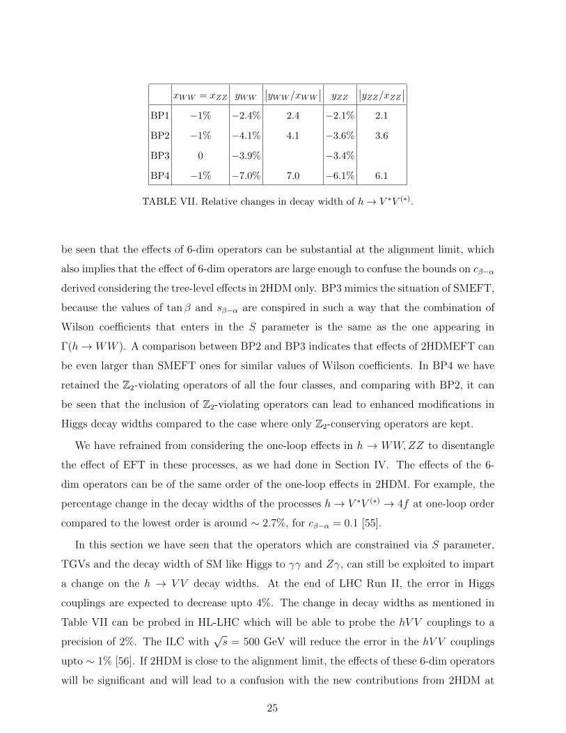
In Table VII, xV V = (ΓtreeV V,2HDM −ΓtreeV V,SM)/ΓtreeSM and yV V = (ΓV V,EFT −ΓtreeV V,SM)/ΓtreeV V,SM .

Here ΓV V,EFT consists of contributions from tree-level SM and 6-dim operators of 2HDMEFT,

and can be obtained from eqns. (5.7), (5.8) and (5.9) by putting sin2(β − α) = 1. We have

also indicated the ratios between yV V and xV V for both WW and ZZ decay channel. Note

that in all the cases we have kept cBB ≈ 0, which is constrained at per-mille level by the

measurement of Γ(h → γγ). All the BPs satisfy the TGV constraints, S parameter and

Γ(h→ γγ, Zγ) without any fine-tuning between Wilson coefficients. For all four BPs, it can

24

xWW = xZZ yWW

∣∣yWW /xWW

∣∣ yZZ∣∣yZZ/xZZ∣∣

BP1 −1% −2.4% 2.4 −2.1% 2.1

BP2 −1% −4.1% 4.1 −3.6% 3.6

BP3 0 −3.9% −3.4%

BP4 −1% −7.0% 7.0 −6.1% 6.1

TABLE VII. Relative changes in decay width of h→ V ∗V (∗).

be seen that the effects of 6-dim operators can be substantial at the alignment limit, which

also implies that the effect of 6-dim operators are large enough to confuse the bounds on cβ−α

derived considering the tree-level effects in 2HDM only. BP3 mimics the situation of SMEFT,

because the values of tan β and sβ−α are conspired in such a way that the combination of

Wilson coefficients that enters in the S parameter is the same as the one appearing in

Γ(h→ WW ). A comparison between BP2 and BP3 indicates that effects of 2HDMEFT can

be even larger than SMEFT ones for similar values of Wilson coefficients. In BP4 we have

retained the Z2-violating operators of all the four classes, and comparing with BP2, it can

be seen that the inclusion of Z2-violating operators can lead to enhanced modifications in

Higgs decay widths compared to the case where only Z2-conserving operators are kept.

We have refrained from considering the one-loop effects in h → WW,ZZ to disentangle

the effect of EFT in these processes, as we had done in Section IV. The effects of the 6-

dim operators can be of the same order of the one-loop effects in 2HDM. For example, the

percentage change in the decay widths of the processes h→ V ∗V (∗) → 4f at one-loop order

compared to the lowest order is around ∼ 2.7%, for cβ−α = 0.1 [55].

In this section we have seen that the operators which are constrained via S parameter,

TGVs and the decay width of SM like Higgs to γγ and Zγ, can still be exploited to impart

a change on the h → V V decay widths. At the end of LHC Run II, the error in Higgs

couplings are expected to decrease upto 4%. The change in decay widths as mentioned in

Table VII can be probed in HL-LHC which will be able to probe the hV V couplings to a

precision of 2%. The ILC with√s = 500 GeV will reduce the error in the hV V couplings

upto ∼ 1% [56]. If 2HDM is close to the alignment limit, the effects of these 6-dim operators

will be significant and will lead to a confusion with the new contributions from 2HDM at

25

tree and loop level effects for the respective processes.

VI. DISCUSSIONS

Non-observation of any beyond standard model particle in the direct searches at LHC

motivates us to adhere to the language of effective field theory. 2HDM is a viable extension

of the scalar sector of the SM. The main motivation for considering a 2HDMEFT comes

from the fact that observations of a SM-like Higgs boson has pushed 2HDM to be at the

alignment limit if the new scalars are at a sub-TeV scale. In such a scenario, the new

scalars get almost decoupled at the vertices with SM particles that include a gauge boson.

As a result, deviations of the contribution of four-dimensional Lagrangian of 2HDM to SM

processes are small compared to its SM counterpart. We have shown that contributions of

the six-dimensional operators of 2HDMEFT are comparable with the deviation due to tree

level contributions in 2HDM at the alignment limit from SM. Such effects can interfere in

determination of 2HDM parameter space from experiments.

In this work, we have presented a complete basis for six-dimensional operators in 2HDM

motivated by the SILH [5] in SMEFT. Such an extension is not trivial and demands careful

use of EoMs to eliminate redundant operators. For simplicity, we have restricted ourselves

to CP- and flavour-conserving ones. Due to various reasons, as mentioned in the text, in

SMEFT, the SILH basis is often favoured for Higgs physics studies. Hence, we feel that our

basis would be useful for the community practising 2HDM phenomenology.

In presence of a strongly interacting weak sector just beyond a TeV or so, which we

designate in this paper as ‘SILH scenario’, the hierarchy problem in Higgs mass reduces

to a ‘Little’ hierarchy problem, thereby alleviating the quadratic divergences. The 2HDM

can originate from such an underlying strong dynamics. In this case, one need not bother

about hard Z2-violating terms and hence, we include them all, even in the six-dimensional

Lagrangian. In a SILH scenario the Wilson coefficients of the operators come with various

suppression factors which we review in Appendix A. In passing, we emphasize that our basis

has a wider applicability – it is valid when such a SILH scenario is envisaged or not.

Next, we have let the operators confront the results from the electroweak precision tests

and measured values of Higgs production and decay channels concentrating only on bosonic

26

operators of classes ϕ4D2, ϕ6, ϕ2D2X and ϕ2X2 containing the new scalars. Ensuing bounds

on combinations of Wilson coefficients have been extracted. Out of these classes, some of the

operators belonging only to the classes ϕ4D2 and ϕ2D2X were constrained from EWPT. The

operators of class ϕ6 and some of the operators of class ϕ4D2 can be constrained demanding

perturbative unitarity. As expected, constraints from EWPT are much tighter than those

from considerations of unitarity. We also consider the class D2X2 which contribute to W ,

Y and Z parameters in EWPT. For completeness, we have mentioned bounds on these as

well, but these are the same as in SMEFT. In discussing impacts on Higgs signal strengths,

only the operators of the class ϕ2D2X and ϕ2X2 have been considered for simplicity. As

the phenomenology of 2HDMEFT is quite rich, to avoid cluttering of information we have

also avoided considering phenomenology of the fermionic operators of classes ϕ3ψ2, ϕ2ψ2D,

ϕψ2X and ψ4. These issues will be addressed elsewhere.

An earlier attempt to present a basis of Z2-conserving operators for 2HDMEFT was made

in Ref. [27] that resembles the Warsaw basis in SMEFT. But we have found one redundant

operator in the class ϕ4D2. In our basis, kinetic mixing of the gauge eigenstates of the scalar

were taken care of by field redefinitions and their effect on determining the masses of the

physical scalar were also calculated. An important feature of our basis is that the charged

scalar mass matrix is still diagonalised by tan β = v2/v1 as in the tree-level 2HDM. But

the neutral psuedoscalar sector needs a diagonalisation matrix which is not characterised by

the same tan β. So the kinetic diagonalisation changes the pseudoscalar mass matrix, but

not the one for the charged scalars. This is reflected in the expressions for masses of the

pseudoscalar and the charged scalars that we have presented in Appendix D.

An interesting feature of 2HDMEFT is that, in contrast to SMEFT, here the 2HDM

parameter space plays a crucial role while placing bounds on the Wilson coefficients. For

example, the same Wilson coefficient can appear with different prefactors in the expressions

for precision parameters and for Higgs decay widths. These prefactors depend on the 2HDM

parameter space. This happens because unlike SM, in 2HDM the interaction eigenstates of

the scalars are not the same as their mass eigenstates. In Section V we have numerically

demonstrated this remarkable effect which is absent in SMEFT.

In short, our complete basis of 2HDMEFT will facilitate further studies of 2HDM phe-

nomenology. We have presented constraints on some of the operators and pointed out that

27

such constraints do depend on the 2HDM parameter space. Such dependence can signifi-

cantly modify some of the predictions of SMEFT. It was also noticed that, in the vicinity

of the alignment limit, the effects of the higher dimensional operators in determining the

parameter space of 2HDM are not negligible.

VII. ACKNOWLEDGEMENTS

S.K. thanks A. Falkowski for email communications. S.R. is supported by the Department

of Science and Technology, India via Grant No. EMR/2014/001177.

28

Appendix A: Rules for dimensional analysis

If the BSM strong sector is characterized by mass-scale mρ compared to mW for SM, the

effective operators induced by the former will be made of local operators made out of SM

fields and derivatives [57, 58]:

LEFT =m4ρ

g2ρ

L(Dµ

mρ

,gρϕ

mρ

,gρfL,R

m3/2ρ

,gSMX

m2ρ

)ϕ, fL,R and X stand for the scalars, fermions and field strengths of SM gauge fields respec-

tively. The above relation can be described by putting ~ 6= 1 and counting the dimension of

all SM fields and gρ in powers of ~. One finds that, [gρ] = ~−1/2, [ϕ] = [Vµ] = [M ]~1/2 etc.

The naive dimensional counting rules for the Wilson coefficients of operators in SILH basis,

as were introduced in [5], are based on above expansion,

(I) A factor of 1/f for an extra Goldstone leg;

(II) A factor of 1/mρ for an extra derivative, i.e., 1/m2ρ for an extra X;

(III) A suppression of 1/m2ρ along with an extra SM vector boson field strength.

Extra suppressions in an SILH scenario are as follows: ϕ4D2, ϕ6, ϕ2ψ2D and ϕ3ψ2 are

suppressed by 1/f 2, following rule (I). ϕ2X2, ϕ2D2X and ϕψ2X should have been suppressed

by 1/m2ρ, using rule (II). But the operators of type OϕW and OϕB can not be generated at the

tree level by integrating out a new resonance and thus come with a suppression of 1/(4πf)2.

Physical Higgs is neutral under SU(3)C × U(1)em. So, the gauging of these groups do not

break the shift symmetry of physical pNGB Higgs. On the other hand, operators of type

ϕ2X2 generate the coupling of physical Higgs with a pair of on-shell photons and gluons,

for X = B,G respectively and also break the shift symmetry. The latter fact is reflected

in an extra suppression of (gSM/gρ)2 for the ϕ2X2 type of operators. Moreover, operator

of type ϕ3ψ2 get an extra suppression of the Yukawa coupling yψ. In the similar manner,

in our basis of 2HDMEFT, operators of type (leϕi)(ϕ†jϕk), (qdϕi)(ϕ

†jϕk) and (quϕi)(ϕ

†jϕk)

from Table IV get suppressed by Y ei , Y d

i and Y ui respectively.

The SILH basis of 6-dim operators in SMEFT with their corresponding suppressions are

given in Appendix B.

29

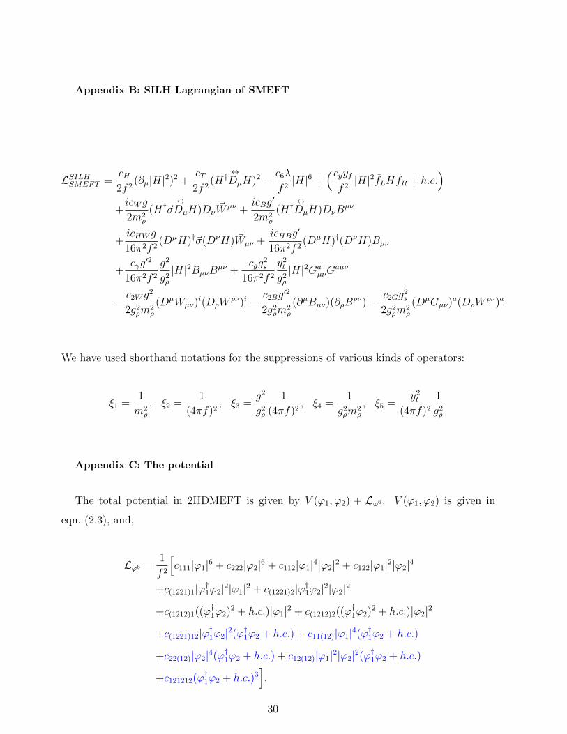
Appendix B: SILH Lagrangian of SMEFT

LSILHSMEFT =cH2f 2

(∂µ|H|2)2 +cT2f 2

(H†↔DµH)2 − c6λ

f 2|H|6 +

(cyyff 2|H|2fLHfR + h.c.

)+icWg

2m2ρ

(H†~σ↔DµH)Dν

~W µν +icBg

′

2m2ρ

(H†↔DµH)DνB

µν

+icHWg

16π2f 2(DµH)†~σ(DνH) ~Wµν +

icHBg′

16π2f 2(DµH)†(DνH)Bµν

+cγg′2

16π2f 2

g2

g2ρ

|H|2BµνBµν +

cgg2s

16π2f 2

y2t

g2ρ

|H|2GaµνG

aµν

− c2Wg2

2g2ρm

2ρ

(DµWµν)i(DρW

ρν)i − c2Bg′2

2g2ρm

2ρ

(∂µBµν)(∂ρBρν)− c2Gg

2s

2g2ρm

2ρ

(DµGµν)a(DρW

ρν)a.

We have used shorthand notations for the suppressions of various kinds of operators:

ξ1 =1

m2ρ

, ξ2 =1

(4πf)2, ξ3 =

g2

g2ρ

1

(4πf)2, ξ4 =

1

g2ρm

2ρ

, ξ5 =y2t

(4πf)2

1

g2ρ

.

Appendix C: The potential

The total potential in 2HDMEFT is given by V (ϕ1, ϕ2) + Lϕ6 . V (ϕ1, ϕ2) is given in

eqn. (2.3), and,

Lϕ6 =1

f 2

[c111|ϕ1|6 + c222|ϕ2|6 + c112|ϕ1|4|ϕ2|2 + c122|ϕ1|2|ϕ2|4

+c(1221)1|ϕ†1ϕ2|2|ϕ1|2 + c(1221)2|ϕ†1ϕ2|2|ϕ2|2

+c(1212)1((ϕ†1ϕ2)2 + h.c.)|ϕ1|2 + c(1212)2((ϕ†1ϕ2)2 + h.c.)|ϕ2|2

+c(1221)12|ϕ†1ϕ2|2(ϕ†1ϕ2 + h.c.) + c11(12)|ϕ1|4(ϕ†1ϕ2 + h.c.)

+c22(12)|ϕ2|4(ϕ†1ϕ2 + h.c.) + c12(12)|ϕ1|2|ϕ2|2(ϕ†1ϕ2 + h.c.)

+c121212(ϕ†1ϕ2 + h.c.)3].

30

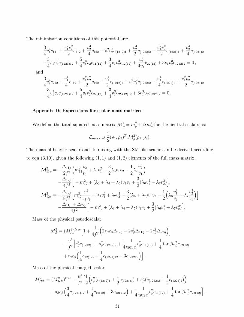
The minimisation conditions of this potential are:

3

4v4

1c111 +v2

1v22

2c112 +

v42

4c122 + v2

1v22c(1212)1 +

v42

2c(1212)2 +

v21v

22

2c(1221)1 +

v42

4c(1221)2

+3

4v1v

32c(1221)12 +

5

4v3

1v2c11(12) +3

4v1v

32c12(12) +

v52

4v1

c22(12) + 3v1v32c121212 = 0 ,

and

3

4v4

2c222 +v4

1

4c112 +

v21v

22

2c122 +

v41

2c(1212)1 + v2

1v22c(1212)2 +

v41

4c(1221)1 +

v21v

22

2c(1221)2

+3

4v3

1v2c(1221)12 +5

4v1v

32c22(12) +

3

4v3

1v2c(12)12 + 3v31v2c121212 = 0 .

Appendix D: Expressions for scalar mass matrices

We define the total squared mass matrix M2ρ = m2

ρ + ∆m2ρ for the neutral scalars as:

Lmass ⊃1

2(ρ1, ρ2)TM2

ρ(ρ1, ρ2).

The mass of heavier scalar and its mixing with the SM-like scalar can be derived according

to eqn (3.10), given the following (1, 1) and (1, 2) elements of the full mass matrix,

M211ρ = −∆11ρ

2f 2

(m2

12

v2

v1

+ λ1v21 +

3

2λ6v1v2 −

1

2λ7v3

2

v1

)−∆12ρ

4f 2

[−m2

12 + (λ3 + λ4 + λ5)v1v2 +3

2(λ6v

21 + λ7v

22)],

M212ρ = −∆12ρ

8f 2

[m2

12

v2

v1v2

+ λ1v21 + λ2v

22 +

3

2(λ6 + λ7)v1v2 −

1

2

(λ6v3

1

v2

+ λ7v3

2

v1

)]−∆11ρ + ∆22ρ

4f 2

[−m2

12 + (λ3 + λ4 + λ5)v1v2 +3

2(λ6v

21 + λ7v

22)].

Mass of the physical psuedoscalar,

M2A = (M2

A)tree[1 +

1

4f 2

(2sβcβ∆12η − 2s2

β∆11η − 2c2β∆22η

)]−v

4

f 2

[c2βc(1212)1 + s2

βc(1212)2 +1

4

1

tan βc2βc11(12) +

1

4tan βs2

βc22(12)

+sβcβ

(1

4c12(12) +

1

4c(1221)12 + 3c121212

)].

Mass of the physical charged scalar,

M2H± = (M2

H±)tree − v4

f 2

[1

2

(c2β(c(1212)1 +

1

2c(1221)1) + s2

β(c(1212)2 +1

2c(1221)2)

)+sβcβ

(3

4c(1221)12 +

1

4c12(12) + 3c121212

)+

1

4

1

tan βc2βc11(12) +

1

4tan βs2

βc22(12)

].

31

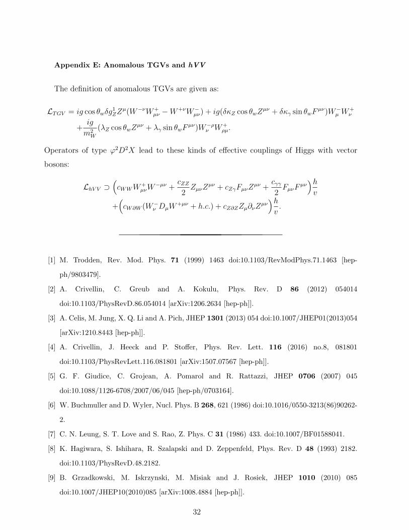
Appendix E: Anomalous TGVs and hVV

The definition of anomalous TGVs are given as:

LTGV = ig cos θwδg1ZZ

µ(W−νW+µν −W+νW−

µν) + ig(δκZ cos θwZµν + δκγ sin θwF

µν)W−µ W

+ν

+ig

m2W

(λZ cos θwZµν + λγ sin θwF

µν)W−ρν W+

ρµ.

Operators of type ϕ2D2X lead to these kinds of effective couplings of Higgs with vector

bosons:

LhV V ⊃(cWWW

+µνW

−µν +cZZ2ZµνZ

µν + cZγFµνZµν +

cγγ2FµνF

µν)hv

+(cW∂W (W−

ν DµW+µν + h.c.) + cZ∂ZZµ∂νZ

µν)hv.

[1] M. Trodden, Rev. Mod. Phys. 71 (1999) 1463 doi:10.1103/RevModPhys.71.1463 [hep-

ph/9803479].

[2] A. Crivellin, C. Greub and A. Kokulu, Phys. Rev. D 86 (2012) 054014

doi:10.1103/PhysRevD.86.054014 [arXiv:1206.2634 [hep-ph]].

[3] A. Celis, M. Jung, X. Q. Li and A. Pich, JHEP 1301 (2013) 054 doi:10.1007/JHEP01(2013)054

[arXiv:1210.8443 [hep-ph]].

[4] A. Crivellin, J. Heeck and P. Stoffer, Phys. Rev. Lett. 116 (2016) no.8, 081801

doi:10.1103/PhysRevLett.116.081801 [arXiv:1507.07567 [hep-ph]].

[5] G. F. Giudice, C. Grojean, A. Pomarol and R. Rattazzi, JHEP 0706 (2007) 045

doi:10.1088/1126-6708/2007/06/045 [hep-ph/0703164].

[6] W. Buchmuller and D. Wyler, Nucl. Phys. B 268, 621 (1986) doi:10.1016/0550-3213(86)90262-

2.

[7] C. N. Leung, S. T. Love and S. Rao, Z. Phys. C 31 (1986) 433. doi:10.1007/BF01588041.

[8] K. Hagiwara, S. Ishihara, R. Szalapski and D. Zeppenfeld, Phys. Rev. D 48 (1993) 2182.

doi:10.1103/PhysRevD.48.2182.

[9] B. Grzadkowski, M. Iskrzynski, M. Misiak and J. Rosiek, JHEP 1010 (2010) 085

doi:10.1007/JHEP10(2010)085 [arXiv:1008.4884 [hep-ph]].

32

[10] K. Agashe, R. Contino and A. Pomarol, Nucl. Phys. B 719, 165 (2005)

doi:10.1016/j.nuclphysb.2005.04.035 [hep-ph/0412089].

[11] N. Arkani-Hamed, A. G. Cohen, E. Katz and A. E. Nelson, JHEP 0207 (2002) 034

doi:10.1088/1126-6708/2002/07/034 [hep-ph/0206021].

[12] A. Falkowski, Pramana 87 (2016) no.3, 39 doi:10.1007/s12043-016-1251-5 [arXiv:1505.00046

[hep-ph]].

[13] I. Brivio and M. Trott, arXiv:1706.08945 [hep-ph].

[14] J. Mrazek, A. Pomarol, R. Rattazzi, M. Redi, J. Serra and A. Wulzer, Nucl. Phys. B 853, 1

(2011) doi:10.1016/j.nuclphysb.2011.07.008 [arXiv:1105.5403 [hep-ph]].

[15] S. De Curtis, S. Moretti, K. Yagyu and E. Yildirim, Phys. Rev. D 94 (2016) no.5, 055017


[16] S. De Curtis, S. Moretti, K. Yagyu and E. Yildirim, arXiv:1612.05125 [hep-ph].

[17] S. De Curtis, S. Moretti, K. Yagyu and E. Yildirim, arXiv:1702.07260 [hep-ph].

[18] T. Brown, C. Frugiuele and T. Gregoire, JHEP 1106 (2011) 108 doi:10.1007/JHEP06(2011)108

[arXiv:1012.2060 [hep-ph]].

[19] S. Gopalakrishna, T. S. Mukherjee and S. Sadhukhan, Phys. Rev. D 94 (2016) no.1, 015034


[20] N. Fonseca, R. Zukanovich Funchal, A. Lessa and L. Lopez-Honorez, JHEP 1506 (2015) 154


[21] A. Carmona and M. Chala, JHEP 1506 (2015) 105 doi:10.1007/JHEP06(2015)105

[arXiv:1504.00332 [hep-ph]].

[22] M. Chala, G. Durieux, C. Grojean, L. de Lima and O. Matsedonskyi, arXiv:1703.10624 [hep-

ph].

[23] J. L. Diaz-Cruz, J. Hernandez-Sanchez and J. J. Toscano, Phys. Lett. B 512 (2001) 339

doi:10.1016/S0370-2693(01)00703-1 [hep-ph/0106001].

[24] Y. Kikuta and Y. Yamamoto, Eur. Phys. J. C 76 (2016) no.5, 297 doi:10.1140/epjc/s10052-

016-4128-3 [arXiv:1510.05540 [hep-ph]].

[25] Y. Kikuta, Y. Okada and Y. Yamamoto, Phys. Rev. D 85 (2012) 075021


33

[26] Y. Kikuta and Y. Yamamoto, PTEP 2013 (2013) 053B05 doi:10.1093/ptep/ptt030

[arXiv:1210.5674 [hep-ph]].

[27] A. Crivellin, M. Ghezzi and M. Procura, JHEP 1609 (2016) 160 doi:10.1007/JHEP09(2016)160

[arXiv:1608.00975 [hep-ph]].

[28] I. F. Ginzburg and M. Krawczyk, Phys. Rev. D 72 (2005) 115013

doi:10.1103/PhysRevD.72.115013 [hep-ph/0408011].

[29] I. F. Ginzburg, Phys. Lett. B 682 (2009) 61 doi:10.1016/j.physletb.2009.10.071

[arXiv:0810.1546 [hep-ph]].

[30] H. D. Politzer, Nucl. Phys. B 172 (1980) 349 doi:10.1016/0550-3213(80)90172-8.

[31] R. Barbieri, A. Pomarol, R. Rattazzi and A. Strumia, Nucl. Phys. B 703 (2004) 127

doi:10.1016/j.nuclphysb.2004.10.014 [hep-ph/0405040].

[32] J. Elias-Miro, J. R. Espinosa, E. Masso and A. Pomarol, JHEP 1311, 066 (2013)


[33] M. Carena, I. Low, N. R. Shah and C. E. M. Wagner, JHEP 1404 (2014) 015


[34] K. Hagiwara, R. D. Peccei, D. Zeppenfeld and K. Hikasa, Nucl. Phys. B 282 (1987) 253

doi:10.1016/0550-3213(87)90685-7.

[35] The LEP collaborations ALEPH, DELPHI, L3, OPAL, and the LEP TGC Working Group,

LEPEWWG/TGC/2003-01.

[36] A. Falkowski, M. Gonzalez-Alonso, A. Greljo and D. Marzocca, Phys. Rev. Lett. 116 (2016)

no.1, 011801 doi:10.1103/PhysRevLett.116.011801 [arXiv:1508.00581 [hep-ph]].

[37] I. Maksymyk, C. P. Burgess and D. London, Phys. Rev. D 50 (1994) 529


[38] M. E. Peskin and T. Takeuchi, Phys. Rev. D 46 (1992) 381 doi:10.1103/PhysRevD.46.381.

[39] M. Baak et al. [Gfitter Group], Eur. Phys. J. C 74 (2014) 3046 doi:10.1140/epjc/s10052-014-

3046-5 [arXiv:1407.3792 [hep-ph]].

[40] C. P. Burgess, S. Godfrey, H. Konig, D. London and I. Maksymyk, Phys. Rev. D 49 (1994)

6115 doi:10.1103/PhysRevD.49.6115 [hep-ph/9312291].

[41] H. E. Haber and D. O’Neil, Phys. Rev. D 83 (2011) 055017 doi:10.1103/PhysRevD.83.055017

[arXiv:1011.6188 [hep-ph]].

34

[42] D. C. Kennedy and B. W. Lynn, Nucl. Phys. B 322 (1989) 1. doi:10.1016/0550-3213(89)90483-

5.

[43] C. P. Burgess, Pramana 45 (1995) S47 doi:10.1007/BF02907965 [hep-ph/9411257].

[44] M. Aoki, S. Kanemura, K. Tsumura and K. Yagyu, Phys. Rev. D 80 (2009) 015017


[45] O. Eberhardt, U. Nierste and M. Wiebusch, JHEP 1307 (2013) 118


[46] H. E. Haber and O. Stal, Eur. Phys. J. C 75 (2015) no.10, 491 Erratum: [Eur. Phys. J.

C 76 (2016) no.6, 312] doi:10.1140/epjc/s10052-015-3697-x, 10.1140/epjc/s10052-016-4151-4

[arXiv:1507.04281 [hep-ph]].

[47] H. Blusca-Mato, A. Falkowski, D. Fontes, J. C. Romo and J. P. Silva, Eur. Phys. J. C 77

(2017) no.3, 176 doi:10.1140/epjc/s10052-017-4745-5 [arXiv:1611.01112 [hep-ph]].

[48] T. Appelquist and J. Carazzone, Phys. Rev. D 11 (1975) 2856. doi:10.1103/PhysRevD.11.2856.

[49] J. F. Gunion and H. E. Haber, Phys. Rev. D 67 (2003) 075019


[50] P. S. Bhupal Dev and A. Pilaftsis, JHEP 1412 (2014) 024 Erratum: [JHEP 1511 (2015) 147]

doi:10.1007/JHEP11(2015)147, 10.1007/JHEP12(2014)024 [arXiv:1408.3405 [hep-ph]].

[51] R. Contino, M. Ghezzi, C. Grojean, M. Muhlleitner and M. Spira, JHEP 1307 (2013) 035


[52] A. Djouadi, Phys. Rept. 459 (2008) 1 doi:10.1016/j.physrep.2007.10.005 [hep-ph/0503173].

[53] A. Falkowski, F. Riva and A. Urbano, JHEP 1311 (2013) 111 doi:10.1007/JHEP11(2013)111

[arXiv:1303.1812 [hep-ph]].

[54] R. N. Cahn, Rept. Prog. Phys. 52 (1989) 389. doi:10.1088/0034-4885/52/4/001.

[55] L. Altenkamp, S. Dittmaier and H. Rzehak, arXiv:1704.02645 [hep-ph].

[56] S. Dawson et al., arXiv:1310.8361 [hep-ex].

[57] M. A. Luty, Phys. Rev. D 57 (1998) 1531 doi:10.1103/PhysRevD.57.1531 [hep-ph/9706235].

[58] A. Pomarol, arXiv:1412.4410 [hep-ph].

35

Documents

Siddhartha Karmakar and Subhendu Rakshity - arXiv · Higher dimensional operators in 2HDM Siddhartha Karmakar and Subhendu Rakshity Discipline of Physics, Indian Institute of Technology