SIAM J. COMPUT cˆ—Received by the editors April 12, 2002; accepted for publication (in revised form) March 27, 2004; published electronically October 1, 2004. A preliminary version

FAST UNIVERSALIZATION OF INVESTMENT STRATEGIES∗

KARHAN AKCOGLU† , PETROS DRINEAS‡ , AND MING-YANG KAO§

SIAM J. COMPUT. c© 2004 Society for Industrial and Applied MathematicsVol. 34, No. 1, pp. 1–22

Abstract. A universalization of a parameterized investment strategy is an online algorithmwhose average daily performance approaches that of the strategy operating with the optimal param-eters determined offline in hindsight. We present a general framework for universalizing investmentstrategies and discuss conditions under which investment strategies are universalizable. We presentexamples of common investment strategies that fit into our framework. The examples include bothtrading strategies that decide positions in individual stocks, and portfolio strategies that allocatewealth among multiple stocks. This work extends in a natural way Cover’s universal portfolio work.We also discuss the runtime efficiency of universalization algorithms. While a straightforward im-plementation of our algorithms runs in time exponential in the number of parameters, we show thatthe efficient universal portfolio computation technique of Kalai and Vempala [Proceedings of the41st Annual IEEE Symposium on Foundations of Computer Science, Redondo Beach, CA, 2000,pp. 486–491] involving the sampling of log-concave functions can be generalized to other classes ofinvestment strategies, thus yielding provably good approximation algorithms in our framework.

Key words. universal portfolios, computational finance, portfolio optimization, investmentstrategies, portfolio strategies, trading strategies, constantly rebalanced portfolios

AMS subject classifications. 91B28, 68Q32, 68W40

DOI. 10.1137/S0097539702405619

1. Introduction. An age-old question in finance deals with how to managemoney on the stock market to obtain an “acceptable” return on investment. Aninvestment strategy is an online algorithm that attempts to address this questionby applying a given set of rules to determine how to invest capital. Typically, aninvestment strategy is parameterized by a vector w ∈ R

∗ =⋃∞

i=1 Ri that dictates how

the strategy operates. The optimal parameters that maximize the strategy’s returnare unknown when the algorithm is run, and the parameters are usually chosen quitearbitrarily. A universalization of an investment strategy is an online algorithm basedon the strategy whose average daily performance approaches that of the strategyoperating with the optimal parameters determined offline in hindsight.

Consider the constantly rebalanced portfolio (CRP) investment strategy univer-salized by Cover [5] and the subject of several extensions and generalizations [3, 6, 11,14, 16, 20]. The CRP strategy maintains a constant proportion of total wealth in eachstock, where the proportions are dictated by the parameters given to the strategy. In

∗Received by the editors April 12, 2002; accepted for publication (in revised form) March 27, 2004;published electronically October 1, 2004. A preliminary version of this work appeared in LectureNotes in Computer Science 2380: Proceedings of the 29th International Colloquium on Automata,Languages, and Programming, M. Hennessy and P. Widmayer, eds., Springer-Verlag, New York,2002, pp. 888–900.

http://www.siam.org/journals/sicomp/34-1/40561.html†The Goldman Sachs Group, New York, NY 10004 ([email protected]). This work

was done while the author was a graduate student at Yale University and was supported in part byNSF grant CCR-9988376.

‡Department of Computer Science, Rensselaer Polytechnic Institute, Troy, NY 12180 ([email protected]). This work was done while the author was a graduate student at Yale University and wassupported in part by NSF grant CCR-9896165.

§Department of Computer Science, Northwestern University, Evanston, IL 60201 ([email protected]). This author’s work was supported in part by NSF grant CCR-9988376.

1

2 KARHAN AKCOGLU, PETROS DRINEAS, AND MING-YANG KAO

a stock market with m stocks, the parameter space for the CRP strategy is

Wm =

w ∈ [0, 1]m

∣∣ m∑i=1

wi = 1

,

the set of vectors in Rm whose components are between 0 and 1 and add up to 1.

Given a portfolio vector w = (w1, . . . , wm) ∈ Wm, wi tells us the proportion of wealthto invest in stock i for 1 ≤ i ≤ m. At the beginning of each day, the holdings arerebalanced ; i.e., money is taken out of some stocks and put into others, so that thedesired proportions are maintained in each stock. As an example of the robustness ofthe CRP strategy, consider the following market with two stocks [11, 16]. The priceof one stock remains constant, while the other stock doubles and halves in price onalternate days. Investing in a single stock will at most double our money. With aCRP ( 1

2 ,12 ) strategy, however, our wealth will increase exponentially, by a factor of

( 12 · 1 + 1

2 · 2) × ( 12 · 1 + 1

2 · 12 ) = 3

2 × 34 = 9

8 every two days.Cover developed an investment strategy that effectively distributes wealth uni-

formly over all portfolio vectors w ∈ Wm on the first day and executes the CRPstrategy with daily rebalancing according to each w on the (infinitesimally small)proportion of wealth initially allocated to each w. Cover showed that the averagedaily log-performance1 of such a strategy approaches that of the CRP strategy oper-ating with the optimal return-maximizing parameters chosen with hindsight.

This paper generalizes previous results and introduces a framework that allowsuniversalizations of other parameterized investment strategies. As we see in section 2,investment strategies typically fall under two categories: trading strategies operateon a single stock and dictate when to buy and short2 the stock; portfolio strategies,such as CRP, operate on the stock market as a whole and dictate how to allocatewealth among multiple stocks. We present several examples of common trading andportfolio strategies that can be universalized in our framework. We discuss our univer-salization framework in section 3. The proofs of our results are very general, and, aswith previous universal portfolio results, we make no assumptions on the underlyingdistribution of the stock prices; our results are applicable for all sequences of stock re-turns and market conditions. The running times of universalization algorithms are, ingeneral, exponential in the number of parameters used by the underlying investmentstrategy. Kalai and Vempala [14] presented an efficient implementation of the CRPalgorithm that runs in time polynomial in the number of parameters. In section 4, wepresent general conditions on investment strategies under which the universalizationalgorithm can be efficiently implemented. We also give some investment strategiesthat satisfy these conditions. Section 5 concludes with directions for further research.

2. Types of investment strategies. Suppose we would like to distribute ourwealth among m stocks.3 Investment strategies are general classes of rules that dictatehow to invest capital. At time t > 0, a strategy S takes as input an environment vectorEt and a parameter vector w, and returns an investment description St(w) specifyinghow to allocate our capital at time t. The environment vector Et contains historic

1The average daily log-performance is the average of the logarithms of the factors by which ourwealth changes on a daily basis. This notion is discussed further in section 3.1.

2A short position in a stock, discussed in section 2.1, allows us to earn a profit when the stockdeclines in value.

3We use the term “stocks” in order to keep our terminology consistent with previous work, butwe actually mean a broader range of investment instruments, including both long and short positionsin stocks.

FAST UNIVERSALIZATION OF INVESTMENT STRATEGIES 3

market information, including stock price history, trading volumes, etc.; the parametervector w is independent of Et and specifies exactly how the strategy S should operate;the investment description St(w) = (St1(w), . . . , Stm(w)) is a vector specifying theproportion of wealth to put in each stock, where we put a fraction Sti(w) of ourholdings in stock i, for 1 ≤ i ≤ m. For example, CRP is an investment strategy;coupled with a portfolio vector w, it tells us to “rebalance our portfolio on a dailybasis according to w”; its investment description, CRPt(w) = w, is independent ofthe market environment Et.

There are two general types of investment strategies that we focus upon in thispaper. Trading strategies tell us whether we should take a long (bet that the stockprice will rise) or a short (bet that the stock price will fall) position on a given stock.Portfolio strategies tell us how to distribute our wealth among various stocks. Weshould note here that these two classes do not exhaust all investment strategies; thereexist strategies that take both long and short positions in several stocks (as in [21]).Trading strategies are denoted by T , and portfolio strategies are denoted by P . Weuse S to denote either kind of strategy. For k ≥ 2, let

Wk =

w = (w1, . . . , wk) ∈ [0, 1]k

∣∣ k∑i=1

wi = 1

.(2.1)

Remark 1. Wk is a (k−1)-dimensional simplex in Rk. The investment strategies

that we describe below are parameterized by vectors in Wk = Wk ×· · ·×Wk ( times)

for some k ≥ 2 and ≥ 1. We may write w ∈ Wk in the form w = (w1, . . . ,w),

where wι = (wι1, . . . , wιk) for 1 ≤ ι ≤ .

2.1. Trading strategies. Suppose that our market contains a single stock. Wehave m = 2 potential investments: either a long position or a short position in thestock. To take a long position, we buy shares in hopes that the share price will rise.We close a long position by selling the shares. The money we use to buy the sharesis our investment in the long position; the value of the investment is the money weget when we close the position. If we let pt denote the stock price at the beginning ofday t, the value of our investment will change by a factor of xt = pt+1

ptfrom day t to

t + 1.To take a short position, we borrow shares from our broker and sell them on the

market in hopes that the share price will fall. We close a short position by buying theshares back and returning them to our broker. As collateral for the borrowed shares,our broker has a margin requirement : a fraction α of the value of the borrowed sharesmust be deposited in a margin account. Should the price of the security rise sufficiently,the collateral in our margin account will not be enough, and the broker will issue amargin call, requiring us to deposit more collateral. The margin requirement is ourinvestment in the short position; the value of the investment is the money we getwhen we close the position.

Lemma 2.1. Let the margin requirement for a short position be α ∈ (0, 1]. Sup-pose that a short position is opened on day t and that the price of the underlying stockchanges by a factor of xt = pt+1

pt< 1 + α during the day. Then the value of our

investment in the short position changes by a factor of x′t = 1 + 1−xt

α during the day.Proof. Suppose that we have $v to deposit in the zero-interest margin account.

Using this as our investment in the short position, we can sell $v/α worth of shares.Combining the proceeds of the stock sale with our margin account balance, we willhave a total of v + v/α dollars. At the end of the day, it will cost xtv/α dollars to


buy the shares back, and we will be left with v + vα − xt

vα dollars, which is positive

since xt < 1 + α. Thus, our investment of $v in the short position has changed by afactor of 1 + 1−xt

α , as claimed.Should the price of the underlying stock change by a factor greater than 1 + α,

we will lose more money than we initially put in. We will assume that the marginrequirement α is sufficiently large that the daily price change of the stock is alwaysless than 1 + α.

Remark 2. This assumption can be eliminated by purchasing a call option onthe stock with some strike price p < (1 + α)pt. Should the stock price get too high,the call allows us to purchase the stock back for $p. Though its price detracts fromthe performance of our short trading strategy, the call protects us from potentiallyunlimited losses due to rising stock price.

If a short position is held for several days, assume that it is rebalanced at thebeginning of each day: either part of the short is closed (if xt > 1) or additionalshares are shorted (if xt < 1) so that the collateral in the margin account is exactlyan α fraction of the value of the shorted shares. This ensures that the value of ashort position changes by a factor x′

t = 1 + 1−xt

α each day. Treating short positionsin this way, they can simply be viewed as any other stock, so trading strategies areeffectively investment strategies that decide between two potential investments: a longor a short position in a given stock. The investment description of a trading strategyT is Tt = (Tt1, Tt2), where Tt1 and Tt2 are the fractions of wealth to put in a long andshort position, respectively.

Remark 3. Let D = Tt1 − Tt2/α be the net long position of the investmentdescription. In practice, if D > 0, investors should put a D fraction of their moneyin the long position and a 1 − D fraction in cash; if D < 0, investors should investD in the short position and 1 − D in cash; if D = 0, investors should avoid thestock completely and keep all their money in cash. From a practical standpoint, it isdesirable for the trading strategy to be decisive, i.e., |D| = 1, so that our allocationof money to the stock is always fully invested in the stock (either as a long or a shortposition). We show in section 3 that investment strategies that are continuous intheir parameter spaces are universalizable. Though decisive trading strategies T arediscontinuous, they can be approximated by continuous strategies whose investmentdescriptions converge almost everywhere to Tt as t → ∞ (see, for example, (2.3)below).

We now describe some commonly used and researched trading strategies [4, 10,18, 22] and show how they can be parameterized.

MA[k]: Moving average cross-over with k-day memory. In traditional applica-tions [10] of this rule, we compare the current stock price with the moving averageover, say, the previous 200 days: if the price is above the moving average, we take along position; otherwise we take a short position. Some generalizations of this rulehave been made, where we compare a fast moving average (over, for example, thepast 5 to 20 days) with a slow moving average (over the past 50 to 200 days). Wegeneralize this rule further. Given day t ≥ 0, let vt = (vt1, . . . , vtk) be the price-history vector over the previous k days, where vtj is the stock price on day t − j.Assume that the stock prices have been normalized such that 0 < vtj ≤ 1. Let(wF ,wS) ∈ W2

k (where Wk is defined in (2.1)) be the weights used to compute thefast moving and slow moving averages, so that these averages on day t are given bywF ·vt and wS ·vt, respectively. Since the prices have been normalized to the interval(0, 1], −1 ≤ (wF − wS) · vt ≤ 1, let g : [−1, 1] → [0, 1] be the long/short allocationfunction. The idea is that g((wF −wS) ·vt) represents the proportion of wealth that


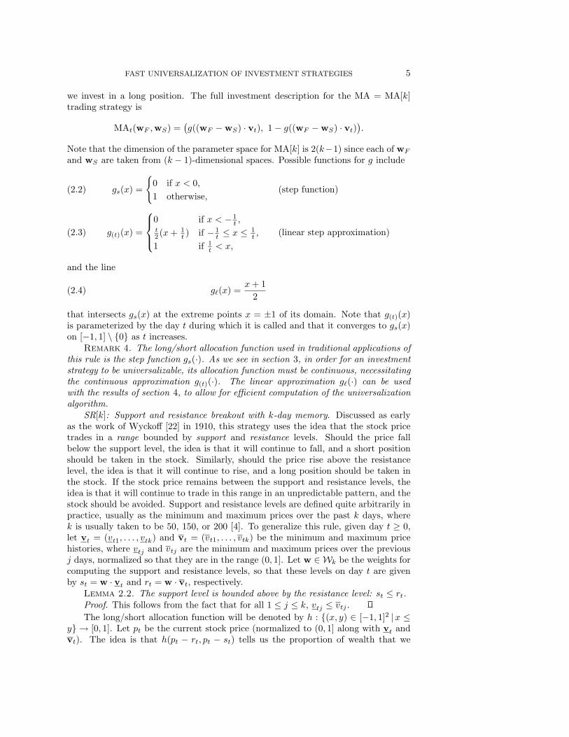
we invest in a long position. The full investment description for the MA = MA[k]trading strategy is

MAt(wF ,wS) =(g((wF − wS) · vt), 1 − g((wF − wS) · vt)

).

Note that the dimension of the parameter space for MA[k] is 2(k−1) since each of wF

and wS are taken from (k − 1)-dimensional spaces. Possible functions for g include

gs(x) =

0 if x < 0,

1 otherwise,(step function)(2.2)

g(t)(x) =

⎧⎪⎨⎪⎩

0 if x < − 1t ,

t2 (x + 1

t ) if − 1t ≤ x ≤ 1

t ,

1 if 1t < x,

(linear step approximation)(2.3)

and the line

g(x) =x + 1

2(2.4)

that intersects gs(x) at the extreme points x = ±1 of its domain. Note that g(t)(x)is parameterized by the day t during which it is called and that it converges to gs(x)on [−1, 1] \ 0 as t increases.

Remark 4. The long/short allocation function used in traditional applications ofthis rule is the step function gs(·). As we see in section 3, in order for an investmentstrategy to be universalizable, its allocation function must be continuous, necessitatingthe continuous approximation g(t)(·). The linear approximation g(·) can be usedwith the results of section 4, to allow for efficient computation of the universalizationalgorithm.

SR[k]: Support and resistance breakout with k-day memory. Discussed as earlyas the work of Wyckoff [22] in 1910, this strategy uses the idea that the stock pricetrades in a range bounded by support and resistance levels. Should the price fallbelow the support level, the idea is that it will continue to fall, and a short positionshould be taken in the stock. Similarly, should the price rise above the resistancelevel, the idea is that it will continue to rise, and a long position should be taken inthe stock. If the stock price remains between the support and resistance levels, theidea is that it will continue to trade in this range in an unpredictable pattern, and thestock should be avoided. Support and resistance levels are defined quite arbitrarily inpractice, usually as the minimum and maximum prices over the past k days, wherek is usually taken to be 50, 150, or 200 [4]. To generalize this rule, given day t ≥ 0,let vt = (vt1, . . . , vtk) and vt = (vt1, . . . , vtk) be the minimum and maximum pricehistories, where vtj and vtj are the minimum and maximum prices over the previousj days, normalized so that they are in the range (0, 1]. Let w ∈ Wk be the weights forcomputing the support and resistance levels, so that these levels on day t are givenby st = w · vt and rt = w · vt, respectively.

Lemma 2.2. The support level is bounded above by the resistance level: st ≤ rt.Proof. This follows from the fact that for all 1 ≤ j ≤ k, vtj ≤ vtj .

The long/short allocation function will be denoted by h : (x, y) ∈ [−1, 1]2 |x ≤y → [0, 1]. Let pt be the current stock price (normalized to (0, 1] along with vt andvt). The idea is that h(pt − rt, pt − st) tells us the proportion of wealth that we


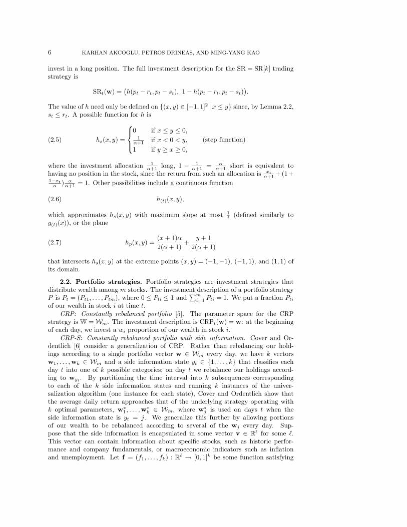
invest in a long position. The full investment description for the SR = SR[k] tradingstrategy is

SRt(w) =(h(pt − rt, pt − st), 1 − h(pt − rt, pt − st)

).

The value of h need only be defined on (x, y) ∈ [−1, 1]2 |x ≤ y since, by Lemma 2.2,st ≤ rt. A possible function for h is

hs(x, y) =

⎧⎪⎨⎪⎩

0 if x ≤ y ≤ 0,1

α+1 if x < 0 < y,

1 if y ≥ x ≥ 0,

(step function)(2.5)

where the investment allocation 1α+1 long, 1 − 1

α+1 = αα+1 short is equivalent to

having no position in the stock, since the return from such an allocation is xt

α+1 +(1+1−xt

α ) αα+1 = 1. Other possibilities include a continuous function

h(t)(x, y),(2.6)

which approximates hs(x, y) with maximum slope at most 1t (defined similarly to

g(t)(x)), or the plane

hp(x, y) =(x + 1)α

2(α + 1)+

y + 1

2(α + 1)(2.7)

that intersects hs(x, y) at the extreme points (x, y) = (−1,−1), (−1, 1), and (1, 1) ofits domain.

2.2. Portfolio strategies. Portfolio strategies are investment strategies thatdistribute wealth among m stocks. The investment description of a portfolio strategyP is Pt = (Pt1, . . . , Ptm), where 0 ≤ Pti ≤ 1 and

∑mi=1 Pti = 1. We put a fraction Pti

of our wealth in stock i at time t.CRP: Constantly rebalanced portfolio [5]. The parameter space for the CRP

strategy is W = Wm. The investment description is CRPt(w) = w: at the beginningof each day, we invest a wi proportion of our wealth in stock i.

CRP-S: Constantly rebalanced portfolio with side information. Cover and Or-dentlich [6] consider a generalization of CRP. Rather than rebalancing our hold-ings according to a single portfolio vector w ∈ Wm every day, we have k vectorsw1, . . . ,wk ∈ Wm and a side information state yt ∈ 1, . . . , k that classifies eachday t into one of k possible categories; on day t we rebalance our holdings accord-ing to wyt . By partitioning the time interval into k subsequences correspondingto each of the k side information states and running k instances of the univer-salization algorithm (one instance for each state), Cover and Ordentlich show thatthe average daily return approaches that of the underlying strategy operating withk optimal parameters, w∗

1, . . . ,w∗k ∈ Wm, where w∗

j is used on days t when theside information state is yt = j. We generalize this further by allowing portionsof our wealth to be rebalanced according to several of the wj every day. Sup-pose that the side information is encapsulated in some vector v ∈ R

for some .This vector can contain information about specific stocks, such as historic perfor-mance and company fundamentals, or macroeconomic indicators such as inflationand unemployment. Let f = (f1, . . . , fk) : R

→ [0, 1]k be some function satisfying


∑kj=1 fj(v) = 1 for all v ∈ R

. The parameter space is Wkm; the investment descrip-

tion is CRP-St(w1, . . . ,wk) =∑k

j=1 fj(vt)wj , where vt is the indicator vector forday t. Under such a scheme, we have the flexibility of splitting our wealth amongmultiple sets of portfolios w1, . . . ,wk on any given day, rather than being forced tochoose a single one. For example, assume that v is a k-dimensional vector, with eachvi corresponding to portfolio wi. Define f : R

k → [0, 1]k by fi(vt) = vti∑kι=1 vtι

, so that

our allocation is biased towards portfolios corresponding to higher indicators whilestill maintaining a position in the others.

IA[k]: k-way indicator aggregation. For each day t ≥ 0, suppose that each stock ihas a set of k indicators vti = (vti1, . . . , vtik), where each vtij ∈ (0, 1] and, for 1 ≤ j ≤k, vt1j , . . . , vtmj have been normalized such that there is at least one i such that vtij =1. Examples of possible indicators include historic stock performance and tradingvolumes, and company fundamentals. Our goal is to aggregate the indicators for eachstock to get a measure of the stock’s attractiveness and put a greater proportion of ourwealth in stocks that are more attractive. We will aggregate the indicators by takingtheir weighted average, where the weights will be determined by the parameters. Theparameter space is W = Wk, and the investment description is

IAt(w) =

(w · vt1∑mi=1 w · vti

, . . . ,w · vtm∑mi=1 w · vti

).

3. Universalization of investment strategies.

3.1. Universalization defined. In a typical stock market, wealth grows geo-metrically. On day t ≥ 0, let xt be the return vector for day t, the vector of factorsby which stock prices change on day t. The return vector corresponding to a tradingstrategy on a single stock is (xt, 1 + 1−xt

α ), where xt is the factor by which the price

of the stock changes and 1 + 1−xt

α is the factor by which our investment in a shortposition changes, as described in Lemma 2.1; the return vector corresponding to aportfolio strategy is (xt1, . . . , xtm), where xti is the factor by which the price of stocki changes, where 1 ≤ i ≤ m. Henceforth, we do not make a distinction betweenreturn vectors corresponding to trading and portfolio strategies; we assume that xt

is appropriately defined to correspond to the investment strategy in question. For aninvestment strategy S with parameter vector w, the return of S(w) during the tthday—the factor by which our wealth changes on the tth day when invested accordingto S(w)—is St(w) · xt =

∑mi=1 Sti(w) · xti. (Recall that St(w) is the investment

description of S(w) for day t, which is a vector specifying the proportion of wealth to

put in each stock.) Given time n > 0, let Rn(S(w)) =∏n−1

t=0 St(w) · xt be the cumu-lative return of S(w) up to time n; we may write Rn(w) in place of Rn(S(w)) if Sis obvious from context. We analyze the performance of S in terms of the normalizedlog-return Ln(w) = Ln(S(w)) = 1

n logRn(w) of the wealth achieved.

For investment strategy S, let w∗n = arg maxw∈R∗ Rn(S(w)) be the parameters

that maximize the return of S up to day n.4 An investment strategy U universalizes(or is universal for) S if5

Ln(U) = Ln(S(w∗n)) − o(1)

4As mentioned above, w∗n can be computed only with hindsight.

5Unlike previously discussed investment strategies, the behavior of U is fully defined without anadditional parameter vector w.


for all environment vectors En. That is, U is universal for S if the average dailylog-return of U approaches the optimal average daily log-return of S as the length nof the time horizon grows, regardless of stock price sequences.

3.2. General techniques for universalization. Given an investment strat-egy S, let W be the parameter space for S and let µ be the uniform measure overW. Our universalization algorithm for S, U(S), is a generalization of Cover’s originalresult [5]; we note that a similar algorithm appeared in [20] under the name “Aggre-gating Algorithm.” The investment description Ut(S) for the universalization of S onday t > 0 is a weighted average of St(w) over w ∈ W, with greater weight given toparameters w that have performed better in the past (i.e., Rt(w) is larger). Formally,the investment description is

Ut(S) =

∫WSt(w)Rt(w)dµ(w)∫WRt(w)dµ(w)

=

∫WSt(w)Rt(S(w))dµ(w)∫WRt(S(w))dµ(w)

,(3.1)

where we take R0(w) = 1 for all w ∈ W.6 Equivalently, the above integral mightbe interpreted as “splitting our money” equally among all the different strategies and“letting it sit.” In the following lemma, we will prove that this strategy has the sameexpected gain as picking one strategy at random.

Remark 5. The definition of universalization can be expanded to include mea-sures other than µ, but we consider only µ in our results.

Lemma 3.1 (see [3, 6]). The cumulative n-day return of U(S) is

Rn(U(S)) =

∫W

Rn(w)dµ(w) = E(Rn(w)

),

which is the µ-weighted average of the cumulative returns of the investment strategiesS(w) |w ∈ W.

Proof. The return of U(S) on day t is Ut(S) ·xt, where xt is the return vector forday t. The cumulative n-day return of U(S) is

Rn(U(S)) =

n−1∏t=0

Ut(S) · xt =

n−1∏t=0

∫WSt(w)Rt(w)dµ(w)∫WRt(w)dµ(w)

· xt

=

n−1∏t=0

∫W

(St(w) · xt)Rt(w)dµ(w)∫WRt(w)dµ(w)

=n−1∏t=0

∫WRt+1(w)dµ(w)∫

WRt(w)dµ(w)

.

The result follows from the fact that this product telescopes.Rather than directly universalizing a given investment strategy S, we instead

focus on a modified version of S that puts a nonzero fraction of wealth into each ofthe m stocks. Define the investment strategy S by

St(w) =

(1 − ε

2(t + 1)2

)St(w) +

ε

2m(t + 1)2

for t ≥ 0 and some fixed 0 < ε < 1. Rather than universalizing S, we insteaduniversalize S. Lemma 3.2 tells us that we do not lose much by doing this.

Lemma 3.2. For all n ≥ 0, (1) Rn(U(S)) ≥ (1−ε)Rn(U(S)) and (2) Ln(U(S)) =

Ln(U(S))− o(n)n . (3) If U(S) is a universalization of S, then U(S) is a universalization

of S as well.

6Cover’s algorithm is a special case of this, replacing St(w) with w.


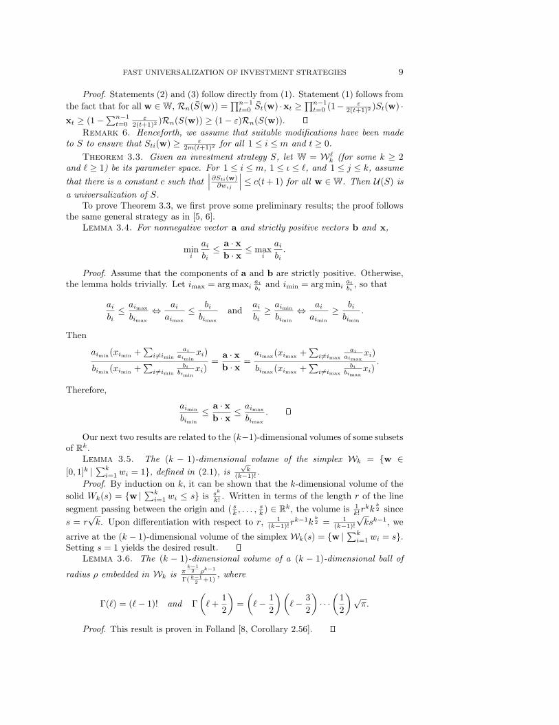
Proof. Statements (2) and (3) follow directly from (1). Statement (1) follows from

the fact that for all w ∈ W, Rn(S(w)) =∏n−1

t=0 St(w) ·xt ≥∏n−1

t=0 (1− ε2(t+1)2 )St(w) ·

xt ≥ (1 −∑n−1

t=0ε

2(t+1)2 )Rn(S(w)) ≥ (1 − ε)Rn(S(w)).

Remark 6. Henceforth, we assume that suitable modifications have been madeto S to ensure that Sti(w) ≥ ε

2m(t+1)2 for all 1 ≤ i ≤ m and t ≥ 0.

Theorem 3.3. Given an investment strategy S, let W = Wk (for some k ≥ 2

and ≥ 1) be its parameter space. For 1 ≤ i ≤ m, 1 ≤ ι ≤ , and 1 ≤ j ≤ k, assume

that there is a constant c such that∣∣∣∂Sti(w)

∂wιj

∣∣∣ ≤ c(t+ 1) for all w ∈ W. Then U(S) is

a universalization of S.To prove Theorem 3.3, we first prove some preliminary results; the proof follows

the same general strategy as in [5, 6].Lemma 3.4. For nonnegative vector a and strictly positive vectors b and x,

mini

aibi

≤ a · xb · x ≤ max

i

aibi.

Proof. Assume that the components of a and b are strictly positive. Otherwise,the lemma holds trivially. Let imax = arg maxi

ai

biand imin = arg mini

ai

bi, so that

aibi

≤ aimax

bimax

⇔ aiaimax

≤ bibimax

andaibi

≥ aimin

bimin

⇔ aiaimin

≥ bibimin

.

Then

aimin(ximin

+∑

i =imin

ai

aiminxi)

bimin(ximin

+∑

i =imin

bibimin

xi)=

a · xb · x =

aimax(ximax+∑

i =imax

ai

aimaxxi)

bimax(ximax

+∑

i =imax

bibimax

xi).

Therefore,

aimin

bimin

≤ a · xb · x ≤ aimax

bimax

.

Our next two results are related to the (k−1)-dimensional volumes of some subsetsof R

k.Lemma 3.5. The (k − 1)-dimensional volume of the simplex Wk = w ∈

[0, 1]k |∑k

i=1 wi = 1, defined in (2.1), is√k

(k−1)! .

Proof. By induction on k, it can be shown that the k-dimensional volume of the

solid Wk(s) = w |∑k

i=1 wi ≤ s is sk

k! . Written in terms of the length r of the line

segment passing between the origin and ( sk , . . . ,

sk ) ∈ R

k, the volume is 1k!r

kkk2 since

s = r√k. Upon differentiation with respect to r, 1

(k−1)!rk−1k

k2 = 1

(k−1)!

√ksk−1, we

arrive at the (k − 1)-dimensional volume of the simplex Wk(s) = w |∑k

i=1 wi = s.Setting s = 1 yields the desired result.

Lemma 3.6. The (k − 1)-dimensional volume of a (k − 1)-dimensional ball of

radius ρ embedded in Wk is πk−12 ρk−1

Γ( k−12 +1)

, where

Γ() = (− 1)! and Γ

( +

1

2

)=

(− 1

2

)(− 3

2

)· · ·

(1

2

)√π.

Proof. This result is proven in Folland [8, Corollary 2.56].


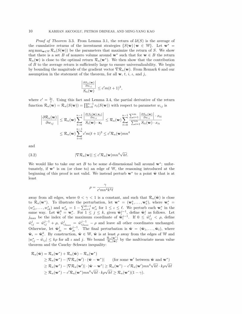
Proof of Theorem 3.3. From Lemma 3.1, the return of U(S) is the average ofthe cumulative returns of the investment strategies S(w) |w ∈ W. Let w∗ =arg maxw∈W Rn(S(w)) be the parameters that maximize the return of S. We showthat there is a set B of nonzero volume around w∗ such that for w ∈ B the returnRn(w) is close to the optimal return Rn(w∗). We then show that the contributionof B to the average return is sufficiently large to ensure universalizability. We beginby bounding the magnitude of the gradient vector ∇Rn(w). From Remark 6 and ourassumption in the statement of the theorem, for all w, t, i, ι, and j,∣∣∣∂Sti(w)

∂wιj

∣∣∣Sti(w)

≤ c′m(t + 1)3,

where c′ = 2cε . Using this fact and Lemma 3.4, the partial derivative of the return

function Rn(w) = Rn(S(w)) =∏n−1

t=0 rt(S(w)) with respect to parameter wιj is

∣∣∣∣∂Rn(w)

∂wιj

∣∣∣∣ ≤ Rn(w)

n−1∑t=0

∣∣∣∂(St(w)·xt)∂wιj

∣∣∣St(w) · xt

≤ Rn(w)

n−1∑t=0

∑mi=1

∣∣∣∂Sti(w)∂wιj

∣∣∣ · xti∑mi=1 Sti(w) · xti

≤ Rn(w)

n−1∑t=0

c′m(t + 1)3 ≤ c′Rn(w)mn4

and

|∇Rn(w)| ≤ c′Rn(w)mn4√k.(3.2)

We would like to take our set B to be some d-dimensional ball around w∗; unfor-tunately, if w∗ is on (or close to) an edge of W, the reasoning introduced at thebeginning of this proof is not valid. We instead perturb w∗ to a point w that is atleast

ρ =γ

c′mn4k2

away from all edges, where 0 < γ < 1 is a constant, and such that Rn(w) is closeto Rn(w∗). To illustrate the perturbation, let w∗ = (w∗

1, . . . ,w∗ ), where w∗

ι =

(w∗ι1, . . . , w

∗ιk) and w∗

ιk = 1 −∑k−1

i=1 w∗ιi for 1 ≤ ι ≤ . We perturb each w∗

ι in thesame way. Let w0

ι = w∗ι . For 1 ≤ j ≤ k, given wj−1

ι , define wjι as follows. Let

jmax be the index of the maximum coordinate of wj−1ι . If 0 ≤ wj

ιj < ρ, define

wjιj = wj−1

ιj + ρ, wjιjmax

= wj−1ιjmax

− ρ and leave all other coordinates unchanged.

Otherwise, let wjj0

= wj−1j0

. The final perturbation is w = (w1, . . . , w), where

wι = wkι . By construction, w ∈ W, w is at least ρ away from the edges of W and

|w∗ιj − wιj | ≤ kρ for all ι and j. We bound Rn(w∗)

Rn(w) by the multivariate mean value

theorem and the Cauchy–Schwarz inequality:

Rn(w) = Rn(w∗) + Rn(w) −Rn(w∗)

≥ Rn(w∗) − |∇Rn(w′) · (w − w∗)| (for some w′ between w and w∗)

≥ Rn(w∗) − |∇Rn(w′)| · |w − w∗| ≥ Rn(w∗) − c′Rn(w′)mn4√k · kρ

√k

≥ Rn(w∗) − c′Rn(w∗)mn4√k · kρ

√k ≥ Rn(w∗)(1 − γ).


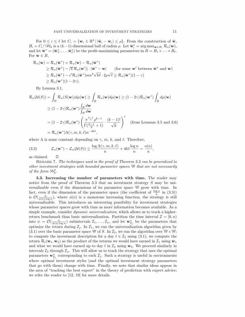
For 0 ≤ ι ≤ let Cι = wι ∈ Rk | |wι − wι| ≤ ρ. From the construction of w,

Bι = Cι∩Wk is a (k−1)-dimensional ball of radius ρ. Let w∗ι = arg maxw∈Bι Rn(w),

and let w∗ = (w∗1, . . . , w

∗ ) be the profit-maximizing parameters in B = B1×· · ·×B.

For w ∈ B,

Rn(w) = Rn(w∗) + Rn(w) −Rn(w∗)

≥ Rn(w∗) − |∇Rn(w′)| · |w∗ − w| (for some w′ between w∗ and w)

≥ Rn(w∗) − c′Rn(w∗)mn4√k · 2ρ

√ ≥ Rn(w∗)(1 − γ)

≥ Rn(w∗)(1 − 2γ).

By Lemma 3.1,

Rn(U(S)) =

∫W

Rn(S(w))dµ(w) ≥∫B

Rn(w)dµ(w) ≥ (1 − 2γ)Rn(w∗)

∫B

dµ(w)

≥ (1 − 2γ)Rn(w∗)

∫Bdw∫

Wdw

= (1 − 2γ)Rn(w∗)

(π

k−12 ρk−1

Γ(k−12 + 1)

· (k − 1)!√k

)

(from Lemmas 3.5 and 3.6)

= Rn(w∗)Λ(γ,m, k, )n−4k,

where Λ is some constant depending on γ, m, k, and . Therefore,

Ln(w∗) − Ln(U(S)) ≤ log Λ(γ,m, k, )

n+ 4k

log n

n=

o(n)

n,(3.3)

as claimed.Remark 7. The techniques used in the proof of Theorem 3.3 can be generalized to

other investment strategies with bounded parameter spaces W that are not necessarilyof the form W

k.

3.3. Increasing the number of parameters with time. The reader maynotice from the proof of Theorem 3.3 that an investment strategy S may be uni-versalizable even if the dimensions of its parameter space W grow with time. Infact, even if the dimension of the parameter space (the coefficient of log n

n in (3.3))is O( n

φ(n) log n ), where φ(n) is a monotone increasing function, the strategy is still

universalizable. This introduces an interesting possibility for investment strategieswhose parameter spaces grow with time as more information becomes available. As asimple example, consider dynamic universalization, which allows us to track a higher-return benchmark than basic universalization. Partition the time interval I = [0, n)into ψ = O( n

φ(n) log n ) subintervals I1, . . . , Iψ, and let w∗Ij

be the parameters that

optimize the return during Ij . In I1, we run the universalization algorithm given by(3.1) over the basic parameter space W of S. In I2, we run the algorithm over W×W;to compute the investment description for a day t ∈ I2 using (3.1), we compute thereturn Rt(w1,w2) as the product of the returns we would have earned in I1 using w1

and what we would have earned up to day t in I2 using w2. We proceed similarly inintervals I3 through Iψ. This will allow us to track the strategy that uses the optimalparameters w∗

Ijcorresponding to each Ij . Such a strategy is useful in environments

where optimal investment styles (and the optimal investment strategy parametersthat go with them) change with time. Finally, we note that similar ideas appear inthe area of “tracking the best expert” in the theory of prediction with expert advice;we refer the reader to [12, 19] for more details.


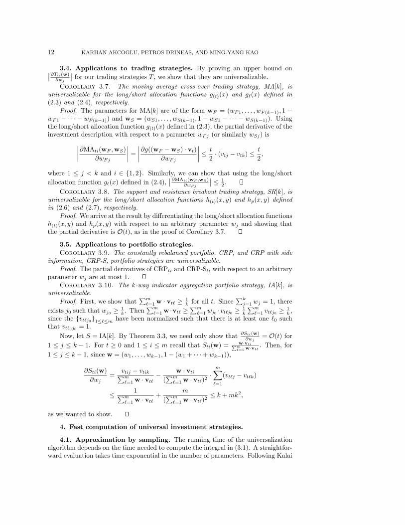
3.4. Applications to trading strategies. By proving an upper bound on∣∣∂Tti(w)∂wj

∣∣ for our trading strategies T , we show that they are universalizable.

Corollary 3.7. The moving average cross-over trading strategy, MA[k], isuniversalizable for the long/short allocation functions g(t)(x) and g(x) defined in(2.3) and (2.4), respectively.

Proof. The parameters for MA[k] are of the form wF = (wF1, . . . , wF (k−1), 1 −wF1 − · · · − wF (k−1)) and wS = (wS1, . . . , wS(k−1), 1 − wS1 − · · · − wS(k−1)). Usingthe long/short allocation function g(t)(x) defined in (2.3), the partial derivative of theinvestment description with respect to a parameter wFj (or similarly wSj) is∣∣∣∣∂MAti(wF ,wS)

∂wFj

∣∣∣∣ =

∣∣∣∣∂g((wF − wS) · vt)

∂wFj

∣∣∣∣ ≤ t

2· (vtj − vtk) ≤

t

2,

where 1 ≤ j < k and i ∈ 1, 2. Similarly, we can show that using the long/short

allocation function g(x) defined in (2.4),∣∣∂MAti(wF ,wS)

∂wFj

∣∣ ≤ 12 .

Corollary 3.8. The support and resistance breakout trading strategy, SR[k], isuniversalizable for the long/short allocation functions h(t)(x, y) and hp(x, y) definedin (2.6) and (2.7), respectively.

Proof. We arrive at the result by differentiating the long/short allocation functionsh(t)(x, y) and hp(x, y) with respect to an arbitrary parameter wj and showing thatthe partial derivative is O(t), as in the proof of Corollary 3.7.

3.5. Applications to portfolio strategies.

Corollary 3.9. The constantly rebalanced portfolio, CRP, and CRP with sideinformation, CRP-S, portfolio strategies are universalizable.

Proof. The partial derivatives of CRPti and CRP-Sti with respect to an arbitraryparameter wj are at most 1.

Corollary 3.10. The k-way indicator aggregation portfolio strategy, IA[k], isuniversalizable.

Proof. First, we show that∑m

=1 w · vt ≥ 1k for all t. Since

∑kj=1 wj = 1, there

exists j0 such that wj0 ≥ 1k . Then

∑m=1 w ·vt ≥

∑m=1 wj0 ·vtj0 ≥ 1

k

∑m=1 vtj0 ≥ 1

k ,since the vtj01≤≤m have been normalized such that there is at least one 0 suchthat vt0j0 = 1.

Now, let S = IA[k]. By Theorem 3.3, we need only show that ∂Sti(w)∂wj

= O(t) for

1 ≤ j ≤ k − 1. For t ≥ 0 and 1 ≤ i ≤ m recall that Sti(w) = w·vti∑m=1 w·vt

. Then, for

1 ≤ j ≤ k − 1, since w = (w1, . . . , wk−1, 1 − (w1 + · · · + wk−1)),

∂Sti(w)

∂wj=

vtij − vtik∑m=1 w · vt

− w · vti

(∑m

=1 w · vt)2·

m∑=1

(vtj − vtk)

≤ 1∑m=1 w · vt

+m

(∑m

=1 w · vt)2≤ k + mk2,

as we wanted to show.

4. Fast computation of universal investment strategies.

4.1. Approximation by sampling. The running time of the universalizationalgorithm depends on the time needed to compute the integral in (3.1). A straightfor-ward evaluation takes time exponential in the number of parameters. Following Kalai


and Vempala [14], we propose to approximate this integral by sampling the param-eters according to a biased distribution, giving greater weight to better performingparameters. Define the measure ζt on W by

dζt(w) =Rt(S(w))∫

WRt(S(w))dµ(w)

dµ(w).

Lemma 4.1 (see [14]). The investment description Ut(S) for universalization isthe average of St(w) with respect to the ζt measure.

Proof. The average of St(w) with respect to ζt is

Ew∈(W,ζt)(St(w)) =

∫W

St(w)dζt(w)

=

∫W

St(w)Rt(S(w))∫

WRt(S(w))dµ(w)

dµ(w) = Ut(S),

where the final equality follows from (3.1).We now briefly outline our approach, which follows the lines of [2, 14]. The main

technical complication is that sampling efficiently with respect to ζt is not, in general,an easy problem. As a result, we will need some (rather generic) assumption on theinvestment strategies from which we can sample efficiently.

• Investment strategies with log-concavity properties. In section 4.3, we usestraightforward manipulations to prove that any investment strategy S whichis linear in the vector of parameters w (such strategies include MA[k], SR[k],CRP, and CRP-S) has a cumulative return function Rt(S(w)) that is log-concave. Our efficient sampling techniques are applicable only on such strate-gies.

• Approximating ζt by ζt. In section 4.2, we show that for strategies whosecumulative return function is log-concave, it is possible to efficiently samplefrom a distribution ζt that is “close” to ζt. This “distribution approximation”incurs some small, bounded error (see Lemma 4.2).

• Approximating the integral for ζt via sampling. With such sampling abilities,it is easy to approximate the average of St(w) with respect to ζt: simply pickNt (as defined in Lemma 4.3) sample parameter vectors w with respect to ζtand compute their average. The error incurred by this approximation of theaverage can be bounded in a straightforward manner using Chernoff bounds.

• Sampling with respect to ζt. The critical issue (addressed in section 4.2) ishow to pick vectors w ∈ W with respect to ζt. In order to tackle this problem,we “discretize” it by placing a grid on W, and then we perform a Metropolisrandom walk. The convergence properties of this random walk are discussedin Theorems 4.12 and 4.13.

In section 4.2, we show that for certain strategies we can efficiently sample froma distribution ζt that is “close” to ζt; i.e., given γt > 0, we generate samples from ζtsuch that ∫

W

∣∣ζt(w) − ζt(w)∣∣ dµ(w) ≤ γt.(4.1)

Assume for now that we can sample from ζt, with γt = ε2

4m(t+1)4 , where ε is the

constant appearing in Remark 6. Let Ut(S) =∫

WSt(w)dζt(w) be the corresponding


approximation to U(S). Lemma 4.2 tells us that we do not lose much by samplingfrom ζt.

Lemma 4.2. For all n ≥ 0, (1) Rn(U(S)) ≥ (1− ε)Rn(U(S)) and (2) if U(S) isa universalization of S, then U(S) is a universalization of S as well.

Proof. Statement (2) follows directly from (1). To see (1), we need only showthat the fraction of wealth that we put into each stock i on day t under U(S) is withina 1 − ε

2(t+1)2 factor of the corresponding amount under U(S); i.e., Uti(S) ≥ (1 −ε

2(t+1)2 )Uti(S) for 0 ≤ t < n and 1 ≤ i ≤ m. For w ∈ W, let γt(w) = |ζt(w) − ζt(w)|,so that

∫Wγt(w)dw = γt ≤ ε2

4m(t+1)4 . We have

Uti(S) =

∫W

Sti(w)ζt(w)dµ(w) ≥∫

W

Sti(w)(ζt(w) − γt(w))dµ(w)

= Uti(S) −∫

W

Sti(w)γt(w)dµ(w) ≥ Uti(S) − γt (since Sti(w) ≤ 1)

≥(

1 − ε

2(t + 1)2

)Uti(S)(

since Uti(S) ≥ minw

S(w) ≥ ε

2m(t + 1)2and γt ≤ ε2

4m(t+1)4

),

as we wanted to show.

By sampling from ζt, we use a generalization of the Chernoff bound to get an ap-proximation U(S) to U(S) such that with high probability Uti(S) ≥ (1− ε

2(t+1)2 )Uti(S)

for 0 ≤ t < n and 1 ≤ i ≤ m. Using an argument similar to that in the proof ofLemma 4.2, we see that if U(S) is a universalization of S, then such a U(S) is a univer-salization of S as well. Choose w1, . . . ,wNt ∈ W at random according to distribution

ζt, and let Uti(S) = 1Nt

∑Nt

i=1 Sti(wi). Lemma 4.3 discusses the number of samples Nt

required to get a sufficiently good approximation to Ut(S).

Lemma 4.3. Given 0 < δ < 1, use Nt ≥ 8m2(t+1)8

ε4 log 2m(t+1)2

δ samples to

compute Ut(S), where ε is the constant appearing in Remark 6. With probability1 − δ, Uti(S) ≥ (1 − ε

2(t+1)2 )Uti(S) for all 1 ≤ i ≤ m and t ≥ 0.

Proof. Hoeffding [13] proves a general version of the Chernoff bound. For random

variables 0 ≤ Xi ≤ 1 with E(Xi) = µ and X = 1N

∑Ni=1 Xi, the bound states that

Pr(X ≤ (1 − α)µ) ≤ e−2Nα2µ2

. In our case, we would like Uti ≥ (1 − ε2(t+1)2 )Uti.

As this must hold for 1 ≤ i ≤ m and t ≥ 0 with total probability 1 − δ, we requirePr(Uti ≤ (1 − ε

2(t+1)2 )Uti) ≤ δ2m(t+1)2 for each i and t. From our assumption stated

in Remark 6, µ = Uti ≥ ε2m(t+1)2 , and the desired probability bound is achieved with

Nt ≥ 8m2(t+1)8

ε4 log 2m(t+1)2

δ samples.

4.2. Efficient sampling. We now discuss how to sample from W = Wk =

Wk × · · · ×Wk according to distribution ζt(·) ∝ Rt(·) = Rt(S(·)). W is a convex setof diameter d =

√2. We focus on a discretization of the sampling problem. Choose

an orthogonal coordinate system on each Wk, and partition it into hypercubes of sidelength δt, where δt is a constant chosen below. Let Ω be the set of centers of cubesthat intersect W, and choose the partition such that the coordinates of w ∈ Ω aremultiples of δt. For w ∈ Ω, let C(w) be the cube with center w. We show how to


choose w ∈ Ω with probability “close to”

πt(w) =Rt(w)∑

w∈Ω Rt(w).

In particular, we sample from a distribution πt that satisfies

∑w∈Ω

|πt(w) − πt(w)| ≤ γt =ε2

4m(t + 1)4.(4.2)

Note that this is a discretization of (4.1). We will also have that for each w ∈ Ω,

πt(w)

πt(w)≤ 2.(4.3)

We would like to choose δt sufficiently small that Rt is “nearly constant” over C(w);i.e., there is a small constant ν > 0 such that

(1 + ν)−1Rt(w) ≤ Rt(w′) ≤ (1 + ν)Rt(w)(4.4)

for all w′ ∈ C(w). Such a δt can be chosen for investment strategies S that havebounded derivative, as we see in Lemma 4.4.

Lemma 4.4. Suppose that investment strategy S satisfies the condition for uni-

versalizability given in Theorem 3.3; i.e.,∣∣∂Sti(w)

∂wj

∣∣ ≤ c(t + 1). Given ν > 0, let

δt = δt(ν) = ν3c′mt4k , where c′ is defined in the proof of Theorem 3.3. For w,w′ ∈ W

such that |wij − w′ij | ≤ δt(ν) for all 1 ≤ i ≤ and 1 ≤ j ≤ k, (1 + ν)−1Rt(w) ≤

Rt(w′) ≤ (1 + ν)Rt(w).

Proof. Note that |w−w′| ≤ δt√k. Let w∗ be the parameters that maximize the

return on the line between w and w′. By the multivariate mean value theorem andthe bound for |∇Rt| given in (3.2),

Rt(w∗) = Rt(w) + Rt(w

∗) −Rt(w)

≤ Rt(w) + |∇Rt(wm)| · |w − w∗| (for some wm between w∗ and w)

≤ Rt(w) + c′Rt(wm)mn4√k · δt

√k ≤ Rt(w) + Rt(w

∗)ν

3

⇒ Rt(w) ≥ Rt(w∗)

(1 − ν

3

)≥ Rt(w

′)(1 − ν

3

)so that Rt(w

′) ≤ (1 + ν)Rt(w). By similar reasoning,

Rt(w′) = Rt(w

∗) + Rt(w′) −Rt(w

∗)

≥ Rt(w∗) − |∇Rt(wm)| · |w′ − w∗| (for some wm between w∗ and w′)

≥ Rt(w∗)

(1 − ν

3

)≥ Rt(w)

(1 − ν

3

)≥ Rt(w)(1 + ν)−1,

completing the proof.We use a Metropolis algorithm [15] to sample from πt. We generate a random

walk on Ω according to a Markov chain whose stationary distribution is πt. Begin byselecting a point w0 ∈ Ω according to either πt−1 or πt−2;

7 Remark 8 explains howto do this.

7Ideally, we would like to begin with a point selected according to πt−1, but, as discussed inRemark 8, this is not always possible.


Remark 8. We can select a point according to πt−1 by “saving” our sam-ples that were generated at time t − 1. By Lemma 4.3, we would have generated

Nt−1 ≥ 8m2t8

ε4 log 2mt2

δ samples at time t − 1, which is not enough to generate the

Nt ≥ 8m2(t+1)8

ε4 log 2m(t+1)2

δ samples necessary at time t. Instead, we can “save”samples that were generated at times t − 1 and t − 2. For sufficiently large t, Nt ≤Nt−1 + Nt−2 and our initial point w0 would be picked according to either πt−1 orπt−2. As we see in the proof of Lemma 4.10, this distinction is not important.

If wτ is the position of our random walk at time τ ≥ 0, we pick its position attime τ + 1 as follows. Note that wτ has 2(k − 1) neighbors, two along each axis inthe Cartesian product of (k − 1)-dimensional spaces. Let w be a neighbor of wτ ,selected uniformly at random. If w ∈ Ω, set

wτ+1 =

w with probability p = min(1, Rt(w)

Rt(wτ ) ),

wτ with probability 1 − p.

If w ∈ Ω, let wτ+1 = wτ . It is well known that the stationary distribution of thisrandom walk is πt. We must determine how many steps of the walk are necessarybefore the distribution has gotten sufficiently close to stationary. Let pτ be the dis-tribution attained after τ steps of the random walk. That is, pτ (w) is the probabilityof being at w after τ steps.

Remark 9. A distinction should be made between t and τ . We use t to referto the time step in our universalization algorithm. We use τ to refer to “sub-” timesteps used in the Markov chain to sample from πt. When t is clear from context, wemay drop it from the subscripts in our notation.

Applegate and Kannan [2] show that if the desired distribution πt is proportionalto a log-concave function F (i.e., logF is concave), then the Markov chain is rapidlymixing and reaches its steady state in polynomial time. Frieze and Kannan [9] give animproved upper bound on the mixing time using logarithmic Sobolev inequalities [7].

Theorem 4.5 (Theorem 1 of [9]). Assume the diameter d of W satisfies d ≥δt√k and that the target distribution π is proportional to a log-concave function.

There is an absolute constant κ > 0 such that

2

(∑w∈Ω

|π(w) − pτ (w)|)2

≤ e−κτδ2tkd2 log

1

π∗+

Mπekd2

κδ2t

,(4.5)

where π∗ = minw∈Ω π(w), M = maxw∈Ωp0(w)π(w) log p0(w)

π(w) , p0(·) is the initial distribu-

tion on Ω, πe =∑

w∈Ωeπ(w), and Ωe = w ∈ Ω |Vol(C(w) ∩ W) < Vol(C(w)).

(The “e” in the subscripts of πe and Ωe stands for “edge.”)In the random walk described above, if wτ is on an edge of Ω, so that it has many

neighbors outside Ω, the walk may get “stuck” at wτ for a long time, as seen in the“πe” term of Theorem 4.5. We must ensure that the random walk has a low probabilityof reaching such edge points. We do this by applying a “damping function” to Rt,which becomes exponentially small near the edges of W. For 1 ≤ i ≤ , 1 ≤ j ≤ k,and w = (w1, . . . ,w) = ((w11, . . . , w1k), . . . , (w1, . . . , wk)) ∈ W let

fij(w) = eΓ min(−σ+wij ,0),(4.6)

where σ > 0 and Γ > 2 are constants that we choose below, and let

Ft(w) = Rt(w)

∏i=1

k∏j=1

fij(w).


Lemma 4.6. Ft is log-concave if and only if Rt is log-concave.8

Proof. This follows from the fact that log-concave functions are closed under mul-tiplication and the fact that log fij(w) = Γ min(−σ + wij , 0), which is concave.

Choose σ = 1k δt(

γt

2 ), where δt(·) is defined in Lemma 4.4 and γt is defined in(4.2). Let ζF ∝ Ft be the probability measure proportional to Ft. We need to showthat, for our purposes, sampling from ζF is not much different than sampling from ζt.By Lemma 4.2, we can do this by showing that

∫W|ζt(w)− ζF (w)|dw ≤ γt, which we

do in Lemma 4.7.

Remark 10. Before continuing, we show how W can be scaled, which will beuseful in future proofs. Take p = ( 1

k , . . . ,1k ) ∈ Wk; given χ ∈ (−1, 1), let

w(χ) = (1 + χ)(w − p) + p,

and let

W(χ)k = w(χ) |w ∈ Wk

be a scaled version of Wk about p, where the scaling factor is 1 + χ. To extend this

scaling to W = Wk, given w = (w1, . . . ,w) ∈ W, let w(χ) = (w

(χ)1 , . . . ,w

(χ) ) and

W(χ) = w(χ) |w ∈ W.

A fact we use is that for 1 ≤ i ≤ , 1 ≤ j ≤ k, and w = (w1, . . . ,w) ∈ W,

|w(χ)ij − wij | =

∣∣∣∣(1 + χ)

(wij −

1

k

)+

1

k− wij

∣∣∣∣ ≤ |χ|.

Lemma 4.7.

∫W|ζt(w) − ζF (w)|dw ≤ γt.

Proof. Let W′ = W

(−kσ) be the “scaled-in” version of W, as defined in Remark 10.By Lemma 4.4, since |wij − w′

ij | ≤ kσ = δt(γt

2 ) for all i and j, Rt(w′) ≥ 1

1+γt2Rt(w)

and ∫W′

Rt(w)dw ≥ 1

1 + γt

2

∫W

Rt(w)dw.(4.7)

Let Weq = w ∈ W |Ft(w) = Rt(w) be the subset of W where Ft(·) and Rt(·)are equal; W

′ ⊂ Weq since, by construction of w′, w′ij ≥ σ for all i and j. Let

W+ = w ∈ W | ζF (w) ≥ ζt(w) be the subset of W where ζF (·) is at least ζt(·) andlet W− = W − W+. We bound∫

W

|ζF (w) − ζt(w)|dw =

∫W+

(ζF (w) − ζt(w))dw +

∫W−

(ζt(w) − ζF (w))dw

by bounding∫

W−(ζt − ζF ), which also gives a bound for

∫W+

(ζF − ζt), since

∫W+

(ζF − ζt) =

(1 −

∫W−

ζF

)−(

1 −∫

W−

ζt

)=

∫W−

(ζt − ζF ).

8We characterize investment strategies for which Rt is log-concave in Theorem 4.14.


Since Ft ≤ Rt,∫

WFt ≤

∫WRt and ζF (w) = Ft(w)∫

WFt

≥ Rt(w)∫WRt

= ζt(w) for w ∈ Weq;

thus W′ ⊂ Weq ⊂ W+ and W− ⊂ W − W

′. We have

∫W−

(ζt(w) − ζF (w))dw ≤∫

W−W′ζt(w)dw =

∫W−W′ Rt(w)dw∫

WRt(w)dw

= 1 −∫

W′ Rt(w)dw∫WRt(w)dw

≤ 1 − 1

1 + γt

2

≤ γt2,

where the second-to-last inequality follows from (4.7). This completes the proof.

Henceforth, we are concerned with sampling from W with probability proportionalto Ft(·). We use the Metropolis algorithm described above, replacing Rt(·) with Ft(·);we must refine our grid spacing δt so that (4.4) is satisfied by Ft; let δ′t be the newgrid spacing.

Lemma 4.8. Suppose that the conditions of Lemma 4.4 are satisfied. Givenν > 0, let δ′t(ν) = δ′t = ν

3Γc′mt4k = δt(νΓ ), where Γ appears in (4.6). For w,w′ ∈ W

such that |wij − w′ij | ≤ δ′t(ν) for all 1 ≤ i ≤ and 1 ≤ j ≤ k, (1 + ν)−1Ft(w) ≤

Ft(w′) ≤ (1 + ν)Ft(w).

Proof. By Lemma 4.4, Rt(w) and Rt(w′) differ by at most a factor of 1 + ν

Γ .

For each i and j, fij(w) and fij(w′) differ by at most a factor of eΓδ′t(ν), and hence∏

i=1

∏kj=1 fij(w) and

∏i=1

∏kj=1 fij(w

′) differ by at most a factor of ekΓδ′t(ν) =

eν

3c′mt4 . Hence, for Γ ≥ 2 and sufficiently large t, Ft(w) and Ft(w′) differ by at most

a factor of 1 + ν.

We are now ready to use Theorem 4.5 to select τ so that the resulting distributionpτ satisfies (4.2) (Theorem 4.12) and (4.3) (Theorem 4.13), with pτ in place of πt andFt in place of Rt. We begin with some preliminary lemmas.

Lemma 4.9. There is a constant β > 0 such that log 1π∗

≤ kΓσ + k log βδ′t

+t log 2mt2

ε , where ε is defined in Remark 6.

Proof. Take β such that the number of points in Ω is at most ( βδ′t

)(k−1)·. For

w1,w2 ∈ Ω, the ratio of single-day returns on day t′ using w1 and w2 is

St′(w1) · xt′

St′(w2) · xt′≥ ε

2m(t′ + 1)2,

by Remark 6 and Lemma 3.4. The ratio of the cumulative returns up to day t is

Rt(w1)

Rt(w2)≥

( ε

2mt2

)t

,

and thus Rt(w)∑w∈Ω Rt(w) ≥ (

δ′tβ )(k−1)

(ε

2mt2

)t. Factoring in the maximum dampening

effect of the fij , π∗ ≥ e−kΓσ(δ′tβ )(k−1)

(ε

2mt2

)tand log 1

π∗≤ kΓσ + k log β

δ′t+

t log 2mt2

ε .

Lemma 4.10. M ≤ 4( 2m(t+1)2

ε

)2log 2m(t+1)2

ε .

Proof. As stated in Remark 8, the initial distribution is either p0 = πt−1 or πt−2.

It turns out that the worst case happens when p0 = πt−2. For all w ∈ Ω, πt−2(w)πt−2(w) ≤ 2

by (4.3) and the following:


πt−2(w)

πt(w)=

Ft−2(w)∑w∈Ω Ft−2(w)

·∑

w∈Ω Ft(w)

Ft(w)

≤ Ft−2(w)

Ft(w)· Ft(w

′)

Ft−2(w′)

(by Lemma 3.4, where w′ = arg max

w∈Ω

Ft(w)

Ft−2(w)

)

=Rt−2(w)

Rt(w)· Rt(w

′)

Rt−2(w′)(since the fij(·)i,j remain constant with time)

=(St(w

′) · xt)(St−1(w′) · xt−1)

(St(w) · xt)(St−1(w) · xt−1)≤

(2m(t + 1)2

ε

)2

,

where the final inequality follows from the discussion in the proof of Lemma 4.9. This

proves the result since πt−2(w)πt(w) = πt−2(w)

πt−2(w)

πt−2(w)

πt(w) .

Lemma 4.11. πe ≤ (1 + ν)4(1 + γt

2 )e−Γσ, where ν appears in the definition of δ′tin Lemma 4.8, γt appears in (4.2), and Γ and σ appear in (4.6).

Proof. Extend our δ′t-hypercube partition of W to the hyperplane containing W,and let Ψ be the set of centers of the hypercubes in this extended partition. ForK ⊂ R

k, let ΨK be the set of grid points w ∈ Ψ such that C(w) ∩K = ∅, so thatΩ = ΨW. By Lemma 4.8, for K ⊂ W,

1

1 + ν

∑w∈ΨK

Ft(w)Vol(C(w) ∩K) ≤∫K

Ft(w)dw ≤ (1 + ν)∑

w∈ΨK

Ft(w)Vol(C(w) ∩K).

(4.8)

Using the notation of Lemma 4.7, let W′ = W

(−kσ) be a “scaled-in” version of W; weshowed in Lemma 4.7 that for w ∈ W

′, Ft(w) = Rt(w), and that∫W′

Ft(w)dw =

∫W′

Rt(w)dw ≥ 1

1 + γt

2

∫W

Rt(w)dw.(4.9)

Let W′′ = W

(δ′t(ν)) be a “scaled-out” version of W, and extend the domains of Ft(·) andRt(·) to W

′′ by defining Ft(w′′) = Ft(w

′′) and Rt(w′′) = Rt(w

′′) for w′′ ∈ W′′ − W,

where w′′ is the point where the line between w′′ and p = (p, . . . ,p) ∈ W intersectsthe boundary of W. By Lemma 4.8 and the construction of the extension of Rt,Rt(w

′′) ≤ (1 + ν)Rt(w) and∫W′′

Rt(w)dw ≤ (1 + ν)

∫W

Rt(w)dw.(4.10)

By construction of W′′, C(w) ⊂ W

′′ for w ∈ Ωe; from the definition of Ft and thechoice of δ′t, Ft(w) ≤ (1 + ν)e−ΓσRt(w) for w ∈ Ωe. Using these facts,

πe =

∑w∈Ωe

Ft(w)∑w∈Ω Ft(w)

≤ δ(k−1)t

δ(k−1)t

·(1 + ν)e−Γσ

∑w∈Ωe

Rt(w)∑w∈Ω Ft(w)

≤ (1 + ν)e−Γσ

∑w∈Ψ

W′′ Vol(C(w) ∩ W′′)Rt(w)∑

w∈ΨWVol(C(w) ∩ W)Ft(w)

(since Vol(C(w)) = δ

(k−1)t

)

≤ (1 + ν)e−Γσ (1 + ν)∫

W′′ Rt(w)dw1

(1+ν)

∫WFt(w)dw

(by (4.8))

≤ (1 + ν)3e−Γσ

∫W′′ Rt(w)dw∫W′ Ft(w)dw

≤ (1 + ν)4(1 +

γt2

)e−Γσ

(by (4.9) and (4.10)).


Remark 11. We simplify notation below by using O∗(·) notation, which ignoreslogarithmic and constant terms. For our purposes, f(·) = O∗(g(·)) if there exists aconstant C ≥ 0 such that f(·) = O(g(·) logC(kmt/ε)). The values derived above in

this notation are γt = O∗( ε2

mt4 ), δt = O∗( νmt4k ), σ = O∗( ε2

m2t8k2 ), δ′t = O∗( ν

Γmt4k ),

log 1π∗

= O∗(kΓσ + t), M = O∗(m2t4

ε2 ), and πe = O∗(e−Γσ).

Theorem 4.12. Letting Γ = O∗( 1σ ) = O∗(m

2t8k2ε2 ), the random walk reaches a

distribution π that satisfies (4.2) after τ = O∗(k76m6t24

κν2ε4 ) steps.Proof. We show how to bound the right-hand side of (4.5), where the grid spacing

δt has been replaced by δ′t. The second term, Mπekd2

κδ′t2 , can be made exponentially

small in Γ by choosing Γ = O∗( 1σ ). The value of τ stated in the theorem is large

enough to make the first term, e−κτδ′t

2

kd2 log 1π∗

, exponentially small in τ .Theorem 4.13. Suppose that the distribution pτ0 obtained after τ0 steps satisfies

∑w∈Ω

|π(w) − pτ0(w)| ≤ γt.

After τ ′0 ≥ τ0τ0−log 1

π∗ −log 1γt

log 1π∗

= O∗(τ0(k+ t)) steps, the resulting distribution pτ ′0

satisfies

maxw∈Ω

pτ ′0(w)

π(w)− 1 ≤ 1,

which implies (4.3).

Proof. Let d(τ) = 12

∑w∈Ω |π(w) − pτ (w)| and d(τ) = maxw∈Ω

pτ (w)π(w) − 1 so that

d(τ0) ≤ 12γt. Aldous and Fill [1, (5) and (6)] prove that if τ ≥ 1

λ log 1π∗

, then d(τ) ≤ 1,where π∗ = minw∈Ω πt(w) is as defined in the statement of Theorem 4.5 and λ is thesecond-largest eigenvalue of the steady-state transition matrix P of πt.

To prove the bound on τ ′0, we show that λ ≥ τ0−log 1π∗ −log 1

γt

τ0= 1 − log 1

π∗ +log 1γt

τ0.

We do this by appealing to a result from Sinclair [17, Proposition 1(i)], which statesthat

τ0 ≤log 1

π∗+ log 1

γt

1 − λ.9

Solving for λ yields the bound for τ ′0. The O∗(·) bound comes from the fact thatΓσ = O∗(1) and that log 1

γtand log 1

π∗are low-order terms relative to the τ0 obtained

in Theorem 4.12.

4.3. Application to investment strategies. The efficient sampling techniquesof this section are applicable to investment strategies S whose return functions Rn(S(·))are log-concave. Theorem 4.14 and Corollary 4.15 characterize such functions.

Theorem 4.14. Given investment strategy S, suppose that S is linear on w,

or, more formally, that for all parameters wi and wj,∂2S

∂wi∂wj= 0. Then Rt(w) =

Rt(S(w)) is log-concave.

9Strictly speaking, this result pertains to λmax, the second-largest absolute value of the eigenval-ues of P , but as Sinclair discusses [17, p. 355], the smallest eigenvalue is unimportant, as P can bemodified so that all eigenvalues are positive without affecting mixing times beyond a constant factor.


Proof. Let rt(w) = St(w) · xt, so that Rn(w) =∏n−1

t=0 rt(w). Since log-concavefunctions are closed under multiplication, we need only show that rt(w) is log-concave.

The gradient vector of log rt(w) has ith element ∂ log rt(w)∂wi

= 1rt(w)

∂rt(w)∂wi

, and the

matrix of second derivatives has (i, j)th element

− 1

rt(w)2∂rt(w)

∂wi

∂rt(w)

∂wj+

1

rt(w)

∂2rt(w)

∂wi∂wj= − 1

rt(w)2∂rt(w)

∂wi

∂rt(w)

∂wj,

since ∂2rt(w)∂wi∂wj

=∑m

ι=1∂2Stι(w)∂wi∂wj

· xtι = 0 by assumption. The matrix of second deriva-

tives is negative semidefinite, implying that log rt(w) is a concave function.Corollary 4.15. Universalizations of the following investment strategies can be

computed using the sampling techniques of this section:1. the trading strategies MA[k] and SR[k] with long/short allocation functions

g(x) and hp(x, y), respectively, and2. the portfolio strategies CRP and CRP-S.

Proof. The result follows from a straightforward differentiation of the investmentdescriptions of these strategies.

5. Further research. We have introduced in this paper a general frameworkfor universalizing parameterized investment strategies. It would be interesting torelax the condition of Theorem 3.3 and generalize the theorem. Likewise, it would beinteresting to see whether the proof of Theorem 3.3 can be optimized so that existinguniversal portfolio proofs for CRP [3, 5, 6] are a special case of Theorem 3.3. Theseproofs not only prove that Ln(U(CRP)) converges to Ln(CRP(w∗

n)), but also provea bound on the rate of convergence,

Rn(CRP(w∗n))

Rn(U(CRP))≤

(n + m− 1

m− 1

)≤ (n + 1)m−1.

It would also be interesting to study other trading and portfolio strategies that fitinto our universalization framework and to see how our universalization algorithmsperform in empirical tests.

Acknowledgments. We would like to thank two anonymous reviewers for theircomments, which significantly improved the presentation of our work.

REFERENCES

[1] D. Aldous and J. A. Fill, Advanced L2 techniques for bounding mixing times, in ReversibleMarkov Chains and Random Walks on Graphs, unpublished monograph, 1999; availableonline at stat-www.berkeley.edu/users/aldous/book.html.

[2] D. Applegate and R. Kannan, Sampling and integration of near log-concave functions, inProceedings of the 23rd Annual ACM Symposium on Theory of Computing, New Orleans,LA, 1991, pp. 156–163.

[3] A. Blum and A. Kalai, Universal portfolios with and without transaction costs, MachineLearning, 35 (1999), pp. 193–205.

[4] W. Brock, J. Lakonishok, and B. LeBaron, Simple technical trading rules and the stochasticproperties of stock returns, J. Finance, 47 (1992), pp. 1731–1764.

[5] T. M. Cover, Universal portfolios, Math. Finance, 1 (1991), pp. 1–29.[6] T. M. Cover and E. Ordentlich, Universal portfolios with side information, IEEE Trans.

Inform. Theory, 42 (1996), pp. 348–363.[7] P. Diaconis and L. Saloff-Coste, Logorathmic Sobolev inequalities for finite Markov chains,

Ann. Appl. Probab., 6 (1996), pp. 695–750.[8] G. B. Folland, Real Analysis: Modern Techniques and Their Applications, John Wiley &

Sons, New York, 1984.


[9] A. Frieze and R. Kannan, Log-Sobolev inequalities and sampling from log-concave distribu-tions, Ann. Appl. Probab., 9 (1999), pp. 14–26.

[10] H. M. Gartley, Profits in the Stock Market, Lambert Gann Publishing Company, Pomeroy,WA, 1935.

[11] D. P. Helmbold, R. E. Schapire, Y. Singer, and M. K. Warmuth, On-line portfolio selec-tion using multiplicative updates, Math. Finance, 8 (1998), pp. 325–347.

[12] M. Herbster and M. K. Warmuth, Tracking the best expert, Machine Learning, 32 (1998),pp. 151–178.

[13] W. Hoeffding, Probability inequalities for sums of bounded random variables, J. Amer. Statist.Assoc., 58 (1963), pp. 13–30.

[14] A. Kalai and S. Vempala, Efficient algorithms for universal portfolios, J. Mach. Learn. Res.,3 (2002), pp. 423–440.

[15] N. Metropolis, A. W. Rosenbluth, M. N. Rosenbluth, A. H. Teller, and E. Teller,Equation of state calculation by fast computing machines, J. Chem. Phys., 21 (1953),pp. 1087–1092.

[16] E. Ordentlich and T. M. Cover, Online portfolio selection, in Proceedings of the 9th AnnualConference on Computational Learning Theory, Desanzano sul Garda, Italy, 1996, ACM,New York, pp. 310–313.

[17] A. Sinclair, Improved bounds for mixing rates of Markov chains and multicommodity flow,Combin. Probab. Comput., 1 (1992), pp. 351–370.

[18] R. Sullivan, A. Timmermann, and H. White, Data-snooping, technical trading rules and thebootstrap, J. Finance, 54 (1999), pp. 1647–1692.

[19] V. Vovk, Derandomizing stochastic prediction strategies, Machine Learning, 35 (1999),pp. 247–282.

[20] V. Vovk, Competitive on-line statistics, Internat. Statist. Rev., 69 (2001), pp. 213–248.[21] V. G. Vovk and C. J. H. C. Watkins, Universal portfolio selection, in Proceedings of the

11th Conference on Computational Learning Theory, Madison, WI, 1998, pp. 12–23.[22] R. Wyckoff, Studies in Tape Reading, Fraser Publishing Company, Burlington, VT, 1910.

Documents

SIAM J. COMPUT cˆ—Received by the editors April 12, 2002; accepted for publication (in revised form) March 27, 2004; published electronically October 1, 2004. A preliminary version