Embed Size (px)
Citation preview
Empir EconDOI 10.1007/s00181-014-0861-3
Should all microfinance institutions mobilizemicrosavings? Evidence from economies of scope
Michael S. Delgado · Christopher F. Parmeter ·Valentina Hartarska · Roy Mersland
Received: 11 October 2013 / Accepted: 22 June 2014© Springer-Verlag Berlin Heidelberg 2014
Abstract We extend a recently developed generalized local polynomial estimatorinto a semiparametric smooth coefficient framework to estimate a generalized costfunction. The advantage of the generalized local polynomial approach is that we cansimultaneously choose the degree of polynomial for each continuous nonparametricregressor and the bandwidths via data-driven methods. We provide estimates of scopeeconomies from the joint production of microloans and microdeposits for a dataset ofMicrofinance Institutions from over 50 countries. Our approach allows analysis on allMicrofinance Institutions rather than only those offering just microloans. Moreover,the smooth coefficient estimator provides a general interface in which to account forboth direct and indirect environmental factors. We find substantial scope economiesin general, of about 10 % at the median, as well as evidence that economies of scope
We thank Daniel Henderson, participants at the 2013 Western Economic Association Internationalconference, and seminar participants at Hebei Finance University for helpful feedback.
M. S. Delgado (B)Department of Agricultural Economics, Purdue University, West Lafayette, IN 47906, USAe-mail: [email protected]
C. F. ParmeterDepartment of Economics, University of Miami, Coral Gables, FL 33124, USAe-mail: [email protected]
V. HartarskaDepartment of Agricultural Economics and Rural Sociology and the Department of Finance,Auburn University, Auburn, AL 36849, USAe-mail: [email protected]
R. MerslandSchool of Business and Law, University of Agder, Agder, Norwaye-mail: [email protected]
123
M. S. Delgado et al.
vary across the type of services and country in which the MFIs operate, suggestingkey insights into policy prescriptions.
Keywords Microfinance institutions · Efficiency · Scope economies ·Semiparametric smooth coefficient · Generalized local polynomial · Cross-validation ·Environmental variables
1 Introduction
Modern microfinance has been evolving away from its original focus on microcredit,when Microfinance Institutions (MFIs) mainly extended tiny loans, typically withoutcollateral. Today, MFIs strive to offer a variety of loan products, as well as microsav-ings accounts, microinsurance, and payment facilities. Empirical evidence suggeststhe poor demand more than just microloans (Collins et al. 2009). From the supplyside, however, joint production of microloans and microdeposits must produce scopeeconomies to justify the costs of obtaining a license to collect microdeposits from thepoor. Moreover, cost advantages must be substantial to justify rewriting national lawsto permit MFIs to collect microsavings. This paper estimates the scope economies ofthe joint production of microloans and microdeposits for a large, global sample of ratedMFIs with a semiparametric smooth coefficient model, which seamlessly incorporatesfactors specific to microfinance.
Given that banks intermediate between surplus and deficit units, most of the empir-ical literature on efficiency in commercial banking applies an intermediation approachto estimate economies of scale and scope. In this approach, deposits are inputs in theproduction of various types of loans and investments. However, unlike commercialbanks, MFIs remain focused on serving marginalized clientele and not on intermedi-ation (Cull et al. 2011). The cost of delivering deposits to the poor in urban slums orremote rural areas remain very high, and microdeposits are not the main input used toproduce loans (Garmaise and Natividad 2010). Thus, we use the alternative produc-tion approach to microfinance cost efficiency because the production approach is bettersuited to study the economies of scope in MFIs and has been used previously in thebanking literature. Previous research suggests that poor savers and borrowers may bedifferent groups and that scope economies arise from sharing physical infrastructure,not sharing of information regarding microborrowers and savers to improve productdesign (Hartarska et al. 2011). Therefore, we estimate a multiproduct cost function,which can directly account for zero-valued inputs, following those used in earlierbank efficiency studies—e.g., Berger and Humphrey (1991) and Mitchell and Onvural(1996). In particular, we focus on scope economies between microloans and microsav-ings, where these two outputs are measured in dollar volume but account for the costof capital as in Caudill et al. (2009).
To estimate our multiproduct cost function, we deploy recently developed semi-parametric regression methods tailored for a smooth coefficient setup. This modelaccommodates two important peculiarities of the microfinance industry. Specifically,the method allows zero output values; thus, we include MFIs that do not take microde-
123
Should all microfinance institutions mobilize microsavings?
posits.1 This is important because, unlike commercial banks which offer both savingsand loans, many MFIs only lend (Garmaise and Natividad 2010). In addition, whilesome MFIs have private capital investment, most continue to use donor funds. Thus,market-based control mechanisms are insufficient to ensure that the more efficientMFIs—those offering both microloans and microdeposits—will survive. Therefore,better estimates of scope economies for the industry should include both types of MFIsin the sample to more accurately develop suitable policies regarding the operation ofMFIs.
We provide two separate econometric innovations for our semiparametric estima-tion. First, we adapt the recently developed generalized local polynomial estimator ofthe univariate nonparametric regression model of Hall and Racine (2013) to a multi-variate semiparametric smooth coefficient setup. Hall and Racine (2013) propose usinga cross-validation procedure to select both the degree of polynomial (in the local poly-nomial regression) and the bandwidth parameter. The advantages of this approach are(i) the commonly used local constant or local linear regression models are nested asa special case and can be selected via cross-validation if either estimator provides asuperior fit; (ii) if the true function is globally polynomial, the cross-validation pro-cedure will return a set of bandwidths and polynomial order to reflect this fact; and(iii) this generalized approach provides improvements in finite-sample efficiency andrates of convergence.
Second, we deploy the recently proposed cross-validation procedure of Hendersonet al. (2012) for choosing the bandwidths based on our estimates of scope economies,rather than the semiparametric cost function. Since our interest is on scope economies,not the cost functions per se, it is not known whether bandwidths chosen to be optimalfor cost function estimation are also optimal for estimation of scope economies. It iswell known in applied nonparametric kernel estimation that careful selection of thebandwidth is crucial for obtaining reliable estimates. Henderson et al. (2012) provide adata-driven approach for selecting the smoothing parameter of an unobserved function,rendering our estimates selected based on scope economies better suited for scopeestimation than bandwidths selected for cost estimation. Hence, we adapt this methodto the scope economies case.
Outside of these unique econometric issues related to studying economies of scopeacross MFIs, perhaps most important is our ability to accommodate impact of theexternal environment in which MFIs operate because it may have both direct andindirect effect on cost and scope economies (Armedráriz and Szafarz 2010; Ahlin etal. 2011). The semiparametric approach permits environmental factors to affect theexistence and the magnitudes of scope economies in a general fashion, both directlyand through their interaction with input prices. For example, costs of delivery ofmicrofinance services in remote areas are higher, so we control for the populationdensity in a country. On the macro level, we control for the level of financial systemdevelopment since MFIs in countries with higher bank penetration serve more marginalclients (Cull et al. 2009). Due to the unique dataset we use, we can control for MFI-
1 Throughout the paper, we use microdeposits (microsavings) to mean voluntary microdeposits sincemandatory savings that MFIs require are a part of some of the lending technology associated with sol-idarity groups and village banks.
123
M. S. Delgado et al.
specific factors not possible with alternative datasets, namely the type of marketsserved; e.g., primarily urban, primarily rural, and the type of microfinance lendingtechnology—village banking, solidarity groups, or individual lending. Unlike previousstudies of scope economies in microfinance, we are able to use three instead of twoinput prices—the price of labor, and the prices of financial and physical capital, whichmakes this study more in line with the banking literature. Finally, we further calculateeconomies of scale using our semiparametric cost function and consider the jointdistribution of economies of scope and scale.
Our results indicate that, at the median, MFIs possess scope economies of 10 %.However, we also find that roughly 25 % of the MFI-year observations have estimateddiseconomies of scope. Moreover, the environment in which MFIs operate both on amacro and regional level affects their cost economies. In particular, we see the highestpotential economies of scope in Sub- Saharan Africa and South East Asia. Additionally,we see that MFIs using village lending in rural areas have higher scope economiesthan those using individual lending in urban areas. Overall, we find scope economiesin microfinance, but they do depend on the environment in which MFIs operate. Whenconsidering the joint distribution of economies of scope and scale, we find that themodal observation in our dataset has economies of scope, but diseconomies of scale.Thus we are able to provide important insights into the debate on whether microsavingsshould be promoted and what financial results we should expect from MFIs offeringmicrosavings. Since we find that not all MFIs can deliver microsavings in a sustainablemanner since there are scope diseconomies, if delivery of savings is important froma policy perspective, it should not be expected to be financially sustainable in everyenvironment and for every MFI.
The rest of the paper is organized as follows. Section 2 presents relevant literatureand arguments for why the study of scope economies in microfinance is important.Section 3 outlines the semiparametric setup deployed to estimate scope economies.Section 4 details the generalized local polynomial estimator for a semiparametricsmooth coefficient model, and discusses bandwidth and polynomial order selection.Our rated MFI data is discussed in Sect. 5. The results of our econometric study arepresented in Sect. 6. Conclusions and directions for future research are contained inSect. 7.
2 Summary of the relevant literature
While there is a well-developed literature on efficiency, scale, and economies of scopefor various financial institutions, most studies are for banks in developed countries(Hughes and Mester 2009). Efficiency issues in financial institutions in developingcountries are much less understood (Berger et al. 2009). Furthermore, efficiency withinthe MFIs is typically evaluated with various industry benchmarks (Balkenhol 2009,reviews various ratios). For instance, Cull et al. (2007) study if there is a mission driftwith MFIs focusing on serving larger borrowers, while Cull et al. (2009) study howvarious MFI characteristics impact their efficiency and outreach.
A structural approach, requiring cost (or profit) function estimation, is used byCaudill et al. (2009) who study the evolution of MFIs in time, Hartarska and Mersland
123
Should all microfinance institutions mobilize microsavings?
(2012) study the impact of governance mechanisms on managerial (in)efficiency, andHermes et al. (2011) study trade-offs between sustainability and outreach. Typically,cost functions rather than profit functions are estimated because MFIs minimize costs,and do not necessarily maximize profits. Moreover, cost functions are more appropriatethan profit functions because MFIs are price takers on the input market, and havesome monopoly on the output market for marginal clients (Varian 1984). Estimationmethods include data envelopment analysis (Paxton 2007; Gutierres-Nieto et al. 2007),stochastic frontier analysis (Hartarska and Mersland 2012; Hermes et al. 2011), ormixture modeling (Caudill et al. 2009).
Microfinance studies adapt the efficiency framework used to study financial insti-tutions. There are two main structural approaches: production and intermediation,described in detail in Humphrey (1985). For commercial bank data, the intermedia-tion approach has produced better results, while the production approach has been lesspopular since crucial, required variables such as the number of accounts are not easilyavailable (Freixas and Rochet 1997). In banking, Berger and Humphrey (1991) andMitchell and Onvural (1996) propose modifications to the approach by treating ‘pur-chased funds’ as an input, by including interest expense for purchased funds in totalcost, and by measuring outputs by dollar amounts. More recently, a production-likeapproach has been found more appropriate for other financial firms (van Cayseele andWuyts 2007).
In the microfinance literature, Hartarska et al. (2010, 2011) estimate scopeeconomies using a semiparametric generalization of the model of Berger andHumphrey (1991). Hartarska et al. (2011) use MIX market data, which only hastwo input prices—financial capital and operating expense per employees—but theirdata do not allow controls for the type of market served: rural, urban, or a mixture ofthe two. These are important differences among MFIs. In the present paper, we use amore detailed and higher-quality dataset from external raters and follow more closelybanking studies in that we use three classical inputs in the cost function: average wageper worker to measure price of labor, non-labor operating expense to net-fixed capitalratio to measure the price of physical capital, and the cost of capital (Mitchell andOnvural 1996). Following these banking studies, we also measure outputs in dollarvalue. This is important because, in our dataset, the number of savers has not beensystematically collected by all rating agencies whose reports were used to assemblethe database. However, Hartarska et al. (2010) show that the average values of esti-mated scope economies in MFIs do not differ if dollar values, rather than savings andlending account numbers, are used as the output, even in a dataset with many outlierssuch as the MIX market dataset.
Finally, this paper is a contribution to the literature on semiparametric methodsas nonparametric efficiency studies are few; even fewer are applications to financialinstitution efficiency in developing countries (e.g., Ariff and Can 2008). Semipara-metric methods are appropriate to study such institutions because of their flexibilityand ability to control for the impact of environmental variables, which is especiallyimportant in a cross-country setting. The microfinance literature has revealed that theexternal environment matters and that these factors must be accounted for in studiesof efficiency (Ahlin et al. 2011; Garmaise and Natividad 2010).
123
M. S. Delgado et al.
3 Economies of scope, economies of scale, and cost estimation
3.1 Economies of scope
Economies of scope can emerge from two sources: (i) allocation of fixed costs over anextended product mix, and (ii) cost complementarities across categories in production.Allocating fixed costs over a firm’s product mix can contribute to scope economieswhen excess capital capacity is reduced by providing both savings and loans rather thanindividual provision of these services. Alternatively, cost complementarities result inscope economies when consumer information developed in the production of eithersavings or loans is used to reduce the monitoring requirements of the other product.
Given trustworthy estimates of scope economies, it is straightforward to assess theproduction consequences of narrow services provided by microfinance institutions.We describe here the general estimation of scope economies, followed by a detaileddiscussion of a flexible, yet broad, methodology using semiparametric methods thatare robust to myriad functional form issues arising in empirical work.
Pulley and Humphrey (1993) define overall economies of scope as the percentageof cost savings from producing all outputs jointly as opposed to producing each outputseparately. Here, we have only two outputs, loans and deposits, so our estimates ofscope economies are:
SCOPEi = C(q1i , 0; ri ) + C(0, q2i ; ri ) − C(q1i , q2i ; ri )
C(q1i , q2i ; ri ), (1)
where i = 1, 2, . . . , n denotes the sample of size n, r is a vector of R input prices,here taken to be the relative price of labor and borrowed funds, and C(·) is the costfunction. q1 and q2 are loans and deposits, respectively. Hence, given an estimate ofC(·), it is straightforward to construct an estimate of economies of scope.
An alternative measure of economies of scope provided by Pulley and Braunstein(1992) is the quasi economies of scope measure; this measure does not restrict thecalculation of scope economies to the case of perfectly specialized output. That is,the quasi economies of scope measure allows the researcher to calculate economiesof scope under the assumption that all firms produce some nonzero amount of eachpotential output. Formally, quasi economies of scope is defined as
QSCOPEi = C[(1 − ε)q1i , εq2i ; ri ] + C[εq1i , (1 − ε)q2i ; ri ] − C[q1i , q2i ; ri ]C[q1i , q2i ; ri ] ,
(2)in which ε is defined as the proportion of non-specialized outputs produced. That is, thecost function C[(1−ε)q1i , εq2i ; ri ] implies that firm i specializes primarily in q1, witha (1−ε) share of total output being q1 and only an ε share of total output consisting ofq2. Notice that, in the two output case, we consider, 0 < ε < 1
2 , with ε = 0 being theperfectly specialized case defined by our primary measure of scope economies, andε = 1
2 being the opposite extreme in which the firm is entirely non-specialized. Thedifficulty in practice of deploying the quasi-scope measure is choosing the value of
123
Should all microfinance institutions mobilize microsavings?
ε; Pulley and Braunstein (1992) consider a range of values for ε and calculate scopebased on each different value in this range.
Our preferred measure of scope economies is the standard scope measure, givenin Eq. (1). For robustness, we consider the quasi-scope economies measure in Eq. (2)setting ε = 0.15. Results reported by Pulley and Braunstein (1992) show that settingε close to zero returns estimates that are close to the standard scope estimates, and thatscope estimates generally decline as ε increases (since the firm is less specialized withlarger values of ε). From their results, ε = 0.15 seems to provide a natural balancebetween relaxing the perfect specialization restriction embedded in the standard scopemeasure without assuming that the firms are already non-specialized to the extent thatthere are no longer estimable cost reductions from choosing to specialize primarily ina single output.
3.2 Economies of scale
An alternative measure of the difference between joint and specialized productionis economies of scale. Our main focus is on our estimates of economies of scope,described in the previous section; however, we further explore economies of scalein microfinance that stem from joint production of loans and savings, in addition toimportant interactive effects between both economies of scope and scale. For instance,do we find that microfinance institutions that exhibit economies of scope from jointproduction of savings and loans also exhibit economies of scale?
We follow Pulley and Braunstein (1992) and define economies of scale in ourtwo-output setup as
SCALEi = C(q1i , q2i ; ri )
q1i∂C(q1i ,q2i ;ri )
∂q1i+ q2i
∂C(q1i ,q2i ;ri )∂q2i
. (3)
Note that estimates of scale that are greater than unity indicate scale economies,while estimates of scale that are less than unity indicate diseconomies of scale.This formulation of scale economies is different than the standard measure froma cost function, (1 − Ecyi ), which is based on the sum of the output elasticities,Ecyi = ∂ ln C(q1i ,q2i ;ri )
∂ ln q1i+ ∂ ln C(q1i ,q2i ;ri )
∂ ln q2i. This measure is not suitable here given the
large number of microfinance institutions that we have in our data that do not offerdeposits to their clientele. The formulation in (3) allows for zero output activities inthe construction of scale economies and is consistent with our specification of the costfunction.
3.3 Cost estimation
Given that the data used to estimate the cost function represent a mix of firms produc-ing loans and deposits jointly and firms specializing in the production of loans exclu-sively, the use of standard cost functions in production econometrics is not suitable.Consider, for example, the transcendental logarithmic cost function (Christiansen etal. 1971):
123
M. S. Delgado et al.
ln Ci = α0 +M∑
m=1
αm ln qmi + 0.5M∑
m=1
M∑
η=1
αmη ln qmi ln qηi
+M∑
m=1
R∑
l=1
δml ln qmi ln rli +R∑
l=1
βl ln rli + 0.5R∑
l=1
R∑
�=1
βl� ln rli ln r�i . (4)
This setup cannot handle zero outputs. Given the appeal of this flexible functionalform in applied settings, such as the banking or financial services industries, variousauthors have dealt with the zero output (or zero input price) problem in a varietyof ways. The simplest approach is to add a small number to all observations thathave a zero output value (Berger and Humphrey 1991) or to introduce a Box-Coxtransformation parameter to all outputs, i.e., instead of using ln qmi one would replaceit with qφ
mi = (qφmi − 1)/φ when φ is nonzero and is equal to the standard logarithmic
function when it is zero. This is problematic for several reasons. First, it abstracts fromthe linear in parameters appeal of estimating a transcendental logarithmic function.Second, if the estimate of φ is not statistically different from zero, then further recourseis required. Lastly, all of the outputs are transformed by the same parameter. Thus,the use of a translog cost function for the study of economies of scope is, in general,restrictive, and inappropriate for a wide array of empirical problems.
An empirical cost function for estimating scope economies was suggested by Pulleyand Braunstein (1992), based on the theoretical cost function suggested by Baumol etal. (1982). Their cost function is multiplicatively separable in outputs and input pricesand is quadratic (as opposed to log-quadratic) in outputs, thus alleviating the empiricalissue of zero-valued outputs in real-world datasets. More formally, the cost functiondeemed appropriate for estimating economies of scope by Baumol et al. (1982) is
C(qi , ri ) = F(qi ) · G(ri ), (5)
where F(qi ) is a quadratic form in outputs, while G(ri ) is a linearly homogeneousfunction of input prices. The empirical model suggested and estimated by Pulley andBraunstein (1992) is
C(qi , ri ) = F(qi , ri ) · exp{G(ri )} + ui . (6)
The reason that both qi and ri appear in F(·) is that there is no explicit reason forimposing separability between input prices and outputs. F(qi , ri ) is still required tobe quadratic in outputs. Pulley and Braunstein (1992) suggest that the exponentialof G(·) is required given that one is using costs and not logarithmic costs. However,the theoretical suggestion of Baumol et al. (1982) only requires G(ri ) to be linearlyhomogeneous. In our empirical analysis that follows, we have roughly 10 % of ourdata with 0 input prices. Thus, the use of logarithmic input prices is not feasible. Toavoid making arbitrary transformations of the data, we follow the actual cost functionproposal of Baumol et al. (1982) and use input prices in levels when we estimate thecost function.
123
Should all microfinance institutions mobilize microsavings?
The composite cost model of Pulley and Braunstein (1992) can be written moresuccinctly as
C(qi , ri ) = F(qi , ri ) · G(ri ) + ui . (7)
While taking the logarithm of both sides of Eq. 5 will produce an additively separablemodel in F(·) and G(·), the generalized form of the Baumol et al. (1982) cost functionadvocated initially by Pulley and Braunstein (1992) is sufficient to investigate costswith the purpose of studying scope and scale economies.
The empirical form of the composite cost function advocated by Pulley and Braun-stein (1992) is:
Ci =⎡
⎣α0 +M∑
m=1
αmqmi + 0.5M∑
m=1
M∑
η=1
αmηqmi qηi +M∑
m=1
R∑
l=1
δmlqmirli
⎤
⎦
× exp
(β0 +
R∑
l=1
βlrli +R∑
l=1
R∑
�=1
βl�rli r�i
)+ εi . (8)
A variation of this model involves taking the logarithm of both sides, which trans-forms the cost function into a composite log-quadratic structure. The following sym-metry conditions need to be imposed onto the above cost function: αmη = αηm
and βl� = β�l . To ensure homogeneity, the following conditions need to bind:∑βl = 1;
∑l βl� = 0 ∀�;
∑m δml = 0 ∀l. Equation (8) can be estimated
using standard maximum likelihood estimation routines assuming that the errorsare normally distributed, or using a general nonlinear least-squares algorithm if onewas unwilling to make a specific assumption on the distributive law of the errorterms.
3.4 The semiparametric smooth coefficient cost function
Pulley and Braunstein’s (1992) model reflects a composite structure suitable forestimating scope economies, yet it is grounded in a parametric functional form,which leaves concerns over functional form specification. Given the large num-ber of covariates that we have access to, a fully nonparametric approach does notseem reasonable. Thus, we use the recently proposed semiparametric smooth coef-ficient cost function of Hartarska et al. (2011). This model takes a similar formas that in Pulley and Braunstein (1992), but relaxes the functional form restric-tions on G(ri ). With this style of cost function, the structure of Pulley and Braun-stein’s (1992) model still remains, but the researcher is afforded sufficient flex-ibility to model costs. We also mention here that another appealing feature ofthis setup is that accounting for environmental variables (such as type of marketserved by the MFI or load method) is straightforward and does not require a priorispecification.
123
M. S. Delgado et al.
For our purposes, we estimate the model of Hartarska et al. (2011). Let the functionG(ri ) ≡ exp(β0 + ∑
βlrli + ∑∑βl�rli r�i ), then Eq. (8) can be rewritten as
C =⎡
⎣α0 +M∑
m=1
αmqmi + 0.5M∑
m=1
M∑
η=1
αmηqmi qηi +M∑
m=1
R∑
l=1
δmlqmirli
⎤
⎦ , (9)
where α0, αm , αmη and δml are the coefficients α0, αm , αmη and δml in Eq.(8) multiplied by G(ri ). We can therefore specify α0, αm , αmη and δml asfunctions of G(ri ) and a set of environmental variables, Vi . In our empiri-cal setup, we include categorical indicators for region and time in V to flexi-bly control for unobserved heterogeneity that often arises in panel data applica-tions.
We can write Eq. (9) in the following semiparametric form:
Yi = Xiβ(Zi ) + εi (10)
where Yi ≡ Ci , Xi = [1, qi , qi q ′i , qir ′
i ], Zi = [ri , Vi ]. We do not have to introducequadratic and interaction terms in Zi since the semiparametric estimator will select theappropriate higher order/interaction terms. Here, qi q ′
i is the m2 × 1 vector of squaresand interactions of the outputs and qir ′
i is the ml × 1 vector of interactions betweenoutputs and input prices.
Another way to think of this model is that for a given level of Zi , we have a linearin parameters model where the slopes possibly differ for differing levels of Zi . SinceZi and Xi can contain the same variables, this model is more general than that ofPulley and Braunstein (1992). One can also view the Pulley and Braunstein (1992)model as a smooth coefficient model, with exp
(β0 + ∑
βlrli + ∑∑βl�rli r�i
)rep-
resenting the smooth coefficient on qmi in Eq. (6). The key difference between thesemiparametric smooth coefficient model in Eq. (10) and the parametric smooth coef-ficient model in Eq. (6) is that the coefficients are identical, up to scale, in Eq. (6)while in Eq. (10) they can be entirely different functions altogether. At this point, itis important to emphasize that imposing linear homogeneity is difficult in our semi-parametric setup given that we are not imposing any structure on β(Zi ).2 However,this is a small price to pay since even the use of the popular translog specifica-tion, which violates global concavity, is traditionally used in production economet-rics.
The semiparametric smooth coefficient model can be specified as quadratic in out-put, as recommended by Baumol et al. (1982), but is more general in the input pricestructure, due to the lack of specification on β(Zi ).
2 See Du et al. (2013) for an approach to impose linear homogeneity in this setting.
123
Should all microfinance institutions mobilize microsavings?
4 Generalized local polynomial estimation for SPSCM
4.1 Estimation
We rewrite model (8) in the form
Yi =L∑
�=0
β�(Zi )X�i + εi , � = 0, 1, . . . , L (11)
in which � indexes the number of regressors. Recall that Y is a scalar outcome, andrewrite X as X ≡ (X0, X1, . . . , X L) is a (L +1)-dimensioned vector in which X0 ≡ 1and X� �=0 are the L regressors. Assume that Zi is vector valued of dimension S. Usingthe local polynomial approach, we can approximate each coefficient at a point z ∈ Zvia
β�(z) ≈ a� +S∑
s=1
ps∑
j=0
b( j)�s (Zsi − zs)
j (12)
for polynomial order ps for each s element in Z . The notation b( j)�s denotes the j th
derivative of coefficient function � with respect to component s. Notice that in thisformulation, while we allow for an arbitrary order of polynomial for each differentcomponent in Z , we restrict the polynomial interactions across s to be zero. Then, weare interested in the solution to the weighted least-squares problem
1
nh
n∑
i=1
⎡
⎣Yi −L∑
�=0
a� X�i −L∑
�=0
S∑
s=1
ps∑
j=0
b( j)�s (Zsi − zs)
j X�i
⎤
⎦2
K(
Zi − z
h
)(13)
in which K(·) is a product kernel function and h is a bandwidth vector. In this setup,a� is our estimate of the �th coefficient function at a point z ∈ Z , and b( j)
�s denotes thepartial derivative of order j for coefficient k with respect to component s.3
3 Note that this generalized formulation nests the familiar local constant least squares problem whenps = 0, ∀s
1
nh
n∑
i=1
⎡
⎣Yi −L∑
�=0
a� X�i
⎤
⎦2
K(
Zi − z
h
)
or the local linear least-squares problem when ps = 1, ∀s
1
nh
n∑
i=1
⎡
⎣Yi −L∑
�=0
a� X�i −L∑
�=0
S∑
s=1
b�s (Zsi − zs )X�i
⎤
⎦2
K(
Zi − z
h
).
123
M. S. Delgado et al.
Let Zsi ≡ ((Zsi − zs)
1, (Zsi − zs)2, . . . , (Zsi − zs)
ps)
and then define Zi ≡(Z1i , Z2i , . . . , Z Si
). Then, for Xi ≡
(Xi
Zi ⊗ Xi
)′, we seek the (L + 1) × (
∑ps + 1)
estimator δ given byδ = (X ′K(z)X)−1 X ′K(z)Y (14)
Note that our estimates of the functions β�(z) are recovered by β�(z) = e1δ for e1being a (L + 1)× (
∑ps + 1)-dimensioned vector with the first L + 1 elements being
unity and the remaining (L + 1) × ∑ps elements being zero.
To make our estimator operational in a mixed data setting, we follow Racine andLi (2004) and deploy the generalized product kernel function for K(·).
K(·) =Sc∏
c=1
kc(
Zci − zc
hc
) Su∏
u=1
ku(Zui − zu; hu)
So∏
o=1
ko(Zoi − zo; ho) (15)
in which
kc(
Zci − zc
hc
)= 1√
2πexp
[1
2
(Zc
i − zc
hc
)2]
(16)
is a univariate Gaussian kernel function used for each of the Sc continuous variablesin Zi ,
ku(Zui − zu; hu) =
{1 if Zu
i − zu = 0hu if Zu
i − zu �= 0(17)
is a univariate discrete kernel function used for each of the Su unordered discretevariables in Zi , and
ko(Zoi − zo; ho) =
{1 if Zo
i − zo = 0
h|Zo
i −zo|o if Zo
i − zo �= 0(18)
is a univariate discrete kernel function used for each of the So ordered discrete variablesin Zi (Li and Racine 2007). In the above product kernel setup, hc is a Sc-dimensionedvector of bandwidths for the continuous variables and hu and ho are Su- and So-dimensioned vectors of unordered and ordered discrete variable bandwidths.
4.2 Automatic selection of bandwidths and polynomial order
Following Hall and Racine (2013), we propose to automatically select both the band-widths, h, and polynomial order, ps , via cross-validation. They show that simulta-neous data-driven selection of both the bandwidth and degree of polynomial yieldsimprovements in finite-sample efficiency and rates of convergence of the nonpara-metric estimator. In the case that the true underlying data generating process is apolynomial, the cross-validation procedure will select the appropriate order of poly-nomial and achieve the parametric
√n rate of convergence. We adapt their method into
a multivariate smooth coefficient setting, and consider both continuous and discretevariables.
123
Should all microfinance institutions mobilize microsavings?
In our case, however, we are interested primarily in scope economies—scopeeconomies is a function that we must construct based on cost estimates and there-fore is not directly observed. Consequently, the general cross-validation approach toselecting bandwidths (i.e., minimizing the mean-squared error between the observedoutcome and conditional mean) is not applicable. Of course, one might choose band-widths based on cross-validation over the cost function model, but it is not clear thatthe bandwidth that is optimal for cost function estimation is optimal for economies ofscope estimation.
Recently, Henderson et al. (2012) have proposed a way to use cross-validation toselect the optimal smoothing parameter for function estimation when the function is notobservable. Specifically, they propose the following approach (adapted to our contextof scope). Denote scope in (1) via S, noting that scope is a function of cost. Then, weseek the bandwidth and polynomial pair that minimizes the integrated squared errorgiven by
ISE(h, p) =∫ [
S(Ci ) − S(Ci )]2
dC
=∫
S(Ci )2dC − 2
∫S(Ci )S(Ci )dC +
∫S(Ci )
2dC. (19)
Since the last term does not depend on (h, p), minimizing ISE is equivalent to choos-ing (h, p) to minimize the first two terms. However, since S(Ci ) is not observed in thesecond term, Henderson et al. (2012) propose replacing it with its leave-one-out esti-mator: S(C−i ). Therefore, we arrive at our cross-validation function by minimizingthe sample analog
minh,p
n∑
i=1
S(Ci )2 − 2S(Ci )S(C−i ). (20)
Note that we construct S(C−i ) from a leave-one-out estimator of Ci . It is clear thatusing the generalized local polynomial approach of Hall and Racine (2013), combinedwith the bandwidth selection approach of Henderson et al. (2012), constitutes aneconometric approach that is both general with respect to the nonparametric localpolynomial estimator, and robust by selecting the optimal bandwidth for estimatingeconomies of scope.4
One important issue for implementing the generalized local polynomial procedureis the complication that the set (h, p) contains different numerical restrictions thatmust hold during optimization of the cross-validation procedure. That is, h containsboth continuous and discrete regressors and must be bounded between [0,∞) forthe continuous components, yet [0, 1] for the discrete components. Yet, within thesebounds, the bandwidths are allowed to vary continuously. p, on the other hand, mustbe defined over the set of natural numbers. Hence, these restrictions impose substan-tial demands on the nonlinear optimization algorithm. Hence, we follow Hall and
4 We also explore the robustness of our primary results by selecting bandwidths that are optimal forestimation of economies of scale. We find that, in general, our empirical results are qualitatively consistentwhen we smooth over scale.
123
M. S. Delgado et al.
Racine (2013) and use the Nonsmooth Optimization by Mesh Adaptive Direct Search(NOMAD) optimizer developed by Abramson et al. (2011), and available in the crspackage (Nie and Racine 2012) in R.
5 Data
The data used are collected from the rating reports of MFIs and includes publicly avail-able data from www.ratingfund2.org, as well as data collected with special permissionfrom private rating reports. In the early 2000s, microfinance rating was believed to bea market-based mechanism of control that would discipline managers by providingindependent reporting for potential donors and investors. Many MFIs submitted to thisindependent evaluation and opened their books, signaling that they were more trans-parent than the average MFI. The rating fund offered financial support and requiredthat the rating reports remain publicly available online.
The dataset used here contains rating reports completed by June 2007. The datacomprise an unbalanced panel from 1999 to 2006 for 244 MFIs operating in 53 coun-tries with about 3 years of data per MFI for a total of 777 observations.5 The two outputsused—loans and savings—are measured as the dollar value of loans outstanding andthe dollar value of voluntary deposits, respectively. Unlike previous microfinance stud-ies, these data allow us to use more precise input prices in-line with the main bankingliterature. In particular, it allows us to separate the price of labor from that of fixedcapital. The input price of labor is the average annual salary per employee, the costof capital is the weighted cost of borrowed funds (deposits and loans), and the inputprice of physical capital is the ratio of non-labor operating expenses to the value ofnet-fixed assets. Total costs are the sum of input prices and input quantities.
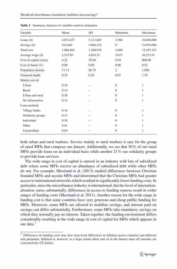
Summary statistics of the variables used in the scope estimation are in Table 1.6 Ofour rated MFI observations, 76 % only extend loans while the remaining 24 % offerboth loans and mobilize savings, confirming that most MFIs still offer only credit.MFIs in the largest to date MFI dataset maintained by mixmarket show the samedistribution of lending-only and lending and deposit institutions. The average MFIhas about $4.1 million in loan portfolio outstanding, with a range from slightly morethan $3,500 to $34.6 million. The volume of savings (when offered) is $914,669 onaverage and the largest case is about $24 million. The average value of annual salariesis $5,516, the cost of capital (deposits and borrowed funds) is 8 %, and the ratio of non-labor operating expense to net-fixed assets is 4.2. The average value of the populationdensity in the country in which the MFIs operate is 71 people per square kilometer, andit varies from sparsely populated countries with 2 to very densely populated countrieswith 1,050 people per square kilometer. Financial depth is the ratio of money aggregateincluding currency, deposits and electronic currency (M3) over GDP and measuresthe level of financial development. It is 0.39 on average varying from 0.07 to 1.39.We see that 34 % of our MFIs serve urban markets only and an additional 38 % serve
5 For a detailed comparison of this with other available datasets see Mersland (2009).6 Distribution of MFIs by country is presented in the “Appendix”. Comparison with other publicly availabledata shows that these data have more observations from Latin America.
123
Should all microfinance institutions mobilize microsavings?
Table 1 Summary statistics of variables used in estimation
Variable Mean SD Minimum Maximum
Loans ($) 4,071,677 5,111,683 3,586 34,604,000
Savings ($) 914,669 3,060,310 0 23,954,000
Total cost 1,086,463 1,288,910 2,689 12,197,321
Average wage ($) 5,515.85 4,054.15 18.07 26,572.67
Cost of capital (ratio) 4.22 29.04 0.04 800.00
Cost of funds (%) 0.08 0.09 0.00 0.93
Population density 71.13 86.79 2 1,050
Financial depth 0.39 0.20 0.07 1.39
Market served
Urban 0.34 – 0 1
Rural 0.14 – 0 1
Urban and rural 0.38 – 0 1
No information 0.14 – 0 1
Loan methods
Village banks 0.16 – 0 1
Solidarity groups 0.21 – 0 1
Individual 0.58 – 0 1
Other 0.01 – 0 1
Unclassified 0.04 – 0 1
both urban and rural markets. Service mainly to rural markets is rare for the groupof rated MFIs that compose our dataset. Additionally, we see that 58 % of our ratedMFIs provide loans on an individual basis while another 21 % use solidarity groupsto provide loan services.
The wide range in cost of capital is natural in an industry with lots of subsidizeddebt where some MFIs receive an abundance of subsidized debt while other MFIsdo not. For example, Mersland et al. (2013) studied differences between Christianfounded MFIs and secular MFIs and determined that the Christian MFIs had greateraccess to international networks which resulted in significantly lower funding costs. Inparticular, since the microfinance industry is international, but the level of internation-alization varies substantially, differences in access to funding sources result in widerranges of funding costs (Mersland et al. 2011). Another reason for the wide range infunding cost is that some countries have very generous and cheap public funding forMFIs. Moreover, some MFIs are allowed to mobilize savings, and interest paid onsavings can differ substantially. Furthermore, some MFIs take mandatory savings onwhich they normally pay no interest. Taken together, the funding environment differsconsiderably resulting in the wide range in cost of capital for MFIs which appears inour data.7
7 Differences in funding costs may also stem from differences in inflation across countries and differentrisk premiums. Inflation is, however, to a large extent taken care of in the dataset since all amounts areconverted into US dollars.
123
M. S. Delgado et al.
It is the presence of MFIs with 0 savings that require us to eschew a traditional costfunction approach to estimating scope economies and, in addition, the fact that someMFIs have zero input costs for funding implies that we must include input prices intoour semiparametric smooth coefficient cost function in level form as well. The addedgenerality afforded by our approach is key for analyzing these types of datasets as adhoc approaches to dealing with zeros are unappealing in applied settings. Further, usinglevel input prices as opposed to logarithmic prices is consistent with the theoreticalcost function of Baumol et al. (1982).
Lastly, a natural concern one may have with our empirical results is that lending-only MFIs may self-select and this will drive the results on scope economies wedetail here. We assume that there is no endogenous process of selection into depositcollecting for lending-only MFIs. MFIs vary by size so even institutions capable ofcollecting deposits may operate as lending-only if the local laws do not permit depositcollection by (small) MFIs. Many countries have adopted MFI-specific regulationsallowing variations in lending and savings (so it is not necessarily the underlyingcost structure that determines if an MFI collects deposits). For example, for a largecross-country sample, Hartarska et al. (2013) report that 63 % of the deposit-takingMFIs and 14 % of the lending-only MFIs were subject to central banking regulation.Hartarska and Nadolnyak (2007) allow for regulatory status to be correlated with MFI-specific characteristics and estimate a Hausmann-Taylor model of MFI performancebut do not find a difference in outreach and sustainability by regulatory status. Ina consequent article, Cull et al. (2011) observe that MFIs in the same country facedifferent enforcement, and find that the stringency of the country prudential regulations(onsite visits and their frequency) do not affect financial results but affect the depth ofoutreach (poverty level of clients). Numerous other studies have found that regulation(presumably of mainly deposit-taking institutions) does not affect performance, andprevious studies on the presence of scope economies for MFIs have assumed thatthere is no endogenous selection into deposit-taking MFIs (Mersland and Strøm 2009;Hartarska et al. 2010, 2011, 2013).
6 Results
For the model discussed in the previous section, we estimate both a parametric costsetup using nonlinear least squares following Pulley and Braunstein (1992) and a semi-parametric smooth coefficient cost function with two outputs and two input prices.8
Input prices are scaled by the price of physical capital (price of capital ratio) to pro-duce two relative input prices to be used in each piece of the cost function: labor costsand financial costs. Total costs and loans and deposits are scaled by 1,000,000 and10,000,000, respectively. All results were computed using R (R Development CoreTeam 2008). Bandwidths and polynomial order for the semiparametric model wereselected simultaneously via cross-validation over scope, discussed previously, using
8 Since the cost function is homothetic in input prices, we can always normalize by one of the input prices.Thus, while we have three inputs, only two of them enter into our analysis.
123
Should all microfinance institutions mobilize microsavings?
Table 2 Scope economy measures summarized at the quartiles
Overall scope Diseconomies Economies
Q1 0.0342 (0.0447) −0.0046 (0.0154) 0.0430 (0.1184)
Q2 0.1476 (0.2203) −0.0030 (0.0148) 0.1568 (2.1859)
Q3 0.4253 (0.4294) −0.0017 (0.1145) 0.4353 (1.0951)
Standard errors for each estimate are given below in parentheses. Estimates obtained via nonlinear leastsquares estimation of the parametric cost function
5 multistarts.9 In addition to normalized input prices entering the unknown smoothcoefficients, we also included the year in which the MFI was observed and its region(see “Appendix” for country and region classifications), as well as the main type oflending methodology the MFI uses (village bank, solidarity group, individual loan),the main market the MFI services (urban, rural or both), the population density of thearea in which the MFI operates, and the level of financial depth of the country. Givenour ability to smooth discrete variables, year, loan methodology and main marketserved were all smoothed using discrete kernels (see Li and Racine 2007).
6.1 Parametric cost function
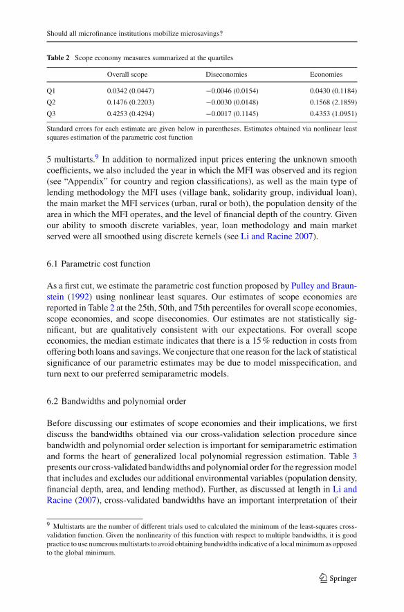
As a first cut, we estimate the parametric cost function proposed by Pulley and Braun-stein (1992) using nonlinear least squares. Our estimates of scope economies arereported in Table 2 at the 25th, 50th, and 75th percentiles for overall scope economies,scope economies, and scope diseconomies. Our estimates are not statistically sig-nificant, but are qualitatively consistent with our expectations. For overall scopeeconomies, the median estimate indicates that there is a 15 % reduction in costs fromoffering both loans and savings. We conjecture that one reason for the lack of statisticalsignificance of our parametric estimates may be due to model misspecification, andturn next to our preferred semiparametric models.
6.2 Bandwidths and polynomial order
Before discussing our estimates of scope economies and their implications, we firstdiscuss the bandwidths obtained via our cross-validation selection procedure sincebandwidth and polynomial order selection is important for semiparametric estimationand forms the heart of generalized local polynomial regression estimation. Table 3presents our cross-validated bandwidths and polynomial order for the regression modelthat includes and excludes our additional environmental variables (population density,financial depth, area, and lending method). Further, as discussed at length in Li andRacine (2007), cross-validated bandwidths have an important interpretation of their
9 Multistarts are the number of different trials used to calculated the minimum of the least-squares cross-validation function. Given the nonlinearity of this function with respect to multiple bandwidths, it is goodpractice to use numerous multistarts to avoid obtaining bandwidths indicative of a local minimum as opposedto the global minimum.
123
M. S. Delgado et al.
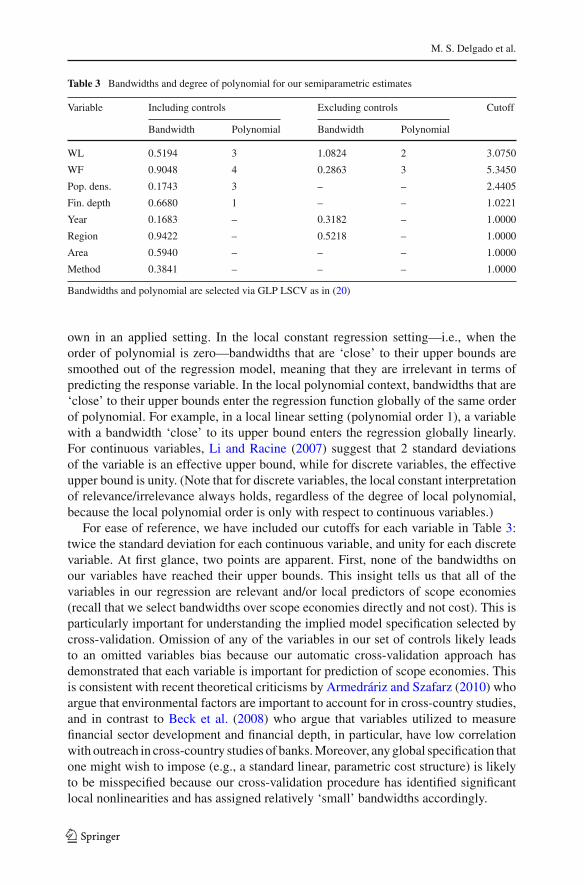
Table 3 Bandwidths and degree of polynomial for our semiparametric estimates
Variable Including controls Excluding controls Cutoff
Bandwidth Polynomial Bandwidth Polynomial
WL 0.5194 3 1.0824 2 3.0750
WF 0.9048 4 0.2863 3 5.3450
Pop. dens. 0.1743 3 – – 2.4405
Fin. depth 0.6680 1 – – 1.0221
Year 0.1683 – 0.3182 – 1.0000
Region 0.9422 – 0.5218 – 1.0000
Area 0.5940 – – – 1.0000
Method 0.3841 – – – 1.0000
Bandwidths and polynomial are selected via GLP LSCV as in (20)
own in an applied setting. In the local constant regression setting—i.e., when theorder of polynomial is zero—bandwidths that are ‘close’ to their upper bounds aresmoothed out of the regression model, meaning that they are irrelevant in terms ofpredicting the response variable. In the local polynomial context, bandwidths that are‘close’ to their upper bounds enter the regression function globally of the same orderof polynomial. For example, in a local linear setting (polynomial order 1), a variablewith a bandwidth ‘close’ to its upper bound enters the regression globally linearly.For continuous variables, Li and Racine (2007) suggest that 2 standard deviationsof the variable is an effective upper bound, while for discrete variables, the effectiveupper bound is unity. (Note that for discrete variables, the local constant interpretationof relevance/irrelevance always holds, regardless of the degree of local polynomial,because the local polynomial order is only with respect to continuous variables.)
For ease of reference, we have included our cutoffs for each variable in Table 3:twice the standard deviation for each continuous variable, and unity for each discretevariable. At first glance, two points are apparent. First, none of the bandwidths onour variables have reached their upper bounds. This insight tells us that all of thevariables in our regression are relevant and/or local predictors of scope economies(recall that we select bandwidths over scope economies directly and not cost). This isparticularly important for understanding the implied model specification selected bycross-validation. Omission of any of the variables in our set of controls likely leadsto an omitted variables bias because our automatic cross-validation approach hasdemonstrated that each variable is important for prediction of scope economies. Thisis consistent with recent theoretical criticisms by Armedráriz and Szafarz (2010) whoargue that environmental factors are important to account for in cross-country studies,and in contrast to Beck et al. (2008) who argue that variables utilized to measurefinancial sector development and financial depth, in particular, have low correlationwith outreach in cross-country studies of banks. Moreover, any global specification thatone might wish to impose (e.g., a standard linear, parametric cost structure) is likelyto be misspecified because our cross-validation procedure has identified significantlocal nonlinearities and has assigned relatively ‘small’ bandwidths accordingly.
123
Should all microfinance institutions mobilize microsavings?
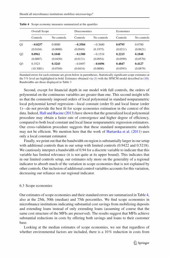
Table 4 Scope economy measures summarized at the quartiles
Overall Scope Diseconomies Economies
Controls No controls Controls No controls Controls No controls
Q1 −0.0257 0.0000 −0.3584 −0.3680 0.0795 0.0780
(0.0104) (0.0000) (0.0949) (0.1975) (0.0211) (0.0621)
Q2 0.0961 0.1040 −0.1300 −0.1534 0.2215 0.1848
(0.0007) (0.0450) (0.0131) (0.0954) (0.0599) (0.0570)
Q3 0.3523 0.3243 −0.0497 −0.0496 0.4847 0.4127
(10.3081) (0.0769) (0.0434) (0.0000) (0.0593) (0.0879)
Standard errors for each estimate are given below in parentheses. Statistically significant scope estimates atthe 5 % level are highlighted in bold. Estimates obtained via (1) with the SPSCM model described in (10).Bandwidths are those displayed in Table 3
Second, except for financial depth in our model with full controls, the orders ofpolynomial on the continuous variables are greater than one. This second insight tellsus that the commonly imposed orders of local polynomial in standard nonparametriclocal polynomial kernel regression—local constant (order 0) and local linear (order1)—do not provide the best fit for scope economies estimation in the context of thisdata. Indeed, Hall and Racine (2013) have shown that the generalized local polynomialprocedure may obtain a faster rate of convergence and higher degree of efficiency,compared to both local constant and local linear nonparametric regression estimators.Our cross-validation procedure suggests that these standard nonparametric modelsmay not be efficient. We mention here that the work of Hartarska et al. (2011) usesonly a local constant estimator.
Finally, we point out that the bandwidth on region is substantially larger in our setupwith additional controls than in our setup with limited controls (0.9422 and 0.5218).We cautiously interpret a bandwidth of 0.94 for a discrete variable to indicate that thisvariable has limited relevance (it is not quite at its upper bound). This indicates thatin our limited controls setup, our estimates rely more on the generality of a regionalindicator to absorb much of the variation in scope economies that is not explained byother controls. Our inclusion of additional control variables accounts for this variation,decreasing our reliance on our regional indicator.
6.3 Scope economies
Our estimates of scope economies and their standard errors are summarized in Table 4,also at the 25th, 50th (median) and 75th percentiles. We find scope economies inmicrofinance institutions indicating substantial cost savings from mobilizing depositsand extending loans instead of only extending loans (assuming of course that thesame cost structure of the MFIs are preserved). The results suggest that MFIs achievesubstantial reductions in costs by offering both savings and loans to their customerbase.
Looking at the median estimates of scope economies, we see that regardless ofwhether environmental factors are included, there is a 10 % reduction in costs from
123
M. S. Delgado et al.
offering both loans and savings. We find that there is not much difference in scopeestimates at the quartiles across both controls and limited controls specifications. Wefind that inclusion of our controls leads to a negative estimate of scope at the lowerquartile, and a slightly higher estimate at the upper quartile. We find that in bothmodels, scope economies are generally statistically significant at a 5 % confidencelevel. Furthermore, it is apparent that our estimates of scope are more heterogeneousin the model with full set of controls. These results indicate that there is heterogeneityinduced by our additional set of control variables.
Focusing on scope diseconomies, we see that the MFIs with estimated scope dis-economies have slightly lower levels of diseconomies when we account for our envi-ronmental controls. The median estimated scope diseconomies is −0.13, while themedian scope diseconomies for our model without controls is −0.15. The interquartilerange is slightly smaller. In general, however, these differences across set of controlsare not large enough to statistically distinguish between scope diseconomies in eachmodel. Notice that for our diseconomies estimates, we do not find as much statisti-cal significance in the model excluding our additional controls as in the full controlsspecification.10
Considering only those MFIs with scope economies, we see that our summary mea-sures are higher in the model with controls than our model without controls. Further,we find significance at each reported quartile, while our estimates without full controlsare only significant at the 50th and 75th percentiles. The statistical significance, as wellas relatively larger magnitude of scope economies estimates in the full controls modelsuggest that our control variables have a strong influence on the scope economies ofMFIs; such heterogeneity we explore in the following subsections.
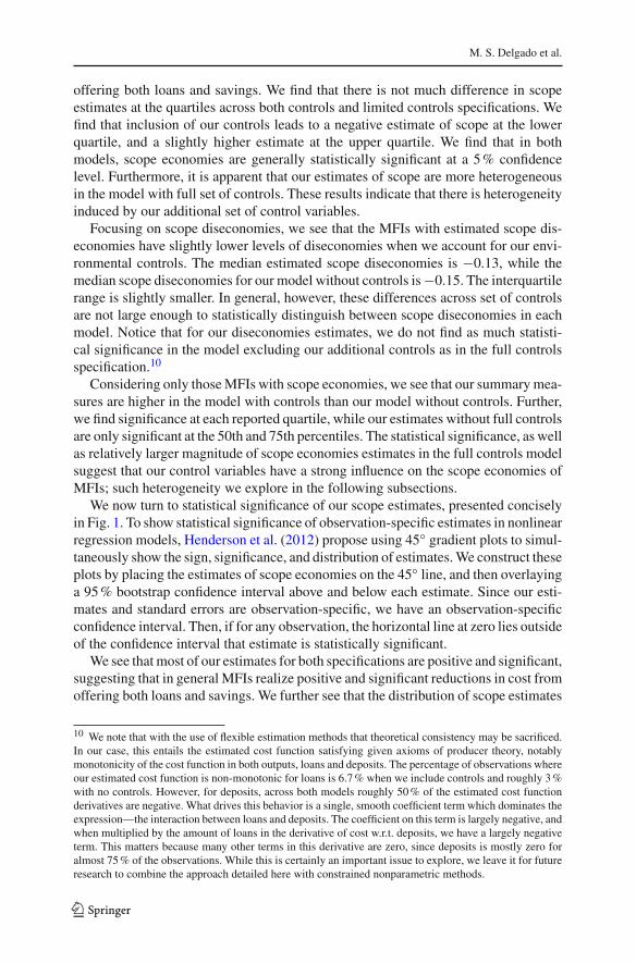
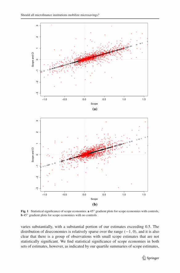
We now turn to statistical significance of our scope estimates, presented conciselyin Fig. 1. To show statistical significance of observation-specific estimates in nonlinearregression models, Henderson et al. (2012) propose using 45◦ gradient plots to simul-taneously show the sign, significance, and distribution of estimates. We construct theseplots by placing the estimates of scope economies on the 45◦ line, and then overlayinga 95 % bootstrap confidence interval above and below each estimate. Since our esti-mates and standard errors are observation-specific, we have an observation-specificconfidence interval. Then, if for any observation, the horizontal line at zero lies outsideof the confidence interval that estimate is statistically significant.
We see that most of our estimates for both specifications are positive and significant,suggesting that in general MFIs realize positive and significant reductions in cost fromoffering both loans and savings. We further see that the distribution of scope estimates
10 We note that with the use of flexible estimation methods that theoretical consistency may be sacrificed.In our case, this entails the estimated cost function satisfying given axioms of producer theory, notablymonotonicity of the cost function in both outputs, loans and deposits. The percentage of observations whereour estimated cost function is non-monotonic for loans is 6.7 % when we include controls and roughly 3 %with no controls. However, for deposits, across both models roughly 50 % of the estimated cost functionderivatives are negative. What drives this behavior is a single, smooth coefficient term which dominates theexpression—the interaction between loans and deposits. The coefficient on this term is largely negative, andwhen multiplied by the amount of loans in the derivative of cost w.r.t. deposits, we have a largely negativeterm. This matters because many other terms in this derivative are zero, since deposits is mostly zero foralmost 75 % of the observations. While this is certainly an important issue to explore, we leave it for futureresearch to combine the approach detailed here with constrained nonparametric methods.
123
Should all microfinance institutions mobilize microsavings?
(a)
(b)
Fig. 1 Statistical significance of scope economies. a 45◦ gradient plots for scope economies with controls,b 45◦ gradient plots for scope economies with no controls
varies substantially, with a substantial portion of our estimates exceeding 0.5. Thedistribution of diseconomies is relatively sparse over the range (−1, 0), and it is alsoclear that there is a group of observations with small scope estimates that are notstatistically significant. We find statistical significance of scope economies in bothsets of estimates, however, as indicated by our quartile summaries of scope estimates,
123
M. S. Delgado et al.
Table 5 Summary of scope economies by output structure at each quartile
Including controls Excluding controls
Loans Savings and loans Loans Savings and loans
Q1 −0.0270 −0.0246 0.0000 −0.0037
(0.0007) (0.0045) (0.0000) (0.0501)
Q2 0.0881 0.1353 0.0929 0.1800
(0.0003) (0.0301) (0.1438) (0.1073)
Q3 0.3166 0.4744 0.2611 0.5332
(0.0275) (0.1350) (0.1856) (0.4209)
Standard errors given below each estimate. Statistically significant estimates at the 5 % level are highlightedin bold
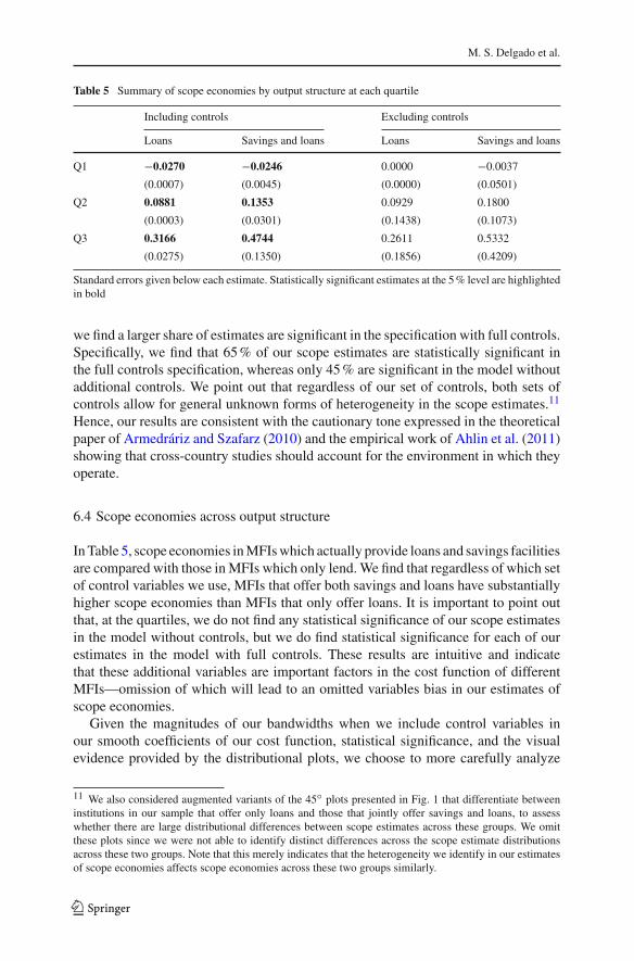
we find a larger share of estimates are significant in the specification with full controls.Specifically, we find that 65 % of our scope estimates are statistically significant inthe full controls specification, whereas only 45 % are significant in the model withoutadditional controls. We point out that regardless of our set of controls, both sets ofcontrols allow for general unknown forms of heterogeneity in the scope estimates.11
Hence, our results are consistent with the cautionary tone expressed in the theoreticalpaper of Armedráriz and Szafarz (2010) and the empirical work of Ahlin et al. (2011)showing that cross-country studies should account for the environment in which theyoperate.
6.4 Scope economies across output structure
In Table 5, scope economies in MFIs which actually provide loans and savings facilitiesare compared with those in MFIs which only lend. We find that regardless of which setof control variables we use, MFIs that offer both savings and loans have substantiallyhigher scope economies than MFIs that only offer loans. It is important to point outthat, at the quartiles, we do not find any statistical significance of our scope estimatesin the model without controls, but we do find statistical significance for each of ourestimates in the model with full controls. These results are intuitive and indicatethat these additional variables are important factors in the cost function of differentMFIs—omission of which will lead to an omitted variables bias in our estimates ofscope economies.
Given the magnitudes of our bandwidths when we include control variables inour smooth coefficients of our cost function, statistical significance, and the visualevidence provided by the distributional plots, we choose to more carefully analyze
11 We also considered augmented variants of the 45◦ plots presented in Fig. 1 that differentiate betweeninstitutions in our sample that offer only loans and those that jointly offer savings and loans, to assesswhether there are large distributional differences between scope estimates across these groups. We omitthese plots since we were not able to identify distinct differences across the scope estimate distributionsacross these two groups. Note that this merely indicates that the heterogeneity we identify in our estimatesof scope economies affects scope economies across these two groups similarly.
123
Should all microfinance institutions mobilize microsavings?
Table 6 Scope economy measures across regions, summarized at the quartiles
ECA LA SSA SEA MENA
Q1 −0.0325 −0.0592 0.0519 0.0615 −0.0287
(0.0007) (0.0238) (0.0764) (0.0076) (0.0078)
Q2 0.0795 0.0772 0.2409 0.2958 0.0315
(0.0211) (0.0524) (0.0516) (0.0609) (0.0052)
Q3 0.2648 0.3056 0.7005 0.6333 0.2334
(0.0305) (0.0402) (0.0111) (0.0270) (0.0539)
Standard errors for each estimate are below in parentheses; statistical significance at the 5 % level arehighlighted in bold
scope economies estimated via inclusion of these variables directly into the smoothcoefficients. All three of our key discrete variables—region, area and lending method—are not smoothed out of our model and therefore suggest an impact on the smoothcoefficients of our cost function and consequently our estimates of scope economies.
6.5 Scope economies across control variables
Given the fact that nonparametric models deliver estimates which are observation-specific, an intuitive way to present results is to condition on specific levels of thevariables of interest. To that end, we present our estimates of scope economies hereby focusing on how they vary across three of our most important controls, the regionthe MFI is located, the area in which the MFI provides services, and the type of loanstructure the MFI uses.
Scope economies are larger in countries with higher population density. For exam-ple, countries with scope diseconomies have average population densities of 47 personsper square km, while it is 81 persons per square km in countries with scope economies.This result seems to suggest that MFI’s working in less densely populated countrieswill have (or experience) diseconomies of scope. Here, MFIs may not have a con-sumer base large enough to provide savings accounts as well as lending opportunities.Recall, the presence of scope economies is such that cost sharing is available to theMFI via a product mix. In this case, it could turn out that MFIs in rural areas are notable to experience these cost-sharing opportunities the way that MFIs in more urbanand population dense areas are.
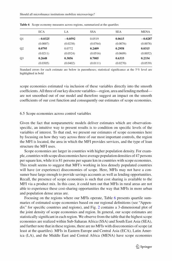
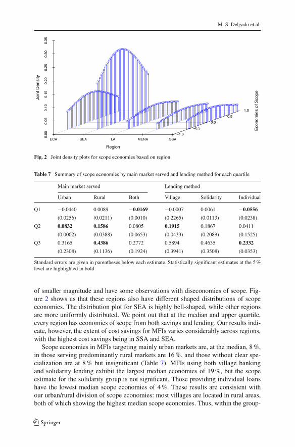
Focusing on the regions where our MFIs operate, Table 6 presents quartile sum-maries of estimated scope economies based on our regional definitions (see “Appen-dix” for specific countries and regions), and Fig. 2 contains a 3-dimensional plot ofthe joint density of scope economies and region. In general, our scope estimates arestatistically significant in each region. We observe from the table that the highest scopeeconomies are realized within Sub-Saharan Africa (SSA) and South East Asia (SEA),and further note that in these regions, there are no MFIs with diseconomies of scope (atleast at the quartiles). MFIs in Eastern Europe and Central Asia (ECA), Latin Amer-ica (LA), and the Middle East and Central Africa (MENA) have scope economies
123
M. S. Delgado et al.
Fig. 2 Joint density plots for scope economies based on region
Table 7 Summary of scope economies by main market served and lending method for each quartile
Main market served Lending method
Urban Rural Both Village Solidarity Individual
Q1 −0.0440 0.0089 −0.0169 −0.0007 0.0061 −0.0556
(0.0256) (0.0211) (0.0010) (0.2265) (0.0113) (0.0238)
Q2 0.0832 0.1586 0.0805 0.1915 0.1867 0.0411
(0.0002) (0.0388) (0.0653) (0.0433) (0.2089) (0.1525)
Q3 0.3165 0.4386 0.2772 0.5894 0.4635 0.2332
(0.2308) (0.1136) (0.1924) (0.3941) (0.3508) (0.0353)
Standard errors are given in parentheses below each estimate. Statistically significant estimates at the 5 %level are highlighted in bold
of smaller magnitude and have some observations with diseconomies of scope. Fig-ure 2 shows us that these regions also have different shaped distributions of scopeeconomies. The distribution plot for SEA is highly bell-shaped, while other regionsare more uniformly distributed. We point out that at the median and upper quartile,every region has economies of scope from both savings and lending. Our results indi-cate, however, the extent of cost savings for MFIs varies considerably across regions,with the highest cost savings being in SSA and SEA.
Scope economies in MFIs targeting mainly urban markets are, at the median, 8 %,in those serving predominantly rural markets are 16 %, and those without clear spe-cialization are at 8 % but insignificant (Table 7). MFIs using both village bankingand solidarity lending exhibit the largest median economies of 19 %, but the scopeestimate for the solidarity group is not significant. Those providing individual loanshave the lowest median scope economies of 4 %. These results are consistent withour urban/rural division of scope economies: most villages are located in rural areas,both of which showing the highest median scope economies. Thus, within the group-
123
Should all microfinance institutions mobilize microsavings?
(a)
(b)
Fig. 3 Boxplots for scope economies based on service area and loan method. a Scope economies by servicearea. b Scope economies by loan method
lending methodologies, village banks are more likely to be cost effective in mobilizingdeposits. We believe this is because in village banking the MFI has a captured audiencewith whom credit officers can relate to and understand.
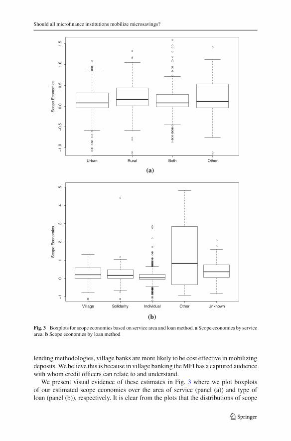
We present visual evidence of these estimates in Fig. 3 where we plot boxplotsof our estimated scope economies over the area of service (panel (a)) and type ofloan (panel (b)), respectively. It is clear from the plots that the distributions of scope
123
M. S. Delgado et al.
estimates over each of these different groups varies substantially; not only do thesedistributions have different central tendencies and interquartile ranges, it is clear thatseveral of these distributions are asymmetric. The top panel in the figure shows thatthe rural areas generally have a higher estimate of scope economies, as does the villagebanking group in the bottom panel.
6.6 Quasi economies of scope
So far, our analysis has focused on the standard scope economies estimate based onEq. (1). As pointed out by Pulley and Braunstein (1992), this measure assumes thateach firm perfectly specializes, which may not be reflected empirically by the data.As a robustness check of our primary scope estimates, we focus on the subsampleof firms in our dataset (178 observations) that jointly produce both savings and loansand estimate quasi economies of scope defined in Eq. (2).12 We follow our earliereconometric strategy and deploy the generalized local polynomial estimator for thesmooth coefficient cost function, with bandwidths selected by smoothing over quasiscope. We assume the degree of specialization of each firm is (1 − ε) = 0.85.
Our restricted sample of microfinance institutions of 178 observations renders semi-parametric estimation with the full set of environmental variables infeasible becauseof dimensionality issues relative to the small sample size. We therefore focus on therestricted set of environmental controls, namely the cost of labor and financial cap-ital inputs, year and region. Before reporting summaries of our estimates of quasieconomies of scope, we report that our bandwidths on each of our nonparametricvariables lie below their respective upper bounds, indicating that each variable is bothrelevant and a nonlinear predictor of heterogeneity in the cost coefficient functions.Further, our generalized local polynomial optimization results indicate that the optimalorder of local polynomial for both continuously distributed nonparametric environ-mental variables is of order 3. As in our scope economies estimates, we find evidencethat the standard local constant or local linear estimators are not of optimal polynomialorder for constructing our estimate of quasi-scope economies.
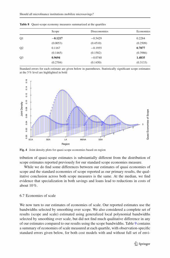
Table 8 reports quartile summaries of the quasi economies of scope estimates. Wesee that our estimates of quasi economies of scope are slightly larger in magnitudethan our estimates of scope economies reported previously, with a median effect ofapproximately 0.12. It is apparent, however, that the upper quartile of quasi-scope issubstantially higher than for scope. This suggests that the distribution of quasi-scopeeconomies is left skewed. Notice that while we find some evidence of diseconomiesof scope for a subset of observations, none of these diseconomies estimates are statis-tically significant at any of the reported quartiles of diseconomies of scope.
Figure 4 shows the joint density plot between regions and quasi economies ofscope. We see that the distribution of quasi economies of scope is indeed left skewed,as suggested by the quartiles reported in Table 8. Notice that this skewed shaped dis-
12 As a comparison, we consider our standard scope measure for only this subset of 178 countries and findthat, while there is a wider interquartile range of our estimates, the qualitative conclusion from our mainresults is unchanged.
123
Should all microfinance institutions mobilize microsavings?
Table 8 Quasi-scope economy measures summarized at the quartiles
Scope Diseconomies Economies
Q1 −0.1217 −0.5429 0.2284
(0.0053) (0.4510) (0.2509)
Q2 0.1167 −0.1955 0.7877
(0.1465) (0.1582) (0.3986)
Q3 0.9694 −0.0740 1.4835
(0.2704) (0.1450) (0.3133)
Standard errors for each estimate are given below in parentheses. Statistically significant scope estimatesat the 5 % level are highlighted in bold
Fig. 4 Joint density plots for quasi-scope economies based on region
tribution of quasi-scope estimates is substantially different from the distribution ofscope estimates reported previously for our standard scope economies measure.
While we do find some differences between our estimates of quasi economies ofscope and the standard economies of scope reported as our primary results, the qual-itative conclusion across both scope measures is the same. At the median, we findevidence that specialization in both savings and loans lead to reductions in costs ofabout 10 %.
6.7 Economies of scale
We now turn to our estimates of economies of scale. Our reported estimates use thebandwidths selected by smoothing over scope. We also considered a complete set ofresults (scope and scale) estimated using generalized local polynomial bandwidthsselected by smoothing over scale, but did not find much qualitative difference in anyof our estimates compared to our results using the scope bandwidths. Table 9 containsa summary of economies of scale measured at each quartile, with observation-specificstandard errors given below, for both cost models with and without full set of envi-
123
M. S. Delgado et al.
Table 9 Scale economy measures summarized at the quartiles
Overall scale Diseconomies Economies
Controls No controls Controls No controls Controls No controls
Q1 0.5164 0.7666 0.3373 0.4654 1.2747 1.1923
(0.0601) (0.2317) (0.1980) (0.3022) (0.1610) (0.3353)
Q2 0.8940 1.0585 0.5584 0.7319 1.7627 1.4886
(0.0172) (1.0355) (0.0660) (0.5207) (0.1084) (0.2594)
Q3 1.5928 1.5684 0.7690 0.8660 2.8881 2.2047
(0.1308) (0.1523) (0.0159) (0.1969) (0.0090) (2.9465)
Standard errors for each estimate are given below in parentheses. Statistically significant scale estimates atthe 5 % level are highlighted in bold
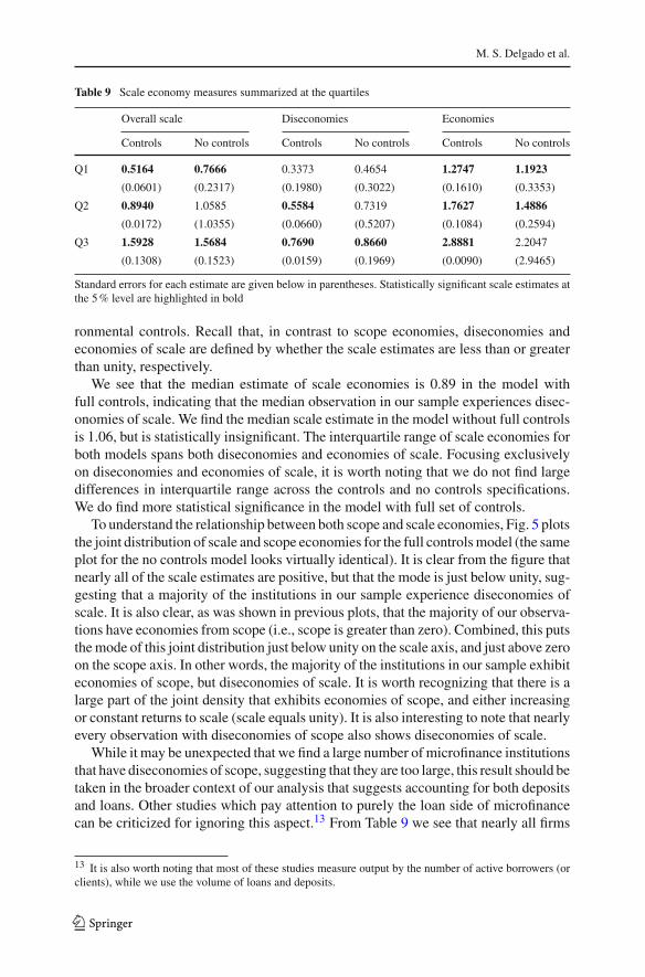
ronmental controls. Recall that, in contrast to scope economies, diseconomies andeconomies of scale are defined by whether the scale estimates are less than or greaterthan unity, respectively.
We see that the median estimate of scale economies is 0.89 in the model withfull controls, indicating that the median observation in our sample experiences disec-onomies of scale. We find the median scale estimate in the model without full controlsis 1.06, but is statistically insignificant. The interquartile range of scale economies forboth models spans both diseconomies and economies of scale. Focusing exclusivelyon diseconomies and economies of scale, it is worth noting that we do not find largedifferences in interquartile range across the controls and no controls specifications.We do find more statistical significance in the model with full set of controls.
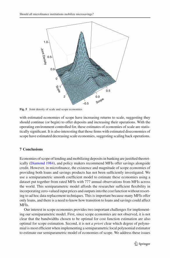
To understand the relationship between both scope and scale economies, Fig. 5 plotsthe joint distribution of scale and scope economies for the full controls model (the sameplot for the no controls model looks virtually identical). It is clear from the figure thatnearly all of the scale estimates are positive, but that the mode is just below unity, sug-gesting that a majority of the institutions in our sample experience diseconomies ofscale. It is also clear, as was shown in previous plots, that the majority of our observa-tions have economies from scope (i.e., scope is greater than zero). Combined, this putsthe mode of this joint distribution just below unity on the scale axis, and just above zeroon the scope axis. In other words, the majority of the institutions in our sample exhibiteconomies of scope, but diseconomies of scale. It is worth recognizing that there is alarge part of the joint density that exhibits economies of scope, and either increasingor constant returns to scale (scale equals unity). It is also interesting to note that nearlyevery observation with diseconomies of scope also shows diseconomies of scale.
While it may be unexpected that we find a large number of microfinance institutionsthat have diseconomies of scope, suggesting that they are too large, this result should betaken in the broader context of our analysis that suggests accounting for both depositsand loans. Other studies which pay attention to purely the loan side of microfinancecan be criticized for ignoring this aspect.13 From Table 9 we see that nearly all firms
13 It is also worth noting that most of these studies measure output by the number of active borrowers (orclients), while we use the volume of loans and deposits.
123
Should all microfinance institutions mobilize microsavings?
Fig. 5 Joint density of scale and scope economies
with estimated economies of scope have increasing returns to scale, suggesting theyshould continue (or begin) to offer deposits and increasing their operations. With theoperating environment controlled for, these estimates of economies of scale are statis-tically significant. It is also interesting that those firms with estimated diseconomies ofscope have estimated decreasing scale economies, suggesting scaling back operations.
7 Conclusions
Economies of scope of lending and mobilizing deposits in banking are justified theoret-ically (Diamond 1984), and policy makers recommend MFIs offer savings alongsidecredit. However, in microfinance, the existence and magnitude of scope economies ofproviding both loans and savings products has not been sufficiently investigated. Weuse a semiparametric smooth coefficient model to estimate these economies using adataset put together from rated MFIs with 777 annual observations from MFIs acrossthe world. This semiparametric model affords the researcher sufficient flexibility inincorporating zero-valued input prices and outputs into the cost function without resort-ing to ad hoc data replacement techniques. This is important because many MFIs offeronly loans, and there is a need to know how transition to loans and savings could affectMFIs.
Our interest in scope economies provides two important challenges for implement-ing our semiparametric model. First, since scope economies are not observed, it is notclear that the bandwidths chosen to be optimal for cost function estimation are alsooptimal for scope estimation. Second, it is not a priori clear which degree of polyno-mial is most efficient when implementing a semiparametric local polynomial estimatorto estimate our semiparametric model of economies of scope. We address these issues
123
M. S. Delgado et al.
simultaneously by combining two novel econometric approaches: a generalized localpolynomial estimator that allows both the bandwidth and degree of polynomial to beselected via data-driven cross-validation, and a cross-validation method that allowsfor bandwidth selection over an unobserved measurement. We point out that (i) neitherof these methods have been used empirically; (ii) these methods have never been usedsimultaneously; and (iii) these methods have never been considered in a semiparamet-ric regression context.
We estimate two models of scope economies, one where only variables typ-ically used in a cost function approach are included (total cost, output values,and relative input prices) and a model where in addition to these variables weinclude population density, a measure of financial sector development, type of mar-ket served (urban, rural or both), and the predominant loan methodology (villagebanking, solidarity groups and individual loans), as well as controls for time andregion. We find that scope economies are substantial across both settings and,for either model, that most of the MFIs in our dataset have (or would) experi-ence reductions in cost by offering both savings and loan services. We find thatour estimates of scope economies are generally more significant when we includethe full set of environmental variables, and that while most of our observationsexhibit economies of scope, the modal observation also exhibits diseconomies ofscale.
Overall, our finding of scope economies is intuitive and relevant. In tumultuousfinancial markets, the finding that MFIs mobilizing local savings may not only pro-vide much needed services for the poor but may also have cost advantages is impor-tant. This suggests that agencies providing funding to MFIs could encourage bothmicrosavings and microloan services be offered. This requires increased attention oncreating a regulatory environment allowing MFIs to accept deposits, or strengtheningthe MFI and maybe even donor support for them to become licensed deposit mobi-lizing institutions. However, since around 25 % of MFIs experience diseconomies ofscope, largely stemming from environmental factors, the implication for policy mak-ers is that general recommendations should be avoided. More research is needed tounderstand microfinance regulations, the costs and benefits involved and what type ofregulation is actually needed for the mobilization of microsavings. For example, inthe environments where MFIs operate, could there be other governance mechanismsthat would protect the depositors as well as a public regulator? Future work on scopeeconomies in microfinance should attempt to obtain a more comprehensive data setfor MFIs and determine if other environmental variables are relevant in MFIs’ coststructures.
Appendix
Distribution of MFIs by country is presented in Table 10. Comparison with other pub-licly available data shows that these data have more observations from Latin America,perhaps because they needed external funds.
123
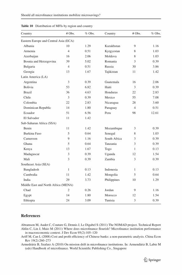
Should all microfinance institutions mobilize microsavings?
Table 10 Distribution of MFIs by region and country
Country # Obs. % Obs. Country # Obs. % Obs.
Eastern Europe and Central Asia (ECA)
Albania 10 1.29 Kazakhstan 9 1.16
Armenia 4 0.51 Kyrgyzstan 8 1.03
Azerbaijan 16 2.06 Moldova 8 1.03
Bosnia and Herzegovina 39 5.02 Romania 3 0.39
Bulgaria 4 0.51 Russia 30 3.86
Georgia 13 1.67 Tajikistan 11 1.42
Latin America (LA)
Argentina 3 0.39 Guatemala 16 2.06
Bolivia 53 6.82 Haiti 3 0.39
Brazil 36 4.63 Honduras 22 2.83
Chile 3 0.39 Mexico 55 7.08
Colombia 22 2.83 Nicaragua 28 3.60
Dominican Republic 14 1.80 Paraguay 4 0.51
Ecuador 51 6.56 Peru 98 12.61
El Salvador 11 1.42
Sub-Saharan Africa (SSA)
Benin 11 1.42 Mozambique 3 0.39
Burkina Faso 5 0.64 Senegal 8 1.03
Cameroon 9 1.16 South Africa 3 0.39
Ghana 5 0.64 Tanzania 3 0.39
Kenya 13 1.67 Togo 1 0.13
Madagascar 3 0.39 Uganda 12 1.54
Mali 3 0.39 Zambia 3 0.39
Southeast Asia (SEA)
Bangladesh 1 0.13 Indonesia 1 0.13
Cambodia 11 1.42 Mongolia 5 0.64
India 29 3.73 Philippines 10 1.29
Middle East and North Africa (MENA)
Chad 2 0.26 Jordan 9 1.16
Egypt 14 1.80 Morocco 12 1.54
Ethiopia 24 3.09 Tunisia 3 0.39
References
Abramson M, Audet C, Couture G, Dennis J, Le Digabel S (2011) The NOMAD project. Technical ReportAhlin C, Lin J, Maio M (2011) Where does microfinance flourish? Microfinance institution performance
in macroeconomic context. J Dev Econ 95(2):105–120Ariff M, Can L (2008) Cost and profit efficiency of Chinese banks: a non-parametric analysis. China Econ
Rev 19(2):260–273Armedráriz B, Szafarz A (2010) On mission drift in microfinance institutions. In: Armendáriz B, Labie M
(eds) Handbook of microfinance. World Scientific Publishing Co., Singapore
123
M. S. Delgado et al.
Balkenhol B (2009) Microfinance and public policy. Outreach, performance and efficiency. Palgrave, NewYork
Baumol WJ, Panzer J, Willig R (1982) Contestable markets and the theory of market structure. Harcourt,New York
Beck T, Demirguc-Kunt A, Martinez P, Soledad M (2008) Symposium on access to finance: banking servicesfor everyone? Barriers to bank access and use around the world. World Bank Econ Rev 22(3):397–430
Berger A, Humphrey D (1991) The dominance of inefficiences over scale and product mix economies inbanking. J Monet Econ 28:117–148
Berger AN, Hasan I, Zhou M (2009) Bank ownership and efficiency in China: what will happen in theworlds largest nation? J Bank Financ 33:113–130
Caudill SB, Gropper DM, Hartarska V (2009) Which microfinance institutions are becoming more costeffective with time? Evidence from a mixture model. J Money Credit Bank 41:651–672
Christiansen LR, Jorgensen DW, Lau LJ (1971) Conjugate duality and the transcendental logarithmicproduction function. Econometrica 39:255–256
Collins D, Morduch J, Rutherford S, Ruthven O (2009) Portfolios of the poor: how the world’s poor liveon $2 a day. Princeton University Press, New Jersey
Cull R, Demirguc-Kunt A, Morduch J (2007) Financial performance and outreach a global analysis ofleading MFIs. Econ J 117:F107–F133
Cull R, Demirguc-Kunt A, Morduch J (2009) Microfinance meets the market. J Econ Perspect 23:167–192Cull R, Demirguc-Kunt A, Morduch J (2011) Does regulatory supervision curtail microfinance profitability
and outreach? World Dev 39:949–965Diamond D (1984) Financial intermediation and delegated monitoring. Rev Econ Stud 51:393–414Du P, Parmeter CF, Racine JS (2013) Nonparametric kernel regression with multiple predictors and multiple
shape constraints. Stat Sin 23:1343–1372Freixas X, Rochet J (1997) Microeconomics of banking. MIT Press, CambridgeGarmaise MJ, Natividad G (2010) Information, the cost of credit, and operational efficiency: an empirical
study of microfinance. Rev Financ Stud 23:2560–2590Gutierres-Nieto B, Serrano-Cinca C, Mar M (2007) Microfinance institutions and efficiency. Omega Int J
Manag Sci 35:131–142Hall PG, Racine JS (2013) Infinite order cross-validated local polynomial regression. Working paperHartarska V, Mersland R (2012) What governance mechanisms promote efficiency in reaching poor clients?
Evidence from rated microfinance institutions. Eur Financ Manag 18:218–239Hartarska V, Mersland R, Nadolnyak D, Parmeter CF (2013) Governance and scope economies in microfi-
nance institutions. Int J Corp Gov 4(1):74–96Hartarska V, Nadolnyak D (2007) Do regulated microfinance institutions achieve better sustainability and
outreach? Cross-country evidence. Appl Econ 39(10–12):1207–1222Hartarska V, Parmeter CF, Nadolnyak D (2011) Economies of scope of lending and mobilizing deposits in
microfinance institutions: a semiparametric analysis. Am J Agric Econ 93(2):389–398Hartarska V, Parmeter CF, Nadolnyak D, Zhou B (2010) Economics of scope for microfinance: differences
across output measures. Pac Econ Rev 15(4):464–481Hartarska V, Shen X, Mersland R (2013) Scale economies and elasticities of substitution in microfinance
instituitions. J Bank Financ 37:118–131Henderson DJ, Kumbhakar SC, Parmeter CF (2012) A simple method to visualize results in nonlinear
regression models. Econ Lett 117:578–581Henderson DJ, List JA, Millimet DL, Parmeter CF, Price MK (2012) Empirical implementation of non-
parametric first-price auction models. J Econom 168:17–28Hermes N, Lensink B, Meesters A (2011) Outreach and efficiency of microfinance institutions. World Dev
39:938–948Hughes JP, Mester L (2009) Efficiency in banking: theory, practice, and evidence, Chapter 19. In: Berger
AN, Molyneux P, Wilson J (eds) The Oxford handbook of banking. Oxford University Press, OxfordHumphrey DB (1985) Costs and scale economies in bank intermediation. In: Aspinwail RC, Eisenbeis RA
(eds) Handbook for banking strategy. Wiley, New YorkLi Q, Racine J (2007) Nonparametric econometrics: theory and practice. Princeton University Press, Prince-
tonMersland R (2009) Corporate governance and ownership in microfinance organizations. PhD thesis, Uni-
versity of Agder
123
Should all microfinance institutions mobilize microsavings?
Mersland R, D’Espallier B, Supphellen M (2013) The effect of religion on development efforts: evidencefrom the microfinance industry and a research agenda. World Dev 41(1):145–156
Mersland R, Randøy T, Strøm RØ (2011) The impact of international influence on microbanks performance:a global survey. Int Bus Rev 20(2):163–176
Mersland R, Strøm RØ (2009) Performance and governance in microfinance institutions. J Bank Financ33(4):662–669
Mitchell K, Onvural NM (1996) Economies of scale and scope at large commercial banks: evidence fromthe Fourier flexible functional form. J Money Credit Bank 28:178–199
Nie Z, Racine JS (2012) The crs package: nonparametric regression splines for continuous and categoricalpredictors. R Journal 4:48–56
Paxton J (2007) Technical efficiency in a semi-formal financial sector: the case of Mexico. Oxf Bull EconStat 69(1):57–74
Pulley LB, Braunstein YM (1992) A composite cost function for multiproduct firms with an application toeconomies of scope in banking. Rev Econ Stat 74:213–230
Pulley LB, Humphrey D (1993) The role of fixed costs and cost complementarities in determining scopeeconomies and the cost of narrow banking proposals. J Bus 66:437–462
R Development Core Team (2008) R: a language and environment for statistical computing. R Foundationfor Statistical Computing, Vienna, Austria. ISBN 3-900051-07-0
Racine JS, Li Q (2004) Nonparametric estimation of regression functions with both categorical and contin-uous data. J Econom 119(1):99–130
van Cayseele P, Wuyts C (2007) Cost efficiency in the European securities settlement and depositoryindustry. J Bank Financ 31(10):3058–3079
Varian H (1984) The nonparametric approach to production analysis. Econometrica 52(3):579–597
123