Embed Size (px)
Citation preview
Mathematical Principles of Theoretical Physics
Tian Ma
Shouhong Wang
March 30, 2015

2

To our families

ii
Preface
The objectives of this book are to derive experimentally verifiable laws of Nature based on
a few fundamental mathematical principles, and to provide new insights and solutions to a
number of challenging problems of theoretical physics. This book focuses mainly on the
symbiotic interplay between theoretical physics and advanced mathematics.
The great success and experimental verification of both Albert Einstein’s theory of rel-
ativity and quantum mechanics have placed them as cornerstones of modern physics. The
fundamental principles of both relativity and quantum mechanics are the starting point of the
study undertaken in this book.
James Clerk Maxwell’s discovery of the Maxwell equations marks the beginning of the
field theory and the gauge theory. The quantum electrodynamics (QED) is beautifully de-
scribed by the U(1) abelian gauge theory. The non-abelian SU(N) gauge theory was origi-
nated from the early work of (Weyl, 1919; Klein, 1938; Yang and Mills, 1954). Physically,
gauge invariance refers to the conservation of certain quantum property of the interacting
physical system. Such quantum property of N particles cannot be distinguished for the in-
teraction. Consequently, the energy contribution of these N particles associated with the
interaction is invariant under the general SU(N) phase (gauge) transformations.
The success and experimental support of the gauge theory in describing the electromag-
netism, the strong and the weak interactions clearly demonstrate that the principle of gauge
invariance is indeed a principle of Nature.
We have, at our disposal, the principle of general relativity, the principle of Lorentz invari-
ance (special theory of relativity), and the principle of gauge invariance. These are symmetry
principles. We can show that these symmetry principles, together with the simplicity of laws
of Nature, dictate the actions of the four fundamental interactions of Nature: the gravity, the
electromagnetism, the strong and the weak interactions.
Modern theoretical physics also faces great challenges and mysteries. For example, in
astrophysics and cosmology, the most important challenges and mysteries include 1) the un-
explained dark matter and dark energy phenomena, 2) the existence and properties of black
holes, 3) the structure and origin of our Universe, and 4) the mechanism of supernovae ex-
plosion and active galactic nucleus jets. In particles physics, the nature of Higgs fields, quark
confinement and the unification of four fundamental interactions are among the grand chal-
lenges.
The breakthrough of our work presented in this book and in a sequence of papers comes
from our recent discovery of three new fundamental principles: the principle of interac-
tion dynamics (PID), the principle of representation invariance (PRI) (Ma and Wang, 2014e,
iii
iv
2015a, 2014h), and the principle of symmetry-breaking (PSB) (Ma and Wang, 2014a).
Basically, PID takes the variation of the Lagrangian action under the energy-momentum
conservation constraints. For gravity, PID is the direct consequence of the presence of dark
energy and dark matter. For the weak interaction, PID is the requirement of the presence of
the Higgs field. For the strong interaction, we demonstrated that PID is the consequence of
the quark confinement phenomena.
PRI requires that the gauge theory be independent of the choices of the representation
generators. These representation generators play the same role as coordinates, and in this
sense, PRI is a coordinate-free invariance/covariance, reminiscent of the Einstein principle of
general relativity. In other words, PRI is purely a logic requirement for the gauge theory.
PSB offers an entirely different route of unification from the Einstein unification route
which uses large symmetry group. The three sets of symmetries — the general relativistic
invariance, the Lorentz and gauge invariances, as well as the Galileo invariance — are mu-
tually independent and dictate in part the physical laws in different levels of Nature. For a
system coupling different levels of physical laws, part of these symmetries must be broken.
These three new principles have profound physical consequences, and, in particular, pro-
vide a new route of unification for the four interactions:
1) the general relativity and the gauge symmetries dictate the Lagrangian;
2) the coupling of the four interactions is achieved through PID and PRI in
the unified field equations, which obey the PGR and PRI, but break sponta-
neously the gauge symmetry;
3) the unified field model can be easily decoupled to study individual interac-
tion, when the other interactions are negligible; and
4) the unified field model coupling the matter fields using PSB.
The main part of this book is to establish such a field theory, and to provide explanations
and solutions to a number of challenging problems and mysteries such as those mentioned
above.
Another part of the book is on building a phenomenological weakton model of elementary
particles, based on the new field theory that we established. This model explains all the
subatomic decays and scattering, and gives rise to new insights on the structure of subatomic
particles.
Our new field theory is based solely on a few fundamental principles. It agrees with all
the related experiments and observations, and solves many challenging problems in modern
physics. In this sense, it should reflect the truth of the Nature!
In retrospect, most attempts in modern physics regarding to the challenges and mysteries
mentioned earlier focus on modifying, on an ad hoc basis, the basic Lagrangian actions.
Even with careful tuning, these artificial modifications often lead to unsolvable difficulties
and confusions on model-building and on the understanding of the related phenomena. The
PID approach we discovered is the first principle approach, required by the phenomena as
the dark matter, dark energy, quark confinement, and the Higgs field. It leads to dual fields,
which are not achievable by other means. Hence we believe that this is the very reason behind
the confusions and challenges that modern physics has faced for many decades.
Chapter 1, General Introduction, is written for everyone. It synthesizes the main ideas
and results obtained in this book. Chapter 2 develops the general view and basic physical
v
backgrounds needed for later chapters. Chapter 3 provides the needed mathematical founda-
tions for PID, PRI and the geometry for the unified fields. More physical oriented readers can
jump directly to later chapters, Chapters 4-7, for the main physical developments.
The research presented in this book was supported in part by grants from the US NSF
and the Chinese NSF. The authors are most grateful for their advice, encouragement, and
consistent support from Louis Nirenberg, Roger Temam, and Wenyuan Chen throughout our
scientific career. Our warm thanks to Jie Shen, Mickael Chekroun, Xianling Fan, Kevin
Zumbrun, Wen Masters and Reza Malek-Madani for their support, insightful discussions and
appreciation for his work.
Last but not least, we would like to express our gratitude to our wives, Li and Ping, and
our children, Jiao, Melinda and Wayne, for their love and appreciation. In particular, we are
most grateful for Li and Ping’s unflinching support and understanding during the long course
of our academic career.
March 30, 2015
Chengdu, China Tian Ma
Bloomington, IN Shouhong Wang

vi
Contents
1 General Introduction 1
1.1 Challenges of Physics and Guiding Principle . . . . . . . . . . . . . . . . . . 1
1.2 Law of Gravity, Dark Matter and Dark Energy . . . . . . . . . . . . . . . . . 3
1.3 First Principles of Four Fundamental Interactions . . . . . . . . . . . . . . . 6
1.4 Symmetry and Symmetry-Breaking . . . . . . . . . . . . . . . . . . . . . . 11
1.5 Unified Field Theory Based On PID and PRI . . . . . . . . . . . . . . . . . 13
1.6 Theory of Strong Interactions . . . . . . . . . . . . . . . . . . . . . . . . . . 16
1.7 Theory of Weak Interactions . . . . . . . . . . . . . . . . . . . . . . . . . . 18
1.8 New Theory of Black Holes . . . . . . . . . . . . . . . . . . . . . . . . . . 19
1.9 The Universe . . . . . . . . . . . . . . . . . . . . . . . . . . . . . . . . . . 21
1.10 Supernovae Explosion and AGN Jets . . . . . . . . . . . . . . . . . . . . . . 25
1.11 Multi-Particle Systems and Unification . . . . . . . . . . . . . . . . . . . . . 26
1.12 Weakton Model of Elementary Particles . . . . . . . . . . . . . . . . . . . . 28
2 Fundamental Principles of Physics 33
2.1 Essence of Physics . . . . . . . . . . . . . . . . . . . . . . . . . . . . . . . 34
2.1.1 General guiding principles . . . . . . . . . . . . . . . . . . . . . . . 34
2.1.2 Phenomenological methods . . . . . . . . . . . . . . . . . . . . . . 35
2.1.3 Fundamental principles in physics . . . . . . . . . . . . . . . . . . . 36
2.1.4 Symmetry . . . . . . . . . . . . . . . . . . . . . . . . . . . . . . . . 38
2.1.5 Invariance and tensors . . . . . . . . . . . . . . . . . . . . . . . . . 39
2.1.6 Geometric interaction mechanism . . . . . . . . . . . . . . . . . . . 42
2.1.7 Principle of symmetry-breaking . . . . . . . . . . . . . . . . . . . . 44
2.2 Lorentz Invariance . . . . . . . . . . . . . . . . . . . . . . . . . . . . . . . 46
2.2.1 Lorentz transformation . . . . . . . . . . . . . . . . . . . . . . . . . 46
2.2.2 Minkowski space and Lorentz tensors . . . . . . . . . . . . . . . . . 47
2.2.3 Relativistic invariants . . . . . . . . . . . . . . . . . . . . . . . . . . 51
2.2.4 Relativistic mechanics . . . . . . . . . . . . . . . . . . . . . . . . . 52
2.2.5 Lorentz invariance of electromagnetism . . . . . . . . . . . . . . . . 54
2.2.6 Relativistic quantum mechanics . . . . . . . . . . . . . . . . . . . . 56
2.2.7 Dirac spinors . . . . . . . . . . . . . . . . . . . . . . . . . . . . . . 58
2.3 Einstein’s Theory of General Relativity . . . . . . . . . . . . . . . . . . . . 60
2.3.1 Principle of general relativity . . . . . . . . . . . . . . . . . . . . . . 60
2.3.2 Principle of equivalence . . . . . . . . . . . . . . . . . . . . . . . . 61
vii
viii CONTENTS
2.3.3 General tensors and covariant derivatives . . . . . . . . . . . . . . . 63
2.3.4 Einstein-Hilbert action . . . . . . . . . . . . . . . . . . . . . . . . . 67
2.3.5 Einstein gravitational field equations . . . . . . . . . . . . . . . . . . 68
2.4 Gauge Invariance . . . . . . . . . . . . . . . . . . . . . . . . . . . . . . . . 70
2.4.1 U(1) gauge invariance of electromagnetism . . . . . . . . . . . . . . 70
2.4.2 Generator representations of SU(N) . . . . . . . . . . . . . . . . . . 72
2.4.3 Yang-Mills action of SU(N) gauge fields . . . . . . . . . . . . . . . 74
2.4.4 Principle of gauge invariance . . . . . . . . . . . . . . . . . . . . . . 78
2.5 Principle of Lagrangian Dynamics (PLD) . . . . . . . . . . . . . . . . . . . 79
2.5.1 Introduction . . . . . . . . . . . . . . . . . . . . . . . . . . . . . . . 79
2.5.2 Elastic waves . . . . . . . . . . . . . . . . . . . . . . . . . . . . . . 81
2.5.3 Classical electrodynamics . . . . . . . . . . . . . . . . . . . . . . . 82
2.5.4 Lagrangian actions in quantum mechanics . . . . . . . . . . . . . . . 86
2.5.5 Symmetries and conservation laws . . . . . . . . . . . . . . . . . . . 89
2.6 Principle of Hamiltonian Dynamics (PHD) . . . . . . . . . . . . . . . . . . . 93
2.6.1 Hamiltonian systems in classical mechanics . . . . . . . . . . . . . . 93
2.6.2 Dynamics of conservative systems . . . . . . . . . . . . . . . . . . . 96
2.6.3 PHD for Maxwell electromagnetic fields . . . . . . . . . . . . . . . 100
2.6.4 Quantum Hamiltonian systems . . . . . . . . . . . . . . . . . . . . . 101
3 Mathematical Foundations 107
3.1 Basic Concepts . . . . . . . . . . . . . . . . . . . . . . . . . . . . . . . . . 108
3.1.1 Riemannian manifolds . . . . . . . . . . . . . . . . . . . . . . . . . 108
3.1.2 Physical fields and vector bundles . . . . . . . . . . . . . . . . . . . 113
3.1.3 Linear transformations on vector bundles . . . . . . . . . . . . . . . 116
3.1.4 Connections and covariant derivatives . . . . . . . . . . . . . . . . . 119
3.2 Analysis on Riemannian Manifolds . . . . . . . . . . . . . . . . . . . . . . . 123
3.2.1 Sobolev spaces of tensor fields . . . . . . . . . . . . . . . . . . . . . 123
3.2.2 Sobolev embedding theorem . . . . . . . . . . . . . . . . . . . . . . 126
3.2.3 Differential operators . . . . . . . . . . . . . . . . . . . . . . . . . . 128
3.2.4 Gauss formula . . . . . . . . . . . . . . . . . . . . . . . . . . . . . 131
3.2.5 Partial Differential Equations on Riemannian manifolds . . . . . . . 133
3.3 Orthogonal Decomposition for Tensor Fields . . . . . . . . . . . . . . . . . 135
3.3.1 Introduction . . . . . . . . . . . . . . . . . . . . . . . . . . . . . . . 135
3.3.2 Orthogonal decomposition theorems . . . . . . . . . . . . . . . . . . 136
3.3.3 Uniqueness of orthogonal decompositions . . . . . . . . . . . . . . . 140
3.3.4 Orthogonal decomposition on manifolds with boundary . . . . . . . . 143
3.4 Variations with divA-Free Constraints . . . . . . . . . . . . . . . . . . . . . 144
3.4.1 Classical variational principle . . . . . . . . . . . . . . . . . . . . . 144
3.4.2 Derivative operators of the Yang-Mills functionals . . . . . . . . . . 146
3.4.3 Derivative operator of the Einstein-Hilbert functional . . . . . . . . . 147
3.4.4 Variational principle with divA-free constraint . . . . . . . . . . . . . 150
3.4.5 Scalar potential theorem . . . . . . . . . . . . . . . . . . . . . . . . 154
3.5 SU(N) Representation Invariance . . . . . . . . . . . . . . . . . . . . . . . . 156
3.5.1 SU(N) gauge representation . . . . . . . . . . . . . . . . . . . . . . 156
3.5.2 Manifold structure of SU(N) . . . . . . . . . . . . . . . . . . . . . . 157
CONTENTS ix
3.5.3 SU(N) tensors . . . . . . . . . . . . . . . . . . . . . . . . . . . . . 160
3.5.4 Intrinsic Riemannian metric on SU(N) . . . . . . . . . . . . . . . . . 163
3.5.5 Representation invariance of gauge theory . . . . . . . . . . . . . . . 165
3.6 Spectral Theory of Differential Operators . . . . . . . . . . . . . . . . . . . 166
3.6.1 Physical background . . . . . . . . . . . . . . . . . . . . . . . . . . 166
3.6.2 Classical spectral theory . . . . . . . . . . . . . . . . . . . . . . . . 167
3.6.3 Negative eigenvalues of elliptic operators . . . . . . . . . . . . . . . 169
3.6.4 Estimates for number of negative eigenvalues . . . . . . . . . . . . . 171
3.6.5 Spectrum of Weyl operators . . . . . . . . . . . . . . . . . . . . . . 174
4 Unified Field Theory 179
4.1 Principles of Unified Field Theory . . . . . . . . . . . . . . . . . . . . . . . 180
4.1.1 Four interactions and their interaction mechanism . . . . . . . . . . . 180
4.1.2 General introduction to unified field theory . . . . . . . . . . . . . . 183
4.1.3 Geometry of unified fields . . . . . . . . . . . . . . . . . . . . . . . 185
4.1.4 Gauge symmetry-breaking . . . . . . . . . . . . . . . . . . . . . . . 188
4.1.5 PID and PRI . . . . . . . . . . . . . . . . . . . . . . . . . . . . . . 189
4.2 Physical Supports to PID . . . . . . . . . . . . . . . . . . . . . . . . . . . . 192
4.2.1 Dark matter and dark energy . . . . . . . . . . . . . . . . . . . . . . 192
4.2.2 Non well-posedness of Einstein field equations . . . . . . . . . . . . 193
4.2.3 Higgs mechanism and mass generation . . . . . . . . . . . . . . . . 196
4.2.4 Ginzburg-Landau superconductivity . . . . . . . . . . . . . . . . . . 199
4.3 Unified Field Model Based on PID and PRI . . . . . . . . . . . . . . . . . . 200
4.3.1 Unified field equations based on PID . . . . . . . . . . . . . . . . . . 200
4.3.2 Coupling parameters and physical dimensions . . . . . . . . . . . . . 204
4.3.3 Standard form of unified field equations . . . . . . . . . . . . . . . . 205
4.3.4 Potentials of the weak and strong forces . . . . . . . . . . . . . . . . 207
4.3.5 Gauge-fixing problem . . . . . . . . . . . . . . . . . . . . . . . . . 208
4.4 Duality and decoupling of Interaction Fields . . . . . . . . . . . . . . . . . . 209
4.4.1 Duality . . . . . . . . . . . . . . . . . . . . . . . . . . . . . . . . . 210
4.4.2 Gravitational field equations derived by PID . . . . . . . . . . . . . . 211
4.4.3 Modified QED model . . . . . . . . . . . . . . . . . . . . . . . . . . 213
4.4.4 Strong interaction field equations . . . . . . . . . . . . . . . . . . . 216
4.4.5 Weak interaction field equations . . . . . . . . . . . . . . . . . . . . 217
4.5 Strong Interaction Potentials . . . . . . . . . . . . . . . . . . . . . . . . . . 218
4.5.1 Strong interaction potential of elementary particles . . . . . . . . . . 218
4.5.2 Layered formulas of strong interaction potentials . . . . . . . . . . . 223
4.5.3 Quark confinement . . . . . . . . . . . . . . . . . . . . . . . . . . . 226
4.5.4 Asymptotic freedom . . . . . . . . . . . . . . . . . . . . . . . . . . 227
4.5.5 Modified Yukawa potential . . . . . . . . . . . . . . . . . . . . . . . 228
4.5.6 Physical conclusions for nucleon force . . . . . . . . . . . . . . . . . 231
4.5.7 Short-range nature of strong interaction . . . . . . . . . . . . . . . . 233
4.6 Weak Interaction Theory . . . . . . . . . . . . . . . . . . . . . . . . . . . . 234
4.6.1 Dual equations of weak interaction potentials . . . . . . . . . . . . . 234
4.6.2 Layered formulas of weak forces . . . . . . . . . . . . . . . . . . . . 236
4.6.3 Physical conclusions for weak forces . . . . . . . . . . . . . . . . . 239
x CONTENTS
4.6.4 PID mechanism of spontaneous symmetry breaking . . . . . . . . . . 241
4.6.5 Introduction to the classical electroweak theory . . . . . . . . . . . . 244
4.6.6 Problems in WS theory . . . . . . . . . . . . . . . . . . . . . . . . . 249
5 Elementary Particles 253
5.1 Basic Knowledge of Particle Physics . . . . . . . . . . . . . . . . . . . . . . 254
5.1.1 Classification of particles . . . . . . . . . . . . . . . . . . . . . . . . 254
5.1.2 Quantum numbers . . . . . . . . . . . . . . . . . . . . . . . . . . . 256
5.1.3 Particle transitions . . . . . . . . . . . . . . . . . . . . . . . . . . . 260
5.1.4 Conservation laws . . . . . . . . . . . . . . . . . . . . . . . . . . . 264
5.1.5 Basic data of particles . . . . . . . . . . . . . . . . . . . . . . . . . 265
5.2 Quark Model . . . . . . . . . . . . . . . . . . . . . . . . . . . . . . . . . . 267
5.2.1 Eightfold way . . . . . . . . . . . . . . . . . . . . . . . . . . . . . . 267
5.2.2 Irreducible representations of SU(N) . . . . . . . . . . . . . . . . . 269
5.2.3 Physical explanation of irreducible representations . . . . . . . . . . 274
5.2.4 Computations for irreducible representations . . . . . . . . . . . . . 278
5.2.5 Sakata model of hadrons . . . . . . . . . . . . . . . . . . . . . . . . 283
5.2.6 Gell-Mann-Zweig’s quark model . . . . . . . . . . . . . . . . . . . . 284
5.3 Weakton Model of Elementary Particles . . . . . . . . . . . . . . . . . . . . 287
5.3.1 Decay means the interior structure . . . . . . . . . . . . . . . . . . . 287
5.3.2 Theoretical foundations for the weakton model . . . . . . . . . . . . 288
5.3.3 Weaktons and their quantum numbers . . . . . . . . . . . . . . . . . 292
5.3.4 Weakton constituents and duality of mediators . . . . . . . . . . . . 294
5.3.5 Weakton confinement and mass generation . . . . . . . . . . . . . . 295
5.3.6 Quantum rules for weaktons . . . . . . . . . . . . . . . . . . . . . . 298
5.4 Mechanisms of Subatomic Decays and Electron Radiations . . . . . . . . . . 300
5.4.1 Weakton exchanges . . . . . . . . . . . . . . . . . . . . . . . . . . . 300
5.4.2 Conservation laws . . . . . . . . . . . . . . . . . . . . . . . . . . . 302
5.4.3 Decay types . . . . . . . . . . . . . . . . . . . . . . . . . . . . . . . 303
5.4.4 Decays and scatterings . . . . . . . . . . . . . . . . . . . . . . . . . 304
5.4.5 Electron structure . . . . . . . . . . . . . . . . . . . . . . . . . . . . 309
5.4.6 Mechanism of bremsstrahlung . . . . . . . . . . . . . . . . . . . . . 310
5.5 Structure of Mediator Clouds Around Subatomic Particles . . . . . . . . . . 311
5.5.1 Color quantum number . . . . . . . . . . . . . . . . . . . . . . . . . 311
5.5.2 Gluons . . . . . . . . . . . . . . . . . . . . . . . . . . . . . . . . . 312
5.5.3 Color algebra . . . . . . . . . . . . . . . . . . . . . . . . . . . . . . 316
5.5.4 w∗-color algebra . . . . . . . . . . . . . . . . . . . . . . . . . . . . 320
5.5.5 Mediator clouds of subatomic particles . . . . . . . . . . . . . . . . 324
6 Quantum Physics 329
6.1 Introduction . . . . . . . . . . . . . . . . . . . . . . . . . . . . . . . . . . . 329
6.2 Foundations of Quantum Physics . . . . . . . . . . . . . . . . . . . . . . . . 332
6.2.1 Basic postulates . . . . . . . . . . . . . . . . . . . . . . . . . . . . . 332
6.2.2 Quantum dynamic equations . . . . . . . . . . . . . . . . . . . . . . 335
6.2.3 Heisenberg uncertainty relation and Pauli exclusion principle . . . . . 340
6.2.4 Angular momentum rule . . . . . . . . . . . . . . . . . . . . . . . . 342
CONTENTS xi
6.3 Solar Neutrino Problem . . . . . . . . . . . . . . . . . . . . . . . . . . . . . 346
6.3.1 Discrepancy of the solar neutrinos . . . . . . . . . . . . . . . . . . . 346
6.3.2 Neutrino oscillations . . . . . . . . . . . . . . . . . . . . . . . . . . 350
6.3.3 Mixing matrix and neutrino masses . . . . . . . . . . . . . . . . . . 352
6.3.4 MSW effect . . . . . . . . . . . . . . . . . . . . . . . . . . . . . . . 354
6.3.5 Massless neutrino oscillation model . . . . . . . . . . . . . . . . . . 355
6.3.6 Neutrino non-oscillation mechanism . . . . . . . . . . . . . . . . . . 357
6.4 Energy Levels of Subatomic Particles . . . . . . . . . . . . . . . . . . . . . 358
6.4.1 Preliminaries . . . . . . . . . . . . . . . . . . . . . . . . . . . . . . 358
6.4.2 Spectral equations of bound states . . . . . . . . . . . . . . . . . . . 362
6.4.3 Charged leptons and quarks . . . . . . . . . . . . . . . . . . . . . . 366
6.4.4 Baryons and mesons . . . . . . . . . . . . . . . . . . . . . . . . . . 370
6.4.5 Energy spectrum of mediators . . . . . . . . . . . . . . . . . . . . . 371
6.4.6 Discreteness of energy spectrum . . . . . . . . . . . . . . . . . . . . 373
6.5 Field Theory of Multi-Particle Systems . . . . . . . . . . . . . . . . . . . . 377
6.5.1 Introduction . . . . . . . . . . . . . . . . . . . . . . . . . . . . . . . 377
6.5.2 Basic postulates for N-body quantum physics . . . . . . . . . . . . . 378
6.5.3 Field equations of multi-particle systems . . . . . . . . . . . . . . . 380
6.5.4 Unified field model coupling matter fields . . . . . . . . . . . . . . . 385
6.5.5 Atomic spectrum . . . . . . . . . . . . . . . . . . . . . . . . . . . . 389
7 Astrophysics and Cosmology 395
7.1 Astrophysical Fluid Dynamics . . . . . . . . . . . . . . . . . . . . . . . . . 396
7.1.1 Fluid dynamic equations on Riemannian manifolds . . . . . . . . . . 396
7.1.2 Schwarzschild and Tolman-Oppenheimer-Volkoff (TOV) metrics . . . 397
7.1.3 Differential operators in spherical coordinates . . . . . . . . . . . . . 403
7.1.4 Momentum representation . . . . . . . . . . . . . . . . . . . . . . . 406
7.1.5 Astrophysical Fluid Dynamics Equations . . . . . . . . . . . . . . . 408
7.2 Stars . . . . . . . . . . . . . . . . . . . . . . . . . . . . . . . . . . . . . . . 412
7.2.1 Basic knowledge . . . . . . . . . . . . . . . . . . . . . . . . . . . . 412
7.2.2 Main driving force for stellar dynamics . . . . . . . . . . . . . . . . 414
7.2.3 Stellar interior circulation . . . . . . . . . . . . . . . . . . . . . . . 418
7.2.4 Stellar atmospheric circulations . . . . . . . . . . . . . . . . . . . . 422
7.2.5 Dynamics of stars with variable radii . . . . . . . . . . . . . . . . . 425
7.2.6 Mechanism of supernova explosion . . . . . . . . . . . . . . . . . . 429
7.3 Black Holes . . . . . . . . . . . . . . . . . . . . . . . . . . . . . . . . . . . 432
7.3.1 Geometric realization of black holes . . . . . . . . . . . . . . . . . . 432
7.3.2 Blackhole theorem . . . . . . . . . . . . . . . . . . . . . . . . . . . 434
7.3.3 Critical δ -factor . . . . . . . . . . . . . . . . . . . . . . . . . . . . 436
7.3.4 Origin of stars and galaxies . . . . . . . . . . . . . . . . . . . . . . . 439
7.4 Galaxies . . . . . . . . . . . . . . . . . . . . . . . . . . . . . . . . . . . . . 442
7.4.1 Introduction . . . . . . . . . . . . . . . . . . . . . . . . . . . . . . . 442
7.4.2 Galaxy dynamics . . . . . . . . . . . . . . . . . . . . . . . . . . . . 445
7.4.3 Spiral galaxies . . . . . . . . . . . . . . . . . . . . . . . . . . . . . 448
7.4.4 Active galactic nuclei (AGN) and jets . . . . . . . . . . . . . . . . . 451
7.5 The Universe . . . . . . . . . . . . . . . . . . . . . . . . . . . . . . . . . . 456
xii CONTENTS
7.5.1 Classical theory of the Universe . . . . . . . . . . . . . . . . . . . . 456
7.5.2 Globular universe with boundary . . . . . . . . . . . . . . . . . . . . 462
7.5.3 Spherical Universe without boundary . . . . . . . . . . . . . . . . . 466
7.5.4 New cosmology . . . . . . . . . . . . . . . . . . . . . . . . . . . . 469
7.6 Theory of Dark Matter and Dark energy . . . . . . . . . . . . . . . . . . . . 471
7.6.1 Dark energy and dark matter phenomena . . . . . . . . . . . . . . . 471
7.6.2 PID cosmological model and dark energy . . . . . . . . . . . . . . . 473
7.6.3 PID gravitational interaction formula . . . . . . . . . . . . . . . . . 477
7.6.4 Asymptotic repulsion of gravity . . . . . . . . . . . . . . . . . . . . 478
7.6.5 Simplified gravitational formula . . . . . . . . . . . . . . . . . . . . 483
7.6.6 Nature of dark matter and dark energy . . . . . . . . . . . . . . . . . 485
Index 497
Chapter 1
General Introduction
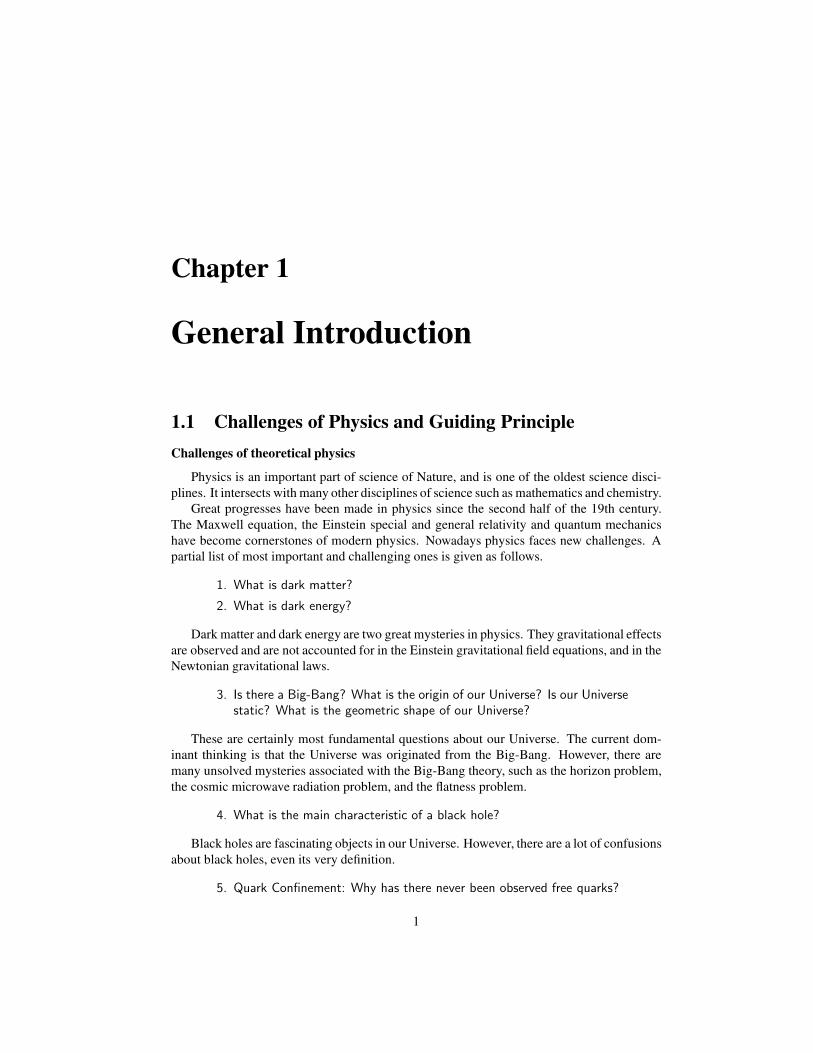
1.1 Challenges of Physics and Guiding Principle
Challenges of theoretical physics
Physics is an important part of science of Nature, and is one of the oldest science disci-
plines. It intersects with many other disciplines of science such as mathematics and chemistry.
Great progresses have been made in physics since the second half of the 19th century.
The Maxwell equation, the Einstein special and general relativity and quantum mechanics
have become cornerstones of modern physics. Nowadays physics faces new challenges. A
partial list of most important and challenging ones is given as follows.
1. What is dark matter?
2. What is dark energy?
Dark matter and dark energy are two great mysteries in physics. They gravitational effects
are observed and are not accounted for in the Einstein gravitational field equations, and in the
Newtonian gravitational laws.
3. Is there a Big-Bang? What is the origin of our Universe? Is our Universestatic? What is the geometric shape of our Universe?
These are certainly most fundamental questions about our Universe. The current dom-
inant thinking is that the Universe was originated from the Big-Bang. However, there are
many unsolved mysteries associated with the Big-Bang theory, such as the horizon problem,
the cosmic microwave radiation problem, and the flatness problem.
4. What is the main characteristic of a black hole?
Black holes are fascinating objects in our Universe. However, there are a lot of confusions
about black holes, even its very definition.
5. Quark Confinement: Why has there never been observed free quarks?
1
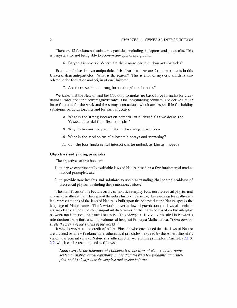
2 CHAPTER 1. GENERAL INTRODUCTION
There are 12 fundamental subatomic particles, including six leptons and six quarks. This
is a mystery for not being able to observe free quarks and gluons.
6. Baryon asymmetry: Where are there more particles than anti-particles?
Each particle has its own antiparticle. It is clear that there are far more particles in this
Universe than anti-particles. What is the reason? This is another mystery, which is also
related to the formation and origin of our Universe.
7. Are there weak and strong interaction/force formulas?
We know that the Newton and the Coulomb formulas are basic force formulas for grav-
itational force and for electromagnetic force. One longstanding problem is to derive similar
force formulas for the weak and the strong interactions, which are responsible for holding
subatomic particles together and for various decays.
8. What is the strong interaction potential of nucleus? Can we derive theYukawa potential from first principles?
9. Why do leptons not participate in the strong interaction?
10. What is the mechanism of subatomic decays and scattering?
11. Can the four fundamental interactions be unified, as Einstein hoped?
Objectives and guiding principles
The objectives of this book are
1) to derive experimentally verifiable laws of Nature based on a few fundamental mathe-
matical principles, and
2) to provide new insights and solutions to some outstanding challenging problems of
theoretical physics, including those mentioned above.
The main focus of this book is on the symbiotic interplay between theoretical physics and
advanced mathematics. Throughout the entire history of science, the searching for mathemat-
ical representations of the laws of Nature is built upon the believe that the Nature speaks the
language of Mathematics. The Newton’s universal law of gravitation and laws of mechan-
ics are clearly among the most important discoveries of the mankind based on the interplay
between mathematics and natural sciences. This viewpoint is vividly revealed in Newton’s
introduction to the third and final volumes of his great Principia Mathematica: “I now demon-
strate the frame of the system of the world.”
It was, however, to the credit of Albert Einstein who envisioned that the laws of Nature
are dictated by a few fundamental mathematical principles. Inspired by the Albert Einstein’s
vision, our general view of Nature is synthesized in two guiding principles, Principles 2.1 &
2.2, which can be recapitulated as follows:
Nature speaks the language of Mathematics: the laws of Nature 1) are repre-
sented by mathematical equations, 2) are dictated by a few fundamental princi-
ples, and 3) always take the simplest and aesthetic forms.
1.2. LAW OF GRAVITY, DARK MATTER AND DARK ENERGY 3
1.2 Law of Gravity, Dark Matter and Dark Energy
Gravity is one of the four fundamental interactions/forces of Nature, and is certainly the first
interaction/force that people studied over centuries, dating back to Aristotle (4th century BC),
to Galileo (late 16th century and early 17th century), to Johannes Kepler (mid 17th century),
to Isaac Newton (late 17th century), and to Albert Einstein (1915).
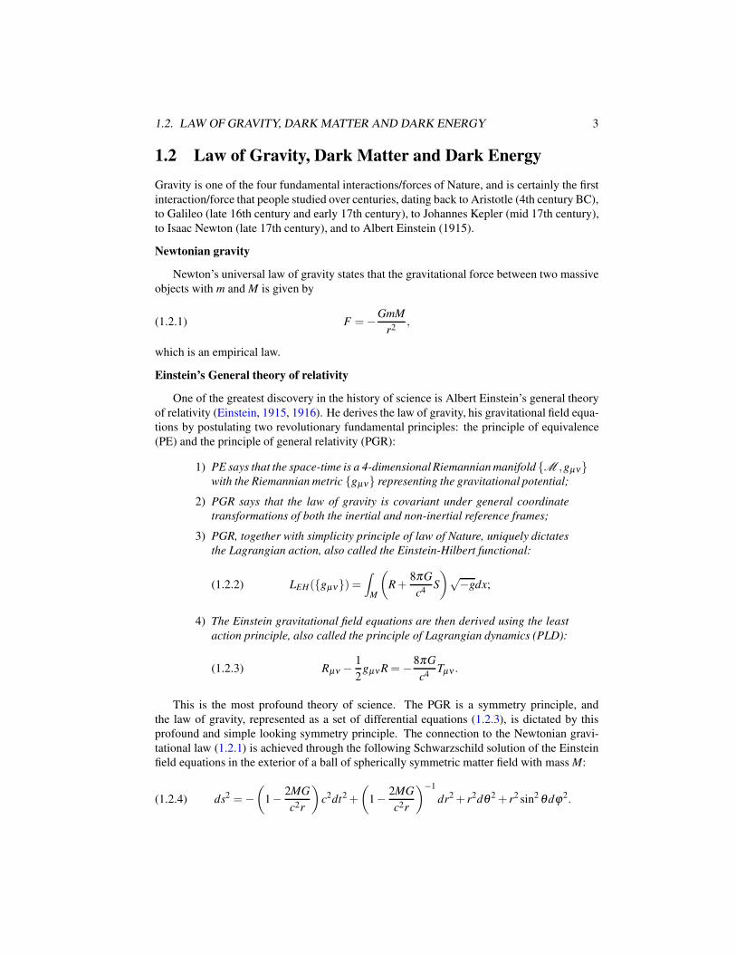
Newtonian gravity
Newton’s universal law of gravity states that the gravitational force between two massive
objects with m and M is given by
(1.2.1) F =−GmM
r2,
which is an empirical law.
Einstein’s General theory of relativity
One of the greatest discovery in the history of science is Albert Einstein’s general theory
of relativity (Einstein, 1915, 1916). He derives the law of gravity, his gravitational field equa-
tions by postulating two revolutionary fundamental principles: the principle of equivalence
(PE) and the principle of general relativity (PGR):
1) PE says that the space-time is a 4-dimensional Riemannian manifold M ,gµνwith the Riemannian metric gµν representing the gravitational potential;
2) PGR says that the law of gravity is covariant under general coordinate
transformations of both the inertial and non-inertial reference frames;
3) PGR, together with simplicity principle of law of Nature, uniquely dictates
the Lagrangian action, also called the Einstein-Hilbert functional:
(1.2.2) LEH(gµν) =∫
M
(R+
8πG
c4S
)√−gdx;
4) The Einstein gravitational field equations are then derived using the least
action principle, also called the principle of Lagrangian dynamics (PLD):
(1.2.3) Rµν −1
2gµνR =−8πG
c4Tµν .
This is the most profound theory of science. The PGR is a symmetry principle, and
the law of gravity, represented as a set of differential equations (1.2.3), is dictated by this
profound and simple looking symmetry principle. The connection to the Newtonian gravi-
tational law (1.2.1) is achieved through the following Schwarzschild solution of the Einstein
field equations in the exterior of a ball of spherically symmetric matter field with mass M:
(1.2.4) ds2 =−(
1− 2MG
c2r
)c2dt2 +
(1− 2MG
c2r
)−1
dr2 + r2dθ 2 + r2 sin2 θdϕ2.
4 CHAPTER 1. GENERAL INTRODUCTION
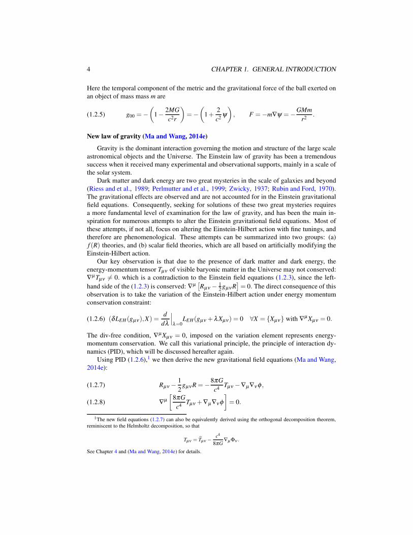
Here the temporal component of the metric and the gravitational force of the ball exerted on
an object of mass mass m are
(1.2.5) g00 =−(
1− 2MG
c2r
)=−
(1+
2
c2ψ
), F =−m∇ψ =−GMm
r2.
New law of gravity (Ma and Wang, 2014e)
Gravity is the dominant interaction governing the motion and structure of the large scale
astronomical objects and the Universe. The Einstein law of gravity has been a tremendous
success when it received many experimental and observational supports, mainly in a scale of
the solar system.
Dark matter and dark energy are two great mysteries in the scale of galaxies and beyond
(Riess and et al., 1989; Perlmutter and et al., 1999; Zwicky, 1937; Rubin and Ford, 1970).
The gravitational effects are observed and are not accounted for in the Einstein gravitational
field equations. Consequently, seeking for solutions of these two great mysteries requires
a more fundamental level of examination for the law of gravity, and has been the main in-
spiration for numerous attempts to alter the Einstein gravitational field equations. Most of
these attempts, if not all, focus on altering the Einstein-Hilbert action with fine tunings, and
therefore are phenomenological. These attempts can be summarized into two groups: (a)
f (R) theories, and (b) scalar field theories, which are all based on artificially modifying the
Einstein-Hilbert action.
Our key observation is that due to the presence of dark matter and dark energy, the
energy-momentum tensor Tµν of visible baryonic matter in the Universe may not conserved:
∇µ Tµν 6= 0. which is a contradiction to the Einstein field equations (1.2.3), since the left-
hand side of the (1.2.3) is conserved: ∇µ[Rµν − 1
2gµνR
]= 0. The direct consequence of this
observation is to take the variation of the Einstein-Hilbert action under energy momentum
conservation constraint:
(1.2.6) (δLEH(gµν),X) =d
dλ
∣∣∣λ=0
LEH(gµν +λ Xµν) = 0 ∀X = Xµν with ∇µ Xµν = 0.
The div-free condition, ∇µXµν = 0, imposed on the variation element represents energy-
momentum conservation. We call this variational principle, the principle of interaction dy-
namics (PID), which will be discussed hereafter again.
Using PID (1.2.6),1 we then derive the new gravitational field equations (Ma and Wang,
2014e):
Rµν −1
2gµνR =−8πG
c4Tµν −∇µ∇ν φ ,(1.2.7)
∇µ
[8πG
c4Tµν +∇µ∇νφ
]= 0.(1.2.8)
1The new field equations (1.2.7) can also be equivalently derived using the orthogonal decomposition theorem,
reminiscent to the Helmholtz decomposition, so that
Tµν = Tµν −c4
8πG∇µ Φν .
See Chapter 4 and (Ma and Wang, 2014e) for details.
1.2. LAW OF GRAVITY, DARK MATTER AND DARK ENERGY 5
In summary, we have derived new law of gravity based solely on first principles, the PE, the
PGR, and the constraint variational principle (1.2.6):
Law of gravity (Ma and Wang, 2014e)
1) (Einstein’s PE). The space-time is a 4D Riemannian manifold M ,gµν,
with the metric gµν being the gravitational potential;
2) The Einstein PGR dictates the Einstein-Hilbert action (1.2.2);
3) The gravitational field equations (1.2.7) and (1.2.8) are derived using PID,
and determine gravitational potential gµν and its dual vector field Φµ =∇µφ ;
4) Gravity can display both attractive and repulsive effect, caused by the dual-
ity between the attracting gravitational field gµν and the repulsive dual
vector field Φµ, together with their nonlinear interactions governed by
the field equations (1.2.7) and (1.2.8).
We remark that it is the duality and both attractive and repulsive behavior of gravity that
maintain the stability of the large scale structure of our Universe.
Modified Newtonian formula from first principles (Ma and Wang, 2014e)
Consider a central matter field with total mass M and with spherical symmetry. We derive
an approximate gravitational force formula:
(1.2.9) F = mMG
[− 1
r2− k0
r+ k1r
], k0 = 4× 10⁻¹⁸km−1, k1 = 10−57km−3.
Here the first term represents the Newton gravitation, the attracting second term stands for
dark matter and the repelling third term is the dark energy. We note that the dark matter
property of the gravity and the approximate gravitational interaction formula are consistent
with the MOND theory proposed by (Milgrom, 1983); see also (Milgrom, 2014) and the
references therein. In particular, our modified new formula is derived from first principles.
Dark matter and dark energy: a property of gravity (Ma and Wang, 2014e)
We have shown that it is the duality between the attracting gravitational field gµν and
the repulsive dual field Φµ = ∇µφ in (1.2.7), and their nonlinear interaction that gives rise
to gravity, and in particular the gravitational effect of dark energy and dark matter.
Also, we show in (Hernandez, Ma and Wang, 2015) that consider the gravitational field
outside of a ball of centrally symmetric matter field. There exist precisely two physical
parameters dictating the two-dimensional stable manifold of asymptotically flat space-time
geometry, such that, as the distance to the center of the ball of the matter field increases,
gravity behaves as Newtonian gravity, then additional attraction due to the curvature of space
(dark matter effect), and repulsive (dark energy effect). This also clearly demonstrates that
both dark matter and dark energy are just a property of gravity.
Of course, one can consider dark matter and dark energy as the energy carried by the
gravitons and the dual gravitons, to addressed in the unified field theory later in this book.
6 CHAPTER 1. GENERAL INTRODUCTION
1.3 First Principles of Four Fundamental Interactions
The four fundamental interactions of Nature are the gravitational interaction, the electromag-
netism, the weak and the strong interactions. Seeking laws of the four fundamental interac-
tions is the most important human endeavor. In this section, we demonstrate that laws for the
four fundamental interactions are determined by the following principles:
1) the principle of general relativity, the principle of gauge invariance, and
the principle of Lorentz invariance, together with the simplicity principle
of laws of Nature, dictates the Lagrangian actions of the four interactions,
and
2) the principle of interaction dynamics and the principle of representation
invariance determines the field equations.
Symmetry principles
We have shown that for gravity, the basic symmetry principle is the Einstein PGR, which
dictates the Einstein-Hilbert action, and induces the gravitational field equations (1.2.7) using
PID.
Quantum mechanics provides a mathematical description about the Nature in the molecule,
the atomic and subatomic levels. Modern theory and experimental evidence have suggested
that the electromagnetic, the weak and the strong interactions obey the gauge symmetry. In
fact, these symmetries and the Lorentz symmetry, together with the simplicity of laws of
Nature dictate the Lagrangian actions for the electromagnetic, the weak and the strong inter-
actions:
Symmetry Dictates Actions of fundamental interactions:
(a) The principle of general relativity dictates the action for gravity, the Einstein-
Hilbert action.
(b) The principle of Lorentz invariance and the principle of gauge invariance,
together with the simplicity principle of laws of Nature, dictate the La-
grangian actions for the electromagnetic, the weak and the strong interac-
tions.
This represents clearly the intrinsic beauty of Nature.
The abelian U(1) gauge theory describes quantum electrodynamics (QED). The non-
abelian SU(N) gauge theory was originated from the early work of (Weyl, 1919; Klein, 1938;
Yang and Mills, 1954). Physically, gauge invariance refers to the conservation of certain
quantum property of the underlying interaction. Such quantum property of the N particles
with wave functions cannot be distinguished for the interaction, and consequently, the energy
contribution of these N particles associated with the interaction is invariant under the general
SU(N) phase (gauge) transformations:
(1.3.1) (Ψ, Gaµτa) =
(ΩΨ, Ga
µΩτaΩ−1 +i
g(∂µ Ω)Ω−1
)∀Ω = eiθ k(x)τk ∈ SU(N).
1.3. FIRST PRINCIPLES OF FOUR FUNDAMENTAL INTERACTIONS 7
Here the N wave functions: Ψ = (ψ1, · · · ,ψN)T represent the N particle fields, the N2 − 1
gauge fields Gaµ represent the interacting potentials between these N particles, and τa | a =
1, · · · ,N2 − 1 is the set of representation generators of SU(N). The gauge symmetry is then
stated as follows:
Principle of Gauge Invariance. The electromagnetic, the weak, and the strong
interactions obey gauge invariance. Namely, the Dirac equations involved in the
three interactions are gauge covariant and the actions of the interaction fields
are gauge invariant under the gauge transformations (1.3.1).
The field equations involving the gauge fields Gaµ are determined by the corresponding
Yang-Mills action, is uniquely determined by both the gauge invariance and the Lorentz in-
variance, together with simplicity of laws of nature:
(1.3.2) LY M
(Ψ,Ga
µ)=
∫
M
[−1
4Gabgµαgνβ Ga
µνGbαβ +Ψ
(iγµ Dµ −
mc
h
)Ψ
]dx,
which is invariant under both the Lorentz and gauge transformations (1.2.3). Here Ψ = Ψ†γ0,
Ψ† = (Ψ∗)T is the transpose conjugate of Ψ, Gab =12tr(τaτ†
b ), λ cab are the structure constants
of τa | a = 1, · · · ,N2 − 1, Dµ is the covariant derivative and Gaµν stands for the curvature
tensor associated with Dµ :
(1.3.3)Dµ = ∂µ + igGk
µτk,
Gaµν = ∂µGa
ν − ∂νGaµ + gλ a
bcGbµGc
ν .
Principle of Interaction Dynamics (PID) (Ma and Wang, 2014e, 2015a)
With the Lagrangian action at our disposal, the physical law of the underlying system
is then represented as the Euler-Lagrangian equations of the action, using the principle of
Lagrangian dynamics (PLD). For example, all laws of classical mechanics can be derived
using PLD. However, in Section 1.1, we have demonstrated that the law of gravity obeys
the principle of interaction dynamics (PID), which takes the variation of the Einstein-Hilbert
action under energy-momentum conservation constraint (1.2.6).
We now state the general form of PID, and then illustrate the validity of PID for all
fundamental interactions.
PID was discovered in (Ma and Wang, 2014e, 2015a), and requires that for the four fun-
damental interactions, the variation be taken under the energy-momentum conservation con-
straints:
PID (Ma and Wang, 2014e, 2015a)
1) For the four fundamental interactions, the Lagrangian actions are given by
(1.3.4) L(g,A,ψ) =
∫
M
L (gµν ,A,ψ)√−gdx,
where g = gµν is the Riemannian metric representing the gravitational
potential, A is a set of vector fields representing the gauge potentials, and
ψ are the wave functions of particles.
8 CHAPTER 1. GENERAL INTRODUCTION
2) The action (1.3.4) satisfy the invariance of general relativity, Lorentz in-
variance, gauge invariance and the gauge representation invariance.
3) The states (g,A,ψ) are the extremum points of (1.3.4) with the divA-free
constraint.
We now illustrate that PID is also valid for both the weak and strong interactions, replac-
ing the classical PLD.
First, PID applied to the Yang-Mills action (1.3.2) takes the following form:
Gab
[∂ νGb
νµ − gλ bcdgαβ Gc
αµGdβ
]− gΨγµτaΨ = (∂µ +αbGb
µ)φa,(1.3.5)
(iγµ Dµ −m)Ψ = 0,(1.3.6)
where the Dirac equations (1.3.6) are the gauge covariant, and are the dynamic equations for
fermions participating the interaction. The right hand side of (1.3.5) is due to PID, with the
operator
∇A = ∂µ +αbGbµ
taken in such a way that αbGbµ is PRI-covariant under the representation transformations
(1.3.8) below.
One important consequence of the PID SU(N) theory is the natural introduction of the
scalar fields φa, reminiscent of the Higgs field in the standard model in particle physics.
Second, for the Yang-Mills action for an SU(N) gauge theory, the resulting Yang-Mills
equations are the Euler-Lagrange equations of the Yang-Mills action:
Gab
[∂ ν Gb
νµ − gλ bcdgαβ Gc
αµGdβ
]− gΨγµτaΨ = 0,(1.3.7)
supplemented with the Dirac equations (1.3.6).
Historically, the most important difficulty encountered by the gauge theory and the field
equations (1.3.7) is that the gauge vectorial field particles Gaµ for the weak interaction are
massless, in disagreement with experimental observations.
A great deal of efforts have been made toward to the modification of the gauge theory by
introducing proper mass generation mechanism. A historically important breakthrough is the
discovery of the mechanism of spontaneous symmetry breaking in subatomic physics. Al-
though the phenomenon was discovered in superconductivity by Ginzburg-Landau in 1951,
the mechanism of spontaneous symmetry breaking in particle physics was first proposed by
Y. Nambu in 1960; see (Nambu, 1960; Nambu and Jona-Lasinio, 1961a,b). The Higgs mech-
anism, introduced in (Higgs, 1964; Englert and Brout, 1964; Guralnik, Hagen and Kibble,
1964), is an ad hoc method based on the Nambu-Jona-Lasinio spontaneous symmetry break-
ing, leading to the mass generation of the vector bosons for the weak interaction.
In all these efforts associated with Higgs fields, the modification of the Yang-Mills action
are artificial as in the case for modifying the Einstein-Hilbert action for gravity.
As we indicated before, the Yang-Mills action is uniquely determined by the gauge sym-
metry, together with the simplicity principle of laws of Nature. All artificial modification of
the action will only lead to certain approximations of the underlying physical laws.
1.3. FIRST PRINCIPLES OF FOUR FUNDAMENTAL INTERACTIONS 9
Third, the PID SU(N) gauge field equations (1.3.5) and (1.3.6) provide a first principle
based mechanism for the mass generation and spontaneous gauge symmetry-breaking: The
αbGbµ on the right-hand side of (1.3.5) breaks the SU(N) gauge symmetry, and the mass
generation follows the Nambu-Jona Lasinio idea.
Fourth, one of the most challenging problems for strong interaction is the quark confinement–
no free quarks have been observed. One hopes to solve this mystery with the quantum chro-
modynamics (QCD) based on the classical SU(3) gauge theory. Unfortunately, as we shall
see later that the classical SU(3) Yang-Mills equations produces only repulsive force, and it
is the dual fields in the PID gauge field equations (1.3.5) that give rise to the needed attraction
for the binding quarks together forming hadrons.
Hence experimental evidence of quark confinement, as well as many other properties
derived from the PID strong interaction model, clearly demonstrates the validity of PID for
strong interactions.
Fifth, from the mathematical point of view, the Einstein field equations are in general non
well-posed, as illustrated by a simple example in Section 4.2.2. In addition, for the classical
Yang-Mills equations, the gauge-fixing problem will also pose issues on the well-posedness
of the Yang-Mills field equations; see Section 4.3.5. The issue is caused by the fact that there
are more equations than the number of unknowns in the system. PID induced model brings
in additional unknowns to the equations, and resolves this problem.
Principle of representation invariance (PRI)
Recently we have observed that there is a freedom to choose the set of generators for
representing elements in SU(N). In other words, basic logic dictates that the SU(N) gauge
theory should be invariant under the following representation transformations of the generator
bases:
(1.3.8) τa = xbaτb,
where X = (xba) are non-degenerate (N2 −1)-th order matrices. Then we can define naturally
SU(N) tensors under the transformations (1.3.8). It is clear then that θ a,Gaµ , and the structure
constants λ cab are all SU(N)-tensors. In addition, Gab = 1
2Tr(τaτ†
b ) is a symmetric positive
definite 2nd-order covariant SU(N)-tensor, which can be regarded as a Riemannian metric on
SU(N). Consequently we have arrived at the following principle of representation invariance,
first discovered by the authors (Ma and Wang, 2014h):
PRI (Ma and Wang, 2014h). For the SU(N) gauge theory, under the represen-
tation transformations (1.3.8),
1) the Yang-Mills action (1.3.2) of the gauge fields is invariant, and
2) the gauge field equations (1.3.5) and (1.3.6) are covariant.
It is clear that PRI is a basic logic requirement for an SU(N) gauge theory, and has
profound physical implications.
First, as indicated in (Ma and Wang, 2014h, 2013a) and in Chapter 4, the field model
based on PID appears to be the only model which obeys PRI. In fact, based on PRI, for the
10 CHAPTER 1. GENERAL INTRODUCTION
gauge interacting fields Aµ and Waµ3
a=1, corresponding to two different gauge groups U(1)for electromagnetism and SU(2) for the weak interaction, the following combination
(1.3.9) αAµ +βW3µ
is prohibited. The reason is that Aµ is an U(1)-tensor with tensor, and W 3µ is simply the
third component of an SU(2)-tensor. The above combination violates PRI. This point of view
clearly shows that the classical electroweak theory violates PRI, so does the standard model.
The difficulty comes from the artificial way of introducing the Higgs field. The PID based
approach for introducing Higgs fields by the authors appears to be the only model obeying
PRI.
Another important consequence of PRI is that for the term αbGbµ in the right-hand side of
the PID gauge field equations (1.3.5), both αb | b= 1, · · · ,N2−1 and Gbµ | b= 1, · · · ,N2−
1 are SU(N) tensors under the representation transformations (1.3.8).
The coefficients αb represent the portions distributed to the gauge potentials by the charge,
represented by the coupling constant g. Then it is clear that
In the field equations (1.3.5) and (1.3.6) of the SU(N) gauge theory for an fun-
damental interaction,
(a) the coupling constant g represents the interaction charge, playing the same
role as the electric charge e in the U(1) abelian gauge theory for quantum
electrodynamics (QED);
(b) the potential
(1.3.10) Gµdef= αbGb
µ
represents the total interacting potential, where the SU(N) covector αb
represents the portions of each interacting potential Gbµ contributed to the
total interacting potential; and
(c) the temporal component G0 and the spatial components ~G = (G1,G2,G3)represent, respectively the interaction potential and interaction magnetic
potential. The force and the magnetic force generated by the interaction
are given by:
F =−g∇G0, Fm =g
c~v× curl ~G,
where ∇ and curl are the spatial gradient and curl operators.
Geometric interaction mechanism
A simple yet the most challenging problem throughout the history of physics is the mech-
anism or nature of a force.
One great vision of Albert Einstein is his principle of equivalence, which, in the mathe-
matical terms, says that the space-time is a 4-dimensional (4D) Riemannian manifold M ,gµν
1.4. SYMMETRY AND SYMMETRY-BREAKING 11
with the metric gµν representing the gravitational potential. In other words, gravity is mani-
fested as the curved effect of the space-time manifold M ,gµν. In essence, gravity is mani-
fested by the gravitational fields gµν ,∇µφ, determined by the gravitational field equations
(1.2.7) and (1.2.8) together with the matter distribution Tµν.
The gauge theory provides a field theory for describing the electromagnetic, the weak and
the strong interactions. The geometry of the SU(N) gauge theory is determined by
1) the complex bundle 2 M ⊗p (C4)N for the wave functions Ψ = (ψ1, · · · ,ψN)
T , repre-
senting the N particles,
2) the gauge interacting fields Gaµ | a = 1, · · · ,N2 − 1, and their dual fields φa | a =
1, · · · ,N2 − 1, and
3) the gauge field equations (1.3.5) coupled with the Dirac equations (1.3.6).
In other words, the geometry of the complex bundle M ⊗p (C4)N , dictated by the gauge
field equations (1.3.5) together with the matter equations (1.3.6), manifests the underlying
interaction.
Consequently, it is natural for us to postulate the Geometric Interaction Mechanism 4.1
for all four fundamental interactions:
Geometric Interaction Mechanism (Ma and Wang, 2014d)
1) (Einstein, 1915) The gravitational force is the curved effect of the time-
space; and
2) the electromagnetic, weak, strong interactions are the twisted effects of the
underlying complex vector bundles M ⊗p Cn.
We note that Yukawa’s viewpoint, entirely different from Einstein’s, is that the other three
fundamental forces—the electromagnetism, the weak and the strong interactions–take place
through exchanging intermediate bosons such as photons for the electromagnetic interaction,
the W± and Z intermediate vector bosons for the weak interaction, and the gluons for the
strong interaction.
It is worth mentioning that the Yukawa Mechanism is oriented toward to computing the
transition probability for particle decays and scattering, and the above Geometric Interaction
Mechanism is oriented toward to establishing fundamental laws, such as interaction poten-
tials, of the four interactions.
1.4 Symmetry and Symmetry-Breaking
As we have discussed so far, symmetry plays a fundamental role in understanding Nature.
In mathematical terms, each symmetry, associated with particular physical laws, consists
2Throughout this book, we use the notation ⊗p to denote ”gluing a vector space to each point of a manifold” to
form a vector bundle. For example,
M ⊗p Cn =
⋃
p∈M
p×Cn
is a vector bundle with base manifold M and fiber complex vector space Cn.
12 CHAPTER 1. GENERAL INTRODUCTION
of three main ingredients: 1) the underlying space, 2) the symmetry group, and 3) tensors,
describing the objects which possess the symmetry.
For example, the Lorentz symmetry is made up of 1) the 4D Minkowski space-time M 4
with the Minkowski metric, 2) the Lorentz group LG, and the Lorentz tensors. For example,
the electromagnetic potential Aµ is a Lorentz tensor, and the Maxwell equations are Lorentz
invariant.
One important point to make is that different physical systems enjoy different symmetry.
For example, gravitational interaction enjoys the symmetry of general relativity, which, amaz-
ingly, dictates the Lagrangian action for the law of gravity. Also, the other three fundamental
interactions obey the gauge and the Lorentz symmetries.
In searching for laws of Nature, one inevitably encounters a system consisting of a number
of subsystems, each of which enjoys its own symmetry principle with its own symmetry
group. To derive the basic law of the system, one approach is to seek for a large symmetry
group, which contains all the symmetry groups of the subsystems. Then one uses the large
symmetry group to derive the ultimate law for the system.
However, often times, the basic logic would dictate that the approach of seeking large
symmetry group is not allowed. For example, as demonstrated earlier, PRI specifically disal-
low the mixing the U(1) and SU(2) gauge interacting potentials in the classical electroweak
theory.
In fact, this demonstrates an inevitably needed departure from the Einstein vision of uni-
fication of the four interactions using large gauge groups.
Our view is that the unification of the four fundamental interactions, as well as the mod-
eling of multi-level physical systems, is achieved through a symmetry-breaking mechanism,
together with PID and PRI. Namely, we postulated in (Ma and Wang, 2014a) and in Sec-
tion 2.1.7 the following Principle of Symmetry-Breaking 2.14:
1) The three sets of symmetries — the general relativistic invariance, the
Lorentz and gauge invariances, and the Galileo invariance — are mutu-
ally independent and dictate in part the physical laws in different levels of
Nature; and
2) for a system coupling different levels of physical laws, part of these sym-
metries must be broken.
Here we mention three examples.
First, for the unification of the four fundamental interaction, the PRI demonstrates that the
unification through seeking large symmetry is not feasible, and the gauge symmetry-breaking
is inevitably needed for the unification. The PID-induced gauge symmetry-breaking, by the
authors (Ma and Wang, 2015a, 2014h,d), offers a symmetry-breaking mechanism based only
on the first principle; see also Chapter 4 for details.
Second, for a multi-particle and multi-level system, its action is dictated by a set of
SU(N1), · · · , SU(Nm) gauge symmetries, and the governing field equations will break some
of these gauge symmetries; see Chapter 6.
Third, in astrophysical fluid dynamics, one difficulty we encounter is that the Newtonian
Second Law for fluid motion and the diffusion law for heat conduction are not compatible
1.5. UNIFIED FIELD THEORY BASED ON PID AND PRI 13
with the principle of general relativity. Also, there are no basic principles and rules for com-
bining relativistic systems and the Galilean systems together to form a consistent system. The
distinction between relativistic and Galilean systems gives rise to an obstacle for establishing
a consistent model of astrophysical dynamics. This difficulty can be circumvented by using
the above mentioned symmetry-breaking principle, where we have to chose the coordinate
system
xµ = (x0,x), x0 = ct and x = (x1,x2,x3),
such that the metric is in the form:
ds2 =−(
1+2
c2ψ(x, t)
)c2dt2 + gi j(x, t)dxidx j.
Here gi j (1 ≤ i, j ≤ 3) are the spatial metric, and ψ represents the gravitational potential.
The resulting system breaks the symmetry of general coordinate transformations, and we call
such symmetry-breaking as relativistic-symmetry breaking.
1.5 Unified Field Theory Based On PID and PRI
One of the greatest problems in physics is to unify all four fundamental interactions. Albert
Einstein was the first person who made serious attempts to this problem.
Most attempts so far have focused on unification through large symmetry, following Ein-
stein’s vision. However, as indicated above, one of the most profound implication of PRI is
that such a unification with a large symmetry group would violate PRI, which is a basic logic
requirement. In fact, the unification should be based on coupling different interactions using
the principle of symmetry-breaking (PSB) instead of seeking for a large symmetry group.
The basic principles for the four fundamental interactions addressed in the previous sec-
tions have demonstrated that the three first principles, PID, PRI and PSB, offer an entirely
different route for the unification, which is one of the main aims of this book:
1) the general relativity and the gauge symmetries dictate the Lagrangian;
2) the coupling of the four interactions is achieved through PID, PRI and
PSB in the unified field equations, which obey the PGR and PRI, but break
spontaneously the gauge symmetry; and
3) the unified field model can be easily decoupled to study individual interac-
tion, when the other interactions are negligible.
Hereafter we address briefly the main ingredients of the unified field theory.
Lagrangian action
Following the simplicity principle of laws of Nature as stated in Principle 2.2, the three ba-
sic symmetries—the Einstein general relativity, the Lorentz invariance and the gauge invariance—
uniquely determine the interaction fields and their Lagrangian actions for the four interac-
tions:
• The Lagrangian action for gravity is the Einstein-Hilbert functional given by (1.2.2);
14 CHAPTER 1. GENERAL INTRODUCTION
• The field describing electromagnetic interaction is the U(1) gauge field Aµ, repre-
senting the electromagnetic potential, and the Lagrangian action density is
(1.5.1) LEM =−1
4AµνAµν +ψe(iγµDµ −me)ψ
e,
in which the first term stands for the scalar curvature of the vector bundle M ⊗p C4.
The covariant derivative and the field strength are given by
Dµψe = (∂µ + ieAµ)ψe, Aµν = ∂µAν − ∂νAµ .
• For the weak interaction, the SU(2) gauge fields W aµ |a = 1,2,3 are the interacting
fields, and the SU(2) Lagrangian action density LW for the weak interaction is the
standard Yang-Mills action density as given by (1.3.2).
• The SU(3) gauge action density LS for the strong interaction is also in the standard
Yang-Mills form given by (1.3.2), and the strong interaction fields are the SU(3) gauge
fields Skµ | 1 ≤ k ≤ 8, representing the 8 gluon fields.
It is clear that the action coupling the four fundamental interactions is the natural combi-
nation of the Einstein-Hilbert functional, the standard U(1),SU(2),SU(3) gauge actions for
the electromagnetic, weak and strong interactions:
(1.5.2) L(gµν,Aµ ,W a
µ,Skµ)=∫
M
[LEH +LEM +LW +LS]√−gdx,
which obeys all the symmetric principles, including principle of general relativity, the Lorentz
invariance, the U(1)× SU(2)× SU(3) gauge invariance and PRI.
PID unified field equations
With PID, the PRI covariant unified field equations are then given by:
Rµν −1
2gµνR+
8πG
c4Tµν =
[∇µ +α0Aµ +α1
bW bµ +α2
k Skµ
]φG
ν ,(1.5.3)
∂ µ(∂µAν − ∂νAµ)− eJν =[∇ν +β 0Aν +β 1
bW bν +β 2
k Skν
]φ e,(1.5.4)
Gwab
[∂ µW b
µν − gwλ bcdgαβW c
ανW dβ
]− gwJνa(1.5.5)
=
[∇ν + γ0Aν + γ1
bW bν + γ2
k Skν −
1
4m2
wxν
]φw
a ,
Gsk j
[∂ µ S
jµν − gsΛ
jcdgαβ Sc
ανSdβ
]− gsQνk(1.5.6)
=
[∇ν + δ 0Aν + δ 1
b W bν + δ 2
k Skν −
1
4m2
s xν
]φ s
k ,
(iγµ Dµ −m)Ψ = 0,(1.5.7)
where Ψ= (ψe,ψw,ψs)T stands for the wave functions for all fermions, participating respec-
tively the electromagnetic, the weak and the strong interactions, and the current densities are
defined by
Jν = ψeγν ψe, Jνa = ψwγν σaψw, Qνk = ψsγν τkψs.(1.5.8)
1.5. UNIFIED FIELD THEORY BASED ON PID AND PRI 15
Equations (1.5.7) are the gauge covariant Dirac equations for all fermions participating
the four fundamental interactions. The left-hand sides of the field equations (1.5.3)-(1.5.6) are
the same as the classical Einstein equations and the standard U(1)× SU(2)× SU(3) gauge
field equations. The right-hand sides of are due to PID, and couple the four fundamental
interactions.
Duality
In the field equations (1.5.3)-(1.5.6), there exists a natural duality between the interaction
fields (gµν ,Aµ ,Waµ ,S
kµ) and their corresponding dual fields (φG
µ ,φ e,φwa ,φ
sk ). This duality
can be viewed as the duality between mediators and the duality between interacting forces,
summarized as follows:
(a) Duality of mediators. Each interaction mediator possesses a dual field
particle, called the dual mediator, and if the mediator has spin-k, then its
dual mediator has spin-(k− 1).
(b) Duality of interacting forces. Each interaction generates both attracting
and repelling forces. Moreover, for each pair of dual fields, the even-spin
field generates an attracting force, and the odd-spin field generates a re-
pelling force.
A few remarks are now in order.
First, from the (phenomenological) weakton theory of elementary particles to be intro-
duced later, that each mediator and its corresponding dual mediator are the same type of
particles with the same constituents, but with different spins.
Second, from the duality of the mediators induced from the first principle PID, we con-
jecture that in addition to the neutral Higgs found by LHC in 2012, there must be two charged
massive spin−0 Higgs particles.
Third, the duality of interacting forces demonstrates that all four forces can be both attrac-
tive and repulsive. For example, as the distance of two massive objects increases, the gravita-
tional force displays attraction as the Newtonian gravity, more attraction than the Newtonian
gravity in the galaxy scale, and repulsion in a much larger scale.
Fourth, as we shall see later, the 8 gluon fields produces repulsive force, and it is their
dual fields that produce the needed attraction for quark confinement. This gives a strong
observational evidence for the existence of the dual gluons and for the valid and necessity of
PID.
Decoupling
The unified field model can be easily decoupled to study each individual interaction when
other interactions are negligible. In other words, PID is certainly applicable to each individual
interaction. For gravity, for example, PID offers to a new gravitational field model, leading
to a unified model for dark energy and dark matter as described earlier in this introduction.

16 CHAPTER 1. GENERAL INTRODUCTION
1.6 Theory of Strong Interactions
The strong interaction is responsible for the nuclear force that binds protons and neutrons
(nucleons) together to form the nucleus of an atom, and is the force that holds quarks together
to form protons, neutrons, and other hadron particles. The current theory of strong interaction
is the quantum chromodynamics (QCD), based on an SU(3) non-Abelian gauge theory.
Two most important observed basic properties of the strong interaction are the asymptotic
freedom and the quark confinement. The theoretical understanding of these properties are still
lacking. There have been many attempts such as the lattice QCD, which is developed in part
for the purpose of understanding the quark confinement.
Modern theory of QCD leaves a number of key problems open for a long time, including
1) (Quark confinement) Why is there no observed quark?
2) Why is there asymptotic freedom?
3) What is the strong interaction potential?
4) Can one derive the Yukawa potential from first principles?
5) Why is the strong force short-ranged?
These are longstanding problems, and the new field theory for strong interaction based on
PID and PRI completely solves these open problems. We now present some basic ingredients
of this new development, and we refer the interested readers to (Ma and Wang, 2014c) and
Section 4.5 for details.
PID SU(3) gauge field equations
The strong interaction field equations decoupled from the unified field model are
Gsk j
[∂ µS
jµν − gsΛ
j
cdgαβ ScανSd
β
]− gsQνk =
[∂ν + δ 2
k Skν −
1
4m2
s xν
]φ s
k ,(1.6.1)
[iγµ(
∂µ + igsSkµτk
)−mq
]ψ = 0.(1.6.2)
1. Gluons and dual scalar gluons. For the strong interaction, the field equations induce
a duality between the eight spin-1 massless gluons, described by the SU(3) gauge fields
Skµ | k = 1, · · · ,8, and the eight spin-0 dual gluons, described by the dual fields φ s
k | a =1, · · · ,8. As we shall see from the explianation of quark confinements gluons and their dual
gluons are confined in hadrons.
2. Attracting and repulsive behavior of strong force. As indicated before and from the
strong interaction potentials derived hereafter, strong interaction can display both attracting
and repulsive behavior. The repulsive behavior is due mainly to the spin-1 gluon fields, and
the attraction is caused by the spin-0 dual gluon fields.
Layered strong interaction potentials
Different from gravity and electromagnetic force, strong interaction is of short-ranged
with different strengths in different levels. For example, in the quark level, strong interaction
1.6. THEORY OF STRONG INTERACTIONS 17
confines quarks inside hadrons, in the nucleon level, strong interaction bounds nucleons in-
side atoms, and in the atom and molecule level, strong interaction almost diminishes. This
layered phenomena can be well-explained using the unified field theory based on PID and
PRI.
One key ingredient is total interaction as the consequence of PRI addressed above. For
the strong interaction, in view of (1.3.10), the total strong interaction potential is defined by
δ 2k Sk
ν on the right hand side of (1.6.1):
(1.6.3) Sµdef= δ 2
k Skµ = (S0,S1,S2,S3), Φ
def= S0.
The temporal component S0, denoted by Φ, gives rise to the strong force between two ele-
mentary particles carrying strong charges:
(1.6.4) F =−gs∇Φ.
From the field equations (1.6.1) and (1.6.2), we derive in Section 4.5.2 that for a particle
with N strong charges and radius ρ , its strong interaction potential are given by (4.5.39) and
recast here convenience:
(1.6.5)
Φ = gs(ρ)
[1
r− A
ρ(1+ kr)e−kr
],
gs(ρ) = N
(ρw
ρ
)3
gs,
where gs is the strong charge of w∗-weakton, the ρw is the radius of the w∗-weakton, A is a
dimensionless constant depending on the particle, and 1/k is the radius of strong attraction
of particles. Phenomenologically, we can take
(1.6.6)1
k=
10−18 cm for w∗− weaktons,
10−16 cm for quarks,
10−13 cm for neutreons,
10−7 cm for atom/molecule,
and the resulting layered formulas of strong interaction potentials are called the w∗-weakton
potential Φ0, the quark potential Φq, the nucleon/hadron potential Φn and the atom/molecule
potential Φa.
Quark confinement
Quark confinement is a challenging problem in physics. Quark model was confirmed by
many experiments. However, no any single quark is found ever. This fact suggests that the
quarks were permanently bound inside a hadron, which is called the quark confinement. Up
to now, no other theories can successfully describe the quark confinement phenomena. The
direct reason is that all current theories for interactions fail to provide a successful strong
interaction potential to explain the various level strong interactions.
18 CHAPTER 1. GENERAL INTRODUCTION
With the strong interaction potential (1.6.5), we can calculate the strong interaction bound
energy E for two same type of particles:
(1.6.7) E = g2s (ρ)
[1
r− A
ρ(1+ kr)e−kr
].
The quark confinement can be well explained from the viewpoint of the strong quark
bound energy Eq and the nucleon bound energy En. In fact, by (1.6.7) we can show that
(1.6.8) Eq = 1020En ∼ 1018GeV.
This clearly shows that the quarks is confined in hadrons, and no free quarks can be found.
Asymptotic freedom and short-range nature of the strong interaction
Asymptotic freedom was discovered and described by (Gross and Wilczek, 1973; Politzer,
1973). Using the strong interaction potential (1.6.5), we can clearly demonstrate the asymp-
totic freedom property and the short-ranged nature of the strong interaction.
1.7 Theory of Weak Interactions
The new weak interaction theory based on PID and PRI was first discovered by (Ma and Wang,
2013a). As addressed earlier, the weak interaction obeys the SU(2) gauge symmetry, which
dictates the standard SU(2) Yang-Mills action. By PID and PRI, the field equations of the
weak interaction are given by:
Gwab
[∂ µW b
µν − gwλ bcdgαβW c
ανW dβ
]− gwψwγν σaψw =
[∂µ + γ1
bW bµ − 1
4m2
wxµ
]φw
a ,(1.7.1)
(iγµ Dµ −ml)ψw = 0.(1.7.2)
1. Higgs fields from first principles. The right-hand side of (1.7.1) is due to PID, leading
naturally to the introduction of three scalar dual fields. The left-hand side of (1.7.1) represents
the intermediate vector bosons W± and Z, and the dual fields represent two charged Higgs
H± (to be discovered) and the neutral Higgs H0, with the later being discovered by LHC in
2012.
It is worth mentioning that the right-hand side of (1.7.1), involving the Higgs fields, can
not be generated by directly adding certain terms in the Lagrangian action, as in the case for
the new gravitational field equations derived in (Ma and Wang, 2014e).
2. Duality. We establish a natural duality between weak gauge fields Waµ, representing
the W± and Z intermediate vector bosons, and three bosonic scalar fields φwa , representing
both two charged and one neutral Higgs particles H±, H0.
3. Spontaneous gauge symmetry-breaking. PID induces naturally spontaneous symmetry
breaking mechanism. By construction, it is clear that the Lagrangian action LW obeys the
SU(2) gauge symmetry, the PRI and the Lorentz invariance. Both the Lorentz invariance
and PRI are universal principles, and, consequently, the field equations (1.7.1) and (1.7.2)
1.8. NEW THEORY OF BLACK HOLES 19
are covariant under these symmetries. The gauge symmetry is spontaneously breaking in the
field equations (1.7.1), due to the presence of the terms in the right-hand side, derived by PID.
This term generates the mass for the vector bosons.
4. Weak charge and weak potential. By PRI, the SU(2) gauge coupling constant gw plays
the role of weak charge, responsible for the weak interaction.
Also, PRI induces an important SU(2) constant vector γ1b. The components of this
vector represent the portions distributed to the gauge potentials W aµ by the weak charge gw.
Hence the (total) weak interaction potential is given by the following PRI representation
invariant
(1.7.3) Wµ = γ1aW a
µ = (W0,W1,W2,W3),
and the weak charge potential and weak force are as
(1.7.4)Φw =W0 the time component of Wµ ,
Fw =−gw(ρ)∇Φw,
where gw(ρ) is the weak charge of a particle with radius ρ .
5. Layered formulas for the weak interaction potential. The weak interaction is also
layered, and we derive from the field equations the following
(1.7.5)
Φw = gw(ρ)e−kr
[1
r− B
ρ(1+ 2kr)e−kr
],
gw(ρ) = N
(ρw
ρ
)3
gw,
where Φw is the weak force potential of a particle with radius ρ and carrying N weak charges
gw, taken as the unit of weak charge gs for each weakton (Ma and Wang, 2015b), ρw is the
weakton radius, B is a parameter depending on the particles, and 1/k = 10−16 cm represents
the force-range of weak interactions.
6. The layered weak interaction potential formula (1.7.5) shows clearly that the weak in-
teraction is short-ranged. Also, it is clear that the weak interaction is repulsive, asymptotically
free, and attractive when the distance of two particles increases.
1.8 New Theory of Black Holes
The concept of black holes is essentially developed following the Karl Schwarzschild’s deriva-
tion of the Schwarzschild solution for the Einstein gravitational field equations. In the exterior
of spherically symmetric ball of mass, the solution is given by
(1.8.1) ds2 =−(
1− Rs
r
)c2dt2 +
(1− Rs
r
)−1
dr2 + r2dθ 2 + r2 sin2 θdϕ2,
where
(1.8.2) Rs =2MG
c2
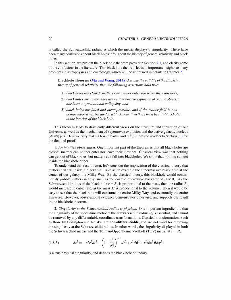
20 CHAPTER 1. GENERAL INTRODUCTION
is called the Schwarzschild radius, at which the metric displays a singularity. There have
been many confusions about black holes throughout the history of general relativity and black
holes.
In this section, we present the black hole theorem proved in Section 7.3, and clarify some
of the confusions in the literature. This black hole theorem leads to important insights to many
problems in astrophysics and cosmology, which will be addressed in details in Chapter 7.
Blackhole Theorem (Ma and Wang, 2014a) Assume the validity of the Einstein
theory of general relativity, then the following assertions hold true:
1) black holes are closed: matters can neither enter nor leave their interiors,
2) black holes are innate: they are neither born to explosion of cosmic objects,
nor born to gravitational collapsing, and
3) black holes are filled and incompressible, and if the matter field is non-
homogeneously distributed in a black hole, then there must be sub-blackholes
in the interior of the black hole.
This theorem leads to drastically different views on the structure and formation of our
Universe, as well as the mechanism of supernovae explosion and the active galactic nucleus
(AGN) jets. Here we only make a few remarks, and refer interested readers to Section 7.3 for
the detailed proof.
1. An intuitive observation. One important part of the theorem is that all black holes are
closed: matters can neither enter nor leave their interiors. Classical view was that nothing
can get out of blackholes, but matters can fall into blackholes. We show that nothing can get
inside the blackhole either.
To understand this result better, let’s consider the implication of the classical theory that
matters can fall inside a blackhole. Take as an example the supermassive black hole at the
center of our galaxy, the Milky Way. By the classical theory, this blackhole would contin-
uously gobble matters nearby, such as the cosmic microwave background (CMB). As the
Schwarzschild radius of the black hole r = Rs is proportional to the mass, then the radius Rs
would increase in cubic rate, as the mass M is proportional to the volume. Then it would be
easy to see that the black hole will consume the entire Milky Way, and eventually the entire
Universe. However, observational evidence demonstrates otherwise, and supports our result
in the blackhole theorem.
2. Singularity at the Schwarzschild radius is physical. One important ingredient is that
the singularity of the space-time metric at the Schwarzschild radius Rs is essential, and cannot
be removed by any differentiable coordinate transformations. Classical transformations such
as those by Eddington and Kruskal are non-differentiable, and are not valid for removing
the singularity at the Schwarzschild radius. In other words, the singularity displayed in both
the Schwarzschild metric and the Tolman-Oppenheimer-Volkoff (TOV) metric at r = Rs
(1.8.3) ds2 =−euc2dt2 +
(1− r2
R2s
)−1
dr2 + r2dθ 2 + r2 sin2 θdϕ2,
is a true physical singularity, and defines the black hole boundary.
1.9. THE UNIVERSE 21
3. Geometric realization of a black hole. As described in Section 4.1 in (Ma and Wang,
2014a) and in Section 7.3.1, the geometrical realization of a black hole, dictated by the
Schwarzschild and TOV metrics, clearly manifests that the real world in the black hole is
a hemisphere with radius Rs embedded in R4, and at the singularity r = Rs, the tangent space
of the black hole is perpendicular to the coordinate space R3.
This geometric realization clearly demonstrates that the disk in the realization space R3
is equivalent to the real world in the black hole. If the outside observer observes that nothing
gets inside the black hole, then nothing will get inside the black hole in the reality as well.
1.9 The Universe
Geometry and origin of our Universe
Modern cosmology adopts the view that our Universe is formed through the Big-Bang
or Big-Bounce; see among others (Harrison, 2000; Kutner, 2003; Popławski, 2012; Roos,
2003). Based on our new insights on black holes, we have reached very different conclusions
on the structure and formation of our Universe.
It is clear that the large scale structure of our Universe is essentially dictated by the law
of gravity, which is based on Einstein’s two principles: the principle of general relativity
and the principle of equivalence, as addressed in Section 1.1. Also, strong cosmological
observational evidence suggests that the large scale Universe obey the cosmological principle
that the Universe is homogeneous and isotropic.
Basic assumptions
(a) the Einstein theory of general relativity, and
(b) the cosmological principle.
With Assumption (a) above, we have our blackhole theorem, Theorem 7.15, at our dis-
posal. Then we can draw a number of important conclusions on the structure of our Universe.
1. Let E and M be the total energy and mass of the Universe:
(1.9.1) E = kinetic+ electromagnetic+ thermal+Ψ, M = E/c2,
where Ψ is the energy of all interaction fields. The total mass M dictates the Schwarzschild
radius Rs.
If our Universe were born to the Big-Bang, assuming at the initial stage, all energy is
concentrated in a ball with radius R0 < Rs, by the theory of black holes, then the energy
contained in BR0must generate a black hole in R3 with fixed radius Rs as defined by (1.8.2).
If we assume that at certain stage, the Universe were contained in ball of a radius R with
R0 < R < Rs, then we can prove that the Universe must contain a sub-black hole with radius
r given by
r =
√R
Rs
R.
Based on this property, the expansion of the Universe, with increasing R to Rs, will give rise to
an infinite sequence of black holes with one embedded to another. Apparently, this scenario
22 CHAPTER 1. GENERAL INTRODUCTION
is clearly against the observations of our Universe, and demonstrates that our Universe cannot
be originated from a Big-Bang.
2. By the cosmological principle, given the energy density ρ0 > 0 of the Universe, based
on the Schwarzschild radius, the Universe will always be bounded in black hole, which is an
open ball of radius:
Rs =
√3c2
8πGρ0
.
This immediately shows that there is no unbounded universe. Consequently, since a black
hole is unable to expand and shrink, we arrive immediately from the above analysis that our
Universe must be static, and not expanding.
Notice that the isotropy requirement in the cosmological principle excludes the globular
open universe scenario. Consequently, we have shown that our Universe must be a closed 3D
sphere S3.
In summary, we have proved two theorems, Theorems 7.27-7.28, on the geometry and
structure of our Universe, which have been discovered and proved in (Ma and Wang, 2014a,
Theorems 6.2 & 6.3):
Theorem on Structure of our Universe. Assume the Einstein theory of gen-
eral relativity, and the principle of cosmological principle, then the following
assertions hold true:
1) our Universe is not originated from a Big-Bang, and is static;
2) the topological structure of our Universe is the 3D sphere S3 such that to
each observer, the corresponding equator with the observer at the center
of the hemisphere can be viewed as the black hole horizon;
3) the total mass Mtotal in the Universe includes both the cosmic observable
mass M and the non-observable mass, regarded as dark matter, due to the
space curvature energy; and
4) a negative pressure is present in our Universe to balance the gravitational
attracting force, and is due to the gravitational repelling force, also called
dark energy.
It is clear that this theorem changes drastically our view on the geometry and the origin
of the Universe. Inevitably, a number of important questions need to be addressed for this
scenario of our Universe. Hereafter we examine a few most important problems.
Redshift problem
The natural and important question that one has to answer is the consistency with as-
tronomical observations, including the cosmic edge, the flatness, the horizon, the redshift,
and the cosmic microwave background (CMB) problems. These problems can now be eas-
ily understood based on the structure of the Universe and the blackhole theorem we derived.
Hereafter we focus only on the redshift and the CMB problems.
The most fundamental problem is the redshift problem. Observations clearly show that
light coming from a remote galaxy is redshifted, and the farther away the galaxy is, the larger
1.9. THE UNIVERSE 23
the redshift. In modern astronomy and cosmology, it is customary to characterize the redshift
by a dimensionless quantity z in the formula
(1.9.2) 1+ z =λobserv
λemit
,
where λobserv and λemit represent the observed and emitting wavelenths.
There are three sources of redshifts: the Doppler effect, the cosmological redshift, and the
gravitational redshift. If the Universe is not considered as a black hole, then the gravitational
redshift and the cosmological redshift are both too small to be significant. Hence, modern
astronomers have to think that the large port of the redshift is due to the Doppler effect.
However, due to black hole properties of our Universe, the black hole and cosmological
redshifts cannot be ignored. Due to the horizon of the sphere, for an arbitrary point in the
spherical Universe, its opposite hemisphere relative to the point is regarded as a black hole.
Hence, g00 can be approximatively taken as the Schwarzschild solution for distant objects as
follows
−g00(r) = α(r)
(1− Rs
r
), α(0) = 2, α(Rs) = 1, α ′(r)< 0,
where r = 2Rs − r for 0 ≤ r < Rs is the distance from the light source to the opposite radial
point, and r is the distance from the light source to the point. Then we derive the following
redshift formula, which is consistent with the observed redshifts:
(1.9.3) 1+ z =1√
α(r)(1− Rsr)=
√2Rs − r√
α(r)(Rs − r)for 0 < r < Rs.
CMB problem
In 1965, two physicists A. Penzias and R. Wilson discovered the low-temperature cosmic
microwave background (CMB) radiation, which fills the Universe, and it has been regarded
as the smoking gun for the Big-Bang theory. However, based on the unique scenario of our
Universe we derived, it is the most natural thing that there exists a CMB, because the Uni-
verse has always been there as a black-body, and CMB is a result of blackbody equilibrium
radiation.
Dark matter and dark energy
Conclusion 4) in the above results for our Universe shows that the observable cosmic mass
M, and the total mass Mtotal which includes both M and the non-observable mass caused by
space curvature energy, enjoy the following relation:
(1.9.4) Mtotal = 3πM/2
The difference Mtotal−M can be regarded as the dark matter. Astronomical observations have
shown that the measurable mass M is about one fifth of total mass Mtotal.
Also, the static Universe has to possess a negative pressure to balance the gravitational
attracting force. The negative pressure is actually the effect of the gravitational repelling
force, attributed to dark energy.
24 CHAPTER 1. GENERAL INTRODUCTION
Equivalently, the above interpretation of dark matter and dark energy is consistent with
the theory based on the new PID gravitational field equations discovered by (Ma and Wang,
2014e) and addressed in detail in Chapter 4. It is clear now that gravity can display both
attractive and repulsive effect, caused by the duality between the attracting gravitational field
gµν and the repulsive dual vector field Φµ, together with their nonlinear interactions
governed by the field equations. Consequently, dark energy and dark matter phenomena are
simply a property of gravity. The detailed account of this relation is addressed in Section 7.6,
based in part on (Hernandez, Ma and Wang, 2015).
PID-cosmological model
One of the main motivations for the introduction of the Big-Bang theory and for the ex-
panding universe is that the Friedamann solution of the Einstein gravitational field equations
demonstrated that the Einstein theory must produce a variable size universe; see Conclusions
of Friedmann Cosmology 7.23. Also, it is classical that bringing the cosmological constant
Λ into the Einstein field equations will lead to an unstable static universe.
We have demonstrated that the right cosmological model should be derived from the new
gravitational field equations (1.2.7), taking into consideration the presence of dark matter and
dark energy. In this case, based on the cosmological principle, the the metric of a homoge-
neous spherical universe is of the form
(1.9.5) ds2 =−c2dt2 +R2
[dr2
1− r2+ r2(dθ 2 + sin2 θdϕ2)
],
where R = R(t) is the cosmic radius. We deduce then from (1.2.7) the following PID-
cosmological model, with ϕ = φ ′′:
(1.9.6)
R′′ =−4πG
3
(ρ +
3p
c2+
ϕ
8πG
)R,
(R′)2 =1
3(8πGρ +ϕ)R2 − c2,
ϕ ′+3R′
Rϕ =−24πG
c2
R′
Rp,
supplemented with the equation of state:
(1.9.7) p = f (ρ ,ϕ).
Note that only two equations in (1.9.6) are independent.
Also, the model describing the static Universe is the equation of state (1.9.7) together
with the stationary equations of (1.9.6), which are equivalent to the form
(1.9.8)
ϕ =−8πG
(ρ +
3p
c2
),
p =− c4
8πGR2.
1.10. SUPERNOVAE EXPLOSION AND AGN JETS 25
1.10 Supernovae Explosion and AGN Jets
Supernovae explosion and the active galactic nucleus (AGN) jets are among the most impor-
tant astronomical phenomena, which are lack of reasonable explanation.
Relativistic, magnetic and thermal effects are main ingredients in astrophysical fluid dy-
namics, and are responsible for many astronomical phenomena. The thermal effect is de-
scribed by the Rayleigh number Re:
(1.10.1) Re =mGr0r1β
κν
T0 −T1
r1 − r0
,
where T0 and T1 are the temperatures at the bottom and top of an annular shell region r0 <r < r1; see e.g. (7.1.74) for other notations used here.
Based on our theory of black holes, including in particular the incompressibility and
closedness of black holes, the relativistic effect is described by the δ -factor:
(1.10.2) δ =2mG
c2r0
.
where m is the mass of the core 0 < r < r0.
Consider e.g. an active galactic nucleus (AGN), which occupies a spherical annular shell
region Rs < r < R1, where Rs is the Schwarzschild radius of the black hole core of the galaxy.
Then r0 = Rs and the δ -factor is δ = 1. The relativistic effect is then reflected in the radial
force
Fr =ν
2α
∂
∂ r
(1
α
dα
drPr
), α =
(1− Rs
r
)−1
,
which gives rise to a huge explosive force near r = Rs:
(1.10.3)ν
1−Rs/r
R2s
r4Pr.
The relativistic effect is also reflected in the electromagnetic energy:
ν0
2α
∂
∂ r
(1
α
dα
drHr
),
which consists of a huge explosive electromagnetic energy near r = Rs:
(1.10.4)ν0
1−Rs/r
R2s
r4Hr.
The basic mechanism of the formation of AGN jets is that the radial temperature gradient
causes vertical Benard convection cells. Each Benard convection cell has a vertical exit,
where the circulating gas is pushed by the radial force, and then erupts leading to a jet.
Each Benard convection cell is also an entrance, where the external gas is attracted into the
nucleus, is cycloaccelerated by the radial force as well, goes down to the interior boundary
r = Rs, and then is pushed toward to the exit. Thus the circulation cells form jets in their exits
and accretions in their entrances.
26 CHAPTER 1. GENERAL INTRODUCTION
This mechanism can also be applied to supernovae explosion. When a very massive red
giant completely consumes its central supply of nuclear fuels, its core collapses. Its radius r0
begins to decrease, and consequently the δ -factor increases. The huge mass m and the rapidly
reduced radius r0 make the δ -factor approaching one. The thermal convection gives rise to
an outward radial circulation momentum flux Pr. Then the radial force as in (1.10.3) will lead
to the supernova explosion. Also, Pr = 0 at r = r0, where r0 is the radius of blackhole core of
supernovae. Consequently, the supernova’s huge explosion preserves a smaller ball, yielding
a neutron star.
1.11 Multi-Particle Systems and Unification
The field theory for multi-particle system was discovered by (Ma and Wang, 2014d). Clas-
sical quantum dynamic equations describe single particle systems. The existing model for a
multi-particle system is non-relativistic and is based on prescribing the interaction between
particles using such potentials as the Coulomb potential.
As far as we know, there is still no good model for a multi-particle system, which takes
also into consideration the dynamic interactions between particles. The main obstacle for es-
tablishing a field theory for an interacting multi-particle system is the lack of basic principles
to describe the dynamic interactions of the particles.
Basic postulates for interacting multi-particle systems
To seek the needed principles, we proceed with three observations.
1. One natural outcome of the field theory of four interactions developed recently by
the authors and addressed in the previous sections is that the coupling constants for the
U(1)× SU(2)× SU(3) gauge theory play the role of the three charges e, gw and gs for elec-
tromagnetism, the weak and the strong interaction. These charges generate interacting fields
among the interacting particles.
Now we consider an N-particle system with each particle carrying an interaction charge
g. Let this be a fermionic system, and the Dirac spinors be given by
Ψ = (ψ1, · · · ,ψN)T ,
which obeys the Dirac equations:
(1.11.1) iγµDµΨ+MΨ = 0,
where M is the mass matrix, and
(1.11.2) DµΨ = ∂µ Ψ+ igGΨ,
where G = (Gi jµ ) is an Hermitian matrix, representing the interacting potentials between the
N-particles generated by the interaction charge g.
Now let
τ0, τ1, · · · , τK | K = N2 − 1
1.11. MULTI-PARTICLE SYSTEMS AND UNIFICATION 27
be a basis of the set of all Hermitian matrices, where τ0 = I is the identity, and τa (1 ≤ a ≤N2 − 1) are the traceless Hermitian matrices. Then the Hermitian matrix G = (G
i jµ ) and the
differential operator Dµ in (1.11.1) can be expressed as
G = G0µ I+Ga
µτa,
Dµ = ∂µ + igG0µ + igGa
µτa.
Consequently the Dirac equations (1.11.1) are rewritten as
(1.11.3) iγµ [∂µ + igG0µ + igGa
µτa]Ψ+MΨ = 0.
2. The energy contributions of the N particles are indistinguishable, which implies the
SU(N) gauge invariance. Hence (1.11.3) are exactly the Dirac equations in the form of SU(N)gauge fields Ga
µ | 1 ≤ a ≤ N2 − 1 with a given external interaction field G0µ .
3. The SU(N) gauge theory of N particles must obey PRI. Consequently there exists a
constant SU(N) tensor
αNa = (αN
1 , · · · ,αNN ),
such that the contraction field using PRI
(1.11.4) Gµ = αNa Ga
is independent of the SU(N) representation τa, and is the interaction field which can be ex-
perimentally observed.
With these three observations, it is natural for us to introduce the following postulate,
which is also presented as Postulates 6.25–6.27 in Chapter 6:
Postulates for interacting multi-particle systems
1) the Lagrangian action for an N-particle system satisfy the SU(N) gauge
invariance;
2) gGaµ represent the interaction potentials between the particles; and
3) for an N-particle system, only the interaction field Gµ in (1.11.4) can be
measured, and is the interaction field under which this system interacts with
other external systems.
Field Equations for Multi-Particle System
Multi-particle systems are layered, and with the above postulates and basic symmetry
principles, we are able to determine in a unique fashion field equations for different multi-
particle systems.
For example, given an N-particle system consisting of N fermions with given charge g, the
SU(N) gauge symmetry dictates uniquely the Lagrangian density, given in two parts: 1) the
sector of SU(N) gauge fields LG, and 2) the Dirac sector of particle fields LD , as described
earlier in the SU(N) gauge theory. The combined action is 1) SU(N) gauge invariant, 2)
28 CHAPTER 1. GENERAL INTRODUCTION
representation invariant (PRI), and 3) Lorentz invariant. The field equations are then derived
by using PID:
Gab
[∂ ν Gb
νµ − gλ bcdgαβ Gc
αµGdβ
]− gΨγµτaΨ =
[∂µ − k2
4xµ + gGµ + gG0
µ
]φa,(1.11.5)
iγµ[∂µ + igG0
µ + igGaµ τa
]Ψ−MΨ = 0,(1.11.6)
for 1 ≤ a ≤ N2 −1, where G0µ is the interaction field of external systems, and Gµ = αaGa
µ . It
is important to note that coupling to the external fields is achieved by the terms involving G0µ .
Unification and geometrization of matter fields
Also, we have established a unified field model coupling matter fields, which matches the
vision of Einstein and Nambu, as stated in Nambu’s Nobel lecture (Nambu, 2008):
Einstein used to express dissatisfaction with his famous equation of gravity
Gµν = 8πTµν
His point was that, from an aesthetic point of view, the left hand side of the equa-
tion which describes the gravitational field is based on a beautiful geometrical
principle, whereas the right hand side, which describes everything else, . . .
looks arbitrary and ugly.
... [today] Since gauge fields are based on a beautiful geometrical principle, one
may shift them to the left hand side of Einsteins equation. What is left on the
right are the matter fields which act as the source for the gauge fields ... Can one
geometrize the matter fields and shift everything to the left?
Basically, one needs to geometrize the energy-momentum tensor Tµν appearing in the
Einstein field equations. For example, for multi-particle system under gravity and electro-
magnetism, using the basic postulates as outlined above, a unified field model can be natu-
rally derived so that the energy-momentum tensor Tµν is derived from first principles and is
geometrized.
The above vision of Einstein and Nambu is achieved by using the postulate for interact-
ing multi-particle systems, the PID, the PRI, as well as the principle of symmetry-breaking
(PSB):
1) fundamental symmetries of Nature dictate the actions for both the subsys-
tems as well as the global system,
2) the subsystems are coupled through PID, PRI and PSB.
We believe that this is the essence of physical modeling and a unique route for unification.
1.12 Weakton Model of Elementary Particles
The weakton model of elementary particles was first introduced by (Ma and Wang, 2015b).
Hereafter we address the basic ingredients of this theory.
1.12. WEAKTON MODEL OF ELEMENTARY PARTICLES 29
Motivation and requirements of weaktons
The matter in the Universe is made up of a number of fundamental constituents, called
elementary particles. Based on the current knowledge of particle physics, all forms of matter
are made up of 6 leptons and 6 quarks, and their antiparticles, which are treated as elementary
particles.
Great achievements and insights have been made for last 100 years on the understanding
of the structure of subatomic particles and on their interactions; see among many others
(Halzen and Martin, 1984; Griffiths, 2008; Kane, 1987; Quigg, 2013). However, there are
still many longstanding open questions and challenges. Here are a few fundamental questions
which are certainly related to the deepest secrets of our Universe. One such problem is that
why leptons do not participate in strong interactions.
The starting point of the study is the puzzling decay and reaction behavior of subatomic
particles. For example, the electron radiations and the electron-positron annihilation into
photons or quark-antiquark pair clearly shows that there must be interior structure of elec-
trons, and the constituents of an electron contribute to the making of photon or the quark in
the hadrons formed in the process. In fact, all sub-atomic decays and reactions show clearly
the following conclusion:
There must be interior structure of charged leptons, quarks and mediators.
This conclusion motivates us to propose a model for sub-lepton, sub-quark, and sub-
mediators. It is clear that any such model should obey four basic requirements:
1) Mass generation mechanism.
2) Consistency of quantum numbers for both elementary and composite particles.
3) Exclusion of nonrealistic compositions of the elementary particles.
4) Weakton confinement.
The model should lead to consistency of masses for both elementary particles, which
we call weaktons, and composite particles (the quarks, leptons and mediators). Since the
mediators, the photon γ and the eight gluons are all massless, a natural requirement is that
the proposed elementary particles—weaktons— are massless. Namely, these
proposed elementary particles must have zero rest mass.
Weaktons and their quantum numbers
Careful examinations of the above requirements and subatomic decays/reactions lead us
to propose six elementary particles, which we call weaktons, and their anti-particles:
(1.12.1)w∗, w1, w2, νe, νµ , ντ ,
w∗, w1, w2, νe, νµ , ντ ,
where νe,νµ ,ντ are the three generation neutrinos, and w∗,w1,w2 are three new particles,
which we call w-weaktons. These weaktons in (1.12.1) are endowed with the quantum num-
bers: electric charge Qe, weak charge Qw, strong charge Qs, weak color charge Qc, baron
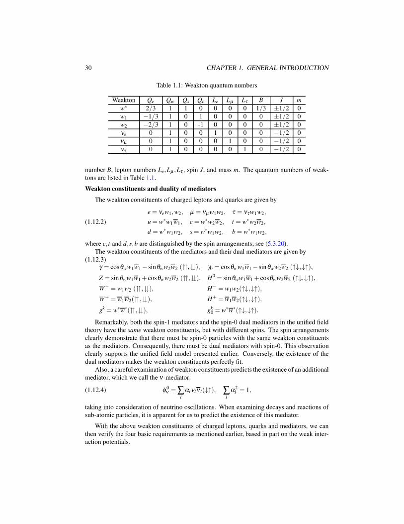
30 CHAPTER 1. GENERAL INTRODUCTION
Table 1.1: Weakton quantum numbers
Weakton Qe Qw Qs Qc Le Lµ Lτ B J m
w∗ 2/3 1 1 0 0 0 0 1/3 ±1/2 0
w1 −1/3 1 0 1 0 0 0 0 ±1/2 0
w2 −2/3 1 0 -1 0 0 0 0 ±1/2 0
νe 0 1 0 0 1 0 0 0 −1/2 0
νµ 0 1 0 0 0 1 0 0 −1/2 0
ντ 0 1 0 0 0 0 1 0 −1/2 0
number B, lepton numbers Le,Lµ ,Lτ , spin J, and mass m. The quantum numbers of weak-
tons are listed in Table 1.1.
Weakton constituents and duality of mediators
The weakton constituents of charged leptons and quarks are given by
(1.12.2)
e = νew1,w2, µ = νµ w1w2, τ = ντ w1w2,
u = w∗w1w1, c = w∗w2w2, t = w∗w2w2,
d = w∗w1w2, s = w∗w1w2, b = w∗w1w2,
where c, t and d,s,b are distinguished by the spin arrangements; see (5.3.20).
The weakton constituents of the mediators and their dual mediators are given by
(1.12.3)γ = cosθww1w1 − sinθww2w2 (,), γ0 = cosθww1w1 − sinθww2w2 (↑↓,↓↑),Z = sinθww1w1 + cosθww2w2 (,), H0 = sinθww1w1 + cosθww2w2 (↑↓,↓↑),W− = w1w2 (,), H− = w1w2(↑↓,↓↑),W+ = w1w2(,), H+ = w1w2(↑↓,↓↑),gk = w∗w∗(,), gk
0 = w∗w∗(↑↓,↓↑).Remarkably, both the spin-1 mediators and the spin-0 dual mediators in the unified field
theory have the same weakton constituents, but with different spins. The spin arrangements
clearly demonstrate that there must be spin-0 particles with the same weakton constituents
as the mediators. Consequently, there must be dual mediators with spin-0. This observation
clearly supports the unified field model presented earlier. Conversely, the existence of the
dual mediators makes the weakton constituents perfectly fit.
Also, a careful examination of weakton constituents predicts the existence of an additional
mediator, which we call the ν-mediator:
(1.12.4) φ0ν = ∑
l
αlνlν l(↓↑), ∑l
α2l = 1,
taking into consideration of neutrino oscillations. When examining decays and reactions of
sub-atomic particles, it is apparent for us to predict the existence of this mediator.
With the above weakton constituents of charged leptons, quarks and mediators, we can
then verify the four basic requirements as mentioned earlier, based in part on the weak inter-
action potentials.
1.12. WEAKTON MODEL OF ELEMENTARY PARTICLES 31
1. Mass generation. One important conclusion of the aforementioned weakton model is
that all particles—both matter particles and mediators—are made up of massless weaktons.
A fundamental question is how the mass of a massive composite particle is generated. In fact,
based on the Einstein formulas:
(1.12.5)d
dt~P =
√1− v2
c2~F , m =
√1− v2
c2
E
c2,
we observe that a particle with an intrinsic energy E has zero mass m = 0 if it moves in the
speed of light v = c, and possess nonzero mass if it moves with a velocity v < c. Hence by
this mass generation mechanism, for a composite particle, the constituent massless weaktons
can decelerate by the weak force, yielding a massive particle.
In principle, when calculating the mass of the composite particle, one should also con-
sider the bounding and repelling energies of the weaktons, each of which can be very large.
Fortunately, the constituent weaktons are moving in the “asymptotically-free” shell region of
weak interactions as indicated by the weak interaction potential/force formulas, so that the
bounding and repelling contributions to the mass are mostly canceled out. Namely, the mass
of a composite particle is due mainly to the dynamic behavior of the constituent weaktons.
2. Consistency and removal of unrealistic compositions. The consistency can be easily
checked. Also a few simple quantum rules can be devised so that unrealistic combinations of
weaktons are easily excluded.
3. The weakton confinement is simply the direct consequence of the weak interaction
potential/force formulas.
Mechanism of decays
Remarkably, the weakton model offers a perfect explanation for all sub-atomic decays. In
particular, all decays are achieved by 1) exchanging weaktons and consequently exchanging
newly formed quarks, producing new composite particles, and 2) separating the new compos-
ite particles by weak and/or strong forces.
One aspect of this decay mechanism is that we know now the precise constituents of
particles involved in all decays/reactions both before and after the reaction. It is therefore
believed that the new decay mechanism provides clear new insights for both experimental
and theoretical studies.
32 CHAPTER 1. GENERAL INTRODUCTION
Chapter 2
Fundamental Principles of Physics
The purposes of this chapter are 1) to provide an intuitive introduction to fundamental princi-
ples of Nature, and 2) to explain how the laws of Nature are derived based on these principles.
The main focus is on the symbiotic interplay between advanced mathematics and the laws of
Nature. For this purpose, we start with a brief overview on the perspective and the physical
significance of a few fundamental principles.
Section 2.1 provides a basic intuitive introduction to fundamental principles, symmetries,
the geometric interaction mechanism and the symmetry-breaking principle. We start with two
guiding principles of theoretical physics, which can be synthesized as: the laws of Nature are
represented by mathematical equations, are dictated by a few fundamental principles, and
always take the simplest and aesthetic forms.
The geometric interaction mechanism was originally motivated by Albert Einstein’s vi-
sion revealed in his principle of equivalence, and was first postulated in (Ma and Wang,
2014d).
Symmetry plays a fundamental role in physics. Many, if not all, physical systems obey
certain symmetry. For this reason, many fundamental principles in physics address the un-
derlying symmetries of physical systems.
However, a crucial component of the unification of four fundamental interactions as
well as the modeling of multi-level physical systems is the symmetry-breaking mechanism.
Consequently, we postulated in (Ma and Wang, 2014a) and in Section 2.1.7 a Principle of
symmetry-breaking 2.14, which states that for a system coupling different levels of physical
laws, part of these symmetries of the subsystems must be broken.
Section 2.2 addresses essentials of the classical Lorentz invariance, and its applications to
the derivation of Schrodinger equation, the Klein-Gordon equation, the Weyl equations and
the Dirac equations in relativistic quantum mechanics.
Section 2.3 presents a brief introduction to the Einstein theory of general relativity, fo-
cusing on Einstein’s two basic principles, the principle of equivalence and the principle of
general relativity, and on the derivation of the Einstein gravitational field equations.
A brief introduction to both the U(1) abelian and the SU(N) non-abelian gauge theories
are presented in Section 2.4. In particular, the U(1) abelian gauge theory is defined on the
33
34 CHAPTER 2. FUNDAMENTAL PRINCIPLES OF PHYSICS
complex spinor bundle M 4 ⊗p C4. The SU(N) non-abelian gauge theory, also called the
Yang-Mills theory, is the connection on the complex spinor bundle M 4 ⊗p (C4)N . Note that
the presentation here leads clearly to PRI, to be introduced in Chapter 4.
Section 2.5 introduces the principle of Lagrangian dynamics (PLD) and its many appli-
cations such as in classical mechanics and electrodynamics. The Noether Theorem, Theo-
rem 2.38, is also proved.
Section 2.6 is on Hamiltonian dynamics and its connections to the Lagrangian dynamics.
2.1 Essence of Physics
2.1.1 General guiding principles
Physics studies fundamental interactions, motion and formation of matter in our Universe.
The heart of fundamental physics is to seek experimentally verifiable, fundamental laws and
principles of Nature. Namely, physical concepts and theories are transformed into mathemat-
ical models, and the predictions derived from these models can be verified experimentally
and conform to the reality.
Modeling is a crucial step to understand a physical phenomena. A good model should be
derived based on a few fundamental principles, and often presented in the form of differen-
tial equations. The first principles are often connected with symmetries, which also dictate
specific forms of mathematical models, represented by differential equations.
In a nutshell, we have the following first principle of physics.
First Principle of Physics 2.1. Physical systems obey laws and principles of Nature:
1) These laws and principles can be expressed using mathematical models:
Model = Mathematical representation of physical laws and principles;
2) These laws and principles are universal, and the universality is reflected by symmetries
in physics; and
3) Physical symmetries dictate the precise forms of the mathematical models, which are
often presented in the forms of ordinary or partial differential equations.
In addition, the following principle provides the essence of fundamental physics, and is
supported by known experimental facts.
Essence of Physics 2.2. The essence of physics can be drawn in the following two important
ingredients:
1) Theoretical physics is built upon a few fundamental principles of Nature; and
2) The laws of Nature always take the simplest and aesthetic forms.
First Principle 2.1 and Essence of Physics 2.2 serve as guiding principles to understand
and explore the physical world of our Universe and the laws of Nature.
2.1. ESSENCE OF PHYSICS 35
2.1.2 Phenomenological methods
Theories of physics fall into two categories: first principle theories and phenomenological
theories. The first principle theories are derived based on a few fundamental laws and princi-
ples of Nature, and phenomenological theories are conjectured and synthesized from obser-
vational data.
For example, the Newton’s gravitational law is given by
(2.1.1) F =−m1m2G
r2.
which is essentially deduced by using the phenomenological technique based on a large num-
ber of astronomical data. First, one readily conjectures that the gravitational force is propor-
tional to the masses m and M of the two bodies, and is a function of distance r:
F =−mMΦ(r),
where Φ(r) is an undetermined function.
Then one considers two planets with masses m1 and m2, rotating around the Sun with
velocities v1 and v2. By the balance between the gravitational and centrifugal forces, we have
v2i
ri
= MΦ(ri) for i = 1,2,
where M is the mass of the Sun. Consequently,
(2.1.2)Φ(r1)
Φ(r2)=
r2
r1
v21
v22
.
By the Kepler Third Law, the periods T1 and T2 of the two planets satisfy
T 21
T 22
=r3
1
r32
, Tivi = 2πri for i = 1,2,
which implies that
(2.1.3)v2
1
v22
=r2
r1
.
Then, it follows from (2.1.2) and (2.1.3) that
Φ(r) =G
r2,
where G is a constant, called the gravitational constant. Thus, by the Kepler Third Law, one
can postulate naturally the Newtonian gravitational law (2.1.1). In other words, the Newto-
nian Gravitational Law can be regarded as a phenomenological theory.
Albert Einstein was the first who tried to deduce basic physical laws from first principles.
For example, the Einstein theory of general relativity and the Einstein gravitational field
equations:
(2.1.4) Rµν −1
2gµνR =−8πG
c4Tµν ,
are derived based on the following three basic principles:

36 CHAPTER 2. FUNDAMENTAL PRINCIPLES OF PHYSICS
1) the principle of general relativity,
2) the principle of equivalence, and
3) the principle of Lagrangian dynamics.
The Schwarzschild solution of the Einstein gravitational field equations (2.1.4) offers a natu-
ral link between the field equations and the Newtonian gravitational law (2.1.1).
2.1.3 Fundamental principles in physics
Fundamental first principles refer to the laws of Nature that cannot be derived from other
more basic laws.
Based on Essence of Physics 2.2, if we would like to better understand theoretical physics,
it is crucial to know and find out all fundamental laws. In this subsection, we shall list the
known and important principles in various physical fields, most of which will be introduced
in later chapters.
We start with the introduction of Principle of Lagrangian Dynamics (PLD), which is of
special importance.
In classical mechanics, we know the least action principle. For a mechanical system with
the position and velocity variables
(2.1.5) x = (x1, · · · ,xn), x = (x1, · · · , xn),
let the kinetic energy T and the potential energy V be functions of the position and velocity
variables in (2.1.5). Then the states of the system are the extremum points of the functional
(2.1.6) L(x) =∫ t1
t0
L (x, x)dt,
where the integrand L
(2.1.7) L (x, x) = T −V.
is called the Lagrange density, and the functional (2.1.6) is called the Lagrange action. The
extremum points x satisfy the variational equation, called the Euler-Lagrange equations of
(2.1.6):
(2.1.8) δL(x) = 0,
where δL is the variational derivative operator of L. The equation (2.1.8) can be equivalently
expressed asd
dt
∂L
∂ x− ∂L
∂x= 0.
The most important point is that the least action principle can be generalized to all phys-
ical systems describing motions, as well as to fundamental interactions of Nature. The gen-
eralization in a motion system is called the PLD, and in an interaction system is called the
Principle of Interaction Dynamics (PID). PID will be introduced in detail In Chapter 4 of this
book, and PLD is stated as follows.
2.1. ESSENCE OF PHYSICS 37
Principle of Lagrangian Dynamics 2.3. For a physical motion system, there are functions
(2.1.9) u = (u1, · · · ,un),
which describe the states of this system, and there exists a functional of u, given by
(2.1.10) L(u) =∫
ΩL (u,Du, · · · ,Dmu)dx,
where Ω is the domain of u, and Dku is the k-th derivative of u for any 0 ≤ k ≤ m. Then the
state functions of this system are the extremum points of (2.1.10). Namely the state functions
satisfy the variational equation of (2.1.10):
(2.1.11) δL(u) = 0.
The functional L is called the Lagrange action, and L is called the Lagrange density.
By PLD, to derive dynamical equations for a physical system, it suffices to find the corre-
sponding Lagrange action. In the next subsection, we demonstrate that symmetries in physics
dictate the precise forms of the Lagrange actions.
A list of known important physical principles and laws of Nature in various subfields of
physics is given as follows.
1) Universal principles in all fields:
• Principle of Lagrangian Dynamics (PLD),
• Principle of Hamiltonian Dynamics (PHD),
• Principle of Interaction Dynamics (PID),
• Lorentz Invariance,
• Principle of General Relativity,
• Principle of Gauge Invariance,
• Principle of Representation Invariance (PRI),
• Principle of Symmetry-Breaking
2) Classical mechanics:
• Newtonian Second Law,
• Principle of Least Action,
• Principle of Galilean Invariance,
• Fick and Fourier Diffusion Laws.
3) Quantum physics:
• Basic postulates of quantum physics,
• Pauli Exclusion Principle.
4) Statistical physics:
38 CHAPTER 2. FUNDAMENTAL PRINCIPLES OF PHYSICS
• Basic Laws of Thermodynamics,
• Le Chaterlier Principle.
5) Nonlinear sciences:
• Principle of Phase Transition Dynamics.
A couple of remarks are now in order.
Remark 2.4. Because various conservation laws can be deduced by PHD, PLD and sym-
metries based on the Noether theorem, these laws are not listed in the fundamental princi-
ples.
Remark 2.5. Mathematical models form the skeleton of theoretical physics, and most, if not
all, mathematical models (differential equations) in theoretic physics can be derived based on
the principles listed above. One of the ultimate goals of this book is to derive physical models
based on a first principles.
2.1.4 Symmetry
Symmetry plays an important role in physics. We start with intuitively examining how sym-
metry works, keeping in mind the relation between equations and laws of physics in First
Principle 2.1, which can be simply recast as
(2.1.12) Laws of Physics = Differential Equations.
The laws of Nature on the left hand side of (2.1.12) are often beyond words, and are
best expressed by differential equations. It is this characteristic, together with the Noether
theorem, that illustrates the importance of symmetry in physics, as illustrated below:
Invariance Covariance Symmetry
⇓ ⇓ ⇓Form of Equation Space Structure Conservation Law
Namely, symmetry dictates and determines
1) the explicit form of differential equations governing the underlying physical system,
2) the space-time structure of the Universe, and the mechanism of fundamental interac-
tions of Nature, and
3) physical conservation laws.
We now give a simple example to demonstrate how symmetry determines the explicit
form of equations. We begin with two basic implications of a symmetry:
a) Fundamental laws of Nature are universal, and their validity is independent of the
space, time, and directions of experiments and observations, and
2.1. ESSENCE OF PHYSICS 39
b) By (2.1.12), the universality of laws of Nature implies that the differential equations
representing them are covariant. Equivalently the Lagrange actions are invariant under
the corresponding coordinate transformations.
As an example, consider a physical system obeying PLD 2.3. For simplicity, we assume
that the Lagrange action of this fictitious system is finite-dimensional. Namely, let
F : Rn → R1
be a finite dimensional function regarded as the action of the physical system, and we need
to determine the explicit form of this function
(2.1.13) F = F(x) for x = (x1, · · · ,xn) ∈Rn.
Consider the case where the system satisfies the following invariance principle, called the
principle of rotational invariance.
Principle 2.6 (Rotational Invariance). The laws that the system (2.1.13) obeys are the same
under all orthogonal coordinate systems.
Based on the implication b) of symmetry above, Principle of Rotational Invariance 2.6
says that the action (2.1.13) is invariant under orthogonal coordinate transformations:
(2.1.14) x = Ax where A is an arbitrary orthogonal matrix.
We know that the two forms as
|x|2 = x21 + · · ·+ x2
n, x · y = x1y1 + · · ·+ xnyn
are invariant, where y ∈Rn is given, and the invariant function F(x) must be of the form:
F(x) = F(|x|, x · y)
In addition, by the simplicity principle in Essence of Physics 2.2, the exponent of F in x is
two. Thus the action (2.1.13) is defined in the form as
(2.1.15) F(x) = α|x|2 +β x · y,
where α,β are two constants, and y is a given vector.
Thus we deduce an explicit expression (2.1.15) for the function F , which are invariant
under rotational symmetry, Principle 2.6. The graph of (2.1.15) is a sphere, and the invariance
of (2.1.15) means that the sphere looks the same from different directions. This is the reason
why an invariance is called a symmetric principle.
2.1.5 Invariance and tensors
Symmetries are characterized by three ingredients:
spaces, transformation groups, and tensors,
40 CHAPTER 2. FUNDAMENTAL PRINCIPLES OF PHYSICS
which are applicable to different physical fields. Here are the five currently known important
symmetries and their corresponding ingredients:
1) Galileo Invariance:
• Space: Euclidean space R3,
• Transformation group: Galileo group and SO(3),
• Tensor types: Cartesian tensors,
• Fields: classical mechanics, fluid dynamics, and astrophysics.
2) Lorentz Invariance:
• Space: Minkowski space,
• Transformation group: Lorentz groups,
• Tensor types: 4-dimensional tensors and spinors,
• Fields: Quantum physics and Interactions.
3) Einstein General Relativity:
• Space: 4-dimensional Riemann manifolds,
• Transformation group: GL(4),
• Tensor types: General tensors and Riemann metric,
• Fields: Gravitation and Astrophysics.
4) Gauge Invariance:
• Space: complex vector bundle M ⊗p Cn,
• Transformation groups: U(1) and SU(n),
• Tensor types: Wave functions and gauge fields,
• Fields: Quantum physics and Interactions.
5) Representation Invariance:
• Space: Tangent space of SU(n),
• Transformation: GL(Cn),
• Tensor types: SU(n) tensors,
• Fields: Quantum physics and Interactions.
We now use examples in classical mechanics to illustrate the main characteristics of these
symmetries and to clarify how tensors describe invariances.
Principle 2.7 (Galilean Invariance). Mechanical laws are invariant under the following trans-
formations:
2.1. ESSENCE OF PHYSICS 41
1) Galilean transformation
(2.1.16) t = t, x = x+ vt for x ∈R3,
where v is a constant velocity, and
2) translational and rotational transformations
(2.1.17) t = t + t0, x = Ax+ b for x ∈ R3,
where A ∈ SO(3) is an orthogonal matrix, b ∈ R3 and t0 ∈ R1 are constant.
By (2.1.12) we know that the invariance of physical laws is equivalent to the covariance
of the corresponding differential equations. We now demonstrate that the Newton Second
Law obeys the Galileo Invariance Principle 2.7.
The Newton Second Law reads as
(2.1.18) ma = F,
and the corresponding differential equation describing the motion of a particle is given by
(2.1.19) md2x
dt2= F.
When we investigate the motion in other reference frame (x, t) with the transformation
(2.1.20) t = t + t0, x = Ax+ vt+ b,
by (2.1.20) we derive
(2.1.21)d2x
dt2= A
d2x
dt2.
On the other hand, experiments show that the expressions F in (x, t) and F in (x, t) of force
satisfy the relation:
(2.1.22) F = AF.
Hence, by (2.1.19) we deduce from (2.1.21) and (2.1.22) that
(2.1.23) md2x
dt2= F .
It is clear that both forms of (2.1.19) and (2.1.23) are the same under the transformation
(2.1.20), i.e. under the transformations (2.1.16) and (2.1.17).
Mathematically, the transformations corresponding to (2.1.16) and (2.1.17) are the Galileo
group and SO(3), and the functions satisfying (2.1.21) and (2.1.22) under the transformation
(2.1.20) are called first-order Cartesian tensors, which are also the usual vectors in R3.
Also, this example demonstrates that invariance principles must be characterized by cor-
responding tensors. In the later sections, we shall give precise definitions of various types of
tensors.
42 CHAPTER 2. FUNDAMENTAL PRINCIPLES OF PHYSICS
Remark 2.8. In classical mechanics, the laws were first discovered phenomenologically, and
then were known to obey the Galileo Principle of Invariance. It is Einstein’s vision that laws
of physics can be derived from symmetries.
Remark 2.9. The transformation (2.1.17) consists of three subclasses of transformations:
(2.1.24)
the rotation transformation: x = Ax,
the space translation: x = x+ b,
the time translation: t = t + t0.
Unlike the Galileo Invariance of (2.1.16), which is only valid in the classical mechanics,
the invariance for the transformations (2.1.24) are universally valid in all physical fields.
In particular, based on the Noether Theorem, Theorem 2.38, we can deduce the following
corresponding conservation laws:
Time translation invariance ⇒ Energy conservation,
Space translation invariance ⇒ Momentum conservation,
Rotational invariance ⇒ Angular momentum conservation.
2.1.6 Geometric interaction mechanism
Albert Einstein was the first physicist who postulated that the gravitational force is caused by
the time-space curvature. However, Yukawa’s viewpoint, entirely different from Einstein’s,
is that the other three fundamental forces take place through exchanging intermediate bosons
such as photons for the electromagnetic interaction, W± and Z intermediate vector bosons
for the weak interaction, and gluons for the strong interaction.
Based on our recent studies on field theory of the four interactions, in the same spirit as
the Einstein’s mechanism of gravitational force, it is natural for us to postulate a mechanism
for all four interactions different from that of Yukawa.
To proceed, we recall that in geometry, the square ds2 of an infinitesimal arc-length in a
flat space can be written as
ds2 = dx21 + · · ·+ dx2
n,
which is the well known Pythagorean theorem, and in a curved space ds2 is given by
(2.1.25) ds2 = gi j(x)dxidx j with gi j 6= δi j ,
and the Pythagorean theorem is in general not true in a curved space. Mathematically, a space
M being flat indicates that one can choose properly a coordinate system so that the metric
gi j = δi j,
and otherwise, M will be curved.
Regarding to the laws of Nature on our Universe M , physical states are described by
functions u = (u1, · · · ,un) defined on M :
u : M → M ⊗p Rn for non-quantum system,(2.1.26)
u : M → M ⊗p Cn for quantum system,(2.1.27)
2.1. ESSENCE OF PHYSICS 43
which are solutions of differential equations associated with the laws of the underlying phys-
ical system:
(2.1.28) δL(Du) = 0,
where D is a derivative operator, and L is the Lagrange action. Consider two transformations
for the two physical systems (2.1.26) and (2.1.27):
x = Tx for (2.1.26),(2.1.29)
u = eiθτ u for (2.1.27),(2.1.30)
where x is a coordinate system in M , T : Rn →Rn is a linear transformation, eiθτ : Cn →Cn
is an SU(n) transformation, θ is a function of x, and τ is a traceless Hermitian matrix; see
Section 2.4 on gauge theory.
We now state two important symmetric principles: the Einstein principle of general rela-
tivity and the gauge invariance.
Principle 2.10 (General Relativity). Laws of Physics are the same under all coordinate sys-
tems. Namely, equations (2.1.28) are covariant and equivalently the action L is invariant
under all coordinate transformations (2.1.29).
Principle 2.11 (Gauge Invariance). A quantum system with electromagnetic, weak, and strong
interactions is invariant under the corresponding SU(n) gauge transformations (2.1.30).
One important consequence of the invariance of (2.1.28) under the transformations (2.1.29)
and (2.1.30) is that the derivatives D in (2.1.28) must take the following form (see Section
2.4 for detailed derivations):
D = ∇+Γ for (2.1.26),(2.1.31)
D = ∇+ igAτ for (2.1.27),(2.1.32)
where Γ depends on the metrics gi j, A is a gauge field, representing the interaction potential,
and g is the coupling constant, representing the interaction charge.
The derivatives defined in (2.1.31) and (2.1.32) are called connections respectively on M
and on the complex vector bundle M ⊗p Cn. For the connections, we have the following
theorem, providing a mathematical basis for our interaction mechanism.
Theorem 2.12.
1) The space M is curved if and only if Γ 6= 0 in all coordinates, or equivalently gi j 6= δi j
under all coordinate systems;
2) The complex bundle M ⊗pCn is geometrically nontrivial or twisted if and only if A 6= 0.
Consequently, by Principle 2.10, the presence of the gravitational field implies that the
space-time manifold is curved, and, by Principle 2.11, the presence of the electromagnetic,
the weak and strong interactions indicates that the complex vector bundle M ⊗pCn is twisted:
(2.1.33)Principle 2.10 ⇒ gi j 6= δi j ⇒ M is curved,
Principle 2.11 ⇒ A 6= 0 ⇒ M ⊗p Cn is twisted.
This analogy, together with Einstein’s vision on gravity as the curved effect of space-time
manifold, it is natural for us to postulate the following mechanism for all four interactions.
44 CHAPTER 2. FUNDAMENTAL PRINCIPLES OF PHYSICS
Geometric Interaction Mechanism 2.13. The gravitational force is the curved effect of the
time-space, and the electromagnetic, weak, strong interactions are the twisted effects of the
underlying complex vector bundles M ⊗p Cn.
As mentioned earlier, traditionally one adopts Yukawa’s viewpoint that forces of the in-
teractions of Nature are caused by exchanging the field mediators. Namely, the gravitation
is due to exchanging gravitons, the electromagnetic force is due to exchanging photons, the
weak force is due to exchanging the intermediate vector bosons, and the strong force is due
to exchanging gluons. The point of view we are taking is the Interaction Mechanism 2.13,
following Einstein’s version.
2.1.7 Principle of symmetry-breaking
Different physical systems obey different physical principles. The four fundamental inter-
actions of Nature, the quantum systems, the fluid dynamics and heat conduction obey the
following symmetry principles:
(2.1.34)
the general relativity for gravity,
the Lorentz and gauge invariances for the other three interactions,
the Lorentz invariance for quantum systems, and
the Galilean invariance for fluid and heat conductions.
The corresponding fields and systems in (2.1.34) are governed by the following physical laws
and first principles:
(2.1.35)
PID and PRI for four fundamental interactions,
PLD for quantum systems,
the Newton Second Law for fluids,
diffusion laws for heat conductivity,
Here PID stands for the principle of interaction dynamics, and PRI stands for the principle
of representation invariance, both discovered recently by the authors. PLD stands for the
principle of Lagrangian dynamics.
Astrophysics is the only field that involving all the fields in (2.1.34) and (2.1.35). Conse-
quently, one needs to couple the basic laws in (2.1.35) to model astrophysical dynamics.
One difficulty we encounter now is that the Newtonian Second Law for fluid motion
and the diffusion law for heat conduction are not compatible with the principle of general
relativity. Also, there are no basic principles and rules for combining relativistic systems and
the Galilean systems together to form a consistent system. The reason is that in a Galilean
system, time and space are independent, and physical fields are 3-dimensional; while in a
relativistic system, time and space are related, and physical fields are 4-dimensional.
The distinction between relativistic and Galilean systems gives rise to an obstacle for
establishing a consistent model of astrophysical dynamics, coupling all the physical systems
in (2.1.34) and (2.1.35).
In the unified field theory based on PID, the key ingredient for coupling gravity with
the other three fundamental interactions is achieved through spontaneous gauge symmetry
2.1. ESSENCE OF PHYSICS 45
breaking. Here we propose that the coupling between the relativistic and the Galilean systems
through relativistic-symmetry breaking.
In fact, the model given by (7.1.75)-(7.1.76) follows from this symmetry-breaking prin-
ciple, where we have to chose the coordinate system
xµ = (x0,x), x0 = ct and x = (x1,x2,x3),
such that the metric is in the form:
(2.1.36) ds2 =−(
1+2
c2φ(x, t)
)c2dt2 + gi j(x, t)dxidx j.
Here gi j (1 ≤ i, j ≤ 3) are the spatial metric, and
(2.1.37) φ = the gravitational potential.
With this metric (2.1.36)-(2.1.37), we can establish the fluid and heat equations as in (7.1.78).
It is then clear that by fixing the coordinate system to ensure that the metric is in the form
(2.1.36)-(2.1.37), the system breaks the symmetry of general coordinate transformations, and
we call such symmetry-breaking as relativistic-symmetry breaking.
We believe the symmetry-breaking is a general phenomena when we deal with a physical
system coupling different subsystems in different levels. The unified field theory for the four
fundamental interactions is a special case, which couples the general relativity, the Lorentz
and the gauge symmetries. Namely, the symmetry of general relativity needs to be linked to
both the Lorentz invariance and the gauge invariance in two aspects as follows:
1) In the Dirac equations for the fermions:
iγµDµ ψ − c
hmψ = 0,
γµ have to obey two different transformations.
2) The gauge-symmetry breaks in the gravitational field equations coupling the other in-
teractions:
(2.1.38) Rµν −1
2gµνR =−8πG
c4Tµν +DµΦν ,
where
(2.1.39) Dµ = ∇µ +k1
hceAµ +
k2
hcgwWµ +
k3
hcgsSµ ,
∇µ is the covariant derivative, ki (1 ≤ i ≤ 3) are parameters, Aµ ,Wµ ,Sµ are the total
electromagnetic, weak and strong interaction potentials. It is the terms Aµ ,Wµ ,Sµ in
(2.1.39) that break the gauge symmetry of (2.1.38).
In summary, we are ready to postulate a general symmetry-breaking principle.
Principle of Symmetry-Breaking 2.14.
46 CHAPTER 2. FUNDAMENTAL PRINCIPLES OF PHYSICS
1) The three sets of symmetries,
(2.1.40)
the general relativistic invariance,
the Lorentz and gauge invariances, and
the Galileo invariance,
are mutually independent and dictate in part the physical laws in different levels of
Nature; and
2) for a system coupling different levels of physical laws, part of these symmetries must
be broken.
This principle of symmetry-breaking holds the key component for us to establish the
PID unified field theory for four fundamental interactions in Chapter 4, the field equations
for multi-particle systems in Chapter 6, and the astrophysical fluid dynamical equations in
Chapter 7, resolving a number of important physical problems.
2.2 Lorentz Invariance
2.2.1 Lorentz transformation
In 1903, H. A. Lorentz discovered the Lorentz coordinate transformation, under which the
laws of electromagnetism are invariant. Consequently, physicists discovered two different
invariances:
the Galilean invariance in classical mechanics,(2.2.1)
the Lorentz invariance in electromagnetism.(2.2.2)
In 1905, Albert Einstein introduced the special theory of relativity, based on the following
two first principles: the principle of special relativity and the principle of invariance of the
speed of light.
Principle 2.15 (Special Relativity). Physical laws are covariant in all inertial systems.
Principle 2.16 (Invariance of speed of light). The vacuum speed of light is a universal con-
stant.
A few remarks are now in order. First, a system of reference is always needed to describe
the nature, and an inertial system is a system on which a freely moving object moves with
constant velocity (Landau and Lifshitz, 1975). Second, it is clear that under the Galilean
invariance, the speed of light changes in different inertial systems. Consequently, the Galilean
invariance and the Lorentz invariance are incompatible. Third, the invariance of the vacuum
speed of light was verified by the Michelson and Morley experiment. Einstein discovered
his special theory of relativity by postulating, based on Principles 2.15-2.16, the following
principle of Lorentz invariance.
Principle 2.17 (Lorentz Invariance). Physical laws are invariant under Lorentz transforma-
tions.
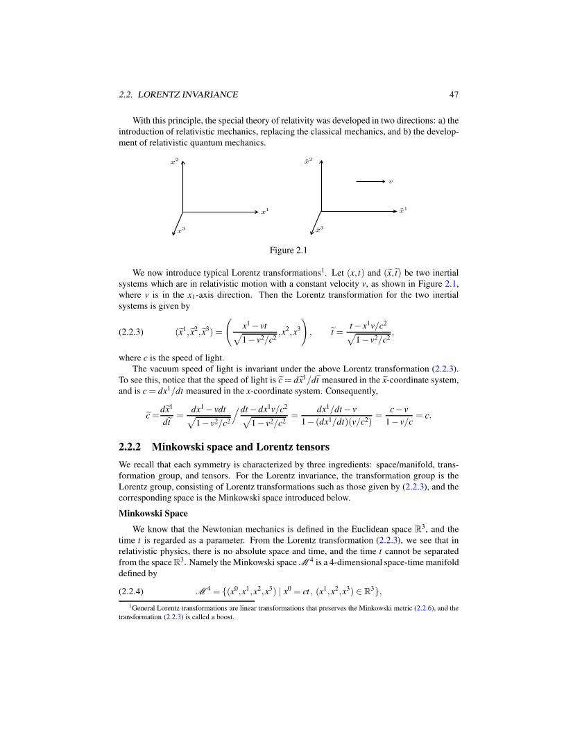
2.2. LORENTZ INVARIANCE 47
With this principle, the special theory of relativity was developed in two directions: a) the
introduction of relativistic mechanics, replacing the classical mechanics, and b) the develop-
ment of relativistic quantum mechanics.
x1
x2
x3
x1
x2
x3
v
Figure 2.1
We now introduce typical Lorentz transformations1. Let (x, t) and (x, t) be two inertial
systems which are in relativistic motion with a constant velocity v, as shown in Figure 2.1,
where v is in the x1-axis direction. Then the Lorentz transformation for the two inertial
systems is given by
(2.2.3) (x1, x2, x3) =
(x1 − vt√1− v2/c2
,x2,x3
), t =
t − x1v/c2
√1− v2/c2
,
where c is the speed of light.
The vacuum speed of light is invariant under the above Lorentz transformation (2.2.3).
To see this, notice that the speed of light is c = dx1/dt measured in the x-coordinate system,
and is c = dx1/dt measured in the x-coordinate system. Consequently,
c =dx1
dt=
dx1 − vdt√1− v2/c2
/dt − dx1v/c2
√1− v2/c2
=dx1/dt − v
1− (dx1/dt)(v/c2)=
c− v
1− v/c= c.
2.2.2 Minkowski space and Lorentz tensors
We recall that each symmetry is characterized by three ingredients: space/manifold, trans-
formation group, and tensors. For the Lorentz invariance, the transformation group is the
Lorentz group, consisting of Lorentz transformations such as those given by (2.2.3), and the
corresponding space is the Minkowski space introduced below.
Minkowski Space
We know that the Newtonian mechanics is defined in the Euclidean space R3, and the
time t is regarded as a parameter. From the Lorentz transformation (2.2.3), we see that in
relativistic physics, there is no absolute space and time, and the time t cannot be separated
from the space R3. Namely the Minkowski space M 4 is a 4-dimensional space-time manifold
defined by
(2.2.4) M4 = (x0,x1,x2,x3) | x0 = ct, (x1,x2,x3) ∈ R
3,1General Lorentz transformations are linear transformations that preserves the Minkowski metric (2.2.6), and the
transformation (2.2.3) is called a boost.
48 CHAPTER 2. FUNDAMENTAL PRINCIPLES OF PHYSICS
where c is the speed of light, and M 4 is endowed with the Riemannian metric:
(2.2.5) (gµν) =
−1 0 0 0
0 1 0 0
0 0 1 0
0 0 0 1
.
The doublet M 4,gµν given by (2.2.4) and (2.2.5) is called the Minkowski space, and the
metric (2.2.5) can be equivalently expressed in the form
(2.2.6) ds2 = gµνdxµdxν =−c2dt2 + dx2 =−c2dt2 +(dx1)2 +(dx2)2 +(dx3)2.
Lorentz transformations are linear transformations of the Minkowski space M 4 that pre-
serve the metric (2.2.6). The following coordinate transformation of the Minkowski space is
a Lorentz transformation, called boost, corresponding to Figure 2.1:
(2.2.7)
x0
x1
x2
x3
=
1√1−β 2
− β√1−β 2
0 0
− β√1−β 2
1√1−β 2
0 0
0 0 1 0
0 0 0 1
x0
x1
x2
x3
,
where β = ν/c. Both transformations (2.2.3) and (2.2.7) are the same in form, but the mathe-
matical implication is changed. Here, (2.2.7) represents the coordinate transformation for the
Minkowski space M 4. With Einstein’s summation convention, (2.2.7) is often denoted by
(2.2.8) xµ = Lµν xν ,
where
(2.2.9) (Lµν ) =
1√1−β 2
− β√1−β 2
0 0
− β√1−β 2
1√1−β 2
0 0
0 0 1 0
0 0 0 1
is the Lorentz matrix, and its inverse (lµν ) = (L
µν )
−1 is given by
(2.2.10) (lµν ) =
1√1−β 2
β√1−β 2
0 0
β√1−β 2
1√1−β 2
0 0
0 0 1 0
0 0 0 1
.
An important property of the Minkowski space is that its Riemannian metric is invariant
under the Lorentz transformation (2.2.7).
2.2. LORENTZ INVARIANCE 49
Theorem 2.18. The Minkowski metric (2.2.5) or (2.2.6) is invariant under the coordinate
transformation (2.2.7). Namely the metric (gµν ) in xµ is the same as that in xµ:
(2.2.11) (gµν) = (gµν).
In other words, ds2 in xµ is also expressed as
ds2 =−c2dt2 + dx2, x = (x1, x2, x3).
The proof of Theorem 2.18 needs to use the properties of tensors. In fact, the Minkowski
metric (2.2.5) is a second-order covariant Lorentz tensor, i.e. under the transformation (2.2.8),
gµν transforms as
(2.2.12) (gµν) = (lαβ )(gµν)(l
αβ )
T ,
where (lµµ ) is the inverse of (L
µν ) given by (2.2.10). Then, a direct computation we can get
(2.2.11) from (2.2.12).
Lorentz Transformation Group
Each transformation (2.2.8) corresponds to a Lorentz matrix (Lµν ) given by (2.2.9). These
matrices constitute a group in the multiplication as
1√1−β 2
− β√1−β 2
0 0
− β√1−β 2
1√1−β 2
0 0
0 0 1 0
0 0 0 1
1√1−γ2
− γ√1−γ2
0 0
− γ√1−γ2
1√1−γ2
0 0
0 0 1 0
0 0 0 1
=
1√1−α2
− α√1−α2
0 0
− α√1−α2
1√1−α2
0 0
0 0 1 0
0 0 0 1
,
where
β =v
c, γ =
u
c, α =
w
c, w =
u+ v
1+ uv/c2,
where w is the velocity composed by u and v by the theory of special relativity.
Thanks to Theorem 2.18, we can define Lorentz transformation group as all linear trans-
formations of the Minkowski space M 4, that preserve the Minkowski metric; see (2.2.12):
(2.2.13) LG = (Lµν ) : M
4 → M4 | (gµν) = (Lα
β )(gµν )(Lαβ )
T , det(Lµν ) = 1.
Elements of LG are also called Lorentz matrices, and relativistic physics is referred to the
invariance of action under the Lorentz group. The invariance of the Minkowski metric implies
the Lorentz invariance of physical laws.
In this definition, we require det(Lµν ) = 1, and such transformations are often called
proper Lorentz transformation in physics literatures. The parity transformation and time re-
versal are two special linear transformations of the Minkowski space, which are not elements
in LG as defined in (2.2.13) and are often dealt with separately:
(2.2.14) P =
1 0 0 0
0 −1 0 0
0 0 −1 0
0 0 0 −1
, T =
−1 0 0 0
0 1 0 0
0 0 1 0
0 0 0 1
.
50 CHAPTER 2. FUNDAMENTAL PRINCIPLES OF PHYSICS
Lorentz Tensors
We now define Lorentz tensors, also called 4-dimensional (4-D) tensors, corresponding
to the Lorentz invariance.
Definition 2.19 (Lorentz Tensors). The following quantities are called Lorentz tensors, or
4-dimensional tensors:
1) A function T with 4k components
T = Tµ1···µk, µ1, · · · ,µk = 0,1,2,3,
is called a k-th order covariant tensor, if under the Lorentz transformation (2.2.13), the
components of T transform as
Tµ1···µk= l
ν1µ1· · · lνk
µkTν1···νk
,
where (lνµ) = (L
µν )
−1 is the inverse transformation of the Lorentz transformation (Lµν )∈
LG.
2) A tensor
T = T µ1···µk, µ1, · · · ,µk = 0,1,2,3,
is called a k-th order contra-variant tensor, if under the Lorentz transformation (Lµν ) ∈
LG, the components of T change as
T µ1···µk = Lµ1ν1· · ·Lµk
νkT ν1···νk .
3) A function
T = Tµ1···µr
ν1···νs, r+ s = k,
is called a k-th order (r,s)-type tensor, if under the Lorentz transformation (Lµν ) ∈ LG,
Tµ1···µr
ν1···νs= l
α1ν1
· · · lαsνs
Lµ1
β1· · ·Lµr
βrT
β1···βrα1···αs
.
In physics, the most important tensors are first- and second-order tensors. The following
is a list of commonly encountered 4-D tensors, and we always use (gµν) = (gµν)−1 with
(gµν ) being the Minkowski metric given by (2.2.5):
1) Position vectors:
(2.2.15)xµ = (x0,x1,x2,x3), x0 = ct,xµ = (x0,x1,x2,x3) = gµνxν = (−x0,x1,x2,x3).
2) The 4-D electromagnetic potential:
(2.2.16)Aµ = (A0,A1,A2,A3),Aµ = (A0,A1,A2,A3) = gµνAν ,
where A0 = −A0 is the electric potential, (A1,A2,A3) = (A1,A2,A3) is the magnetic
vector potential.
2.2. LORENTZ INVARIANCE 51
3) The 4-D current density:
(2.2.17)Jµ = (J0,J1,J2,J3),Jµ = (J0,J1,J2,J3) = gµνJν ,
where J0 =−J0 = cρ , ρ is the charge density, and ~J = (J1,J2,J3) is the current density
field.
4) The 4-D energy-momentum vector:
(2.2.18)Eµ = (E,cP1,cP2,cP3),Eµ = gµνEν = (−E,cP1,cP2,cP3),
where E is the energy, and P = (P1,P2,P3) is the momentum vector,
5) The 4-D gradient operators:
(2.2.19)
∂µ =
(∂
∂x0,
∂
∂x1,
∂
∂x2,
∂
∂x3
)=
(1
c
∂
∂ t,∇
),
∂ µ = gµν∇µ =
(− ∂
∂x0,
∂
∂x1,
∂
∂x2,
∂
∂x3
)=
(−1
c
∂
∂ t,∇
),
transform as the first-order Lorentz tensors.
2.2.3 Relativistic invariants
All Lagrange actions in relativistic physics are Lorentz invariants. The most common Lorentz
invariants are contractions of 4-D tensors. For example, let
Aµ = (A0,A1,A2,A3), Bµ = (B0,B1,B2,B3)
be the covariant and contra-variant vectors. Then the contraction
(2.2.20) AµBµ = A0B0 +A1B1 +A2B2 +A3B3
is a Lorentz invariant. In fact, under the Lorentz transformation (2.2.8), Aµ and Bµ satisfy
Aµ = LνµAν , Bµ = l
µν Bν .
It follows that
(2.2.21) Aµ Bµ = Lαµ l
µβ
Aα Bβ .
Since (lνµ) = (Lν
µ)−1 is the inverse matrix of (Lν
µ), then
Lαµ l
µβ= δ α
β .
Thus, (2.2.21) becomes
Aµ Bµ = AµBµ ,
which shows that the contraction (2.2.20) is a Lorentz invariant. In fact, the following theorem
can be easily verified in the same fashion.
52 CHAPTER 2. FUNDAMENTAL PRINCIPLES OF PHYSICS
Theorem 2.20 (Lorentz Invariants).
1) The contractions
(2.2.22) Aµ1···µkBµ1···µk ,
is a Lorentz invariant, and so are the following contractions:
(2.2.23) gαβ AαBβ , gαβ AαBβ .
2) Let Aµν be a (1,1) Lorentz tensor, then the contraction
(2.2.24) Aµµ = A0
0 +A11 +A2
2 +A33
is a Lorentz invariant.
3) The following differential operators
(2.2.25)
Aµ∂ µ =
(A0
∂
∂x0
,A1∂
∂x1
,A2∂
∂x2
,A3∂
∂x3
),
Aµ∂µ =
(A0 ∂
∂x0,A1 ∂
∂x1,A2 ∂
∂x2,A3 ∂
∂x3
),
∂ µ∂µ =− 1
c2
∂ 2
∂ t2+
∂ 2
∂x21
+∂ 2
∂x22
+∂ 2
∂x23
are Lorentz invariant operators.
Theorem 2.20 provides a number of typical Lorentz invariants through contractions, and
in fact, all Lagrange actions in relativistic physics are combinations of the Lorentz invariants
in (2.2.22)-(2.2.25).
2.2.4 Relativistic mechanics
First, the 4-D velocity is defined by
uµ = (u0,u1,u2,u3) =
(dx0
ds,
dx1
ds,
dx2
ds,
dx3
ds
),
where ds is the arc-length element in (2.2.6), and is given by
ds = c
√1− v2/c2dt, v = (v1,v2,v3), vk =
dxk
dt.
It is clear that the 4-D velocity uµ can be expressed as
(2.2.26)
uµ = (u0,u1,u2,u3),
u0 =1√
1− v2/c2, uk =
vk/c√1− v2/c2
for 1 ≤ k ≤ 3.
2.2. LORENTZ INVARIANCE 53
Second, the 4-D acceleration is defined by
aµ =duµ
ds= (a0,a1,a2,a3),
a0 =1
c√
1− v2/c2
d
dt
(1√
1− v2/c2
),(2.2.27)
ak =1
c2√
1− v2/c2
d
dt
(vk
√1− v2/c2
)for 1 ≤ k ≤ 3.
Third, the 4-D energy-momentum vector is
(2.2.28)
Eµ = (E,cP1,cP2,cP3),
E =mc2
√1− v2/c2
,
Pk =mvk
√1− v2/c2
, vk =dxk
dtfor 1 ≤ k ≤ 3.
Fourth, by (2.2.28), we derive the most important formula in relativistic, called the Ein-
stein energy-momentum relation:
(2.2.29) E2 = c2P2 +m2c4.
Remark 2.21. In 1905, Albert Einstein conjectured that a static object with mass m have
energy E , and satisfy the relation, called the Einstein formula:
(2.2.30) E = mc2.
Thus, in a static coordinate system the energy-momentum is in the form
(2.2.31) (E,cP) = (mc2,0)
Then, it follows from (2.2.31) that the energy-momentum (E,cP) of a moving object with
velocity v is taken in the form of (2.2.28), which implies that the relation (2.2.29) holds true.
Hence, the energy-momentum relation (2.2.29) is based on postulating (2.2.30), which was
verified by numerous experiments.
Fifth, in classical mechanics, the Newtonian second law takes the form
d
dtP = F, P = mv is the momentum.
In the relativistic mechanics, the 4-D force is
F µ =
(dE
ds,c
dP
ds
),
and the relativistic force is F = (F1,F2,F3):
Fk =1√
1− v2/c2
d
dtPk for 1 ≤ k ≤ 3,
54 CHAPTER 2. FUNDAMENTAL PRINCIPLES OF PHYSICS
where P = (P1,P2,P3) is as in (2.2.28). Thus, it follows that the relativistic motion law is
given by
(2.2.32)d
dtPk =
√1− v2/c2Fk, Pk =
mvk
√1− v2/c2
for k = 1,2,3.
2.2.5 Lorentz invariance of electromagnetism
The Maxwell equations for electromagnetic fields are
curl E =−1
c
∂H
∂ t,(2.2.33)
div H = 0,(2.2.34)
curl H =1
c
∂E
∂ t+
4π
cJ,(2.2.35)
div E = 4πρ ,(2.2.36)
where E,H are the electric and magnetic fields, and J is the current density, and ρ the charge
density.
To show the Lorentz invariance of the Maxwell equations (2.2.33)-(2.2.36), we need to
express them in the form of the 4-D electromagnetic potential and current density.
The electromagnetic potential and current density are briefly introduced in (2.2.16) and
(2.2.17):
(2.2.37)Aµ = (A0,A1,A2,A3),Jµ = (J0,J1,J2,J3), J0 =−cρ .
Using the Lorentz tensor operator
∂µ =∂
∂xµ=
(∂
∂x0,
∂
∂x1,
∂
∂x2,
∂
∂x3
),
we can construct two second-order Lorentz tensors:
(2.2.38)Fµν =
∂Aν
∂xµ− ∂Aµ
∂xν,
Gµν =1
2εµναβ gακgβ λ Fκλ ,
where gαβ is the Minkowski metric, and
εµναβ =
1 (µ ,ν,α,β ) is an even permutation of (0123),
− 1 (µ ,ν,α,β ) is an odd permutation of (0123),
0 otherwise,
is a 4-th order Lorentz tensor. Thanks to the relations:
H = curl ~A, E = ∇A0 −1
c
∂~A
∂ t, ~A = (A1,A2,A3),
2.2. LORENTZ INVARIANCE 55
or equivalently,
H1 =∂A3
∂x2− ∂A2
∂x3, H2 =
∂A1
∂x3− ∂A3
∂x1, H3 =
∂A2
∂x1− ∂A1
∂x2,
E1 =∂A0
∂x1− ∂A1
∂x0, E2 =
∂A0
∂x2− ∂A2
∂x0, E3 =
∂A0
∂x3− ∂A3
∂x0,
the first pair of the Maxwell equations (2.2.33) and (2.2.34) are in the form:
(2.2.39)∂Gµν
∂xν= 0 for µ = 0,1,2,3.
The second pair of the Maxwell equations (2.2.35) and (2.2.36) are
(2.2.40)∂Fµν
∂xν=
4π
cJµ for µ = 0,1,2,3.
It is clear that the Maxwell equations (2.2.39) and (2.2.40) are covariant under the Lorentz
transformations. In fact, (2.2.39) and (2.2.40) can be equivalently written as
∂ νGµν = 0, ∂ νFµν =4π
cJµ .
Also, two electromagnetic dynamic equations and the charge conservation law are written
as
(2.2.41)∂ρ
∂ t+ div J = 0.
The motion equation in an electromagnetic field is given by
(2.2.42) mdv
dt= eE +
e
cv×H.
It is clear that (2.2.41) can be written as
(2.2.43) ∂µJµ = 0,
which is Lorentz invariant.
The Lorentz covariance of the motion equation in an electromagnetic field follows from
the following Lorentz covariant formulation of (2.2.42):
(2.2.44) mduµ
ds=
e
c2Fµνuν for µ = 0,1,2,3,
where uµ is the 4-D velocity given by (2.2.26), and Fµν is as in (2.2.38).
In summary, all electromagnetic equations can be written in the Lorentz covariant forms
given by (2.2.39)-(2.2.40), (2.2.43) and (2.2.44), and the Lorentz invariance of these equa-
tions follows.
56 CHAPTER 2. FUNDAMENTAL PRINCIPLES OF PHYSICS
2.2.6 Relativistic quantum mechanics
Quantum physics is based on several fundamental principles, also called basic postulates of
quantum mechanics, which will be introduced systematically in Chapter 6.
For our purpose, we introduce hereafter two of these basic postulates.
Basic Postulate 2.22. An observable physical quantity can be represented by a Hermitian
linear operator. In particular, the energy E, momentum ~P, scalar-valued momentum P are
represented by the operators given by
E = ih∂
∂ t, ~P =−ih∇,(2.2.45)
P0 = ih(~σ ·∇) for massless fermions,
P1 =−ih(~α ·∇) for massive fermions,(2.2.46)
where h is the Plank constant, ~σ = (σ1,σ2,σ3), ~α = (α1,α2,α3), σk (1 ≤ k ≤ 3) are the
Pauli matrices defined by
(2.2.47) σ1 =
(0 1
1 0
), σ2 =
(0 −i
i 0
), σ3 =
(1 0
0 −1
),
and αk (1 ≤ k ≤ 3) are 4-th order matrices given by
(2.2.48) α1 =
(0 σ1
σ1 0
), α2 =
(0 σ2
σ2 0
), α3 =
(0 σ3
σ3 0
).
Basic Postulate 2.23. For a quantum system with observable Hermitian operators L1, · · · ,Lm,
if the physical quantities lk corresponding to Lk (1 ≤ k ≤ m) satisfy a relation
(2.2.49) H(l1, · · · , lm) = 0,
then the following equation induced by (2.2.49)
(2.2.50) H(L1, · · · ,Lm)ψ = 0
may give a model describing this system provided the operator H(L1, · · · ,Lm) in (2.2.49) is
Hermitian.
Remark 2.24. If the operator H(L1, · · · ,Lm) in (2.2.49) is irreducible, then (2.2.49) must
describe the system.
Based on Postulates 2.22 and 2.23, we derive three basic equations of relativistic quantum
mechanics: the Klein-Gordon equation describing the bosons, the Weyl equations describing
massless free fermions, and the Dirac equations describing massive fermions.
1. Klein-Gordon equation. By the Einstein energymomentum relation for energy E ,
momentum P and the rest mass m:
E2 − c2~P2 −m2c4 = 0,
2.2. LORENTZ INVARIANCE 57
and by (2.2.45), we derive from Postulate 2.23 an relativistic equation, called the Klein-
Gordon (KG) equation:
(2.2.51)
[1
c2
∂ 2
∂ t2−∇2 +
(mc
h
)2]
ψ = 0.
The KG equation describes a free boson with spin J = 0.
When an electromagnetic field presents, the operators in (2.2.45) and (2.2.46) are rewrit-
ten as 2
(2.2.52)E = ih
∂
∂ t− eA0, ~P =−ih∇− e
c~A,
P0 = ih(~σ ·~D), P1 =−ih(~α ·~D),
where Aµ = (A0,~A) is the electromagnetic potential, and
~D = ∇+ie
hc~A.
Thus, as electromagnetic field presents, the Klein-Gordon equation (2.2.51) is expressed as
(2.2.53)
(DµDµ −
(mc
h
)2)
ψ = 0,
where
(2.2.54) Dµ = ∂µ + ie
hcAµ ,
is a 4-dimensional vector operator. The expression (2.2.53) is clearly Lorentz invariant.
2. Weyl equations. Based on the de Broglie relation
E = hω , P = h/λ , c = ωλ ,
we obtain
(2.2.55) E = cP.
The relation (2.2.55) is valid to a massless free fermion, e.g. as neutrinos. Inserting E and P0
in (2.2.45) and (2.2.46) into (2.2.55), we obtain that
(2.2.56)∂ψ
∂ t= c(~σ ·∇)ψ ,
which are called the Weyl equations describing the free massless neutrinos. Here ψ =(ψ1,ψ2)
T is a two component Weyl spinor.
3. Dirac equations. For a massive fermion, the de Broglie matter-wave duality relation
can be generalized in the form
E = hω ±mc2, P = h/λ , c = ωλ .
2Here e is the electric charge of an electron, and is negative.
58 CHAPTER 2. FUNDAMENTAL PRINCIPLES OF PHYSICS
Then we have
(2.2.57) E = cP±mc2.
Inserting the operators E and P1 in (2.2.45) and (2.2.46) into (2.2.57), and taking the mass
operator as
±mc2 = mc2α0, α0 =
(I 0
0 −I
), I =
(1 0
0 1
),
we derive the following Dirac equations:
(2.2.58) ih∂ψ
∂ t=−ihc(~α ·∇)ψ +mc2α0ψ ,
where ψ = (ψ1,ψ2,ψ3,ψ4)T is a four-component Dirac spinor, and ~α = (α1,α2,α3) is as
defined by (2.2.48).
Usually, we multiply both sides of (2.2.58) by the matrix α0, and denote
(2.2.59) γµ = (γ0,γ1,γ2,γ3),
where
γ0 = α0 =
(I 0
0 −I
), γk = α0αk =
(0 σk
−σk 0
)for 1 ≤ k ≤ 3.
The matrices γµ are the Dirac matrices. Then the Dirac equations (2.2.58) are in the form
(2.2.60)(
iγµ∂µ − mc
h
)ψ = 0.
When we consider the case under an electromagnetic field, we need to replace ∂µ in
(2.2.60) by Dµ given by (2.2.54).
Remark 2.25. The reason why the scalar-valued momentum operators P are taken in the
form of (2.2.46) is due to the following Einstein energy-momentum formulas:
E2 = c2P20 = c2~P2 for mass m = 0,
E2 = c2(P1 +mcα0)2 = c2~P2 +m2c4 for m 6= 0,
where P0,P1 are as in (2.2.46), and ~P is as in (2.2.45).
2.2.7 Dirac spinors
The Dirac matrices (2.2.59) are not invariant under the Lorentz transformations, i.e. γµ =(γ0,γ1,γ2,γ3) is not a 4-D vector operator. Hence, the covariance of the Dirac equations
(2.2.60) requires that under the transformation
(2.2.61) xµ = Lxν , L = (Lµν ) as in (2.2.9),
2.2. LORENTZ INVARIANCE 59
the left-hand side of (2.2.60) should be
(2.2.62)(
iγµ ∂µ − mc
h
)ψ = R
(iγµ∂µ − mc
h
)ψ ,
where ∂µ = ∂/∂ xµ , and
(2.2.63) ψ = Rψ .
Here R is a 4× 4 matrix depending on the Lorentz matrix L in (2.2.61). To determine the
matrix R, we note that
(2.2.64)∂
∂ xµ= Lν
µ
∂
∂xν, (Lν
µ) = L.
Inserting (2.2.63) and (2.2.64) into (2.2.62), we deduce that
(iR−1γµLν
µR∂
∂xν+
mc
h
)ψ =
(iγν ∂
∂xν+
mc
h
)ψ .
It follows that
R−1γµLνµ R = γν ,
which is equivalent to
(2.2.65) R−1γµR = Lµν γν for µ = 0,1,2,3.
Hence the covariance of (2.2.62) is equivalent to the transformation matrix R in (2.2.63)
obeying equations (2.2.65).
To derive an explicit form of R in (2.2.65), we need to write the Lorentz matrix L in the
form
Lµν =
coshθ −sinhθ 0 0
−sinhθ coshθ 0 0
0 0 1 0
0 0 0 1
,
where coshθ and sinhθ are the hyperbolic functions and θ satisfies
coshθ =1√
1− v2/c2, sinhθ =
v/c√1− v2/c2
.
In this form, the equations (2.2.65) can be written as
(2.2.66)
R−1γ0R = coshθγ0 − sinhθγ1,
R−1γ1R =−sinhθγ0 + coshθγ1,
R−1γ2R = γ2,
R−1γ3R = γ3.

60 CHAPTER 2. FUNDAMENTAL PRINCIPLES OF PHYSICS
By the expressions of γµ , we infer from (2.2.66) that
R =coshθ
2I − sinh
θ
2γ0γ1 =
cosh θ2
0 0 −sinh θ2
0 cosh θ2
−sinh θ2
0
0 −sinh θ2
cosh θ2
0
−sinh θ2
0 0 cosh θ2
.(2.2.67)
The four-component function ψ satisfying (2.2.63) under the Lorentz transformation
(2.2.61) is called the Dirac spinor, which ensures the Lorentz covariance for the Dirac equa-
tions.
Noting that
coshθ =1
2(eiθ + e−iθ ), sinhθ =
1
2(eiθ − e−iθ ),
and cosh2 θ − sinh2 θ = 1, we infer from (2.2.67) that
(2.2.68) R−1 = R†.
2.3 Einstein’s Theory of General Relativity
2.3.1 Principle of general relativity
First Principle of Physics 2.1 amounts to saying that
(2.3.1)Laws of Physics = Differential Equations
Universality of Laws = Covariance of Equations.
In retrospect, Albert Einstein must have followed the spirit of this principle for his dis-
covery of the general theory of relativity. As mentioned earlier, coordinate systems, also
called reference systems, are just an indispensable tool to express the laws of physics in the
form of differential equations. Consequently the validity of laws of physics is independent of
coordinate systems. Hence Einstein proposed the following principle of general relativity.
Principle 2.26 (General Relativity). Laws of physics are the same under all coordinate sys-
tems, both inertial and non-inertial. In other words, the models describing the laws of physics
are invariant under general coordinate transformations.
In Section 2.1.5, we mentioned that each symmetry in physics is characterized by three
ingredients:
space, transformation group, tensors.
The special theory of relativity or the Lorentz invariance is dictated by
Minkowski space, Lorentz group, and Lorentz tensors.
The three ingredients of the Theory of General Relativity are
2.3. EINSTEIN’S THEORY OF GENERAL RELATIVITY 61
• the space-time Riemannian space,
• general coordinate transformations, and
• general tensors,
under which the theory of general relativity is developed.
First, the Minkowski space is now replaced by the Riemannian space. In Theorem 2.18,
we see that the Minkowski metric
(2.3.2) ds2 =−c2dt2 +(dx1)2 +(dx2)2 +(dx3)2
is invariant under the Lorentz transformations. However, when we consider a non-inertial
reference system
(ct, x1, x2, x3),
rotating with constant angular velocity Ω around the x3-axis of an inertial system (ct,x1,x2,x3),the coordinate transformation is given by
x1 = x1 cosΩt − x2 sinΩt,
x2 = x1 sinΩt + x2 cosΩt,
x3 = x3,
t = t.
Under this transformation, the metric (2.3.2) becomes
ds2 =− [c2 − (x1)2Ω2 − (x2)2Ω2]dt2 − 2Ωx2dx1dt(2.3.3)
+ 2Ωx1dx2dt +(dx1)2 − (dx2)2 +(dx3)2.
Hence in a general non-inertial system, the metric ds2 takes the form
(2.3.4) ds2 = gµνdxµdxν ,
where gµν is a Riemannian metric different from the Minkowski metric given by (2.2.5).
In mathematics, the space M endowed with the metric (2.3.4), denoted by M ,gµν, is
called a Riemannian space, or a Riemannian manifold, and (2.3.4) or gµν is the Riemannian
metric.
In Theorem 2.12, we know that the Minkowski space M 4 is flat, and the Riemannian
space M ,gµν is curved provided that the metric gµν is not the same as the Minkowski
metric in any coordinate systems.
2.3.2 Principle of equivalence
In the last subsection we see that the underlying space for the general theory of relativity is
the 4-dimensional Riemannian space M ,gµν, instead of the Minkowski space. Now, a
crucial step is that we have to make sure the physical significance of the Riemannian metric
gµν.
62 CHAPTER 2. FUNDAMENTAL PRINCIPLES OF PHYSICS
Consider a free particle moving in a Riemannian space M ,gµν, which satisfies the
motion equations
(2.3.5) D
(dxk
ds
)= 0 for k = 1,2,3,
where D is the covariant derivative, and
ds =√
gµνdxµ dxν .
According to the theory of Riemannian geometry, the motion equations (2.3.5) in the Minkowski
space are in the form
d2xk
ds2= 0 for k = 1,2,3,
which are the motion equations of special relativity, and (2.3.5) in the Riemannian space
become
(2.3.6)d2xk
ds2+Γk
µνdxµ
ds
dxν
ds= 0 for k = 1,2,3.
where Γαµν is the Levi-Civita connection, given by
(2.3.7) Γαµν =
1
2gαβ
(∂gµβ
∂xν+
∂gνβ
∂xµ− ∂gµν
∂xα
),
and (gαβ ) is the inverse of (gαβ ).The equations (2.3.6) are the generalized Newtonian Second Law, the first term in the left-
hand side of (2.3.6) is the acceleration, and the second terms represent the force acting on the
particle. In view of (2.3.7) we see that the force is caused by the curvature of space-time, i.e.
by the non-flat metric
∂µgαβ 6= 0.
In addition, from this fact we can also think that the gravitation results in a non-flat Rie-
mann metric. However, in (2.3.3) we obviously see that the inertial force also lead to the non-
flat metrics. Thus, we encounter a difficulty that the curved Riemann space can be caused by
both gravitational and inertial forces.
Einstein proposed the principle of equivalence overcoming this difficulty.
Principle 2.27 (Principle of Equivalence). One cannot distinguish the gravitational and the
inertial forces at any space-time point by experiments. In other words, any non-inertial
system can be equivalently regarded as an inertial system located in a gravitational field.
With the principle of equivalence, the Riemann metric is regarded as the effects caused
only by the gravitation. Furthermore, by the classical gravitational theory, the acting force
(2.3.8) F =−∇ϕ =−(
∂ϕ
∂x1,
∂ϕ
∂x2,
∂ϕ
∂x3
),
where ϕ is the gravitational potential. In comparing the force (2.3.8) with (2.3.7) which
contains first-order derivative terms ∂α gµν , the connections (2.3.7) also play a role of acting
2.3. EINSTEIN’S THEORY OF GENERAL RELATIVITY 63
forces in (2.3.6). Hence we need to regard the Riemann metric gµν as the gravitational
potential.
Thus, the principle of general relativity requires that the underlying space-time manifold
be a 4-dimensional Riemann space M ,gµν, and the principle of equivalence defines the
Riemann metric gµν as the gravitational potential.
In conclusion, by Principles 2.26 and 2.27, we derive the following crucial physical con-
clusion of the general theory of relativity, and the second crucial physical conclusion is the
Einstein field equations for the gravitational potential:
Physical Conclusion 2.28 (General Theory of Relativity). The physical space of our Uni-
verse is a 4-dimensional Riemannian space M ,gµν, and the Riemann metric gµν repre-
sents the gravitational potential. All physical laws are covariant under the general coordinate
transformations in M ,gµν.
The principle of equivalence have received many supports by experiments. In fact, the
principle is based on the fact that the inertial mass is the same as the gravitational mass. By
the Newton Second Law,
F = am,
where m is called the inertial mass, denoted by mI , and the gravitational law provides
F =Gm1m2
r2,
where m1 and m2 are called the gravitational masses, and denoted by mg.
Theoretically both masses mI and mg are different physical quantities, and we cannot a
prior claim that they are the same. It must be verified by experiments. Newton was the first
man to check them, resultingmg
mI
= 1+ o(10−3),
i.e., mg = mI in the error of 10−3. In 1890, Eotvos obtained the precision to 10−8, and in
1964, Dicke reached at 10−11.
2.3.3 General tensors and covariant derivatives
In order to obtain the second crucial conclusion of general theory of relativity, i.e., the Ein-
stein gravitational field equations for the gravitational potential gµν , we introduce, in this
subsection, the concept of general tensors, general invariants, and covariant derivatives.
1. General tensors. Let M ,gµν be an n-dimensional Riemannian space, and x =(x1, · · · ,xn) be a local coordinate system of M . We call the following transformation
(2.3.9) xk = ϕk(x) for 1 ≤ k ≤ n,
a general coordinate transformation if the functions ϕk(x) (1 ≤ k ≤ n) in (2.3.9) satisfy that
the Jacobian
(2.3.10)(ai
j
)=
(∂ϕ i
∂x j
)for x ∈ M
64 CHAPTER 2. FUNDAMENTAL PRINCIPLES OF PHYSICS
is continuous and non-degenerate. The inverse of (2.3.10) is denoted by
(2.3.11) (bij) = (ai
j)−1.
We remark that if the matrices in (2.3.10) and (2.3.11) are not continuous, then the trans-
formation (2.3.8) are not permitted.
Definition 2.29 (General Tensors). Let T be a set of quantities defined on the Riemann space
M ,gi j, and T have nr+s components in each coordinate system x ∈ M :
T = Ti1···irj1··· js
(x) for x ∈ M .
If under the coordinate transformation (2.3.9), the components of T transform as
(2.3.12) Ti1···irj1··· js = a
i1k1· · ·air
krb
l1j1· · ·bls
jsT
k1···kr
l1···ls ,
then T is called a (r,s) type of kth-order general tensor with k = r+ s, where aij and bm
l are
as in (2.3.10) and (2.3.11). The (r,0) type tensors are called contra-variant tensors, and the
(0,s) type tensors are called covariant tensors.
On a Riemannian space M ,gi j, the metric gi j and its inverse gi j are second-order
covariant and contra-variant symmetric tensors, i.e. they satisfy
(2.3.13)gi j = g ji, gi j = g ji,
gi j = blib
kjglk, gi j = ai
laj
kglk,
under the transformation (2.3.9). For first-order tensors, we have
(2.3.14)
A1
...
An
= (bi
j)T
A1
...
An
,
A1
...
An
= (ai
j)
A1
...
An
and for seconder-order tensors, we have
(2.3.15) (Ti j) = (bkl )
T (Ti j)(bkl ), (T i j) = (ak
l )(Ti j)(ak
l )T .
2. General Invariants. General Invariants are derived from contractions of general ten-
sors. We infer from (2.3.14) that
AkAk = (A1, · · · , An)
A1
...
An
= (A1, · · · ,An)(b
ij)(a
ij)
A1
...
An
= (A1, · · · ,An)
A1
...
An
= AkAk, by (bi
j) = (aij)−1,
2.3. EINSTEIN’S THEORY OF GENERAL RELATIVITY 65
and by (2.3.15) we have
Ti jTi j = tr
[(Ti j)(T
i j)T]
= tr[(bk
l )T (Ti j)(b
kl )(a
kl )(T
i j)T (akl )
T]
= tr[(bk
l )T (Ti j)(T
i j)T (akl )
T]
= tr[(Ti j)(Ti j)T ]
= Ti jTi j.
Here we have used the following property for matrices:
(2.3.16) tr[ABA−1] = tr B,
which can be shown by the fact that the eigenvalues λ1, · · · ,λn of B are the same as those of
ABA−1. Indeed we have
tr B = λ1 + · · ·+λn = tr[ABA−1].
Moreover, all general invariants are in contraction form:
(2.3.17) Al1···lsk1···kr
Bk1···kr
l1···ls ,
where the invariance holds true as well if the indices are exchanged. For example, Ai jBji is
also invariant.
By the invariant form (2.3.17), the metric form ds2 of a Riemannian space is a general
invariant, i.e.
ds2 = gi jdxidx j = gi jdxidx j.
3. Covariant Derivatives. The covariance of differential equations requires that the
derivative operator ∇ be also covariant, i.e. ∇ is a general tensor operator.
Let us consider the usual derivatives
(2.3.18) ∂k = ∂/∂xk for 1 ≤ k ≤ n.
For a vector field A = (A1, · · · ,Ak), in the transformation (2.3.9) we have
(2.3.19) Ak = akl Al .
Differentiating both sides of (2.3.19), we have
∂ Ak
∂ x j=ak
l
∂Al
∂xi
∂xi
∂ x j+
∂akl
∂xi
∂xi
∂ x jAl = ak
l bij
∂Al
∂xi+
∂akl
∂xibi
jAl ,(2.3.20)
where bij = ∂xi/∂ x j are as in (2.3.11). In view of Definition 2.29, we infer from (2.3.20)
that the usual derivative operators (2.3.18) are not tensor operators. Namely,
∂Ai
∂x j
is not a
tensor, and the transformation formula (2.3.20) contains an extra term:∂ak
l
∂xi bijA
l .
66 CHAPTER 2. FUNDAMENTAL PRINCIPLES OF PHYSICS
To solve this problem, as shown in (2.1.31), we need to add a term Γ to the derivative
operator ∂k, resulting a new derivative operator ∇:
∇ jAk =
∂Ak
∂x j+Γk
i jAi,
such that ∇= ∇ j is a tensor operator. Namely, ∇ jAk is a (1,1) type tensor, and transforms
as
(2.3.21) ∇ jAk =
∂ Ak
∂ x j+ Γk
i jAi = ak
l bij
(∂Al
∂xi+Γl
riAr
)= ak
l bij∇iA
l .
By (2.3.20), it follows from (2.3.21) that
(2.3.22) Γki jA
i = akl bi
jΓlriA
r − bij
∂akl
∂xiAl .
By (2.3.22) we deduce the transformation rule for Γ as
(2.3.23) Γki j = ak
l bri b
sjΓ
lrs − br
i bsj
∂akr
∂xs.
Fortunately, for a Riemannian space M ,gi j, there exists a set of functions
(2.3.24) Γ = Γki j,
called the Levi-Civita connection, which satisfies the transformation given by (2.3.23), and
are given by
(2.3.25) Γki j =
1
2gkl
(∂gil
∂x j+
∂g jl
∂xi− ∂gi j
∂xl
),
which we have seen in (2.3.7).
Based on the connection (2.3.24)-(2.3.25), we now define the covariant derivatives in the
Riemannian space M ,gi j as follows:
∇ku =∂u
∂xkfor a scalar field u,
∇ku j =∂u j
∂xk+Γ j
klul for a vector field u j,
∇ku j =∂u j
∂xk−Γl
k jul for a covector field u j,
and for a (r,s) type general tensor field ui1···irj1··· js,
∇kui1···irj1··· js
=∂u
i1···irj1··· js
∂xk−Γl
k j1u
i1···irl j2··· js −·· ·−Γl
k jsu
i1···irj1··· js−1l(2.3.26)
+Γi1klu
li2···irj1··· js + · · ·+Γir
klui1···is−1l
j1··· js .
2.3. EINSTEIN’S THEORY OF GENERAL RELATIVITY 67
Consequently, physical laws obeying Principle 2.26 of Einstein general relativity must be
in a form of covariant partial differential equations:
L(u,∇u, · · · ,∇mu) = 0.
Now, what remains is to establish the field equations governing the Riemann metric gi j(the gravitational potential), which will be introduced in the next two subsections.
2.3.4 Einstein-Hilbert action
In view of Principle 2.3 (PLD), to derive the gravitational field equations it suffices to derive
the Lagrange action for the gravitational potential gµν.
To this end, we first introduce the Ricci curvature tensor Rµν and the scalar curvature R
in a Riemannian manifold.
1. Ricci tensor. It is natural to conjecture that the Lagrange density L for the field
equations depends on the terms ∂gµν , i.e.
(2.3.27) L = L (gµν , · · · ,∂ mgµν).
However, it is known that all covariant derivatives of the Riemann metric are zero:
(2.3.28) ∇gµν = 0, ∇gµν = 0.
Hence, we are not able to directly use the terms ∇gµν , · · · ,∇mg to construct the density
(2.3.27), and have to look for invariants depending on ∂gµν , · · · ,∂ mgµν (m ≥ 1) in a different
fashion.
The Ricci curvature tensor provides a natural way for us to find the Lagrange action. For
a covector field A = Ak we have
∇µ∇νAα =∂
∂xµ(∇ν Aα)−Γ
βµν(∇β Aα)−Γ
βµα(∇ν Aβ ).
Note that
∇ν Aα =∂Aα
∂xν−Γ
γναAγ .
Then we can deduce that
(2.3.29) [∇µ∇ν −∇ν∇µ ]Aα = RβαµνAβ ,
where
(2.3.30) Rβαµν =
∂Γβαµ
∂xν− ∂Γ
βαν
∂xµ+Γ
γαµΓ
βγν −Γ
γαγΓ
βγµ .
The tensor in (2.3.30) is called the curvature tensor, and its self-contraction given by
(2.3.31) Rµν = Rαµαν
is the Ricci tensor.
68 CHAPTER 2. FUNDAMENTAL PRINCIPLES OF PHYSICS
2. Scalar curvature. Again by contraction of the Ricci tensor with the metric tensor, we
derive an invariant, called scalar curvature:
(2.3.32) R = gµνRµν .
3. Lagrangian action. In the Riemannian space M ,gµν, the scalar curvature (2.3.32)
is a unique invariant which contains up to second-order derivatives of gµν . Hence it is natural
to choose the scalar curvature R as the main part of the Lagrange density. Namely, L should
be in the form
(2.3.33) L = R+ S,
where S is the energy-momentum term of baryonic matter in the Universe. Physically, the
energy-momentum density term S is taken as
(2.3.34) S =8πG
c4gαβ Sαβ ,
where G is the gravitational constant, and Sαβ is the energy-momentum stress tensor. There-
fore we obtain the Lagrange action of gravitational fields:
(2.3.35) LEH =
∫
M
[R+
8πG
c4gαβ Sαβ
]√−gdx,
where g = det(gαβ ), and√−gdx is the volume element.
The functional (2.3.35) is called the Einstein-Hilbert action or Einstein-Hilbert functional.
Historically, the functional was first introduced by David Hilbert in 1915 after he listened to
the lecture on the general theory of relativity by Einstein. In fact, it is not easy to determine
the expression of the variational derivative operator δLR for the functional
(2.3.36) LR =∫
M
R√−gdx.
2.3.5 Einstein gravitational field equations
The gravitational field equations based on PLD are the variational equations of the Einstein-
Hilbert action LEH in (2.3.35):
(2.3.37) δLEH = 0.
By (2.3.35), the equation (2.3.37) can be explicitly expressed as
(2.3.38) Rµν −1
2gµνR =−8πG
c4Tµν ,
where Rµν is the Ricci tensor, R the scalar curvature, and Tµν is the energy-momentum tensor.
The equations (2.3.38) are the well-known Einstein gravitational field equations.
2.3. EINSTEIN’S THEORY OF GENERAL RELATIVITY 69
Remark 2.30. The terms in (2.3.38) are
Rµν −1
2gµνR = δLR, LR as in (2.3.36),
Tµν = δLs, Ls =
∫
MgµνSµν
√−gdx.
In Section 3.3, we shall give the derivation of δLR.
Einstein derived the field equations (2.3.38) in 1915 using his great physical intuition.
According to the classical gravity theory, the Newton potential ϕ satisfies the Laplace equa-
tion
(2.3.39) ∆ϕ = 4πGρ ,
where ρ is the mass density. Einstein thinks the gravitational field equations of general rela-
tivity should be in the form
(2.3.40) Gµν = β Tµν , β is a constant,
where Tµν represents the energy-momentum tensor, which are provided by physical obser-
vations, and Gµν represents gravitational potential which are the generalization of ∆ϕ in
(2.3.39). Hence Gµν contains the derivatives of gµν up to the second order. In Riemannian
geometry, only the curvature tensors satisfy the needed properties. Thus Gµν must be in the
form
Gµν = Rµν +λ1gµνR+λ2gµν .
where λ1,λ2 are constants.
By the conservation of energy-momentum:
∇µTµν = 0,
the second-order tensor Gµν should be divergence-free, i.e.
(2.3.41) ∇µGµν = 0.
By the Bianchi identity, Gµν satisfying (2.3.41) are uniquely determined in the form up to a
constant λ ,
(2.3.42) Gµν = Rµν −1
2gµνR+λ gµν ,
where λ gµν are divergence-free due to (2.3.28). Furthermore, Einstein determined the con-
stant β in (2.3.40) by comparing with (2.3.39), and β is given by
β =−8πG
c4.
Thus, by (2.3.40) and (2.4.42), Einstein deduced the field equations in the general form as
follows
(2.3.43) Rµν −1
2gµνR+λ gµν =−8πG
c4Tµν ,
70 CHAPTER 2. FUNDAMENTAL PRINCIPLES OF PHYSICS
and the constant λ is usually called the cosmological constant. Today, a large number of
physical experiments manifest that λ = 0. However, the recent discovery of the acceleration
of our universe leads to some physicists to think that λ 6= 0.
In Chapter 7, based on the unified field theory developed by the authors, we present a
theory of dark matter and dark energy, which clearly explains the phenomena of dark matter
and dark energy, and shows that the constant λ should be zero, i.e. λ = 0.
2.4 Gauge Invariance
2.4.1 U(1) gauge invariance of electromagnetism
Gauge symmetry is one of fundamental invariance principles of physics, and determines the
Lagrange actions of the electromagnetic, the weak and the strong interactions. In order to
show the origin of gauge theory, we first introduce the U(1) gauge invariance of electromag-
netic fields.
Fermions under an electromagnetic field with potential Aµ obey the Dirac equations:
iγµDµψ − mc
hψ = 0,(2.4.1)
Dµ = (∂µ + ieAµ),(2.4.2)
where the electromagnetic potential Aµ satisfies the Maxwell equations (2.2.40):
∂νF µν =4π
cJµ ,(2.4.3)
Fµν = gµα gνβ
(∂Aα
∂xβ−
∂Aβ
∂xα
).(2.4.4)
It is easy to see that the system of equations (2.4.1)-(2.4.4) is invariant under the following
transformation:
(2.4.5) ψ = eiθ ψ , Aµ = Aµ −1
e∂µθ .
Since eiθ ∈U(1), (2.4.5) is called a U(1)-gauge transformation.
Now, we consider the gauge invariance from another point of view. Let ψ be a Dirac
spinor describing a fermion:
ψ : M4 → M
4 ⊗p C4.
Experimentally, we cannot observe the phase angles of ψ . Namely, under a phase rotation
transformation
(2.4.6) ψ = eiθ ψ , θ = θ (xµ),
we cannot distinguish the two states ψ and ψ experimentally. Mathematically speaking, the
phenomenon amounts to saying that the Dirac equations are covariant under the transforma-
tion (2.4.6). This covariance requires that the derivative be covariant:
(2.4.7) Dµ ψ = eiθ Dµψ .
2.4. GAUGE INVARIANCE 71
However, we note that
(2.4.8) ∂µ ψ = ∂µ(eiθ ψ) = eiθ (∂µ + i∂µθ )ψ ,
indicating that ∂µ is not covariant as defined by (2.4.7). In view of (2.4.8), to obtain a covari-
ant derivative, we have to add a term Gµ to ∂µ . Namely, we need to define Dµ by
(2.4.9) Dµ = ∂µ + igGµ with g being a coupling constant,
where Gµ is a 4-dimensional vector field and for (2.4.6) Gµ transforms as
(2.4.10) Gµ = Gµ −1
g∂µθ .
Thus, it is readily to check that
Dµ ψ =(∂µ + igGµ)(eiθ ψ) = eiθ (∂µ + igGµ)ψ = eiθ Dµψ .
Hence, the derivative operator defined by (2.4.9) is covariant under the gauge transformation
(2.4.6) and (2.4.10):
(2.4.11) ψ = eiθ ψ , G = Gµ − 1
g∂µθ .
In view of (2.4.11) and (2.4.5), the field Gµ and the coupling constant g in (2.4.9) are the
electromagnetic potential Aµ and electric charge e:
Gµ = Aµ the electromagnetic potential,
g = e the electric charge.
The above process illustrates that the electromagnetic potential Aµ and the electric charge
e are the outcomes from the U(1) gauge invariance. In other words, from the phase angle
symmetry of particles (U(1) gauge symmetry) we deduce the following conclusions:
(2.4.12)
U(1) gauge symmetry ⇒ U(1) gauge field Aµ ,
U(1) gauge field Aµ = electromagnetic potential,
U(1) gauge coupling constant g = electric charge.
Recall that in the Einstein general theory of relativity, the principle of general relativity
not only leads to the equivalence of gravitational potential to the Riemannian metric gµν ,
but also determines the field action—the Einstein-Hilbert action (2.3.35). Now, by the U(1)gauge invariance, we are able to deduce both the electromagnetic potential Aµ as (2.4.12) and
the U(1) gauge action as follows.
In fact, in the same fashion as used in (2.3.29) for gravity, by the covariance of (2.4.7) we
derive the covariant field Fµν as
(2.4.13)[DµDν −DνDµ
]ψ = ieFµνψ ,
72 CHAPTER 2. FUNDAMENTAL PRINCIPLES OF PHYSICS
where Fµν is given by (2.4.4). The left-hand side of (2.4.13) is covariant under the gauge
transformation (2.4.5), and so does Fµν . Consequently the contraction
(2.4.14) F = FµνF µν ,
is invariant under both the gauge and the Lorentz transformations.
Thus, the invariant F in (2.4.14) is the main part of the action of the U(1) gauge field Aµ ,
which is given by
(2.4.15) LEM =∫
M4
[−1
4F +
4π
cAµJµ
]dxdt.
This is the action of the Maxwell field.
The form of (2.4.15) is similar to that of the Einstein-Hilbert action (2.3.35). In mathemat-
ics, the gauge field Aµ in (2.4.2) is the connection of the complex vector bundle M 4 ⊗p C4,
with which the Dirac spinor ψ is defined:
ψ : M4 → M
4 ⊗p C4.
The tensor Fµν in (2.4.13) is the curvature tensor of the bundle M 4⊗pC4, and F =FµνF µν in
(2.4.15) is the scalar curvature. In addition, the current energy AµJµ in (2.4.15) corresponds
to the energy-momentum gµνSµν in (2.3.35).
In the same fashion as the electromagnetism, we can derive the gauge theories for both
the weak and the strong interactions from the SU(2) and SU(3) gauge invariances. In the
next subsections we shall introduce the mathematical theory of SU(N) gauge fields and the
principle of gauge invariance in physics.
2.4.2 Generator representations of SU(N)
Both the weak and strong interactions are described by the SU(N) gauge theory, which is a
generalization of the U(1) gauge theory introduced in the last subsection.
In an SU(N) gauge theory, there are N wave functions, representing N fermions:
Ψ = (ψ1, · · · ,ψN)T ,
where each ψk (1 ≤ k ≤ N) is a 4-component Dirac spinor. We seek for a set of gauge fields
Gkµ such that the Dirac equations
(2.4.16)[iγµDµ − cm
h
]Ψ = 0
are invariant under the SU(N) gauge transformation
(2.4.17) Ψ = ΩΨ ∀Ω = eiθ k(x)τk ∈ SU(N),
where m is the mass matrix, and θ k are real parameters,
(2.4.18) Dµ = ∂µ + igGkµτk,
2.4. GAUGE INVARIANCE 73
g is a coupling constant, τk (1 ≤ k ≤ N2 − 1) are the generators of SU(N).We recall that SU(N) is the group consisting of N ×N unitary matrices with unit deter-
minant:
(2.4.19) SU(N) = Ω| Ω the N ×N matrix, Ω† = Ω−1, det Ω = 1.
In the SU(N) gauge theory for (2.4.16)-(2.4.19), we encounter a mathematical concept, gen-
erators τk (1 ≤ k ≤ N2 − 1) of SU(N). We now introduce the representation of SU(N).By (2.4.19) we see that each matrix Ω ∈ SU(N) satisfies
(2.4.20) Ω† = Ω−1, det Ω = 1, Ω ∈ SU(N),
where Ω† = (ΩT )∗ is the complex conjugate of the transport of Ω. Note that an exponent eiA
of a matrix iA is an N ×N complex matrix satisfying
(eiA)† = e−iA†
.
It follows that
(eiA)†(eiA) = e−iA†
eiA = ei(A−A†).
Hence we see that
(2.4.21) (eiA)† = (eiA)−1 if and only if A = A† is Hermitian.
In addition, we have
(2.4.22) det eA = etrA,
which will be proved at the end of this subsection.
Based on (2.4.20)-(2.4.22), it is not difficult to understand the representation of SU(N) in
a neighborhood of the unit matrix, stated in the following theorem.
Theorem 2.31 (SU(N) Representation). The matrices Ω in a neighborhood U ⊂ SU(N) of
the unit matrix can be expressed as
(2.4.23) Ω = eiA, A† = A, trA = 0.
Furthermore, the tangent space TeSU(N) of SU(N) at the unit matrix e= I is a K-dimensional
linear space (K = N2 − 1), generated by K linear independent traceless Hermitian matrices
τk (1 ≤ k ≤ K):
(2.4.24) TeSU(N) = spanτ1, · · · ,τK with τ†k = τk, tr τk = 0.
In particular, the matrices Ω in (2.4.23) can be written as
(2.4.25) Ω = eiθ kτk , τk (1 ≤ k ≤ K) as in (2.4.24),
where θ k (1 ≤ k ≤ K) are real numbers, and
(2.4.26) [τk,τl ] = τkτl − τlτk = iλ jklτ j ,
where λ jkl are called the structure constants of SU(N).
74 CHAPTER 2. FUNDAMENTAL PRINCIPLES OF PHYSICS
We remark here that the basis τk | 1 ≤ k ≤ K of the tangent space (2.4.24) is usually
called the generators of SU(N), and (2.4.25) is called the generator representation of SU(N).We are now in position to give a proof of (2.4.22). By the classical Jordan theorem, for a
given matrix A there is a non-degenerate matrix B such that
(2.4.27) BAB−1 =
λ1 ∗. . .
0 λN
,
is an upper triangular matrix, where λ1, · · · ,λN are the eigenvalues of A. Recall that eA is
defined by
eA =∞
∑k=0
Ak
k!.
By (2.4.27) we have
BeAB−1 =∞
∑k=0
1
k!(BAB−1)k =
∞
∑k=0
1
k!
λ1 ∗. . .
0 λN
k
=
eλ1 ∗. . .
0 eλN
.
Hence we get
(2.4.28) det eA = det (BeAB−1) = eλ1+···+λN .
It is known that
tr A = λ1 + · · ·+λN .
Thus, the formula (2.4.22) follows from (2.4.28).
2.4.3 Yang-Mills action of SU(N) gauge fields
An SU(N) gauge theory mainly deals with the invariance of the Dirac equations for N spinors
under SU(N) gauge transformations. The physical meaning of SU(N) gauge invariance is
that in a system of N fermions we cannot distinguish one particle from others by the weak or
strong interaction.
Based on the SU(N) representation Theorem 2.31, we now introduce the SU(N) gauge
theory.
Consider N Dirac spinors ψk (1≤ k ≤N) and K = (N2−1) Lorentz vector fields Gaµ (1≤
a ≤ K), called the gauge fields, given by
(2.4.29) Ψ = (ψ1, · · · ,ψN)T , Gµ = (G1µ , · · · ,GK
µ ).
The Dirac equations for the fermions are:
(2.4.30)[iγµDµ −
mc
h
]Ψ = 0,
2.4. GAUGE INVARIANCE 75
where
m =
m1 0
. . .
0 mN
is the the mass matrix,(2.4.31)
Dµ = ∂µ + igGaµτa,(2.4.32)
and τa (1 ≤ a ≤ K) are a set of SU(N) generators as in Theorem 2.31.
For the N spinors Ψ in (2.4.29), consider the following SU(N) gauge transformations
(2.4.33) Ψ = ΩΦ ∀Ω = eiθ aτa ∈ SU(N),
where θ a (1 ≤ a ≤ K) are functions of xµ ∈ M 4.
To ensure that (2.4.30)-(2.4.32) are covariant under the transformation (2.4.33), we need
to determine
(1) the transformation form of the gauge fields Gµ , and
(2) the action for the gauge fields Gµ .
First, consider (1). The covariance of Dirac equations (2.4.30) is equivalent to the covari-
ance of the derivative DµΨ as given by
(2.4.34) DµΨ = ΩDµΨ ∀Ω as in (2.4.33).
The left-hand side of (2.4.34) can be directly computed as
DµΨ =(∂µ + igGaµτa)ΩΨ = Ω∂µΨ+(∂µΩ)Ψ+ igGa
µτaΩΨ,
and the right-hand side is
ΩDµΨ =Ω(∂µ + igGaµτa)Ψ = Ω∂µΨ+ igGa
µΩτaΨ.
Hence, it follows from (2.4.34) that
(2.4.35) Gaτa = GaµΩτaΩ−1 +
i
g(∂µΩ)Ω−1,
which is called the SU(N) gauge transformation of the gauge fields Gaµ .
In addition, the mass matrix (2.4.31) satisfies that
(2.4.36) m = ΩmΩ−1.
In summary, the transformations (2.4.33), (2.4.35) and (2.4.36) constitute the SU(N)gauge transformations defined as
(2.4.37)
Ψ = ΩΨ ∀Ω = eiθ aτa ∈ SU(N),
Gaµτa = Ga
µΩτaΩ−1 +i
g(∂µ Ω)Ω−1,
m = ΩmΩ−1.
76 CHAPTER 2. FUNDAMENTAL PRINCIPLES OF PHYSICS
Usually, (2.4.37) is taken as an infinitesimal transformation as follows
Ω = I+ iθ aτa, θ a are infinitesimal.
In this case, (2.4.37) can be written as
(2.4.38)
Ψ = Ψ+ iθ aτaΨ,
Gaµ = Ga
µ −λ abcθ bGc
µ − 1
g∂µ θ a,
ma = m+ iθ a(τam−mτa),
where λ abc are the structure constants as defined in (2.4.26).
We have seen that the Dirac equations (2.4.30)-(2.4.32) are covariant under the SU(N)gauge transformations (2.4.37) or (2.4.38).
What remains to do is to find out the action of the gauge fields Gaµ , which is invariant
under both the Lorentz transformation and the SU(N) gauge transformation (2.4.37).
Recall that in (2.4.13), the U(1) gauge field action (2.4.15) is derived by using the com-
mutator of the covariant derivative operator:
[Dµ ,Dν
]= DµDν −DνDµ .
We now derive in the same fashion the SU(N) action, called the Yang-Mills action.
By (2.4.34),
Dµ(DνΨ) = Dµ(ΩDνΨ) = Ω(DµDνΨ).
It follows that
(2.4.39)[Dµ , Dν
]Ψ = Ω
[Dµ ,Dν
]Ψ.
On the other hand, by (2.4.32), we have
i
g
[Dµ ,Dν
]=
i
g(∂µ + igGa
µτa)(∂ν + igGaντa)−
i
g(∂ν + igGa
ντa)(∂µ + igGaµτa).(2.4.40)
Notice that
∂µ∂ν = ∂ν∂µ , ∂ν(Gaµτa) = ∂ν Ga
β τa +Gaβ τa∂ν .
Then (2.4.40) becomes
i
g
[Dµ ,Dν
]=(∂µGa
ν − ∂νGaµ)τa − ig
[Ga
µτa,Gbν τb
](2.4.41)
=(by (2.4.26))
=(∂µGaν − ∂νGa
µ + gλ abcG
bµ Gc
ν)τa.
Therefore we define
(2.4.42) Faµν = ∂µGa
ν − ∂νGaµ + gλ a
bcGbµGc
ν .
2.4. GAUGE INVARIANCE 77
Then, thanks to (2.4.41), we deduce that
i
g
[Dµ , Dν
]Ψ =Fa
µντaΩΨ
=i
gΩ[Dµ ,Dν
]Ψ (by (2.4.39))
=FaµνΩτaΨ,
which implies that
(2.4.43) Faµντa = Fa
µνΩτaΩ−1.
As µ ,ν are the indices of 4-D tensors, a Lorentz invariant can be constructed using the
following contraction
(2.4.44) FaµντaFµνbτ†
b = Faµν F µνbτaτ†
b ,
where F µνb = gµα gνβ Fαβ . By (2.4.43) we have
FaµντaF µνbτ†
b =Faµν(ΩτaΩ−1)F µνb(ΩτbΩ−1)†(2.4.45)
=(by Ω† = Ω−1)
=FaµνFµνbΩτaτ†
b Ω−1.
Therefore we deduce from (2.4.44) and (2.4.45) that
(2.4.46) Faµν F µνbτaτ†
b = FaµνFµνbΩτaτ†
b Ω−1.
In (2.3.16) we have verified that
tr A = tr (BAB−1) ∀ matrices A and B.
Hence it follows from (2.4.46) that
(2.4.47) GabFaµν F µνb = GabFa
µνF µνb,
where Gab =12tr(τaτ†
b ).The equality (2.4.47) shows that
(2.4.48) F = GabFaµνF µνb = Gabgµα gνβ Fa
µνFbαβ
is invariant under both the Lorentz transformations and the SU(N) gauge transformations,
where Faµν are given by (2.4.42).
The function (2.4.48) is a unique form which is both Lorentz and the SU(N) gauge in-
variant, and contains up to first-order derivatives of the gauge fields Gaµ . Hence, F in (2.4.48)
is a unique candidate to be the Lagrange density.
In Section 3.5, we have shown that Gab in (2.4.48) is a Riemannian metric of SU(N),and
(2.4.49) Gab =1
2tr(τaτ†
b ) =1
4Nλ c
adλ dcb,
78 CHAPTER 2. FUNDAMENTAL PRINCIPLES OF PHYSICS
where λ cab are the structure constants of SU(N).
In the classical SU(N) gauge theory, the SU(N) generator τk (1 ≤ k ≤ K) are taken to be
Hermitian and traceless, and satisfy
1
2tr (τaτ†
b ) = δab.
In this case, the Lagrange density F in (2.4.48) becomes
F = FaµνF µνa.
The Lagrange action of an SU(N) gauge theory is usually taken in the following form,
called the Yang-Mills action:
(2.4.50) LY M =
∫
M 4
[−1
4Fa
µνF µνa +Ψ(
iγµDµ −cm
h
)Ψ
]dx,
where Ψ = Ψ†γ0,
(2.4.51)Fa
µν = ∂µGaν − ∂νGa
µ + gλ abcGb
µGcν ,
Dµ = ∂µ + igGaµτa.
The second term on the right-hand side of (2.4.50) is the action for the Dirac equations
(2.4.30)-(2.4.32).
2.4.4 Principle of gauge invariance
In Sections 2.4.2-2.4.3, we introduced the mathematical framework of SU(N) gauge fields,
leading to the following principle of gauge invariance.
Principle 2.32 (Gauge Invariance). The electromagnetic, the weak, and the strong interac-
tions obey gauge invariance. Namely, the motion equations involved in the three interactions
are gauge covariant and the actions of the interaction fields are gauge invariant.
A few remarks are now in order.
Remark 2.33. The Standard Model in particle physics is currently a prevailing theory de-
scribing all, except the gravity, fundamental interactions. It consists of the Glashow-Weinberg-
Salam (GWS) electroweak theory, the transition theory of weak interaction decay, the quark
model, and the Quantum Chromodynamics (QCD). Based on the Standard Model, the strong
interaction is described by an SU(3) gauge theory, and the electromagnetic and weak in-
teractions are unified in an action of U(1)× SU(2) gauge fields, combing with the Higgs
mechanism and the Yukawa coupling.
Remark 2.34. All up-to-date experiments illustrate that the electromagnetic, weak, strong
(EWS) interactions obey Principle of Gauge Invariance 2.32.
2.5. PRINCIPLE OF LAGRANGIAN DYNAMICS (PLD) 79
Remark 2.35. All current theories about interactions, concluding the Standard Model and
the String Theory, have a remarkable drawback: they cannot provide a set of acceptable
field equations for the weak and strong interactions from which we can deduce the weak and
strong interaction potentials. It is known that, the variational equations of the Yang-Mills
action (2.4.50)-(2.4.51) are in the form
(2.4.52)
∂ µFaµν − gλ a
bcgαβ Fb
ανGcβ − gJa
ν = 0,(
iγµDµ − cm
h
)Ψ = 0,
where
Jaν = ΨγντaΨ, γν = gνβ γβ .
However, it appears that we are not able to derive from (2.4.52) any weak and strong interac-
tion potentials in agreement with experiments. An important reason is that the SU(N) gauge
theory has N2 − 1 fields:
(2.4.53) G1µ , · · · ,Gk
µ for K = N2 − 1,
and we don’t know which or what combination of the potentials in (2.4.53) gives rise to an
interaction force formula.
Remark 2.36. The authors have developed recently a new unified field theory for the four
fundamental interactions, based only on the following fundamental principles: the Einstein
Principle of General Relativity, the Principle of Lorentz Invariance, the Principle of Gauge
Invariance, and the two newly developed principles by the authors: the Principle of Interac-
tion Dynamics (PID) and the Principle of Representation Invariance (PRI). The unified field
theory will be presented in detail in Chapter 4, and we shall see that the theory provides sound
explanations and resolutions to the following problems:
1) dark matter and the dark energy,
2) spontaneous symmetry breaking based on first principles,
3) quark confinement,
4) asymptotically freedom,
5) strong interaction potential of nucleons, and
6) layered formula for the weak and strong interaction potentials.
2.5 Principle of Lagrangian Dynamics (PLD)
2.5.1 Introduction
PLD has been briefly introduced in Subsection 2.1.3, and we now address PLD in detail.
80 CHAPTER 2. FUNDAMENTAL PRINCIPLES OF PHYSICS
In classical mechanics, a physical motion system can be described by three dynamical
principles: the Newtonian Dynamics, the Lagrangian Dynamics, and the Hamiltonian Dy-
namics. Both the Lagrangian dynamics and the Hamiltonian dynamics remain valid in other
physical fields such as the electrodynamics and quantum physics.
The three dynamical principles are equivalent in describing the motion of an N-body
system. Consider an N-body system of planets, with masses m1, · · · ,mN and coordinates
xk = (x1k ,x
2k ,x
3k).
1. Newtonian dynamics. The motion equations governing the N planets are the Newtonian
second law:
(2.5.1) mk
d2xk
dt2= Fk for 1 ≤ k ≤ N,
where Fk is the gravitational force acting on the k-th planet by the other planets, which can
be expressed as
(2.5.2) Fk =− ∑j 6=k
mkm jG
|x j − xk|3(x j − xk),
where G is the gravitational constant.
2. Lagrangian dynamics. Based on the least action principle, the Lagrange density L of
the N-body system is
L = T −V,
where T is the total kinetic energy, and V is the potential energy:
(2.5.3) T =1
2
N
∑k=1
mk
(dxk
dt
)2
, V =− ∑i, j=1,i6= j
mim jG
2|xi − x j|,
Hence, the Lagrange action is
(2.5.4) L =
∫ t1
t0
L dt =1
2
∫ t1
t0
[N
∑k=1
mk x2k +∑
i6= j
mim jG
|xi − x j|
]dt.
The variational derivative operator δL of L is
(2.5.5) δL =−mkxk − ∑j 6=k
mkm jG
|x j − xk|3(x j − xk),
and the motion equations of the Lagrangian dynamics are given by
(2.5.6) δL = 0.
It is clear that the motion equations (2.5.6) derived from the Lagrangian dynamics is the
same as the equations (2.5.1)-(2.5.2) of the Newtonian dynamics.
3. Hamiltonian dynamics. In the next section we shall introduce the principle of Hamil-
tonian dynamics (PHD), and we derive here the Hamiltonian system for the N-body motion.
2.5. PRINCIPLE OF LAGRANGIAN DYNAMICS (PLD) 81
The total energy H of the N-body system is given by
(2.5.7) H(x,y) =N
∑k=1
1
2mk
y2k +V (x),
where yk is the momentum of the k-th planet, and V (x) is the potential energy as in (2.5.3).
Then the motion equations derived from the PHD are as follows
(2.5.8)
∂xk
∂ t=
∂H
∂yk
,
∂yk
∂ t=− ∂H
∂xk
.
where H(x,y) is defined by (2.5.7). It is easy to check that the equations (2.5.8) are equivalent
to those in (2.5.1)-(2.5.2).
2.5.2 Elastic waves
In an elastic continuous medium, the wave vibration is described by the PLD.
Let Ω ⊂ R3 be a domain of elastic continuous medium, and the function u(x, t) represent
the displacement of the medium at time t and x ∈ Ω. Then the total kinetic energy is
(2.5.9) T =
∫
Ω
1
2ρ
∣∣∣∣∂u
∂ t
∣∣∣∣2
dx,
where ρ is the density of the medium.
For an elastic material, the deformation potential energy V is taken in the general form
(2.5.10) V =
∫
Ω
[1
2k|∇u|2 +F(x,u)
]dx,
where k is a constant.
The Lagrange action for the elastic wave is written as
(2.5.11) L =
∫ t1
t0
(T −V)dt =
∫ t1
t0
∫
Ω
[1
2ρ u2 − 1
2k|∇u|2 −F(x,u)
]dxdt.
By the PLD, the wave equation is derived by
δL = 0,
and it follows from (2.5.11) that
(2.5.12) ρ∂ 2u
∂ t2− k∆u = f (x,u) for x ∈ Ω.
where
f (x,z) =∂F(x,z)
∂ z.
The equation (2.5.12) is the usual wave equation describing elastic vibration in a continuous
medium.

82 CHAPTER 2. FUNDAMENTAL PRINCIPLES OF PHYSICS
2.5.3 Classical electrodynamics
Electrodynamics consists of two parts: the Maxwell field equations and the motion of charged
particles, each described by the related Lagrange actions.
Lagrange density of electromagnetic fields
In classical Maxwell theory, we usually take the electric field E , the magnetic field H, the
current density ~J and the electric charge density ρ as state functions, because these physical
quantities are observable. However, the fields E and H are not fundamental physical quanti-
ties, and the basic fields describing electromagnetism are the 4-D electromagnetic potential
Aµ and the current density Jµ :
(2.5.13)Aµ = (A0,A1,A2,A3),
Jµ = (J0,J1,J2,J3).
Hence the Lagrange density for the Maxwell theory should be constructed with the fields in
(2.5.13).
Based on the Lorentz Invariance and the U(1) Gauge Invariance, the action of (2.5.13) is
uniquely determined and is given in the form (2.4.15):
(2.5.14) L =
∫ T
0
∫
ΩL (Aµ ,Jµ)dxdt,
where
(2.5.15) L =1
16πFµνF µν +
1
cAµJµ Fµν as in (2.4.4).
We now derive the variational equation, also called the Euler-Lagrange equation, of
(2.5.14)-(2.5.15). Since Jµ is an applied external field, we only take variation with respect to
the field Aµ .
It is known that δL is a 4-dimensional field
δL = (δL0,δL1,δL2,δL3),
and satisfies that for any Aµ with Aµ |∂QT= 0, we have
(2.5.16)
∫
QT
(δL)µ Aµdxdt =d
dλ
∣∣∣λ=0
L(Aµ +λ Aµ),
where QT = Ω× (0,T) and λ is a real parameter. By (2.5.14) we see that
L = L1 +L2,
L1 =∫
QT
1
16πgµagνβ FµνFαβ dxdt, Fµν = ∂ν Aµ − ∂µAν ,
L2 =
∫
QT
1
cAµJµdxdt.
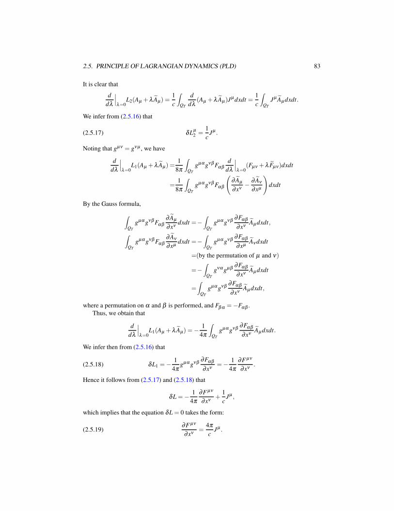
2.5. PRINCIPLE OF LAGRANGIAN DYNAMICS (PLD) 83
It is clear that
d
dλ
∣∣∣λ=0
L2(Aµ +λ Aµ) =1
c
∫
QT
d
dλ(Aµ +λ Aµ)J
µdxdt =1
c
∫
QT
Jµ Aµdxdt.
We infer from (2.5.16) that
(2.5.17) δLµ2 =
1
cJµ .
Noting that gµν = gνµ , we have
d
dλ
∣∣∣λ=0
L1(Aµ +λ Aµ) =1
8π
∫
QT
gµαgνβ Fαβd
dλ
∣∣∣λ=0
(Fµν +λ Fµν)dxdt
=1
8π
∫
QT
gµαgνβ Fαβ
(∂ Aµ
∂xν− ∂ Aν
∂xµ
)dxdt
By the Gauss formula,
∫
QT
gµα gνβ Fαβ∂ Aµ
∂xνdxdt =−
∫
QT
gµα gνβ ∂Fαβ
∂xνAµdxdt,
∫
QT
gµα gνβ Fαβ∂ Aν
∂xµdxdt =−
∫
QT
gµα gνβ ∂Fαβ
∂xµAνdxdt
=(by the permutation of µ and ν)
=−∫
QT
gνα gµβ ∂Fαβ
∂xνAµdxdt
=
∫
QT
gµαgνβ ∂Fαβ
∂xνAµdxdt,
where a permutation on α and β is performed, and Fβ α =−Fαβ .
Thus, we obtain that
d
dλ
∣∣∣λ=0
L1(Aµ +λ Aµ) =− 1
4π
∫
QT
gµαgνβ ∂Fαβ
∂xνAµdxdt.
We infer then from (2.5.16) that
(2.5.18) δL1 =− 1
4πgµα gνβ ∂Fαβ
∂xν=− 1
4π
∂F µν
∂xν.
Hence it follows from (2.5.17) and (2.5.18) that
δL =− 1
4π
∂F µν
∂xν+
1
cJµ ,
which implies that the equation δL = 0 takes the form:
(2.5.19)∂F µν
∂xν=
4π
cJµ .
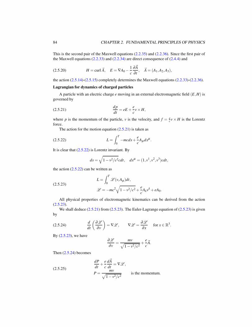
84 CHAPTER 2. FUNDAMENTAL PRINCIPLES OF PHYSICS
This is the second pair of the Maxwell equations (2.2.35) and (2.2.36). Since the first pair of
the Maxwell equations (2.2.33) and (2.2.34) are direct consequence of (2.4.4) and
(2.5.20) H = curl ~A, E = ∇A0 −1
c
∂~A
∂ t, ~A = (A1,A2,A3),
the action (2.5.14)-(2.5.15) completely determines the Maxwell equations (2.2.33)-(2.2.36).
Lagrangian for dynamics of charged particles
A particle with an electric charge e moving in an external electromagnetic field (E,H) is
governed by
(2.5.21)d p
dt= eE +
e
cv×H,
where p is the momentum of the particle, v is the velocity, and f = ecv×H is the Lorentz
force.
The action for the motion equation (2.5.21) is taken as
(2.5.22) L =∫ T
0−mcds+
e
cAµdxµ .
It is clear that (2.5.22) is Lorentz invariant. By
ds =√
1− v2/c2cdt, dxµ = (1,v1,v2,v3)cdt,
the action (2.5.22) can be written as
(2.5.23)L =
∫ T
0L (v,Aµ)dt,
L =−mc2√
1− v2/c2 +e
cAkvk + eA0.
All physical properties of electromagnetic kinematics can be derived from the action
(2.5.23).
We shall deduce (2.5.21) from (2.5.23). The Euler-Lagrange equation of (2.5.23) is given
by
(2.5.24)d
dt
(∂L
∂v
)= ∇L , ∇L =
∂L
∂xfor x ∈ R
3.
By (2.5.23), we have∂L
∂v=
mv√1− v2/c2
+e
c~A.
Then (2.5.24) becomes
(2.5.25)
dP
dt+
e
c
d~A
dt= ∇L ,
P =mv√
1− v2/c2is the momentum.
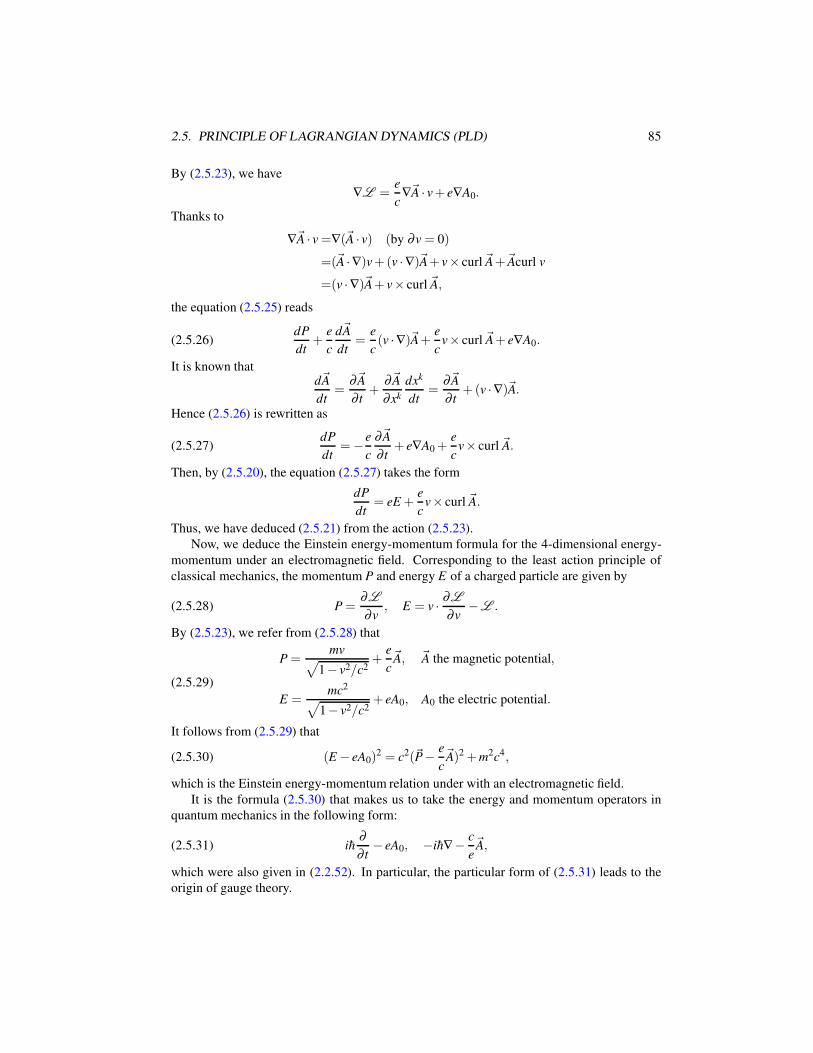
2.5. PRINCIPLE OF LAGRANGIAN DYNAMICS (PLD) 85
By (2.5.23), we have
∇L =e
c∇~A · v+ e∇A0.
Thanks to
∇~A · v =∇(~A · v) (by ∂v = 0)
=(~A ·∇)v+(v ·∇)~A+ v× curl ~A+~Acurl v
=(v ·∇)~A+ v× curl ~A,
the equation (2.5.25) reads
(2.5.26)dP
dt+
e
c
d~A
dt=
e
c(v ·∇)~A+
e
cv× curl ~A+ e∇A0.
It is known thatd~A
dt=
∂~A
∂ t+
∂~A
∂xk
dxk
dt=
∂~A
∂ t+(v ·∇)~A.
Hence (2.5.26) is rewritten as
(2.5.27)dP
dt=−e
c
∂~A
∂ t+ e∇A0 +
e
cv× curl ~A.
Then, by (2.5.20), the equation (2.5.27) takes the form
dP
dt= eE +
e
cv× curl ~A.
Thus, we have deduced (2.5.21) from the action (2.5.23).
Now, we deduce the Einstein energy-momentum formula for the 4-dimensional energy-
momentum under an electromagnetic field. Corresponding to the least action principle of
classical mechanics, the momentum P and energy E of a charged particle are given by
(2.5.28) P =∂L
∂v, E = v · ∂L
∂v−L .
By (2.5.23), we refer from (2.5.28) that
(2.5.29)
P =mv√
1− v2/c2+
e
c~A, ~A the magnetic potential,
E =mc2
√1− v2/c2
+ eA0, A0 the electric potential.
It follows from (2.5.29) that
(2.5.30) (E − eA0)2 = c2(~P− e
c~A)2 +m2c4,
which is the Einstein energy-momentum relation under with an electromagnetic field.
It is the formula (2.5.30) that makes us to take the energy and momentum operators in
quantum mechanics in the following form:
(2.5.31) ih∂
∂ t− eA0, −ih∇− c
e~A,
which were also given in (2.2.52). In particular, the particular form of (2.5.31) leads to the
origin of gauge theory.
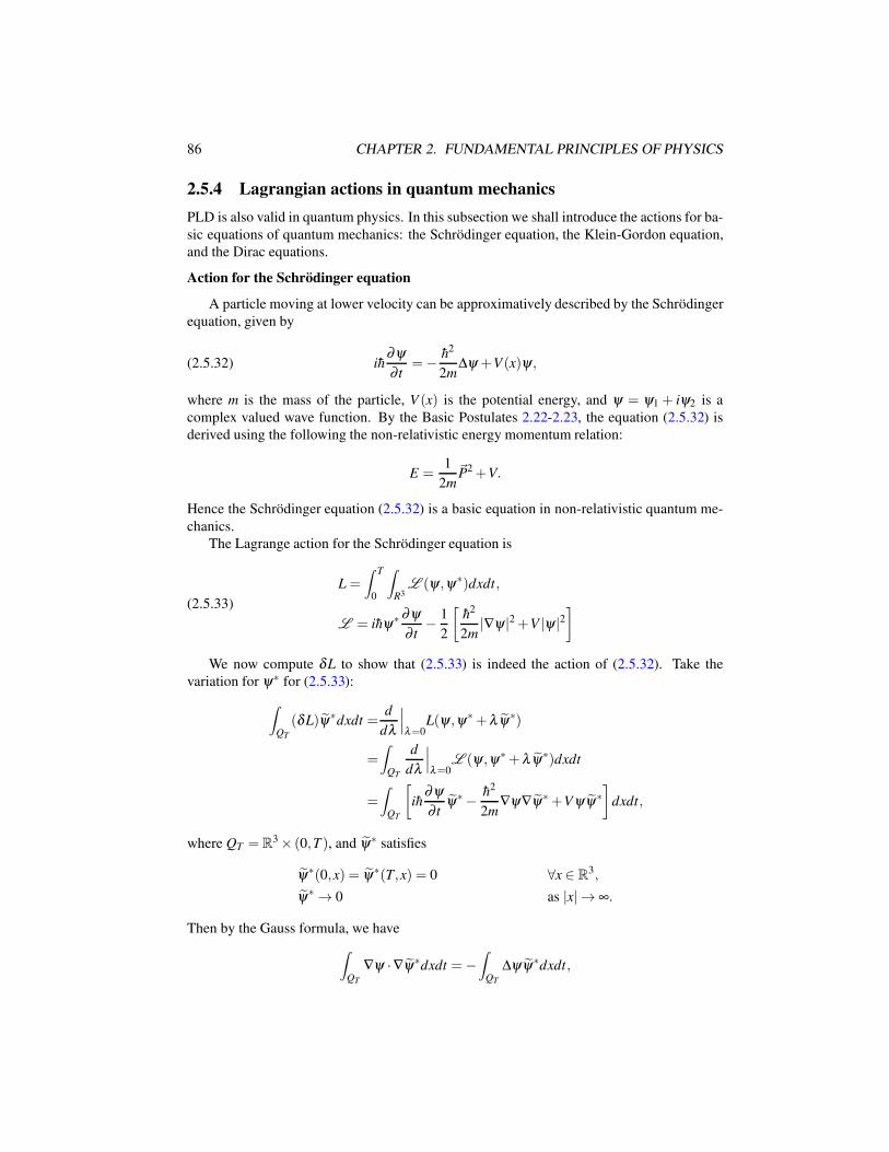
86 CHAPTER 2. FUNDAMENTAL PRINCIPLES OF PHYSICS
2.5.4 Lagrangian actions in quantum mechanics
PLD is also valid in quantum physics. In this subsection we shall introduce the actions for ba-
sic equations of quantum mechanics: the Schrodinger equation, the Klein-Gordon equation,
and the Dirac equations.
Action for the Schrodinger equation
A particle moving at lower velocity can be approximatively described by the Schrodinger
equation, given by
(2.5.32) ih∂ψ
∂ t=− h2
2m∆ψ +V(x)ψ ,
where m is the mass of the particle, V (x) is the potential energy, and ψ = ψ1 + iψ2 is a
complex valued wave function. By the Basic Postulates 2.22-2.23, the equation (2.5.32) is
derived using the following the non-relativistic energy momentum relation:
E =1
2m~P2 +V.
Hence the Schrodinger equation (2.5.32) is a basic equation in non-relativistic quantum me-
chanics.
The Lagrange action for the Schrodinger equation is
(2.5.33)
L =
∫ T
0
∫
R3L (ψ ,ψ∗)dxdt,
L = ihψ∗ ∂ψ
∂ t− 1
2
[h2
2m|∇ψ |2 +V |ψ |2
]
We now compute δL to show that (2.5.33) is indeed the action of (2.5.32). Take the
variation for ψ∗ for (2.5.33):
∫
QT
(δL)ψ∗dxdt =d
dλ
∣∣∣λ=0
L(ψ ,ψ∗+λ ψ∗)
=
∫
QT
d
dλ
∣∣∣λ=0
L (ψ ,ψ∗+λ ψ∗)dxdt
=
∫
QT
[ih
∂ψ
∂ tψ∗− h2
2m∇ψ∇ψ∗+Vψψ∗
]dxdt,
where QT =R3 × (0,T ), and ψ∗ satisfies
ψ∗(0,x) = ψ∗(T,x) = 0 ∀x ∈ R3,
ψ∗ → 0 as |x| → ∞.
Then by the Gauss formula, we have
∫
QT
∇ψ ·∇ψ∗dxdt =−∫
QT
∆ψψ∗dxdt,
2.5. PRINCIPLE OF LAGRANGIAN DYNAMICS (PLD) 87
which implies that
∫
QT
δLψ∗dxdt =
∫
QT
[ih
∂ψ
∂ t+
h2
2m∆ψ −Vψ
]ψ∗dxdt.
Since ψ∗ is arbitrary, we derive that
δL = ih∂ψ
∂ t+
h2
2m∆ψ −Vψ .
Hence we have
(2.5.34)δL
δψ∗ = 0 ⇔ ih∂ψ
∂ t=− h2
2m∆ψ +V(x)ψ .
We can derive in the same fashion that
(2.5.35)δL
δψ= 0 ⇔ −ih
∂ψ∗
∂ t=− h2
2m∆ψ∗+V(x)ψ∗.
It follows from (2.5.34) and (2.5.35) that
δL
δψ∗ =
(δL
δψ
)∗.
In other words, (2.5.34) and (2.5.35) are equivalent, and are exactly the Schrodinger equation.
Action for Klein-Gordon fields
The field equations governing the spin-0 bosons are the Klein-Gordon equations:
(2.5.36)1
c2
∂ 2ψ
∂ t2−∆ψ +
(mc
h
)2
ψ = 0.
It is easy to introduce the Lagrange action for (2.5.36):
(2.5.37) L =
∫
M 4
[∇µψ∇µψ∗+
(mc
h
)2
|ψ |2]√−gdx,
where ∇µ and ∇µ are 4-dimensional gradient operators as defined by (2.2.19), M 4 is the
Minkowski space, and g = det(gµν ).It is readily to see that
δL
δψ∗ =
(δL
δψ
)∗= 0 ⇔ 1
c2
∂ 2ψ
∂ t2−∆ψ +
(mc
h
)2
ψ = 0.
Hence, the Klein-Gordon equation is a variational equation of the action (2.5.37).
Action for Dirac spinor fields
To introduce an action for the Dirac equations introduced in Subsections 2.2.5 and 2.2.6,
we first recall the Dirac equations:
(2.5.38) iγµ ∂ψ
∂xµ− mc
hψ = 0,
88 CHAPTER 2. FUNDAMENTAL PRINCIPLES OF PHYSICS
where ψ = (ψ1,ψ2,ψ3,ψ4)T is the Dirac spinor, and γµ = (γ0,γ1,γ2,γ3) is the Dirac matri-
ces, defined by
(2.5.39) γ0 =
(I 0
0 −I
), γk =
(0 σk
−σk 0
)for k = 1,2,3,
where the Pauli matrices are given by
σ1 =
(0 1
1 0
), σ2 =
(0 −i
i 0
), σ3 =
(1 0
0 −1
).
The Lagrange action of (2.5.38) is
(2.5.40) L =
∫
M 4ψ(iγµ ∂µ −
mc
h)ψ
√−gdx,
where ψ = ψ†γ0.
The Lagrange density of (2.5.40) is
L = ψ(
iγµ∂µ − mc
h
)ψ
is Lorentz invariant. To see this, recall the spinor transformation defined by (2.2.63):
xµ = Lµν xν ⇒ ψ = Rψ ,
which satisfies that (2.2.62):
(2.5.41) (iγµ ∂µ −mc
h)ψ = R(iγµ∂µ − mc
h)ψ ,
where ∂µ = ∂/∂ xµ ,R is as in (2.2.67). By (2.2.68) and
(2.5.42) R†γ0 = γ0R†, (γ0)† = γ0.
It follows from (2.5.41) and (2.4.2) that
ψ(iγµ ∂µ −mc
h)ψ =ψ†R†γ0R
(iγµ∂µ − mc
h
)ψ
=(by ψ†γ0 = ψ)
=ψ(iγµ ∂µ −mc
h)ψ .
It implies that the Lagrange action (2.5.40) is Lorentz invariant.
It is easy to see that
δL
δψ∗ = 0 ⇔ (iγµ ∂µ −mc
h)ψ = 0.
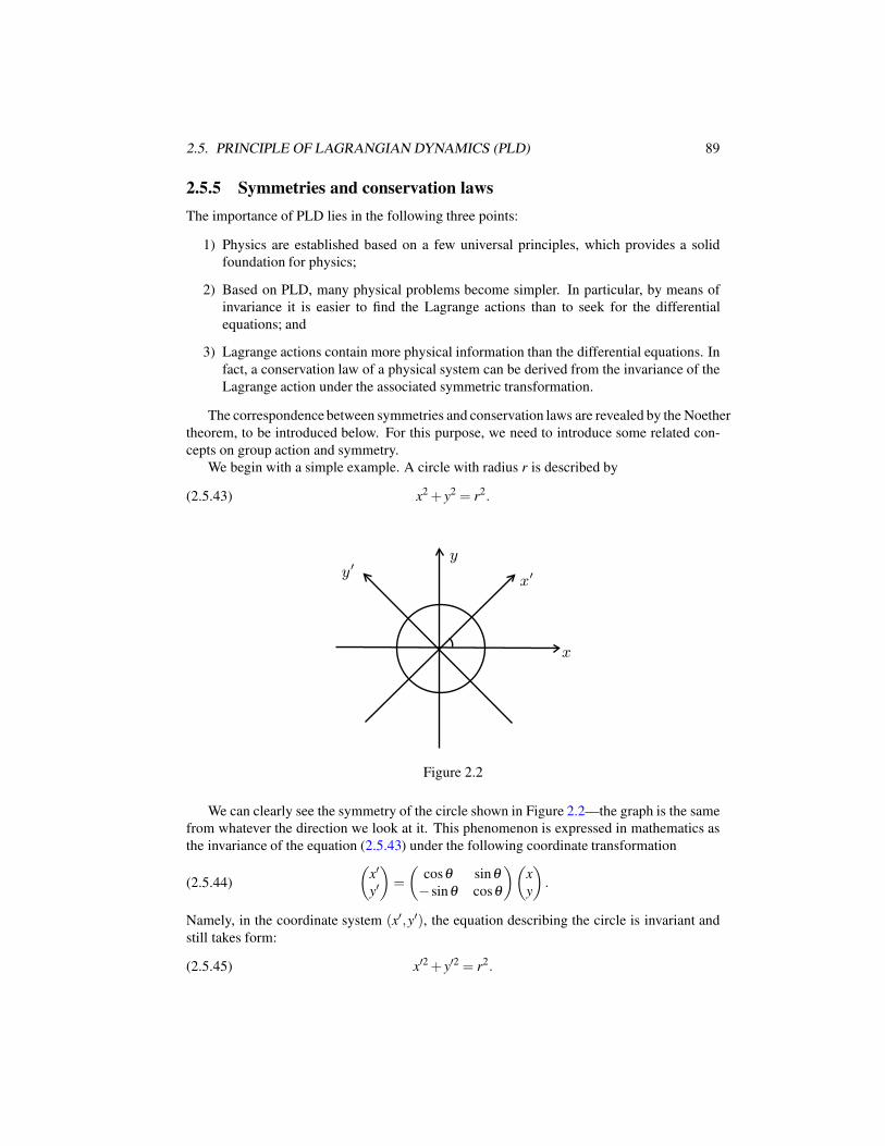
2.5. PRINCIPLE OF LAGRANGIAN DYNAMICS (PLD) 89
2.5.5 Symmetries and conservation laws
The importance of PLD lies in the following three points:
1) Physics are established based on a few universal principles, which provides a solid
foundation for physics;
2) Based on PLD, many physical problems become simpler. In particular, by means of
invariance it is easier to find the Lagrange actions than to seek for the differential
equations; and
3) Lagrange actions contain more physical information than the differential equations. In
fact, a conservation law of a physical system can be derived from the invariance of the
Lagrange action under the associated symmetric transformation.
The correspondence between symmetries and conservation laws are revealed by the Noether
theorem, to be introduced below. For this purpose, we need to introduce some related con-
cepts on group action and symmetry.
We begin with a simple example. A circle with radius r is described by
(2.5.43) x2 + y2 = r2.
x
y
x′y′
Figure 2.2
We can clearly see the symmetry of the circle shown in Figure 2.2—the graph is the same
from whatever the direction we look at it. This phenomenon is expressed in mathematics as
the invariance of the equation (2.5.43) under the following coordinate transformation
(2.5.44)
(x′
y′
)=
(cosθ sinθ−sinθ cosθ
)(x
y
).
Namely, in the coordinate system (x′,y′), the equation describing the circle is invariant and
still takes form:
(2.5.45) x′2 + y′2 = r2.
90 CHAPTER 2. FUNDAMENTAL PRINCIPLES OF PHYSICS
Now, we discuss the symmetry from the viewpoint of action functional and group action.
The key feature is then characterized by the Noether theorem. Let F : R2 →R1 be a function
(a finite dimensional functional) defined by
(2.5.46) F(u) = x2 + y2 for u = (x,y) ∈ R2.
All the transformation matrices in (2.5.44) constitute a group, denoted by SO(2), called the
orthogonal group:
(2.5.47) SO(2) =
Aθ | Aθ =
(cosθ sinθ−sinθ cosθ
), θ ∈R
1
.
The symmetry here is the invariance of the function (2.5.46) under the SO(2) group action:
F(Aθ u) = F(u) ∀Aθ ∈ SO(2).
The generalization to the Lagrangian dynamics is what we shall introduce in this subsection.
Definition 2.37. Let G be a group, X be a Banach space, and F : X → R1 a continuous
functional. Let G be a group acting on X:
(2.5.48)Au ∈ X ∀u ∈ X and A ∈ G,
A(Bu) = (AB)u ∀u ∈ X , A,B ∈ G.
The functional F is called invariant under the action (2.5.48) of G, if
F(Au) = F(u) ∀A ∈ G.
We consider a Lagrange action defined on a function space X :
(2.5.49) L(u, u) =
∫ T
0L (u, u)dt for u ∈ X ,
where the Lagrange density L is defined by
L (u, u) =
L (x, x) for an N-body system,∫
Ωg(u, u,Du, · · · ,Dmu)dx otherwise.
The following theorem is the well-known Noether theorem, which provides a correspon-
dence between symmetries and conservation laws in the Lagrangian system (2.5.49).
Theorem 2.38 (Noether Theorem). Let G = Aλ | λ ∈ R1 be a parameterized group, and
L(u, u) be the Lagrange action given by (2.5.49). If L is invariant under the group action of
G:
(2.5.50) L (u, u) = L (Aλ u,Aλ u) ∀Aλ ∈ G,
then the system has a conserved quantity induced by G, expressed as
(2.5.51) I(u, u) =⟨δL
δ u,
dAλ (u)
dλ
∣∣∣λ=0
⟩for Aλ ∈ G.
In other words,
(2.5.52)d
dtI(u, u) = 0 for any solutions u of δL = 0.
2.5. PRINCIPLE OF LAGRANGIAN DYNAMICS (PLD) 91
Remark 2.39. The correspondence between symmetries and conservation laws in the Noether
Theorem holds true as well for discrete transformation groups, such as the reflections of time
and space.
Proof of Theorem 2.38. Let (u,ut) be a solution of the variational equation of L given by
(2.5.49):
(2.5.53)d
dt
(δL (u, u)
δ u
)=
δ
δuL (u, u).
By the invariance (2.5.50), (Aλ u,Aλ u) are also solutions of (2.5.53). Then it follows from
(2.5.50) that
(2.5.54) 0 =∂L (Aλ u,Aλ u)
∂λ=⟨δL
∂Φ,
dΦ
dλ
⟩+⟨δL
δ Φ,
dΦ
dλ
⟩,
where Φ = Aλ u. Since (Aλ u,Aλ u) satisfies (2.5.53), we have
(2.5.55)δ
δΦL (Aλ u,Aλ u) =
d
dt
(δL (Aλ u,Aλ u)
δ Φ
).
Inserting (2.5.55) in (2.5.54) we deduce that for any Φ = Aλ u and any λ ∈ R1,
0 =⟨ d
dt
(δL
δ Φ
),
dΦ
dλ
⟩+⟨∂L
∂ Φ,
d
dt
(dΦ
dλ
)⟩=
d
dt
⟨δL
δ Φ,
dΦ
dλ
⟩,
which implies thatd
dtI(u, u) =
d
dt
⟨δL
δ Φ,
dΦ
dλ
⟩∣∣∣λ=0
= 0,
where Aλ u = u if λ = 0. The proof is complete.
We now give two examples to show how to apply the Noether theorem to a specific
physical problem.
Example 2.40. Consider an N-body motion, such as a system of N planets. Let mk and xk be
the mass and the coordinates of the k-th body. The Lagrange density is
(2.5.56) L =1
2
N
∑k=1
mk|xk|2 −∑i6= j
V (|xi − x j|).
Note that x is the u in Theorem 2.38. Let G be the translation group:
G = Aλ | Aλ : R3 →R
3, Aλ x = x+λ~r,
where~r is a given vector. It clear that (2.5.56) is invariant under the transformation of G. By
δL
δ x=
(∂L
∂ x1
, · · · , ∂L
∂ xN
)= (m1x1, · · · ,mN xN),
d
dλ
∣∣∣λ=0
Aλ x =d
dλ
∣∣∣λ=0
(x+λ~r) = (~r, · · · ,~r︸ ︷︷ ︸N
).
92 CHAPTER 2. FUNDAMENTAL PRINCIPLES OF PHYSICS
Hence we derive from the Noether Theorem that
I =⟨δL
δ x,
d
dλ
∣∣∣λ=0
Aλ x⟩=
N
∑k=1
mk〈xk,~r〉
is conserved, and is the total momentum in the direction ~r. Thus we have shown that the
translation invariance corresponds to momentum conservation.
Example 2.41. Consider the Schrodinger equation, the action is given by (2.5.33), and
(2.5.57) L (ψ , ψ) =
∫
R3
[−ihψ∗ψ +
1
2
(h2
2m|∇ψ |2 +V |ψ |2
)]dx.
Let G be the phase rotation group
G = Aλ = eiλ | λ ∈ R1.
It is clear that (2.5.57) is invariant under the phase rotation:
ψ → Aλ ψ = eiλ ψ .
We see thatδL
δψ=−ihψ∗,
d
dλAλ ψ |λ=0 = iψ .
Thus, the quantity (2.5.51) reads as
I(ψ , ψ) =⟨δL
δψ,
d
dλAλ ψ
⟩=∫
R3h|ψ |2dx.
Hence, the modulus of ψ
(2.5.58)
∫
R3|ψ |2dx is conserved.
The property (2.5.58) is just what we need because in quantum mechanics, we have
(2.5.59)
∫
R3|ψ |2dx = 1.
Here, the conservation (2.5.59) corresponds to the invariance of phase rotation of the wave
function ψ .
Remark 2.42. In classical mechanics, the energy conservation can be deduced from the time
translation invariance
(2.5.60) t → t +λ for λ ∈R1.
However, instead of the formula (2.5.51), it is derived using following relation:
(2.5.61) dH =∂H
∂ pd p+
∂H
∂qdq− ∂L
∂ tdt,
2.6. PRINCIPLE OF HAMILTONIAN DYNAMICS (PHD) 93
where H = H(q, p, t) is the total energy, L is the Lagrangian, and q, p satisfy the Hamilton
equations
(2.5.62)dq
dt=
∂H
∂ p,
d p
dt=−∂H
∂q.
If L = L (q, q, t) is invariant under the translation (2.5.60), then L does not explicitly con-
tain time t, i.e.∂L
∂ t= 0.
Then it follows from (2.5.61) and (2.5.62) that
dH
dt=−∂L
∂ t= 0.
Hence the energy conservation is deduced using the time translation invariance.
We end this section with some relations of symmetries and conservation laws:
energy ⇔ time translation,
momentum ⇔ space translation,
angular Momentum ⇔ space rotation,
particle number ⇔ phase rotation,
parity ⇔ space reflection.
2.6 Principle of Hamiltonian Dynamics (PHD)
2.6.1 Hamiltonian systems in classical mechanics
In classical mechanics, the principle of Hamiltonian dynamics (PHD) consists of the follow-
ing three main ingredients:
1) for an isolated (conserved) mechanical system, its states are described by a set of state
variables given by
(2.6.1) q1, · · · ,qN , p1, · · · , pN ;
2) its total energy H is a function of (2.6.1), i.e.
(2.6.2) H = H(q, p),
3) the state variables q and p satisfy
(2.6.3)
dqk
dt=
∂H
∂ pk
,
d pk
dt=− ∂H
∂qk
for 1 ≤ k ≤ N.
94 CHAPTER 2. FUNDAMENTAL PRINCIPLES OF PHYSICS
The state variables qk (1 ≤ k ≤ N) represent positions, and pk (1 ≤ k ≤ N) represent momen-
tums. The system (2.6.1)-(2.6.3) is called Hamiltonian system.
In physics, PLD and PHD are two independent fundamental principles. However, the two
sets of equations derived from PLD and PHD are usually equivalent.
In classical mechanics, Hamiltonian systems and Lagrange systems can be transformed
to each other by the Legendre transformation. We start with a simple example. Consider a
particle with mass m in a force field F . The Lagrange action for this system is given by
(2.6.4)
L =
∫ T
0L (q, q)dt,
L = T −V =1
2mq2 −Fq,
where q stands for position, and the Euler-Lagrange equation of (2.6.4) is the Newtonian
Second Law, written as
(2.6.5)d
dt
δL
δ q=
δL
δq⇒ mq = F.
Based on (2.6.1)-(2.6.3), the state variables q, p of PHD are
(2.6.6) q as in (2.6.4) and p = mq.
The total energy is
(2.6.7) H =1
2mp2 +Fq,
and the Hamilton equations of (2.6.7) are given by
(2.6.8)
d p
dt=
∂H
∂q= F,
dq
dt=−∂H
∂ p=
1
mp.
By (2.6.6), it is clear that
(2.6.9) Hamilton Eqs (2.6.8) = Lagrange Eq (2.6.5) = Newton 2nd Law.
The equivalences in (2.6.9) only manifest that the three principles have an intrinsic relation.
In particular, by (2.6.4)-(2.6.7), the variables q, q of PLD and the variables q, p of PHD have
the relation:
(2.6.10) p =δL
δ q(by
δL
δ q=
∂L
∂ q= mq),
and the Lagrange density L (q, q) and the Hamilton energy H(q, p) are related by
(2.6.11) pq−L (q, q) = H(q, p).
2.6. PRINCIPLE OF HAMILTONIAN DYNAMICS (PHD) 95
In this example, the two relations (2.6.10) and (2.6.11) are obtained directly by their
physical meanings, and by which we can deduce one by another.
In fact, the relations (2.6.10) and (2.6.11) are also valid in general.We discuss this problem
as follows.
Consider a mechanical system. For PLD, the state variables are positions qk and velocities
qk:
(2.6.12) q1, · · · ,qN and q1, · · · , qN ,
The Lagrange action is given by
(2.6.13) L =
∫ T
0L (q, q)dt.
For PHD, the state variables are:
(2.6.14) q1, · · · ,qN and p1, · · · , pN ,
The Hamilton energy is:
(2.6.15) H = H(q, p).
The two systems (2.6.12)-(2.6.13) and (2.6.14)-(2.6.15) of PLD and PHD satisfy the fol-
lowing relations, which implies the equivalence of PLD and PHD in classical mechanics.
Dynamical Relation 2.43 (PLD and PHD). For the two systems of PLD and PHD in classical
mechanics, the following conclusions hold true:
1) The two sets (2.6.12) and (2.6.14) of variables satisfy the following relation:
(2.6.16) pk =∂L (q, q)
∂ qk
for 1 ≤ k ≤ N.
2) The two functions (2.6.13) and (2.6.15) satisfy the following relation, which is usually
called the Legendre transformation:
(2.6.17) pkqk −L (q, q) = H(q, p).
By (2.6.16)-(2.6.17), if we have obtained the PLD system (2.6.12)-(2.6.13), then by the
implicit function theorem we can solve from (2.6.16) the functions
(2.6.18) qk = fk(q, p).
Then, inserting (2.6.18) in the left-hand side of (2.6.17) we deduce the expression of the
Hamilton energy:
(2.6.19) H(q, p) = pk fk(q, p)−L (q, f (q, p)),
which gives rise to the Hamiltonian system (2.6.3). In other words, we can derive the Hamil-
tonian dynamics from the Lagrangian dynamics by the relations (2.6.16) and (2.6.17).
96 CHAPTER 2. FUNDAMENTAL PRINCIPLES OF PHYSICS
Conversely, if we know the PHD system (2.6.14) and (2.6.15), then it follows from
(2.6.16) and (2.6.17) that the Lagrange density L satisfies
(2.6.20) H
(x,
∂L
∂y
)− yk
∂L
∂yk
+L (x,y) = 0.
Theoretically we can solve the differential equation (2.6.20), and obtain the solution L =L (x,y). Let x = q and y = q, then we deduce the expression for the Lagrange density from
the Hamilton function H(q, p).
Remark 2.44. We remark that both PLD and PHD are independent to each other. However,
the PLD dynamical system (2.1.5)-(2.1.8) and the PHD dynamical system (2.6.1)-(2.6.3) are
equivalent in mechanics by (2.6.16) and (2.6.17). But we shall see later that the relations
(2.6.16) and (2.6.17) are not valid in electromagnetism where PLD and PHD still hold true.
In addition, the differential dH is given by
(2.6.21) dH =∂H
∂qk
dqk +∂H
∂ pk
d pk +∂H
∂ tdt.
By (2.6.17),
(2.6.22) dH = qkd pk −∂L
∂qk
dqk −∂L
∂ tdt.
It follows from (2.6.21) and (2.6.22) that
qk =∂H
∂ pk
,(2.6.23)
∂H
∂qk
=−∂L
∂qk
,(2.6.24)
∂H
∂ t=−∂L
∂ t.(2.6.25)
From (2.6.21) and (2.6.25) we deduce (2.5.61). Then by (2.6.16) and the Lagrange equation
(2.1.8), we haved pk
dt=
d
dt
(δL
δ qk
)=
∂L
∂qk
.
Hence (2.6.24) becomes
(2.6.26) pk =− ∂H
∂qk
.
Thus, by the relations (2.6.16) and (2.6.17) we deduce the equivalence of PLD dynamics and
PHD dynamics in another fashion.
2.6.2 Dynamics of conservative systems
Energy conservation is a universal law in physics. It implies that the PHD is a universal
principle to describe conservative physical systems. In other words, the Hamilton principle
2.6. PRINCIPLE OF HAMILTONIAN DYNAMICS (PHD) 97
introduced in the last subsection can be generalized to all physical fields. The most remark-
able characteristic of PHD is that the total energy H of the physical system is conserved:
(2.6.27)d
dtH(q(t), p(t)) = 0,
where (q, p) are the solutions of the Hamiltonian system.
Now, we introduce the PHD.
Principle 2.45 (Hamiltonian Dynamics). For any conservative physical system, there are two
sets of state functions
(2.6.28) u = (u1, · · · ,uN) and v = (v1, · · · ,vN),
such that the energy density H is a function of (2.6.28):
(2.6.29) H = H (u,v, · · · ,Dmu,Dmv), m ≥ 0.
The total energy of the system is
(2.6.30) H =
∫
ΩH (u,v, · · · ,Dmu,Dmv)dx, Ω ⊂ R
3,
provided that the system is described by continuous fields. Moreover the state functions u and
v satisfy the equations
(2.6.31)
∂u
∂ t= α
δH
δv,
∂v
∂ t=−α
δH
δu,
where α is a constant.
In general, the energy density (2.6.29) for a continuous field system depends on u,v only
up to the first-order derivatives Du and Dv:
(2.6.32) H = H (u,v,Du,Dv).
Then the Hamilton equations (2.6.31) can be expressed in the following form:
(2.6.33)
∂uk
∂ t= α
[−∂ j
(∂H
∂ζ jk
)+
∂H
∂vk
],
∂vk
∂ t= α
[∂ j
(∂H
∂ξ jk
)− ∂H
∂uk
],
where ξ jk,ζ jk are variables corresponding to ∂ juk and ∂ jvk.
Hereafter, we always assume that H is in the form (2.6.32). The following theorem
shows that the total energy H of the Hamiltonian system (2.6.31) (or (2.6.33)) is conserved.
98 CHAPTER 2. FUNDAMENTAL PRINCIPLES OF PHYSICS
Theorem 2.46 (Energy Conservation). Let (u,v) be the solutions of (2.6.33), and H does not
explicitly contain time t. Then the energy H(u,v) is conserved, i.e. H(u,v) satisfies (2.6.27)
with q = u and p = v, if Ω = R3. In addition, if Ω 6= R
3, then we have
(2.6.34)dH
dt=
∫
∂Ω
[∂H
∂ξi j
∂u j
∂ t+
∂H
∂ζi j
∂v j
∂ t
]nids,
where n = (n1,n2,n3) is the unit outward normal at ∂Ω.
Proof. For (2.6.32), we have
(2.6.35)dH
dt=
∫
Ω
[∂H
∂uk
∂uk
∂ t+
∂H
∂ξi j
∂i
(∂u j
∂ t
)+
∂H
∂vk
∂vk
∂ t+
∂H
∂ζi j
∂i
(∂v j
∂ t
)]dx.
By the Gauss formula,
∫
Ω
∂H
∂ξi j
∂i
(∂u j
∂ t
)dx =
∫
∂Ω
∂H
∂ξi j
∂u j
∂ tnids−
∫
Ω∂i
(∂H
∂ξi j
)∂u j
∂ tdx,
∂H
∂ζi j
∂i
(∂v j
∂ t
)dx =
∫
∂Ω
∂H
∂ζi j
∂v j
∂ tnids−
∫
Ω∂i
(∂H
∂ζi j
)∂v j
∂ tdx.
Hence (2.6.35) is rewritten as
d
dtH =
∫
Ω
[(∂H
∂uk
− ∂i
(∂H
∂ξik
))∂uk
∂ t+
(∂H
∂vk
− ∂i
(∂H
∂ζik
))∂vk
∂ t
]dx(2.6.36)
+
∫
∂Ω
[∂H
∂ξi j
∂u j
∂ t+
∂H
∂ζi j
∂v j
∂ t
]nids.
Since (u,v) is a solution of (2.6.33), then (2.6.36) becomes
dH
dt=
∫
∂Ω
[∂H
∂ξi j
∂u j
∂ t+
∂H
∂ζi j
∂v j
∂ t
]nids,
and (2.6.34) follows.
If Ω = R3 (i.e. ∂Ω = /0) or u = v = 0 on ∂Ω, then
d
dtH(u,v) = 0 for (u,v) satisfy (2.6.33).
The proof is complete.
Remark 2.47. The integral functions in (2.6.34):
(2.6.37)
P = (P1,P2,P3),
Pk =−[
∂H
∂ξk j
∂u j
∂ t+
∂H
∂ζk j
∂v j
∂ t
],
are the energy fluxes. Hence (2.6.34) can be expressed as
d
dtH(u,v) =−
∫
∂ΩP ·nds,
2.6. PRINCIPLE OF HAMILTONIAN DYNAMICS (PHD) 99
which means that the rate of energy change in Ω equals to the difference of the input and
output of energy flow crossing the boundary of Ω per unit time. Consequently (2.6.34) is
equivalent to energy conservation.
In the Lagrangian dynamics, Noether Theorem 2.38 gives a correspondence between
symmetries and conservations, and provides a way to seek the conservation laws. Likewise,
the Hamiltonian dynamics provides another criterion to find conservation laws.
Let S(u,v) be a functional given by
(2.6.38) S(u,v) =
∫
ΩS(u,v,Du,Dv)dx.
The following theorem provides a condition for S(u,v) to be a conserved quantity.
Theorem 2.48 (Conservation Laws of Hamiltonian System). Let S(u,v) be a functional as
given by (2.6.38). If S and the Hamilton energy H satisfy the following relation
∫
Ω
[∂S
∂uk
− ∂i
(∂S
∂ξik
)][∂H
∂vk
− ∂i
(∂H
∂ζik
)]dx(2.6.39)
=
∫
Ω
[∂S
∂vk
− ∂i
(∂S
∂ζik
)][∂H
∂uk
− ∂i
(∂H
∂ξik
)]dx,
for solutions (u,v) of (2.6.33), then S is a conserved quantity of the Hamiltonian system.
Namely, S satisfies that
(2.6.40)dS
dt=−
∫
∂ΩPs ·nds,
where Ps = (P1s ,P
2s ,P
3s ) is the flux given by
Pks =−
[∂S
∂ξk j
∂u j
∂ t+
∂S
∂ζk j
∂v j
∂ t
].
Proof. The proof is similar to that of Theorem 2.46. By
dS
dt=
∫
Ω
[∂S
∂u j
∂u j
∂ t+
∂S
∂ξi j
∂i
(∂u j
∂ t
)+
∂S
∂v j
∂v j
∂ t+
∂S
∂ζi j
∂i
(∂v j
∂ t
)]dx
=
∫
Ω
[(∂S
∂u j
− ∂i
(∂S
∂ξi j
))∂u j
∂ t+
(∂S
∂v j
− ∂i
(∂S
∂ζi j
))∂v j
∂ t
]dx
+
∫
∂ΩPk
s ·nkdS.
By (2.6.33) and (2.6.39) we deduce (2.6.40). The proof is complete.
In fact, Theorem 2.46 is a special case of Theorem 2.48 for S=H. Theorem 2.48 is useful
for Hamiltonian systems.
100 CHAPTER 2. FUNDAMENTAL PRINCIPLES OF PHYSICS
2.6.3 PHD for Maxwell electromagnetic fields
PHD is also valid in the Maxwell electrodynamics. To establish the Hamiltonian dynamics
for electromagnetism, we first determine the conjugate field functions as follows
(2.6.41)u = E = (E1,E2,E3),v = A = (A1,A2,A3),
where E is the electric field, and A is the magnetic potential. The Hamilton energy H is given
by
(2.6.42)
H =
∫
ΩH (E,A)dx,
H =1
8π(E2 + |curl A|2)+ 1
4π∇ϕ ·E − 1
cJ ·A,
where ϕ is the electric potential, and J is the current. Using
⟨δH
δE, E⟩=
d
dλ
∣∣∣λ=0
H(E +λ E,A),
⟨δH
δA, A⟩=
d
dλ
∣∣∣λ=0
H(E,A+λ A),
we can compute the derivatives of (2.6.42) as follows:
δH
δE=
1
4π(E +∇ϕ),
δH
δA=
1
4πcurl2A− 1
cJ.
Thus, the Hamilton equations (2.6.31) are in the form:
(2.6.43)
1
c
∂E
∂ t= 4π
δH
δA= curl2A− 4π
cJ,
1
c
∂A
∂ t=−4π
δH
δE=−E −∇ϕ ,
which are the classical Maxwell equations (2.2.33) and (2.2.35).
Remark 2.49. We note that the Lagrange action of electromagnetism defined by (2.4.15) can
be expressed as
(2.6.44) LEM =
∫
M 4
[−1
2|curl A|2 + 1
2E2 +
4π
cAµJµ
]dxdt,
where
E =−1
c
∂A
∂ t−∇A0, Aµ = (A0,A1,A2,A3).
The fields of PLD are given by
A0,A1,A2,A3 and A0, A1, A2, A3 (A0 = ϕ),
2.6. PRINCIPLE OF HAMILTONIAN DYNAMICS (PHD) 101
and the fields of PHD are
A1,A2,A3 and E1,E2,E3.
It is clear that1
4πE(−A)− 1
4πLEM = H (A,E)− 1
cϕJ0,
and J0 = ρ . Hence, the relation (2.6.17) does not hold true in general.
Now, we consider the energy conservation. When H contains ∇ϕ and J, which depend
on t, the Hamilton H = H (A,E, t) contains explicitly t. It implies that the Maxwell fields
have energy exchange with other charged particles. Then H is not conserved.
As there is no charged particles in Ω, then
(ρ ,J) = 0 in Ω.
In this case, ∫
Ω∇ϕ ·Edx =−
∫
Ωϕdiv Edx =−
∫
Ω4πϕρdx = 0.
Hence, the Hamilton energy (2.6.42) becomes
(2.6.45) H =1
8π
∫
Ω(E2 + |curl A|2)dx.
By (2.6.37), the energy flux P defined in (2.6.45) reads
P =1
4πcurl A× ∂A
∂ t
Note that∂A
∂ t=−cE, curl A = B (B the magnetic field),
Then, by (2.6.34) we have that
dH
dt=−
∫
∂ΩP ·nds =−
∫
∂Ω
( c
4πE ×B
)·nds.
The field
P =c
4πE ×B
is the Poynting vector, represents the energy flux density of an electromagnetic field.
2.6.4 Quantum Hamiltonian systems
In quantum physics, the state functions are a set of complex valued wave functions:
ψ = (ψ1, · · · ,ψN)T , N ≥ 1,
and ψk are as
(2.6.46) ψk = ψ1k + iψ2
k for 1 ≤ k ≤ N.
102 CHAPTER 2. FUNDAMENTAL PRINCIPLES OF PHYSICS
In view of PHD for a quantum system, the conjugate fields are taken as real and imaginary
parts of the wave functions in (2.6.46):
(2.6.47) ψ11 , · · · ,ψ1
N and ψ21 , · · · ,ψ2
N .
Let H = H(ψ) be the Hamilton energy. Then the Hamilton equations for the quantum system
are as follows:
(2.6.48)
α∂ψ1
k
∂ t=
δ
δψ2k
H,
α∂ψ2
k
∂ t=− δ
δψ1k
H,
for 1 ≤ k ≤ N,
where α is a constant.
We now introduce quantum Hamiltonian systems for the Schrodinger equation, the Weyl
equation, the Dirac equations, the Klein-Gordon equation, and the BEC equation.
1. Schrodinger equation:
(2.6.49) ih∂ψ
∂ t=− h2
2m∆ψ +V(x)ψ ,
where ψ = ψ1 + iψ2. The Hamilton energy of (2.6.49) is given by
H(ψ) =1
2
∫
Ω
[h2
2m|∇ψ |2 +V(x)|ψ |2
]dx.
It is easy to derive that
δ
δψ1H =− h2
2m∆ψ1 +Vψ1,
δ
δψ2H =− h2
2m∆ψ2 +Vψ2.
Hence, the Hamiltonian system is
(2.6.50)
h∂ψ1
∂ t=− h2
2m∆ψ2 +Vψ2,
h∂ψ2
∂ t=
h2
2m∆ψ2 −Vψ2.
It is clear that (2.6.50) and (2.6.49) are equivalent.
2. Weyl equations:
(2.6.51)1
c
∂ψ
∂ t= (~σ ·∇)ψ ,
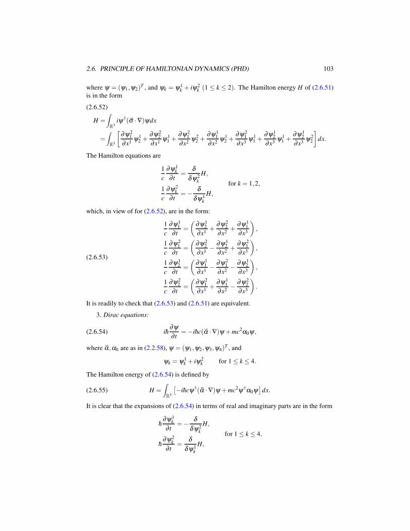
2.6. PRINCIPLE OF HAMILTONIAN DYNAMICS (PHD) 103
where ψ = (ψ1,ψ2)T , and ψk = ψ1
k + iψ2k (1 ≤ k ≤ 2). The Hamilton energy H of (2.6.51)
is in the form
H =∫
R3iψ†(~σ ·∇)ψdx
(2.6.52)
=
∫
R3
[∂ψ2
1
∂x1ψ1
2 +∂ψ2
2
∂x1ψ1
1 +∂ψ2
1
∂x2ψ2
2 +∂ψ1
1
∂x2ψ1
2 +∂ψ2
1
∂x3ψ1
1 +∂ψ1
2
∂x3ψ1
1 +∂ψ1
2
∂x3ψ2
2
]dx.
The Hamilton equations are
1
c
∂ψ1k
∂ t=
δ
δψ2k
H,
1
c
∂ψ2k
∂ t=− δ
δψ1k
H,
for k = 1,2,
which, in view of for (2.6.52), are in the form:
(2.6.53)
1
c
∂ψ11
∂ t=
(∂ψ1
2
∂x1+
∂ψ22
∂x2+
∂ψ11
∂x3
),
1
c
∂ψ21
∂ t=
(∂ψ2
2
∂x1− ∂ψ1
2
∂x2+
∂ψ21
∂x3
),
1
c
∂ψ12
∂ t=
(∂ψ1
1
∂x1− ∂ψ2
1
∂x2− ∂ψ1
2
∂x3
),
1
c
∂ψ22
∂ t=
(∂ψ2
1
∂x1+
∂ψ11
∂x2− ∂ψ2
2
∂x3
).
It is readily to check that (2.6.53) and (2.6.51) are equivalent.
3. Dirac equations:
(2.6.54) ih∂ψ
∂ t=−ihc(~α ·∇)ψ +mc2α0ψ ,
where ~α,α0 are as in (2.2.58), ψ = (ψ1,ψ2,ψ3,ψ4)T , and
ψk = ψ1k + iψ2
k for 1 ≤ k ≤ 4.
The Hamilton energy of (2.6.54) is defined by
(2.6.55) H =∫
R3
[−ihcψ†(~α ·∇)ψ +mc2ψ†α0ψ
]dx.
It is clear that the expansions of (2.6.54) in terms of real and imaginary parts are in the form
h∂ψ1
k
∂ t=− δ
δψ2k
H,
h∂ψ2
k
∂ t=
δ
δψ1k
H,
for 1 ≤ k ≤ 4,
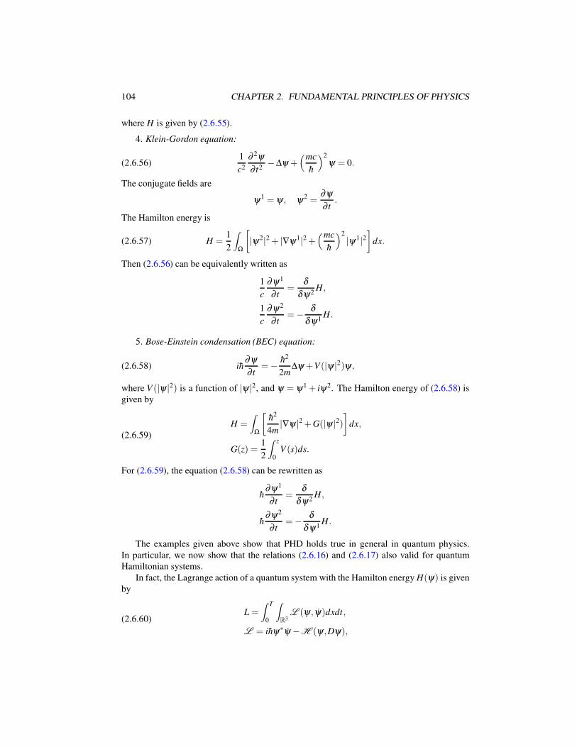
104 CHAPTER 2. FUNDAMENTAL PRINCIPLES OF PHYSICS
where H is given by (2.6.55).
4. Klein-Gordon equation:
(2.6.56)1
c2
∂ 2ψ
∂ t2−∆ψ +
(mc
h
)2
ψ = 0.
The conjugate fields are
ψ1 = ψ , ψ2 =∂ψ
∂ t.
The Hamilton energy is
(2.6.57) H =1
2
∫
Ω
[|ψ2|2 + |∇ψ1|2 +
(mc
h
)2
|ψ1|2]
dx.
Then (2.6.56) can be equivalently written as
1
c
∂ψ1
∂ t=
δ
δψ2H,
1
c
∂ψ2
∂ t=− δ
δψ1H.
5. Bose-Einstein condensation (BEC) equation:
(2.6.58) ih∂ψ
∂ t=− h2
2m∆ψ +V(|ψ |2)ψ ,
where V (|ψ |2) is a function of |ψ |2, and ψ = ψ1 + iψ2. The Hamilton energy of (2.6.58) is
given by
(2.6.59)
H =
∫
Ω
[h2
4m|∇ψ |2 +G(|ψ |2)
]dx,
G(z) =1
2
∫ z
0V (s)ds.
For (2.6.59), the equation (2.6.58) can be rewritten as
h∂ψ1
∂ t=
δ
δψ2H,
h∂ψ2
∂ t=− δ
δψ1H.
The examples given above show that PHD holds true in general in quantum physics.
In particular, we now show that the relations (2.6.16) and (2.6.17) also valid for quantum
Hamiltonian systems.
In fact, the Lagrange action of a quantum system with the Hamilton energy H(ψ) is given
by
(2.6.60)L =
∫ T
0
∫
R3L (ψ , ψ)dxdt,
L = ihψ∗ψ −H (ψ ,Dψ),
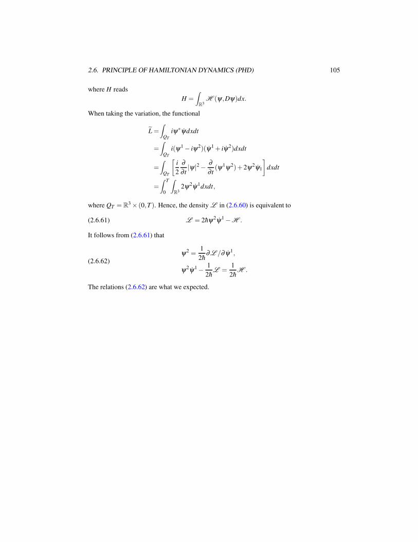
2.6. PRINCIPLE OF HAMILTONIAN DYNAMICS (PHD) 105
where H reads
H =∫
R3H (ψ ,Dψ)dx.
When taking the variation, the functional
L =
∫
QT
iψ∗ψdxdt
=
∫
QT
i(ψ1 − iψ2)(ψ1 + iψ2)dxdt
=
∫
QT
[i
2
∂
∂ t|ψ |2 − ∂
∂ t(ψ1ψ2)+ 2ψ2ψ1
]dxdt
=
∫ T
0
∫
R32ψ2ψ1dxdt,
where QT =R3 × (0,T ). Hence, the density L in (2.6.60) is equivalent to
(2.6.61) L = 2hψ2ψ1 −H .
It follows from (2.6.61) that
(2.6.62)
ψ2 =1
2h∂L /∂ψ1,
ψ2ψ1 − 1
2hL =
1
2hH .
The relations (2.6.62) are what we expected.

106 CHAPTER 2. FUNDAMENTAL PRINCIPLES OF PHYSICS
Chapter 3
Mathematical Foundations
The aim of this chapter is to provide mathematical foundations for the remaining part of
the book on the unified field theory, elementary particles, quantum physics, astrophysics and
cosmology.
As addressed in Chapter 2, Nature speaks the language of mathematics. Thanks to Ein-
stein’s principle of equivalence and the geometric interaction mechanism, the space-time
is a 4D Riemannian manifold M , and physical fields are regarded as functions on vec-
tor bundles over the base manifold M . For example, the Riemannian metric gµν , rep-
resenting the gravitational potential, is a function on the second-order cotangent bundle,
gµν : M → T ∗M ⊗ T ∗M ; the electromagnetic field Aµ is a function on the cotangent
bundle Aµ : M → T ∗M ; the SU(2) gauge fields for the weak interaction is a function
W aµ : M → (T ∗M )3; and the SU(3) gauge fields for the strong interaction is a function
Skµ : M → (T ∗M )8. Also, the Dirac spinor field is defined a complex bundle: Ψ : M →
M ⊗p C4.
The three most fundamental symmetries of Nature are the principle of Lorentz invariance,
the principle of general relativity, and the principle of gauge invariance. They lead to trans-
formations in either the base space-time manifold M , or the corresponding vector bundles.
In summary, we have the following
1) The space-time is a 4D Riemannian manifold, and all physical fields are
functions on vector bundles over the space-time manifold M ⊗p EN; and
2) Fundamental symmetries are invariances of physical field equations under
the underlying transformations on the corresponding vector bundles.
The basic concepts in Section 3.1 include Riemannian manifolds such as the space-time
manifold, vector bundles, tensor fields, connections and linear transformations on vector bun-
dles. It is particularly important that we identify all physical fields as functions on proper
vector bundles defined on the space-time manifold, and symmetries correspond then to linear
transformations on the corresponding vector bundles.
Section 3.2 is on basic functional analysis and partial differential equations on manifolds,
which are needed for rigorous proofs of theorems and concepts used in later chapters of the
book. The readers may consult other references such as (Ma, 2011).
107
108 CHAPTER 3. MATHEMATICAL FOUNDATIONS
Section 3.3 proves the orthogonal decomposition theorem for tensors on Riemannian
manifolds, which forms the mathematical foundation for the principle of interaction dynamics
(PID), postulated by (Ma and Wang, 2014e, 2015a). Basically, PID takes the variation of the
Lagrangian action L(u) under the generalized energy-momentum conservation constraints,
which we call divA-free constraints with A being the gauge potentials:
(3.0.1) 〈δL(u0),X〉= d
dλ
∣∣∣λ=0
L(u0 +λ X) = 0 ∀ divAXdef= divX −X ·A = 0.
Here divAX = 0 represents a generalized energy-momentum conservation. The study of the
constraint variation (3.0.1) requires the decomposition of all tensor fields into the space of
divA-free fields and its orthogonal complements. Such a decomposition is reminiscent to
the classical Helmholtz decomposition of a vector into the sum of an irrotational (curl-free)
vector field and a solenoidal (divergence-free) vector field. In particular, we show in this
chapter that (see Theorem 3.17):
(3.0.2)
L2(T kr M ) = G(T k
r M )⊕L2D(T
kr M ),
G(T kr M ) =
v ∈ L2(T k
r M )| v = Dϕ +A⊗ϕ , ϕ ∈ H1(T kr−1M )
,
L2D(T
kr M ) = v ∈ L2(T k
r M )| divAv = 0,
where D is the connection on the space-time manifold.
The first part of Section 3.4 deals with classical variations of the Lagrangian actions,
and gives detailed calculations for the variations of the Einstein-Hilbert functional and the
Yang-Mills action. The second part studies variations under divA-free constraints, where
A stands for gauge potentials. These constraints represent generalized energy-momentum
conservation and provide basic mathematical theorems for deriving the unified field model
for the fundamental interactions. This section is based entirely on (Ma and Wang, 2014e,
2015a).
Section 3.5 explores the inner/hidden symmetry behind the SU(N) representation for the
non-abelian gauge theory. Basically, we have realized in (Ma and Wang, 2014h) that the
set of generators SU(N) plays exactly the role of a coordinate system, leading to a new
invariance, which we call the principle of representation invariance (PRI), first discovered in
(Ma and Wang, 2014h).
Section 3.6 addresses the spectral analysis of the Dirac and Weyl operators, which will
play an important role in studying the energy-levels of subatomic particles in Section 6.4,
which is based entirely on (Ma and Wang, 2014g).
3.1 Basic Concepts
3.1.1 Riemannian manifolds
The n-sphere Sn and the Euclidean space Rn are two typical examples of n-dimensional
manifolds. The most common manifolds, which we can visually see, are one-dimensional
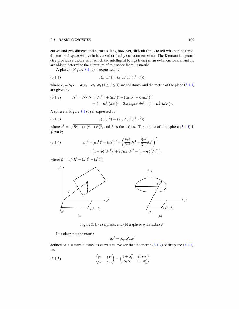
3.1. BASIC CONCEPTS 109
curves and two-dimensional surfaces. It is, however, difficult for us to tell whether the three-
dimensional space we live in is curved or flat by our common sense. The Riemannian geom-
etry provides a theory with which the intelligent beings living in an n-dimensional manifold
are able to determine the curvature of this space from its metric.
A plane in Figure 3.1 (a) is expressed by
(3.1.1) ~r(x1,x2) = (x1,x2,x3(x1,x2)),
where x3 =α1x1+α2x2+α3, α j (1≤ j ≤ 3) are constants, and the metric of the plane (3.1.1)
are given by
ds2 = d~r ·d~r =(dx1)2 +(dx2)2 +(α1dx1 +α2dx2)2(3.1.2)
=(1+α21)(dx1)2 + 2α1α2dx1dx2 +(1+α2
2)(dx2)2.
A sphere in Figure 3.1 (b) is expressed by
(3.1.3) ~r(x1,x2) = (x1,x2,x3(x1,x2)),
where x3 =√
R2 − (x1)2 − (x2)2, and R is the radius. The metric of this sphere (3.1.3) is
given by
ds2 =(dx1)2 +(dx2)2 +
(∂x3
∂x1dx1 +
∂x3
∂x2dx2
)2
(3.1.4)
=(1+ϕ)(dx1)2 + 2ϕdx1dx2 +(1+ϕ)(dx2)2,
where ϕ = 1/(R2 − (x1)2 − (x2)2).
x1
x2
x3
r
(x1, x2)
(a)
x1
x3
x2
r
(x1, x2)
(b)
Figure 3.1: (a) a plane, and (b) a sphere with radius R.
It is clear that the metric
ds2 = gi jdxidx j
defined on a surface dictates its curvature. We see that the metric (3.1.2) of the plane (3.1.1),
i.e.
(3.1.5)
(g11 g12
g21 g22
)=
(1+α2
1 α1α2
α1α2 1+α22
)
110 CHAPTER 3. MATHEMATICAL FOUNDATIONS
is a constant metric, and the metric (3.1.4) of the sphere (3.1.3), i.e.
(3.1.6)
(g11 g12
g21 g22
)=
(1+ϕ(x1,x2) ϕ(x1,x2)
ϕ(x1,x2) 1+ϕ(x1,x2)
)
is not constant. In fact, for the plane shown by Figure 3.1(a), we can find a coordinate
transformation
(x1
x2
)=
(a1
1 a12
a21 a2
2
)(x1
x2
),
such that in the coordinate system (x1, x2), the metric (3.1.2) is expressed in the diagonal
form:
(3.1.7) ds2 = (dx1)2 +(dx2)2.
In other words, the metric is gi j = δi j. However, it is impossible to achieve this for the metric
(3.1.4) of the sphere.
The conclusion in this example holds true as well for all Riemannian manifolds. Namely,
for a Riemannian manifold M ,gi j, M is flat if and only if there is a coordinate system x,
such that the metric gi j can be expressed as gi j = δi j under the x-coordinate system.
The following are a few general properties of an n-dimensional Riemannian manifold
M ,gi j.
1. The Riemannian metric
(3.1.8) ds2 = gi jdxidx j
is invariant. In fact, under a coordinate transformation
(3.1.9) x = ϕ(x), x = ϕ−1(x),
the second-order covariant tensor field gi j satisfies that
(gi j) = (bki )
T (gkl)(blj),
dx1
...
dxn
= (ai
j)
dx1
...
dxn
,
(aij) =
(∂ϕ i
∂x j
), (bi
j) = (aij)−1.
3.1. BASIC CONCEPTS 111
Hence we have
gi jdxidx j =(dx1, · · · ,dxn)(gi j)
dx1
...
dxn
(3.1.10)
=(dx1, · · · ,dxn)(aki )
T (bki )
T (gkl)(blj)(a
lj)
dx1
...
dxn
=(dx1, · · · ,dxn)(gi j)
dx1
...
dxn
=gi jdxidx j.
It follows that the metric (3.1.8) is invariant.
2. The length of a curve on M is determined by the metric gi j. Let γ(t) be a curve
connecting two points p,q ∈ M, and γ(t) be expressed by
(3.1.11) x(t) = (x1(t), · · · ,xn(t)), 0 ≤ t ≤ T, x(0) = p,x(T ) = q.
By (3.1.8) the infinitesimal arc-length is given by
ds =√
gi jdxidx j =√
gi j(x(t))xix jdt.
Hence the length L of γ(t) is given by
(3.1.12) L =
∫ q
pds =
∫ T
0
√gi j(x(t))
dxi
dt
dx j
dtdt.
The invariance of ds as shown in (3.1.10) implies that the length L in (3.1.12) is independent
of the coordinate systems.
3. The volume of a bounded domain U ⊂ M is invariant. The reason why gi j is called
a metric is that such quantities as the length, area, volume and angle are all determined by the
metric gi j.
Given a Riemannian manifold M ,gi j, let U ⊂ M be a bounded domain. Then the
volume of U is written as
(3.1.13) V =
∫
UΩ(x)dx.
where the volume element Ωdx reads
(3.1.14) Ω(x)dx =√−gdx, g = det(gi j).
To derive (3.1.14), let M ⊂ Rn+1 be an embedding, and
~r(x) = r1(x), · · · ,rn+1(x),
112 CHAPTER 3. MATHEMATICAL FOUNDATIONS
be the embedding function. Consider the vector product of n vectors in Rn:
[∂~r
∂x1, · · · , ∂~r
∂xn
]=
∣∣∣∣∣∣∣∣∣
~e1 · · · ~en+1
∂1r1 · · · ∂1rn+1
......
∂nr1 · · · ∂nrn+1
∣∣∣∣∣∣∣∣∣,
where ~e1, · · · ,~en+1 is an orthogonal basis of Rn+1. Then the volume element Ωdx is
Ωdx =
∣∣∣∣[
∂~r
∂x1, · · · , ∂~r
∂xn
]∣∣∣∣dx.
By gi j =∂~r∂xi · ∂~r
∂x j , the norm of the vector [∂1~r, · · · ,∂n~r] is
|[∂1~r, · · · ,∂n~r]|=√−g, g = det (gi j).
Thus (3.1.14) follows.
We now verify the invariance of the volume element. Under the transformation (3.1.9),
dx =dx1 ∧·· ·∧dxn(3.1.15)
=
(∂ϕ1
∂x1dx1 + · · ·+ ∂ϕ1
∂xndxn
)∧·· ·∧
(∂ϕn
∂x1dx1 + · · ·+ ∂ϕn
∂xndxn
)
=det
(∂ϕ i
∂x j
)dx1 ∧·· ·∧dxn.
On the other hand,
(3.1.16) (gi j) =
(∂ψ i
∂y j
)(gi j)
(∂ψ i
∂y j
)T
, ψ = ϕ−1.
Hence
(3.1.17)
√det(gi j) = det
(∂ϕ i
∂x j
)−1√det(gi j).
We deduce from (3.1.15) and (3.1.17) that
√det(gi j)dx =
√det(gi j)dx.
Namely, both the volume and the volume element in (3.1.13)-(3.1.14) are invariant.
4. The metric gi j gives rise to an inner product structure on the tangent space of a
Riemann manifold M , and defines the angle between two tangent vectors.
Let p ∈ M be a given point, and TpM be the tangent space at p ∈ M. For two vectors
X ,Y ∈ TpM ,
X = X1, · · · ,Xn, Y = Y 1, · · · ,Y n,
3.1. BASIC CONCEPTS 113
the inner product of X and Y is defined by
(3.1.18) 〈X ,Y 〉= gi j(p)X iY j.
It is clear that the inner product (3.1.18) is an invariant. The angle between X and Y is defined
as
cosθ =〈X ,Y 〉|X ||Y | , |Z|=
√gi jZiZ j for Z = X ,Y.
5. The inverse of (gi j), denoted by
(gi j) = (gi j)−1,
is a second order contra-variant tensor. In fact, by (3.1.16) we have that
I = (gi j)(gi j) =
(∂ϕ
∂x
)−1
(gi j)
[(∂ϕ
∂x
)T]−1
(gi j),
where I is unit matrix. It follows that
(gi j) =
(∂ϕ
∂x
)T
(gi j)
(∂ϕ
∂x
).
Hence gi j is a second-order contra-variant tensor.
3.1.2 Physical fields and vector bundles
Let M be a manifold. A vector bundle on M is obtained by gluing an N-dimensional linear
space EN at each point p ∈ M , denoted by
(3.1.19) M ⊗p EN def=
⋃
p∈M
p×ENp ,
where EN = RN , or CN , or the Minkowski space.
In a vector bundle (3.1.19), the geometric position of ENp is related with p ∈ M . For
example, the set of all tangent spaces is a vector bundle on M , called the tangent bundle of
M , denoted by
TM = M ⊗p TpM .
For (3.1.19), if the positions of bundle spaces ENp (p ∈ M ) are independent of p, then it
is called a geometrically trivial vector bundle. Vector bundles on a flat manifold are always
geometrically trivial.
The physical background of vector bundles are very clear. Each physical field must be
a mapping from the base space M to a vector bundle M ⊗p EN . Actually, all physical
events occur in the space-time universe M , and the physical fields describing these events
are defined on vector bundles. This point of view is well illustrated in the following examples.
114 CHAPTER 3. MATHEMATICAL FOUNDATIONS
Example 3.1. The motion of the air or seawater can be ideally considered as a fluid motion
on a two-dimensional sphere S2, and the velocity field u is defined on the tangent planes T S2:
u : S2 → TS2 with u(p) ∈ TpS2 ∀p ∈ S2.
Example 3.2. The electromagnetic interaction takes place on the 4D space-time manifold
M , and the electromagnetic field Aµ is defined on the tangent space:
Aµ : M → TM with Aµ(p) ∈ TpM ∀p ∈ M ,
where at each point p ∈ M , TpM is the Minkowski space.
Example 3.3. An electron moves in the space-time manifold M , and the field describing the
electron state is the Dirac spinor ψ , which is defined on a 4D complex space C4:
ψ : M → M ⊗p C4p with ψ(p) ∈C
4p ∀p ∈ M .
Examples 3.1-3.3 clearly illustrate that all physical fields are defined on a vector bundle
on M . Namely, a physical field F is a mapping:
(3.1.20) F : M → M ⊗p ENp with F(p) ∈ EN
p ∀p ∈ M .
The physical field F takes its values in the N-dimensional linear space EN , and can be
written as N components,
(3.1.21) F = (F1, · · · ,FN)T .
Considering invariance under certain symmetry, the transformation group always acts on
the bundle space EN , and induces a corresponding transformation for the field F in (3.1.21).
Also, in order to ensure the covariance of the field equations for F , a differential operator
D acting F must also be covariant, leading to the introduction of connections on the vector
bundle M ⊗p EN . This process is shown as follows:
1. Symmetric group G act on EN :
(3.1.22) Gp : ENp → EN
p .
2. The fields F induced to be transformed:
(3.1.23) F → TpF.
3. The vector bundle M ⊗p EN is endowed with connections Γµ :
(3.1.24) Dµ = ∂µ +Γµ .
Finally, we say that the vector bundle M ⊗p EN is geometrically trivial if and only if
the connections Γµ in (3.1.24) are zero, i.e. Γµ = 0 on M . It implies that the transforma-
tions (3.1.22)-(3.1.23) determines whether M ⊗p ENp is geometrically trivial, and if Gp,Tp
in (3.1.22) and (3.1.23) are independent of p ∈ M , then M ⊗p EN is geometrically trivial,
and otherwise it’s not. This viewpoint is important for the unified field theory introduced
in Chapter 4, because it implies that the geometry of M ⊗p EN is determined by symmetry
principles.
The other reason to adopt vector bundles as the mathematical framework to describe
physical fields F is that the types of F can be directly reflected by the bundle space EN .
Hereafter we list a few useful physical fields:
3.1. BASIC CONCEPTS 115
1) For a real (complex) scalar field φ , the associated vector bundle is M ⊗pR1 (M ⊗pC):
φ : M → M ⊗p R1 (M ⊗p C).
2) Let Aµ be a 4-dimensional vector field. Then
Aµ : M → TM ,
and for any p ∈ M , TpM is the Minkowski space.
3) For a 4-dimensional covector field Aµ , we have
Aµ : M → T ∗M ,
and for any p ∈ M , T ∗p M is the dual space of TpM .
4) A (k,r)-tensor field T on M :
T = Tµ1···µk
ν1···νr,
is expressed by
T : M → T kr M ,
where T kr M is the (k,r)-tensor bundle on M , denoted by
(3.1.25) T kr M = TM ⊗·· ·⊗TM︸ ︷︷ ︸
k
⊗T ∗M ⊗·· ·⊗T ∗
M︸ ︷︷ ︸r
,
and ⊗ represents the tensor product.
5) The Dirac spinor field Ψ is defined by
Ψ : M → M ⊗p C4.
In particular, for N Dirac spinor fields Ψ = (ψ1, · · · ,ψN)T ,
Ψ : M → M ⊗p (C4)N .
6) The Riemann metric gµν defined on a 4D space-time manifold M , representing the
gravitational potential, is a mapping:
gµν : M → T 02 M ,
where T 02 M = T ∗M ⊗T ∗M is a (0,2)-tensor bundle as defined by (3.1.25).
The fields given by 1)-6) above include all types of physical fields, and the associated
vector bundles are physically significant.
In classical theories of interactions, the physical fields and the associated bundle spaces
are given as follows:
1) Gravity:
(3.1.26) gµν : M → T ∗M ⊗T ∗
M .
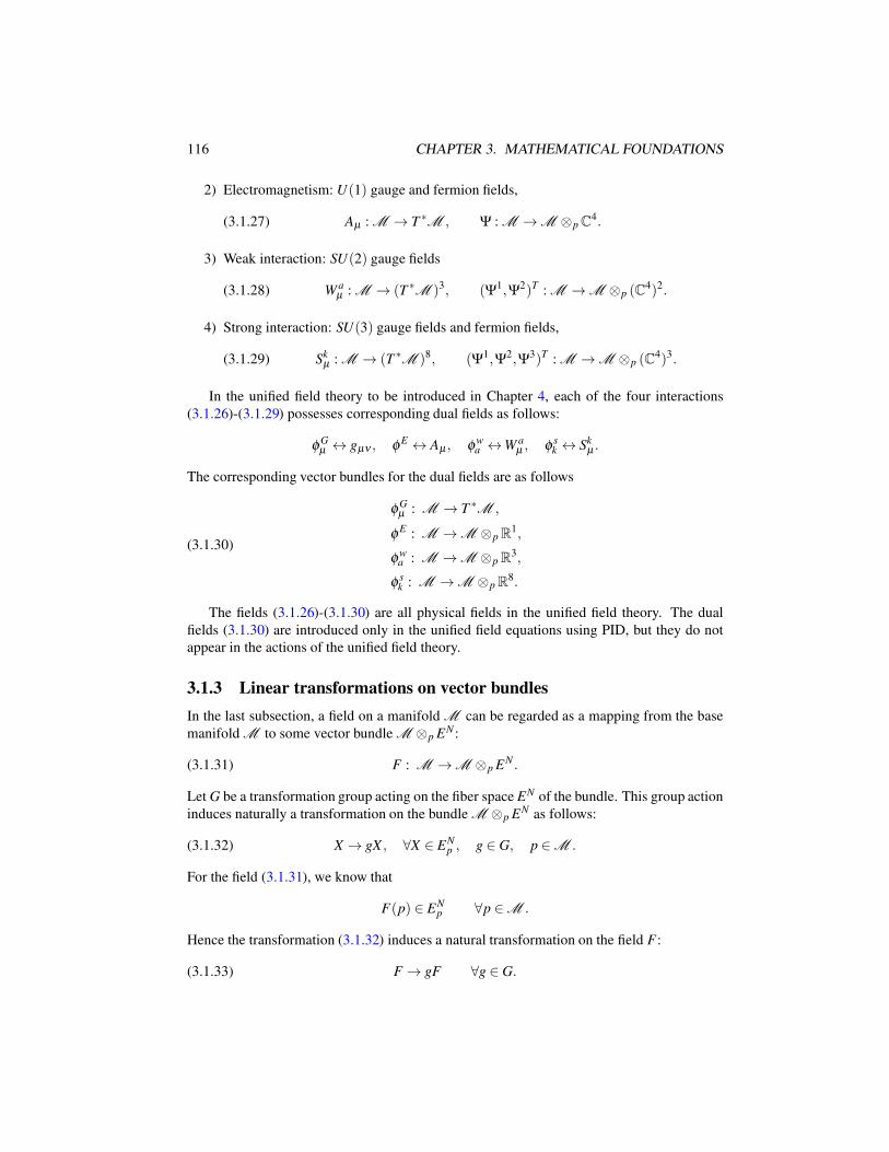
116 CHAPTER 3. MATHEMATICAL FOUNDATIONS
2) Electromagnetism: U(1) gauge and fermion fields,
(3.1.27) Aµ : M → T ∗M , Ψ : M → M ⊗p C
4.
3) Weak interaction: SU(2) gauge fields
(3.1.28) W aµ : M → (T ∗
M )3, (Ψ1,Ψ2)T : M → M ⊗p (C4)2.
4) Strong interaction: SU(3) gauge fields and fermion fields,
(3.1.29) Skµ : M → (T ∗
M )8, (Ψ1,Ψ2,Ψ3)T : M → M ⊗p (C4)3.
In the unified field theory to be introduced in Chapter 4, each of the four interactions
(3.1.26)-(3.1.29) possesses corresponding dual fields as follows:
φGµ ↔ gµν , φE ↔ Aµ , φw
a ↔W aµ , φ s
k ↔ Skµ .
The corresponding vector bundles for the dual fields are as follows
(3.1.30)
φGµ : M → T ∗
M ,
φE : M → M ⊗p R1,
φwa : M → M ⊗p R
3,
φ sk : M → M ⊗p R
8.
The fields (3.1.26)-(3.1.30) are all physical fields in the unified field theory. The dual
fields (3.1.30) are introduced only in the unified field equations using PID, but they do not
appear in the actions of the unified field theory.
3.1.3 Linear transformations on vector bundles
In the last subsection, a field on a manifold M can be regarded as a mapping from the base
manifold M to some vector bundle M ⊗p EN :
(3.1.31) F : M → M ⊗p EN .
Let G be a transformation group acting on the fiber space EN of the bundle. This group action
induces naturally a transformation on the bundle M ⊗p EN as follows:
(3.1.32) X → gX , ∀X ∈ ENp , g ∈ G, p ∈ M .
For the field (3.1.31), we know that
F(p) ∈ ENp ∀p ∈ M .
Hence the transformation (3.1.32) induces a natural transformation on the field F :
(3.1.33) F → gF ∀g ∈ G.
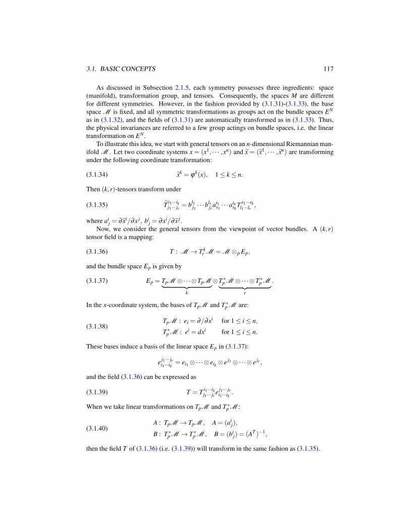
3.1. BASIC CONCEPTS 117
As discussed in Subsection 2.1.5, each symmetry possesses three ingredients: space
(manifold), transformation group, and tensors. Consequently, the spaces M are different
for different symmetries. However, in the fashion provided by (3.1.31)-(3.1.33), the base
space M is fixed, and all symmetric transformations as groups act on the bundle spaces EN
as in (3.1.32), and the fields of (3.1.31) are automatically transformed as in (3.1.33). Thus,
the physical invariances are referred to a few group actings on bundle spaces, i.e. the linear
transformation on EN .
To illustrate this idea, we start with general tensors on an n-dimensional Riemannian man-
ifold M . Let two coordinate systems x = (x1, · · · ,xn) and x = (x1, · · · , xn) are transforming
under the following coordinate transformation:
(3.1.34) xk = ϕk(x), 1 ≤ k ≤ n.
Then (k,r)-tensors transform under
(3.1.35) Ti1···ikj1··· jr = b
l1j1· · ·blr
jrai1
s1· · ·aik
skT
s1···sk
l1···lr ,
where aij = ∂ xi/∂x j, bi
j = ∂xi/∂ x j.Now, we consider the general tensors from the viewpoint of vector bundles. A (k,r)
tensor field is a mapping:
(3.1.36) T : M → T kr M = M ⊗p Ep,
and the bundle space Ep is given by
(3.1.37) Ep = TpM ⊗·· ·⊗TpM︸ ︷︷ ︸k
⊗T ∗p M ⊗·· ·⊗T ∗
p M︸ ︷︷ ︸
r
.
In the x-coordinate system, the bases of TpM and T ∗p M are:
(3.1.38)TpM : ei = ∂/∂xi for 1 ≤ i ≤ n,
T ∗p M : ei = dxi for 1 ≤ i ≤ n.
These bases induce a basis of the linear space Ep in (3.1.37):
ej1··· jri1···ik = ei1 ⊗·· ·⊗ eik ⊗ e j1 ⊗·· ·⊗ e jr ,
and the field (3.1.36) can be expressed as
(3.1.39) T = Ti1···ikj1··· jr e
j1··· jri1···ik .
When we take linear transformations on TpM and T ∗p M :
(3.1.40)A : TpM → TpM , A = (ai
j),
B : T ∗p M → T ∗
p M , B = (bij) = (AT )−1,
then the field T of (3.1.36) (i.e. (3.1.39)) will transform in the same fashion as (3.1.35).
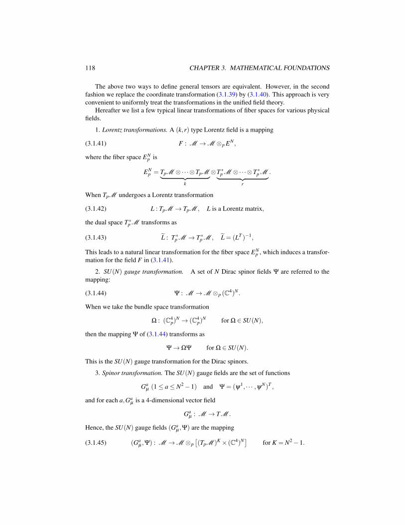
118 CHAPTER 3. MATHEMATICAL FOUNDATIONS
The above two ways to define general tensors are equivalent. However, in the second
fashion we replace the coordinate transformation (3.1.39) by (3.1.40). This approach is very
convenient to uniformly treat the transformations in the unified field theory.
Hereafter we list a few typical linear transformations of fiber spaces for various physical
fields.
1. Lorentz transformations. A (k,r) type Lorentz field is a mapping
(3.1.41) F : M → M ⊗p EN ,
where the fiber space ENp is
ENp = TpM ⊗·· ·⊗TpM︸ ︷︷ ︸
k
⊗T ∗p M ⊗·· ·⊗T∗
p M︸ ︷︷ ︸
r
.
When TpM undergoes a Lorentz transformation
(3.1.42) L : TpM → TpM , L is a Lorentz matrix,
the dual space T ∗p M transforms as
(3.1.43) L : T ∗p M → T ∗
p M , L = (LT )−1,
This leads to a natural linear transformation for the fiber space ENp , which induces a transfor-
mation for the field F in (3.1.41).
2. SU(N) gauge transformation. A set of N Dirac spinor fields Ψ are referred to the
mapping:
(3.1.44) Ψ : M → M ⊗p (C4)N .
When we take the bundle space transformation
Ω : (C4p)
N → (C4p)
N for Ω ∈ SU(N),
then the mapping Ψ of (3.1.44) transforms as
Ψ → ΩΨ for Ω ∈ SU(N).
This is the SU(N) gauge transformation for the Dirac spinors.
3. Spinor transformation. The SU(N) gauge fields are the set of functions
Gaµ (1 ≤ a ≤ N2 − 1) and Ψ = (ψ1, · · · ,ψN)T ,
and for each a,Gaµ is a 4-dimensional vector field
Gaµ : M → TM .
Hence, the SU(N) gauge fields (Gaµ ,Ψ) are the mapping
(3.1.45) (Gaµ ,Ψ) : M → M ⊗p
[(TpM )K × (C4)N
]for K = N2 − 1.
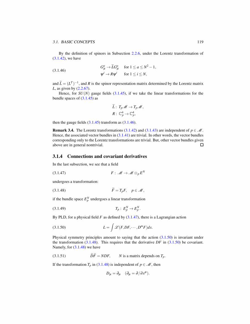
3.1. BASIC CONCEPTS 119
By the definition of spinors in Subsection 2.2.6, under the Lorentz transformation of
(3.1.42), we have
(3.1.46)Ga
µ → LGaµ for 1 ≤ a ≤ N2 − 1,
ψ i → Rψ i for 1 ≤ i ≤ N,
and L = (LT )−1, and R is the spinor representation matrix determined by the Lorentz matrix
L, as given by (2.2.67).
Hence, for SU(N) gauge fields (3.1.45), if we take the linear transformations for the
bundle spaces of (3.1.45) as
L : TpM → TpM ,
R : C4p →C
4p,
then the gauge fields (3.1.45) transform as (3.1.46).
Remark 3.4. The Lorentz transformations (3.1.42) and (3.1.43) are independent of p ∈ M .
Hence, the associated vector bundles in (3.1.41) are trivial. In other words, the vector bundles
corresponding only to the Lorentz transformations are trivial. But, other vector bundles given
above are in general nontrivial.
3.1.4 Connections and covariant derivatives
In the last subsection, we see that a field
(3.1.47) F : M → M ⊗p EN
undergoes a transformation:
(3.1.48) F = TpF, p ∈ M ,
if the bundle space ENp undergoes a linear transformation
(3.1.49) Tp : ENp → EN
p .
By PLD, for a physical field F as defined by (3.1.47), there is a Lagrangian action
(3.1.50) L =
∫L (F,DF, · · · ,DmF)dx.
Physical symmetry principles amount to saying that the action (3.1.50) is invariant under
the transformation (3.1.48). This requires that the derivative DF in (3.1.50) be covariant.
Namely, for (3.1.48) we have
(3.1.51) DF = NDF, N is a matrix depends on Tp.
If the transformation Tp in (3.1.48) is independent of p ∈ M , then
Dµ = ∂µ (∂µ = ∂/∂xµ).
120 CHAPTER 3. MATHEMATICAL FOUNDATIONS
However, if Tp depends on p ∈ M, then we have
(3.1.52) ∂µ(TpF) = Tp∂µ F + ∂µTpF,
which violates the covariance of (3.1.51), because it has a superfluous term ∂µTpF in the
right-hand side of (3.1.52). Hence, the derivative operator Dµ must be in the form
(3.1.53) Dµ = ∂µ +Γµ ,
such that (3.1.51) holds true. The field Γµ is the connection of the vector bundle M ⊗p EN
under the transformation (3.1.49).
To make explicit of Γµ , we assume that ∂µ and ∂µ have the following relation
(3.1.54) ∂µ = A∂µ ,
and A is a matrix in the following form
(3.1.55) A =
identity for SU(N) gauge fields,
Lorentz matrix for Lorentz tensors,
affine matrix for general tensors.
By (3.1.48) and (3.1.53)-(3.1.54), we have
Dµ F = (∂µ + Γµ)(TpF) = ATp∂µF +A∂µTpF + ΓµTpF.
Thanks to (3.1.51),
N(∂µ +Γµ)F = ATp∂µF +A∂µTpF + ΓµTpF.
It follows that
N = ATp, Γµ = ATpΓµ T−1p −A∂µTpT−1
p .
In other words, under the linear transformation (3.1.49), the system transforms as follows
(3.1.56)DF = (ATp)DF,
Γ = ATpΓT−1p −A(∂Tp)T
−1p .
The following summarizes the connections of all symmetry transformations:
1. Connection for Lorentz group. As the Lorentz transformation Tp is independent of
p ∈ M , the connections Γµ are zero:
Γµ = 0 for the Lorentz action.
2. Connection for SU(N) group. For the SU(N) group action, (3.1.49) is
Ωp : (C4)N → (C4)N , Ωp ∈ SU(N), p ∈ M .
3.1. BASIC CONCEPTS 121
By (3.1.55), A = I. The connection of SU(N) group is the gauge fields Gaµ :
Γµ =
igGaµτa | τaN2−1
a=1 is a set of generators of SU(N).
Hence, relations (3.1.56) for the SU(N) gauge fields Gaµ are written as
DΨ = ΩΨ, Ψ : M → M⊗p (C4)N ,
Gaµτa = ΩGa
µτaΩ−1 − 1
ig∂ΩΩ−1, Ω ∈ SU(N).
3. Connections for general linear group GL(n). For (k,r)-tensors:
(3.1.57) F : M → T kr M ,
the GL(n) group action
(3.1.58) Ap : TM → TM , Ap ∈ GL(n),
induces a linear transformation:
(3.1.59) Tp = Ap ⊗·· ·⊗Ap︸ ︷︷ ︸k
⊗A−1p ⊗·· ·⊗A−1
p︸ ︷︷ ︸r
: T kr M → T k
r M ,
which can be equivalently expressed a K ×K matrix with K = nk+r, and ⊗ is the tensor
product of matrices defined by (3.1.67); see Remark 3.5. In this case, the matrix A of (3.1.54)-
(3.1.55) is precisely the Ap in (3.1.58). Hence, by (3.1.56) we have
(3.1.60) DF = (A⊗T)DF,
where F is as in (3.1.57), T is as in (3.1.59), and A is as in (3.1.58).
The covariant derivative operator D depends on the indices k and r of bundle spaces T kr M,
and are derived by induction.
4. Derivative on TM . For F = (F1, · · · ,Fn),
(3.1.61) D jFi = ∂ jF
i +ΓijlF
l ,
where Γijl are connections defined on TM . As M is a Riemannian manifold, Γi
jk are the
Levi-Civita connection as given by (2.3.25). It follows from (3.1.56) that the connection of
(3.1.61) transforms as
(3.1.62) Γ = A⊗A⊗ (AT)−1Γ−A⊗ ∂A⊗A−1,
which is the the same as those of (2.3.23).
5. Derivative on T ∗M . Consider F = (F1, · · · ,Fn). The derivative operators satisfy that
(3.1.63)D(A ·B) = DA ·B+A ·DB,
D(A⊗B) = DA⊗B+A⊗DB.
122 CHAPTER 3. MATHEMATICAL FOUNDATIONS
It is known that
(3.1.64) FkGk = a scalar field, and D(FkGk) = ∂ (FkGk).
We infer then from (3.1.63) and (3.1.64) that
(3.1.65) DkFiGi +FiDkGi = ∂kFiG
i +Fi∂kGi.
Inserting (3.1.61) in (3.1.65) we deduce that
DkFi = ∂kFi −Γ jkiFj.
6. Derivative on T kr M . For two vector fields Ak and Bk, their tensor product A⊗B =
AiB j is a second order tensor. By (3.1.63) we have
Dk(A⊗B) =Dk(AiB j) = DkAiB j +AiDkB j
=(∂kAi +ΓiklA
l)B j +Ai(∂kB j +Γ jklB
l)
=∂k(AiB j)+Γi
klAlB j +Γ
j
klAiBl .
Replacing A⊗B by T i j, we obtain
DkT i j = ∂kT i j +ΓiklT
l j +Γj
klTil .
In the same fashion, for general (k,r)-tensors
T = Ti1···ikj1··· jr : M → T k
r M ,
its covariant derivative can be expressed as
DkTi1···ikj1··· jr =∂kT
i1···ikj1··· jl +Γi1
klTli2···ikj1··· jr
+ · · ·+(3.1.66)
+ΓikklT
i1···ik−1l
j1··· jr −Γlk j1
Ti1···ikj2··· jr −·· ·−Γl
k jrTi1···ikj1··· jk−1l .
The derivative (3.1.66) were given in (2.3.26).
Remark 3.5. We have encountered tensor products in (3.1.59) and (3.1.62). A further expla-
nation of this considered is now in order. Let A and B be two matrices with orders n and m
respectively. Then A⊗B is a matrix of order N = nm, defined by
(3.1.67) A⊗B =
a11B · · · a1nB...
...
an1B · · · annB
, ai jB =
ai jb11 · · · ai jb1m
......
ai jbm1 · · · ai jbmm
.
In (3.1.60) and (3.1.62), the components of DF = DkFi1···ikj1··· jr and Γ = Γk
i j are arranged to
be in two vectorial forms.
3.2. ANALYSIS ON RIEMANNIAN MANIFOLDS 123
3.2 Analysis on Riemannian Manifolds
3.2.1 Sobolev spaces of tensor fields
The gravitational field equations are defined on a Riemannian manifold. To study these equa-
tions, it is necessary to introduce various types of function spaces on manifolds, which pos-
sess different differentiability. In particular, we need to introduce the concept of weak deriva-
tives.
Let M be an n-dimensional manifold with metric gi j. The following functions are
defined on M .
1. Lp spaces. For a real number p (1 ≤ p < ∞), we denote
(3.2.1) Lp(M ⊗p EN) =
u : M → M ⊗p EN
∣∣∣∫
M
|u|p√−gdx < ∞
,
where√−gdx is the volume element, and |u| is the modulus of u. For example, if u : M →
TM is a vector field, then
|u|= |gi juiu j|1/2.
The space (3.2.1) is endowed with Lp-norm as
||u||Lp =
[∫
M
|u|p√−gdx
]1/p
.
By Functional Analysis, the spaces Lp(M ⊗p EN) are Banach spaces, and for 1 < p < ∞,
Lp(M ⊗p EN) are reflective and separable. The dual spaces of Lp(M ⊗p EN) (1 < p < ∞)are
Lp(M ⊗p EN)∗ = Lq(M ⊗p (EN)∗),
Lq(M ⊗p EN)∗ = Lp(M ⊗p (EN)∗),
1
p+
1
q= 1,
where (EN)∗ is the dual space of EN .
For p = ∞, we define that
L∞(M ⊗p EN) = u : M → M ⊗p EN | u is bounded almost everywhere.
The norm of L∞(M ⊗p EN) is defined by
||u||L∞ = supM
|u|.
The space L∞(M ⊗p EN) is a Banach space, but not reflective and separable. The space
L∞(M ⊗p EN) is the dual space of L1(M ⊗p EN), i.e.
L1(M ⊗p EN)∗ = L∞(M ⊗p (EN)∗).
2. Weakly differentiable functions. A field u ∈ Lp(M ⊗p EN) is called k-th order weakly
differentiable, if each component u j is k-th order weakly differentiable, i.e. for each u j there
exists uniquely a function ϕ such that for all v ∈C∞0 (M ) we have
(3.2.2)
∫
M
ϕv√−gdx = (−1)k
∫
M
u j∂kvdx.
124 CHAPTER 3. MATHEMATICAL FOUNDATIONS
In this case, ϕ is called the k-th weak derivative of u j, denoted by
(3.2.3) ϕ = ∂ ku j.
The space C∞0 (M ) consists of infinitely differentiable functions, and
(3.2.4) C∞0 (M ) =
C∞(M ) if M is compact and ∂M = /0,
u ∈C∞(M )| u 6= 0 in a compact set of M .
The definition (3.2.2)-(3.2.3) for weak derivatives is very abstract. In the following, we
discuss the distinction between continuity and weak differentiability in an intuitive fashion.
Let u be a function defined on Rn. It is known that if u is differentiable at x = 0, then u
can be Taylor expanded as
(3.2.5) u(x) = ax+ o(|x|),
where a = ∇u(0) is the first order derivative of u at x = 0, i.e. the gradient of u at x = 0.
However, if u is weakly but not continuously differentiable at x = 0, then in a neighbor-
hood of x = 0,u must contain at least a term as |xi|α (α ≤ 1). Without loss of generality, we
express u in the form
(3.2.6) u = a|x|α + continuously differentiable terms,
where a 6= 0 is a constant, and 1−n<α ≤ 1. The index α in (3.2.6) determines the regularity
of u as follows:
(3.2.7)
u = Lipschitz if α = 1,
u = Holder if 0 < α < 1,
u = singularity if α < 1.
Expressions (3.2.5) and (3.2.6) exhibit the essential difference between continuity and
weak differentiability.
Remark 3.6. For a weakly differentiable function as (3.2.6), its index α has to satisfy 1−n<α ≤ 1, which is crucial in the Sobolev embedding theorems in the next subsection.
3. W k,p spaces (Sobolev spaces). Let u : M → M ⊗p EN . Then, u = u j| 1 ≤ j ≤ N,
and each component u j of u is a function on M. We denote
∂ α u j =∂ ku j
(∂x1)α1 · · ·(∂xn)αnfor α = (α1, · · · ,αn),
and k = |α|=n
∑i=1
αi (αi ≥ 0). Then, we define W k,p spaces as
(3.2.8) W k,p(M ⊗p EN) = u ∈ Lp(M ⊗p EN)| ∂ β u j ∈ Lp(M ), 1 ≤ j ≤ n, 0 ≤ β ≤ k,
and ∂ β u j in (3.2.8) are weak derivatives of u j.
3.2. ANALYSIS ON RIEMANNIAN MANIFOLDS 125
The spaces W k,p(M ⊗p EN) are called Sobolev spaces, and the norms are defined by
(3.2.9) ||u||W k,p =k
∑β=0
[∫
M
|Dβ u|p√−gdx
]1/p
.
It is clear that
u ∈W k,p(M ⊗p EN) ⇒ u is k− th weakly differentiable.
In addition, we introduce the spaces Wk,p0 (M ⊗p EN) as
Wk,p0 (M ⊗p EN) = Closure of C∞
0 (M ⊗p EN) under W k,p norm (3.2.9).
Here C∞0 (M ⊗p EN) is as defined in (3.2.4).
If ∂M = /0, then Wk,p0 (M ⊗p EN) = W k,p(M ⊗p EN), and if ∂M 6= /0 then for u ∈
Wk,p0 (M ⊗p EN) we have
u|∂M = 0, · · · , ∂ β u|∂M = 0 ∀|β | ≤ k− 1.
4. Hk spaces. As M is a Riemannian manifold, M ⊗p EN and its dual bundle M ⊗p
(EN)∗ are isomorphic. In this case, the spaces W k,2(M ⊗p EN) are Hilbert spaces, denoted
by
(3.2.10)Hk(M ⊗p EN) =W k,2(M ⊗p EN),
Hk0(M ⊗p EN) =W
k,20 (M ⊗p EN).
The inner products of (3.2.10) are defined by
〈u,v〉Hk =
∫
M
k
∑|β |=0
Dβ u ·Dβ v∗√−gdx
where v∗ ∈ Hk(M ⊗p (EN)∗) is the dual field of v ∈ Hk(M ⊗p EN).
5. Lipschitz spaces. Let k ≥ 0 be integrals. The Lipschitz space Ck,1(M ⊗p EN) consists
of all k-th order continuously differentiable functions u with Dku being Lipschitz continuous:
Ck,1(M ⊗p EN) = u ∈Ck(M ⊗p EN)| [∂ ku]Lip < ∞,
where [∂ ku]Lip is the Lipschitz modulus, defined by
[v]Lip = supx,y∈M , x6=y
|v(x)− v(y)||x− y| .
A Lipschitz continuous function u∈C0,1(M ⊗p EN) is as shown in (3.2.6)-(3.2.7) with α = 1.
6. Holder spaces. The Holder space Ck,α(M ⊗p EN) (0 < α < 1) consists of all k-th
order continuously differentiable functions u with Dku being Holder continuous:
Ck,α (M ⊗p EN) = u ∈Ck(M ⊗p EN)| [Dku]α < ∞,
126 CHAPTER 3. MATHEMATICAL FOUNDATIONS
and [v]α is the Holder modulus:
[v]α = supx,y∈M , x6=y
|v(x)− v(y)||x− y|α , 0 < α < 1.
A Holder continuous function u ∈ C0,α(M ⊗p EN) is as shown in (3.2.6)-(3.2.7) with 0 <α < 1.
The norm of Ck,α(M ⊗p EN)(0 < α ≤ 1) is given by
||u||Ck,α = ||u||Ck +[Dku]α (0 < α ≤ 1),
where || · ||Ck is the norm of Ck(M ⊗p EN):
||u||Ck =k
∑|β |=0
supM
|∂ β u|.
3.2.2 Sobolev embedding theorem
In (3.2.6)-(3.2.7) we see that for Ω ⊂Rn, a function u∈W 1,p(Ω) does’t imply that u∈ Lq(Ω)for any q > p. For example, for the function
u = |x|−α , 0 < α <1
2, x ∈ Ω ⊂ R
3, Ω bounded,
it is known that
∇u = |x|− α+42 x ∈ L2(Ω).
Obviously we have
u ∈W 1,2(Ω), u 6∈ Lq(Ω) ∀q >n
α.
The following embedding problem of Sobolev spaces provides a solution for this problem.
Theorem 3.7 (Sobolev Embedding Theorem). Let M be an n-dimensional compact mani-
fold. Then we have the embeddings:
(3.2.11) W 1,p(M ⊗p EN) →
Lq(M ⊗p EN) for 1 ≤ q ≤ np
n− pif n > p,
Lq(M ⊗p EN) for 1 ≤ q < ∞ if n = p,
C0,α(M ⊗p EN) for α = 1− n/p if n < p.
Here C0,α(M ⊗p EN) are the Holder spaces. Moreover we have the following inequalities
for the norms:
(3.2.12)
||u||Lq ≤C||u||W 1,p for 1 ≤ q ≤ np
n− pif n > p,
||u||Lq ≤C||u||W 1,p for 1 ≤ q < ∞ if n = p,
||u||C0,α ≤C||u||W1,p for α = 1− n/p if n < p,
where C > 0 are constants depending on n, p and M.
3.2. ANALYSIS ON RIEMANNIAN MANIFOLDS 127
Remark 3.8. When M is non-compact, the conclusions (3.2.11) and (3.2.12) are also valid
only for q satisfying
p ≤ q ≤ np
n− pif n > p,
p ≤ q < ∞ if n = p.
Remark 3.9. By the recurrence relations
W k,p(M ⊗p EN) →W k−1,q(M ⊗p EN),
we readily deduce from (3.2.11) that
W k,p(M ⊗p EN) →
Lq(M ⊗p EN) for 1 ≤ q ≤ np
n− kpif n > kp,
Lq(M ⊗p EN) for 1 ≤ q < ∞ if n = kp,
CM ,α (M⊗p EN) for m+α = k− n/p if n < kp.
Based on weakly differentiability properties (3.2.6) and (3.2.7), essence of Theorem 3.7
can be seen from embeddings (3.2.11) using the following function:
(3.2.13) u(x) =|x|α
| ln |x||β , x ∈ Rn,
where β > 1 is given, and the exponent α < 1 is to reflect the critical embedding index q∗ in
(3.2.11).
The derivatives of u given by (3.2.13) are as follows
(3.2.14)
∇u = (∂1u, · · · ,∂nu),
∂iu =
(α
| ln |x||β − β
| ln |x||β+1
)|x|α−2xi.
Let BR = x ∈Rn| |x|< R, 0 < R < 1. Assume that
u ∈W 1,p(BR) for some 1 ≤ p < ∞.
Then, by (3.2.14) we have
(3.2.15)
∫
BR
|∇u|pdx ≤C
∫
BR
|x|(α−1)p
| ln |x||β pdx.
In the spherical coordinate system,
dx = rn−1drds,
and ds is the area element of the unit sphere, (3.2.15) becomes
∫
BR
|∇u|pdx ≤C
∫ R
0
∫
Sn−1
rn+(α−1)p−1
| lnr|β pdrds ≤C
∫ R
0
rk
| ln |r||β pdr,(3.2.16)
128 CHAPTER 3. MATHEMATICAL FOUNDATIONS
for 0 < R < 1 and β p > 1. It follows from (3.2.16) that
∫
BR
|∇u|pdx < ∞ ⇔ k = n+(α − 1)p− 1≥−1.
Hence we obtain that
(3.2.17) u =|x|α
| ln |x||β ∈W 1,p(BR) ⇔ α ≥ 1− n
p.
On the other hand, in the same fashion we see that
(3.2.18) u =|x|α
| ln |x||β ∈ Lq(BR) ⇔ α ≥−n
q.
Hence, by (3.2.17) we can see that as p > n,
u ∈C0,α(BR), α = 1− n
p,
and as p ≤ n, then from (3.2.17) and (3.2.18), at the critical embedding exponent q∗ we have
α = 1− n
p, α =− n
q∗.
It follows that
q∗
=np
n− pfor n > p
< ∞ for n = p.
Thus, we deduce that
(3.2.19) u ∈W 1,p(BR) ⇒
u ∈ Lq(BR) for 1 ≤ q ≤ np
n− pif n > p,
u ∈ Lq(BR) for 1 ≤ q < ∞ if n = p,
u ∈C0,α(BR) for α = 1− n
pif p > n.
The relations (3.2.19) are the embeddings given by (3.2.11).
3.2.3 Differential operators
A differential operator defined on a manifold M is a mapping given by
G : W k,p(M ⊗p EN11 ) → Lp(M ⊗p E
N22 ) for some k ≥ 1,
and is called a k-th order differential operator.
The most important operators in physics are:
1) the gradient operator: ∇,
2) the divergent operator: div,
3.2. ANALYSIS ON RIEMANNIAN MANIFOLDS 129
3) the Laplace operator: DkDk = div ·∇,
4) the Laplace-Beltrami operator: ∆ = dδ + δd,
5) the wave operator: = DµDµ , with Dµ being the 4-D gradient operator.
We now give a detailed account on the above operators.
1. Gradient operator. The gradient operator ∇ is a mapping of the following types:
(3.2.20)∇k : W 1,p(T k
r M )→ Lp(T k+1r M ),
∇k : W 1,p(T kr M )→ Lp(T k
r+1M ),
and ∇k and ∇k have the relation
∇k = gkl∇l , ∇k = gkl∇l ,
and gkl the Riemann metric of M . ∇ is expressed as
(3.2.21)∇k = (D1, · · · ,Dn),
D j the covariant derivative operators.
2. Divergence operator. The divergence operator div is a mapping of the following types:
(3.2.22)div : W 1,p(T k+1
r M )→ Lp(T kr M ),
div : W 1,p(T kr+1M )→ Lp(T k
r M ).
For T = Ti1···ik+1
j1··· jr ∈W 1,p(T k+1r M ) and T = T
i1···ikj1··· jr+1
∈W 1,p(T kr+1M),
(3.2.23)div T = Dil T
i1···il ···ik+1
j1··· jr , and
div T = D jl Ti1···ikj1··· jl ··· jk+1
As u ∈ W 1,p(TM ) and u ∈ W 1,p(T ∗M ), we can give the expressions of div u in the
following.
Let u ∈W 1,p(TM ),u = (u1, · · · ,un). Then by (3.2.23),
div u = Dkuk =∂uk
∂xk+Γk
k juj.
By the Levi-Civita connections (2.3.25), the contraction
Γkk j =
1
2gkl ∂gkl
∂x j=
1
2g
∂g
∂x j=
1√−g
∂√−g
∂x j,
here g = det (gi j). Thus we have
(3.2.24) div u =∂uk
∂xk+
1√−g
∂√−g
∂xkuk =
1√−g
∂ (√−guk)
∂xk.
130 CHAPTER 3. MATHEMATICAL FOUNDATIONS
Let u ∈W 1,p(T ∗M ),u = (u1, · · · ,un). Then,
div u =Dkuk = gklDl(uk) = Dl(glkuk)
=(by (3.2.24))
=1√−g
∂
∂xl(√−gglkuk).(3.2.25)
The formula (3.2.24) and (3.2.25) give expression of div u as:
(3.2.26) div u =
1√−g
∂
∂xk(√−guk) for u ∈W 1,p(TM ),
1√−g
∂
∂xk(√−ggklul) for u ∈W 1,p(T ∗
M ).
3. Laplace operators. The Laplace operator DkDk in Rn is in the familiar form
DkDk =∂
∂xk
∂
∂xk.
However, the Laplace operators DkDk defined on a Riemannian manifold are usually very
complex.
By (3.2.20) and (3.2.22), we have
W 2,p(T kr M )
∇k→W 1,p(T kr+1M )
div→ Lp(T kr M ),
W 2,p(T kr M )
∇k
→W 1,p(T k+1r M )
div→ Lp(T kr M ).
Hence, the Laplace operator div ·∇ is the mapping:
(3.2.27) div ·∇ : W 2,p(T kr M )→ Lp(T k
r M ).
By (3.2.21) and (3.2.23), div ·∇ is written as
div ·∇ = DkDk = gklDkDl .
4. Expression of div ·∇ on M ⊗p R1. A scalar field u on M can be regarded as u : M →
M ⊗p R1. In this case, ∇u is written as
∇u =
(∂u
∂x1, · · · , ∂u
∂xn
).
By (3.2.26), we get that
(3.2.28) div ·∇u =1√−g
∂
∂xk
(√−ggkl ∂u
∂xl
).
5. Expression of div ·∇ on TM . A vector field u : M → TM can be written as
u = (u1, · · · ,un),
3.2. ANALYSIS ON RIEMANNIAN MANIFOLDS 131
and its gradient (i.e. covariant derivatives) read as
(3.2.29)
∇u = Dkui,
Dkui =∂ui
∂xk+Γi
klul ,
and the divergence of ∇u is
div ·∇ui =DkDkui = gklDl(Dkui) = gkl
[∂
∂xl(Dkui)+Γi
l jDku j −Γ jklD ju
i
].
Then, by (3.2.29) we obtain that
div ·∇u =gkl
[∂
∂xl
(∂ui
∂xk+Γi
k juj
)+Γi
l j
(∂u j
∂xk+Γ j
ksus
)−Γ j
kl
(∂ui
∂x j+Γi
jsus
)].(3.2.30)
6. Laplace-Beltrami operators. The Laplace-Beltrami operators are defined by
∆ = dδ + δd,
where d is the differential operator, and δ the Hodge operator, which are defined on the spaces
of all differential forms. For a scalar field, ∆ is the same as div ·∇, i.e.
∆u = div ·∇u, as u ∈W 2,p(M ⊗p R1).
For vector fields and covector fields, we have
(3.2.31)∆ui =−div(∇ui)− gi jR jkuk,
∆ui =−div(∇u j)− gk jRi juk,
where Ri j is the Ricci curvature tensor defined by (2.3.31), and in (3.2.30) we give the formula
of div (∇uk). The expression of div (∇ui) is written as
div (∇ui) =gkl
∂
∂xl
[∂ui
∂xk−Γ j
iku j
]−Γ j
lk
[∂ui
∂x j−Γr
i jur
]−Γ j
li
[∂u j
∂xk−Γr
jkur
].(3.2.32)
Physically, it suffices to introduce the Laplace-Beltrami operators ∆ only for vector and
covector fields, i.e. the formula in (3.2.31).
Remark 3.10. The Navier-Stokes equations governing a fluid flow on a sphere (e.g. the
surface of a planet) are expressed in the spherical coordinate system, and the viscosity dif-
ferential operators are the Laplace-Beltrami operators given by (3.2.31); see Chapter 7 for
details.
3.2.4 Gauss formula
If M = Rn, it is known that the Gauss formula is∫
Rnu ·∇ f dx =−
∫
Rnf div udx ∀u ∈ H1 (Rn ×R
n), f ∈ H1(Rn),
132 CHAPTER 3. MATHEMATICAL FOUNDATIONS
which can be generalized to tensor fields on Riemann manifolds.
Let M be a Riemannian manifold with ∂M = /0. Then, there is an inner product defined
on TM defined by
(X ,Y ) = gi jXiX j ∀X ,Y ∈ TM .
Also, there is an inner product on T ∗M:
(X∗,Y ∗) = gi jX∗i Y ∗
j ∀X∗,Y ∗ ∈ T ∗M .
The tensor bundle T kr M is
T kr M = TM ⊗·· ·⊗TM︸ ︷︷ ︸
k
⊗T ∗M ⊗·· ·⊗T ∗
M︸ ︷︷ ︸r
.
The inner products on TM and T ∗M induce a natural inner product on T kr M :
(3.2.33) (u,v) = gi1 j1 · · ·gik jk gl1s1 · · ·glrsr ui1···ikl1···lr v j1··· jr
s1···sr∀u,v ∈ T k
r M .
Hence we can define the inner product 〈·, ·〉 on L2(T kr M ) by
(3.2.34) 〈u,v〉L2 =
∫
M
(u,v)√−gdx ∀u,v ∈ L2(T k
r M ),
where (u,v) is as in (3.2.33).
Furthermore, we can also define an inner product on the spaces Hm(T kr M ) as follows
(3.2.35) 〈u,v〉Hm =
∫
M
[(−1)m(∆mu,v)+ (u,v)]√−gdx ∀u,v ∈ Hm(T k
r M ),
where ∆ = div ·∇.In the following, we give the Gauss formula on T k
r M , which are crucial for the orthogonal
decomposition theory in the next section.
Theorem 3.11 (Gauss Formula). For any u ∈ H1(T kr M ) and v ∈ H1(T k+1
r M ) (or v ∈H1(T k
r+1M )),
(3.2.36)
∫
M
(∇u,v)√−gdx =−
∫
M
(u,divv)√−gdx.
Formula (3.2.36) is a corollary of the classical Gauss formula
(3.2.37)
∫
M
div w√−gdx =
∫
∂M
w ·nds.
In fact, let wk = (u,vk), then by (2.3.28) we have
div w = Dk(u,vk) = (∇u,v)+ (u,div v).
If ∂M = /0, then we derive from (3.2.37) that
∫
M
div w√−gdx =
∫
M
[(∇u,v)+ (u,div v)]√−gdx = 0,
3.2. ANALYSIS ON RIEMANNIAN MANIFOLDS 133
which is the formula (3.2.36).
The Gauss formula (3.2.36) can be generalized to more general gradient and divergent
operators, denoted by DA and divA.
Let A be a vector field or a covector field, and u ∈ L2(T kr M ). We define the operators DA
and divA by
(3.2.38)DAu = Du+ u⊗A,
divAu = divu− u ·A.
Based on (3.2.36), it is readily to verify that the following formula holds true for the operators
(3.2.38).
(3.2.39)
∫
M
(DAu,v)√−gdx =−
∫
M
(u,divAv)√−gdx.
Remark 3.12. The motivation to generalize the Gauss formulas (3.2.36) to the operators DA
and divA is to develop a new unified field theory for the fundamental interactions. The vector
fields A in (3.2.38) and (3.2.39) represent gauge fields in the interaction field equations, and
lead to a mass generation mechanism based on a first principle, called PID, different from the
famous Higgs mechanism.
3.2.5 Partial Differential Equations on Riemannian manifolds
To develop an orthogonal decomposition theory for general (k,r)-tensor fields, we need to
introduce the existence theorems for linear elliptic and hyperbolic equations on closed Rie-
mann and Minkowski manifolds. The existence results are well-known. In the following,
we give the definition of weak solutions and the basic existence theorems for PDEs without
proofs.
Linear elliptic equations
Consider the following PDEs defined on a Riemannian manifold M ,gi j with ∂M = /0:
(3.2.40) gi jDiD ju = div f + g,
where Di are the covariant derivative operators, the unknown function u : M → T kr M is a
(k,r) tensor field, g : M → T kr M and f : M → T k+1
r M (or f : M → T kr+1M ) are given.
We need to introduce the concept of weak solutions for (3.2.40).
Definition 3.13. Let f ∈ L2(T k+1r M )(or f ∈ L2(T k
r+1M )) and g ∈ L2(T kr M ). A field u ∈
H1(T kr M ) is called a weak solution of (3.2.40), if for all v∈H1(T k
r M ) the following equality
holds true, ∫
M
(∇u,∇v)√−gdx =
∫
M
[( f ,∇v)− (g,v)]√−gdx,
where (·, ·) is the inner product as defined in (3.2.33).
The following existence theorem is a classical result, which is a corollary of the well-
known Fredholm Alternative Theorem.
134 CHAPTER 3. MATHEMATICAL FOUNDATIONS
Theorem 3.14. Let the metric gi j be W 2,∞, and f ,g be L2. If
(3.2.41)
∫
M
[( f ,∇φ)− (g,φ)]√−gdx = 0
holds for all φ satisfying
(3.2.42) gi jDiD jφ = 0,
then the equation (3.2.40) possesses a weak solution u ∈ H1(T kr M ). In particular, if gi j, f ,g
are C∞, then u ∈C∞(T kr M ).
Two remarks are now in order. First, the solutions φ 6= 0 of (3.2.42) are the eigenfunctions
of the Laplace operator div ·∇ = DiDi corresponding to the zero eigenvalue λ = 0, and the
condition (3.2.41) represents that div f + g is orthogonal to all eigenfunctions for λ = 0 of
div ·∇.
Second, by the Lp-estimate theorem, if gi j ∈ W m+2,p, f ∈ W m+1,p, and g ∈ W m,p, then
u ∈ W m,p(T kr M ). Therefore, by the Sobolev Embedding Theorem 3.7, if gi j, f ,g are C∞,
then the solution u is also C∞.
Linear hyperbolic equations
Let M ,gµν be a Minkowski manifold, i.e., its metric gµν can be written in some coor-
dinate system as
(3.2.43) (gµν) =
(−1 0
0 G
), G = (gi j)
where G is an (n−1)×(n−1) positive definite symmetric matrix. Then, the Laplace operator
DµDµ = gµνDµ Dν =− ∂ 2
∂ t2+ gi jDiD j
is a hyperbolic operator.
Let M = S1×M with the metric (3.2.43), and M is a Riemannian manifold with metric
gi j as in (3.2.43), and ∂M = /0. Then, for the Minkowski manifold S1 ×M , the equation
(3.2.44) gµνDµDνu = div f ,
is a hyperbolic equation, written as
(3.2.45) − ∂ 2u
∂ t2+ gi jDiD ju = div f ,
with the periodic condition
(3.2.46) u(t +T ) = u(t) ∀t ∈ R1.
The following existence theorem is classical.
Theorem 3.15. Let M = S1 ×M is a Minkowski manifold with metric (3.2.43), and ∂M =/0. Assume that gµν and f are C∞, then the problem (3.2.45)-(3.2.46) has a C∞ solution u.
3.3. ORTHOGONAL DECOMPOSITION FOR TENSOR FIELDS 135
Remark 3.16. If M =R1×M with metric (3.2.43) and ∂M = /0, then the problem (3.2.45)-
(3.2.46) is replaced by the following initial value problem:
(3.2.47)
− ∂ 2u
∂ t2+ gi jDiD ju = div f ,
u(0) = ϕ ,
ut(0) = ψ .
The same existence theorem holds true as well for problem (3.2.47).
3.3 Orthogonal Decomposition for Tensor Fields
3.3.1 Introduction
Let M be a Riemannian manifold (or a Minkowski manifold), ∂M = /0, and u is a tensor
field on M :
(3.3.1) u : M → T kr M .
The orthogonal decomposition of tensor fields means that the field u given by (3.3.1) can be
decomposed as
(3.3.2) u = ∇φ + v and div v = 0,
for some φ : M → T k−1r M (or φ : M → T k
r−1M ). Moreover ∇φ and v are orthogonal in the
following sense:
(3.3.3) 〈∇φ ,v〉 =∫
M
(∇φ ,v)√−gdx = 0.
In this section, we shall show that all tensor fields as given by (3.3.1) can be decomposed
into the form (3.3.2) satisfying (3.3.3).
In order to understand the problem well, we first introduce some classical results: the
Helmholtz decomposition and the Leray decomposition on M = Rn.
1. Helmholtz decomposition. Let u ∈ L2(TR3) be a 3-dimensional vector field, i.e.
u(x) = (u1(x), u2(x), u3(x)) for x ∈ R3,
then there exist a function φ ∈ H1(R3) and a vector field A ∈ H1(TR3), such that u can be
decomposed as
(3.3.4)
u = ∇φ + curl A,∫
R3∇φ · curl Adx = 0.
Note that div(curl A) = 0. Hence, the Helmholtz decomposition is an important initial result
on orthogonal decompositions.
136 CHAPTER 3. MATHEMATICAL FOUNDATIONS
2. Leray decomposition. Let Ω ∈ Rn be a domain, and u ∈ L2(TΩ) be an n-dimensional
vector field. Then u can be decomposed as
(3.3.5)
u = ∇φ + v,
v ·n|∂Ω = 0, div v = 0, φ ∈ H1(Ω),∫
Ω∇φ · vdx = 0.
The Leray decomposition (3.3.5) is crucial in fluid dynamics.
The decompositions (3.3.4) and (3.3.5) can be generalized to more general tensor fields
as shown in (3.3.1)-(3.3.3). Now we discuss the simplest case to illustrate the main idea.
Let u : Rn → TRn be a given vector field. Then div u is a known function. It is known
that the Poisson equation
(3.3.6) ∆φ = div u for x ∈ Rn
has a weak solution φ ∈ H1(Rn), enjoying
(3.3.7)
∫
Rn[∇φ − u] ·∇ϕdx = 0 ∀ϕ ∈ H1(Rn).
Let v = u−∇φ . Then, by (3.3.7) we have
∫
Rv ·∇φdx = 0,
which means that div v = 0. Thus we obtain the orthogonal decomposition u = ∇φ + v with
div v = 0.
3.3.2 Orthogonal decomposition theorems
The aim of this subsection is to derive an orthogonal decomposition for (k,r)-tensor fields,
with k+ r ≥ 1, into divergence-free and gradient parts. This decomposition plays a crucial
role for the unified field theory coupling four fundamental interactions to be introduced in
Chapter 4 of this book.
Let M be a closed Riemannian manifold or M = S1 ×M be a closed Minkowski mani-
fold with metric (3.2.43), and v ∈ L2(T kr M ) (k+ r ≥ 1). We say that v is divA−free, denoted
by divAv = 0, if
(3.3.8)
∫
M
(∇Aψ ,v)√−gdx = 0 ∀∇Aψ ∈ L2(T k
r M ).
Here ψ ∈ H1(T k−1r M ) or H1(T k
r−1M ),∇A and divA are as in (3.2.38).
We remark that if v ∈ H1(T kr M ) satisfies (3.3.8), then v is weakly differentiable, and
div v = 0 in L2-sense. If v ∈ L2(T kr M ) is not differentiable, then (3.3.8) means that v is
divA-free in the distribution sense.
Theorem 3.17 (Orthogonal Decomposition Theorem). Let A be a given vector field or cov-
ector field, and u ∈ L2(T kr M ). Then the following assertions hold true:
3.3. ORTHOGONAL DECOMPOSITION FOR TENSOR FIELDS 137
1) The tensor field u can be orthogonally decomposed into
(3.3.9) u = ∇Aϕ + v with divAv = 0,
where ϕ ∈ H1(T k−1r M ) or ϕ ∈ H1(T k
r−1M ).
2) If M is a compact Riemannian manifold, then u can be orthogonally decomposed into
(3.3.10) u = ∇Aϕ + v+ h,
where ϕ and v are as in (3.3.9), and h is a harmonic field, i.e.
divAh = 0, ∇Ah = 0.
In particular, the subspace of all harmonic tensor fields in L2(T kr M ) is of finite dimen-
sional:
(3.3.11)H(T k
r M ) = h ∈ L2(T kr M )| ∇Ah = 0, divAh = 0, and
dim H(T kr M )< ∞.
Remark 3.18. The above orthogonal decomposition theorem implies that L2(T kr M ) can be
decomposed into
(3.3.12)L2(T k
r M ) = G(T kr M )⊕L2
D(Tk
r M ) for general case,
L2(T kr M ) = G(T k
r M )⊕H(T kr M )⊕L2
N(Tk
r M ) for M compact Riemainnian.
Here H is as in (3.3.11), and
G(T kr M ) = v ∈ L2(T k
r M )| v = ∇Aϕ , ϕ ∈ H1(T kr−1M ),
L2D(T
kr M ) = v ∈ L2(T k
r M )| divAv = 0,L2
N(Tk
r M ) = v ∈ L2D(T
kr M )| ∇Av 6= 0.
They are orthogonal to each other:
L2D(T
kr M )⊥G(T k
r M ), L2N(T
kr M )⊥H(T k
r M ), G(T kr M )⊥H(T k
r M ).
Remark 3.19. The orthogonal decomposition (3.3.12) of L2(T kr M ) implies that if a tensor
field u ∈ L2(T kr M ) satisfies that
〈u,v〉L2 =
∫
M
(u,v)√−gdx = 0 ∀divAv = 0,
then u must be a gradient field, i.e.
u = ∇Aϕ for some ϕ ∈ H1(T k−1r M ) or H1(T k
r−1M ).
Likewise, if u ∈ L2(T kr M ) satisfies that
〈u,v〉L2 = 0 ∀v ∈ G(T kr M ),
then u ∈ L2D(T
kr M ). It is the reason why we define a divA-free field by (3.3.8).
138 CHAPTER 3. MATHEMATICAL FOUNDATIONS
Proof of Theorem 3.17. We proceed in several steps as follows.
STEP 1. PROOF OF ASSERTION (1). Let u ∈ L2(E),E = T kr M (k+ r ≥ 1). Consider the
equation
(3.3.13) ∆ϕ = divAu in M ,
where ∆ is the Laplace operator defined by
(3.3.14) ∆ = divA ·∇A.
Without loss of generality, we only consider the case where divAu ∈ E = T k−1r M . It is
clear that if (3.3.13) has a solution ϕ ∈ H1(E), then by (3.3.14), the following vector field
must be divA-free
(3.3.15) v = u−∇Aϕ ∈ L2(E).
Moreover, by (3.3.8), we have
(3.3.16) 〈v,∇Aψ〉L2 =
∫
M
(v,∇Aψ)√−gdx = 0 ∀∇Aψ ∈ L2(T k
r M ).
Namely v and ∇Aϕ are orthogonal. Therefore, the orthogonal decomposition u = v+∇Aϕfollows from (3.3.15) and (3.3.16).
It suffices then to prove that (3.3.13) has a weak solution ϕ ∈ H1(E):
(3.3.17) 〈∇Aϕ − u,∇Aψ〉L2 = 0 ∀ψ ∈ H1(E).
Obviously, if φ satisfies
(3.3.18) ∆φ = 0,
where ∆ is as in (3.3.14), then, by (3.2.39),
∫
M
(∆φ ,φ)√−gdx =−
∫
M
(∇Aφ ,∇Aφ)√−gdx = 0.
Hence (3.3.18) is equivalent to
(3.3.19) ∇Aφ = 0.
Therefore, for all φ satisfying (3.3.18) we have
∫
M
(u,∇Aφ)√−gdx = 0.
By Theorem 3.14, we derive that the equation (3.3.13) has a unique weak solution ϕ ∈H1(E).For Minkowski manifolds, by Theorem 3.15, the equation (3.3.13) also has a solution.
Thus Assertion ( 1) is proved.
STEP 2. PROOF OF ASSERTION (2). Based on Assertion (1), we have
Hk(E) = HkD ⊕Gk, L2(E) = L2
D ⊕G,
3.3. ORTHOGONAL DECOMPOSITION FOR TENSOR FIELDS 139
where
HkD = u ∈ Hk(E)| divAu = 0,
Gk = u ∈ Hk(E)| u = ∇Aψ.
Define an operator ∆ : H2D(E)→ L2
D(E) by
(3.3.20) ∆u = P∆u,
where P : L2(E)→ L2D(E) is the canonical orthogonal projection.
We known that the Laplace operator ∆ can be expressed as
(3.3.21) ∆ = divA ·∇A = gkl ∂ 2
∂xk∂xl+B,
where B is a lower-order differential operator. Since M is compact, the Sobolev embeddings
H2(E) → H1(E) → L2(E)
are compact. Hence the lower-order differential operator
B : H2(M ,RN)→ L2(M ,RN)
is a linear compact operator. Therefore the operator in (3.3.21) is a linear completely contin-
uous field
∆ : H2(E)→ L2(E),
which implies that the operator of (3.3.20) is also a linear completely continuous field
∆ = P∆ : H2D(E)→ L2
D(E).
By the spectrum theorem of completely continuous fields (Ma and Wang, 2005), the space
H = u ∈ H2D(E)| ∆u = 0
is finite dimensional, and is the eigenspace of the eigenvalue λ = 0. By (3.2.39), for u ∈ H
we have∫
M
(∆u,u)√−gdx =
∫
M
(∆u,u)√−gdx (by divAu = 0)
=−∫
M
(∇Au,∇Au)√−gdx
=0 (by ∆u = 0).
It follows that
u ∈ H ⇔ ∇Au = 0,
which implies that H is the same as the harmonic space H of (3.3.11), i.e. H = H. Thus we
have
L2D(E) = H ⊕L2
N(E),
L2N(E) = u ∈ L2
D(E)| ∇Au 6= 0.
The proof of Theorem 3.17 is complete.
140 CHAPTER 3. MATHEMATICAL FOUNDATIONS
3.3.3 Uniqueness of orthogonal decompositions
In this subsection we only consider the case where M is a closed manifold with zero first
Betti number.
In Theorem 3.17, a tensor field u ∈ L2(T kr M ) with k+ r ≥ 1 can be orthogonally decom-
posed into
(3.3.22)u = ∇ϕ + v for general closed manifolds,
u = ∇ϕ + v+ h for compact Riemannian manifolds.
Now we address the uniqueness problem of the decomposition (3.3.22). In fact, if u is a
vector field or a covector field:
u ∈ L2(TM ) or u ∈ L2(T ∗M ),
then the decomposition (3.3.22) is unique.
We see that if u ∈ L2(T kr M ) with k+ r ≥ 2, then there are different types of decompo-
sitions of (3.3.22). For example, for u ∈ L2(T 02 M ), in a local coordinate system, u is given
by
u = ui j(x).In this case, u admits two types of decompositions
ui j = Diϕ j + vi j, Divi j = 0,(3.3.23)
ui j = D jψi +wi j, D jwi j = 0.(3.3.24)
It is easy to see that if ui j 6= u ji, then (3.3.23) and (3.3.24) can be two different decomposition
of ui j. Namely
vi j 6= wi j, (ϕ1, · · · ,ϕn) 6= (ψ1, · · · ,ψn).
The reason is that the two differential equations generating the two decompositions (3.3.23)
and (3.3.24) as
(3.3.25) DiDiϕ j = Diui j and DiDiψ j = Diu ji
are different because Diui j 6= Diu ji.However for a symmetric tensor field ui j = u ji, as
Diui j = Diu ji,
the two equations in (3.3.25) are the same. By the uniqueness of solutions of (3.3.25), the
two solutions ϕ j and ψ j are the same:
ϕi = ψi for 1 ≤ i ≤ n.
Thus (3.3.23) and (3.3.24) can be expressed as
ui j = Diϕ j + vi j, Divi j = 0,(3.3.26)
ui j = D jϕi +wi j, D jwi j = 0.(3.3.27)
From (3.3.26) and (3.3.27) we can deduce the following theorem.
3.3. ORTHOGONAL DECOMPOSITION FOR TENSOR FIELDS 141
Theorem 3.20. Let u ∈ L2(T 02 M ) be symmetric, i.e. ui j = u ji, and the first Betti number
β1(M ) = 0 for M . Then the following assertions hold true:
1) u has a unique orthogonal decomposition if and only if there is a scalar function ϕ ∈H2(M ) such that u can be expressed as
(3.3.28)ui j = vi j +DiD jϕ ,
vi j = vi j, Divi j = 0.
2) If vi j in (3.3.26) is symmetric: vi j = v ji, then u can be expressed by (3.3.28).
3) u can be orthogonally decomposed in the form (3.3.28) if and only if the following
differential equations have a solution ϕ ∈ H2(M ), and ϕ is the scalar field in (3.3.28):
(3.3.29)∂
∂xi∆ϕ +Rk
i
∂ϕ
∂xk=−D ju ji for 1 ≤ i ≤ n,
where Rki = gk jRi j and Ri j are the Ricci curvature tensors, and ∆ is the Laplace oper-
ator for scalar fields as defined by (3.2.28).
Proof. We only need to prove Assertions (2) and (3).
We first prove Assertion (2). Since vi j in (3.3.26) is symmetric, then we have
(3.3.30) Diϕ j = D jϕi.
Note that
Diϕ j =∂ϕ j
∂xi−Γk
i jϕk,
and Γki j = Γk
ji. We infer then from (3.3.30) that
(3.3.31)∂ϕ j
∂xi=
∂ϕi
∂x j.
By assumption, the 1-dimensional homology of M is zero,
H1(M ) = 0,
and by the de Rham theorem (Ma, 2010), it follows that all closed 1-forms are complete
differentials, i.e. for any
ω = ψidxi, dω = 0,
there is a scalar function ψ such that
ψi = ∂ψ/∂xi for 1 ≤ i ≤ n.
In view of (3.3.31), it implies that the 1-form
ω = ϕkdxk
142 CHAPTER 3. MATHEMATICAL FOUNDATIONS
is closed. Hence it follows that there is a ϕ ∈ H1(M ) such that
ϕk =∂ϕ
∂xkfor 1 ≤ k ≤ n.
Assertion (2) is proved.
Now we prove Assertion (3). Taking the divergence on both sides of (3.3.26), we obtain
that
(3.3.32) DiDiϕ j = Diui j.
By the Laplace-Beltrami operator in (3.2.31),
(3.3.33) − ∆ϕ j = DiDiϕ j +Rkjϕk,
where ∆ = δd + dδ . By the Hodge theory, for ω = ϕidxi we have
(3.3.34)dω = 0 ⇔ ϕi = ∂ϕ/∂xi,
δω = ∆ϕ ⇔ ϕi = ∂ϕ/∂xi.
Here ∇ is the gradient operator, and ∆ the Laplace operator as in (3.2.28). It follows from
(3.3.34) that
∆ω = (δd+ dδ )ω = dδω ⇔ ϕi = ∂ϕ/∂xi,
and
dδω =∂
∂xi(∆ϕ)dxi.
Hence we deduce from (3.3.33) that
(3.3.35) DiD jϕ j =− ∂
∂x j(∆ϕ)−Rk
j
∂ϕ
∂xk⇔ ϕi = ∂ϕ/∂xi.
Inserting (3.3.32) in (3.3.35) we obtain that the equations
∂
∂x j(∆ϕ)+Rk
j
∂ϕ
∂xk=−Diui j
have a solution ϕ if and only if ϕ j in (3.3.26) is a gradient field of ϕ , i.e. ϕ j = ∂ϕ/∂x j .
Assertion (3) is proven, and the proof of the theorem is complete.
Remark 3.21. The conclusions of Theorem 3.20 are also valid for second-order contra-
variant symmetric tensors u = ui j, and the decomposition is given as follows:
ui j = vi j + gikg jlDkDlϕ
Divi j = 0, vi j = v ji, ϕ ∈ H2(M ).
3.3. ORTHOGONAL DECOMPOSITION FOR TENSOR FIELDS 143
3.3.4 Orthogonal decomposition on manifolds with boundary
In the above subsections, we mainly consider the orthogonal decomposition of tensor fields
on the closed Riemannian and Minkowski manifolds. In this section we discuss the problem
on manifolds with boundary.
1. Orthogonal decomposition on Riemannian manifolds with boundaries. The Leray
decomposition (3.3.5) is for the vector fields on a domain Ω ⊂ Rn with ∂Ω 6= /0. This result
can be also generalized to general (k,r)-tensor fields defined on manifolds with boundaries.
Theorem 3.22. Let M be a Riemannian manifold with boundary ∂M 6= /0, and
(3.3.36) u : M → T kr M
be a (k,r)-tensor field. Then we have the following orthogonal decomposition:
u = ∇Aϕ + v,(3.3.37)
divAv = 0, v ·n|∂M = 0,
∫
M
(∇Aϕ ,v)√−gdx = 0,
where ∂v/∂n = ∇Av · n is the derivative of v in the direction of outward normal vector n on
∂Ω.
Proof. For the tensor field u in (3.3.36), consider
(3.3.38)
divA ·∇Aϕ = divAu ∀x ∈ M ,
∂ϕ
∂n= u ·n ∀x ∈ ∂M .
This Neumann boundary problem possesses a solution provided the following condition holds
true:
(3.3.39)
∫
∂M
∂ϕ
∂nds =
∫
∂M
u ·nds,
which is ensured by the boundary condition in (3.3.38). Hence by (3.3.38) the field
(3.3.40) v = u−∇Aϕ
is divA-free, and satisfies the boundary condition
(3.3.41) v ·n|∂M = 0.
Then it follows from (3.3.40) and (3.3.41) that the tensor field u in (3.3.36) can be orthogo-
nally decomposed into the form of (3.3.37). The proof is complete.
2. Orthogonal decomposition on Minkowski manifolds. Let M be a Minkowski manifold
in the form
(3.3.42) M = M × (0,T ),
144 CHAPTER 3. MATHEMATICAL FOUNDATIONS
with the metric
(3.3.43) (gµν) =
(−1 0
0 G
).
Here M is a closed Riemannian manifold, and G = (gi j) is the Riemann metric of M .
In view of the Minkowski metric (3.3.43), we see that the operator divA ·∇A is a hyperbolic
differential operator expressed as
(3.3.44) divA ·∇A =−(
∂
∂ t+A0
)2
+ gi jDAiDA j.
Now a tensor field u ∈ L2(T kr M ) has an orthogonal composition if the following hyper-
bolic equation
(3.3.45) divA ·∇Aϕ = divAu in M
has a weak solution ϕ ∈ H1(T k−1r M ) in the following sense:
(3.3.46)
∫
M
(DAϕ ,DAψ)√−gdx =
∫
M
(u,DAψ)√−gdx ∀ψ ∈ H1(T k−1
r M ).
Theorem 3.23. Let M be a Minkowski manifold as defined by (3.3.42)-(3.3.43), and u ∈L2(T l
r M ) (k+ r ≥ 1) be an (k,r)−tensor field. Then u can be orthogonally decomposed into
the following form
(3.3.47)
u = ∇Aϕ + v, divAv = 0,∫
M(∇Aϕ ,v)
√−gdx = 0,
if and only if equation (3.3.45) has a weak solution ϕ ∈ H1(T k−1M ) in the sense of (3.3.46).
3.4 Variations with divA-Free Constraints
3.4.1 Classical variational principle
Variational approach originates from the minimization problem of a functional. Let X be a
Banach space, and F be a functional on X :
(3.4.1) F : X →R1.
The minimization problem of F is to find a point u ∈ X , which is a minimal point of F .
Namely, there is a neighborhood U ⊂ X of u, such that F is minimal at u in U :
(3.4.2) F(u) = minv∈U
F(v).
In the classical variational principle we know that the minimal point u of F in (3.4.2) is a
solution of the variational equation of F :
(3.4.3) δF(u) = 0,
3.4. VARIATIONS WITH DIVA-FREE CONSTRAINTS 145
where δF is the derivative operator of F .
Given a variational problem, it is important to compute δF for a given functional F .
Hereafter we give a brief introduction of general methods to compute the derivative operators
from F .
Let F be the functional given by (3.4.1), and X∗ be the dual space of X . The derivative
operator δF(u) of F at u ∈ X is a linear functional on X , i.e. δF(u) ∈ X∗ for each u ∈ X . In
other words, δF is a mapping from X to X∗:
(3.4.4) δF : X → X∗.
Denote 〈·, ·〉 the product between X and X∗, i.e.
〈·, ·〉 : X ×X∗ → R.
Then the derivative operator δF in (3.4.4) satisfies the relation:
(3.4.5) 〈δF(u),v〉= d
dλ
∣∣∣λ=0
F(u+λ v) for u,v ∈ X ,
where λ ∈ R1 is real number.
Based on (3.4.5), it is easy to see that the minimal point u satisfying (3.4.2) is a solution
of the variational equation (3.4.3). In fact, by (3.4.2) for any given v ∈ X the function f (λ ) =F(u+λ v) is minimal at λ = 0:
d f (0)
dλ= 0 ⇒ d
dλ
∣∣∣λ=0
F(u+λ v) = 0 ∀v ∈ X .
It follows then by (3.4.5) that
〈δF(u),v〉= 0 ∀v ∈ X ,
which means that u satisfies (3.4.3).
In the following, we give a simple example to show how to compute δF using formula
(3.4.5).
Let X = H1(Rn), and F : H1(Rn)→ R1 be given by
(3.4.6) F(u) =
∫
Rn
[1
2|∇u|2 + f (u)
]dx for u ∈ H1(Rn).
We see that
d
dλF(u+λ v) =
d
dλ
∫
Rn
[1
2|∇u+λ ∇v|2 + f (u+λ v)
]dx
=
∫
Rn
[(∇u+λ ∇v) ·∇v+ f ′(u+λ v)v
]dx.
Hence we have
d
dλ
∣∣∣λ=0
F(u+λ v) =
∫
Rn
[∇u ·∇v+ f ′(u)v
]dx
=(by the Gauss formulas (3.2.36))
=
∫
Rn
[−div (∇u)+ f ′(u)
]vdx.
146 CHAPTER 3. MATHEMATICAL FOUNDATIONS
On the other hand, by (3.4.5) and
〈δF(u),v〉=∫
RnδF(u)vdx,
we deduce that∫
RnδF(u)vdx =
∫
Rn(−∆u+ f ′(u))vdx ∀v ∈ H1(Rn).
Hence we obtain the derivative operator δF(u) of (3.4.6) as
δF(u) =−∆u+ f ′(u).
3.4.2 Derivative operators of the Yang-Mills functionals
Let Gaµ (1 ≤ a ≤ N2 − 1) be the SU(N) gauge fields. The Yang-Mills functional for Ga
µ is
defined by
(3.4.7) F =
∫
M
[−1
4Fa
µνF µνa
]dx,
where M is the 4-dimensional Minkowski space, and
(3.4.8) Faµν = ∂µGa
ν − ∂νGaµ + gλ abcGb
µGcν .
In Section 2.4.3, we have seen that the functional (3.4.7) is the scalar curvature part in the
Yang-Mills action (2.4.50).
Referring to derivative operators of functionals for the electromagnetic potential deduced
in Subsection 2.5.3, we now derive the derivative operator for the Yang-Mills functional
(3.4.7):
d
dλ
∣∣∣λ=0
F(G+λ G) =− 1
2
∫
M
gµαgνβ Faαβ
d
dλ
∣∣∣λ=0
Faµν(G+λ G)dx
=(by (3.4.8))
=− 1
2
∫
M
Fµνa
(∂ Ga
ν
∂xµ−
∂ Gaµ
∂xν
)dx
− 1
2
∫
M
Fµνagλ abc(GbµGc
ν + GbµGc
ν)dx
=
∫
M
gµαgνβ
(∂Fa
αβ
∂xµ− gFc
αβ λ cbaGbµ
)Ga
νdx.
By (3.4.5) we deduce the derivative operator δF of (3.4.7) as
(3.4.9) δF = ∂ α Faαβ − ggαµλ a
cbFcαβ Gb
µ , β = 0,1,2,3,
where λ acb = λ cba.
3.4. VARIATIONS WITH DIVA-FREE CONSTRAINTS 147
For the general form of Yang-Mills functional given by
(3.4.10) F =
∫
M
[−1
4GabFa
µνF µνb
]dx,
where (Gab) is the Riemann metric on SU(N) given by (2.4.49). The derivative operator of F
in (3.4.10) is as follows
(3.4.11) δF = Gab∂ α Fbαβ − ggαµ
Gbcλ cdaFb
αβ Gdµ .
3.4.3 Derivative operator of the Einstein-Hilbert functional
The Einstein-Hilbert functional is in the form
(3.4.12) F =
∫
M
R√−gdx,
where M is an n-dimensional Riemannian manifold with metric gi j, and R = gi jRi j is the
scalar curvature of M , and Ri j is the Ricci curvature tensor:
Ri j =1
2gkl
(∂ 2gkl
∂xi∂x j+
∂ 2gi j
∂xk∂xl− ∂ 2gik
∂x j∂xl− ∂ 2g jl
∂xi∂xk
)+ gklgrs(Γ
rklΓ
si j −Γr
ikΓsjl),(3.4.13)
and the Levi-Civita connections Γrkl are written as
(3.4.14) Γrkl =
1
2grs
(∂gks
∂xl+
∂gls
∂xk− ∂gkl
∂xs
).
First we verify the following derivative operator δF of the Einstein-Hilbert functional
(3.4.12)-(3.4.14):
(3.4.15) δF = Ri j −1
2gi jR.
Note that gi j and gi j have the relations
gi j =1
g×||gi j||, ||gi j|| the cofactor of gi j,(3.4.16)
gi j =1
g×||gi j||, ||gi j|| the cofactor of gi j.(3.4.17)
Hence by (3.4.16), we have
d
dλ
∣∣∣λ=0
det (gi j +λ gi j) =gi j ×||gi j||= gi jgi jg.(3.4.18)
In addition, by gikgk j = δj
i , we obtain
d
dλ
∣∣∣λ=0
(gik +λ gik)(gk j +λ gk j) = 0.
148 CHAPTER 3. MATHEMATICAL FOUNDATIONS
It follows that
(3.4.19) gi j =−gikg jl gkl .
Thus, (3.4.18) is rewritten as
(3.4.20)d
dλ
∣∣∣λ=0
det (gi j +λ gi j) =−ggi jgi j.
For the Einstein-Hilbert functional (3.4.12), we have
d
dλ
∣∣∣λ=0
F(gi j +λ gi j)
=
∫
M
[Ri jg
i j√−g− 1
2√−g
Rd
dλdet (gi j +λ gi j)+ gi j d
dλRi j(gi j + tgi j)
√−g
]dx
∣∣∣λ=0
=(by (3.4.20))
=
∫
M
(Ri j −1
2gi jR)g
i j√−gdx+
∫
M
gi j d
dλ
∣∣∣λ=0
Ri j(gi j +λ gi j)√−gdx.
In view of (3.4.5) and
〈δF, gi j〉=∫
M
δFgi j√−gdx,
d
dλ
∣∣∣λ=0
Ri j(gi j +λ gi j) =∂Ri j
∂gkl
gkl ,
we arrive at
∫
M
[δF − (Ri j −
1
2gi jR)
]gi j√−gdx =
∫
M
gi j ∂Ri j
∂gkl
gkl
√−gdx.
To verify (3.4.15), it suffices to prove that
(3.4.21)
∫
M
gi jδRi j
√−gdx = 0,
where δRi j is the variational element
δRi j = Ri j(gkl + δgkl)−Ri j(gkl),
which are equivalent to the following directional derivative:
d
dλ
∣∣∣λ=0
Ri j(gi j +λ gi j).
To get (3.4.21), we take Ri j in the form
(3.4.22) Ri j =∂Γk
ki
∂x j−
∂Γki j
∂xk+Γl
ikΓkl j −Γl
i jΓklk.
3.4. VARIATIONS WITH DIVA-FREE CONSTRAINTS 149
By the Riemannian Geometry, for each point x0 ∈ M there exists a coordinate system
under which
(3.4.23) Γki j(x0) = 0 ∀1 ≤ i, j,k ≤ n.
It is known that the covariant derivatives of gi j and gi j are zero, i.e. Dgi j = 0 and Dgi j = 0.
Hence we infer from (3.4.33) that
∂gi j(x0)
∂xk= 0,
∂gi j(x0)
∂xk= 0 ∀1 ≤ i, j,k ≤ n.
By (3.4.22), at x0, we have
gi jδRi j =gi j
(∂
∂x jδΓk
ik −∂
∂xkδΓk
i j
)=
∂
∂xk
(gikδΓl
il − gi jδΓki j
).(3.4.24)
Although Γki j are not tensor fields, the variations
δΓki j(x) = Γk
i j(x+ δx)−Γki j(x)
are (1,2)-tensor fields. Therefore at x0, (3.4.24) can be rewritten as
(3.4.25) gi jδRi j =∂uk
∂xk= div u at x0 ∈ M.
where
uk = gikδΓlil − gi jδΓk
i j
is a vector field. Since (3.4.25) is independent of the coordinate systems, in a general coordi-
nate system the relation (3.4.25) becomes
(3.4.26) gi jδRi j = div u =1√−g
∂
∂xk(√−guk) at x0 ∈ M .
As x0 ∈ M is arbitrary, the formula (3.4.26) holds true on M . Hence we have
∫
Mgi jδRi j
√−gdx =
∫
M
div u√−gdx.
Since M is closed, i.e. ∂M = /0, it follows from (3.2.37) that
∫
M
gi jδRi j
√−gdx = 0.
Thus we derive (3.4.21), and the derivative operator of the Einstein-Hilbert functional (3.4.12)
is as given by (3.4.15).
150 CHAPTER 3. MATHEMATICAL FOUNDATIONS
3.4.4 Variational principle with divA-free constraint
Let M be a closed manifold. A Riemannian metric G on M is a mapping
G : M → T 02 M = T ∗
M ⊗T ∗M ,
which is symmetric and nondegenerate. Namely, in a local coordinate system, G can be
expressed as
(3.4.27) G = gi j with gi j = g ji,
and the matrix (gi j) is invertible on M :
G−1 = (gi j) = (gi j)−1 : M → T 2
0 M = TM ⊗TM .
If we regard a Riemannian metric G = gi j as a tensor field on the manifold M , then
the set of all metrics G = gi j on M constitute a topological space, called the space of
Riemannian metrics on M . The space of Riemannian metrics on M is defined by
W m,2(M ,g) =G| G ∈W m,2(T 02 M ), G−1 ∈W m,2(T 2
0 M ),
G is the Riemannian metric on M as in (3.4.27).
The space W m,2(M ,g) is a metric space, but not a Banach space. However, it is a subspace
of the direct sum of two Sobolev spaces W m,2(T 02 M ) and W m,2(T 2
0 M ):
W m,2(M ,g)⊂W m,2(T 02 M )⊕Wm,2(T 2
0 M ).
A functional defined on W m,2(M ,g) :
(3.4.28) F : W m,2(M ,g)→R
is called the functional of Riemannian metric. In general, the functional (3.4.28) can be
expressed as
(3.4.29) F(gi j) =
∫
M
f (gi j , · · · ,∂ mgi j)√−gdx.
Since (gi j) is the inverse of (gi j), we have
(3.4.30) gi j =1
g× the cofactor of gi j.
Therefore, F(gi j) in (3.4.29) also depends on gi j, i.e. putting (3.4.30) in (3.4.29) we get
(3.4.31) F(gi j) =
∫
M
f (gi j, · · · ,∂ mgi j)√−gdx.
We note that although W m,2(M ,g) is not a linear space, but for a given element gi j ∈W m,2(M ,g) and any symmetric tensor fields Xi j,X
i j, there is a number λ0 > 0 such that
(3.4.32)gi j +λ Xi j ∈W m,2(M ,g) ∀0 ≤ |λ |< λ0,
gi j +λ X i j ∈W m,2(M ,g) ∀0 ≤ |λ |< λ0.
3.4. VARIATIONS WITH DIVA-FREE CONSTRAINTS 151
With (3.4.32), we can define the following derivative operators of the functional F :
δ∗F : W m,2(M ,g)→W−m,2(T 20 M ),
δ ∗F : W m,2(M ,g)→W−m,2(T 02 M ),
where W−m,2(E) is the dual space of W m,2(E), and δ∗F,δ ∗F are defined by
〈δ∗F(gi j),X〉= d
dλ
∣∣∣λ=0
F(gi j +λ Xi j),(3.4.33)
〈δ ∗F(gi j),X〉= d
dλ
∣∣∣λ=0
F(gi j +λ X i j).(3.4.34)
For any give metric gi j ∈W m,2(M ,g), the value of δ∗F and δ ∗F at gi j are second-order
contra-variant and covariant tensor fields:
(3.4.35)δ∗F(gi j) : M → TM ×TM ,
δ ∗F(gi j) : M → T ∗M ×T∗
M .
Theorem 3.24. Let F be the functionals defined by (3.4.29) and (3.4.31). Then the following
assertions hold true:
1) For any gi j ∈W m,2(M ,g),δ∗F(gi j) and δ ∗F(gi j) are symmetric tensor fields.
2) If gi j ∈ W m,2(M ,g) is an extremum point of F, i.e. δF(gi j) = 0, then gi j is also
an extremum point of F.
3) δ∗ f and δ ∗F have the following relation
(δ ∗F(gi j))kl =−gkrgls(δ∗F(gi j))rs,
where (δ ∗F)kl and (δ∗F)kl are the components of δ ∗F and δ∗F.
Proof. We only need to verify Assertion (3). In view of gikgk j = δj
i , we have the variational
relation
δ (gikgk j) = gikδgk j + gk jδgik = 0.
It implies that
(3.4.36) δgkl =−gkigl jδgi j.
In addition, in (3.4.33) and (3.4.34),
λ Xi j = δgi j, λ X i j = δgi j, λ 6= 0 small.
Therefore, by (3.4.36) we get
〈(δ∗F)kl ,δgkl〉=−〈(δ∗F)kl ,gkigl jδgi j〉=−〈gkigl j(δ∗F)kl ,δgi j〉= 〈(δ ∗F)i j,δgi j〉.
Hence we have
(δ ∗F)i j =−gkigl j(δ∗F)kl .
Thus Assertion (3) follows and the proof is complete.
152 CHAPTER 3. MATHEMATICAL FOUNDATIONS
We are now in position to consider the variation with divA-free constraints. We know that
an extremum point gi j of a metric functional is a solution of the equation
(3.4.37) δF(gi j) = 0,
in the sense that for any Xkl = Xlk ∈ L2(T 02 M ),
〈δF(gi j),X〉= d
dλ
∣∣∣λ=0
F(gi j +λ Xi j)|λ=0 =
∫
M
(δ ∗F(gi j))klXkl
√−gdx = 0.(3.4.38)
Note that the solution gi j of (3.4.37) in the usual sense should satisfy
(3.4.39) 〈δF(gi j),X〉= 0 ∀X ∈ L2(T 02 M ).
Notice that (3.4.38) has a symmetric constraint on the variational elements Xi j: Xi j = X ji.
Therefore, comparing (3.4.38) with (3.4.39), we may wonder if a solution gi j satisfying
(3.4.38) is also a solution of (3.4.39). Fortunately, note that L2(T 02 M ) can be decomposed
into a direct sum of symmetric and anti-symmetric spaces as follows
L2(T 02 M ) = L2
s (T0
2 M )⊕L2c(T
02 M ),
L2s (T
02 M ) = u ∈ L2(T 0
2 M )| ui j = u ji,L2
c(T0
2 M ) = u ∈ L2(T 02 M )| ui j =−u ji,
and L2s (T
02 M ) and L2
c(T0
2 M ) are orthogonal:
∫
Mgikg jlui jvkl
√−gdx =−∫
M
gikg jlui jvlk
√−gdx
=0 ∀u ∈ L2s (T
02 M ), v ∈ L2
c(T0
2 M ).
Thus, due to the symmetry of δF(gi j), the solution gi j of (3.4.37) satisfying (3.4.38) must
also satisfy (3.4.39). Hence the solutions of (3.4.37) in the sense of (3.4.38) are the solutions
in the usual sense.
However, if we consider the variations of F under the divA-free constraint, then the ex-
tremum points of F are not solutions of (3.4.37) in the usual sense. Motived by physical
considerations, we now introduce variations with divA-free constraints.
Definition 3.25. Let F(u) be a functional of tensor fields u. We say that u0 is an extremum
point of F(u) under the devA-free constraint, if
(3.4.40) 〈δF(u0),X〉= d
dλ
∣∣∣λ=0
F(u0 +λ X) = 0 ∀divAX = 0,
where divA is as defined in (3.2.38).
In particular, if F is a functional of Riemannian metrics, and the solution u0 = gi j is a
Riemannian metric, then the differential operator DA in divAX in (3.4.40) is given by
(3.4.41) DA = D+A, D = ∂ +Γ,
and the connection Γ is taken at the extremum point u0 = gi j.
3.4. VARIATIONS WITH DIVA-FREE CONSTRAINTS 153
We have the following theorems for divA-free constraint variations.
Theorem 3.26. Let F : W m,2(M ,g)→R1 be a functional of Riemannian metrics. Then there
is a vector field Φ ∈ H1(TM ) such that the extremum points gi j of F with the divA-free
constraint satisfy the equation
(3.4.42) δF(gi j) = DΦ+A⊗Φ,
where D is the covariant derivative operator as in (3.4.41).
Theorem 3.27. Let F : Hm(TM ) → R1 be a functional of vector fields. Then there is a
scalar function ϕ ∈ H1(M ) such that for a given vector field A, the extremum points u of F
with the divA-free constraint satisfy the equation
(3.4.43) δF(u) = (∂ +A)ϕ .
Proof of Theorems 3.26 and 3.27. First we prove Theorem 3.26. By (3.4.40), the extremum
points gi j of F with the divA-free constraint satisfy∫
M
δF(gi j) ·X√−gdx = 0 ∀X ∈ L2(T 2
0 M ) with divAX = 0.
It implies that
(3.4.44) δF(gi j)⊥L2D(T
02 M ) = v ∈ L2(T 0
2 M )| divAv = 0.
By Theorem 3.17, L2(T 02 M ) can be orthogonally decomposed into
L2(T 02 M ) = L2
D(T0
2 M )⊕G2(T 02 M ),
G2(T 02 M ) = DAΦ| Φ ∈ H1(T 0
1 M ).
Hence it follows from (3.4.44) that
δF(gi j) ∈ G2(T 02 M ),
which means that the equality (3.4.42) holds true.
To prove Theorem 3.27, for an extremum vector field u of F with the divA-free constraint,
we derive in the same fashion that u satisfies the following equation
(3.4.45)
∫
M
δF(u) ·X√−gdx = 0 ∀X ∈ L2(TM ) with divAx = 0.
In addition, Theorem 3.17 means that
L2(TM ) = L2D(TM )⊕G2(TM ),
L2D(TM ) = v ∈ L2(TM )| divAv = 0,
G2(TM ) = DAϕ | ϕ ∈ H1(M ).
Then we infer from (3.4.45) that
δF(u) ∈ G2(TM ).
Thus we deduce the equality (3.4.43).
The proofs of Theorems 3.26 and 3.27 are complete.
154 CHAPTER 3. MATHEMATICAL FOUNDATIONS
3.4.5 Scalar potential theorem
In Theorem 3.26, if the vector field A in DA is zero, and the first Betti number β1(M ) = 0
for M , then we have the following scale potential theorem. This result is also important for
the gravitational field equations and the theory of dark matter and dark energy introduced in
Chapter 7.
Theorem 3.28 (Scalar Potential Theorem). Assume that the first Betti number of M is zero,
i.e. β1(M ) = 0. Let F be a functional of Riemannian metrics. Then there is a scalar field
ϕ ∈ H2(M ) such that the extremum points gi j of F with divergence-free constraint satisfy
the equation
(3.4.46) (δF(gi j))kl = DkDlϕ .
Proof. Let gi j be an extremum point of F under the divergence-free constraint:
∫
M
(δF(gi j))klXkl√−gdx = 0 ∀X = Xkl with DkX kl = 0.
By Theorem 3.26 and A = 0 in (3.4.42), δF(gi j) is in the form
(3.4.47) (δF(gi j))kl = DkΦl ,
for some Φl ∈ H1(T ∗M ). By Theorem 3.24, δF(gi j) is symmetric. Hence we have
(3.4.48) DkΦl = DlΦk.
In addition, by
DkΦl =∂Φl
∂xk−Γ
j
klΦ j,
and Γ jkl = Γ j
lk, it follows from (3.4.48) that
(3.4.49)∂Φl
∂xk=
∂Φk
∂xl.
By assumption, the first Betti number of M is zero, i.e. the first homology of M is zero:
H1(M ) = 0. It follows from the de Rham theorem that if
d(Φkdxk) =
(∂Φk
∂xl− ∂Φl
∂xk
)dxl ∧dxk = 0,
then there exists a scalar function ϕ such that
dϕ =∂ϕ
∂xkdxk = Φkdxk.
Thus, we infer from (3.4.49) that
Φk =∂ϕ
∂xkfor some ϕ ∈ H2(M ).
Therefore, we derive (3.4.46) from (3.4.47), and the proof is complete.
3.4. VARIATIONS WITH DIVA-FREE CONSTRAINTS 155
If the first Betti number β1(M ) 6= 0, then we have the following theorem.
Theorem 3.29. Let the first Betti number of M is β1(M ) = N with N 6= 0. Then there are
a scalar field ϕ ∈ H2(M ) and N vector fields ψ j (1 ≤ j ≤ N) in H1(T ∗M ) such that the
extremum point gi j of F with divergence-free constraint satisfies the equation
(δF(gi j))kl = DkDlϕ +N
∑j=1
α jDkψ jl ,(3.4.50)
DkDkψ jl =−Rk
l ψ jk for 1 ≤ j ≤ N, 1 ≤ l ≤ n,(3.4.51)
where α j (1 ≤ j ≤ N) are constants, Rkl = gk jR jl and R jl are the Ricci curvature tensors.
Proof. Since the first Betti number β1(M ) = N(6= 0), by the de Rham theorem, there are N
closed 1-forms
(3.4.52) ω j = ψ jk dxk ∈ H1
d (M ) for 1 ≤ j ≤ N,
they constitute a basis for the 1-dimensional de Rham homology H1d (M ). Hence ω j (1 ≤
j ≤ N) are not exact, and satisfy that
dω j =
(∂ψ j
k
∂xl− ∂ψ j
l
∂xk
)dxl ∧dxk = 0,
which imply that
∂ψ jk
∂xl=
∂ψ jl
∂xkfor 1 ≤ j ≤ N.
or equivalently
Dlψj
k = Dkψ jl for 1 ≤ j ≤ N.
Namely, ∇ψ j ∈L2(T ∗M ⊗T ∗M ) are symmetric second-order covariant tensor fields. Hence
any covector field Φ ∈ L2(T ∗M ) satisfying
(3.4.53) DlΦk = DkΦl
must be in the following form
(3.4.54) Φk = Dkϕ +N
∑j=1
α jψj
k ,
where α j (1 ≤ j ≤ N) are constants, ϕ is some scalar field. Hence, by A = 0 in DA, the
equation (3.4.42) in Theorem 3.26 can be expressed as
(δF(gi j))lk = DlΦk,
where Φk satisfy (3.4.53) and (3.4.54), which are the equations given by (3.4.50).
On the other hand, by the Hodge decomposition theorem, the 1-forms in (3.4.52) are
harmonic, i.e.
dω j = 0, δω j = 0 for 1 ≤ j ≤ N.
156 CHAPTER 3. MATHEMATICAL FOUNDATIONS
It follows that the covector fields ψ j (1 ≤ j ≤ N) in (3.4.52) satisfy
(3.4.55) ∆ψ j = 0 for 1 ≤ j ≤ N,
where ∆ = dδ +δd is the Laplace-Beltrami operator as defined in (3.2.31). Hence, the equa-
tions in (3.4.55) can be equivalently rewritten in the form
DkDkψj
l =−Rkl ψ
j
k for 1 ≤ j ≤ N, 1 ≤ l ≤ n,
which are exactly the equations in (3.4.51). The proof is complete.
3.5 SU(N) Representation Invariance
3.5.1 SU(N) gauge representation
We briefly recapitulate the SU(N) gauge theory. In the general case, a set of SU(N) gauge
fields consists of K = N2 − 1 vector fields Aaµ and N spinor fields ψ j:
(3.5.1) A1µ , · · · ,AK
µ , Ψ = (ψ1, · · · ,ψN)T .
For the fields (3.5.1), a gauge invariant functional is the Yang-Mills action:
(3.5.2) LY M =
∫[LG +LD]dx,
where LG and LD are the gauge field section and Dirac spinor section, and are written as
(3.5.3)LG =−1
4Fa
µνF µνa,
Faµν = ∂µAa
ν − ∂νAaµ + gλ a
bcAbµAc
µ ,
and
(3.5.4)LD = Ψ(iγµ Dµ −m)Ψ,
Dµ = ∂µ + igAaµτa,
where τa (1 ≤ a ≤ K = N2 − 1) are the generators of SU(N).The actions (3.5.2)-(3.5.4) are invariant under both the Lorentz transformation and the
SU(N) gauge transformation as follows
(3.5.5)
Ψ = ΩΨ,
Aaµτa = ΩAa
µτaΩ−1 +i
g(∂µΩ)Ω−1,
and Ω ⊂ SU(N) can be expressed as
Ω = eiθ aτa , τa is in (3.5.4).
3.5. SU(N) REPRESENTATION INVARIANCE 157
For the gauge theory, a vary basic and important problem is that in the gauge transforma-
tion (3.5.5) the generators of SU(N) given by
(3.5.6) τa| 1 ≤ a ≤ K,
have infinite numbers of families, and each family of (3.5.6) corresponds to a set of gauge
fields:
(3.5.7) τa| 1 ≤ a ≤ K ↔ Aaµ | 1 ≤ a ≤ K.
Now, we assume that the generators of (3.5.6) undergo a linear transformation as follows
(3.5.8) τb = xabτa,
where (xab) is a K-th order complex matrix. Then the corresponding gauge field Aa
µ in (3.5.7)
has to change. Namely, under the transformation (3.5.8) Aaµ will transform as
(3.5.9) Aaµ = ya
bAbµ ,
and (yab) is a K-order matrix depending on (xa
b).Intuitively, any gauge theory should be independent of the choice of τa, otherwise the
basically logical rationality will be broken. In other words, the Yang-Mills density (3.5.3)
should be invariant under the transformation (3.5.9). However, in view of (3.5.3), if
Aaµ → ya
bAbµ ⇒ Fa
µν → yabFb
µ ,
then LG will be changed as
LG = FaµνF µνa → ya
byacFb
µνFµνc.
Hence the Yang-Mills action (3.5.2) violates the invariance.
To solve this problem, the authors have developed in (Ma and Wang, 2014h) a mathemat-
ical theory of SU(N) representation invariance, where the SU(N) tensors and the Riemannian
metric on SU(N) are defined. Furthermore the Yang-Mills action is revised. In this subsec-
tion, we shall introduce this theory.
3.5.2 Manifold structure of SU(N)
To establish the representation invariance theory for SU(N) gauge fields, we need to introduce
the SU(N) tensors and the Riemannian metric defined on SU(N). The main objective of
this subsection is to introduce some basic concepts on SU(N), including manifold structure,
tangent space, coordinate systems and coordinate transformations.
1. Manifold structure on SU(N). In mathematics, a space M is an n-dimensional
manifold means that for each point p ∈ M there is a neighborhood U ⊂ M of p, such that U
is homeomorphic to Rn, i.e. there exists an one to one mapping
ψ : U →Rn
158 CHAPTER 3. MATHEMATICAL FOUNDATIONS
and ψ has a continuous inverse ψ−1 : Rn →U .
The group SU(N) consists of all N-th order unitary matrices with unit determinant:
SU(N) = A | A is an N-th order matrix ,A†A = I, det A = 1.
Each matrix A ⊂ SU(N) can be written as
A =
a11 · · · a1N
......
aN1 · · · aNN
,
and akl = xkl + iykl ∈ C (1 ≤ k, l ≤ N). Thus the matrix A can be regarded as a point pA in
R2N2:
(3.5.10) pA = (x11,y11, · · · ,x1N ,y1N , · · · ,xN1,yN1, · · · ,xNN ,yNN) ∈ R2N2
.
Therefore, we have that SU(N) can be regarded as a subspace of R2N2.
By A†A = I and det A = 1, the entries akl (1 ≤ k, l ≤ N) of A satisfy
(3.5.11)ai ja
∗jk = δik for 1 ≤ i,k ≤ N,
det (ai j) = 1,
which are N2 + 1 equations, as constraints for the point pA in (3.5.10). Hence SU(N) can be
regarded as subspace of R2N2has dimension N2 − 1.
Mathematically SU(N) is a manifold. In fact, at any point pA of (3.5.10), each equation
of (3.5.11) represents a hypersurface near pA in R2N2:
Σik : ai ja∗jk = δik, for 1 ≤ i,k ≤ N,
Σ1 : det (ai j) = 1,
and the N2 + 1 hypersurface Σik and Σ1 transversally interact in R2N2to constitute an N2 − 1
dimensional surface Γ(pA) near each pA ∈R2N2, and the sum of all Σ(pA) is the SU(N) space:
SU(N) =⋃
pA
Γ(pA).
Hence, SU(N) possesses the manifold structure.
2. Tangent space TASU(N). Since SU(N) is an N2−1 dimensional manifold, at each point
A ∈ SU(N) there is a tangent space, denoted by TASU(N), which is an N2 − 1 dimensional
linear space, as shown in Figure 3.2.
Now we derive some properties of tangent vectors τ on TASU(N). To this end, let γ(t)⊂SU(N) be a curve passing through the point A ∈ SU(N) with τA ∈ TASU(N) as its tangent
vector at A, as shown in Figure 3.2. Let γ(0) = A. Then the curve γ(t) satisfies the following
equation
(3.5.12)
dγ(t)
dt= τt τt ∈ T SU(N) with τA = τ|t=0,
γ(0) = A.
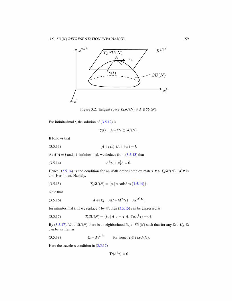
3.5. SU(N) REPRESENTATION INVARIANCE 159
x1
x2N2
R2N2
SU(N)
xk
ATASU(N)
τA
γ(t)
Figure 3.2: Tangent space TASU(N) at A ∈ SU(N).
For infinitesimal t, the solution of (3.5.12) is
γ(t) = A+ tτA ⊂ SU(N).
It follows that
(3.5.13) (A+ tτA)†(A+ tτA) = I.
As A†A = I and t is infinitesimal, we deduce from (3.5.13) that
(3.5.14) A†τA + τ†AA = 0.
Hence, (3.5.14) is the condition for an N-th order complex matrix τ ∈ TASU(N): A†τ is
anti-Hermitian. Namely,
(3.5.15) TASU(N) = τ | τ satisfies (3.5.14).
Note that
(3.5.16) A+ tτA = A(I+ tA†τA) = AetA†τA ,
for infinitesimal t. If we replace τ by iτ , then (3.5.15) can be expressed as
(3.5.17) TASU(N) = iτ | A†τ = τ†A, Tr(A†τ) = 0.
By (3.5.17), ∀A ∈ SU(N) there is a neighborhood UA ⊂ SU(N) such that for any Ω ∈ UA,Ωcan be written as
(3.5.18) Ω = AeiA†τ for some iτ ∈ TASU(N).
Here the traceless condition in (3.5.17)
Tr(A†τ) = 0
160 CHAPTER 3. MATHEMATICAL FOUNDATIONS
is derived by (2.2.51) and det Ω = 1 for Ω as in (3.5.18).
In particular, at the unit matrix e = I, we have
(3.5.19)TeSU(N) = iτ| τ† = τ, Trτ = 0,Ω = eiτ , τ ∈ TeSU(N),
where Ω ⊂ SU(N) is in a neighborhood of e = I.
3. Coordinate systems on TSU(N). Since the representation (3.5.17)-(3.5.18) of SU(N) is
essentially the same for all A ∈ SU(N), it suffices to only consider the representation (3.5.19)
of SU(N) at the unit matrix e = I.
It is known that TeSU(N) is an N2 − 1 dimensional linear space. Therefore we can take a
coordinate basis, called the generator basis of SU(N), denoted by
(3.5.20) τ1, · · · ,τK (K = N2 − 1),
such that for any τ ∈ TeSU(N), we have
(3.5.21) τ = θ aτa,
and θ a (1 ≤ a ≤ K) are complex numbers, called the coordinate system on TeSU(N). In this
case, Ω in (3.5.19) can be expressed as
Ω = eiθ aτa Ω ⊂ SU(N).
3.5.3 SU(N) tensors
Let (τ1, · · · ,τK) ⊂ TeSU(N) be a generator basis of SU(N). If the basis undergoes a linear
transformation:
(3.5.22)τa = xb
aτb,
X = (xba) is a complex K-th order matrix,
then the coordinate system (θ 1, · · · ,θ K) of TeSU(N) also undergoes a corresponding trans-
formation as follows
(3.5.23)θ a = ya
bθ b,
Y = (yab) is a complex K-th order matrix.
Since the expression (3.5.21) is independent of the choice of the generator bases of SU(N),we have
θ aτa = (θ 1, · · · ,θ K)Y T X
τ1
...
τK
= θ aτa,
which requires that
(3.5.24) Y = (X−1)T .
Thus, we see that (θ 1, · · · ,θ K) is a first order contra-variant tensor defined on TeSU(N).We are now ready to define more general SU(N) tensors.
3.5. SU(N) REPRESENTATION INVARIANCE 161
Definition 3.30 (SU(N) Tensors). Let T be given as
T = Ta1···ai
b1···b j| 1 ≤ ak,bl ≤ K = N2 − 1.
We say that T is a (i, j)-type of SU(N) tensor, under the generator basis transformation as
(3.5.22), we have
Ta1···ai
b1···b j= ya1
c1· · ·yai
cix
d1b1· · ·xd j
b jT
c1···ci
d1···d j,
where (xab) and (ya
b) are as in (3.5.22) and (3.5.23).
Based on Definition 3.30, it is easy to see that the SU(N) gauge fields (A1µ , · · · ,Aa
µ) is a
contra-variant SU(N) tensor. In other words, under (3.5.22), (A1µ , · · · ,Aa
µ) transforms as
(3.5.25) Aaµ = ya
bAbµ , Y = (ya
b) as in (3.5.24).
This can be seen from the fact that the operator Aaµτa in the differential operator Dµ in (3.5.4)
is independent of generator bases τa of SU(N).We now verify that the structure constants λ a
bc of SU(N) constitute a (1,2)-type of SU(N)tensor. By the definition of λ a
bc,
[τb,τc] = τbτ†c − τcτ†
b = iλ abcτa.
By (3.5.22),
[τb, τc] = xabxd
c [τa,τd ] = ixabxd
c λ fadτ f ,
and by definition
[τb, τc] = iλ abcτa = iλ a
bcxdaτd .
Then it follows that
(3.5.26) λ abc = x
fb xg
cyadλ d
f g,
which means that λ abc is a (1,2)-type SU(N) tensor.
Next, we introduce two second-order covariant SU(N) tensors Gab and gab, and later we
shall prove that they are equivalent.
Let A ∈ SU(N). Then the tangent space TASU(N) is given by (3.5.17). Let
(3.5.27) ω1, · · · ,ωK ∈ TASU(N),
be a generator basis of SU(N) at A.
1) SU(N) tensor Gab(A). By the basis (3.5.27) we can get a 2-covariant SU(N) tensor
defined by
(3.5.28) Gab(A) =1
2tr(ωaω†
b ), A ∈ SU(N),
where ωa (1 ≤ a ≤ K) are as in (3.5.27).
162 CHAPTER 3. MATHEMATICAL FOUNDATIONS
2) SU(N) tensor gab. The structure constants λ abc generated by the generators ωa in
(3.5.27) satisfy
(3.5.29) [ωb,ωc] = iλ abcωaA†, ∀A ∈ SU(N)
then we can define another 2-covariant tensor gab on TASU(N) by the structure con-
stants λ abc as follows
(3.5.30) gab =1
4Nλ c
adλ dcb.
The following theorem shows that both Gab and gab are symmetric second-order SU(N)tensors.
Theorem 3.31. The fields Gab(A) and gab given by (3.5.28) and (3.5.30) are 2-order sym-
metric SU(N) tensors, and for any A ∈ SU(N), the generator basis (3.5.27) satisfies (3.5.29),
where λ abc are the structure constants of SU(N) independent of A.
Proof. We first consider gab. By the anti-symmetry of the structure constants:
λ cab =−λ c
ba,
we deduce the symmetry of gab:
gab = λ cadλ d
cb = λ cdaλ d
bc = gba.
Now we verify the symmetry of Gab. By (3.5.17) the basis (ω1, · · · ,ωK) of TASU(N)satisfy that
(3.5.31) A†ωa = (A†ωa)†, tr(A†ωa) = 0, A† = A−1,
Namely A†ωa are Hermitian. Let A†ωa = τa, then
(3.5.32) τa = τ†a , trτa = 0.
Thus we have
(3.5.33) Gab =1
2tr(ωaω†
b ) =1
2tr(Aτaτ†
b A†) =1
2tr(τaτ†
b ).
Thanks to (3.5.32), (τ1, · · · ,τK) ∈ TeSU(N). Hence we have
(3.5.34) τaτ†b = τbτ†
a + iλ cabτc, trτc = 0.
It follows from (3.5.33) and (3.5.34) that
Gab =1
2tr(τaτ†
b ) =1
2tr(τbτ†
a ) = Gba.
Hence Gab is symmetry.
Finally we prove that for any A ∈ SU(N), each generator basis (ω1, · · · ,ωK) of TASU(N)satisfy (3.5.29). In fact, by (3.5.31), τa = A†ωa (1 ≤ a ≤ K) constitute a basis of TeSU(N).Therefore τa satisfies (3.5.34), i.e.
A†[ωa,ωb]A = iλ cabA†ωc.
Hence we obtain (3.5.29). The proof is complete.
3.5. SU(N) REPRESENTATION INVARIANCE 163
3.5.4 Intrinsic Riemannian metric on SU(N)
By Theorem 3.31, Gab(A) and gab are symmetric. We now show that both Gab and gab are
positive definite, and consequently Gab(A) is an intrinsic Riemannian metric on SU(N).
Theorem 3.32. For the 2-order SU(N) tensors gab and Gab, the following assertions hold
true:
1) The tensor gab given by (3.5.30) is positive definite; and
2) For each point A ∈ SU(N), there is a coordinate system in where Gab(A) = gab. There-
fore Gab(A) is a Riemannian metric on SU(N).
Proof. First, we prove Assertion (1). As a 2-order covariant tensor, gab transforms as
(3.5.35) (gab) = X(gab)XT , X = (xa
b) as in (3.5.22).
Hence, if for a given basis τa| 1 ≤ a ≤ K of TeSU(N) we can verify that gab =1
4Nλ c
adλ dcb
is positive definition, then by (3.5.35) we derive Assertion (1). In the following, we proceed
first for SU(2) and SU(3), then for the general SU(N).For SU(2), we take the Pauli matrices
(3.5.36) σ1 =
(0 1
1 0
), σ2 =
(0 −i
i 0
), σ3 =
(1 0
0 −1
)
as the generator basis of SU(2). The structure constants λ cab of (3.5.36) are as follows
(3.5.37) λ cab = 2εabc, εabc =
1 if (abc) is even,
− 1 if (abc) is odd,
0 if otherwise.
Based on (3.5.37), direct calculation shows that
gab =1
8λ c
adλ dcb = δab.
Namely (gab) = I is identity.
For SU(3), we can take the following Gell-Mann matrices as the generator basis of
SU(3):
λ1 =
0 1 0
1 0 0
0 0 0
, λ2 =
0 −i 0
i 0 0
0 0 0
, λ3 =
1 0 0
0 −1 0
0 0 0
,
λ4 =
0 0 1
0 0 0
−1 0 0
, λ5 =
0 0 −i
0 0 0
i 0 0
, λ6 =
0 0 0
0 0 1
0 1 0
,(3.5.38)
λ7 =
0 0 0
0 0 −i
0 i 0
, λ8 =
1√3
1 0 0
0 1 0
0 0 −2
.
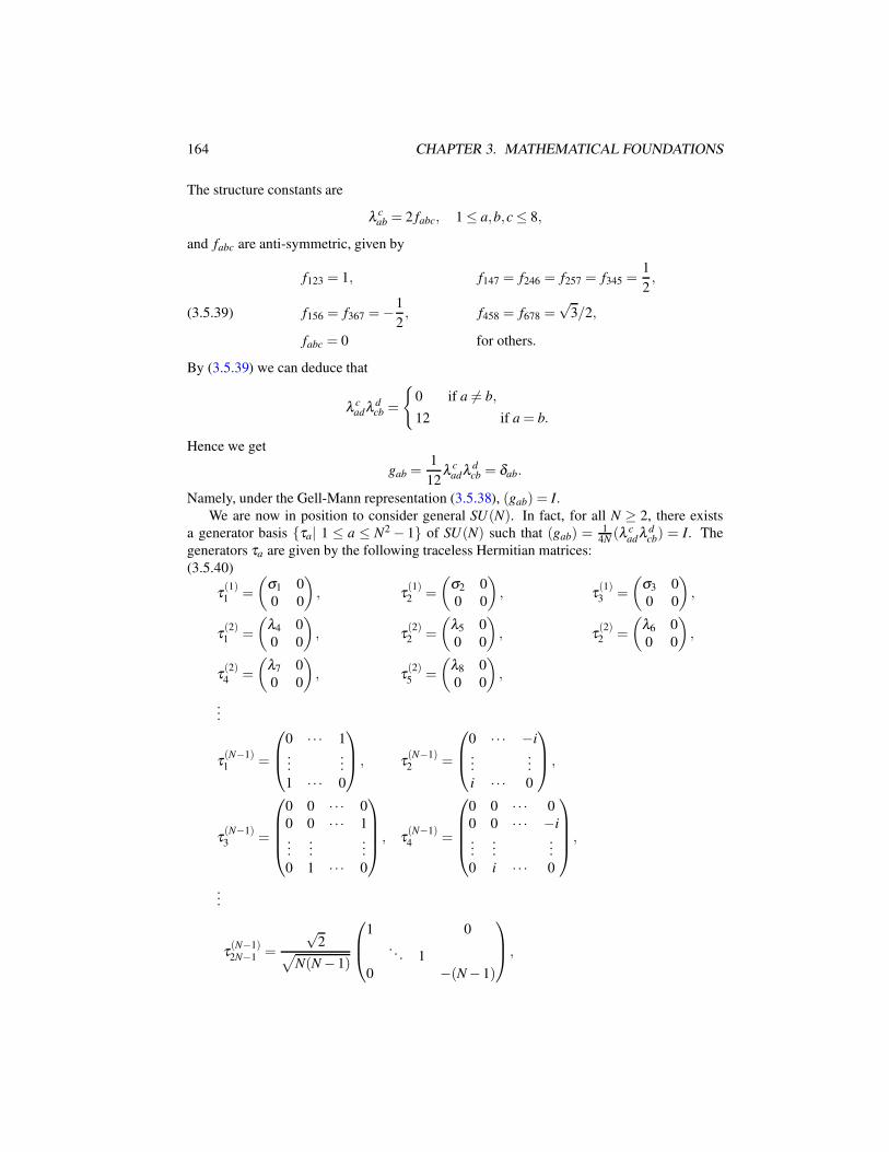
164 CHAPTER 3. MATHEMATICAL FOUNDATIONS
The structure constants are
λ cab = 2 fabc, 1 ≤ a,b,c ≤ 8,
and fabc are anti-symmetric, given by
f123 = 1, f147 = f246 = f257 = f345 =1
2,
f156 = f367 =−1
2, f458 = f678 =
√3/2,(3.5.39)
fabc = 0 for others.
By (3.5.39) we can deduce that
λ cadλ d
cb =
0 if a 6= b,
12 if a = b.
Hence we get
gab =1
12λ c
adλ dcb = δab.
Namely, under the Gell-Mann representation (3.5.38), (gab) = I.
We are now in position to consider general SU(N). In fact, for all N ≥ 2, there exists
a generator basis τa| 1 ≤ a ≤ N2 − 1 of SU(N) such that (gab) =1
4N(λ c
adλ dcb) = I. The
generators τa are given by the following traceless Hermitian matrices:
(3.5.40)
τ(1)1 =
(σ1 0
0 0
), τ
(1)2 =
(σ2 0
0 0
), τ
(1)3 =
(σ3 0
0 0
),
τ(2)1 =
(λ4 0
0 0
), τ
(2)2 =
(λ5 0
0 0
), τ
(2)2 =
(λ6 0
0 0
),
τ(2)4 =
(λ7 0
0 0
), τ
(2)5 =
(λ8 0
0 0
),
...
τ(N−1)1 =
0 · · · 1...
...
1 · · · 0
, τ
(N−1)2 =
0 · · · −i...
...
i · · · 0
,
τ(N−1)3 =
0 0 · · · 0
0 0 · · · 1...
......
0 1 · · · 0
, τ
(N−1)4 =
0 0 · · · 0
0 0 · · · −i...
......
0 i · · · 0
,
...
τ(N−1)2N−1 =
√2√
N(N − 1)
1 0
. . . 1
0 −(N − 1)
,
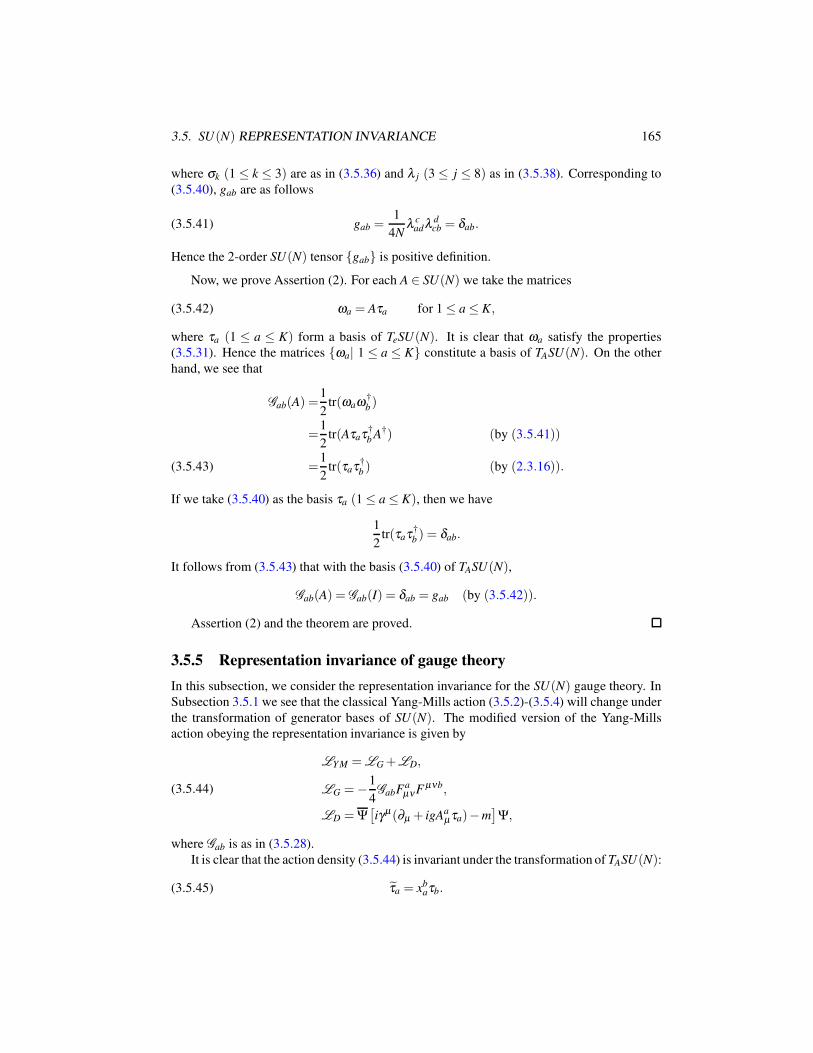
3.5. SU(N) REPRESENTATION INVARIANCE 165
where σk (1 ≤ k ≤ 3) are as in (3.5.36) and λ j (3 ≤ j ≤ 8) as in (3.5.38). Corresponding to
(3.5.40), gab are as follows
(3.5.41) gab =1
4Nλ c
adλ dcb = δab.
Hence the 2-order SU(N) tensor gab is positive definition.
Now, we prove Assertion (2). For each A ∈ SU(N) we take the matrices
(3.5.42) ωa = Aτa for 1 ≤ a ≤ K,
where τa (1 ≤ a ≤ K) form a basis of TeSU(N). It is clear that ωa satisfy the properties
(3.5.31). Hence the matrices ωa| 1 ≤ a ≤ K constitute a basis of TASU(N). On the other
hand, we see that
Gab(A) =1
2tr(ωaω†
b )
=1
2tr(Aτaτ†
b A†) (by (3.5.41))
=1
2tr(τaτ†
b ) (by (2.3.16)).(3.5.43)
If we take (3.5.40) as the basis τa (1 ≤ a ≤ K), then we have
1
2tr(τaτ†
b ) = δab.
It follows from (3.5.43) that with the basis (3.5.40) of TASU(N),
Gab(A) = Gab(I) = δab = gab (by (3.5.42)).
Assertion (2) and the theorem are proved.
3.5.5 Representation invariance of gauge theory
In this subsection, we consider the representation invariance for the SU(N) gauge theory. In
Subsection 3.5.1 we see that the classical Yang-Mills action (3.5.2)-(3.5.4) will change under
the transformation of generator bases of SU(N). The modified version of the Yang-Mills
action obeying the representation invariance is given by
(3.5.44)
LY M = LG +LD,
LG =−1
4GabFa
µνF µνb,
LD = Ψ[iγµ(∂µ + igAa
µτa)−m]
Ψ,
where Gab is as in (3.5.28).
It is clear that the action density (3.5.44) is invariant under the transformation of TASU(N):
(3.5.45) τa = xbaτb.
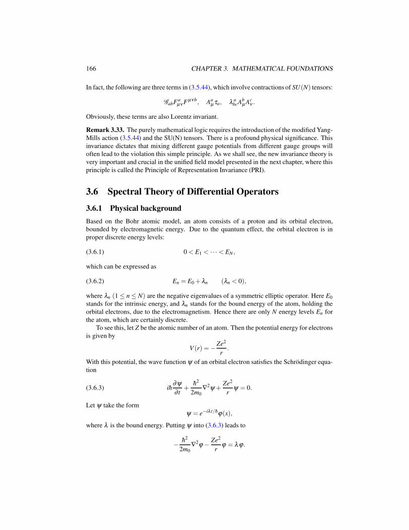
166 CHAPTER 3. MATHEMATICAL FOUNDATIONS
In fact, the following are three terms in (3.5.44), which involve contractions of SU(N) tensors:
GabFaµνFµνb, Aa
µτa, λ abcAb
µAcν .
Obviously, these terms are also Lorentz invariant.
Remark 3.33. The purely mathematical logic requires the introduction of the modified Yang-
Mills action (3.5.44) and the SU(N) tensors. There is a profound physical significance. This
invariance dictates that mixing different gauge potentials from different gauge groups will
often lead to the violation this simple principle. As we shall see, the new invariance theory is
very important and crucial in the unified field model presented in the next chapter, where this
principle is called the Principle of Representation Invariance (PRI).
3.6 Spectral Theory of Differential Operators
3.6.1 Physical background
Based on the Bohr atomic model, an atom consists of a proton and its orbital electron,
bounded by electromagnetic energy. Due to the quantum effect, the orbital electron is in
proper discrete energy levels:
(3.6.1) 0 < E1 < · · ·< EN ,
which can be expressed as
(3.6.2) En = E0 +λn (λn < 0),
where λn (1 ≤ n ≤ N) are the negative eigenvalues of a symmetric elliptic operator. Here E0
stands for the intrinsic energy, and λn stands for the bound energy of the atom, holding the
orbital electrons, due to the electromagnetism. Hence there are only N energy levels En for
the atom, which are certainly discrete.
To see this, let Z be the atomic number of an atom. Then the potential energy for electrons
is given by
V (r) =−Ze2
r.
With this potential, the wave function ψ of an orbital electron satisfies the Schrodinger equa-
tion
(3.6.3) ih∂ψ
∂ t+
h2
2m0
∇2ψ +Ze2
rψ = 0.
Let ψ take the form
ψ = e−iλ t/hϕ(x),
where λ is the bound energy. Putting ψ into (3.6.3) leads to
− h2
2m0
∇2ϕ − Ze2
rϕ = λ ϕ .
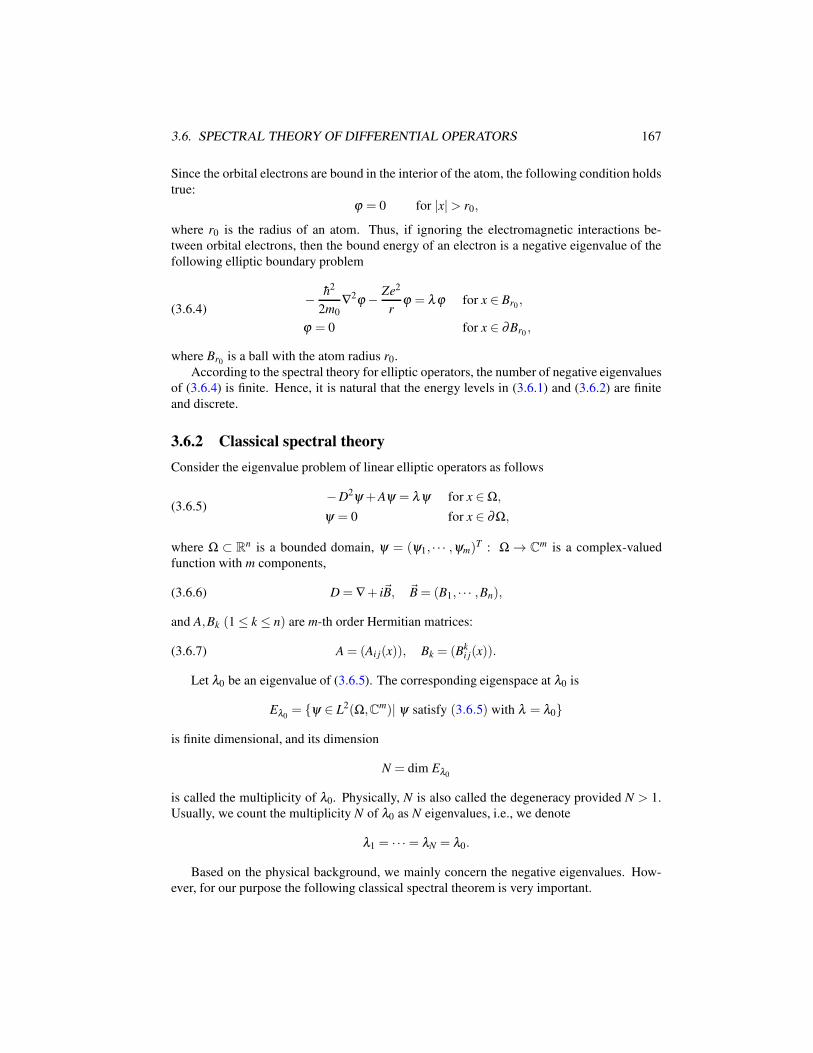
3.6. SPECTRAL THEORY OF DIFFERENTIAL OPERATORS 167
Since the orbital electrons are bound in the interior of the atom, the following condition holds
true:
ϕ = 0 for |x|> r0,
where r0 is the radius of an atom. Thus, if ignoring the electromagnetic interactions be-
tween orbital electrons, then the bound energy of an electron is a negative eigenvalue of the
following elliptic boundary problem
(3.6.4)− h2
2m0
∇2ϕ − Ze2
rϕ = λ ϕ for x ∈ Br0
,
ϕ = 0 for x ∈ ∂Br0,
where Br0is a ball with the atom radius r0.
According to the spectral theory for elliptic operators, the number of negative eigenvalues
of (3.6.4) is finite. Hence, it is natural that the energy levels in (3.6.1) and (3.6.2) are finite
and discrete.
3.6.2 Classical spectral theory
Consider the eigenvalue problem of linear elliptic operators as follows
(3.6.5)−D2ψ +Aψ = λ ψ for x ∈ Ω,
ψ = 0 for x ∈ ∂Ω,
where Ω ⊂ Rn is a bounded domain, ψ = (ψ1, · · · ,ψm)T : Ω → Cm is a complex-valued
function with m components,
(3.6.6) D = ∇+ i~B, ~B = (B1, · · · ,Bn),
and A,Bk (1 ≤ k ≤ n) are m-th order Hermitian matrices:
(3.6.7) A = (Ai j(x)), Bk = (Bki j(x)).
Let λ0 be an eigenvalue of (3.6.5). The corresponding eigenspace at λ0 is
Eλ0= ψ ∈ L2(Ω,Cm)| ψ satisfy (3.6.5) with λ = λ0
is finite dimensional, and its dimension
N = dim Eλ0
is called the multiplicity of λ0. Physically, N is also called the degeneracy provided N > 1.
Usually, we count the multiplicity N of λ0 as N eigenvalues, i.e., we denote
λ1 = · · ·= λN = λ0.
Based on the physical background, we mainly concern the negative eigenvalues. How-
ever, for our purpose the following classical spectral theorem is very important.
168 CHAPTER 3. MATHEMATICAL FOUNDATIONS
Theorem 3.34 (Spectral Theorem of Elliptic Operators). Let the matrices in (3.6.7) are Her-
mitian, and the functions Ai j,Bki j ∈ L∞(Ω). The the following assertions hold true:
1) All eigenvalues of (3.6.5) are real with finite multiplicities, and form an infinite conse-
quence as follows:
−∞ < λ1 ≤ λ2 ≤ ·· · ≤ λk ≤ ·· · , λk → ∞ as k → ∞.
where λk is counting the multiplicity.
2) The eigenfunctions ψk corresponding to λk are orthogonal to each other, i.e.
∫
Ωψ†
k ψ jdx = 0 ∀k 6= j.
In particular, ψk is an orthogonal basis of L2(Ω,Cm).
3) There are only finite number of negative eigenvalues in λk,
(3.6.8) −∞ < λ1 ≤ ·· · ≤ λN < 0,
and the number N of negative eigenvalues depends on the matrices A,B j in (3.6.7) and
the domain Ω.
Remark 3.35. For the energy levels of subatomic particles introduced in Chapter 5, we are
mainly interested in the negative eigenvalues of (3.6.5) and in the estimates of the number N
in (3.6.8).
Theorem 3.34 is a corollary of the classical Lagrange multiplier theorem. We recall the
variational principle with constraint. Let H be a linear normed space, and F and G are two
functionals on H:
F,G : H →R1.
Let Γ ⊂ H be the set
Γ = u ∈ H| G(u) = 1.
If u0 ∈ Γ is a minimum point of F with constraint on Γ:
F(u0) = minu∈Γ
F(u),
then u0 satisfies the equation
(3.6.9) δF(u0) = λ δG(u0),
where λ is a real number.
For the eigenvalue equation of (3.6.5), the corresponding functional is
(3.6.10) F(ψ) =
∫
Ω
[|Dψ |2 +ψ†Aψ
]dx,
3.6. SPECTRAL THEORY OF DIFFERENTIAL OPERATORS 169
and the constraint functional G is given by
(3.6.11) G(ψ) =
∫
Ω|ψ |2dx.
It is easy to see that the equation of (3.6.5) is of the form:
δF(ψ) = λ δG(ψ),
and F,G are as in (3.6.10) and (3.6.11), which is as the variational equation (3.6.9) with the
constraint on Γ.
Hence, the eigenvalues λk (k = 1,2, · · ·) of (3.6.5) can be expressed in the following forms
(3.6.12)
λ1 = minψ∈Γ
F(ψ),
λk = minψ∈Γ,ψ∈H⊥
k−1
F(ψ),
where F is as in (3.6.10), Γ and H⊥k−1 are the sets:
(3.6.13)
Γ = ψ ∈ H10 (Ω,Cm)| ||ψ ||L2 = 1,
H⊥k−1 =
ψ ∈ H1
0 (Ω,Cm)∣∣∣∫
Ωψ†ψ jdx = 0, 1 ≤ j ≤ k− 1
,
and ψ j (1 ≤ j ≤ k− 1) are the eigenfunctions corresponding to the first (k− 1) eigenvalues
λ1, · · · ,λk−1. Namely H⊥k−1 is the orthogonal complement of Hk−1 = spanψ1, · · · ,ψk−1 in
H10 (Ω,Cm).
Based on (3.6.12)-(3.6.13), we readily deduce the spectral theorem, Theorem 3.34, for
the elliptic eigenvalue problem (3.6.5).
3.6.3 Negative eigenvalues of elliptic operators
The following theorem provides a necessary and sufficient condition for the existence of
negative eigenvalues of (3.6.5), and a criterion to estimate the number of negative eigenvalues.
Theorem 3.36. For the eigenvalue problem (3.6.5), the following assertions hold true:
1) Equations (3.6.5) have negative eigenvalues if and only if there is a function ψ ∈H1
0 (Ω,Cm), such that
(3.6.14)
∫
Ω[(Dψ)†(Dψ)+ψ†Aψ ]dx < 0,
where D is as in (3.6.6).
2) If there are K linear independent functions ψ1, · · · ,ψK ∈ H10 (Ω,Cm), such that
(3.6.15) ψ satisfies (3.6.14) for any ψ ∈ EK = span ψ1, · · · ,ψK,
then the number N of negative eigenvalues is larger than K, i.e., N ≥ K.
170 CHAPTER 3. MATHEMATICAL FOUNDATIONS
Proof. Assertion (1) follows directly from the following classical formula for the first eigen-
value λ1 of (3.6.5):
λ1 = minψ∈H1
0 (Ω,Cm)
1
||ψ ||L2
∫
Ω
[(Dψ)†(Dψ)+ψ†Aψ
]dx.
We now prove Assertion (2) by contradiction. Assume that it is not true, then K > N. By
Theorem 3.34, the K functions ψ j in (3.6.15) can be expended as
(3.6.16) ψ j =N
∑i=1
α jiei +∞
∑l=1
β jlϕl for 1 ≤ j ≤ K,
where ei (1 ≤ i ≤ N) and ϕl are eigenfunctions corresponding to negative and nonnegative
eigenvalues. Since K > N, there exists a K-th order matrix P such that
(3.6.17) Pα =
(0 · · · 0
∗
),
where
α =
α11 · · · α1N
......
αK1 · · · αKN
with αi j as in (3.6.16).
Thus, under the transformation P,
(3.6.18) ψ = P
(ψ
0
)∈ EK , ψ = (ψ1, · · · ,ψN)
T ,
where EK is as in (3.6.15).
However, by (3.6.14) and (3.6.15), the first term ψ1 in (3.6.18) can be expressed in the
form
(3.6.19) ψ1 =∞
∑l=1
θlϕl ∈ EK .
Note that ϕl are the eigenfunctions corresponding to the nonnegative eigenvalues of (3.6.5).
Hence we have
∫
Ω[(Dψ1)
†(Dψ1)+ ψ†1 Aψ1]dx =
∫
Ωψ†
1 (−D2ψ1 +Aψ1)dx =∞
∑l=1
|θl |2λl > 0.(3.6.20)
Here λl ≥ 0 are the nonnegative eigenvalues of (3.6.5). Hence we derive, from (3.6.19) and
(3.6.20), a contradiction with the assumption in Assertion (2). The proof of the theorem is
complete.
3.6. SPECTRAL THEORY OF DIFFERENTIAL OPERATORS 171
3.6.4 Estimates for number of negative eigenvalues
For simplicity, it is physically sufficient for us to consider the eigenvalue problem of the
Laplace operators, given by
(3.6.21)−∇2ψ +V(x)ψ = λ ψ for x ∈ Br,
ψ = 0 for x ∈ ∂Br,
where Br ⊂ Rn is a ball with radius r.
In physics, V represents a potential function and takes negative value in a bound state,
ensuring by Theorem 3.36 that (3.6.21) possesses negative eigenvalues.
Here, for the potential function V (x), we assume that
(3.6.22) V (ρx)≃ ραV0(x) (α >−2),
where V0(x) is defined in the unit ball B1, and
(3.6.23) Ω = x ∈ B1 | V0(x)< 0 6= /0.
Let θ > 0 be defined by
(3.6.24) θ = infψ∈L2(Ω,Cm)
1
||ψ ||L2
∫
Ω|V (x)| |ψ |2dx.
The main result in this section is the following theorem, which provides a relation be-
tween N,θ and r, where N is the number of negative eigenvalues of (3.6.21). Let λ1 be the
first eigenvalue of the equation
(3.6.25)−∆e = λ e for x ∈ Ω,
e = 0 for x ∈ ∂Ω,
where Ω ⊂ B1 is as defined by (3.6.23).
To state the main theorem, we need to introduce a lemma, leading to the Weyl asymptotic
relation (Weyl, 1912).
Lemma 3.37 (H. Weyl). Let λN be the N-th eigenvalue of the m-th order elliptic operator
(3.6.26)(−1)m∆me = λ e for x ∈ Ω ⊂ R
n,
Dke|∂Ω = 0 for 0 ≤ k ≤ m− 1,
then λN has the asymptotical relation
(3.6.27) λN ∼ λ1N2m/n,
where λ1 is the first eigenvalue of (3.6.26).
We are now ready for the main theorem.
172 CHAPTER 3. MATHEMATICAL FOUNDATIONS
Theorem 3.38. Under the assumptions of (3.6.22) and (3.6.23), the number N of the negative
eigenvalues of (3.6.21) satisfies the following approximative relation
(3.6.28) N ≃(
θ r2+α
λ1
)n/2
,
provided that θ r2+α/λ1 ≫ 1 is sufficiently large, where r and θ are as in (3.6.21) and
(3.6.24), and λ1 is the first eigenvalue of (3.6.25).
Proof. The ball Br can be written as
Br = y = rx | x ∈ B1.
Note that ∂/∂y = r−1∂/∂x, (3.6.21) can be equivalently expressed as
(3.6.29)−∆ϕ + r2V (rx)ϕ = β ϕ for x ∈ B1,
ϕ = 0 for x ∈ ∂B1,
and the eigenvalue λ of (3.6.21) is
λ =1
r2β , where β is the eigenvalue of (3.6.29).
Hence the number of negative eigenvalues of (3.6.21) is the same as that of (3.6.29), and we
only need to prove (3.6.28) for (3.6.29).
By (3.6.22), the equation (3.6.29) is approximatively in the form
(3.6.30)−∆ϕ + r2+αV0(x)ϕ = β ϕ for x ∈ B1,
ϕ = 0 for x ∈ ∂B1.
Based on Assertion (2) in Theorem 3.36, we need to find N linear independent functions
ϕn ∈ H10 (B1) (1 ≤ n ≤ N) satisfying
(3.6.31)
∫
B1
[|∇ϕ |2 + r2+αV0(x)ϕ
2]
dx < 0,
for any ϕ ∈ span ϕ1, · · · ,ϕN with ||ϕ ||L2 = 1.
To this end, we take the eigenvalues λn and eigenfunctions en of (3.6.25) such that
0 < λ1 ≤ ·· · ≤ λN < λN+1,
and
(3.6.32) λN < θ r2+α ≤ λN+1.
For the eigenfunctions en, we make the extension
ϕn =
en for x ∈ Ω,
0 for x ∈ B1/Ω.
3.6. SPECTRAL THEORY OF DIFFERENTIAL OPERATORS 173
It is known that ϕn is weakly differentiable, and ϕn ∈ H10 (Ω). These functions ϕn (1≤ n ≤N)
are what we need. Let
ϕ =N
∑n=1
αnϕn, ||ϕ ||L2 = 1.
By Assertion (2) in Theorem 3.36, ϕn (1 ≤ n ≤ N) are orthonormal:
∫
B1
ϕiϕ jdx =∫
Ωeie jdx = δi j.
Therefore we have
(3.6.33) ||ϕ ||L2 =N
∑n=1
α2n = 1.
Thus the integral in (3.6.31) is
∫
B1
[|∇ϕ |2 + r2+αV0(x)ϕ2]dx =
∫
Ω−(
N
∑n=1
αnen
)(N
∑n=1
αn∆en
)dx+ r2+α
∫
ΩV0(x)ϕ
2dx
=N
∑n=1
α2n λn + r2+α
∫
ΩV0(x)ϕ
2dx
≤N
∑n=1
α2n λn −θ r2+α by (3.6.24)
< 0 by (3.6.32) and (3.6.33).
It follows from Theorem 3.36 that there are at least N negative eigenvalues for (3.6.30). When
θ r2+α ≫ 1 is sufficiently large, the relation (3.6.32) implies that
(3.6.34) λN ≃ θ r2+α .
On the other hand, by (3.6.27) in Lemma 3.37,
(3.6.35) λN ∼ λ1N2/n (m = 1).
Hence the relation (3.6.28) follows from (3.6.34) and (3.6.35). The proof is complete.
Remark 3.39. In Section 6.4.6, we shall see that for particles with mass m, the parameters
in (3.6.28) are
α = 0, r = 1, n = 3, θ = 4mρ21 Ag2/h2ρ ,
where g = gw or gs is the weak or strong interaction charge, ρ is the particle radius, ρ1 is the
weak or strong attracting radius, and A is the weak or strong interaction constant. Hence the
number of energy levels of massive particles is given by
N =
[4
λ1
ρ21 A
ρ
mc
h
g2
hc
]3/2
.
where λ1 is the first eigenvalue of −∆ in the unit ball B1.
174 CHAPTER 3. MATHEMATICAL FOUNDATIONS
Example 3.40 (Number of Atomic Energy Levels). As an application of Theorem 3.38, we
consider here the estimates for the number of atomic energy levels. Let the atom number be
Z. If ignoring interactions between orbital electrons, then the spectral equation is as follows
−∆ψ +V(x)ψ = λ ψ for x ∈ Br0,
ψ = 0 for x ∈ ∂Br0,
and r0 is the atom radius, V is the potential energy, given by
V (x) =−2Zme2
h2
1
r, m the mass of electron.
The parameters in (3.6.28) for this system are
(3.6.36) α =−1, n = 3, r = r0 = 10−8cm.
In addition, V0 and Ω in (3.6.23) and (3.6.24) are as
V0 =−2Zme2
h2, Ω = B1.
Therefore, the parameter θ is given by
(3.6.37) θ =2Zme2
h2.
According to physical parameters, it is known that
(3.6.38) r0 ×mc
h=
1
4× 10³,
e2
hc=
1
137.
Hence, by (3.6.36)-(3.6.38) the formulas (3.6.28) becomes
(3.6.39) N =
(2Z
λ1
e2
hc
mcr0
h
)3/2
=
(103Z
274λ1
)3/2
,
where λ1 is the first eigenvalue of −δ on B1.
The formulas is derived in the ideal situation ignoring interactions between orbital elec-
trons, and only holds for a bigger atom number Z.
3.6.5 Spectrum of Weyl operators
In Section 6.4.2, we shall deduce from Basic Postulates of Quantum Mechanics that the
spectral equations for the massless subatomic particles are in the following form
(3.6.40)− hc(~σ ·~D)2ϕ +
ig
2(~σ ·~D),A0ϕ = iλ (~σ ·~D)ϕ ,
ϕ |∂Ω = 0,
3.6. SPECTRAL THEORY OF DIFFERENTIAL OPERATORS 175
where ϕ = (ϕ1,ϕ2)T : Ω → C2 is a complex-valued function with two components, called
the Weyl spinor, ~σ = (σ1,σ2,σ2) is the Pauli matrix operator as given by (3.5.36), ~D =(D1,D2,D3) is the derivative operator given by
(3.6.41) Dk = ∂k + igAk for k = 1,2,3,
and (~σ ·~D),A0 is the anti-commutator defined by
(~σ ·~D),A0= (~σ ·~D)A0 +A0(~σ ·~D).
Remark 3.41. The equation (3.6.40) is essentially an eigenvalue problem of the first order
differential operator:
ihc(~σ ·~D)+ gA0,
which is called the Weyl operator. In addition, the operator (~σ ·~D)2 in (3.6.40) is elliptic and
can be written as
(3.6.42) (~σ ·~D)2 = D2 − g
hc~σ · curl~A,
and ~A= (A1,A2,A3) as in (3.6.41). The ellipticity of (3.6.42) g in (3.6.41)-(3.6.42) represents
the weak or strong interaction charge, and Aµ =(A0,A1,A2,A3) the weak or strong interaction
potential.
Note also that ~A = (A1,A2,A3) stands for the magnetic component of the weak or strong
interaction. Hence, in (3.6.42), the term
g~σ · curl~A
represents magnetic energy generated by the weak or strong interactions, which is an impor-
tant byproduct of the unified field theory based on PID and PRI.
Since (3.6.40) is essentially an eigenvalue problem of first-order differential equations,
its negative and positive eigenvalues are infinite. However, if we only consider the physically
meaningful eigenstates, then the number of negative eigenvalues of (3.6.40) is finite. We now
give introduce these physical meaningful eigenvalues and eigenfunctions for (3.6.40).
Definition 3.42. A real number λ and a two-component wave function ϕ ∈ H10 (Ω,C2) are
called the eigenvalue and eigenfunction of (3.6.40), if (λ ,ϕ) satisfies (3.6.40) and
(3.6.43)
∫
Ωϕ†[i(~σ ·~D)ϕ
]dx > 0.
The physical significance of (3.6.43) is that the kinetic energy E of the eigenstate ϕ is
positive: E > 0.
The following theorem ensures the mathematical rationality of the eigenvalue problem of
the Weyl operators.
Theorem 3.43 (Spectral Theorem of Weyl Operators). For the eigenvalue problem (3.6.40),
the following assertions hold true:
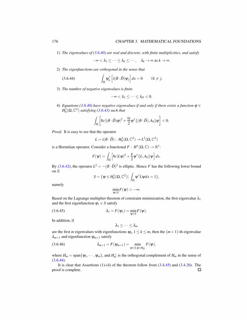
176 CHAPTER 3. MATHEMATICAL FOUNDATIONS
1) The eigenvalues of (3.6.40) are real and discrete, with finite multiplicities, and satisfy
−∞ < λ1 ≤ ·· · ≤ λk ≤ ·· · , λk → ∞ as k → ∞.
2) The eigenfunctions are orthogonal in the sense that
(3.6.44)
∫
Ωψ†
k
[i(~σ ·~D)ψ j
]dx = 0 ∀k 6= j.
3) The number of negative eigenvalues is finite
−∞ < λ1 ≤ ·· · ≤ λN < 0.
4) Equations (3.6.40) have negative eigenvalues if and only if there exists a function ϕ ∈H1
0 (Ω,C2) satisfying (3.6.43) such that
∫
Ω
[hc|(~σ ·~D)ϕ |2 + ig
2ϕ†(~σ ·~D),A0ϕ
]< 0.
Proof. It is easy to see that the operator
L = i(~σ ·~D) : H10 (Ω,C2)→ L2(Ω,C2)
is a Hermitian operator. Consider a functional F : H1(Ω,C)→R1:
F(ψ) =
∫
Ω
[hc|Lψ |2 + g
2ψ†L,A0ψ
]dx.
By (3.6.42), the operator L2 = −(~σ ·~D)2 is elliptic. Hence F has the following lower bound
on S:
S = ψ ∈ H10 (Ω,C2)|
∫
Ωψ†Lψdx = 1,
namely
minψ∈S
F(ψ)>−∞.
Based on the Lagrange multiplier theorem of constraint minimization, the first eigenvalue λ1
and the first eigenfunction ϕ1 ∈ S satisfy
(3.6.45) λ1 = F(ψ1) = minψ∈S
F(ψ).
In addition, if
λ1 ≤ ·· · ≤ λm
are the first m eigenvalues with eigenfunctions ψk,1 ≤ k ≤ m, then the (m+1)-th eigenvalue
λm+1 and eigenfunction ψm+1 satisfy
(3.6.46) λm+1 = F(ψm+1) = minψ∈S,ψ∈H⊥
m
F(ψ),
where Hm = spanψ1, · · · ,ψm, and H⊥m is the orthogonal complement of Hm in the sense of
(3.6.44).
It is clear that Assertions (1)-(4) of the theorem follow from (3.4.45) and (3.4.26). The
proof is complete.
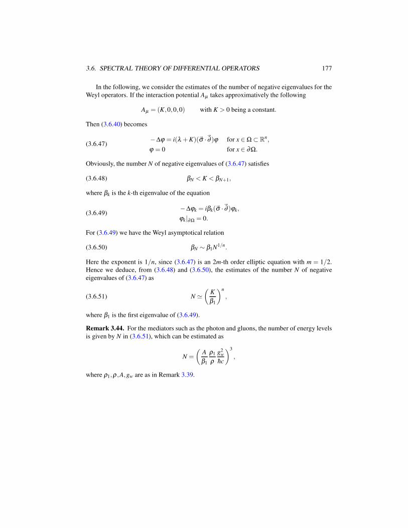
3.6. SPECTRAL THEORY OF DIFFERENTIAL OPERATORS 177
In the following, we consider the estimates of the number of negative eigenvalues for the
Weyl operators. If the interaction potential Aµ takes approximatively the following
Aµ = (K,0,0,0) with K > 0 being a constant.
Then (3.6.40) becomes
(3.6.47)−∆ϕ = i(λ +K)(~σ ·~∂ )ϕ for x ∈ Ω ⊂ R
n,
ϕ = 0 for x ∈ ∂Ω.
Obviously, the number N of negative eigenvalues of (3.6.47) satisfies
(3.6.48) βN < K < βN+1,
where βk is the k-th eigenvalue of the equation
(3.6.49)−∆ϕk = iβk(~σ ·~∂ )ϕk,
ϕk|∂Ω = 0.
For (3.6.49) we have the Weyl asymptotical relation
(3.6.50) βN ∼ β1N1/n.
Here the exponent is 1/n, since (3.6.47) is an 2m-th order elliptic equation with m = 1/2.
Hence we deduce, from (3.6.48) and (3.6.50), the estimates of the number N of negative
eigenvalues of (3.6.47) as
(3.6.51) N ≃(
K
β1
)n
,
where β1 is the first eigenvalue of (3.6.49).
Remark 3.44. For the mediators such as the photon and gluons, the number of energy levels
is given by N in (3.6.51), which can be estimated as
N =
(A
β1
ρ1
ρ
g2w
hc
)3
,
where ρ1,ρ ,A,gw are as in Remark 3.39.

178 CHAPTER 3. MATHEMATICAL FOUNDATIONS
Chapter 4
Unified Field Theory of Four
Fundamental Interactions
Once again, the goal of this book is to derive experimentally verifiable laws of Nature based
on a few fundamental mathematical principles. The aims of this chapter are are as follows:
• to address the basic principles for the unified field theory coupling the four fundamental
interactions,
• to derive the unified model based on these principles, and
• to study the mechanism and nature of individual interactions.
This chapter is based entirely on the recent work of the authors (Ma and Wang, 2015a,
2014h,c, 2013a, 2014e). The key ingredients of the unified field theory include the following.
First, we have established two new principles, the principle of interaction dynamics (PID)
and the principle of representation invariance (PRI). PID was first discovered by (Ma and Wang,
2014e, 2015a). It requires that for the four fundamental interactions, the variation be taken
under the energy-momentum conservation constraints. The validity of PID for the four fun-
damental interactions of Nature has been demonstrated through strong experimental and ob-
servation supports. For gravity, PID is induced by the presence of the dark matter and dark
energy phenomena. PID is also required by the Higgs field and the quark confinement, as we
explained in Chapter 1.
PRI, originally discovered by (Ma and Wang, 2014h), states that the SU(N) gauge theory
should be invariant, under the representation transformations of the generator bases. PRI is
simply a logic requirement for the SU(N) theory.
Second, with PRI, the unification through a large symmetry group appears to be not fea-
sible. Then we have demonstrated that the two first principles, PID and PRI, together with
the principle of symmetry-breaking, offer an entirely different route for the unification:
1) the general relativity and the gauge symmetries dictate the Lagrangian;
and
179
180 CHAPTER 4. UNIFIED FIELD THEORY
2) the coupling of the four interactions is achieved through PID and PRI in
the unified field equations, which obey the PGR and PRI, but break sponta-
neously the gauge symmetry.
In this chapter, there are four sections. Section 4.1 presents the general view of the uni-
fied field theory, the geometry of unified fields, gauge-symmetry breaking, PID, and PRI.
Section 4.2 presents the experimental and observational physical supports for PID. The math-
ematical reason from the well-posedness point of view is also given. Section 4.3 introduces
the unified field equations coupling the four fundamental interactions based on PID. Sec-
tion 4.4 presents the natural duality between the gauge fields and their dual fields, as well as
the decoupling of the unified field equations to the field equations for individual interaction
when the other interactions are negligible.
4.1 Principles of Unified Field Theory
4.1.1 Four interactions and their interaction mechanism
The four fundamental interactions/forces of Nature include
1) the gravitational force, generated by the mass charge M, which is responsible to all
macroscopic motions,
2) the electromagnetic force, generated by the electric charge e, which holds the atoms
and molecules together,
3) the strong force, generated by the strong charge gs, which mainly acts at three levels:
quarks and gluons, hadrons, and nucleons, and
4) the weak force, generated by the weak charge gw, which provides the binding energy
to hold the mediators, the leptons and quarks together.
The most crucial ingredient of each interaction is its corresponding interaction potential
Φ and charge g. The relation between the corresponding force F , its associated potential Φand its charge g is as follows:
(4.1.1) F =−g∇Φ,
where ∇ is the three-dimensional spatial gradient operator. The charge g for each interaction
is given as follows:
(4.1.2)
m the mass charge for gravity,
e the electric charge for electromagnetism,
gs the strong charge for strong interaction, and
gw the weak charge for the weak interaction.
4.1. PRINCIPLES OF UNIFIED FIELD THEORY 181
We know now that the four interactions are dictated respectively by the following sym-
metry principles:
(4.1.3)
gravity: principle of general relativity,
electromagnetism: U(1) gauge invariance,
weak interaction: SU(2) gauge invariance,
strong interaction: SU(3) gauge invariance.
The last three interactions also obey the Lorentz invariance. As a natural consequence, the
three charges e,gw,gs in (4.1.2) are the coupling constants of the U(1),SU(2),SU(3) gauge
fields.
Following the simplicity principle of laws of Nature as stated in Principle 2.2, the three ba-
sic symmetries—the Einstein general relativity, the Lorentz invariance and the gauge invariance—
uniquely determine the interaction fields and their Lagrangian actions for the four interac-
tions:
1. Gravity. The gravitational fields are the Riemannian metric defined on the space-time
manifold M :
(4.1.4) ds2 = gµνdxµdxν ,
and then second-order tensor gµν stands for the gravitational potential. The Lagrangian
action for the metric (4.1.4) is the Einstein-Hilbert functional
(4.1.5) LEH = R+8πG
c4S,
where R stands for the scalar curvature of the tangent bundle TM of M .
2. Electromagnetism. The field describing electromagnetic interaction is the U(1) gauge
field
Aµ = (A0,A1,A2,A3),
representing the electromagnetic potential, and the Lagrangian action is
(4.1.6) LEM =−1
4AµνAµν ,
which stands for the scalar curvature of the vector bundle M ⊗p C4, with
Aµν = ∂µAν − ∂νAµ .
being the curvature tensor.
3. Weak interaction. The weak fields are the SU(2) gauge fields
W aµ = (W a
0 ,Wa1 ,W
a2 ,W
a3 ) for 1 ≤ a ≤ 3,
and their action is
(4.1.7) LW =−1
4G
wabW a
µνW µνb,
182 CHAPTER 4. UNIFIED FIELD THEORY
which also stands for the scalar curvature of the spinor bundle: M ⊗p (C4)2. Here
W aµν = ∂µW a
ν − ∂νW aµ + gwλ a
bcWbµW c
ν for 1 ≤ a ≤ 3.
4. Strong interaction. The strong fields are the SU(3) gauge fields
Skµ = (Sk
0,Sk1,S
k2,S
k3) for 1 ≤ k ≤ 8,
and the action is
(4.1.8) LS =−1
4G
sklS
kµνSµνl ,
which corresponds to the scalar curvature of M ⊗p (C4)3. Here
Skµν = ∂µSk
ν − ∂νSkµ + gsΛ
krlS
rµSl
ν for 1 ≤ k ≤ 8.
The Yukawa Interaction Mechanism, briefly mentioned in Section 2.1.6 and restated be-
low, is the main reason why the weak interaction is described by an SU(2) gauge theory and
the strong interaction is described by an SU(3) gauge theory.
One great vision of Albert Einstein is his principle of equivalence, which says that gravity
is manifested as the curved effect of the space-time manifold M ,gµν. Based on the recent
work by the authors (Ma and Wang, 2015a, 2014h,d), the Einstein vision leads us to postulate
the Geometric Interaction Mechanism 2.13, which is restated here for convenience:
Geometric Interaction Mechanism 4.1. The gravitational force is the curved effect of the
time-space, and the electromagnetic, weak, strong interactions are the twisted effects of the
underlying complex vector bundles M ⊗p Cn.
Yukawa’s viewpoint, entirely different from Einstein’s, is that the other three fundamen-
tal forces—the electromagnetism, the weak and the strong interactions–take place through
exchanging intermediate bosons:
Yukawa Interaction Mechanism 4.2. The four fundamental interactions of Nature are me-
diated by exchanging interaction field particles, called the mediators. The gravitational force
is mediated by the graviton, the electromagnetic force is mediated by the photon, the strong
interaction is mediated by the gluons, and the weak interaction is mediated by the intermedi-
ate vector bosons W± and Z.
It is the Yukawa mechanism that leads to the SU(2) and SU(3) gauge theories respectively
for the weak and the strong interactions. In fact, the three mediators W± and Z for the weak
interaction are regarded as the SU(2) gauge fields W aµ (1 ≤ a ≤ 3), and the eight gluons for
the strong interaction are considered as the SU(3) gauge fields Skµ (1 ≤ k ≤ 8). Of course,
the three color quantum numbers for the quarks are an important evidence for choosing the
SU(3) gauge theory to describe the strong interaction.
The two interaction mechanisms lead to two entirely different directions to develop the
unified field theory. The need for quantization for all current theories for the four interactions
is based on the Yukawa Interaction Mechanism. The new unified field theory in this article is
4.1. PRINCIPLES OF UNIFIED FIELD THEORY 183
based on the Geometric Interaction Mechanism, which focuses directly on the four interaction
forces as in (4.1.1), and does not involve a quantization process.
A radical difference for these two mechanisms is that the Yukawa Mechanism is oriented
toward to computing the transition probability for the particle decays and scatterings, and the
Geometric Interaction Mechanism is oriented toward to fundamental laws, such as interaction
potentials, of the four interactions.
4.1.2 General introduction to unified field theory
Einstein’s unification
The aim of a unified field theory is to establish a set of field equations coupling the four
fundamental interactions. Albert Einstein was the first person who attempted to establish a
unified field theory. The basic philosophy of his unification is that all fundamental forces of
Nature should be dictated by one large symmetry group, which can degenerate into a sub-
symmetry for each interaction:
(4.1.9) Unification through an action under a large symmetry
In essence, with the Einstein unification, under the large symmetry, the four fundamental
forces can be regarded as one fundamental force.
Recall that there are four fundamental interactions of Nature: gravitational, electromag-
netic, strong, and weak, whose fields and actions:
1) fields gµν , Aµ , W aµ | 1 ≤ a ≤ 3 and Sk
µ | 1 ≤ k ≤ 8, and
2) their actions LEH , LEM, LW and LS,
are dictated by the symmetries in (4.1.3), as described in (4.1.5)-(4.1.8).
Basically, the Einstein unification is to search for a large symmetry, which dictates an N
component field G:
(4.1.10) G = (G1, · · · ,GN),
and an action
(4.1.11) L = L (G1, · · · ,GN).
The basic requirements for such a unification are as follows: Under certain conditions,
1) the large symmetry degenerates into sub-symmetries: the general invariance, the Lorentz
invariance, and the U(1),SU(2),SU(3) invariance;
2) the field G of (4.1.10) is then decomposed into the fields of the four fundamental inter-
actions:
(4.1.12) (G1, · · · ,GN)degenerate−→ gµν ,Aµ ,W
aµ ,S
kµ ,
184 CHAPTER 4. UNIFIED FIELD THEORY
3) the action (4.1.11) also becomes the simple sum of these actions given in (4.1.5)-
(4.1.8):
(4.1.13) L (G1, · · · ,GN)→ LEH +LEM +LW +LS.
For almost a century, a great deal of effort has been made to find the unified field model
based on the above mentioned approach. However, all efforts in this aspect are not successful.
In fact, among other reasons, this route of unification violates the principle of representation
invariance (PRI), discovered in (Ma and Wang, 2014h); see also remaining part of this chapter
for details.
Moreover, the basic principles and the field equations from all attempted unified field the-
ories based on (4.1.9) are often too complex, and violate the simplicity principle of physics.
Most importantly, despite of many attempts, the current theories following (4.1.9) fail to
provide solutions to the following longstanding problems and challenges:
1) interaction force formulas
2) quark confinement,
3) asymptotical freedom,
4) strong interaction potentials of nucleus,
5) dark matter and dark energy phenomena,
6) decoupling to the individual interactions as required by (4.1.13),
7) spontaneous symmetry breaking from first principles,
8) mechanism of subatomic particle decay and scattering,
9) violation of PRI, and
10) reasons why leptons do not participate in strong interactions.
Unified Field Theory based on PID, PRI and PSB
The unified field theory introduced in this chapter is based on the three new principles,
PID, PRI and PSB, postulated recently by the authors. In this theory, the Lagrangian is a
simple sum of the known four actions in in (4.1.5)-(4.1.8):
(4.1.14) L = LEH +LEM +LW +LS,
and with which the unification is achieved as follows:
(4.1.15) Unification through the Field Equations Based on PID, PRI and PSB
A few remarks are now in order.
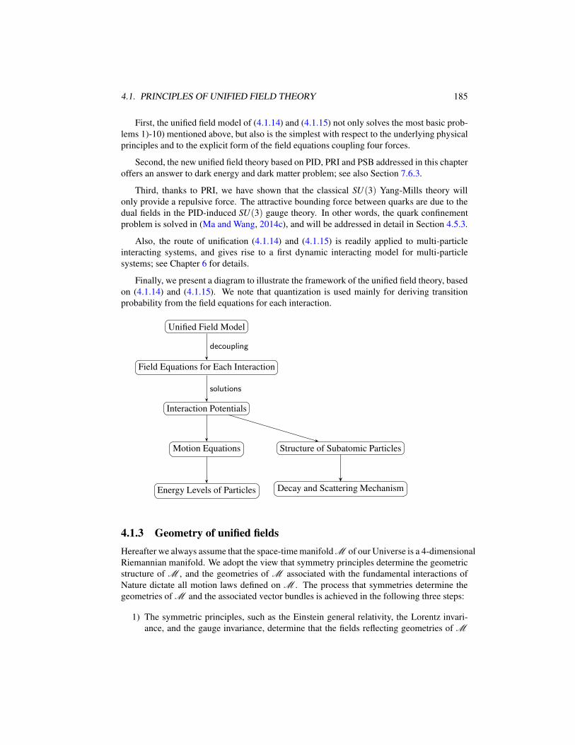
4.1. PRINCIPLES OF UNIFIED FIELD THEORY 185
First, the unified field model of (4.1.14) and (4.1.15) not only solves the most basic prob-
lems 1)-10) mentioned above, but also is the simplest with respect to the underlying physical
principles and to the explicit form of the field equations coupling four forces.
Second, the new unified field theory based on PID, PRI and PSB addressed in this chapter
offers an answer to dark energy and dark matter problem; see also Section 7.6.3.
Third, thanks to PRI, we have shown that the classical SU(3) Yang-Mills theory will
only provide a repulsive force. The attractive bounding force between quarks are due to the
dual fields in the PID-induced SU(3) gauge theory. In other words, the quark confinement
problem is solved in (Ma and Wang, 2014c), and will be addressed in detail in Section 4.5.3.
Also, the route of unification (4.1.14) and (4.1.15) is readily applied to multi-particle
interacting systems, and gives rise to a first dynamic interacting model for multi-particle
systems; see Chapter 6 for details.
Finally, we present a diagram to illustrate the framework of the unified field theory, based
on (4.1.14) and (4.1.15). We note that quantization is used mainly for deriving transition
probability from the field equations for each interaction.
Unified Field Model
Field Equations for Each Interaction
Interaction Potentials
Motion Equations Structure of Subatomic Particles
Energy Levels of Particles Decay and Scattering Mechanism
decoupling
solutions
4.1.3 Geometry of unified fields
Hereafter we always assume that the space-time manifold M of our Universe is a 4-dimensional
Riemannian manifold. We adopt the view that symmetry principles determine the geometric
structure of M , and the geometries of M associated with the fundamental interactions of
Nature dictate all motion laws defined on M . The process that symmetries determine the
geometries of M and the associated vector bundles is achieved in the following three steps:
1) The symmetric principles, such as the Einstein general relativity, the Lorentz invari-
ance, and the gauge invariance, determine that the fields reflecting geometries of M
186 CHAPTER 4. UNIFIED FIELD THEORY
are the Riemannian metric gµν and the gauge fields Gaµ. In addition, the symmet-
ric principles also determine the Lagrangian actions of gµν and Gaµ ;
2) PID determines the field equations governing gµν and Gaµ ; and
3) The solutions gµν and Gaµ of the field equations determine the geometries of M and
the vector bundles.
The geometry of the unified fields refers to the geometries of M , determined by the
following known physical symmetry principles:
(4.1.16)
principle of general relativity,
principle of Lorentz invariance,
U(1)× SU(2)× SU(3) gauge invariance,
principle of representation invariance (PRI).
We shall introduce the two principles PID and PRI in Section 4.1.5.
The fields determined by the symmetries in (4.1.16) are given by
• general relativity: gµν : M → T 02 M , the Riemannian metric,
• Lorentz invariance: ψ : M → M ⊗p (C4)N , the Dirac spinor fields,
• U(1) gauge invariance: Aµ : M → T ∗M , the U(1) gauge field,
• SU(2) gauge invariance: W aµ : M → (T ∗M )3, the SU(2) gauge fields,
• SU(3) gauge invariance: Skµ : M → (T ∗M )8, the SU(3) gauge fields.
The Lagrange action for the geometry of the unified fields is given by
(4.1.17) L =
∫
M
[LEH +LEM +LW +LS +LD]√−gdx
where LEH , LEM, LW and LS are the Lagrangian actions for the four interactions defined
by (4.1.5)–(4.1.8), and the action for the Dirac spinor fields is given by
(4.1.18) LD = Ψ(iγµ Dµ −m)Ψ.
Here
Ψ = (ψe,ψw,ψs),
m = (me,mw,ms),
and
(4.1.19)
ψe : M → M ⊗p C4 1-component Dirac spinor,
ψw : M → M ⊗p (C4)2 2-component Dirac spinors,
ψs : M → M ⊗p (C4)3 3-component Dirac spinors.
4.1. PRINCIPLES OF UNIFIED FIELD THEORY 187
The derivative operators Dµ are given by
(4.1.20)
Dµψe = (∂µ + ieAµ)ψe,
Dµψw = (∂µ + igwW aµ σa)ψ
w,
Dµψs = (∂µ + igsSkµτk)ψ
s.
The geometry of unified fields consists of 1) the field functions and 2) the Lagrangian
action (4.1.17), which are invariant under the following seven transformations:
1) the general linear transformation Qp = (aµν ) : TpM → TpM with Q−1
p = (bµν )
T , for
any p ∈ M :
(4.1.21)
(gµν) = Qp(gµν)QTp ,
Aµ = aνµAν ,
W aµ = aν
µW aν for 1 ≤ a ≤ 3,
Skµ = aν
µSkν for 1 ≤ k ≤ 8,
γµ = bµν γν , ∂µ = aν
µ∂ν ,
with no change on other fields, where γµ are the Dirac matrices;
2) the Lorentz transformation on TpM :
(4.1.22)
L = (lνµ) : TpM → TpM , L is independent of p ∈ M,
(gµν) = L(gµν )LT , Aµ = lν
µ Aν ,
W aµ = lν
µW aν for 1 ≤ a ≤ 3,
Skµ = lν
µ Skν for 1 ≤ k ≤ 8,
Ψ = RLΨ, RL is the spinor transformation matrix,
∂µ = lνµ∂ν ,
with no change on other fields;
3) the U(1) gauge transformation on M ⊗p C4:
(4.1.23)
Ω = eiθ : C4 → C
4 ∈U(1),(
ψe, Aµ
)=
(eiθ ψe,Aµ − 1
e∂µθ
),
4) SU(2) gauge transformation on M ⊗p (C4)2:
(4.1.24)
Ω = eiθ aσa : (C4)2 → (C4)2 ∈ SU(2),(
ψw,W aµ σa, mw
)=
(Ωψw,W a
µ ΩσaΩ−1 +i
gw
∂µΩΩ−1,ΩmwΩ−1
).

188 CHAPTER 4. UNIFIED FIELD THEORY
5) SU(3) gauge transformation on M ⊗p (C4)3:
(4.1.25)
Ω = eiθ kτk : (C4)3 → (C4)3 ∈ SU(3),(
ψs, Skµτk, ms
)=
(Ωψs,Sk
µΩτkΩ−1 +i
gs
∂µΩΩ−1,ΩmsΩ−1
).
6) SU(2) representation transformation on TeSU(2):
(4.1.26)
X = (xba) : TeSU(2)→ TeSU(2), (ya
b)T = X−1,
σs = xbaσb, (Gw
ab) = X(Gwab)X
T ,
W aµ = ya
bW bµ .
7) SU(3) representation transformation on TeSU(3):
(4.1.27)
X = (xlk) : TeSU(3)→ TeSU(3), (yk
l )T = X−1,
τk = xlkτl , (Gs
kl) = X(Gskl)X
T ,
Skµ = yk
l Slµ .
Remark 4.3. Here we adopt the linear transformations of the bundle spaces instead of the
coordinate transformations in the base manifold M . In this case, the two transformations
(4.1.21) and (4.1.22) are compatible. Otherwise, we have to introduce the Vierbein tensors to
overcome the incompatibility between the Lorentz transformation and the general coordinate
transformation.
4.1.4 Gauge symmetry-breaking
In physics, symmetries are displayed in two levels in the laws of Nature:
the invariance of Lagrangian actions L,(4.1.28)
the covariance of variation equations of L.(4.1.29)
The following three symmetries:
(4.1.30)
the Einstein principle of general relativity (PGR),
the Lorentz invariance,
the principle of representation invariance (PRI),
represent the universality of physical laws— the validity of laws of Nature is independent of
the coordinate systems expressing them. Consequently, the symmetries in (4.1.30) cannot be
broken at both levels of (4.1.28) and (4.1.29).
The physical implication of the gauge symmetry, however, is different at the two levels:
(1) the gauge invariance of the Lagrangian action, (4.1.28), says that the energy contribu-
tions of particles in a physical system are indistinguishable; and
4.1. PRINCIPLES OF UNIFIED FIELD THEORY 189
(2) the gauge invariance of the variational equations, (4.1.29), means that the particles
involved in the interaction are indistinguishable.
It is clear that the first aspect (1) above is universally true, while the second aspect (2) is
not universally true. In other words, the Lagrange actions obey the gauge invariance, but the
corresponding variational equations break the gauge symmetry. This suggests us to postulate
the following principle of gauge symmetry breaking for interactions described by the gauge
theory.
Principle 4.4 (Gauge Symmetry Breaking).
1) The gauge symmetry holds true only for the Lagrangian actions for the electromag-
netic, week and strong interactions; and
2) the field equations of these interactions spontaneously break the gauge symmetry.
The principle of gauge symmetry breaking can be regarded as part of the spontaneous
symmetry breaking, which is a phenomenon appearing in various physical fields. In 2008,
the Nobel Prize in Physics was awarded to Y. Nambu for the discovery of the mechanism of
spontaneous symmetry breaking in subatomic physics. In 2013, F. Englert and P. Higgs were
awarded the Nobel Prize for the theoretical discovery of a mechanism that contributes to our
understanding of the origin of mass of subatomic particles.
This phenomenon was discovered in superconductivity by Ginzburg-Landau in 1951, and
the mechanism of spontaneous symmetry breaking in particle physics was first proposed by
Y. Nambu in 1960; see (Nambu, 1960; Nambu and Jona-Lasinio, 1961a,b). The Higgs mech-
anism, introduced in (Higgs, 1964; Englert and Brout, 1964; Guralnik, Hagen and Kibble,
1964), is an artificial method based on the Nambo-Jona-Lasinio spontaneous symmetry break-
ing, leading to the mass generation for the vector bosons of the weak interaction.
PID discovered by the authors, to be stated in detail in the next section, provides a new
mechanism for gauge symmetry breaking and mass generation. The difference between the
PID and the Higgs mechanisms is that the first one is a natural sequence of the first prin-
ciple, and the second is to add artificially a Higgs field in the Lagrangian action. Also, the
PID mechanism obeys PRI, and the Higgs mechanism violates PRI. symmetry-breaking!PID-
induced
4.1.5 PID and PRI
The main objective in this subsection is to postulate two fundamental principles of physics,
the principle of interaction dynamics (PID) and the principle of representation invariance
(PRI), which are based on rigorous mathematical foundations established in Sections 3.3-3.5.
Let M ,gµν be the 4-dimensional space-time Riemannian manifold with gµν the
Minkowski type Riemannian metric. For an (r,s)-tensor u we define the A-gradient and A-
divergence operators ∇A and divA as
∇Au = ∇u+ u⊗A,
divAu = div u−A ·u,
where A is a vector field and here stands for a gauge field, ∇ and div are the usual gradient
and divergent covariant differential operators. Let F = F(u) be a functional of a tensor field
190 CHAPTER 4. UNIFIED FIELD THEORY
u. A tensor u0 is called an extremum point of F with the divA-free constraint, if u0 satisfies
the equation
(4.1.31)d
dλ
∣∣∣λ=0
F(u0 +λ X) =
∫
M
δF(u0) ·X√−gdx = 0 ∀X with divAX = 0.
Principle 4.5 (Principle of Interaction Dynamics).
1) For all physical interactions there are Lagrangian actions
(4.1.32) L(g,A,ψ) =
∫
M
L (gµν ,A,ψ)√−gdx,
where g = gµν is the Riemannian metric representing the gravitational potential, A
is a set of vector fields representing the gauge potentials, and ψ are the wave functions
of particles;
2) The action (4.1.32) satisfy the invariance of general relativity, Lorentz invariance,
gauge invariance and the gauge representation invariance;
3) The states (g,A,ψ) are the extremum points of (4.1.32) with the divA-free constraint
(4.1.31).
Based on PID and Theorems 3.26 and 3.27, the field equations with respect to the action
(4.1.32) are given in the form
δ
δgµνL(g,A,ψ) = (∇µ +αbAb
µ)Φν ,(4.1.33)
δ
δAaµ
L(g,A,ψ) = (∇µ +β ab Ab
µ)ϕa,(4.1.34)
δ
δψL(g,A,ψ) = 0(4.1.35)
where Aaµ = (Aa
0,Aa1,A
a2,A
a3) are the gauge vector fields for the electromagnetic, the weak and
strong interactions, Φν = (Φ0,Φ1,Φ2,Φ3) in (4.1.33) is a vector field induced by gravita-
tional interaction, ϕa is the scalar fields generated from the gauge fields Aaµ , and αb,β
ab are
coupling parameters.
Consider the action (4.1.32) as the natural combination of the actions for all four interac-
tions, as given in (4.1.17)-(4.1.20):
L = LEH +LEM +LW +LS +LD.
Then (4.1.33)-(4.1.35) provide the unified field equations coupling all interactions. Moreover,
we see from (4.1.33)-(4.1.35) that there are too many coupling parameters which need to
be determined. Fortunately, this problem can be satisfactorily resolved, leading also to the
discovery of PRI (Ma and Wang, 2014h). Meanwhile, we remark that it is the gauge fields
Aaµ appearing on the right-hand sides of (4.1.33) and (4.1.34) that break the gauge symmetry,
leading to the mass generation of the vector bosons for the weak interaction sector.
4.1. PRINCIPLES OF UNIFIED FIELD THEORY 191
We are now in position to introduce the principle of representation invariance (PRI). We
end this section by recalling the principle of representation invariance (PRI) first postulated
in (Ma and Wang, 2014h). We proceed with the SU(N) representation. In a neighborhood
U ⊂ SU(N) of the unit matrix, a matrix Ω ∈U can be written as
Ω = eiθ aτa ,
where
(4.1.36) τa = τ1, · · · ,τK ⊂ TeSU(N), K = N2 − 1,
is a basis of generators of the tangent space TeSU(N); see Section 3.5 for the mathematical
theory. An SU(N) representation transformation is a linear transformation of the basis in
(4.1.36) as
(4.1.37) τa = xbaτb,
where X = (xba) is a nondegenerate complex matrix.
Mathematical logic dictates that a physically sound gauge theory should be invariant un-
der the SU(N) representation transformation (4.1.37). Consequently, the following princi-
ple of representation invariance (PRI) must be universally valid and was first postulated in
(Ma and Wang, 2014h).
Principle 4.6 (Principle of Representation Invariance). All SU(N) gauge theories are invari-
ant under the transformation (4.1.37). Namely, the actions of the gauge fields are invariant
and the corresponding gauge field equations as given by (4.1.33)-(4.1.35) are covariant un-
der the transformation (4.1.37).
Both PID and PRI are very important. As far as we know, it appears that the only unified
field model, which obeys not only PRI but also the principle of gauge symmetry breaking,
Principle 4.4, is the unified field model based on PID introduced in this chapter. From this
model, we can derive not only the same physical conclusions as those from the standard
model, but also many new results and predictions, leading to the solution of a number of
longstanding open questions in physics, including the 10 problems mentioned in Section
4.1.2.
A few further remarks on PID and PRI are now in order.
First, there are strong theoretical, experimental and observational evidence for PID; see
the next section for details.
Second, PID is based on variations with divA-free constraint defined by (4.1.31). Phys-
ically, the divA-free condition: divAX = 0 stands for the energy-momentum conservation
constraints.
Third, PRI means that the gauge theory is universally valid, and therefore should be in-
dependent of the choice of the generators τa of SU(N). In other words, PRI is basic a logic
requirement.
Fourth, the electroweak interactions is a U(1)× SU(2) gauge theory coupled with the
Higgs mechanism. An unavoidable feature for the Higgs mechanism is that the gauge fields
192 CHAPTER 4. UNIFIED FIELD THEORY
with different symmetry groups are combined linearly into terms in the corresponding gauge
field equations. For example, in the Weinberg-Salam electroweak gauge equations with
U(1)× SU(2) symmetry breaking, there are such linearly combinations as
(4.1.38)
Zµ = cosθWW 3µ + sinθW Bµ ,
Aµ =−sinθWW 3µ + cosθW Bµ ,
W±µ =
1√2(W 1
µ ± iW2µ ),
where W aµ (1 ≤ a ≤ 3) are the SU(2) gauge fields, and Bµ is the U(1) gauge field. It is
clear that these terms in (4.1.38) are not covariant under the general SU(2) representation
transformations. Hence, the Higgs mechanism violates the PRI. Since the standard model is
based on the Higgs mechanism, it violates PRI as well.
4.2 Physical Supports to PID
The original motivation for PID was to explain the dark matter and dark energy phenomena.
We have demonstrated that the presence of dark matter and dark energy leads directly to PID
for gravity.
There are strong theoretical, experimental and observational evidence for PID. The need
of spontaneous symmetry-breaking for generating mass of the vector bosons for the weak
interaction is a physical evidence for PID for the weak interaction. The quark confinement
requires the introduction of the dual gluon fields demonstrates the necessity of PID; see Sec-
tion 4.5. In this section, we address the physical evidence from the following viewpoints:
1) the discovery of dark matter and dark energy,
2) the non-existence of solutions for the classical Einstein gravitational field equations in
general situations,
3) the principle of spontaneous gauge-symmetry breaking,
4) the Ginzburg-Landau superconductivity theory, and
5) the gauge-fixing problem.
4.2.1 Dark matter and dark energy
The presence of dark matter and dark energy provides a strong support for PID. We recall the
Einstein gravitational equations, which are expressed as
(4.2.1) Rµν −1
2gµνR =−4πG
c4Tµν ,
where Tµν is the usual energy-momentum tensor of visible matter. By the Bianchi identity,
the left-hand side of (4.2.1) is divergence-free, i.e.
(4.2.2) ∇µ(Rµν −1
2gµνR) = 0.
4.2. PHYSICAL SUPPORTS TO PID 193
It implies that the usual energy-momentum tensor satisfies
(4.2.3) ∇µTµν = 0.
However, due to the presence of dark matter and dark energy, the energy-momentum
tensor of visible matter Tµν may no longer be conserved, i.e. (4.2.3) is not true. Hence we
have
∇µTµν 6= 0,
which is a contradiction to (4.2.1) and (4.2.2).
On the other hand, by the Orthogonal Decomposition Theorem 3.17, Tµν can be orthog-
onally decomposed into
(4.2.4) Tµν = Tµν −c4
8πG∇µΦν ,
and Tµν is divergence-free:
(4.2.5) ∇µ Tµν = 0.
Hence, by (4.2.2) and (4.2.5) the gravitational field equations (4.2.1) should be in the form
(4.2.6) Rµν −1
2gµνR =−8πG
c4Tµν .
By (4.2.4) we have
Tµν = Tµν +c4
8πG∇µΦν ,
which stands for all energy and momentum including the visible and the invisible matter and
energy, and which, by (4.2.5), is conserved. Thus, the equations (4.2.6) are rewritten as
(4.2.7) Rµν −1
2gµνR =−8πG
c4Tµν −∇µΦν ,
The equations (4.2.7) are just the variational equations of LEH with the div-free constraint as
(4.1.33). Namely, (4.2.7) are the gravitational field equations obeying PID.
We remark that the term ∇µΦν in (4.2.7) has no variational structure, and cannot be
derived by modifying the Einstein-Hilbert functional. Hence, (4.2.7) are just the variational
equations due to PID.
4.2.2 Non well-posedness of Einstein field equations
The second strong theoretical evidence to PID is that the classical Einstein gravitational field
equations are an over-determined system.
The Einstein field equations (4.2.1) possess 10 unknown functions gµν and 10 indepen-
dent equations due to symmetry for the indices µ and ν . However, since the general coordi-
nate system can be arbitrarily chosen, under proper coordinate transformation
xµ = aνµxν , 0 ≤ ν ≤ 3,
194 CHAPTER 4. UNIFIED FIELD THEORY
the 10 unknown functions become(−1 0
0 gi j
), gi j = g ji for 1 ≤ i, j ≤ 3.
This observation implies that the number of independent unknown functions for the Einstein
field equations (4.2.1) is six. Namely,
(4.2.8)NEQ = 10,
NUF = 6,
where NEQ is the number of independent equations in (4.2.1), and NUF is the number of
independent unknown functions.
Consequently, the Einstein field equations (4.2.1) have no solutions in the general case.
Some readers may think that the Bianchi identity
(4.2.9) ∇µ
(Rµν −
1
2gµνR+
8πG
c4Tµν
)= 0,
reduce the number NEQ to six: NEQ = 6. But we note that (4.2.9) generates also four new
equations
∇µ Tµν = 0 for 0 ≤ ν ≤ 3,
because there are unknown functions gµν in the covariant derivative operators ∇µ ; see (3.1.66)
or (2.3.26). Hence, the Einstein field equations (4.2.1) should be in the form
(4.2.10)Rµν −
1
2gµνR =−8πG
c4Tµν ,
∇µ Tµν = 0.
Thus, the fact (4.2.8) still holds for (4.2.10).
Now we note the gravitational field equations (4.2.7) derived from PID, where there are
four additional new unknown functions Φν (0 ≤ ν ≤ 3). In this case, the numbers of inde-
pendent unknown functions and equations are the same.
In the following, we give an example to show the non well-posedness of the classical
Einstein field equations.
It is known that the metric of central gravitational field takes the form
(4.2.11) ds2 = c2g00dt2 + g11dr2 + r2(dθ 2 + sin2 θdϕ2),
where (ct,r,θ ,ϕ) is the spherical coordinate system. The metric gµν in (4.2.11) can be ex-
pressed in the form
(4.2.12)
g00 =−eu (u = u(r)),
g11 = ev (v = v(r)),
g22 = r2,
g33 = r2 sin2 θ ,
gµν = 0 for µ 6= ν.
4.2. PHYSICAL SUPPORTS TO PID 195
Consider the influence of cosmic microwave background (CMB) radiation, the energy-
momentum tensor can be approximatively written as
(4.2.13) Tµν =
(−g00ρ 0
0 0
),
where ρ is the energy density, a constant.
For the metric (4.2.12), the nonzero components of the Ricci tensor are
(4.2.14)
R00 =−eµ−ν
[u′′
2+
u′
r+
u′
4(u′− v′)
],
R11 =u′′
2− v′
r+
u′
4(u′− v′),
R22 = e−v[1− ev+
r
2(u′− v′)
],
R33 = sin2 θR22.
On the other hand, equations (4.2.10) can be equivalently written as
(4.2.15)Rµν =−8πG
c4(Tµν −
1
2gµνT ),
∇µTµν = 0,
and by (4.2.13),
T = gµνTµν = g00T00 =−ρ .
Thus, the Einstein field equations for the spherically symmetric gravitation fields (4.2.15) are
in the form
(4.2.16)
R00 =4πG
c4g00ρ ,
R11 =−4πG
c4g11ρ ,
R22 =−4πG
c4g22ρ ,
∇µ Tµν = 0.
Now, we deduce that the equations (4.2.16) have no solutions. By DµTµν = 0, we have
Γ010T00 =
1
2u′ρ = 0,
which implies that u′ = 0. Hence, by (4.2.14) we have
R00 = 0,
which is a contradiction to the first equation of (4.2.16). Therefore the equations (4.2.16)
have no solutions.
However, if we consider this example by using the field equations derived from PID, then
the problem must have a solutions; see the theory of dark matter and dark energy in Chapter
7.
196 CHAPTER 4. UNIFIED FIELD THEORY
4.2.3 Higgs mechanism and mass generation
Principle 4.4 of gauge symmetry breaking is also a main motivation to postulate PID in our
program for a unified field theory. In fact, the Higgs mechanism is one way to achieve
the spontaneous gauge-symmetry breaking. In the Glashow-Weinberg-Salam (GWS) elec-
troweak theory, the three intermediate vector bosons W± and Z for the weak interaction re-
tain their masses by the Higgs mechanism. We now show that the masses of the intermediate
vector bosons can be also obtained by PID. Furthermore, we shall show in Section 4.6 that
all conclusions of the GWS electroweak theory confirmed by experiments can be derived by
the unified field theory based on PID.
For convenience, we first introduce some related basic knowledge of quantum physics.
In quantum field theory, a field ψ is called a fermion with mass m, if it satisfies the Dirac
equation
(4.2.17) (iγµDµ −m)ψ = 0,
and the action of (4.2.17) is
(4.2.18) LF =
∫LF dx, LF = ψ(iγµ Dµ −m)ψ ,
where ψ = ψ†γ0.
A field Φ is called a boson with mass m, if Φ satisfies a Klein-Gordon type of wave
equation:
(4.2.19) Φ+(mc
h
)2
Φ = g(Φ),
where g(Φ) is the terms of Φ other than kΦ (k a constant), and is the wave operator given
by
=−∂ µ∂µ =1
c2
∂ 2
∂ t2−∆.
The bosonic field Φ is massless if it satisfies
(4.2.20) Φ = g(Φ).
The physical significances of the fermionic and bosonic fields ψ and Φ are as follows:
1) Macro-scale: ψ and Φ represent field energy density. In particular, if Φ is a gauge field
then it stands for the interaction potential corresponding to the gauge theory.
2) Micro-scale (Quantization): ψ represents a spin- 12
fermionic particle, and Φ represents
a bosonic particle with an integer spin k if Φ is a k-th order tensor field.
In particular, in the classical Yang-Mills theory, the SU(N) gauge fields Aaµ =(Aa
0,Aa1,A
a2,A
a3)
(1 ≤ a ≤ N2 − 1) satisfy the following field equations:
(4.2.21) ∂ µFaµν = o(Aµ), Fa
µν = ∂µ Aaν − ∂νAa
µ + gλ abcA
bµAc
ν ,
4.2. PHYSICAL SUPPORTS TO PID 197
which are the variational equations of the Yang-Mills action
(4.2.22) LY M =
∫−1
4Fa
µνF µνa +LFdx,
where LF is as in (4.2.18) with Dµ = ∂µ + igAaµτa, and
∂ µ Faµν =−Aa
ν − ∂ν(∂µAa
µ)+ o(A).
Thus, the gauge field equations (4.2.21) are reduced to the bosonic field equations (4.2.20).
In other words, the gauge fields Aaµ (1 ≤ a ≤ N2 − 1) satisfying (4.2.21) represent N2 − 1
massless bosons with spin-1 because each Aaµ is a vector field.
We are now in position to introduce the Higgs mechanism. Physical experiments show
that the weak interacting fields should be SU(2) gauge fields with masses, representing 3
massive bosonic particles. However, as mentioned in (4.2.21), the gauge fields satisfying
the SU(2) Yang-Mills theory are 3(= N2 − 1) massless bosons. To overcome this difficulty,
(Higgs, 1964; Englert and Brout, 1964; Guralnik, Hagen and Kibble, 1964) suggested to add
a scalar field φ into the Yang-Mills action (4.2.22) to create masses. In fact, we cannot add a
massive term mAaµAµa into the Yang-Mills action (4.2.22); otherwise this action will violate
the gauge symmetry. But the Higgs mechanism can ensure the gauge invariance for the Yang-
Mills action, and spontaneously break the gauge symmetry in field equations at a ground state
of the Higgs field φ .
For clearly revealing the essence of the Higgs mechanism, we only take one gauge field
(there are four gauge fields in the GWS theory). In this case, the Yang-Mills action density is
in the form
(4.2.23) LYM =−1
4gµα gνβ (∂µAν − ∂νAµ)(∂α Aβ − ∂β Aα)+ψ(iγµDµ −m)ψ ,
where gµν is the Minkowski metric, and
(4.2.24) Dµ ψ = (∂µ + igAµ)ψ .
It is clear that the action (4.2.23) is invariant under the following U(1) gauge transformation
(4.2.25) ψ → eiθ ψ , Aµ → Aµ −1
g∂µθ .
The variation equations of (4.2.23) are
(4.2.26)
Aµ + ∂µ(∂ν Aν)+ gJµ = 0,
(iγµDµ −m)ψ = 0,
Jµ = ψγµψ ,
which are invariant under the gauge transformation (4.2.25). It is clear that the bosonic parti-
cle Aµ in (4.2.26) is massless.
To generate mass for Aµ , we add a Higgs sector LH to the Yang-Mills action (4.2.23):
(4.2.27)
LH =−1
2gµν(Dµφ)†(Dµφ)+
1
4(φ†φ −ρ2)2,
Dµφ = (∂µ + igAµ)φ ,
(Dµφ)† = (∂µ − igAµ)φ†,
198 CHAPTER 4. UNIFIED FIELD THEORY
where ρ 6= 0 is a constant. Obviously, the following action
(4.2.28) L =
∫(LYM +LH)dx,
and its variational equations
δL
δAµ= ∂ ν (∂νAµ − ∂µAν)− gJµ −
ig
2(φ(Dµ φ)† −φ†Dµφ) = 0,
δL
δψ= (iγµ Dµ −m)ψ = 0,(4.2.29)
δL
δφ= DµDµφ +(φ2 −ρ2)φ = 0,
are invariant under the gauge transformation
(4.2.30) (ψ ,φ)→ (eiθ ψ ,eiθ φ), Aµ → Aµ −1
g∂µθ .
Equations (4.2.29) are still massless. However, we note that (0,0,ρ) is a solution of
(4.2.29), which represents a ground state in physics, i.e. a vacuum state. Consider a transla-
tion for Φ = (A,ψ ,φ) at Φ0 = (0,0,ρ) as
Φ = Φ+Φ0, Φ = (A, ψ , φ ),
then the equations (4.2.29) become
(4.2.31)
∂ ν (∂ν Aµ − ∂µ Aν)− g2ρ2Aµ − gJµ + gJµ(φ) = 0,
(iγµ Dµ −m)ψ = 0,
DµDµ(φ +ρ)− 2ρ2φ +(φ +ρ)φ2 = 0,
where
Jµ(φ) =i
2(φ (Dµ φ)† − φ†Dµ φ ).
We see that Aµ attains its mass m = gρ in (4.2.31), but equations (4.2.31) break the
invariance for the gauge transformation (4.2.30). The process that masses are created by the
spontaneous gauge-symmetry breaking is called the Higgs mechanism. Meanwhile, the field
φ in (4.2.31), called the Higgs boson, is also obtain its mass m =√
2ρ .
In the following, we show that PID provides a new mechanism for generating masses,
drastly different from the Higgs mechanism.
In view of (4.1.34) and (4.1.35), based on PID, the variational equations of the Yang-Mills
action (4.2.23) with the divA-free constraint are in the form
(4.2.32)∂ ν(∂ν Aµ − ∂µAν)− gJµ =
[∂µ − 1
4
(mc
h
)2
xµ +λ Aµ
]φ ,
(iγµDµ −m f )ψ = 0,
4.2. PHYSICAL SUPPORTS TO PID 199
where φ is a scalar field. The term − 14
(mch
)2xµ is the mass potential of φ , and is also regarded
as the interacting length of φ . If φ has a nonzero ground state φ0 = ρ , then for the translation
φ = φ +ρ , Aµ = Aµ , ψ = ψ ,
the first equation of (4.2.32) becomes
(4.2.33) ∂ ν (∂ν Aµ − ∂µ Aν)−(m0c
h
)2
Aµ − gJµ =
[∂µ − 1
4
(mc
h
)2
xµ +λ Aµ
]φ ,
where(
m0ch
)2= λ ρ . Thus the mass m0 =
hc
√λ ρ is generated in (4.2.33) as the Yang-Mills
action takes the divA-free constraint variation. Moreover, when we take divergence on both
sides of (4.2.33), and by
∂ µ ∂ ν(∂ν Aµ − ∂µ Aν) = 0, ∂ µ Jµ = 0,
we derive the field equation of φ as follows
(4.2.34) ∂ µ∂µ φ −(mc
h
)2
φ =−λ ∂ µ(Aµ φ )+1
4
(mc
h
)2
xµ∂ µ φ .
This equation (4.2.34) is the field equation with mass m for the Higgs bosonic particle φ .
Remark 4.7. In (4.2.28) we see that the essence of the Higgs mechanism is to add artificially
a Higgs sector LH into the Yang-Mills action. However, for the PID model, the masses of Aµ
and the Higgs field φ are generated naturally for the first principle, PID, taking the variation
with energy-momentum conservation constraint.
4.2.4 Ginzburg-Landau superconductivity
Superconductivity studies the behavior of the Bose-Einstein condensation and electromag-
netic interactions. The Ginzburg-Landau theory provides a support for PID.
The Ginzburg-Landau free energy for superconductivity is
(4.2.35) G =
∫
Ω
[1
2ms
∣∣∣(
ih∇+es
cA
)ψ∣∣∣2
+ a|ψ |2 + b
2|ψ |4 + 1
8π| curl A|2
]dx
where A is the electromagnetic potential, ψ is the wave function of superconducting electrons,
Ω is the superconductor, es and ms are charge and mass of a Cooper pair.
The superconducting current equations determined by the Ginzburg-Landau free energy
(4.2.35) are:
(4.2.36)δG
δA= 0,
which implies that
(4.2.37)c
4πcurl2A =− e2
s
msc|ψ |2A− i
hes
ms
(ψ∗∇ψ −ψ∇ψ∗).
200 CHAPTER 4. UNIFIED FIELD THEORY
Let
J =c
4πcurl2A, Js =
e2s
msc|ψ |2A− i
hes
ms
(ψ∗∇ψ −ψ∇ψ∗).
Physically, J is the total current in Ω, and Js is the superconducting current. Since Ω is a
medium conductor, J contains two types of currents as
J = Js +σE,
where σ is dielectric constant, σE is the current generated by the electric field E ,
E =−1
c
∂A
∂ t−∇Φ =−∇Φ,
and Φ is the electric potential. Since At = 0, the superconducting current equations should be
taken as
(4.2.38)1
4πcurl2A =−σ
c∇Φ− e2
s
msc2|ψ |2A− ihes
msc(ψ∗∇ψ −ψ∇ψ∗).
Since (4.2.37) is the expression of (4.2.36), then the equation (4.2.38) can be written in
the abstract form
(4.2.39)δG
δA=−σ
c∇Φ.
In addition, for conductivity, the gauge fixing is given by
div A = 0, A ·n|∂Ω = 0,
which imply that ∫
Ω∇Φ ·Adx = 0.
Hence, the term −σc
∇Φ in (4.2.39) can not be added into the Ginzburg-Landau free energy
(4.2.35).
However, the equation (4.2.39) are just the variational equation with divergence-free con-
straint as follows
〈δG
δA,X〉= d
dλG(A+λ X)|λ=0 = 0 ∀ div X = 0.
Thus, we see that the Ginzburg-Landau superconductivity theory obeys PID.
4.3 Unified Field Model Based on PID and PRI
4.3.1 Unified field equations based on PID
The abstract unified field equations (4.1.33)-(4.1.34) are derived based on PID. We now
present the detailed form of this model, ensuring that these field equations satisfy both the
principle of gauge-symmetry breaking, Principle 4.4, and PRI.
4.3. UNIFIED FIELD MODEL BASED ON PID AND PRI 201
In Section 4.1.3, we showed that the action functional obeys all the symmetric principles,
including principle of general relativity, the Lorentz invariance, the U(1)× SU(2)× SU(3)gauge invariance and PRI, is the natural combination of the Einstein-Hilbert functional, the
U(1),SU(2),SU(3) Yang-Mills actions for the electromagnetic, weak and strong interac-
tions:
(4.3.1) L =
∫
M
[LEH +LEM +LW +LS]√−gdx.
Here
(4.3.2)
LEH = R+8πG
c4S,
LEM =−1
4AµνAµν +ψe(iγµDµ −m)ψe,
LW =−1
4G
wabW a
µνW bµν +ψw(iγµ Dµ −ml)ψw,
LS =−1
4G
sklS
kµνSµνl +ψs(iγµDµ −mq)ψ
s,
where R is the scalar curvature of the space-time Riemannian manifold (M ,gµν) with Minkowski
type metric, S is the energy-momentum density, G wab and G s
kl are the SU(2) and SU(3) metrics
as defined by (3.5.28), ψe, ψw and ψs are the Dirac spinors for fermions participating in the
electromagnetic, weak, strong interactions, and
(4.3.3)
Aµν = ∂µAν − ∂νAµ ,
W aµν = ∂µW a
ν − ∂νW aµ + gwλ a
bcWbµW c
ν ,
Skµν = ∂µ Sk
ν − ∂νSkµ + gsΛ
klrSl
µSrν .
Here Aµ is the electromagnetic potential, W aµ (1 ≤ a ≤ 3) are the SU(2) gauge fields for the
weak interaction, Skµ (1 ≤ k ≤ 8) are the SU(3) gauge fields for the strong interaction, gw and
gs are the weak and strong charges, and
(4.3.4)
Dµψe = (∂µ + ieAµ)ψe,
Dµψw = (∂µ + igwW aµ σa)ψ
w,
Dµψs = (∂µ + igsSkµτk)ψ
s,
where σa (1 ≤ a ≤ 3) and τk (1 ≤ k ≤ 8) are the generators of SU(2) and SU(3).
Remark 4.8. For a vector field Xµ and an antisymmetric tensor field Fµν , we have
∇µXν −∇νXµ = ∂µXν − ∂νXµ ,
∇µFµν = ∂ µ Fµν ,
where ∇µ is the Levi-Civita covariant derivative. Hence, the tensor fields in (4.3.3) and the
action (4.3.1) obey both the Einstein general relativity and the Lorentz invariance simultane-
ously under the transformations (4.1.21)-(4.1.22).
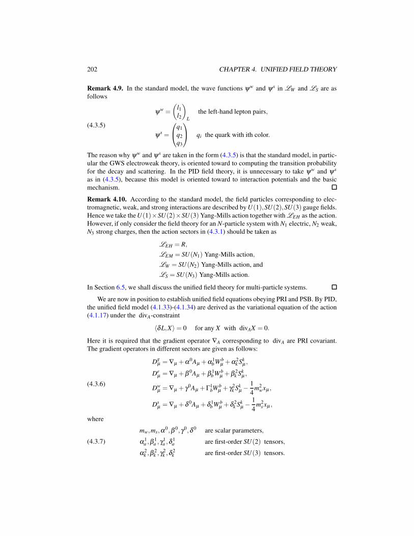
202 CHAPTER 4. UNIFIED FIELD THEORY
Remark 4.9. In the standard model, the wave functions ψw and ψs in LW and LS are as
follows
(4.3.5)
ψw =
(l1l2
)
L
the left-hand lepton pairs,
ψs =
q1
q2
q3
qi the quark with ith color.
The reason why ψw and ψs are taken in the form (4.3.5) is that the standard model, in partic-
ular the GWS electroweak theory, is oriented toward to computing the transition probability
for the decay and scattering. In the PID field theory, it is unnecessary to take ψw and ψs
as in (4.3.5), because this model is oriented toward to interaction potentials and the basic
mechanism.
Remark 4.10. According to the standard model, the field particles corresponding to elec-
tromagnetic, weak, and strong interactions are described by U(1),SU(2),SU(3) gauge fields.
Hence we take the U(1)×SU(2)×SU(3)Yang-Mills action together with LEH as the action.
However, if only consider the field theory for an N-particle system with N1 electric, N2 weak,
N3 strong charges, then the action sectors in (4.3.1) should be taken as
LEH = R,
LEM = SU(N1) Yang-Mills action,
LW = SU(N2) Yang-Mills action, and
LS = SU(N3) Yang-Mills action.
In Section 6.5, we shall discuss the unified field theory for multi-particle systems.
We are now in position to establish unified field equations obeying PRI and PSB. By PID,
the unified field model (4.1.33)-(4.1.34) are derived as the variational equation of the action
(4.1.17) under the divA-constraint
〈δL,X〉= 0 for any X with divAX = 0.
Here it is required that the gradient operator ∇A corresponding to divA are PRI covariant.
The gradient operators in different sectors are given as follows:
(4.3.6)
Dgµ = ∇µ +α0Aµ +α1
bW bµ +α2
k Skµ ,
Deµ = ∇µ +β 0Aµ +β 1
b W bµ +β 2
k Skµ ,
Dwµ = ∇µ + γ0Aµ +Γ1
bW bµ + γ2
k Skµ −
1
4m2
wxµ ,
Dsµ = ∇µ + δ 0Aµ + δ 1
b W bµ + δ 2
k Skµ −
1
4m2
s xµ ,
where
(4.3.7)
mw,ms,α0,β 0,γ0,δ 0 are scalar parameters,
α1a ,β
1a ,γ
1a ,δ
1a are first-order SU(2) tensors,
α2k ,β
2k ,γ
2k ,δ
2k are first-order SU(3) tensors.
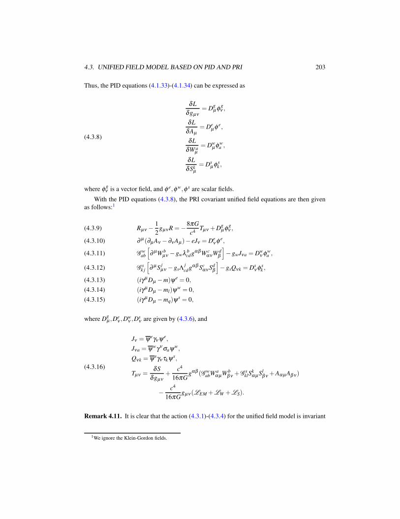
4.3. UNIFIED FIELD MODEL BASED ON PID AND PRI 203
Thus, the PID equations (4.1.33)-(4.1.34) can be expressed as
(4.3.8)
δL
δgµν= D
gµφg
ν ,
δL
δAµ= De
µφ e,
δL
δW aµ
= Dwµφw
a ,
δL
δSkµ
= Dsµφ s
k ,
where φgν is a vector field, and φ e,φw,φ s are scalar fields.
With the PID equations (4.3.8), the PRI covariant unified field equations are then given
as follows:1
Rµν −1
2gµνR =−8πG
c4Tµν +D
gµφg
ν ,(4.3.9)
∂ µ(∂µAν − ∂νAµ)− eJν = Deν φ e,(4.3.10)
Gwab
[∂ µW b
µν − gwλ bcdgαβW c
ανW dβ
]− gwJνa = Dw
ν φwa ,(4.3.11)
Gsk j
[∂ µS
jµν − gsΛ
j
cdgαβ ScανSd
β
]− gsQνk = Ds
νφ sk ,(4.3.12)
(iγµ Dµ −m)ψe = 0,(4.3.13)
(iγµ Dµ −ml)ψw = 0,(4.3.14)
(iγµ Dµ −mq)ψs = 0,(4.3.15)
where Dgµ ,D
eν ,D
wν ,D
sν are given by (4.3.6), and
(4.3.16)
Jν = ψeγνψe,
Jνa = ψwγν σaψw,
Qνk = ψsγν τkψs,
Tµν =δS
δgµν+
c4
16πGgαβ (G w
abW aαµW b
β ν +GsklS
kαµSl
β ν +AαµAβ ν)
− c4
16πGgµν(LEM +LW +LS).
Remark 4.11. It is clear that the action (4.3.1)-(4.3.4) for the unified field model is invariant
1We ignore the Klein-Gordon fields.
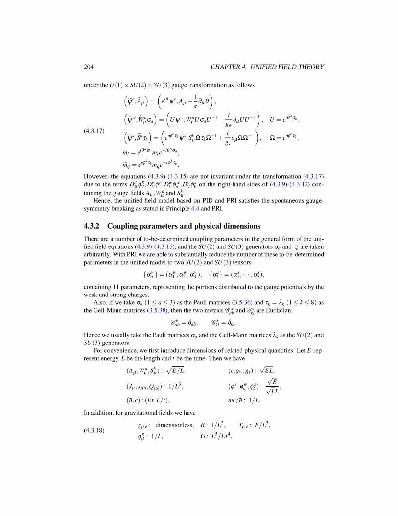
204 CHAPTER 4. UNIFIED FIELD THEORY
under the U(1)× SU(2)× SU(3) gauge transformation as follows
(4.3.17)
(ψe, Aµ
)=
(eiθ ψe,Aµ − 1
e∂µθ
),
(ψw,W a
µ σa
)=
(Uψw,W a
µUσaU−1 +i
gw
∂µUU−1
), U = eiθ aσa ,
(ψs, Skτk
)=
(eiϕkτk ψs,Sk
µΩτkΩ−1 +i
gs∂µΩΩ−1
), Ω = eiϕkτk ,
ml = eiθ aσamle−iθ aσa ,
mq = eiϕkτk mqe−iϕkτk .
However, the equations (4.3.9)-(4.3.15) are not invariant under the transformation (4.3.17)
due to the terms Dgµφg
ν ,Deν φ e,Dw
ν φwa ,D
sνφ s
k on the right-hand sides of (4.3.9)-(4.3.12) con-
taining the gauge fields Aµ ,Waµ and Sk
µ .
Hence, the unified field model based on PID and PRI satisfies the spontaneous gauge-
symmetry breaking as stated in Principle 4.4 and PRI.
4.3.2 Coupling parameters and physical dimensions
There are a number of to-be-determined coupling parameters in the general form of the uni-
fied field equations (4.3.9)-(4.3.15), and the SU(2) and SU(3) generators σa and τk are taken
arbitrarily. With PRI we are able to substantially reduce the number of these to-be-determined
parameters in the unified model to two SU(2) and SU(3) tensors
αwa = (αw
1 ,αw2 ,α
w3 ), αs
k= (αs1, · · · ,αs
8),
containing 11 parameters, representing the portions distributed to the gauge potentials by the
weak and strong charges.
Also, if we take σa (1 ≤ a ≤ 3) as the Pauli matrices (3.5.36) and τk = λk (1 ≤ k ≤ 8) as
the Gell-Mann matrices (3.5.38), then the two metrics G wab and G s
kl are Euclidian:
Gwab = δab, G
skl = δkl .
Hence we usually take the Pauli matrices σa and the Gell-Mann matrices λk as the SU(2) and
SU(3) generators.
For convenience, we first introduce dimensions of related physical quantities. Let E rep-
resent energy, L be the length and t be the time. Then we have
(Aµ ,Waµ ,S
kµ) :
√E/L, (e,gw,gs) :
√EL,
(Jµ ,Jµa,Qµk) : 1/L3, (φ e,φwa ,φ
sk ) :
√E√LL
,
(h,c) : (Et,L/t), mc/h : 1/L.
In addition, for gravitational fields we have
(4.3.18)gµν : dimensionless, R : 1/L2, Tµν : E/L3,
φgµ : 1/L, G : L5/Et4.
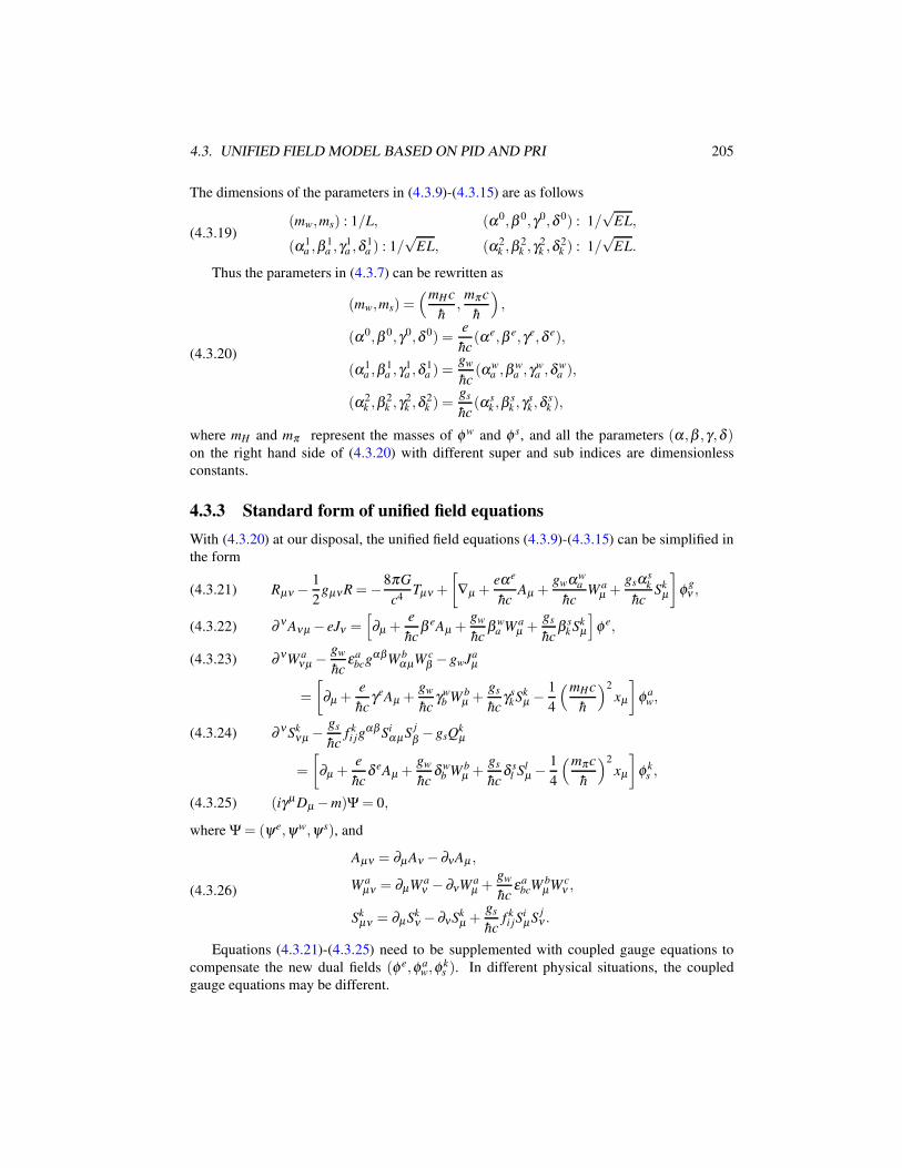
4.3. UNIFIED FIELD MODEL BASED ON PID AND PRI 205
The dimensions of the parameters in (4.3.9)-(4.3.15) are as follows
(4.3.19)(mw,ms) : 1/L, (α0,β 0,γ0,δ 0) : 1/
√EL,
(α1a ,β
1a ,γ
1a ,δ
1a ) : 1/
√EL, (α2
k ,β2k ,γ
2k ,δ
2k ) : 1/
√EL.
Thus the parameters in (4.3.7) can be rewritten as
(4.3.20)
(mw,ms) =(mHc
h,
mπ c
h
),
(α0,β 0,γ0,δ 0) =e
hc(αe,β e,γe,δ e),
(α1a ,β
1a ,γ
1a ,δ
1a ) =
gw
hc(αw
a ,βwa ,γ
wa ,δ
wa ),
(α2k ,β
2k ,γ
2k ,δ
2k ) =
gs
hc(αs
k ,βsk ,γ
sk ,δ
sk ),
where mH and mπ represent the masses of φw and φ s, and all the parameters (α,β ,γ,δ )on the right hand side of (4.3.20) with different super and sub indices are dimensionless
constants.
4.3.3 Standard form of unified field equations
With (4.3.20) at our disposal, the unified field equations (4.3.9)-(4.3.15) can be simplified in
the form
Rµν −1
2gµνR =−8πG
c4Tµν +
[∇µ +
eαe
hcAµ +
gwαwa
hcW a
µ +gsα
sk
hcSk
µ
]φg
ν ,(4.3.21)
∂ ν Aνµ − eJν =[∂µ +
e
hcβ eAµ +
gw
hcβ w
a W aµ +
gs
hcβ s
k Skµ
]φ e,(4.3.22)
∂ νW aνµ − gw
hcεa
bcgαβW bαµW c
β − gwJaµ(4.3.23)
=
[∂µ +
e
hcγeAµ +
gw
hcγw
b W bµ +
gs
hcγs
kSkµ − 1
4
(mHc
h
)2
xµ
]φa
w,
∂ ν Skνµ −
gs
hcf ki jg
αβ SiαµS
j
β− gsQ
kµ(4.3.24)
=
[∂µ +
e
hcδ eAµ +
gw
hcδ w
b W bµ +
gs
hcδ s
l Slµ −
1
4
(mπc
h
)2
xµ
]φ k
s ,
(iγµ Dµ −m)Ψ = 0,(4.3.25)
where Ψ = (ψe,ψw,ψs), and
(4.3.26)
Aµν = ∂µAν − ∂νAµ ,
W aµν = ∂µW a
ν − ∂νW aµ +
gw
hcεa
bcWbµW c
ν ,
Skµν = ∂µSk
ν − ∂νSkµ +
gs
hcf ki jS
iµS
jν .
Equations (4.3.21)-(4.3.25) need to be supplemented with coupled gauge equations to
compensate the new dual fields (φ e,φaw,φ
ks ). In different physical situations, the coupled
gauge equations may be different.
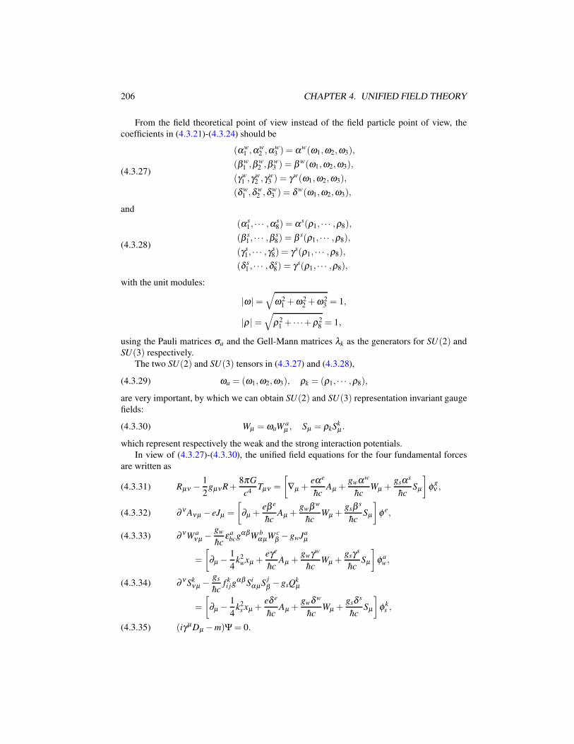
206 CHAPTER 4. UNIFIED FIELD THEORY
From the field theoretical point of view instead of the field particle point of view, the
coefficients in (4.3.21)-(4.3.24) should be
(4.3.27)
(αw1 ,α
w2 ,α
w3 ) = αw(ω1,ω2,ω3),
(β w1 ,β
w2 ,β
w3 ) = β w(ω1,ω2,ω3),
(γw1 ,γ
w2 ,γ
w3 ) = γw(ω1,ω2,ω3),
(δ w1 ,δ
w2 ,δ w
3 ) = δ w(ω1,ω2,ω3),
and
(4.3.28)
(αs1, · · · ,αs
8) = αs(ρ1, · · · ,ρ8),
(β s1 , · · · ,β s
8) = β s(ρ1, · · · ,ρ8),
(γs1, · · · ,γs
8) = γs(ρ1, · · · ,ρ8),
(δ s1 , · · · ,δ s
8) = γs(ρ1, · · · ,ρ8),
with the unit modules:
|ω |=√
ω21 +ω2
2 +ω23 = 1,
|ρ |=√
ρ21 + · · ·+ρ2
8 = 1,
using the Pauli matrices σa and the Gell-Mann matrices λk as the generators for SU(2) and
SU(3) respectively.
The two SU(2) and SU(3) tensors in (4.3.27) and (4.3.28),
(4.3.29) ωa = (ω1,ω2,ω3), ρk = (ρ1, · · · ,ρ8),
are very important, by which we can obtain SU(2) and SU(3) representation invariant gauge
fields:
(4.3.30) Wµ = ωaW aµ , Sµ = ρkSk
µ .
which represent respectively the weak and the strong interaction potentials.
In view of (4.3.27)-(4.3.30), the unified field equations for the four fundamental forces
are written as
Rµν −1
2gµνR+
8πG
c4Tµν =
[∇µ +
eαe
hcAµ +
gwαw
hcWµ +
gsαs
hcSµ
]φ
gν ,(4.3.31)
∂ ν Aνµ − eJµ =
[∂µ +
eβ e
hcAµ +
gwβ w
hcWµ +
gsβs
hcSµ
]φ e,(4.3.32)
∂ νW aνµ −
gw
hcεa
bcgαβW bαµW c
β − gwJaµ(4.3.33)
=
[∂µ − 1
4k2
wxµ +eγe
hcAµ +
gwγw
hcWµ +
gsγs
hcSµ
]φa
w,
∂ ν Skνµ −
gs
hcf ki jg
αβ SiαµS
j
β − gsQkµ(4.3.34)
=
[∂µ − 1
4k2
s xµ +eδ e
hcAµ +
gwδ w
hcWµ +
gsδs
hcSµ
]φ k
s ,
(iγµDµ −m)Ψ = 0.(4.3.35)
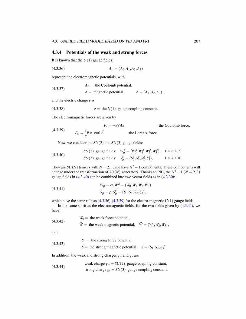
4.3. UNIFIED FIELD MODEL BASED ON PID AND PRI 207
4.3.4 Potentials of the weak and strong forces
It is known that the U(1) gauge fields
(4.3.36) Aµ = (A0,A1,A2,A3)
represent the electromagnetic potentials, with
(4.3.37)A0 = the Coulomb potential,
~A = magnetic potential, ~A = (A1,A2,A3),
and the electric charge e is
(4.3.38) e = the U(1) gauge coupling constant.
The electromagnetic forces are given by
(4.3.39)Fe =−e∇A0 the Coulomb force,
Fm =e
c~v× curl ~A the Lorentz force.
Now, we consider the SU(2) and SU(3) gauge fields:
(4.3.40)SU(2) gauge fields: W a
µ = (W a0 ,W
a1 ,W
a2 ,W
a3 ), 1 ≤ a ≤ 3,
SU(3) gauge fields: Skµ = (Sk
0,Sk1,S
k2,S
k3), 1 ≤ k ≤ 8.
They are SU(N) tensors with N = 2,3, and have N2 −1 components. These components will
change under the transformation of SU(N) generators. Thanks to PRI, the N2 − 1 (N = 2,3)gauge fields in (4.3.40) can be combined into two vector fields as in (4.3.30):
(4.3.41)Wµ = ωaW a
µ = (W0,W1,W2,W3),
Sµ = ρkSkµ = (S0,S1,S2,S3),
which have the same role as (4.3.36)-(4.3.39) for the electro-magnetic U(1) gauge fields.
In the same spirit as the electromagnetic fields, for the two fields given by (4.3.41), we
have
(4.3.42)W0 = the weak force potential,
~W = the weak magnetic potential, ~W = (W1,W2,W3),
and
(4.3.43)S0 = the strong force potential,
~S = the strong magnetic potential, ~S = (S1,S2,S3).
In addition, the weak and strong charges gw and gs are
(4.3.44)weak charge gw = SU(2) gauge coupling constant,
strong charge gs = SU(3) gauge coupling constant.
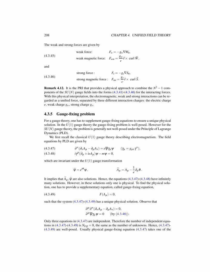
208 CHAPTER 4. UNIFIED FIELD THEORY
The weak and strong forces are given by
(4.3.45)weak force: Fw =−gw∇W0,
weak magnetic force: Fwm =gw
c~v× curl ~W ,
and
(4.3.46)strong force : Fs =−gs∇S0,
strong magnetic force : Fsm =gs
c~v× curl ~S.
Remark 4.12. It is the PRI that provides a physical approach to combine the N2 − 1 com-
ponents of the SU(N) gauge fields into the forms (4.3.41)-(4.3.46) for the interacting forces.
With this physical interpretation, the electromagnetic, weak and strong interactions can be re-
garded as a unified force, separated by three different interaction charges: the electric charge
e, weak charge gw, strong charge gs.
4.3.5 Gauge-fixing problem
For a gauge theory, one has to supplement gauge-fixing equations to ensure a unique physical
solution. In the U(1) gauge theory the gauge-fixing problem is well-posed. However for the
SU(N) gauge theory, the problem is generally not well-posed under the Principle of Lagrange
Dynamics (PLD).
We first recall the classical U(1) gauge theory describing electromagnetism. The field
equations by PLD are given by
∂ ν (∂νAµ − ∂µAν) = eψγµ ψ (γµ = gµνγν ),(4.3.47)
iγµ(∂µ + ieAµ)ψ −mψ = 0,(4.3.48)
which are invariant under the U(1) gauge transformation
ψ = eiθ ψ , Aµ = Aµ −1
e∂µθ .
It implies that Aµ , ψ are also solutions. Hence, the equations (4.3.47)-(4.3.48) have infinitely
many solutions. However, in these solutions only one is physical. To find the physical solu-
tion, one has to provide a supplementary equation, called gauge-fixing equation,
(4.3.49) F(Aµ) = 0,
such that the system (4.3.47)-(4.3.49) has a unique physical solution. Observe that
∂ µ ∂ ν(∂ν Aµ − ∂µAν) = 0,
∂ µ ψγµψ = 0 (by (4.3.48)).
Only three equations in (4.3.47) are independent. Therefore the number of independent equa-
tions in (4.3.47)-(4.3.49) is NEQ = 8, the same as the number of unknowns. Hence, (4.3.47)-
(4.3.49) are well-posed. Usually physical gauge-fixing equation (4.3.47) takes one of the
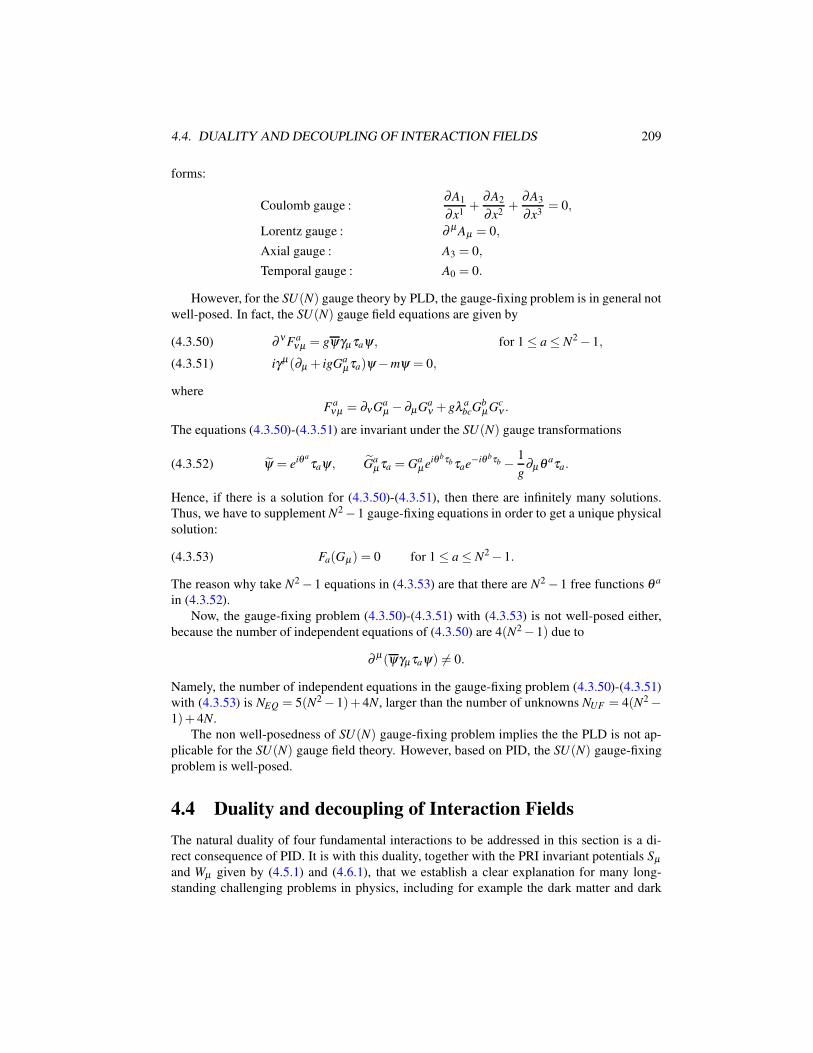
4.4. DUALITY AND DECOUPLING OF INTERACTION FIELDS 209
forms:
Coulomb gauge :∂A1
∂x1+
∂A2
∂x2+
∂A3
∂x3= 0,
Lorentz gauge : ∂ µ Aµ = 0,
Axial gauge : A3 = 0,
Temporal gauge : A0 = 0.
However, for the SU(N) gauge theory by PLD, the gauge-fixing problem is in general not
well-posed. In fact, the SU(N) gauge field equations are given by
∂ ν Faνµ = gψγµ τaψ , for 1 ≤ a ≤ N2 − 1,(4.3.50)
iγµ(∂µ + igGaµτa)ψ −mψ = 0,(4.3.51)
where
Faνµ = ∂νGa
µ − ∂µGaν + gλ a
bcGbµGc
ν .
The equations (4.3.50)-(4.3.51) are invariant under the SU(N) gauge transformations
(4.3.52) ψ = eiθ a
τaψ , Gaµτa = Ga
µeiθ bτbτae−iθ bτb − 1
g∂µ θ aτa.
Hence, if there is a solution for (4.3.50)-(4.3.51), then there are infinitely many solutions.
Thus, we have to supplement N2 −1 gauge-fixing equations in order to get a unique physical
solution:
(4.3.53) Fa(Gµ) = 0 for 1 ≤ a ≤ N2 − 1.
The reason why take N2 − 1 equations in (4.3.53) are that there are N2 − 1 free functions θ a
in (4.3.52).
Now, the gauge-fixing problem (4.3.50)-(4.3.51) with (4.3.53) is not well-posed either,
because the number of independent equations of (4.3.50) are 4(N2 − 1) due to
∂ µ(ψγµτaψ) 6= 0.
Namely, the number of independent equations in the gauge-fixing problem (4.3.50)-(4.3.51)
with (4.3.53) is NEQ = 5(N2 − 1)+ 4N, larger than the number of unknowns NUF = 4(N2 −1)+ 4N.
The non well-posedness of SU(N) gauge-fixing problem implies the the PLD is not ap-
plicable for the SU(N) gauge field theory. However, based on PID, the SU(N) gauge-fixing
problem is well-posed.
4.4 Duality and decoupling of Interaction Fields
The natural duality of four fundamental interactions to be addressed in this section is a di-
rect consequence of PID. It is with this duality, together with the PRI invariant potentials Sµ
and Wµ given by (4.5.1) and (4.6.1), that we establish a clear explanation for many long-
standing challenging problems in physics, including for example the dark matter and dark
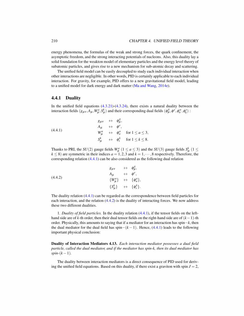
210 CHAPTER 4. UNIFIED FIELD THEORY
energy phenomena, the formulas of the weak and strong forces, the quark confinement, the
asymptotic freedom, and the strong interacting potentials of nucleons. Also, this duality lay a
solid foundation for the weakton model of elementary particles and the energy level theory of
subatomic particles, and gives rise to a new mechanism for sub-atomic decay and scattering.
The unified field model can be easily decoupled to study each individual interaction when
other interactions are negligible. In other words, PID is certainly applicable to each individual
interaction. For gravity, for example, PID offers to a new gravitational field model, leading
to a unified model for dark energy and dark matter (Ma and Wang, 2014e).
4.4.1 Duality
In the unified field equations (4.3.21)-(4.3.24), there exists a natural duality between the
interaction fields (gµν ,Aµ ,Waµ ,S
kµ) and their corresponding dual fields (φ
gµ ,φ
e,φwa ,φ
sk ) :
(4.4.1)
gµν ↔ φgµ ,
Aµ ↔ φ e,
W aµ ↔ φa
w for 1 ≤ a ≤ 3,
Skµ ↔ φ k
s for 1 ≤ k ≤ 8.
Thanks to PRI, the SU(2) gauge fields W aµ (1 ≤ a ≤ 3) and the SU(3) gauge fields Sk
µ (1 ≤k ≤ 8) are symmetric in their indices a = 1,2,3 and k = 1, · · · ,8 respectively. Therefore, the
corresponding relation (4.4.1) can be also considered as the following dual relation
(4.4.2)
gµν ↔ φgµ ,
Aµ ↔ φ e,
W aµ ↔ φa
w,Sk
µ ↔ φ ks .
The duality relation (4.4.1) can be regarded as the correspondence between field particles for
each interaction, and the relation (4.4.2) is the duality of interacting forces. We now address
these two different dualities.
1. Duality of field particles. In the duality relation (4.4.1), if the tensor fields on the left-
hand side are of k-th order, then their dual tensor fields on the right-hand side are of (k−1)-thorder. Physically, this amounts to saying that if a mediator for an interaction has spin−k, then
the dual mediator for the dual field has spin−(k− 1). Hence, (4.4.1) leads to the following
important physical conclusion:
Duality of Interaction Mediators 4.13. Each interaction mediator possesses a dual field
particle, called the dual mediator, and if the mediator has spin-k, then its dual mediator has
spin-(k− 1).
The duality between interaction mediators is a direct consequence of PID used for deriv-
ing the unified field equations. Based on this duality, if there exist a graviton with spin J = 2,
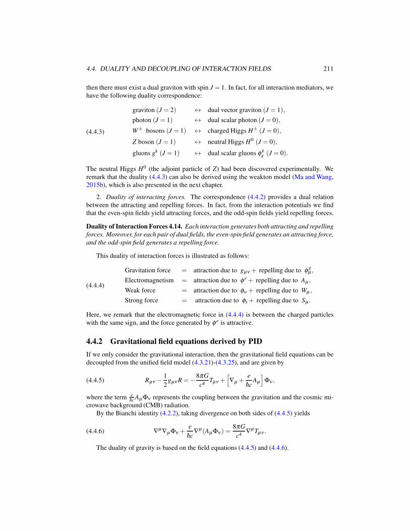
4.4. DUALITY AND DECOUPLING OF INTERACTION FIELDS 211
then there must exist a dual graviton with spin J = 1. In fact, for all interaction mediators, we
have the following duality correspondence:
(4.4.3)
graviton (J = 2) ↔ dual vector graviton (J = 1),
photon (J = 1) ↔ dual scalar photon (J = 0),
W± bosons (J = 1) ↔ charged Higgs H± (J = 0),
Z boson (J = 1) ↔ neutral Higgs H0 (J = 0),
gluons gk (J = 1) ↔ dual scalar gluons φ kg (J = 0).
The neutral Higgs H0 (the adjoint particle of Z) had been discovered experimentally. We
remark that the duality (4.4.3) can also be derived using the weakton model (Ma and Wang,
2015b), which is also presented in the next chapter.
2. Duality of interacting forces. The correspondence (4.4.2) provides a dual relation
between the attracting and repelling forces. In fact, from the interaction potentials we find
that the even-spin fields yield attracting forces, and the odd-spin fields yield repelling forces.
Duality of Interaction Forces 4.14. Each interaction generates both attracting and repelling
forces. Moreover, for each pair of dual fields, the even-spin field generates an attracting force,
and the odd-spin field generates a repelling force.
This duality of interaction forces is illustrated as follows:
(4.4.4)
Gravitation force = attraction due to gµν + repelling due to φgµ ,
Electromagnetism = attraction due to φ e + repelling due to Aµ ,
Weak force = attraction due to φw + repelling due to Wµ ,
Strong force = attraction due to φs + repelling due to Sµ .
Here, we remark that the electromagnetic force in (4.4.4) is between the charged particles
with the same sign, and the force generated by φ e is attractive.
4.4.2 Gravitational field equations derived by PID
If we only consider the gravitational interaction, then the gravitational field equations can be
decoupled from the unified field model (4.3.21)-(4.3.25), and are given by
(4.4.5) Rµν −1
2gµνR =−8πG
c4Tµν +
[∇µ +
e
hcAµ
]Φν ,
where the term ehc
AµΦν represents the coupling between the gravitation and the cosmic mi-
crowave background (CMB) radiation.
By the Bianchi identity (4.2.2), taking divergence on both sides of (4.4.5) yields
(4.4.6) ∇µ ∇µΦν +e
hc∇µ(AµΦν ) =
8πG
c4∇µTµν .
The duality of gravity is based on the field equations (4.4.5) and (4.4.6).
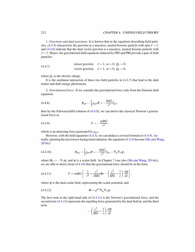
212 CHAPTER 4. UNIFIED FIELD THEORY
1. Gravitons and dual gravitons. It is known that as the equations describing field parti-
cles, (4.4.5) characterize the graviton as a massless, neutral bosonic particle with spin J = 2,
and (4.4.6) indicate that the dual vector graviton is a massless, neutral bosonic particle with
J = 1. Hence, the gravitational field equations induced by PID and PRI provide a pair of field
particles:
(4.4.7)tensor graviton: J = 2, m = 0, Qe = 0,
vector graviton: J = 1, m = 0, Qe = 0,
where Qe is the electric charge.
It is the nonlinear interaction of these two field particles in (4.4.7) that lead to the dark
matter and dark energy phenomena.
2. Gravitational force. If we consider the gravitational force only from the Einstein field
equations
(4.4.8) Rµν −1
2gµνR =−8πG
c4Tµν ,
then by the Schwarzschild solution of (4.4.8), we can derive the classical Newton’s gravita-
tional force as
(4.4.9) F =−mMG
r2,
which is an attracting force generated by gµν .
However, with the field equations (4.4.5), we can deduce a revised formula to (4.4.9). Ac-
tually, ignoring the microwave background radiation, the equations (4.4.5) become (Ma and Wang,
2014e):
(4.4.10) Rµν −1
2gµνR =−8πG
c4Tµν −∇µ∇νϕ ,
where Φν = −∇νϕ , and ϕ is a scalar field. In Chapter 7 (see also (Ma and Wang, 2014e)),
we are able to derive from (4.4.10) that the gravitational force should be in the form
(4.4.11) F = mMG
[− 1
r2+
c2
2MGΦr−
(c2
MG+
1
r
)dϕ
dr
],
where ϕ is the dual scalar field, representing the scalar potential, and
(4.4.12) Φ = gµν∇µ∇ν ϕ .
The first term in the right-hand side of (4.4.11) is the Newton’s gravitational force, and the
second term (4.4.12) represents the repelling force generated by the dual field ϕ , and the third
term
−(
c2
MG+
1
r
)dϕ
dr
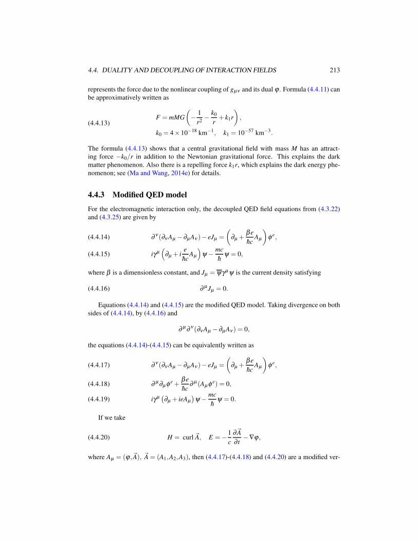
4.4. DUALITY AND DECOUPLING OF INTERACTION FIELDS 213
represents the force due to the nonlinear coupling of gµν and its dual ϕ . Formula (4.4.11) can
be approximatively written as
(4.4.13)F = mMG
(− 1
r2− k0
r+ k1r
),
k0 = 4× 10⁻¹⁸ km−1, k1 = 10−57 km−3.
The formula (4.4.13) shows that a central gravitational field with mass M has an attract-
ing force −k0/r in addition to the Newtonian gravitational force. This explains the dark
matter phenomenon. Also there is a repelling force k1r, which explains the dark energy phe-
nomenon; see (Ma and Wang, 2014e) for details.
4.4.3 Modified QED model
For the electromagnetic interaction only, the decoupled QED field equations from (4.3.22)
and (4.3.25) are given by
∂ ν(∂ν Aµ − ∂µAν)− eJµ =
(∂µ +
β e
hcAµ
)φ e,(4.4.14)
iγµ(
∂µ + ie
hcAµ
)ψ − mc
hψ = 0,(4.4.15)
where β is a dimensionless constant, and Jµ = ψγµψ is the current density satisfying
(4.4.16) ∂ µJµ = 0.
Equations (4.4.14) and (4.4.15) are the modified QED model. Taking divergence on both
sides of (4.4.14), by (4.4.16) and
∂ µ∂ ν (∂νAµ − ∂µAν) = 0,
the equations (4.4.14)-(4.4.15) can be equivalently written as
∂ ν(∂ν Aµ − ∂µAν)− eJµ =
(∂µ +
β e
hcAµ
)φ e,(4.4.17)
∂ µ∂µφ e +β e
hc∂ µ(Aµφ e) = 0,(4.4.18)
iγµ(∂µ + ieAµ
)ψ − mc
hψ = 0.(4.4.19)
If we take
(4.4.20) H = curl ~A, E =−1
c
∂~A
∂ t−∇ϕ ,
where Aµ = (ϕ ,~A), ~A = (A1,A2,A3), then (4.4.17)-(4.4.18) and (4.4.20) are a modified ver-
214 CHAPTER 4. UNIFIED FIELD THEORY
sion of the classical Maxwell equations, which are expressed as
(4.4.21)
1
c
∂H
∂ t=− curl E,
H = curl ~A,
1
c
∂E
∂ t= curl H + ~J+∇φ e +
β e
hcAµφ e,
div E = ρ +1
c
∂φ e
∂ t+
β e
hcφ eϕ ,
(∂ 2
∂ t2−∆
)φ e +
β e
hc
(1
c
∂
∂ t(ϕφ e)− div (~Aφ e)
)= 0,
where ~J is the electric current density and ρ is the electric charge density.
The equations (4.4.14)-(4.4.15) or (4.4.17)-(4.4.19) need to be supplemented with a cou-
pled equation to compensate the gauge-symmetry breaking and the induced dual field φ e:
(4.4.22) F(Aµ ,φe,ψ) = 0.
Remark 4.15. Usually, the compensating equation (4.4.22) is called the gauge-fixing equa-
tion. The compensating equation (4.4.22) should be determined based on first principles.
However, we don’t know whether there are such physical laws. In general, according to
different situations physicists take the gauge-fixing equation in the following forms:
(4.4.23)
Lorentz gauge: ∂ µAµ = 0,
Coulomb gauge: div ~A = 0,
Axial gauge: A3 = 0,
Temporal gauge: A0 = 0 (A0 = ϕ).
The following are the two perspectives of the duality for electromagnetism.
1. Photon and dual scalar photon. If we view the field equations (4.4.17) and (4.4.18) as
describing the field particles, then we have
Jµ = 0, β = 0 in (4.4.17)-(4.4.18).
Thus, the usual photon equation is given by
(4.4.24) Aµ + ∂µ(∂ν Aν) = 0,
and the dual photon, also called the scalar photon, is described by the following equation
(4.4.25) φ e = 0.
By (4.4.24) and (4.4.25) we deduce the following basic properties for photons and scalar
photons:
(4.4.26)photon: J = 1, m = 0, Qe = 0,
scalar photon: J = 0, m = 0, Qe = 0.
4.4. DUALITY AND DECOUPLING OF INTERACTION FIELDS 215
2. Electromagnetic force. If we consider the electromagnetic force, then the constant
β 6= 0 in (4.4.17). It is known that in the classical theory, the Coulomb potential ϕ satisfies
the equation
(4.4.27) ∆ϕ =−4πρ ,
which is the stationary equation of (4.4.17) with µ = 0 and Φe = 0, and with the Coulomb
gauge in (4.4.23). For the case where ρ = eδ (r), the solution of (4.4.27) is the well-known
Coulomb potential:
(4.4.28) ϕ =e
r.
For the modified equations (4.4.17) and (4.4.18), the stationary time-component equations
with the Coulomb gauge are given by
∆ϕ − β e
hcφ eϕ = 4πeδ (r)(4.4.29)
∆φ e = 0.(4.4.30)
Only the radially symmetric solutions of (4.4.29) and (4.4.30) are physical. The radial solu-
tions of (4.4.30) are constants
φ e = φ0 the constants.
Thus the equations (4.4.29) and (4.4.30), in the spherical coordinate system, are reduced as
follows
(4.4.31)1
r2
d
dr(r2 d
dr)ϕ − kϕ =−4πeδ (r),
where k = ehc
β φ0. The solutions of (4.4.31) are expressed as
(4.4.32) ϕ =e
re−
√kr.
The parameter k is to be determined by experiments.
We discuss the solutions (4.4.32) in the following three cases.
1) Case k = 0. The solution (4.4.32) in this case is reduced to the Coulomb potential
(4.4.28);
2) Case k > 0. This solution is similar to the Yukawa potential for the strong interactions
of nucleons.
3) Case k < 0. In this case, the solution can be written as
(4.4.33) ϕ =e
rcos
√−kr+
αe
rsin
√−kr,
where α is an arbitrary constant. The function
ϕ0 =1
rsin
√−kr
in (4.4.33) satisfies that
∆ϕ0 − kϕ0 = 0.
216 CHAPTER 4. UNIFIED FIELD THEORY
4.4.4 Strong interaction field equations
The decoupled strong interaction field model from (4.3.21)-(4.3.25) is given by
∂ ν Skνµ −
gs
hcf ki jg
αβ SiαµS
j
β− gsQ
kµ =
[∂µ +
gs
hcδ s
l Slµ −
1
4
(mπ c
h
)2
xµ
]φ k
s ,(4.4.34)
iγµ[∂µ + i
gs
hcSb
µτb
]ψ − mc
hψ = 0,(4.4.35)
for 1 ≤ k ≤ 8, where τk = τk are the Gell-Mann matrices as in (3.5.38), and
(4.4.36)Sk
µν = ∂µSkν − ∂νSk
µ +gs
hcSi
µSjν ,
Qkµ = ψγµτkψ .
Taking divergence on both sides of (4.4.34) and by
∂ µ ∂ νSkµν = 0 for 1 ≤ k ≤ 8,
we deduce the following dual field equations for the strong interaction:
∂ µ ∂µφ ks + ∂ µ
[(gs
hcδ k
l Slµ −
1
4
m2π c2
h2xµ
)φ k
s
]=−gs∂
µQkµ − gs
hcf ki jg
αβ ∂ µ(SiαµS
j
β).(4.4.37)
The equations (4.4.34)-(4.4.35) also need 8 additional gauge equations to compensate the
induced dual fields φ ks :
(4.4.38) Fks (Sµ ,φs,ψ) = 0, 1 ≤ k ≤ 8.
We have the following duality for the strong interaction.
1. Gluons and dual scalar gluons. Based on quantum chromodynamics (QCD), the
field particles for the strong interaction are the eight massless gluons with spin J = 1, which
are described by the SU(3) gauge fields Skµ (1 ≤ k ≤ 8). By the duality (4.4.1), for the strong
interactions we have the field particle correspondence
Skµ ↔ φ k
s for 1 ≤ k ≤ 8.
It implies that corresponding to the 8 gluons Skµ (1 ≤ k ≤ 8) there should be 8 dual gluons
represented by φ ks , called the scalar gluons due to φ k
s being scalar fields. Namely we have the
following gluon correspondence
gluons gk ↔ scalar gluons gk0 for 1 ≤ k ≤ 8.
Gluons and scalar gluons are described by equations (4.4.34) and (4.4.37) respectively,
which are nonlinear. In fact, gk and gk0 are confined in hadrons.
4.4. DUALITY AND DECOUPLING OF INTERACTION FIELDS 217
2. Strong force. The strong interaction forces are governed by the field equations
(4.3.31)-(4.3.35). The decoupled field equations are given by
∂ νSkνµ − gs
hcf ki jg
αβ SiαµS
j
β− gsQ
kµ =
[∂µ − 1
4k2
s xµ +gsδ
hcSµ
]φ k
s ,(4.4.39)
∂ µ∂µφ ks − k2φ k
s +1
4k2
s xµ∂ µ φ ks +
gsδ
hc∂ µ(Sµφ k
s )(4.4.40)
=−gs∂µ Qk
µ −gs
hcf ki jg
αβ ∂ µ(SiαµS
j
β ),
iγµ[∂µ + i
gs
hcSl
µτl
]ψ − mc
hψ = 0,(4.4.41)
for 1 ≤ k ≤ 8, where δ is a parameter,and Sµ is as in (4.3.41).
In the next section, we shall deduce the layeredformulas of strong interaction potentials
from the equations (4.4.39)-(4.4.41) with gauge equations (4.4.38).
Remark 4.16. We need to explain the physical significance of the parameters ks and δ .
Usually, ks and δ are regarded as masses of the field particles. However, since (4.4.39)-
(4.4.41) are the field equations for the interaction forces, the parameters ks and δ are no
longer viewed as masses. In fact, k−1 represents the range of attracting force for the strong
interaction, and(
gsφ 0s
hcδ)−1
is the range of the repelling force, where φ0s is a ground state of
φs.
4.4.5 Weak interaction field equations
The unified field model (4.3.21)-(4.3.25) can be decoupled to study the weak interaction only,
leading to the following weak interaction field equations:
∂ νW aνµ − gw
hcεa
bcgαβW bαµW c
β − gwJaµ =
[∂µ − 1
4
(mHc
h
)2
xµ +gw
hcγw
b W bµ
]φa
w,(4.4.42)
iγµ[∂µ + i
gw
hcW a
µ σa
]ψ − mc
hψ = 0,(4.4.43)
where mH represents the mass of the Higgs particle, σa = σa (1 ≤ a ≤ 3) are the Pauli
matrices as in (3.5.36), and
(4.4.44)W a
µν = ∂µW aν − ∂νW a
µ +gw
hcεa
bcWbµW c
ν ,
Jaµ = ψγµσaψ , γµ = gµνγν .
Taking divergence on both sides of (4.4.42) we get
∂ µ ∂µφaw −
(mHc
h
)2
φaw +
gw
hcγw
b ∂ µ(W bµ φa
w)−1
4(
mHc
h)2xµ∂ µφa
w(4.4.45)
=−gw
hcεa
bcgαβ ∂ µ(W bαµW c
β )− gw∂ µ Jaµ .
Also, we need to supplement (4.4.42)-(4.4.43) with three additional 3 gauge equations to
compensate the induced dual fields φaw:
(4.4.46) Faw(Wµ ,φw,ψ) = 0 for 1 ≤ a ≤ 3.
218 CHAPTER 4. UNIFIED FIELD THEORY
1. Duality between W±,Z Bosons and Higgs Bosons H±,H0. The three massive vector
bosons, denoted by W±,Z0, has been discovered experimentally. The field equations (4.4.42)
give rise to a natural duality:
(4.4.47) Z0 ↔ H0, W± ↔ H±,
where H0,H± are three dual scalar bosons, called the Higgs particles. The neutral Higgs H0,
discovered by LHC in 2012, and the charged Higgs H±, to be discovered experimentally.
In Section 4.6, we shall introduce the dual bosons (4.4.47) by applying the field equations
(4.4.42)-(4.4.45) with gauge equations (4.4.46).
2. Weak force. If we consider the weak interaction force, we have to use the equations
decoupled from (4.3.31)-(4.3.35):
∂ νW aνµ − gw
hcεa
bcgαβW bαµW c
β − gwJaµ =
[∂µ −
1
4k2
wxµ +gw
hcγWµ
]φa
w,(4.4.48)
∂ µ ∂µφaw − k2φ2
w +gw
hcγ∂ µ(Wµφa
w)−1
4k2xµ∂ µ φa
w(4.4.49)
=−gw∂ µJaµ − gw
hcεa
bcgαβ ∂ µ(W bαµW c
β ),
iγµ(∂µ + igw
hcW a
µ σa)ψ − mc
hψ = 0,(4.4.50)
where γ,kw are constants, Wµ is as in (4.3.41).
In Section 4.6, we shall deduce the layered formulas of weak interaction potentials by
applying the equations (4.4.48)-(4.4.50).
Remark 4.17. The duality of four fundamental interactions is very important, and is a direct
consequence of PID. With this duality, and with the PRI invariant potentials Wµ and Sµ given
by (4.3.41), we obtain explanations for a number of physical problems such as the dark matter
and dark energy phenomena, the weak and strong forces and potential formulas, the quark
confinement, the asymptotic freedom, the strong potentials of nucleons etc. Also this study
leads to the needed foundation for the weakton model of elementary particles and the energy
level theory of subatomic particles, and gives rise to a mechanism for subatomic decays and
scatterings.
4.5 Strong Interaction Potentials
4.5.1 Strong interaction potential of elementary particles
Thanks to PRI, the strong interaction potential takes the linear combination of the eight SU(3)gauge potentials as follows
(4.5.1) Sµ = ρkSkµ ,
where ρk = (ρ1, · · · ,ρ8) is the SU(3) tensor as given in (4.3.29).
Let gs be the strong charge of an elementary particle, i.e. the w∗ weakton introduced in
Chapter 5, and
Φ0 = S0 the time-component of (4.5.1)
4.5. STRONG INTERACTION POTENTIALS 219
be the strong charge potential of this particle. Then the strong force between two elementary
particles carrying strong charges is
F =−gs∇Φ0.
However, the strong interactions are layered, i.e. the strong forces only act on the same
level of particles, such as the quark level, the hadron level. Hence, the strong interaction
potentials are also layered. In fact, in the next subsection we shall show that for a particle
with N strong charges gs of the elementary particles, its strong interaction potential is given
by
(4.5.2)
Φs = Ngs(ρ)
[1
r− A
ρ(1+ kr)e−kr
],
gs(ρ) =
(ρw
ρ
)3
gs,
where ρw is the radius of the elementary particle (i.e. the w∗ weakton), ρ is the particle radius,
k > 0 is a constant with k−1 being the strong interaction attraction radius of this particle, and
A is the strong interaction constant, which depends on the type of particles. Thus, the strong
force between such two particles is
(4.5.3) F =−Ngs(ρ)∇Φs,
where gs(ρ) and Φs are as in (4.5.2).
In particular for the w∗-weakton, which possesses one strong charge gs, the formula
(4.5.2) becomes
(4.5.4) Φ0 = gs
[1
r− A0
ρw
(1+ k0r)e−k0r
],
where 1/k0 is the attraction radius of the strong interaction for the elementary particles, i.e.
the w∗-weakton. According to the physical observation, we take the quantitative order
(4.5.5) k0 = 1018 cm−1.
In this subsection, we shall deduce formula (4.5.4) for the w∗-weaktons from the strong
interaction field equations (4.4.39)-(4.4.41). Taking inner product of the field equation (4.4.39)
and (4.4.40) with ρk = (ρ1, · · · ,ρ8), we derive that
∂ ν Sνµ −gs
hcλi jg
αβ SiαµS
j
β− gsQµ =
[∂µ − 1
4k2
0xµ +gsδ
hcSµ
]φs,(4.5.6)
(1
c2
∂ 2
∂ t2−∆
)φs + k2
0φs +1
4k2
0xµ∂ µ φs(4.5.7)
= gs∂µ Qµ +
gs
hc∂ µ(λi jg
αβ SiαµS
j
β − δSµφs),
220 CHAPTER 4. UNIFIED FIELD THEORY
where
φs = ρkφ ks , Qµ = ρkQk
µ , λi j = ρkλ ki j, Sµν = ∂µSν − ∂νSµ +
gs
hcλi jS
iµS
jν .
Based on the superposition property of the strong potential for strong charges, Φs = S0
and φs obey a linear relationship. Namely, the time-component µ = 0 equation of (4.5.6)
and the equation (4.5.7) should be linear. In other words, we have to take eight gauge fixing
equations as in (4.4.38) such that they contain the following two equations:
(4.5.8)λi j
[∂ ν(Si
νSj0)− gαβ Si
αoSj
β
]+ δS0φs = 0,
∂ µ[λi jg
αβ Siαβ S
j
β− δSµφs
]= 0,
Also, in the eight supplement equations we take
(4.5.9) xµ∂ µφs = 0, ∂ µSµ = 0,
together with the following static assumption:
(4.5.10)∂S0
∂ t= 0,
∂φs
∂ t= 0.
With the gauge fixing equations (4.5.8)-(4.5.9) and the static assumption (4.5.10), we
derive from (4.5.6) and (4.5.7) that
−∆Φs = gsQ− 1
4k2
0cτφs,(4.5.11)
−∆φs + k20φs = gs∂
µQµ ,(4.5.12)
where cτ is the wave length of φs,Q =−Q0.
In the following, we deduce the solution Φs and φs of (4.5.11)-(4.5.12) in a few steps.
Step 1. Solution of (4.5.12). By definition of Qµ , we have
∂ µ Qµ = ρk∂µψγµτkψ +ρkψγµτk∂µψ .
In view of the Dirac equation (4.4.41),
∂µ ψγµ τkψ = igs
hcS
jµψγµτ jτkψ + i
mc
hψτkψ ,
ψγµτk∂µψ =−igs
hcS
jµψγµτkτ jψ − i
mc
hψτkψ .
Hence we arrive at
(4.5.13) ∂ µ Qµ =igs
hcρkS
jµψγµ [τ j,τk]ψ =−2gs
hcρkS
jµλ i
jkQµi
Since Qµi = Qi
µ is the current density, we have
ρkλ ijkQ
µi = θ
µj δ (r),
4.5. STRONG INTERACTION POTENTIALS 221
where δ (r) is the Dirac delta function, θµj is a constant tensor, inversely proportional to the
volume of the particle. Hence
ρkSjµλ i
jkθµi = S
j
µθµj δ (r),
where Sj
µ ∼ Sj
µ(0) takes the following average value
(4.5.14) Sj
µ =1
|Bρw |
∫
Bρw
Sjµdv.
Here ρw is the radius of a w∗-weakton. Later, we shall see that
Sjµ ∼ 1
ras r → 0.
Hence we deduce from (4.5.14) that
Sj
µ = ξ jµρ−1
w (ξ jµ is a constant tensor).
Thus, (4.5.13) becomes
(4.5.15) ∂ µ Qµ =− κ
ρw
δ (r) (ρw is the radius of a w∗-weakton),
where κ is a parameter given by
(4.5.16) κ =2gs
hcξ
jµθ
µj ,
and κ is inversely proportional to the volume of w∗-weakton.
Therefore, equation (4.5.12) is rewritten as
(4.5.17) −∆φs + k20φs =−gsκ
ρw
δ (r),
whose solution is given by
(4.5.18) φs =−gsκ
ρw
1
re−k0r.
Step 2. Solution of (4.5.11). The quantity gsQ = −gsQ0 is the strong charge density of a
w∗-weakton, and without loss of generality, we assume that
(4.5.19) Q = β δ (r),
and β > 0 is a constant, inversely proportional to the volume of the w∗-weakton. Hence
(4.5.11) can be rewritten as
(4.5.20) −∆Φs = gsβ δ (r)+gsA
ρw
1
re−k0r,
222 CHAPTER 4. UNIFIED FIELD THEORY
where A is a constant given by
A =k2
0cτκ
4with physical dimension
1
L.
Assume Φs = Φs(r) is radially symmetric, then (4.5.20) becomes
− 1
r2
d
dr(r2 d
dr)Φs = gsβ δ (r)+
gsA
ρw
1
re−k0r,
whose solution takes the form
(4.5.21) Φs = gs
[β
r− A
ρw
ϕ(r)e−k0r
],
where ϕ solves
(4.5.22) ϕ ′′+ 2
(1
r− k0
)ϕ ′−
(2k0
r− k2
0
)ϕ =
1
r.
Assume that the solution ϕ of (4.5.22) is given by
(4.5.23) ϕ =∞
∑k=0
αkrk.
Inserting ϕ in (4.5.22) and comparing the coefficients of rk, then we obtain the following
relations
α1 = k0α0 +1
2,
α2 =1
2k2
0α0 +1
3k0,
...(4.5.24)
αk =2k0
k+ 1αk−1 − k2
0αk−2, ∀k ≥ 2.
where α0 is a free parameter with dimension L. Hence
ϕ(r) = α0(1+ k0r+r
2α0
+ o(r)),
and often it is sufficient to take a first-order approximation.
Step 3. Strong interaction potential of w∗-weakton. The formula (4.5.21) with (4.5.23)-
(4.5.24) provides an accurate strong interaction potential for the w∗-weaktons:
(4.5.25) Φ0 = gsβ
[1
r− A0
ρw
ϕ(r)e−k0r
],
where A0 = Aα0/β is a dimensionless parameter, and ϕ(r) is
ϕ = 1+ k0r+r
2α0
+ o(r),
4.5. STRONG INTERACTION POTENTIALS 223
which is a dimensionless function, and
(4.5.26) β is inversely proportional to the particle volume.
Since gsβ is to be determined for the elementary particle, we can take gsβ as the strong
charge of the w∗-weakton, still denoted by gs. In addition, it is sufficient to take approxima-
tively ϕ = 1+ k0r. Then the formula (4.5.25) is rewritten as
Φ0 = gs
[1
r− A0
ρw
(1+ k0r)e−k0r
].
It is the strong interaction potential given in (4.5.4).
4.5.2 Layered formulas of strong interaction potentials
Different from gravity and electromagnetic force, strong interaction is of short-ranged with
different strengths in different levels. For example, in the quark level, strong interaction con-
fines quarks inside hadrons, in the nucleon level, strong interaction bounds nucleons inside
atoms, and in the atom and molecule level, strong interaction almost diminishes. This layered
phenomena can be well-explained using the unified field theory based on PID and PRI. We
derive in this subsection strong interaction potentials in different levels.
Without loss of generation, we shall discuss strong interaction nucleon potential. For
strong interaction of nucleons, we still use the SU(3) gauge action
(4.5.27) L =−1
4Sk
µνSµνk + hcq(iγµDµ − mc
h)q,
where Skµ are the strong interaction gauge fields,
(4.5.28) q = (q1,q2,q3)
where q1,q2,q3 are the wave functions of the three quarks constituting a nucleon, and
(4.5.29) Dµq = (hc∂µ +igs
hcSk
µτk)q.
The action L defined by (4.5.27) is SU(3) gauge invariant. Physically this means that the
contribution of each quark to the strong interaction potential energy is indistinguishable. With
PID, the corresponding field equations for the action (4.5.27) are
∂ ν Skνµ +
gs
hcλ k
i jgαβ Si
αµSj
β − gsQkµ =
(∂µ − k2
1
4xµ
)φ k
n ,(4.5.30)
iγµ(
∂µ + igs
hcSk
µτk
)q− mc
hq = 0,(4.5.31)
where the parameter k1 is defined by
(4.5.32) r1 =1
k1
= 10−13 cm,
224 CHAPTER 4. UNIFIED FIELD THEORY
which is the strong attraction radius of nucleons, and
Qkµ = qγµ τkq (τk = τk).
Let the strong interaction nucleon potential Φkn and its dual potential φn be defined by
Φn = ρkSk0, φn = ρkφ k
n .
In the same spirit as for deriving the weakton potential equations (4.5.11) and (4.5.12), for
Φn and φn we deduce that
(4.5.33)−∆Φn = gsQn −
1
4k2
1cτ1φn,
−∆φn + k21φn = gs∂
µQµ ,
where cτ1 is the wave length of φn, and
Qµ = ρkQkµ = (Q0,Q1,Q2,Q3)
represents the quark current density inside a nucleon. Similar to (4.5.15) and (4.5.19), for Qn
and ∂ µ Qµ we have
(4.5.34) ∂ µQµ =−κn
ρn
δ (r), Qn = βnδ (r),
where ρn is the radius of a nucleon, βn and κn are constants, inversely proportional to the
volume of nucleons. Hence, in the same fashion as in deducing (4.5.25), from (4.5.33) and
(4.5.34) we derive the following strong nucleon potential as
(4.5.35) Φn = βngs
[1
r− An
ρn
ϕ(r)e−k1r
],
where ϕ(r) is as
(4.5.36) ϕ(r) = 1+ k1r+r
2α0
+ o(r), α0 as in (4.5.24),
and An is a dimensionless parameter:
An =κnk2
1cτ1
4βn
.
Note that βn is inversely proportional to the volume Vn of a nucleon. Hence we have
(4.5.37)βn
β=
NV0
Vn
= N
(ρw
ρn
)3
(N = 3),
where N is the number of strong charges in a nucleon, β is the parameter as in (4.5.25) and
(4.5.26), and V0 the volume of a w∗-weakton. Since gsβ in (4.5.25) is taken as gs, by (4.5.37)
the formula (4.5.35) is expressed as
(4.5.38)
Φn = gs(ρn)
[1
r− An
ρn
ϕ(r)e−knr
],
gs(ρn) = 3
(ρw
ρn
)3
gs,
4.5. STRONG INTERACTION POTENTIALS 225
and ϕ(r) is as in (4.5.36).
In summary, for a particle with N strong charges and radius ρ , its strong interaction
potential can be written as
(4.5.39)
Φ = gs(ρ)
[1
r− A
ρϕ(r)e−kr
],
gs(ρ) = N
(ρw
ρ
)3
gs,
where ρw is the radius of w∗-weakton, A is a dimensionless constant depending on the particle,
ϕ(r) = 1+kr, and 1/k is the radius of strong attraction of particles. Phenomenologically, we
take
(4.5.40)1
k=
10−18 cm for w∗− weaktons,
10−16 cm for quarks,
10−13 cm for neutreons,
10−7 cm for atom/molecule.
More specifically, we give the following layered formulas of strong interaction poten-
tials for various level of particles as the w∗-weakton potential Φ0, the quark potential Φq,
the nucleon/hadron potential Φn and the atom/molecule potential Φa are given as follows
(Ma and Wang, 2014c):
(4.5.41)
Φ0 = gs
[1
r− A0
ρw
(1+ k0r)e−k0r
],
Φq =
(ρw
ρq
)3
gs
[1
r− Aq
ρq
(1+ k1r)e−k1r
],
Φn = 3
(ρw
ρn
)3
gs
[1
r− An
ρn
(1+ knr)e−knr
],
Φa = N
(ρw
ρa
)3
gs
[1
r− Aa
ρa
(1+ kar)e−kar
].
Here, k0,k1,kn,ka are taken as in (4.5.40):
(4.5.42)
1
k0
= 10−18 cm,1
k1
= 10−16 cm,
1
kn= 10−13 cm,
1
ka= 10−10 ∼ 10−7 cm.
Remark 4.18. For two particles with N1,N2 strong charges and radii ρ1,ρ2, their strong
potential energy is
(4.5.43) V = gs(ρ1)gs(ρ2)
[1
r− B
ρ(1+ kr)e−kr
],
where B and k depend on the two types of particles, and ρ depends on ρ1 and ρ2 with ρ = ρif ρ = ρ1 = ρ2. The strong force between the two particles is
(4.5.44) F =−∇V, V as in (4.5.43).
226 CHAPTER 4. UNIFIED FIELD THEORY
4.5.3 Quark confinement
Quark model was confirmed by lots of experiments. However, no any single quark is found
ever. This fact suggests that the quarks were permanently bound inside a hadron, which is
called the quark confinement. Up to now, no other theories can successfully describe the
quark confinement phenomena. The direct reason is that all current theories for interactions
fail to provide a successful strong interaction potential to explain the various level strong
interactions.
Now, we can derive the quark confinement by using the layered strong interaction poten-
tials (4.5.41).
The strong interaction bound energy E for two particles is given by (4.5.43). In particular,
for two same particles we have
(4.5.45)
E = g2s (ρ)
[1
r− A
ρ(1+ kr)e−kr
],
gs(ρ) =
(ρw
ρ
)3
gs.
The quark confinement can be well explained from the viewpoint of the strong quark
bound energy Eq and the nucleon bound energy En. In fact, by (4.5.45) we have
(4.5.46)Eq
En
⋍Aq
An
(ρn
ρq
)7
.
According to the physical observation fact,
(4.5.47) ρn ⋍ 10−16 cm, ρq ⋍ 10−19 cm.
Then, by (4.5.46) we derive thatEq
En
⋍ 1021 Aq
An
.
Physically Aq/An is no small, and we assume that Aq/An ⋍ 10−1. Then we have
(4.5.48) Eq = 1020En.
It is known that the bound energy of nucleons is about
En ∼ 10−2GeV.
Thus, we obtain by (4.5.48) that
Eq ∼ 1018GeV,
which is at the Planck level. This clearly shows that the quarks is confined in hadrons, and
no free quarks can be found.
Remark 4.19. The magnitude order (4.5.42) and (4.5.47) are not accurate, but they are
enough precisely to explain the important physical problems as the quark confinement and
asymptotic freedom etc.
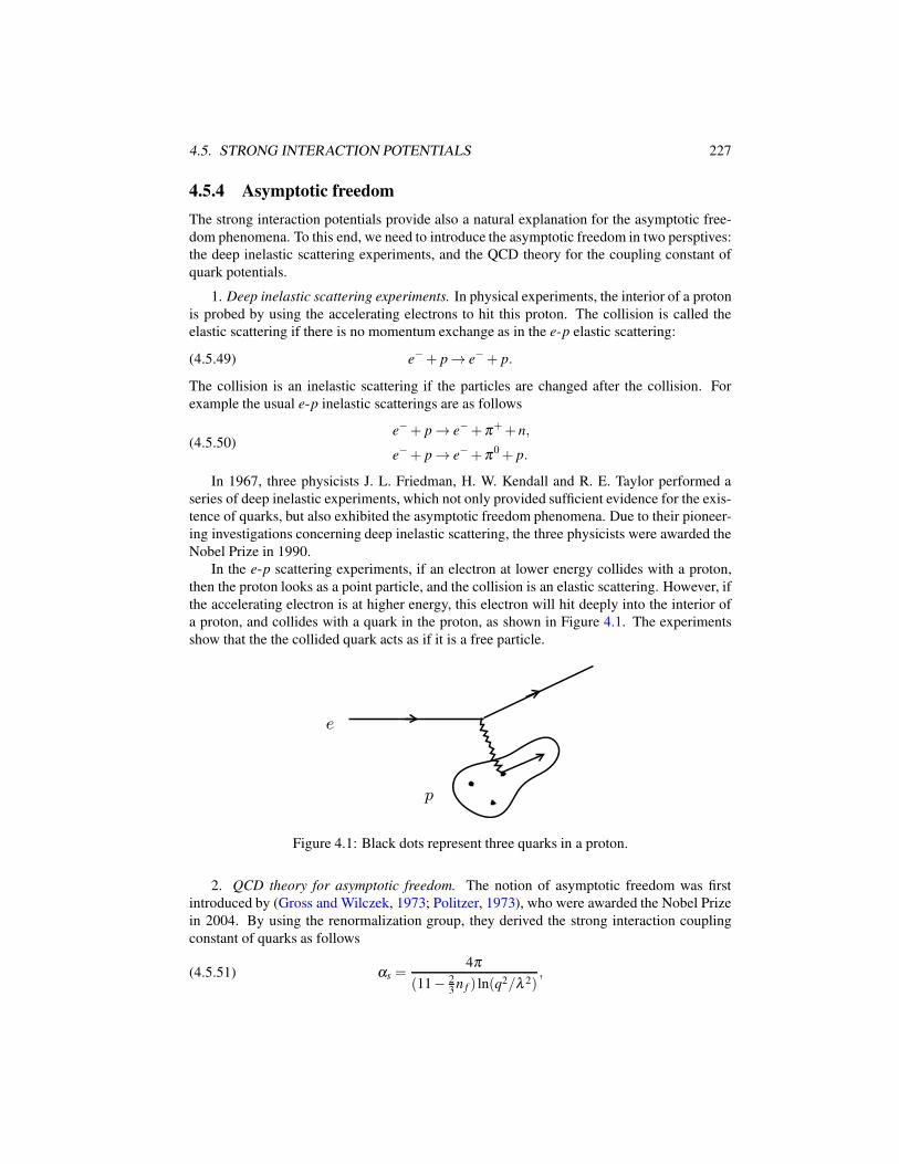
4.5. STRONG INTERACTION POTENTIALS 227
4.5.4 Asymptotic freedom
The strong interaction potentials provide also a natural explanation for the asymptotic free-
dom phenomena. To this end, we need to introduce the asymptotic freedom in two persptives:
the deep inelastic scattering experiments, and the QCD theory for the coupling constant of
quark potentials.
1. Deep inelastic scattering experiments. In physical experiments, the interior of a proton
is probed by using the accelerating electrons to hit this proton. The collision is called the
elastic scattering if there is no momentum exchange as in the e-p elastic scattering:
(4.5.49) e−+ p → e−+ p.
The collision is an inelastic scattering if the particles are changed after the collision. For
example the usual e-p inelastic scatterings are as follows
(4.5.50)e−+ p → e−+π++ n,
e−+ p → e−+π0 + p.
In 1967, three physicists J. L. Friedman, H. W. Kendall and R. E. Taylor performed a
series of deep inelastic experiments, which not only provided sufficient evidence for the exis-
tence of quarks, but also exhibited the asymptotic freedom phenomena. Due to their pioneer-
ing investigations concerning deep inelastic scattering, the three physicists were awarded the
Nobel Prize in 1990.
In the e-p scattering experiments, if an electron at lower energy collides with a proton,
then the proton looks as a point particle, and the collision is an elastic scattering. However, if
the accelerating electron is at higher energy, this electron will hit deeply into the interior of
a proton, and collides with a quark in the proton, as shown in Figure 4.1. The experiments
show that the the collided quark acts as if it is a free particle.
e
p
Figure 4.1: Black dots represent three quarks in a proton.
2. QCD theory for asymptotic freedom. The notion of asymptotic freedom was first
introduced by (Gross and Wilczek, 1973; Politzer, 1973), who were awarded the Nobel Prize
in 2004. By using the renormalization group, they derived the strong interaction coupling
constant of quarks as follows
(4.5.51) αs =4π
(11− 23n f ) ln(q2/λ 2)
,
228 CHAPTER 4. UNIFIED FIELD THEORY
where λ is a parameter, n f = 6 is the flavor number of quarks, and q2 is the transfer momen-
tum by the incidence electron.
In QCD, the coupling constant αs stands for the strength of the strong interactions be-
tween the quarks in a proton. It is clear that as the transfer momentum q2 tends to infinitely
large, αs tends to zero:
(4.5.52) αs → 0 as q2 → ∞.
It means that the greater the incidence electron kinetics is, the more freedom the quarks
exhibit. The asymptotic freedom is based on the fact (4.5.51)-(4.5.52).
3. Strong interaction potential for asymptotic freedom. The strong interaction potentials
provide also a natural explanation for the asymptotic freedom phenomena. By (4.5.41) and
(4.5.44), the strong force between quarks is as
F =−gs(ρq)dΦq
dr= g2
s (ρq)
[1
r2− Aq
ρq
k21re−k1r
],
which implies that there are two radii r1 and r2 such that
ρq < r1 < r1 < r2 (r1 = 1/k1),
and the strong force F satisfies
(4.5.53) F
> 0 for 0 < r < r1,< 0 for r1 < r < r2.
By (4.5.53), we see that
F ∼ 0 near r = r1.
This indicates that there is a free shell region inside a proton with radius R ≃ r1, such that the
three quarks are free in this shell region.
When a lower energy electron collides with the proton, the electromagnetic force cause
the electron moving away, leading to the elastic scattering as given by (4.5.49). However,
when a high speed electron collides with a proton, it can run into the inside of this proton,
interacting with one of the quarks. Since the quark was in a free shell region with no force
acting upon it, this particular quark will behavior as a free quark. As it moves into the
attracting region of the proton, the quark confinement will hold this quark, which, at the
same time, will collide with gluons, exchanging quarks, leading to the inelastic scatterings as
given in (4.5.50). This explains the asymptotic freedom.
Remark 4.20. The two phenomena of the quark confinement and the asymptotic freedom
are consistent. On the one hand, the quarks in a proton are held tightly together by the strong
interaction to cause the quark confinement, and on the other hand, quarks look as if they are
free. The consistency is the direct consequence of the quark potential formula in (4.5.41).
4.5.5 Modified Yukawa potential
One of the mysteries of the strong interaction is the conflict characteristics exhibited in the
quark level and in the nucleon level. By the strong interaction potentials (4.5.41), we see that
(4.5.54) quark strong force is infinitely attractive at r = 10−16 cm;
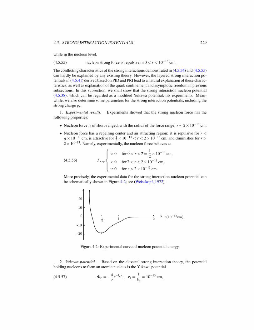
4.5. STRONG INTERACTION POTENTIALS 229
while in the nucleon level,
(4.5.55) nucleon strong force is repulsive in 0 < r < 10−13 cm.
The conflicting characteristics of the strong interactions demonstrated in (4.5.54) and (4.5.55)
can hardly be explained by any existing theory. However, the layered strong interaction po-
tentials in (4.5.41) derived based on PID and PRI lead to a natural explanation of these charac-
teristics, as well as explanation of the quark confinement and asymptotic freedom in previous
subsections. In this subsection, we shall show that the strong interaction nucleon potential
(4.5.38), which can be regarded as a modified Yukawa potential, fits experiments. Mean-
while, we also determine some parameters for the strong interaction potentials, including the
strong charge gs.
1. Experimental results. Experiments showed that the strong nucleon force has the
following properties:
• Nucleon force is of short-ranged, with the radius of the force range: r ∼ 2×10⁻¹³ cm.
• Nucleon force has a repelling center and an attracting region: it is repulsive for r <12× 10−13 cm, is attractive for 1
2× 10⁻¹³ < r < 2× 10⁻¹³ cm, and diminishes for r >
2× 10⁻¹³. Namely, experimentally, the nucleon force behaves as
(4.5.56) Fexp
> 0 for 0 < r < r =1
2× 10⁻¹³ cm,
< 0 for r < r < 2× 10⁻¹³ cm,
⋍ 0 for r > 2× 10⁻¹³ cm.
More precisely, the experimental data for the strong interaction nucleon potential can
be schematically shown in Figure 4.2; see (Weisskopf, 1972).
0
10
20
-10
-20
11
22
r(10−13cm)
Figure 4.2: Experimental curve of nucleon potential energy.
2. Yukawa potential. Based on the classical strong interaction theory, the potential
holding nucleons to form an atomic nucleus is the Yukawa potential
(4.5.57) ΦY =−g
re−knr, r1 =
1
kn
= 10−13 cm,
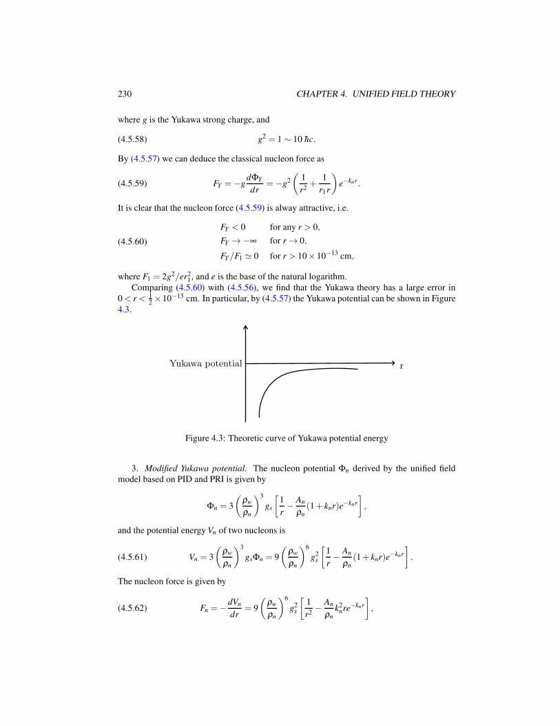
230 CHAPTER 4. UNIFIED FIELD THEORY
where g is the Yukawa strong charge, and
(4.5.58) g2 = 1 ∼ 10 hc.
By (4.5.57) we can deduce the classical nucleon force as
(4.5.59) FY =−gdΦY
dr=−g2
(1
r2+
1
r1r
)e−knr.
It is clear that the nucleon force (4.5.59) is alway attractive, i.e.
(4.5.60)
FY < 0 for any r > 0,
FY →−∞ for r → 0,
FY/F1 ≃ 0 for r > 10× 10−13 cm,
where F1 = 2g2/er21, and e is the base of the natural logarithm.
Comparing (4.5.60) with (4.5.56), we find that the Yukawa theory has a large error in
0 < r < 12×10−13 cm. In particular, by (4.5.57) the Yukawa potential can be shown in Figure
4.3.
Yukawa potential r
Figure 4.3: Theoretic curve of Yukawa potential energy
3. Modified Yukawa potential. The nucleon potential Φn derived by the unified field
model based on PID and PRI is given by
Φn = 3
(ρw
ρn
)3
gs
[1
r− An
ρn
(1+ knr)e−knr
],
and the potential energy Vn of two nucleons is
(4.5.61) Vn = 3
(ρw
ρn
)3
gsΦn = 9
(ρw
ρn
)6
g2s
[1
r− An
ρn
(1+ knr)e−knr
].
The nucleon force is given by
(4.5.62) Fn =−dVn
dr= 9
(ρw
ρn
)6
g2s
[1
r2− An
ρn
k2nre−knr
],
4.5. STRONG INTERACTION POTENTIALS 231
where
(4.5.63) ρn = 10−16 cm, kn = 1013 cm−1.
4. Parameters An and g2s . First, we use the experimental data in (4.5.56) to determine the
parameter An in (4.5.62). By (4.5.56) we know that
Fexp = 0 at r =1
2× 10⁻¹³ cm.
Hence, let
Fn = 0 at r =1
2× 10⁻¹³ cm.
Then, it follows from (4.5.62) and (4.5.63) that
(4.5.64) An = ρneknr/k2nr3 = 8e1/2 × 10−3.
Next, we assume that
(4.5.65) Fn = FY at r1 = 10−13 cm.
Then, by (4.5.59) and (4.5.62), we deduce from (4.5.65) that
9
(ρw
ρn
)6
g2s
[1
r21
− An
ρn
k2nr1e−1
]=−g2 2
r21
e−1,
which leads to
g2s =
2
9
ρn
(Anknr21 − eρn)
(ρn
ρw
)6
g2.
In view of (4.5.63)-(4.5.64) and r1 = 1/kn, we derive
(4.5.66) g2s =
2
9
e−1/2
8− e1/2
(ρn
ρw
)6
g2,
where e = 2.718 and g is as in (4.5.58).
Finally, from Fn = 0 we can also deduce that
Fn > 0 as r > r2 ⋍ 9× 10⁻¹³ cm.
4.5.6 Physical conclusions for nucleon force
The discussion above leads to the following physical conclusions:
1. The modified Yukawa potential based on PID and PRI is
(4.5.67) Φn = β g
[1
r− 8e1/2
r1
(1+r
r1
)e−r/r1
],
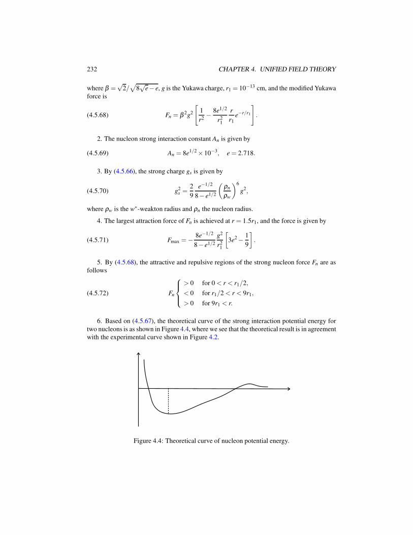
232 CHAPTER 4. UNIFIED FIELD THEORY
where β =√
2/√
8√
e− e, g is the Yukawa charge, r1 = 10−13 cm, and the modified Yukawa
force is
(4.5.68) Fn = β 2g2
[1
r2− 8e1/2
r21
r
r1
e−r/r1
].
2. The nucleon strong interaction constant An is given by
(4.5.69) An = 8e1/2 × 10−3, e = 2.718.
3. By (4.5.66), the strong charge gs is given by
(4.5.70) g2s =
2
9
e−1/2
8− e1/2
(ρn
ρw
)6
g2,
where ρw is the w∗-weakton radius and ρn the nucleon radius.
4. The largest attraction force of Fn is achieved at r = 1.5r1, and the force is given by
(4.5.71) Fmax =− 8e−1/2
8− e1/2
g2
r21
[3e2 − 1
9
].
5. By (4.5.68), the attractive and repulsive regions of the strong nucleon force Fn are as
follows
(4.5.72) Fn
> 0 for 0 < r < r1/2,
< 0 for r1/2 < r < 9r1,
> 0 for 9r1 < r.
6. Based on (4.5.67), the theoretical curve of the strong interaction potential energy for
two nucleons is as shown in Figure 4.4, where we see that the theoretical result is in agreement
with the experimental curve shown in Figure 4.2.
Figure 4.4: Theoretical curve of nucleon potential energy.
4.5. STRONG INTERACTION POTENTIALS 233
4.5.7 Short-range nature of strong interaction
By the layered potentials (4.5.41) for the strong interaction, we see that when the nucleons
form an atom, the nucleon potential is no longer valid, and the correct potential becomes
the strong interaction potential for atoms given by the fourth formula in (4.5.41). The corre-
sponding force formula is given by
(4.5.73) Fa = N2
(ρw
ρa
)6
g2s
[1
r2− Aa
ρa
k2are−kar
],
where
(4.5.74)for atom : ka = 10−9 ∼ 10−10 cm, ρa = 10−8 cm,
for molecule: ka = 10−7 cm, ρa = 10−7 cm.
It is clear that the attractive force in (4.5.73) is of short-ranged. The repulsive force in
(4.5.73) looks as if it is long-ranged. However by (4.5.74) the factors (ρw/ρa)6 for the atoms
and molecules are very small. Hence, the strong repulsive forces for atoms and molecules
almost vanishes.
In fact, the bound force between atoms and molecules is the electromagnetic force with
strength given by
(4.5.75)e2
hc=
1
137, e the electric charge.
Hence at the atomic and molecular scale, the ratio between strong repulsive force and the
electromagnetic force is
(4.5.76)Fa
Fe
= N2s g2
s
(ρw
ρa
)6
/N2e e2,
where Ns is the number of strong charge, and Ne is the number of the electric charge. Note
that each nucleon has three strong charges, and the protons are almost the same as neutrons.
Therefore, we assume that
Ns = 6Ne.
In view of (4.5.70), the ratio (4.5.76) becomes
Fa
Fe
= 4β 2
(ρn
ρa
)6
g2/e2, β 2 =2
8√
e− e⋍ 0.2.
By (4.5.58) and (4.5.75), we have
g2
e2is in the range of
1
137∼ 1
13.7.
Then, by ρn = 10−16 cm and (4.5.74), we derive that
Fa
Fe
∼
10−50 at the atom level,10−56 at the molecular level.
This clearly demonstrates the short-range nature of the strong interaction.
234 CHAPTER 4. UNIFIED FIELD THEORY
4.6 Weak Interaction Theory
4.6.1 Dual equations of weak interaction potentials
According to the standard model, weak interaction is described by the SU(2) gauge theory.
In Section 4.3.4, we have demonstrated that the weak interaction potential is given by the
following PRI representation invariant
(4.6.1) Wµ = ωaW aµ = (W0,W1,W2,W3),
where ωa | 1 ≤ a ≤ 3 is the SU(2) tensor as in (4.3.29).
Also, the weak charge potential and weak force are as
(4.6.2)Φw =W0 the time component of Wµ ,
Fw =−gw(ρ)∇Φw,
where gw(ρ) is the weak charge of a particle with radius ρ .
In this subsection, we establish the field equations for the dual potential Φw and φw of the
weak interaction from the field equations (4.4.48)-(4.4.50).
Taking inner products of (4.4.48) and (4.4.49) with ωa respectively, we derive the field
equations of the two dual weak interaction potentials Φw and φw as follows
∂ νWνµ − gw
hcκabgαβW a
αµW bβ − gwJw
µ = (∂µ − 1
4k2xµ +
gw
hcγWµ)φw,(4.6.3)
[1
c2
∂ 2
∂ t2−∆
]φw + k2
0φw − gw∂ µ Jwµ(4.6.4)
=gw
hc∂ µ[κabgαβW a
αµW bβ − γWµφw
]− 1
4k2
0xµ∂ µφw,
where κab = εcabωc, Wµ is as in (4.6.1), φw = ωaφa
w, and
(4.6.5) Jwµ = ωaψγµσaψ , Wµν = ∂µWν − ∂νWµ +
gw
hcκabW a
µW bν .
Experiments showed that the SU(2) gauge fields W aµ for weak interaction field particles
possess masses. In addition, the dual Higgs fields φaw of W a
µ also have masses. In (4.6.3),
there is no massive term of Wµ . However, we see that on the right-hand side of (4.6.3) there
is a term
(4.6.6)gw
hcγφwWµ ,
which is spontaneously generated by PID, and breaks the gauge-symmetry. Namely, (4.6.6)
will vary under the following SU(2) gauge transformation
W aµ →W a
µ − εabcθ bW c
µ −1
gw
∂µθ a
We shall show that it is the spontaneous symmetry breaking term (4.6.6) that generates mass
from the ground state of φw.
4.6. WEAK INTERACTION THEORY 235
It is clear that the following state
(W aµ ,φ
aw,ψ) = (0,φa
0 ,0) with φa0 being constants,
is a solution of (4.6.3) and (4.6.4), which is a ground state of φaw. Let a0 = φa
0 ωa, which is a
constant. Take the transformation
φw → φw + a0, W aµ →W a
µ , ψ → ψ .
Then the equations (4.6.3) and (4.6.4) are rewritten as
∂ νWνµ − k21Wµ − gw
hcκabgαβW a
αµW bβ − gwJw
µ(4.6.7)
=
[∂µ − 1
4k2
0xµ +gw
hcγWµ
]φµ − 1
4a0k2
0xµ ,
[ 1
c2
∂
∂ t2−∆]φw + k2
0φw − gw∂ µ Jwµ + k2
0a0(4.6.8)
=gw
hc∂ µ[κabgαβW a
αµW bβ − γWµ(φµ + a0)
]− 1
4k2
0xµ∂ µ φw,
where k1 =√
gwγa0/hc represents mass.
Thus, (4.6.7) and (4.6.8) have masses as
(4.6.9) k0 = mHc/h, k1 = mW c/h,
where mH and mW are the masses of Higgs and W± bosons. Physical experiments measured
the values of mH and mW as
(4.6.10) mH ⋍ 160 GeV/c2, mW ⋍ 80 GeV/c2.
By (4.4.46), equations (4.6.7) and (4.6.8) need to add three gauge fixing equations. Based
on the superposition property of the weak charge forces, the dual potentials W0 and φw should
satisfy linear equations, i.e. the time-component µ = 0 equation of (4.6.7) and the equation
(4.6.8) should be linear. Therefore, we have to take the three gauge fixing equations in the
following forms
(4.6.11)
κab
[gαβW a
α0W bβ − ∂ µ(W a
µW b0 )]+ γW0φw − hc
gw
a0k20
4x0 = 0,
gw
hc∂ µ[κabgαβW a
αµW bβ − γWµφw
]− k2
0
4xµ∂ µ φw − k2
0a0 = 0,
∂ µWµ = 0,
and with the static conditions
(4.6.12)∂
∂ tΦw = 0,
∂
∂ tφw = 0, (Φw =W0).
With the equations (4.6.11) and the static conditions (4.6.12), the time-component µ = 0
equation of (4.6.7) and its dual equation (4.6.8) become
−∆Φw + k21Φw = gwQw − 1
4k2
0cτφw,(4.6.13)
−∆φw + k20φw = gw∂ µ Jw
µ ,(4.6.14)
236 CHAPTER 4. UNIFIED FIELD THEORY
where cτ is the wave length of φw,Qw =−Jw0 , and Jw
µ is as in (4.6.5). The two dual equations
(4.6.13) and (4.6.14) for the weak interaction potentials Φw and φw are coupled with the Dirac
equations (4.4.50), written as
(4.6.15) iγµ(
∂µ + igw
hcW a
µ σa
)ψ − mc
hψ = 0.
In addition, by (4.6.9) and (4.6.10) we can determine values of the parameters k0 and k1 as
follows
(4.6.16) k0 = 2k1, k1 = 1016 cm−1.
The parameters 1/k0 and 1/k1 represent the attracting and repulsive radii of weak interaction
forces.
In the next subsection, we shall apply the equations (4.6.13)-(4.6.15) to derive the layered
formulas of weak interaction potentials.
4.6.2 Layered formulas of weak forces
Now we deduce from (4.6.13)-(4.6.16) the following layered formulas for the weak interac-
tion potential:
(4.6.17)
Φw = gw(ρ)e−kr
[1
r− B
ρ(1+ 2kr)e−kr
],
gw(ρ) = N
(ρw
ρ
)3
gw,
where Φw is the weak force potential of a particle with radius ρ and carrying N weak charges
gw (gw is the unit of weak charge for each weakton, an elementary particle), ρw is the weakton
radius, B is a parameter depending on the particles, and
(4.6.18)1
k= 10−16 cm,
represents the force-range of weak interaction.
To derive the layered formulas (4.6.17), first we shall deduce the following weak interac-
tion potential for a weakton
(4.6.19) Φ0w = gse
−kr
[1
r− B0
ρw
(1+ 2kr)e−kr
].
To derive the solution φw of (4.6.14), we need to compute the right-hand term of (4.6.14).
By (4.6.5) we have
∂ µ Jwµ = ωa∂µψγµσa +ωaψγµσa∂µ ψ .
Due to the dirac equation (4.6.15),
∂µψγµσaψ =−igw
hcW b
µ ψγµσbσaψ + imc
hψσaψ ,
ψγµσa∂µψ = igw
hcW b
µ ψγµσaσbψ − imc
hψσaψ .
4.6. WEAK INTERACTION THEORY 237
Thus we obtain
∂ µ Jwµ = i
gw
hcωaW b
µ ψγµ [σa,σb]ψ =−2gw
hcεc
abωaW bµ Jµ
c .(4.6.20)
Here we used [σa,σb] = i2εcabσc and J
µc = ψγµσcψ . Note that
εcabωaW b
µ =
∣∣∣∣∣∣
~i ~j ~kω1 ω2 ω3
W 1µ W 2
µ W 3µ
∣∣∣∣∣∣= ~ω × ~Wµ ,
where ~ω = (ω1,ω2,ω3), ~Wµ = (W 1µ ,W
2µ ,W
3µ ). Hence, (4.6.20) can be rewritten as
(4.6.21) ∂ µJwµ =−2gw
hc(~ω × ~Wµ) · ~Jµ ,
and ~Jµ = (Jµ1 ,J
µ2 ,J
µ3 ). The weak current density J
µa is as
Jµa = θ µ
a δ (r), θ µa the constant tensor,
and ~Wµ in (4.6.21) is replaced by the average value
(4.6.22)1
|Bρw |
∫
Bρw
~Wµdx,
where Bρw ⊂ Rn is the ball with radius ρw. Similar to the case (4.5.14) for the strong interac-
tion, the average value (4.6.22) is
~Wµ = ~ζµ/ρw, ~ζµ = (ζ 1µ ,ζ
2µ ,ζ
3µ).
Thus, (4.6.21) can be expressed as
(4.6.23) ∂ µ Jwµ =−κδ (r)/ρw,
and κ is a parameter, written as
(4.6.24) κ =2gw
hc~θ µ · (~ω ×~ζµ).
Putting (4.6.23) in (4.6.14) we deduce that
−∆φw + k20φw =−gwκ
ρw
δ (r),
whose solution is given by
(4.6.25) φw =−gwκ
ρw
1
re−k0r.
Therefore we obtain the solution of (4.6.14) in the form (4.6.25).
238 CHAPTER 4. UNIFIED FIELD THEORY
Inserting (4.6.25) into (4.6.13) we get
(4.6.26) −∆Φw + k21Φw = gwQw +
gwB
ρw
1
re−k0r,
where B is a parameter with dimension 1/L, given by
B =1
4κk2
0cτ, κ is as in (4.6.24).
Since gwQw =−gwJw0 is the weak charge density, we have
Qw = β δ (r),
and β is a scaling factor. We can take proper unit for gs such that β = 1. Thus, putting
Qw = δ (r) in (4.6.26) we derive that
(4.6.27) −∆Φw + k21Φw = gwδ (r)+
gwB
ρw
1
re−k0r.
Let the solution of (4.6.27) be radially symmetric, then the equation (4.6.27) can be equiva-
lently written as
(4.6.28) − 1
r2
d
dr
(r2 d
dr
)Φw + k2
1Φw = gwδ (r)+gwB
ρw
1
re−k0r.
The solution of (4.6.28) can be expressed as
(4.6.29) Φw =gw
re−k1r − gwB
ρw
ϕ(r)e−k0r,
where ϕ(r) satisfies the equation
(4.6.30) ϕ ′′+ 2
(1
r− k0
)ϕ ′−
(2k0
r+ k2
1 − k20
)ϕ =
1
r.
Let ϕ be in the form
ϕ =∞
∑n=0
βnrn ( the dimension of ϕ is L).
Inserting ϕ into (4.6.30), comparing coefficients of rn, we get
β1 = k0β0 +1
2,
β2 =1
2(k2
0 − k21)β0 +
1
3k0,
...
βn =2k0
n+ 1βn−1 − (k2
0 − k21)βn−2, n ≥ 2.
4.6. WEAK INTERACTION THEORY 239
Note that the dimensions of B and β0 in ϕ(r) are 1/L and L. The parameter B = Bβ0 is
dimensionless. Physically, we can only measure the value of B. Therefore we take ϕ in its
second-order approximation as follows
ϕ = β0(1+ k0r).
In addition, by (4.6.16) we take
k1 = k, k0 = 2k, k = 1016 cm−1.
Thus, the formula (4.6.29) is written as
Φs = gwe−kr
[1
r− B
ρw
(1+ 2kr)e−kr
].
This is the weak interaction potential of a weakton, which is as given in (4.6.19).
In the same fashion as used in the layered formula (4.5.39) for the strong interaction, for
a particle with radius ρ and N weak charges gw, we can deduce the layered formula of weak
interaction potentials as in the form given by (4.6.17).
4.6.3 Physical conclusions for weak forces
As mentioned earlier, the layered weak interaction potential formula (4.6.17) plays the same
fundamental role as the Newtonian potential for gravity and the Coulomb potential for elec-
tromagnetism. Hereafter we explore a few direct physical consequences of the weak interac-
tion potentials.
1. Short-range nature of weak interaction. By (4.6.17) it is easy to see that for all
particles, their weak interaction force-range is as
r =1
k= 10−16 cm,
which is consistent with experimental data.
2. Weak force formula. For two particles with radii ρ1,ρ2, and with N1,N2 weak charges
gw. Their weak charges are given by
(4.6.31) gw(ρ j) = N j
(ρw
ρ j
)3
gw for j = 1,2.
The weak potential energy for the two particles is
(4.6.32) V = gw(ρ1)gw(ρ2)e−kr
[1
r− B
ρ(1+ 2kr)e−kr
],
where gw(ρ1) and gw(ρ2) are as in (4.6.31), ρ is a radius depending on ρ1 and ρ2, and B is a
constant depending on the types of these two particles.
240 CHAPTER 4. UNIFIED FIELD THEORY
The weak force between the two particles is given by
(4.6.33) F =− d
drV = gw(ρ1)gw(ρ2)e
−kr
[1
r2+
k
r− 4B
ρk2re−kr
].
3. Repulsive condition. For the two particles as above, if their weak interaction constant
B satisfies the inequality
1
r2+
k
r≥ 4B
ρk2re−kr, ∀0 < r ≤ 1
k,
or equivalently B satisfies
(4.6.34) B ≤ e
2ρk (e = 2.718, k = 1016 cm−1),
then the weak force between these two particles is always repulsive.
It follows from this conclusion that for the neutrinos:
(ν1,ν2,ν3) = (νe,νµ ,ντ ),
(ν1,ν2,ν3) = (νe,ν µ ,ντ ),
the weak interaction constants
Bi j for νi and ν j ∀1 ≤ i, j ≤ 3,
Bi j for νi and anti-neutrinos ν j ∀i 6= j,
satisfy the exclusion condition (4.6.34).
4. Value of weak charge gw. Based on the Standard Model, the coupling constant Gw of
the β -decay of nucleons and the Fermi constant G f have the following relation
(4.6.35) G2w =
8√2
(mW c
h
)2
G f ,
and G f is given by
(4.6.36) G f = 10−5hc/(mpc
h
)2
,
where mW and mp are masses of W± bosons and protons. By the gauge theory, Gw is also the
coupling constant of SU(2) gauge fields. Therefore we can regard Gw as the weak charge of
nucleons, i.e.
Gw = gw(ρn), ρn the nucleon radius.
In addition, it is known that
gw(ρn) = 9
(ρw
ρn
)3
gs.
4.6. WEAK INTERACTION THEORY 241
Hence, we deduce from (4.6.35) and (4.6.36) that
81
(ρw
ρn
)6
g2w =
8√2
(mw
mp
)2
× 10−5hc.
Then we derive the relation
(4.6.37) g2w =
8
81√
2
(mw
mp
)2
× 10−5 ×(
ρn
ρw
)6
hc.
In a comparison with (4.5.66) and (4.6.37), we find that the strong charge gs and the weak
charge gw have the same magnitude order. Direct computation shows that
g2w
g2s
≃ 0.35 equivalentlygw
gs
≃ 0.6.
4.6.4 PID mechanism of spontaneous symmetry breaking
In the derivation of equations (4.6.7) and (4.6.8) we have used the PID mechanism of sponta-
neous symmetry breaking. In this subsection we shall discuss the intermediate vector bosons
W±,Z and their dual scalar bosons H±,H0, called the Higgs particles by using the PID mech-
anism of spontaneous symmetry breaking.
We know that the interaction field equations are oriented toward two directions: i) to
derive interaction forces, and ii) to describe the field particles and derive the particle transition
probability. The PID-PRI weak interaction field equations describing field particles are given
by (4.4.42)-(4.4.45). Here, for convenience, we write them again as follows:
∂ νW aνµ − gw
hcεa
bcgαβW bαµW c
β − gwJaµ = (∂µ − 1
4
(mHc
h
)2
xµ +gw
hcγbW b
µ )φa,(4.6.38)
− ∂ µ∂µ φa +(mHc
h
)2
φa − gw
hcγb∂ µ(W b
µ φa)(4.6.39)
=gw
hcεa
bcgαβ ∂ µ(W bαµW c
β )+ gw∂ µ Jaµ −
1
4(
mHc
h)2xµ∂ µφa,
where mH is the Higgs particle mass, and W aµ (1 ≤ a ≤ 3) describe the intermediate vector
bosons as follows
(4.6.40)W± : W 1
µ ± iW2µ ,
Z : W 3µ ,
and φa describe the dual Higgs bosons as
(4.6.41)H± : φ1 ± iφ2,
H0 : φ3.
By (4.4.46), equations (4.6.38)-(4.6.39) need to be supplemented with three gauge fixing
equations. According to physical requirement, we take these equations as
(4.6.42) ∂ µW aµ = 0 for 1 ≤ a ≤ 3.
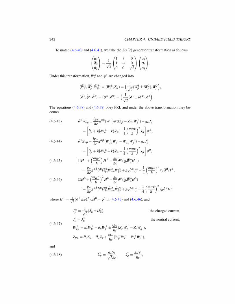
242 CHAPTER 4. UNIFIED FIELD THEORY
To match (4.6.40) and (4.6.41), we take the SU(2) generator transformation as follows
σ1
σ2
σ3
=
1√2
1 i 0
1 −i 0
0 0√
2
σ1
σ2
σ3
.
Under this transformation, W aµ and φa are changed into
(W 1µ ,W
2µ ,W
3µ ) = (W±
µ ,Zµ) =( 1√
2(W 1
µ ± iW2µ ),W
3µ
),
(φ1, φ2, φ3) = (φ±,φ0) =( 1√
2(φ1 ± iφ2),φ3
).
The equations (4.6.38) and (4.6.39) obey PRI, and under the above transformation they be-
comes
∂ νW±νµ ±
igw
hcgαβ (W±)αµZβ −ZαµW±
β )− gwJ±µ(4.6.43)
=
[∂µ + k2
WW±µ + k2
ZZµ − 1
4
(mHc
h
)2
xµ
]φ±,
∂ ν Zνµ − igw
hcgαβ (W+
αµW−β −W−
αµW+β )− gwJ0
µ(4.6.44)
=
[∂µ + k2
WW±µ + k2
ZZµ − 1
4
(mHc
h
)2
xµ
]φ0,
H±+(mHc
h
)H±− gw
hc∂ µ(γbW b
µ H±)(4.6.45)
=gw
hcgαβ ∂ µ(ε±bcW
bαµW c
β )+ gw∂ µ J±µ − 1
4
(mHc
h
)2
xµ∂ µ H±,
H0 +(mHc
h
)2
H0 − gw
hc∂ µ(γbW b
µ H0)(4.6.46)
=gw
hcgαβ ∂ µ(ε0
bcWbαµW c
β )+ gw∂ µ J0µ −
1
4
(mHc
h
)2
xµ∂ µH0,
where H± = 1√2(φ1 ± iφ2),H0 = φ3 in (4.6.45) and (4.6.46), and
(4.6.47)
J±µ =1√2(J1
µ ± iJ2µ) the charged current,
J0µ = J3
µ the neutral current,
W±νµ = ∂νW±
µ − ∂µW±ν ± igw
hc(ZµW±
ν −ZνW±µ ),
Zνµ = ∂νZµ − ∂µZν +igw
hc(W+
µ W−ν −W+
ν W−µ ),
and
(4.6.48) k2W =
gwγ1√2hc
, k2Z =
gwγ3
hc,
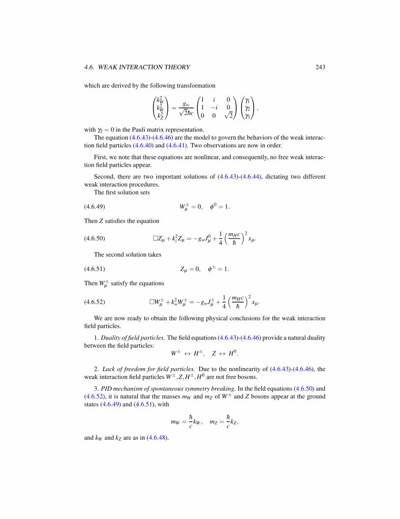
4.6. WEAK INTERACTION THEORY 243
which are derived by the following transformation
k2W
k2W
k2Z
=
gw√2hc
1 i 0
1 −i 0
0 0√
2
γ1
γ2
γ3
,
with γ2 = 0 in the Pauli matrix representation.
The equation (4.6.43)-(4.6.46) are the model to govern the behaviors of the weak interac-
tion field particles (4.6.40) and (4.6.41). Two observations are now in order.
First, we note that these equations are nonlinear, and consequently, no free weak interac-
tion field particles appear.
Second, there are two important solutions of (4.6.43)-(4.6.44), dictating two different
weak interaction procedures.
The first solution sets
(4.6.49) W±µ = 0, φ0 = 1.
Then Z satisfies the equation
(4.6.50) Zµ + k2z Zµ =−gwJ0
µ +1
4
(mHc
h
)2
xµ .
The second solution takes
(4.6.51) Zµ = 0, φ± = 1.
Then W±µ satisfy the equations
(4.6.52) W±µ + k2
wW±µ =−gwJ±µ +
1
4
(mHc
h
)2
xµ .
We are now ready to obtain the following physical conclusions for the weak interaction
field particles.
1. Duality of field particles. The field equations (4.6.43)-(4.6.46) provide a natural duality
between the field particles:
W± ↔ H±, Z ↔ H0.
2. Lack of freedom for field particles. Due to the nonlinearity of (4.6.43)-(4.6.46), the
weak interaction field particles W±,Z,H±,H0 are not free bosons.
3. PID mechanism of spontaneous symmetry breaking. In the field equations (4.6.50) and
(4.6.52), it is natural that the masses mW and mZ of W± and Z bosons appear at the ground
states (4.6.49) and (4.6.51), with
mW =h
ckW , mZ =
h
ckZ,
and kW and kZ are as in (4.6.48).
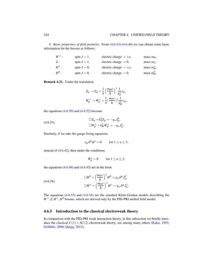
244 CHAPTER 4. UNIFIED FIELD THEORY
4. Basic properties of field particles. From (4.6.43)-(4.6.46) we can obtain some basic
information for the bosons as follows:
W± : spin J = 1, electric charge =±e, mass mW ,
Z : spin J = 1, electric charge = 0, mass mZ ,
H± : spin J = 0, electric charge =±e, mass m+H ,
H0 : spin J = 0, electric charge = 0, mass m0H .
Remark 4.21. Under the translation
Zµ → Zµ +1
4
(mHc
h
)2 1
k2Z
xµ ,
W±µ →W±
µ +1
4(
mHc
h)2 1
k2W
xµ ,
the equations (4.6.50) and (4.6.52) become
(4.6.53)Zµ + k2
ZZµ =−gwJ0µ ,
W±µ + k2
WW±µ =−gwJ±µ .
Similarly, if we take the gauge fixing equations
xµ∂ µ φa = 0 for 1 ≤ a ≤ 3,
instead of (4.6.42), then under the conditions
W aµ = 0 for 1 ≤ a ≤ 3,
the equations (4.6.46) and (4.6.45) are in the form
(4.6.54)
H0 +(mHc
h
)2
H0 = gw∂ µJ0µ ,
H±+(mHc
h
)2
H± = gw∂ µ J±µ .
The equations (4.6.53) and (4.6.54) are the standard Klein-Gordon models describing the
W±,Z,H±,H0 bosons, which are derived only by the PID-PRI unified field model.
4.6.5 Introduction to the classical electroweak theory
In comparison with the PID-PRI weak interaction theory, in this subsection we briefly intro-
duce the classical U(1)× SU(2) electroweak theory; see among many others (Kaku, 1993;
Griffiths, 2008; Quigg, 2013).
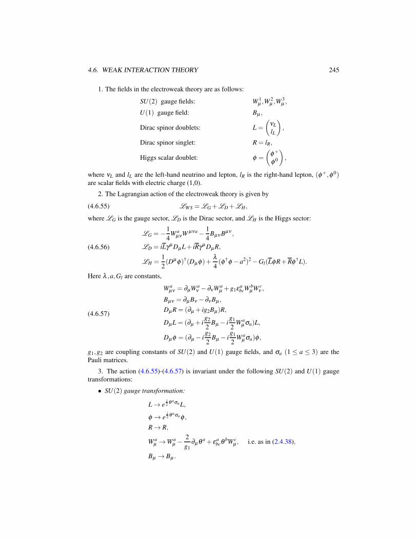
4.6. WEAK INTERACTION THEORY 245
1. The fields in the electroweak theory are as follows:
SU(2) gauge fields: W 1µ ,W
2µ ,W
3µ ,
U(1) gauge field: Bµ ,
Dirac spinor doublets: L =
(νL
lL
),
Dirac spinor singlet: R = lR,
Higgs scalar doublet: φ =
(φ+
φ0
),
where νL and lL are the left-hand neutrino and lepton, lR is the right-hand lepton, (φ+,φ0)are scalar fields with electric charge (1,0).
2. The Lagrangian action of the electroweak theory is given by
(4.6.55) LWS = LG +LD +LH,
where LG is the gauge sector, LD is the Dirac sector, and LH is the Higgs sector:
(4.6.56)
LG =−1
4W a
µνW µνa − 1
4BµνBµν ,
LD = iLγµ DµL+ iRγµ DµR,
LH =1
2(Dµφ)†(Dµφ)+
λ
4(φ†φ − a2)2 −Gl(LφR+Rφ†L).
Here λ ,a,Gl are constants,
(4.6.57)
W aµν = ∂µW a
ν − ∂νW aµ + g1εa
bcWbµW c
ν ,
Bµν = ∂µ Bν − ∂νBµ ,
DµR = (∂µ + ig2Bµ)R,
DµL = (∂µ + ig2
2Bµ − i
g1
2W a
µ σa)L,
Dµφ = (∂µ − ig2
2Bµ − i
g1
2W a
µ σa)φ ,
g1,g2 are coupling constants of SU(2) and U(1) gauge fields, and σa (1 ≤ a ≤ 3) are the
Pauli matrices.
3. The action (4.6.55)-(4.6.57) is invariant under the following SU(2) and U(1) gauge
transformations:
• SU(2) gauge transformation:
L → ei2 θ aσa L,
φ → ei2 θ aσa φ ,
R → R,
W aµ →W a
µ − 2
g1
∂µθ a + εabcθ bW c
µ , i.e. as in (2.4.38),
Bµ → Bµ .
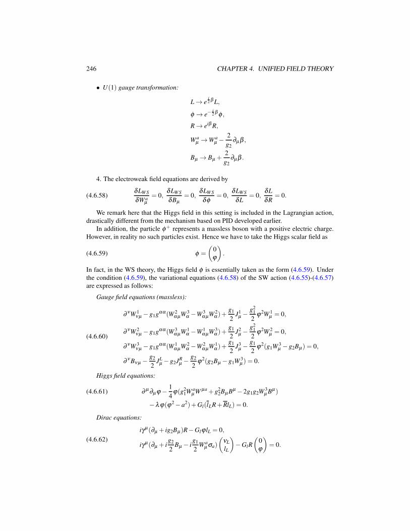
246 CHAPTER 4. UNIFIED FIELD THEORY
• U(1) gauge transformation:
L → ei2 β L,
φ → e−i2 β φ ,
R → eiβ R,
W aµ →W a
µ − 2
g2
∂µβ ,
Bµ → Bµ +2
g2
∂µβ .
4. The electroweak field equations are derived by
(4.6.58)δLW S
δW aµ
= 0,δLW S
δBµ= 0,
δLW S
δφ= 0,
δLW S
δL= 0,
δL
δR= 0.
We remark here that the Higgs field in this setting is included in the Lagrangian action,
drastically different from the mechanism based on PID developed earlier.
In addition, the particle φ+ represents a massless boson with a positive electric charge.
However, in reality no such particles exist. Hence we have to take the Higgs scalar field as
(4.6.59) φ =
(0
ϕ
).
In fact, in the WS theory, the Higgs field φ is essentially taken as the form (4.6.59). Under
the condition (4.6.59), the variational equations (4.6.58) of the SW action (4.6.55)-(4.6.57)
are expressed as follows:
Gauge field equations (massless):
(4.6.60)
∂ νW 1νµ − g1gαα(W 2
αµW 3α −W3
αµW 2α )+
g1
2J1
µ −g2
1
2ϕ2W 1
µ = 0,
∂ νW 2νµ − g1gαα(W 3
αµW 1α −W1
αµW 3α )+
g1
2J2
µ −g2
1
2ϕ2W 2
µ = 0,
∂ νW 3νµ − g1gαα(W 1
αµW 2α −W2
αµW 1α )+
g1
2J3
µ −g1
2ϕ2(g1W 3
µ − g2Bµ) = 0,
∂ νBνµ − g2
2JL
µ − g2JRµ − g2
2ϕ2(g2Bµ − g1W 3
µ ) = 0.
Higgs field equations:
∂ µ ∂µϕ − 1
4ϕ(g2
1W aµW µa + g2
2BµBµ − 2g1g2W 3µ Bµ)(4.6.61)
−λ ϕ(ϕ2 − a2)+Gl(lLR+RlL) = 0.
Dirac equations:
(4.6.62)
iγµ(∂µ + ig2Bµ)R−Glϕ lL = 0,
iγµ(∂µ + ig2
2Bµ − i
g1
2W a
µ σa)
(νL
lL
)−GlR
(0
ϕ
)= 0.
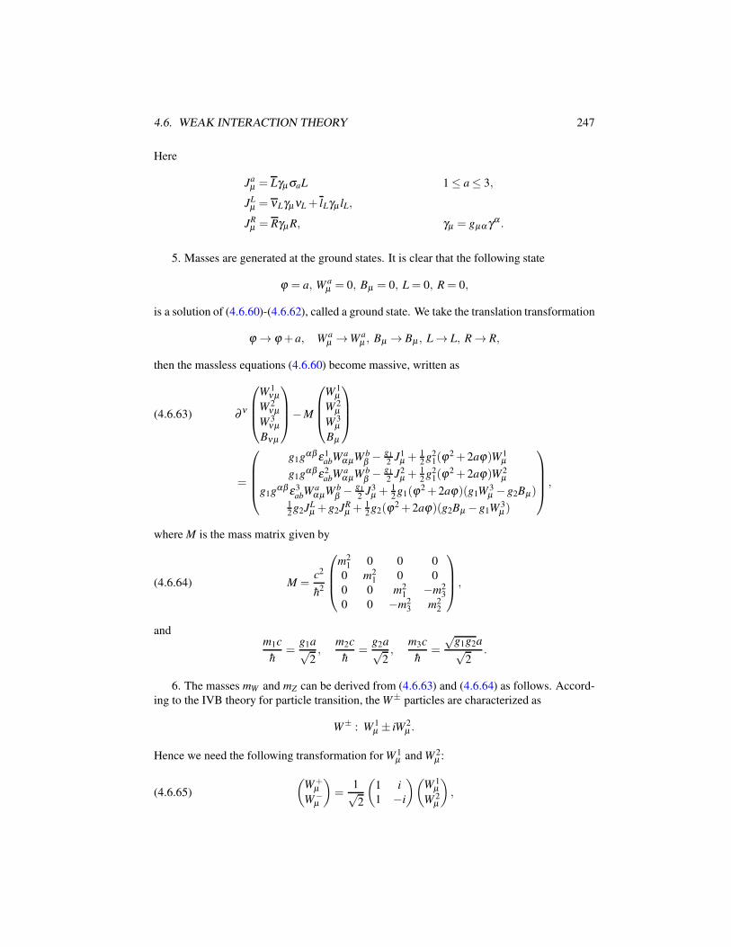
4.6. WEAK INTERACTION THEORY 247
Here
Jaµ = LγµσaL 1 ≤ a ≤ 3,
JLµ = νLγµνL + lLγµ lL,
JRµ = Rγµ R, γµ = gµα γα .
5. Masses are generated at the ground states. It is clear that the following state
ϕ = a, W aµ = 0, Bµ = 0, L = 0, R = 0,
is a solution of (4.6.60)-(4.6.62), called a ground state. We take the translation transformation
ϕ → ϕ + a, W aµ →W a
µ , Bµ → Bµ , L → L, R → R,
then the massless equations (4.6.60) become massive, written as
∂ ν
W 1νµ
W 2νµ
W 3νµ
Bνµ
−M
W 1µ
W 2µ
W 3µ
Bµ
(4.6.63)
=
g1gαβ ε1abW a
αµW bβ − g1
2J1
µ +12g2
1(ϕ2 + 2aϕ)W1
µ
g1gαβ ε2abW a
αµW bβ − g1
2J2
µ +12g2
1(ϕ2 + 2aϕ)W2
µ
g1gαβ ε3abW a
αµW bβ − g1
2J3
µ + 12g1(ϕ
2 + 2aϕ)(g1W3µ − g2Bµ)
12g2JL
µ + g2JRµ + 1
2g2(ϕ
2 + 2aϕ)(g2Bµ − g1W 3µ )
,
where M is the mass matrix given by
(4.6.64) M =c2
h2
m21 0 0 0
0 m21 0 0
0 0 m21 −m2
3
0 0 −m23 m2
2
,
andm1c
h=
g1a√2,
m2c
h=
g2a√2,
m3c
h=
√g1g2a√
2.
6. The masses mW and mZ can be derived from (4.6.63) and (4.6.64) as follows. Accord-
ing to the IVB theory for particle transition, the W± particles are characterized as
W± : W 1µ ± iW2
µ .
Hence we need the following transformation for W 1µ and W 2
µ :
(4.6.65)
(W+
µ
W−µ
)=
1√2
(1 i
1 −i
)(W 1
µ
W 2µ
),
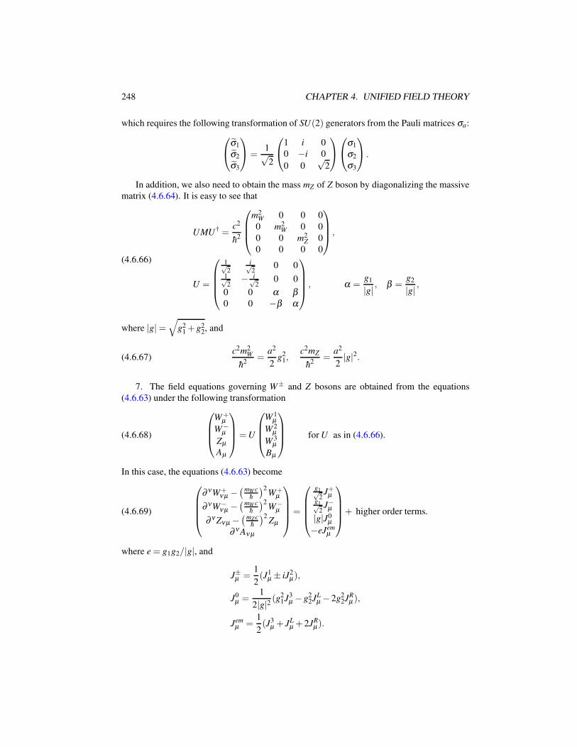
248 CHAPTER 4. UNIFIED FIELD THEORY
which requires the following transformation of SU(2) generators from the Pauli matrices σa:
σ1
σ2
σ3
=
1√2
1 i 0
0 −i 0
0 0√
2
σ1
σ2
σ3
.
In addition, we also need to obtain the mass mZ of Z boson by diagonalizing the massive
matrix (4.6.64). It is easy to see that
(4.6.66)
UMU† =c2
h2
m2W 0 0 0
0 m2W 0 0
0 0 m2Z 0
0 0 0 0
,
U =
1√2
i√2
0 01√2
− i√2
0 0
0 0 α β0 0 −β α
, α =
g1
|g| , β =g2
|g| ,
where |g|=√
g21 + g2
2, and
(4.6.67)c2m2
W
h2=
a2
2g2
1,c2mZ
h2=
a2
2|g|2.
7. The field equations governing W± and Z bosons are obtained from the equations
(4.6.63) under the following transformation
(4.6.68)
W+µ
W−µ
Zµ
Aµ
=U
W 1µ
W 2µ
W 3µ
Bµ
for U as in (4.6.66).
In this case, the equations (4.6.63) become
(4.6.69)
∂ νW+νµ −
(mW c
h
)2W+
µ
∂ νW−νµ −
(mW c
h
)2W−
µ
∂ ν Zνµ −(
mZ ch
)2Zµ
∂ ν Aνµ
=
g1√2J+µ
g1√2J−µ
|g|J0µ
−eJemµ
+ higher order terms.
where e = g1g2/|g|, and
J±µ =1
2(J1
µ ± iJ2µ),
J0µ =
1
2|g|2 (g21J3
µ − g22JL
µ − 2g22JR
µ ),
Jemµ =
1
2(J3
µ + JLµ + 2JR
µ).
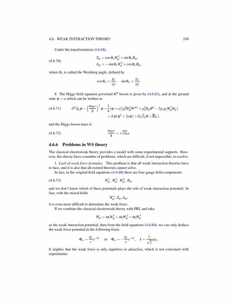
4.6. WEAK INTERACTION THEORY 249
Under the transformation (4.6.68),
(4.6.70)Zµ = cosθwW 3
µ + sinθwBµ ,
Aµ =−sinθwW 3µ + cosθwBµ ,
where θw is called the Weinberg angle, defined by
cosθw =g1
|g| , sinθw =g2
|g| .
8. The Higgs field equation governed H0 boson is given by (4.6.61), and at the ground
state ϕ = a which can be written as
∂ µ∂µϕ −(mHc
h
)2
ϕ =1
4(ϕ + a)(g2
1WaµW µa + g2
2BµBµ − 2g1g2W 3µ Bµ)(4.6.71)
+λ ϕ(ϕ2 + 2aϕ)+Gl(lLR+RlL),
and the Higgs boson mass is
(4.6.72)mHc
h=√
2λa.
4.6.6 Problems in WS theory
The classical electroweak theory provides a model with some experimental supports. How-
ever, this theory faces a number of problems, which are difficult, if not impossible, to resolve.
1. Lack of weak force formulas. This problem is that all weak interaction theories have
to face, and it is also that all existed theories cannot solve.
In fact, in the original field equations (4.6.60) there are four gauge field components:
(4.6.73) W 1µ , W 2
µ , W 3µ , Bµ ,
and we don’t know which of these potentials plays the role of weak interaction potential. In
fact, with the mixed fields
W±µ ,Zµ ,Aµ ,
it is even more difficult to determine the weak force.
If we combine the classical electroweak theory with PRI, and take
Wµ = ω1W 1µ +ω2W 2
µ +ω3W3µ
as the weak interaction potential, then from the field equations (4.6.60), we can only deduce
the weak force potential in the following form:
Φw =g1
re−kr or Φw =−g1
re−kr, k =
1√2
ag1.
It implies that the weak force is only repulsive or attractive, which is not consistent with
experiments.
250 CHAPTER 4. UNIFIED FIELD THEORY
2. Violation of PRI. In the classical electroweak theory, a key ingredient is the linear
combinations of W 3µ and Bµ as given by (4.6.70). By PRI,
W 3µ is the third component of a SU(2) tensor Wa
µ,Bµ is the U(1) gauge field.
Hence, for the combinations of two different types of tensors:
Zµ = cosθwW 3µ + sinθwBµ ,
Aµ =−sinθwW 3µ + cosθwBµ ,
their field equations (4.6.69) must vary under general SU(2) generator transformations as
follows
(4.6.74) σa = xbaσb.
In other words, such linear combinations violates PRI.
3. Decoupling obstacle. The classical electroweak theory has a difficulty for decoupling
the electromagnetic and the weak interactions. In reality, electromagnetism and weak interac-
tion often are independent to each other. Hence, as a unified theory for both interactions, one
should be able to decouple the model to study individual interactions. However, the classical
electroweak theory manifests a radical decoupling obstacle.
In fact, it is natural to require that under the condition
(4.6.75) W±µ = 0, Zµ = 0,
the WS field equations (4.6.69) should return to the U(1) gauge invariant Maxwell equations.
But we see that
Aµ = cosθwBµ − sinθwW 3µ ,
where Bµ is a U(1) gauge field, and W 3µ is a component of SU(2) gauge field. Therefore, Aµ is
not independent of SU(2) gauge transformation. In particular, the condition (4.6.75) means
(4.6.76) W 1µ = 0, W 2
µ = 0, W 3µ =− tgθwBµ .
Hence, as we take the transformation (4.6.74), W aµ becomes
W 1µ
W 2µ
W 3µ
=
y13W 3
µ
y23W 3
µ
y33W 3
µ
, (yb
a)T = (xb
a)−1.
It implies that under a transformation (4.6.74), a nonzero weak interaction can be generated
from a zero weak interaction field of (4.6.75)-(4.6.76):
W±µ 6= 0, Zµ 6= 0 as ya
3 6= 0 (1 ≤ a ≤ 3),
and the nonzero electromagnetic field Aµ 6= 0 will become zero:
Aµ = 0 as y33 = cotθw.
4.6. WEAK INTERACTION THEORY 251
Obviously, it is not reality.
4. Artificial Higgs mechanism. In the classical electroweak action (4.6.55)-(4.6.57), the
Higgs sector LH is not based on a first principle, and is artificially added into the action.
5. Presence of a massless and charged boson φ+. In the WS theory, the Higgs scalar
doublet φ = (φ+φ0) contains a massless boson φ+ with positive electric charge. Obviously
there are no such particles in reality. In particular, the particle φ+ is ”formally suppressed” in
the WS theory by transforming it to zero in the WS theory. However, from a field theoretical
point of view, this particle field still represents a particle. This is one of major flaws for the
electroweak theory and for the standard model.

252 CHAPTER 4. UNIFIED FIELD THEORY
Chapter 5
Elementary Particles
The aims of this chapter are as follows:
1) to give a brief introduction to the particle physics,
2) to introduce the weakton model of elementary particles,
3) to address the mechanism of subatomic decays,
4) to introduce color algebra, as the mathematical basis for the color quantum number,
and
5) to derive the structure of mediator clouds around subatomic particles.
Searching for the main constituents of matter has a long history going back to ancient
Greeks, to Robert Boyle (1600s), John Dalton (early 1800s), J.J. Thomson and Ernest Ruther-
ford (end of the 19th century), and Niels Bohr (1913).
In the current standard model of particle physics, all forms of matter are made up of 6
leptons and 6 quarks, and their antiparticles, which are treated as elementary particles. The
forces are mediated by the mediators, including the photon mediating the electromagnetism,
the vector bosons W±, Z and the Higgs H0 mediating the weak interaction, the eight gluons
mediating the strong interaction, and the hypothetical graviton mediating gravity.
However, there are many challenging problems related to subatomic particles. One such
problem is that why leptons do not participate in strong interactions. In fact, the most difficult
challenge is associated with the puzzling decay and reaction behavior of subatomic particles.
For example, the electron radiations and the electron-positron annihilation into photons or
quark-antiquark pair clearly shows that there must be interior structure of electrons, and the
constituents of an electron contribute to the making of photon or the quark in the hadrons
formed in the process. In fact, all sub-atomic decays and reactions show clearly the following
conclusion:
There must be interior structure of charged leptons, quarks and mediators.
253
254 CHAPTER 5. ELEMENTARY PARTICLES
This conclusion motivates us to propose a weakton model for sub-lepton, sub-quark, and
sub-mediators (Ma and Wang, 2015b), based on the new field theory and the new insights for
the weak and strong interactions presented in the last chapter.
One important theoretical basic for the weakton model is the field theory developed in
the last chapter. In particular, the weak and strong charges are responsible for the weak
and strong interactions. The confinement property demonstrated by the weak and strong
interaction potentials give rise to the needed confinement for the weakton constituents of the
composite particles.
Remarkably, the weakton model offers a perfect explanation for all sub-atomic decays. In
particular, all decays are achieved by 1) exchanging weaktons and consequently exchanging
newly formed quarks, producing new composite particles, and 2) separating the new compos-
ite particles by weak and/or strong forces.
One aspect of this decay mechanism is that now we know the precise constituents of
particles involved in all decays/reactions both before and after the reaction. It is therefore
believed that the new decay mechanism provides clear new insights for both experimental
and theoretical studies.
This chapter is organized as follows. Sections 5.1 and 5.2 recall the basic knowledge of
particle physics and the quark model. Sections 5.3 and 5.4 are based entirely on (Ma and Wang,
2015b), with the weakton model introduced in Section 5.3, and with the mechanism of sub-
atomic decays and electron radiations presented in Section 5.4. The last section, Section 5.5
studies the color algebra associated with the color quantum number, leading to detailed
structure on mediator clouds around subatomic particles. Section 5.5 is based entirely on
(Ma and Wang, 2014b).
5.1 Basic Knowledge of Particle Physics
5.1.1 Classification of particles
In particle physics, subatomic particles are classified into two basic classes, bosons and
fermions:bosons = integral spin particles,
fermions = fractional spin particles.
Also, based on their properties and levels, all subatomic particles are currently classified into
four types:
leptons, quarks, mediators, hadrons.
In the following, we recall basic definitions and the quantum characterizations of these parti-
cles; see among many others (Kane, 1987; Griffiths, 2008; Halzen and Martin, 1984).
1. Leptons. Leptons are fermions which do not participate in the strong interaction, and
consist of three generations:
(e
νe
),
(µ ,νµ
),
(τντ
),
5.1. BASIC KNOWLEDGE OF PARTICLE PHYSICS 255
where e,µ ,τ are the electron, the muon, the tau, and νe,νµ ,ντ are the e-neutrino, the µ-
neutrino, the τ-neutrino. Together with their antiparticles, there are total 12 leptons:
particles: (e−,νe), (µ−,νµ), (τ−,ντ ),
antiparticles: (e+,νe), (µ+,νµ), (τ+,ντ).
2. Quarks. Based on the standard model, there are three generations of quarks consisting
of 6 particles and 6 antiparticles, which participate all four fundamental interactions:
quarks: (u,d), (c,s), (t,b),
antiquarks: (u,d), (c,s), (t,b),
where u,d,c,s, t,b are the up quark, down quark, charm quark, strange quark, top quark, and
bottom quark.
The quark model asserts that three quarks are bounded together to form a baryon, and a
pair of quark and antiquark are bounded to form a meson. As mentioned in Section 4.5.3,
quarks are confined in hadrons, and no free quarks have been found in Nature. This phe-
nomena is called the quark confinement, which has been very well explained by the layered
formulas of strong interactions in the last chapter.
3. Mediators. The standard model shows that each interaction is associated with a class
of field particles, called mediators. Hence, there are four classes of mediators:
Gravitation: graviton G,
Electromagnetism: photon γ,
Weak interaction: vector and Higgs bosons W±,Z,H±,H0,
Strong interaction: gluons gk (1 ≤ k ≤ 8).
By the unified field theory introduced in the last chapter, there exists a natural duality
between the interacting fields gµν ,Aµ ,Waµ ,S
kµ and their dual fields φg
µ ,φe,φa
w,φks :
gµν ↔ φgµ ,
Aµ ↔ φ e,
W aµ ↔ φa
w, 1 ≤ a ≤ 3,
Skµ ↔ φ k
s , 1 ≤ k ≤ 8.
This duality leads to four classes of new dual particle fields, called the dual mediators:
(5.1.1)
tensor graviton G ↔ vector graviton g,
vector photon γ ↔ scalar photon γ0,
charged vector bosons W± ↔ charged Higgs bosons H±,
neutral vector boson Z ↔ neutral Higgs boson H0,
vector gluons gk ↔ scalar gluons gk0, 1 ≤ k ≤ 8,
256 CHAPTER 5. ELEMENTARY PARTICLES
where the upper index k in gk and gk0 represents the color index of gluons.
The mediator duality (5.1.1) is derived from the unified field theory. However, the duality
(5.1.1) can also be naturally deduced from the weakton model postulated in Section 5.3.
Namely, the mediator duality (5.1.1) is derived from two very different perspectives in two
different theories. This can hardly be a coincident.
4. Hadrons. Hadrons are classified into two types: baryons and mesons. Baryons are
fermions and mesons are bosons, which are all made up of quarks:
Baryons = qiq jqk, mesons = qiq j,
where qk = u,d,c,s, t,b. The quark constituents of main hadrons are listed as follows:
• Baryons with J = 12:
p (uud), n (udd), Λ (s(du− ud)/√
2),
Σ+ (uus), Σ− (dds), Σ0 (s(du+ ud)/√
2),
Ξ0 (uss), Ξ− (dss).
• Baryons with J = 32:
∆++ (uuu), ∆+ (uud), ∆− (ddd), ∆0 (udd),
Σ∗+(uus), Σ∗−(dds), Σ0(uds),
Ξ∗0(uss), Ξ∗−(dss), Ω−(sss).
• Mesons with J = 0:
π+(ud), π−(ud), π0((uu− dd)/√
2),
K+(us), K−(us), K0(ds),
K0(ds), η((uu+ dd− 2ss)/
√6).
• Mesons with J = 1:
ρ+(ud), ρ−(ud), ρ0((uu− dd)/√
2),
K∗+(us), K∗−(us), K∗0(ds),
K∗0(ds), ψ(cc), γ(bb).
5.1.2 Quantum numbers
It is easy to identify a macro-body, but not easy to identify a sub-atomic particle. Usually
experimental physicists distinguish these sub-atomic particles by measuring their physical
parameters. There are numerous types of particles, which obey various conservation laws.
Each conservation law is characterized by one parameter. These physical parameters are
called quantum numbers.
5.1. BASIC KNOWLEDGE OF PARTICLE PHYSICS 257
The main quantum numbers of particles are:
(5.1.2)
mass m, electric charge Q, lifetime τ,
spin J, lepton number L, baryon number B,
parity π , isospin (I, I3), strange number S,
G-parity, hypercharge Y.
In addition, there are some new quantum numbers, including the weak charge Qw, strong
charge Qs, and colour index k, which play an important role in in the weakton model intro-
duced in Section 5.3.
We now briefly introduce the quantum numbers listed in (5.1.2).
1 Mass. This is a quantity to characterize the inertia, and also plays the role of gravita-
tional charge. In the macro-world, masses are continuous in distribution, however in quantum
world masses are discrete. The same particles have the same masses, but the different massive
particles have a gap between their masses.
In non-quantum physics, the masses are additive, i.e. if a body A consists of two bodies
B and C, then the mass mA of A is the sum of masses mB and mC of B and C:
(5.1.3) A = B+C ⇒ mA = mB +mC.
But, the additive relation (5.1.3) is not valid in a quantum system.
Mass is a most important quantum number, which plays a role of an identity card for all
massive particles.
2. Electric charge Q. This is an important quantum number. It is the source of electro-
magnetic force. In the four interaction charges: m,e,gw,gs, the electric charge e is unique
one possessing positive and negative values. The electric charges are discrete, they appear
only at an integral multiples of the electron charge e: 1
Q =±ne (n = 0,1,2, · · ·).
Electric charge is an additive conservation quantity. For any particle reaction:
A1 + · · ·+An → B1 + · · ·BN ,
we haven
∑k=1
QAk=
N
∑k=1
QBk,
where QAkand QBk
are the electric charges of particles Ak and Bk
3. Lifetime of particles. Due to the decay property for most particles, the lifetime becomes
a quantum number. Except the long lifetime particles: the electron e, proton p, neutrino v,
photon γ , gluon gk, graviton G, all other particles undergo decays.
1In the weakton model of elementary particles, w∗ carries 2/3 electric charge, and w1 and w2 carry −1/3 and
−2/3 electric charges respectively.
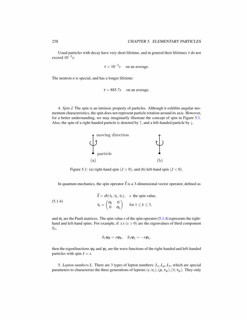
258 CHAPTER 5. ELEMENTARY PARTICLES
Usual particles with decay have very short lifetime, and in general their lifetimes τ do not
exceed 10−5s:
τ < 10−5s on an average.
The neutron n is special, and has a longer lifetime:
τ = 885.7s on an average.
4. Spin J. The spin is an intrinsic property of particles. Although it exhibits angular mo-
mentum characteristics, the spin does not represent particle rotation around its axis. However,
for a better understanding, we may imaginarily illustrate the concept of spin in Figure 5.1.
Also, the spin of a right-handed particle is denoted by ↑, and a left-handed particle by ↓.
(a)
moving direction
particle
(b)
Figure 5.1: (a) right-hand spin (J > 0), and (b) left-hand spin (J < 0).
In quantum mechanics, the spin operator~S is a 3-dimensional vector operator, defined as
(5.1.4)
~S = sh(τ1,τ2,τ3), s the spin value,
τk =
(σk 0
0 σk
)for 1 ≤ k ≤ 3,
and σk are the Pauli matrices. The spin value s of the spin operator (5.1.4) represents the right-
hand and left-hand spins. For example, if ±s (s > 0) are the eigenvalues of third component
S3,
S3ψR = sψR, S3ψL =−sψL,
then the eigenfunctions ψR and ψL are the wave functions of the right-handed and left-handed
particles with spin J = s.
5. Lepton numbers L. There are 3 types of lepton numbers: Le,Lµ ,Lτ , which are special
parameters to characterize the three generations of leptons (e,νe),(µ ,νµ),(τ,νµ ). They only
5.1. BASIC KNOWLEDGE OF PARTICLE PHYSICS 259
take three values L =±1,0. For all non-lepton particles, their lepton number is zero, and
Le =
1 for e−,νe,
− 1 for e+,νe,
0 others,
Lµ =
1 for µ−,νµ ,
− 1 for µ+,νµ ,
0 others,
Lτ =
1 for τ−,ντ ,
− 1 for τ+,ντ ,
0 others.
The lepton numbers are additive and conservative quantities.
6. Baryon number B. The hadrons are classified into baryons and mesons. Baryons are
fermions and mesons are bosons. Also, baryons have an additive and conservative quantum
number: the baryon number B, defined by
B =
1 for a baryon,
− 1 for an antibaryon,
0 for all other particles.
7. Parity π . Due to the Noether Theorem 2.38, each symmetry is associated with a
conservation law. The parity is a conservative quantum number corresponding to the spatial
reflection symmetry:
x →−x (x ∈R3).
Parity π only takes two values:
π =±1.
The weak interaction violates parity; see (Lee and Yang, 1956; Wu, Ambler, Hayward, Hoppes and Hudson,
1957). The parities π of most particles are obtained by two methods: the experimental and
the artificial means.
The parity is a multiplication quantum number. For example, for an N particles system:
A = A1 + · · ·+AN,
its tatol parity πA is given by
πA = (−1)lπA1· · ·πAN
,
where l is the sum of orbital quantum numbers of all particles, and πAkis the parity of Ak
particle.
The parity conservation is defined as follows. For a particle reaction:
(5.1.5) A1 + · · ·+AN −→ B1 + · · ·+BK,
260 CHAPTER 5. ELEMENTARY PARTICLES
the total parities of both sides of (5.1.5) are the same:
(−1)l1πA1· · ·πAN
= (−1)l2πB1· · ·πBK
.
In Subsection 5.1.4, we shall introduce the violation of parity conservation in the weak inter-
action in detail.
8. Isospin (I, I3). The isospin was first presented in 1932 by Heisenberg, and was used to
describe that the strong interaction between protons and neutrons, independently of electric
charges. Later, along with the development of particle physics, it was discovered that the
isospin is a good quantum number for all hadrons.
Isospin has two components (I, I3), where I is called the isospin and I3 is the third com-
ponent of isospin. In a many-particle system, the isospin I obeys the vectorial additive rule
and I3 obeys the usual additive rule. We shall introduce the isospin again in Subsection 5.1.4.
9. Strange number S. In 1947, C. D. Rochester and C. C. Butler first discovered the
strange particle K0, a neutral meson, from cosmic rays, and later many strange particles such
as K±,Λ,Σ±,Ξ−,Ξ0,Ω− were found. They are named the ”strange” because these particles
possess a kind quantum number called the strange number.
The strange number S is an additive quantum number, which is conserved only in the
electromagnetic and strong interactions, and takes the integral values:
S = 0,1,2,3, · · · .
10. Hypercharge Y . Hypercharge Y is another quantum number for hadrons, defined by
Y = S+B,
where S and B are the strange number and the baryon number.
11. G-parity. G parity is a conservative quantity only for strong interactions under the
G-transformation
Gψ = CeiπI2 ψ ,
where C is the transformation of particles and antiparticles:
CA = A, CA = A, A the antiparticle of A,
and I2 is the second axis of the isospin space.
5.1.3 Particle transitions
Particle transition is the main dynamic form of sub-atomic particles, which includes particle
decays, scatterings and various radiations. It is called ”transition” because in these processes
particles will undergo a transition from an energy level to other energy levels.
The particle transition is a crucial way for us to understand the particle structures and
properties. In particular, these transition processes can reveal the mysteries of the weak and
the strong interactions.
5.1. BASIC KNOWLEDGE OF PARTICLE PHYSICS 261
1. Decays. Particle decay means that a particle is spontaneously decomposed into several
other particles. The most remarkable example is the β -decay, i.e., a neutron n decays to a
proton p, an electron e− and an anti-neutrino νe:
(5.1.6) n → p+ e−+νe.
Current list of discovered particle consists of hundreds of numbers. Except electrons
and protons, all massive particles will decay therefore they are finite lifetime. The massless
particles, such as the photon, the gluons and the neutrinos, do not decay, and have infinite
lifetime.
All decays obey the following laws and rules:
1) Decays are caused by the three fundamental forces: the electromagnetic, weak, strong
interactions, and, therefore, are mainly classified into two types: weak interaction de-
cays and strong interaction decays;
2) Decays always take place from higher masses toward to lower masses. For example in
the β -decay (5.1.6), the masses of particles on the right-hand side are smaller than the
mass of the neutron n.
3) Both strong and weak interaction decays have to obey some basic conservation laws,
as shown in the next subsection.
Remark 5.1. The following transition
(5.1.7) p → n+ e++νe
is often called β -decay as well. In fact, in Nature the process (5.1.7) cannot spontaneously
take place, and it always occurs under certain energetic excitation. Hence, (5.1.7) is an excited
scattering.
2. Scattering. If the decay is a spontaneous behavior, then scattering is a forced behavior
of particles under certain force actions, such as collisions and energetic excitations. The
transition (5.1.7) is a scattering, and the precise decay mechanism is written as
p+ γ → n+ e++νe.
In general, a scattering reaction is written as
(5.1.8) A1 + · · ·+AN → B1 + · · ·BK ,
where An (1 ≤ n ≤ N) are the initial particles, and Bk (1 ≤ k ≤ K) are the final particles.
There are two forms of scatterings: the elastic and non-elastic scatterings, both of which
are caused by the three interactions: the electromagnetic, the weak and the strong interac-
tions. Collision is the most important experimental method to detect new particles and new
phenomena. The scatterings (5.1.8) satisfy various conservation relations.
262 CHAPTER 5. ELEMENTARY PARTICLES
Here are a few important scatterings in the history of quantum physics:
Compton scattering: γ + e− → γ + e−,
Pair annihilation: e++ e− → γ + γ,
Pair creation: γ + γ → e++ e−,
Moller scattering: e−+ e− → e−+ e−,
Bhahba scattering: e−+ e+ → e−+ e+.
Deep inelastic scattering : e−+ p → e−+ p+π0.
3. Radiations. Radiations include the electromagnetic radiation and the gluon radiation.
The first one is that electrons emit photons:
(5.1.9) e− → e−+ γ,
and the second one is that quarks emit gluons
(5.1.10) q → q+ gk,
Electromagnetic radiations are caused in two scenaries:
1) As an electron changes its velocity, it emits photons. This radiation is called the
bremsstrahlung. The radiation energy in unit time can be expressed by the formula:
W =2
3
e2
c3a2 with a being the average acceleration.
2) As an electron at a higher energy level E1 undergoes a transition to a lower energy
level E0 < E1, it emits photons. The energy ε of the emitting photons equals to the
difference of energy levels:
ε = E1 −E0.
In summary, there are three types of particle transitions: decays, scatterings, and radia-
tions. They are the main dynamic behavior for micro-particles, and reveal the interior struc-
ture of particles, and provide crucial information about the three interactions associated with
the electromagnetic, the weak, and the strong forces.
Here we list some principal decay forms:
• Lepton decays:
(5.1.11)
µ− → e−+νe +νµ ,
µ+ → e++νe +νµ ,
τ− → e−+νe +ντ ,
τ− → µ−+νµ +ντ ,
τ− → π−+ντ ,
τ− → ρ−+ντ ,
τ− → K−+ντ .
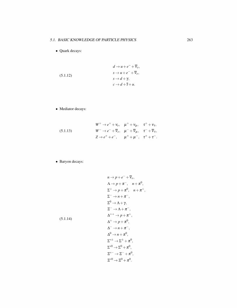
5.1. BASIC KNOWLEDGE OF PARTICLE PHYSICS 263
• Quark decays:
(5.1.12)
d → u+ e−+νe,
s → u+ e−+νe,
s → d+ γ,
c → d + s+ u.
• Mediator decays:
(5.1.13)
W+ → e++νe, µ++νµ , τ++ντ ,
W− → e−+νe, µ−+νµ , τ−+ντ ,
Z → e++ e−, µ++ µ−, τ++ τ−.
• Baryon decays:
(5.1.14)
n → p+ e−+νe,
Λ → p+π−, n+π0,
Σ+ → p+π0, n+π+,
Σ− → n+π−,
Σ0 → Λ+ γ,
Ξ− → Λ+π−,
∆++ → p+π+,
∆+ → p+π0,
∆− → n+π−,
∆0 → n+π0,
Σ∗± → Σ±+π0,
Σ∗0 → Σ0 +π0,
Ξ∗− → Ξ−+π0,
Ξ∗0 → Ξ0 +π0.
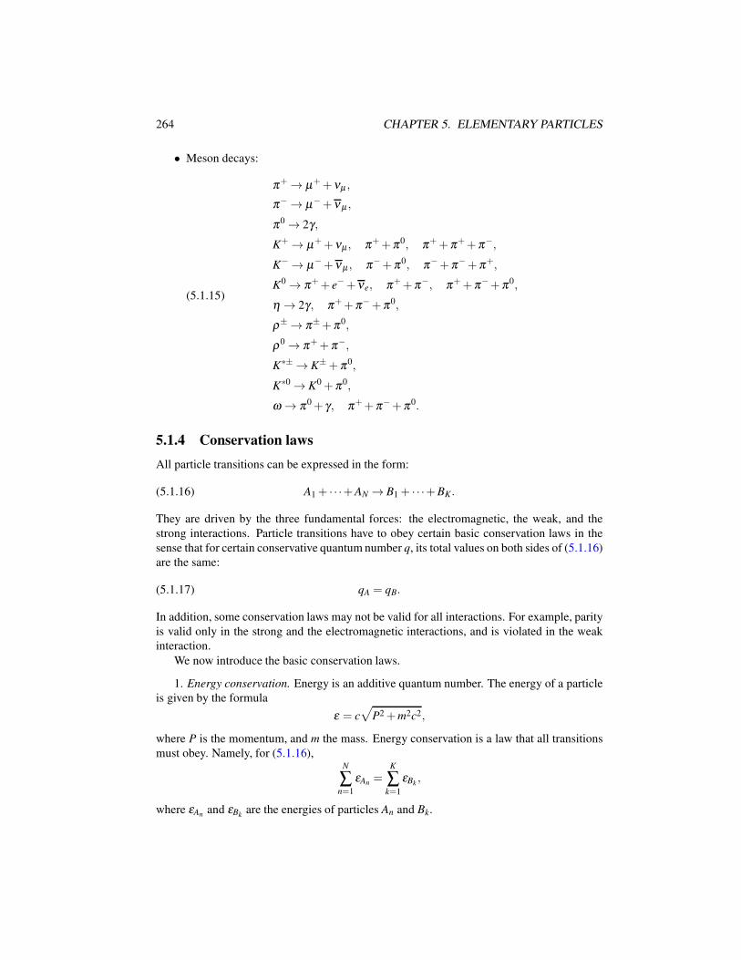
264 CHAPTER 5. ELEMENTARY PARTICLES
• Meson decays:
(5.1.15)
π+ → µ++νµ ,
π− → µ−+νµ ,
π0 → 2γ,
K+ → µ++νµ , π++π0, π++π++π−,
K− → µ−+νµ , π−+π0, π−+π−+π+,
K0 → π++ e−+νe, π++π−, π++π−+π0,
η → 2γ, π++π−+π0,
ρ± → π±+π0,
ρ0 → π++π−,
K∗± → K±+π0,
K∗0 → K0 +π0,
ω → π0 + γ, π++π−+π0.
5.1.4 Conservation laws
All particle transitions can be expressed in the form:
(5.1.16) A1 + · · ·+AN → B1 + · · ·+BK.
They are driven by the three fundamental forces: the electromagnetic, the weak, and the
strong interactions. Particle transitions have to obey certain basic conservation laws in the
sense that for certain conservative quantum number q, its total values on both sides of (5.1.16)
are the same:
(5.1.17) qA = qB.
In addition, some conservation laws may not be valid for all interactions. For example, parity
is valid only in the strong and the electromagnetic interactions, and is violated in the weak
interaction.
We now introduce the basic conservation laws.
1. Energy conservation. Energy is an additive quantum number. The energy of a particle
is given by the formula
ε = c√
P2 +m2c2,
where P is the momentum, and m the mass. Energy conservation is a law that all transitions
must obey. Namely, for (5.1.16),N
∑n=1
εAn =K
∑k=1
εBk,
where εAn and εBkare the energies of particles An and Bk.
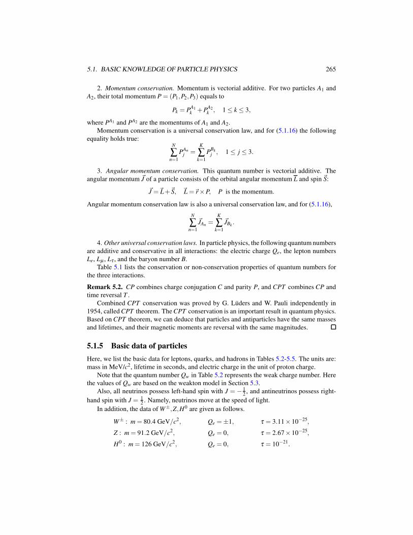
5.1. BASIC KNOWLEDGE OF PARTICLE PHYSICS 265
2. Momentum conservation. Momentum is vectorial additive. For two particles A1 and
A2, their total momentum P = (P1,P2,P3) equals to
Pk = PA1k +P
A2k , 1 ≤ k ≤ 3,
where PA1 and PA2 are the momentums of A1 and A2.
Momentum conservation is a universal conservation law, and for (5.1.16) the following
equality holds true:N
∑n=1
PAnj =
K
∑k=1
PBkj , 1 ≤ j ≤ 3.
3. Angular momentum conservation. This quantum number is vectorial additive. The
angular momentum ~J of a particle consists of the orbital angular momentum L and spin ~S:
~J =~L+~S, ~L =~r×P, P is the momentum.
Angular momentum conservation law is also a universal conservation law, and for (5.1.16),
N
∑n=1
~JAn =K
∑k=1
~JBk.
4. Other universal conservation laws. In particle physics, the following quantum numbers
are additive and conservative in all interactions: the electric charge Qe, the lepton numbers
Le, Lµ , Lτ , and the baryon number B.
Table 5.1 lists the conservation or non-conservation properties of quantum numbers for
the three interactions.
Remark 5.2. CP combines charge conjugation C and parity P, and CPT combines CP and
time reversal T .
Combined CPT conservation was proved by G. Luders and W. Pauli independently in
1954, called CPT theorem. The CPT conservation is an important result in quantum physics.
Based on CPT theorem, we can deduce that particles and antiparticles have the same masses
and lifetimes, and their magnetic moments are reversal with the same magnitudes.
5.1.5 Basic data of particles
Here, we list the basic data for leptons, quarks, and hadrons in Tables 5.2-5.5. The units are:
mass in MeV/c2, lifetime in seconds, and electric charge in the unit of proton charge.
Note that the quantum number Qw in Table 5.2 represents the weak charge number. Here
the values of Qw are based on the weakton model in Section 5.3.
Also, all neutrinos possess left-hand spin with J = − 12, and antineutrinos possess right-
hand spin with J = 12. Namely, neutrinos move at the speed of light.
In addition, the data of W±,Z,H0 are given as follows.
W± : m = 80.4 GeV/c2, Qe =±1, τ = 3.11× 10⁻²⁵,
Z : m = 91.2 GeV/c2, Qe = 0, τ = 2.67× 10⁻²⁵,
H0 : m = 126 GeV/c2, Qe = 0, τ = 10−21.
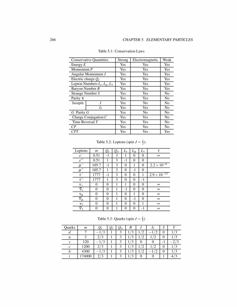
266 CHAPTER 5. ELEMENTARY PARTICLES
Table 5.1: Conservation Laws
Conservative Quantities Strong Electromagnetic Weak
Energy E Yes Yes Yes
Momentum P Yes Yes Yes
Angular Momentum J Yes Yes Yes
Electric charge Qe Yes Yes Yes
Lepton Numbers Le,Lµ ,Lτ Yes Yes Yes
Baryon Number B Yes Yes Yes
Strange Number S Yes Yes No
Parity π Yes Yes No
Isospin I Yes No No
I3 Yes Yes No
G Parity G Yes No No
Charge Conjugation C Yes Yes No
Time Reversal T Yes Yes No
CP Yes Yes No
CPT Yes Yes Yes
Table 5.2: Leptons (spin J = 12).
Leptons m Qe Qw Le Lµ Lτ τe− 0.51 -1 3 1 0 0 ∞
e+ 0.51 1 3 -1 0 0
µ− 105.7 -1 3 0 1 0 2.2× 10⁻⁶
µ+ 105.7 1 3 0 -1 0
τ− 1777 -1 3 0 0 1 2.9× 10⁻¹³
τ+ 1777 1 3 0 0 -1
ν+ 0 0 1 1 0 0 ∞νe 0 0 1 -1 0 0 ∞
νµ 0 0 1 0 1 0 ∞
νµ 0 0 1 0 -1 0 ∞
ντ 0 0 1 0 0 1 ∞
ντ 0 0 1 0 0 -1 ∞
Table 5.3: Quarks (spin J = 12)
Quarks m Qe Qs Qw B I I3 S Y
d 7 −1/3 1 3 1/3 1/2 −1/2 0 1/3
u 3 2/3 1 3 1/3 1/2 1/2 0 1/3
s 120 −1/3 1 3 1/3 0 0 -1 −2/3
c 1200 2/3 1 3 1/3 1/2 1/2 0 1/3
b 4300 −1/3 1 3 1/3 1/2 −1/2 0 1/3
t 174000 2/3 1 3 1/3 0 0 1 4/3
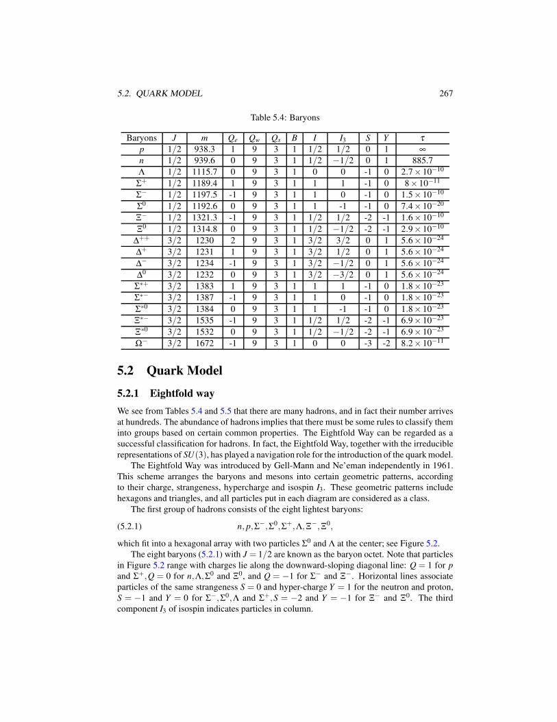
5.2. QUARK MODEL 267
Table 5.4: Baryons
Baryons J m Qe Qw Qs B I I3 S Y τp 1/2 938.3 1 9 3 1 1/2 1/2 0 1 ∞
n 1/2 939.6 0 9 3 1 1/2 −1/2 0 1 885.7
Λ 1/2 1115.7 0 9 3 1 0 0 -1 0 2.7× 10⁻¹⁰
Σ+ 1/2 1189.4 1 9 3 1 1 1 -1 0 8× 10⁻¹¹
Σ− 1/2 1197.5 -1 9 3 1 1 0 -1 0 1.5× 10⁻¹⁰
Σ0 1/2 1192.6 0 9 3 1 1 -1 -1 0 7.4× 10⁻²⁰
Ξ− 1/2 1321.3 -1 9 3 1 1/2 1/2 -2 -1 1.6× 10⁻¹⁰
Ξ0 1/2 1314.8 0 9 3 1 1/2 −1/2 -2 -1 2.9× 10⁻¹⁰
∆++ 3/2 1230 2 9 3 1 3/2 3/2 0 1 5.6× 10⁻²⁴
∆+ 3/2 1231 1 9 3 1 3/2 1/2 0 1 5.6× 10⁻²⁴
∆− 3/2 1234 -1 9 3 1 3/2 −1/2 0 1 5.6× 10⁻²⁴
∆0 3/2 1232 0 9 3 1 3/2 −3/2 0 1 5.6× 10⁻²⁴
Σ∗+ 3/2 1383 1 9 3 1 1 1 -1 0 1.8× 10⁻²³
Σ∗− 3/2 1387 -1 9 3 1 1 0 -1 0 1.8× 10−23
Σ∗0 3/2 1384 0 9 3 1 1 -1 -1 0 1.8× 10⁻²³
Ξ∗− 3/2 1535 -1 9 3 1 1/2 1/2 -2 -1 6.9× 10−23
Ξ∗0 3/2 1532 0 9 3 1 1/2 −1/2 -2 -1 6.9× 10⁻²³
Ω− 3/2 1672 -1 9 3 1 0 0 -3 -2 8.2× 10⁻¹¹
5.2 Quark Model
5.2.1 Eightfold way
We see from Tables 5.4 and 5.5 that there are many hadrons, and in fact their number arrives
at hundreds. The abundance of hadrons implies that there must be some rules to classify them
into groups based on certain common properties. The Eightfold Way can be regarded as a
successful classification for hadrons. In fact, the Eightfold Way, together with the irreducible
representations of SU(3), has played a navigation role for the introduction of the quark model.
The Eightfold Way was introduced by Gell-Mann and Ne’eman independently in 1961.
This scheme arranges the baryons and mesons into certain geometric patterns, according
to their charge, strangeness, hypercharge and isospin I3. These geometric patterns include
hexagons and triangles, and all particles put in each diagram are considered as a class.
The first group of hadrons consists of the eight lightest baryons:
(5.2.1) n, p,Σ−,Σ0,Σ+,Λ,Ξ−,Ξ0,
which fit into a hexagonal array with two particles Σ0 and Λ at the center; see Figure 5.2.
The eight baryons (5.2.1) with J = 1/2 are known as the baryon octet. Note that particles
in Figure 5.2 range with charges lie along the downward-sloping diagonal line: Q = 1 for p
and Σ+,Q = 0 for n,Λ,Σ0 and Ξ0, and Q = −1 for Σ− and Ξ−. Horizontal lines associate
particles of the same strangeness S = 0 and hyper-charge Y = 1 for the neutron and proton,
S = −1 and Y = 0 for Σ−,Σ0,Λ and Σ+,S = −2 and Y = −1 for Ξ− and Ξ0. The third
component I3 of isospin indicates particles in column.
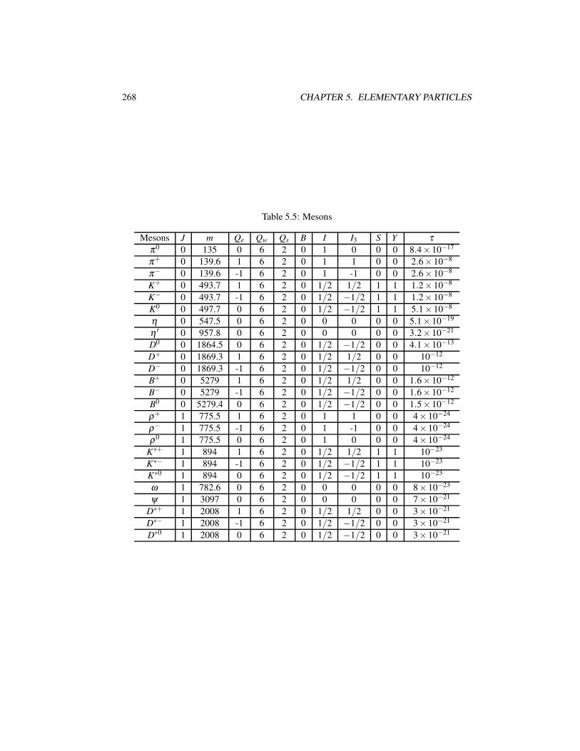
268 CHAPTER 5. ELEMENTARY PARTICLES
Table 5.5: Mesons
Mesons J m Qe Qw Qs B I I3 S Y τ
π0 0 135 0 6 2 0 1 0 0 0 8.4× 10⁻¹⁷
π+ 0 139.6 1 6 2 0 1 1 0 0 2.6× 10⁻⁸
π− 0 139.6 -1 6 2 0 1 -1 0 0 2.6× 10⁻⁸
K+ 0 493.7 1 6 2 0 1/2 1/2 1 1 1.2× 10⁻⁸
K− 0 493.7 -1 6 2 0 1/2 −1/2 1 1 1.2× 10⁻⁸
K0 0 497.7 0 6 2 0 1/2 −1/2 1 1 5.1× 10⁻⁸
η 0 547.5 0 6 2 0 0 0 0 0 5.1× 10⁻¹⁹
η ′ 0 957.8 0 6 2 0 0 0 0 0 3.2× 10⁻²¹
D0 0 1864.5 0 6 2 0 1/2 −1/2 0 0 4.1× 10⁻¹³
D+ 0 1869.3 1 6 2 0 1/2 1/2 0 0 10−12
D− 0 1869.3 -1 6 2 0 1/2 −1/2 0 0 10−12
B+ 0 5279 1 6 2 0 1/2 1/2 0 0 1.6× 10⁻¹²
B− 0 5279 -1 6 2 0 1/2 −1/2 0 0 1.6× 10⁻¹²
B0 0 5279.4 0 6 2 0 1/2 −1/2 0 0 1.5× 10⁻¹²
ρ+ 1 775.5 1 6 2 0 1 1 0 0 4× 10⁻²⁴
ρ− 1 775.5 -1 6 2 0 1 -1 0 0 4× 10⁻²⁴
ρ0 1 775.5 0 6 2 0 1 0 0 0 4× 10⁻²⁴
K∗+ 1 894 1 6 2 0 1/2 1/2 1 1 10−23
K∗− 1 894 -1 6 2 0 1/2 −1/2 1 1 10−23
K∗0 1 894 0 6 2 0 1/2 −1/2 1 1 10−23
ω 1 782.6 0 6 2 0 0 0 0 0 8× 10⁻²³
ψ 1 3097 0 6 2 0 0 0 0 0 7× 10⁻²¹
D∗+ 1 2008 1 6 2 0 1/2 1/2 0 0 3× 10⁻²¹
D∗− 1 2008 -1 6 2 0 1/2 −1/2 0 0 3× 10−21
D∗0 1 2008 0 6 2 0 1/2 −1/2 0 0 3× 10⁻²¹
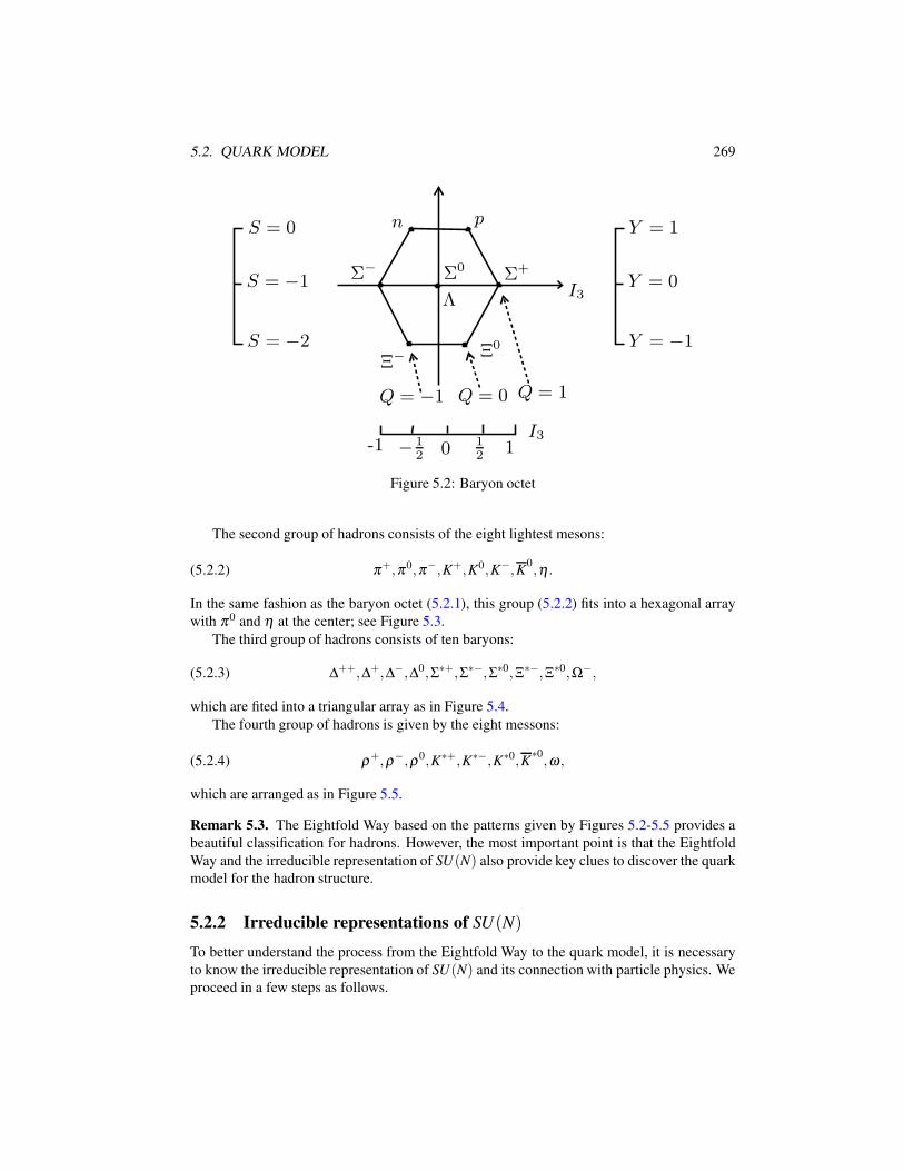
5.2. QUARK MODEL 269
n pS = 0
S = −1
S = −2
Σ− Σ0 Σ+
ΛI3
Ξ− Ξ0
Q = −1 Q = 0 Q = 1
Y = 1
Y = 0
Y = −1
-1 −
1
2 0 1
21
I3
Figure 5.2: Baryon octet
The second group of hadrons consists of the eight lightest mesons:
(5.2.2) π+,π0,π−,K+,K0,K−,K0,η .
In the same fashion as the baryon octet (5.2.1), this group (5.2.2) fits into a hexagonal array
with π0 and η at the center; see Figure 5.3.
The third group of hadrons consists of ten baryons:
(5.2.3) ∆++,∆+,∆−,∆0,Σ∗+,Σ∗−,Σ∗0,Ξ∗−,Ξ∗0,Ω−,
which are fited into a triangular array as in Figure 5.4.
The fourth group of hadrons is given by the eight messons:
(5.2.4) ρ+,ρ−,ρ0,K∗+,K∗−,K∗0,K∗0,ω ,
which are arranged as in Figure 5.5.
Remark 5.3. The Eightfold Way based on the patterns given by Figures 5.2-5.5 provides a
beautiful classification for hadrons. However, the most important point is that the Eightfold
Way and the irreducible representation of SU(N) also provide key clues to discover the quark
model for the hadron structure.
5.2.2 Irreducible representations of SU(N)
To better understand the process from the Eightfold Way to the quark model, it is necessary
to know the irreducible representation of SU(N) and its connection with particle physics. We
proceed in a few steps as follows.
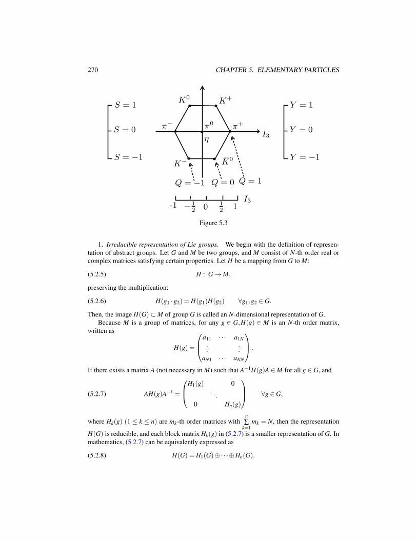
270 CHAPTER 5. ELEMENTARY PARTICLES
K0K+
S = 1
S = 0
S = −1
π− π0π+
ηI3
K− K0
Q = −1 Q = 0 Q = 1
Y = 1
Y = 0
Y = −1
-1 −
1
2 0 1
21
I3
Figure 5.3
1. Irreducible representation of Lie groups. We begin with the definition of represen-
tation of abstract groups. Let G and M be two groups, and M consist of N-th order real or
complex matrices satisfying certain properties. Let H be a mapping from G to M:
(5.2.5) H : G → M,
preserving the multiplication:
(5.2.6) H(g1 ·g2) = H(g1)H(g2) ∀g1,g2 ∈ G.
Then, the image H(G)⊂ M of group G is called an N-dimensional representation of G.
Because M is a group of matrices, for any g ∈ G,H(g) ∈ M is an N-th order matrix,
written as
H(g) =
a11 · · · a1N
......
aN1 · · · aNN
.
If there exists a matrix A (not necessary in M) such that A−1H(g)A ∈ M for all g ∈ G, and
(5.2.7) AH(g)A−1 =
H1(g) 0
. . .
0 Hn(g)
∀g ∈ G,
where Hk(g) (1 ≤ k ≤ n) are mk-th order matrices withn
∑k=1
mk = N, then the representation
H(G) is reducible, and each block matrix Hk(g) in (5.2.7) is a smaller representation of G. In
mathematics, (5.2.7) can be equivalently expressed as
(5.2.8) H(G) = H1(G)⊕·· ·⊕Hn(G).
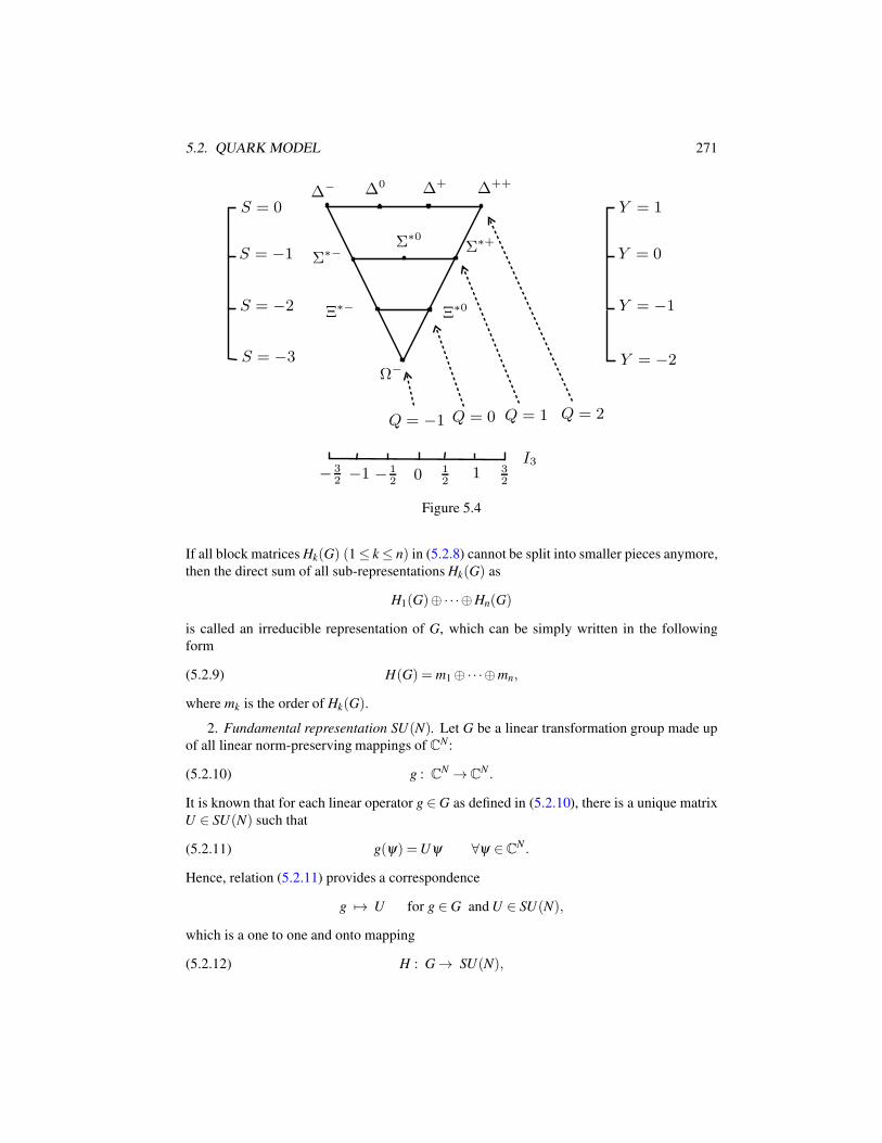
5.2. QUARK MODEL 271
∆− ∆0
S = 0
S = −1
S = −2
Σ∗−
Σ∗0
∆+ ∆++
Σ∗+
Ξ∗0
Q = −1 Q = 0 Q = 1
Y = 1
Y = 0
Y = −1
−1 − 1
20 1
21
I3
S = −3
Ξ∗−
Ω−
Q = 2
Y = −2
−
3
2
3
2
Figure 5.4
If all block matrices Hk(G) (1 ≤ k ≤ n) in (5.2.8) cannot be split into smaller pieces anymore,
then the direct sum of all sub-representations Hk(G) as
H1(G)⊕·· ·⊕Hn(G)
is called an irreducible representation of G, which can be simply written in the following
form
(5.2.9) H(G) = m1 ⊕·· ·⊕mn,
where mk is the order of Hk(G).
2. Fundamental representation SU(N). Let G be a linear transformation group made up
of all linear norm-preserving mappings of CN :
(5.2.10) g : CN →C
N .
It is known that for each linear operator g ∈ G as defined in (5.2.10), there is a unique matrix
U ∈ SU(N) such that
(5.2.11) g(ψ) =Uψ ∀ψ ∈CN .
Hence, relation (5.2.11) provides a correspondence
g 7→ U for g ∈ G and U ∈ SU(N),
which is a one to one and onto mapping
(5.2.12) H : G → SU(N),
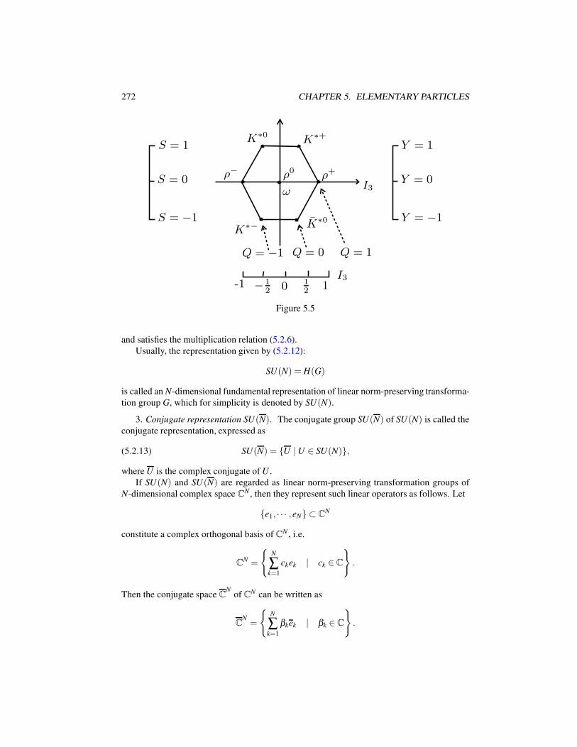
272 CHAPTER 5. ELEMENTARY PARTICLES
K∗0K∗+
S = 1
S = 0
S = −1
ρ−
ρ0ρ+
ωI3
K∗− K∗0
Q = −1 Q = 0 Q = 1
Y = 1
Y = 0
Y = −1
-1 −
1
2 0 1
21
I3
Figure 5.5
and satisfies the multiplication relation (5.2.6).
Usually, the representation given by (5.2.12):
SU(N) = H(G)
is called an N-dimensional fundamental representation of linear norm-preserving transforma-
tion group G, which for simplicity is denoted by SU(N).
3. Conjugate representation SU(N). The conjugate group SU(N) of SU(N) is called the
conjugate representation, expressed as
(5.2.13) SU(N) = U | U ∈ SU(N),
where U is the complex conjugate of U .
If SU(N) and SU(N) are regarded as linear norm-preserving transformation groups of
N-dimensional complex space CN , then they represent such linear operators as follows. Let
e1, · · · ,eN ⊂ CN
constitute a complex orthogonal basis of CN , i.e.
CN =
N
∑k=1
ckek | ck ∈C
.
Then the conjugate space CN
of CN can be written as
CN=
N
∑k=1
βkek | βk ∈ C
.
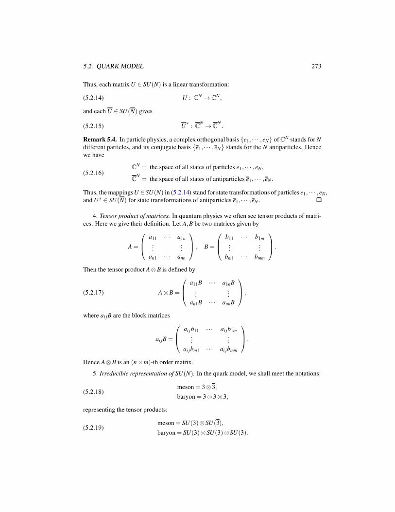
5.2. QUARK MODEL 273
Thus, each matrix U ∈ SU(N) is a linear transformation:
(5.2.14) U : CN →C
N ,
and each U ∈ SU(N) gives
(5.2.15) U∗
: CN → C
N.
Remark 5.4. In particle physics, a complex orthogonal basis e1, · · · ,eN of CN stands for N
different particles, and its conjugate basis e1, · · · ,eN stands for the N antiparticles. Hence
we have
(5.2.16)C
N = the space of all states of particles e1, · · · ,eN ,
CN= the space of all states of antiparticles e1, · · · ,eN .
Thus, the mappingsU ∈ SU(N) in (5.2.14) stand for state transformations of particles e1, · · · ,eN ,
and U∗ ∈ SU(N) for state transformations of antiparticles e1, · · · ,eN .
4. Tensor product of matrices. In quantum physics we often see tensor products of matri-
ces. Here we give their definition. Let A,B be two matrices given by
A =
a11 · · · a1n
......
an1 · · · ann
, B =
b11 · · · b1m
......
bm1 · · · bmm
.
Then the tensor product A⊗B is defined by
(5.2.17) A⊗B =
a11B · · · a1nB...
...
an1B · · · annB
,
where ai jB are the block matrices
ai jB =
ai jb11 · · · ai jb1m
......
ai jbm1 · · · ai jbmm
.
Hence A⊗B is an (n×m)-th order matrix.
5. Irreducible representation of SU(N). In the quark model, we shall meet the notations:
(5.2.18)meson = 3⊗ 3,
baryon = 3⊗ 3⊗ 3,
representing the tensor products:
(5.2.19)meson = SU(3)⊗ SU(3),
baryon = SU(3)⊗ SU(3)⊗ SU(3).
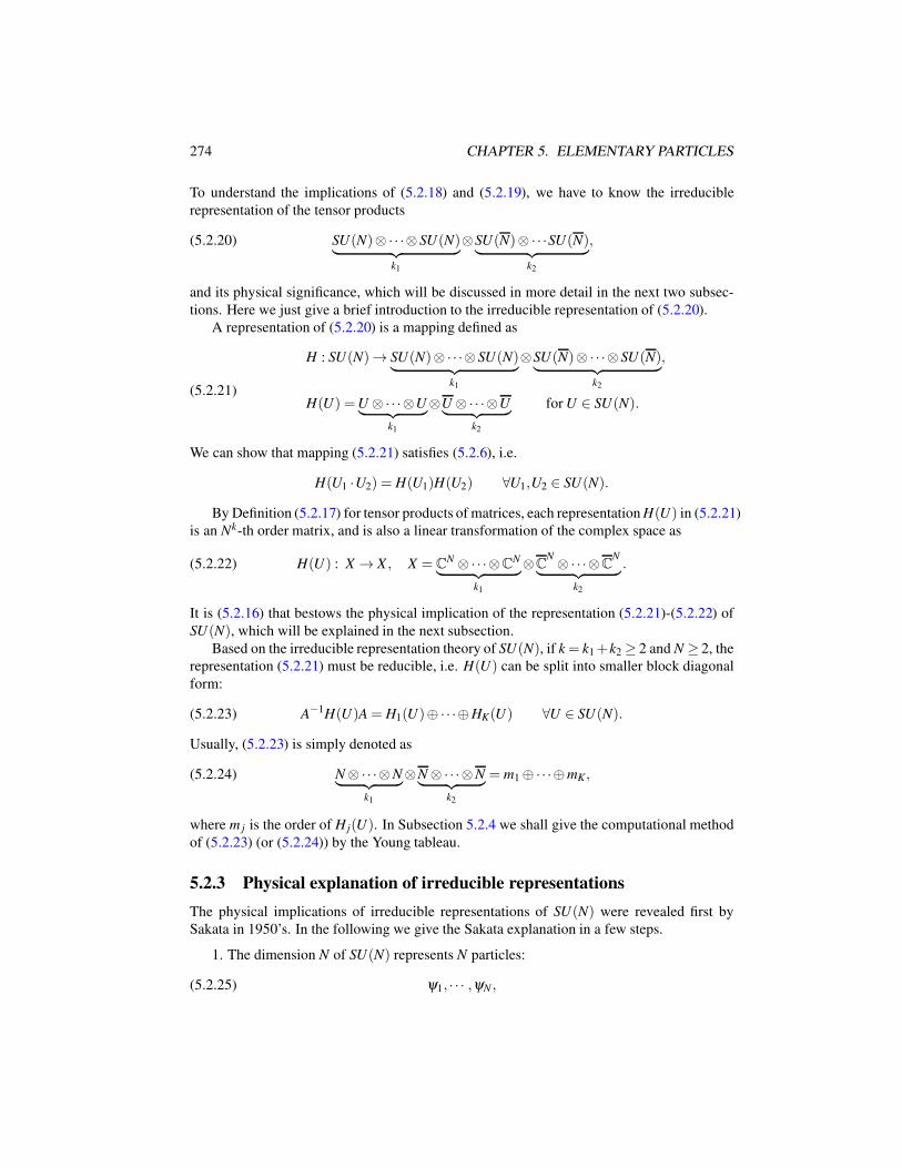
274 CHAPTER 5. ELEMENTARY PARTICLES
To understand the implications of (5.2.18) and (5.2.19), we have to know the irreducible
representation of the tensor products
(5.2.20) SU(N)⊗·· ·⊗ SU(N)︸ ︷︷ ︸k1
⊗SU(N)⊗·· ·SU(N)︸ ︷︷ ︸k2
,
and its physical significance, which will be discussed in more detail in the next two subsec-
tions. Here we just give a brief introduction to the irreducible representation of (5.2.20).
A representation of (5.2.20) is a mapping defined as
(5.2.21)
H : SU(N)→ SU(N)⊗·· ·⊗ SU(N)︸ ︷︷ ︸k1
⊗SU(N)⊗·· ·⊗ SU(N)︸ ︷︷ ︸k2
,
H(U) =U ⊗·· ·⊗U︸ ︷︷ ︸k1
⊗U ⊗·· ·⊗U︸ ︷︷ ︸k2
for U ∈ SU(N).
We can show that mapping (5.2.21) satisfies (5.2.6), i.e.
H(U1 ·U2) = H(U1)H(U2) ∀U1,U2 ∈ SU(N).
By Definition (5.2.17) for tensor products of matrices, each representation H(U) in (5.2.21)
is an Nk-th order matrix, and is also a linear transformation of the complex space as
(5.2.22) H(U) : X → X , X = CN ⊗·· ·⊗C
N
︸ ︷︷ ︸k1
⊗CN ⊗·· ·⊗C
N
︸ ︷︷ ︸k2
.
It is (5.2.16) that bestows the physical implication of the representation (5.2.21)-(5.2.22) of
SU(N), which will be explained in the next subsection.
Based on the irreducible representation theory of SU(N), if k = k1+k2 ≥ 2 and N ≥ 2, the
representation (5.2.21) must be reducible, i.e. H(U) can be split into smaller block diagonal
form:
(5.2.23) A−1H(U)A = H1(U)⊕·· ·⊕HK(U) ∀U ∈ SU(N).
Usually, (5.2.23) is simply denoted as
(5.2.24) N ⊗·· ·⊗N︸ ︷︷ ︸k1
⊗N ⊗·· ·⊗N︸ ︷︷ ︸k2
= m1 ⊕·· ·⊕mK,
where m j is the order of H j(U). In Subsection 5.2.4 we shall give the computational method
of (5.2.23) (or (5.2.24)) by the Young tableau.
5.2.3 Physical explanation of irreducible representations
The physical implications of irreducible representations of SU(N) were revealed first by
Sakata in 1950’s. In the following we give the Sakata explanation in a few steps.
1. The dimension N of SU(N) represents N particles:
(5.2.25) ψ1, · · · ,ψN ,
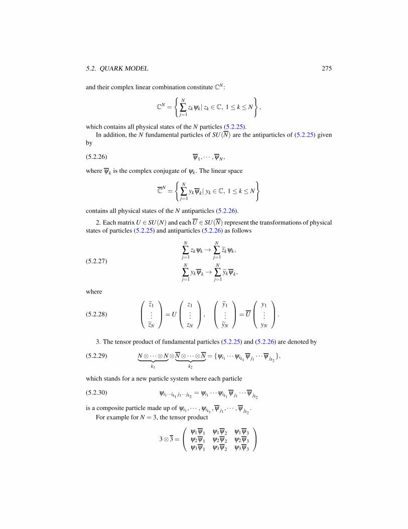
5.2. QUARK MODEL 275
and their complex linear combination constitute CN :
CN =
N
∑j=1
zkψk| zk ∈ C, 1 ≤ k ≤ N
,
which contains all physical states of the N particles (5.2.25).
In addition, the N fundamental particles of SU(N) are the antiparticles of (5.2.25) given
by
(5.2.26) ψ1, · · · ,ψN ,
where ψk is the complex conjugate of ψk. The linear space
CN=
N
∑j=1
ykψk| yk ∈ C, 1 ≤ k ≤ N
contains all physical states of the N antiparticles (5.2.26).
2. Each matrix U ∈ SU(N) and each U ∈ SU(N) represent the transformations of physical
states of particles (5.2.25) and antiparticles (5.2.26) as follows
(5.2.27)
N
∑j=1
zkψk →N
∑j=1
zkψk,
N
∑j=1
ykψk →N
∑j=1
ykψk,
where
(5.2.28)
z1
...
zN
=U
z1
...
zN
,
y1
...
yN
=U
y1
...
yN
.
3. The tensor product of fundamental particles (5.2.25) and (5.2.26) are denoted by
(5.2.29) N ⊗·· ·⊗N︸ ︷︷ ︸k1
⊗N ⊗·· ·⊗N︸ ︷︷ ︸k2
= ψi1 · · ·ψik1ψ j1
· · ·ψ jk2,
which stands for a new particle system where each particle
(5.2.30) ψi1···ik1j1··· jk2
= ψi1 · · ·ψik1ψ j1
· · ·ψ jk2
is a composite particle made up of ψi1 , · · · ,ψik1,ψ j1
, · · · ,ψ jk2.
For example for N = 3, the tensor product
3⊗ 3 =
ψ1ψ1 ψ1ψ2 ψ1ψ3
ψ2ψ1 ψ2ψ2 ψ2ψ3
ψ3ψ1 ψ3ψ2 ψ3ψ3
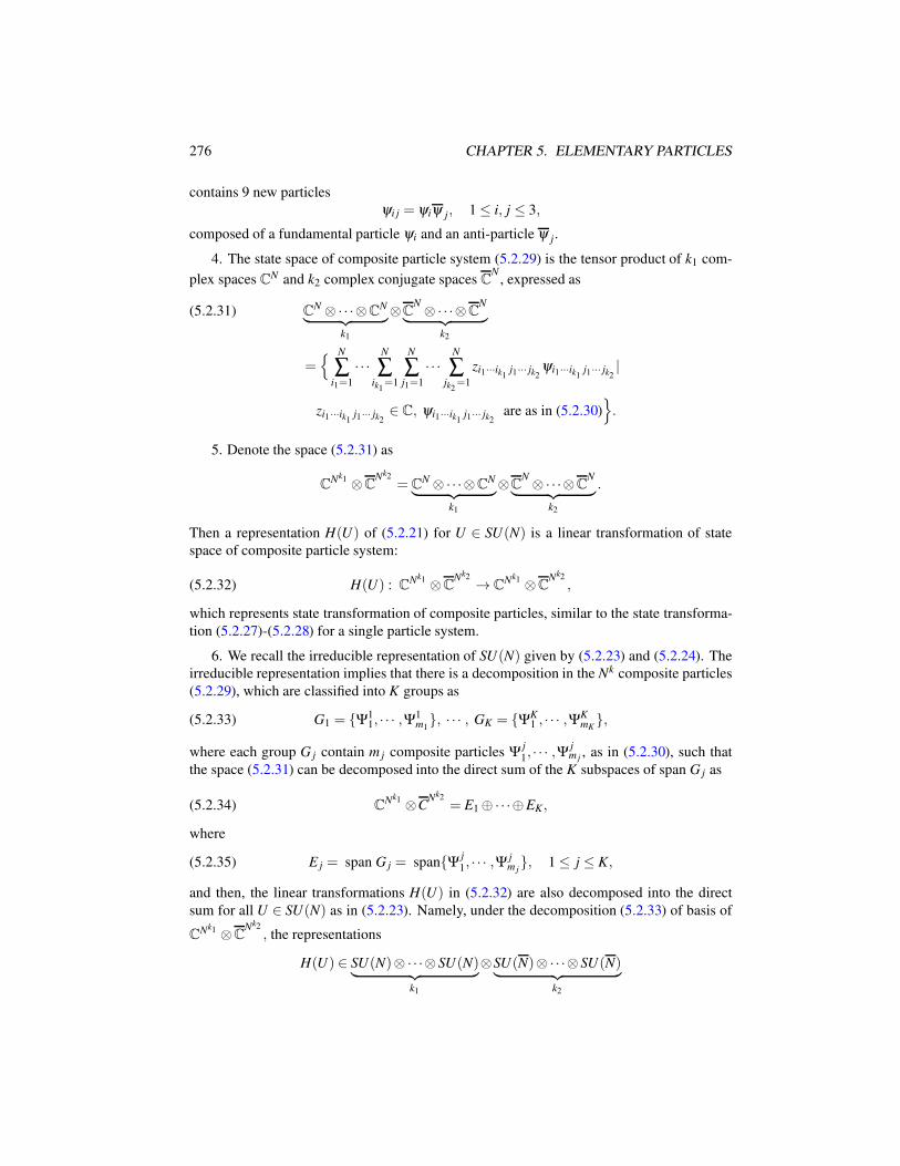
276 CHAPTER 5. ELEMENTARY PARTICLES
contains 9 new particles
ψi j = ψiψ j, 1 ≤ i, j ≤ 3,
composed of a fundamental particle ψi and an anti-particle ψ j.
4. The state space of composite particle system (5.2.29) is the tensor product of k1 com-
plex spaces CN and k2 complex conjugate spaces CN
, expressed as
CN ⊗·· ·⊗C
N
︸ ︷︷ ︸k1
⊗CN ⊗·· ·⊗C
N
︸ ︷︷ ︸k2
(5.2.31)
= N
∑i1=1
· · ·N
∑ik1
=1
N
∑j1=1
· · ·N
∑jk2
=1
zi1···ik1j1··· jk2
ψi1···ik1j1··· jk2
|
zi1···ik1j1··· jk2
∈ C, ψi1···ik1j1··· jk2
are as in (5.2.30).
5. Denote the space (5.2.31) as
CNk1 ⊗C
Nk2= C
N ⊗·· ·⊗CN
︸ ︷︷ ︸k1
⊗CN ⊗·· ·⊗C
N
︸ ︷︷ ︸k2
.
Then a representation H(U) of (5.2.21) for U ∈ SU(N) is a linear transformation of state
space of composite particle system:
(5.2.32) H(U) : CNk1 ⊗C
Nk2 → CNk1 ⊗C
Nk2
,
which represents state transformation of composite particles, similar to the state transforma-
tion (5.2.27)-(5.2.28) for a single particle system.
6. We recall the irreducible representation of SU(N) given by (5.2.23) and (5.2.24). The
irreducible representation implies that there is a decomposition in the Nk composite particles
(5.2.29), which are classified into K groups as
(5.2.33) G1 = Ψ11, · · · ,Ψ1
m1, · · · , GK = ΨK
1 , · · · ,ΨKmK
,
where each group G j contain m j composite particles Ψ j1, · · · ,Ψ
jm j
, as in (5.2.30), such that
the space (5.2.31) can be decomposed into the direct sum of the K subspaces of span G j as
(5.2.34) CNk1 ⊗C
Nk2= E1 ⊕·· ·⊕EK,
where
(5.2.35) E j = span G j = spanΨj1, · · · ,Ψ j
m j, 1 ≤ j ≤ K,
and then, the linear transformations H(U) in (5.2.32) are also decomposed into the direct
sum for all U ∈ SU(N) as in (5.2.23). Namely, under the decomposition (5.2.33) of basis of
CNk1 ⊗CNk2
, the representations
H(U) ∈ SU(N)⊗·· ·⊗ SU(N)︸ ︷︷ ︸k1
⊗SU(N)⊗·· ·⊗ SU(N)︸ ︷︷ ︸k2
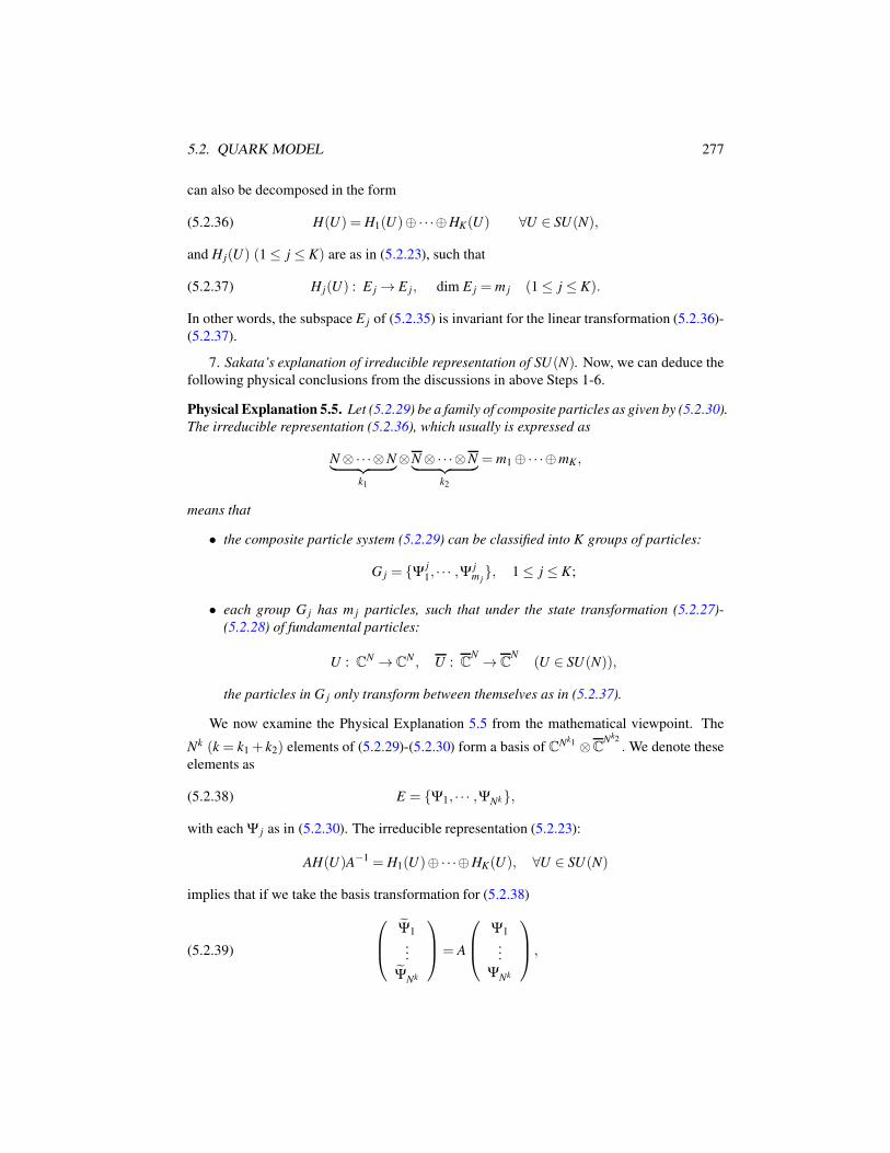
5.2. QUARK MODEL 277
can also be decomposed in the form
(5.2.36) H(U) = H1(U)⊕·· ·⊕HK(U) ∀U ∈ SU(N),
and H j(U) (1 ≤ j ≤ K) are as in (5.2.23), such that
(5.2.37) H j(U) : E j → E j, dim E j = m j (1 ≤ j ≤ K).
In other words, the subspace E j of (5.2.35) is invariant for the linear transformation (5.2.36)-
(5.2.37).
7. Sakata’s explanation of irreducible representation of SU(N). Now, we can deduce the
following physical conclusions from the discussions in above Steps 1-6.
Physical Explanation 5.5. Let (5.2.29) be a family of composite particles as given by (5.2.30).
The irreducible representation (5.2.36), which usually is expressed as
N ⊗·· ·⊗N︸ ︷︷ ︸k1
⊗N ⊗·· ·⊗N︸ ︷︷ ︸k2
= m1 ⊕·· ·⊕mK ,
means that
• the composite particle system (5.2.29) can be classified into K groups of particles:
G j = Ψ j1, · · · ,Ψ j
m j, 1 ≤ j ≤ K;
• each group G j has m j particles, such that under the state transformation (5.2.27)-
(5.2.28) of fundamental particles:
U : CN → C
N , U : CN → C
N(U ∈ SU(N)),
the particles in G j only transform between themselves as in (5.2.37).
We now examine the Physical Explanation 5.5 from the mathematical viewpoint. The
Nk (k = k1 + k2) elements of (5.2.29)-(5.2.30) form a basis of CNk1 ⊗CNk2
. We denote these
elements as
(5.2.38) E = Ψ1, · · · ,ΨNk,
with each Ψ j as in (5.2.30). The irreducible representation (5.2.23):
AH(U)A−1 = H1(U)⊕·· ·⊕HK(U), ∀U ∈ SU(N)
implies that if we take the basis transformation for (5.2.38)
(5.2.39)
Ψ1
...
ΨNk
= A
Ψ1
...
ΨNk
,
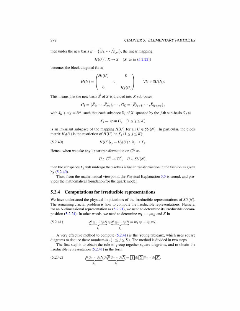
278 CHAPTER 5. ELEMENTARY PARTICLES
then under the new basis E = Ψ1, · · · ,ΨNk, the linear mapping
H(U) : X → X (X as in (5.2.22))
becomes the block diagonal form
H(U) =
H1(U) 0
. . .
0 HK(U)
∀U ∈ SU(N).
This means that the new basis E of X is divided into K sub-bases
G1 = E1, · · · , Em1, · · · , GK = EJK+1, · · · , EJk+mK
,
with JK +mK = NK , such that each subspace XJ of X , spanned by the j-th sub-basis G j as
X j = span G j (1 ≤ j ≤ K)
is an invariant subspace of the mapping H(U) for all U ∈ SU(N). In particular, the block
matrix H j(U) is the restriction of H(U) on X j (1 ≤ j ≤ K):
(5.2.40) H(U)|X j= H j(U) : X j → X j.
Hence, when we take any linear transformation on CN as
U : CN → C
N , U ∈ SU(N),
then the subspaces X j will undergo themselves a linear transformation in the fashion as given
by (5.2.40).
Thus, from the mathematical viewpoint, the Physical Explanation 5.5 is sound, and pro-
vides the mathematical foundation for the quark model.
5.2.4 Computations for irreducible representations
We have understood the physical implications of the irreducible representations of SU(N).The remaining crucial problem is how to compute the irreducible representations. Namely,
for an N-dimensional representation as (5.2.21), we need to determine its irreducible decom-
position (5.2.24). In other words, we need to determine m1, · · · ,mK and K in
(5.2.41) N ⊗·· ·⊗N︸ ︷︷ ︸k1
⊗N ⊗·· ·⊗N︸ ︷︷ ︸k2
= m1 ⊕·· ·⊕mK.
A very effective method to compute (5.2.41) is the Young tableaux, which uses square
diagrams to deduce these numbers m j (1 ≤ j ≤ K). The method is divided in two steps.
The first step is to obtain the rule to group together square diagrams, and to obtain the
irreducible representation (5.2.41) in the form
(5.2.42) N ⊗·· ·⊗N︸ ︷︷ ︸k1
⊗N ⊗·· ·⊗N︸ ︷︷ ︸k2
= 1 ⊕ 2 ⊕·· ·⊕ K .
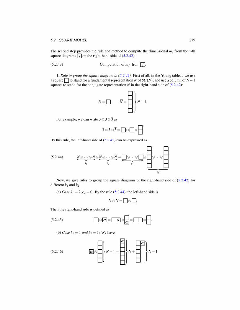
5.2. QUARK MODEL 279
The second step provides the rule and method to compute the dimensional m j from the j-th
square diagrams j on the right-hand side of (5.2.42):
(5.2.43) Computation of m j from j .
1. Rule to group the square diagram in (5.2.42). First of all, in the Young tableau we use
a square to stand for a fundamental representation N of SU(N), and use a column of N−1
squares to stand for the conjugate representation N in the right-hand side of (5.2.42):
N = , N =
N − 1.
For example, we can write 3⊗ 3⊗ 3 as
3⊗ 3⊗ 3= ⊗ ⊗ .
By this rule, the left-hand side of (5.2.42) can be expressed as
(5.2.44) N ⊗·· ·⊗N︸ ︷︷ ︸k1
⊗N ⊗·· ·⊗N︸ ︷︷ ︸k2
= ⊗·· ·⊗︸ ︷︷ ︸k1
⊗ ⊗·· ·⊗
︸ ︷︷ ︸k2
Now, we give rules to group the square diagrams of the right-hand side of (5.2.42) for
different k1 and k2.
(a) Case k1 = 2,k2 = 0: By the rule (5.2.44), the left-hand side is
N ⊗N = ⊗ .
Then the right-hand side is defined as
(5.2.45) ⊗ α = α ⊕α
= ⊕ .
(b) Case k1 = 1 and k2 = 1: We have
(5.2.46) α ⊗
N − 1 =
α
N +
α
N − 1
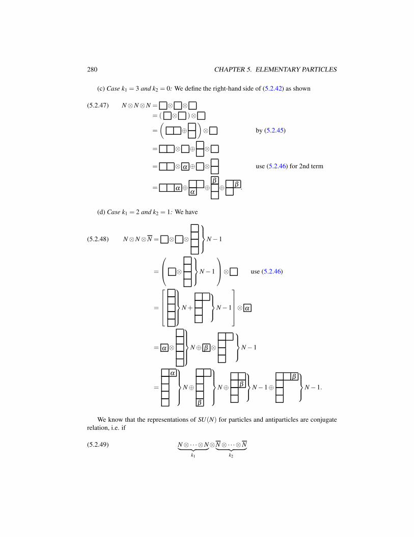
280 CHAPTER 5. ELEMENTARY PARTICLES
(c) Case k1 = 3 and k2 = 0: We define the right-hand side of (5.2.42) as shown
N ⊗N ⊗N = ⊗ ⊗(5.2.47)
= ( ⊗ )⊗
=
(⊕
)⊗ by (5.2.45)
= ⊗ ⊕ ⊗
= ⊗ α ⊕ ⊗ use (5.2.46) for 2nd term
= α ⊕α
⊕β
⊕ β .
(d) Case k1 = 2 and k2 = 1: We have
N ⊗N ⊗N = ⊗ ⊗
N − 1(5.2.48)
=
⊗
N − 1
⊗ use (5.2.46)
=
N +
N − 1
⊗ α
= α ⊗
N ⊕ β ⊗
N − 1
=
α
N ⊕
β
N ⊕ β
N − 1⊕β
N − 1.
We know that the representations of SU(N) for particles and antiparticles are conjugate
relation, i.e. if
(5.2.49) N ⊗·· ·⊗N︸ ︷︷ ︸k1
⊗N ⊗·· ·⊗N︸ ︷︷ ︸k2
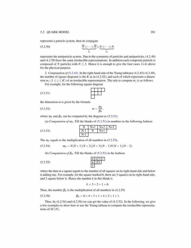
5.2. QUARK MODEL 281
represents a particle system, then its conjugate
(5.2.50) N ⊗·· ·⊗N︸ ︷︷ ︸k1
⊗N ⊗·· ·⊗N︸ ︷︷ ︸k2
represents the antiparticle system. Due to the symmetry of particles and antiparticles, (4.2.49)
and (4.2.50) have the same irreducible representations. In addition each composite particle is
composed of N particles with N ≤ 3. Hence it is enough to give the four cases 1)-4) above
for the physical purpose.
2. Computation of (5.2.43). In the right-hand side of the Young tableaux (4.2.45)-(4.2.48),
the number of square diagrams is the K as in (4.2.42), and each of which represents a dimen-
sion m j (1 ≤ j ≤ K) of an irreducible representation. The rule to compute m j is as follows.
For example, for the following square diagram
(5.2.51)
the dimension m is given by the formula
(5.2.52) m =αN
βN
,
where αN and βN can be computed by the diagram as (5.2.51).
(a) Computation of αN . Fill the blanks of (5.2.51) in numbers in the following fashion:
(5.2.53)
N N+1 N+2 N+2
N-1 N N+1
N-2
The αN equals to the multiplication of all numbers in (5.2.53),
(5.2.54) αN = N(N + 1)(N + 2)(N + 3)(N − 1)N(N + 1)(N − 2).
(b) Computation of βN . Fill the blanks of (5.2.51) in the fashion:
(5.2.55)6 4 3 14 2 11
where the data in a square equals to the number of all squares on its right-hand side and below
it adding one. For example, for the square marked 6, there are 3 squares on its right-hand side,
and 2 square below it. Hence the number k in this blank is
k = 3+ 2+ 1= 6.
Then, the number βN is the multiplication of all numbers in (4.2.55)
(5.2.56) βN = 6× 4× 3× 1×4×2×1×1.
Thus, by (4.2.54) and (4.2.56) we can get the value of (4.2.52). In the following, we give
a few examples to show how to use the Young tableau to compute the irreducible representa-
tions of SU(N).
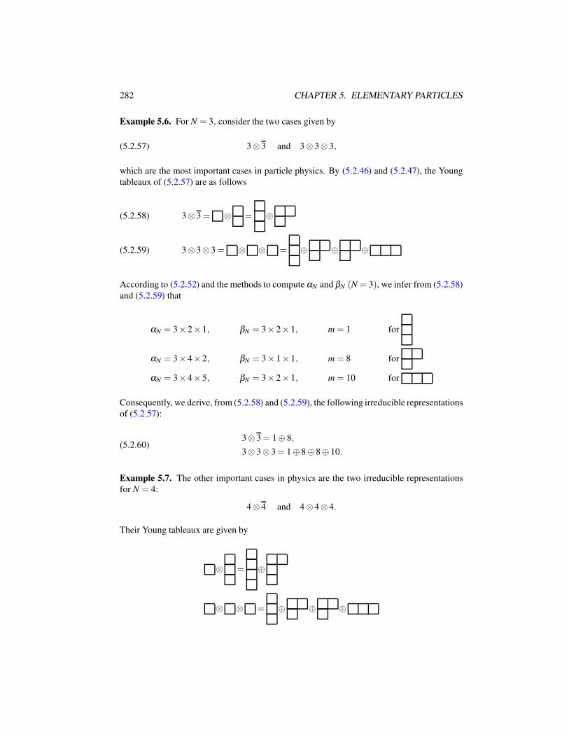
282 CHAPTER 5. ELEMENTARY PARTICLES
Example 5.6. For N = 3, consider the two cases given by
(5.2.57) 3⊗ 3 and 3⊗ 3⊗ 3,
which are the most important cases in particle physics. By (5.2.46) and (5.2.47), the Young
tableaux of (5.2.57) are as follows
3⊗ 3 = ⊗ = ⊕(5.2.58)
3⊗ 3⊗ 3= ⊗ ⊗ = ⊕ ⊕ ⊕(5.2.59)
According to (5.2.52) and the methods to compute αN and βN (N = 3), we infer from (5.2.58)
and (5.2.59) that
αN = 3× 2× 1, βN = 3× 2× 1, m = 1 for
αN = 3× 4× 2, βN = 3× 1× 1, m = 8 for
αN = 3× 4× 5, βN = 3× 2× 1, m = 10 for
Consequently, we derive, from (5.2.58) and (5.2.59), the following irreducible representations
of (5.2.57):
(5.2.60)3⊗ 3 = 1⊕ 8,
3⊗ 3⊗ 3= 1⊕ 8⊕ 8⊕ 10.
Example 5.7. The other important cases in physics are the two irreducible representations
for N = 4:
4⊗ 4 and 4⊗ 4⊗ 4.
Their Young tableaux are given by
⊗ = ⊕
⊗ ⊗ = ⊕ ⊕ ⊕
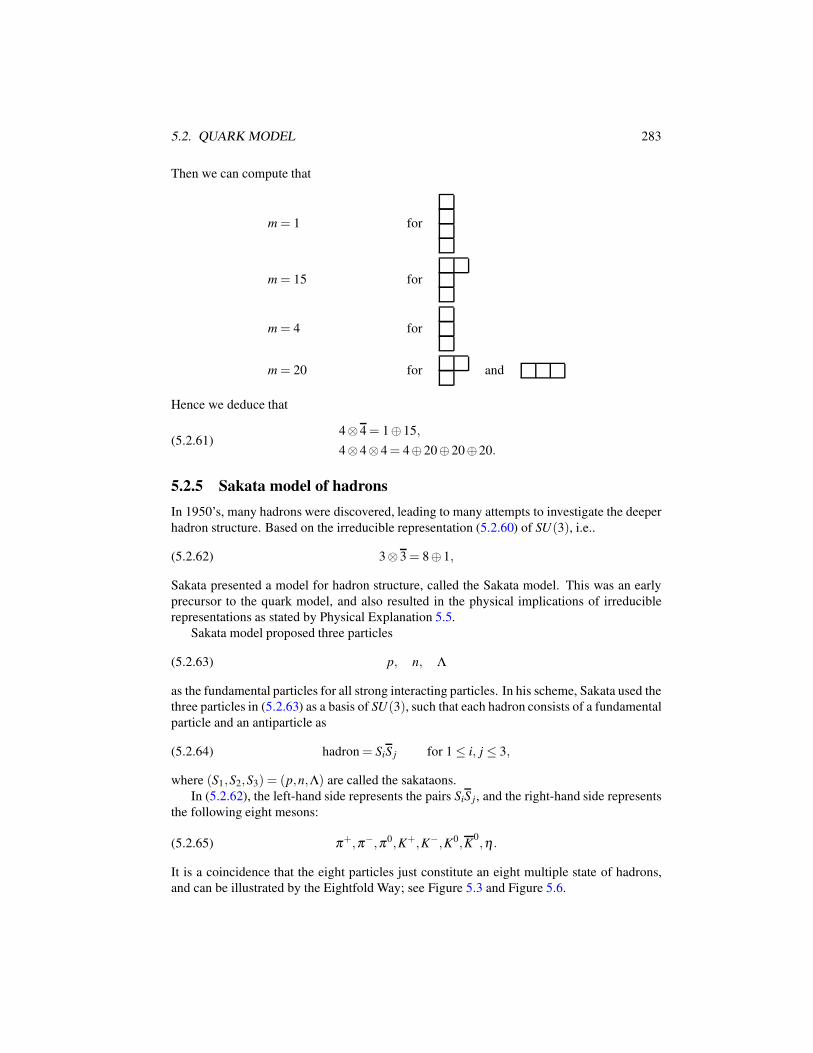
5.2. QUARK MODEL 283
Then we can compute that
m = 1 for
m = 15 for
m = 4 for
m = 20 for and
Hence we deduce that
(5.2.61)4⊗ 4 = 1⊕ 15,
4⊗ 4⊗ 4= 4⊕ 20⊕ 20⊕20.
5.2.5 Sakata model of hadrons
In 1950’s, many hadrons were discovered, leading to many attempts to investigate the deeper
hadron structure. Based on the irreducible representation (5.2.60) of SU(3), i.e..
(5.2.62) 3⊗ 3 = 8⊕ 1,
Sakata presented a model for hadron structure, called the Sakata model. This was an early
precursor to the quark model, and also resulted in the physical implications of irreducible
representations as stated by Physical Explanation 5.5.
Sakata model proposed three particles
(5.2.63) p, n, Λ
as the fundamental particles for all strong interacting particles. In his scheme, Sakata used the
three particles in (5.2.63) as a basis of SU(3), such that each hadron consists of a fundamental
particle and an antiparticle as
(5.2.64) hadron = SiS j for 1 ≤ i, j ≤ 3,
where (S1,S2,S3) = (p,n,Λ) are called the sakataons.
In (5.2.62), the left-hand side represents the pairs SiS j, and the right-hand side represents
the following eight mesons:
(5.2.65) π+,π−,π0,K+,K−,K0,K0,η .
It is a coincidence that the eight particles just constitute an eight multiple state of hadrons,
and can be illustrated by the Eightfold Way; see Figure 5.3 and Figure 5.6.
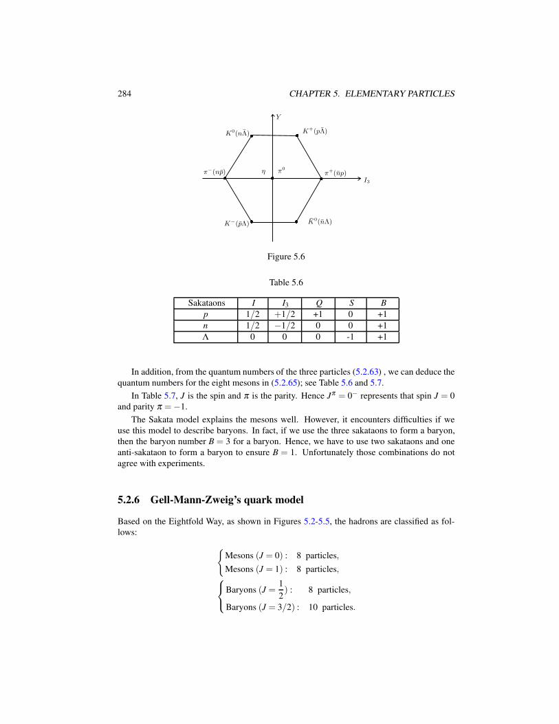
284 CHAPTER 5. ELEMENTARY PARTICLES
Y
K+(pΛ)
π+(np)I3
K0(nΛ)K−(pΛ)
π−(np) η π0
K0(nΛ)
Figure 5.6
Table 5.6
Sakataons I I3 Q S B
p 1/2 +1/2 +1 0 +1
n 1/2 −1/2 0 0 +1
Λ 0 0 0 -1 +1
In addition, from the quantum numbers of the three particles (5.2.63) , we can deduce the
quantum numbers for the eight mesons in (5.2.65); see Table 5.6 and 5.7.
In Table 5.7, J is the spin and π is the parity. Hence Jπ = 0− represents that spin J = 0
and parity π =−1.
The Sakata model explains the mesons well. However, it encounters difficulties if we
use this model to describe baryons. In fact, if we use the three sakataons to form a baryon,
then the baryon number B = 3 for a baryon. Hence, we have to use two sakataons and one
anti-sakataon to form a baryon to ensure B = 1. Unfortunately those combinations do not
agree with experiments.
5.2.6 Gell-Mann-Zweig’s quark model
Based on the Eightfold Way, as shown in Figures 5.2-5.5, the hadrons are classified as fol-
lows:
Mesons (J = 0) : 8 particles,
Mesons (J = 1) : 8 particles,
Baryons (J =1
2) : 8 particles,
Baryons (J = 3/2) : 10 particles.
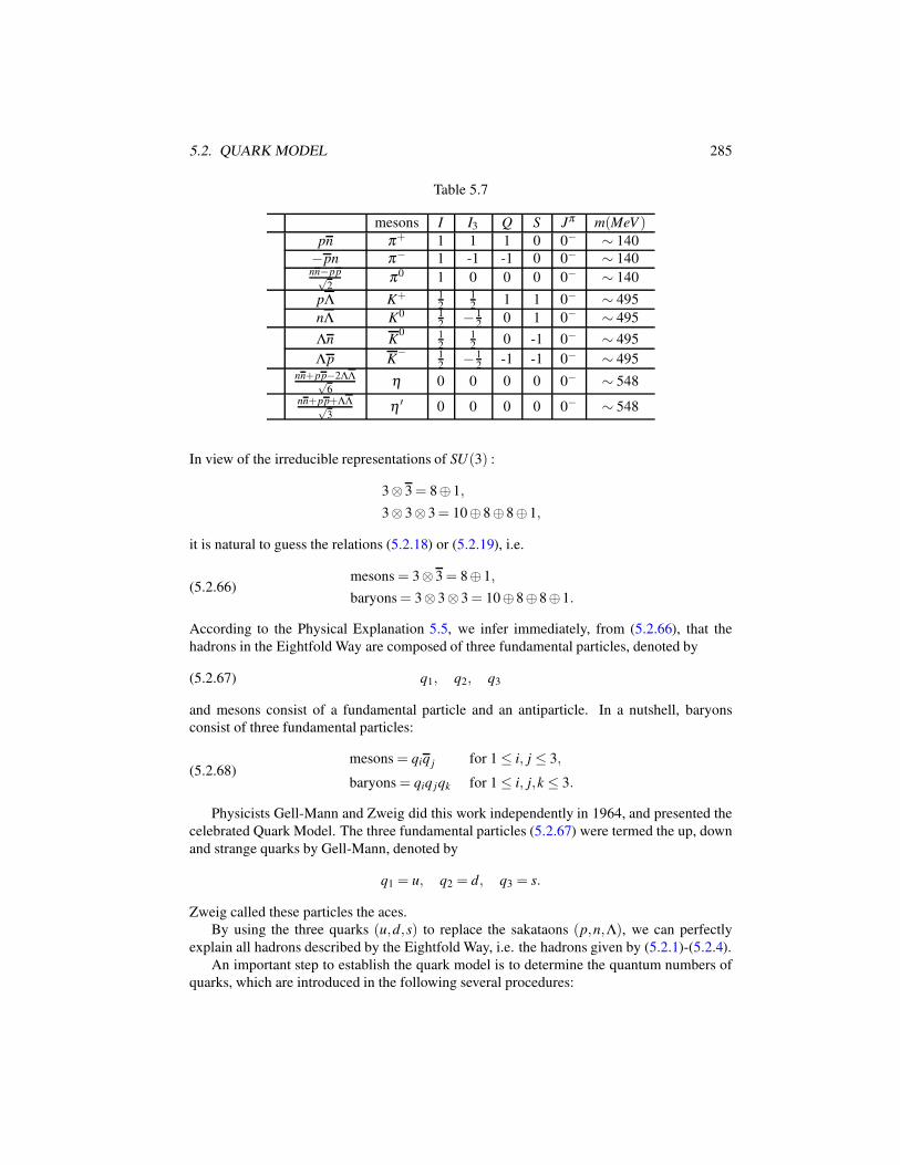
5.2. QUARK MODEL 285
Table 5.7
mesons I I3 Q S Jπ m(MeV )pn π+ 1 1 1 0 0− ∼ 140
−pn π− 1 -1 -1 0 0− ∼ 140nn−pp√
2π0 1 0 0 0 0− ∼ 140
pΛ K+ 12
12
1 1 0− ∼ 495
nΛ K0 12
− 12
0 1 0− ∼ 495
Λn K0 1
212
0 -1 0− ∼ 495
Λp K− 1
2− 1
2-1 -1 0− ∼ 495
nn+pp−2ΛΛ√6
η 0 0 0 0 0− ∼ 548
nn+pp+ΛΛ√3
η ′ 0 0 0 0 0− ∼ 548
In view of the irreducible representations of SU(3) :
3⊗ 3 = 8⊕ 1,
3⊗ 3⊗ 3= 10⊕ 8⊕ 8⊕ 1,
it is natural to guess the relations (5.2.18) or (5.2.19), i.e.
(5.2.66)mesons = 3⊗ 3 = 8⊕ 1,
baryons = 3⊗ 3⊗ 3= 10⊕ 8⊕ 8⊕1.
According to the Physical Explanation 5.5, we infer immediately, from (5.2.66), that the
hadrons in the Eightfold Way are composed of three fundamental particles, denoted by
(5.2.67) q1, q2, q3
and mesons consist of a fundamental particle and an antiparticle. In a nutshell, baryons
consist of three fundamental particles:
(5.2.68)mesons = qiq j for 1 ≤ i, j ≤ 3,
baryons = qiq jqk for 1 ≤ i, j,k ≤ 3.
Physicists Gell-Mann and Zweig did this work independently in 1964, and presented the
celebrated Quark Model. The three fundamental particles (5.2.67) were termed the up, down
and strange quarks by Gell-Mann, denoted by
q1 = u, q2 = d, q3 = s.
Zweig called these particles the aces.
By using the three quarks (u,d,s) to replace the sakataons (p,n,Λ), we can perfectly
explain all hadrons described by the Eightfold Way, i.e. the hadrons given by (5.2.1)-(5.2.4).
An important step to establish the quark model is to determine the quantum numbers of
quarks, which are introduced in the following several procedures:
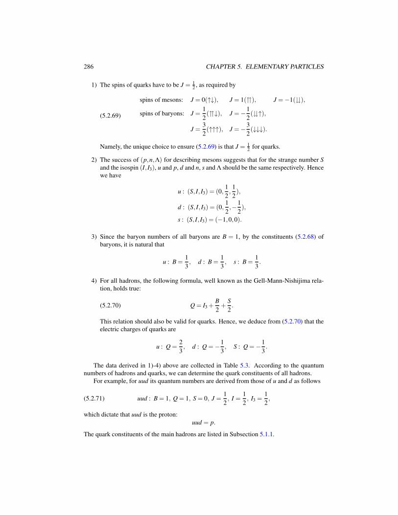
286 CHAPTER 5. ELEMENTARY PARTICLES
1) The spins of quarks have to be J = 12, as required by
(5.2.69)
spins of mesons: J = 0(↑↓), J = 1(), J =−1(),
spins of baryons: J =1
2(↓), J =−1
2(↑),
J =3
2(↑↑↑), J =−3
2(↓↓↓).
Namely, the unique choice to ensure (5.2.69) is that J = 12
for quarks.
2) The success of (p,n,Λ) for describing mesons suggests that for the strange number S
and the isospin (I, I3), u and p, d and n, s and Λ should be the same respectively. Hence
we have
u : (S, I, I3) = (0,1
2,
1
2),
d : (S, I, I3) = (0,1
2,−1
2),
s : (S, I, I3) = (−1,0,0).
3) Since the baryon numbers of all baryons are B = 1, by the constituents (5.2.68) of
baryons, it is natural that
u : B =1
3, d : B =
1
3, s : B =
1
3.
4) For all hadrons, the following formula, well known as the Gell-Mann-Nishijima rela-
tion, holds true:
(5.2.70) Q = I3 +B
2+
S
2.
This relation should also be valid for quarks. Hence, we deduce from (5.2.70) that the
electric charges of quarks are
u : Q =2
3, d : Q =−1
3, S : Q =−1
3.
The data derived in 1)-4) above are collected in Table 5.3. According to the quantum
numbers of hadrons and quarks, we can determine the quark constituents of all hadrons.
For example, for uud its quantum numbers are derived from those of u and d as follows
(5.2.71) uud : B = 1, Q = 1, S = 0, J =1
2, I =
1
2, I3 =
1
2,
which dictate that uud is the proton:
uud = p.
The quark constituents of the main hadrons are listed in Subsection 5.1.1.
5.3. WEAKTON MODEL OF ELEMENTARY PARTICLES 287
In 1974, Ting and Richter discovered independently J/ψ particle, which implies the ex-
istence of a new quark, named as the c quark. Thus, the quark family then was extended to
four members:
u,d,s,c.
As fundamental particles of SU(4), the irreducible representations (5.2.61), written as
(5.2.72)4⊗ 4 = 15⊕ 1,4⊗ 4⊗ 4= 20⊕ 20⊕ 20⊕4
suggest that the meson groups with 8 particles should be extended to 15 particles, and the
baryons be extended to 20 particles in a group. The extended group of mesons with 15
particles has been verified, which is given by
π±, π0, K±, K0, K0, η , η ′, D0, D0, D±, D±
s .
However, the 20 baryons corresponding to the irreducible representation (5.2.72) have not
been discovered now.
Up to now, the quark family has six members:
u,d,s,c,b, t.
Their irreducible representation is given by
(5.2.73)6⊗ 6 = 35⊕ 1,6⊗ 6⊗ 6= 70⊕ 70⊕ 56⊕20.
The classification scheme corresponding to (5.2.73) does not seem to be realistic. The irre-
ducible representation of SU(N) is only a phenomenological theory in elementary particle
physics.
5.3 Weakton Model of Elementary Particles
5.3.1 Decay means the interior structure
As we addressed in Section 5.1.3, all charged leptons, quarks and mediators can undergo
decay as follows:
1) Charged lepton radiation and decay:
e− → e−+ γ,
µ− → e−+νe +νµ ,(5.3.1)
τ− → µ−+νµ +ντ .
2) Quark decay:
d → u+ e−+νe,
s → d + γ,(5.3.2)
c → d+ s+ u.
288 CHAPTER 5. ELEMENTARY PARTICLES
3) Mediator decay:
2γ → e++ e−,
W± → l±+ν l± ,(5.3.3)
Z → l++ l−,
where l± are the charged leptons.
All leptons, quarks and mediators are currently regarded as elementary particles. How-
ever, the decays in (5.3.1)-(5.3.3) show that these particles must have an interior structure,
and consequently they should be considered as composite particles rather than elementary
particles:
Decay Means Interior Structure.
5.3.2 Theoretical foundations for the weakton model
Subatomic decays and electron radiations indicate that there must be interior structure for
charged leptons, quarks and mediators. The main objective of this section is to propose an
elementary particle model, which we call weakton model, based on the weak and strong
interaction theories developed in the last chapter.
Angular momentum rule
It is known that the dynamic behavior of a particle is described by the Dirac equations:
(5.3.4) ih∂ψ
∂ t= Hψ ,
where ψ = (ψ1,ψ2,ψ3,ψ4)T is the Dirac spinor, H is the Hamiltonian:
(5.3.5) H =−ihc(αk∂k)+mc2α0 +V(x),
V is the potential energy, αk (1 ≤ k ≤ 3) are the matrices as given by (2.2.48), and α0 is the
matrix as
α0 =
(I 0
0 −I
), I =
(1 0
0 1
).
By the conservation laws in quantum mechanics, if an Hermitian operator L commutes with
H in (5.3.5):
LH = HL,
then the physical quantity L is conserved.
Consider the total angular momentum ~J of a particle as
~J =~L+ s~S,
where~L is the orbital angular momentum
~L =~r×~p, ~p =−ih∇,
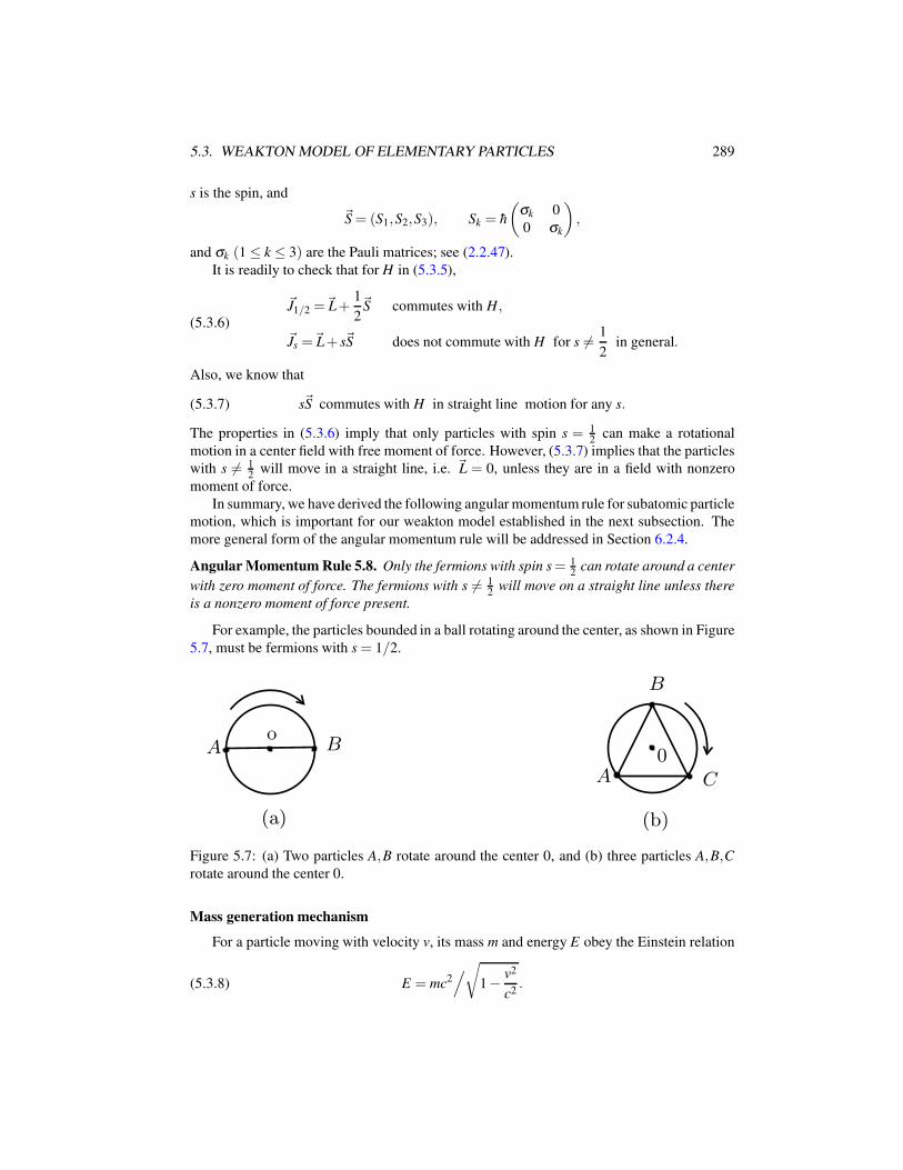
5.3. WEAKTON MODEL OF ELEMENTARY PARTICLES 289
s is the spin, and
~S = (S1,S2,S3), Sk = h
(σk 0
0 σk
),
and σk (1 ≤ k ≤ 3) are the Pauli matrices; see (2.2.47).
It is readily to check that for H in (5.3.5),
(5.3.6)
~J1/2 =~L+1
2~S commutes with H,
~Js =~L+ s~S does not commute with H for s 6= 1
2in general.
Also, we know that
(5.3.7) s~S commutes with H in straight line motion for any s.
The properties in (5.3.6) imply that only particles with spin s = 12
can make a rotational
motion in a center field with free moment of force. However, (5.3.7) implies that the particles
with s 6= 12
will move in a straight line, i.e. ~L = 0, unless they are in a field with nonzero
moment of force.
In summary, we have derived the following angular momentum rule for subatomic particle
motion, which is important for our weakton model established in the next subsection. The
more general form of the angular momentum rule will be addressed in Section 6.2.4.
Angular Momentum Rule 5.8. Only the fermions with spin s= 12
can rotate around a center
with zero moment of force. The fermions with s 6= 12
will move on a straight line unless there
is a nonzero moment of force present.
For example, the particles bounded in a ball rotating around the center, as shown in Figure
5.7, must be fermions with s = 1/2.
A Bo
(a)
A
B
0
(b)
C
Figure 5.7: (a) Two particles A,B rotate around the center 0, and (b) three particles A,B,Crotate around the center 0.
Mass generation mechanism
For a particle moving with velocity v, its mass m and energy E obey the Einstein relation
(5.3.8) E = mc2/√
1− v2
c2.
290 CHAPTER 5. ELEMENTARY PARTICLES
Usually, we regard m as a static mass which is fixed, and energy is a function of velocity v.
Now, taking an opposite viewpoint, we regard energy E as fixed, mass m as a function of
velocity v, and the relation (5.3.8) is rewritten as
(5.3.9) m =
√1− v2
c2
E
c2.
Thus, (5.3.9) means that a particle with an intrinsic energy E has zero mass m = 0 if it moves
at the speed of light v = c, and will possess nonzero mass if it moves with a velocity v < c.
All particles including photons can only travel at the speed sufficiently close to the speed
of light. Based on this viewpoint, we can think that if a particle moving at the speed of light
(approximately) is decelerated by an interaction force ~F , obeying
d~P
dt=
√1− v2
c2~F ,
then this massless particle will generate mass at the instant. In particular, by this mass gener-
ation mechanism, several massless particles can yield a massive particle if they are bound in
a small ball, and rotate at velocities less than the speed of light.
Interaction charges
In the unified field model introduced in the last chapter, we derived that both weak and
strong interactions possess charges, as for gravity and electromagnetism; see Section 4.3.4:
(5.3.10)
gravitation: mass charge m,
electromagnetism: electric charge e,
weak interaction: weak charge gw,
strong interaction: strong charge gs.
If Φ is a charge potential corresponding to an interaction, then the interacting force generated
by its charge g is given by
F =−g∇Φ,
where ∇ is the spatial gradient operator.
It is very crucial to introduce both weak and strong interaction charges for us to develop
the weakton model. The charges in (5.3.10) possess the following physical properties:
1) Electric charge Qe, weak charge Qw, strong charge Qs are conservative. The energy
is a conserved quantity, but the mass M is not a conserved quantity due to the mass
generation mechanism as mentioned in (5.3.9).
2) There is no interacting force between two particles without common charges. For
example, if a particle A possesses no strong charge, then there is no strong interacting
force between A and any other particles.
3) Only the electric charge e can take both positive and negative values, and other charges
take only nonnegative values.
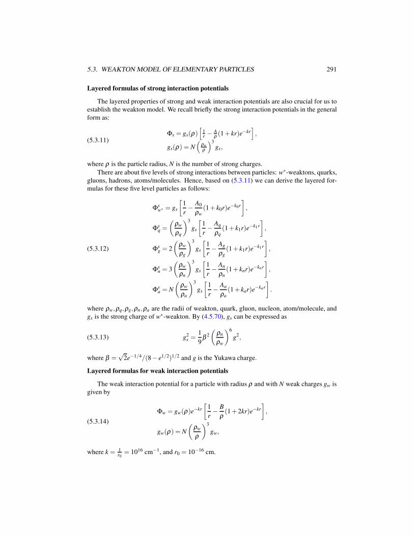
5.3. WEAKTON MODEL OF ELEMENTARY PARTICLES 291
Layered formulas of strong interaction potentials
The layered properties of strong and weak interaction potentials are also crucial for us to
establish the weakton model. We recall briefly the strong interaction potentials in the general
form as:
(5.3.11)Φs = gs(ρ)
[1r− A
ρ (1+ kr)e−kr],
gs(ρ) = N
(ρw
ρ
)3
gs,
where ρ is the particle radius, N is the number of strong charges.
There are about five levels of strong interactions between particles: w∗-weaktons, quarks,
gluons, hadrons, atoms/molecules. Hence, based on (5.3.11) we can derive the layered for-
mulas for these five level particles as follows:
(5.3.12)
Φsw∗ = gs
[1
r− A0
ρw
(1+ k0r)e−k0r
],
Φsq =
(ρw
ρq
)3
gs
[1
r− Aq
ρq
(1+ k1r)e−k1r
],
Φsg = 2
(ρw
ρg
)3
gs
[1
r− Ag
ρg
(1+ k1r)e−k1r
],
Φsn = 3
(ρw
ρn
)3
gs
[1
r− An
ρn
(1+ knr)e−knr
],
Φsa = N
(ρw
ρa
)3
gs
[1
r− Aa
ρa
(1+ kar)e−kar
].
where ρw,ρq,ρg,ρn,ρa are the radii of weakton, quark, gluon, nucleon, atom/molecule, and
gs is the strong charge of w∗-weakton. By (4.5.70), gs can be expressed as
(5.3.13) g2s =
1
9β 2
(ρn
ρw
)6
g2,
where β =√
2e−1/4/(8− e1/2)1/2 and g is the Yukawa charge.
Layered formulas for weak interaction potentials
The weak interaction potential for a particle with radius ρ and with N weak charges gw is
given by
(5.3.14)
Φw = gw(ρ)e−kr
[1
r− B
ρ(1+ 2kr)e−kr
],
gw(ρ) = N
(ρw
ρ
)3
gw,
where k = 1r0= 1016 cm−1, and r0 = 10−16 cm.
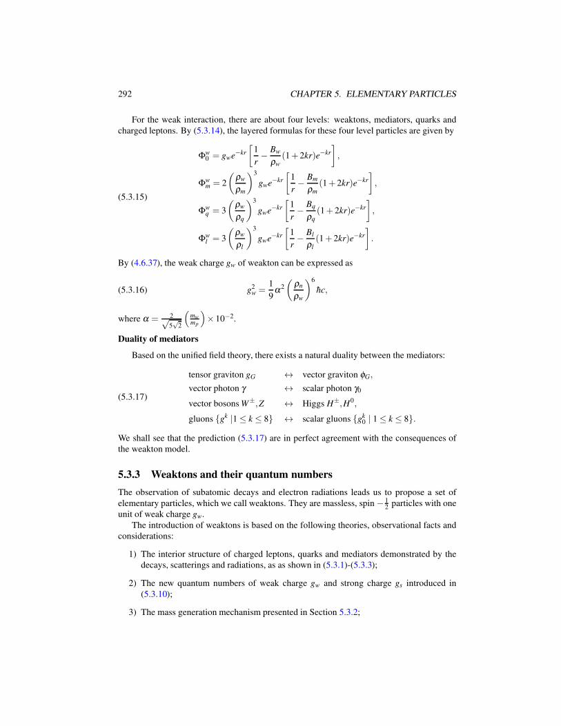
292 CHAPTER 5. ELEMENTARY PARTICLES
For the weak interaction, there are about four levels: weaktons, mediators, quarks and
charged leptons. By (5.3.14), the layered formulas for these four level particles are given by
(5.3.15)
Φw0 = gwe−kr
[1
r− Bw
ρw
(1+ 2kr)e−kr
],
Φwm = 2
(ρw
ρm
)3
gwe−kr
[1
r− Bm
ρm
(1+ 2kr)e−kr
],
Φwq = 3
(ρw
ρq
)3
gwe−kr
[1
r− Bq
ρq
(1+ 2kr)e−kr
],
Φwl = 3
(ρw
ρl
)3
gwe−kr
[1
r− Bl
ρl
(1+ 2kr)e−kr
].
By (4.6.37), the weak charge gw of weakton can be expressed as
(5.3.16) g2w =
1
9α2
(ρn
ρw
)6
hc,
where α = 2√5√
2
(mwmp
)× 10−2.
Duality of mediators
Based on the unified field theory, there exists a natural duality between the mediators:
(5.3.17)
tensor graviton gG ↔ vector graviton φG,
vector photon γ ↔ scalar photon γ0
vector bosons W±,Z ↔ Higgs H±,H0,
gluons gk |1 ≤ k ≤ 8 ↔ scalar gluons gk0 | 1 ≤ k ≤ 8.
We shall see that the prediction (5.3.17) are in perfect agreement with the consequences of
the weakton model.
5.3.3 Weaktons and their quantum numbers
The observation of subatomic decays and electron radiations leads us to propose a set of
elementary particles, which we call weaktons. They are massless, spin − 12
particles with one
unit of weak charge gw.
The introduction of weaktons is based on the following theories, observational facts and
considerations:
1) The interior structure of charged leptons, quarks and mediators demonstrated by the
decays, scatterings and radiations, as as shown in (5.3.1)-(5.3.3);
2) The new quantum numbers of weak charge gw and strong charge gs introduced in
(5.3.10);
3) The mass generation mechanism presented in Section 5.3.2;
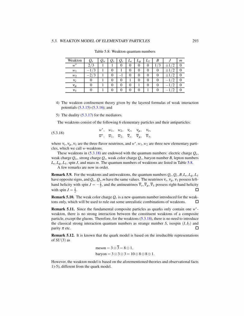
5.3. WEAKTON MODEL OF ELEMENTARY PARTICLES 293
Table 5.8: Weakton quantum numbers
Weakton Qe Qw Qs Qc Le Lµ Lτ B J m
w∗ 2/3 1 1 0 0 0 0 1/3 ±1/2 0
w1 −1/3 1 0 1 0 0 0 0 ±1/2 0
w2 −2/3 1 0 -1 0 0 0 0 ±1/2 0
νe 0 1 0 0 1 0 0 0 −1/2 0
νµ 0 1 0 0 0 1 0 0 −1/2 0
ντ 0 1 0 0 0 0 1 0 −1/2 0
4) The weakton confinement theory given by the layered formulas of weak interaction
potentials (5.3.15)-(5.3.16); and
5) The duality (5.3.17) for the mediators.
The weaktons consist of the following 6 elementary particles and their antiparticles:
(5.3.18)w∗, w1, w2, νe, νµ , ντ ,
w∗, w1, w2, νe, νµ , ντ ,
where νe,νµ ,ντ are the three flavor neutrinos, and w∗,w1,w2 are three new elementary parti-
cles, which we call w-weaktons.
These weaktons in (5.3.18) are endowed with the quantum numbers: electric charge Qe,
weak charge Qw, strong charge Qs, weak color charge Qc, baryon number B, lepton numbers
Le,Lµ ,Lτ , spin J, and mass m. The quantum numbers of weaktons are listed in Table 5.8.
A few remarks are now in order.
Remark 5.9. For the weaktons and antiweaktons, the quantum numbers Qe,Qc,B,Le,Lµ ,Lτ
have opposite signs, and Qw,Qs,m have the same values. The neutrinos νe,νµ ,ντ possess left-
hand helicity with spin J = − 12, and the antineutrinos νe,νµ ,ντ possess right-hand helicity
with spin J = 12.
Remark 5.10. The weak color charge Qc is a new quantum number introduced for the weak-
tons only, which will be used to rule out some unrealistic combinations of weaktons.
Remark 5.11. Since the fundamental composite particles as quarks only contain one w∗-
weakton, there is no strong interaction between the constituent weaktons of a composite
particle, except the gluons. Therefore, for the weaktons (5.3.18), there is no need to introduce
the classical strong interaction quantum numbers as strange number S, isospin (I, I3) and
parity π etc.
Remark 5.12. It is known that the quark model is based on the irreducible representations
of SU(3) as
meson = 3⊗ 3 = 8⊕ 1,
baryon = 3⊗ 3⊗ 3= 10⊕ 8⊕ 8⊕ 1.
However, the weakton model is based on the aforementioned theories and observational facts
1)-5), different from the quark model.
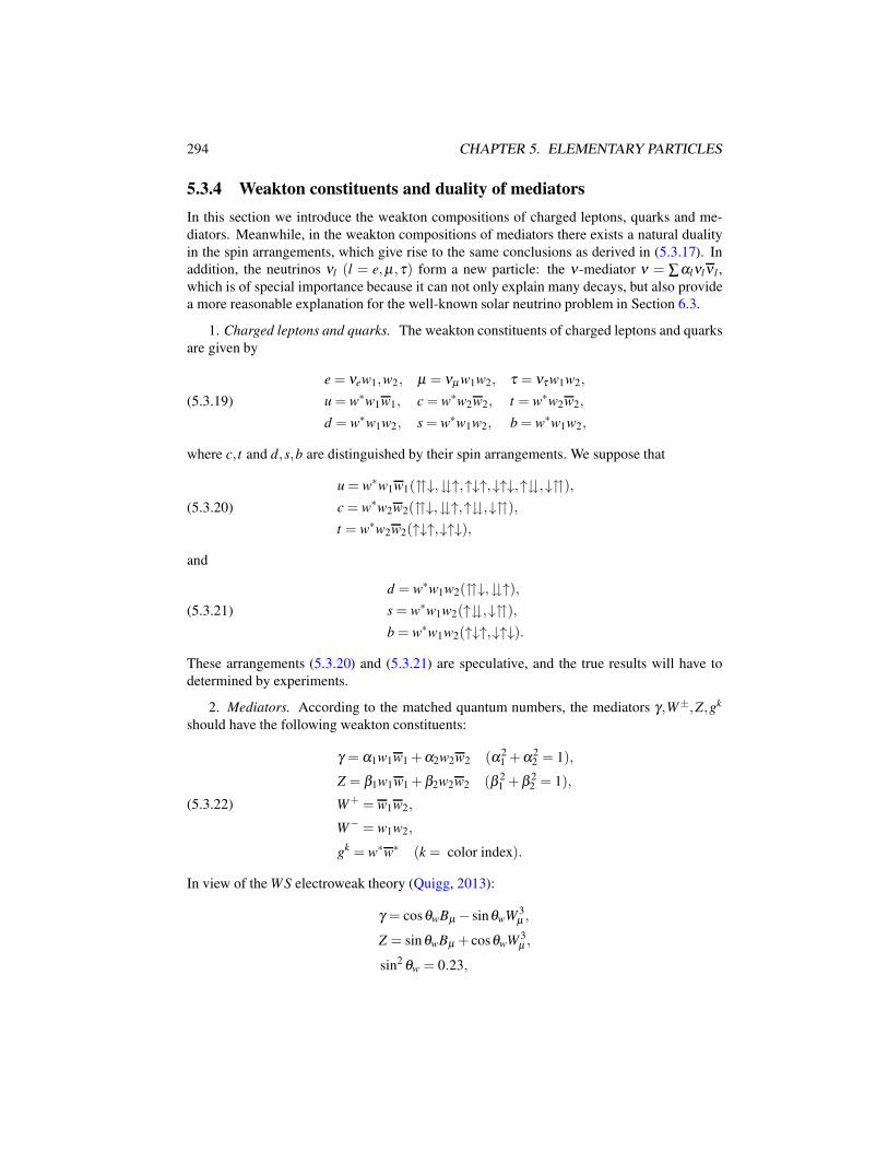
294 CHAPTER 5. ELEMENTARY PARTICLES
5.3.4 Weakton constituents and duality of mediators
In this section we introduce the weakton compositions of charged leptons, quarks and me-
diators. Meanwhile, in the weakton compositions of mediators there exists a natural duality
in the spin arrangements, which give rise to the same conclusions as derived in (5.3.17). In
addition, the neutrinos νl (l = e,µ ,τ) form a new particle: the ν-mediator ν = ∑αlνlν l ,
which is of special importance because it can not only explain many decays, but also provide
a more reasonable explanation for the well-known solar neutrino problem in Section 6.3.
1. Charged leptons and quarks. The weakton constituents of charged leptons and quarks
are given by
(5.3.19)
e = νew1,w2, µ = νµ w1w2, τ = ντ w1w2,
u = w∗w1w1, c = w∗w2w2, t = w∗w2w2,
d = w∗w1w2, s = w∗w1w2, b = w∗w1w2,
where c, t and d,s,b are distinguished by their spin arrangements. We suppose that
(5.3.20)
u = w∗w1w1(↓,↑,↑↓↑,↓↑↓,↑,↓),
c = w∗w2w2(↓,↑,↑,↓),
t = w∗w2w2(↑↓↑,↓↑↓),
and
(5.3.21)
d = w∗w1w2(↓,↑),s = w∗w1w2(↑,↓),
b = w∗w1w2(↑↓↑,↓↑↓).
These arrangements (5.3.20) and (5.3.21) are speculative, and the true results will have to
determined by experiments.
2. Mediators. According to the matched quantum numbers, the mediators γ,W±,Z,gk
should have the following weakton constituents:
(5.3.22)
γ = α1w1w1 +α2w2w2 (α21 +α2
2 = 1),
Z = β1w1w1 +β2w2w2 (β 21 +β 2
2 = 1),
W+ = w1w2,
W− = w1w2,
gk = w∗w∗ (k = color index).
In view of the WS electroweak theory (Quigg, 2013):
γ = cosθwBµ − sinθwW 3µ ,
Z = sinθwBµ + cosθwW 3µ ,
sin2 θw = 0.23,
5.3. WEAKTON MODEL OF ELEMENTARY PARTICLES 295
we take α1,α2,β1,β2 in (5.3.22) as follows
α1 = cosθw, α2 =−sinθw, β1 = sinθw, β2 = cosθw.
There is a natural duality in the spin arrangements:
(5.3.23) (,) ↔ (↑↓,↓↑),
which not only yields new mediators with spin J = 0, but also gives the same conclusions as
in (5.3.17).
Thus, based on (5.3.23), the weakton model also leads to the dual mediators as follows:
γ = cosθww1w1 − sinθww2w2 (,),
Z = sinθww1w1 + cosθww2w2 (,),
W− = w1w2 (,),(5.3.24)
W+ = w1w2(,),
gk = w∗w∗(,),
and their dual particles
γ0 = cosθww1w1 − sinθww2w2 (↑↓,↓↑),H0 = sin θww1w1 + cosθww2w2 (↑↓,↓↑),H− = w1w2(↑↓,↓↑),(5.3.25)
H+ = w1w2(↑↓,↓↑),gk
0 = w∗w∗(↑↓,↓↑).
3. The ν-mediator. By the weak interaction potential formula Φwm in (5.3.15), the neutrino
pairs
(5.3.26) νeνe, νµν µ , ντ ντ (↓↑)
should be bounded by the weak interacting force to form a new mediator, although they have
not been discovered. The three pairs in (5.3.26) may be indistinguishable. Hence, they will
be regarded as a particle, i.e. their linear combination
(5.3.27) ν = ∑l
αlνlν l (↓↑), ∑l
αl = 1,
is an additional mediator, and we call it the ν-mediator. We believe that ν is an independent
new mediator.
5.3.5 Weakton confinement and mass generation
Since the weaktons are assumed to be massless and no free w-weaktons are found, we have
to explain: i) the w-weakton confinement, and ii) the mass generation mechanism for the
massive composite particles, including the charged leptons e,µ ,τ , the quarks u,d,s,c, t,b,
and the bosons W±,Z,H±,H0.
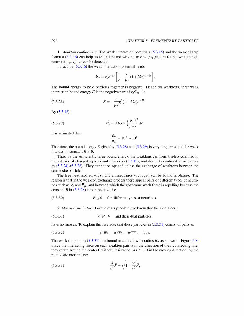
296 CHAPTER 5. ELEMENTARY PARTICLES
1. Weakton confinement. The weak interaction potentials (5.3.15) and the weak charge
formula (5.3.16) can help us to understand why no free w∗,w1,w2 are found, while single
neutrinos νe,νµ ,ντ can be detected.
In fact, by (5.3.15) the weak interaction potential reads
Φw = gse−kr
[1
r− B
ρw
(1+ 2kr)e−kr
],
The bound energy to hold particles together is negative. Hence for weaktons, their weak
interaction bound energy E is the negative part of gsΦw, i.e.
(5.3.28) E =− B
ρw
g2s (1+ 2kr)e−2kr.
By (5.3.16),
(5.3.29) g2w = 0.63×
(ρn
ρw
)6
hc.
It is estimated thatρn
ρw
= 104 ∼ 106.
Therefore, the bound energy E given by (5.3.28) and (5.3.29) is very large provided the weak
interaction constant B > 0.
Thus, by the sufficiently large bound energy, the weaktons can form triplets confined in
the interior of charged leptons and quarks as (5.3.19), and doublets confined in mediators
as (5.3.24)-(5.3.26). They cannot be opened unless the exchange of weaktons between the
composite particles.
The free neutrinos νe,νµ ,ντ and antineutrinos νe,νµ ,ντ can be found in Nature. The
reason is that in the weakton exchange process there appear pairs of different types of neutri-
nos such as νe and νµ , and between which the governing weak force is repelling because the
constant B in (5.3.28) is non-positive, i.e.
(5.3.30) B ≤ 0 for different types of neutrinos.
2. Massless mediators. For the mass problem, we know that the mediators:
(5.3.31) γ, gk, ν and their dual particles,
have no masses. To explain this, we note that these particles in (5.3.31) consist of pairs as
(5.3.32) w1w1, w2w2, w∗w∗, νlν l .
The weakton pairs in (5.3.32) are bound in a circle with radius R0 as shown in Figure 5.8.
Since the interacting force on each weakton pair is in the direction of their connecting line,
they rotate around the center 0 without resistance. As ~F = 0 in the moving direction, by the
relativistic motion law:
(5.3.33)d
dt~P =
√1− v2
c2~F,
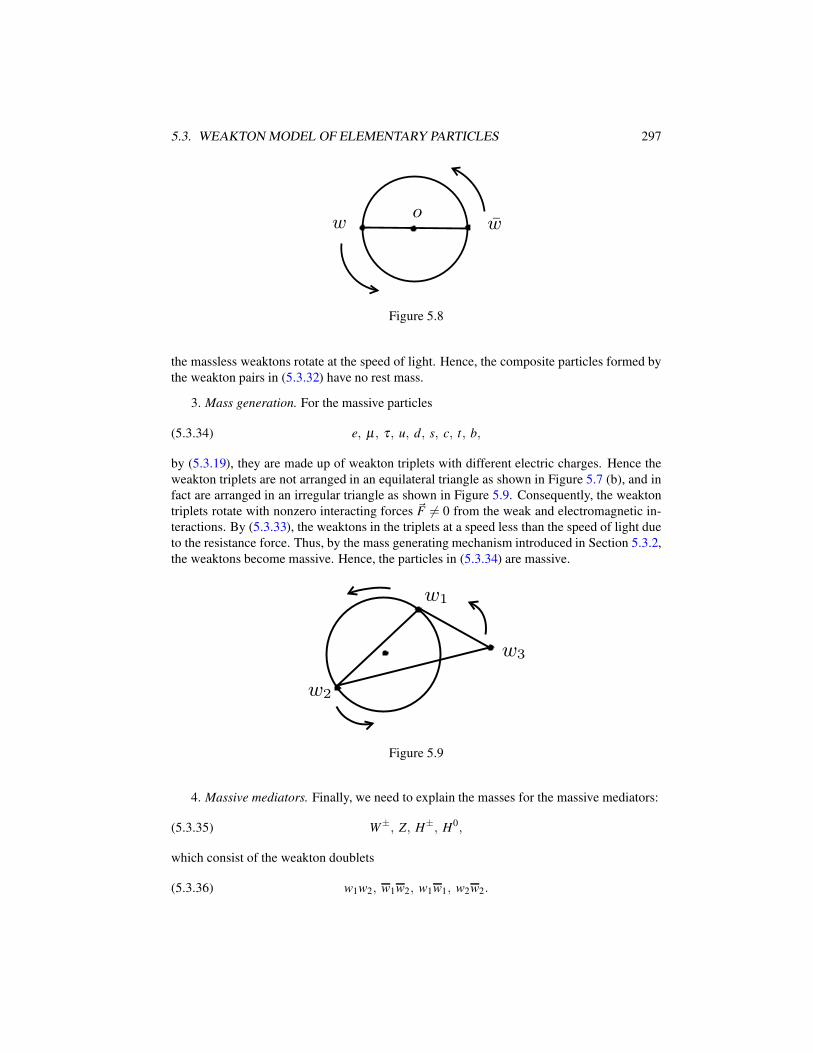
5.3. WEAKTON MODEL OF ELEMENTARY PARTICLES 297
w wo
Figure 5.8
the massless weaktons rotate at the speed of light. Hence, the composite particles formed by
the weakton pairs in (5.3.32) have no rest mass.
3. Mass generation. For the massive particles
(5.3.34) e, µ , τ, u, d, s, c, t, b,
by (5.3.19), they are made up of weakton triplets with different electric charges. Hence the
weakton triplets are not arranged in an equilateral triangle as shown in Figure 5.7 (b), and in
fact are arranged in an irregular triangle as shown in Figure 5.9. Consequently, the weakton
triplets rotate with nonzero interacting forces ~F 6= 0 from the weak and electromagnetic in-
teractions. By (5.3.33), the weaktons in the triplets at a speed less than the speed of light due
to the resistance force. Thus, by the mass generating mechanism introduced in Section 5.3.2,
the weaktons become massive. Hence, the particles in (5.3.34) are massive.
w3
w1
w2
Figure 5.9
4. Massive mediators. Finally, we need to explain the masses for the massive mediators:
(5.3.35) W±, Z, H±, H0,
which consist of the weakton doublets
(5.3.36) w1w2, w1w2, w1w1, w2w2.
298 CHAPTER 5. ELEMENTARY PARTICLES
Actually, in the weakton exchange theory in the next section, we can see that the particles in
(5.3.36) are in some transition states in the weakton exchange procedure. At the moment of
exchange, the weaktons in (5.3.36) are at a speed v with v < c. Hence, the particles in (5.3.35)
are massive, and their life-times are very short (τ ≃ 10−25s).
5.3.6 Quantum rules for weaktons
By carefully examining the quantum numbers of weaktons, the composite particles in (5.3.19)
and (5.3.24)-(5.3.26) are well-defined.
In the last subsection, we solved the free weakton problem and the mass problem. In this
subsection, we propose a few rules to resolve the remainning problems.
1. Weak color neutral rule: All composite particles by weaktons must be weak color
neutral.
Based on this rule, many combinations of weaktons are ruled out. For example, it is clear
that there are no particles corresponding to the following www and ww combinations, because
they all violate the weak color neutral rule:
νew1w2, w∗w2w2, w∗w1w2, etc., νew1, w∗w1, w∗w2 etc.
2. BL = 0,LiL j = 0 (i 6= j), where B is the baryon number, and L = L j = Le,Lµ ,Lτ are
the lepton numbers.
The following combinations of weaktons
w∗νi, νiν j, νiνk (i 6= k),
are not observed in Nature, and are ruled out by this rule.
3. L+Qe = 0, |B+Qe| ≤ 1 for L,B 6= 0.
The following combinations of weaktons
(5.3.37) νiw1w1, νiw2w2, ν iw1w2, w∗w∗ etc
cannot be found in Nature, and are ruled out this rule.
4. Spin selection. In reality, there are no weakton composites with spin J = 32
as
(5.3.38) w∗w1w1(↑↑↑,↓↓↓), w∗w2w2(↑↑↑,↓↓↓), w∗w1w2(↑↑↑,↓↓↓),
and as
(5.3.39) νw1w2 (↑↑↑,↓↓↓).
The cases (5.3.38) are excluded by the Angular Momentum Rule 5.8. The reasons for this
exclusion are two-fold. First, the composite particles in (5.3.38) carry one strong charge, and
consequently, will be confined in a small ball by the strong interaction potential as the quarks
confined in hadrons, as shown in Figure 5.7 (b). Second, due to the uncertainty principle, the
5.3. WEAKTON MODEL OF ELEMENTARY PARTICLES 299
bounding particles will rotate, at high speed with almost zero moment of force, which must
be excluded for composite particles with J 6= 12
based on the angular momentum rule.
The exclusion for (5.3.39) is based on the observation that by the left-hand helicity of
neutrinos with spin J = − 12, one of w1 and w2 must be in the state with J = + 1
2to combine
with ν j (1 ≤ j ≤ 3), i.e. in the manner as
ν jw1w2 (↓,↓↑↓,↑).In summary, under the above rules 1-4, only the weakton constituents in (5.3.19) and
(5.3.24)-(5.3.26) are allowed.
5. Eight quantum states of gluons. It is known that the gluons have eight quantum states
gk : g1, · · · , g8.
In (5.3.24) and (5.3.25), the vector and scalar gluons have the forms
w∗w∗(,) and w∗w∗(↑↓,↓↑).According to QCD, quarks have three colors
red(r), green(g), blue(b),
and anticolor r,g,b. They obey the rules
bb = rr = gg = w ( white).
Based on (5.3.19), w∗ is endowed with three colors and anticolors:
w∗r , w∗
g, w∗b and w∗
r , w∗g, w∗
b,
which form the bases of SU(3) and SU(3). By the irreducible representation:
3× 3 = 8⊕ 1,
we can derive the eight-multiple states as
g1 = (w∗w)w, g2 = w∗bw∗
r , g3 = w∗bw∗
g, g4 = w∗r w∗
g,(5.3.40)
g5 = (w∗w)w, g6 = w∗r w∗
b, g7 = w∗
gw∗b, g8 = w∗
gw∗r .(5.3.41)
where (w∗w∗)w is a linear combination of w∗bw∗
b,w∗
r w∗r ,w
∗gw∗
g. Namely, the gluons in (5.3.41)
are the antigluons of these in (5.3.40).
In summary, the quantum rules presented above can be simply expressed in the following
formulas for quantum numbers Qc,Qe,L and B:
(5.3.42)
weak color neutral: Qc = 0,
mutual exclusion of leptons and baryons: BL = 0, LiL j = 0 (i 6= j),
relation of leptons and charges: L+Qe = 0 (L 6= 0),
relation of baryons and charges: |B+Qe| ≤ 1 (B 6= 0).
These relations are summed up from realistic particle data. Based on (5.3.42), together with
the mass generation mechanism, the Angular Momentum Rule 5.8 and the layered formulas
of weak and strong interaction potentials, all of the most basic problems in the weakton model
have a reasonable explanation.
300 CHAPTER 5. ELEMENTARY PARTICLES
5.4 Mechanisms of Subatomic Decays and Electron Radia-
tions
5.4.1 Weakton exchanges
We conclude that all particle decays are caused by weakton exchange. The exchanges occur
between composite particles as mediators, charged leptons, and quarks.
1. Weakton exchange in mediators. First we consider one of the most important decay
processes in particle physics, the electron-positron pair creation and annihilation:
(5.4.1)2γ → e++ e−,
e++ e− → 2γ.
In fact, the reaction formulas in (5.4.1) are not complete, and the correct formulas should be
as follows
(5.4.2) 2γ +ν e++ e−,
where ν is the ν-mediator as in (5.3.27).
Note that the weakton components of γ and ν are
γ = cosθww1w1 − sinθww2w2,
ν = α1νeνe +α2νµ νµ +α3ντ ντ ,
which imply that the probability of the photon γ at the state w1w1 is cos2 θw and at the state
−w1w2 is sin2 θw, and the probability of ν at νiν i is α2i . Namely, for photon, the densities of
the w1w1() and −w2w2() particle states are cos2 θw and sin2 θw, and the densities of the
states νeνe,νµ νµ , ντ ντ are α21 ,α
22 ,α
23 . Hence the formula (5.4.2) can be written as
(5.4.3) w1w1()+w2w2()+νeνe(↓↑) νew1w2(↓↑↓)+νew1w2(↓).
It is then clear to see from (5.4.3) that the weakton constituents w1,w1,w2,w2,νe,νe can
regroup due to the weak interaction, and we call this process weakton exchange. The mech-
anism of this exchanging process can be explained using the layered formulas in (5.3.15) of
weak interaction potentials.
The layered potential formulas in (5.3.15) indicate that each composite particle has an
exchange radius R, which satisfies
(5.4.4) ρ < R < ρ1,
where ρ is the radius of this particle and ρ1 is its repelling radius of weak force. If two
composite particles A and B are in a distance less than their common exchange radius, then
the weaktons in A and B are attracting to each other by their weak interacting forces generated
by Φw0 in (5.3.15), given by
(5.4.5) Φw0 = gwe−kr
[1
r− Bw
ρw
(1+ 2kr)e−kr
].
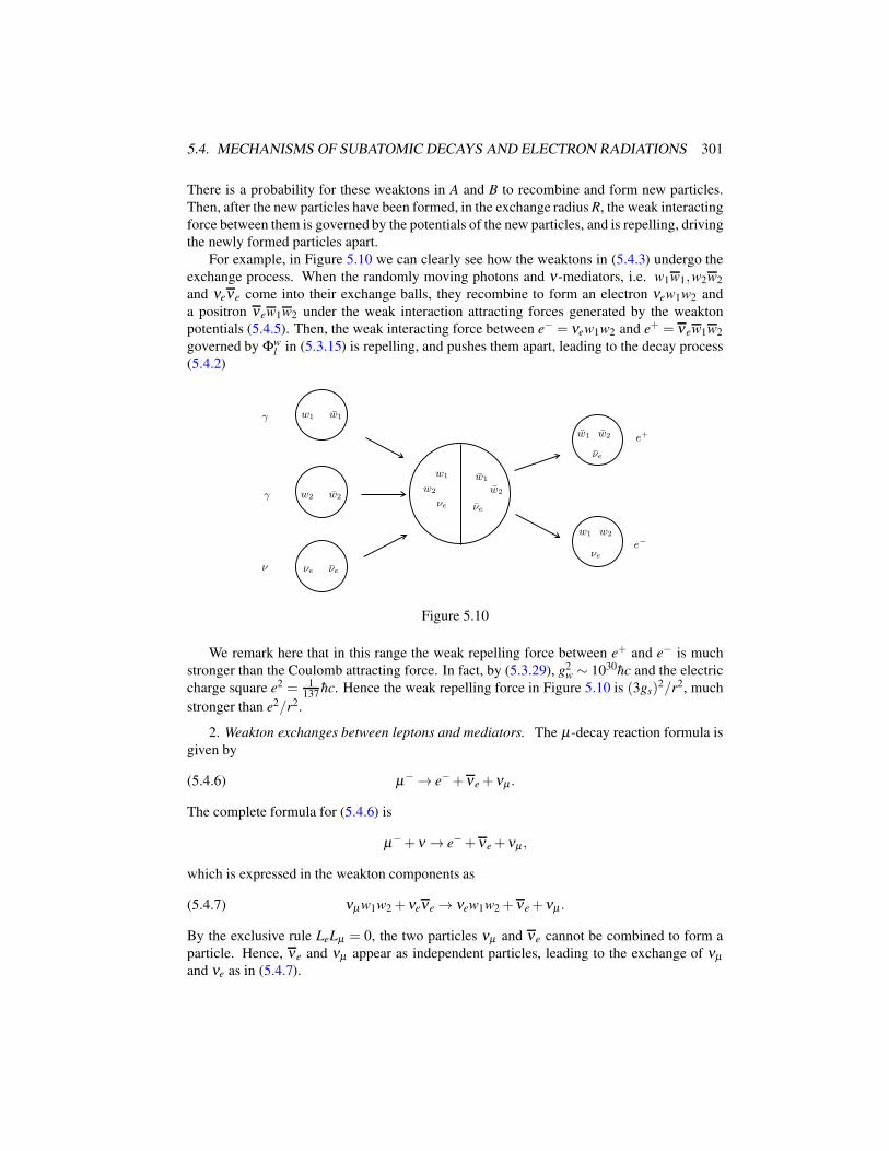
5.4. MECHANISMS OF SUBATOMIC DECAYS AND ELECTRON RADIATIONS 301
There is a probability for these weaktons in A and B to recombine and form new particles.
Then, after the new particles have been formed, in the exchange radius R, the weak interacting
force between them is governed by the potentials of the new particles, and is repelling, driving
the newly formed particles apart.
For example, in Figure 5.10 we can clearly see how the weaktons in (5.4.3) undergo the
exchange process. When the randomly moving photons and ν-mediators, i.e. w1w1,w2w2
and νeνe come into their exchange balls, they recombine to form an electron νew1w2 and
a positron νew1w2 under the weak interaction attracting forces generated by the weakton
potentials (5.4.5). Then, the weak interacting force between e− = νew1w2 and e+ = νew1w2
governed by Φwl in (5.3.15) is repelling, and pushes them apart, leading to the decay process
(5.4.2)
w1 w1
w2 w2
νe νe
w1 w1
w2
νe
w1 w2
νe
νe
w1 w2
γ
γ
ν
w2
νe
e+
e−
Figure 5.10
We remark here that in this range the weak repelling force between e+ and e− is much
stronger than the Coulomb attracting force. In fact, by (5.3.29), g2w ∼ 1030hc and the electric
charge square e2 = 1137
hc. Hence the weak repelling force in Figure 5.10 is (3gs)2/r2, much
stronger than e2/r2.
2. Weakton exchanges between leptons and mediators. The µ-decay reaction formula is
given by
(5.4.6) µ− → e−+νe +νµ .
The complete formula for (5.4.6) is
µ−+ν → e−+νe +νµ ,
which is expressed in the weakton components as
(5.4.7) νµw1w2 +νeνe → νew1w2 +νe +νµ .
By the exclusive rule LeLµ = 0, the two particles νµ and νe cannot be combined to form a
particle. Hence, νe and νµ appear as independent particles, leading to the exchange of νµ
and νe as in (5.4.7).
302 CHAPTER 5. ELEMENTARY PARTICLES
3. Weakton exchanges between quarks and mediators. The d-quark decay in (5.3.2) is
written as
(5.4.8) d → u+ e−+νe.
The correct formula for (5.4.8) is
d+ γ +ν → u+ e−+νe,
which, in the weakton components, is given by
(5.4.9) w∗w1w2 +w1w1 +νeνe → w∗w1w1 +νew1w2 +νe.
In (5.4.9), the weakton pair w2 and w1 is exchanged, and νe is captured by the new doublet
w1w2, which is the vector boson W−, to form an electron νew1w2.
5.4.2 Conservation laws
The weakton exchanges must obey certain conservation laws, which are listed in the follow-
ing.
1. Conservation of weakton numbers. The weaktons given in (5.3.18) are elementary
particles, which cannot undergo any decay. Also, the w-weaktons cannot be converted be-
tween each other. Although the neutrino oscillation, which is unconfirmed, may convert one
flavour of neutrino to another, for a particle decay or scattering, the neutrino number is still
conserved. Namely, the lepton numbers Le,Lµ ,Lτ are conserved.
Therefore, for any particle reaction:
(5.4.10) A1 + · · ·+AN → B1 + · · ·+BK,
the number of each weakton type is invariant. Namely, for any type of weakton w, its number
is conserved in (5.4.10):
NAw = NB
w ,
where NAw
and NBw
are the numbers of the w weaktons in both sides of (5.4.10).
2. Spin conservation. The spin of each weakton is invariant. The conservation of weakton
number implies that the spin is also conserved:
JA1+ · · ·+ JAN
= JB1+ · · ·+ JBK
,
where JA is the spin of particle A.
In classical particle theories, the spin is not considered as a conserved quantity. The
reason for the non-conservation of spin is due to the incompleteness of the reaction formulas
given in Section 5.1.3. Hence, spin conservation can also be considered as an evidence for
the incompleteness of those reaction formulas. The incomplete decay reaction formulas can
be made complete by supplementing some massless mediators, so that the spin becomes a
conserved quantum number.
5.4. MECHANISMS OF SUBATOMIC DECAYS AND ELECTRON RADIATIONS 303
3. Energy conservation. Energy conservation is a universal physical law for all particle
systems. Hence, the energy conservation has also to be satisfied by the weakton exchanges.
This law is manifested in the following prohibitions for decays:
(5.4.11)
e− 9 µ−+νµ +νe,
e− 9 τ−+ντ +νe,
µ−9 τ−+ντ +νµ .
The complete reaction formulas for (5.4.11) are
(5.4.12)
νew1w2 +νµνµ → νµ w1w2 +νµ +νe,
νew1w2 +ντ ντ → ντ w1w2 +ντ +νe,
νµw1w2 +ντ ντ → ντ w1w2 +ντ +νµ .
From the viewpoints of quantum rules given by (5.3.42) and weakton number conservation,
the decays in (5.4.12) are allowed. However, due to the mass relations
me < mµ < mτ ,
these weakton exchange processes (5.4.12) violate the energy conservation. Therefore these
decays cannot occur. However, if ν-mediators have high energy to hit electrons, then the
reactions (5.4.12) may occur.
In a weakton exchange process, the energy conservation law can be explicitly expressed
as follows:
Energy Rule 5.13. The composite particles with the lower masses cannot undergo weakton
exchanges with massless mediators in lower energy to decay into the composite particles with
higher masses.
We remark that the Energy Rule 5.13 is sharper than the energy conservation law. In
fact, the reaction formulas from lower masses to higher masses do not imply that the energy
conservation must be violated. Hence, it is possible that there exist more basic unknown
physical laws under the Energy Rule 5.13.
4. Other conservative quantum numbers. From the invariance of weakton numbers, we
deduce immediately the following conserved quantum numbers:
electric charge Qe, weak charge Qw, strong charge Qs,
baryon number B, lepton numbers Le, Lµ , Lτ .
5.4.3 Decay types
In particle physics, the reactions listed in Section 5.1.3 are classified into two types: the weak
interacting type and the strong interacting type. However, there are no clear definitions to
distinguish them. Usual methods are by experiments to determine reacting intensity, i.e. the
transition probability. In general, the classification is derived based on
weak type: i) presence of leptons in the reactions,
ii) change of strange numbers,
strong type: otherwise.
304 CHAPTER 5. ELEMENTARY PARTICLES
With the weakton model, all decays are carried out by exchanging weaktons. Hence decay
types can be fully classified into three types: the weak type, the strong type, and the mixed
type, based on the type of forces acting on the final particles after the weakton exchange
process.
For example, the reactions
(5.4.13)
νµ + e− → µ−+νe,
n → p+ e−+νe,
π0 → γ + γ.
are weak decays,
(5.4.14) ∆++ → p++π+
is a strong decay, and
(5.4.15) Λ → p++π− ( i.e. Λ+ gk + 3γ → p++π−+ γ)
is a mixed decay.
In view of (5.4.13)-(5.4.15), the final particles contain at most one hadron in a weak decay,
contain no leptons and no mediators in a strong decay, and contain at least two hadrons and a
lepton or a mediator in a mixed decay.
In summary, we give the criteria for decay types based on the particles appearing in the
final step of the decay process:
(5.4.16)
weak decay: at most one hadron,
strong decay: no leptons and no mediators,
mixed decay: others.
Remark 5.14. The new classification is easy to understand, and the criterion (5.4.16) pro-
vides a convenient method for us to distinguish the different types of decays and scatterings.
In fact, this classification truly reflects the roles of interactions in particle reaction processes.
5.4.4 Decays and scatterings
Decays and non-elastic scatterings are caused by weakton exchanges. The massless mediators
(5.4.17) γ, gk, γ0, gk0, ν,
spread over the space or around the charged leptons and quarks at various energy levels, and
most of them are at low energy states. It is these random mediators in (5.4.17) entering the
exchange radius of matter particles that generate decays. In the following we shall discuss
these reaction processes for various types of decays and scatterings.
Weak types
1. First we consider the e-µ scattering
νµ + e− → µ−+νe,
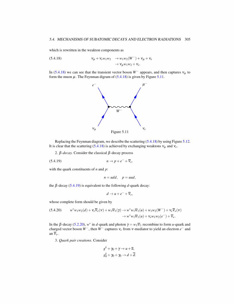
5.4. MECHANISMS OF SUBATOMIC DECAYS AND ELECTRON RADIATIONS 305
which is rewritten in the weakton components as
νµ +νew1w2 → w1w2(W−)+νµ +νe(5.4.18)
→ νµ w1w2 +νe.
In (5.4.18) we can see that the transient vector boson W− appears, and then captures νµ to
form the muon µ . The Feynman digram of (5.4.18) is given by Figure 5.11.
W−
νµ
e−
νe
µ−
Figure 5.11
Replacing the Feynman diagram, we describe the scattering (5.4.18) by using Figure 5.12.
It is clear that the scattering (5.4.18) is achieved by exchanging weaktons νµ and νe.
2. β -decay. Consider the classical β -decay process
(5.4.19) n → p+ e−+νe.
with the quark constituents of n and p:
n = udd, p = uud,
the β -decay (5.4.19) is equivalent to the following d-quark decay:
d → u+ e−+νe,
whose complete form should be given by
w∗w1w2(d)+νeνe(ν)+w1w1(γ)→ w∗w1w1(u)+w1w2(W−)+νeνe(ν)(5.4.20)
→ w∗w1w1(u)+νew1w2(e−)+νe.
In the β -decay (5.2.20), w∗ in d-quark and photon γ = w1w1 recombine to form u-quark and
charged vector boson W−, then W− captures νe from ν-mediator to yield an electron e− and
an νe.
3. Quark pair creations. Consider
gk + γ0 + γ → u+ u,
gk0 + γ0 + γ0 → d + d.
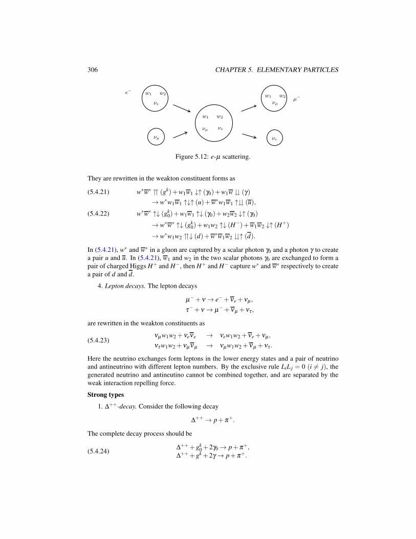
306 CHAPTER 5. ELEMENTARY PARTICLES
w1 w2
νµ
w1 w2
νe
w1 w2
νe
νe
νµ
νµ
e−
µ−
Figure 5.12: e-µ scattering.
They are rewritten in the weakton constituent forms as
w∗w∗ (gk)+w1w1 ↓↑ (γ0)+w1w (γ)(5.4.21)
→ w∗w1w1 ↑↓↑ (u)+w∗w1w1 ↑ (u),
w∗w∗ ↑↓ (gk0)+w1w1 ↑↓ (γ0)+w2w2 ↓↑ (γ0)(5.4.22)
→ w∗w∗ ↑↓ (gk0)+w1w2 ↑↓ (H−)+w1w2 ↓↑ (H+)
→ w∗w1w2 ↓ (d)+w∗w1w2 ↑ (d).
In (5.4.21), w∗ and w∗ in a gluon are captured by a scalar photon γ0 and a photon γ to create
a pair u and u. In (5.4.21), w1 and w2 in the two scalar photons γ0 are exchanged to form a
pair of charged Higgs H+ and H−, then H+ and H− capture w∗ and w∗ respectively to create
a pair of d and d.
4. Lepton decays. The lepton decays
µ−+ν → e−+νe +νµ ,
τ−+ν → µ−+νµ +ντ ,
are rewritten in the weakton constituents as
(5.4.23)νµ w1w2 +νeνe → νew1w2 +νe +νµ ,
ντ w1w2 +νµνµ → νµw1w2 +νµ +ντ .
Here the neutrino exchanges form leptons in the lower energy states and a pair of neutrino
and antineutrino with different lepton numbers. By the exclusive rule LiL j = 0 (i 6= j), the
generated neutrino and antineutino cannot be combined together, and are separated by the
weak interaction repelling force.
Strong types
1. ∆++-decay. Consider the following decay
∆++ → p+π+.
The complete decay process should be
(5.4.24)∆+++ gk
0 + 2γ0 → p+π+,∆+++ gk + 2γ → p+π+.
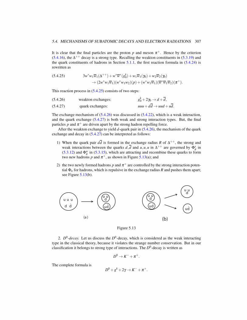
5.4. MECHANISMS OF SUBATOMIC DECAYS AND ELECTRON RADIATIONS 307
It is clear that the final particles are the proton p and meson π+. Hence by the criterion
(5.4.16), the ∆++ decay is a strong type. Recalling the weakton constituents in (5.3.19) and
the quark constituents of hadrons in Section 5.1.1, the first reaction formula in (5.4.24) is
rewritten as
3w∗w1w1(∆++)+w∗w∗(gk
0)+w1w1(γ0)+w2w2(γ0)(5.4.25)
→ (2w∗w1w1)(w∗w1w2)(p)+ (w∗w1w1)(w
∗w1w2)(π+).
This reaction process in (5.4.25) consists of two steps:
weakton exchanges: gk0 + 2γ0 → d+ d,(5.4.26)
quark exchanges: uuu+ dd → uud+ ud.(5.4.27)
The exchange mechanism of (5.4.26) was discussed in (5.4.22), which is a weak interaction,
and the quark exchange (5.4.27) is both weak and strong interaction types. But, the final
particles p and π+ are driven apart by the strong hadron repelling force.
After the weakton exchange to yield d-quark pair in (5.4.26), the mechanism of the quark
exchange and decay in (5.4.27) can be interpreted as follows:
1) When the quark pair dd is formed in the exchange radius R of ∆++, the strong and
weak interactions between the quarks d,d and u,u,u in ∆++ are governed by Φsq in
(5.3.12) and Φwq in (5.3.15), which are attracting and recombine these quarks to form
two new hadrons p and π+, as shown in Figure 5.13(a); and
2) the two newly formed hadrons p and π+ are controlled by the strong interaction poten-
tial Φn for hadrons, which is repulsive in the exchange radius R and pushes them apart;
see Figure 5.13(b).
u u u
d d
u u
ud
d
(a )
u u
ud
d
u u
ud
d
(b)
Figure 5.13
2. D0-decay. Let us discuss the D0-decay, which is considered as the weak interacting
type in the classical theory, because it violates the strange number conservation. But in our
classification it belongs to strong type of interactions. The D0-decay is written as
D0 → K−+π+.
The complete formula is
D0 + gk + 2γ → K−+π+.
308 CHAPTER 5. ELEMENTARY PARTICLES
The weakton constituents of this decay is given by
(w∗w2w2)(w∗w1w1)(cu)+w∗w∗(gk)+ 2w1w1(γ)
→ (w∗w1w2)(w∗w1w1)(cu)+ (w∗w1w1)(w
∗w1w2)(ud).
This reaction is due to the c-quark decay
c+ gk + 2γ → s+ u+ d,
which is given in the weakton constituents as
w∗w2w2(c)+w∗w∗(gk)+ 2w1w1(γ)→ w∗w1w2(s)+w∗w1w1(u)+w∗w1w2(d).(5.4.28)
The reaction (5.4.28) consists of two exchange processes:
(5.4.29) w∗w2w2(c)+w1w1(γ)→ w∗w1w2(s)+w1w2(w−),
and
(5.4.30) w1w2(W−)+w1w1(γ)+ (w∗w∗)(gk)→ w∗w1w1(u)+w∗w1w2(d)
It is clear that both exchanges (5.4.29) and (5.4.30) belong to weak interactions. However,
the final particles in the D0-decay are K− and π+, which are separated by the strong hadron
repelling force. The principle for the quark exchange and hadron separation in the D0-decay
process is the same as shown in Figure 5.13.
Remark 5.15. In the mechanism of subatomic particle decays and scatterings, the layered
properties of the weak and strong interacting forces play a crucial role. Namely the attract-
ing and repelling radii of weak and strong forces for a particle depend on its radius ρ and
interaction constants A and B or equivalently the parameters
(5.4.31)A
ρin (5.3.11) and
B
ρin (5.3.14).
These parameters determine the attracting and repelling regions of the particle. Hence, in the
exchange radius of particles, the weak and strong forces are attracting between weaktons and
quarks, and are repelling between the final particles in decays and scatterings. The reason is
that the parameters in (5.4.31) are different at various levels of subatomic particles.
Mixed decays
The typical mixed decay is the Λ-decay, written as
Λ → p+π−.
The correct form of Λ-decay should be
(5.4.32) Λ+ gk + 2γ + γ0 → p+π−+ γ0.
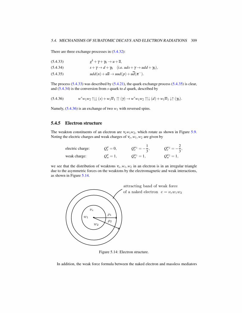
5.4. MECHANISMS OF SUBATOMIC DECAYS AND ELECTRON RADIATIONS 309
There are three exchange processes in (5.4.32):
gk + γ + γ0 → u+ u,(5.4.33)
s+ γ → d+ γ0 (i.e. uds+ γ → udd+ γ0),(5.4.34)
udd(n)+ uu→ uud(p)+ ud(π−).(5.4.35)
The process (5.4.33) was described by (5.4.21), the quark exchange process (5.4.35) is clear,
and (5.4.34) is the conversion from s quark to d quark, described by
(5.4.36) w∗w1w2 ↑ (s)+w1w1 (γ)→ w∗w1w2 ↓ (d)+w1w1 ↓↑ (γ0).
Namely, (5.4.36) is an exchange of two w1 with reversed spins.
5.4.5 Electron structure
The weakton constituents of an electron are νew1w2, which rotate as shown in Figure 5.9.
Noting the electric charges and weak charges of νe,w1,w2 are given by
electric charge: Qνe = 0, Qw1
e =−1
3, Qw2
e =−2
3,
weak charge: Qνw = 1, Qw1
w = 1, Qw2w = 1,
we see that the distribution of weaktons νe,w1,w2 in an electron is in an irregular triangle
due to the asymmetric forces on the weaktons by the electromagnetic and weak interactions,
as shown in Figure 5.14.
ρ1
ρ2
νe
w1
w2
attracting band of weak force
of a naked electron e = νew1w2
Figure 5.14: Electron structure.
In addition, the weak force formula between the naked electron and massless mediators
310 CHAPTER 5. ELEMENTARY PARTICLES
γ,γ0,gk,gk
0,ν , is given by
Fw =− gw(ρm)gw(ρe)∂
∂ r
[1
re−kr − B
ρ(1+ 2kr)e−2kr
],(5.4.37)
=gw(ρm)gw(ρe)e−kr
[1
r2+
1
rr0
− 4B
ρ
r
r20
e−kr
],
where k = 1/r0 = 1016 cm−1,gw(ρm) and gw(ρe) are the weak charges of mediators and the
naked electron, expressed as
gw(ρm) = 2
(ρw
ρm
)3
gw, gw(ρe) = 3
(ρw
ρe
)3
gw,
and B/ρ is a parameter determined by the naked electron and mediators.
By the weak force formula (5.4.37), there is an attracting shell region of weak interaction
between naked electron and mediators
(5.4.38) ρ1 < r < ρ2
as shown in Figure 5.13, with small weak force, where ρ j ( j = 1,2) are the zero points of
(5.4.37). Namely, they satisfy that
e−kρ j ρ3j =
ρ
4B
(1+
ρ j
r0
)for 1 ≤ j ≤ 2.
In the region (5.4.38), the weak force is attracting, and outside this region the weak force is
repelling:
(5.4.39) Fw
< 0 for ρ1 < r < ρ2,
> 0 for r < ρ1 and ρ2 < r.
Since the mediators γ,γ0,gk,gk
0 and ν contain two weak charges Qw = 2gw, by (5.4.39)
they are attached to the electron in the attracting shell region (5.4.38), forming a cloud of
mediators. The irregular triangle distribution of the weaktons νe,w1,w2 generate a small
moment of force on the mediators. Meanwhile there also exist weak forces between them.
Therefore the bosons will rotate at a speed less than the speed of light, and generate a small
mass attached to the naked electron νew1w2.
5.4.6 Mechanism of bremsstrahlung
It is known that an electron emits photons as its velocity changes, which is called the bremsstrahlung.
The reasons why bremsstrahlung can occur is unknown in classical theories. Based on the
electron structure theory established in the last subsection, we present here a mechanism of
this phenomenon.
In fact, if an electron is situated in an electromagnetic field, then the electromagnetic
field exerts a Coulomb force on ithe naked electron νew1w2, but not on the attached neutral
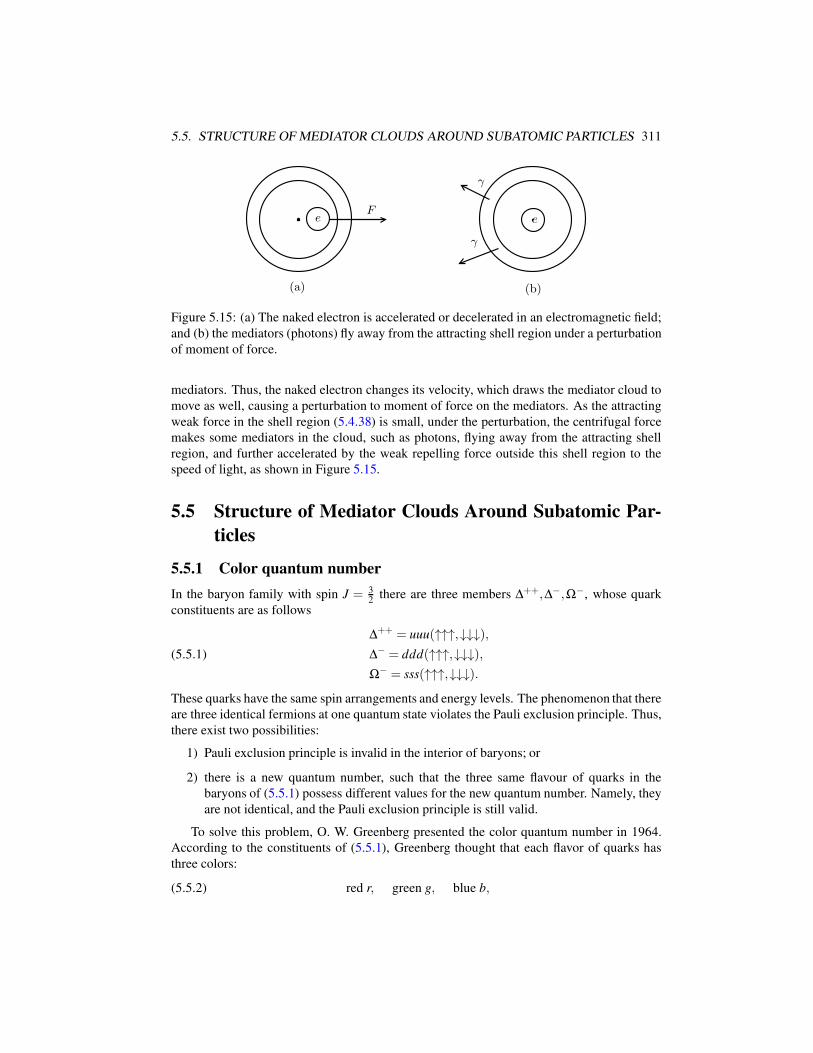
5.5. STRUCTURE OF MEDIATOR CLOUDS AROUND SUBATOMIC PARTICLES 311
eF
(a)
e
γ
(b)
γ
Figure 5.15: (a) The naked electron is accelerated or decelerated in an electromagnetic field;
and (b) the mediators (photons) fly away from the attracting shell region under a perturbation
of moment of force.
mediators. Thus, the naked electron changes its velocity, which draws the mediator cloud to
move as well, causing a perturbation to moment of force on the mediators. As the attracting
weak force in the shell region (5.4.38) is small, under the perturbation, the centrifugal force
makes some mediators in the cloud, such as photons, flying away from the attracting shell
region, and further accelerated by the weak repelling force outside this shell region to the
speed of light, as shown in Figure 5.15.
5.5 Structure of Mediator Clouds Around Subatomic Par-
ticles
5.5.1 Color quantum number
In the baryon family with spin J = 32
there are three members ∆++,∆−,Ω−, whose quark
constituents are as follows
∆++ = uuu(↑↑↑,↓↓↓),∆− = ddd(↑↑↑,↓↓↓),(5.5.1)
Ω− = sss(↑↑↑,↓↓↓).These quarks have the same spin arrangements and energy levels. The phenomenon that there
are three identical fermions at one quantum state violates the Pauli exclusion principle. Thus,
there exist two possibilities:
1) Pauli exclusion principle is invalid in the interior of baryons; or
2) there is a new quantum number, such that the three same flavour of quarks in the
baryons of (5.5.1) possess different values for the new quantum number. Namely, they
are not identical, and the Pauli exclusion principle is still valid.
To solve this problem, O. W. Greenberg presented the color quantum number in 1964.
According to the constituents of (5.5.1), Greenberg thought that each flavor of quarks has
three colors:
(5.5.2) red r, green g, blue b,
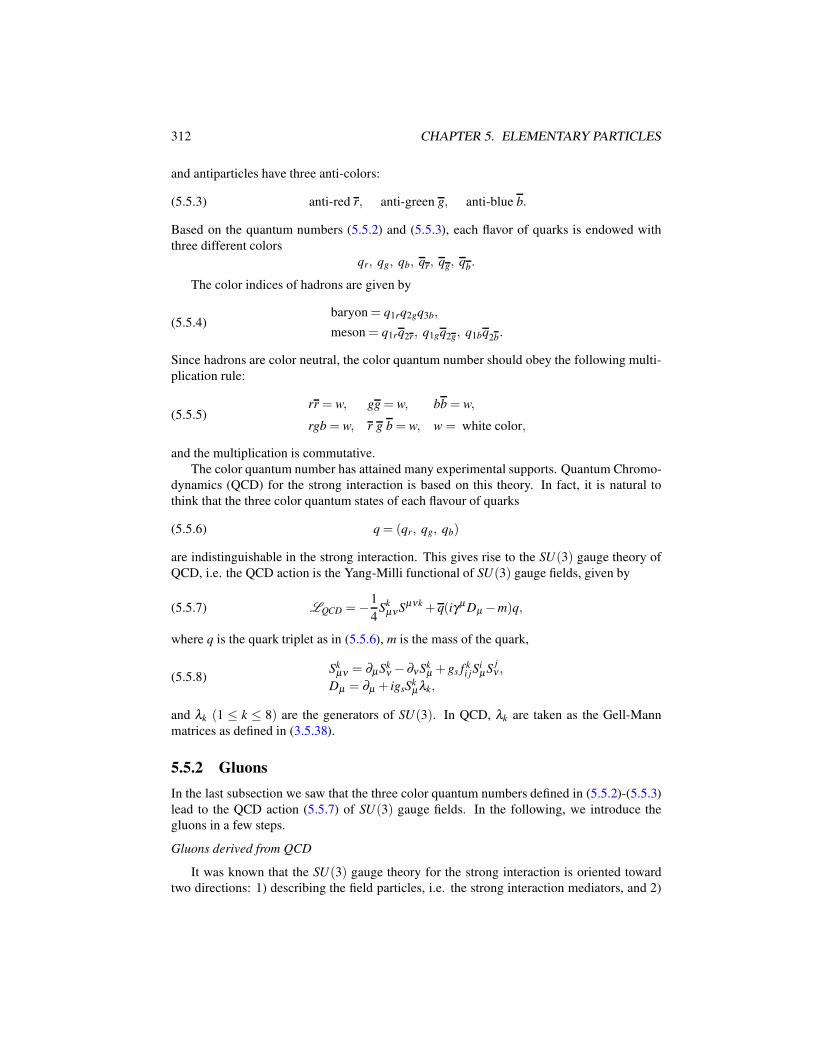
312 CHAPTER 5. ELEMENTARY PARTICLES
and antiparticles have three anti-colors:
(5.5.3) anti-red r, anti-green g, anti-blue b.
Based on the quantum numbers (5.5.2) and (5.5.3), each flavor of quarks is endowed with
three different colors
qr, qg, qb, qr, qg, qb.
The color indices of hadrons are given by
(5.5.4)baryon = q1rq2gq3b,
meson = q1rq2r, q1gq2g, q1bq2b.
Since hadrons are color neutral, the color quantum number should obey the following multi-
plication rule:
(5.5.5)rr = w, gg = w, bb = w,
rgb = w, r g b = w, w = white color,
and the multiplication is commutative.
The color quantum number has attained many experimental supports. Quantum Chromo-
dynamics (QCD) for the strong interaction is based on this theory. In fact, it is natural to
think that the three color quantum states of each flavour of quarks
(5.5.6) q = (qr, qg, qb)
are indistinguishable in the strong interaction. This gives rise to the SU(3) gauge theory of
QCD, i.e. the QCD action is the Yang-Milli functional of SU(3) gauge fields, given by
(5.5.7) LQCD =−1
4Sk
µνSµνk + q(iγµ Dµ −m)q,
where q is the quark triplet as in (5.5.6), m is the mass of the quark,
(5.5.8)Sk
µν = ∂µSkν − ∂νSk
µ + gs f ki jS
iµS
jν ,
Dµ = ∂µ + igsSkµλk,
and λk (1 ≤ k ≤ 8) are the generators of SU(3). In QCD, λk are taken as the Gell-Mann
matrices as defined in (3.5.38).
5.5.2 Gluons
In the last subsection we saw that the three color quantum numbers defined in (5.5.2)-(5.5.3)
lead to the QCD action (5.5.7) of SU(3) gauge fields. In the following, we introduce the
gluons in a few steps.
Gluons derived from QCD
It was known that the SU(3) gauge theory for the strong interaction is oriented toward
two directions: 1) describing the field particles, i.e. the strong interaction mediators, and 2)
5.5. STRUCTURE OF MEDIATOR CLOUDS AROUND SUBATOMIC PARTICLES 313
providing strong interaction potentials. In Section 4.5, we have discussed problem 2). Here,
we consider problem 1).
Experiments showed that there are eight field particles for the strong interaction, called
gluons, which are massless and electric neutral, denoted by
(5.5.9) gk, 1 ≤ k ≤ 8.
The QCD theory shows that the gluons are vector bosons with spin J = 1.
Based on both the unified field theory and the weakton model, corresponding to the vector
gluons (5.5.9) there are eight dual field particles, which are scalar bosons with spin J = 0,
denoted by
(5.5.10) gk0, 1 ≤ k ≤ 8.
In addition, by PID, it follows from (5.5.7)-(5.5.8) that the field equations describing the
eight vector gluons (5.5.9) read
∂ νSkµν −
gs
hcf ki jg
αβ SiαµS
j
β− gsQ
kµ = (∂µ +
gs
hcαlS
lµ −
1
4α0xµ)φ
ks ,(5.5.11)
for 1 ≤ k ≤ 8, and the field equations describing the eight scalar gluons (5.5.10) are
∂ µ ∂µφ ks + ∂ µ
[(gs
hcαlS
lµ −
1
4α0xµ
)φ k
s
]=−gs∂
µQkµ − gs
hcf ki jg
αβ ∂ µ(SiαµS
j
β ),(5.5.12)
for 1 ≤ k ≤ 8, where αl (1 ≤ l ≤ 8) and α0 are parameters, and
Qkµ = qγµ λ kq (λ k = λk, γµ = gµνγν).
The field equations (5.5.11) and (5.5.12) are as in (4.4.34) and (4.4.37).
From (5.5.11) and (5.5.12) we can deduce the following theoretical conclusions for the
gluons (5.5.9) and dual gluons (5.5.10):
1) The field functions W kµ (1 ≤ k ≤ 8) describing the gluons (5.5.9) are vector fields, and,
therefore, gk in (5.5.9) are vector bosons with spin J = 1;
2) The field function φ ks (1 ≤ k ≤ 8) describing the gluons (5.5.10) are scalar fields, and
therefore gk0 in (5.5.10) are scalar bosons with J = 0;
3) The field equations (5.5.11) and (5.5.12) are nonlinear. Consequently, the gluons gk
and gk0 are not in free states, and in their bound states the masses of gk and gk
0 may
appear;
4) In the bound states, the masses can be generated by the spontaneous symmetry breaking
in (5.5.11) and (5.5.12), and the mass terms for gk and gk0 are as follows
gk :gs
hcαl φ
ks Sl
µ (φ kl are the ground states),
gk0 : α0Φk
s ;
314 CHAPTER 5. ELEMENTARY PARTICLES
5) Free gluons, if there exist, are massless.
Remark 5.16. Gluons and photons are massless only in their free states. When they are
confined in mediator clouds around electrons and quarks, they may attain masses. In this
case, massive photons are described by the PID electromagnetic equations as follows:
Vector photons:
(5.5.13) ∂ ν (∂νAµ − ∂µAν)− eJµ = (∂µ +e
hcβ Aµ −
1
4kxµ)φ .
Scalar photons:
(5.5.14) ∂ µ ∂µφ − kφ +e
hcβ ∂ µ(Aµφ)− 1
4kxµ∂ µ φ = 0.
The masses of bound photons are created in (5.5.13) and (5.5.14) by the spontaneous gauge-
symmetry breaking.
Color charge
In the QCD theory, color quantum numbers are regarded as color charges. Namely, each
quark carries one of the color charges:
(5.5.15)red charge r, green charge g, blue charge b,
anti-red charge r, anti-green charge g, anti-blue charge b.
Each gluon is considered to carry a pair of a color charge and an anti-color charge in QCD.
Thus, the three pair of color charges and anti-color charges in (5.5.15) constitute fundamental
bases of SU(3) and SU(3), and the gluons gk (1 ≤ k ≤ 8) form an octet of the irreducible
representation
SU(3)⊗ SU(3) = 8⊕ 1,
which are expressed as
g1 = rg, g2 = br, g3 = gb, g4 =1√2(rr− bb),(5.5.16)
g5 = gr, g6 = rb, g7 = bg, g8 = g4.(5.5.17)
We remark that the conclusions (5.5.16) and (5.5.17) of QCD for gluons are completely
consistent with those in the weakton model in (5.3.40) and (5.3.41). However, the QCD
version is based on the color charges of (5.5.15), and the version of weakton model is based
on the color quantum number of the w∗-weakton:
w∗r , w∗
g, w∗b, w∗
r , w∗g, w∗
b.
Gluon radiation
Based on the Standard Model, quarks can emit and absorb gluons in the same fashion as
electrons emitting and absorbing photons. For example, a red u-quark ur emits an rg gluon
grg, then ur becomes a ug quark, as shown in Figure 5.16.
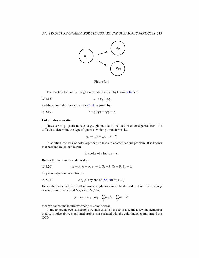
5.5. STRUCTURE OF MEDIATOR CLOUDS AROUND SUBATOMIC PARTICLES 315
ur
ug
urg
Figure 5.16
The reaction formula of the gluon radiation shown by Figure 5.16 is as
(5.5.18) ur → ug + grg,
and the color index operation for (5.5.18) is given by
(5.5.19) r = g(rg) = rgg = r.
Color index operation
However, if qr-quark radiates a gbq gluon, due to the lack of color algebra, then it is
difficult to determine the type of quark to which qr transforms, i.e.
qr → gbg + qX , X =?.
In addition, the lack of color algebra also leads to another serious problem. It is known
that hadrons are color neutral:
the color of a hadron = w.
But for the color index ci defined as
(5.5.20) c1 = r, c2 = g, c3 = b, c1 = r, c2 = g, c3 = b,
they is no algebraic operation, i.e.
(5.5.21) cic j 6= any one of (5.5.20) for i 6= j.
Hence the color indices of all non-neutral gluons cannot be defined. Thus, if a proton p
contains three quarks and N gluons (N 6= 0):
p = uci+ uc j
+ dck+∑
k
nkgk, ∑k
nk = N,
then we cannot make sure whether p is color neutral.
In the following two subsections we shall establish the color algebra, a new mathematical
theory, to solve above mentioned problems associated with the color index operation and the
QCD.
316 CHAPTER 5. ELEMENTARY PARTICLES
5.5.3 Color algebra
The main objective of this and next subsections is to introduce a consistent color algebraic
structure, and to establish a color index formula for hadrons and color transformation ex-
change for gluon radiation.
The color algebra for quantum chromodynamics (QCD) established here is based on color
neutral principle of hadrons, and is uniquely determined. Hence it serves as the mathematical
foundation of QCD.
Color algebra of color quantum numbers
First we examine the crucial problems encountered in the existing theory for color al-
gebra. The color neutral principle of hadrons requires that the three colors must obey the
following laws:
rgb = w, r g b = w,(5.5.22)
rr = gg = bb = w.(5.5.23)
Basic physical considerations imply that the product operation of color indices is com-
mutative and associative:
rg = gr, rb = br, bg = gb, rgb = (rg)b = r(gb).
Hence we infer from (5.5.22) and (5.5.23) that
(5.5.24)rg = b, rb = g, bg = r,r g = b, rb = g, bg = r.
Notice that the white color w is the unit element, i.e.
wr = r, wg = g, wb = b, wr = r, wg = g, wb = b.
Then again, we infer from (5.5.22) and (5.5.23) that
(5.5.25)rr = r, gg = g, bb = b,
r r = r, g g = g, b b = b.
Multiplying (5.5.22) by b and using (5.5.25), we deduce that
(5.5.26) r(gb) = b,
which leads to inconsistency, no matter what color we assign for gb. For example, if we
assign gb = r, then we derive from (5.5.26) that rr = b, which is inconsistent with rr = r in
(5.4.25). If we assume gb = b, then rb = b, which, by multiplying by b, leads to r = bb = b,
a contradiction again.
The above inconsistency demonstrates that in addition to the six basic color indices
r, g, b, r, g, b,
we need to incorporate the following color extensions:
rg, rg, rb, rb, gb, gb.
5.5. STRUCTURE OF MEDIATOR CLOUDS AROUND SUBATOMIC PARTICLES 317
Only two of these added color indices are independent, and in fact, we can derive from
(5.5.24) that
rg = br = gb, gr = rb = bg.
Hence we define them as yellow y and anti-yellow y as follows:
(5.5.27)y = rg = br = gb,y = gr = rb = bg.
In a nutshell, in order to establish a consistent color algebra, it is necessary to add two quan-
tum numbers yellow y and anti-yellow y to the six color quantum numbers, give rise to a
consistent and complete mathematical theory: color algebra.
Definition 5.17. A color algebra is defined by the following three basic ingredients:
1) The generators of color algebra consists of quarks and gluons, which possesses nine
color indices as
r, g, b, y, r, g, b, y, w,
which form a finite commutative group. Here y and y are given by (5.5.27), and the
group product operation is defined by
(a) w is the unit element, i.e.
cw = c for any color index c;
(b) c is the inverse of c:
cc = w for c = r,g,b,y;
(c) in addition to the basic operations given by (5.5.22)-(5.5.25) and (5.5.27), we
have
yr = b, yg = r, yb = g, yy = y,
yr = g, yg = b, yb = r, yy = y.
2) Color algebra is an algebra with quarks and gluons as generators with integer coeffi-
cients, and its space is given by
P =
22
∑k=1
nkek| nk ∈ Z
,
where ek (1 ≤ k ≤ 19) are 18 colored quarks and 4 colored gluons, and −ek represent
anti-quarks and anti-gluons.
3) The color index of ω =22
∑k=1
nkek ∈ P is defined by
Indc(ω) =22
∏k=1
cnk
k ,
where ck is the color index of ek and cnk
k = w if nk = 0.
318 CHAPTER 5. ELEMENTARY PARTICLES
Two remarks are now in order.
Remark 5.18. Each element ω = Σnkek ∈ P represents a particle system, and nk is the dif-
ference between the number of particles with color index ck and the number of antiparticles
with color index ck. In particular, particles with colors r,g,b must be quarks, particles with
colors r,g,b must be anti-quarks, and particles with colors y,y must be gluons.
Remark 5.19. In (5.5.27), rg,br,gb are all yellow. Consequently the gluons grg,gbr,ggb
have the same color. However, they represent different quantum states. In particular, in the
weakton model,
grg = w∗r w∗
g, gbr = w∗bw∗
r , ggb = w∗gw∗
b,
which represent different quantum states.
Color index formula of hadrons
We now study color neutral problem for hadrons and the radiation and absorption of
gluons for quarks.
Let us start with color neutral problem for hadrons. Consider the constituents of a proton
p = uc1+ uc2
+ uc3+∑nkgk ∈ P, ∑nk = N,
whose color index is given by
Indc(p) = c1c2c3
8
∏k=1
( Indc(gk))nk ,
where Indc(gk) is the color index of the gluon gk. The color neutral law requires that
Indc(p) = w, which does not necessarily lead to c1c2c3 = w. For example, for the following
constituents of p:
p = ur + ur + dg + 2grg + grb,
we have
Indc(p) = r2gy2y = rgy = rr = w,
c1c2c3 = rrg = rg = y 6= w.
In summary, the hadron color quantum numbers based on color algebra is very different from
the classical QCD theory.
For a baryon B with its constituents given by
B =3
∑i=1
qci+
3
∑k=1
(nkgk +mkgk)+K1g4 +K2g4,
where gk and gk (1 ≤ k ≤ 4) are as in (5.5.16) and (5.5.17), its quantum number distribution
satisfies the following color index formula:
(5.5.28) c1c2c3 = yN1 yN2 ,
5.5. STRUCTURE OF MEDIATOR CLOUDS AROUND SUBATOMIC PARTICLES 319
and N1,N2 are as
(5.5.29) N1 =3
∑k=1
nk, N2 =3
∑k=1
mk.
For a meson M with constituents:
M = qc1+ qc2
+3
∑k=1
(nkgk +mkgk)+K1g4 +K2g4,
its color indices satisfy that
(5.5.30) c1c2 = yN1 yN2 ,
where N1,N2 are as in (5.5.29).
Both equalities (5.5.28) and (5.5.29) are the color index formulas for baryons and mesons,
which ensure the neutral law of hadrons.
Color transformation of gluon radiation
Consider the transformation of a quark qc with color c to another quart qc3after emitting
a gluon gc1c2:
qc → gc1c2+ qc3
,
then the color index c3 of then induced quark qc3is given by
c3 = cc1c2.
Also, for the transformation of a quark qc to another quark qc4after absorbing a gluon gc1c2
:
qc + gc1c2→ qc4
,
then the color c4 of transformed quark qc4is as follows
c4 = cc1c2.
General color algebra
In an abstract sense, a color algebra is a triplet
Gc,PN , Indc,
which consists of
1) a finite group Gc, called color group;
2) an integer modular algebra with generators e1, · · · ,eN :
PN =
N
∑k=1
nkek| nk ∈ Z
;
320 CHAPTER 5. ELEMENTARY PARTICLES
3) a homomorphism
Indc : PN → Gc,
such that for each element w = ∑Nk=1 nkek ∈ PN , we can define a color index for w by
Indc(w) =N
∏k=1
( Indc(ek))nk ,
where Indc(ek) ∈ Gc is the image of ek under the homomorphism Indc.
The color algebra introduced earlier is such a triplet Gc,PN , Indc with N = 22, and
Gc = multiplication group generated by r,g,b,y,
PN =
22
∑k=1
nkek| nk ∈ Z
,
where ek are colored quarks and gluons given by
(5.5.31)
e1 = ur, e2 = ug, e3 = ub, e4 = dr, e5 = dg, e6 = db,
e7 = sr, e8 = sg, e9 = sb, e10 = cr, e11 = cg, e12 = cb,
e13 = br, e14 = bg, e15 = bb, e16 = tr, e17 = tg, e18 = tb,
e19 = g1, e20 = g2, e21 = g3, e22 = g4,
and gk (1 ≤ k ≤ 4) are as in (5.5.16). The homomorphism Indc is naturally defined by the
assignment in (5.5.31), i.e.
Indc(e1) = r, Indc(e2) = g, · · · , Indc(e18) = b,
Indc(e19) = Indc(e20) = Indc(e21) = y, Ind(e22) = w.
5.5.4 w∗-color algebra
Based on the weakton model, the weakton constituents of a quark q and a gluon gk are given
by
quark : q = w∗ww,
gluon: gk = w∗w∗.
The only weakton that has colors is w∗, which has three colors:
(5.5.32) w∗r , w∗
g, w∗b,
and three anti-colors:
(5.5.33) w∗r , w∗
g, w∗b.
With the three pairs of colored and anti-colored weaktons in (5.5.32) and (5.5.33), we can
define N = 3 color algebra, which we call the w∗-color algebra.
5.5. STRUCTURE OF MEDIATOR CLOUDS AROUND SUBATOMIC PARTICLES 321
Definition 5.20. The w∗-color algebra is the triplet Gc,P3, Indc, which is defined as fol-
lows:
1) the color group is
Gc = r,g,b,y,r,g,b,y,w,with group operation given in Definition 5.17;
2) the Z-modular algebra P3 given by
P3 =
∑k=r,g,b
nkw∗k | nk ∈ Z
;
3) the color homomorphism Indc : P3 → Gc defined by
Indc(w∗k) = k, Indc(−w∗
k) = k, k = r,g,b.
The w∗-color algebra given by Definition 5.20 is based on the weakton model, which is
much simpler than the QCD color algebra introduced in the last subsection, and is readily
used to study the structure of subatomic particles.
Consider a particle system ω , which consists of nk quarks qk,nk antiquarks qk,m1 gluons
g1 = grg,m2 gluons g2 = gbr,m3 gluons g3 = ggb,m4 color-neutral gluons g4, and mk gluons
gk (1 ≤ k ≤ 4):
(5.5.34) ω = ∑k=r,g,b
(nkqk + nkqk)+4
∑i=1
(migi +mig
i).
Then ω corresponds to an element Xω ∈ P3 expressed as
(5.5.35) Xω = ∑k=r,g,b
Nkw∗k ,
where
(5.5.36)
Nr = (nr − nr)+ (m1 −m2)− (m1 −m2),Ng = (ng − ng)+ (m3 −m1)− (m3 −m1),Nb = (nb − nb)+ (m2 −m3)− (m2 −m3),
and, consequently, the color index for ω is defined by
(5.5.37) Indc(ω) = Indc(Xω) = rNr gNgbNb ,
where for Nk < 0 we defined
kNk = k−Nk (k = r,g,b).
It is then clear that
Indc(ω1 + · · ·+ωs) =s
∏i=1
Indc(ωi).
The following is a basic theorem for w∗-color algebra, providing the needed foundation
for the structure of charged leptons and quarks.
322 CHAPTER 5. ELEMENTARY PARTICLES
Theorem 5.21. The following assertions hold true for the w∗-color algebra:
1) For any gluon particle system with no quarks and antiquarks
(5.5.38) π =4
∑i=1
(migi +mig
i),
the color index of this system satisfies that
(5.5.39) Indc(π) =
w for3
∑i=1
(mi −mi) =±3n,
y for3
∑i=1
(mi −mi) =±3n+ 1,
y for3
∑i=1
(mi −mi) =±3n+ 2,
for some integer n = 0,1,2, · · · ;
2) For any single quark system as
(5.5.40)ω = q+πω = q+π
with π as given by (5.5.38),
the color index of (5.5.40) satisfies that
(5.5.41)Indc(ω) = r,g,b,
Indc(ω) = r,g,b,
3) For the hadronic systems
(5.5.42)M = q+ q+π meson system,B = q+ q+ q+π baryon system,
with π given by (5.5.38), the color indices of (5.5.42) must be as
(5.5.43) Indc(M) = w,y,y, Indc(B) = w,y,y.
Two remarks are now in order.
First, in particle physics, all basic and important particle systems are given by the parti-
cle systems in Assertions 1)-3) in this theorem. System (5.5.38) represents a gluon system
attached to quarks and hadrons, (5.5.40) represents a cloud system of gluons around a quark
or an anti-quark, and (5.5.42) represents a cloud system of gluons around a hadron (a meson
or a baryon).
Second, physically, the numbers
3
∑i=1
(mi −mi) =±3n (n = 0,1,2, · · ·),
indicate that through exchange of weaktons, a cloud system (5.5.38) of gluons can become a
system consisting of white gluons and the same number of yellow and anti-yellow gluons.
5.5. STRUCTURE OF MEDIATOR CLOUDS AROUND SUBATOMIC PARTICLES 323
Proof of Theorem 5.21. We proceed in the following three steps.
Step 1. By the basic properties (5.5.34)-(5.5.37) of color index,
Indc(π) = rMr gMgbMb ,
where
Mr = (m1 −m2)− (m1 −m2),
Mg = (m3 −m1)− (m3 −m1),
Mb = (m2 −m3)− (m2 −m3).
Consequently, using C−m =Cm
, we have
Indc(π) = (rg)m1(rb)m2(gb)m3(rg)m1(rb)m2(gb)m3(5.5.44)
= ym1ym2ym3 ym1ym2 ym3
= yM, M =3
∑i=1
(mi −mi).
Notice that y2 = y,y2 = y. Then the equality (5.5.39) follows from (5.5.44), and Assertion 1)
is proved.
Step 2. For Assertion 2), with the above argument, for the particle system (5.5.40) it is
easy to see that
(5.5.45)Indc(ω) = Indc(q) Indc(π) = Indc(q)y
M,Indc(ω) = Indc(q) Indc(π) = Indc(q)y
M.
Due to the facts that
Indc(q) = r,g,b, Indc(q) = r,g,b,
and by the multiplication rule given in Definition 5.17, the conclusion (5.5.41) follows from
(5.5.45).
Step 3. With the same arguments as above, for the meson and baryon system (5.5.42), we
can derive that
(5.5.46) Indc(M) = cic jyM, Indc(B) = cic jckyM,
for 1≤ i, j,k ≤ 3, where c1 = r,c2 = g,c3 = b. By the basic rules for the color operation given
in (5.5.24), (5.5.25) and (5.5.27), we have
cic j = w,y,y, cic jck = cicl = w,y,y.
Therefore, (5.5.43) follows from (5.5.46).
324 CHAPTER 5. ELEMENTARY PARTICLES
5.5.5 Mediator clouds of subatomic particles
Subatomic particles include charged leptons, quarks and hadrons. As demonstrated in (5.3.12)
and (5.3.15), strong and weak interactions consist of different layers, leading to different par-
ticle structures in various levels: weakton level (elementary particle level), mediator level,
charged lepton and quark level, and hadron level.
In this section, we address the structure of mediator clouds for charged leptons, quarks
and hadrons, based on the the color algebra and the layered properties of strong and weak
interactions.
Mediator clouds for charged leptons
For simplicity and due to similarities, we consider only the case for electrons. In Section
5.4.5, we have introduced the structure of photon cloud around electrons and the mechanism
of photon radiations. Here we shall again discuss the electron structure in more details.
1. Clouds of photons and ν-mediators. First, an electron consists of a naked electron
and several layers of mediator clouds. Since electron does not contain strong charges, the
mediator clouds only contain photons and ν-mediators (each gluon contains 2gs). Namely
(5.5.47) mediator cloud of electron = photon layer + the ν-layer.
According to the layered formulas (5.4.37) of weak forces between naked electron and
mediators, the radius r of a mediator cloud is approximately given by
(5.5.48) r3 ≃ ρ
4Br2
0, r0 = 10−16 cm,
and ρ/B depends on the type of mediators. In fact, for gluons and naked electron, the param-
eter B ≤ 0, therefore electrons have no gluon clouds.
It is reasonable to think that the parameter ρ/B for photon and ν-mediator is different
ργ
Bγ
6= ρν
Bν
.
Therefore, by (5.5.48) the radius rγ of the photon layer is different from the radius rν of the
ν-layer, i.e.
(5.5.49) rγ 6= rν .
Due the weak repelling forces between γ and ν , only the exterior layer of cloud can emit
mediators. Hence, the bremsstrahlung implies that the photon cloud should be in the exterior
layer. Namely (5.5.49) should be written as
(5.5.50) rγ > rν .
The relation (5.5.40) is only a theoretical consideration.
2. Particle number of each layer. Due to the weak interaction between mediators, the
mediators must maintain a distance r0 between each other, with r0 being approximately the
5.5. STRUCTURE OF MEDIATOR CLOUDS AROUND SUBATOMIC PARTICLES 325
weak repelling radius of the mediators. Consequently, the total number N of particles in each
layer of mediators satisfies that
(5.5.51) N ≤ 4πr2/r20,
where r is the radius of the layer as in (5.5.48). The inequality (5.5.51) means that all particles
on an r-sphere are arranged with distance r0.
Based on (5.5.51), if r = kr0, then N ≤ 4πk2.
3. Spin number of vector photons. An electron refers to the system consisting of the naked
electron νew1w2 and its mediator cloud as shown in (5.5.47). The photon layer contains both
vector and scalar photons. As the total spin of an electron is J = 12, both the number NJ=1 of
vector photons with spin J = 1 and the number NJ=−1 of photons with spin J = −1 should
be the same, i.e. the vector photons in an electron satisfy
(5.5.52) NJ=1 = NJ=−1.
The condition (5.5.52) implies that the emitting and absorbing of vector photons always
in pairs with one spin J = 1 and another spin J = −1. Scalar photons and ν-mediators have
spin J = 0.
In fact, by the Angular Momentum Rule 6.14, only bosons with J = 0 can rotate around
a center without the presence of force moment. Hence the photons and ν-mediators in the
mediator cloud may all be scalar particles.
Mediator clouds of quarks
Different from the weakton constituents of charged leptons, the weakton constituents of
a quark include a w∗-weakton with a strong charge, leading to different structure of mediator
clouds.
1. As a quark curries three weak charges 3gw and a strong charge gs, the mediator cloud
of a quark possesses three layers:
(5.5.53)
gluon layer: vector and scalar gluons,
photon layer: vector and scalar photons,
ν-layer: ν-mediators.
2. The radii of the 3 layers in (5.5.53) are different:
(5.5.54) rg 6= rγ , rγ 6= rν , rν 6= rg.
Similar to the case for an electron, the particle number in each layer of (5.5.53) satisfies
a relation as (5.5.51).
3. The total spin of a quark system is also J = 12. Therefore the vector photons and vector
gluons in the mediator cloud of a quark have to obey the spin number rules as
(5.5.55) NJ=1 = NJ=−1, NJ=1 = NJ=−1,
where NJ=1 and NJ=−1 are the numbers of photons with spins J = 1 and J = −1, and NJ=1
and NJ=−1 are that of gluons with spins J = 1 and J =−1.
326 CHAPTER 5. ELEMENTARY PARTICLES
We remark that two scalar mediators can be transformed into a pair of vector particles
with J = 1 and J =−1 respectively.
4. By Assertion 2) of Theorem 5.21, the color indices of a quark system q and an anti-
quark system q, carrying gluon clouds, must take the values as follows
(5.5.56)Indc(q) = r,g,b,Indc(q) = r,g,b.
5. The gluons in the cloud layers of quarks are confined in a hadron. However, gluons
between quarks in a hadron can be exchanged. The gluon exchange process between quarks
in a hadron is called gluon radiation. In fact, a quark can emit gluons which will be absorbed
by other quarks in the hadron.
6. Consider a quark q1, which is transformed to q3 after emitting a gluon g0, and consider
a quark q2, which is transformed to q4 after absorbing the gluon g0. The exchange process is
expressed as
q1 → q3 + g0, q2 + g0 → q4.
Equivalently,
q1 + q2 → q3 + q4.
The corresponding color transformation is given by
Indc(q1) = Indc(q3) Indc(g0),
Indc(q4) = Indc(q2) Indc(g0),
which lead to
(5.5.57) Indc(q1 + q2) = Indc(q3 + q4).
The relations (5.5.53)-(5.5.57) provide the basic properties of mediator clouds of quarks.
Further discussion will be given in the next chapter.
Gluon clouds of hadrons
Different from electrons and quarks, there is no photon and ν-mediator cloud layer around
a hadron, due to the fact that the radius of a naked hadron ρH is greater than the range of the
weak interaction:
ρH ≥ 10−16 cm.
Namely, a hadron can only have a strong attraction to vector and scalar gluons, forming a
gluon cloud with radius about the same as the radius of a hadron:
rH ∼ 10−16 ∼ 10−14 cm.
Also, hadrons are colorless. For a baryon B and a meson M given by (5.5.42), we have that
Indc(M) = cici Indc(π) = w
Indc(B) = cic jck Indc(π) = w, 1 ≤ i, j,k ≤ 3.
5.5. STRUCTURE OF MEDIATOR CLOUDS AROUND SUBATOMIC PARTICLES 327
Consequently, if the naked hadron is white, then the gluon cloud π is white as well: Indc(π)=w.
Free gluons
If there exist free gluons, then they must be white color:
Indc(g) = w for free gluons g.
It is now an unknown problem that if there are free gluons.

328 CHAPTER 5. ELEMENTARY PARTICLES
Chapter 6
Quantum Physics
6.1 Introduction
Quantum physics is the study of the behavior of matter and energy at molecular, atomic,
nuclear, and sub-atomic levels.
Quantum physics was initiated and developed in the first half of the 20th century, fol-
lowing the pioneering work of (Planck, 1901) on blackbody radiation, of (Einstein, 1905)
on photons and energy quanta, of Niels Bohr on structure of atoms, of (de Broglie, 1924)
on matter-wave duality. Quantum physics and general relativity have become the two cor-
nerstones of modern physics. We refer interested readers to (Sokolov, Loskutov and Ternov,
1966; Greiner, 2000; Sakurai, 1994), among many others, for the basics and history of quan-
tum physics.
Our recent work on the field theory of the four fundamental interactions and on the weak-
ton model of elementary particles has lead to new insights to a few issues and challenges
in quantum physics, including in particular 1) the basic laws for interacting multi-particle
quantum systems, 2) energy levels of sub-atomic particles, and 3) solar neutrino problem.
Field theory for interacting multi-particle systems
Based PID and PRI, we know now that the fundamental interactions are due the cor-
responding charges of the particles involved, with the mass charge for gravitational effect,
the electric charge for electromagnetism, the strong and the weak charges for the strong and
weak interactions respectively. The geometric interaction mechanism implies that the dy-
namic matter distribution of the charged particles changes the geometry of the space-time
manifold as well as the corresponding vector-bundles, leading to the dynamic interaction
laws of the system.
Also, due to PRI, for a multi-particle system consisting of subsystems of different levels,
the coupling can only be achieved through PRI and the principle of symmetry-breaking.
The above new insights from the unified field theory in Chapter 4 give rise to the following
Postulates for interacting multi-particle systems
1) the Lagrangian action for an N-particle system satisfy the SU(N) gauge
invariance;
329

330 CHAPTER 6. QUANTUM PHYSICS
2) gGaµ represent the interaction potentials between the particles.
3) for an N-particle system, only the interaction field Gµ can be measured,
and is the interaction field under which this system interacts with other
external systems.
With this postulate, field equations for a given multi-particle system can be naturally
established using PID and PRI. In particular, one can achieve the unification so that the matter
field can be geometrized as hoped by Einstein and Nambu, as stated explicitly in as stated in
Nambu’s Nobel lecture (Nambu, 2008).
Solar neutrino problem
Neutrino was first proposed by Wolfgang Pauli in 1930 in order to guarantee the energy
and momentum conservation for β -decay. In the current standard model of particle physics,
there are three flavors of neutrinos: the electron neutrino νe, the tau neutrino ντ and the
mu neutrino νµ . The solar neutrino problem is referred to the discrepancy of the number of
electron neutrinos arriving from the Sun are between one third and one half of the number pre-
dicted by the Standard Solar Model, and was first discovered by (Davis, Harmer and Hoffman,
1968).
The current dominant theory to resolve the solar neutrino problem is the neutrino oscil-
lation theory, which are based on three basic assumptions: 1) the neutrinos are massive, and,
consequently, are described by the Dirac equations, 2) the three flavors of neutrinos νe,νµ ,ντ
are not the eigenstates of the Hamiltonian, and 3), instead, the three neutrinos are some linear
combinations of three distinct eigenstates of the Hamiltonian. However, the massive neutrino
assumption gives rise two serious problems. First, it is in conflict with the known fact that
the neutrinos violate the parity symmetry. Second, the handedness of neutrinos implies their
velocity being at the speed of light.
To resolve these difficulties encountered by the classical theory, we argue that there is
no physical principle that requires that neutrino must have mass to ensure oscillation. The
Weyl equations were introduced by H. Weyl in 1929 to describe massless spin- 12
free particles
(Weyl, 1929), which is now considered as the basic dynamic equations of neutrino (Landau,
1957; Lee and Yang, 1957; Salam, 1957); see also (Greiner, 2000). One important property
of the Weyl equations is that they violate the parity invariance. Hence by using the Weyl
equations, we are able to introduce a massless neutrino oscillation model. With this massless
model, we not only deduce the same oscillation mechanism, but also resolve the above two
serious problems encountered in the massive neutrino oscillation model.
Despite of the success of neutrino oscillation models and certain level of experimental
support, the physical principles behind the neutrino oscillation are still entirely unknown.
Recently, the authors developed a phenomenological model of elementary particles, called
the weakton model (Ma and Wang, 2015b). The ν mediator in the weakton model leads to
an alternate explanation to the solar neutrino problem. When the solar electron neutrinos
collide with anti electron neutrinos in the atmosphere, which are abundant due to the β -decay
of neutrons, they can form ν mediators, causing the loss of electron neutrinos. Note that νmediator can also have the following elastic scattering
ν + e− −→ ν + e−.
6.1. INTRODUCTION 331
Also ν participates only the weak interaction similar to the neutrinos, and consequently pos-
sesses similar behavior as neutrinos. Consequently, the new mechanism proposed here does
not violate the existing experiments (SNO and KamLAND).
Energy levels of sub-atomic particles
The classical atomic energy level theory demonstrates that there are finite number of
energy levels for an atom given by En = E0 + λn, n = 1, · · · ,N, where λn are the negative
eigenvalues of the Schrodinger operator, representing the bound energies of the atom, holding
the orbital electrons, due to the electromagnetism.
The concept of energy levels for atoms can certainly be generalized to subatomic particles.
The key ingredients and the main results are given as follows.
1. The constituents of subatomic particles are spin- 12
fermions, which are bound together
by either weak or strong interactions. Hence the starting point of the study is the layered
weak and strong potentials as presented earlier, which play the similar role as the Coulomb
potential for the electromagnetic force which bounds the orbital electrons moving around the
nucleons.
2. The dynamic equations of massless particles are the Weyl equations, and the dynamic
equations for massive particles are the Dirac equations. The bound energies of all subatomic
particles are the negative eigenvalues of the corresponding Dirac and Weyl operators, and the
bound states are the corresponding eigenfunctions.
The Weyl equations were introduced by H. Weyl in 1929 to describe massless spin- 12
free
particles (Weyl, 1929), which is now considered as the basic dynamic equations of neutrino
(Landau, 1957; Lee and Yang, 1957; Salam, 1957); see also (Greiner, 2000).
3. With bound state equations for both massless and massive particles, we derive the
corresponding spectral equations for the bound states. We show that the energy levels of each
subatomic particle are finite and discrete:
0 < E1 < · · ·< EN < ∞,
and each energy level En corresponds to a negative eigenvalue λn of the related eigenvalue
problem. Physically, λn represents the bound energy of the particle, and are related to the
energy level En with the following relation:
(6.1.1) En = E0 +λn, λn < 0 for 1 ≤ n ≤ N.
Here E0 is the intrinsic potential energy of the constituents of a subatomic particle such as
the weaktons.
4. One important consequence of the above derived energy level theory is that there are
both upper and lower bounds of the energy levels for all sub-atomic particles, and the largest
and smallest energy levels are given by
(6.1.2) 0 < Emin = E0 +λ1 < Emax = E0 +λN < ∞.
In particular, it follows from the energy level theory that the frequencies of mediators such
as photons and gluons are also discrete and finite, and are given by ωn = En/h (n = 1, · · · ,N).
332 CHAPTER 6. QUANTUM PHYSICS
In the Planck classical quantum assumption that the energy is discrete for a fixed frequency,
and the frequency is continuous. Our results are different in two aspects. One is that the
energy levels have an upper bound. Two is that the frequencies are also discrete and finite.
Outline of Chapter 6
Section 6.2 presents the basic postulate and facts from quantum physics from the Hamil-
tonian dynamics and Lagrangian dynamics points of view. We prove also a new angular
momentum rule, which is useful for describing the weaktons constituents of charged leptons
and quarks.
Section 6.3 presents new alternative approaches for solar neutrino problem, and is based
on the recent work of authors (Ma and Wang, 2014f).
Section 6.4 introduces energy levels of subatomic particles, and is based on (Ma and Wang,
2014g).
The field theory and basic postulates for interacting multi-particle systems are established
in Section 6.5, which is based entirely on (Ma and Wang, 2014d).
6.2 Foundations of Quantum Physics
6.2.1 Basic postulates
The main components of quantum physics include quantum mechanics and quantum field
theory, which are based on the following basic postulates.
Postulate 6.1. A quantum system consists of some micro-particles, which are described by
a set of complex value functions ψ = (ψ1, · · · ,ψN)T , called wave functions. In other words,
each quantum system is identified by a set of wave functions ψ:
(6.2.1) a quantum system = ψ ,
which contain all quantum information of this system.
Postulate 6.2. For a single particle system described by a wave function ψ , its modular
square
|ψ(x, t)|2
represents the probability density of the particle being observed at point x ∈ R3 and at time
t. Hence, ψ satisfies that ∫
R3|ψ |2dx = 1.
Postulate 6.3. Each observable physical quantity L corresponds to an Hermitian operator
L, and the values of the physical quantity L are given by eigenvalues λ of L:
Lψλ = λ ψλ ,
and the eigenfunction ψλ is the state function in which the physical quantity L takes value λ .
In particular, the Hermitian operators corresponding to position x, momentum p and energy
6.2. FOUNDATIONS OF QUANTUM PHYSICS 333
E are given by
(6.2.2)
position operator: xψ = xψ ,
momentum operator: pψ =−ih∇ψ ,
energy operator: Eψ = ih∂ψ
∂ t.
Postulate 6.4. For a quantum system ψ and a physical Hermitian operator L,ψ can be
expanded as
(6.2.3) ψ = ∑αkψk +
∫αλ ψλ dλ ,
where ψk and ψλ are the eigenfunctions of L corresponding to discrete and continuous eigen-
values respectively. In (6.2.3) for the coefficients αk and αλ , their modular square |αk|2 and
|αλ |2 represent the probability of the system ψ in the states ψk and ψλ . In addition, the
following integral, denoted by
(6.2.4) 〈ψ |L|ψ〉=∫
ψ†(Lψ)dx,
represents the average value of physical quantity L of system ψ .
Postulate 6.5. For a quantum system with observable physical quantities l1, · · · , lN , if they
satisfy a relation
R(l1, · · · , lN) = 0,
then the quantum system ψ (see (6.2.1)) satisfies the equation
R(L1, · · · , LN)ψ = 0,
where Lk are the Hermitian operators corresponding to lk (1≤ k≤N), provided that R(L1, · · · , LN)is a Hermitian.
Two remarks are in order. First, in Subsection 2.2.5, Postulates 6.3 and 6.5 are introduced
as Basic Postulates 2.22 and 2.23.
Second, in addition to the three basic Hermitian operators given by (6.2.2), the other
Hermitian operators often used in quantum physics are as follows:
(6.2.5)
angular momentum: L = x× p =−ih~r×∇,
spin operator: S = sh~σ ,
scalar momentum: hp0 = ih(~σ ·∇) ( massless fermion),
scalar momentum: p1 =−ih(~α ·∇) ( massive fermion),
Hamiltonian energy : H = K + V + M,
where s is the spin, ~σ and ~α are as in (2.2.47) and (2.2.48), and K,V ,M are the kinetic energy,
potential energy, mass operators.
334 CHAPTER 6. QUANTUM PHYSICS
In addition to these Hermitians in (6.2.2) and (6.2.5), the following 5 types of particle
current operators are very important in quantum field theory:
(6.2.6)
scalar current operator: I (identity),
pseudo-scalar current operator: γ5,
vector current operator: γµ ,
axial vector current operator: γµ γ5,
tensor current operator: σ µν =i
2[γµ ,γν ],
and the corresponding currents are
(6.2.7)
scalar current: ρ = ψ†ψ ,
pseudo-scalar current: P = ψ†γ5ψ ,
vector current: V µ = ψγµψ ,
axial vector current : Aµ = ψγµγ5ψ ,
tensor current: T µν = ψσ µνψ ,
where ψ = ψ†γ0, and γµ (0 ≤ µ ≤ 3) and γ5 are the Dirac matrices, which are expressed in
the forms:
(6.2.8)
γ0 =
(I 0
0 −I
), γk =
(0 σ k
−σ k 0
)for 1 ≤ k ≤ 3,
γ5 = iγ0γ1γ2γ3 =
(0 I
I 0
).
Remark 6.6. The particle currents defined in (6.2.7) are very important in the transition
theory of particle decays and scatterings. In fact, the general form of particle currents is
written as
JAB = ψAγψB + h · c ( Hermitian conjugate),
where γ is a current operator in (6.2.7), ψA and ψB are wave functions of particles A and B.
For example, for the β -decay
n → p+ e−+νe,
by the Fermi theory, the transition amplitude is
M =G f√
2(ψeγµψνe)(ψ pγµ ψn)+ h · c,
where G f is the Fermi constant, and
γµ = gµνγν = (−γ0,γ1,γ2,γ3).
6.2. FOUNDATIONS OF QUANTUM PHYSICS 335
6.2.2 Quantum dynamic equations
In quantum mechanics, the following are the four basic dynamic equations:
(6.2.9)
Schrodinger equation, governing particles at lower velocity
Klein-Gordon equations, describing bosons,
Weyl equations, describing massless fermions,
Dirac equations, governing massive fermions.
These four equations were initially derived in the spirit of Postulate 6.5. They can also be
equivalently obtained by the Principle of Lagrangian Dynamics (PLD) or by the Principle of
Hamiltonian Dynamics (PHD).
Although the three fundamental principles: Postulate 6.5, PLD, and PHD are equivalent in
describing quantum mechanical systems, they offer different perspectives. In the following,
we introduce the four dynamic equations based on the three principles.
Quantum dynamics based on Postulate 6.5
1. Schrodinger equation. In classical mechanics we have the energy-momentum relation
E =1
2mp2 +V, V is potential energy.
By the Hermitian operators in (6.2.2), this relation leads to the Schrodinger equation, written
as
(6.2.10) ih∂ψ
∂ t=− h2
2m∆ψ +V(x)ψ ,
which is clearly is non-relativistic.
2. Klein-Gordon equation. The relativistic energy-momentum relation is given by
E2 − c2 p2 = m2c4.
From this relation we can immediately derive the following Klein-Gordon equation:
(6.2.11)
(− 1
c2
∂ 2
∂ t2+∆
)ψ − (
mc
h)2ψ = 0.
In the 4-dimensional vectorial form, the equation (6.2.11) is expressed as
∂ µ∂µ ψ −(mc
h
)2
ψ = 0,
which is clearly Lorentz invariant.
3. Weyl equations. For a massless particle, the de Broglie matter-wave relation gives
E = hω , p0 = h/λ , c = ωλ ,
336 CHAPTER 6. QUANTUM PHYSICS
where p0 is a scalar momentum. It follows that
(6.2.12) E = cp0,
By (6.2.5), corresponding to p0 the Hermitian operator reads
p0 = ih(~σ ·∇).
Thus, the relation (6.2.12) leads to the following Weyl equation:
(6.2.13)∂ψ
∂ t= c(~σ ·∇)ψ ,
where ψ = (ψ1,ψ2)T is a two-component Weyl spinor. The equation (6.2.13) describes free
neutrinos.
4. Dirac equations. For a massive particle, the de Broglie matter-wave relation (6.2.12)
should be rewritten in the form
(6.2.14) E = cp1 ±mc2,
where p1 is a scalar momentum for massive fermions, and by (6.2.5) the Hermitian operators
for p1 and m are given by
p1 =−ih(~α ·∇), m = mα0,
where ~α = (α1,α2,α3),
α0 =
(I 0
0 −I
), αk =
(0 σk
σk 0
), k = 1,2,3,
and σk (1 ≤ k ≤ 3) are the Pauli matrices as in (3.5.36).
Thus, the de Broglie matter-wave relation (6.2.14) for massive fermions leads to the fol-
lowing Dirac equations:
(6.2.15) ih∂ψ
∂ t=−ihc(~α ·∇)ψ +mc2α0ψ ,
where ψ = (ψ1,ψ2,ψ3,ψ4)T is the Dirac spinor.
Multiplying both sides of (6.2.15) by the matrix α0, then the Dirac equation is rewritten
in the usual form
(6.2.16)(
iγµ∂µ − mc
h
)ψ = 0,
where γµ = (γ0,γ1,γ2,γ3) is the Dirac matrices as in (6.2.8), with γ0 = α0,γk = α0αk (1 ≤
k ≤ 3).
Remark 6.7. Based on the spinor theory, the Weyl equation (6.2.13) and the Dirac equations
(6.2.16) are Lorentz invariant (see Section 2.2.6) and space rotation invariant. In addition, the
Dirac equations are invariant under the space reflection
(6.2.17) x =−x, t = t.
6.2. FOUNDATIONS OF QUANTUM PHYSICS 337
In fact, under the reflection transformation (6.2.17), the Dirac spinor ψ transforms as
(6.2.18) ψ = γ0ψ ( or ψ = γ0ψ).
Thus (6.2.16) becomes
iγµ ∂µ ψ − mc
hψ = γ0(iγ0∂0ψ − iγ0γkγ0∂kψ − mc
hψ) = γ0(iγµ ∂µ −
mc
h)ψ = 0.
Here we used the identities
γ0γ0 = I, γ0γk =−γk for 1 ≤ k ≤ 3.
Remark 6.8. Because the Weyl spinor has two-components, under the reflection transforma-
tion (6.2.17), it is invariant:
x →−x ⇒ ψ → ψ (ψ the Weyl spinor).
Hence the Weyl equation is not invariant under the space reflection (6.2.17), which leads to
violation of parity conservation for decays and scatterings involving neutrinos. The violation
of parity conservation was discovered by (Lee and Yang, 1956).
Quantum dynamics based on PLD
Due to PLD, as the Lagrangian action of a quantum system ψ is given by
L =
∫L (ψ ,Dψ)dxµ ,
then its dynamic equation is derived by
(6.2.19)δ
δψL = 0.
Hence, we only need to give the Lagrangian action for each of (6.2.9)
1. Schrodinger systems. For the Schrodinger equation (6.2.10), its action takes the form
(6.2.20) Ls =1
2ih
(∂ψ
∂ tψ∗− ∂ψ∗
∂ tψ
)− 1
2
(h2
2m|∇ψ |2 +V |ψ |2
).
2. Klein-Gordon systems. The action for the Klein-Gordon equation (6.2.11) is as follows
(6.2.21) LKG =1
2∂ µψ∗∂µψ +
1
2
(mc
h
)2
|ψ |.
3) Weyl systems. The action for the Weyl equation (6.2.13) reads
(6.2.22) Lw = ψ†σ µ∂µ ψ ,
where σ0 =−I,(σ1,σ2,σ3) = ~σ .
4. Dirac systems. The action for the Dirac equation (6.2.16) is
(6.2.23) LD = ψ(
iγµ∂µ − mc
h
)ψ .
338 CHAPTER 6. QUANTUM PHYSICS
Remark 6.9. Historically the four basic quantum dynamic equations were discovered all
based on Postulate 5.5, and then their actions (6.2.20)-(6.2.23) were established by the known
corresponding equations. However, the Lagrange actions have played crucial roles in devel-
oping the interaction field theories.
Quantum dynamics based on PHD
In Section 2.6.4, we derived all quantum dynamic equations from the Principle of Hamil-
tonian Dynamics (PHD). PHD amounts to saying that each conservation system is character-
ized by a set of conjugate fields
(6.2.24) ψk, ϕk, (1 ≤ k ≤ N),
and the conjugate fields (6.2.24) define the Hamiltonian energy
(6.2.25) H =∫
R3H (ψ ,ϕ)dx.
Then the dynamic equations of this system are given by
(6.2.26)
∂ψk
∂ t= δ
δϕkH,
∂ϕk
∂ t=− δ
δψkH,
where ψ = (ψ1, · · · ,ψN),ϕ = (ϕ1, · · · ,ϕN) are as in (6.2.24), and H is the Hamiltonian en-
ergy.
In the classical quantum mechanics, if the dynamic equation of a quantum system is in
the form
(6.2.27) ih∂ψ
∂ t= Hψ , H an Hermitian operator,
then H is called the Hamiltonian operator of this system, and the physical quantity
(6.2.28) H = 〈ψ |H|ψ〉=∫
R3ψ†Hψdx
is the Hamilton energy of the system.
Three systems: the Schrodinger system, the Weyl system and the Dirac system, are in the
form of (3.1.27) and (3.1.28). Namely the equations can be expressed in the form (3.1.27),
with the Hamiltonian operators given by
(6.2.29)
H =− h2
2m∆+V(x) for Schrodinger
H = ihc(~σ ·∇) for Weyl spinor fields,
H =−ihc(~α ·∇)+mc2α0 for Dirac spinor fields,
and the associated Hamiltonian energies given by
(6.2.30)
H =
∫
R3
[h2
2m|∇ψ |2 +V |ψ |2
]dx for Schrodinger system,
H =∫
R3
[ihcψ†(~σ ·∇)ψ
]dx for Weyl System,
H =
∫
R3
[−ihcψ†(~α ·∇)ψ +mc2ψ†α0ψ
]dx for Dirac system.
6.2. FOUNDATIONS OF QUANTUM PHYSICS 339
Here the conjugate fields are the real and imaginary parts of ψ = ψ1 + iψ2.
By applying the PHD, from the Hamiltonian energies in (6.2.30) we can derive the dy-
namic equations of the three systems, which are equivalent to the form (6.2.27); see (2.6.49)-
(2.6.55).
However the Klein-Gordon system is different. In fact, we can write the equation (6.2.11)
in the form
(6.2.31) ih∂
∂ t
(ψϕ
)= H
(ψϕ
),
where H is given by
(6.2.32) H =
(0 1
−h2c2∆+m2c4 0
).
However, it is clear that the operator H of (6.2.32) is not Hermitian, and therefore H is not a
Hamiltonian. Consequently the quantity
〈Φ|H|Φ〉=∫
R3
[ψ∗ϕ +ϕ∗(−h2c2∆ψ +m2c4ψ)
]dx
is also not a physical quantity because it is not a real number in general. In other words, under
the theoretic frame based on Postulate 6.5 and PLD, the Klein-Gordon equation can not be
regarded as a model to describe a conservation quantum system.
With PHD, we can, however, show that the Klein-Gordon equation is a model for a con-
served system. As seen in (2.6.57), we take a pair conjugate fields (ψ ,ϕ) and the Hamiltonian
energy
(6.2.33) H =1
2
∫
R3
[ϕ2 + c2|∇ψ |2 + m2c4
h2|ψ |2
]dx.
Then the Klein-Gordon equation (6.2.11) can be rewritten as
(6.2.34)∂
∂ t
(ψϕ
)= J
(δ
δψ H 0
0 δδϕ H
)(ψϕ
),
where H is as in (6.2.33), and
(6.2.35) J =
(0 1
−1 0
).
The Hamiltonian operator H for the Klein-Gordon system reads
(6.2.36) H = δH =
(−c2∆+ m2c4
h2 0
0 1
).
The model of (6.2.33)-(6.2.36) is in a standard form of PHD. In fact, all conservation
quantum systems, including the four classical systems (6.2.9), can be expressed in the stan-
dard PHD from, which we call the Quantum Hamiltonian Dyanmics (QHD), which is stated
in the following.
340 CHAPTER 6. QUANTUM PHYSICS
Principle 6.10. A conserved quantum system can be described by a set of conjugate fields
Ψ = (ψ1, · · · ,ψN), Φ = (ϕ1, · · · ,ϕN),
and an associated Hamiltonian energy H = H(Ψ,Φ), such that the dynamic equations of this
system are in the form
(6.2.37)∂
∂ t
(ΨΦ
)= JH(Ψ,Φ), J =
(0 I
−I 0
),
where H = δH is the variational derivative operator of the Hamiltonian energy H, I is the
N-th order identity matrix. In particular, if the Hamiltonian H is invariant under the trans-
formation of conjugate fields
(ψk
ϕk
)→(
cosθ −sinθsinθ cosθ
)(ψk
ϕk
)for 1 ≤ k ≤ K,
then the conjugate fields constitute complex valued wave functions ψk+ iϕk (or ϕk+ iψk), 1≤k ≤ K, for this system.
Remark 6.11. In classical quantum mechanics, the Klein-Gordon equation encounters a dif-
ficulty as mentioned in (6.2.31) that the operator H of (6.2.32) is not Hermitian, inconsistent
with quantum mechanical principles for describing bosonic behaviors. But, under the QHD
model (6.2.37) this difficulty is solved. In the Angular Momentum Rule in Section 6.2.4 and
the spinor BEC (nonlinear quantum system) in Chapter 7, we can see this point clearly.
6.2.3 Heisenberg uncertainty relation and Pauli exclusion principle
The Heisenberg uncertainty relation and Pauli exclusion principle are two important quantum
physical laws.
Uncertainty principle
We first give this relation, which is stated as follows.
Uncertainty Principle 6.12. In a quantum system, the position x and momentum p, the time
t and energy E satisfy the uncertainty relations given by
(6.2.38) ∆x∆p ≥ 1
2h, ∆t∆E ≥ 1
2h,
where ∆A represents a measuring error of A value. Namely, (6.2.38) implies that x and p, tand E can not be precisely observed at the same moment.
The relations (6.2.58) can be deduced from Postulates 6.3 and 6.4. The average values of
position and momentum are
〈x〉=∫
ψ∗xψdx,
〈p〉=−∫
ψ∗ih∂ψ
∂xdx.
6.2. FOUNDATIONS OF QUANTUM PHYSICS 341
In statistics, the error to an average value is expressed by the squared deviation. Namely, the
errors to 〈x〉 and 〈p〉 are
〈(∆x)2〉=∫
ψ∗(x−〈x〉)2ψdx = 〈x2〉− 〈x〉2,
〈(∆p)2〉=∫
ψ∗(px −〈px〉)2ψdx = 〈p2x〉− 〈px〉2.
Assume that 〈x〉= 0 and 〈px〉= 0. Then we have
(6.2.39)〈(∆x)2〉= 〈x2〉= ∫ x2|ψ |2dx,
〈(∆p)2〉= 〈p2x〉=
∫ψ∗(−ih ∂
∂x
)2
ψdx.
To get the relation (6.2.38) we consider the integral
(6.2.40) I(α) =
∫(αxψ∗+
∂ψ∗
∂x)(αxψ +
∂ψ
∂x)dx,
where α is a real number. The integral (6.2.40) can be written as
I(α) = Aα2 −Bα +C,
where
(6.2.41)
A =
∫x2|ψ |2dx = 〈(∆x)2〉 by (6.2.39),
B =−∫
x∂
∂x|ψ |2dx =
∫|ψ |2dx = 1,
C =∫
∂ψ∗
∂x
∂ψ
∂xdx =
1
h2
∫ψ∗(−ih
∂
∂x)2ψdx =
1
h2〈(∆p)2〉 by (6.2.39).
It is clear that A,B,C > 0, and by (6.2.40),
(6.2.42) I(α)≥ 0 ∀α ∈R1.
Let α0 be the minimal of I(α). Then α0 satisfies
I′(α0) = 2Aα0 −B = 0 ⇒ α0 =B
2A.
Inserting α0 = B/4A in (6.2.42) we get that
AC ≥ 1
4B2.
It follows from (6.2.41) that
〈(∆x)2〉〈(∆p)2〉 ≥ h2
4,
which is the first relation of (6.2.38). The second relation (6.2.38) can be derived in the same
fashion.
The Heisenberg uncertainty relation (6.2.38) has profound physically implications, some
of which are listed as follows:
342 CHAPTER 6. QUANTUM PHYSICS
1) If a particle A consists of N more fundamental particles Ai (1 ≤ i ≤ N), in a small ball
with radius r,
A = A1 + · · ·+AN ,
then the momentum p of each particle Ai is at least
p ≥ h/4r.
Hence, the smaller the composite particle, the greater the bounding energy is needed to
hold its constituents together.
2) Most particles are unstable, and their lifetime τ is very short. In addition, the energy
distribution of each particle is in a range, called the energy width Γ. By the uncertainty
relation, τ and Γ satisfy that
τΓ ≥ h/2.
This relation is very important in experiments, because the width Γ is observable which
determines the lifetime of a particle by the uncertainty relation τ ≃ h/2Γ.
3) Uncertainty relations (6.2.38) also imply that the energy and momentum conservations
may be violated in a small scale of time and space. Both conservations are only the
averaged results in larger scale ranges of time and space.
Pauli exclusion principle
We recall that particles are classified two types:
fermions = particles with spin J =n
2for odd n,
bosons = particles with spinJ = n for integer n.
Fermions and bosons display very different characteristics. The fermions do not like to live
together with the same fermions, but bosons are sociable particles. This difference is charac-
terized by the Pauli exclusion principle.
Pauli Exclusion Principle 6.13. In a quantum system, there are no two or more fermions
living in the same quantum states, i.e. possessing entirely the same quantum numbers.
6.2.4 Angular momentum rule
In Section 5.3.2 we introduced the Angular Momentum Rule, which was first proved in
(Ma and Wang, 2015b). It says that only the fermions with spin J = 12
can rotate around
a central force field. In fact, this rule can be generalized to scalar bosons, i.e. particles with
spin J = 0. In this subsection we shall discuss the rule in more details. To this end, we first
introduce conservation laws of quantum systems based on Principle 6.10.
Conservation laws based on quantum Hamiltonian dynamics (QHD)
6.2. FOUNDATIONS OF QUANTUM PHYSICS 343
Let H be the Hamiltonian energy of a conservative quantum system, which can be de-
scribed by the following Hamiltonian equations:
(6.2.43)
∂Ψ
∂ t= HΦ(Ψ,Φ),
∂Φ
∂ t=−HΨ(Ψ,Φ),
where
HΦ =δH
δΦ, HΨ =
δH
δΨ.
Let L be an observable physical quantity with the corresponding Hermitian operator L for
the conjugate fields (Ψ,Φ)T of (6.2.43), and L is expressed as
L =
(L11 L12
L21 L22
), LT
12 = L∗21.
Then the physical quantity L of system (6.2.43) is given by
(6.2.44) L =∫(Ψ†,Φ†)L
(ΨΦ
)dx =
∫ [Ψ†L11Ψ+Φ†L22Φ+ 2Re(Ψ†L12Φ)
]dx.
It is clear that the quantity L of (6.2.44) is conserved if for the solution (Ψ,Φ)T of (6.2.43)
we havedL
dt= 0,
which is equivalent to
∫ [H
†ΦL11Ψ+Ψ†L11HΦ − H
†ΨL22Φ−Φ†L22HΨ(6.2.45)
+ 2Re(H†ΦL12Φ−Ψ†L12HΨ)]dx = 0.
We remark here that if the QHD is described by a complex valued wave function:
ψ = Ψ+ iΦ,
and its dynamic equation is linear, then (6.2.43) can be written as
(6.2.46) ih∂ψ
∂ t= Hψ , H =
∫ψ†Hψdx.
In this case, the physical quantity L in (6.2.44) is in the form
(6.2.47) L =
∫ψ†Lψdx,
and the conservation law (6.2.45) of L is equivalent to
(6.2.48) LH − HL = 0.
344 CHAPTER 6. QUANTUM PHYSICS
The formulas (6.2.46)-(6.2.48) are the conservation laws of the classical quantum mechanics.
Hence, the conservation laws in (6.2.45) are the generalization to the classical quantum
mechanics, and are applicable to all conservative quantum systems, including the Klein-
Gordon systems and nonlinear systems.
Angular momentum rule
From the conservation laws (6.2.45) and (6.2.48) we can deduce the following Angular
Momentum Rule.
Angular Momentum Rule 6.14. Only the fermions with spin J = 12
and the bosons with
J = 0 can rotate around a center with zero moment of force. The particles with J 6= 0, 12
will
move on a straight line unless there is a nonzero moment of force present.
In the following we give a mathematical derivation of the Angular Momentum Rule.
1. Fermions. Consider fermions which obey the Dirac equations as (6.2.46) with the
Hamiltonian
(6.2.49) H =−ihc(αk∂k)+mc2α0 +V(r),
where V is the potential energy of a central field, and α0,αk (1≤ k≤ 3) are the Dirac matrices
(6.2.50) α0 =
(I 0
0 −I
), αk =
(0 σ k
σ k 0
)for 1 ≤ k ≤ 3,
and σ k are the Pauli matrices.
The total angular momentum J of a particle is
J = L+ sS,
where s is the spin, L is the orbital angular momentum
(6.2.51)
L = (L1, L2, L3) = r× p, p =−ih∇,
L1 =−ih(x2∂3 − x3∂2),
L2 =−ih(x3∂1 − x1∂3),
L3 =−ih(x1∂2 − x2∂1),
and S is the spin operator
(6.2.52) S = (S1, S2, S3), Sk = h
(σ k 0
0 σ k
)for 1 ≤ k ≤ 3.
By (6.2.49)-(6.2.52), we see that
HL1 − L1H =h2c[(x2∂3 − x3∂2)(α2∂2 +α3∂3)− (α2∂2 +α3∂3)(x2∂3 − x3∂2)]
=h2c[α2∂3(x2∂2 − ∂2x2)−α3∂2(x3∂3 − ∂3x3)].
6.2. FOUNDATIONS OF QUANTUM PHYSICS 345
Notice that
x2∂2 − ∂2x2 = x3∂3 − ∂3x3 =−1.
Hence we get
(6.2.53) HL1 − L1H = h2c(α3∂2 −α2∂3).
Similarly we have
(6.2.54)HL2 − L2H = h2c(α1∂3 −α3∂1),
HL3 − L3H = h2c(α2∂1 −α1∂2).
On the other hand, we infer from (6.2.49) and (6.2.52) that
HS j − S jH =−ih2cγ5[∂k(σ
kσ j −σ jσ k)]=−ih2cγ5(2iεk jlσ
l)∂k = 2h2cεk jlαl∂k,
where γ5 is defined by
γ5 = iγ0γ1γ2γ3 =
(0 I
I 0
).
Hence we have
(6.2.55)
HS1 − S1H =−2h2c(α3∂2 −α2∂3),
HS2 − S2H =−2h2c(α1∂3 −α3∂1),
HS3 − S3H =−2h2c(α2∂1 −α1∂2).
For J = L+ sS, we derive from (6.2.53)-(6.2.55) that
HJ− JH = 0 ⇐⇒ spin s =1
2.(6.2.56)
When fermions move on a straight line,
H = cα3 p3, L = 0.
In this case, by (6.2.53)-(6.2.54), for straight line motion,
(6.2.57) HJ − JH = 0 for any s.
Thus, by the conservation law (6.2.48), the assertion of Angular Momentum Rule for fermions
follows from (6.2.56) and (6.2.57).
2. Bosons. Now, consider bosons which bey the Klein-Gordon equation in the form
(6.2.43). It is known that the spins J of bosons depend on the types of Klein-Gordon fields
(Ψ,Φ):
(6.2.58)
(ΨΦ
)=
a scalar field ⇒ J = 0,
a 4-vector field ⇒ J = 1,
a 2nd-order tensor field ⇒ J = 2,
a real valued field ⇒ neutral bosons,
a complex valued field ⇒ charged bosons.
346 CHAPTER 6. QUANTUM PHYSICS
For the Klein-Gordon fields (Ψ,Φ)T , the Hamiltonian for a central force field is given by
(6.2.59) H =1
2
∫ [|Φ|2 + c2|∇Ψ|2 + 1
h2(m2c4 +V(r))|Ψ|2
]dx
The Hamiltonian energy operator H of (6.2.59) is given by
(6.2.60) H =
(HΨ 0
0 HΦ
), HΦ = Φ, HΨ =
[−c2∆+
1
h2(m2c4 +V)
]Ψ.
The angular momentum operator J is
(6.2.61) J =
(L 0
0 L
)+ shσ , σ = (σ1,σ2,σ3).
where s is the spin of bosons, and L is as in (6.2.51).
For scalar bosons, spin s = 0 in (6.2.61) and the Hermitian operators in the conservation
law (6.2.45) are
L11 = L22 = L, L12 = L21 = 0, HΦ, HΨ as in (6.2.60)
Then by
∫Φ†LΨdx =−
∫Ψ∗L†Φdx,
∫H
†ΨLΦdx =−
∫Φ†LHΨdx,
we derive the conservation law (6.2.45), i.e.
∫ [Φ†LΨ+Ψ†LΦ− H
†ΨLΦ−Φ†LHΨ
]dx = 0.
However, it is clear that H and J in (6.2.60) and (6.2.61) don’t satisfy (6.2.45) for spin s 6= 0.
Hence the quantum rule of angular momentum for bosons holds true.
Remark 6.15. The Angular Momentum Rule is very useful in the weakton model and the
theory of mediator cloud structure of charged leptons and quarks, which explain why all
stable fermions with mediator clouds are at spin J = 1/2.
6.3 Solar Neutrino Problem
6.3.1 Discrepancy of the solar neutrinos
The solar neutrino problem is known as that the number of electron neutrinos arriving from
the Sun are between one third and one half of the number predicted by the Standard Solar
Model. This important discovery was made in 1968 by R. Davis, D. S. Harmer and K. C.
Hoffmann (Davis, Harmer and Hoffman, 1968).
6.3. SOLAR NEUTRINO PROBLEM 347
To understand clearly this problem, we begin with a brief introduction to the Standard
Solar Model, following (Griffiths, 2008).
In the nineteenth century, most physicist believed that the source of the Sun’s energy was
gravity. However, based on this assumption, Rayleigh showed that the maximum possible
age of the Sun was substantially shorter than the age of the earth estimated by geologists.
At the end of the nineteenth century, Bacquerel and Curies discovered radioactivity, and
they noted that radioactive substances release a large amounts of heat. This suggested that
nuclear fission, not gravity, might be the source of the Sun’s energy, and it could allow for a
much longer lifetime of the Sun. But, the crucial problem for this solar model was that there
were no heavier radioactive elements such as uranium or radium present in the Sun, and from
the atomic spectrum, it was known that the Sun is made almost entirely of hydrogen.
Up to 1920, F. W. Aston gave a series of precise measurements of atomic masses. It
was found that four hydrogen atoms are more weight slight than one atom of helium-4. This
implied that the fusion of four hydrogens to form a 4He would be more favorable, and would
release a substantial amounts of energy. A. Eddington proposed that the source of the Sun’s
energy is the nuclear fusion, and in essence he was correct.
In 1938, H. Bethe in collaboration with C. Critchfield had come up with a series of subse-
quent nuclear reactions, which was known as the proton-proton p− p chain. The p− p cycle
well describes the reaction processes in the Sun, and consists of the following four steps:
Step 1: two protons yield a deuteron
p+ p −→ 2H+ e++νe at 99.75%,
p+ p+ e− −→ 2H+νe at 0.25%,
Step 2: a deuteron and a proton produces a helium-3
2H+ p −→3 He+ γ,
Step 3: helium-3 makes helium-4 or beryllium
3He+ p −→ 4He+ e++νe,
3He+ 3He −→ 4He+ p+ p almost at 86%
3He+ 4He −→ 7Be+ γ at 14%,
Step 4: beryllium makes helium -4
7Be+ e− −→ 7Li+νe at 99.89%,
7Li+ p −→ 4He+ 4He,
7Be+ p −→ 8Be+ γ at 0.11%,
8Be −→ 8Be∗+ e++νe,
8Be∗ −→ 4He+ 4He.
In the p− p chain, it all starts out as hydrogen (proton), and it all ends up as 4He plus some
electrons, positrons, photons and neutrinos. Because neutrinos interact so weakly, they are
the unique products in the p− p reactions reaching the earth’s surface.
348 CHAPTER 6. QUANTUM PHYSICS
In the p− p chain there are five reactions to yield neutrinos:
p+ p −→ 2H+ e++νe,(6.3.1)
p+ p+ e− −→ 2H+νe,(6.3.2)
3He+ p −→ 4He+ e++νe, (≃ 0%),(6.3.3)
7Be+ e− −→ 7Li+νe,(6.3.4)
8Be −→ 8Be∗+ e++νe.(6.3.5)
But the problem is that the detection of the neutrinos have an effect threshold which will
lead to a nearly vanishing response to all neutrinos of lower energy. The energy spectras of
neutrinos in the five reactions are
(6.3.6)
Em ≃ 0.4 MeV for (6.3.1),
Em ≃ 1.44 MeV for (6.3.2),
Em ≃ 18 MeV for (6.3.3),
Em ≃ 0.9 MeV for (6.3.4),
Em ≃ 14 MeV for (6.3.5),
where Em is the maximum energy of neutrinos, and the energy flux are
(6.3.7)
F ≃ 1011/cm2 · s for (6.3.1),
F ≃ 108/ cm2 · s for (6.3.2)
F ≃ 102/ cm2 · s for (6.3.3)
F ≃ 1010/ cm2 · s for (6.3.4),
F ≃ 106/ cm2 · s for (6.3.5).
Homestake experiments
The experimental search for solar neutrinos has been undertaken since 1965 by R. Davis
and collaborators in the Homestake goldmine in South Dakota. Since the neutrinos cannot be
directly detected by instruments, it is only by the reactions
νe +X −→ Y + e−
to detect the outgoing products that counte the neutrinos. The Homestake experiments take
(6.3.8) νe +37Cl −→ 37Ar+ e−.
The effective threshold of the reaction (6.3.8) is
Ec = 5.8MeV.
Thus, by (6.3.6) only these neutrinos from both reactions (6.3.3) and (6.3.5) can be observed,
which occur at a frequency of 0.015%. Theoretic computation showed that the expected
counting rate of solar neutrinos is at
(6.3.9) NT h = (5.8± 0.7) snu,
6.3. SOLAR NEUTRINO PROBLEM 349
where snu stands for solar neutrino unit:
1 snu = 10−36 reactions/(37Cl atom · s).
In 1968, R. Davis et al (Davis, Harmer and Hoffman, 1968) reported the experimental
results, their measuring rate is
(6.3.10) N Exp = (2.0± 0.3) snu.
the experimental value (6.3.10) is only about one third of the theoretically expected value
(6.3.9). It gave rise to the famous solar neutrino problem.
Super-K experiment
In 2001, the Super-Kamiokande collaboration presented its results on solar neutrinos.
Unlike the Homestake experiment, Super-K uses water as the detector. The process is elastic
neutrino-electron scattering:
νx + e −→ νx + e,
where νx is one of the three flavors of neutrinos. This reaction is sensitive to µ and τ neutrinos
as well as e-neutrinos, but the detection efficiency is 6.5 times greater for e-neutrinos than for
the other two kinds. The outgoing electron is detected by the Cherenkov radiation it emits in
water. They observed the rate at
r = 45% of the expected value.
The Super-Kamiokande detector is located in the Mozumi Mine near Kamioka section of the
city of Hida, Japan.
Sudbury Neutrino Observatory (SNO)
Meanwhile, in the summer of 2001 the SNO collaboration reported their observation
results. They obtained
r = 35% of the predicted value.
The SNO used heavy water (2H2O) instead of ordinary water (H2O), and the SNO detection
method is based on the following reactions:
νe +2H −→ p+ p+ e−,(6.3.11)
νx +2H −→ p+ n+νx,(6.3.12)
νx + e− −→ νx + e−.(6.3.13)
SNO detects electrons e−, but not τ− and µ−, as there is not enough energy in the solar
electron-neutrino such that the transformed tau and mu neutrino can excite neutrons in 2H to
produce either τ− or µ−.
KamLAND
The loss of reactor electron anti-neutrino νe is verified by the KamLAND experiment.
A potential alternative experiment
350 CHAPTER 6. QUANTUM PHYSICS
It is known that the following reaction
(6.3.14) νµ + n −→ µ−+ p
may occur if the energy of νµ satisfies
Eνµ > mµc2 = 106 MeV.
By the energy spectrum (6.3.6), the maximum energy of solar neutrinos is about 14∼ 18 MeV,
which is much smaller than mµc2. Hence, assuming oscillation does occur for solar neutrinos,
the reaction
νµ + 2H −→ µ−+ p+ p
does not occur for the transformed νµ from solar electron-neutrinos.
However, based on the weakton model, the complete reaction for (6.3.14) should be
νµ + n+ γ −→ µ−+ p.
Consequently, the following reaction
(6.3.15) νµ + 2H+ γ −→ µ−+ p+ p
would occur if
(6.3.16) Eνµ +Eγ > 106 MeV.
Hence one may use high energy photons to hit the heavy water to create the situation in
(6.3.16), so that the reaction (6.3.15) may take place. From (6.3.15), we can detect the µ−
particle to test the neutrino oscillation.
Alternatively, by the µ-decay:
µ− → e−+νe +νµ ,
we may measure the electrons to see if there are more electrons than the normal case to test
the existence of mu-neutrinos.
6.3.2 Neutrino oscillations
In order to explain the solar neutrino problem, in 1968 B. Pontecorvo (Pontecorvo, 1957,
1968) introduced the neutrino oscillation mechanism, which amounts to saying that the neu-
trinos can change their flavors, i.e. an electron neutrino may transform into a muon or a tau
neutrino. According to this theory, a large amount of electron neutrinos νe from the Sun have
changed into the νµ or ντ , leading the discrepancy of solar electron neutrinos. This neutrino
oscillation mechanism is based on the following assumptions:
• The neutrinos are massive, and, consequently, are described by the Dirac equations.
• The three types of neutrinos νe,νµ ,ντ are not the eigenstates of the Hamiltonian (i.e.
the Dirac operator)
(6.3.17) H =−ihc(~α ·∇)+mc2α0.
6.3. SOLAR NEUTRINO PROBLEM 351
• There are three discrete eigenvalues λ j of (6.3.17) with eigenstates:
(6.3.18) Hν j = λ jν j for 1 ≤ j ≤ 3,
such that νe,νµ ,ντ are some linear combinations of ν j | 1 ≤ j ≤ 3:
(6.3.19)
νe
νµ
ντ
= A
ν1
ν2
ν3
,
where A ∈ SU(3) is a third-order complex matrix given by (6.3.26) below.
Remark 6.16. The formulas (6.3.17)-(6.3.19) constitute the current model of neutrino os-
cillation, which requires the neutrinos being massive. However, the massive neutrino as-
sumption gives rise two serious problems. First, it is in conflict with the known fact that
the neutrinos violate the parity symmetry. Second, the handedness of neutrinos implies their
velocity being at the speed of light.
In fact, by using the Weyl equations as the neutrino oscillation model we can also deduce
the same conclusions and solve the two mentioned problems. Moreover, the ν mediator
introduced by the authors in (Ma and Wang, 2015b) leads to an alternate explanation to the
solar neutrino problem.
Under the above three hypotheses (6.3.17)-(6.3.19), the oscillation between νe,νµ and
ντ are given in the following fashion. For simplicity we only consider two kinds neutrinos
νe,νµ , i.e. ντ = 0. In this case, (6.3.19) becomes
(6.3.20)ν1 = cosθνµ − sinθνe,
ν2 = sinθνµ + cosθνe.
By the Dirac equations (6.2.15) and (6.3.18), ν1 and ν2 satisfy
ih∂νk
∂ t= λkνk for k = 1,2.
The solutions of these equations read
(6.3.21) νk = νk(0)e−iλkt/h, k = 1,2.
Assume that the initial state is at νe, i.e.
νe(0) = 1, νµ(0) = 0.
Then we derive from (6.3.20) that
(6.3.22) ν1(0) =−sinθ , ν2(0) = cosθ .
It follows from (6.3.21) and (6.3.22) that
(6.3.23) ν1 =−sinθe−iλ1t/h, ν2 = cosθe−iλ2t/h.
352 CHAPTER 6. QUANTUM PHYSICS
Inserting (6.3.23) into (6.3.20) we deduce that
νµ(t) = cosθν1(t)+ sinθν2(t) = sinθ cosθ (−e−iλ1t/h + e−iλ2t/h).
Hence, the probability of νe transforming to νµ at time t is
(6.3.24) P(νe → νµ) = |νµ(t)|2 =[
sin2θ sin
(λ2 −λ1
2ht
)]2
.
Also, we derive in the same fashion that
νe(t) = cosθν2 − sinθν1 = cos2 θe−iλ1t/h + sin2 θe−iλ2t/h,
and the probability of νµ to νe is given by
(6.3.25) P(νµ → νe) = |νe(t)|2 = cos2
(λ2 −λ1
2ht
)+ cos2 2θ sin2
(λ2 −λ1
ht
)
From formulas (6.3.24) and (6.3.25), we derive the oscillation between νe and νµ , the energy
difference λ2 −λ1, and the angle θ , if the discrepancy probability P(νe → νµ) is measured.
6.3.3 Mixing matrix and neutrino masses
As mentioned in Remark 6.16, the current neutrino oscillation requires mass matrix A defined
in (6.3.19). In this subsection we shall discuss these two topics.
Mixing matrix
The matrix A given in (6.3.19) is called the MNS matrix, which is due to Z. Maki, M.
Nakagawa and S. Sakata for their pioneering work in (Maki, Nakagawa and Sakata, 1962).
This can be considered as an analog for leptons as the Cabibbo-Kobayashi-Maskawa (CKM)
matrix for quarks. The MNS matrix is written as
(6.3.26) A =
c12c13 s12c13 s13e−iδ
−s12c23 − c12s23s13eiδ c12c23 − s12s23s13eiδ s23c13
s12s23 − c12c23s13eiδ −c12c23 − s12c23s13eiδ c23c13
,
where δ is the phase factor, and
ci j = cosθi j, si j = sinθi j,
with the values θi j being measured as
θ12 ≃ 34± 2, θ23 ≃ 45± 8, θ13 ≃ 10.
The matrix A of (6.3.26) is a unitary matrix: A† = A−1. Therefore, (6.3.19) can be also
rewritten as
ν1
ν2
ν3
= A†
νe
νµ
ντ
.
6.3. SOLAR NEUTRINO PROBLEM 353
Neutrino masses
As masses are much less than kinetic energy c|p|, by the Einstein triangular relation of
energy-momentum
E2 = p2c2 +m2c4,
we obtain an approximate relation:
E ≃ |p|c+ 1
2
m2c3
|p| .
The eigenvalues λk of (6.3.18) and E satisfy
(6.3.27) λk = Ek ≃ |p|c+ 1
2
m2kc3
|p| for k = 1,2,3.
Then we have
(6.3.28) λi −λ j = Ei −E j ≃(m2
i −m2j)
2Ec4, E ≃ |p|c.
By (6.3.28), if we can measure the energy difference λi −λ j, then we get the mass square
difference of νi and ν j:
∆i j = m2i −m2
j .
There are three mass square differences for ν1,ν2,ν3:
(6.3.29) ∆21 = m22 −m2
1, ∆32 = m23 −m2
2, ∆31 = m23 −m2
1,
only two of which are independent (∆31 = ∆32 +∆21).Now, we consider the mass relation between νe,νµ ,ντ and ν1,ν2,ν3. Applying the Dirac
operator H on both sides of (6.3.19), by (6.3.18), we have
(6.3.30) H
νe
νµ
ντ
= A
λ1 0 0
0 λ2 0
0 0 λ3
ν1
ν2
ν3
,
where A is the MNS matrix (6.3.26). By Postulate 5.4 (i.e. (6.2.4)), the energies Ee,Eµ ,Eτ of
νe,νµ ,ντ are given by
(6.3.31)
Ee =
∫ν∗
e Hνedx =
∫A∗
1kA1 jν∗k Hν jdx (Hν j = λ jν j),
Eµ =
∫ν∗
µHνµdx =
∫A∗
2kA2 jν∗k Hν jdx,
Eτ =
∫ν∗
τ Hντ dx =
∫A∗
3kA3 jν∗k Hν jdx,
where Ai j are the matrix elements of A,A∗i j are the complex conjugates of Ai j. The masses
me,mµ ,mτ of νe,νµ ,ντ are as follows
(6.3.32) E2e = p2c2 +m2
ec4, E2µ = p2c2 +m2
µc4, E2τ = p2c2 +m2
τ c4.
354 CHAPTER 6. QUANTUM PHYSICS
It is very difficult to compute Ee,Eµ ,Eτ by (6.3.31). However, since A ∈ SU(3) is norm-
preserving:
E2e +E2
µ +E2τ = E2
1 +E22 +E2
3 ,
by (6.3.32) and E2k = p2c2 +m2
kc4, we deduce that
m2e +m2
µ +m2τ = m2
1 +m22 +m2
3,
which leads to
(6.3.33) m2e +m2
µ +m2τ = ∆32 + 2∆21 + 3m2
1,
where ∆32 and ∆21 are as in (6.3.29).
If neutrinos have masses, then only the mass square differences ∆i j in (6.3.29) can be
measured by current experimental methods. Hence, the only mass information of νe,νµ ,ντ
is given by the relation (6.3.33).
6.3.4 MSW effect
In 1978, L. Wolfenstein (Wolfenstein, 1978) first noted that as neutrinos pass through matter
there are additional effects due to elastic scattering
νe + e −→ νe + e.
This phenomenon was also observed and expanded by S. Mikheyev and A. Smirnov (Mikheev and Smirnov,
1986), and is now called the MSW effect.
The MSW effect can be reflected in the neutrino oscillation model. We recall the oscilla-
tion model without MSW effect expressed as
(6.3.34)
νk = ϕk(x)e−iλkt/h,
[−ihc(~α ·∇)+mc2α0]ϕk = λkϕk k = 1,2,3,
νe
νµ
ντ
= A
ν1
ν2
ν3
, A is as in (6.3.26).
To consider the MSW effect, we have to add weak interaction potentials in the Hamilto-
nian operator H for neutrinos νe,νµ ,ντ . The weak potential energy is as given in (4.6.32):
(6.3.35) Vν = gs(ρν)ρs(ρe)Nee−kr
[1
r− B
ρ(1+ 2kr)e−kr
],
where ρν ,ρe are the radii of neutrinos and electron, gs is the weak charge, and Nw is the weak
charge density. Namely the Hamiltonian with MSW effect for (νe,νµ ,ντ) is
(6.3.36) H
νe
νµ
ντ
=
H +Ve 0 0
0 H +Vµ 0
0 0 H +Vτ
νe
νµ
ντ
,
6.3. SOLAR NEUTRINO PROBLEM 355
where H =−ihc(~α ·∇)+mc2α0, and V is as in (6.3.35).
The equations in (6.3.34) are also in the form
(6.3.37)
eiλ1t/h
eiλ2t/h
eiλ3t/h
A†H
νe
νµ
ντ
=
λ1
λ2
λ3
ϕ1
ϕ2
ϕ3
.
Replacing H by H in (6.3.37), we infer from (6.3.34) that
(6.3.38) A†H A
ν1
ν2
ν3
=
β1
β2
β3
ν1
ν2
ν3
,
where H is as in (6.3.36).
The equation (6.3.38) is the neutrino oscillation model with the MSW effect, where the
eigenvalues βk and eigenstates νk (1 ≤ k ≤ 3) are different from that of (6.3.34). In fact, the
MSW effect is just the weak interaction effect.
6.3.5 Massless neutrino oscillation model
There are several serious problems in the massive neutrino oscillation model (6.3.34), which
we briefly explain as follows.
1. Parity problem. It is known that all weak interaction decays and scatterings involving
neutrinos violate the parity symmetry, discovered by Lee and Yang in 1956 and experimen-
tally verified by C. Wu (Lee and Yang, 1956; Wu, Ambler, Hayward, Hoppes and Hudson,
1957). It means that the neutrinos are parity non-conserved. Hence it requires that under the
space reflective transformation
(6.3.39) x −→−x,
the equations governing neutrinos should violate the reflective invariance. Based on Remarks
6.7 and 6.8, the Dirac equations are invariant under the reflection (6.3.39), while the Weyl
equations are not invariant. Hence, the massive neutrino oscillation model is in conflict with
the violation of parity symmetry.
2. Handedness and speed of neutrinos. Experiments showed that all neutrinos possess
only the left-handed spin J = − 12, and anti-neutrinos possess the right-handed spin J = 1
2. It
implies that the velocity of free neutrinos must be at the speed of light, which is a contradic-
tion with massive neutrino assumption.
In fact, the handedness is allowed only for massless particles. Otherwise, there exist two
coordinate systems A and B satisfying
vA < vp < vB,
where vA,vB and vp are the velocities of A,B and the particle. When we look at the particle
ν from A and B, the spins would be reversed. Therefore, all massive particles must have both
left-handed and right-handed spins.
356 CHAPTER 6. QUANTUM PHYSICS
In addition, all experiments measuring neutrino velocity had found no violation to the
speed of light.
3. Infinite number of eigenvalues and eigenstates. The neutrino oscillation theory faces
the problem of the existing of infinite number of eigenvalues. In the massive model (6.3.34),
the wave functions are the Dirac spinors
ϕ = (ϕ1,ϕ2,ϕ3,ϕ4)t .
For free neutrinos moving on a straight line, ϕ depends only on z. Thus the eigenvalue
equations in (6.3.34) become
(6.3.40)
− ihcσ3
d
dz
(ϕ3
ϕ4
)+mc2
(ϕ1
ϕ2
)= λ
(ϕ1
ϕ2
),
− ihcσ3d
dz
(ϕ1
ϕ2
)−mc2
(ϕ3
ϕ4
)= λ
(ϕ3
ϕ4
),
where
(6.3.41) σ3 =
(1 0
0 −1
).
The equations (6.3.40) possess infinite number of eigenvalues
(6.3.42) λ =
√
m2c4 +4π2n2h2c2
l2, ∀l > 0, n = 0,1,2, · · · ,
and each eigenvalue has two eigenstates
(6.3.43)
ϕ1 =ei2πnz/l
√2l3/2
√1+mc2/λ
0√1−mc2/λ
0
,
ϕ2 =ei2πnz/l
√2l3/2
0√1+mc2/λ
0
−√
1−mc2/λ
.
The problem is that which eigenvalues and eigenstates in (6.3.42) and (6.3.43) are the ones
in the neutrino oscillation model (6.3.34), and why only three of (6.3.42)-(6.3.43) stand for
the flavors of neutrinos.
The Weyl equations (6.2.13) can replace the Dirac equations to describe the neutrino
oscillation, which we call massless neutrino oscillation model, expressed as follows
(6.3.44)
νk = ϕk(x)e−iλkt/h,
ihc(~σ ·∇)ϕk = λkϕk for k = 1,2,3,
νe
νµ
ντ
= A
ν1
ν2
ν3
, A is as in (6.3.26),
6.3. SOLAR NEUTRINO PROBLEM 357
where νk (1 ≤ k ≤ 3) are the two-component Weyl spinors, and ~σ = (σ1,σ2,σ3)Based on the massless model (6.3.44), both problems of parity and handedness of neutri-
nos have been resolved, and we can derive in the same conclusions as given in (6.3.24) and
(6.3.25). In this case, the differences λi−λ j of eigenvalues in the transition probabilities such
as (6.3.24) and (6.3.25) stand for the differences of frequencies:
(6.3.45) λi −λ j = ωi −ω j,
where ωk (1 ≤ k ≤ 3) are the frequencies of νk.
However, the massless model also faces the problem of infinite number of eigenvalues
as mentioned above. The eigenvalue equations in (6.3.44) for the straight line motion on the
y−axis is written as
(6.3.46) ihcα2 d
dy
(ϕ1
ϕ2
)= λ
(ϕ1
ϕ2
)with α2 =
(0 −i
i 0
).
The eigenvalues of (6.3.46) are
(6.3.47) λk = khc, ∀k > 0,
and each eigenvalue of (6.3.47) has two eigenstates
(6.3.48)
(ϕ1
1
ϕ21
)=
(sinky
−cosky
),
(ϕ1
2
ϕ22
)=
(cosky
sinky
).
The eigenvalues of (6.3.44) at x-axis and z-axis are all the same as in (6.3.47), and the
eigenstates at the x and z axes are
(6.3.49)
(ϕ1
ϕ2
)=
(e−ikx
e−ikx
)and
(ϕ1
ϕ2
)=
(e−ikz
0
)or
(0
eikz
).
6.3.6 Neutrino non-oscillation mechanism
Although the massless neutrino oscillation model can solve the parity and the handedness
problems appearing in the massive neutrino oscillation mechanism, the problem of infinite
numbers of eigenvalues and eigenstates still exists in the model (6.3.44).
In fact, the weakton model first introduced in (Ma and Wang, 2015b) can provide an
alternative explanation to the solar neutrino problem. Based on the weakton model, there
exists a ν-mediator, whose weakton constituents are given by
(6.3.50) ν = αeνeνe +αµνµ νµ +ατντ ντ ,
where α2e +α2
µ +α2µ = 1. The values α2
e ,α2µ ,α
2τ represent the ratio of the neutrinos νe,νµ
and ντ in our Universe
In view of (6.3.50), we see the reaction
(6.3.51)
νe +νe −→ ν (νeνe),
νµ +νµ −→ ν (νµ νµ),
ντ +ντ −→ ν (ντ ντ ),
358 CHAPTER 6. QUANTUM PHYSICS
which are generated by the weak interaction attracting force, as demonstrated in the weak
charge potentials
(6.3.52) Φi = gwe−r/r0
[1
r− Bi
ρν(1+
2r
r0
)e−r/r0
]for 1 ≤ i ≤ 3,
where r0 = 10−16 cm,B1,B2,B3 > 0 are the weak interaction constants for νe,νµ ,ντ respec-
tively, and ρν is the neutrino radius.
The formula (6.3.52) defines attractive radii Ri for the neutrinos and antineutrinos of the
same flavors. Namely, when νi and ν i are in the radius Ri, the reaction (6.3.51) may occur:
(6.3.53) νi +ν i −→ ν (νiν i) if dist(νi,ν i)< Ri for 1 ≤ i ≤ 3,
where ν1 = νe,ν2 = νµ ,ν3 = ντ , and dist(νi,ν i) is the distance between νi and ν i. The
condition (6.3.53) implies that the transition probability Γi depends on Ri:
(6.3.54) Γi = Γi(Ri) for 1 ≤ i ≤ 3.
The attracting radius Ri satisfies that
(6.3.55)d
drΦi(Ri) = 0.
Thus we can give a non-oscillation mechanism of neutrinos to explain the solar neutrino
problem. Namely, due to the β -decay, there are large amounts of electronic anti-neutrinos νe
around the earth, which generate the reaction (6.3.51) with νe, leading to the discrepancy of
the solar neutrino.
In addition, there are three axis eigenvalues of the Weyl equations given by (6.3.48) and
(6.3.49). We believe that they are the three flavors of neutrinos νe,νµ ,ντ . Namely, the fol-
lowing three wave functions
(6.3.56)
ψ1 = c1
(sinky
−cosky
)+ c2
(cosky
sinky
),
ψ2 =
(e−ikx
e−ikx
),
ψ3 = c3
(e−ikz
0
)+ c4
(0
eikz
)
represent the three flavors of neutrinos. In fact, massive particles in field equations are distin-
guished by different masses, and flavors of neutrinos by different axis eigenstates.
Also, neutrinos have significant scattering effect of the weak interaction. In fact, they
can have weak interactions with all subatomic particles. This can certainly cause deficits of
neutrinos, and may be one of the main reasons for the loss of solar neutrinos.
6.4 Energy Levels of Subatomic Particles
6.4.1 Preliminaries
For subatomic particles we can establish energy levels, and this theory is based on two basic
ingredients:
6.4. ENERGY LEVELS OF SUBATOMIC PARTICLES 359
1) each subatomic particle consisting of two or three weaktons or quarks bound by weak
or strong interaction, and
2) the weak and strong interaction potential formulas.
For convenience, we here briefly recall them.
1. Elementary particles. There are six pairs of elementary particles, called weaktons:
w∗, w1, w2, νe, νµ , ντ ,
w∗, w1, w2, νe, νµ , ντ .
Each weakton carries one unit of weak charge gw, and both w∗ and w∗ are only weaktons
carrying a strong charge gs.
2. Six classes of subatomic particles. There are six types of subatomic particles: charged
leptons, quarks, barons, mesons, intermediate bosons, mediators, whose members are listed
as follows.
1) Charged leptons:
e±, µ±, τ±.
2) Quarks:
u, d, s, c, b, t,
u, d, s, c, b, t.
3) Baryons:
p±, n, Λ, Σ±, Σ0, ∆++, ∆±, ∆0, Ξ±, Ξ0, etc.
4) Mesons:
π±, π0, K±, K0, η , ρ±, ρ0, K∗±, K∗0, etc.
5) Intermediate bosons:
W±, Z0, H±, H0.
6) Mediators:
γ, γ0, gk, gk0, ν.
3. Constituents of subatomic particles.
1) Weakton constituents of charged leptons:
e− = νew1w2, µ− = νµ w1w2, τ− = ντ w1w2.
e+ = νew1w2, µ+ = νµ w1w2, τ+ = ντ w1w2.
2) Weakton constituents of quarks:
u = w∗w1w1, c = w∗w2w2, t = w∗w2w2,
d = w∗w1w2, s = w∗w1w2, b = w∗w1w2.
360 CHAPTER 6. QUANTUM PHYSICS
3) Quark constituents of baryons:
Baron = qqq.
4) Quark constituents of mesons:
Meson = qq.
5) Weakton constituents of intermediate bosons:
W+ = w1w2(,), W− = w1w2(,), Z0 = α1w1w1 +α2w2w2(,),
H+ = w1w2(↑↓,↓↑), H− = w1w2(↑↓,↓↑), H0 = α1w1w1 +α2w2w2(↑↓,↓↑).
6) Weakton constituents of mediators:
γ = α1w1w1 −α2w2w2(,), gk = w∗w∗(,),
γ0 = α1w1w1 −α2w2w2(↑↓,↓↑), gk0 = w∗w∗(↑↓,↓↑),
ν = αeνeνe +αµνµ νµ +ατντ ντ .
4. Bound forces of subatomic particles. The main forces holding weaktons and quarks
to form subatomic particles are the weak and strong interactions, and their force sources are
from the interaction charges, i.e.
weak charge gw, strong charge gs.
The 4-dimensional interaction potentials are
(6.4.1)weak potential Wµ = ωaW a
µ = (W0,W1,W2,W3),
strong potential Sµ = ρkSkµ = (S0,S1,S2,S3),
The acting forces are
(6.4.2)
weak force = − gw∇W0,
strong force = − gs∇S0,
weak magnetism = − gw curl ~W ,
strong magnetism = − gscurl~S,
where ~W = (W1,W2,W3),~S = (S1,S2,S3).Since each weakton carries one weak charge gw, and w∗,w∗ carry one strong charge gs,
by the constituents of subatomic particles, the main bound energy for various particles takes
(6.4.3)
charged leptons and quarks: weak interaction,hadrons (barons and mesons) : strong interaction,intermediate bosons: weak interaction,vector and scalar gluons: weak and strong interactions,other mediators: weak interaction.
6.4. ENERGY LEVELS OF SUBATOMIC PARTICLES 361
Remark 6.17. We need to explain that although each quark has three weak charges, due to
the weak force range r ≤ 10−16cm and the distance r > 10−16 cm between the quarks in a
hadron, the main bound force of hadrons is strong interaction, and the weak forces between
the quarks an be ignored.
5. Weak interaction potentials. In Section 4.6.2, we deduced the weak interaction
potential (4.6.17). For convenience, here we again write this formulas as
(6.4.4)W0 = Ngw(ρ)e
−r/r0
[1r− B
ρ (1+2rr0)e−r/r0
],
gw(ρ) =(
ρw
ρ
)3
gw,
where W0 is the weak charge potential of a composite particle with N weak charges gw and
with radius ρ , and ρw is the weakton radius, B the weak interaction constants of this particle,
r0 = 10−16 cm.
Based on (6.4.4), the weak potential energy generated by two particles with N1 and N2
weak charges and with radii ρ1,ρ2 is expressed as follows
(6.4.5) Vw = N1N2gw(ρ1)gw(ρ2)e−r/r0
[1
r− B12
ρ12
(1+
2r
r0
)e−r/r0
],
where gw(ρ1) and gw(ρ2) are as in (6.4.4), and B12/ρ12 depends on the types of the two
particles.
The basic weak charge gw satisfies the relation (4.6.37), i.e.
(6.4.6) g2w = 5× 10⁻³
(ρn
ρw
)6
hc.
6. Strong interaction potentials. The strong interaction potential given by (4.5.39), reads
as
(6.4.7)S0 = gs(ρ)
[1r− A
ρ (1+rR)e−r/R
],
gs(ρ) =(
ρw
ρ
)3
gs,
where R is as
R =
10−16 cm for w∗ and quarks,10−13 cm for hadrons.
By (6.4.7), the strong potential energy for two particles with N1,N2 strong charges and
with radii ρ1,ρ2 is given by
(6.4.8) Vs = N1N2gs(ρ1)gs(ρ2)
[1
r− A12
ρ12
(1+r
R)e−r/R
],
where gs(ρ1) and gs(ρ2) are as in (6.4.7), and A12/ρ12 depends on the types of the two
particles.
The basic strong charge gs satisfies the relation (4.5.66), i.e.
(6.4.9) g2s = 2× 10⁻²
(ρn
ρw
)6
g2 (g2 ≃ 1hc).
362 CHAPTER 6. QUANTUM PHYSICS
6.4.2 Spectral equations of bound states
In the last subsection we see that the subatomic particles have six classes, in where the me-
diators are massless and others are massive. By the mass generation mechanism given in
Subsection 5.3.2, the weaktons in massive subatomic particles possess masses, however the
weaktons in mediators are massless. The spectral equations for both massive and massless
bound states are very different. in the following we shall discuss them respectively.
Massive bound states
The subatomic particles consist of two or three fermions, their wave functions are the
Dirac spinors
(6.4.10) Ψ1, · · · ,ΨN , N = 2 or 3.
As N = 2 or 3, for each particle its bound energy can be approximatively regarded as the
superposition of the remaining N − 1 particles. Thus the bound potential for each fermion
takes the form
(6.4.11) gAµ =
(N − 1)gwWµ for weak interaction,
(N − 1)gsSµ for strong interaction,
(N − 1)(gwWµ + gsSµ) for weak and strong interactions
where Wµ and Sµ are as in (6.4.1).
Let the masses of the N particles are
m =
m1 0
. . .
0 mN
.
Then the N wave functions of (6.4.10) satisfy the Dirac equation
(6.4.12) (ihcγµDµ − c2m)Ψ = 0,
where Ψ = (Ψ1, · · · ,ΨN), and
(6.4.13) Dµ = ∂µ + ig
hcAµ , gAµ as in (6.4.11).
It is known that each wave function is a 4-components spinor
Ψk = (Ψk1,Ψ
k2,Ψ
k3,Ψ
k4), 1 ≤ k ≤ N.
Therefore, the equation (6.4.12) takes the equivalent form
(6.4.14)
(ih ∂∂ t− gA0 − c2mk)
(Ψk
1
Ψk2
)=−ihc(~σ ·~D)
(Ψk
3
Ψk4
),
(ih ∂∂ t− gA0 + c2mk)
(Ψk
3
Ψk4
)=−ihc(~σ ·~D)
(Ψk
1
Ψk2
),
6.4. ENERGY LEVELS OF SUBATOMIC PARTICLES 363
where ~σ = (σ1,σ2,σ3) is the Pauli matrix operator, ~D is as in (6.4.13).
We now derive spectral equations for massive bound states from (6.4.14). Let the solu-
tions of (6.4.14) be in the form
Ψk = e−i(λ+mkc2)t/hψk.
Then equations (6.4.14) become
(λ − gA0)
(ψk
1
ψk2
)=−ich(~σ ·~D)
(ψk
3
ψk4
),(6.4.15)
(λ − gA0 + 2mkc2)
(ψk
3
ψk4
)=−ich(~σ ·~D)
(ψk
1
ψk2
),(6.4.16)
for 1 ≤ k ≤ N. The equation (6.4.16) can be rewritten as
(6.4.17)
(ψk
3
ψk4
)=
−ih
2mkc
(1+
λ − gA0
2mc2
)−1
(~σ ·~D)
(ψk
1
ψk2
).
In physics, λ is the energy, and λ − gA0 is the kinetic energy
λ − gA0 =1
2mkν2.
For massive particles, ν2/c2 ≃ 0. Hence, (6.4.17) can be approximatively expressed as
(ψk
3
ψk4
)=
−ih
2mkc(~σ ·~D)
(ψk
1
ψk2
).
Inserting this equation into (6.4.15), we deduce that
(6.4.18) (λ − gA0)
(ψk
1
ψk2
)=− h2
2mk
(~σ ·~D)2
(ψk
1
ψk2
).
Now, we need to give the expression of (~σ ·~D)2. To this end, note that the Pauli matrices
satisfy
(σ k)2 = 1, σ kσ j =−σ jσ k = iε jkl σ l .
Here ε jkl is the arrange symbal:
ε jki =
1 as ( jkl) the even arrange,−1 as ( jkl) the odd arrange,0 otherwise.
Hence we obtain
(6.4.19) (~σ ·~D)2 = (3
∑k=1
σ kDk)2 = D2 + i~σ · (~D×~D).
364 CHAPTER 6. QUANTUM PHYSICS
with ~D = ∇+ ighc~A, we derive that
~D×~D = ig
hc
[∇×~A+~A×∇
].
Note that as an operator we have
∇×~A = curl ~A−~A×∇.
Hence we get
~D×~D = ig
hccurl~A.
Thus, (6.4.19) is written as
(6.4.20) (~σ ·~D)2 = D2 − g
hc~σ · curl~A.
By (6.4.20), the spectral equation (6.4.18) is in the form
(6.4.21)
[− h2
2mk
D2 + gA0
](ψk
1
ψk2
)+~µk · curl~A
(ψk
1
ψk2
)= λ
(ψk
1
ψk2
),
where D = (D1,D2,D3),(A0,A1,A2,A3) is as in (6.4.11), and
(6.4.22) ~µk =hg
2mk
~σ , Dk = ∂k + ig
hcAk (1 ≤ k ≤ 3).
Since the fermions are bound in the interior Ω of subatomic particle, ψk (1 ≤ k ≤ N) are zero
outside Ω. Therefore the equation (6.4.21) are supplemented with the Dirichlet boundary
conditions:
(6.4.23) (ψk1 ,ψ
k2)|∂Ω = 0 (1 ≤ k ≤ 3),
where Ω ⊂ R3 is a bounded domain.
The boundary value problem (6.4.21)-(6.4.23) is the model for the energy level theory of
massive subatomic particles.
Massless bound states
In order to obtain the spectral equations for massless subatomic particle, we have to de-
rive their wave equations, which are based on the basic quantum mechanics principle: the
Postulate 5.5.
We first recall the Weyl equation
(6.4.24)∂ψ
∂ t= c(~σ ·∇)ψ ,
which describes massless and free fermions. The Weyl equation (6.4.24) is derived from the
de Broglie relation
(6.4.25) E = cp ( see (6.2.12))
6.4. ENERGY LEVELS OF SUBATOMIC PARTICLES 365
with
(6.4.26) E = ih∂
∂ t, p = ih(~σ ·∇).
As consider the massless bound states in weak and strong interactions, the Hermitian
operators in (6.4.26) are replaced by
(6.4.27) E = ih∂
∂ t− gA0, p = ih(~σ ·~D),
where ~D = (D1,D2,D3) is as in (6.4.22).
In Section 6.4.1, we knew that the mediators such as photons and gluons consist of two
massless weaktons, which are bound in a small ball Br by the weak and strong interactions.
Hence the Weyl spinor ψ of each weakton is restricted in a small ball Br, i.e.
ψ = 0 ∀x 6∈ Br,
which implies the boundary condition
(6.4.28) ψ |∂Br= 0.
However, in mathematics the boundary problem for the Weyl equations generated by
(6.4.25) and (6.4.27) given by
(6.4.29)ih
∂ψ∂ t
= ihc(~σ ·~D)ψ + gA0ψ ,ψ |∂Br
= 0,
is in general not well-posed, i.e (6.4.29) has no solution for a given initial value ψ(0) = ψ0
in general. Hence, for a massless fermion system with the boundary condition (6.4.28), we
have to consider the relation
(6.4.30) pE = cp2,
which is of first order in time t. It is known that the operator pE is Hermitian if and only if
pE = E p.
Note that E = ih∂/∂ t − gA0, and in general
pA0 6= A0 p.
Hence, in order to ensure pE being Hermitian, we replace pA0 by 12(pA0 +A0 p), i.e. take
(6.4.31) pE = ihp∂
∂ t− g
2(pA0 +A0 p), p = ihc(~σ ·~D).
Then by Postulate 6.5, from (6.4.30) and (6.4.31) we derive the boundary problem of
massless system in the following form
(6.4.32)(~σ ·~D) ∂ψ
∂ t= c(~σ ·~D)2ψ − ig
2h(~σ ·~D),A0ψ ,
ψ |∂Ω = 0,
366 CHAPTER 6. QUANTUM PHYSICS
where Ω ⊂ Rn is a bounded domain, and A,B= AB+BA is the anti-commutator.
Now, we derive the spectral equations from (6.4.32) for the massless bound states. Let
the solutions ψ of (6.4.32) be in the form
ψ = e−iλ t/hϕ , ϕ =
(ϕ1
ϕ2
),
Then equation (6.4.32) are reduced to the eigenvalue problem
−hc(~σ ·~D)2ϕ +ig
2(~σ ·~D),A0ϕ = iλ (~σ ·~D)ϕ ,
and by (6.4.20) which can be rewritten as
[−hcD2 + g~σ · curl~A]
(ϕ1
ϕ2
)+
ig
2(~σ ·~D),A0
(ϕ1
ϕ2
)
= iλ (~σ ·~D)
(ϕ1
ϕ2
),(6.4.33)
(ϕ1,ϕ2)|∂Ω = 0,
where (~σ ·~D),A0 is the anti-commutator defined by
(6.4.34) (~σ ·~D),A0= (~σ ·~D)A0 +A0(~σ ·~D).
The eigenvalue equations (6.4.33)-(6.4.34) are taken as the model for the energy levels of
massless bound states. The mathematical theory (Theorem 2.42) established in Subsection
3.6.5 laid a solid foundation for the energy level theory provided by (6.4.33).
Remark 6.18. In the equations (6.4.21)-(6.4.22) and (6.4.33) for bound states, we see that
there are terms
~µ · curl~A for massive particle systems,(6.4.35)
g~σ · curl~A for massless particle systems.(6.4.36)
In (6.4.35), the physical quantity ~µ = hg~σ/2m represents magnetic moment, and the term in
(6.4.36) is magnetic force generated by the spin coupled with ether weak or strong interaction.
In other words, in the same spirit as the electric charge e producing magnetism, the weak and
strong charges gw,gs can also produce similar effects, which we also call magnetism.
Indeed, all three interactions: electromagnetic, weak, strong interactions, enjoy a com-
mon property that moving charges yield magnetism, mainly due to the fact that they are all
gauge fields.
6.4.3 Charged leptons and quarks
According to structure and interaction types, we shall discuss the energy levels for three
groups of particles. charged leptons and quarks, hadrons, mediators. In this subsection we
only consider the case of charged leptons and quarks.
6.4. ENERGY LEVELS OF SUBATOMIC PARTICLES 367
In Section 6.4.1 we see that charged leptons and quarks are made up of three weaktons,
with masses caused by the deceleration of the constituent weaktons. Let the masses of the
constituent weaktons be m1,m2,m3, and the wave functions of these weaktons be given by
ψk =
(ψk
1
ψk2
)for k = 1,2,3.
Here ψk1 and ψk
2 represent the left-hand and right-hand states. The bound states are due to the
weak interaction, and the potential in (6.4.11) takes the form
gAµ = 2gwWµ = (2gwW0,2gw~W ).
By (6.4.21)-(6.4.23), the spectral equations for charged leptons and quarks are as follows
− h2
2m j
(∇+ i2gw
hc~W )2ψ j + 2(gww0 +~µ j · curl~W )ψ j
= λ ψ j in ρw < |x|< ρ , 1 ≤ j ≤ 3(6.4.37)
ψ = (ψ1,ψ2,ψ3) = 0 at |x|= ρw,ρ ,
where ρw is the weakton radius, ρ the attracting radius of weak interaction, W0 is given by
(6.4.4) with N = 1,gw(ρ) = gw, and
~µ j =hgw
2m j
~σ is the weak magnetic moment.
We are in position now to derive a few results on the energy levels for charged leptons
and quarks based on (6.4.37).
1. Bound states and energy levels. We know that the negative eigenvalues and eigen-
functions of (6.4.37) correspond to the bound energy and bound states. Let
−∞ < λ1 ≤ ·· · ≤ λN < 0
be all negative eigenvalues of (6.4.37) with eigenfunctions
ψ1, · · · ,ψN for ψk = (ψ1k ,ψ
2k ,ψ
3k )
T .
Each bound state ψk satisfies
(6.4.38)
∫
Ω|ψ j
k |2dx = 1 for 1 ≤ j ≤ 3, 1 ≤ k ≤ N,
where Ω = x ∈ R3| ρw < |x|< ρ. Then, by (6.4.37) and (6.4.38) we get
λk =h
2m j
∫
Ω|(∇+ i
gw
hc~W )ψ j
k |2dx(6.4.39)
+2
∫
Ω~µ j · curl~W |ψ j
k |2dx+ 2
∫
ΩgwW0|ψ j
k |2dx.
368 CHAPTER 6. QUANTUM PHYSICS
λk is independent of j (1 ≤ j ≤ 3), i.e. each weakton has the same bound energy λk but in
different bound state ψj
k .
In the right-hand side of (6.4.39), the first term stands for the kinetic energy, the second
term for the weak magnetic energy, and the third term for the weak potential energy, the
potential energy in (6.4.39) is negative. Hence, the bound energy can be written as
λk = kinetic energy + magnetic energy + potential energy.
In addition, the energy distributions of charged leptons and quarks are discrete and finite:
(6.4.40) 0 < E1 < · · ·< EN0(N0 ≤ N),
and N is the number of negative eigenvalues. Each energy level Ek can be expressed as
Ek = 3(E0 +λk), E0 = g2w/ρw is the intrinsic energy.
2. Masses. At an energy level Ek of (6.4.40), the mass Mk of a lepton or a quark satisfies
the relation
Mk =3
∑j=1
m j +Ek/c2 =3
∑j=1
m j +3g2
w
ρwc2+
3λk
c2.
3. Parameters of electrons. In all charged leptons and quarks, only the electrons are long
life-time and observable. Hence the physical parameters of electrons are important. By the
spectral equation (6.4.37) we can derive some information for electronic parameters.
To this end, we recall the weak interaction potential for the weaktons, which is written as
(6.4.41) W0 = gw
[1
r− Bw
ρw(1+
2r
r0)e−r/r0
]e−r/r0 ,
where Bw is the constant for weaktons.
Assume that the masses of three weaktons are the same. We ignore the magnetism, i.e.
let ~W = 0. Then (6.4.37) is reduced in the form
(6.4.42)− h2
2m∆ψ + 2gwW0ψ = λ ψ for ρw < |x|< ρ ,
ψ = 0, for |x|= ρw,ρ .
We shall apply (6.4.41) and (6.4.42) to derive some basic parameters and their relations
for the electrons.
Let λe and ψe be the spectrum and bound state of an electron, which satisfy (6.4.42). It
follows from (6.4.41) and (6.4.42) that
(6.4.43) λe =1
2mv2 + 2g2
w
(1
re
− κe
ρw
)
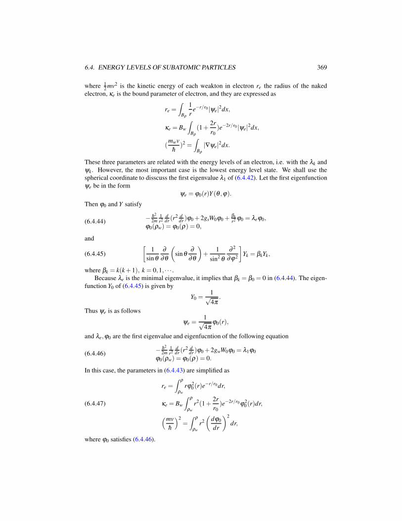
6.4. ENERGY LEVELS OF SUBATOMIC PARTICLES 369
where 12mv2 is the kinetic energy of each weakton in electron re the radius of the naked
electron, κe is the bound parameter of electron, and they are expressed as
re =∫
Bρ
1
re−r/r0 |ψe|2dx,
κe = Bw
∫
Bρ
(1+2r
r0
)e−2r/r0 |ψe|2dx,
(mwv
h)2 =
∫
Bρ
|∇ψe|2dx.
These three parameters are related with the energy levels of an electron, i.e. with the λk and
ψk. However, the most important case is the lowest energy level state. We shall use the
spherical coordinate to disscuss the first eigenvalue λ1 of (6.4.42). Let the first eigenfunction
ψe be in the form
ψe = ϕ0(r)Y (θ ,ϕ).
Then ϕ0 and Y satisfy
(6.4.44)− h2
2m1r2
ddr(r2 d
dr)ϕ0 + 2gsW0ϕ0 +
βk
r2 ϕ0 = λeϕ0,
ϕ0(ρw) = ϕ0(ρ) = 0,
and
(6.4.45)
[1
sin θ
∂
∂θ
(sinθ
∂
∂θ
)+
1
sin2 θ
∂ 2
∂ϕ2
]Yk = βkYk,
where βk = k(k+ 1), k = 0,1, · · · .Because λe is the minimal eigenvalue, it implies that βk = β0 = 0 in (6.4.44). The eigen-
function Y0 of (6.4.45) is given by
Y0 =1√4π
.
Thus ψe is as follows
ψe =1√4π
ϕ0(r),
and λe,ϕ0 are the first eigenvalue and eigenfucntion of the following equation
(6.4.46)− h2
2m1r2
ddr(r2 d
dr)ϕ0 + 2gwW0ϕ0 = λ1ϕ0
ϕ0(ρw) = ϕ0(ρ) = 0.
In this case, the parameters in (6.4.43) are simplified as
re =∫ ρ
ρw
rϕ20 (r)e
−r/r0dr,
κe = Bw
∫ ρ
ρw
r2(1+2r
r0
)e−2r/r0ϕ20 (r)dr,(6.4.47)
(mv
h
)2
=∫ ρ
ρw
r2
(dϕ0
dr
)2
dr,
where ϕ0 satisfies (6.4.46).
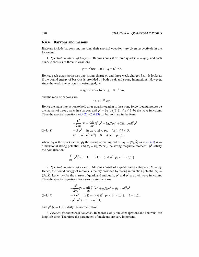
370 CHAPTER 6. QUANTUM PHYSICS
6.4.4 Baryons and mesons
Hadrons include baryons and mesons, their spectral equations are given respectively in the
following.
1. Spectral equations of baryons. Baryons consist of three quarks: B = qqq, and each
quark q consists of three w-weaktons
q = w∗ww and q = w∗ww.
Hence, each quark possesses one strong charge gs and three weak charges 3gw. It looks as
if the bound energy of baryons is provided by both weak and strong interactions. However,
since the weak interaction is short-ranged, i.e.
range of weak force ≤ 10−16 cm,
and the radii of baryons are
r > 10−16 cm.
Hence the main interaction to hold three quarks together is the strong force. Let m1,m2,m3 be
the masses of three quarks in a baryon, and ψk = (ψk1 ,ψ
k2)
T (1≤ k ≤ 3) be the wave functions.
Then the spectral equations (6.4.21)-(6.4.23) for baryons are in the form
− h2
2mk
(∇+ i2gs
hc~s)2ψk + 2gsS0ψk + 2~µk · curl~Sψk
= λ ψk in ρ0 < |x|< ρ1, for 1 ≤ k ≤ 3,(6.4.48)
ψ = (ψ1,ψ2,ψ3) = 0 at |x|= ρ0,ρ1,
where ρ0 is the quark radius, ρ1 the strong attracting radius, Sµ = (S0,~S) as in (6.4.1) is 4-
dimensional strong potential, and ~µk = hgs~σ/2mk the strong magnetic moment. ψk satisfy
the nomalization∫
Ω|ψk|2dx = 1, in Ω = x ∈ R3| ρ0 < |x|< ρ1.
2. Spectral equations of mesons. Mesons consist of a quark and a antiquark: M = qq.
Hence, the bound energy of mesons is mainly provided by strong interaction potential Sµ =
(S0,~S). Let m1,m2 be the masses of quark and antiquark, ψ1 and ψ2 are their wave functions.
Then the spectral equations for mesons take the form
− h2
2mk
(∇+ igs
hc~S)2ψk + gsS0ψk +~µk · curl~Sψk
= λ ψk in Ω = x ∈ R3| ρ0 < |x|< ρ1, k = 1,2,(6.4.49)
(ψ1,ψ2) = 0 on ∂Ω,
and ψk (k = 1,2) satisfy the normalization.
3. Physical parameters of nucleons. In hadrons, only nucleons (protons and neutrons) are
long life-time. Therefore the parameters of nucleons are very important.
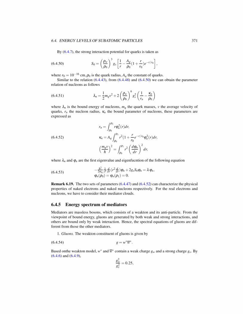
6.4. ENERGY LEVELS OF SUBATOMIC PARTICLES 371
By (6.4.7), the strong interaction potential for quarks is taken as
(6.4.50) S0 =
(ρw
ρ0
)3
gs
[1
r− Aq
ρ0
(1+r
r0
)e−r/r0
],
where r0 = 10−16 cm,ρ0 is the quark radius, Aq the constant of quarks.
Similar to the relation (6.4.43), from (6.4.48) and (6.4.50) we can obtain the parameter
relation of nucleons as follows
(6.4.51) λn =1
2mqv2 + 2
(ρw
ρ0
)6
g2s
(1
rn
− κn
ρ0
)
where λn is the bound energy of nucleons, mq the quark masses, v the average velocity of
quarks, rn the nucleon radius, κn the bound parameter of nucleons, these parameters are
expressed as
rn =
∫ ρ1
ρ0
rϕ2n (r)dr,
κn = Aq
∫ ρ1
ρ0
r2(1+r
r0
e−r/r0ϕ2n (r)dr,(6.4.52)
(mqv
h
)2
=
∫ ρ1
ρ0
r2
(dϕn
dr
)2
dr,
where λn and ϕn are the first eigenvalue and eigenfucntion of the following equation
(6.4.53)− h2
2mq
1r2
ddr(r2 d
dr)ϕn + 2gsS0ϕn = λ ϕn,
ϕn(ρ0) = ϕn(ρ1) = 0.
Remark 6.19. The two sets of parameters (6.4.47) and (6.4.52) can characterize the physical
properties of naked electrons and naked nucleons respectively. For the real electrons and
nucleons, we have to consider their mediator clouds.
6.4.5 Energy spectrum of mediators
Mediators are massless bosons, which consists of a weakton and its anti-particle. From the
viewpoint of bound energy, gluons are generated by both weak and strong interactions, and
others are bound only by weak interaction. Hence, the spectral equations of gluons are dif-
ferent from those the other mediators.
1. Gluons. The weakton constituent of gluons is given by
(6.4.54) g = w∗w∗.
Based onthe weakton model, w∗ and w∗ contain a weak charge gw and a strong charge gs. By
(6.4.6) and (6.4.9),
g2w
g2s
= 0.25,
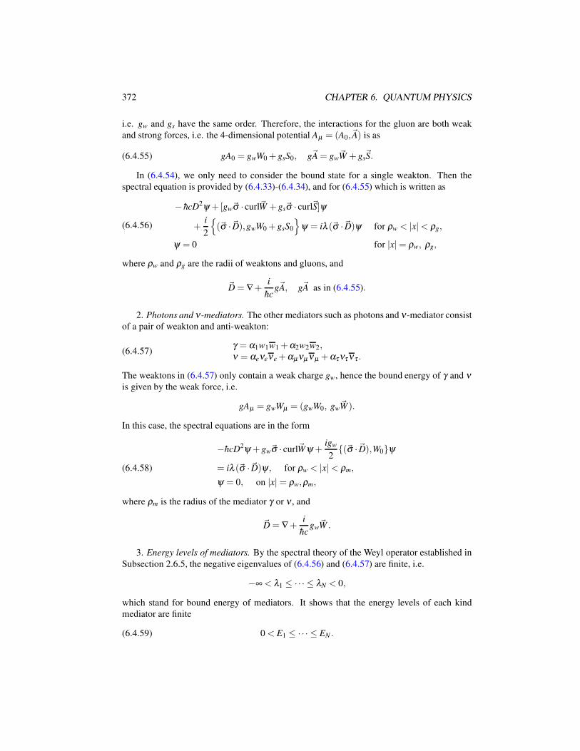
372 CHAPTER 6. QUANTUM PHYSICS
i.e. gw and gs have the same order. Therefore, the interactions for the gluon are both weak
and strong forces, i.e. the 4-dimensional potential Aµ = (A0,~A) is as
(6.4.55) gA0 = gwW0 + gsS0, g~A = gw~W + gs
~S.
In (6.4.54), we only need to consider the bound state for a single weakton. Then the
spectral equation is provided by (6.4.33)-(6.4.34), and for (6.4.55) which is written as
(6.4.56)
− hcD2ψ +[gw~σ · curl~W + gs~σ · curl~S]ψ
+i
2
(~σ ·~D),gwW0 + gsS0
ψ = iλ (~σ ·~D)ψ for ρw < |x|< ρg,
ψ = 0 for |x|= ρw, ρg,
where ρw and ρg are the radii of weaktons and gluons, and
~D = ∇+i
hcg~A, g~A as in (6.4.55).
2. Photons and ν-mediators. The other mediators such as photons and ν-mediator consist
of a pair of weakton and anti-weakton:
(6.4.57)γ = α1w1w1 +α2w2w2,ν = αeνeνe +αµνµ νµ +ατντ ντ .
The weaktons in (6.4.57) only contain a weak charge gw, hence the bound energy of γ and νis given by the weak force, i.e.
gAµ = gwWµ = (gwW0, gw~W ).
In this case, the spectral equations are in the form
−hcD2ψ + gw~σ · curl~Wψ +igw
2(~σ ·~D),W0ψ
= iλ (~σ ·~D)ψ , for ρw < |x|< ρm,(6.4.58)
ψ = 0, on |x|= ρw,ρm,
where ρm is the radius of the mediator γ or ν , and
~D = ∇+i
hcgw
~W .
3. Energy levels of mediators. By the spectral theory of the Weyl operator established in
Subsection 2.6.5, the negative eigenvalues of (6.4.56) and (6.4.57) are finite, i.e.
−∞ < λ1 ≤ ·· · ≤ λN < 0,
which stand for bound energy of mediators. It shows that the energy levels of each kind
mediator are finite
(6.4.59) 0 < E1 ≤ ·· · ≤ EN .
6.4. ENERGY LEVELS OF SUBATOMIC PARTICLES 373
Each energy level Ek can be expressed as
(6.4.60) Ek = E0 +λk (1 ≤ k ≤ N),
where E0 is the intrinsic energy of mediators.
It follows from (6.4.59) and (6.4.60) that the frequencies of mediators are finite and dis-
crete
(6.4.61) ωk =1
hEk (1 ≤ k ≤ N),
and the difference of two adjacent frequencies is
(6.4.62) ∆ωk = ωk+1 −ωk =1
h(λk+1 −λk).
Remark 6.20. In the classical quantum mechanics, the frequencies of particles are continu-
ously distributed. Here we derive from the energy spectrum theory that the frequencies are
finite and discrete. In fact, by the estimate (3.6.51) of the number of negative eigenvalues, we
can verify that the frequency difference (6.4.62) is too small to measure in the next subsection.
6.4.6 Discreteness of energy spectrum
Based on the spectral theory developed in Section 3.6, the energy levels of all subatomic
particles are finite and discrete:
(6.4.63) 0 < E1 < · · ·< EN ,
where the number N of energy levels depends on the particle type. Each subatomic particle
lies in an energy state of Ek (1 ≤ k ≤ N) in (6.4.63). In traditional conception, the energy
distribution of all particles is infinite and continuous, i.e. a particle can lie in any state of
energy E with 0 < E < ∞. Hence the energy level theory established here arrive at a very
different conclution:
Physical Conclusion 6.21. The energy distribution of subatomic particles is finite and dis-
crete.
Usually, we cannot observe the discreteness of energy because the number N of energy
levels is so large that the average difference of adjacent energy level:
∆Ek = Ek+1 −Ek ≃EN −E1
N≃ 0,
is very small. In the following discussion we shall show this point.
To this end, we first give the estimates of the number N of energy levels for various types
of subatomic particles.
1. Energy level number of electrons and quarks. To consider the approximatively com-
putation of number N of energy levels, we always ignore the magnetic effects. In this case,
374 CHAPTER 6. QUANTUM PHYSICS
the spectral equations for charged leptons and quarks are given by (6.4.42), and which are
written as
(6.4.64)− h2
2mw∆ψ + 2gwW0ψ = λ ψ in ρw < |x|< ρ ,
ψ = 0, on |x|= ρw,ρ ,
where mw is the masses of weaktons in leptons and quarks, ρ is the attracting radius of weak
interaction.
For the weak interaction potential W0, we approximatively take
W0 =−gwBw
ρw
.
Then take the dimensional transformation
x → ρx (ρ as in (6.4.64)).
Note that the weakton radius ρw for smaller than ρ ,
ρw ≪ ρ .
Hence, the problem (6.4.64) can be approximatively expressed as
(6.4.65)−∆ψ − 4mwBwρ2
h2ρwg2
wψ = λ ψ for |x|< 1,
ψ = 0 on |x|= 1.
It is clear that for the equation (6.4.65), the parameters r,α,θ as in (3.6.28) of Theorem
2.37 are as follows
r = 1, α = 0, θ =4mwBwρ2
h2ρw
g2w
Thus the number N of the energy levels of charged leptons and quarks is approximatively
given by
(6.4.66) N =
[4
λ1
Bwρ2
ρw
mwc
h
g2w
hc
] 32
,
where λ1 is the first eigenvalue of −∆ in unit ball B1 ⊂ R3.
By the de Broglie relation,mwc
h∼ 1
6 λ ,
where 6 λ is the wave length of weaktons, i.e. 6 λ = nrm (n = 1,2, · · ·),rm the mediator radius.
We take 6 λ = rm ≃ ρ , and
4
λ1
≃ 1,Bwρ
ρw
≃ 102,mwc
hρ ≃ 1.
Then, by (6.4.6) the number N in (6.4.66) has the estimate
(6.4.67) N ∼(
ρn
ρw
)9
≥ 1045.
6.4. ENERGY LEVELS OF SUBATOMIC PARTICLES 375
This number is very large because (ρn/ρw)≥ 105.We remark that the estimate (6.4.67) only for the naked leptons and quarks. For the
natural leptons and quarks, their energy level number N should take as
N = N ·N1,
where N is as in (6.4.67) and N1 the energy level number of mediator cloud around the
charged leptons and quarks.
2. Energy level number of hadrons. We only consider the case of baryons, and the case of
mesons is similar. For the baryons, spectral equation (6.4.48) can be approximatively reduced
in the form
(6.4.68)−∆ψ − 4mqAqρ2
1
h2ρqg2
s ψ = λ ψ , for |x|< 1,
ψ = 0, on |x|= 1.
where mq is the quark mass, ρq the quark radius, ρ1 the strong attracting radius, and Aq the
strong interaction constant of quarks.
By Theorem 3.38, from (6.4.68) we can get the estimates of energy level number N of
baryons as follows
(6.4.69) N =
[4
λ1
ρ21 Aq
ρq
mqc
h
g2s
hc
] 32
,
where λ1 is as in (6.4.66). By (6.4.69) and (6.4.9) we can get the same estimate as in (6.4.67).
3. Energy level number of mediators. Likewise, we only consider the energy level number
of photons. In this case, the spectral equation (6.4.58) can be reduced as
(6.4.70)−∆ϕ = i(λ + Bwρr
hcρwg2
w)(~σ ·∇)ϕ , for |x|< 1,
ϕ = 0 on |x|= 1,
where ργ is the photon radius.
By (6.4.70) we can see that the parameter K as in (3.6.51) takes
K =Bwργ
ρw
g2w
hc.
Thus, by (3.6.51) the energy level number N of photons is given by
(6.4.71) N =
(K
β1
)3
=
[1
β1
Bwργ
ρw
g2w
hc
]3
,
where β1 is as in (3.6.51), and β1 ∼ o(1).From the physical significance, ργ is approximatively the weak attracting radius of weak-
tons, and ρw/Bw = ρ satisfying
Fw
> 0 for 0 < r < ρ,< 0 for ρ < r < ργ .
376 CHAPTER 6. QUANTUM PHYSICS
Hence, it is natural to think that
Bwργ
ρw
=ργ
ρ= 102 ∼ 104.
Thus, by (6.4.71) and (6.4.6) we get hat
(6.4.72) N ∼(
ρn
ρw
)18
≥ 1090.
Remark 6.22. In the estimates (6.4.66), (6.4.69) and (6.4.71), the energy level numbers N
for various subatomic particles are counting the multiplicities of eigenvalues. However, the
numbers N have the same order as the real energy level numbers. It is because that the
multiple eigenvalues are unstable, under the perturbation of electromagnetism together with
weak and strong magnetism, most multiple eigenvalues become the simple eigenvalues.
4. Energy level gradient of photons. Each energy level Ek (1 ≤ k ≤ N) of photons can be
written as
Ek = E0 +λk (1 ≤ k ≤ N).
It is clear that the largest and smallest energy levels are given by
Emax = E0 +λN , Emin = E0 +λ1.
The total energy level difference is
Emax −Emin = λN −λ1.
Since |λ1| ≫ |λN |, the average energy level gradient (for two adjacent energy levels) is ap-
proximatively given by
(6.4.73) ∆E =Emax −Emin
N≃ |λ1|
N.
The first eigenvalue λ1 of (6.4.70) is
λ1 ≃−K
(the unit is
hc
ργ
).
Hence, by (6.4.71) and (6.4.73)
∆E = β 31 K−2 hc
ργ, K =
Bwργ
ρw
g2w
hc.
Then we get the estimates
(6.4.74) ∆E =
(ρw
ρn
)12hc
ργ.
As we takeρw
ρn
= 10−5, ργ = 10−20cm,
6.5. FIELD THEORY OF MULTI-PARTICLE SYSTEMS 377
then from (6.4.74) we derive that
∆E = 10−40hc/ cm = 2× 10−45eV.
This is a very small value, and it is impossible for experiments to measure.
Remark 6.23. The physical conclusion that all particles have finite and discrete energy dis-
tribution is of very important significance for the quantum field theory. It implies that the
infinity appearing in the field quantization does not exist, and the renormalization theory
needs to be reconsidered.
6.5 Field Theory of Multi-Particle Systems
6.5.1 Introduction
We start with the known model of multi-particle systems. Consider an N-particle system with
particles
(6.5.1) A1, · · · ,AN .
Let xk = (x1k ,x
2k ,x
3k) ∈ R3 be the coordinate of Ak, and
(6.5.2) ψ = ψ(t,x1, · · · ,xk)
be the wave function describing the N-particle system (6.5.1). Then, the classical theory for
(6.5.1) is provided by the Schrodinger equation
(6.5.3) ih∂ψ
∂ t=−
N
∑k=1
h2
2mk
∆kψ + ∑j 6=k
V (x j,xk)ψ ,
where V (x j,xk) is the potential energy of interactions between A j and Ak, mk is the mass of
Ak, and
∆k =∂ 2
(∂x1k)
2+
∂ 2
(∂x2k)
2+
∂ 2
(∂x3k)
2.
The wave function ψ satisfies the normalization condition
∫
R3· · ·∫
R3|ψ |2dx1 · · ·dxN = 1.
Namely, the physically |ψ(t,x1, · · · ,xN)|2 represents the probability density of A1, · · · ,AN
appearing at x1, · · · ,xN at time t.
It is clear that the Schrodinger equation (6.5.3) for an N-particle system is only an ap-
proximate model:
• It is non-relativistic model;
• The model does not involve the vector potentials~A of the interactions between particles.
378 CHAPTER 6. QUANTUM PHYSICS
• By using coordinate xk to represent the particle Ak amounts essentially to saying that
the wave function ψ satisfying (6.5.3) can only describe the statistic properties of the
system (6.5.1), and contains no information for each individual particle Ak (1≤ k ≤N).
• The model is decoupled with interaction fields, i.e. the interaction fields in the model
are treated as given functions.
In fact, the most remarkable characteristic of interacting multi-particle systems is that
both particle fields and interaction fields are closely related. Therefore, a complete field
model of multi-particle systems have to couple both the particle field equations and the inter-
action field equations. In particular, a precise unified field theory should be based on the field
model of the multi-particle system coupled with the four fundamental interactions.
6.5.2 Basic postulates for N-body quantum physics
As mentioned in the last subsection, the dynamic models for multi-particle quantum systems
have to couple both particle and interaction fields. Therefore there should be some added
quantum rules for the systems. In the following we propose the basic postulates for N-particle
quantum systems.
First of all, the physical systems have to satisfy a few fundamental physical principles
introduced below.
Postulate 6.24. Any N-particle quantum system has to obey the physical fundamental prin-
ciples such as:
(6.5.4)
Einstein General Relativity,
Lorentz Invariance,
Gauge Invariance,
Gauge Representation Invariance (PRI),
Principle of Lagrange Dynamics (PLD),
Principle of Interaction Dynamics (PID),
where the gauge invariance means the invariance of the Lagrangian action under corre-
sponding gauge transformations.
We note that in general multi-particle systems are layered, and may consist of numerous
sub-systems. In particular, we know that the weak and strong interactions are also layered.
Hence, here we consider the same level systems, i.e. the systems which consist of identical
particles or sub-systems possessing the same level of interactions.
For multi-particle systems with N same level subsystems Ak (1 ≤ k ≤ N), the energy
contributions of Ak are indistinguishable. Hence, the Lagrangian actions for the N-particle
systems satisfy SU(N) gauge invariance. Thus we propose the following basic postulate:
Postulate 6.25. An N-particle system obeys the SU(N) gauge invariance, i.e. the Lagrangian
action of this system is invariant under the SU(N) gauge transformation
(6.5.5)
ψ1
...
ψN
= Ω
ψ1
...
ψN
, Ω ∈ SU(N),
6.5. FIELD THEORY OF MULTI-PARTICLE SYSTEMS 379
where ψ1, · · · ,ψN are the wave functions of the N particles.
We now need to explain the physical significance of the SU(N) gauge fields induced by
Postulate 6.25.
Let each particle of the N-particle system carry an interaction charge g (for example a
weak charge g = gw). Then, there are interactions present between the N particles. By the
SU(N) gauge theory, the gauge invariant 4-dimensional energy-momentum operator is given
by
(6.5.6) Dµ = ∂µ + igGaµτa for 1 ≤ a ≤ N2 − 1,
and the interaction energy generated by the N particles is
(6.5.7) E =
Ψ(iγµDµΨ) for fermions,
|DµΨ|2 for bosons,
where Ψ = (ψ1, · · · ,ψN)T , and Dµ is as in (6.5.6). From (6.5.6) and (6.5.7) we obtain the
physical explanation to the SU(N) gauge fields Gaµ , stated in the following postulate:
Postulate 6.26. For a system of N-particles in the same level with each particle carrying
an interaction charge g, the N particles induce dynamic interactions between them, and the
SU(N) gauge fields
(6.5.8) gGaµ for 1 ≤ a ≤ N2 − 1
stand for the interaction potentials between the N particles.
The N particles induce dynamic interactions between them in terms of the SU(N) gauge
fields (6.5.8). These interaction fields cannot be measured experimentally because they de-
pend on the choice of generator representation τa of SU(N). By the SU(N) geometric theory
in Section 3.5, there is a constant SU(N) tensor
(6.5.9) αNa = (αN
1 , · · · ,αNN ),
such that the contraction field using PRI
(6.5.10) Gµ = αNa Ga
is independent of the SU(N) representation τa. The field (6.5.10) is the interaction field which
can be experimentally observed. Thus we propose the following basic postulate.
Postulate 6.27. For an N-particle system, only the interaction field given by (6.5.10) can be
measured, and is the interaction field under which this system interacts with other external
systems.
Remark 6.28. Postulates 6.24-6.27, together with the Principle of Symmetry-Breaking 2.14
and the Postulates 6.1-6.5, form a complete foundation for quantum physics. In fact, without
Postulates 6.24-6.27, we cannot establish the quantum physics of multi-particle systems.
380 CHAPTER 6. QUANTUM PHYSICS
The main motivation to introduce Postulates 6.25 and 6.26 are as follows. Consider an
N-particle system with each particle carrying an interaction charge g. Let this be a fermionic
system, and the Dirac spinors be given by
Ψ = (ψ1, · · · ,ψN)T .
By Postulates 6.3 and 6.5, the Dirac equations for this system can be expressed in the general
form
(6.5.11) iγµDµΨ+MΨ = 0,
where M is the mass matrix, and
(6.5.12) DµΨ = ∂µ
ψ1
...
ψN
+ ig
G11µ · · · G1N
µ...
...
GN1µ · · · GNN
µ
ψ1
...
ψN
,
where G = (Gi jµ ) is an Hermitian matrix, representing the interaction potentials between the
N particles generated by the interaction charge g.
Notice that the space consisting of all Hermitian matrices
H(N) = G| G is an N-th order Hermitian matrix
is an N2−dimensional linear space with basis
(6.5.13) τ0, τ1, · · · , τK with K = N2 − 1,
where τ0 = I is the identity, and τa (1 ≤ a ≤ N2 − 1) are the traceless Hermitian matrices.
Hence, the Hermitian matrix G = (Gi jµ ) ∈ H(N) in (6.5.12) can be expressed as
G = G0µ I +Ga
µτa with τa as in (6.5.13).
Thus, the differential operator in (6.5.12) is in the form
(6.5.14) Dµ = ∂µ + igG0µ + igGa
µτa.
The equations (6.5.11) with (6.5.14) are just the Dirac equations in the form of SU(N)gauge fields Ga
µ | 1 ≤ a ≤ N2 − 1 with a given external interaction field G0µ . Thus, based
on Postulate 6.24, the gauge invariance of an N-particle system and the expressions (6.5.11)
and (6.5.14) of the N fermionic particle field equations dictate Postulates 6.25 and 6.26.
The derivation here indicates that Postulates 6.25 and 6.26 can be considered as the conse-
quence of 1) the gauge invariance stated in Postulate 6.24, and 2) the existence of interactions
between particles as stated in (6.5.12), which can be considered as an axiom.
6.5.3 Field equations of multi-particle systems
Based on the basic axioms given by Postulates 6.24-6.27, we can establish field equations for
various levels of N-particle systems. We proceed in several different cases.
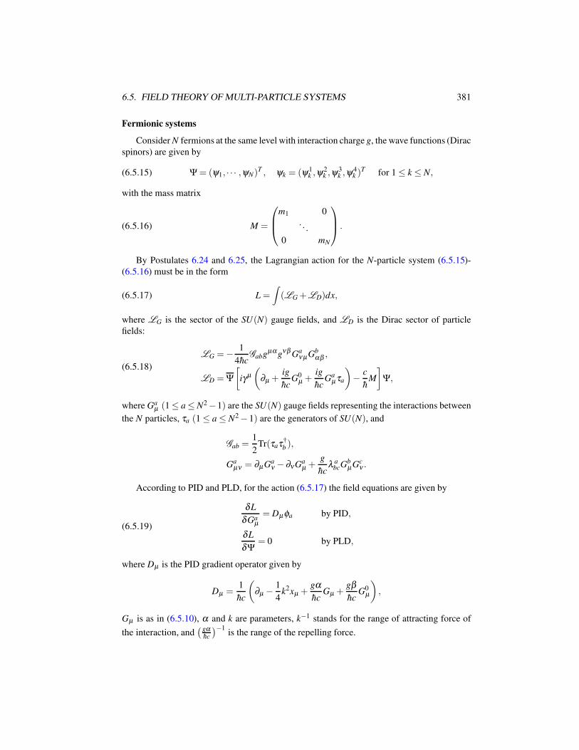
6.5. FIELD THEORY OF MULTI-PARTICLE SYSTEMS 381
Fermionic systems
Consider N fermions at the same level with interaction charge g, the wave functions (Dirac
spinors) are given by
(6.5.15) Ψ = (ψ1, · · · ,ψN)T , ψk = (ψ1
k ,ψ2k ,ψ
3k ,ψ
4k )
T for 1 ≤ k ≤ N,
with the mass matrix
(6.5.16) M =
m1 0
. . .
0 mN
.
By Postulates 6.24 and 6.25, the Lagrangian action for the N-particle system (6.5.15)-
(6.5.16) must be in the form
(6.5.17) L =∫(LG +LD)dx,
where LG is the sector of the SU(N) gauge fields, and LD is the Dirac sector of particle
fields:
(6.5.18)
LG =− 1
4hcGabgµαgνβ Ga
νµGbαβ ,
LD = Ψ
[iγµ
(∂µ +
ig
hcG0
µ +ig
hcGa
µτa
)− c
hM
]Ψ,
where Gaµ (1 ≤ a ≤ N2 −1) are the SU(N) gauge fields representing the interactions between
the N particles, τa (1 ≤ a ≤ N2 − 1) are the generators of SU(N), and
Gab =1
2Tr(τaτ†
b ),
Gaµν = ∂µGa
ν − ∂νGaµ +
g
hcλ a
bcGbµGc
ν .
According to PID and PLD, for the action (6.5.17) the field equations are given by
(6.5.19)
δL
δGaµ
= Dµφa by PID,
δL
δΨ= 0 by PLD,
where Dµ is the PID gradient operator given by
Dµ =1
hc
(∂µ − 1
4k2xµ +
gα
hcGµ +
gβ
hcG0
µ
),
Gµ is as in (6.5.10), α and k are parameters, k−1 stands for the range of attracting force of
the interaction, and(
gαhc
)−1is the range of the repelling force.
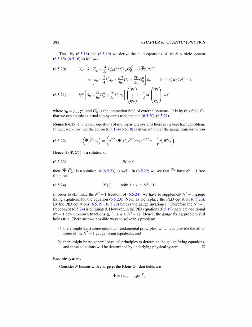
382 CHAPTER 6. QUANTUM PHYSICS
Thus, by (6.5.18) and (6.5.19) we derive the field equations of the N-particle system
(6.5.15)-(6.5.16) as follows
Gab
[∂ ν Gb
νµ − g
hcλ b
cdgαβ GcαµGd
β
]− gΨγµ τaΨ(6.5.20)
=
[∂µ −
1
4k2xµ +
gα
hcGµ +
gβ
hcG0
µ
]φa for 1 ≤ a ≤ N2 − 1,
iγµ
[∂µ +
ig
hcG0
µ +ig
hcGa
µτa
]
ψ1
...
ψN
− c
hM
ψ1
...
ψN
= 0,(6.5.21)
where γµ = gµνγν , and G0µ is the interaction field of external systems. It is by this field G0
µ
that we can couple external sub-systems to the model (6.5.20)-(6.5.21).
Remark 6.29. In the field equations of multi-particle systems there is a gauge fixing problem.
In fact, we know that the action (6.5.17)-(6.5.18) is invariant under the gauge transformation
(6.5.22)(
Ψ, Gaµτa
)=
(eiθ aτaΨ,Ga
µeiθ bτb τae−iθ bτb − 1
g∂µθ bτb
).
Hence if (Ψ,Gaµ) is a solution of
(6.5.23) δL = 0,
then (Ψ, Gaµ) is a solution of (6.5.23) as well. In (6.5.22) we see that Ga
µ have N2 − 1 free
functions
(6.5.24) θ a(x) with 1 ≤ a ≤ N2 − 1.
In order to eliminate the N2 − 1 freedom of (6.5.24), we have to supplement N2 − 1 gauge
fixing equations for the equation (6.5.23). Now, as we replace the PLD equation (6.5.23).
By the PID equations (6.5.19), (6.5.22) breaks the gauge invariance. Therefore the N2 − 1
freedom of (6.5.24) is eliminated. However, in the PID equations (6.5.19) there are additional
N2 − 1 new unknown functions φa (1 ≤ a ≤ N2 − 1). Hence, the gauge fixing problem still
holds true. There are two possible ways to solve this problem:
1) there might exist some unknown fundamental principles, which can provide the all or
some of the N2 − 1 gauge fixing equations; and
2) there might be no general physical principles to determine the gauge fixing equations,
and these equations will be determined by underlying physical system.
Bosonic systems
Consider N bosons with charge g, the Klein-Gordon fields are
Φ = (ϕ1, · · · ,ϕN)T ,
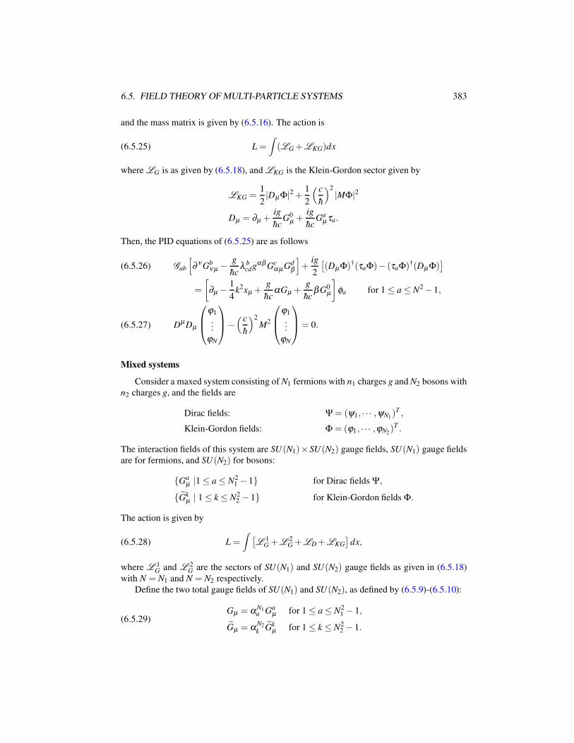
6.5. FIELD THEORY OF MULTI-PARTICLE SYSTEMS 383
and the mass matrix is given by (6.5.16). The action is
(6.5.25) L =
∫(LG +LKG)dx
where LG is as given by (6.5.18), and LKG is the Klein-Gordon sector given by
LKG =1
2|DµΦ|2 + 1
2
( c
h
)2
|MΦ|2
Dµ = ∂µ +ig
hcG0
µ +ig
hcGa
µ τa.
Then, the PID equations of (6.5.25) are as follows
Gab
[∂ νGb
νµ − g
hcλ b
cdgαβ GcαµGd
β
]+
ig
2
[(DµΦ)†(τaΦ)− (τaΦ)†(DµΦ)
](6.5.26)
=
[∂µ − 1
4k2xµ +
g
hcαGµ +
g
hcβ G0
µ
]φa for 1 ≤ a ≤ N2 − 1,
DµDµ
ϕ1
...
ϕN
−
( c
h
)2
M2
ϕ1
...
ϕN
= 0.(6.5.27)
Mixed systems
Consider a maxed system consisting of N1 fermions with n1 charges g and N2 bosons with
n2 charges g, and the fields are
Dirac fields: Ψ = (ψ1, · · · ,ψN1)T ,
Klein-Gordon fields: Φ = (ϕ1, · · · ,ϕN2)T .
The interaction fields of this system are SU(N1)×SU(N2) gauge fields, SU(N1) gauge fields
are for fermions, and SU(N2) for bosons:
Gaµ |1 ≤ a ≤ N2
1 − 1 for Dirac fields Ψ,
Gkµ | 1 ≤ k ≤ N2
2 − 1 for Klein-Gordon fields Φ.
The action is given by
(6.5.28) L =
∫ [L
1G +L
2G +LD+LKG
]dx,
where L 1G and L 2
G are the sectors of SU(N1) and SU(N2) gauge fields as given in (6.5.18)
with N = N1 and N = N2 respectively.
Define the two total gauge fields of SU(N1) and SU(N2), as defined by (6.5.9)-(6.5.10):
(6.5.29)Gµ = αN1
a Gaµ for 1 ≤ a ≤ N2
1 − 1,
Gµ = αN2k
Gkµ for 1 ≤ k ≤ N2
2 − 1.
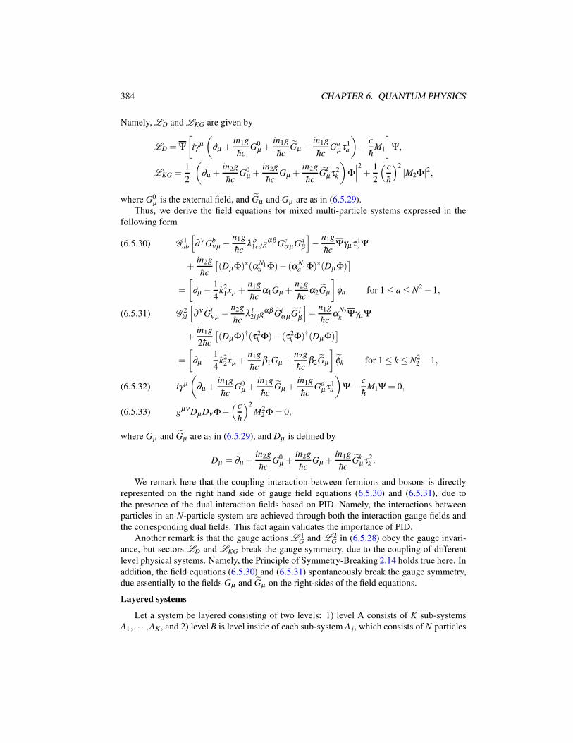
384 CHAPTER 6. QUANTUM PHYSICS
Namely, LD and LKG are given by
LD = Ψ
[iγµ
(∂µ +
in1g
hcG0
µ +in1g
hcGµ +
in1g
hcGa
µτ1a
)− c
hM1
]Ψ,
LKG =1
2
∣∣∣(
∂µ +in2g
hcG0
µ +in2g
hcGµ +
in2g
hcGk
µτ2k
)Φ∣∣∣2
+1
2
( c
h
)2
|M2Φ|2,
where G0µ is the external field, and Gµ and Gµ are as in (6.5.29).
Thus, we derive the field equations for mixed multi-particle systems expressed in the
following form
G1ab
[∂ ν Gb
νµ −n1g
hcλ b
1cdgαβ GcαµGd
β
]− n1g
hcΨγµτ1
a Ψ(6.5.30)
+in2g
hc
[(DµΦ)∗(αN1
a Φ)− (αN1a Φ)∗(Dµ Φ)
]
=
[∂µ −
1
4k2
1xµ +n1g
hcα1Gµ +
n2g
hcα2Gµ
]φa for 1 ≤ a ≤ N2 − 1,
G2kl
[∂ ν Gl
νµ − n2g
hcλ l
2i jgαβ Gi
αµGj
β
]− n1g
hcαN2
k Ψγµ Ψ(6.5.31)
+in1g
2hc
[(DµΦ)†(τ2
k Φ)− (τ2k Φ)†(DµΦ)
]
=
[∂µ −
1
4k2
2xµ +n1g
hcβ1Gµ +
n2g
hcβ2Gµ
]φk for 1 ≤ k ≤ N2
2 − 1,
iγµ
(∂µ +
in1g
hcG0
µ +in1g
hcGµ +
in1g
hcGa
µτ1a
)Ψ− c
hM1Ψ = 0,(6.5.32)
gµνDµDν Φ−(c
h
)2
M22 Φ = 0,(6.5.33)
where Gµ and Gµ are as in (6.5.29), and Dµ is defined by
Dµ = ∂µ +in2g
hcG0
µ +in2g
hcGµ +
in1g
hcGk
µτ2k .
We remark here that the coupling interaction between fermions and bosons is directly
represented on the right hand side of gauge field equations (6.5.30) and (6.5.31), due to
the presence of the dual interaction fields based on PID. Namely, the interactions between
particles in an N-particle system are achieved through both the interaction gauge fields and
the corresponding dual fields. This fact again validates the importance of PID.
Another remark is that the gauge actions L 1G and L 2
G in (6.5.28) obey the gauge invari-
ance, but sectors LD and LKG break the gauge symmetry, due to the coupling of different
level physical systems. Namely, the Principle of Symmetry-Breaking 2.14 holds true here. In
addition, the field equations (6.5.30) and (6.5.31) spontaneously break the gauge symmetry,
due essentially to the fields Gµ and Gµ on the right-sides of the field equations.
Layered systems
Let a system be layered consisting of two levels: 1) level A consists of K sub-systems
A1, · · · ,AK , and 2) level B is level inside of each sub-system A j, which consists of N particles
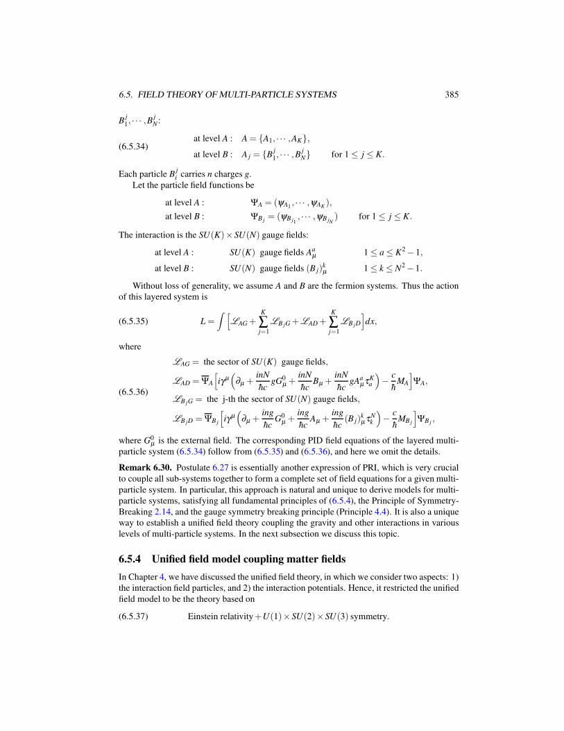
6.5. FIELD THEORY OF MULTI-PARTICLE SYSTEMS 385
Bj1, · · · ,B
jN :
(6.5.34)at level A : A = A1, · · · ,AK,at level B : A j = B
j1, · · · ,B
jN for 1 ≤ j ≤ K.
Each particle Bji carries n charges g.
Let the particle field functions be
at level A : ΨA = (ψA1, · · · ,ψAK
),
at level B : ΨB j= (ψB j1
, · · · ,ψB jN) for 1 ≤ j ≤ K.
The interaction is the SU(K)× SU(N) gauge fields:
at level A : SU(K) gauge fields Aaµ 1 ≤ a ≤ K2 − 1,
at level B : SU(N) gauge fields (B j)kµ 1 ≤ k ≤ N2 − 1.
Without loss of generality, we assume A and B are the fermion systems. Thus the action
of this layered system is
(6.5.35) L =
∫ [LAG +
K
∑j=1
LB jG +LAD+K
∑j=1
LB jD
]dx,
where
(6.5.36)
LAG = the sector of SU(K) gauge fields,
LAD = ΨA
[iγµ(
∂µ +inN
hcgG0
µ +inN
hcBµ +
inN
hcgAa
µτKa
)− c
hMA
]ΨA,
LB jG = the j-th the sector of SU(N) gauge fields,
LB jD = ΨB j
[iγµ(
∂µ +ing
hcG0
µ +ing
hcAµ +
ing
hc(B j)
kµ τN
k
)− c
hMB j
]ΨB j
,
where G0µ is the external field. The corresponding PID field equations of the layered multi-
particle system (6.5.34) follow from (6.5.35) and (6.5.36), and here we omit the details.
Remark 6.30. Postulate 6.27 is essentially another expression of PRI, which is very crucial
to couple all sub-systems together to form a complete set of field equations for a given multi-
particle system. In particular, this approach is natural and unique to derive models for multi-
particle systems, satisfying all fundamental principles of (6.5.4), the Principle of Symmetry-
Breaking 2.14, and the gauge symmetry breaking principle (Principle 4.4). It is also a unique
way to establish a unified field theory coupling the gravity and other interactions in various
levels of multi-particle systems. In the next subsection we discuss this topic.
6.5.4 Unified field model coupling matter fields
In Chapter 4, we have discussed the unified field theory, in which we consider two aspects: 1)
the interaction field particles, and 2) the interaction potentials. Hence, it restricted the unified
field model to be the theory based on
(6.5.37) Einstein relativity+U(1)× SU(2)× SU(3) symmetry.
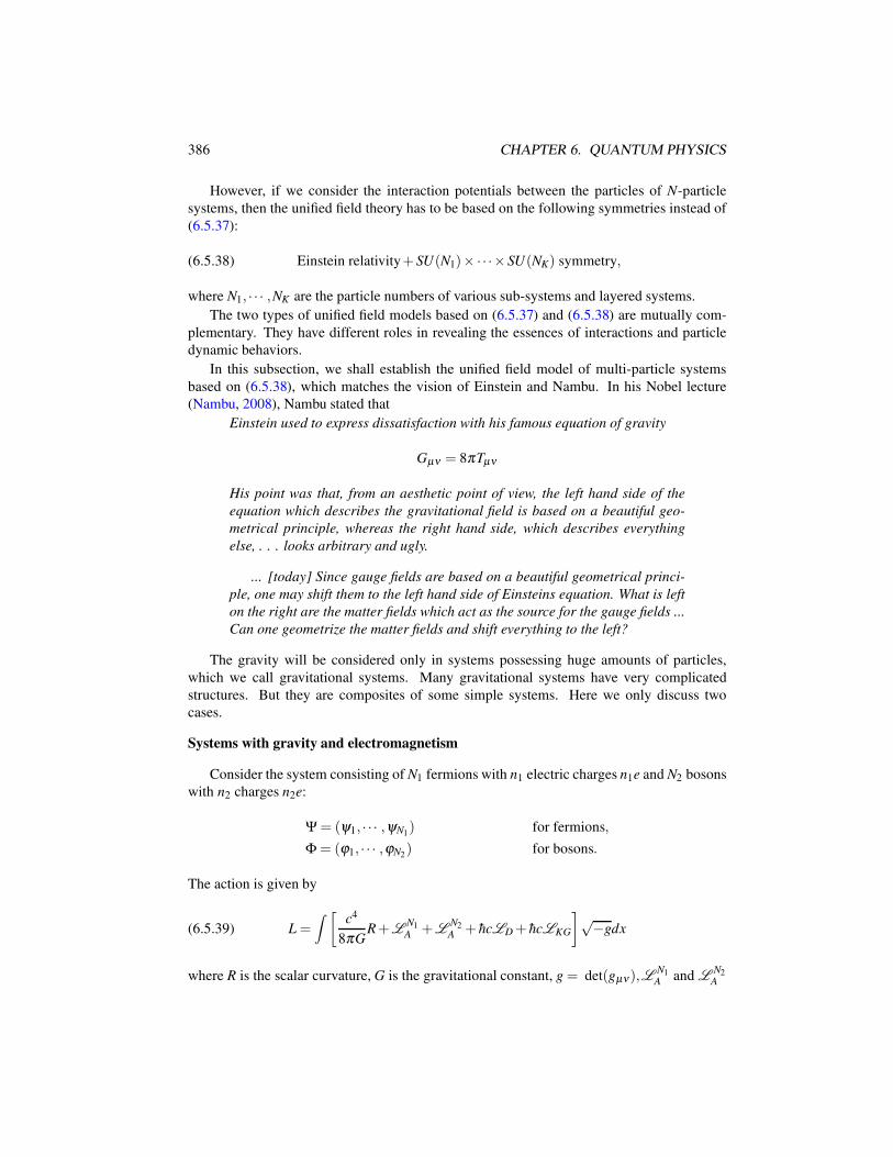
386 CHAPTER 6. QUANTUM PHYSICS
However, if we consider the interaction potentials between the particles of N-particle
systems, then the unified field theory has to be based on the following symmetries instead of
(6.5.37):
(6.5.38) Einstein relativity+ SU(N1)×·· ·× SU(NK) symmetry,
where N1, · · · ,NK are the particle numbers of various sub-systems and layered systems.
The two types of unified field models based on (6.5.37) and (6.5.38) are mutually com-
plementary. They have different roles in revealing the essences of interactions and particle
dynamic behaviors.
In this subsection, we shall establish the unified field model of multi-particle systems
based on (6.5.38), which matches the vision of Einstein and Nambu. In his Nobel lecture
(Nambu, 2008), Nambu stated that
Einstein used to express dissatisfaction with his famous equation of gravity
Gµν = 8πTµν
His point was that, from an aesthetic point of view, the left hand side of the
equation which describes the gravitational field is based on a beautiful geo-
metrical principle, whereas the right hand side, which describes everything
else, . . . looks arbitrary and ugly.
... [today] Since gauge fields are based on a beautiful geometrical princi-
ple, one may shift them to the left hand side of Einsteins equation. What is left
on the right are the matter fields which act as the source for the gauge fields ...
Can one geometrize the matter fields and shift everything to the left?
The gravity will be considered only in systems possessing huge amounts of particles,
which we call gravitational systems. Many gravitational systems have very complicated
structures. But they are composites of some simple systems. Here we only discuss two
cases.
Systems with gravity and electromagnetism
Consider the system consisting of N1 fermions with n1 electric charges n1e and N2 bosons
with n2 charges n2e:
Ψ = (ψ1, · · · ,ψN1) for fermions,
Φ = (ϕ1, · · · ,ϕN2) for bosons.
The action is given by
(6.5.39) L =
∫ [c4
8πGR+L
N1A +L
N2A + hcLD + hcLKG
]√−gdx
where R is the scalar curvature, G is the gravitational constant, g = det(gµν),LN1
A and LN2
A
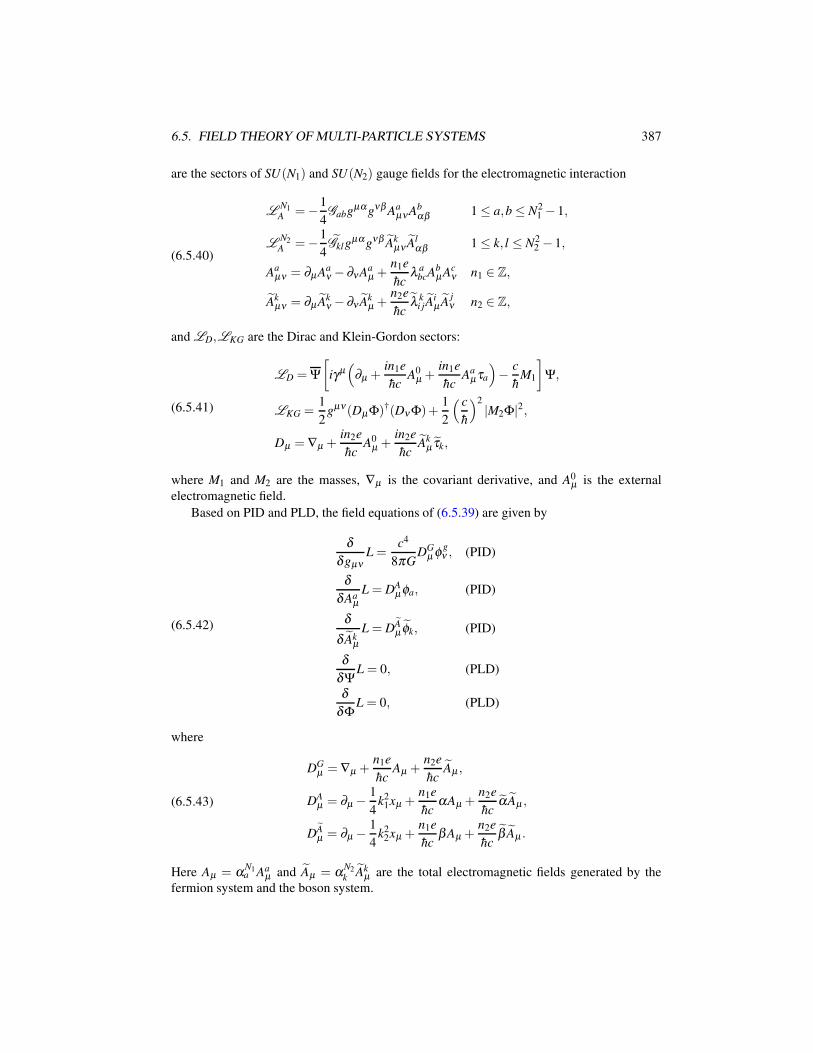
6.5. FIELD THEORY OF MULTI-PARTICLE SYSTEMS 387
are the sectors of SU(N1) and SU(N2) gauge fields for the electromagnetic interaction
(6.5.40)
LN1A =−1
4Gabgµαgνβ Aa
µνAbαβ 1 ≤ a,b ≤ N2
1 − 1,
LN2A =−1
4Gklg
µαgνβ Akµν Al
αβ 1 ≤ k, l ≤ N22 − 1,
Aaµν = ∂µAa
ν − ∂νAaµ +
n1e
hcλ a
bcAbµAc
ν n1 ∈ Z,
Akµν = ∂µ Ak
ν − ∂ν Akµ +
n2e
hcλ k
i jAiµ A
jν n2 ∈ Z,
and LD,LKG are the Dirac and Klein-Gordon sectors:
(6.5.41)
LD = Ψ
[iγµ(
∂µ +in1e
hcA0
µ +in1e
hcAa
µτa
)− c
hM1
]Ψ,
LKG =1
2gµν(DµΦ)†(Dν Φ)+
1
2
( c
h
)2
|M2Φ|2,
Dµ = ∇µ +in2e
hcA0
µ +in2e
hcAk
µ τk,
where M1 and M2 are the masses, ∇µ is the covariant derivative, and A0µ is the external
electromagnetic field.
Based on PID and PLD, the field equations of (6.5.39) are given by
(6.5.42)
δ
δgµνL =
c4
8πGDG
µ φgν , (PID)
δ
δAaµ
L = DAµφa, (PID)
δ
δ Akµ
L = DAµ φk, (PID)
δ
δΨL = 0, (PLD)
δ
δΦL = 0, (PLD)
where
(6.5.43)
DGµ = ∇µ +
n1e
hcAµ +
n2e
hcAµ ,
DAµ = ∂µ −
1
4k2
1xµ +n1e
hcαAµ +
n2e
hcαAµ ,
DAµ = ∂µ −
1
4k2
2xµ +n1e
hcβ Aµ +
n2e
hcβ Aµ .
Here Aµ = αN1a Aa
µ and Aµ = αN2k Ak
µ are the total electromagnetic fields generated by the
fermion system and the boson system.
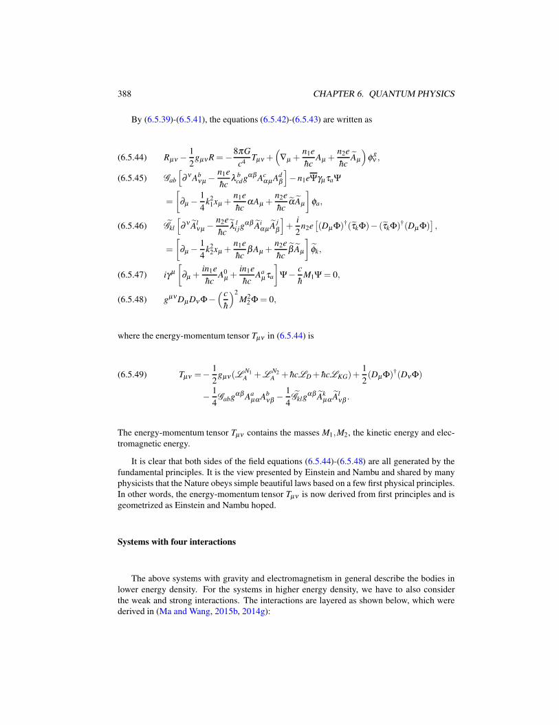
388 CHAPTER 6. QUANTUM PHYSICS
By (6.5.39)-(6.5.41), the equations (6.5.42)-(6.5.43) are written as
Rµν −1
2gµνR =−8πG
c4Tµν +
(∇µ +
n1e
hcAµ +
n2e
hcAµ
)φ
gν ,(6.5.44)
Gab
[∂ ν Ab
νµ −n1e
hcλ b
cdgαβ AcαµAd
β
]− n1eΨγµτaΨ(6.5.45)
=
[∂µ −
1
4k2
1xµ +n1e
hcαAµ +
n2e
hcαAµ
]φa,
Gkl
[∂ ν Al
νµ −n2e
hcλ l
i jgαβ Ai
αµ Aj
β
]+
i
2n2e[(DµΦ)†(τkΦ)− (τkΦ)†(DµΦ)
],(6.5.46)
=
[∂µ −
1
4k2
2xµ +n1e
hcβ Aµ +
n2e
hcβ Aµ
]φk,
iγµ
[∂µ +
in1e
hcA0
µ +in1e
hcAa
µτa
]Ψ− c
hM1Ψ = 0,(6.5.47)
gµνDµDν Φ−(c
h
)2
M22 Φ = 0,(6.5.48)
where the energy-momentum tensor Tµν in (6.5.44) is
Tµν =− 1
2gµν(L
N1A +L
N2A + hcLD + hcLKG)+
1
2(DµΦ)†(DνΦ)(6.5.49)
− 1
4Gabgαβ Aa
µα Abνβ − 1
4Gklg
αβ Akµα Al
νβ .
The energy-momentum tensor Tµν contains the masses M1,M2, the kinetic energy and elec-
tromagnetic energy.
It is clear that both sides of the field equations (6.5.44)-(6.5.48) are all generated by the
fundamental principles. It is the view presented by Einstein and Nambu and shared by many
physicists that the Nature obeys simple beautiful laws based on a few first physical principles.
In other words, the energy-momentum tensor Tµν is now derived from first principles and is
geometrized as Einstein and Nambu hoped.
Systems with four interactions
The above systems with gravity and electromagnetism in general describe the bodies in
lower energy density. For the systems in higher energy density, we have to also consider
the weak and strong interactions. The interactions are layered as shown below, which were
derived in (Ma and Wang, 2015b, 2014g):
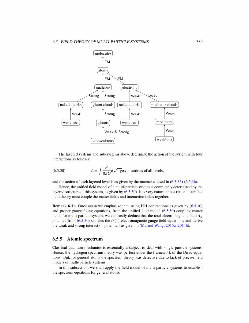
6.5. FIELD THEORY OF MULTI-PARTICLE SYSTEMS 389
molecules
atoms
nucleons electrons
naked quarks gluon clouds
weaktons gluons
w∗-weaktons
naked quarks mediator clouds
weaktons mediators
weaktons
EM
EM EM
Strong Strong
Weak Strong
Weak & Strong
Weak Weak
Weak Weak
Weak
The layered systems and sub-systems above determine the action of the system with four
interactions as follows:
(6.5.50) L =
∫c4
8πGR√−gdx+ actions of all levels,
and the action of each layered level is as given by the manner as used in (6.5.35)-(6.5.36).
Hence, the unified field model of a multi-particle system is completely determined by the
layered structure of this system, as given by (6.5.50). It is very natural that a rationale unified
field theory must couple the matter fields and interaction fields together.
Remark 6.31. Once again we emphasize that, using PRI contractions as given by (6.5.10)
and proper gauge fixing equations, from the unified field model (6.5.50) coupling matter
fields for multi-particle system, we can easily deduce that the total electromagnetic field Aµ
obtained from (6.5.50) satisfies the U(1) electromagnetic gauge field equations, and derive
the weak and strong interaction potentials as given in (Ma and Wang, 2015a, 2014h).
6.5.5 Atomic spectrum
Classical quantum mechanics is essentially a subject to deal with single particle systems.
Hence, the hydrogen spectrum theory was perfect under the framework of the Dirac equa-
tions. But, for general atoms the spectrum theory was defective due to lack of precise field
models of multi-particle systems.
In this subsection, we shall apply the field model of multi-particle systems to establish
the spectrum equations for general atoms.
390 CHAPTER 6. QUANTUM PHYSICS
1. Classical theory of atomic shell structure. We recall that an atom with atomic number
Z has energy spectrum
(6.5.51) En =−Z2
n2
me4
2h2, n = 1,2, · · · .
If we ignore the interactions between electrons, the orbital electrons of this atom have the
idealized discrete energies (6.5.51). The integers n in (6.5.51) are known as principal quantum
number, which characterizes the electron energy levels and orbital shell order:
(6.5.52)n : 1 2 3 4 5 6 7
shell symbol: K L M N O P Q.
Each orbital electron is in some shell of (6.5.52) and possesses the following four quantum
numbers:
1) principle quantum number n = 1,2, · · · ,
2) orbital quantum number l = 0,1,2, · · · ,(n− 1),
3) magnetic quantum number m = 0,±1, · · · ,±l,
4) spin quantum number J =± 12.
For each given shell n, there are sub-shells characterized by orbital quantum number l,
whose symbols are:
(6.5.53)l : 0 1 2 3 4 · · ·sub-shell: s p d f g · · · .
By the Pauli exclusion principle, at a give sub-shell nl, there are at most the following
electron numbers
Nnl = Nl = 2(2l+ 1) for 0 ≤ l ≤ n− 1.
Namely, for the sub-shells s(l = 0), p(l = 1),d(l = 2), f (l = 3),g(l = 4), their maximal elec-
tron numbers are
Ns = 2, Np = 6, Nd = 10, N f = 14, Ng = 18.
Thus, on the n-th shell, the maximal electron number is
(6.5.54) Nn =n−1
∑l=0
Nl = 2n2.
2. Atomic field equations. Based on the atomic shell structure, the electron system of an
atom consists of shell systems as (6.5.52), which we denote by
(6.5.55) Sn = the n-th shell system for n = 1,2, · · · .
Each shell system Sn has n sub-shell systems as in (6.5.53), denoted by
(6.5.56) Snl = the l-th sub-shell system of Sn for 0 ≤ l ≤ n− 1.
6.5. FIELD THEORY OF MULTI-PARTICLE SYSTEMS 391
Thus, we have two kinds of classifications (6.5.55) and (6.5.56) of sub-systems for atomic
orbital electrons, which lead to two different sets of field equations.
A. FIELD EQUATION OF SYSTEM Sn . If we ignore the orbit-orbit interactions, then we
take (6.5.55) as an N-particle system. Let Sn have Kn electrons:
(6.5.57) Sn : Ψn = (ψ1n , · · · ,ψKn
n ), Kn ≤ Nn, 1 ≤ n ≤ N,
where Nn is as in (6.5.54). Hence, the model of (6.5.57) is reduced to the SU(K1)× ·· · ×SU(KN) gauge fields of fermions. Referring to the single fermion system (6.5.15)-(6.5.21),
the action of (6.5.57) is
(6.5.58) L =
∫ N
∑n=1
(LSU(Kn)+LnD)dx,
where
(6.5.59)
LSU(Kn) =− 1
4hcgµαgνβ Aan
µνAan
αβ1 ≤ an ≤ Kn,
LnD = Ψn(iγ
µ Dµ −mec
h)Ψn 1 ≤ n ≤ N,
Aanµν = ∂µAan
ν − ∂νAanµ − e
hcλ an
bncnAbn
µ Acnν ,
DµΨn = (∂µ − ie
hcA0
µ − ie
hcAan
µ τan)Ψn,
where Aanµ are the SU(Kn) gauge fields representing the electromagnetic (EM) potential of
the electrons in Sn, λ an
bncnare the structure constants of SU(Kn) such that Ganbn
= 12tr(τanτ†
bn) =
δanbn, A0
µ is the EM potential generated by the nuclear, g = −e (e > 0) is the charge of an
electron, and me is the electron mass.
The PID gradient operators for SU(K1)×·· ·× SU(KN) in (6.5.19) are given by
(6.5.60) Dnµ =
1
hc
[∂µ +
e
hc∑k 6=n
A(k)µ
]for 1 ≤ n ≤ N,
where A(k)µ = α
KkaK A
akµ is the total EM potential of Sk shell as defined in (6.5.10).
Then by (6.5.58)-(6.5.60), the field equations of (6.5.57) can be written in the following
form
∂ ν Aanνµ +
e
hcλ an
bncngαβ Abn
αµAcn
β + eΨγµτanΨn(6.5.61)
=
[∂µ +
e
hc∑k 6=n
A(k)µ
]φan for 1 ≤ an ≤ K2
n − 1, 1 ≤ n ≤ N,
iγµ
[∂µ − ie
hcA0
µ −ie
hcAan
µ τan
]Ψn −
mec
hΨn = 0.(6.5.62)
392 CHAPTER 6. QUANTUM PHYSICS
B. FIELD EQUATION OF SYSTEM Snl . The precise model of atomic spectrum should take
(6.5.56) as an N-particle system. Also, Sn =n−1
∑l=0
Snl is again divided into n sub-systems
Sn : Sn0, · · · ,Snn−1.
Hence, the system Snl has more sub-systems than Sn, i.e. if Sn has N sub-systems, then Snl
has 12N(N + 1) sub-systems.
Let Snl have Knl electrons with wave functions:
(6.5.63) Snl : Ψnl = (ψ1nl , · · · ,ψ
Knl
nl ), 1 ≤ n ≤ N, 0 ≤ l ≤ n− 1,
and Knl ≤ 2(2l+ 1). Then the action of (6.5.63) takes as
(6.5.64) L =∫ n−1
∑l=0
N
∑n=1
(LSU(Knl )+L
nlD )dx,
where LSU(Knl ) and L nlD are similar to that of (6.5.59). Thus, the field equation of the system
(6.5.63) is determined by (6.5.64).
Remark 6.32. The reason why atomic spectrum can be divided into two systems (6.5.57)
and (6.5.63) to be considered is that in the system (6.5.63) the electrons in each Snl have the
same energy, and in (6.5.57) the electons in each Sn have the same energy if we ignore the
interaction energy between different l-orbital electrons of Snl. Hence, the system of Snl is
precise and the system of Sn is approximative.
3. Atomic spectrum equations. For simplicity, we only consider the system Sn, and for
Snl the case is similar. Since the electrons in each Sn have the same energy λn, the wave
functions in (6.5.57) can take as
(6.5.65) ψ jn = ϕ j
n(x)e−iλnt/h for 1 ≤ j ≤ Kn.
It is known that the EM fields Aaµ in atomic shells are independent of time t, i.e. ∂tA
aµ = 0.
Therefore, inserting (6.5.65) into (6.5.61) and (6.5.62) we derive the spectrum equation in the
form
λnΦn = ich(~α ·D)Φn − eVΦn +mec2α0Φn + eAan0 τan Φn for 1 ≤ n ≤ N,(6.5.66)
∆Aan0 − e
hcλ an
bncn
~Abn · (∇Acn0 +
e
hcλ cn
dn fnAdn~A fn)− eΦ†
nτanΦn =e
hc∑k 6=n
A(k)0 φan ,(6.5.67)
∆~Aan −∇( div ~Aan)+e
hcλ an
bncngαα~Abn
α Acnα + eΦ)n~γτanΦn = (∇+
e
hc∑k 6=n
~A(k))φan ,(6.5.68)
where Φn = (ϕ1n , · · · ,ϕKn
n )T ,Aanµ = (Aan
0 ,~Aan),~α = (α1,α2,α3) and α0 are as in (3.1.15),~γ =
(γ1,γ2,γ3) is as in (6.2.8), V = ze/r is the Coulomb potential of the nuclear, ~A = (A1,A2,A3)is the magnetic potential of the nuclear, and
DΦn = (∇− ie
hc~A− ie
hc~Aanτan)Φn,
~Abnα = ∂α
~Abn −∇Abnα − e
hcλ bn
cndnAcn
α~Adn .

6.5. FIELD THEORY OF MULTI-PARTICLE SYSTEMS 393
The equations (6.5.66)-(6.5.68) need to be complemented with some gauge fixing equa-
tions; see Remark 6.29.

394 CHAPTER 6. QUANTUM PHYSICS
Chapter 7
Astrophysics and Cosmology
The aim of this chapter is to study fundamental issues of astrophysics and cosmology based
on the first principles dictating the law of gravity, the cosmological principle, and the principle
of symmetry-breaking. The study and the results presented in this chapter are based on recent
papers (Ma and Wang, 2014e,a; Hernandez, Ma and Wang, 2015).
First, we have rigorously proved a basic Blackhole Theorem on the nature and structure
of black holes, Theorem 7.15:
Assume the validity of the Einstein theory of general relativity, then black holes
are closed, innate and incompressible.
This theorem was originally discovered and proved in (Ma and Wang, 2014a, Theorem
4.1). One important part of the theorem is that all black holes are closed: matters can neither
enter nor leave their interiors. Classical view was that nothing can get out of black holes, but
matters can fall into blackholes. We show that nothing can get inside the blackhole either.
This theorem offers a very different views on the geometric structure and the origin of our
Universe, on the formation and stability of stars and galaxies, and on the mechanism of
supernovae and active galactic nucleus (AGN) jets.
In particular, we rigorously show that our Universe is not originated from a Big-Bang,
and is static, under the assumption of the Einstein general relativity and the cosmological
principle. The redshift is then due mainly to the black hole effect, and the CMB is caused by
the blackbody equilibrium radiation.
Also, we show that the dark energy is associated with the the negative pressure, the effect
of the gravitational repelling force, and the dark matter is caused the space curved energy.
This chapter is organized as follows. Section 7.1 introduces the momentum representation
of astrophysical fluid dynamical models. One important aspect of the models is the coupling
between the gravitational field equations and the fluid dynamics equations, using the principle
of symmetry-breaking. Section 7.4 proves the black hole theorem.
Stellar circulations are studied in Section 7.2, leading to the mechanism of supernovae
explosion. Section 7.3 addresses galactic circulations, and provides the mechanism of AGN
jets.
395
396 CHAPTER 7. ASTROPHYSICS AND COSMOLOGY
Based on the black hole theorem, theorems on the structure and origin of the Universe are
proved in Section 7.5.
Finally, in Section 7.6, we have derived 1) the PID cosmological model of our Universe,
2) the nature of dark energy and dark matter, and 3) the gravitational force formulas.
7.1 Astrophysical Fluid Dynamics
The main objective of this section is to establish fluid dynamical models for astrophysical and
cosmological objects such as stars, galaxies, and clusters of galaxies, based on the Principle
of Symmetry-Breaking 2.14.
7.1.1 Fluid dynamic equations on Riemannian manifolds
To consider astrophysical fluid dynamics, we first need to discuss the Navier-Stokes equations
on Riemannian manifolds.
Let (M ,gi j) be an n-dimensional Riemannian manifold. The fluid motion on M are
governed by the Navier-Stokes equations given by
(7.1.1)
∂u
∂ t+(u ·∇)u = ν∆u− 1
ρ∇p+ f for x ∈ M ,
divu = 0,
where u = (u1, · · · ,un) is the velocity field, p is the pressure, f is the external force, ρ is
the mass density, ν is the dynamic viscosity, and the differential operator ∆ is the Laplace-
Beltrami operator defined as ∆u = (∆u1, · · · ,∆un) with
∆ui = div(∇ui)+ gi jR jkuk,(7.1.2)
div(∇ui) = gkl
[∂
∂xl
(∂ui
∂xk+Γi
k juj
)+Γi
l j
(∂u j
∂xk+Γ
j
ksus
)(7.1.3)
−Γ jkl
(∂ui
∂x j+Γi
jsus
)].
Here Ri j is the Ricci curvature tensor and Γik j the Levi-Civita connection:
Ri j =1
2gkl
(∂ 2gkl
∂xi∂x j+
∂ 2gi j
∂xk∂xl− ∂ 2gk j
∂xi∂xl− ∂ 2gli
∂x j∂xk
)(7.1.4)
+ gklgrs
(Γr
klΓsi j −Γr
ilΓsk j
),
Γik j =
1
2gil
(∂gkl
∂x j+
∂g jl
∂xk− ∂gk j
∂xl
).(7.1.5)
The nonlinear convection term (u ·∇)u in (7.1.1) is defined by
(7.1.6)
(u ·∇)u = (uiDiu1, · · · ,uiDiu
n),
uiDiuk = ui ∂uk
∂xi+Γk
i juiu j
7.1. ASTROPHYSICAL FLUID DYNAMICS 397
the pressure term is
(7.1.7) ∇p =
(g1k ∂ p
∂xk, · · · ,gnk ∂ p
∂xk
),
the divergence of u is
(7.1.8) divu =∂uk
∂xk+Γk
jku j =1√g
∂ (√
guk)
∂xk,
and g = det(gi j).By (7.1.2) and (7.1.6)-(7.1.8), the Navier-Stokes equations (7.1.1) can be equivalently
written as
(7.1.9)
∂ui
∂ t+ uk ∂ui
∂xk+Γi
k juku j = ν
[div(∇ui)+ gi jR jkuk
]− 1
ρgi j ∂ p
∂x j+ f i,
∂uk
∂xk+Γk
jku j = 0.
Remark 7.1. In the Navier-Stokes equations (7.1.1), the Laplace operator ∆ can be taken in
two forms:
∆ = dδ + δd the Laplace-Beltrami operator,(7.1.10)
∆ = div ·∇ the Laplace operator.(7.1.11)
Here we choose (7.1.10) instead of (7.1.11) to represent the viscous term in (7.1.1). The
reason is that the Laplace-Beltrami operator
(dδ + δd)ui = div ·∇ui + gi jR jkuk
gives rise to an additional term gi jR jkuk. In fluid dynamics, the term µ div ·∇u represents
the viscous (frictional) force, and the term gi jR jkuk is the force generated by space curvature
and gravitational interaction. Hence physically, it is more natural to take (7.1.10) instead of
(7.1.11).
Remark 7.2. In the fluid dynamic equations (7.1.9), the symmetry of general relativity
breaks, and the space and time are treated independently.
7.1.2 Schwarzschild and Tolman-Oppenheimer-Volkoff (TOV) metrics
We recall in this section the classical Schwarzschild and TOV metrics for centrally symmetric
gravitational fields.
Schwarzschild metric
Many stars in the Universe are spherically-shaped, generating centrally symmetric gravi-
tational fields. It is known that the Riemannian metric of a spherically symmetric gravitation
field takes the following form:
(7.1.12) ds2 =−euc2dt2 + evdr2 + r2(dθ 2 + sin2 θdϕ2),
398 CHAPTER 7. ASTROPHYSICS AND COSMOLOGY
where (r,θ ,ϕ) is the spherical coordinate system, and u = u(r, t) and v = v(r, t) are functions
of r and t, which are determined by the gravitational field equations.
In the exterior of a ball, Schwarzschild first obtained an exact solution of the Einstein
field equations in 1916, which describes the gravitational fields for the external vacuum state
of a static spherically symmetric matter field.
Let m be the total mass of a centrally symmetric ball. Then the classical Newtonian
gravitational potential of the ball reads
(7.1.13) ϕ =−mG
r.
Based on the Einstein general theory of relativity, the time-component g00 of gravitational
potential gµν and the Newton potential ϕ have the following relation
(7.1.14) g00 =−(
1+2
c2ϕ
)
Hence, by (7.1.13) and (7.1.14) for the ball we have
(7.1.15) g00 =−1+2mG
c2r.
Now we consider the gravitational field equations in the exterior of the ball. In the vacuum
state,
(7.1.16) Tµν = 0.
On the other hand, by R = gµνRµν , the Einstein gravitational field equations
Rµν −1
2gµνR =−8πG
c4Tµν
can be equivalently written as
Rµν =−8πG
c4(Tµν −
1
2gµνT ), T = gklTkl .
Thus, by (7.1.16) the Einstein field equations become
(7.1.17) Rµν = 0
The nonzero components of the metric (7.1.12) gµν are
(7.1.18) g00 =−eu, g11 = ev, g22 = r2, g33 = r2 sin2 θ .
Since the gravitational resource is static, u and v only depend on r. By (7.1.18), all
nonzero components of the Levi-Civita connection (7.1.5) are given by
(7.1.19)
Γ100 =
1
2eu−vu′, Γ1
11 =1
2v′, Γ1
22 =−re−v,
Γ133 =−re−v sin2 θ , Γ0
10 =1
2u′, Γ2
12 =1
r,
Γ233 =−sinθ cosθ , Γ3
13 =1
r, Γ3
23 =cosθ
sinθ.
7.1. ASTROPHYSICAL FLUID DYNAMICS 399
Thus, by (7.1.4) and (7.1.19) we get Rµν as
(7.1.20)
R00 = eu−v
[−1
2u′′− 1
ru′+
1
ru′(v′− u′)
],
R11 =1
2u′′− 1
rv′− 1
4u′(v′− u′),
R22 = e−v[1− ev+
r
2(u′− v′)
],
R33 = R22 sin2 θ ,
Rµν = 0 ∀µ 6= ν.
Therefore, the vacuum Einstein field equations (7.1.17) become the following system of
ordinary differential equations
1
2u′′+
1
ru′− 1
4(v′− u′)u′ = 0,(7.1.21)
1
2u′′− 1
rv′− 1
4(v′− u′)u′ = 0,(7.1.22)
r
2(u′− v′)− ev + 1 = 0.(7.1.23)
By the Bianchi identity, only two equations of (7.1.22)-(7.1.23) are independent. The
difference of (7.1.21) and (7.1.22) leads to
u′+ v′ = 0,
which implies that
(7.1.24) u+ v = β ( constant),
and (7.1.23) becomes
ev + rv′− 1 = 0.
Namelyd
dr(re−v) = 1.
It follows that
e−v = 1− b
r,
where b is a to-be-determined constant.
Then it follows from (7.1.24) that
eu = eβ e−v = eβ (1− b
r).
By scaling time t, we can take eβ = 1. Hence the solution of the Einstein field equations
(7.1.17) is given by
(7.1.25)
g00 =−eu =−(
1− b
r
),
g11 = ev =
(1− b
r
)−1
.
400 CHAPTER 7. ASTROPHYSICS AND COSMOLOGY
Comparing (7.1.25) with (7.1.15), we can obtain
b =2mG
c2.
Thus, we get the solution of (7.1.17) as
g00 =−(
1− 2mG
c2r
),
g11 =
(1− 2mG
c2r
)−1
,
and the metric reads
(7.1.26) ds2 =−(
1− 2mG
c2r
)c2dt2 +
(1− 2mG
c2r
)−1
dr2 + r2dθ 2 + r2 sin2 θdϕ2,
We have in particular
e−v = eu = 1− 2mG
c2r.
which is called the Schwarzschild solution or metric.
TOV metric
The Schwarzschild metric (7.1.26) describes the exterior gravitational fields of a centrally
symmetric ball. For the interior gravitational fields, the metric is given by the TOV solution.
Let m be the mass of a centrally symmetric ball, and R be the radius of this ball. In the
interior of the ball, the variable r satisfies 0 ≤ r < R. Let the ball be a static liquid sphere
consisting of idealized fluid, an approximation of stars. The energy-momentum tensor of an
idealized fluid is in the form
T µν = (ρ + p)uµuν + pgµν ,
where p is the pressure, ρ is the density, and uµ is the 4-velocity. For a static fluid, uµ is
given by
uµ =1√−g00
(1,0,0,0).
Hence, the (1,1)-type of the energy-momentum tensor is in the form
T νµ =
−c2ρ 0 0 0
0 p 0 0
0 0 p 0
0 0 0 p
.
The Einstein gravitational field equations of an interior ball read
(7.1.27)Rν
µ −1
2δ ν
µ R =−8πG
c4T ν
µ ,
DνT νµ = 0.
7.1. ASTROPHYSICAL FLUID DYNAMICS 401
By (7.1.20) we have
R = gµνRµν =−e−uR00 + e−νR11 +2
r2R22.
Then, by (7.1.20) and Rνµ = gνα Rαµ we get
R00 −
1
2R =−e−v
(1
r2− v′
r
)+
1
r2,
R11 −
1
2R =−e−v
(u′
r+
1
r2
)+
1
r2,
R22 −
1
2R =−1
2e−v
(u′′− 1
2u′v′+
1
2u′2 +
1
ru′− 1
rv′)
In addition, we know that
Dα T αµ = D0T 0
µ +D1T 1µ +D2T 2
µ +D3T 3µ ,
Dα Tβµ =
∂Tβµ
∂xα+Γ
βανT ν
µ −ΓναµT
βν .
Thus, by (7.1.19) we have
Dα T α1 =
d p
dr+
1
2(p+ c2ρ)u′,
Dα T αµ = 0 for µ 6= 1.
Hence, the field equations (7.1.27) can be written as
e−v
(1
r2− v′
r
)− 1
r2=−8πG
c2ρ ,(7.1.28)
e−v
(1
r2+
u′
r
)− 1
r2=
8πG
c4p,(7.1.29)
e−v(u′′− 1
2u′v′+
1
2u′2 +
1
ru′− 1
rv′) =
16πG
c2p,(7.1.30)
p′+1
2(p+ c2ρ)u′ = 0.(7.1.31)
By the Bianchi identity, only three equations of (7.1.28)-(7.1.31) are independent. Here
we also regard p and ρ as unknown functions. Therefore, for the four unknown functions
u,v, p,ρ , we have to add an equation of state to the system of (7.1.28)-(7.1.31):
(7.1.32) ρ = f (p),
and the function f will be given according to physical conditions.
On the surface r = R of the ball, p= 0 and u and v are given in terms of the Schwarzschild
solution:
(7.1.33) p(R) = 0, u(R) =−v(R) = ln
(1− 2Gm
Rc2
).
402 CHAPTER 7. ASTROPHYSICS AND COSMOLOGY
We are now in position to discuss the solutions of problem (7.1.28)-(7.1.33). Let
(7.1.34) M(r) =c2r
2G(1− e−v).
Then the equation (7.1.28) can be rewritten as
1
r2
dM
dr= 4πρ ,
whose solution is given by
(7.1.35) M(r) =
∫ r
04πr2ρdr for 0 < r < R.
By (7.1.35), we see that M(r) is the mass, contained in the ball Br. It follows from (7.1.34)
that
(7.1.36) e−v = 1− 2GM(r)
c2r.
Inserting (7.1.36) in (7.1.29) we obtain
(7.1.37) u′ =1
r(c2r− 2MG)
[8πG
c2pr3 + 2GM(r)
].
Putting (7.1.37) into (7.1.31) we get
(7.1.38) p′ =− (p+ c2ρ)
2r(c2r− 2MG)
[8πG
c2pr3 + 2GM(r)
].
Thus, it suffices for us to derive the solution p,M and ρ from (7.1.32)-(7.1.34) and
(7.1.38), and then v and u will follow from (7.1.36)-(7.1.37) and (7.1.33).
The equation (7.1.38) is called the TOV equation, which was derived to describe the
structure of neutron stars.
We note that (7.1.36) is the interior metric of a blackhole provided that 2GM(r)/c2r =1. Thus the TOV solution (7.1.36) gives a rigorous proof of the following theorem for the
existence of black holes.
Theorem 7.3. If the matter field in a ball BR of radius R is spherically symmetric, and the
mass MR and the radius R satisfy
2GMR
c2R= 1,
then the ball must be a blackhole.
An idealized model is that the density is homogeneous, i.e. (7.1.32) is given by
ρ = ρ0 a constant.
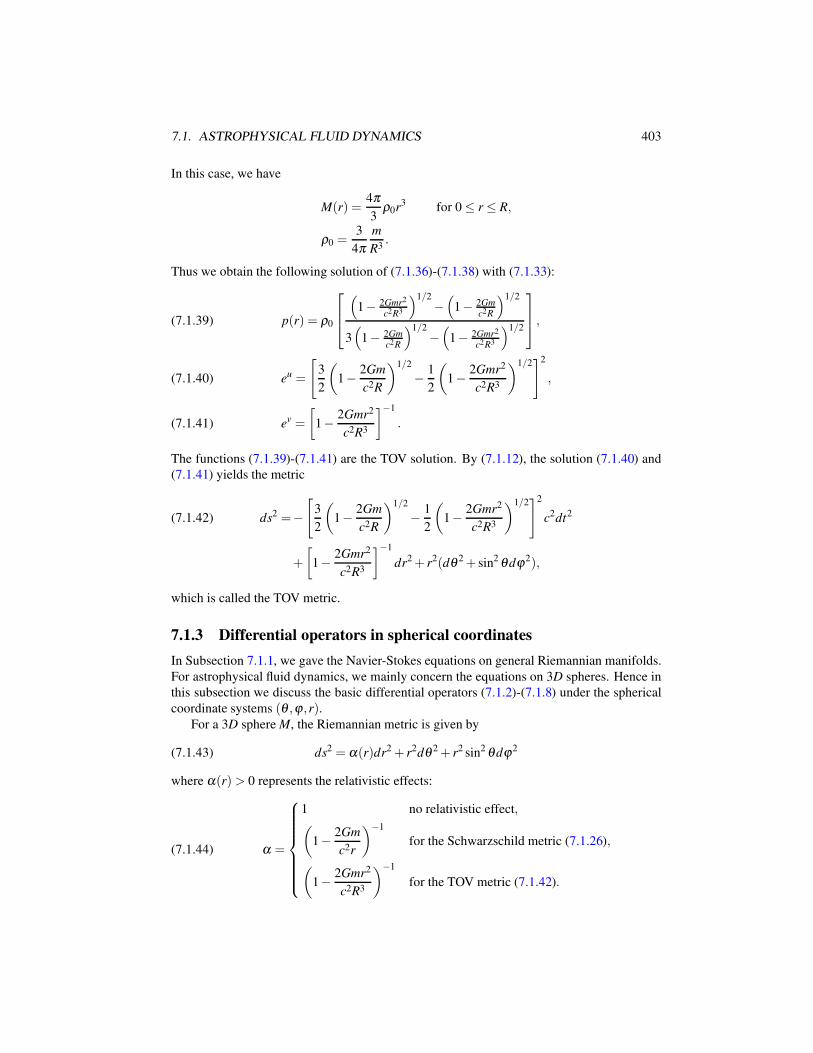
7.1. ASTROPHYSICAL FLUID DYNAMICS 403
In this case, we have
M(r) =4π
3ρ0r3 for 0 ≤ r ≤ R,
ρ0 =3
4π
m
R3.
Thus we obtain the following solution of (7.1.36)-(7.1.38) with (7.1.33):
p(r) = ρ0
(1− 2Gmr2
c2R3
)1/2
−(
1− 2Gmc2R
)1/2
3(
1− 2Gmc2R
)1/2
−(
1− 2Gmr2
c2R3
)1/2
,(7.1.39)
eu =
[3
2
(1− 2Gm
c2R
)1/2
− 1
2
(1− 2Gmr2
c2R3
)1/2]2
,(7.1.40)
ev =
[1− 2Gmr2
c2R3
]−1
.(7.1.41)
The functions (7.1.39)-(7.1.41) are the TOV solution. By (7.1.12), the solution (7.1.40) and
(7.1.41) yields the metric
ds2 =−[
3
2
(1− 2Gm
c2R
)1/2
− 1
2
(1− 2Gmr2
c2R3
)1/2]2
c2dt2(7.1.42)
+
[1− 2Gmr2
c2R3
]−1
dr2 + r2(dθ 2 + sin2 θdϕ2),
which is called the TOV metric.
7.1.3 Differential operators in spherical coordinates
In Subsection 7.1.1, we gave the Navier-Stokes equations on general Riemannian manifolds.
For astrophysical fluid dynamics, we mainly concern the equations on 3D spheres. Hence in
this subsection we discuss the basic differential operators (7.1.2)-(7.1.8) under the spherical
coordinate systems (θ ,ϕ ,r).For a 3D sphere M, the Riemannian metric is given by
(7.1.43) ds2 = α(r)dr2 + r2dθ 2 + r2 sin2 θdϕ2
where α(r)> 0 represents the relativistic effects:
(7.1.44) α =
1 no relativistic effect,(
1− 2Gm
c2r
)−1
for the Schwarzschild metric (7.1.26),
(1− 2Gmr2
c2R3
)−1
for the TOV metric (7.1.42).
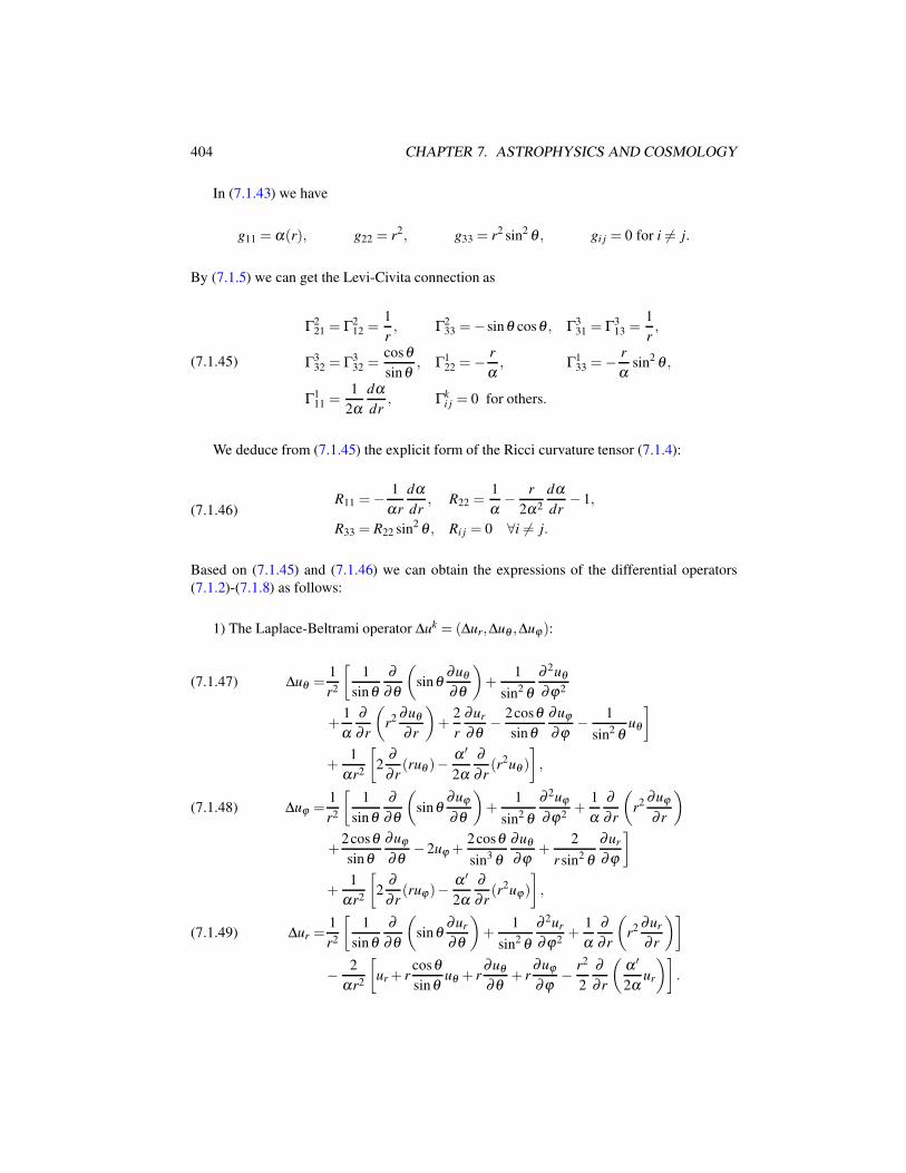
404 CHAPTER 7. ASTROPHYSICS AND COSMOLOGY
In (7.1.43) we have
g11 = α(r), g22 = r2, g33 = r2 sin2 θ , gi j = 0 for i 6= j.
By (7.1.5) we can get the Levi-Civita connection as
(7.1.45)
Γ221 = Γ2
12 =1
r, Γ2
33 =−sinθ cosθ , Γ331 = Γ3
13 =1
r,
Γ332 = Γ3
32 =cosθ
sinθ, Γ1
22 =− r
α, Γ1
33 =− r
αsin2 θ ,
Γ111 =
1
2α
dα
dr, Γk
i j = 0 for others.
We deduce from (7.1.45) the explicit form of the Ricci curvature tensor (7.1.4):
(7.1.46)R11 =− 1
αr
dα
dr, R22 =
1
α− r
2α2
dα
dr− 1,
R33 = R22 sin2 θ , Ri j = 0 ∀i 6= j.
Based on (7.1.45) and (7.1.46) we can obtain the expressions of the differential operators
(7.1.2)-(7.1.8) as follows:
1) The Laplace-Beltrami operator ∆uk = (∆ur,∆uθ ,∆uϕ):
∆uθ =1
r2
[1
sinθ
∂
∂θ
(sinθ
∂uθ
∂θ
)+
1
sin2 θ
∂ 2uθ
∂ϕ2(7.1.47)
+1
α
∂
∂ r
(r2 ∂uθ
∂ r
)+
2
r
∂ur
∂θ− 2cosθ
sinθ
∂uϕ
∂ϕ− 1
sin2 θuθ
]
+1
αr2
[2
∂
∂ r(ruθ )−
α ′
2α
∂
∂ r(r2uθ )
],
∆uϕ =1
r2
[1
sinθ
∂
∂θ
(sinθ
∂uϕ
∂θ
)+
1
sin2 θ
∂ 2uϕ
∂ϕ2+
1
α
∂
∂ r
(r2 ∂uϕ
∂ r
)(7.1.48)
+2cosθ
sinθ
∂uϕ
∂θ− 2uϕ +
2cosθ
sin3 θ
∂uθ
∂ϕ+
2
r sin2 θ
∂ur
∂ϕ
]
+1
αr2
[2
∂
∂ r(ruϕ)−
α ′
2α
∂
∂ r(r2uϕ)
],
∆ur =1
r2
[1
sinθ
∂
∂θ
(sinθ
∂ur
∂θ
)+
1
sin2 θ
∂ 2ur
∂ϕ2+
1
α
∂
∂ r
(r2 ∂ur
∂ r
)](7.1.49)
− 2
αr2
[ur + r
cosθ
sinθuθ + r
∂uθ
∂θ+ r
∂uϕ
∂ϕ− r2
2
∂
∂ r
(α ′
2αur
)].
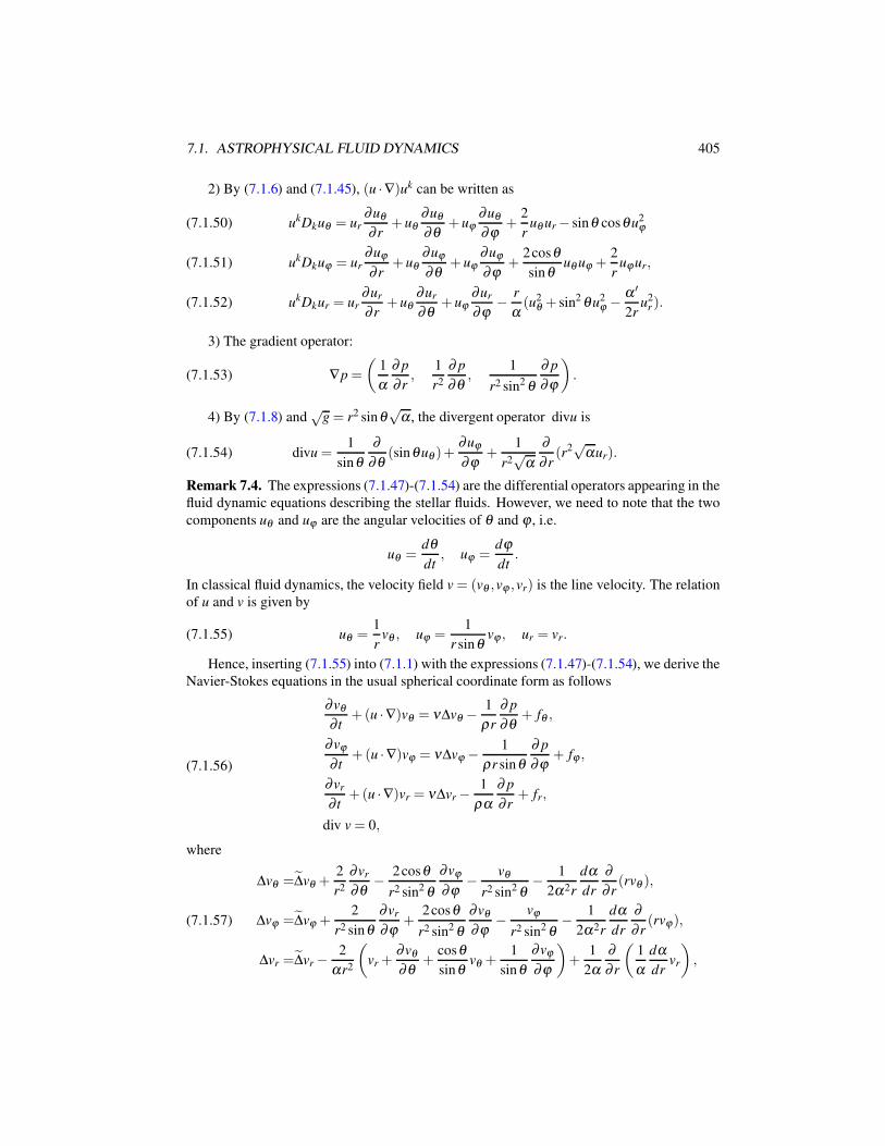
7.1. ASTROPHYSICAL FLUID DYNAMICS 405
2) By (7.1.6) and (7.1.45), (u ·∇)uk can be written as
ukDkuθ = ur∂uθ
∂ r+ uθ
∂uθ
∂θ+ uϕ
∂uθ
∂ϕ+
2
ruθ ur − sinθ cosθu2
ϕ(7.1.50)
ukDkuϕ = ur
∂uϕ
∂ r+ uθ
∂uϕ
∂θ+ uϕ
∂uϕ
∂ϕ+
2cosθ
sinθuθ uϕ +
2
ruϕur,(7.1.51)
ukDkur = ur∂ur
∂ r+ uθ
∂ur
∂θ+ uϕ
∂ur
∂ϕ− r
α(u2
θ + sin2 θu2ϕ − α ′
2ru2
r ).(7.1.52)
3) The gradient operator:
(7.1.53) ∇p =
(1
α
∂ p
∂ r,
1
r2
∂ p
∂θ,
1
r2 sin2 θ
∂ p
∂ϕ
).
4) By (7.1.8) and√
g = r2 sinθ√
α , the divergent operator divu is
(7.1.54) divu =1
sinθ
∂
∂θ(sinθuθ )+
∂uϕ
∂ϕ+
1
r2√
α
∂
∂ r(r2
√αur).
Remark 7.4. The expressions (7.1.47)-(7.1.54) are the differential operators appearing in the
fluid dynamic equations describing the stellar fluids. However, we need to note that the two
components uθ and uϕ are the angular velocities of θ and ϕ , i.e.
uθ =dθ
dt, uϕ =
dϕ
dt.
In classical fluid dynamics, the velocity field v = (vθ ,vϕ ,vr) is the line velocity. The relation
of u and v is given by
(7.1.55) uθ =1
rvθ , uϕ =
1
r sinθvϕ , ur = vr.
Hence, inserting (7.1.55) into (7.1.1) with the expressions (7.1.47)-(7.1.54), we derive the
Navier-Stokes equations in the usual spherical coordinate form as follows
(7.1.56)
∂vθ
∂ t+(u ·∇)vθ = ν∆vθ −
1
ρr
∂ p
∂θ+ fθ ,
∂vϕ
∂ t+(u ·∇)vϕ = ν∆vϕ − 1
ρr sinθ
∂ p
∂ϕ+ fϕ ,
∂vr
∂ t+(u ·∇)vr = ν∆vr −
1
ρα
∂ p
∂ r+ fr,
div v = 0,
where
(7.1.57)
∆vθ =∆vθ +2
r2
∂vr
∂θ− 2cosθ
r2 sin2 θ
∂vϕ
∂ϕ− vθ
r2 sin2 θ− 1
2α2r
dα
dr
∂
∂ r(rvθ ),
∆vϕ =∆vϕ +2
r2 sinθ
∂vr
∂ϕ+
2cosθ
r2 sin2 θ
∂vθ
∂ϕ− vϕ
r2 sin2 θ− 1
2α2r
dα
dr
∂
∂ r(rvϕ),
∆vr =∆vr −2
αr2
(vr +
∂vθ
∂θ+
cosθ
sinθvθ +
1
sinθ
∂vϕ
∂ϕ
)+
1
2α
∂
∂ r
(1
α
dα
drvr
),
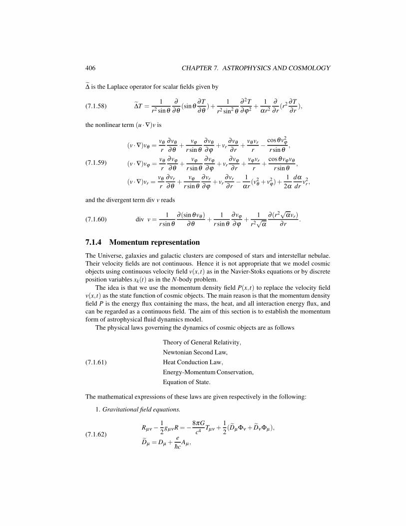
406 CHAPTER 7. ASTROPHYSICS AND COSMOLOGY
∆ is the Laplace operator for scalar fields given by
(7.1.58) ∆T =1
r2 sinθ
∂
∂θ(sinθ
∂T
∂θ)+
1
r2 sin2 θ
∂ 2T
∂ϕ2+
1
αr2
∂
∂ r(r2 ∂T
∂ r),
the nonlinear term (u ·∇)v is
(7.1.59)
(v ·∇)vθ =vθ
r
∂vθ
∂θ+
vϕ
r sin θ
∂vθ
∂ϕ+ vr
∂vθ
∂ r+
vθ vr
r−
cosθv2ϕ
r sin θ,
(v ·∇)vϕ =vθ
r
∂vϕ
∂θ+
vϕ
r sin θ
∂vϕ
∂ϕ+ vr
∂vϕ
∂ r+
vϕvr
r+
cosθvϕvθ
r sinθ,
(v ·∇)vr =vθ
r
∂vr
∂θ+
vϕ
r sinθ
∂vr
∂ϕ+ vr
∂vr
∂ r− 1
αr(v2
θ + v2ϕ)+
1
2α
dα
drv2
r ,
and the divergent term div v reads
(7.1.60) div v =1
r sinθ
∂ (sin θvθ )
∂θ+
1
r sin θ
∂vϕ
∂ϕ+
1
r2√
α
∂ (r2√
αvr)
∂ r.
7.1.4 Momentum representation
The Universe, galaxies and galactic clusters are composed of stars and interstellar nebulae.
Their velocity fields are not continuous. Hence it is not appropriate that we model cosmic
objects using continuous velocity field v(x, t) as in the Navier-Stoks equations or by discrete
position variables xk(t) as in the N-body problem.
The idea is that we use the momentum density field P(x, t) to replace the velocity field
v(x, t) as the state function of cosmic objects. The main reason is that the momentum density
field P is the energy flux containing the mass, the heat, and all interaction energy flux, and
can be regarded as a continuous field. The aim of this section is to establish the momentum
form of astrophysical fluid dynamics model.
The physical laws governing the dynamics of cosmic objects are as follows
(7.1.61)
Theory of General Relativity,
Newtonian Second Law,
Heat Conduction Law,
Energy-Momentum Conservation,
Equation of State.
The mathematical expressions of these laws are given respectively in the following:
1. Gravitational field equations.
(7.1.62)Rµν −
1
2gµνR =−8πG
c4Tµν +
1
2(Dµ Φν + DνΦµ),
Dµ = Dµ +e
hcAµ ,
7.1. ASTROPHYSICAL FLUID DYNAMICS 407
where Aµ is the electromagnetic potential, the time components of gµν are as
g00 =−(
1+2
c2ψ
), g0k = gk0 = 0 for 1 ≤ k ≤ 3,
and ψ is the gravitational potential.
2. Fluid dynamic equations. The Newton Second Law can be expressed as
(7.1.63)dP
dτ= Force,
where τ is the proper time given by
(7.1.64) dτ =√−g00dt,
P is the momentum density field, formally defined by
dx
dτ=
1
ρP,
with ρ being the energy density,
dP
dτ=
∂P
∂τ+
∂P
∂xk
dxk
dτ=
∂P
∂τ+
1
ρ(P ·∇)P,
and
ν∆P+ µ∇(divP) the frictional force,
−∇p the pressure gradient,
c2
2ρ(1−β T)∇g00 =−ρ(1−β T)∇ψ the gravitational force.
Hence, the momentum form of the fluid dynamic equations (7.1.63) is written as
(7.1.65)∂P
∂τ+
1
ρ(P ·∇)P = ν∆P+ µ∇(divP)−∇p−ρ(1−β T)∇ψ ,
where the differential operators ∆,∇ and (P ·∇) are with respect to the space metric gi j (1 ≤i, j ≤ 3) determined by (7.1.62), as defined in (7.1.2)-(7.1.8).
3. Heat conduction equation:
(7.1.66)∂T
∂τ+
1
ρ(P ·∇)T = κ∆T +Q,
where ∆ is defined as
∆T =− 1√g
∂
∂xi(√
ggi j ∂T
∂x j),
and g = det(gi j),1 ≤ i, j ≤ 3.
4. Energy-momentum conservation:
(7.1.67)∂ρ
∂τ+ divP = 0,
where ρ is the energy density:
408 CHAPTER 7. ASTROPHYSICS AND COSMOLOGY
ρ= mass + electromagnetism + potential + heat.
5. Equation of state:
(7.1.68) p = f (ρ ,T ).
Remark 7.5. Both physical laws (7.1.63) and (7.1.67) are the more general form than the
classical ones:
(7.1.69)
mdv
dτ= Force the Newton Second Law,
∂m
∂τ+ div(mv) = 0 the continuity equation,
where m is the mass density. Hence the momentum representation equations (7.1.65)-(7.1.67)
can be applicable in general. The momentum P represents the energy density flux, consisting
essentially of
P = mv+ radiation flux+heat flux.
Hence in astrophysics, the momentum density P is a better candidate than the velocity field
v, to serve as the continuous-media type of state function.
7.1.5 Astrophysical Fluid Dynamics Equations
Dynamic equations of stellar atmosphere
Different from planets, stars are fluid spheres. Like the Sun, most of stars possess at-
mospheric layers. The atmospheric dynamics of stars is an important topic, and we are now
ready to present the stellar atmospheric model.
The spatial domain is a spherical shell:
M = x ∈ R3 | r0 < r < r1.
The stellar atmosphere consists of rarefied gas. For example, the solar corona has mass
density about ρm = 10−9ρ0 where ρ0 is the density of the earth atmosphere. Hence we use
the Schwarzschild solution in (7.1.44) as the metric:
(7.1.70) α(r) =
(1− 2mG
c2r
)−1
, r0 >2mG
c2.
where m is the total mass of the star, and the condition r0 > 2mG/c2 ensures that the star is
not a black hole.
The stellar atmospheric model is the momentum form of the astrophysical fluid dynamical
equations defined on the spherical shell M :
(7.1.71)
∂P
∂τ+
1
ρ(P ·∇)P = ν∆P+ µ∇(divP)−∇p− mGρ
r2(1−β T)~k,
∂T
∂τ+
1
ρ(P ·∇)T = κ∆T,
∂ρ
∂τ+ divP = 0,
7.1. ASTROPHYSICAL FLUID DYNAMICS 409
where P = (Pr,Pθ ,Pϕ) is the momentum density field, T is the temperature, p is the pressure,
ρ is the energy density, ν and µ is the viscosity coefficient, β is the coefficient of thermal
expansion, κ is the thermal diffusivity, α is as in (7.1.70), ∆P,(P ·∇)P, ∆T,div P are as in
(7.1.57)-(7.1.60), and
(7.1.72) (P ·∇)T =Pθ
r
∂T
∂θ+
Pϕ
r sin θ
∂T
∂ϕ+Pr
∂T
∂ r.
The equations (7.1.71) are supplemented with the boundary conditions:
(7.1.73)
Pr = 0,∂Pθ
∂ r= 0,
∂Pϕ
∂ r= 0 at r = r0,r1,
T = T0 at r = r0,
T = T1 at r = r1,
where T0 and T1 are approximatively taken as constants and satisfy the physical condition
T0 > T1.
A few remarks are now in order:
Remark 7.6. First, there are three important parameters: the Rayleigh number Re, the
Prandtl number Pr and the δ -factor δ , which play an important role in astrophysical fluid
dynamics:
(7.1.74) Re =mGr0r1β
κν
T0 −T1
h, Pr =
ν
κ, δ =
2mG
c2r0
.
The δ -factor δ reflects the relativistic effect contained the Laplacian operator.
Remark 7.7. Astronomic observations show that the Sun has three layers of atmospheres:
the photosphere, the chromosphere, and the solar corona, where the solar atmospheric con-
vections occur. It manifests that the thermal convection is a universal phenomenon for stellar
atmospheres. In the classical fluid dynamics, the Rayleigh number dictates the Rayleign-
Benard convection. Here, however, both the Rayleigh number Re and the δ -factor defined by
(7.1.74) play an important role in stellar atmospheric convections.
Remark 7.8. For rotating stars with angular velocity ~Ω, we need add to the right hand side
of (7.1.71) the Coriolis term:
−2~Ω×P = 2Ω(sinθPr − cosθPθ ,cosθPϕ ,−sinθPϕ),
where Ω is the magnitude of ~Ω.
Fluid dynamical equations inside open balls
As the fluid density in a stellar atmosphere is small, the equations (7.1.71) can be regarded
as a precise model governing the stellar atmospheric motion. However, for a fluid sphere with
high density, the fluid dynamic equations have to couple the gravitational field equations.
410 CHAPTER 7. ASTROPHYSICS AND COSMOLOGY
The Universe and all stars are in the momentum-flow state, i.e. they are fluid spheres.
To investigate the interiors of the Universe, galaxies and stars, we need to develop dynamic
models for fluid spheres.
The precise equations of fluid sphere should be defined in the Riemannian metric space
as follows:
(7.1.75) ds2 = g00(x, t)c2dt2 + gi j(x, t)dxidx j for x ∈ M
3,
where M 3 is the spherical space. The gravitational field equations are expressed as
Rµν −1
2gµνR =−8πG
c4Tµν −DµΦµ , (g j0 = g0 j = 0,1 ≤ j ≤ 3),(7.1.76)
where
Tµν = gµα gνβ
[εα εβ + pgαβ
],
and εµ is the 4D energy-momentum vector.
For the fluid component of the system, it is necessary to simplify the model by making
some physically sound approximations.
Approximation Hypothesis 7.9. The metric (7.1.75) and the stationary solutions of the fluid
dynamical equations are radially symmetric.
Under Hypothesis 7.9, the metric (7.1.75) is as in (7.1.12), or is written in the following
form
(7.1.77) ds2 =−ψ(r)c2dt2 +α(r)dr2 + r2dθ 2 + r2 sin2 θdϕ2,
and the fluid dynamic equations are rewritten as
(7.1.78)
∂P
∂τ+
1
ρ(P ·∇)P = ν∆P+ µ∇(divP)−∇p− c2ρ
2α
dψ
dr(1−β (T −T0))~k,
∂T
∂τ+
1
ρ(P ·∇)T = κ∆T +Q(r),
∂ρ
∂τ+ divP = 0,
where P = (Pr,Pθ ,Pϕ),∇P, ∆T,(P ·∇)P, div P are as in (7.1.57)-(7.1.60), ∇p is as in (7.1.56),~k = (1,0,0), and
(P ·∇)T = Pr∂T
∂ r+
Pθ
r
∂T
∂θ+
Pϕ
r sinθ
∂T
∂ϕ.
The gravitational field equation (7.1.76) for the metric (7.1.77) is radially symmetric,
therefore
Φν = Dνφ , φ = φ(r).
Thus we have
D0D0φ =1
2αψψ ′φ ′, D1D1φ =
1
αφ ′′− 1
2α2α ′φ ′,
D2D2φ = D3D3φ =1
rαφ ′, DµDνφ = 0 for µ 6= ν.
7.1. ASTROPHYSICAL FLUID DYNAMICS 411
Then, in view of (7.1.28)-(7.1.31), the equation (7.1.76) can be expressed by
(7.1.79)
1
α
(1
r2− α ′
rα
)− 1
r2=−8πG
c2ρ0 +
1
2αψψ ′φ ′,
1
α
(1
r2+
ψ ′
rψ
)− 1
r2=
8πG
c2p+
1
αφ ′′− 1
2α2α ′φ ′,
1
α
[ψ ′′
ψ− 1
2
(ψ ′
ψ
)2
− α ′ψ ′
2αψ+
1
r
(ψ ′
ψ− α ′
α
)]=
16πG
c2p+
2
rαφ ′,
where the pressure p satisfies the stationary equations of (7.1.78) with P = 0 as follows
(7.1.80)
p′ =−c2
2ψ ′ρ [1−β (T −T0)] ,
κ
αr2
d
dr
(r2 dT
dr
)=−Q(r).
The functions ψ and α satisfy the boundary conditions (7.1.33), i.e.
(7.1.81) ψ(r0) = 1− 2Gm
c2r0
, α(r0) =
(1− 2Gm
c2r0
)−1
.
In addition, for the ordinary differential equations (7.1.79)-(7.1.81), we also need the bound-
ary conditions for ψ ′,φ ′ and T . Since− 12c2ψ ′ represents the gravitational force, the condition
of ψ ′ at r = r0 is given by
(7.1.82) ψ ′(r0) =2mG
c2r20
.
Based on the Newton gravitational law, φ ′ is very small in the external sphere; also see
(Ma and Wang, 2014e). Hence we can approximatively take that
(7.1.83) φ ′(r0) = 0.
Finally, it is rational to take the temperature gradient in the boundary condition as follows
(7.1.84)∂T
∂ r(r0) =−A (A > 0).
Let the stationary solution of the problem (7.1.79)-(7.1.81) be given by p, T ,ψ ,α,φ ′.Make the translation transformation
P → P, p → p+ p, T → T + T .
Then equations (7.1.78) are rewritten in the form
(7.1.85)
∂P
∂τ+
1
ρ(P ·∇)P = ν∆P−∇p+
c2ρ
2α
dψ
drβ~kT,
∂T
∂τ+
1
ρ(P ·∇)T = κ∆T − 1
ρ
dT
drPr,
div P = 0,
412 CHAPTER 7. ASTROPHYSICS AND COSMOLOGY
supplemented with the boundary conditions:
(7.1.86)∂T
∂ r= 0, Pr = 0,
∂Pθ
∂ r=
∂Pϕ
∂ r= 0 at r = r0.
The model (7.1.85)-(7.1.86), we just derived describes interior dynamics of the Universe,
galaxies and stars.
7.2 Stars
7.2.1 Basic knowledge
The large scale structure of the Universe consists of mainly the following levers:
stars, stellar clusters, galaxies, clusters of galaxies.
Star is the most elementary constituent of the Universe, and we now explore some of their
basic properties.
1. Mass m. The mass of the Sun is m⊙ = 2× 1030kg, and the range of the masses of the
main-sequence stars is about
0.1m⊙ ∼ 40m⊙.
A few extreme stars have masses m ≃ 60m⊙, and the least massive stars have masses around
m ≃ 0.07m⊙.
2. Radius R. The radius of the Sun is R⊙ = 7×10⁵km, and the radii of the main-sequence
stars are
0.3R⊙ ∼ 25R⊙.
A neutron star has radius R ≃ 10km, and a red giant star has R = 103R⊙.
3. Surface temperature T . The surface temperature of the Sun is T⊙ = 5800K, and the
range of surface temperatures of stars in general is
2600K ∼ 35000K.
4. Luminosity L. The Sun’s luminosity is L⊙ = 1(4× 1033erg/s), and the luminosities of
the main-sequence stars have ranges in
8× 10⁻³L⊙ ∼ 3.2× 10⁵L⊙.
5. Parameter relation. Based on the radiation theory of black bodies, the above three
parameters R,T,L enjoy
(7.2.1) L = 4πσR2T 4,
where σ is the Stefan-Boltzmann constant:
σ = 5.7× 10⁻⁵erg/cm2 · s ·k4.
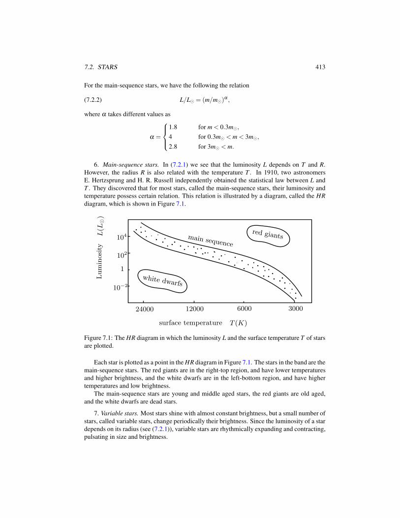
7.2. STARS 413
For the main-sequence stars, we have the following the relation
(7.2.2) L/L⊙ = (m/m⊙)α ,
where α takes different values as
α =
1.8 for m < 0.3m⊙,
4 for 0.3m⊙ < m < 3m⊙,
2.8 for 3m⊙ < m.
6. Main-sequence stars. In (7.2.1) we see that the luminosity L depends on T and R.
However, the radius R is also related with the temperature T . In 1910, two astronomers
E. Hertzsprung and H. R. Russell independently obtained the statistical law between L and
T . They discovered that for most stars, called the main-sequence stars, their luminosity and
temperature possess certain relation. This relation is illustrated by a diagram, called the HR
diagram, which is shown in Figure 7.1.
24000 12000 6000 3000
1white dwarfs
10−2
102
104red giants
Luminosity
L(L
⊙)
surface temperature T (K)
main sequence
Figure 7.1: The HR diagram in which the luminosity L and the surface temperature T of stars
are plotted.
Each star is plotted as a point in the HR diagram in Figure 7.1. The stars in the band are the
main-sequence stars. The red giants are in the right-top region, and have lower temperatures
and higher brightness, and the white dwarfs are in the left-bottom region, and have higher
temperatures and low brightness.
The main-sequence stars are young and middle aged stars, the red giants are old aged,
and the white dwarfs are dead stars.
7. Variable stars. Most stars shine with almost constant brightness, but a small number of
stars, called variable stars, change periodically their brightness. Since the luminosity of a star
depends on its radius (see (7.2.1)), variable stars are rhythmically expanding and contracting,
pulsating in size and brightness.
414 CHAPTER 7. ASTROPHYSICS AND COSMOLOGY
8. Red giants. Stars are held together by gravity. The gravitational force pulling inward
is opposed by a force pushing outward, consisting mainly the thermal pressure in the interior.
Stars maintain their balance of pressure and gravity by the heat energy produced by burning
hydrogen.
Stars less massive than the Sun evolve more slowly and stay on the main-sequence longer
than 1010 years. But more massive stars evolve more quickly, and end their life becoming
white dwarfs and neutron stars (or possibly black holes) as their final fate determined by their
masses.
After a more massive star consumes its central supply of hydrogen, it leaves the main
sequence and enters into the group of red giants in the HR diagram.
When the central nuclear reaction has ceased to generate heat, the interior pressure re-
duces and the star begins to contract, leading to the release of gravitational energy. Hence,
this contraction causes the temperature to rise. Thus, the hydrogen outside the core begins to
burn. The burning shell causes the star to expend. Thus, the star is luminous, large and cool,
and becomes a red giant.
9. White dwarfs. For a star with mass in the range
(7.2.3) 1m⊙ ≤ m < 5m⊙,
when it is in the red-giant phase, its expanding shell is thrown off into space, and the naked
core is all that remains. Contraction ceases, nuclear burning ends, and the core cools down as
a white dwarf. A white dwarf has a size approximatively equal to that of the earth, with mass
m ≤ 1.44M⊙.
10. Neutron stars and pulsars. A star with mass
(7.2.4) 5m⊙ < m,
will eventually evolve to a neutron star. A neutron star has a radius of about 10km with mass
m > 3m⊙, and has a high density of nearly 109ton/cm3. The neutron star has a magnetic field
of 1012 gauss that is 1012 times stronger than the earth’s magnetic field.
The pulsar is a special neutron star, which emits a pulse-like energy message.
11. Supernovae. When a large massive red giant (m > 5m⊙) exhausts its nuclear fuels, it
begins to collapse. This contraction will lead to explosion, and the explosive star is called a
supernova. A neutron star is born after a huge explosion of a supernova.
7.2.2 Main driving force for stellar dynamics
Stars can be regarded as fluid balls. To investigate the stellar interior dynamic behavior, we
need to use the fluid spherical models coupling the heat conductivity equation. There are
two types of starts: stable and unstable. The sizes of stable stars do not change. The main-
sequence stars, white dwarfs and neutron stars are stable stars. The radii of unstable stars may
change; variable stars and expanding red giants are unstable stars. The dynamic equations
governing the two types of stars are different, and will be addressed hereafter separately.
We note that the fluid dynamic equations (7.1.78) represent the Newton’s second law, and
their left-hand sides are the acceleration and their right-hand sides are the total force. The
7.2. STARS 415
total force consists of four parts: the viscous friction, the pressure gradient, the relativistic
effect, and the thermal expansion force, which are given as follows:
• The viscous friction force is caused by the electromagnetic, the weak and the strong
interactions between the particles and the pressure, and is given by
(7.2.5) FνP = νP = ν(∆Pθ ,∆Pϕ ,∆Pr),
as defined by (7.1.57).
• The pressure gradient is defined by:
(7.2.6) −∇p =−(
1
r
∂ p
∂θ,
1
r sinθ
∂ p
∂ϕ,
1
α
∂ p
∂ r
).
• The relativistic effect is reflected in the following terms:
(7.2.7) FGP =
(− ν
2α2r
dα
dr
∂
∂ r(rPθ ),−
ν
2α2r
dα
dr
∂
∂ r(rPϕ),
ν
2α
∂
∂ r
(1
α
dα
drPr
)),
which can be regarded as the coupling interaction between the gravitational potential αand the electromagnetic, the weak and the strong potentials represented by the viscous
coefficient ν .
We shall see that the force (7.2.7) is responsible to the supernova’s huge explosion.
• The thermal expansion force is due to the coupling between the gravity ∇ψ and the
heat Q:
(7.2.8) FT =
(0,0,
c2
2α
dψ
drβ T
),
which is the main driving force for generating stellar interior circulations and nebular
matter spurts of red giants.
The two forces (7.2.7) and (7.2.8) are the main driving forces for the stellar motion, and
hereafter we derive their explicit formulas.
1. Formula for thermal expansion force. The thermal expansion force (7.2.8) is radially
symmetric, which is simply written in the r-component form
fT =c2
2α
dψ
drβ T.
In its nondimensional form, fT is expressed as
(7.2.9) fT = σ(r)T,
and σ(r) is called the thermal factor given by
(7.2.10) σ(r) =−c2r40β
2κ2
1
α
dT
dr
dψ
dr.
416 CHAPTER 7. ASTROPHYSICS AND COSMOLOGY
Here α,ψ ,T satisfy equations (7.1.79)-(7.1.80) with the boundary conditions (7.1.81)-(7.1.84).
The detailed derivation of (7.2.9)-(7.2.10) will be given hereafter.
The σ -factor (7.2.10) can be expressed in the following form, to be deduced later:
σ(r) =c2r3
0(1− δ )β
2κ2r2
eζ (r)
eζ (1)· (1− δ r2 −η) ·
(1
r2
δ r2 +η
1− δ r2 −η+ rξ
)(7.2.11)
·(
A− 1
κ
∫ 1
r
r2Q
1− δ r2 −ηdr
)for 0 ≤ r ≤ 1,
where
(7.2.12)
η =1
2r
∫ r
0
r2ψ ′φ ′
αψdr,
ζ =
∫ r
0
(α
r+ rξ
)dr,
ξ =8πG
c2α p+φ ′′− α ′φ ′
2αfor 0 ≤ r ≤ 1,
δ is called the δ -factor given by
(7.2.13) δ =2mG
c2r0
,
and m,r0 are the mass and radius of the star.
2. Formula for the relativistic effect. The term FGP in (7.2.7) can be expressed in the
following form:
(7.2.14) FGP =
−ν(
δ + η ′2r
)∂∂ r(rPθ )
−ν(δ + η ′2r) ∂
∂ r(rPϕ)
ν2
((2δ r+η ′)2
1−δ r2−η+ 2δ +η ′′
)Pr +
ν2(2δ r+η ′) ∂
∂ rPr
,
where η ,δ are as in (7.2.12) and (7.2.13).
The force FGP is of special importance in studying supernovae, black holes, and the
galaxy cores. In fact, by the boundary conditions (7.1.81)-(7.1.83), we can reduce that the
radial component of the force (7.2.14) on the stellar shell is as
fr =
(2νδ 2
1− δ+ δ +φ ′′(1)
)Pr + δν
∂Pr
∂ r,
which has
(7.2.15) fr ∼2νδ 2
1− δPr → ∞ as δ → 1 (for Pr > 0).
The property (7.2.15) will lead to a huge supernovae explosions as they collapse to the radii
r0 → 2mG/c2. It is the explosive force (7.2.15) that prevents the formation of black holes;
see Sections 7.2.6 and 7.3.3.
7.2. STARS 417
3. Derivation of formula (7.2.14). To deduce (7.2.14) we have to derive the gravitational
potential α . The first equation of (7.1.79) can be rewritten as
dM
dr= 4πr2ρ0 −
c2
4G
r2ψ ′φ ′
αψ, M =
c2r
2G(1− 1
α),
It gives the solution as
M =4
3πr3ρ0 −
c2
4G
∫ r
0
r2ψ ′φ ′
αψdr, α =
(1− 2MG
c2r
)−1
.
By ρ0 = m/ 43πr3
0, and in the nondimensional form (r → r0r), we get
(7.2.16) α = (1− δ r2 −η)−1 for 0 ≤ r ≤ 1,
where η ,δ are as in (7.2.12) and (7.2.13). By (7.1.81) we have
(7.2.17) η(1) = 0, (i.e. η(r0) = 0).
Then, the formula (7.2.14) follows from (7.2.16).
4. Derivation of σ -factor (7.2.11). By (7.2.10) we need to calculate T ′ and ψ ′. By
(7.1.80), T ′ can be expressed in the form
dT
dr=− 1
κr2
∫ r
0r2αQdr+
a
r2,
where a is a determined constant. By (7.1.84) we obtain
a =−Ar20 +
1
κ
∫ r0
0r2αQdr.
In the nondimensional form, we have
(7.2.18)dT
dr=− A
r2+
1
κr2
∫ 1
rr2αQdr for 0 ≤ r ≤ 1, A > 0.
To consider ψ ′, by the second equation of (7.1.79) we obtain
(7.2.19) ψ =k
reζ (r),
where ζ (r) is as in (7.2.12), k is a to-be-determined constant. In view of (7.1.81), i.e. ψ(1) =1− δ , we have
k = (1− δ )e−ζ (1).
Then, it follows from (7.2.19) that
(7.2.20)dψ
dr=
(1− δ )eζ (r)
eζ (1)r0
(α − 1
r2+ rξ
)for 0 ≤ r ≤ 1,
418 CHAPTER 7. ASTROPHYSICS AND COSMOLOGY
where ξ is as in (7.2.12). By (7.1.82) and (7.2.16)-(7.2.17), we can deduce that
(7.2.21) ξ (1) = 0, (i.e. ξ (r0) = 0).
Thus, the σ -factor (7.2.11) follows from (7.2.16), (7.2.18) and (7.2.20).
5. Thermal Force and (7.2.21). The thermal expansion force acting on the stellar shell
(i.e. at r = r0) can be deduced from (7.2.9) and (7.2.11) in the following (nondimensional)
form
(7.2.22) fT = σ0T, σ0 =c2r3
0β (1− δ )δ
2κ2A (A > 0).
By 0 < δ < 1, we have
σ0 > 0 (σ0 = σ(1), i.e. σ(r0)).
Hence, it follows that there is an ε ≥ 0 such that
(7.2.23) σ(r)> 0, for ε < r ≤ 1.
The positiveness of σ(r) in (7.2.23) shows that the thermal force fT of (7.2.22) is an
outward expanding force. It is this power that causes the swell and the nebular matter spurt
of a red giant. We also remark that the temperature gradient A on the boundary is maintained
by the heat source Q.
7.2.3 Stellar interior circulation
Recapitulation of dynamic transition theory
First we briefly recall the dynamic transition theory developed by the authors in (Ma and Wang,
2013b) and the references therein. Many dissipative systems, both finite and infinite dimen-
sional, can be written in an abstract operator equation form as follows
(7.2.24)du
dt= Lλ u+G(u,λ ),
where Lλ is a linear operator, G is a nonlinear operator, and λ is the control parameter.
It is clear that u = 0 is a stationary solution of (7.2.24). We say that (7.2.24) undergoes
a dynamic transition from u = 0 at λ = λ1 if u = 0 is stable for λ < λ1, and unstable for
λ > λ1. The dynamic transition of (7.2.24) depends on the linear eigenvalue problem:
Lλ ϕ = β (λ )ϕ .
Mathematically this eigenvalue problem has eigenvalues βk(λ ) ∈ C such that
Reβ1(λ )> Reβ2(λ )> · · · .
The following are the main conclusions for the dynamic transition theory; see (Ma and Wang,
2013b) for details:
7.2. STARS 419
• Dynamic transitions of (7.2.24) take place at (u,λ ) = (0,λ1) provided that λ1 satisfies
the following principle of exchange of stability (PES):
(7.2.25)Reβ1
< 0 for λ < λ1 (or λ > λ1),
= 0 for λ = λ1,
> 0 for λ > λ1 (or λ < λ1),
Reβk(λ1)< 0 ∀k ≥ 2.
• Dynamic transitions of all dissipative systems described by (7.2.24) can be classified
into three categories: continuous, catastrophic, and random. Thanks to the universal-
ity, this classification is postulated in citeptd as a general principle called principle of
dynamic transitions.
• Let uλ be the first transition state. Then we can also use the same stratege outlined
above to study the second transition by considering PES for the following linearized
eigenvalue problem
Lλ ϕ +DG(uλ ,λ )ϕ = β (2)(λ )ϕ .
Also we know that successive transitions can lead to chaos.
Stellar interior circulation
The governing fluid component equations are (7.1.85). We first make the nondimensional.
Let
(r,τ) = (r0r′,r20τ ′/κ),
(P,T, p,ρ) =
(κρ0P′/r0,−
dT
drr0T ′,ρ0κ2 p′/r2
0,ρ0ρ
).
Then the equations (7.1.85) are rewritten as (drop the primes):
(7.2.26)
∂P
∂τ+
1
ρ(P ·∇)P = Pr∆P+
1
κFGP+σ(r)T~k−∇p,
∂T
∂τ+
1
ρ(P ·∇)T = ∆T +Pr,
divP = 0,
where P = (Pθ ,Pϕ ,Pr),~k = (0,0,1), σ(r) and FGP are as in (7.2.11) and (7.2.14), Pr = ν/κis the Prandtl number, and the ∆ is given by
(7.2.27)
∆Pθ = ∆Pθ +2
r2
∂Pr
∂θ− 2cosθ
r2 sin2 θ
∂Pϕ
∂ϕ− Pθ
r2 sin2 θ,
∆Pϕ = ∆Pϕ +2
r2 sin θ
∂Pr
∂ϕ+
2cosθ
r2 sinθ
∂Pθ
∂ϕ− Pϕ
r2 sin2 θ,
∆Pr = ∆Pr −2
αr2
(Pr +
∂Pθ
∂θ+
cosθ
sinθPθ +
1
sinθ
∂Pϕ
∂ϕ
),
420 CHAPTER 7. ASTROPHYSICS AND COSMOLOGY
Based on the dynamic transition theory introduced early in this section, the stellar circu-
lation depends on the following three forces:
(7.2.28) Pr∆P,1
κFGP, σT~k,
where in general Pr∆P prevents/slows-down the circulation.
By (7.2.14) we see that FGP depends on the δ -factor. The Sun’s δ -factor is δ⊙ = 10−5/2,and in general the δ -factors for stars are of the order:
(7.2.29)
δ ∼ 10−8 for red giants,
δ ∼ 10−5 for main-sequence stars,
δ ∼ 10−3 for white dwarfs,
δ ∼ 10−1 for neutron stars,
δ = 1 for black holes.
Hence it is clear that all stars, except black holes, have small δ -factors.
On the other hand, for a small δ -factor, it follows from equations (7.1.79) and (7.1.80)
that α,ψ ,φ has the order
α ∼ 1+ δ +η , η ,η ′ ∼ δ 2, α ′ ∼ δ ,
ψ ∼ rδ , ψ ′/ψ ∼ δ , φ ′,φ ′′ ∼ δ .
Hence, we deduce from (7.2.14) that
FGP ∼ δP for δ ≪ 1.
Thus, in view of (7.2.29) we conclude that the relativistic effect FGP is negligible on the
stellar interior motion for all stars except supernovae.
Hence the main driving force for stellar circulations is the thermal expansion force char-
acterized by the σ -factor σ0 in (7.2.22). Due to δ ≪ 1,σ0 can be approximately given by
(7.2.30) σ0 =r2
0mGβ
κ2A,
which plays the similar role as the Rayleigh number Re in the earth’s atmospheric circulation.
The value σ0 of (7.2.30) is large enough to generate thermal convections for main-sequence
stars and red giants.
We remark that the heat source Q is caused not only by nuclear reactions, but also by the
pressure gradient, the density and the gravitational potential energy. Based on the σ -factor in
(7.2.30), we obtain the following physical conclusions:
1. Main-sequence stars. Based on the dynamic transition theory, by (7.2.23), we deduce
that there is a critical number σc > 0, independent of the parameter σ0 in (7.2.30), such that
equations (7.2.26) undergo no dynamic transition if σ0 < σc, and a dynamic transition if
σ0 > σc:
(7.2.31) σ0 −σc
< 0 there is no stellar circulation,
> 0 there exists stellar circulation.
7.2. STARS 421
In particular, σc has the same order of magnitude as the first eigenvalue λ1 of the the following
equations in the unit ball B1:
−Pr∆P+∇p = λ1P for x ∈ B1 ⊂ R3,
(Pr,
∂Pθ
∂ r,
∂Pϕ
∂ r
)= 0 at r = 1,
where ∆P is as in (7.2.27).
For the main-sequence stars, the σ -factors are much larger than the first eigenvalue λ1 of
(7.2.32). For example, the Sun consists of hydrogen, and
r0 = 7× 10⁸m, m = 2× 1030kg, G = 6.7× 10⁻¹¹m3/kg · s2.
Using the average temperature T = 106K, the parameter κ is given by
κ = 0.18
(T
190k
)1.72
10−4m2/s ≃ 50m2/s.
With thermal expansion coefficient β in the order β ∼ 10−4/K, the σ -factor of (7.2.30) for
the Sun is about
(7.2.32) σ⊙ ∼ 1030A [m/K].
Due to nuclear fusion, stars have a constant heat supply, which leads to a higher boundary
temperature gradient A. Referring to (7.2.32), we conclude that there are always interior
circulations and thermal motion in main-sequence stars and red giants, which has large σ -
factors.
2. Red giants. The nuclear reaction of a red giant stops in its core, but does take place
in the shell layer, which maintains a larger temperature gradient A on the boundary than
the main-sequence phase. Therefore, the greater σ -factor makes the star to expand, and the
increasing radius r0 raises the σ -factor (7.2.30). The increasingly larger σ -factor provides a
huge power to hurl large quantities of gases into space at very high speed.
3. Neutron stars and pulsars. Neutron stars are different from other stars, which have
bigger δ -factors, higher rotation Ω and lower σ -factor (as the nuclear reaction stops). Instead
of (7.2.26) the dynamic equations governing neutron stars are
(7.2.33)
∂P
∂τ+
1
ρ(P ·∇)P = Pr∆P+
1
κFGP− 2~Ω×P−∇p+σT~k,
∂T
∂τ+
1
ρ(P ·∇)T = ∆T +Pr,
divP = 0.
As the nuclear reaction ceases, the temperature gradient A tends to zero as time t → ∞,
and consequently
(7.2.34) σ → 0 as t → ∞.
Based on the dynamic transition theory briefly recalled earlier in this section, we derive
from (7.2.33) and (7.2.34) the following assertions:
422 CHAPTER 7. ASTROPHYSICS AND COSMOLOGY
• By (7.2.34), neutron stars will eventually stop convection.
• Due to the high rotation Ω, the convection of (7.2.33) for the early neutron star is time
periodic, and its period T is inversely proportional to Ω, and its convection intensity
B is proportional to√
σ −σc, i.e.
(7.2.35)period T ≃ C1
Ω,
intensity B ≃C2
√σ −σc,
where σc is the critical value of the transition, and c1,c2 are constants. The properties
of (7.2.35) explain that the early neutron stars are pulsars, and by (7.2.34) their pulsing
radiation intensities decay at the rate of√
σ −σc or√
kA−σc (k is a constant).
7.2.4 Stellar atmospheric circulations
The model describing stellar atmosphere circulation without rotation is given by (7.1.71)-
(7.1.73), and the eigenvalue equations read as
(7.2.36)
Pr
[∆Pθ +
2
r2
∂Pr
∂θ− 2cosθ
r2 sin2 θ
∂Pϕ
∂ϕ− Pθ
r2 sinθ− c0
r2νPθ
+δ
2r2
∂
∂ r(rPθ )
]− 1
r
∂ϕ
∂θ= β Pθ ,
Pr
[∆Pϕ +
2
r2 sinθ
∂Pr
∂ϕ+
2cosθ
r2 sin2 θ
∂Pθ
∂ϕ− Pϕ
r2 sin2 θ− c0
r2νPϕ
+δ
2r2
∂
∂ r(rPϕ)
]− 1
r sinθ
∂ p
∂ϕ= β Pϕ ,
Pr
[∆Pr −
2
r2(1− δ )(Pr +
∂Pθ
∂θ+
cosθ
sinθPθ +
1
sinθ
∂Pϕ
∂ϕ) − c1
r2vPr
+δ 2
2(1− δ )
1
r2Pr −
δ
2r
∂Pr
∂ r+
1
r2
√ReT
]− (1− δ )
∂ p
∂ r= β Pr,
∆T +1
r2
√RePr = β T,
divP = 0,
with the boundary conditions
(7.2.37) T = 0, Pr = 0,∂Pθ
∂ r=
∂Pϕ
∂ r= 0 at r = r0,r0 + 1,
where
∆ f =1
r2 sinθ
∂
∂θ(sinθ
∂ f
∂θ)+
1
r2 sin2 θ
∂ 2 f
∂ϕ2+
1− δ
r2
∂
∂ r(r2 ∂ f
∂ r),
and δ = 2mG/c2rh is the δ -factor with r0 < r < r0 + 1 being nondimensional.
7.2. STARS 423
For stellar atmosphere circulations, the star radius r0 is much greater than the convection
height h = r1 − r0. Hence, we can approximatively take δ as the δ -factor as defined in
(7.1.74).
Thus the eigenvalues β of (7.2.36)-(7.2.37) depend on δ and the Rayleigh number Re in
(7.1.74):
β = β (δ ,Re), (0 < δ < 1, 0 < Re).
For (7.2.36)-(7.2.37), the following conclusions hold true:
1. The differential operator ∆ in (7.2.36) is the Laplace-Beltrami operator, which is sym-
metric. Hence, the differential operator in (7.2.36)-(7.2.37) is symmetric. It implies that all
eigenvalues β of (7.2.36)-(7.2.37) are real. Hence, the stellar atmospheric system (7.1.71)-
(7.1.73) undergo the first dynamic transition to stationary solutions.
2. Let L be the differential operator on the left-hand side of (7.2.36); then the first eigen-
value β1 satisfies
(7.2.38) β1 = max||u||=1
1
2〈Lu,u〉.
As the δ -factor of (7.1.74) is smaller than one, then by (7.2.38), β1 satisfies the inequality
(7.2.39) β1 ≤−k1 + k2
√Re,
for some constants k1,k2 > 0. By (7.1.74) we see that
Re → ∞ as m → ∞, or as r0 → ∞, for (T0 −T1)> 0.
By (7.2.39) we get
β1 →+∞ as m → ∞, or as r0 → ∞.
In addition, it is known that
β(k)1 →+∞ (k ≥ 2) as β1 →+∞.
Hence based on the dynamic transition theory, we derive the following physical conclu-
sions.
Physical Conclusion 7.10. For the stars with small δ ≪ 1, their atmosphere have thermal
convections to occur. In particular for the stars with large mass and radius, the convections
are in turbulent state.
3. In the third equation of (7.2.36), the term
(7.2.40) F =δ 2
2(1− δ )
1
r2Pr
represents the radially expanding force which is the relativistic gravitational effect. The force
(7.2.40) satisfies
F →+∞ as δ → 1 for Pr > 0.
424 CHAPTER 7. ASTROPHYSICS AND COSMOLOGY
It implies that the force F in (7.2.40) is explosive as δ → 1. In addition, by (7.2.38) the first
eigenvalue β1 satisfies the following inequality
β1 ≤−k1 + k2
√Re+
k3
1− δfor δ → 1.
Thus we can deduce the following conclusions.
Physical Conclusion 7.11. Due to the explosive force F of (7.2.40), the stars with δ ⋍
1(δ = 1 is the black hole) has no the stellar atmospheres, which are erupted into the outer
space. However, as 1−δ > 0 is small, the stellar atmospheres are in the turbulent convection
state,caused by the relatistic gravitational effect.
4. Let lτ and lr be the convection scales in the horizontal direction and radial direction.
The ratio
r =lτ
lr
depends on the coefficient ratio of the horizontal components of the momentum (Pθ ,Pϕ) and
the radial momentum component Pr in (7.2.36), i.e. the ratio
(7.2.41) η =δ − 1− c0/ν
−2(1− δ )− c1/ν + δ 2/2(1− δ ).
As |η | ≪ ∞,γ andη have the qualitative relation
γ ∝
η−1 for η > 0,
|η | for η < 0.
By (7.2.41) we see that
η > 0 and η−1 ∼ o(1) for δ ≪ 1 and large ν,
η < 0 and |η | ≪ 1 for δ → 1.
Hence we deduce the following conclusions.
Physical Conclusion 7.12. The convection scale ratio γ depends on δ for δ ≪ 1 and δ → 1,
and on the ratio c0/c1 for δ < 1 and v ≪ 1. Moreover, γ possesses the following properties
(7.2.42) γ =
o(1) for δ ≪ 1 and v large,
≪ 1 for δ → 1.
The sun atmosphere convections satisfy the relation (7.2.42). For the Sun, δ ⋍ 12×10−5.
The observations show that
the photosphere convection r.= 1 ∼ 2,
the chromosphere convection r.= 2 ∼ 3.
For the solar corona, v ≪ 1, we need to know the ratio c0/c1.
7.2. STARS 425
5. For the stars with rotation ~Ω, the corresponding eigenvalue equations with the Coriolis
force are
(7.2.43)
Pr
[∆P− f
r2+
√Re
r2~kT
]− 2~Ω×P = β P,
∆T +
√Re
r2Pr = β T,
div P = 0,
with the boundary conditions (7.2.37).
In (Ma and Wang, 2013b) we showed that there is a lower bound Ω0 such that as Ω > Ω0
the first eigenvalue β1 of (7.2.43) is complex in the critical state (7.2.25). Therefore, for the
stars with the bigger rotation their atmosphere convections in the first phase transition are
time periodic.
7.2.5 Dynamics of stars with variable radii
For stars with varying sizes and for supernovae, their radii expand and shrink periodically.
Therefore, the metric in the interior of such stars is as follows:
ds2 =−ψc2dt2 +R2(t)[αdr2 + r2(dθ 2 + sin2 θdϕ2)
],
where ψ = ψ(r, t),α = α(r, t), and R(t) is the scalar factor representing the star radius. For
convenience, we denote
ψ = eu(r,t), α = ev(r,t), R2(t) = ek(t), 0 ≤ r ≤ 1.
Then the metric is rewritten as
(7.2.44) ds2 =−euc2dt2 + ek[evdr2 + r2(dθ 2 + sin2 θdϕ2)
].
The stars with variable radii are essentially in radial motion. Hence, the horizontal mo-
mentum (Pθ ,Pϕ) is assumed to be zero:
(7.2.45) (Pθ ,Pϕ) = 0.
In the following we develop dynamic models for astronomical objects with variable sizes.
1. Gravitational field equations. We recall the gravitational field equations (Ma and Wang,
2014e):
(7.2.46) Rµν =−8πG
c4(Tµν −
1
2gµνT )− (Dµνφ − 1
2gµνΦ).
The nonzero components of the metric (7.2.44) are
g00 =−eu, g11 = ek+v, g22 = ekr2, g33 = ekr2 sin2 θ ,
426 CHAPTER 7. ASTROPHYSICS AND COSMOLOGY
the nonzero components of the Levi-civita connections are
Γ000 =
1
2cut , Γ0
11 =1
2cev−u(kt + vt), Γ0
10 =1
2ur,
Γ022 =
r2
2ce−ukt , Γ0
33 =r2
2ce−ukt sin2 θ , Γ1
00 =1
2eu−vur
Γ111 =
1
2vr, Γ1
10 =1
2c(kt + vt), Γ1
22 =−re−v,
Γ133 =−re−v sin2 θ , Γ2
21 =1
r, Γ2
33 = sinθ cosθ ,
Γ331 =
1
r, Γ3
32 =cosθ
sinθ,
and the nonzero components of the Ricci curvature tensor read
R00 =1
2c2
[3ktt +
3
2k2
t + vtt +1
2v2
t + ktvt − ut(kt + vt)
]
− 1
2eu−k−v
[urr +
1
2u2
r −1
2urvr +
2
rur
],
R11 =− ek+v−u
2c2
[ktt +
3
2k2
t + vtt + v2t + 3ktvt −
1
2ut(kt + vt)
]
+1
2
[urr +
1
2u2
r −1
2urvr −
2
rvr
],
R22 =− r2ek−u
2c2
[ktt +
3
2k2
t +1
2kt(vt − ut)
]− e−v
[ev +
r
2(kr + vr − ur)− 1
],
R33 =R22 sin2 θ ,
R10 =− 1
cr
[(1+
r
2ur)kt + vr
].
The energy-momentum tensor is in the form
Tµν =
ρ g00g11Prc 0 0
g00g11Prc g11 p 0 0
0 0 g22 p 0
0 0 0 g33 p
,
where ρ is the energy density, Pr is the radial component of the momentum density. Then
direct computations imply that
T = gµνTµν =−ρ + 3p, T00 −1
2g00T =
1
2(ρ + 3p),
T11 −1
2g11T =
1
2ek+v(ρ − p), T22 −
1
2g22T =
1
2ekr2(ρ − p),
T33 −1
2g33T = (T22 −
1
2g33T )sin2 θ , T10 −
1
2g10T = g00g11Prc.
7.2. STARS 427
To derive an explicit expression of (7.2.46), we need to compute the covariant derivatives of
the dual gravitational field φ :
Dµν φ =∂ 2φ
∂xµ ∂xν−Γλ
µν
∂φ
∂xλ.
Let φ = φ(r, t). Then we have
D00φ =1
c2φtt −
1
2c2utφt −
1
2eu−vurφr,
D11φ = φrr −1
2c2ev−u(kt + vt)φt −
1
2vrφr,
D22φ =− r2
2c2e−uktφt + re−vφr,
D33φ = D22φ sin2 θ ,
D10φ = φrt −1
2c(urφt +φrkt +φrvt).
Thus, the field equations (7.2.46) are written as
R10 =−D1D0φ ,
Rkk =−8πG
c4(Tkk −
1
2gkkT )− (Dkkφ − 1
2gkkΦ) for k = 0,1,2,
which are expressed as
(1+
rur
2
)kt + vt =
8πGr
c2eu+k+vPr + crφrt −
r
2(urφt +φrkz +φrvt),(7.2.47)
3ktt +3
2k2
t + vtt +1
2v2
t + ktvt − ut(kt + vt)(7.2.48)
− c2eu−k−v
[urr +
1
2u2
r −1
2urvr +
2
rur
]
=−8πG
c2(ρ + 3p)− c2
(D00φ + eu−k−vD11φ +
2eu−k
r2D22φ
),
ktt +3
2k2
t + vtt + v2t + 3ktvt −
1
2ut(kt + vt)(7.2.49)
− c2eu−k−v
[urr +
1
2u2
r −1
2urvr −
2
rvr
]
=8πG
c2eu(ρ − p)+ c2(eu−k−vD11φ −D00φ − 2eu−k
r2D22φ),
ktt +3
2k2
t +1
2kt(vt − ut)+
2c2eu−k−v
r2
[ev +
r
2(kr + vr − ur)− 1
](7.2.50)
=8πG
c2eu(ρ − p)+ c2(D00φ − eu−k−vD11φ),
The equations (7.2.47)-(7.2.50) have seven unknown functions u,v,k,φ ,Pr,ρ , p, in which
Pr,ρ , p satisfy the fluid dynamic equations and the equation of state introduced hereafter.
428 CHAPTER 7. ASTROPHYSICS AND COSMOLOGY
2. Fluid dynamic model. The fluid dynamic model takes the momentum representation
equations coupling the heat equation. Under the condition (7.2.45) and the radial symmetry,
they are given as follows:
∂Pr
∂τ+
1
ρPr
∂Pr
∂ r+
1
2
∂v
∂ rP2
r(7.2.51)
= νe−v
[1
r2
∂
∂ r
(r2 ∂Pr
∂ r
)− 2
r2Pr +
1
2
∂
∂ r
(∂v
∂ rPr
)]
+ γe−v ∂
∂ r
[e−v/2
r2
∂
∂ r(r2ev/2Pr)
]− e−v
[∂ p
∂ r− ρ
2(1−β T)
∂eu
∂ r
],
∂T
∂τ+
1
ρPr
∂T
∂ r=
κe−v
r2
∂
∂ r
(r2 ∂T
∂ r
)+Q(r),(7.2.52)
∂ρ
∂τ+
e−v/2
r2
∂
∂ r(r2ev/2Pr) = 0.(7.2.53)
3. Equation of state. We know that the gravitational field equations represent the law of
gravity, which essentially dictates the gravity related unknowns: eu,ev,R = ek/2,φ .
The laws for describing the matter field are the motion equation (7.2.51), the heat equation
(7.2.52), and the energy conservation equation (7.2.53). To close the system, one needs
to supplement an equation of state given by thermal dynamics, which provides a relation
between temperature T , pressure p, and energy density ρ :
(7.2.54) f (T, p,ρ) = 0,
which depends on the underlying physical system.
In summary, we have derived a consistent model coupling the gravitational field equa-
tions, the fluid dynamic equations and the equation of state consists of eight equations solving
for eight unknowns: ψ = eu, α = ev, R = ek/2, φ , Pr, T , p and ρ .
4. Energy conservation formula. From the energy conservation equation (7.2.53), we can
deduce energy conservation in the following form
(7.2.55) R3r2ev/2Pr +1
4π
d
dtEr = 0 for 0 < r < 1,
where r = 1 stands for the boundary R = ek/2 of the star, Er is the total energy in the ball Br
with radius r.
To see this, we first note that the volume differential element of the Riemannian manifold
is given by
dV =√
g11g22g33drdθdϕ = e3k/2r2ev/2 sinθdrdθdϕ .
Taking volume integral for (7.2.53) on Br implies that
d
dt
∫
Br
ρdV +R3∫ r
0
∂
∂ r
(r2ev/2Pr
)∫ π
0
∫ 2π
0sin θdθdϕ = 0,
which leads todMr
dt+ 4πR3r2ev/2Pr = 0,
7.2. STARS 429
and (7.2.55) follows.
5. Shock wave. As the total energy ER of the star is invariant, we have
d
dtER = 0.
It follows from (7.2.55) that
(7.2.56) Pr = 0 on r = 1 (i.e. on the boundary R).
On the other hand, the physically sound boundary condition for the star with variable radius
is
(7.2.57)∂Pr
∂ r= 0 on r = 1,
which means that there is no energy exchange between the star and its exterior. Thus, (7.2.56)
and (7.2.57) imply that there is a shock wave outside the star near the boundary.
Remark 7.13. Formula (7.2.55) is very important. In fact, due to the boundary condition
(7.1.81) and ev/2 ≃ 1/√
1− δ , in the star shell layer, (7.2.55) can be approximately written
as
(7.2.58) ρPr =−√
1− δ
4πR2
d
dtMr for R− r > 0 small,
where δ = 2Mr0G/c2R. This shows that a collapsing supernova is prohibited to shrink into
a black hole (δ = 1). In fact, the strongest evidence for showing that black holes cannot be
created comes from the relativistic effect of (7.2.14), which provides a huge explosive power
in the star shell layer given by
(7.2.59)νδ 2
1− δPr → ∞ as δ → 1 (Pr 6= 0).
Here Pr is the convective momentum different from the contracting momentum Pr in (7.2.58);
see Section 7.3.3 for details.
Remark 7.14. One difficulty encountered in the classical Einstein gravitational field equa-
tions is that the number of unknowns is less than the number of equations, and consequently
the coupling between the field equations and fluid dynamic and heat equations become trou-
blesome.
7.2.6 Mechanism of supernova explosion
In its late stage of life, a massive red giant collapses, leading to a supernova’s huge explosion.
It was still a mystery where does the main source of driving force for the explosion come
from, and the current viewpoint, that the blast is caused by the large amount of neutrinos
erupted from the core, is not very convincing.
The stellar dynamic model (7.1.78)-(7.1.84) provides an alternative explanation for su-
pernova explosions, and we proceed in a few steps as follows:
430 CHAPTER 7. ASTROPHYSICS AND COSMOLOGY
1. When a very massive red giant completely consumes its central supply of nuclear fuels,
its core collapses. Its radius r0 begins to decrease, and consequently the δ -factor increases:
r0 decreases ⇒ δ =2mG
c2r0
increases.
2. The huge mass m and the rapidly reduced radius r0 make the δ -factor approaching one:
δ → 1 as r0 → Rs
where Rs = 2mG/c2 is the Schwarzschild radius.
3. By (7.2.58), the shrinking of the star slows down:
Pr ∼√
1− δ ,
and nearly stops as δ → 1.
4). Then the model (7.2.26) is valid, and the eigenvalue equations of (7.2.26) are given
by
(7.2.60)
Pr∆P+1
κFGP+σT~k−∇p = β P,
∆T +Pr = β T,
divP = 0.
The first eigenvalue β depends on the δ -factor, and by (7.2.14)
(7.2.61) β1 ∼(
Prδ 2
1− δ
)1/2
as δ → 1.
Based on the transition criterion (7.2.25), the property (7.2.61) implies that the star has con-
vection in the shell layer, i.e., the radial circulation momentum flux Pr satisfies
Pr > 0 in certain regions of the shell layer.
5. The radial force (7.2.15) in the shell layer is
fr ≃2Prδ
2
1− δPr → ∞ as δ → 1 and Pr > 0,
which provides a very riving force, resulting in the supernova explosion, as shown in Figure
7.2.
6. Since Pr = 0 at r = r0, the radial force of (7.2.14) is zero:
fr = 0 at r = r0.
Here r0 is the radius of the blackhole core. Hence, the supernova’s huge explosion preserves
an interior core of smaller radius containing the blackhole core, which yields a neutron star.
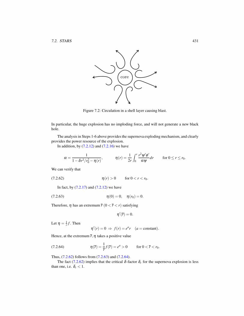
7.2. STARS 431
core
Figure 7.2: Circulation in a shell layer causing blast.
In particular, the huge explosion has no imploding force, and will not generate a new black
hole.
The analysis in Steps 1-6 above provides the supernova exploding mechanism, and clearly
provides the power resource of the explosion.
In addition, by (7.2.12) and (7.2.16) we have
α =1
1− δ r2/r20 −η(r)
, η(r) =1
2r
∫ r
0
r2ψ ′φ ′
αψdr for 0 ≤ r ≤ r0.
We can verify that
(7.2.62) η(r)> 0 for 0 < r < r0.
In fact, by (7.2.17) and (7.2.12) we have
(7.2.63) η(0) = 0, η(r0) = 0.
Therefore, η has an extremum r (0 < r < r) satisfying
η ′(r) = 0.
Let η = 1r
f . Then
η ′(r) = 0 ⇒ f (r) = ear (a = constant).
Hence, at the extremum r,η takes a positive value
(7.2.64) η(r) =1
rf (r) = ea > 0 for 0 < r < r0.
Thus, (7.2.62) follows from (7.2.63) and (7.2.64).
The fact (7.2.62) implies that the critical δ -factor δc for the supernova explosion is less
than one, i.e. δc < 1.
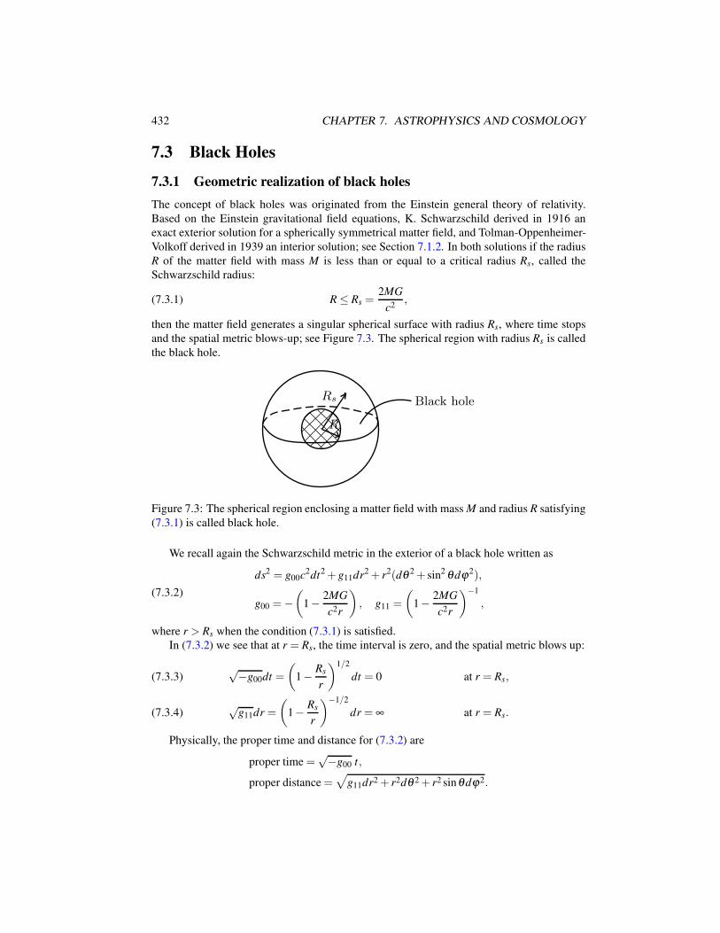
432 CHAPTER 7. ASTROPHYSICS AND COSMOLOGY
7.3 Black Holes
7.3.1 Geometric realization of black holes
The concept of black holes was originated from the Einstein general theory of relativity.
Based on the Einstein gravitational field equations, K. Schwarzschild derived in 1916 an
exact exterior solution for a spherically symmetrical matter field, and Tolman-Oppenheimer-
Volkoff derived in 1939 an interior solution; see Section 7.1.2. In both solutions if the radius
R of the matter field with mass M is less than or equal to a critical radius Rs, called the
Schwarzschild radius:
(7.3.1) R ≤ Rs =2MG
c2,
then the matter field generates a singular spherical surface with radius Rs, where time stops
and the spatial metric blows-up; see Figure 7.3. The spherical region with radius Rs is called
the black hole.
R
Rs Black hole
Figure 7.3: The spherical region enclosing a matter field with mass M and radius R satisfying
(7.3.1) is called black hole.
We recall again the Schwarzschild metric in the exterior of a black hole written as
(7.3.2)
ds2 = g00c2dt2 + g11dr2 + r2(dθ 2 + sin2 θdϕ2),
g00 =−(
1− 2MG
c2r
), g11 =
(1− 2MG
c2r
)−1
,
where r > Rs when the condition (7.3.1) is satisfied.
In (7.3.2) we see that at r = Rs, the time interval is zero, and the spatial metric blows up:
√−g00dt =
(1− Rs
r
)1/2
dt = 0 at r = Rs,(7.3.3)
√g11dr =
(1− Rs
r
)−1/2
dr = ∞ at r = Rs.(7.3.4)
Physically, the proper time and distance for (7.3.2) are
proper time =√−g00 t,
proper distance =√
g11dr2 + r2dθ 2 + r2 sinθdϕ2.
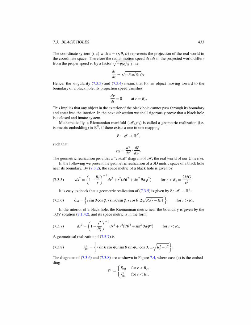
7.3. BLACK HOLES 433
The coordinate system (t,x) with x = (r,θ ,ϕ) represents the projection of the real world to
the coordinate space. Therefore the radial motion speed dr/dt in the projected world differs
from the proper speed vr by a factor√−g00/g11, i.e.
dr
dt=√−g00/g11vr.
Hence, the singularity (7.3.3) and (7.3.4) means that for an object moving toward to the
boundary of a black hole, its projection speed vanishes:
dr
dt= 0 at r = Rs.
This implies that any object in the exterior of the black hole cannot pass through its boundary
and enter into the interior. In the next subsection we shall rigorously prove that a black hole
is a closed and innate system.
Mathematically, a Riemannian manifold (M ,gi j) is called a geometric realization (i.e.
isometric embedding) in RN , if there exists a one to one mapping
~r : M → RN ,
such that
gi j =d~r
dxi· d~r
dx j.
The geometric realization provides a “visual” diagram of M , the real world of our Universe.
In the following we present the geometric realization of a 3D metric space of a black hole
near its boundary. By (7.3.2), the space metric of a black hole is given by
(7.3.5) ds2 =
(1− Rs
r
)−1
dr2 + r2(dθ 2 + sin2 θdϕ2) for r > Rs =2MG
c2.
It is easy to check that a geometric realization of (7.3.5) is given by~r : M →R4:
(7.3.6) ~rext =
r sinθ cosϕ ,r sin θ sinϕ ,r cosθ ,2√
Rs(r−Rs)
for r > Rs.
In the interior of a black hole, the Riemannian metric near the boundary is given by the
TOV solution (7.1.42), and its space metric is in the form
(7.3.7) ds2 =
(1− r2
R2s
)−1
dr2 + r2(dθ 2 + sin2 θdϕ2) for r < Rs,
A geometrical realization of (7.3.7) is
(7.3.8) ~r±int =
r sin θ cosϕ ,r sin θ sinϕ ,r cosθ ,±
√R2
s − r2
.
The diagrams of (7.3.6) and (7.3.8) are as shown in Figure 7.4, where case (a) is the embed-
ding
~r+ =
~rext for r > Rs,
~r+int for r < Rs,
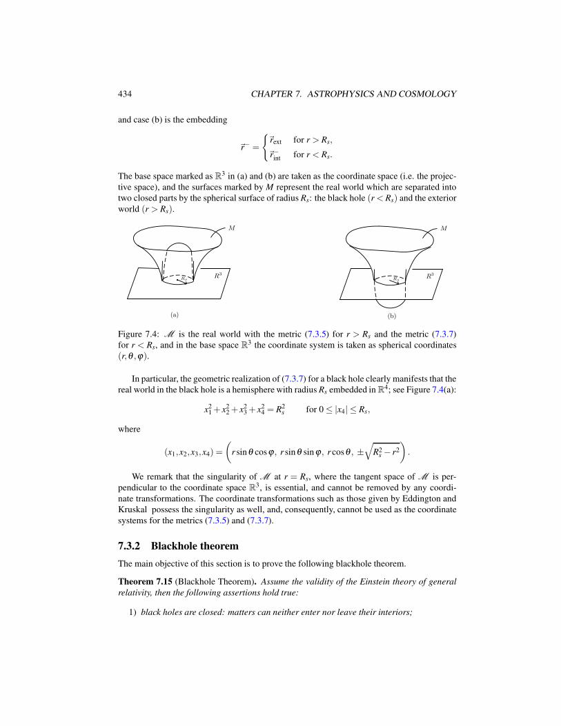
434 CHAPTER 7. ASTROPHYSICS AND COSMOLOGY
and case (b) is the embedding
~r− =
~rext for r > Rs,
~r−int for r < Rs.
The base space marked as R3 in (a) and (b) are taken as the coordinate space (i.e. the projec-
tive space), and the surfaces marked by M represent the real world which are separated into
two closed parts by the spherical surface of radius Rs: the black hole (r < Rs) and the exterior
world (r > Rs).
Rs
R3
M
Rs
R3
M
(a) (b)
Figure 7.4: M is the real world with the metric (7.3.5) for r > Rs and the metric (7.3.7)
for r < Rs, and in the base space R3 the coordinate system is taken as spherical coordinates
(r,θ ,ϕ).
In particular, the geometric realization of (7.3.7) for a black hole clearly manifests that the
real world in the black hole is a hemisphere with radius Rs embedded in R4; see Figure 7.4(a):
x21 + x2
2 + x23 + x2
4 = R2s for 0 ≤ |x4| ≤ Rs,
where
(x1,x2,x3,x4) =
(r sinθ cosϕ , r sinθ sin ϕ , r cosθ , ±
√R2
s − r2
).
We remark that the singularity of M at r = Rs, where the tangent space of M is per-
pendicular to the coordinate space R3, is essential, and cannot be removed by any coordi-
nate transformations. The coordinate transformations such as those given by Eddington and
Kruskal possess the singularity as well, and, consequently, cannot be used as the coordinate
systems for the metrics (7.3.5) and (7.3.7).
7.3.2 Blackhole theorem
The main objective of this section is to prove the following blackhole theorem.
Theorem 7.15 (Blackhole Theorem). Assume the validity of the Einstein theory of general
relativity, then the following assertions hold true:
1) black holes are closed: matters can neither enter nor leave their interiors;
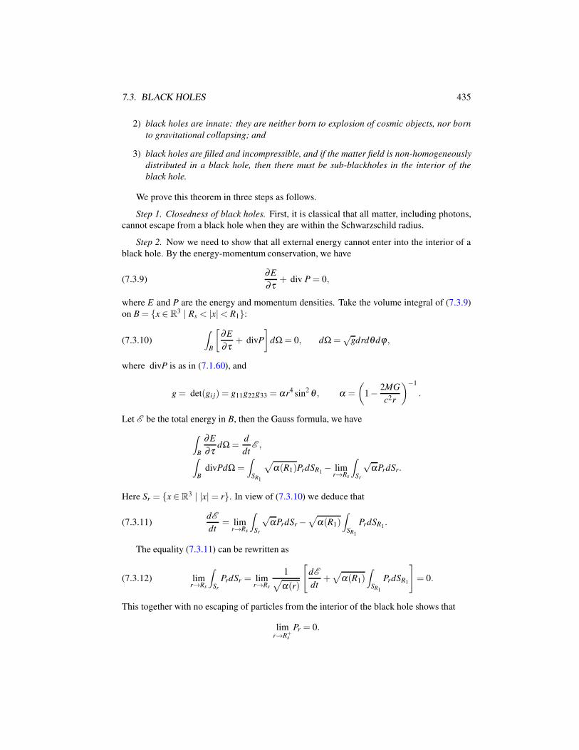
7.3. BLACK HOLES 435
2) black holes are innate: they are neither born to explosion of cosmic objects, nor born
to gravitational collapsing; and
3) black holes are filled and incompressible, and if the matter field is non-homogeneously
distributed in a black hole, then there must be sub-blackholes in the interior of the
black hole.
We prove this theorem in three steps as follows.
Step 1. Closedness of black holes. First, it is classical that all matter, including photons,
cannot escape from a black hole when they are within the Schwarzschild radius.
Step 2. Now we need to show that all external energy cannot enter into the interior of a
black hole. By the energy-momentum conservation, we have
(7.3.9)∂E
∂τ+ div P = 0,
where E and P are the energy and momentum densities. Take the volume integral of (7.3.9)
on B = x ∈ R3 | Rs < |x|< R1:
(7.3.10)
∫
B
[∂E
∂τ+ divP
]dΩ = 0, dΩ =
√gdrdθdϕ ,
where divP is as in (7.1.60), and
g = det(gi j) = g11g22g33 = αr4 sin2 θ , α =
(1− 2MG
c2r
)−1
.
Let E be the total energy in B, then the Gauss formula, we have
∫
B
∂E
∂τdΩ =
d
dtE ,
∫
BdivPdΩ =
∫
SR1
√α(R1)PrdSR1
− limr→Rs
∫
Sr
√αPrdSr.
Here Sr = x ∈ R3 | |x|= r. In view of (7.3.10) we deduce that
(7.3.11)dE
dt= lim
r→Rs
∫
Sr
√αPrdSr −
√α(R1)
∫
SR1
PrdSR1.
The equality (7.3.11) can be rewritten as
(7.3.12) limr→Rs
∫
Sr
PrdSr = limr→Rs
1√α(r)
[dE
dt+√
α(R1)
∫
SR1
PrdSR1
]= 0.
This together with no escaping of particles from the interior of the black hole shows that
limr→R+
s
Pr = 0.
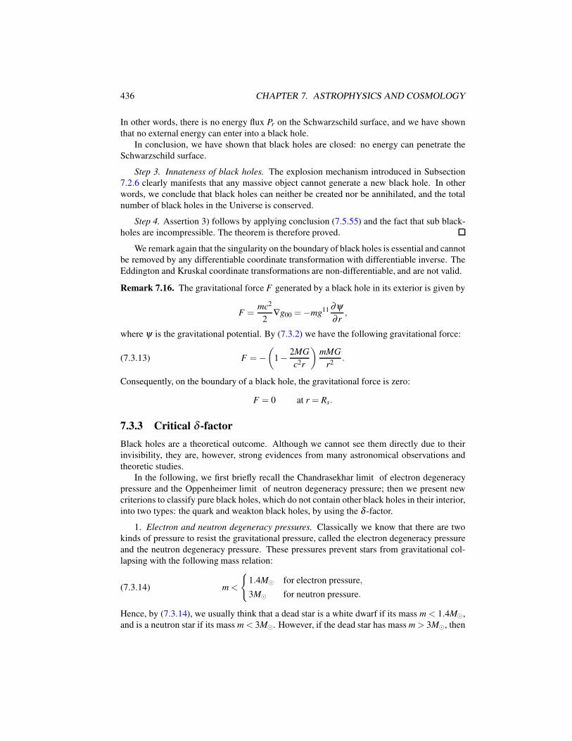
436 CHAPTER 7. ASTROPHYSICS AND COSMOLOGY
In other words, there is no energy flux Pr on the Schwarzschild surface, and we have shown
that no external energy can enter into a black hole.
In conclusion, we have shown that black holes are closed: no energy can penetrate the
Schwarzschild surface.
Step 3. Innateness of black holes. The explosion mechanism introduced in Subsection
7.2.6 clearly manifests that any massive object cannot generate a new black hole. In other
words, we conclude that black holes can neither be created nor be annihilated, and the total
number of black holes in the Universe is conserved.
Step 4. Assertion 3) follows by applying conclusion (7.5.55) and the fact that sub black-
holes are incompressible. The theorem is therefore proved.
We remark again that the singularity on the boundary of black holes is essential and cannot
be removed by any differentiable coordinate transformation with differentiable inverse. The
Eddington and Kruskal coordinate transformations are non-differentiable, and are not valid.
Remark 7.16. The gravitational force F generated by a black hole in its exterior is given by
F =mc2
2∇g00 =−mg11 ∂ψ
∂ r,
where ψ is the gravitational potential. By (7.3.2) we have the following gravitational force:
(7.3.13) F =−(
1− 2MG
c2r
)mMG
r2.
Consequently, on the boundary of a black hole, the gravitational force is zero:
F = 0 at r = Rs.
7.3.3 Critical δ -factor
Black holes are a theoretical outcome. Although we cannot see them directly due to their
invisibility, they are, however, strong evidences from many astronomical observations and
theoretic studies.
In the following, we first briefly recall the Chandrasekhar limit of electron degeneracy
pressure and the Oppenheimer limit of neutron degeneracy pressure; then we present new
criterions to classify pure black holes, which do not contain other black holes in their interior,
into two types: the quark and weakton black holes, by using the δ -factor.
1. Electron and neutron degeneracy pressures. Classically we know that there are two
kinds of pressure to resist the gravitational pressure, called the electron degeneracy pressure
and the neutron degeneracy pressure. These pressures prevent stars from gravitational col-
lapsing with the following mass relation:
(7.3.14) m <
1.4M⊙ for electron pressure,
3M⊙ for neutron pressure.
Hence, by (7.3.14), we usually think that a dead star is a white dwarf if its mass m < 1.4M⊙,
and is a neutron star if its mass m < 3M⊙. However, if the dead star has mass m > 3M⊙, then
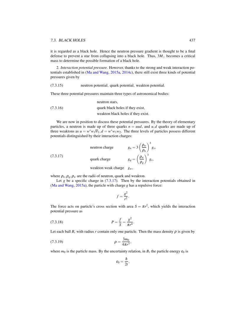
7.3. BLACK HOLES 437
it is regarded as a black hole. Hence the neutron pressure gradient is thought to be a final
defense to prevent a star from collapsing into a black hole. Thus, 3M⊙ becomes a critical
mass to determine the possible formation of a black hole.
2. Interaction potential pressure. However, thanks to the strong and weak interaction po-
tentials established in (Ma and Wang, 2015a, 2014c), there still exist three kinds of potential
pressures given by
(7.3.15) neutron potential, quark potential, weakton potential.
These three potential pressures maintain three types of astronomical bodies:
(7.3.16)
neutron stars,
quark black holes if they exist,
weakton black holes if they exist.
We are now in position to discuss these potential pressures. By the theory of elementary
particles, a neutron is made up of three quarks n = uud, and u,d quarks are made up of
three weaktons as u = w∗w1w1,d = w∗w1w2. The three levels of particles possess different
potentials distinguished by their interaction charges:
(7.3.17)
neutron charge gn = 3
(ρw
ρn
)3
gs,
quark charge gq =
(ρw
ρq
)3
gs,
weakton weak charge gw,
where ρn,ρq,ρw are the radii of neutron, quark and weakton.
Let g be a specific charge in (7.3.17). Then by the interaction potentials obtained in
(Ma and Wang, 2015a), the particle with charge g has a repulsive force:
f =g2
r2.
The force acts on particle’s cross section with area S = πr2, which yields the interaction
potential pressure as
(7.3.18) P =f
S=
g2
πr4.
Let each ball Br with radius r contain only one particle. Then the mass density ρ is given by
(7.3.19) ρ =3m0
4πr3,
where m0 is the particle mass. By the uncertainty relation, in Br the particle energy ε0 is
ε0 =h
2t,
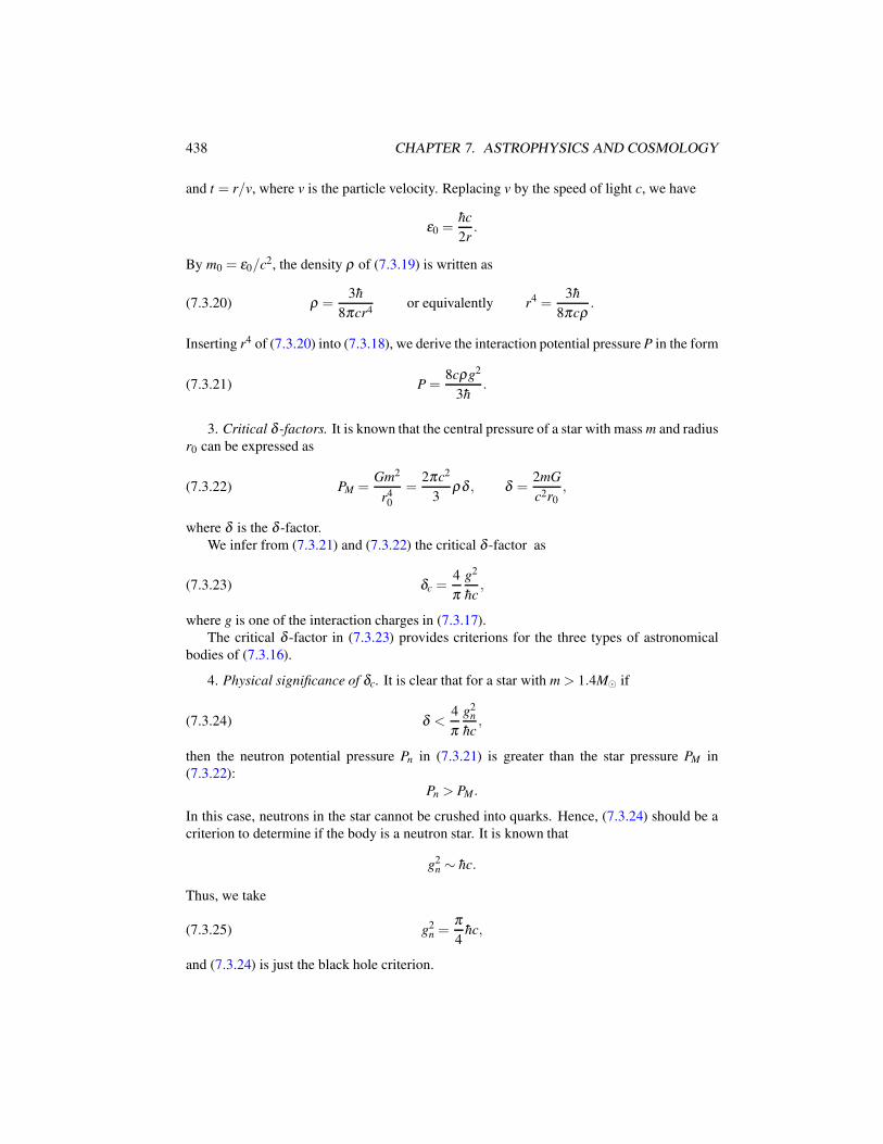
438 CHAPTER 7. ASTROPHYSICS AND COSMOLOGY
and t = r/v, where v is the particle velocity. Replacing v by the speed of light c, we have
ε0 =hc
2r.
By m0 = ε0/c2, the density ρ of (7.3.19) is written as
(7.3.20) ρ =3h
8πcr4or equivalently r4 =
3h
8πcρ.
Inserting r4 of (7.3.20) into (7.3.18), we derive the interaction potential pressure P in the form
(7.3.21) P =8cρg2
3h.
3. Critical δ -factors. It is known that the central pressure of a star with mass m and radius
r0 can be expressed as
(7.3.22) PM =Gm2
r40
=2πc2
3ρδ , δ =
2mG
c2r0
,
where δ is the δ -factor.
We infer from (7.3.21) and (7.3.22) the critical δ -factor as
(7.3.23) δc =4
π
g2
hc,
where g is one of the interaction charges in (7.3.17).
The critical δ -factor in (7.3.23) provides criterions for the three types of astronomical
bodies of (7.3.16).
4. Physical significance of δc. It is clear that for a star with m > 1.4M⊙ if
(7.3.24) δ <4
π
g2n
hc,
then the neutron potential pressure Pn in (7.3.21) is greater than the star pressure PM in
(7.3.22):
Pn > PM.
In this case, neutrons in the star cannot be crushed into quarks. Hence, (7.3.24) should be a
criterion to determine if the body is a neutron star. It is known that
g2n ∼ hc.
Thus, we take
(7.3.25) g2n =
π
4hc,
and (7.3.24) is just the black hole criterion.
7.3. BLACK HOLES 439
If the δ -factor satisfies that
(7.3.26)4
π
g2n
hc≤ δ <
4
π
g2q
hc,
then the neutrons will be crushed to become quarks and gluons. The equality (7.3.25) shows
that the star satisfying (7.3.26) must be a black hole which is composed of quarks and gluons,
and is called quark black hole.
If δ satisfies
(7.3.27)4
π
g2q
hc≤ δ <
4
π
g2w
hc,
then the quarks are crushed into weaktons, and the body is called weakton black hole.
In summary, we infer from (7.3.24), (7.3.26) and (7.3.27) the following conclusions:
(7.3.28) a body =
a neutron star if δ < δ cn and m > 1.4M⊙,
a quark black hole if δ cn < δ < δ c
q ,
a weakton black hole if δ cq < δ < δ c
w,
where
δ cj =
4
π
g2j
hcfor j = n,q,w.
5. Upper limit of the radius. Weaktons are elementary particles, which cannot be crushed.
Therefore, there is no star with δ -factor greater than δ cw. Thus there exists an upper limit for
the radius rc for astronomical bodies with mass m, determined by
2MG
c2rc
= δ cw.
Namely, the upper limit of the radius rc reads
(7.3.29) rc =πmG
2c2
hc
g2w
.
Finally we remark that since black holes cannot be compressed, the δ -factor of any as-
tronomical object cannot be less than one: δ ≥ 1. Therefore, by (7.3.25) and (7.3.26), there
exist no weakton black holes.
7.3.4 Origin of stars and galaxies
The closeness and innateness of black holes provide an excellent explanation for the origin
of planets, stars and galaxies.
In fact, all black holes are inherent. Namely, black holes exist at the very beginning of
the Universe. During the evolution of the Universe, each black hole forms a core and adsorbs
a ball of gases around it. The globes of gases eventually evolve into planets, stars and galaxy
nuclei, according to the radii or masses of the inner cores of black holes. Of course, it is
possible that several black holes can bound together to form a core of a bulk of gases.
440 CHAPTER 7. ASTROPHYSICS AND COSMOLOGY
Due to the closedness of black holes, planets, stars and galaxy nuclei are stable, which
cannot be absorbed into the inner cores of black holes and vanish.
1. Jeans theory on the origin of stars and galaxies. In the beginning of the twentieth cen-
tury, J. Jeans presented a general theory for the formation of galaxies and stars. He thought
that the Universe in the beginning was filled with chaotic gas, and various astronomical ob-
jects were formed in succession by a process of gas decomposition into bulks of clouds,
consequently forming galaxies, stars, and planets.
According to the Jeans theory, a ball of clouds with homogeneous density ρ can be held
together only if
(7.3.30) V +K ≤ 0,
where V is the total gravitational potential energy, and K is the total kinetic energy of all
particles. The potential energy V is
(7.3.31) V =−∫ R
0
GMr
r× 4πr2ρdr =−3GM2
5R,
where M is the mass of the cloud, Mr = 4πr3ρ/3, and R is the radius. The kinetic energy K
is expressed as the sum of thermal kinetic energies of all particles:
K =3
2NkT,
where N is the particle number, T is the temperature, and k is the Boltzmann constant. As-
sume that all particles have the same mass m, then N = M/m, and we have
(7.3.32) K =3M
2mkT.
Thus, by (7.3.30)-(7.3.32) we obtain that
(7.3.33)GM
R≥ 5
2mkT.
The inequality (7.3.33) is called the Jeans condition.
2. Masses of astronomical objects. The Jeans condition (7.3.33) guarantees only the
gaseous clouds being held together, and does not imply that the gas clouds can contract to
form an astronomical object. However, a black hole must attract the nebulae around it to form
a compact body.
We consider the mass relation between an astronomical object and its black hole core.
The mass M of the object is
(7.3.34) M = Mb +M1,
where Mb is the mass of the black hole, and M1 is the mass of the material attracted by this
black hole. The total binding potential energy V of this object is given by
(7.3.35) V =−∫ R
Rs
GMr
r× 4πr2ρdr,
7.3. BLACK HOLES 441
where R is the object radius, Rs is the radius of the black hole, ρ is the mass density outside
the core, and
(7.3.36) Mr = Mb +
∫ r
Rs
4πr2ρdr.
Since Rs ≪ R, we take Rs = 0 in the integrals (7.3.35) and (7.3.36). We assume that the
density ρ is a constant. Then, it follows from (7.3.35) and (7.3.36) that
V =−4πGρ
∫ R
0
[Mbr+
4π
3ρr4
]dr =−4πGρ
(MbR2
2+
4π
3× 5ρR5
).
By ρ = M1/43πR3 and Mb = M−M1, we have
(7.3.37) V =−G
R
(3
2MM1 −
9
10M2
1
).
The stability of the object requires that −V takes its maximum at some M1 such that
dV/dM1 = 0. Hence we derive from (7.3.37) that
(7.3.38) M1 =5
6M, Mb =
1
6M.
The relation (7.3.38) means that a black hole with mass Mb can form an astronomical object
with mass M = 6Mb.
3. Relation between radius and temperature. A black hole with mass Mb determines the
mass M of the corresponding astronomical system: M = 6Mb. Then, by the Jeans relation
(7.3.33), the radius R and average temperature T satisfy
(7.3.39) T =2× 6GmMb
5kR
where T is expressed as
T =3
4πR3
∫
BR
τ(x)dx,
where BR is the ball of this system, and τ(x) is the temperature distribution. Let τ = τ(r)depend only on r, then we have
(7.3.40) T =3
R3
∫ R
0r2τ(r)dr.
4. Solar system. For the Sun, M = 2× 1030kg and R = 7× 10⁸m. Hence the mass of the
solar black hole core is about
M⊙b =1
3× 1030kg,
and the average temperature has an upper limit:
T =4
5× 6.7× 10−11m3/kg · s2 × 1030kg× 1.7× 10−27kg
1.4× 10⁻²⁴kg ·m2/s2 ·K× 7× 10⁸m≃ 108K.
442 CHAPTER 7. ASTROPHYSICS AND COSMOLOGY
Table 7.1: Levels of Cosmic Structure
levels Sunstar clusters
(globular)galaxies
(spiral)clusters of
galaxiesUniverse
radius(pc) 10−8 10 105 106 1010
distance(pc) 1 103 106 108
mass(M⊙) 1 106 1011 1014 1021
density
(kg/m3)103 10−18 10−20 10−23 10−27
For the earth, M = 6× 1024kg,R = 6.4× 10⁶m. Thus we have
Meb = 1024kg, T = 3.3× 10⁴.
5. The radii of the solar and earth’s black hole cores. The radius of solar black hole is
given by
R⊙s = 500 m,
and the radius of black hole of the earth is as
Res =
3
2cm.
7.4 Galaxies
7.4.1 Introduction
Galaxy is an elementary unit in the large scale structure of our Universe, which is composed
of star clusters, stars, gases and dusts. In the following we introduce this topic.
1. Levels of cosmical structure. There are mainly five levels of cosmic structure: stars,
star clusters, galaxies, clusters of galaxies, and the Universe, and their basic scales are given
inTable 7.1.
2. Galaxy types. Galaxies consist of the following three types:
Elliptical (E), Spiral (S), irregular (Irr).
The spiral galaxies are divided into two different sequences:
normal spirals, denoted by S,
barred spirals, denoted by SB.
Elliptical galaxies have an oval appearance, which are classified into eight grades, denoted
by E0,E1, · · · ,E7, according to their apparent ellipticity e = (a− b)/a, where a is the major
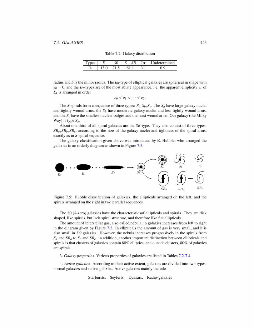
7.4. GALAXIES 443
Table 7.2: Galaxy distribution
Types E S0 S+ SB Irr Undetermined
% 13.0 21.5 61.1 3.1 0.9
radius and b is the minor radius. The E0-type of elliptical galaxies are spherical in shape with
e0 = 0, and the E7-types are of the most ablate appearance, i.e. the apparent ellipticity ek of
Ek is arranged in order
e0 < e1 < · · ·< e7.
The S-spirals form a sequence of three types: Sa,Sb,Sc. The Sa have large galaxy nuclei
and tightly wound arms, the Sb have moderate galaxy nuclei and less tightly wound arms,
and the Sc have the smallest nuclear bulges and the least wound arms. Our galaxy (the Milky
Way) is type Sb.
About one third of all spiral galaxies are the SB-type. They also consist of three types:
SBa,SBb,SBc, according to the size of the galaxy nuclei and tightness of the spiral arms,
exactly as in S-spiral sequence.
The galaxy classification given above was introduced by E. Hubble, who arranged the
galaxies in an orderly diagram as shown in Figure 7.5.
E0E4
E7 SO
Sa SbSc
SBa SBbSBc
Figure 7.5: Hubble classification of galaxies, the ellipticals arranged on the left, and the
spirals arranged on the right in two parallel sequences.
The S0 (S-zero) galaxies have the characteristicsof ellipticals and spirals. They are disk
shaped, like spirals, but lack spiral structure, and therefore like flat ellipticals.
The amount of interstellar gas, also called nebula, in galaxies increases from left to right
in the diagram given by Figure 7.2. In ellipticals the amount of gas is very small, and it is
also small in SO galaxies. However, the nebula increases progressively in the spirals from
Sa and SBa to Sc and SBc. in addition, another important distinction between ellipticals and
spirals is that clusters of galaxies contain 80% elliptics, and outside clusters, 80% of galaxies
are spirals.
3. Galaxy properties. Various properties of galaxies are listed in Tables 7.2-7.4.
4. Active galaxies. According to their active extent, galaxies are divided into two types:
normal galaxies and active galaxies. Active galaxies mainly include
Starbursts, Seyferts, Quasars, Radio-galaxies
444 CHAPTER 7. ASTROPHYSICS AND COSMOLOGY
Table 7.3: Average physical quantities
Types E Sa Sb Sc Irr
mass (M⊙) 2.0× 10¹¹ 1.6× 10¹¹ 1.3× 10¹¹ 1.6× 10¹⁰ 1× 10⁹
mass/luminosity
(m⊙/L⊙)20-70 6.6 3.6 1.4 0.9
density (M⊙/pc3) 0.16 0.08 0.025 0.013 0.003
gas mass (%) ≤ 0.2 1.3 3 20 40
Table 7.4: Properties of ellipticals and spirals
Properties ellipticals spirals
interstellarmatter non plentiful
young stars non yes
appearance elliptical shape disk shape
stellar motion random rotation
color red blue
Active galaxies are usually characterized by their extraordinary energy emision. The
starburst galaxies emit a large amount of infrared radiation, which is caused by a great number
of newly formed stars. But the three types of galaxies: Seyferts, Quasars and Radio-galaxies
are known as active galaxies because they possess a compact region at their centers that has
a much higher radiation than normal luminosity, which is called the active galactic nucleus
(AGN).
AGN generates and emits immense quantities of energy over a wide range of electromag-
netic wavelengths. Today, it is widely believed that AGN is an accretion disk generated by
a supermassive black hole. Though we have not completely confirmed evidence to show the
existence of black holes, many astronomical observations strongly suggest their existence.
The main features of active galaxies are listed in Table 7.5.
5. The Milky Way. Our own galaxy is known as the Milky Way, which is of Sb type and
has 1011 stars and an enormous quantities of clouds of gases and dusts. Its radius is about 105
ly.
The Milky Way consists of two parts: the disk and the halo. The disk has the radius of
about 5×10⁵ ly and the thick of about 5×10⁴ ly. The disk is composed of stars and nebulae,
Table 7.5: Features of active galaxies
Galaxy Type Active nuclei strong radiation Jets
Normal No no no
Starburst No yes no
Seyfert yes yes yes
Quasar yes yes yes
Radio galaxy yes yes yes
7.4. GALAXIES 445
rotating around the center of the galaxy. The Sun is 3× 10⁴ ly from the nucleus, it moves at
300km/s and has a period of 2× 10⁸ years.
The halo of the Milky Way is spherically-shaped, centered on the nucleus of the galaxy,
and has the radius of 105ly. The halo consists of less gas and roughly 120 globular clusters,
each of which has hundreds of thousands of stars and moves in an elliptical orbit around the
nucleus of the galaxy. The halo does not rotate with the disk.
6. Galaxy clusters. Galaxies are not uniformly distributed in the Universe, but aggregate
in clusters of different size. Clusters of galaxies are the largest known astronomical systems
bound by gravitational attraction. They form dense regions in the large scale structure of our
Universe. The clusters are associated with much larger, non-gravitationally bounded groups,
called superclusters.
The great regular clusters of galaxies are spherically-shaped, have roughly thousands of
galaxies, almost all of which are of E and S0 types. The regular clusters of galaxies are
typically 5× 10⁶ly in radius, and have no clear outer boundaries. Clusters are locked as
their galaxies held together by mutual gravitational attraction. However, their velocities are
too large, exceeding 103km/s, for them to remain gravitationally bound by their mutual at-
tractions. It implies the presence of either an additional invisible mass component, or an
additional attractive force besides the Newtonian gravity. This is the so called dark matter
phenomenon. Astronomical observations manifest that there are large amounts of intergalac-
tic gas which is very hot between 107 ∼ 108 K. The total mass of the gas is greater than
that of all galaxies in the cluster. The wind of intergalactic gas streaming through these fast
moving galaxies is strong enough to strip away their interstellar gas. This explains why the E
and S0 types of galaxies have less gas because their gas has been swept out by intergalactic
winds.
The other galaxy clusters are irregular. They have various sizes ranged from thousands
of members to a few tens of members. The smaller clusters are also called galaxy groups.
For example, our galaxy is a member of a galaxy group known as the local group which
possesses about 40 galaxies. The irregular clusters lack spherical symmetry in shape and
contain a mixture of all types of galaxies.
7.4.2 Galaxy dynamics
Galaxies are mainly either spiral or elliptical. Each galaxy possesses a compact core, known
as galactic nucleus, which is supermassive and spherical-shaped. Thus, the galactic dynamic
model is defined in an annular domain:
r0 < r < r1,
where r0 is the radius of galaxy nucleus and r1 the galaxy radius. In the following we develop
models for spiral and elliptical galaxies, and provide their basic consequences on galactic
dynamics.
1. Spiral galaxies. Spiral galaxies are disc-shaped, as shown in Figure 7.6. We model the
galaxy in a disc domain as
(7.4.1) D = x ∈ R2 | r0 < |x|< r1,
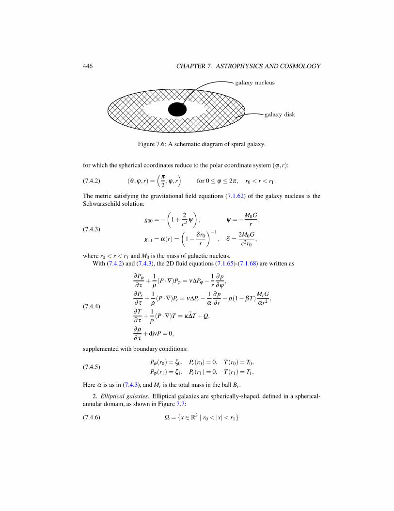
446 CHAPTER 7. ASTROPHYSICS AND COSMOLOGY
galaxy nucleus
galaxy disk
Figure 7.6: A schematic diagram of spiral galaxy.
for which the spherical coordinates reduce to the polar coordinate system (ϕ ,r):
(7.4.2) (θ ,ϕ ,r) =(π
2,ϕ ,r
)for 0 ≤ ϕ ≤ 2π , r0 < r < r1.
The metric satisfying the gravitational field equations (7.1.62) of the galaxy nucleus is the
Schwarzschild solution:
(7.4.3)
g00 =−(
1+2
c2ψ
), ψ =−M0G
r,
g11 = α(r) =
(1− δ r0
r
)−1
, δ =2M0G
c2r0
,
where r0 < r < r1 and M0 is the mass of galactic nucleus.
With (7.4.2) and (7.4.3), the 2D fluid equations (7.1.65)-(7.1.68) are written as
(7.4.4)
∂Pϕ
∂τ+
1
ρ(P ·∇)Pϕ = ν∆Pϕ − 1
r
∂ p
∂ϕ,
∂Pr
∂τ+
1
ρ(P ·∇)Pr = ν∆Pr −
1
α
∂ p
∂ r−ρ(1−β T)
MrG
αr2,
∂T
∂τ+
1
ρ(P ·∇)T = κ∆T +Q,
∂ρ
∂τ+ divP = 0,
supplemented with boundary conditions:
(7.4.5)Pϕ(r0) = ζ0, Pr(r0) = 0, T (r0) = T0,
Pϕ(r1) = ζ1, Pr(r1) = 0, T (r1) = T1.
Here α is as in (7.4.3), and Mr is the total mass in the ball Br.
2. Elliptical galaxies. Elliptical galaxies are spherically-shaped, defined in a spherical-
annular domain, as shown in Figure 7.7:
(7.4.6) Ω = x ∈R3 | r0 < |x|< r1
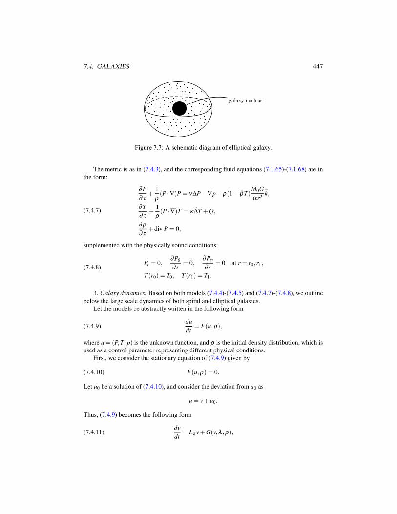
7.4. GALAXIES 447
galaxy nucleus
Figure 7.7: A schematic diagram of elliptical galaxy.
The metric is as in (7.4.3), and the corresponding fluid equations (7.1.65)-(7.1.68) are in
the form:
(7.4.7)
∂P
∂τ+
1
ρ(P ·∇)P = ν∆P−∇p−ρ(1−β T)
M0G
αr2~k,
∂T
∂τ+
1
ρ(P ·∇)T = κ∆T +Q,
∂ρ
∂τ+ div P = 0,
supplemented with the physically sound conditions:
(7.4.8)Pr = 0,
∂Pθ
∂ r= 0,
∂Pϕ
∂ r= 0 at r = r0,r1,
T (r0) = T0, T (r1) = T1.
3. Galaxy dynamics. Based on both models (7.4.4)-(7.4.5) and (7.4.7)-(7.4.8), we outline
below the large scale dynamics of both spiral and elliptical galaxies.
Let the models be abstractly written in the following form
(7.4.9)du
dt= F(u,ρ),
where u = (P,T, p) is the unknown function, and ρ is the initial density distribution, which is
used as a control parameter representing different physical conditions.
First, we consider the stationary equation of (7.4.9) given by
(7.4.10) F(u,ρ) = 0.
Let u0 be a solution of (7.4.10), and consider the deviation from u0 as
u = v+ u0.
Thus, (7.4.9) becomes the following form
(7.4.11)dv
dt= Lλ v+G(v,λ ,ρ),
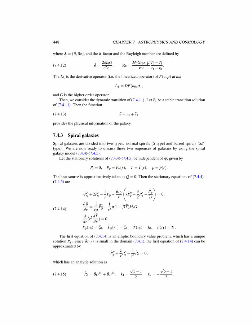
448 CHAPTER 7. ASTROPHYSICS AND COSMOLOGY
where λ = (δ ,Re), and the δ -factor and the Rayleigh number are defined by
(7.4.12) δ =2M0G
c2r0
, Re =M0Gr0r1β
κν
T0 −T1
r1 − r0
.
The Lλ is the derivative operator (i.e. the linearized operator) of F(u, p) at u0:
Lλ = DF(u0,ρ),
and G is the higher order operator.
Then, we consider the dynamic transition of (7.4.11). Let vλ be a stable transition solution
of (7.4.11). Then the function
(7.4.13) u = u0 + vλ
provides the physical information of the galaxy.
7.4.3 Spiral galaxies
Spiral galaxies are divided into two types: normal spirals (S-type) and barred spirals (SB-
type). We are now ready to discuss these two sequences of galaxies by using the spiral
galaxy model (7.4.4)-(7.4.5).
Let the stationary solutions of (7.4.4)-(7.4.5) be independent of ϕ , given by
Pr = 0, Pϕ = Pϕ(r), T = T (r), p = p(r).
The heat source is approximatively taken as Q = 0. Then the stationary equations of (7.4.4)-
(7.4.5) are
(7.4.14)
rP′′ϕ + 2P′
ϕ −1
rPϕ − δ r0
r
(rP′′
ϕ +3
2P′
ϕ − Pϕ
2r
)= 0,
∂ p
∂ r=
1
rρP2
ϕ − 1
r2ρ(1−β T)MrG,
d
dr(r2 dT
dr) = 0,
Pϕ(r0) = ζ0, Pϕ(r1) = ζ1, T (r0) = T0, T (r1) = T1.
The first equation of (7.4.14) is an elliptic boundary value problem, which has a unique
solution Pϕ . Since δ r0/r is small in the domain (7.4.1), the first equation of (7.4.14) can be
approximated by
P′′ϕ +
2
rP′
ϕ − 1
r2Pϕ = 0,
which has an analytic solution as
(7.4.15) Pϕ = β1rk1 +β2rk2 , k1 =
√5− 1
2, k2 =−
√5+ 1
2.
7.4. GALAXIES 449
By the boundary conditions in (7.4.14), we obtain that
(7.4.16) β1 =r
k20 ζ1 − r
k21 ζ0
rk11 r
k20 − r
k10 r
k21
, β2 =r
k11 ζ0 − r
k10 ζ1
rk11 r
k20 − r
k10 r
k21
.
Thus we derive the solution of (7.4.14) as
Pϕ , T = T0 +T0 −T1
r1 − r0
r1(r0
r− 1), p =
∫ [ P2ϕ
rρ− ρG
r2(1−β T)Mr
]dr.
Make the translation
Pr → Pr, Pϕ → Pϕ + Pϕ , T → T + T , p → p+ p;
then the equations (7.4.4) and boundary conditions (7.4.5) become
(7.4.17)
∂Pϕ
∂τ+
1
ρ(P ·∇)Pϕ = ν∆Pϕ − (
Pϕ
r+
dPϕ
dr)Pr −
1
r
∂ p
∂ϕ,
∂Pr
∂τ+
1
ρ(P ·∇)Pr = ν∆Pr +
2Pϕ
αrPϕ +
ρβ MrG
αr2T − 1
α
∂ p
∂ r,
∂T
∂τ+
1
ρ(P ·∇)T = κ∆T +
r0r1
ρr2γPr −
1
ρrPϕ
∂T
∂ϕ,
div P = 0,
P = 0, T = 0 at r = r0,r1,
where r = (T0 −T1)/(r1 − r0).The eigenvalue equations of (7.4.17) are given by
(7.4.18)
−∆Pϕ +1
ν(
Pϕ
r+
dPϕ
dr)Pr +
1
rν
∂ p
∂ϕ= λ Pϕ ,
−∆Pr −2Pϕ
ανrPϕ − ρβ MrG
ανr2T +
1
αν
∂ p
∂ r= λ Pr,
−∆T +1
ρrPϕ
∂T
∂ϕ− r0r1γ
κρr2Pr = λ T,
div P = 0,
P = 0, T = 0 at r = r0,r1.
The eigenvalues λ of (7.4.18) are discrete (not counting multiplicity):
λ1 > λ2 > · · ·> λk > · · · , λk →−∞ as k → ∞.
The first eigenvalue λ1 and first eigenfunctions
(7.4.19) Φ = (P0ϕ ,P
0r ,T
0)
450 CHAPTER 7. ASTROPHYSICS AND COSMOLOGY
dictate the dynamic behaviors of spiral galaxies, which are determined by the physical pa-
rameters:
(7.4.20) ζ0,ζ1,r0,r1,κ ,ν,β ,γ =T0 −T1
r1 − r0
, δ =2M0G
c2r0
, Mr = M0 + 4π
∫ r1
r0
r2ρdr.
Based on the dynamic transition theory in (Ma and Wang, 2013b), we have the following
physical conclusions:
• If the parameters in (7.4.20) make the first eigenvalue λ1 < 0, then the spiral galaxy is
of S0-type.
• If λ1 > 0, then the galaxy is one of the types Sa,Sb,Sc,SBa,SBb,SBc, depending on the
structure of (P0ϕ ,P
0r ) in (7.4.19).
• Let λ1 > 0 and the first eigenvector (P0ϕ ,P
0r ) of (7.4.19) have the vortex structure as
shown in Figure 7.8. Then the number of spiral arms of the galaxy is k/2, where k is
the vortex number of (P0ϕ ,P
0r ). Hence, if k = 2, the galaxy is of the SBc-type.
Figure 7.8: The vortex structure of the first eigenvector (P0ϕ ,P
0r ).
The reason behind the number of spiral arms being k/2 is as follows. First the number of
vortices in Figure 7.8 is even, and each pair of vortices have reversed orientations. Second, if
the orientation of a vortex matches that of the stationary solution Pϕ(r) of (7.4.14), then the
superposition of Pϕ(r) and P0ϕ of (7.4.19) gives rise to an arm; otherwise, the counteraction
of Pϕ(r) and P0ϕ with reversed orientations reduces the energy momentum density, and the
region becomes nearly void.
Remark 7.17. There are three terms in (7.4.18), which may generate the transition of (7.4.17):
F1 =
(0,−k1T
r2,−k2Pr
r2
), k2 =
ρβ MrG
αν, k2 =
r0r1γ
κρ,
F2 =
(1
ν
(Pϕ
r+
dPϕ
dr
)Pr,−
2Pϕ
ανrPϕ ,0
),
F3 =
(− 1
2α2r
dα
dr
∂
∂ r(rPϕ),
1
2α
∂
∂ r(
1
α
dα
drPr),0
).
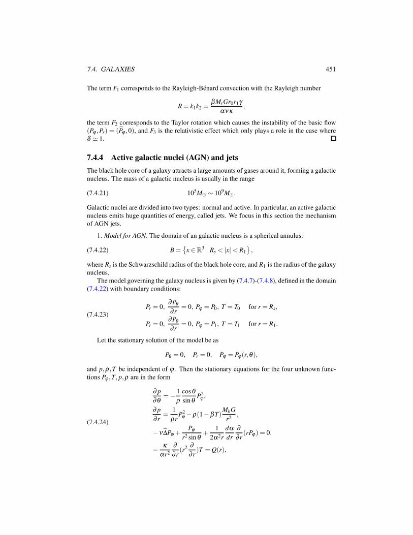
7.4. GALAXIES 451
The term F1 corresponds to the Rayleigh-Benard convection with the Rayleigh number
R = k1k2 =β MrGr0r1γ
ανκ,
the term F2 corresponds to the Taylor rotation which causes the instability of the basic flow
(Pϕ ,Pr) = (Pϕ ,0), and F3 is the relativistic effect which only plays a role in the case where
δ ≃ 1.
7.4.4 Active galactic nuclei (AGN) and jets
The black hole core of a galaxy attracts a large amounts of gases around it, forming a galactic
nucleus. The mass of a galactic nucleus is usually in the range
(7.4.21) 105M⊙ ∼ 109M⊙.
Galactic nuclei are divided into two types: normal and active. In particular, an active galactic
nucleus emits huge quantities of energy, called jets. We focus in this section the mechanism
of AGN jets.
1. Model for AGN. The domain of an galactic nucleus is a spherical annulus:
(7.4.22) B =
x ∈ R3 | Rs < |x|< R1
,
where Rs is the Schwarzschild radius of the black hole core, and R1 is the radius of the galaxy
nucleus.
The model governing the galaxy nucleus is given by (7.4.7)-(7.4.8), defined in the domain
(7.4.22) with boundary conditions:
(7.4.23)
Pr = 0,∂Pθ
∂ r= 0, Pϕ = P0, T = T0 for r = Rs,
Pr = 0,∂Pθ
∂ r= 0, Pϕ = P1, T = T1 for r = R1.
Let the stationary solution of the model be as
Pθ = 0, Pr = 0, Pϕ = Pϕ(r,θ ),
and p,ρ ,T be independent of ϕ . Then the stationary equations for the four unknown func-
tions Pϕ ,T, p,ρ are in the form
(7.4.24)
∂ p
∂θ=− 1
ρ
cosθ
sinθP2
ϕ ,
∂ p
∂ r=
1
ρrP2
ϕ −ρ(1−β T)MbG
r2,
−ν∆Pϕ +Pϕ
r2 sinθ+
1
2α2r
dα
dr
∂
∂ r(rPϕ) = 0,
− κ
αr2
∂
∂ r(r2 ∂
∂ r)T = Q(r),
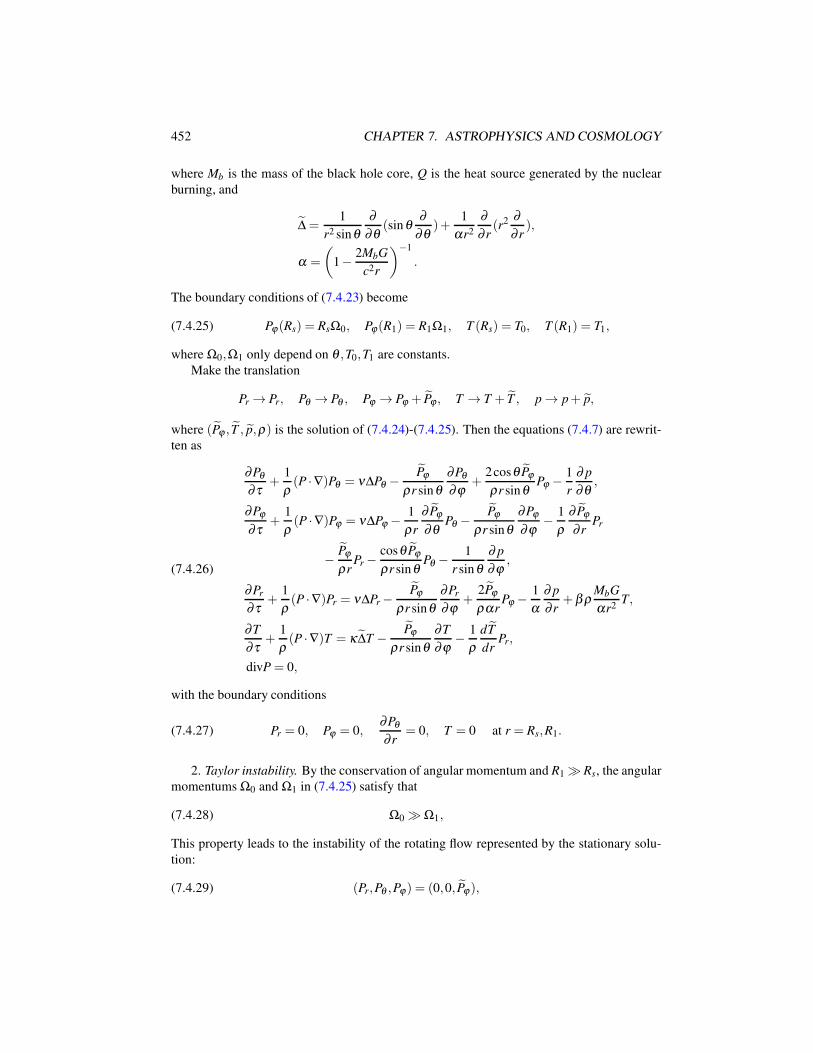
452 CHAPTER 7. ASTROPHYSICS AND COSMOLOGY
where Mb is the mass of the black hole core, Q is the heat source generated by the nuclear
burning, and
∆ =1
r2 sinθ
∂
∂θ(sin θ
∂
∂θ)+
1
αr2
∂
∂ r(r2 ∂
∂ r),
α =
(1− 2MbG
c2r
)−1
.
The boundary conditions of (7.4.23) become
(7.4.25) Pϕ(Rs) = RsΩ0, Pϕ(R1) = R1Ω1, T (Rs) = T0, T (R1) = T1,
where Ω0,Ω1 only depend on θ ,T0,T1 are constants.
Make the translation
Pr → Pr, Pθ → Pθ , Pϕ → Pϕ + Pϕ , T → T + T , p → p+ p,
where (Pϕ , T , p,ρ) is the solution of (7.4.24)-(7.4.25). Then the equations (7.4.7) are rewrit-
ten as
(7.4.26)
∂Pθ
∂τ+
1
ρ(P ·∇)Pθ = ν∆Pθ −
Pϕ
ρr sinθ
∂Pθ
∂ϕ+
2cosθ Pϕ
ρr sinθPϕ − 1
r
∂ p
∂θ,
∂Pϕ
∂τ+
1
ρ(P ·∇)Pϕ = ν∆Pϕ − 1
ρr
∂ Pϕ
∂θPθ −
Pϕ
ρr sinθ
∂Pϕ
∂ϕ− 1
ρ
∂ Pϕ
∂ rPr
− Pϕ
ρrPr −
cosθ Pϕ
ρr sinθPθ −
1
r sin θ
∂ p
∂ϕ,
∂Pr
∂τ+
1
ρ(P ·∇)Pr = ν∆Pr −
Pϕ
ρr sinθ
∂Pr
∂ϕ+
2Pϕ
ραrPϕ − 1
α
∂ p
∂ r+β ρ
MbG
αr2T,
∂T
∂τ+
1
ρ(P ·∇)T = κ∆T − Pϕ
ρr sinθ
∂T
∂ϕ− 1
ρ
dT
drPr,
divP = 0,
with the boundary conditions
(7.4.27) Pr = 0, Pϕ = 0,∂Pθ
∂ r= 0, T = 0 at r = Rs,R1.
2. Taylor instability. By the conservation of angular momentum and R1 ≫ Rs, the angular
momentums Ω0 and Ω1 in (7.4.25) satisfy that
(7.4.28) Ω0 ≫ Ω1,
This property leads to the instability of the rotating flow represented by the stationary solu-
tion:
(7.4.29) (Pr,Pθ ,Pϕ) = (0,0, Pϕ),
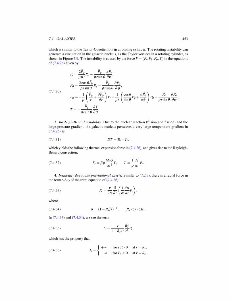
7.4. GALAXIES 453
which is similar to the Taylor-Couette flow in a rotating cylinder. The rotating instability can
generate a circulation in the galactic nucleus, as the Taylor vortices in a rotating cylinder, as
shown in Figure 7.9. The instability is caused by the force F = (Fr,Fθ ,Fϕ ,T ) in the equations
of (7.4.26) given by
(7.4.30)
Fr =2Pϕ
ραrPϕ − Pϕ
ρr sinθ
∂Pr
∂ϕ,
Fθ =2cosθ Pϕ
ρr sinθPϕ − Pϕ
ρr sinθ
∂Pθ
∂ϕ,
Fϕ =− 1
ρ
(Pϕ
r+
∂ Pϕ
∂ r
)Pr −
1
ρr
(cosθ
sinθPϕ +
∂ Pϕ
∂θ
)Pθ −
Pϕ
ρr sinθ
∂Pϕ
∂ϕ,
T =− Pϕ
ρr sinθ
∂T
∂θ.
3. Rayleigh-Benard instability. Due to the nuclear reaction (fusion and fission) and the
large pressure gradient, the galactic nucleus possesses a very large temperature gradient in
(7.4.25) as
(7.4.31) DT = T0 −T1,
which yields the following thermal expansion force in (7.4.26), and gives rise to the Rayleigh-
Benard convection:
(7.4.32) Fr = β ρMbG
αr2T, T =
1
ρ
dT
drPr.
4. Instability due to the gravitational effects. Similar to (7.2.7), there is a radial force in
the term ν∆ur of the third equation of (7.4.26):
(7.4.33) Fr =ν
2α
∂
∂ r
(1
α
dα
drPr
),
where
(7.4.34) α = (1−Rs/r)−1, Rs < r < R1.
In (7.4.33) and (7.4.34), we see the term
(7.4.35) fr =ν
1−Rs/r
R2s
r4Pr,
which has the property that
(7.4.36) fr =
+∞ for Pr > 0 at r = Rs,
−∞ for Pr < 0 at r = Rs.
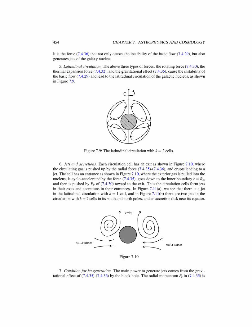
454 CHAPTER 7. ASTROPHYSICS AND COSMOLOGY
It is the force (7.4.36) that not only causes the instability of the basic flow (7.4.29), but also
generates jets of the galaxy nucleus.
5. Latitudinal circulation. The above three types of forces: the rotating force (7.4.30), the
thermal expansion force (7.4.32), and the gravitational effect (7.4.35), cause the instability of
the basic flow (7.4.29) and lead to the latitudinal circulation of the galactic nucleus, as shown
in Figure 7.9.
Figure 7.9: The latitudinal circulation with k = 2 cells.
6. Jets and accretions. Each circulation cell has an exit as shown in Figure 7.10, where
the circulating gas is pushed up by the radial force (7.4.35)-(7.4.36), and erupts leading to a
jet. The cell has an entrance as shown in Figure 7.10, where the exterior gas is pulled into the
nucleus, is cyclo-accelerated by the force (7.4.35), goes down to the inner boundary r = Rs,
and then is pushed by Fθ of (7.4.30) toward to the exit. Thus the circulation cells form jets
in their exits and accretions in their entrances. In Figure 7.11(a), we see that there is a jet
in the latitudinal circulation with k = 1 cell, and in Figure 7.11(b) there are two jets in the
circulation with k = 2 cells in its south and north poles, and an accretion disk near its equator.
exit
entranceentrance
Figure 7.10
7. Condition for jet generation. The main power to generate jets comes from the gravi-
tational effect of (7.4.35)-(7.4.36) by the black hole. The radial momentum Pr in (7.4.35) is
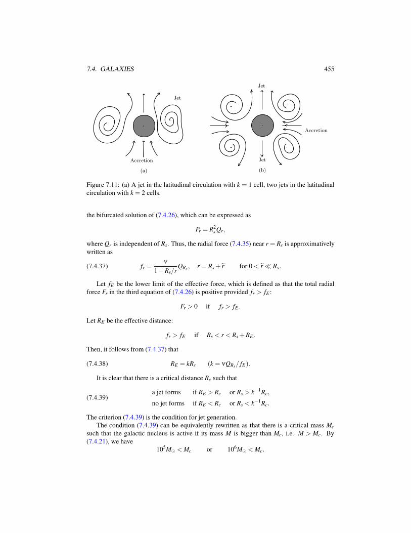
7.4. GALAXIES 455
Jet
Accretion
(a) (b)
Accretion
Jet
Jet
Figure 7.11: (a) A jet in the latitudinal circulation with k = 1 cell, two jets in the latitudinal
circulation with k = 2 cells.
the bifurcated solution of (7.4.26), which can be expressed as
Pr = R2s Qr,
where Qr is independent of Rs. Thus, the radial force (7.4.35) near r = Rs is approximatively
written as
(7.4.37) fr =ν
1−Rs/rQRs , r = Rs + r for 0 < r ≪ Rs.
Let fE be the lower limit of the effective force, which is defined as that the total radial
force Fr in the third equation of (7.4.26) is positive provided fr > fE :
Fr > 0 if fr > fE .
Let RE be the effective distance:
fr > fE if Rs < r < Rs +RE .
Then, it follows from (7.4.37) that
(7.4.38) RE = kRs (k = νQRs/ fE).
It is clear that there is a critical distance Rc such that
(7.4.39)a jet forms if RE > Rc or Rs > k−1Rc,
no jet forms if RE < Rc or Rs < k−1Rc.
The criterion (7.4.39) is the condition for jet generation.
The condition (7.4.39) can be equivalently rewritten as that there is a critical mass Mc
such that the galactic nucleus is active if its mass M is bigger than Mc, i.e. M > Mc. By
(7.4.21), we have
105M⊙ < Mc or 106M⊙ < Mc.
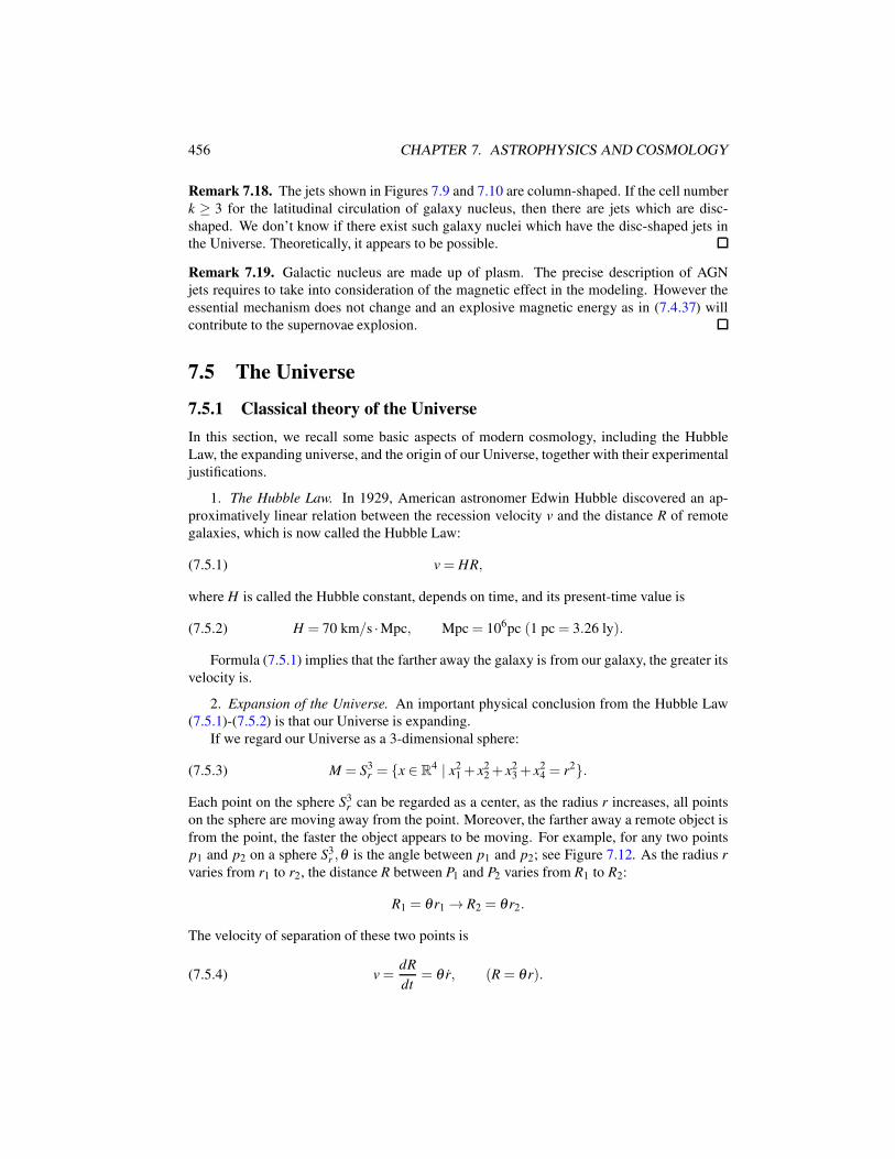
456 CHAPTER 7. ASTROPHYSICS AND COSMOLOGY
Remark 7.18. The jets shown in Figures 7.9 and 7.10 are column-shaped. If the cell number
k ≥ 3 for the latitudinal circulation of galaxy nucleus, then there are jets which are disc-
shaped. We don’t know if there exist such galaxy nuclei which have the disc-shaped jets in
the Universe. Theoretically, it appears to be possible.
Remark 7.19. Galactic nucleus are made up of plasm. The precise description of AGN
jets requires to take into consideration of the magnetic effect in the modeling. However the
essential mechanism does not change and an explosive magnetic energy as in (7.4.37) will
contribute to the supernovae explosion.
7.5 The Universe
7.5.1 Classical theory of the Universe
In this section, we recall some basic aspects of modern cosmology, including the Hubble
Law, the expanding universe, and the origin of our Universe, together with their experimental
justifications.
1. The Hubble Law. In 1929, American astronomer Edwin Hubble discovered an ap-
proximatively linear relation between the recession velocity v and the distance R of remote
galaxies, which is now called the Hubble Law:
(7.5.1) v = HR,
where H is called the Hubble constant, depends on time, and its present-time value is
(7.5.2) H = 70 km/s ·Mpc, Mpc = 106pc (1 pc = 3.26 ly).
Formula (7.5.1) implies that the farther away the galaxy is from our galaxy, the greater its
velocity is.
2. Expansion of the Universe. An important physical conclusion from the Hubble Law
(7.5.1)-(7.5.2) is that our Universe is expanding.
If we regard our Universe as a 3-dimensional sphere:
(7.5.3) M = S3r = x ∈ R
4 | x21 + x2
2 + x23 + x2
4 = r2.
Each point on the sphere S3r can be regarded as a center, as the radius r increases, all points
on the sphere are moving away from the point. Moreover, the farther away a remote object is
from the point, the faster the object appears to be moving. For example, for any two points
p1 and p2 on a sphere S3r ,θ is the angle between p1 and p2; see Figure 7.12. As the radius r
varies from r1 to r2, the distance R between P1 and P2 varies from R1 to R2:
R1 = θ r1 → R2 = θ r2.
The velocity of separation of these two points is
(7.5.4) v =dR
dt= θ r, (R = θ r).
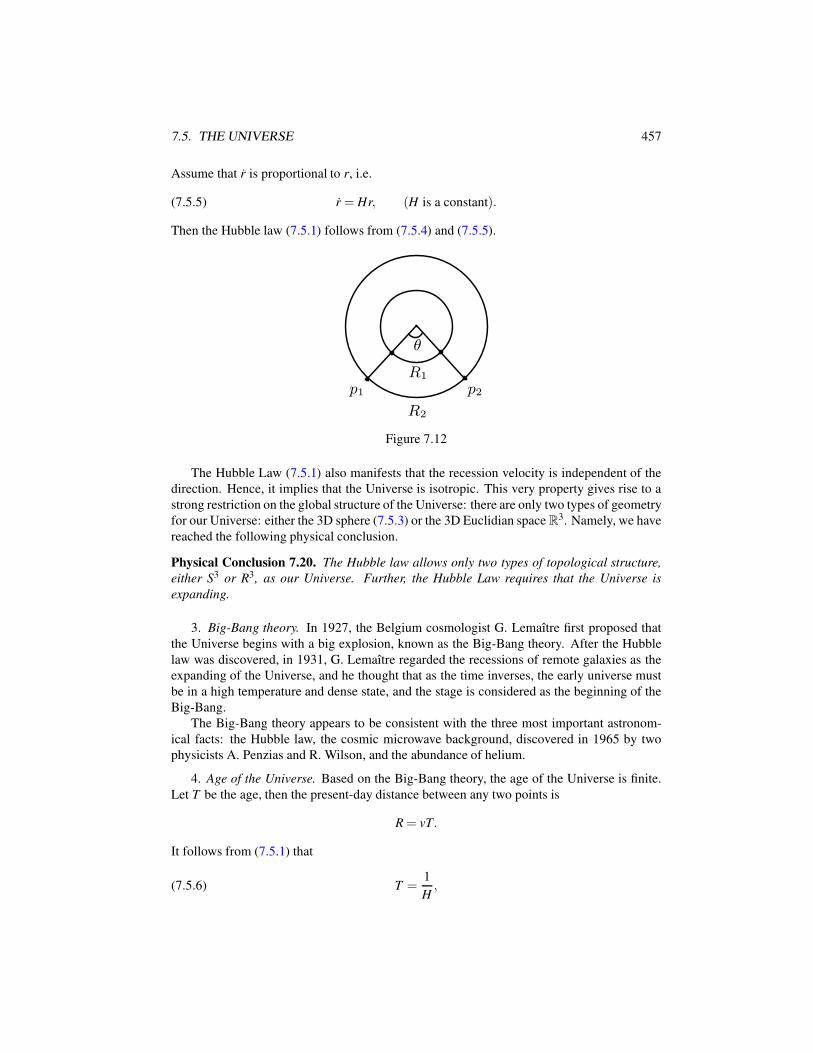
7.5. THE UNIVERSE 457
Assume that r is proportional to r, i.e.
(7.5.5) r = Hr, (H is a constant).
Then the Hubble law (7.5.1) follows from (7.5.4) and (7.5.5).
θ
p1
R1
p2
R2
Figure 7.12
The Hubble Law (7.5.1) also manifests that the recession velocity is independent of the
direction. Hence, it implies that the Universe is isotropic. This very property gives rise to a
strong restriction on the global structure of the Universe: there are only two types of geometry
for our Universe: either the 3D sphere (7.5.3) or the 3D Euclidian space R3. Namely, we have
reached the following physical conclusion.
Physical Conclusion 7.20. The Hubble law allows only two types of topological structure,
either S3 or R3, as our Universe. Further, the Hubble Law requires that the Universe is
expanding.
3. Big-Bang theory. In 1927, the Belgium cosmologist G. Lemaıtre first proposed that
the Universe begins with a big explosion, known as the Big-Bang theory. After the Hubble
law was discovered, in 1931, G. Lemaıtre regarded the recessions of remote galaxies as the
expanding of the Universe, and he thought that as the time inverses, the early universe must
be in a high temperature and dense state, and the stage is considered as the beginning of the
Big-Bang.
The Big-Bang theory appears to be consistent with the three most important astronom-
ical facts: the Hubble law, the cosmic microwave background, discovered in 1965 by two
physicists A. Penzias and R. Wilson, and the abundance of helium.
4. Age of the Universe. Based on the Big-Bang theory, the age of the Universe is finite.
Let T be the age, then the present-day distance between any two points is
R = vT.
It follows from (7.5.1) that
(7.5.6) T =1
H,
458 CHAPTER 7. ASTROPHYSICS AND COSMOLOGY
where H is the Hubble constant. We infer then from (7.5.2) and (7.5.6) the age T of the
Universe as
(7.5.7) T = 1.4× 10¹⁰ year.
As we approximatively regard the recession velocity v of remote galaxies as the speed of
light, i.e. v ≃ c, the age (7.5.7) is also considered as the radius of the Universe.
5. Structure of universes. A central topic in modern cosmology is to investigate both the
global topological and geometrical structure of the Universe. A fundamental principle of cos-
mology, called cosmological principle, states that ignoring local irregularities, the Universe
is homogeneous and isotropic.
The cosmological principle is compatible with the Hubble law: Physical Conclusion 7.20,
and can be equivalently stated in the following form.
Theorem 7.21 (Topological Structure of the Universe). The global topological structure of
the Universe is either S3 or R3.
6. Global geometrical structure. Based on the Cosmological Principle 7.21, three physi-
cists A. Friedmann (1922), G. Lemaıtre (1927), H. P. Robertson (1935), and a mathematician
A. G. Walker (1936), independently derived the globally geometrical structure of the Uni-
verse.
Theorem 7.22 (Geometrical Structure of the Universe). The Riemannian metric of 4D space-
time manifold satisfying the Cosmological Principle 7.21 takes the following form
(7.5.8) ds2 =−c2dt2 +R(t)
[dr2
1− kr2+ r2(dθ 2 + sin2 θdϕ2)
],
where R(t) is the scalar factor representing the radius of the Universe, which depends only
on time t, and k = 1,0,−1 stand for the sign of space scalar curvature in the following sense:
(7.5.9)
k = 1 : M = S3 the 3D sphere with scalar curvature =1
R2,
k = 0 : M = R3 the 3D flat Euclidean space,
k =−1 : M = L3 the Lobachevsky space with scalar curvature =− 1
R2,
where the Lobachevsky space L3 has the same topological structure as R3.
Historically, Theorem 7.22 was rigorously proved by Robertson and Walker, and was
assumed by Friedmann and Lemaıtre to derive the field equations satisfied by R(t).
7. The Newton cosmology. The Newton cosmology is based on the Newton Gravitational
Law. By Cosmological Principle (Roos, 2003), the universe is spherically symmetric. For
any reference point p ∈ M , the motion equation of an object with distance r from p is
(7.5.10)d2r
dt2=−GM(r)
r2,
7.5. THE UNIVERSE 459
where M(r) = 4πr3ρ/3, and ρ is the mass density. Thus, (7.5.10) can be rewritten as follows
(7.5.11) r′′ =−4
3πGrρ .
Make the nondimensional
r = R(t)r0,
where R(t) is the scalar factor, which is the same as in the FLRW metric (Ma and Wang,
2014e). Let ρ0 be the density at R = 1. Then we have
(7.5.12) ρ = ρ0/R3.
Thus, equation (7.5.11) is expressed as
(7.5.13) R′′ =−4πG
3
ρ0
R2,
which is the dynamic equation of Newtonian cosmology.
Multiplying both sides of (7.5.13) by R′ we have
d
dt(R2 − 8πG
3
ρ0
r) = 0.
Hence, (7.5.13) is equivalent to the equation
(7.5.14) R2 =8πG
3
ρ0
R−κ ,
where κ is a constant, and we shall see that κ = kc2, and k =−1,0, or 1.
8. The Friedmann cosmology. The nonzero components of the Friedmann metric are
g00 =−1, g11 =R2
1− kr2, g22 = R2r2, g33 = R2r2 sin2 θ .
Again by the Cosmological Principle (Roos, 2003), the energy-momentum tensor of the Uni-
verse is in the form
Tµν =
pc2 0 0 0
0 g11 p 0 0
0 0 g22 p 0
0 0 0 g33 p
.
By the Einstein gravitational field equations
Rµν =−8πG
c4(Tµν −
1
2gµνT ),
Dµ Tµν = 0,
we derive three independent equations
R =−4πG
3
(ρ +
3p
c2
)R,(7.5.15)
RR+ 2R2+ 2kc2 = 4πG(
ρ − p
c2
)R2,(7.5.16)
ρ =−3
(R
R
)(ρ +
p
c2
),(7.5.17)
460 CHAPTER 7. ASTROPHYSICS AND COSMOLOGY
where R,ρ , p are the unknown functions.
Equations (7.5.15)-(7.5.17) are called the Friedmann cosmological model, from which we
can derive the Newtonian cosmology equations (7.5.14). To see this, by (7.5.15) and (7.5.16),
we have
(7.5.18)
(R
R
)2
=−kc2
R2+
8πG
3ρ .
By the approximate p/c2 ≃ 0, (7.5.12) follows from (7.5.17). Then we deduce (7.5.14) from
(7.5.18) and (7.5.12).
From the equation (7.5.18), the density ρc corresponding to the case k = 0 is
(7.5.19) ρc =3
8πG
(R
R
)2
=3
8πGH2,
where H = R/R is the Hubble constant, and by (7.5.2) we have
(7.5.20) ρc = 10−26kg/m3.
Thus, by the Friedmann model we can deduce the following conclusions.
Conclusions of Friedmann Cosmology 7.23. 1) By (7.5.18) we can see that
(7.5.21)
ρ > ρc ⇔ k = 1 the Universe is closed : M = S3,
ρ = ρc ⇔ k = 0 the Universe is open : M = R3,
ρ < ρc ⇔ k =−1 the Universe is open : M = L3.
2) Let E0 be the total kinetic energy of the Universe, M is the mass, then we have
(7.5.22) E0 =
3
5
GM2
Rfor k = 0,
2
3π
GM2
R− 1
2Mc2 for k = 1,
where the first term represents the total gravitational bound potential energy, and the second
term is the energy resisting curvature tensor.
3) By (7.5.18), R 6≡ 0, and consequently the universe is dynamic.
4) By (7.5.15), R < 0, the dynamic universe is decelerating.
9. The Lemaıtre cosmology. Consider the Einstein gravitational field equations with the
cosmological constant Λ term:
(7.5.23) Rµν =−8πG
c4(Tµν −
1
2gµνT )+Λgµν , Λ > 0,
7.5. THE UNIVERSE 461
then the metric (7.5.8) satisfies the following equations
R =−4πG
3
(ρ +
3p
c2
)R+
Λc2
3R,(7.5.24)
(R
R
)2
=8πG
3ρ +
Λc2
3− kc2
R2,(7.5.25)
ρ + 3
(R
R
)(ρ +
p
c2
)= 0.(7.5.26)
The equations (7.5.24)-(7.5.26) are known as the Lemaıtre cosmological model, or the Λ-
cosmological model, which leads to the following conclusions of Λ-cosmology:
Conclusions of Λ-Cosmology 7.24.
1) The Universe is temporally open: R → ∞ as t → ∞;
2) There is a critical radius Rc, such that
the universe is decelerating for R < Rc,
the universe is accelerating for R > Rc,
where Rc ≃(
4πGρ0
Λc2
)1/3
;
3) As t → ∞ and ρ → 0, then we deduce from (7.5.25) that the cosmological radius R has
the asymptotic relation
(7.5.27) R ∼ e
√Λc2/3t as t → ∞.
Namely
R(t)/e
√Λc2/3t = const. as t → ∞;
4) The total kinetic energy E is given by
(7.5.28) E =
3
5
GM2
R+
Λ
10Mc2R2 for k = 0,
2
3π
GM2
R+
Λ
6Mc2R2 − 1
2Mc2 for k = 1.
Remark 7.25. The field equations (7.5.23) with a cosmological constant Λ lead to a special
conclusion that in the expansion process, there are a large quantities of energy to be created,
and the added energy in (7.5.28) is generated by Λ is as
1
6Mc2ΛR2(k = 1) and
Λ
10Mc2R2(k = 0).
It implies that the total energy is not conserved in the Λ-model.
462 CHAPTER 7. ASTROPHYSICS AND COSMOLOGY
7.5.2 Globular universe with boundary
If the spatial geometry of a universe is open, then by our theory of black holes developed in
Section 7.3, we have shown that the universe must be in a ball of a black hole with a fixed ra-
dius. In fact, according to the basic cosmological principle that the universe is homogeneous
and isotropic (Roos, 2003), given the energy density ρ0 > 0 of the universe, by Theorem 7.3,
the universe will always be bounded in a black hole of open ball with the Schwarzschild
radius:
Rs =
√3c2
8πGρ0
,
as the mass in the ball BRs is given by MRs = 4πR3s ρ0/3. This argument also clearly shows
that
there is no unbounded universe.
In addition, since a black hole is unable to expand and shrink, by property (7.5.55) of
black holes, all globular universes must be static.
Globular universe
We have shown that the universe is bounded, and suppose that the universe is open, i.e.
its topological structure is homeomorphic to R3, and it begins with a ball. Let E be its total
energy:
(7.5.29) E = mass+ kinetic+ thermal+Ψ,
where Ψ is the energy of all interaction fields. Let
(7.5.30) M = E/c2.
At the initial stage, all energy is concentrated in a ball with radius R0. By the theory of
black holes, the energy contained in the ball generates a black hole in R3 with radius
(7.5.31) Rs =2MG
c2,
provided Rs ≥ R0; see (7.3.1) and Figure 7.3.
Thus, if the universe is born to a ball, then it is immediately trapped in its own black hole
with the Schwarzschild radius Rs of (7.5.31). The 4D metric inside the black hole of the static
universe is given by
(7.5.32) ds2 =−ψ(r)c2dt2 +α(r)dr2 + r2(dθ 2 + sin2 θdϕ2),
where ψ and α satisfy the equations (7.1.79) and (7.1.80) with boundary conditions:
ψ → ψ , α → α as r → Rs,
where Rs is given by (7.5.31). Also, ψ , α are given via the TOV metric (7.1.40)-(7.1.41):
(7.5.33) ψ =1
4
(1− r2
R2s
), α =
(1− r2
R2s
)−1
for 0 ≤ r < Rs.
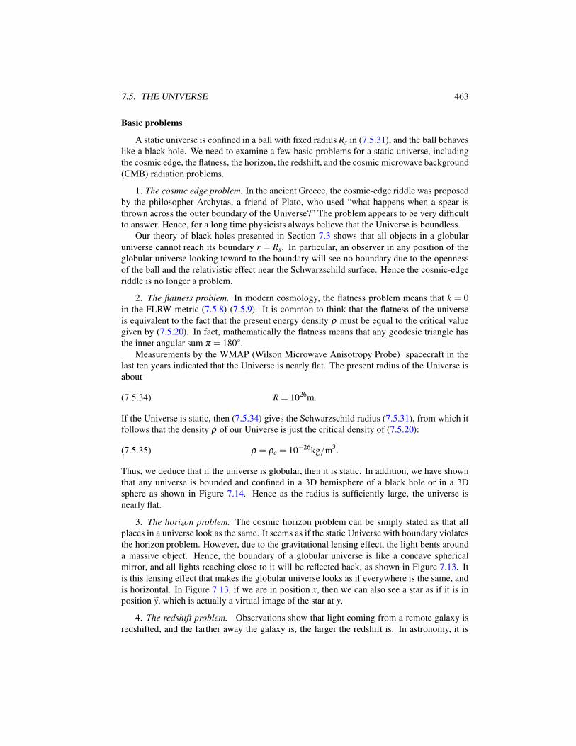
7.5. THE UNIVERSE 463
Basic problems
A static universe is confined in a ball with fixed radius Rs in (7.5.31), and the ball behaves
like a black hole. We need to examine a few basic problems for a static universe, including
the cosmic edge, the flatness, the horizon, the redshift, and the cosmic microwave background
(CMB) radiation problems.
1. The cosmic edge problem. In the ancient Greece, the cosmic-edge riddle was proposed
by the philosopher Archytas, a friend of Plato, who used “what happens when a spear is
thrown across the outer boundary of the Universe?” The problem appears to be very difficult
to answer. Hence, for a long time physicists always believe that the Universe is boundless.
Our theory of black holes presented in Section 7.3 shows that all objects in a globular
universe cannot reach its boundary r = Rs. In particular, an observer in any position of the
globular universe looking toward to the boundary will see no boundary due to the openness
of the ball and the relativistic effect near the Schwarzschild surface. Hence the cosmic-edge
riddle is no longer a problem.
2. The flatness problem. In modern cosmology, the flatness problem means that k = 0
in the FLRW metric (7.5.8)-(7.5.9). It is common to think that the flatness of the universe
is equivalent to the fact that the present energy density ρ must be equal to the critical value
given by (7.5.20). In fact, mathematically the flatness means that any geodesic triangle has
the inner angular sum π = 180.Measurements by the WMAP (Wilson Microwave Anisotropy Probe) spacecraft in the
last ten years indicated that the Universe is nearly flat. The present radius of the Universe is
about
(7.5.34) R = 1026m.
If the Universe is static, then (7.5.34) gives the Schwarzschild radius (7.5.31), from which it
follows that the density ρ of our Universe is just the critical density of (7.5.20):
(7.5.35) ρ = ρc = 10−26kg/m3.
Thus, we deduce that if the universe is globular, then it is static. In addition, we have shown
that any universe is bounded and confined in a 3D hemisphere of a black hole or in a 3D
sphere as shown in Figure 7.14. Hence as the radius is sufficiently large, the universe is
nearly flat.
3. The horizon problem. The cosmic horizon problem can be simply stated as that all
places in a universe look as the same. It seems as if the static Universe with boundary violates
the horizon problem. However, due to the gravitational lensing effect, the light bents around
a massive object. Hence, the boundary of a globular universe is like a concave spherical
mirror, and all lights reaching close to it will be reflected back, as shown in Figure 7.13. It
is this lensing effect that makes the globular universe looks as if everywhere is the same, and
is horizontal. In Figure 7.13, if we are in position x, then we can also see a star as if it is in
position y, which is actually a virtual image of the star at y.
4. The redshift problem. Observations show that light coming from a remote galaxy is
redshifted, and the farther away the galaxy is, the larger the redshift is. In astronomy, it is
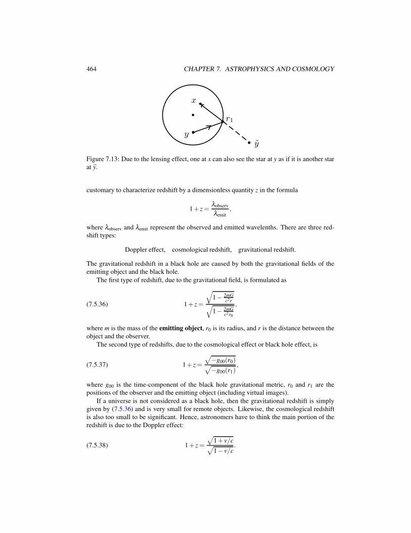
464 CHAPTER 7. ASTROPHYSICS AND COSMOLOGY
y
x
r1
y
Figure 7.13: Due to the lensing effect, one at x can also see the star at y as if it is another star
at y.
customary to characterize redshift by a dimensionless quantity z in the formula
1+ z =λobserv
λemit
,
where λobserv and λemit represent the observed and emitted wavelenths. There are three red-
shift types:
Doppler effect, cosmological redshift, gravitational redshift.
The gravitational redshift in a black hole are caused by both the gravitational fields of the
emitting object and the black hole.
The first type of redshift, due to the gravitational field, is formulated as
(7.5.36) 1+ z =
√1− 2mG
c2r√1− 2mG
c2r0
,
where m is the mass of the emitting object, r0 is its radius, and r is the distance between the
object and the observer.
The second type of redshifts, due to the cosmological effect or black hole effect, is
(7.5.37) 1+ z =
√−g00(r0)√−g00(r1)
,
where g00 is the time-component of the black hole gravitational metric, r0 and r1 are the
positions of the observer and the emitting object (including virtual images).
If a universe is not considered as a black hole, then the gravitational redshift is simply
given by (7.5.36) and is very small for remote objects. Likewise, the cosmological redshift
is also too small to be significant. Hence, astronomers have to think the main portion of the
redshift is due to the Doppler effect:
(7.5.38) 1+ z =
√1+ v/c√1− v/c
.
7.5. THE UNIVERSE 465
When v/c is small, (7.5.38) can be approximatively expressed as
(7.5.39) z ≃ v/c.
In addition, Hubble discovered that the redshift has an approximatively linear relation with
the distance:
(7.5.40) z ≃ kR, k is a constant.
Thus, the Hubble Law (7.5.1) follows from (7.5.39) and (7.5.40). It is the Hubble Law (7.5.1)
that leads to the conclusion that our Universe is expanding.
However, if we adopt the view that the globular universe is in a black hole with the
Schwarzschild radius Rs as in (7.5.31), the black hole redshift (7.5.37) cannot be ignored. By
(7.5.32) and (7.5.33), the time-component g00 for the black hole can approximatively take the
TOV solution as r near Rs:
g00 =−1
4
(1− r2
R2s
), for r near Rs.
Hence, the redshift (7.5.37) is as
(7.5.41) 1+ z =
√1− r2
0/R2s√
1− r21/R2
s
for r0,r1 < Rs.
It is known that for a remote galaxy, r1 is close to the boundary r = Rs. Therefore by (7.5.41)
we have
z →+∞ as r1 → Rs.
It reflects the redshifts observed from most remote objects. If the object is a virtual image as
shown in Figure 7.13, then its position is the reflection point r1. Thus, we see that even if the
remote object is not moving, its redshift can still be very large.
5. CMB problem. In 1965, two physicists A. Penzias and R. Wilson discovered the low-
temperature cosmic microwave background (CMB) radiation, which fills our Universe, and
it is ever regarded as the Big-Bang product. However, for a static closed Universe, it is the
most natural thing that there exists a CMB, because the Universe is a black-body and CMB
is a result of black-body radiation.
6. None expanding Universe. As the energy of the Universe is given, the maximal
radius, i.e. the Schwarzschild radius Rs, is determined, and the boundary is invariant. In fact,
a globular universe must fill the ball with the Schwarzschild radius, although the distribution
of the matter in this ball may be slightly non-homogenous. The main reason is that if the
universe has a radius R smaller than Rs, then it must contain at least a sub-black hole with
radius R0 as follows
R0 =
√R
Rs
R.
In Section 7.5.4 we shall discuss this topic.
466 CHAPTER 7. ASTROPHYSICS AND COSMOLOGY
7.5.3 Spherical Universe without boundary
Bounded universe has finite energy and space, and our Universe is bounded as we have
demonstrated in the last section. Besides the globular universe, another type of bounded
universe is the spherically-shaped corresponding to the k = 1 case in the Friedmann model
(7.5.15)-(7.5.17).
A globular universe must be static. With the same argument, a spherical closed universe
have to be static as well. In this subsection, we are devoted to investigate the spherical
cosmology.
1. Cosmic radius. For a static spherical universe, its radius Rc satisfies that
Rc = 0, Rc = 0.
By the Friedmann equation (7.5.18), it leads to that
(7.5.42) R2c =
3c2
8πGρ.
For a 3D sphere, its volume V is given by
V = 2π2R3.
Thus, ρ = M/2π2R3c , and by (7.5.43) we get the radius Rc as
(7.5.43) Rc =4MG
3πc2.
This value (7.5.43) is also the maximal radius for a (possibly) oscillatory spherical universe.
2. Negative pressure. By (7.5.15) and Rc = 0, the pressure is negative:
(7.5.44) p =−ρc2
3.
In order to resist the gravitational pulling, it is natural that there is a negative pressure in a
static universe, which originates from three sources:
thermal expanding, radiation pressure, and dark energy.
These three types of forces are repulsive, and therefore yield the negative pressure as given
by (7.5.44).
In fact, in our Universe both thermal and radiation (microwave radiation) pressures are
very small. The main negative pressure is generated by the so called “dark energy”. In
(Ma and Wang, 2014e), we have shown that the dark energy is the repulsive gravitational
effect for a remote object of great distance. From the field theoretical point view, dark energy
is an effect of the dual gravitational field Ψµ in the PID-induced gravitational field equations
(4.4.10) discovered by the authors.
3. Equivalence. It seems that both spherical and globular geometries are very different.
However, in the following we show that they are equivalent in cosmology. In fact, as the
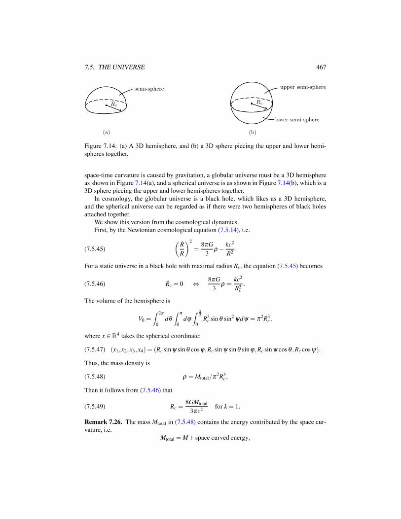
7.5. THE UNIVERSE 467
Rc
semi-sphere
(a)
Rc
upper semi-sphere
(b)
lower semi-sphere
Figure 7.14: (a) A 3D hemisphere, and (b) a 3D sphere piecing the upper and lower hemi-
spheres together.
space-time curvature is caused by gravitation, a globular universe must be a 3D hemisphere
as shown in Figure 7.14(a), and a spherical universe is as shown in Figure 7.14(b), which is a
3D sphere piecing the upper and lower hemispheres together.
In cosmology, the globular universe is a black hole, which likes as a 3D hemisphere,
and the spherical universe can be regarded as if there were two hemispheres of black holes
attached together.
We show this version from the cosmological dynamics.
First, by the Newtonian cosmological equation (7.5.14), i.e.
(7.5.45)
(R
R
)2
=8πG
3ρ − kc2
R2.
For a static universe in a black hole with maximal radius Rc, the equation (7.5.45) becomes
(7.5.46) Rc = 0 ⇔ 8πG
3ρ =
kc2
R2c
.
The volume of the hemisphere is
V0 =∫ 2π
0dθ∫ π
0dϕ∫ π
2
0R3
c sinθ sin2 ψdψ = π2R3c ,
where x ∈R4 takes the spherical coordinate:
(7.5.47) (x1,x2,x3,x4) = (Rc sinψ sinθ cosϕ ,Rc sin ψ sinθ sinϕ ,Rc sin ψ cosθ ,Rc cosψ).
Thus, the mass density is
(7.5.48) ρ = Mtotal/π2R3c ,
Then it follows from (7.5.46) that
(7.5.49) Rc =8GMtotal
3πc2for k = 1.
Remark 7.26. The mass Mtotal in (7.5.48) contains the energy contributed by the space cur-
vature, i.e.
Mtotal = M+ space curved energy,
468 CHAPTER 7. ASTROPHYSICS AND COSMOLOGY
where M is the mass of the flat space. By the invariance of density,
M/4π
3R3
c = Mtotal/π2R3c,
we get the relation
(7.5.50) Mtotal =3π
4M.
With the flat space mass (7.5.50), from (7.5.49) we get the Schwarzschild radius Rs = Rc for
the cosmic black hole as follows
Rs = 2GM/c2.
It means that the globular universe is essentially hemispherically-shaped. In particular the
relation (7.5.50) can be generated to an arbitrary region Ω ⊂ R3, i.e.
(7.5.51) MΩ;total =VΩ
|Ω|MΩ,
where MΩ is the flat space mass in Ω,MΩ;total is the curved space mass, |Ω| is the volume of
flat Ω,
VΩ =
∫
Ω
√gdx, g = det(gi j),
and gi j (1 ≤ i, j ≤ 3) is the spatial gravitational metric.
Now, we return to the Friedmann model (7.5.18) with k = 1, which has the same form as
that of the globular dynamic equation (7.5.45), and is of the same maximal radius Rc as that
in (7.5.49). Hence, it is natural that a static spherical universe is considered as if there were
two hemispherical black holes attached together. In fact, the static spherical universe forms
an entire black hole as a closed space.
4. Basic problems. Since a static spherical universe is equivalent to two globular universes
to be pieced together along with their boundary, an observer in its hemisphere is as if one is in
a globular universe. Hence, the basic problems – the cosmic edge problem, flatness problem,
horizon problem, and CMB problem– can be explained in the same fashion.
The redshift problem is slightly different, and the gravitational redshift is given by
(7.5.52) 1+ z =1√
−g00(r),
where r is the distance between the light source and the observer, and g00 is the time-
component of the gravitational metric.
Due to the horizon of sphere, for an arbitrary point on a spherical universe, its opposite
hemisphere relative to the point plays a similar role as a black hole. Hence, in the redshift
formula (7.5.52), g00 can be approximatively taken as the Schwarzschild solution for distant
objects as follows
−g00 = 1− Rs
r, Rs =
2MG
c2, r = 2Rs − r for 0 ≤ r < Rs,
7.5. THE UNIVERSE 469
where M is the cosmic mass of hemisphere, and r is the distance from the light source to the
opposite radial point, and r is from the light source to the point. Hence, formula (7.5.52) can
be approximatively written as
(7.5.53) 1+ z =1√
α(r)(1− Rsr)=
√2Rs − r√
α(r)(Rs − r)for 0 < r < Rs.
where
α(0) = 2, α(Rs) = 1, α ′(r)< 0.
We see from (7.5.53) that the redshift z → ∞ as r → Rs, and, consequently, we cannot see
objects in the opposite hemisphere. Intuitively, α(r) represents the gravitational effect of the
matter in the hemisphere of the observer.
5. Physical conclusions. In either case, globular or spherical, the universe is equivalent
to globular universe(s). It is not originated from a Big-bang, is static, and confined in a black
hole in the sense as addressed above. The observed mass M and the implicit mass Mtotal have
the relation
(7.5.54) Mtotal = 2× 3π
4M = 3πM/2,
which is derived by (7.5.50) adding the mass of another hemisphere.
The implicit mass Mtotal of (7.5.54) contains the dark matter. In (Ma and Wang, 2014e),
both the dark matter Mtotal −M and the dark energy (i.e. the negative pressure (7.5.44)) are
just a property of gravity.
7.5.4 New cosmology
We start with two difficulties encountered in modern cosmology.
First, if the Universe were born to a Big-Bang and expanded continuously, then in the
expansion process it would generate successively a large number of black holes, whose radii
vary as follows:
(7.5.55)
√R0
Rs
R0 ≤ r ≤√
R
Rs
R, R0 < R ≤ Rs =2MG
c2,
where M is the total mass in the universe, R0 is the initial radius, R is the expanding radius,
and r is the radius of sub-black holes.
To see this, we consider a homogeneous universe with radius R < Rs. Then the mass
density ρ is given by
(7.5.56) ρ =3M
4πR3.
On the other hand, by Theorem 7.3, the condition for a ball Br with radius r to form a black
hole is that the mass Mr in Br satisfies that
(7.5.57)Mr
r=
c2
2G.
470 CHAPTER 7. ASTROPHYSICS AND COSMOLOGY
By (7.5.56), we have
Mr =4π
3r3ρ =
r3
R3M.
Then it follows from (7.5.57) that
(7.5.58) r =
√R
Rs
R.
Actually, in general for a ball Br in a universe with radius R < Rs, if its mass Mr satisfies
(7.5.57) then it will form a black hole, and its radius r satisfies that
r ≤√
R
Rs
R.
In particular, there must exist a black hole whose radius r is as in (7.5.58). Thus, we derive
the conclusion (7.5.55).
Based on (7.5.55) we can deduce that if the Universe were born to a Big-Bang and contin-
uously expands, then it would contain many black holes with smaller ones being embedded
in the larger ones. In particular, the Universe would contain a huge black hole whose radius
r is almost equal to the cosmic radius Rs. This is not what we observed in our Universe.
The second difficulty of modern cosmology concerns with the Hubble Law (7.5.1), which
is restated as v = HR, where c/H = Rs. Consider a remote object with mass M0, then the
observed mass Mobser is given by Mobser =M0√1− v2
c2
. Consequently, the corresponding gravita-
tional force F to the observer with mass m is
F =−mMobserG
r2=− mM0G
r2
√1− v2
c2
=− mM0G
r2
√1− H2
c2 r2
=− mM0G
r2√
1− r2
R2s
.
It is clear then that as r → Rs, F →−∞. This is clearly not what is observed.
In conclusion, we have rigorously derived the following new theory of cosmology:
Theorem 7.27. Assume a) the Einstein theory of general relativity, and b) the principle of
cosmological principle that the universe is homogeneous and isotropic. Then the following
assertions hold true for our Universe:
1) All universes are bounded, are not originated from a Big-Bang, and are static; and
2) The topological structure of our Universe can only be the 3D sphere such that to each
observer, the corresponding equator with the observer at the center of the hemisphere
can be viewed as the black hole horizon.
Theorem 7.28. If we assume only a) the Einstein theory of general relativity, and b’) the
universe is homogeneous. Then all universes can only be either a 3D sphere as given in
Theorem 7.27, or a globular universe, which is a 3D open ball BRs of radius Rs, forming the
interior of a black hole with Rs as its Schwarzschild radius. In the later case, the Universe is
also static, is not originated from a Big-Bang, and the matter fills the entire Universe. Also,
the following assertions hold true:
7.6. THEORY OF DARK MATTER AND DARK ENERGY 471
1) The cosmic observable mass M and the total mass Mtotal, which includes both M and
the non-observable mass due to the space curvature energy, satisfy the following rela-
tion
(7.5.59) Mtotal =
3πM/2 for the spherical structure,
3πM/4 for the globular structure.
The difference Mtotal −M can be regarded as the dark matter;
2) The static Universe has to possess a negative pressure to balance the gravitational at-
tracting force. The negative pressure is actually the effect of the gravitational repelling
force, also called dark energy; and
3) Both dark matter and dark energy are a property of gravity, which is reflected in both
space-time curvature, and the attracting and repulsive gravitational forces in different
scales of the Universe. This law of gravity is precisely described by the new gravita-
tional field equations (4.4.10); see also (Ma and Wang, 2014e).
We end this section with three remarks and observations.
First, astronomical observations have shown that the measurable mass M is about one
fifth of total mass Mtotal. By (7.5.59), for the spherical universe,
Mtotal = 4.7M.
This relation also suggest that the spherical universe case fits better the current understanding
for our Universe.
Second, due to the horizon of sphere, for an arbitrary point in a spherical universe, its
opposite hemisphere relative to the point is as if it is a black hole. Hence the main contribution
to the redshifts is from the effect of the black hole, as explicitly given by (7.5.53).
Third, in modern cosmology, the view of expanding universe was based essentially on
the Friedmann model and the Hubble Law. The observations can accurately measure the
distances and redshifts for some galaxies, which allowed astronomers to get both measured
and theoretical data, and their deviation led to the conclusion that the expanding universe is
accelerating. The misunderstanding comes from the perception that the Doppler redshift is
the main source of redshifts.
7.6 Theory of Dark Matter and Dark energy
7.6.1 Dark energy and dark matter phenomena
1. Dark matter and Rubin rotational curve. In astrophysics, dark matter is an unknown form
of matter, which appears only participating in gravitational interaction, but does not emit nor
absorb electromagnetic radiations.
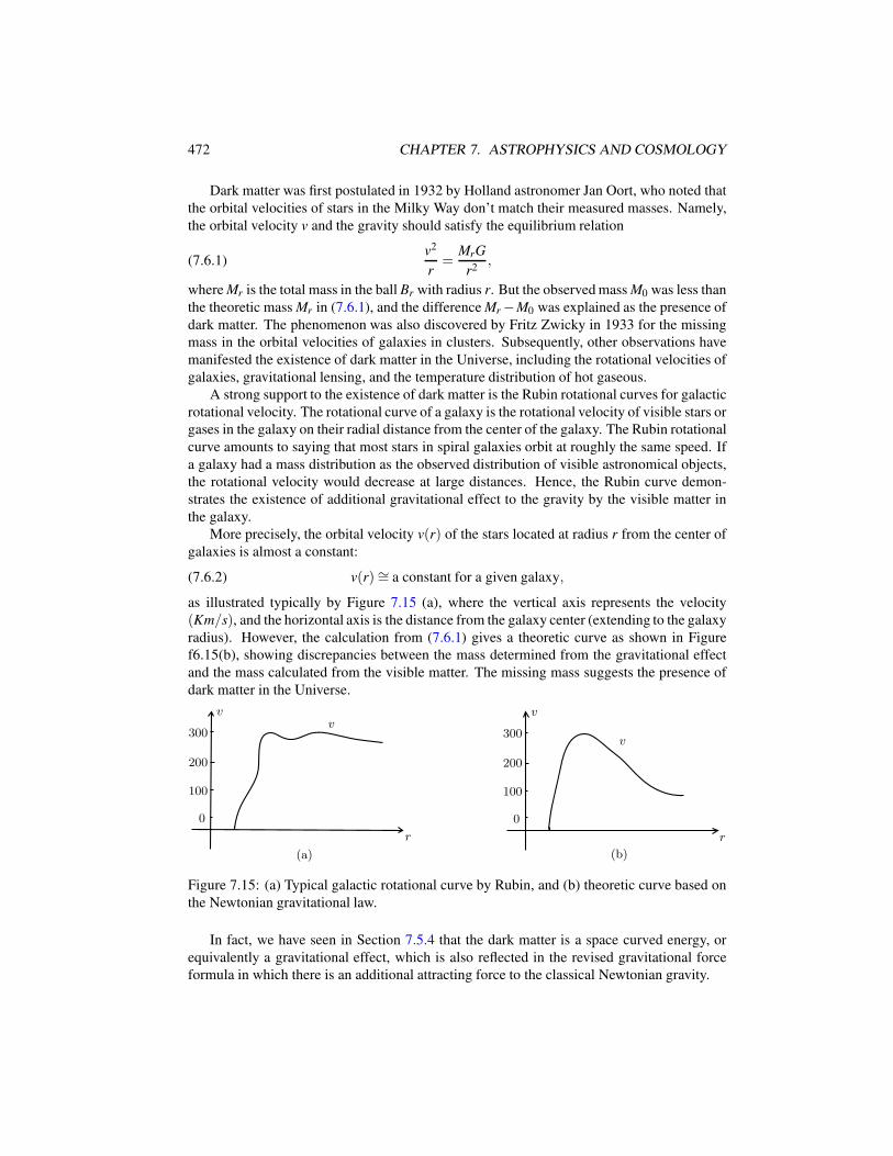
472 CHAPTER 7. ASTROPHYSICS AND COSMOLOGY
Dark matter was first postulated in 1932 by Holland astronomer Jan Oort, who noted that
the orbital velocities of stars in the Milky Way don’t match their measured masses. Namely,
the orbital velocity v and the gravity should satisfy the equilibrium relation
(7.6.1)v2
r=
MrG
r2,
where Mr is the total mass in the ball Br with radius r. But the observed mass M0 was less than
the theoretic mass Mr in (7.6.1), and the difference Mr −M0 was explained as the presence of
dark matter. The phenomenon was also discovered by Fritz Zwicky in 1933 for the missing
mass in the orbital velocities of galaxies in clusters. Subsequently, other observations have
manifested the existence of dark matter in the Universe, including the rotational velocities of
galaxies, gravitational lensing, and the temperature distribution of hot gaseous.
A strong support to the existence of dark matter is the Rubin rotational curves for galactic
rotational velocity. The rotational curve of a galaxy is the rotational velocity of visible stars or
gases in the galaxy on their radial distance from the center of the galaxy. The Rubin rotational
curve amounts to saying that most stars in spiral galaxies orbit at roughly the same speed. If
a galaxy had a mass distribution as the observed distribution of visible astronomical objects,
the rotational velocity would decrease at large distances. Hence, the Rubin curve demon-
strates the existence of additional gravitational effect to the gravity by the visible matter in
the galaxy.
More precisely, the orbital velocity v(r) of the stars located at radius r from the center of
galaxies is almost a constant:
(7.6.2) v(r)∼= a constant for a given galaxy,
as illustrated typically by Figure 7.15 (a), where the vertical axis represents the velocity
(Km/s), and the horizontal axis is the distance from the galaxy center (extending to the galaxy
radius). However, the calculation from (7.6.1) gives a theoretic curve as shown in Figure
f6.15(b), showing discrepancies between the mass determined from the gravitational effect
and the mass calculated from the visible matter. The missing mass suggests the presence of
dark matter in the Universe.
v
0
100
200
300v
r
(a)
v
0
100
200
300v
r
(b)
Figure 7.15: (a) Typical galactic rotational curve by Rubin, and (b) theoretic curve based on
the Newtonian gravitational law.
In fact, we have seen in Section 7.5.4 that the dark matter is a space curved energy, or
equivalently a gravitational effect, which is also reflected in the revised gravitational force
formula in which there is an additional attracting force to the classical Newtonian gravity.
7.6. THEORY OF DARK MATTER AND DARK ENERGY 473
2. Dark energy. Dark energy was first proposed in 1990’s, which was based on the
hypotheses that the Universe is expanding.
The High-z Supernova Search Team in 1998 and the Supernova Cosmology Project in
1999 published their precisely measured data of the distances of supernovas and the redshifts.
The observations indicated that the measured and theoretical data have a deviation, which
was explained, based on the Hubble Law and the Friedmann model, as the acceleration of
the expanding universe. The accelerating expansion is widely accepted as an evidence of the
existence of dark energy.
However, based on the new cosmology postulated in the last section, the dark energy is
a field energy form of gravitation which balances the gravitational attraction to maintain the
homogeneity and stability of the Universe.
7.6.2 PID cosmological model and dark energy
We have shown in (Ma and Wang, 2014e) that both dark matter and dark energy are a property
of gravity. Dark matter and dark energy are reflected in two aspects: a) the large scale space
curved structure of the Universe caused by gravity, and b) the gravitational attracting and
repelling aspects of gravity. In this section, we mainly explore the nature of dark energy in
aspect a) using the PID-induced cosmological model.
PID cosmological model
According to Theorem 7.22, the metric of a homogeneous spherical universe is of the
form
(7.6.3) ds2 =−c2dt2 +R2
[dr2
1− r2+ r2(dθ 2 + sin2 θdϕ2)
],
where R = R(t) is the cosmic radius. The PID induced gravitational field equations are given
by
(7.6.4) Rµν =−8πG
c4(Tµν −
1
2gµνT )− (∇µνφ − 1
2gµνΦ),
where Φ = gαβ Dαβ φ , and φ depends only on t.
The nonzero components of Rµν read as
R00 =3
c2
1
RRtt ,
Rkk =− 1
c2R2gkk(RR′′
tt + 2R2t + 2c2) for 1 ≤ k ≤ 3,
474 CHAPTER 7. ASTROPHYSICS AND COSMOLOGY
and by Tµν = diag(c2ρ ,g11 p,g22 p,g33 p), we have
T00 −1
2g00T =
c2
2
(ρ +
3p
c2
),
Tkk −1
2gkkT =
c2
2gkk
(ρ − p
c2
)for 1 ≤ k ≤ 3,
φ00 −1
2g00Φ =
1
2c2
(φtt −
3Rt
Rφt
),
φkk −1
2gkkΦ =
1
2c2gkk
(φtt +
Rt
Rφt
)for 1 ≤ k ≤ 3.
Thus, we derive from (7.6.4) two independent field equations as
R′′ =−4πG
3
(ρ +
3p
c2
)R− 1
6φ ′′R+
1
2R′φ ′,(7.6.5)
R′′
R+ 2
(R′
R
)2
+2c2
R2= 4πG
(ρ − p
c2
)+
1
2φ ′′+
1
2
R′
Rφ ′.(7.6.6)
We infer from (7.6.5) and (7.6.6) that
(7.6.7) (R′)2 =8πG
3R2ρ +
1
3R2φ ′′− c2.
By the Bianchi identity:
∇µ(∇µνφ +8πG
c4Tµν) = 0,
we deduce that
(7.6.8) φ ′′′+3R′
Rφ ′′ =−8πG
(ρ ′+
3R′
Rρ +
3R′
R
p
c2
).
It is known that the energy density ρ and the cosmic radius R (also called the scale factor)
satisfy the relation:
(7.6.9) ρ =ρ0
R3, ρ0 the density at R = 1.
Hence, it follows from (7.6.9) that
ρ ′ =−3ρR′/R.
Thus, (7.6.8) is rewritten as
(7.6.10) φ ′′′+3R′
Rφ ′′ =−24πG
c2
R′
Rp.
In addition, making the transformation
(7.6.11) φ ′′ =ψ
R3,
7.6. THEORY OF DARK MATTER AND DARK ENERGY 475
then, from (7.6.5), (7.6.7) and (7.6.9)-(7.6.11) we can deduce that
(7.6.12) (R′)2φ ′ = 0.
Denote ϕ = φ ′′, by (7.6.12), the equations (7.6.5), (7.6.7) and (7.6.10) can be rewritten in
the form
(7.6.13)
R′′ =−4πG
3
(ρ +
3p
c2+
ϕ
8πG
)R,
(R′)2 =1
3(8πGρ +ϕ)R2 − c2,
ϕ ′+3R′
Rϕ =−24πG
c2
R′
Rp.
Only two equations in (7.6.13) are independent. However, there are three unknown func-
tions R,ϕ , p in (7.6.13). Hence, we need to add an additional equation, the equation of state,
as follows:
(7.6.14) p = f (ρ ,ϕ).
Based on Theorem 7.27, the model describing the static Universe is the equation (7.6.14)
together with the stationary equations of (7.6.13), which are equivalent to the form
(7.6.15)
ϕ =−8πG
(ρ +
3p
c2
),
p =− c4
8πGR2.
The equations (7.6.14) and (7.6.15) provide a theoretic basis for the static Universe, in-
cluding the dark energy.
Now, we need to determine the explicit expression for the equation (7.6.14) of state. It is
natural to postulate that the equation of state is linear. Hence, (7.6.14) can be written as
(7.6.16) p =c2
G(α1ϕ −α2Gρ),
where α1 and α2 are nondimensional parameter, which will be determined by the observed
data.
The equations (7.6.15) and (7.6.16) are the PID cosmological model, where the cosmo-
logical significants of R, p,ϕ ,ρ are as follows:
(7.6.17)
R the cosmic radius (of the 3D spherical universe),
p the negative pressure, generated by the repulsive aspect of gravity,
ϕ represents the dual gravitational potential,
ρ the cosmic density, given by3M
4πR3=
Mtotal
π2R3,
where M and Mtotal are as in Remark 7.26.
476 CHAPTER 7. ASTROPHYSICS AND COSMOLOGY
Here, we remark that in the classical Einstein field equations where φ = 0, the relation
(7.6.9) still holds true, by which we can deduce that p = 0. It implies that the Friedmann
equations has no stationary solution for k 6= 0, and has only stationary R = 0 for k = 0.
Therefore, the PID gravitational theory is essential for establishing a static cosmological
model.
Theory of dark energy
In the static cosmology, dark energy is defined in the following manner. Let Eob be the
observed energy, and R be the cosmic radius. We define the observable mass and the total
mass as follows:
Mob =Eob
c2,(7.6.18)
MT =Rc2
2G.(7.6.19)
If MT > Mob, then the difference
(7.6.20) ∆E = ET −Eob
is called the dark energy.
The CMB measurement and the WMAP analysis indicate that the difference ∆E in (7.6.20)
is positive,
∆E > 0,
which is considered as another evidence for the presence of dark energy.
From the PID cosmological model (7.6.15)-(7.6.17), we see that the dark energy ∆E in
(7.6.20) is essentially due to the dual gravitational potential ϕ . In fact, we infer from (7.6.15)
that
(7.6.21)ϕ = 0 ⇔ R = 2MobG/c2 (i.e. ∆E = 0),
ϕ > 0 ⇔ ∆E > 0.
Hence, dark energy is generated by the dual gravitational field. This fact is reflected in the
PID gravitational force formula derived in subsections hereafter.
If we can measure precisely, with astronomical observations, the energy (7.6.18) and the
cosmic radius R (i.e. MT of (7.6.19)), then we can obtain a relation between the parameters
α1 and α2 in (7.6.16). In fact, we deduce from (7.6.15) and (7.6.16) that
(7.6.22) ρ +β p
c2= 0, β =
1+ 24πα1
α2 + 8πα1
.
As we get
(7.6.23)∆M
Mob
=MT −Mob
Mob
= k (k > 0).
Then by (7.6.22) and
ρ =3Mob
4πR3, p =− c4
8πGR2,
7.6. THEORY OF DARK MATTER AND DARK ENERGY 477
we obtain from (7.6.22) that
(7.6.24) 3α2 = 24kπα1 + k+ 1.
By the relation (7.6.24) from (7.6.22), we can also derive, in the same fashion as above,
the dark energy formula (7.6.23).
7.6.3 PID gravitational interaction formula
Consider a central gravitational field generated by a ball Br0with radius r0 and mass M. It is
known that the metric of the central field at r > r0 can be written in the form
(7.6.25) ds2 =−euc2dt2 + evdr2 + r2(dθ 2 + sin2 θdϕ2),
and u = u(r),v = v(r).In the exterior of Br0
, the energy-momentum is zero, i.e.
Tµν = 0, for r > r0.
Hence, the PID gravitational field equation for the metric (7.6.25) is given by
(7.6.26) Rµν −1
2gµνR =−∇µνφ , r > r0.
where φ = φ(r) is a scalar function of r.
By (7.1.25) and (7.1.26), we have
R00 −1
2g00R =−1
reu−v
[v′+
1
r(ev − 1)
],
R11 −1
2g11R =−1
r
[u′− 1
r(ev − 1)
],
R22 −1
2g22R =− r2
2e−v
[u′′+
(1
2u′+
1
r
)(u′− v′)
],
∇00φ =−1
2eu−vu′φ ′,
∇11φ = φ ′′− 1
2v′φ ′,
∇22φ =−re−vφ ′.
Thus, the fields equations (7.6.26) are as follows
(7.6.27)
v′+1
r(ev − 1) =− r
2u′φ ′,
u′− 1
r(ev − 1) = r(φ ′′− 1
2v′φ ′),
u′′+
(1
2u′+
1
r
)(u′− v′) =−2
rφ ′.
478 CHAPTER 7. ASTROPHYSICS AND COSMOLOGY
Now we are ready to deduce from (7.6.27) the PID gravitational interaction formula as
follows.
First, we infer from (7.6.27) that
u′+ v′ =rφ ′′
1+ r2φ ′ ,
u′− v′ =1
1− r2φ ′
[2
r(ev − 1)+ rφ ′′
].
Consequently,
(7.6.28) u′ =1
1− r2φ ′
1
r(ev − 1)+
rφ ′′
1− ( r2φ ′)2
.
It is known that the interaction force F is given by
F =−m∇ψ , ψ =c2
2(eu − 1).
Then, it follows from (7.6.28) that
(7.6.29) F =mc2
2eu
[− 1
1− r2φ ′
1
r(ev − 1)− rφ ′′
1−(
r2φ ′)2
].
The formula (7.6.29) provides the precise gravitational interaction force exerted on an
object with mass m in a spherically symmetric gravitation field.
In classical physics, the field functions u and v in (7.6.29) are taken by the Schwarzschild
solution:
(7.6.30) eu = 1− 2GM
c2r, ev =
(1− 2GM
c2r
)−1
,
and φ ′ = φ ′′ = 0, which leads to the Newton gravitation.
However, due to the presence of dark matter and dark energy, the field functions u,v,φ in
(7.6.29) should be an approximation of the Schwarzschild solution (7.6.30). Hence we have
(7.6.31) |rφ ′| ≪ 1 for r > r0.
Under the condition (7.6.31), formula (7.6.29) can be approximatively expressed as
(7.6.32) F =mc2
2eu
[−1
r(ev − 1)− rφ ′′
].
7.6.4 Asymptotic repulsion of gravity
In this section, we shall consider the asymptotic properties of gravity, and rigorously prove
that the interaction force given by (7.6.32) is repulsive at very large distance.
7.6. THEORY OF DARK MATTER AND DARK ENERGY 479
To this end, we need to make the following transformation to convert the field equations
(7.6.27) into a first order autonomous system:
(7.6.33)
r = es,
w = ev − 1,
x1(s) = esu′(es),
x2(s) = w(es),
x3(s) = esφ ′(es).
Then the equations (7.6.27) can be rewritten as
(7.6.34)
x′1 =−x2 + 2x3 −1
2x2
1 −1
2x1x3 −
1
2x1x2 −
1
4x2
1x3,
x′2 =−x2 −1
2x1x3 − x2
2 −1
2x1x2x3,
x′3 = x1 − x2 + x3 −1
2x2x3 −
1
4x1x2
3.
The system (7.6.34) is supplemented with an initial condition
(7.6.35) (x1,x2,x3)(s0) = (α1,α2,α3) with r0 = es0 .
We now study the problem (7.6.34)-(7.6.35) in a few steps as follows.
Step 1. Asymptotic flatness. For a globular matter distribution, its gravitational field
should be asymptotically flat, i.e.
g00 →−1, g11 → 1 if r → ∞.
It implies that x = 0 is the uniquely physical equilibrium point of (7.6.34) and the following
holds true:
(7.6.36) x(s)→ 0 if s → ∞ (i.e. r → ∞).
Step 2. Physical initial values. The physically meaningful initial values α = (α1,α2,α3)in (7.6.35) have to satisfy the following two conditions:
(a) The solutions x(s,α) of (7.6.34)-(7.6.35) are asymptotically flat in the sense of (7.6.36).
Namely, the initial values α are in the stable manifold Es of x = 0, defined by
(7.6.37) Es = α ∈R3| x(s,α)→ 0 for s → ∞;
(b) The solutions x(s,α) are near the Schwarzschild solution:
(7.6.38) |x1 − esu′|, |x2 + 1− ev|, |x3| ≪ 1,
where u,v are as in (7.6.30).
480 CHAPTER 7. ASTROPHYSICS AND COSMOLOGY
In fact, by (7.6.31) and (7.6.33) we can see that all Schwarzschild solutions lie on the line
(7.6.39) L = (x1,x2,0)| x1 = x2, x1,x2 > 0.
In particular, the line L is on the stable manifold Es of (7.6.37).
Step 3. Stable manifold Es. The equations (7.6.34) can be written as
x = Ax+O(|x|2),
where
(7.6.40) A =
0 −1 2
0 −1 0
1 −1 1
.
The dimension of the stable manifold Es is the number of negative eigenvalues of the matrix
A. It is easy to see that the eigenvalues of A are given by
λ1 =−1, λ2 =−1, λ3 = 2.
Hence, the dimension of Es is two:
dim Es = 2.
Consequently, the initial value α of an asymptotically flat solution has only two independent
components due to α ∈ Es, which is of two dimensional. Namely, we arrive at the following
conclusion.
Physical Conclusion 7.29. In the gravitation formula (7.6.29) there are two free parameters
to be determined by experiments (or by astronomical measurements).
In fact, the two free parameters will be determined by the Rubin rotational curve and the
repulsive property of gravity at large distance.
Step 4. Local expression of Es. In order to derive the asymptotic property of the grav-
itational force F of (7.6.29), we need to derive the local expression of the stable manifold
Es near x = 0. Since the tangent space of Es at x = 0 is spanned by the two eigenvectors
(1,1,0)t and (1,−1,−1)t corresponding to the two negative eigenvalues λ1 = λ2 = −1, the
coordinate vector (0,0,1) of x3 is not contained in Es. This implies that the stable manifold
can be expressed near x = 0 in the form
(7.6.41) x3 = h(x1,x2).
Inserting the Taylor expansion for (7.6.41) into (7.6.34), and comparing the coefficients,
we derive the following local expression of (7.6.41) of the stable manifold function:
(7.6.42) h(x1,x2) =−1
2x1 +
1
2x2 +
1
16x2
1 −1
16x2
2 +O(|x|3).
7.6. THEORY OF DARK MATTER AND DARK ENERGY 481
Inserting (7.6.41)-(7.6.42) into the first two equations of (7.6.34), we deduce that
(7.6.43)
x′1 =−x1 −1
8x2
1 −1
8x2
2 −3
4x1x2 +O(|x|3),
x′2 =−x2 +1
4x2
1 − x22 −
1
4x1x2 +O(|x|3).
The system (7.6.43) is the system (7.6.34) restricted on the stable manifold Es. Hence, its
asymptotic behavior represents that of the interaction force F in (7.6.29).
Step 5. Phase diagram of system (7.6.43). In order to obtain the phase diagram of (7.6.43)
near x = 0, we consider the ratio: x′2/x′1 = dx2/dx1. Omitting the terms O(|x|3), we infer from
(7.6.43) that
(7.6.44)dx2
dx1
=x2 + x2
2 +14x2x1 − 1
4x2
1
x1 +18x2
2 +34x2x1 +
18x2
1
.
Let k be the slope of an orbit reaching to x = 0:
k =x2
x1
as (x2,x1)→ 0.
Then (7.6.44) can be expressed as
k =k+ k2x1 +
14kx1 − 1
4x1
1+ 18k2x1 +
34kx1 +
18x1
,
which leads to the equation
k3 − 2k2 − k+ 2 = 0.
This equation has three solutions:
k =±1, k = 2,
giving rise to three line orbits:
x2 = x1, x2 = 2x1, x2 =−x1,
which divide the neighborhood of x = 0 into six invariant regions. It is clear that all physically
meaningful orbits can only be in the following three regions:
(7.6.45)
Ω1 =
−x2 < x1 <
1
2x2, x2 > 0
,
Ω2 =
1
2x2 ≤ x1 ≤ x2, x2 > 0
,
Ω3 = x2 < x1, x2 > 0 .On the positive x2-axis (i.e. x1 = 0,x2 > 0), which lies in Ω1, the equations (7.6.43) take
the form
x′1 =−1
8x2
2 +O(|x|3),
x′2 =−x2 − x22 +O(|x|3).
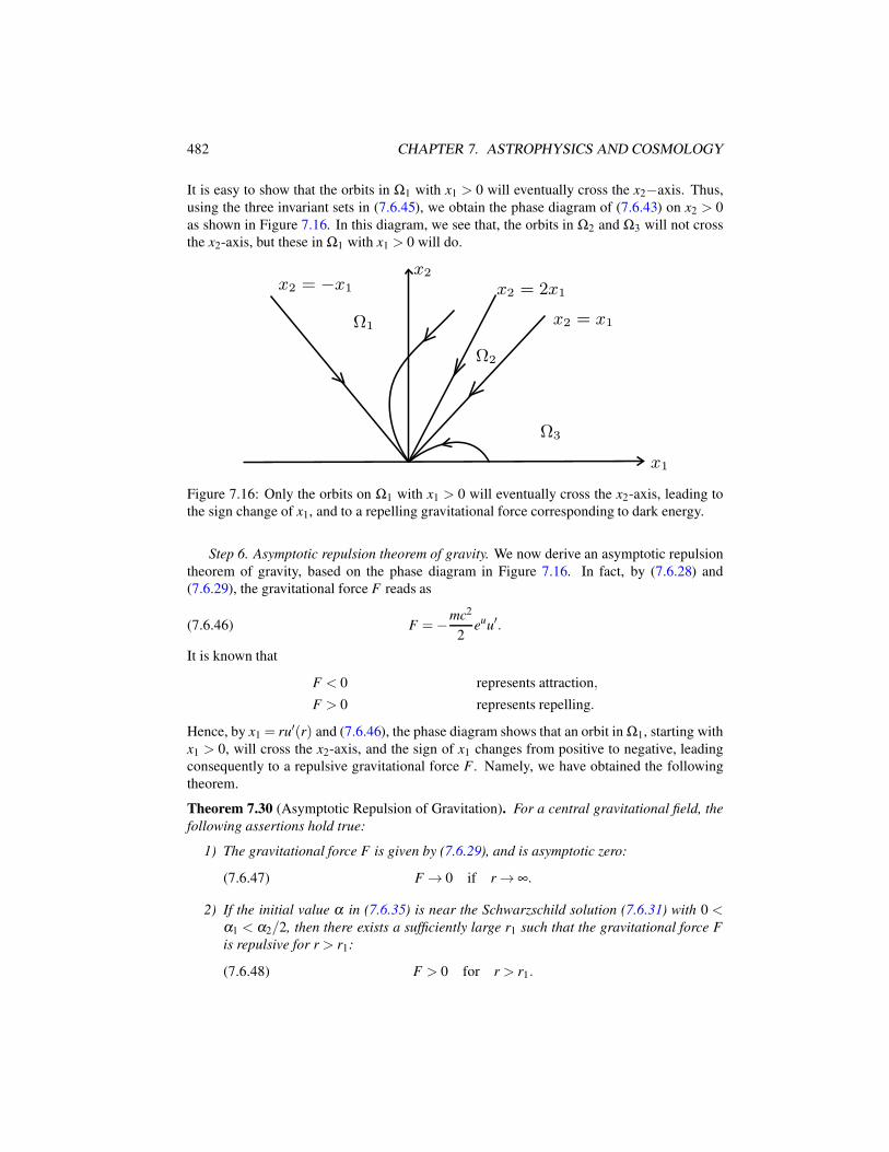
482 CHAPTER 7. ASTROPHYSICS AND COSMOLOGY
It is easy to show that the orbits in Ω1 with x1 > 0 will eventually cross the x2−axis. Thus,
using the three invariant sets in (7.6.45), we obtain the phase diagram of (7.6.43) on x2 > 0
as shown in Figure 7.16. In this diagram, we see that, the orbits in Ω2 and Ω3 will not cross
the x2-axis, but these in Ω1 with x1 > 0 will do.
x1
Ω3
x2 = x1
Ω2
x2 = 2x1
x2
Ω1
x2 = −x1
Figure 7.16: Only the orbits on Ω1 with x1 > 0 will eventually cross the x2-axis, leading to
the sign change of x1, and to a repelling gravitational force corresponding to dark energy.
Step 6. Asymptotic repulsion theorem of gravity. We now derive an asymptotic repulsion
theorem of gravity, based on the phase diagram in Figure 7.16. In fact, by (7.6.28) and
(7.6.29), the gravitational force F reads as
(7.6.46) F =−mc2
2euu′.
It is known that
F < 0 represents attraction,
F > 0 represents repelling.
Hence, by x1 = ru′(r) and (7.6.46), the phase diagram shows that an orbit in Ω1, starting with
x1 > 0, will cross the x2-axis, and the sign of x1 changes from positive to negative, leading
consequently to a repulsive gravitational force F . Namely, we have obtained the following
theorem.
Theorem 7.30 (Asymptotic Repulsion of Gravitation). For a central gravitational field, the
following assertions hold true:
1) The gravitational force F is given by (7.6.29), and is asymptotic zero:
(7.6.47) F → 0 if r → ∞.
2) If the initial value α in (7.6.35) is near the Schwarzschild solution (7.6.31) with 0 <α1 < α2/2, then there exists a sufficiently large r1 such that the gravitational force F
is repulsive for r > r1:
(7.6.48) F > 0 for r > r1.
7.6. THEORY OF DARK MATTER AND DARK ENERGY 483
We remark that Theorem 7.30 is valid provided the initial value α is small because the
diagram given by Figure 7.16 is in a neighborhood of x = 0. However, all physically mean-
ingful central fields satisfy the condition (note that any a black hole is enclosed by a huge
quantity of matter with radius r > 0 ≫ 2MG/c2). In fact, the Schwarzschild initial values are
as
(7.6.49) x1(r0) = x2(r0) =δ
1− δ, δ =
2MG
c2r0.
For example see (7.6.29), where the δ -factors are of the order δ ≤ 10−1, sufficient for the
requirements of Theorem 7.30.
The most important cases are for galaxies and clusters of galaxies. For these two types of
astronomical objects, we have
galaxy : M = 1011M⊙, r0 = 3× 10⁵ly,
cluster of galaxies : M = 1014M⊙, r0 = 3× 10⁶ly.
Thus the δ -factors are
(7.6.50) galaxies δ = 10−7, cluster of galaxies δ = 10−5.
In fact, the dark energy phenomenon is mainly evident between galaxies and between clusters
of galaxies. Hence, (7.6.50) shows that Theorem 7.30 is valid for both central gravitational
fields of galaxies and clusters of galaxies. The asymptotic repulsion of gravity plays the role
to stabilize the large scale homogeneous structure of the Universe.
7.6.5 Simplified gravitational formula
We have shown that all four fundamental interactions are layered. Namely, each interaction
has distinct attracting and repelling behaviors in different scales and levels. The dark matter
and dark energy represent the layered property of gravity.
In this section, we simplify the gravitational formula (7.6.32) to clearly exhibit the layered
phenomena of gravity.
In (7.6.32) the field functions u and v can be approximatively replaced by the Schwarzschild
solution (7.6.30). Since 2MG/c2r is very small for r > r0 as indicted in (7.6.29) and (7.6.50),
the formula (7.6.32) can be expressed as
(7.6.51) F = mMG
[− 1
r2− r
δ r0
φ ′′], r > r0.
By the field equation (7.6.26), we have
(7.6.52) R = Φ for r > r0,
where R is the scalar curvature, and
Φ = gµνDµνφ = e−v
[−φ ′′+
1
2(u′− v′)φ ′+
2
rϕ ′].
484 CHAPTER 7. ASTROPHYSICS AND COSMOLOGY
In view of (7.6.52), we obtain that
φ ′′ =−evR+2
rφ ′+
1
2(u′− v′)φ ′
Again by the Schwarzschild approximation, we have
(7.6.53) φ ′′ =
(2
r+
δ r0
r2
)φ ′−R.
Integrating (7.6.53) and omitting e±δ r0/r, we derive that
φ ′ =−r2
[ε +
∫r−2Rdr
],
where ε is a constant. Thus (7.6.51) can be rewritten as
(7.6.54) F = mMG
[− 1
r2+
r
δ r0
R+
(1+
2r
δ r0
)(εr+ r
∫R
r2dr
)].
The solutions of (7.6.34) can be Taylor expanded. Hence by (7.6.33) we see that
u′(r) =1
r2
∞
∑k=0
ak(r− r0)k.
By (7.6.46), the gravitational force F takes the following form
F =1
r2
∞
∑k=0
bkrk, b0 =−mMG.
In view of (7.6.54), it implies that R can be expanded as
R =ε0
r− ε1 +O(r),
and by Physical Conclusion 7.29, ε0 and ε1 are two to-be-determined free parameters. Insert-
ing R into (7.6.54) we obtain that
(7.6.55) F = mMG
[− 1
r2− k0
r+ϕ(r)
]for r > r0.
where k0 =12ε0, and
ϕ(r) = ε1 + k1r+O(r), k1 = ε +ε1
δ r0
.
The nature of dark matter and dark energy suggests that
k0 > 0, k1 > 0.
Based on Theorem 7.30, ϕ(r)→ 0 as r → ∞, and (7.6.55) can be further simplified as in the
form for r0 < r < r1,
(7.6.56) F = mMG
[− 1
r2− k0
r+ k1r
],
7.6. THEORY OF DARK MATTER AND DARK ENERGY 485
where k0 and k1 will be determined by the Rubin rotational curve and the astronomical data
for clusters of galaxies in the next section, where we obtain that
(7.6.57) k0 = 4× 10⁻¹⁸km−2, k1 = 10−57km−3.
The formula (7.6.56) is valid only in the interval
r0 < r < r1,
and r1 is the distance at which F changes its sign:
F(r1) = 0.
Both observational evidence on dark energy and Theorem 7.30 show that the distance r1
exists. The formula (7.6.56) with (7.6.57) clearly displays the layered property of gravity:
attracting at short distance and repelling at large distance.
7.6.6 Nature of dark matter and dark energy
As mentioned in Section 7.6.2, both dark matter and dark energy are a property of gravita-
tional effect, reflected in two aspects, which will be addressed in detail in this section:
a) spatially geometrical structure, and
b) gravitational attracting and repelling as in (7.6.56).
Space curved energy and negative pressure
Gravitational potential causes space curvature and the spherical structure of the Universe,
and displays two types of energies: a) dark matter contributed by the curvature of space, and
b) dark energy generated by the dual gravitational potential in (7.6.17). We address each type
of energy as follows.
1. Dark matter: the space curved energy. In Section 7.5.2, we have introduced the space
curved energy Mtotal for the 3D spherical Universe as follows:
Mtotal =3π
2M, M is the observed mass in the hemisphere.
Now, we consider a galaxy with an observed mass MΩ. By (7.5.51), we have shown that the
space curved energy Mtotal;Ω is
(7.6.58) Mtotal;Ω =VΩ
|Ω|MΩ,
where Ω is the domain occupied by the galaxy, VΩ and |Ω| are the volumes of curved and flat
Ω. VΩ contain two parts:
(7.6.59) VΩ = cosmic spherical V 1Ω + local bump V 2
Ω.
486 CHAPTER 7. ASTROPHYSICS AND COSMOLOGY
It is known that
V 1Ω =
3π
4|Ω|.
For V 2Ω, we propose that
V 2Ω = π2r3
0, r0 the galaxy radius.
In fact, the formula is precise for the galaxy nucleus.
By |Ω|= 43πr3
0 , we infer from (7.6.58) and (7.6.59) that
(7.6.60) Mtotal;Ω =3π
2MΩ,
which gives rise to the relation between the masses of dark matter and observable matter.
2. Dark energy: the dual gravitational potential. The static universe is described by the
stationary solution of (7.6.13)-(7.6.14), which is given by (7.6.15)-(7.6.16). In the solution
a negative pressure presents, which prevents galaxies and clusters of galaxies from gravita-
tional contraction to form a void universe, and maintains the homogeneous distribution of the
Universe. The negative pressure contains two parts:
(7.6.61) p =−1
3ρc2 − c2
24πGϕ (see (7.6.15)),
where the first term is contributed by the observable energy, and the second term is the dark
energy generated by the dual gravitational potential ϕ ; see also (7.6.21).
By the Blackhole Theorem, Theorem 7.15, black holes are incompressible in their interi-
ors. Hence, in (7.6.61) the negative pressure
(7.6.62) p =−1
3ρc2,
is essentially the incompressible pressure of the black hole generated by the normal energy.
By the cosmology theorem, Theorem 7.27, the Universe is a 3D sphere with a blackhole
radius. However, the CMB and the WMAP measurements manifest that the cosmic radius
R is greater than the blackhole radius of normal energy. By (7.6.21), the deficient energy is
compensated by the dual gravitational potential, i.e. by the second term of (7.6.61).
Attraction and repulsion of gravity
Based on Theorem 7.30, gravity possesses additional attraction and repelling to the New-
tonian gravity, as shown in the revised gravitational formula:
(7.6.63) F = mMG
(− 1
r2− k0
r+ k1r
).
By using this formula we can explain the dark matter and dark energy phenomena. In par-
ticular, based on the Rubin rotational curve and astronomical data, we can determine an
approximation of the parameters k0 and k1 in (7.6.63).
7.6. THEORY OF DARK MATTER AND DARK ENERGY 487
1. Dark matter: the additional attraction. Let Mr be the total mass in the ball with radius
r of galaxy, and V be the constant galactic rotational velocity. By the force equilibrium, we
infer from (7.6.63) that
(7.6.64)V 2
r= MrG
(1
r2+
k0
r− k1r
),
which implies that
(7.6.65) Mr =V 2
G
r
1+ k0r− k1r3.
The mass distribution (7.6.65) is derived based on both the Rubin rotational curve and the
revised formula (7.6.63). In the following we show that the mass distribution Mr fits the
observed data.
We know that the theoretic rotational curve given by Figure 7.15 (b) is derived by using
the observed mass Mob and the Newton formula
F =−mMobG
r2.
Hence, to show that Mr =Mob, we only need to calculate the rotational curve vr by the Newton
formula from the mass Mr, and to verify that vr is consistent with the theoretic curve. To this
end, we havev2
r
r=
MrG
r2,
which, by (7.6.65), leads to
vr =V√
1− k0r− k1r2.
As k1 ≪ k0 ≪ 1,vr can be approximatively written as
(7.6.66) vr =V (1− 1
2k0r+
1
4k2
0r2).
It is clear that the rotational curve described by (7.6.66) is consistent with the theoretic rota-
tional curve as illustrated by Figure 7.15 (b). Therefore, it implies that
(7.6.67) Mr = Mob.
The facts of (7.6.64) and (7.6.67) are strong evidence to show that the revised formula
(7.6.63) is in agreement with the astronomical observations.
We now determine the constant k0 in (7.6.63). According to astronomical data, the aver-
age mass Mr1and radius r1 of galaxies are about
(7.6.68)Mr1
= 1011M⊙ ∼= 2× 1041Kg,
r1 = 104 ∼ 105pc ∼= 1018Km.
The observations show that the constant velocity V in the Rubin rotational curve is about
V = 300km/s. Then we have
V 2
G= 1024kg/km
488 CHAPTER 7. ASTROPHYSICS AND COSMOLOGY
Based on physical considerations,
(7.6.69) k0 ≫ k1r1 (r1 as in (7.6.68)).
Then, we deduce from (7.6.65) that
(7.6.70) k0 =V 2
G
1
Mr1
− 1
r1
= 4× 10⁻¹⁸K−1m .
We can explain the dark matter by the revised formula (7.6.63). As the matter distribution
Mr is in the form
Mr =V 2
G
r
1+ k0r,
then the Rubin law holds true. In addition, the revised gravitation produces an excessive mass
M as
M = MT −Mr1=
V 2
Gr1 −
V 2
G
r1
1+ k0r1
,
where M1 =V 2r1/G is the Newton theoretic value of the total mass. Hence we have
M
MT
=k0r1
1+ k0r1
=4
5or
M
Mr1
= 5.
Namely, the additional mass M is four time the visible matter Mr1= MT − M. Thus, it gives
an explanation for the dark matter.
We remark that the ratio M/Mob = 5 is essentially the same as in (7.6.60). It shows that
the dark matter is a gravitational effect, reflected in both the space curvature and the additional
gravitational attraction.
2. Dark energy: asymptotic repulsion of gravity. If gravity is always attracting as given
by the Newton formula, then the cosmic homogeneity is unstable. In fact, It is known that the
average mass M and distance for the clusters of galaxies are as
(7.6.71)M = 1014M⊙ ∼= 1044Kg
r ∼= 108pc ∼= 1020 ∼ 1021Km.
Then the Newton gravitation between two clusters of galaxies is
(7.6.72) F =−M2G
r2∼= 1029N = 1028Kg.
However, astronomical observations indicate that no gravitational interaction between
clusters of galaxies. The Universe is isotropic, therefore no rotation to balance the huge force
of (7.6.72) in the clusters.
Thus, the new cosmology theorem, Theorem 7.27, suggests that gravity should be asymp-
totically repulsive. Theorem 7.30 offers a solid theoretic foundation for the property, based
on which we derive the simplified gravitational force formula (7.6.63).
7.6. THEORY OF DARK MATTER AND DARK ENERGY 489
Now we consider the constant k1 in (7.6.63). Due to the astronomical fact that no gravi-
tational force between clusters of galaxies, we have
F(r) = 0, r = the average distance between galactic clusters.
By (7.6.71), we take
(7.6.73) r =
√2
5× 10²⁰km.
Then we deduce from (7.6.63) that
k1r− k0
r− 1
r2= 0,
which, by (7.6.70) and (7.6.73), leads to
(7.6.74) k1 = 10−57km−3.
In summary, we conclude that the dark matter and dark energy are essentially gravitational
effect generated by the gravitational potential field gµν , its dual field Φµ and their nonlinear
interactions. They can be regarded as the gravitational field energy caused by gµν and Φµ .

490 CHAPTER 7. ASTROPHYSICS AND COSMOLOGY
Bibliography
Davis, R., Harmer, D. S., and Hoffman, K. C. (1968). Search for neutrinos from the sun,
Phys. Rev. Lett. 20, pp. 1205–1209, doi:10.1103/PhysRevLett.20.1205.
de Broglie, L. (1924). Recherches sur la theorie des quanta, Thesis Paris.
Einstein, A. (1905). Uber einen die Erzeugung und Verwandlung des Lichtes betreffenden
heuristischen Gesichtspunkt, Annalen der Physik 322, pp. 132–148, doi:10.1002/andp.
19053220607.
Einstein, A. (1915). Die feldgleichungen der gravitation, Sitzungsberichte der Preussischen
Akademie der Wissenschaften zu Berlin , pp. 844–847.
Einstein, A. (1916). The foundation of the general theory of relativity, Annalen der Physik
354 (7), pp. 769–822.
Englert, F. and Brout, R. (1964). Broken symmetry and the mass of gauge vector mesons,
Physical Review Letters 13 (9), p. 32123.
Greiner, W. (2000). Relativistic quantum mechanics, .
Griffiths, D. (2008). Introduction to elementary particles (Wiley-Vch).
Gross, D. J. and Wilczek, F. (1973). Ultraviolet behavior of non-abelian gauge theories, Phys.
Rev. Lett. 30, pp. 1343–1346, doi:10.1103/PhysRevLett.30.1343.
Guralnik, G., Hagen, C. R., and Kibble, T. W. B. (1964). Global conservation laws and mass-
less particles, Physical Review Letters 13 (20), p. 585587.
Halzen, F. and Martin, A. D. (1984). Quarks and leptons: an introductory course in modern
particle physics (John Wiley and Sons, New York, NY).
Harrison, E. (2000). Cosmology, the science of the universe, 2nd edn. (Cambridge University
Press).
Hernandez, M., Ma, T., and Wang, S. (2015). Theory of dark energy and dark matter, .
Higgs, P. W. (1964). Broken symmetries and the masses of gauge bosons, Physical Review
Letters 13, p. 508509.
Kaku, M. (1993). Quantum Field Theory, A Modern Introduction (Oxford University Press).
491
492 BIBLIOGRAPHY
Kane, G. (1987). Modern elementary particle physics, Vol. 2 (Addison-Wesley Reading).
Klein, O. (1938). New Theories in Physics, 77 (Intern. Inst. of Intellectural Co-operation,
League of nations).
Kutner, M. L. (2003). Astronomy: A Physical Perspective (Cambridge University Press).
Landau, L. (1957). On the conservation laws for weak interactions, Nuclear Physics 3, 1, pp.
127 – 131, doi:http://dx.doi.org/10.1016/0029-5582(57)90061-5.
Landau, L. D. and Lifshitz, E. M. (1975). Course of theoretical physics, Vol. 2, 4th edn.
(Pergamon Press, Oxford), the classical theory of fields, Translated from the Russian by
Morton Hamermesh.
Lee, T. D. and Yang, C. N. (1956). Question of parity conservation in weak interactions, Phys.
Rev. 104, pp. 254–258, doi:10.1103/PhysRev.104.254.
Lee, T. D. and Yang, C. N. (1957). Parity nonconservation and a two-component theory of
the neutrino, Phys. Rev. 105, p. 1671.
Ma, T. (2010). Manifold Topology (Science Press, Beijing (in Chinese)).
Ma, T. (2011). Theory and Methods of Partial Differential Equations (Science Press, Beijing
(in Chinese)).
Ma, T. (2012). Physical World From the Mathematical Point of View: Geometrical Analysis,
Gravitational Field, and Relativity (Science Press, Beijing (in Chinese)).
Ma, T. (2014). Physical World From the Mathematical Point of View: Theory of Elementary
Particles and Unified Fields (Science Press, Beijing (in Chinese)).
Ma, T. and Wang, S. (2005). Bifurcation theory and applications, World Scientific Series on
Nonlinear Science. Series A: Monographs and Treatises, Vol. 53 (World Scientific Pub-
lishing Co. Pte. Ltd., Hackensack, NJ), ISBN 981-256-287-7.
Ma, T. and Wang, S. (2013a). Duality theory of weak interaction, IU ISCAM Preprint Series,
#1302: http://www.indiana.edu/~iscam/preprint/1302.pdf.
Ma, T. and Wang, S. (2013b). Phase Transition Dynamics (Springer-Verlag).
Ma, T. and Wang, S. (2013c). Structure and stability of matter, IU ISCAM Preprint Series,
#1303: http://www.indiana.edu/~iscam/preprint/1303.pdf.
Ma, T. and Wang, S. (2014a). Astrophysical dynamics and cosmology, Journal of Mathemat-
ical Study 47:4, pp. 305–378.
Ma, T. and Wang, S. (2014b). Color algebra in quantum chro-
modynamics, Isaac Newton Institute Preprint # NI14001:
https://www.newton.ac.uk/files/preprints/ni14001.pdf.
BIBLIOGRAPHY 493
Ma, T. and Wang, S. (2014c). Duality theory of strong interaction, Electronic Jour-
nal of Theoretical Physics 11:31, pp. 101–124, iU ISCAM Preprint Series, #1301:
http://www.indiana.edu/~iscam/preprint/1301.pdf.
Ma, T. and Wang, S. (2014d). Field theory for multi-particle system, Isaac Newton Institute
Preprint # NI14057: https://www.newton.ac.uk/files/preprints/ni14057.pdf.
Ma, T. and Wang, S. (2014e). Gravitational field equations and theory of dark matter and dark
energy, Discrete and Continuous Dynamical Systems, Ser. A 34:2, pp. 335–366, preprint,
http://arxiv.org/abs/1206.5078.
Ma, T. and Wang, S. (2014f). On solar neutrino problem, Isaac Newton Institute Preprint #
NI14058: https://www.newton.ac.uk/files/preprints/ni14058.pdf.
Ma, T. and Wang, S. (2014g). Spectral theory of differential operators and en-
ergy levels of subatomic particles, Isaac Newton Institute Preprint # NI14002:
https://www.newton.ac.uk/files/preprints/ni14002.pdf.
Ma, T. and Wang, S. (2014h). Unified field theory and principle of representation
invariance, Applied Mathematics and Optimization 69:3, pp. 359–392, doi:0.1007/
s00245-013-9226-0, preprint, http://arxiv.org/abs/1212.4893.
Ma, T. and Wang, S. (2015a). Unified field equations coupling four forces and principle of
interaction dynamics, Discrete and Continuous Dynamical Systems, Ser. A 35:3, pp. 1103–
1138, preprint, http://arxiv.org/abs/1210.0448.
Ma, T. and Wang, S. (2015b). Weakton model of elementary particles and decay mechanisms,
Electronic Journal of Theoretical Physics 12:32, pp. 139–178, iU ISCAM Preprint Series,
#1304: http://www.indiana.edu/~iscam/preprint/1304.pdf.
Maki, Z., Nakagawa, M., and Sakata, S. (1962). Remarks on the unified model of elementary
particles, Progress of Theoretical Physics 28, pp. 870–880.
Mikheev, S. P. and Smirnov, A. Y. (1986). Resonant amplification of ν oscillation in matter
and solar-neutrino spectroscopy, IL Nuovo Cimento C 9:1, pp. 17–26.
Milgrom, M. (1983). A modification of the Newtonian dynamics as a possible alternative to
the hidden mass hypothesis, Astrophysical Journal 270, pp. 365–370, doi:10.1086/161130.
Milgrom, M. (2014). MOND laws of galactic dynamics, MNRAS 437, pp. 2531–2541, doi:
10.1093/mnras/stt2066, eprint 1212.2568.
Nambu, Y. (1960). Quasi-particles and gauge invariance in the theory of superconductivity,
Phys. Rev. 117, pp. 648–663, doi:10.1103/PhysRev.117.648.
Nambu, Y. (2008). Spontaneous symmetry breaking in particle physics: a case of cross fer-
tilization, Slides for his Nobel Lecture.
Nambu, Y. and Jona-Lasinio, G. (1961a). Dynamical model of elementary particles based on
an analogy with superconductivity. I, Phys. Rev. 122, pp. 345–358, doi:10.1103/PhysRev.
122.345.
494 BIBLIOGRAPHY
Nambu, Y. and Jona-Lasinio, G. (1961b). Dynamical model of elementary particles based on
an analogy with superconductivity. II, Phys. Rev. 124, pp. 246–254, doi:10.1103/PhysRev.
124.246.
Perlmutter, S. and et al. (1999). Measurements of ω and λ from 42 high-redshift supernovae,
Astrophys. J. 517, pp. 565–586.
Planck, M. (1901). Ueber das Gesetz der Energieverteilung im Normalspectrum, Annalen der
Physik 309, pp. 553–563, doi:10.1002/andp.19013090310.
Politzer, H. D. (1973). Reliable perturbative results for strong interactions? Phys. Rev. Lett.
30, pp. 1346–1349, doi:10.1103/PhysRevLett.30.1346.
Pontecorvo, B. (1957). Mesonium and anti-mesonium, Sov.Phys.JETP 6, p. 429.
Pontecorvo, B. (1968). Neutrino experiments and the problem of conservation of leptonic
charge, Sov.Phys.JETP 26, p. 984.
Popławski, N. (2012). Nonsingular, big-bounce cosmology from spinor-torsion coupling,
Phys. Rev. D 85, p. 107502, doi:10.1103/PhysRevD.85.107502.
Quigg, C. (2013). Gauge theories of the strong, weak, and electromagnetic interactions, 2nd
edition (Princeton Unversity Press).
Riess, A. G. and et al. (1989). Observational evidence from supernovae for an accelerating
universe and a cosmological constant, Astron. J. 116, pp. 1009–1038.
Roos, M. (2003). Introduction to Cosmology, Third Edition (Wiley).
Rubin, V. and Ford, J. W. K. (1970). Rotation of the andromeda nebula from a spectroscopic
survey of emission regions, Astrophysical Journal 159, pp. 379–404.
Sakurai, J. J. (1994). Modern Quantum Mechanics, revised edn. (Addison-Wesley Publishing
Company, Inc.).
Salam, A. (1957). On parity conservation and neutrino mass, Nuovo Cimento 5, pp. 299–301.
Sokolov, A. A., Loskutov, Y. M., and Ternov, I. M. (1966). Quantum Mechanics (Holt, Rine-
hart abd Winston, Inc.).
Weisskopf, V. (1972). Physics in the Twentieth Century: Selected Essays (Cambridge, Mas-
sachusetts: MIT Press).
Weyl, H. (1912). Das asymptotische Verteilungsgesetz der Eigenwerte linearer partieller
Differentialgleichungen (mit einer Anwendung auf die Theorie der Hohlraumstrahlung),
Math. Ann. 71, 4, pp. 441–479, doi:10.1007/BF01456804.
Weyl, H. (1919). Raum, Zeit, Materie (Verlag von Julius Springer).
Weyl, H. (1929). Electron and gravitation, Z. Phys. 56, pp. 330–352.
BIBLIOGRAPHY 495
Wolfenstein, L. (1978). Neutrino oscillations in matter, Phys. Rev. D 17, pp. 2369–2374,
doi:10.1103/PhysRevD.17.2369.
Wu, C. S., Ambler, E., Hayward, R. W., Hoppes, D. D., and Hudson, R. P. (1957). Ex-
perimental test of parity conservation in beta decay, Phys. Rev. 105, pp. 1413–1415, doi:
10.1103/PhysRev.105.1413.
Yang, C. N. and Mills, R. (1954). Conservation of isotopic spin and isotopic gauge invariance,
Physical Review 96, pp. 191–195.
Zwicky, F. (1937). On the masses of nebulae and of clusters of nebulae, Astrophysical Journal
86, pp. 217–246.

496 BIBLIOGRAPHY
Index
Symbols
D0-decay, 307
De, gradient operator, 202
Dg, gradient operator, 202
Ds, gradient operator, 202
Dw, gradient operator, 202
G-parity, 260
Hk Sobolev space, 125
Lp spaces, 123
SU(N), 269
SU(N) gauge transformation, 118
SU(N) representation, 73
SU(N) representation invariance, 156
SU(N) tensor, 161
Sn, n-sphere, 108
TM = M ⊗p TpM , tangent bundle, 113
U(1) gauge invariance, 70
W± bosons, 211
W k,p Sobolev space, 124
Z boson, 211
∆++-decay, 306
Gab(A), SU(N) tensor, 161
Γrkl , Levi-Civita connection, 147
M ⊗p EN , vector bundle, 113
β -decay, 261, 305
δ -factor, 436, 438
λk, Gell-Mann matrices, 163, 204
M ⊗p Cn, complex bundle, 11
ν-mediator, 295
ρw, radius of w∗-weakton, 219
σk, Pauli matrices, 163, 204
M ,gµν, Riemannian manifold, 11
e, the negative electric charge, 57, 180
f abc, structure constants for Gell-Mann
Matrices, 163
gs, strong charge, 180
gw, weak charge, 180
mH , mass of φw, 205
mπ , mass of φ s, 205
ml , 201
mq, 201
ms, 202
mw, 202
w∗-color algebra, 320
4-D gradient operator, 51
m⊙, solar mass, 412
A
accretion, 454
active galaxy, 443
AGN, 451
angular momentum conservation, 265
angular momentum rule, 342, 344
arc-length, 111
Archytas, 463
astrophysical fluid dynamics, 396, 408
asymptotic flatness, 479
asymptotic freedom, 227
atomic spectrum, 389
B
baryon, 256
spectral equations, 370
baryon decay, 263
baryon number, 259
497
498 INDEX
BEC
Bose-Einstein condensation, 104
Betti number, 141
Bianchi identity, 192, 474
Big-Bang, 457
black hole, 402
existence of, 402
black holes, 432
geometric realization, 432
Blackhole Theorem, 395, 434
Bohr atomic model, 166
Bose-Einstein condensation
Hamiltonian system for, 104
boson, 254
bound state, 367
bremsstrahlung, 310
mechanism of, 310
C
Chandrasekhar limit, 436
charged Higgs, 211
charged lepton, 366
mediator cloud, 324
weakton constituent, 294
CKM matrix, 352
classical electrodynamics, 82
cluster of galaxies, 412
CMB problem, 465
color algebra, 316, 317
color charge, 314
color index, 315, 317
formula for hadron, 318
color quantum number, 311
conjugate representation, 272
connection, 119
for GL(n) group, 121
for SU(N) group, 120
for Lorentz group, 120
conservation
of weakton number, 302
conservation laws, 89, 264
conservative systems
dynamics of, 96
control parameter, 418
cosmic edge problem, 463
cosmic radius, 466
cosmological constant, 70
Cosmology Theorem, 470
Coulomb potential, 207
covariant derivative, 63, 65, 66
on a vector bundle, 119
critical δ -factor, 438
current density, 51
curvature tensor, 67
D
dark energy, 23, 24, 192, 471, 473
theory of, 476
dark matter, 23, 24, 192, 471
dark matter and dark energy
the nature of, 485
de Broglie relation, 57
decay, 261, 304
decay type, 303
decoupling
of the unified field theory, 209
deep inelastic scattering, 227
derivative on TM , 121
derivative on T ∗M , 121
derivative on T kr M , 122
differential operators, 128
in spherical coordinates, 403
Dirac equations, 45, 57, 336
Hamiltonian system for, 103
Dirac matrices, 58, 334
Dirac spinor, 58
Dirac spinor fields, 87
dissipative systems, 418
divergence operator, 129, 397, 405
dual gluon, 313
dual gluons, 211, 216
dual gravitational potential, 486
dual graviton, 211, 212
dual photon, 211, 214
duality
for the weak interaction, 218
of field particles, 210
of interacting forces, 211
of mediators, 210
duality of fundamental interactions, 209
INDEX 499
dynamic transition theory, 418, 450
classification, 419
E
Eotvos, 63
Eddington coordinate transformation, 434
Eightfold Way, 267
Einstein energymomentum relation, 56
Einstein equation
non-well-posedness of, 193
Einstein equations
non well-posedness, 194
Einstein gravitational field equations, 35,
68, 398, 400, 429
Einstein mass-energy formula, 53
Einstein’s theory of general relativity, 60
Einstein-Hilbert action, 67
Einstein-Hilbert functional, 67, 68
derivative operator, 147
elastic scatterring, 227
elastic waves, 81
electric charge, 180, 257
electric field, 54
electromagnetic force, 180, 215
electromagnetic potential, 50, 407
electromagnetism, 14, 181
electron degeneracy pressure, 436
electron structure, 309
electron-positron pair
creation and annihilation, 300
electroweak theory, 244
problems in, 249
elementary particle
strong interaction potential of, 218
elliptic operator
negative eigenvalues of, 169
elliptical galaxy, 442, 446
energy conservation, 264, 303
energy level, 358, 367
energy levels, 166
energy operator, 333
energy rule, 303
energy spectrum, 371
discreteness, 373
energy-momentum conservation,
406, 407
energy-momentum tensor, 400
of idealized fluid, 400
energy-momentum vector, 51
equation of state, 406, 408, 428
essence of physics, 34
expansion of the Universe, 456
F
fermion, 254
field equations
for the strong interaction, 216
for the weak interaction, 217
field theory
multi-particle system, 377
first Betti number, 141
flatness problem, 463
fluid dynamic equations, 396, 407
momentum representation of, 406
four forces, 180
four interactions, 180
Fredholm Alternative Theorem, 133
Friedmann cosmology, 459
fundamental representation, 271
G
G-parity, 260
G. Lemaıtre, 457
galaxies, 442
galaxy, 412
galaxy cluster, 445
galaxy types, 442
Galilean invariance, 44
gauge invariance, 44, 70, 78
gauge symmetry
physical implication of, 188
gauge symmetry breaking, 188
principle of, 189
gauge transformation, 118
SU(2), 187
gauge-fixing problem, 208
non well-posedness of, 209
Gauss formula, 131, 132
500 INDEX
Gell-Mann matrices, 163
Gell-Mann-Zweig
quark model, 284
general invariants, 64
general tensor, 63
generator representation
of SU(N), 72
geometric interaction mechanism, 182
geometry of unified fields, 185
Ginzburg-Landau free energy, 199
globular universe, 462
gluon, 312, 313
gluon radiation, 314
color transformation, 319
gluons, 211, 216
gradient operator, 129, 405
gravitational field equations, 68, 406, 425
based on PID, 211
gravitational force, 180, 212
gravitational force formula, 212
gravitational interaction formula, 477,
483
gravitational mass, 63
gravitational potential, 45, 407
graviton, 211, 212
gravity, 181
asymptotic repulsion, 478
guiding principle
of theoretical physics, 34
H
Holder space, 125
hadron, 254, 256, 283, 326
gluon cloud, 326
Hamiltonian dynamics, 80, 97
Hamiltonian system
energy-conservation of, 98
for Bose-Einstein condensation, 104
for Dirac equations, 103
for Klein-Gordon equation, 104
for Schrodinger equation, 102
for Weyl equations, 102
Hamiltonian systems
in classical mechanics, 93
heat conduction, 407
Heisenberg uncertainty relation, 340
Helmholtz decomposition, 135
Higgs mechanism, 196
Hodge theory, 142
Homestake experiments, 348
horizon problem, 463
Hubble, 443
Hubble Law, 456
hypercharge, 260
I
Indc, color index, 317
inertial mass, 63
interaction potential pressure, 437
irreducible representation, 269
computation, 278
of SU(N), 273
isospin, 260
J
Jeans theory, 440
jets, 451, 454
K
KamLAND, 349
KG equation, 56
Klein-Gordon equation, 56, 335
Hamiltonian system for, 104
Klein-Gordon fields, 87
Kruskal coordinate transformation, 434
L
Lagrangian action, 68
Lagrangian actions
in quantum mechanics, 86
Lagrangian dynamics, 80
Lagrangian for dynamics of charged
particles, 84
Laplace operator, 130
Laplace-Beltrami operator, 131, 396, 404
latitudinal circulation, 454
Lemaıtre cosmology, 460
lepton, 254
lepton decay, 262, 306
lepton numbers, 258
INDEX 501
Leray decomposition, 136
Levi-Civita connection, 62, 147, 396
Lie group, 270
irreducible representation, 270
lifetime, 257
linear elliptic equation, 133
linear hyperbolic equation, 134
Lipschitz space, 125
Lorentz force, 207
Lorentz invariance, 44, 46
Lorentz invariants, 51
Lorentz tensor, 47, 50
Lorentz transformation, 46
Lorentz transformation group, 49
M
magnetic field, 54
magnetic potential, 207
main driving force, 414
pressure gradient, 415
relativistic effect, 415
stellar dynamics, 414
thermal expansion force, 415
viscous friction, 415
main-sequence stars, 413, 420
manifold with boundary, 143
mass, 257
mass charge, 180
mass generation, 196, 295
mass of earth’s black hole core, 442
mass of solar black hole core, 441
massive bound state, 362
massless bound state, 364
Maxwell equations, 214
modified, 214
Maxwell equations for electromagnetic
fields, 54
mechanism of supernova explosion, 429
mediator, 254, 255
energy spectrum, 371
weakton constituents, 294
mediator cloud, 311, 324
of quark, 325
structure of, 311
mediator decay, 263
meson, 256
spectral equations, 370
meson decay, 264
Milky Way galaxy, 444
Minkowski space, 47
mixed decay, 308
mixed type decay, 304
mixing matrix, 352
MNS matrix, 352
modified QED model, 213
modified Yukawa potential, 228
momentum conservation, 265
momentum operator, 333
MSW effect, 354
multi-particle system, 377
N
Navier-Stokes equations, 396
in spherical coordinates, 405
negative pressure, 466, 485
neutral Higgs, 211
neutrino
non-oscillation mechanism, 357
neutrino mass, 352
neutrino oscillation, 350
neutron degeneracy pressure, 436
neutron star and pulsar, 414, 421
Newton cosmology, 458
Newtonian dynamics, 80
Newtonian Gravitational Law, 35
Newtonian gravitational potential, 398
Newtonian Second Law, 406
Noether Theorem, 90
O
observable, 332
Oort, J., 472
Oppenheimer limit, 436
origin of stars and galaxies, 439
Orthogonal Decomposition Theorem
for tensor fields, 136
P
parity, 259
502 INDEX
parity problem, 355
particle decay, 261
particle radiation, 262
particle scattering, 261
particle transition, 260
Pauli exclusion principle, 311, 340, 342
Pauli matrices, 163
Penzias, A., 465
PHD
abbreviation for principle of
Hamiltonian dynamics, 93
for electrodynamics, 100
photon, 211
PID
principle of interaction dynamics, 44
PID cosmological model, 473
PID field equations, 190
PID gravitational field equations, 211
PID gravitational interaction formula,
477
PLD, 208
abbreviation for Principle of
Lagrangian Dynamics, 79
principle of Lagrangian dynamics,
36
quantum dynamics, 337
position operator, 333
position vector, 50
Prandtl number, 419
pressure gradient, 415
PRI
abbreviation of principle of
representation invariance, 165
abbreviation for principle of
representation invariance, 191
principle of equivalence, 36, 61, 62
principle of gauge invariance, 78
principle of general relativity, 36, 44, 60
principle of Hamiltonian dynamics
abbreviated as PHD, 93
principle of interaction dynamics, 190
abbreviated as PID, 44
Principle of Lagrangian Dynamics, 37,
79
abbreviated asPLD, 79
principle of Lagrangian dynamics, 208
abbreviated as PLD, 36
principle of Lorentz invariance, 46
principle of representation invariance,
191
abbreviated as PRI, 165
principle of symmetry-breaking, 44, 45
proper distance, 432
proper time, 432
Q
QCD, 216, 227, 312
QED, 213
quantum chromodynamics, 216
quantum Hamiltonian system, 101
quantum mechanics
Lagrangian actions, 86
quantum physics, 332
quantum system, 332
quark, 254, 255, 366
mediator cloud, 325
weakton constituents, 294
quark confinement, 226
quark decay, 263
quark model, 267, 284
quark pari creation, 305
R
radiation, 262
radio-galaxy, 443
radius of earth’s black hole core, 442
radius of solar black hole core, 442
Rayleigh number, 451
Rayleigh-Benard convection, 451
Rayleigh-Benard instability, 453
Rayleign-Benard convection, 409
red giant, 414, 421
redshift problem, 463
relativistic effect, 415
relativistic invariants, 51
relativistic mechanics, 52
relativistic quantum mechanics, 56
basic postulates, 56
representation invariance, 156
INDEX 503
of gauge theory, 165
representation transformation
SU(2), 188
SU(3), 188
Ricci curvature, 396
Ricci curvature tensor, 147
Ricci tensor, 67
Riemannian geometry, 109
Riemannian manifold, 11, 108, 396
Riemannian metric, 109, 110
Rubin rotational curve, 471
S
Sakata model
of hadrons, 283
Sakata’s explanation, 277
scalar curvature, 68
scalar gluons, 216
scalar photon, 314
scalar potential theorem, 154
scattering, 261, 304
Schrodinger equation, 86, 335
Hamiltonian system for, 102
Schwarzschild metric, 397, 400, 432
Schwarzschild solution, 36
Seyfert galaxy, 443
Sobolev embedding theorem, 126
Sobolev space of tensor fields, 123
solar neutrino problem, 346
solar neutrinos
discrepancy of, 346
space curved energy, 485
spectral equations
baryon, 370
meson, 370
Spectral Theorem of Elliptic Operators,
168
spectral theory, 166
spherical universe, 466
spherically symmetric gravitational field,
397
spin, 258
spin operator, 333
spinor transformation, 118
spiral galaxy, 445, 448
spontaneous gauge symmetry breaking,
45
spontaneous symmetry-breaking
PID mechanism of, 241
stable manifold, 480
star, 412
luminosity of, 412
mass of, 412
parameter relation of, 412
radius of, 412
surface temperature of, 412
starburst, 443
stellar atmosphere, 408
stellar atmospheric circulation, 422
stellar cluster, 412
stellar dynamics, 414
main driving force for, 414
stellar interior circulation, 418
strange number, 260
strong charge, 180
strong decay, 306
strong force, 180, 219
strong force potential, 207
strong interacting decay, 303
strong interaction, 14, 182
bound energy, 226
field equations for the, 216
short-range nature of, 233
strong interaction potential, 219
layered formula of, 223
strong interaction potentials, 218
strong magnetic potential, 207
subatomic particle
energy level, 358
mediator cloud, 324
Sudbury Neutrino Observatory, 349
Super-K experiment, 349
superconductivity, 199
supernova, 414, 429
symmetry-breaking, 45
T
tangent bundle, 113
tangent space, 112
Taylor instability, 452
504 INDEX
the Universe
age of, 457
geometric structure of, 458
topological structure, 458
theory of dark matter and dark energy,
471
thermal expansion force, 415
TOV metric, 397, 400, 403
U
unification
the Einstein, 183
based on PID, PRI and PSB, 184
unified field model, 200
coupling matter fields, 385
unified field theory, 179
decoupling of the, 209
V
variable star, 413
variation with divA-free constraint, 144,
150, 152
variational principle, 144
vector bundle, 113
connection on a, 119
covariant derivative on a, 119
linear transformations on, 116
vector photon, 314
Vierbein tensor, 188
viscous friction, 415
W
wave function, 332
weak charge, 180
weak decay, 304
weak force, 180, 218, 234
layered formulas, 236
weak force potential, 207
weak interacting decay, 303
weak interaction, 14, 181
duality of the, 218
field equations for the, 217
theory, 234
weak interaction potential, 234
weak magnetic potential, 207
weak solution, 133
weakly differentiable functions, 123
weakton black hole, 439
weakton color algebra, 320
weakton confinement, 295
weakton constituents, 294
weakton exchange
between leptons and mediators, 301
between quarks and mediators, 302
in mediators, 300
weakton interaction potential, 437
weakton model, 287
weakton number, 302
Weyl asymptotic relation, 171
Weyl equations, 57, 335
Hamiltonian system for, 102
Weyl operator
spectrum of, 174
white dwarf, 414
Wilson Microwave Anisotropy Probe
WMAP, 463
Wilson, R., 465
WMAP
Wilson Microwave Anisotropy
Probe, 463
Y
Yang-Mills action, 74
Yang-Mills functional, 74
derivative of the, 146
Young tableaux, 278
Yukawa interaction mechanism, 182
Yukawa potential, 228
modified, 228, 230