SHORT TERM HYDROTHERMAL COORDINATION PROBLEM

CONSIDERING ENVIRONMENTAL CONCERNS

A. J. RUBIALES, M. A. RISSO, F. J. MAYORANO and P. A. LOTITO

PLADEMA, UNCPBA - CONICET, 7000 Tandil, Argentinaarubiale,mrisso,fmayoran,plotito@exa.unicen.edu.ar

Abstract Solving the Short Term Hy-

drothermal Coordination Problem considers

the resolution of both the Unit Commitment

and the Economic Dispatch for thermal and

hydraulic units. This problem is solved for

several time horizons between a day and a

week with a one-hour step. The traditional

short-term scheduling problem of hydrother-

mal units, minimizing fuel cost during a time,

does not include concerns due to emission pol-

lution coming from the operation of thermal

plants. In this work, environmental constraints

are considered. Focusing on avoiding post-

dispatch corrections, the transmission network

is modeled with a high level of detail consid-

ering an AC power ow. These facts lead to

a very complex optimization problem which is

solved by using a novel decomposition approach

based on Generalized Benders Decomposition

and traditional, well-known optimization tech-

niques. The approach presented in this work

allows the decomposition of the whole problem

in a quadratic mixed integer master problem,

and in a separable non-linear subproblem. The

former denes the state and the active power

dispatched by each unit whereas the latter de-

termines the reactive power to meet the electri-

cal constraints through a modied AC optimal

power ow. Dierent variations of the devel-

oped methodology were evaluated in order to

consider environmental constraints. These ap-

proaches were applied to a 9-bus test case and

to a 87-bus real system.

Keywords Short Term Hydrothermal Co-

ordination, Unit Commitment, Generalized

Benders Decomposition, Environmental Con-

straints.

I. INTRODUCTION

Short Term Hydrothermal Coordination Problem(STHTC) considering a centralized dispatch has beenused world-wide, especially in Latin-America (Si-fuentes and Vargas, 2007a). Solving this problemdenes the operation state and power level of each

generation unit (thermal and hydraulic) of an inter-connected power system achieving the lower operativecost, satisfying technical and operative constraints ofgenerators and transmission network, among others.

Although the use of clean generation technologies isgrowing nowadays, fossil fuels represent a reliable andaordable source of energy, necessary to satisfy thedemand for electric energy. Economies based on fossilfuels has brought with it the potential harmful prob-lem of the emission of gaseous and particulate prod-ucts of combustion, which when reaches a pre-speciedthreshold, is termed pollution (Bellhouse and Whit-tington, 1996). Environmental concerns are becomingincreasingly relevant for companies as regulations onpollutants become more stringent, therefore these con-cerns must be considered in scheduling models.

Conventional power generation plants causes pollu-tion through the emission of several gases into theatmosphere. Among these gases are carbon diox-ide (CO2), sulfur dioxide (SO2) and nitrogen ox-ides (NOx) which have a global environmental impact(greenhouse eect) and local eects such as acid rainand reduced visibility among others. In this work, en-vironmental concerns are considered as a cost givenby quadratic functions of thermal power generated byeach unit. These functions are used to penalize theamount of emission of each gas.

The STHTC problem without considering environ-mental constraints has been studied considering dif-ferent formulations and using dierent resolution tech-niques. The simpler ones, which consider basic modelswhich do not represent real characteristics of electricsystems, are the starting point of this research eld.Among the more basic formulations is the one pre-sented in Wood and Wollenberg (1984), which is anacademic approach that only considers thermal unitsand is solved using a merit order list. This means thatthe units are dispatched in increasing cost order byMegawatt produced. This procedure is quite dier-ent from the one used in real systems as it does nottake into account inter-temporal constraints (such asminimum periods of operation of thermal units or theconsideration of start-up costs); or the fact that notalways the thermal generation units operate at a con-stant power level. Other techniques, ranging from clas-

Latin American Applied Research 42:413-425 (2012)

413

sical optimization methods, such as dynamic program-ming, Lagrangean relaxation and methods based onBenders decomposition, to fully heuristic approaches,are presented in literature.

The use of dynamic programming to solve theSTHTC problem was also mentioned in Wood andWollenberg (1984). It provides the possibility of mod-eling complex objective functions and constraints, andit is both easy to understand and to implement as wellas to integrate and to combine with other optimiza-tion methods. Although dynamic programming allowsmodeling non-linear and non-convex problems, be-cause of its combinatorial characteristic (Hillier et al.,1990), to have reasonable calculation times only asmall number of thermal units can be considered. Thisfact makes it impractical for large problems, as isthe case of STHTC. In Rubiales et al. (2007), thisapproach is applied to a hydrothermal system withpumped-storage units. This article mentions the prob-lem of dimensionality and the approach presented inLemaréchal and Sagastizábal (1997), is suggested forits resolution.

While the application of Lagrangian relaxation toEconomic Dispatch (ED) problems has been done sincethe mid-nineties, approaches considering network is-sues can be seen only in the last ten years. For ex-ample, Ongsakul and Petcharaks, shows the numeri-cal solution of the ED and Unit Commitments (UC)problems addressed by a Lagrangian relaxation vari-ation called ILR by Improved Lagrangian Relaxation.It was applied to the IEEE 24-bus test case only con-sidering thermal units and DC network constraints.

Lagrangian relaxation and Benders method are ap-plied in Lu and Shahidehpour (2005), to solve theproblem of UC on a set of thermal units consideringa detailed network. This algorithm was applied to acase of 118 buses network with a planning horizon of24 hours. Among more recent works that consider hy-droelectric units is Finardi et al. (2005), which com-bines the use of Lagrangean relaxation with sequentialquadratic programming. Although in Finardi et al.(2005), the authors dene a detailed model of hydro-electric plants, network constraints are not considered.

Another approach which uses a combination of aug-mented Lagrangian relaxation and dynamic program-ming is presented in Wang et al. (1995). In this work,the decomposition and coordination technique is usedfor generation scheduling with transmission and envi-ronmental constraints. Even though numerical resultsindicate that the proposed approach is fast and e-cient in dealing with numerous system constraints, thenetwork model used does not accurately represent realpower networks. Therefore, post-dispatch correctionsare necessary.

In recent years, due to the advantages that general-ized Benders decomposition (GBD) have shown for theresolution of large scale problems, several papers thataddress the short-term study using GBD (Georion,

1972) have been presented. An algorithm based on thistechnique is presented in Murillo-Sanchez and Thomas(1998). It considers AC power ows but only thermalpower generation. A method based on Benders decom-position to solve the problem of multistage hydrother-mal coordination is presented in Diniz et al. (2006).In this representation, the hydroelectric sector is mod-eled with a high level of detail but applies a linear DClosses model of transmission lines. One of the rststudies that considers the application of GBD to theproblem of STHTC considering AC power ows net-work constraints is Sifuentes and Vargas (2007b). Oneof the drawbacks mentioned in this work is the slowconvergence of the algorithm due to the well knowntailing-o eect presented by this resolution scheme.

The approach presented in Catalão et al. (2008), al-lows short-term scheduling of thermal units, designedto simultaneously address the economic issue of thefuel cost incurred on the commitment of the units andthe environmental consideration due to emission al-lowance trading. In Catalão et al. (2008), the STHTCconsidering emission constraints is modeled by a multi-objective optimization problem, which is solved by acombination of the weighted sum method with theε-constraining method. However, in Catalão et al.(2008), the authors do not consider network which arenecessary to avoid post-dispatch corrections.

Among fully heuristic approaches there are severalworks that should be mentioned. One of the earliestapplications of Genetic Algorithms (GA) to solve theSTHTC problem was presented in Chen and Chang(1996). The GA was used to solve the hydro sub-problem considering the eects of net head and watertravel time delays with a 24 hours planning horizon. Arealistic system was employed to test the method andcompare its performance to a dynamic programmingapproach with good results. An overview on GA meth-ods was presented in Orero and Irving (1998) and ap-plied to determine the optimal short-term schedulingof hydrothermal systems. One of latest application ofGA to STHTC was presented in Troncoso et al. (2008)where the on/o status of the thermal and hydro unitswas computed. The GA was compared to an interior-point method approach and as expected, the GA gavebetter feasible minima while the interior-point methodshowed better convergence properties.

Meta-heuristic search algorithms like particle swarmoptimization (PSO) are applied to STHTC were pre-sented in Sinha and Lai (2006) and compared toother meta-heuristic search algorithms. Comparisonrevealed that PSO approach was superior as it provedbetter convergence characteristics and less solutiontime. In Yu et al. (2007), dierent PSO versions werepresented, applied to solve STHTC problem and com-pared to each other. In this work there were four ver-sions of PSO based on the size of the neighborhoodand the formulation of velocity updating. The algo-rithms were applied to a test system consisting of a

Latin American Applied Research 42:413-425 (2012)

414

number of hydro units and an equivalent thermal unit.Compared to other evolutionary approaches, the dif-ferent PSO algorithms showed better performance andin particular, the local versions of the PSO were foundbest as they could maintain the diversity of popula-tion. A deeper review of heuristic approach applied toSTHTC problem is presented in Farhat and El-Hawary(2009).The main contribution in this paper is a method

for the solution of a sophisticated version of STHTCthat includes enviromental constraints. This versioncovers both the unit commitment of the units (ther-mal and hydropower), and the economic dispatch ofthem. To apply this algorithm to Latin Americancountries, where systems consist of weakly meshed net-works and overloaded lines with power plants locatedfar from major demand points, an AC network mod-eling is considered. Environmental constraints are in-cluded to consider concerns due to emission pollutioncoming from the operation of thermal plants. Otheradvantages of the present method are that no post-dispacth corrections are needed and as it is a nonheuristic method a good stopping criterium is avail-able.

II. PROBLEM DEFINITION

In this section the STHTC problem applied to cen-tralized electricity markets based on audited costs isdened. The minimization problem objective functionis given by (1). If environmental constraints are notconsidered, it corresponds to the cost related to pro-duce the electricity needed to meet a xed demand,which is estimated for each period. Emission controlmay be included as an extra cost of generation (Ra-manathan, 1994) or as an extra constraint which limitsthe total emission generated by each thermal unit dur-ing the planning horizon. In this approach the formermethodology is chosen and dierent types of emissions(CO2, SO2, NOx, etc.) are considered. Like fuel costcurves, the CO2, SO2 and NOx emission functions canbe expressed as quadratic costs for each emission type.The total cost function fo summarize costs associatedwith fuel consumption and startup of thermal unitsand penalties related with dierent types of emissions.This function is dened as follows:

fo =∑t

∑i

Pt,i(ptt,i, utt,i, stt,i)

+∑q

∑t

∑i

wqEq,t,i(ptt,i, utt,i)(1)

Pt,i = Aipt2t,i +Biptt,i + Ciutt,i +Distt,i (2)

Eq,t,i = Xq,ipt2t,i + Yq,iptt,i + Zq,iutt,i (3)

Hence, power generation cost Pt,i and pollution gen-erated Eq,t,i for each unit are dened as a quadraticcurve. The coecients Xq,i, Yq,i and Zq,i are generallyobtained by curve tting. The number of terms and

segments in the emission curve depends upon the char-acteristic of the unit (Ramanathan, 1994). It should bementioned that hydrothermal units does not have costsassociated to environmental concerns and to powergeneration. Environmental costs of hydroelectric unitsare not present in fo because only emission costs areconsidered. The electricity generated by these units isderived from the force or energy of falling water whichis accumulated in unit reservoir and they do not con-sume any kind of fuel. However, the use of water togenerate power hydroelectrically in a given time com-prise the use of water for future generation and vice-versa. The main issue is to know the total volume ofwater to be spent in the planning horizon. In the lit-erature, there are two methods for dealing with thisissue Wood and Wollenberg (1984). The rst one con-siders that the total amount of water in the reservoir isavailable in the short term, but a value to the amountof water that is not spent is assigned to motivate hy-droelectric plants to keep water beyond the horizon ofanalysis. The second approach considers that a knownxed volume of water is available to be used in theplanning horizon (obviously, less than the total vol-ume of water in the reservoir) as a result of long-termprogramming that takes into account other modelingaspects (uncertainty in weather, demand, etc.). In thiswork, the second approach is adopted, avoiding theneed to assign the value of water. This xed volumeof water available during the horizon of analysis is con-sidered in the denition of the initial and nal volumefor each reservoir.The constraints were divided into ve groups, which

are detailed below.

A. Constraints associated with thermal units

only

Equation (4) represents box constraints associatedwith the active power of each thermal unit:

utt,iptLOWi ≤ ptt,i ≤ utt,iptUP

i . (4)

Thus, given the discontinuity the power of a thermalunit has, it is necessary to introduce binaries variablesto properly address possible states of operation.Equation (5) represents box constraints associated

with the reactive power of each thermal unit:

utt,iqtLOWi ≤ qtt,i ≤ utt,iqtUP

i . (5)

As for active power, binary variables to represent thepossible states of operation should be introduced.In order to determine when a unit is powered-on

or powered-o, in (6) a binary stt,i and a continuousett,i variable (between 0 and 1) are dened. Only atthis time, they take the value 1 if it corresponds, forany other condition these value is 0. More precisely,stt,i takes the value 1 if the unit i is turned on onperiod t (0 for other cases). On the other hand, ett,itakes the value 1 if the unit i is turned o on period t.

A.J. RUBIALES, M.A. RISSO, F.J. MAYORANO, P.A. LOTITO

415

These variables were introduced not only to considerthe starting cost of a thermal unit but also to modelminimum on and o time of each unit.

utt,i − utt−1,i = stt,i − ett,i (6)

stt,i + ett,i ≤ 1

Constraints modeling minimum on and o time ofeach unit are shown in (7) and (8).

utt,i + utt−1,i + ...

+utt+onLOWi −1,i ≥ stt,ionLOW

i

(7)

(1− utt,i) + (1− utt−1,i) + ...

+(1− utt+offLOWi −1,i) ≥ ett,ioff

LOWi

(8)

Equation (9) denes ramping constraints for thermalunits.

−∆PTUPi ≤ (ptt−1,i − ptt,i) ≤ ∆PTUP

i (9)

The maximum amount of fuel available for a thermalunit during planning horizon is considered in (10). Insome papers this constraint groups a set of units withina plant.

∆T∑t

f(ptt,i) ≤ ϑiUP (10)

B. Constraints associated with hydro power

units only

Equations (11) and (12) represent minimum and max-imum active and reactive power output of hydraulicunit generation:

uht,jphLOWj ≤ pht,j ≤ uht,jphUP

j , (11)

uht,jqhLOWj ≤ qht,j ≤ uht,jqhUP

j . (12)

In order to avoid losing generality, discontinuities inhydraulic units are also considered.

Equation (13) represents the linear relationship be-tween water ow across turbine and the power gener-ated by each hydraulic unit:

pht,j = qTt,jβj . (13)

There are several approaches to model this relation-ship. In those applied to systems mainly served by hy-dropower, such as Brazil, great importance is given tothe accuracy of this relationship (Diniz and Maceira,2008). In other works, because of the linear nature ofthe production function for the case of plants with agreat fall, the ow variable is eliminated leaving ev-erything in terms of generated power. However, it ispreferred to explicitly maintain the variable represent-ing the ow; sometimes these variables are eliminatedto make the problem more compact.

C. Constraints associated with both types of

generation

Constraint (14) represents the spinning reserve of thewhole system for each period:∑

i

(utt,iptUPt,i − ptt,i)+

+∑j

(uht,jphUPt,j − pht,j) ≥ ζt.

(14)

Nodal balance of active power for each period is de-ned in Eq. (15), where Pt,b,b′ (16) represents the realpart of power ow (active) presented in the line be-tween bus b and b′. The set cb(b) on which the sumis applied, corresponds to the buses directly connectedto the bus b.

∑ib∈ct(b)

ptt,ib +∑

jb∈ch(b)

pht,jb+

+Ψpt,b =∑

b′∈cb(b)

Pt,b,b′

(15)

where

Pt,b,b′ = vt,bvt,b′ (Gb,b′ cos(θt,b − θt,b′) ++ Bb,b′ sin(θt,b − θt,b′))

(16)

Equation (17) denes the nodal balance of reactivepower for each period. Qt,b,b′ (18) represents the com-plex part of power ow (reactive) presented in the linebetween bus b and b′∑

ib∈ct(b)

qtt,ib +∑

jb∈ch(b)

qht,jb+

+Ψqt,b =∑

b′∈cb(b)

Qt,b,b′

(17)

where

Qt,b,b′ = vt,bvt,b′(Gb,b′ sin(θt,b − θt,b′)+−Bb,b′ cos(θt,b − θt,b′))

(18)

A deeper explanation about how equations (15-18)are obtained goes beyond the scope of this work and ispresented in classical books such as (Wood and Wol-lenberg, 1984) and (Grainger and Stevenson, 1994).

D. Hydraulic related constraints

Reservoir water balance is represented in (19):

at+1,r = at,r +∆T (qIt,r − qTt,r − qSt,r). (19)

Although only one unit per reservoir is considered, itshould be easily extended to several units for the samereservoir. The initial and nal volume of water of eachreservoir is xed because the total amount of waterto consume during the planning horizon is a result oflong-term programming, as it was mentioned in theprevious section.Equation (20) represents box constraints to reservoir

water volume.

aLOWr ≤ at,r ≤ aUP

r (20)

Latin American Applied Research 42:413-425 (2012)

416

E. Network related constraints

Constraints associated with transmission lines andtransformers capacity are dened in (21), while al-lowed voltage levels for each bus are considered in (22).

−ΩUPb,b′ ≤ Pt,b,b′ −Gb,b′v

2t,b ≤ ΩUP

b,b′ (21)

vLOWb ≤ vt,b ≤ vUP

b (22)

F. Maintenance of system components

In order to address constraints associated with sys-tem elements which are temporarily out of service, orconversely, whose operation is forced for some otherreason, the above constraints should be modied. Forinstance, the availability of thermal or hydraulic unitsfor a given period can be previously dened forcingbinaries variables utt,i or uht,j .

III. SOLUTION METHODOLOGY

To simplify the resolution of the problem avoidingfalling into infeasible solutions, penalties for being un-able to provide active or reactive power to the sys-tem are include into the problem formulation. Theyare represented by variables εp−t,b, εp

+t,b, εq

−t,b and εq

+t,b.

They allows closing the nodal balance (active and/orreactive) for any condition, preventing the occurrenceof infeasibility in the optimization problem. If thesevariables are dierent from zero at the nal solutionthen the proposed generating schedule cannot satisfythe active and/or reactive power demand in any bus.Following these considerations, Eqs. (15) and (17) areredened as (23) and (24) respectively.∑

ib∈ct(b)

ptt,ib+∑

jb∈ch(b)

pht,jb+

+ εp−t,b − εp+t,b − Ψpt,b = Pt,b,b′

(23)

∑ib∈ct(b)

qtt,ib+∑

jb∈ch(b)

qht,jb+

+ εq−t,b − εq+t,b − Ψqt,b = Qt,b,b′

(24)

And the objetive function (1) including decits andexcesses penalizations is redened as follows:

fo =∑t

∑i

Pt,i(ptt,i, utt,i, stt,i)+

+∑t

∑q

∑i

wqEq,t,i(ptt,i, utt,i)+

+∑t

∑b

Ep−εp−t,b + Ep+εp+t,b+

+∑t

∑b

Eq−εq−t,b + Eq+εq+t,b

(25)

A. Benders method

When applied to real cases the scale of the resultingproblem formulation is usually large. Therefore, manyauthors have considered decomposition methods (Bap-tistella and Geromel, 1980; Pereira and Pinto, 1983;Habibollahzadeh and Bubenko, 1986; Carneiro et al.,1990; Conejo and Medina, 1994; Bai and Shahideh-pour, 1996; Demartini et al., 1997; Enamorado et al.,2000; Alguacil and Conejo, 2000; Finardi and da Silva,2006; Sifuentes and Vargas, 2007b; Norbiato dos San-tos and Diniz, 2009; Takigawa et al., 2010).Among the most utilized decomposition methods

there is the Benders method, introduced in 1967 in(Benders, 1962) and generalized in 1972 by Georion(?). As any variable partitioning method, this methodapplies when the problem can be formulated in theform

min f1(x) + f2(y)x ∈ X, y ∈ Y,g(x, y) ≤ 0.

(26)

and xing the value of x the resulting problem is aneasier solved problem.Calling ϕ(x) the optimal value of the subproblem

ϕ(x) = min f2(y)y ∈ Y,g(x, y) ≤ 0,

(27)

the original problem can be written in the followingform

min f1(x) + ϕ(x)x ∈ X, (28)

where we have considered that ϕ(x) = +∞ in the casethat there is no y ∈ Y such that g(x, y) ≤ 0.In most of the practical cases, the optimal value

function ϕ is convex and it is easy to compute onesubgradient using the Lagrange multipliers associatedto the constraints in (27). In those cases it is possi-ble to approximate the function ϕ by a cutting planemodel

ϕk(x) = supfi + ξTi (x− xi), i = 1, . . . , k (29)

where fi and ξi are the function value and a subgra-dients of ϕ for some points xi in X.In fact, it can be shown that under some hypothesis

the function ϕ is equivalent to

ϕ(x) = supϕ(y) + ξT (x− y), y ∈ X, ξ ∈ ∂ϕ(y).

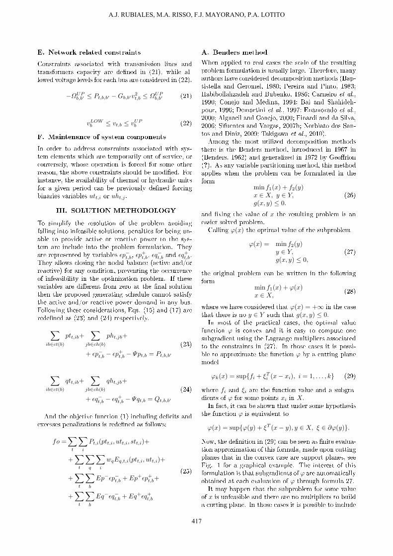
Now, the denition in (29) can be seen as nite evalua-tion approximation of this formula, made upon cuttingplanes that in the convex case are support planes, seeFig. 1 for a graphical example. The interest of thisformulation is that subgradients of ϕ are automaticallyobtained at each evaluation of ϕ through formula 27.It may happen that the subproblem for some value

of x is unfeasible and there are no multipliers to builda cutting plane. In those cases it is possible to include

A.J. RUBIALES, M.A. RISSO, F.J. MAYORANO, P.A. LOTITO

417

( )x

1( )x

2( )x3( )x

1x

2x 3x

Figure 1: Evolution of the cutting plane algorithm.

feasibility cuts, as it is shown in (Bonnans et al. ,2006), however, we will not need these cuts because inour case the subproblem is always feasible.The Benders method starts with an initial solution

x0 ∈ X and obtains the actual value ϕ(x0) solvingthe subproblem (27). After computing the rst k − 1iterations there is a point xk−1 and a cutting plane ap-proximation ϕk−1. Then it solves the master problem

min f1(x) + ϕk−1(x)x ∈ X, (30)

that, considering the formula (29), can be reformulatedas

min f1(x) + zx ∈ X,z ≥ fi + ξTi (x− xi), i = 1, . . . , k.

(31)

Calling xk the solution to the master problem, the al-gorithm keeps iterating until the gap between upperand lower bounds is small enough. The lower boundis given by the solution of the master problem and theupper bound is given by the solution to the subprob-lem.

B. Decomposed problem

The optimization problem of minimizing the function(1) constrained to (4-22) is written under the followingform

minym

fm(ym) + ϕ(ym), (32)

where ym represents the variable of the master prob-lem. The function ϕ is the objective function of thesubproblem, the variable of the subproblem is calledysp and fsp(ym, ysp) is the objective function of thesubproblem. Now, the constraints must be includedin each one of the problems. Dierent choices willcorrespond to a dierent behavior of the Benders al-gorithm. In this case all the binary variables and theactive power variables are considered for the masterproblem letting all the others variables belong to thesubproblem. We have then

ym = (utt,i, ptt,i, uht,j , pht,j , stt,i, ett,i) . (33)

For the master-problem objective function, we consid-ered the start-up costs of the thermal units toghetherwith the quadratic terms of the thermal generationcosts. Thus, we obtain

fm(ym) =∑t

∑i

Pt,i(ptt,i, utt,i, stt,i)+

+∑t

∑q

∑i

wqEq,t,i(ptt,i, utt,i)(34)

The constraints considered for the master problemsare all those that not contain the variables of the sub-problem: (4), (6-11), (13), (14), (19), (20).

Now the subproblem objective function becomes

fsp =∑t

∑b

Ep−εp−t,b + Ep+εp+t,b+

+ Eq−εq−t,b + Eq+εq+t,b.

(35)

Toghether with the variables that appear in this func-tion, the subproblem has also the reactive powervariables qtt,i, qht,j the corresponding slack variables(εp−t,b, εp

+t,b, εq

−t,b, εq

+t,b), the angles θt,b and the voltages

vt,b. The remaining constraints (5), (12), (15), (17),(21), (22) are considered in the subproblem with thevalues of master variables xed by the master problem.

With the proposed decomposition the resulting mas-ter problem is numerically more complex than the sub-problem. Indeed, it is a quadractic mixed integer prob-lem. The subproblem has a linear objective functionand non linear constrains, but the non linearity of theconstraints is non harmful in practice and the solversused can deal well with them.

It is worth mentioning also that the subproblem be-comes temporally uncoupled obtaining several optimalow problems where the values of the start-up vari-ables utt,i, uht,j and the active power generation ptt,i,pht,j are given by the master problem solution at eachiteration.

In order to simplify the introduction of cutting planeequations some dummy equations were added:

ptt,i = ptkt,i : µkt,i,

pht,j = phkt,j : λkt,j ,utt,i = utkt,i : πk

t,i,uht,j = uhkt,j : ψk

t,j ,

(36)

where uht,j , pht,j , utt,i y ptt,i are now subproblemvariables, uhkt,j , ph

kt,j , ut

kt,i y ptkt,i are given by the

master problem at the k iteration and µkt,i, λ

kt,j , ψ

kt,j ,

πkt,i are the corresponding multipliers.

The addition of cutting planes to the master prob-lem is made in the same way that in (30) and (31). Themaster objective function has the term

∑t zt which

corresponds with ϕ(ykm), and the cutting planes are:

Latin American Applied Research 42:413-425 (2012)

418

zt ≥ ztk +∑j

λkt,j(uht,j − uhkt,j)+

+∑j

ψkt,j(pht,j − phkt,j)+

+∑i

µkt,i(ptt,i − ptkt,i)+

+∑i

πkt,i(utt,i − utkt,i).

(37)

IV. RESULTS

In this section the main results obtained by apply-ing the proposed approach are presented. The appli-cation of the previously detailed algorithm are per-formed on systems of dierent sizes. Initially, a c-tional nine buses system presented in (Sifuentes andVargas, 2007a) is considered. Result details which aredicult to observe in larger systems can be consideredin this small example. Additionally, an application ofthe proposed methodology to a larger real power sys-tem is presented. One of the features which should beobserved in this section is the ability of the algorithmto consider the reactive power ow and see how thisfact impacts in the result. This is an important featureappreciated by system operators because no post dis-patch correction should be necessary. Voltage valuesat each bus are compared with results obtained fromPowerWorld Simulator (Overbye et al., 1995; Over-bye and Weber, 2000), which is a standard within theelectrical industry. Because this commercial softwaredoes not have the ability of solving the hydrothermalcoordination problem, power levels for each unit arexed with algorithm results, and voltage levels in eachbus are compared with PowerWorld Simulator valuesverifying its correctness.For the sake of clarity, all the technical details of the

example networks are given after the bibliography.

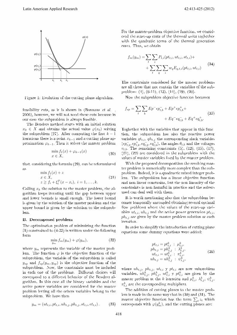
A. Nine buses test case

This system is based on a transmission network of 9buses with 9 lines. The generating equipment consistsof three thermal units and an hydroelectric one. Theobjectives of the tests performed on this system are:

• Analyze the impact of considering environmentalconstraints.

• Compare bus voltage values with PowerWorldSimulator results.

• Analyze algorithm convergence issues.

In Fig. 2 an one-line diagram of the 9-bus powersystem is presented. The Table 1, placed after thebibliography, details parameters like resistance (R), re-actance (X) and capacity.Costs, minimum and maximum power generation,

maximum active power dierence for two consecutive

Figure 2: 9-bus system one-line diagram.

Table 1: Power lines CharacteristicsFrom To R [Ohm] X [Ohm] Capacity [MW]N1 N4 0.04287 0.23341 250N3 N6 0.00471 0.02944 250N4 N5 0.03862 0.25562 250N4 N9 0.04689 0.31566 250N6 N5 0.04689 0.31566 300N6 N7 0.10193 0.59263 250N8 N7 0.04396 0.36805 150N8 N2 0.00476 0.02944 150N9 N8 0.04534 0.36943 250

periods and environmental coecients for each unitare described in Tables 2, 3 and 4.

Table 2: Thermal units power parametersName Active Power Reactive Power

Min Max ∆PTUP Min MaxT1 10 250 50 -100 100T2 10 300 50 -100 100T3 10 270 50 -100 100

Hydrothermal unit (H1) and its reservoir character-istics are enumerated in table 5 and 6 respectively. Forthe sake of simplicity, the relation between power gen-erated and water ow rate is modeled by a linear factorβj = 3.846 MW/m3/s.Table 7 describes the system demand and Spinning

Reserve (ζt ) during the whole day. It should be men-tioned that the spinning reserve is calculated as 15%of the total demand in each period.Penalty coecient Ep−, Ep+, Eq− and Eq+ are de-

ned as 1e6 for this example. It should be mentionedthat because in this example there are not fuel con-sumption constraints, Eq. (10) is not considered.

A.1. Convergence Analysis

In this section a brief analysis of the algorithm con-vergence considering and without considering environ-mental constraints is done. In Fig. 3 convergence of

A.J. RUBIALES, M.A. RISSO, F.J. MAYORANO, P.A. LOTITO

419

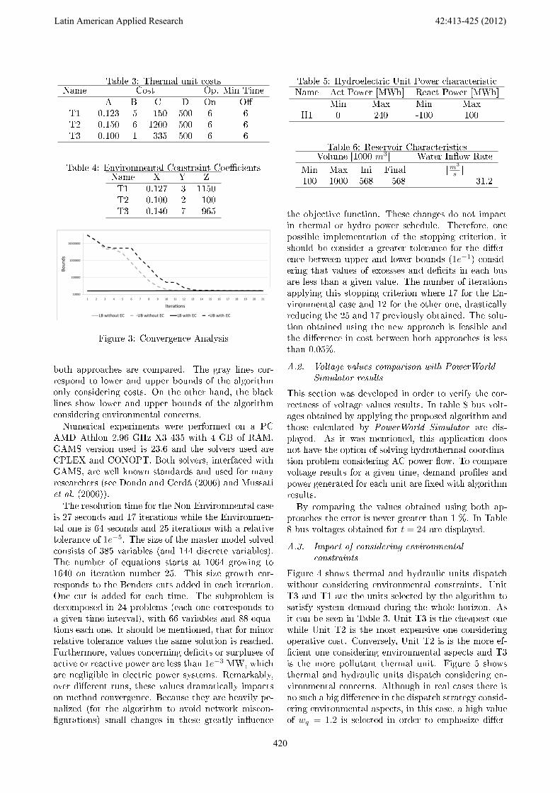
Table 3: Thermal unit costsName Cost Op. Min Time

A B C D On OT1 0.123 5 150 500 6 6T2 0.150 6 1200 500 6 6T3 0.100 1 335 500 6 6

Table 4: Environmental Constraint CoecientsName X Y ZT1 0.127 3 1150T2 0.100 2 100T3 0.140 7 965

100000

1000000

10000000

Boun

ds

10000

1 2 3 4 5 6 7 8 9 10 11 12 13 14 15 16 17 18 19 20 21

Iterations

LB without EC UB without EC LB with EC UB with EC

Figure 3: Convergence Analysis

both approaches are compared. The gray lines cor-respond to lower and upper bounds of the algorithmonly considering costs. On the other hand, the blacklines show lower and upper bounds of the algorithmconsidering environmental concerns.

Numerical experiments were performed on a PCAMD Athlon 2.96 GHz X3 435 with 4 GB of RAM.GAMS version used is 23.6 and the solvers used areCPLEX and CONOPT. Both solvers, interfaced withGAMS, are well known standards and used for manyresearchers (see Dondo and Cerdá (2006) and Mussatiet al. (2006)).

The resolution time for the Non-Environmental caseis 27 seconds and 17 iterations while the Environmen-tal one is 64 seconds and 25 iterations with a relativetolerance of 1e−5. The size of the master model solvedconsists of 385 variables (and 144 discrete variables).The number of equations starts at 1064 growing to1640 on iteration number 25. This size growth cor-responds to the Benders cuts added in each iteration.One cut is added for each time. The subproblem isdecomposed in 24 problems (each one corresponds toa given time interval), with 66 variables and 88 equa-tions each one. It should be mentioned, that for minorrelative tolerance values the same solution is reached.Furthermore, values concerning decits or surpluses ofactive or reactive power are less than 1e−3 MW, whichare negligible in electric power systems. Remarkably,over dierent runs, these values dramatically impactson method convergence. Because they are heavily pe-nalized (for the algorithm to avoid network miscon-gurations) small changes in these greatly inuence

Table 5: Hydroelectric Unit Power characteristicName Act Power [MWh] React Power [MWh]

Min Max Min MaxH1 0 240 -100 100

Table 6: Reservoir CharacteristicsVolume [1000 m3] Water Inow Rate

Min Max Ini Final [m3

s ]100 1000 568 568 31.2

the objective function. These changes do not impactin thermal or hydro power schedule. Therefore, onepossible implementation of the stopping criterion, itshould be consider a greater tolerance for the dier-ence between upper and lower bounds (1e−1) consid-ering that values of excesses and decits in each busare less than a given value. The number of iterationsapplying this stopping criterion where 17 for the En-vironmental case and 12 for the other one, drasticallyreducing the 25 and 17 previously obtained. The solu-tion obtained using the new approach is feasible andthe dierence in cost between both approaches is lessthan 0.05%.

A.2. Voltage values comparison with PowerWorldSimulator results

This section was developed in order to verify the cor-rectness of voltage values results. In table 8 bus volt-ages obtained by applying the proposed algorithm andthose calculated by PowerWorld Simulator are dis-played. As it was mentioned, this application doesnot have the option of solving hydrothermal coordina-tion problem considering AC power ow. To comparevoltage results for a given time, demand proles andpower generated for each unit are xed with algorithmresults.

By comparing the values obtained using both ap-proaches the error is never greater than 1 %. In Table8 bus voltages obtained for t = 24 are displayed.

A.3. Impact of considering environmentalconstraints

Figure 4 shows thermal and hydraulic units dispatchwithout considering environmental constraints. UnitT3 and T1 are the units selected by the algorithm tosatisfy system demand during the whole horizon. Asit can be seen in Table 3, Unit T3 is the cheapest onewhile Unit T2 is the most expensive one consideringoperative cost. Conversely, Unit T2 is is the more ef-cient one considering environmental aspects and T3is the more pollutant thermal unit. Figure 5 showsthermal and hydraulic units dispatch considering en-vironmental concerns. Although in real cases there isno such a big dierence in the dispatch strategy consid-ering environmental aspects, in this case, a high valueof wq = 1.2 is selected in order to emphasize dier-

Latin American Applied Research 42:413-425 (2012)

420

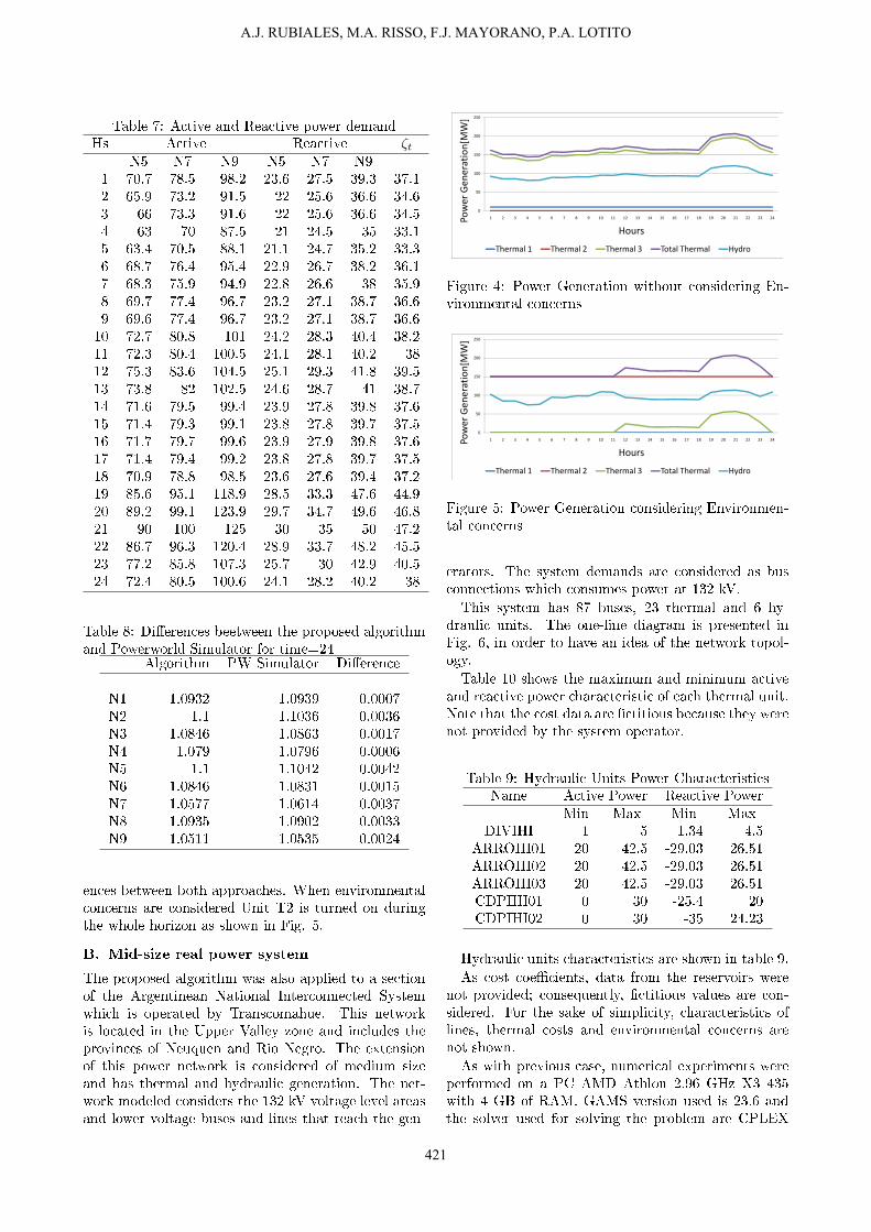
Table 7: Active and Reactive power demandHs Active Reactive ζt

N5 N7 N9 N5 N7 N91 70.7 78.5 98.2 23.6 27.5 39.3 37.12 65.9 73.2 91.5 22 25.6 36.6 34.63 66 73.3 91.6 22 25.6 36.6 34.54 63 70 87.5 21 24.5 35 33.15 63.4 70.5 88.1 21.1 24.7 35.2 33.36 68.7 76.4 95.4 22.9 26.7 38.2 36.17 68.3 75.9 94.9 22.8 26.6 38 35.98 69.7 77.4 96.7 23.2 27.1 38.7 36.69 69.6 77.4 96.7 23.2 27.1 38.7 36.610 72.7 80.8 101 24.2 28.3 40.4 38.211 72.3 80.4 100.5 24.1 28.1 40.2 3812 75.3 83.6 104.5 25.1 29.3 41.8 39.513 73.8 82 102.5 24.6 28.7 41 38.714 71.6 79.5 99.4 23.9 27.8 39.8 37.615 71.4 79.3 99.1 23.8 27.8 39.7 37.516 71.7 79.7 99.6 23.9 27.9 39.8 37.617 71.4 79.4 99.2 23.8 27.8 39.7 37.518 70.9 78.8 98.5 23.6 27.6 39.4 37.219 85.6 95.1 118.9 28.5 33.3 47.6 44.920 89.2 99.1 123.9 29.7 34.7 49.6 46.821 90 100 125 30 35 50 47.222 86.7 96.3 120.4 28.9 33.7 48.2 45.523 77.2 85.8 107.3 25.7 30 42.9 40.524 72.4 80.5 100.6 24.1 28.2 40.2 38

Table 8: Dierences beetween the proposed algorithmand Powerworld Simulator for time=24

Algorithm PW Simulator Dierence

N1 1.0932 1.0939 0.0007N2 1.1 1.1036 0.0036N3 1.0846 1.0863 0.0017N4 1.079 1.0796 0.0006N5 1.1 1.1042 0.0042N6 1.0846 1.0831 0.0015N7 1.0577 1.0614 0.0037N8 1.0935 1.0902 0.0033N9 1.0511 1.0535 0.0024

ences between both approaches. When environmentalconcerns are considered Unit T2 is turned on duringthe whole horizon as shown in Fig. 5.

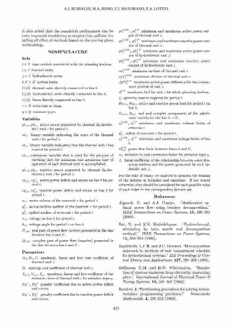
B. Mid-size real power system

The proposed algorithm was also applied to a sectionof the Argentinean National Interconnected Systemwhich is operated by Transcomahue. This networkis located in the Upper Valley zone and includes theprovinces of Neuquen and Rio Negro. The extensionof this power network is considered of medium sizeand has thermal and hydraulic generation. The net-work modeled considers the 132 kV voltage level areasand lower voltage buses and lines that reach the gen-

50

100

150

200

250

er Generation[M

W]

0

1 2 3 4 5 6 7 8 9 10 11 12 13 14 15 16 17 18 19 20 21 22 23 24Powe

Hours

Thermal 1 Thermal 2 Thermal 3 Total Thermal Hydro

Figure 4: Power Generation without considering En-vironmental concerns

50

100

150

200

250

er Generation[M

W]

0

1 2 3 4 5 6 7 8 9 10 11 12 13 14 15 16 17 18 19 20 21 22 23 24Powe

Hours

Thermal 1 Thermal 2 Thermal 3 Total Thermal Hydro

Figure 5: Power Generation considering Environmen-tal concerns

erators. The system demands are considered as busconnections which consumes power at 132 kV.

This system has 87 buses, 23 thermal and 6 hy-draulic units. The one-line diagram is presented inFig. 6, in order to have an idea of the network topol-ogy.

Table 10 shows the maximum and minimum activeand reactive power characteristic of each thermal unit.Note that the cost data are ctitious because they werenot provided by the system operator.

Table 9: Hydraulic Units Power CharacteristicsName Active Power Reactive Power

Min Max Min MaxDIVIHI 1 5 -1.34 4.5

ARROHI01 20 42.5 -29.03 26.51ARROHI02 20 42.5 -29.03 26.51ARROHI03 20 42.5 -29.03 26.51CDPIHI01 0 30 -25.4 20CDPIHI02 0 30 -35 24.23

Hydraulic units characteristics are shown in table 9.

As cost coecients, data from the reservoirs werenot provided; consequently, ctitious values are con-sidered. For the sake of simplicity, characteristics oflines, thermal costs and environmental concerns arenot shown.

As with previous case, numerical experiments wereperformed on a PC AMD Athlon 2.96 GHz X3 435with 4 GB of RAM. GAMS version used is 23.6 andthe solver used for solving the problem are CPLEX

A.J. RUBIALES, M.A. RISSO, F.J. MAYORANO, P.A. LOTITO

421

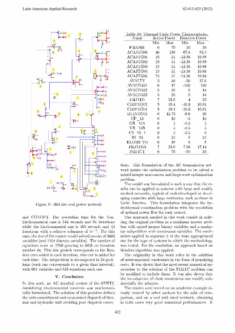
Figure 6: Mid-size real power network

and CONOPT. The resolution time for the Non-Environmental case is 544 seconds and 51 iterationswhile the Environmental one is 465 seconds and 44iterations with a relative tolerance of 1e−3. For thiscase, the size of the master model solved consist of 2665variables (and 1104 discrete variables). The number ofequations start at 7789 growing to 8821 on iterationnumber 44. This size growth corresponds to the Ben-ders cuts added in each iteration. One cut is added foreach time. The subproblem is decomposed in 24 prob-lems (each one corresponds to a given time interval),with 601 variables and 815 equations each one.

V. Conclusion

In this work, an AC detailed version of the STHTCconsidering environmental concerns was mathemati-cally formulated. The solution of this problem denesthe unit-commitment and economical dispatch of ther-mal and hydraulic unit avoiding post-dispatch correc-

Table 10: Thermal Units Power CharacteristicsName Active Power Reactive Power

Min Max Min MaxP.BAND. 0 70 -50 50ACAJTG06 40 130 -67.5 82.5ACAJTG01 15 51 -13.38 19.88ACAJTG02 15 51 -13.38 19.88ACAJTG03 15 51 -13.38 19.88ACAJTG04 15 51 -13.38 19.88ACAJTG05 15 51 -13.38 19.88AVALTV 3 30 -30 37.6AVALTG21 0 17 -100 100AVALTG22 5 26 0 14AVALTG23 5 26 0 14FILOTG 7 23.6 -4 23

CHIUTG02 5 19.4 -10.3 10.81CHIUTG01 5 19.4 -10.3 10.81HUINTG01 0 42.73 -8.6 30CP_13 0 10 -5 10GR_13A 0 5 -2.5 5VR_13B 0 5 -2.5 5CS_13_1 0 5 -2.5 0RI_33 0 25 0 25

ELOM2 TG 0 18 -5 8FILOTG3 7 23.6 -7.05 17.14PHFICT 0 70 -50 50

tions. This formulation of the AC transmission net-work makes the optimization problem to be solved amixed-integer non-convex and large scale optimizationproblem.The model was formulated in such a way that the re-

sults can be applied to systems with large and weaklymeshed networks, typical of underdeveloped or devel-oping countries with large territories, such as those inLatin America. This formulation integrates the hy-drothermal coordination problem with the resolutionof optimal power ow for each period.The approach applied in this work consist in split-

ting the original problem in a nonlinear master prob-lem with mixed integer binary variables and a nonlin-ear subproblem with continuous variables. The mech-anism applied to separate it is the most appropriatedone for the type of systems in which the methodologywas tested. For the resolution, an approach based onBenders algorithm was applied.The originality in this work relies in the addition

of environmental constraints in the form of penalizingcosts. It was shown that the most recent numerical ap-proaches to the solution of the STHTC problem canbe modied to include them. It was also shown thatthe introduction of these constraints can modify sub-stantially the solution.The results were tested on an academic example al-

ready treated by other authors for the sake of com-parison, and on a real mid sized network, obtainingin both cases very good numerical performances. It

Latin American Applied Research 42:413-425 (2012)

422

is also noted that the numerical performance can beeven improved considering strategies that palliate thetailing o eect of methods based on the cutting planemethodology.

NOMENCLATURE

Sets

t ∈ T time periods associated with the planning horizon.

i ∈ I thermal units.

j ∈ J hydroelectric units.

b, b′ ∈ B system buses.

Ct(b) thermal units directly connected to bus b.

Ch(b) hydroelectric units directly connected to bus b.

Cb(b) buses directly connected to bus b.

r ∈ R reservoirs or dams.

q ∈ Q emission types.

Variables

ptt,i, pht,i active power generated by thermal (hydroelec-tric) unit i for period t.

utt,i binary variable indicating the state of the thermalunit i for period t.

stt,i binary variable indicating that the thermal unit i hasstarted for period t.

ett,i continuous variable that is used for the purpose ofchecking that the minimum and maximum time ofoperation of each thermal unit is accomplished.

qtt,i, qht,i reactive power generated by thermal (hydro-electric) unit i for period t.

εp−t,b, εp+t,b active power decit and excess on bus b for pe-

riod t.

εq−t,b, εq+t,b reactive power decit and excess on bus b for

period t.

at,r water volume of the reservoir r for period t.

qTt,r across-turbine outow of the reservoir r for period t.

qSt,r spilled outow of reservoir r for period t.

vt,b voltage on bus b for period t.

θt,b voltage angle for period t on bus b.

Pt,bb′ real part of power ow (active) presented in the linebetween bus b and b′.

Qt,bb′ complex part of power ow (reactive) presented inthe line between bus b and b′.

Parameters

Ai, Bi, Ci quadratic, linear and free cost coecient ofthermal unit i.

Di start-up cost coecient of thermal unit i.

Xq,i, Yq,i, Zq,i quadratic, linear and free coecient of theemission curve of thermal unit i for emission type q.

Ep−, Ep+ penalty coecient due to active power decitand excess.

Eq−, Eq+ penalty coecient due to reactive power decitand excess.

ptLOWi , ptUP

i minimum and maximum active power out-put of thermal unit i.

qtLOWi , qtUP

i minimum and maximum reactive power out-put of thermal unit i.

phLOWj , phUP

j minimum and maximum active power out-put of hydroelectric unit j.

qhLOWj , qhUP

j minimum and maximum reactive poweroutput of hydroelectric unit j.

onLOWi minimum on-time of thermal unit i.

offLOWi minimum o-time of thermal unit i.

∆PTUPi maximum active power dierence for two consec-utive periods of unit i.

ϑUPi maximum fuel for unit i for whole planning horizon.

ζt spinning reserve required for period t.

Ψpt,b, Ψqt,b active and reactive power load for period t onbus b.

Gb,b′ , Bb,b′ real and complex components of the admit-tance matrix for the line b→ b′.

aLOWr , aUP

r minimum and maximum volume limits ofreservoir r.

qIt,r inow of reservoir r for period t.

vLOWb , vUP

b minimum and maximum voltage limits of busb.

ΩUPb,b′ power ow limit between buses b and b′.

wq emission to cost conversion factor for emission type q.

βj linear coecient of the relationship between water owacross turbine and the power generated by each hy-draulic unit j.

For the sake of clarity we omitted to mention the domain

of the indexes in formulas and equations. If not stated

otherwise, they should be considered for each possible value

of each index in the corresponding domain set.

References

Alguacil, N. and A.J. Conejo, Multiperiod op-timal power ow using benders decomposition,IEEE Transactions on Power Systems, 15, 196201(2000).

Bai, X. and S.M. Shahidehpour, Hydro-thermal,scheduling by tabu search and decompositionmethod, IEEE Transactions on Power Systems,11, 968974 (1996).

Baptistella, L.F.B. and J.C. Geromel, Decompositionapproach to problem of unit commitment schedulefor hydrothermal systems, IEE Proceedings D Con-trol Theory and Applications, 127, 250258 (1980).

Bellhouse, G.M. and H.W. Whittington, Simula-tion of gaseous emissions from electricity generatingplant, International Journal of Electrical Power &Energy Systems, 18, 501507 (1996).

Benders, J. Partitioning procedures for solving mixed-variables programming problems, NumerischeMathematik, 4, 238252 (1962).

A.J. RUBIALES, M.A. RISSO, F.J. MAYORANO, P.A. LOTITO

423

Bonnans, J.F., J.C. Gilbert, C. Lemaréchal and C.A.Sagastizábal, Numerical Optimization: Theoreticaland Practical Aspects, SpringerVerlag, Berlin, Ger-many (2006).

Carneiro, A.A.F.M., S. Soares and P.S. Bond, Alarge scale of an optimal deterministic hydrother-mal scheduling algorithm, IEEE Transactions onPower Systems, 5, 204211 (1990).

Catalão, J., S. Mariano, V. Mendes and L. Ferreira,Short-term scheduling of thermal units: emissionconstraints and trade-o curves, European Trans-actions on Electrical Power, 18, 114 (2008).

Chen, P. and H. Chang, Genetic aided scheduling ofhydraulically coupled plants in hydro-thermal coor-dination, IEEE Transactions on Power Systems,11, 975981 (1996).

Conejo, A. and J. Medina, Long-term hydro-thermalcoordination via hydro and thermal subsystem de-composition, Proc. th Mediterranean Electrotech-nical Conf., 921924 (1994).

Demartini, G., T.R. De Simone, G.P. Granelli, M.Montagna and K. Robo, Dual programming meth-ods for large-scale thermal generation scheduling,Proc. 20th Int Power Industry Computer Applica-tions. Conf. (1997).

Diniz, A.L. and M.E.P. Maceira, A four-dimensionalmodel of hydro generation for the short-term hy-drothermal dispatch problem considering head andspillage eects, IEEE Transactions on Power Sys-tems, 23, 12981308 (2008).

Diniz, A.L., T.N. Santos and M.E.P. Maceira, Shortterm security constrained hydrothermal schedulingconsidering transmission losses, Proc. IEEE/PESTransmission & Distribution Conf. and Exposition:Latin America TDC '06, 16 (2006). doi:10.1109/TDCLA.2006.311437.

Dondo, R. and J. Cerdá, An MILP framework fordynamic vehicle routing problems with time win-dows, Latin American applied research, 36, 255261 (2006).

Enamorado, J.C., A. Ramos and T. Gomez, Multi-area decentralized optimal hydro-thermal coordina-tion by the dantzig-wolfe decomposition method,Proc. IEEE Power Engineering Society SummerMeeting, 4, 20272032 (2000).

Farhat I. and El-Hawary M. Optimization methods ap-plied for solving the short-term hydrothermal coor-dination problem. Electric Power Systems Research,79(9):13081320, 2009.

Finardi, E., E. da Silva and C. Sagastizábal, Solv-ing the unit commitment problem of hydropowerplants via Lagrangian Relaxation and SequentialQuadratic Programming, Computational & appliedmathematics, 24, 317342 (2005).

Finardi, E.C. and E.L. da Silva, Solving the hy-dro unit commitment problem via dual decom-position and sequential quadratic programming,IEEE Transactions on Power Systems, 21, 835844(2006).

Georion, A., Generalized benders decomposition,Journal of optimization theory and applications, 10,237260 (1972).

Grainger, J. and W. Stevenson, Power system analy-sis, 152, McGraw-Hill New York (1994).

Habibollahzadeh, H. and J.A. Bubenko, Applicationof decomposition techniques to short-term opera-tion planning of hydrothermal power system, IEEEPower Eng. Rev., 6, 2829 (1986).

Hillier, F., G. Lieberman and G. Liberman, Introduc-tion to operations research. McGraw-Hill New York(1990).

Lemaréchal, C. and C. Sagastizábal, Variable metricbundle methods: from conceptual to implementableforms, Mathematical Programming, 76, 393410(1997).

Lu, B. and M. Shahidehpour, Unit commitment withexible generating units, IEEE Transactions onPower Systems, 20, 10221034 (2005).

Murillo-Sanchez, C. and R. Thomas, Thermal unitcommitment including optimal AC power ow con-straints, Proceedings of the Hawaii InternationalConference on System Sciences, IEEE Institute ofElectrical and Electronics, 31, 8188 (1998).

Mussati, S.F., P.A. Aguirre and N.J. Scenna, Ther-modynamic approach for optimal design of heatand power plants: Relationships between thermo-dynamic and economics solutions, Latin Americanapplied research, 36, 329335 (2006).

Norbiato dos Santos, T. and A.L. Diniz, A newmultiperiod stage denition for the multistage ben-ders decomposition approach applied to hydrother-mal scheduling, IEEE Transactions on Power Sys-tems, 24, 13831392 (2009).

Ongsakul, W. and N. Petcharaks, Transmission con-strained generation scheduling in a centralized elec-tricity market by improved Lagrangian relaxation,IEEE Power Engineering Society General Meeting,11561163 (2005).

Latin American Applied Research 42:413-425 (2012)

424

Orero, S. and M. Irving, A genetic algorithm mod-elling framework and solution technique for shortterm optimal hydrothermal scheduling, IEEETransactions on Power Systems, 13, 501518(1998).

Overbye, T., P. Sauer, C. Marzinzik and G. Gross, Auser-friendly simulation program for teaching powersystem operations, IEEE Transactions on PowerSystems, 10, 17251733 (1995).

Overbye, T. and J. Weber, Visualization of powersystem data, Proceedings of the 33rd AnnualHawaii International Conference on System Sci-ences (2000).

Pereira, M.V.F. and L.M.V.G. Pinto, Application ofdecomposition techniques to the mid - and short -term scheduling of hydrothermal systems, IEEETrans. Power App. Syst., 102, 36113618 (1983).

Ramanathan, R., Emission constrained economic dis-patch, IEEE Transactions on Power Systems, 9,19942000 (1994).

Rubiales, A., F. Mayorano and P. Lotito, Opti-mización aplicada a la coordinación hidrotérmica delmercado eléctrico argentino, Mecánica Computa-cional, 26, 19061920 (2007).

Sifuentes, W. and A. Vargas, Short-term hydrother-mal coordination considering an ac network model-ing, International Journal of Electrical Power &Energy Systems, 29, 488496 (2007a).

Sifuentes, W.S. and A. Vargas, Hydrothermalscheduling using benders decomposition: Accelerat-ing techniques, IEEE Transactions on Power Sys-tems, 22, 13511359 (2007b).

Sinha, N. and L. Lai, Meta heuristic search algorithmsfor short-term hydrothermal scheduling, Interna-tional Conference on Machine Learning and Cyber-netics, 40504056 (2006).

Takigawa, F.Y.K., E.C. Finardi and E.L. da Silva,A decomposition strategy to solve the short-termhydrothermal scheduling based on lagrangian relax-ation, Proc. IEEE/PES Transmission and Distri-bution Conf. and Exposition: Latin America (T&D-LA), 681688 (2010).

Troncoso, A., J. Riquelme, J. Aguilar-Ruiz and J.Riquelme Santos, Evolutionary techniques appliedto the optimal short-term scheduling of the electri-cal energy production, European Journal of Oper-ational Research, 185, 11141127 (2008).

Wang, S.J., S.M. Shahidehpour, D.S. Kirschen, S.Mokhtari and G.D. Irisarri, Short-term genera-tion scheduling with transmission and environmen-tal constraints using an augmented lagrangian re-

laxation, IEEE Transactions on Power Systems,10, 12941301 (1995).

Wood, A. and B. Wollenberg, Power generation, op-eration, and control, Wiley New York (1984).

Yu, B., X. Yuan and J. Wang, Short-term hydro-thermal scheduling using particle swarm optimiza-tion method, Energy Conversion and Management,48, 19021908 (2007).

A.J. RUBIALES, M.A. RISSO, F.J. MAYORANO, P.A. LOTITO

425