SE

Ga

b

ARRAA

JCG

KOSD

1

asia1sbsl

aVi

0

Journal of Economic Behavior & Organization 101 (2014) 113–127

Contents lists available at ScienceDirect

Journal of Economic Behavior & Organization

j ourna l h om epa ge: w ww.elsev ier .com/ locate / jebo

hort sale constraints, divergence of opinion and asset prices:vidence from the laboratory�

erlinde Fellnera, Erik Theissenb,∗

Institute of Economics, Ulm University, Helmholtzstr. 18, 89081 Ulm, GermanyFinance Area, University of Mannheim, and Centre for Financial Research, Cologne, Germany

a r t i c l e i n f o

rticle history:eceived 25 November 2011eceived in revised form 6 February 2014ccepted 13 February 2014vailable online 26 February 2014

EL classification:9214

eywords:vervaluation hypothesishort selling constraintsivergence of opinion

a b s t r a c t

The overvaluation hypothesis (Miller, 1977) predicts that (a) stocks are overvalued in thepresence of short selling restrictions and that (b) the overvaluation increases in the degreeof divergence of opinion. We design an experiment that allows us to test these predictionsin the laboratory. The results indicate that prices are higher with short selling constraints,but the overvaluation does not increase in the degree of divergence of opinion. We furtherfind that trading volume is lower and quoted bid-ask spreads tend to be higher when shortsale restrictions are imposed.

© 2014 Elsevier B.V. All rights reserved.

. Introduction

The implications of short sale restrictions on asset prices and market quality have received an unprecedented level ofttention by both academics and practitioners in the wake of the 2008 short sale ban. The fundamental question is whetherhort sale restrictions result in overvaluation, as suggested by Miller (1977). Although the overvaluation hypothesis isncompatible with a rational expectations equilibrium (Diamond and Verrecchia, 1987), it has received much attention (and

fair amount of empirical support) in the literature. The first wave of empirical studies dates from the 1980s and early990s; however, interest in the issue has been reignited in the 2000s, partially motivated by the question of whether shortelling constraints contributed to the internet bubble of the late nineties. A third, and still ongoing, wave of research has

een motivated by the short selling ban on financial stocks imposed by the SEC in September 2008. The imposition of thehort sale ban is a natural experiment which allows researchers to analyze the implications of short sale restrictions foriquidity and volatility, issues hardly addressed in the older empirical literature.

� We thank two anonymous referees, Brian Kluger, Stefan Nagel, participants of the 33rd annual meeting of the European Finance Association, the 14thnnual meeting of the German Finance Association, the meeting of SFB/TR15 in Caputh and seminar participants at the universities of Mannheim andienna for valuable comments. We are indebted to Rouhollah Mohammadi for his research assistance and to the BonnEconLab team (and Holger Gerhardt

n particular) for their hospitality and support. We gratefully acknowledge financial support from Deutsche Forschungsgemeinschaft through SFB/TR 15.∗ Corresponding author at: Finance Area, University of Mannheim, L 9 1-2, 68161 Mannheim, Germany. Tel.: +49 621 1811517; fax: +49 621 1811519.

E-mail addresses: gerlinde.fellner@uni-ulm.de (G. Fellner), theissen@uni-mannheim.de (E. Theissen).

http://dx.doi.org/10.1016/j.jebo.2014.02.010167-2681/© 2014 Elsevier B.V. All rights reserved.

114 G. Fellner, E. Theissen / Journal of Economic Behavior & Organization 101 (2014) 113–127

Our paper contributes to this literature by providing the first test of the overvaluation hypothesis in a controlled laboratorysetting.1 We argue that an experimental test is a valuable complement to empirical tests with field data because the latterare complicated by a number of impediments. Most importantly, neither the value of a stock nor the degree of divergenceof opinion (an important determinant of asset prices according to the overvaluation hypothesis) is directly observable.Consequently, researchers have to rely on proxies which may be noisy or even biased, and which may be correlated withother stock characteristics that affect valuation. It is thus not surprising that empirical tests of the overvaluation hypothesis,summarized briefly in Section 2, yield inconclusive results.

None of the measurement problems alluded to above is present in the laboratory. The experimenter controls the infor-mation structure and, consequently, the degree of divergence of opinion. Similarly, short sale constraints are imposed bythe experimenter. As identical assets can be traded with and without constraints, it is feasible to directly compare the mar-ket values of the assets, rather than inferring overvaluation from proxy variables or subsequent returns. The results of ourexperiments provide only partial support for the overvaluation hypothesis. Prices in the experimental markets are higherwhen short selling is prohibited. However, the overvaluation does not depend on the degree of divergence of opinion. Wefurther find that trading volume is lower and quoted bid-ask spreads are higher when short sale constraints are imposed.This is consistent with recent empirical evidence from the 2008 short selling ban.2

2. Literature

As noted in the introduction, the overvaluation hypothesis was first put forward by Miller (1977). The basic intuitionis simple: if traders have different opinions about the value of an asset, the optimists will buy and the pessimists will sell.However, short sale constraints prevent those pessimists not currently owning the asset from selling it. Optimistic opinionswill then be overrepresented in market prices. Consequently, short sale restrictions lead to overvaluation that increases inthe degree of divergence of opinion.

The overvaluation hypothesis is inconsistent with a rational expectations equilibrium.3 Diamond and Verrecchia (1987)present a rational expectations model in which short sale constraints do not lead to overvaluation but reduce the speed atwhich new information, negative information in particular, is incorporated into prices. Hong and Stein (2003) derive similarresults, though in a very different context. Recent theoretical research has revived the overvaluation hypothesis. Duffie et al.(2002) derive a model in which short sale constraints together with divergence of opinion (modeled by assuming differentpriors about the payoff distribution) may lead to overvaluation. In the model by Johnson (2004), higher degrees of divergenceof opinion lead to lower subsequent returns in a fully rational context. In Scheinkman and Xiong (2003), overconfidencecreates divergence of opinion and, in the presence of short sale constraints, may lead to overvaluation. A similar result isderived in Jiang (2005). Gallmeyer and Hollifield (2008) present a model in which the imposition of short sale constraintscan either increase or decrease stock prices, depending on the optimistic investors’ intertemporal elasticity of substitution.

Researchers have used various approaches in order to empirically test the overvaluation hypothesis. The most commonone is to consider a cross-section of stocks and to test whether stocks that are subject to short selling constraints areovervalued, and whether overvaluation depends on the degree of divergence of opinion. This requires (a) the identificationof stocks that are short sale constrained, (b) a measure of asset value to identify overvaluation and (c) a measure for thedegree of divergence of opinion.4

Various measures have been employed to identify short sale constrained stocks. These include considering theshort interest (Figlewski and Webb, 1993; Asquith and Meulbroek, 1995; Dechow et al., 2001; Desai et al., 2002;Asquith et al., 2005; Boehme et al., 2006; Cohen et al. 2007), institutional ownership (Asquith et al., 2005; Nagel, 2005;Berkman et al., 2009), the availability of options on the stock (Figlewski and Webb, 1993; Danielsen and Sorescu, 2001; May-hew and Mihov, 2004; Boehme et al., 2006; Phillips, 2011), the inclusion of a stock in the “threshold list” (Diether et al., 2005),the rebate rate (Jones and Lamont, 2002; Reed, 2007; Ofek et al., 2004; Boehme et al., 2006; Cohen et al. 2007) and failuresto deliver (Autore et al., 2011b; Diether and Werner, 2009). However, recent evidence on the amount of short selling (12.9%of NYSE volume in the period 2000–2004 as reported in Boehmer et al., 2008; 24% of NYSE volume and even 31% of Nasdaqvolume in 2005 as documented by Diether et al., 2009a) suggests that short selling constraints are not very widespread inthe U.S. stock market.

Some researchers identify overvalued stocks by analyzing valuation ratios (Dechow et al., 2001; Desai et al., 2002; Jones

and Lamont, 2002), by considering adjustments to analysts’ earnings forecasts (Francis et al., 2005) or by considering firmage or earnings volatility (Berkman et al., 2009). The most widespread approach is to rely on subsequent returns to identifyovervalued stocks. This approach is based on the implicit assumption that either short sale constraints are removed or the

1 We are aware of five other papers that vary the level of short selling constraints in the laboratory (King et al., 1993; Ackert et al., 2002; Haruvy andNoussair, 2006; Bhojraj et al., 2009; Hauser and Huber, 2012). As laid out in more detail in the following section, the designs of these experiments differfrom ours in a number of important ways.

2 See Beber and Pagano (2013), Boehmer et al. (2013), Boulton and Braga-Alves (2010), Fotak et al. (2009), Helmes et al. (2011).3 It is fair to note that Miller (1977) was well aware of the limitations of his model. He explicitly refers to the winner’s curse problem and argues (p.

1158) that “many investors are still following naive procedures”.4 Some papers use alternative approaches to test Miller’s hypothesis. Dong and Michel (2008) find that IPO undervaluation is increasing in measures of

the heterogeneity of investor beliefs. Greenwood (2009) reports that trading restrictions around stock splits in Japan result in overvaluation.

dN

ea

dDo

toDe(tttaab

(sltapccboiavettta2Bosbph

aes

fas

d

s

G. Fellner, E. Theissen / Journal of Economic Behavior & Organization 101 (2014) 113–127 115

ivergence of opinion is reduced (e.g., because new information is released), leading to a decrease in the level of overvaluation.egative returns are thus taken as evidence of initial overvaluation.

The most widely used proxy for the degree of divergence of opinion is the standard deviation of analyst forecasts (Diethert al., 2002; Boehme et al., 2006; Berkman et al., 2009), but the standard deviation of returns and the turnover ratio havelso been employed (Berkman et al., 2009; Boehme et al., 2006).

In summary, none of the variables of interest can easily be measured. In addition, the two explanatory variables – theegree to which a stock is short sale constrained and the degree of divergence of opinion – may not be independent.’Avolio (2002) documents that a stock is more likely to be “on special” (i.e., to be expensive to sell short) when the degreef divergence of opinion is high.

Given the measurement problems and the different approaches implemented to resolve them, it is not surprisinghat the results in the empirical literature are not unanimous. A majority of papers find results that are supportivef the overvaluation hypotheses (e.g., Figlewski and Webb, 1993; Danielsen and Sorescu, 2001; Dechow et al., 2001;esai et al., 2002; Diether et al., 2002; Jones and Lamont, 2002; Gopalan, 2003; Ofek et al., 2004; Boehme et al., 2006; Cohent al. 2007; Nagel, 2005; Berkman et al., 2009; Aitken et al., 1998; Chang et al., 2007; Berkman and Koch, 2008). Aitken et al.1998) make use of the fact that in Australia, short sales are transparent. Using intraday event study methodology, they findhat prices almost instantaneously decrease after a short sale. Chang et al. (2007) use data from Hong Kong, where only stockshat are included on a short sale list can be shorted. The list is revised from time to time. Additions to and deletions fromhe list are associated with abnormal returns, the sign of which is consistent with the overvaluation hypothesis. Berkmannd Koch (2008) analyze trading activity prior to earnings announcements. They find that trading in the wake of earningsnnouncements is dominated by buyer-initiated trades and that there are price run-ups particularly for stocks characterizedy low institutional ownership (which are difficult to sell short) and high degrees of divergence of opinion.

Other papers support the overvaluation hypothesis only partially, e.g., when equally weighted portfolios are consideredAsquith et al., 2005). Diether et al. (2005) find that returns of small stocks are negative after a period of increased shortelling (which is consistent with the overvaluation hypothesis) but that returns after inclusion of small firms in the thresholdist are, if anything, negative. The latter result is inconsistent with the overvaluation hypothesis because inclusion in thehreshold list implies more binding short sale restrictions. Brent et al. (1990) report that returns are not smaller in the monthfter an increase in short interest, which is also inconsistent with the overvaluation hypothesis. Mayhew and Mihov (2004)resent evidence suggesting that the negative returns around option listings documented by others are not robust. Theyonclude by stating (p. 22) that “we now believe that there is no credible evidence from option markets that a marginalhange in the cost of short selling can have an impact on prices.” Boehmer et al. (2010) find that there is no asymmetryetween the speeds at which positive and negative information are impounded into prices.5 This is inconsistent with thevervaluation hypothesis and leads the authors to conclude that “[o]ur results . . . cast doubt on existing theories of thempact of short sale constraints.”Kaplan et al. (2013) conduct an interesting field experiment. They worked with a largesset manager who randomly withheld some of the stocks in his portfolio from the lending market. This created exogenousariation in short sale restrictions which, according to the overvaluation hypothesis, should affect prices. However, Kaplant al. (2013) do not find evidence of a significant impact on prices. In a recent paper, Diether et al. (2009b) analyze whetherhe suspension of the short sale price tests mandated by the SEC (regulation SHO) affected stock returns. Because the priceests deter short selling, the overvaluation hypothesis predicts negative returns. However, the evidence is inconsistent withhat prediction. In an analysis of the internet bubble Battalio and Schultz (2006) find no evidence that short sale constraintsffected the prices of Internet stocks. Finally, several papers test whether the short sale ban imposed by the SEC in September008 led to an increase in the prices of the stocks that were subjected to the ban, and Autore et al. (2011a), Boulton andraga-Alves (2010), Gagnon and Witmer (2010) and Harris et al. (2013) find supporting evidence for an increase. However,btaining clear results is difficult because the Troubled Assets Relief Program and other programs were announced on theame day. From an analysis of stocks that were later added to the ban list, Boehmer et al. (2013) conclude that “the shortingan did not provide an artificial boost in prices.” Based on an analysis of stocks from 30 countries, Beber and Pagano (2013,. 345) conclude that “. . . in contrast to the regulators’ hopes, the overall evidence indicates that at best short-selling bansave left stock prices unaffected.”

Conflicting findings are provided by Bris et al. (2007) and Charoenrook and Daouk (2009). Both compare stock return char-cteristics in countries with and without short sale restrictions. The papers conclude that allowing short sales increases thefficiency of price discovery. Charoenrook and Daouk (2009) find that when countries start to allow short selling, aggregatetock returns increase. This is clearly inconsistent with the overvaluation hypothesis.6

In summary, even though a number of empirical papers find results supportive of the overvaluation hypothesis, it appears

air to conclude that the issue is not yet settled. The measurement issues alluded to above suggest that an experimentalpproach is called for. We are aware of five papers that address the effect of short sale constraints on pricing in a laboratoryetting. Three of these papers (King et al., 1993; Ackert et al., 2002; Haruvy and Noussair, 2006) build on the experiments

5 Au et al. (2009) arrive at a similar conclusion. They find that idiosyncratic volatility (which affects both short and long positions) is a more importanteterrent to short selling than short sale costs.6 Charoenrook and Daouk (2009) attribute their result to increased liquidity, which, in turn, lowers expected returns and thus leads to an increase in

tock prices.

116 G. Fellner, E. Theissen / Journal of Economic Behavior & Organization 101 (2014) 113–127

of Smith et al. (1988). These authors found evidence of persistent and frequent price bubbles in experimental markets fora long-lived asset with short sale constraints in place. King et al. (1993), Ackert et al. (2002) and Haruvy and Noussair(2006) test whether lifting the short selling constraints reduces the frequency and/or the magnitude of the bubbles. Theresults were mixed. King et al. (1993) find that a relaxation of the short sale constraints does not have much impact on theoccurrence of bubbles. Ackert et al. (2002), on the other hand, find prices closer to the fundamental value of the asset whenthe short sale restrictions are relaxed. Haruvy and Noussair (2006) use a more differentiated experimental design and findthat removing short sale restrictions reduces prices, but does not necessarily make them more efficient. In fact, when shortsales are allowed, prices may be significantly below the fundamental value. A common feature of these experiments is thattraders receive symmetric information about the asset value. Thus, there is no divergence of opinion.7 Consequently, noneof these papers can be considered a test of Miller’s (1977) overvaluation hypothesis because it states that the divergence ofopinion is a necessary condition for overvaluation to occur.

Bhojraj et al. (2009) run a series of experiments in which they vary margin requirements. This is similar to varyingthe degree of short sale constraints. The fundamental value of the asset in their experiments is fixed and known to alltraders. Thus, there is again no uncertainty (and, consequently, no divergence of opinion) about fundamentals. The price is adeterministic function of the excess demand. A robot (the “sentiment trader”) buys assets in each period, thus putting upwardpressure on the prices. If there are no short selling constraints, the traders should drive down the price to the fundamentalvalue. If restrictions are in place, the equilibrium price may be above the fundamental value. The results indicate thatrelaxing margin requirements (and thereby short sale constraints) can even exacerbate overpricing, which is at odds withthe overvaluation hypothesis. The experiments of Bhojraj et al. (2009) are designed to address how margin requirementsand, in particular, the risk of margin calls affect pricing efficiency. Given that (a) there is no fundamental uncertainty and(b) the presence of the sentiment trader drives equilibrium prices above fundamentals when short selling constraints arebinding, their experiments are not (and from our reading, not intended to be) a direct test of the overvaluation hypothesis.

The only experimental paper we are aware of that directly refers to Miller’s overvaluation hypothesis is Hauser and Huber(2012). In their experiments traders trade two assets which are in equal supply. One is a large (high-capitalization) assetand the other is a small (low capitalization) asset. The values of the two assets always add up to 100. As a consequence,there is no aggregate uncertainty in the market. The authors find that large assets tend to be undervalued in the presence ofshort-sale constraints while small assets tend to be overvalued. This asymmetry may be a consequence of the design featurethat the values of the two assets always add up to 100.

3. Experimental design and procedures

Our experimental design differs in a number of important ways from former experiments. Most importantly, in all but oneprevious experiments, subjects have symmetric information. Obviously, the degree of divergence of opinion cannot be variedin a symmetric information setting. Another important difference is that the experiments in three of the previous studies8

feature a long-lived asset with a fundamental value that declines through the course of the experiment. Endowments arenot re-initialized. Consequently, a subject exhausting her short selling capacity in one period is unable to sell in the nextperiod. In contrast, our experiments consist of stationary replications of a one-period economy.

In our experiment, subjects are divided into groups of ten traders. We refer to one such group as one market. In total, weconduct 24 such markets in which a total of 240 different subjects participate.9 Participants are recruited among studentsat the University of Bonn using the online recruiting system ORSEE (Greiner, 2004). The procedure of the experiment is asfollows. First, subjects are presented with a set of instructions that explain the experiment. These instructions, of whichan English translation can be found in Appendix, are read aloud to all subjects. Subjects are then given time to re-readthe instructions and ask questions. Second, to allow subjects to get acquainted with the computerized trading system, theexperiment starts with three training periods that are excluded from the analysis. Finally, there are 20 trading periods. In10 of these periods, short selling is prohibited, and in ten periods, it is allowed. We thus choose a within-subjects design,i.e., each market of 10 traders experiences both the short selling condition and the no short selling condition. To control fororder effects, in half of the markets the short selling condition was implemented first (A-P condition), and in the other halfthe no short selling condition was implemented first (P-A condition).

Subjects receive a 20D show-up fee for participation. In addition, at the end of the experiment, two trading periods (one

period of the no short selling condition and one period of the short selling condition) are determined randomly for payout.The profit of these periods is converted into Euros at a rate of 20 ECU10 = 1D and added to (or subtracted from) the show-upfee. The average payoff is 20.36D with a standard deviation of 13.55. The average duration of an experiment is about 90 min.

7 There may be differences of opinion due to strategic uncertainty, i.e., uncertainty with respect to the behavior of other subjects. Strategic uncertaintyis, however, not under the control of the experimenter.

8 The exception is Bhojraj et al. (2009).9 To check the robustness of our results, we re-invited 40 participants to take part in the experiment for a second time (in the same treatment) and thus

conducted four additional markets, one in each of the treatments displayed in Table 2. We refer to the data from these markets with experienced subjectswhen we investigate learning effects (see footnote 21).

10 In the experiment, all prices are denoted in Experimental Currency Units (ECU).

3

Twtf

vw

c

3

tw

or

a�aspi

3

ctvc

Hooct

G. Fellner, E. Theissen / Journal of Economic Behavior & Organization 101 (2014) 113–127 117

.1. Asset value and private signals

Subjects in the experiments trade a risky asset against a numéraire (cash, denoted Experimental Currency Units, ECU).he value of the asset is a random variable denoted V . To keep things simple, the asset value can be high (H) or low (L)ith equal probabilities. The realization is determined randomly at the beginning of each period but is only revealed after

he end of the trading period. Draws in different periods are independent of each other. We refer to the realization as theundamental value of the asset.

At the beginning of the period, each subject receives a private signal s that provides information on the fundamentalalue of the asset. The signal is either h (indicating a high value) or l (indicating a low value). The signal has precision phere p is the probability that the signal is correct, i.e.,

p = Prob(h|H) = Prob(l|L) (1)

The signal is uninformative if p = 0.5, it is informative but noisy if 0.5 < p < 1 and it is perfectly accurate if p = 1. The signalan be used to calculate the conditional expectation of the asset value as

E(V |s = h) = pH + (1 − p)L = L + p(H − L)

E(V |s = l) = pL + (1 − p)H = H − p(H − L)(2)

.2. Divergence of opinion

We wish to test the hypothesis that the overvaluation implied by the existence of short sale constraints increases inhe degree of divergence of opinion among traders. We therefore vary the degree of divergence of opinion across (but notithin) markets.

Our measure for the degree of divergence of opinion is the cross-sectional variance of the conditional expected valuef the asset. If the asset value is high (H), on average a fraction p of the traders receives the signal h and a fraction (1 − p)eceives the signal l. The mean of the conditional expectations is then

E[E(V |s)|V = H

]= p[L + p(H − L)] + (1 − p)[H − p(H − L)] = H − 2p(1 − p)(H − L) (3)

The cross-sectional variance of the conditional expected value of the asset is

Var[E(V |s)|V = H] = p{[L + p(H − L)] − [H − 2p(1 − p)(H − L)]}2 + (1 − p){[H − p(H − L)] − [H − 2p(1 − p)(H − L)]}2

= p(1 − p)(4p2 − 4p + 1)(H − L)2 (4)

The case of a low asset value is entirely symmetric and yields

E[E(V |s)|V = L] = L + 2p(1 − p)(H − L)Var[E(V |s)|V = L] = p(1 − p)(4p2 − 4p + 1)(H − L)2 (5)

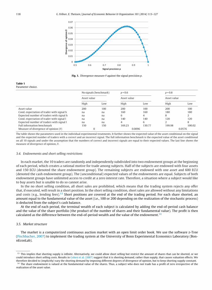
Thus, irrespective of the realization of the asset value,11 the cross-sectional variance of the conditional expectations of thesset value is proportional to � ≡ p(1 − p)(4p2 − 4p + 1). Therefore, we use � to measure the degree of divergence of opinion.

is zero when p = 0.5, because in this case, the signals are uninformative and the conditional expectations of the asset valuere equal to the unconditional expectation. � increases when the signal becomes informative. � approaches zero when theignal precision p goes to one. This is the case because the number of traders who receive a wrong signal goes to zero when

approaches 1. There exists a signal precision p that maximizes the degree of divergence of opinion. This maximum values obtained for p equal to 0.85. Fig. 1 graphs � as a function of p.

.3. Parameter choice

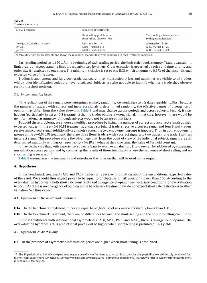
We choose the following parameters: H is set equal to 200, and L is set equal to 100. To vary divergence of opinion, wehoose two different signal precisions. In eight markets, p equals 0.6, and in other eight markets, p is equal to 0.8.12 The tworeatments are characterized by very different degrees of divergence of opinion. Table 1 shows the expectation of the assetalue conditional on the realization of the signal and its precision. It further presents the expected number of traders withorrect and incorrect signals and the measure � for the degree of divergence of opinion.

Previous experimental studies featuring a long-lived asset (e.g., Smith et al., 1988; King et al., 1993; Ackert et al., 2002;aruvy and Noussair, 2006) document that without a short selling possibility, overvaluation may arise even in the absencef asymmetric information. It is not clear whether this result extends to our design because we analyze static repetitionsf a one-period economy rather than a long-lived asset. Still, to test whether the same effect arises in our experiment, we

onduct eight markets with symmetric information. In these markets, subjects do not receive private signals. The results ofhese markets serve as a benchmark to measure the impact of divergence of opinion.

11 This is an implication of our assumption that the asset value is equally likely to be high or low.12 Including the markets with experienced subjects, 10 markets have a signal precision of p = 0.6 and 10 markets a signal precision of p = 0.8.

118 G. Fellner, E. Theissen / Journal of Economic Behavior & Organization 101 (2014) 113–127

0

0.01

0.02

0.03

0.04

0.05

0.06

0.07

0.5 0.6 0.7 0.8 0.9 1Di

verg

ence

of o

pini

onSignal precision p

Fig. 1. Divergence measure � against the signal precision p.

Table 1Parameter choice.

No signals (benchmark) p = 0.6 p = 0.8

Asset value Asset value Asset value

High Low High Low High Low

Asset value 200 100 200 100 200 100Cond. expectation of trader with signal h na na 160 160 180 180Expected number of traders with signal h na na 6 4 8 2Cond. expectation of trader with signal l na na 140 140 120 120Expected number of traders with signal l na na 4 6 2 8Full information benchmark 150 150 169.23 130.77 199.98 100.02Measure of divergence of opinion (�) 0 0.0096 0.0576

The table shows the parameters used in the individual experimental treatments. It further shows the expected value of the asset conditional on the signal

and the expected number of traders with a correct and an incorrect signal. The full information benchmark is the expected value of the asset conditionalon all 10 signals and under the assumption that the numbers of correct and incorrect signals are equal to their expected values. The last line shows themeasure of divergence of opinion, �.

3.4. Endowments and short selling restrictions

In each market, the 10 traders are randomly and independently subdivided into two endowment groups at the beginningof each period, which creates a rational motive for trade among subjects. Half of the subjects are endowed with four assetsand 150 ECU (denoted the share endowment group). The remaining subjects are endowed with one asset and 600 ECU(denoted the cash endowment group). The (unconditional) expected values of the endowments are equal. Subjects of bothendowment groups have unlimited access to credit at a zero interest rate. Therefore, a situation where a subject would liketo buy assets but is unable to do so cannot arise.

In the no short selling condition, all short sales are prohibited, which means that the trading system rejects any offerthat, if executed, will result in a short position. In the short selling condition, short sales are allowed without any limitationsand costs (e.g., lending fees).13 Short positions are covered at the end of the trading period. For each share shorted, anamount equal to the fundamental value of the asset (i.e., 100 or 200 depending on the realization of the stochastic process)is deducted from the subject’s cash balance.

At the end of each period, the terminal wealth of each subject is calculated by adding the end-of-period cash balanceand the value of the share portfolio (the product of the number of shares and their fundamental value). The profit is thencalculated as the difference between the end-of-period wealth and the value of the endowment.14

3.5. Market structure

The market is a computerized continuous auction market with an open limit order book. We use the software z-Tree

(Fischbacher, 2007) to implement the trading system at the University of Bonn Experimental Economics Laboratory (Bon-nEconLab).

13 This implies that shorting supply is infinite. Alternatively, we could allow short selling but restrict the amount of shares that can be shorted, or wecould introduce short selling costs. Results in Cohen et al. (2007) suggest that it is shorting demand, rather than supply, that causes valuation effects. Wetherefore decided to (implicitly) vary the shorting demand by imposing different degrees of divergence of opinion, but to keep shorting supply constant.

14 The share endowment is valued at the fundamental value of the shares. Thus, a subject who does not trade has a profit of zero irrespective of therealization of the asset value.

G. Fellner, E. Theissen / Journal of Economic Behavior & Organization 101 (2014) 113–127 119

Table 2Treatment summary.

Signal precision Sequence of treatments

Short selling prohibited –short selling allowed (PA)

Short selling allowed – shortselling prohibited (AP)

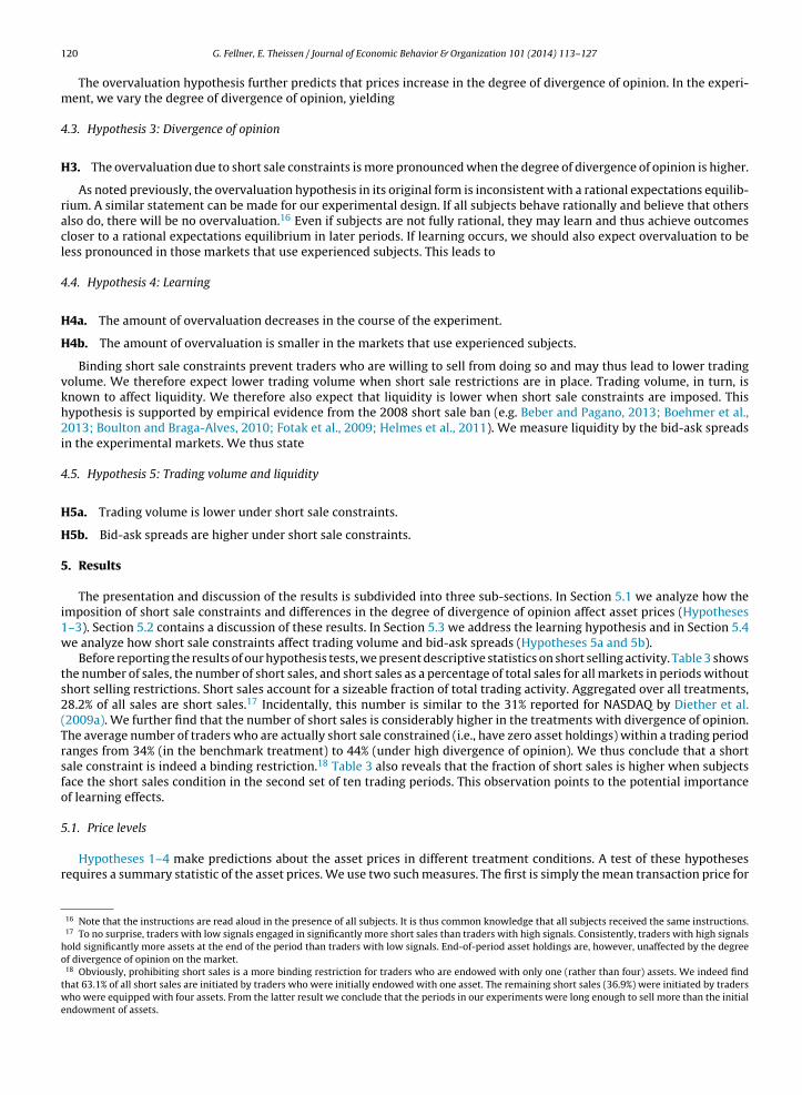
No signals (benchmark case) PA0 – market 1–4 AP0 market 13–16

T

loe

wr

3

tohn

ergid

ms

4

ootv

4

H

H

o

4

H

mi

p = 0.6 PA60 – market 5–8 AP60 market 17–20p = 0.8 PA80 – market 9–12 AP80 market 21–24

he table describes the treatments and shows the number of markets that were conducted in each treatment condition.

Each trading period lasts 150 s. At the beginning of each trading period, the limit order book is empty. Traders can submitimit orders or accept standing limit orders submitted by others. Order execution is governed by price and time priority andrder size is restricted to one share. The minimum tick size is set to one ECU which amounts to 0.67% of the unconditionalxpected value of the asset.

Trading is anonymous and fully post-trade transparent, i.e., transaction prices and quantities are visible to all tradershile trader identification codes are never displayed. Subjects are also not able to identify whether a trade they observe

esults in a short position.

.6. Implementation issues

If the realizations of the signals were determined entirely randomly, we would face two (related) problems. First, becausehe number of traders with correct and incorrect signals is determined randomly, the effective degree of divergence ofpinion may differ from the value shown in Table 1 and may change across periods and across cohorts. Second, it mayappen (particularly in the p = 0.8 treatment) that no trader obtains a wrong signal. In that case, however, there would beo informational asymmetry (although subjects would not be aware of that fact).

To avoid these problems, we choose a modified procedure by fixing the number of correct and incorrect signals at theirxpected values. In the p = 0.6 [0.8] treatments, always six [eight] traders receive a correct signal and four [two] traderseceive an incorrect signal. Additionally, symmetry across the two endowment groups is imposed. Thus, in both endowmentroups of the p = 0.6 [0.8] treatment, there are three [four] traders with a correct signal and two traders [one trader] with anncorrect signal. This procedure offers the advantage that, from the point of view of the individual subject, signals are stilletermined randomly with known precision p = 0.6 [0.8], while at the same time, the value of � is held constant.

It may be the case that, with experience, subjects learn to avoid overvaluation. This issue can be addressed by comparingisvaluation across periods and by comparing the results of those treatments where the sequence of short selling and no

hort selling is reversed.15

Table 2 summarizes the treatments and introduces the notation that will be used in the sequel.

. Hypotheses

In the benchmark treatment (AP0 and PA0), traders only receive information about the unconditional expected valuef the asset. We should thus expect prices to be equal to or (because of risk aversion) lower than 150. According to thevervaluation hypothesis, both short sale constraints and divergence of opinion are necessary conditions for overvaluationo occur. As there is no divergence of opinion in the benchmark treatment, we do not expect short sale restrictions to affectaluation. We thus expect

.1. Hypothesis 1: The benchmark treatment

1a. In the benchmark treatment, prices are equal to or (because of risk aversion) slightly lower than 150.

1b. In the benchmark treatment, there are no differences between the short-selling and the no short-selling conditions.

In those treatments with informational asymmetries (PA60, AP60, PA80 and AP80), there is divergence of opinion. Thevervaluation hypothesis thus predicts that prices will be higher when short selling is prohibited. This yields

.2. Hypothesis 2: Short selling

2. In the presence of asymmetric information, prices are higher when short selling is prohibited.

15 The 20 periods of an individual experiment may not be sufficient for learning to occur. To account for this possibility, we additionally conducted fourarkets with experienced subjects, i.e., subjects who have already participated in a previous experimental market. We refer to evidence from these markets

n Section 5.3, footnote 21.

120 G. Fellner, E. Theissen / Journal of Economic Behavior & Organization 101 (2014) 113–127

The overvaluation hypothesis further predicts that prices increase in the degree of divergence of opinion. In the experi-ment, we vary the degree of divergence of opinion, yielding

4.3. Hypothesis 3: Divergence of opinion

H3. The overvaluation due to short sale constraints is more pronounced when the degree of divergence of opinion is higher.

As noted previously, the overvaluation hypothesis in its original form is inconsistent with a rational expectations equilib-rium. A similar statement can be made for our experimental design. If all subjects behave rationally and believe that othersalso do, there will be no overvaluation.16 Even if subjects are not fully rational, they may learn and thus achieve outcomescloser to a rational expectations equilibrium in later periods. If learning occurs, we should also expect overvaluation to beless pronounced in those markets that use experienced subjects. This leads to

4.4. Hypothesis 4: Learning

H4a. The amount of overvaluation decreases in the course of the experiment.

H4b. The amount of overvaluation is smaller in the markets that use experienced subjects.

Binding short sale constraints prevent traders who are willing to sell from doing so and may thus lead to lower tradingvolume. We therefore expect lower trading volume when short sale restrictions are in place. Trading volume, in turn, isknown to affect liquidity. We therefore also expect that liquidity is lower when short sale constraints are imposed. Thishypothesis is supported by empirical evidence from the 2008 short sale ban (e.g. Beber and Pagano, 2013; Boehmer et al.,2013; Boulton and Braga-Alves, 2010; Fotak et al., 2009; Helmes et al., 2011). We measure liquidity by the bid-ask spreadsin the experimental markets. We thus state

4.5. Hypothesis 5: Trading volume and liquidity

H5a. Trading volume is lower under short sale constraints.

H5b. Bid-ask spreads are higher under short sale constraints.

5. Results

The presentation and discussion of the results is subdivided into three sub-sections. In Section 5.1 we analyze how theimposition of short sale constraints and differences in the degree of divergence of opinion affect asset prices (Hypotheses1–3). Section 5.2 contains a discussion of these results. In Section 5.3 we address the learning hypothesis and in Section 5.4we analyze how short sale constraints affect trading volume and bid-ask spreads (Hypotheses 5a and 5b).

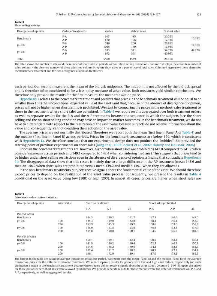
Before reporting the results of our hypothesis tests, we present descriptive statistics on short selling activity. Table 3 showsthe number of sales, the number of short sales, and short sales as a percentage of total sales for all markets in periods withoutshort selling restrictions. Short sales account for a sizeable fraction of total trading activity. Aggregated over all treatments,28.2% of all sales are short sales.17 Incidentally, this number is similar to the 31% reported for NASDAQ by Diether et al.(2009a). We further find that the number of short sales is considerably higher in the treatments with divergence of opinion.The average number of traders who are actually short sale constrained (i.e., have zero asset holdings) within a trading periodranges from 34% (in the benchmark treatment) to 44% (under high divergence of opinion). We thus conclude that a shortsale constraint is indeed a binding restriction.18 Table 3 also reveals that the fraction of short sales is higher when subjectsface the short sales condition in the second set of ten trading periods. This observation points to the potential importanceof learning effects.

5.1. Price levels

Hypotheses 1–4 make predictions about the asset prices in different treatment conditions. A test of these hypothesesrequires a summary statistic of the asset prices. We use two such measures. The first is simply the mean transaction price for

16 Note that the instructions are read aloud in the presence of all subjects. It is thus common knowledge that all subjects received the same instructions.17 To no surprise, traders with low signals engaged in significantly more short sales than traders with high signals. Consistently, traders with high signals

hold significantly more assets at the end of the period than traders with low signals. End-of-period asset holdings are, however, unaffected by the degreeof divergence of opinion on the market.

18 Obviously, prohibiting short sales is a more binding restriction for traders who are endowed with only one (rather than four) assets. We indeed findthat 63.1% of all short sales are initiated by traders who were initially endowed with one asset. The remaining short sales (36.9%) were initiated by traderswho were equipped with four assets. From the latter result we conclude that the periods in our experiments were long enough to sell more than the initialendowment of assets.

G. Fellner, E. Theissen / Journal of Economic Behavior & Organization 101 (2014) 113–127 121

Table 3Short selling activity.

Divergence of opinion Order of treatments #sales #short sales % short sales

BenchmarkP-A 913 185 20.26%

16.32%A-P 870 106 12.18%

p = 0.6P-A 746 200 26.81%

19.26%A-P 1066 149 13.98%

p = 0.8P-A 933 511 54.77% 47.72%A-P 972 398 40.95%

Total 5500 1549 28.16%

The table shows the number of sales and the number of short sales in periods without short selling restrictions. Column 3 displays the absolute number ofsales, column 4 the absolute number of short sales, and column 5 reports short sales as a percentage of total sales. Column 6 aggregates these shares fort

eat

sptashv

tws

cb1m

ec

TP

TtdfA

he benchmark treatment and the two divergence of opinion treatments.

ach period. Our second measure is the mean of the bid-ask midpoints. The midpoint is not affected by the bid-ask spreadnd is therefore often considered to be a less noisy measure of asset value. Both measures yield similar conclusions. Weherefore only present the results for the first measure, the mean transaction price.

Hypothesis 1 relates to the benchmark treatment and predicts that prices in the benchmark treatment will be equal to ormaller than 150 (the unconditional expected value of the asset) and that, because of the absence of divergence of opinion,rices will not be higher when short selling is prohibited. We start by comparing the prices in the no short-sales treatment tohose in the treatment where short sales are permitted. In Table 4 we report results aggregated over both treatment orderss well as separate results for the P-A and the A-P treatments because the sequence in which the subjects face the shortelling and the no short selling condition may have an impact on market outcomes. In the benchmark treatment, we do notave to differentiate with respect to the realization of the asset value because subjects do not receive information about thealue and, consequently, cannot condition their actions on the asset value.

The average prices are not normally distributed. Therefore we report both the mean (first line in Panel A of Table 4) andhe median (first line in Panel B) across periods. Prices for the benchmark treatments are below 150, which is consistentith Hypothesis 1a. We therefore conclude that our experimental design does not produce the “bubbles” that provided the

tarting point of previous experiments on short sales (King et al., 1993; Ackert et al., 2002; Haruvy and Noussair, 2006).Prices in the benchmark treatments are, however, higher when short sales are prohibited (147.0 compared to 141.7 when

onsidering means across periods and 149.1 compared to 142.4 when considering medians). This suggests that prices tend toe higher under short selling restrictions even in the absence of divergence of opinion, a finding that contradicts Hypothesisb. The disaggregated data show that this result is mainly due to a large difference in the AP treatment (mean 146.6 andedian 148.2 when short sales are prohibited versus mean 139.2 and median 139.1 when they are allowed).

In the non-benchmark treatments, subjects receive signals about the fundamental value of the asset. We should therefore

xpect prices to depend on the realization of the asset value process. Consequently, we present the results in Table 4onditional on the asset value being low (100) or high (200). In almost all cases, prices are higher when short sales are

able 4rice levels – descriptive statistics.

Divergence of opinion Asset value Short sales allowed Short sales prohibited

P-A A-P all P-A A-P all

Panel A: MeanBenchmark 144.3 139.2 141.7 147.3 146.6 147.0p = 0.6 100 145.3 139.0 142.0 158.3 146.1 152.0

200 153.9 145.3 149.7 158.6 153.0 155.9p = 0.8 100 115.0 133.8 123.8 145.8 133.1 137.9

200 191.0 170.0 180.1 184.6 176.8 181.5

Panel B: MedianBenchmark 150.1 139.1 142.4 150.6 148.2 149.1p = 0.6 100 141.9 136.2 140.4 152.5 146.7 150.7

200 154.6 145.2 149.6 154.2 152.3 153.5p = 0.8 100 109.4 131.7 120.2 148.9 127.3 134.7

200 196.1 172.0 189.1 187.0 178.2 186.5

he figures in the table are based on average transaction prices per period. We report both the mean (Panel A) and the median (Panel B) of the averageransaction prices for the different treatment conditions. We report separate results for periods with low and high asset values, respectively (no suchistinction is made in the benchmark treatment because there traders did not receive signals about the asset value). Columns 3–5 (6–8) report the pricesor those periods where short sales were allowed (prohibited). We provide separate results for those markets were the order of treatments was P-A and-P, respectively, as well as aggregated results.

122 G. Fellner, E. Theissen / Journal of Economic Behavior & Organization 101 (2014) 113–127

prohibited.19 There are only two exceptions from this general pattern (in the AP80 treatment when the true asset value islow, and in the PA80 treatment when the true asset value is high).

Taken together, these descriptive statistics provide some suggestive support for our Hypothesis 2. They also suggest that,in contrast to Hypothesis 3, the impact of short selling restrictions on prices is not increasing in the degree of divergence ofopinion.

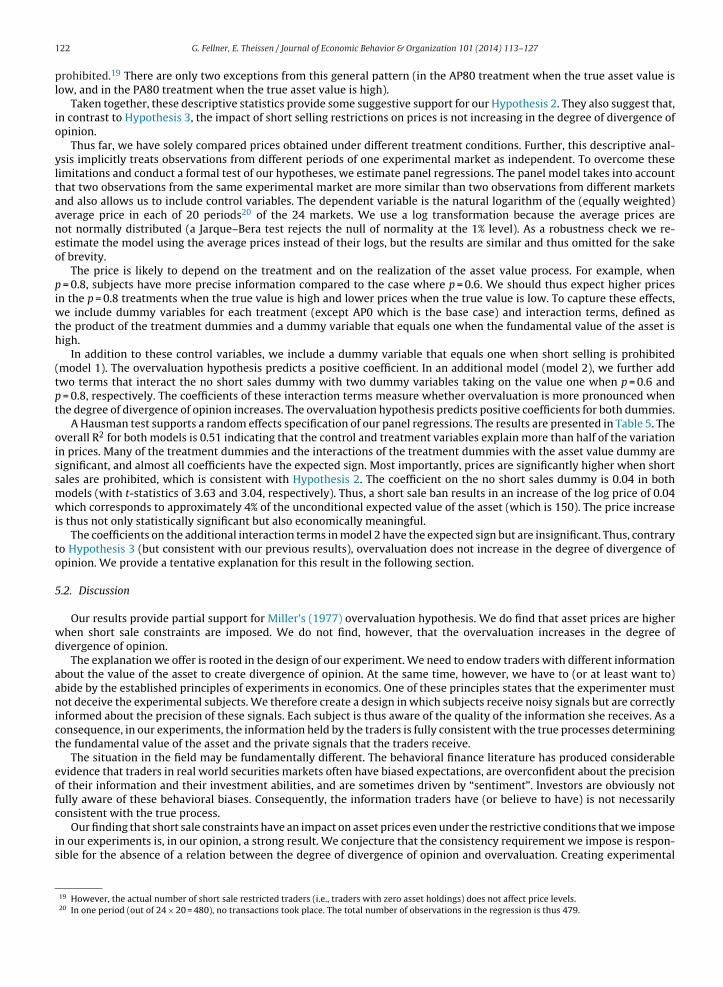
Thus far, we have solely compared prices obtained under different treatment conditions. Further, this descriptive anal-ysis implicitly treats observations from different periods of one experimental market as independent. To overcome theselimitations and conduct a formal test of our hypotheses, we estimate panel regressions. The panel model takes into accountthat two observations from the same experimental market are more similar than two observations from different marketsand also allows us to include control variables. The dependent variable is the natural logarithm of the (equally weighted)average price in each of 20 periods20 of the 24 markets. We use a log transformation because the average prices arenot normally distributed (a Jarque–Bera test rejects the null of normality at the 1% level). As a robustness check we re-estimate the model using the average prices instead of their logs, but the results are similar and thus omitted for the sakeof brevity.

The price is likely to depend on the treatment and on the realization of the asset value process. For example, whenp = 0.8, subjects have more precise information compared to the case where p = 0.6. We should thus expect higher pricesin the p = 0.8 treatments when the true value is high and lower prices when the true value is low. To capture these effects,we include dummy variables for each treatment (except AP0 which is the base case) and interaction terms, defined asthe product of the treatment dummies and a dummy variable that equals one when the fundamental value of the asset ishigh.

In addition to these control variables, we include a dummy variable that equals one when short selling is prohibited(model 1). The overvaluation hypothesis predicts a positive coefficient. In an additional model (model 2), we further addtwo terms that interact the no short sales dummy with two dummy variables taking on the value one when p = 0.6 andp = 0.8, respectively. The coefficients of these interaction terms measure whether overvaluation is more pronounced whenthe degree of divergence of opinion increases. The overvaluation hypothesis predicts positive coefficients for both dummies.

A Hausman test supports a random effects specification of our panel regressions. The results are presented in Table 5. Theoverall R2 for both models is 0.51 indicating that the control and treatment variables explain more than half of the variationin prices. Many of the treatment dummies and the interactions of the treatment dummies with the asset value dummy aresignificant, and almost all coefficients have the expected sign. Most importantly, prices are significantly higher when shortsales are prohibited, which is consistent with Hypothesis 2. The coefficient on the no short sales dummy is 0.04 in bothmodels (with t-statistics of 3.63 and 3.04, respectively). Thus, a short sale ban results in an increase of the log price of 0.04which corresponds to approximately 4% of the unconditional expected value of the asset (which is 150). The price increaseis thus not only statistically significant but also economically meaningful.

The coefficients on the additional interaction terms in model 2 have the expected sign but are insignificant. Thus, contraryto Hypothesis 3 (but consistent with our previous results), overvaluation does not increase in the degree of divergence ofopinion. We provide a tentative explanation for this result in the following section.

5.2. Discussion

Our results provide partial support for Miller’s (1977) overvaluation hypothesis. We do find that asset prices are higherwhen short sale constraints are imposed. We do not find, however, that the overvaluation increases in the degree ofdivergence of opinion.

The explanation we offer is rooted in the design of our experiment. We need to endow traders with different informationabout the value of the asset to create divergence of opinion. At the same time, however, we have to (or at least want to)abide by the established principles of experiments in economics. One of these principles states that the experimenter mustnot deceive the experimental subjects. We therefore create a design in which subjects receive noisy signals but are correctlyinformed about the precision of these signals. Each subject is thus aware of the quality of the information she receives. As aconsequence, in our experiments, the information held by the traders is fully consistent with the true processes determiningthe fundamental value of the asset and the private signals that the traders receive.

The situation in the field may be fundamentally different. The behavioral finance literature has produced considerableevidence that traders in real world securities markets often have biased expectations, are overconfident about the precisionof their information and their investment abilities, and are sometimes driven by “sentiment”. Investors are obviously notfully aware of these behavioral biases. Consequently, the information traders have (or believe to have) is not necessarilyconsistent with the true process.

Our finding that short sale constraints have an impact on asset prices even under the restrictive conditions that we imposein our experiments is, in our opinion, a strong result. We conjecture that the consistency requirement we impose is respon-sible for the absence of a relation between the degree of divergence of opinion and overvaluation. Creating experimental

19 However, the actual number of short sale restricted traders (i.e., traders with zero asset holdings) does not affect price levels.20 In one period (out of 24 × 20 = 480), no transactions took place. The total number of observations in the regression is thus 479.

G. Fellner, E. Theissen / Journal of Economic Behavior & Organization 101 (2014) 113–127 123

Table 5Price levels – panel regressions.

Model 1 Model 2

Coefficient z-Value Coefficient z-Value

Constant 4.94*** (356.87) 4.95*** (443.60)AP60 −0.01 (0.17) −0.01 (0.58)AP80 −0.09* (1.94) −0.09** (1.98)PA0 0.02 (0.42) 0.02 (0.43)PA60 0.05* (1.83) 0.04 (1.42)PA80 −0.13*** (4.79) −0.13*** (4.50)Value200 −0.01 (1.11) −0.01 (1.21)AP60*Value200 0.04*** (3.24) 0.04*** (3.12)AP80*Value200 0.27*** (4.14) 0.27*** (4.11)PA0*Value200 −0.00 (0.19) −0.00 (0.19)PA60*Value200 0.04** (2.45) 0.04** (2.35)PA80*Value200 0.40*** (9.55) 0.40*** (9.60)No short sales 0.04*** (3.63) 0.04*** (3.04)No short sales*div60 0.02 (0.53)No short sales*div80 0.00 (0.21)

R2 overall 0.510 0.510�u 0.068 0.068� i 0.095 0.095� 0.342 0.341No. obs. 479 479No. markets 24 24

The table shows the results of a random effects panel regression. The dependent variable is the log of the equally-weighted mean price of each period.We include control variables for the different treatment conditions and interactions between these control variables and a dummy that is equal to 1whenever the asset value is high (200). In model 1, we include a dummy variable that equals 1 when short selling is prohibited. In model 2, we furtherinclude interactions between the short selling dummy and dummy variables that equal 1 in those markets where p = 0.6 and p = 0.8 (denoted div 60 anddiv 80), respectively. The number of observations is 479 (24 markets, each with 20 periods; in one period no transaction took place). z-Values are based onheteroscedasticity-consistent standard errors.

* Significant at 10%.** Significant at 5%.

*** Significant at 1%.

Table 6Learning: First half versus second half.

Divergence of opinion Asset value Short sales allowed Short sales prohibited

P-A A-P P-A A-P

1st 2nd 1st 2nd 1st 2nd 1st 2nd

Benchmark 150.1 150.2 138.3 139.3 148.7 151.3 148.0 147.1

p = 0.6100 143.4 141.7 140.4 134.9 150.7 174.4 144.4 150.1200 153.4 163.1 144.6 149.6 154.1 154.2 148.0 152.3

p = 0.8100 110.7 105.5 130.8 134.2 148.8 153.7 119.2 132.5200 189.4 198.1 162.6 190.1 185.0 191.9 171.2 190.0

The table shows the medians of the average prices for the first half (periods 1–5) and the second half (periods 6–10) of the different treatment conditions.Te

ded

5

hro

A

he results are differentiated with respect to the degree of divergence of opinion (p = 0.6 and p = 0.8), the realization of the asset value process (with thexception of the benchmark case), the order of treatments (P-A and A-P) and the short selling condition (allowed and prohibited).

esigns that do not impose such a consistency requirement is a potential avenue for future research. The design of suchxperiments should, however, be closely guided by empirical evidence from the field. Otherwise the danger arises that theesign becomes arbitrary and produces arbitrary results.

.3. Learning

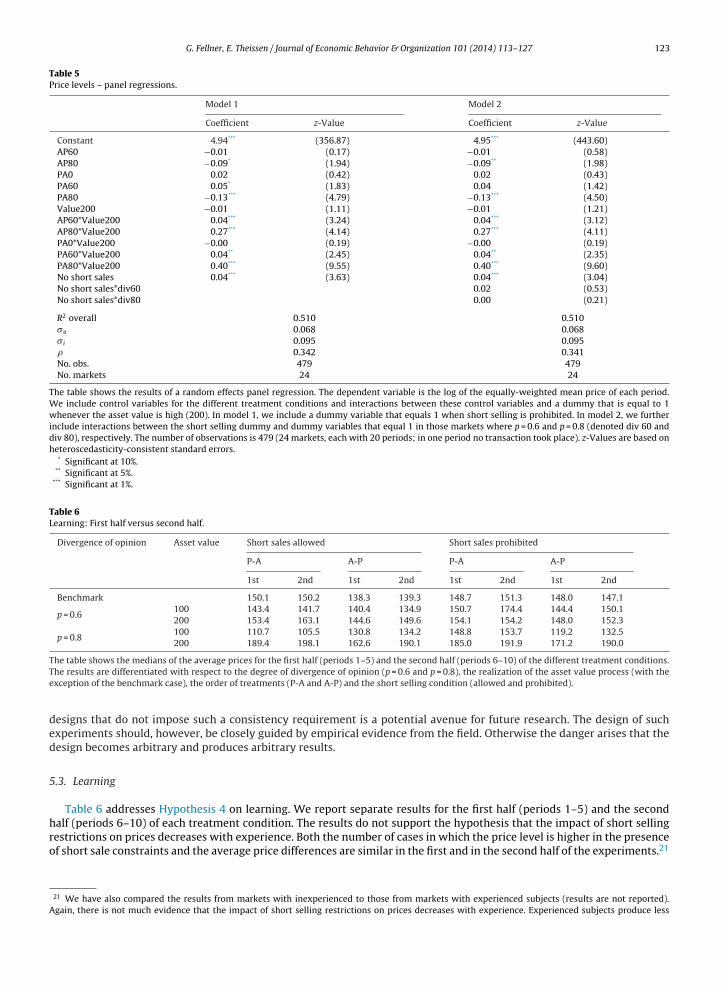
Table 6 addresses Hypothesis 4 on learning. We report separate results for the first half (periods 1–5) and the second

alf (periods 6–10) of each treatment condition. The results do not support the hypothesis that the impact of short sellingestrictions on prices decreases with experience. Both the number of cases in which the price level is higher in the presencef short sale constraints and the average price differences are similar in the first and in the second half of the experiments.21

21 We have also compared the results from markets with inexperienced to those from markets with experienced subjects (results are not reported).gain, there is not much evidence that the impact of short selling restrictions on prices decreases with experience. Experienced subjects produce less

124 G. Fellner, E. Theissen / Journal of Economic Behavior & Organization 101 (2014) 113–127

Table 7Trading volume – comparison of means.

Divergence of opinion Order of treatments Mean volume per period Median volume per period

Short sales allowed Short sales prohibited Short sales allowed Short sales prohibited

BenchmarkP-A 22.8 20.1 19.0 15.0A-P 21.7 8.9 18.5 8.0

p = 0.6P-A 18.6 15.8 18.0 15.0A-P 26.6 13.4 25.5 12.5

p = 0.8P-A 23.3 12.4 18.5 13.0A-P 24.3 10.2 18.5 9.0

Pooled 22.9 13.5 19.0 12.0

The table shows the mean and the median trading volume per period for the different treatment conditions. The last line shows results pooled over alltreatment conditions.

Table 8Trading volume – panel regressions.

Model 1 Model 2

Coefficient z-Value Coefficient z-Value

Constant 2.74*** (14.80) 2.73*** (12.97)AP60 0.31 (1.60) 0.29 (1.13)AP80 0.05 (0.18) 0.10 (0.30)PA0 0.35 (1.05) 0.35 (1.05)PA60 0.20 (0.87) 0.19 (0.70)PA80 0.16 (0.71) 0.21 (0.68)No short sales −0.48*** (5.07) −0.46*** (2.85)No short sales*div60 0.03 (0.12)No short sales*div80 −0.09 (0.40)

R2 overall 0.158 0.160�u 0.419 0.419� i 0.521 0.521� 0.393 0.393No. obs. 479 479No. markets 24 24

The table shows the results of a random effects panel regressions. The dependent variable is the log of trading volume (measured in numbers of shares) ineach period. We include control variables for the different treatment conditions. In model 1, we include a dummy variable that equals 1 when short sellingis prohibited. In model 2, we further include interactions between the short selling dummy and dummy variables that equal 1 in those markets where

p = 0.6 and p = 0.8 (denoted div 60 and div 80), respectively. The number of observations is 480 (24 markets, each with 20 periods). z-Values are based onheteroscedasticity-consistent standard errors.

*** Significant at 1%.

5.4. Trading volume and bid-ask spreads

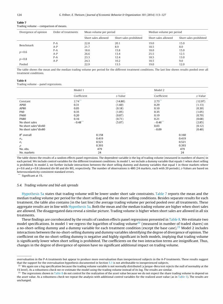
Hypothesis 5a states that trading volume will be lower under short sale constraints. Table 7 reports the mean and themedian trading volume per period for the short selling and the no short selling conditions. Besides separate results for eachtreatment, the table also contains (in the last line) the average trading volume per period pooled over all treatments. Theseaggregate results are in line with Hypothesis 5a. Both the mean and the median trading volume are higher when short salesare allowed. The disaggregated data reveal a similar picture. Trading volume is higher when short sales are allowed in all sixtreatments.

These findings are corroborated by the results of random effects panel regressions presented in Table 8. We estimate twomodel specifications. In model 1 we regress the logarithm of trading volume22 (measured in number of traded shares) ona no-short-selling dummy and a dummy variable for each treatment condition (except the base case).23 Model 2 includesinteractions between the no-short-selling dummy and dummy variables identifying the degree of divergence of opinion. The

coefficient on the no-short-selling dummy is negative and highly significant in both models, implying that trading volumeis significantly lower when short selling is prohibited. The coefficients on the two interaction terms are insignificant. Thus,changes in the degree of divergence of opinion have no significant additional impact on trading volume.

overvaluation in the P-A treatments but appear to produce more overvaluation than inexperienced subjects in the A-P treatments. These results suggestthat the support for the overvaluation hypothesis documented in Section 5.1 is not attributable to inexperienced subjects.

22 We again use a log specification because the trading volume variable is not normally distributed (a Jarque–Bera test rejects the null of normality at the1% level). As a robustness check we re-estimate the model using the trading volume instead of its log. The results are similar.

23 The regressions shown in Table 8 do not control for the realization of the asset value because we do not expect the share trading volume to depend onthe asset value. As a robustness check we repeat the analysis with additional control variables for the realized asset value (as in Table 5). The results areunchanged.

G. Fellner, E. Theissen / Journal of Economic Behavior & Organization 101 (2014) 113–127 125

Table 9Bid-ask spreads – comparison of means.

Divergence of opinion Order of treatments Mean quoted spread Median quoted spread

Short sales allowed Short sales prohibited Short sales allowed Short sales prohibited

Panel A: mean and median quoted spreadsBenchmark P-A 13.9 28.4 8.1 24.7

A-P 20.3 15.9 15.5 14.4Pooled 17.1 22.2 10.6 19.0

p = 0.6 P-A 22.6 30.6 21.7 33.2A-P 40.3 29.6 30.5 26.0Pooled 31.3 30.1 23.8 32.2

p = 0.8 P-A 19.8 33.8 15.6 33.9A-P 41.5 38.7 41.5 36.3Pooled 30.7 36.3 27.2 35.5

Divergence of opinion Order of treatments Mean effective spread Median effective spread

Short sales allowed Short sales prohibited Short sales allowed Short sales prohibited

Panel B: mean and median effective spreadsBenchmark P-A 9.8 23.2 7.1 17.9

A-P 15.1 8.8 9.1 6.0Pooled 12.5 16.0 7.6 10.5

p = 0.6 P-A 16.1 23.0 14.1 22.2A-P 36.2 23.0 22.9 17.2Pooled 26.0 23.0 18.2 18.4

p = 0.8 P-A 21.0 29.0 16.2 26.8A-P 30.7 26.1 31.6 23.2Pooled 25.9 27.6 23.7 25.3

TT(

Ar(

Ata

tqqttfis

lTs

pow

nTrp

he table shows average bid-ask spreads for the different treatment conditions. Panel A shows mean quoted spreads, Panel B shows mean effective spreads.he results are differentiated with respect to the degree of divergence of opinion, the order of treatments (P-A and A-P) and the short selling conditionallowed and prohibited).

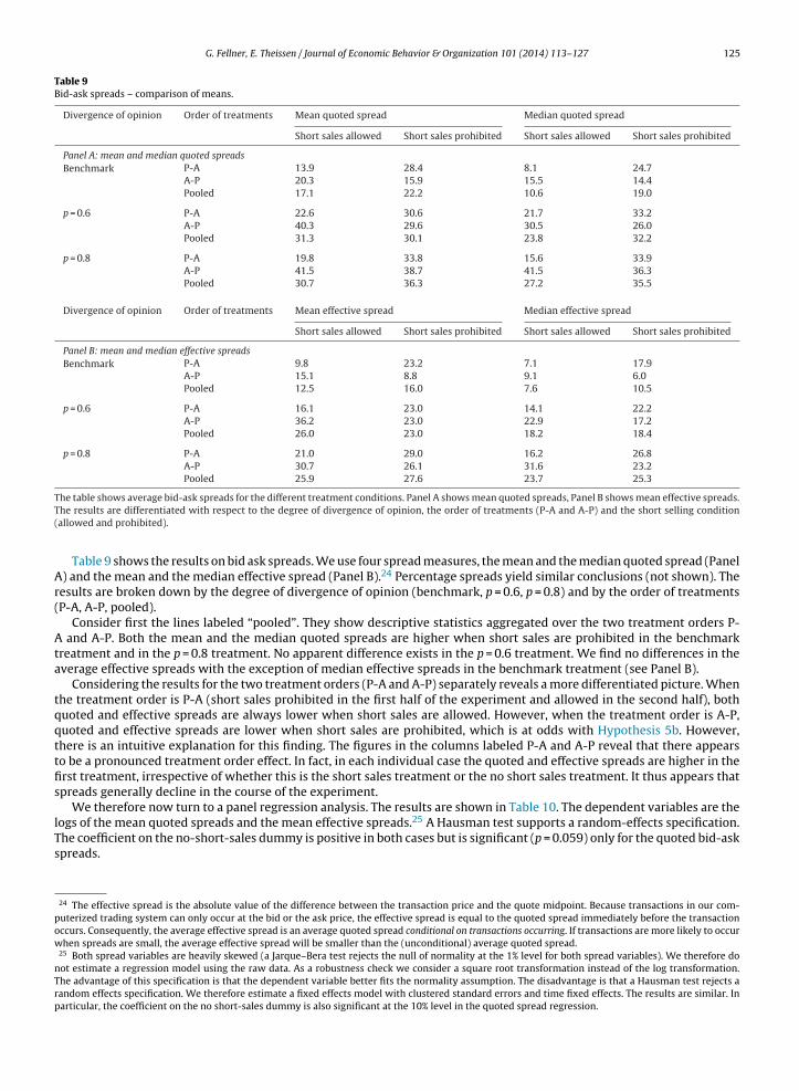
Table 9 shows the results on bid ask spreads. We use four spread measures, the mean and the median quoted spread (Panel) and the mean and the median effective spread (Panel B).24 Percentage spreads yield similar conclusions (not shown). Theesults are broken down by the degree of divergence of opinion (benchmark, p = 0.6, p = 0.8) and by the order of treatmentsP-A, A-P, pooled).

Consider first the lines labeled “pooled”. They show descriptive statistics aggregated over the two treatment orders P- and A-P. Both the mean and the median quoted spreads are higher when short sales are prohibited in the benchmark

reatment and in the p = 0.8 treatment. No apparent difference exists in the p = 0.6 treatment. We find no differences in theverage effective spreads with the exception of median effective spreads in the benchmark treatment (see Panel B).

Considering the results for the two treatment orders (P-A and A-P) separately reveals a more differentiated picture. Whenhe treatment order is P-A (short sales prohibited in the first half of the experiment and allowed in the second half), bothuoted and effective spreads are always lower when short sales are allowed. However, when the treatment order is A-P,uoted and effective spreads are lower when short sales are prohibited, which is at odds with Hypothesis 5b. However,here is an intuitive explanation for this finding. The figures in the columns labeled P-A and A-P reveal that there appearso be a pronounced treatment order effect. In fact, in each individual case the quoted and effective spreads are higher in therst treatment, irrespective of whether this is the short sales treatment or the no short sales treatment. It thus appears thatpreads generally decline in the course of the experiment.

We therefore now turn to a panel regression analysis. The results are shown in Table 10. The dependent variables are the

ogs of the mean quoted spreads and the mean effective spreads.25 A Hausman test supports a random-effects specification.he coefficient on the no-short-sales dummy is positive in both cases but is significant (p = 0.059) only for the quoted bid-askpreads.

24 The effective spread is the absolute value of the difference between the transaction price and the quote midpoint. Because transactions in our com-uterized trading system can only occur at the bid or the ask price, the effective spread is equal to the quoted spread immediately before the transactionccurs. Consequently, the average effective spread is an average quoted spread conditional on transactions occurring. If transactions are more likely to occurhen spreads are small, the average effective spread will be smaller than the (unconditional) average quoted spread.

25 Both spread variables are heavily skewed (a Jarque–Bera test rejects the null of normality at the 1% level for both spread variables). We therefore doot estimate a regression model using the raw data. As a robustness check we consider a square root transformation instead of the log transformation.he advantage of this specification is that the dependent variable better fits the normality assumption. The disadvantage is that a Hausman test rejects aandom effects specification. We therefore estimate a fixed effects model with clustered standard errors and time fixed effects. The results are similar. Inarticular, the coefficient on the no short-sales dummy is also significant at the 10% level in the quoted spread regression.

126 G. Fellner, E. Theissen / Journal of Economic Behavior & Organization 101 (2014) 113–127

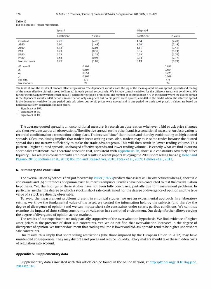
Table 10Bid-ask spreads – panel regressions.

Spread Effspread

Coefficient z-Value Coefficient z-Value

Constant 2.27*** (4.26) 1.94*** (4.49)AP60 0.90 (1.48) 1.09** (2.14)AP80 1.12** (2.04) 1.11** (2.41)PA0 0.23 (0.39) 0.35 (0.73)PA60 0.73 (1.32) 0.78* (1.76)PA80 0.53 (0.98) 0.94** (2.17)No short sales 0.29* (1.89) 0.13 (0.79)

R2 overall 0.193 0.186�u 0.607 0.554� i 0.651 0.725� 0.465 0.368No. obs. 479 478No. markets 24 24

The table shows the results of random effects regressions. The dependent variables are the log of the mean quoted bid-ask spread (spread) and the logof the mean effective bid-ask spread (effspread) in each period, respectively. We include control variables for the different treatment conditions. Wefurther include a dummy variable that equals 1 when short selling is prohibited. The number of observations is 479 in the model where the quoted spreadis the dependent variable (480 periods; in one period only ask prices but no bid prices were quoted) and 478 in the model where the effective spreadis the dependent variable (in one period only ask prices but no bid prices were quoted and in one period no trade took place). t-Values are based onheteroscedasticity-consistent standard errors.

* Significant at 10%.

** Significant at 5%.

*** Significant at 1%.

The average quoted spread is an unconditional measure. It records an observation whenever a bid or ask price changesand then averages across all observations. The effective spread, on the other hand, is a conditional measure. An observation isrecorded conditional on a transaction taking place. Traders can “time” their trades and thereby avoid trading on high quotedspreads. Of course, timing implies that traders incur waiting costs. Also, traders may miss some trades because the quotedspread does not narrow sufficiently to make the trade advantageous. This will then result in lower trading volume. Thispattern – higher quoted spreads, unchanged effective spreads and lower trading volume – is exactly what we find in our noshort-sales treatments. We therefore conclude that, consistent with Hypothesis 5b, short sale constraints adversely affectliquidity. This result is consistent with empirical results in recent papers studying the 2008 short selling ban (e.g. Beber andPagano, 2013; Boehmer et al., 2013; Boulton and Braga-Alves, 2010; Fotak et al., 2009; Helmes et al., 2011).

6. Summary and conclusion

The overvaluation hypothesis first put forward by Miller (1977) predicts that assets will be overvalued when (a) short saleconstraints and (b) differences of opinion exist. Numerous empirical studies have been conducted to test the overvaluationhypothesis. Yet, the findings of these studies have not been fully conclusive, partially due to measurement problems. Inparticular, neither the degree to which a stock is short sale constrained nor the degree of divergence of opinion and the truevalue of a stock are directly observable.

To avoid the measurement problems present in empirical studies, we use an experimental approach. In a laboratorysetting, we know the fundamental value of the asset, we control the information held by the subjects (and thereby thedegree of divergence of opinion) and we can impose short sale constraints under ceteris paribus conditions. We can thusexamine the impact of short selling constraints on valuation in a controlled environment. Our design further allows varyingthe degree of divergence of opinion across markets.

The results of our experiment are only partially supportive of the overvaluation hypothesis. We find evidence of higherasset prices in the presence of short sale constraints. Yet, we do not find that overvaluation increases in the degree ofdivergence of opinion. We further document that trading volume is lower and bid-ask spreads tend to be higher under shortsale constraints.

Our results thus imply that short selling restrictions (like those imposed by the European Union in 2012) may haveunintended consequences. They may distort asset prices and reduce liquidity. Policy makers should take these hidden costsof regulation into account.

Appendix A. Supplementary data

Supplementary data associated with this article can be found, in the online version, at http://dx.doi.org/10.1016/j.jebo.2014.02.010.

R

A

A

AAAA

ABBB

BBB

BBBBBBCCCDD

DD

DDDDDDDDFFFF

GG

GGG

H

HH

H

HJJJKK

M

MNO

PRSS

G. Fellner, E. Theissen / Journal of Economic Behavior & Organization 101 (2014) 113–127 127

eferences

ckert, L., Charupat, N., Church, B., Deaves, R., 2002. Bubbles in experimental asset markets: Irrational exuberance no more. Federal Reserve Bank of AtlantaWorking Paper 2002-24, December.

itken, M., Frino, A., McCorry, M., Swan, P., 1998. Short sales are almost instantaneously bad news: Evidence from the Australian stock exchange. Journalof Finance 53, 2205–2223.

squith, P., Meulbroek, L., 1995. An empirical investigation of short interest. Working paper. Harvard University.squith, Paul, Pathak, P., Ritter, J., 2005. Short interest, institutional ownership and stock returns. Journal of Financial Economics 78, 243–276.u, A., Doukas, J., Onayev, Z., 2009. Daily short interest, idiosyncratic risk, and stock returns. Journal of Financial Markets 12, 290–316.utore, D., Billingsley, R., Kovacs, T., 2011a. The 2008 short sale ban: liquidity, dispersion of opinions, and the cross-section of returns on U.S. financial

stocks. Journal of Banking and Finance 35, 2252–2266.utore, D., Boulton, Th., Braga-Alves, M., 2011b. Failures to deliver, short sale constraints, and stock overvaluation. AFA 2012 Chicago Meetings Paper.attalio, R., Schultz, P., 2006. Options and the bubble. Journal of Finance 61, 2071–2102.eber, A., Pagano, M., 2013. Short selling bans around the world: Evidence from the 2007–09 crisis. Journal of Finance 68, 343–381.erkman, H., Dimitrov, V., Jain, P., Koch, P., Tice, S., 2009. Sell on news: difference of opinion, short-sales constraints, and returns around earnings

announcements. Journal of Financial Economics 92, 376–399.erkman, H., Koch, P., 2008. Disagreement, short sale constraints, and speculative trading before earnings announcements. Working Paper, June.hojraj, S., Bloomfield, R., Tayler, W., 2009. Margin trading, overpricing, and synchronization risk. Review of Financial Studies 22, 2059–2085.oehme, R., Danielsen, B., Sorescu, S., 2006. Short sale constraints, difference of opinion, and overvaluation. Journal of Financial and Quantitative Analysis

41, 455–487.oehmer, E., Jones, Ch., Zhang, X., 2008. Which shorts are informed? Journal of Finance 63, 491–527.oehmer, E., Huszar, Z., Jordan, B., 2010. The good news in short interest. Journal of Financial Economic 96, 80–97.oehmer, E., Jones, C., Zhang, X., 2013. Shackling short sellers: The 2008 shorting ban. Review of Financial Studies 26, 1363–1400.oulton, T., Braga-Alves, M., 2010. The skinny on the 2008 naked short-sale restrictions. Journal of Financial Markets 13, 397–421.rent, A., Morse, D., Stice, E., 1990. Short interest: explanations and tests. Journal of Financial and Quantitative Analysis 25, 273–289.ris, A., Goetzmann, W., Zhu, N., 2007. Efficiency and the bear: short sales and markets around the world. Journal of Finance 62, 1029–1079.hang, E., Cheng, J., Yu, Y., 2007. Short-sales constraints and price discovery: evidence from the Hong Kong market. Journal of Finance 62, 2097–2121.haroenrook, A., Daouk, H., 2009. A study of market-wide short-selling restrictions. Working Paper Cornell University., pp. 2009–2021.ohen, L., Diether, K., Malloy, Ch., 2007. Supply and demand shifts in the shorting market. Journal of Finance 62, 2061–2096.’Avolio, G., 2002. The market for borrowing stock. Journal of Financial Economics 66, 271–306.anielsen, B.R., Sorescu, S.M., 2001. Why do option introductions depress stock prices? A study of diminishing short-sale constraints. Journal of Financial

and Quantitative Analysis 36, 451–484.echow, P.M., Hutton, A.P., Meulbroek, L., Sloan, R.G., 2001. Short-sellers, fundamental analysis and stock returns. Journal of Financial Economics 61, 77–106.esai, H., Ramesh, K., Thiagarajan, S.R., Balachandran, B.V., 2002. An investigation of the informational role of short interest in the NASDAQ market. Journal

of Finance 57, 2263–2287.iamond, D., Verrecchia, R., 1987. Constraints on short-selling and asset price adjustment to private information. Journal of Financial Economics 18, 277–311.iether, K., Lee, K.-H., Werner, I., 2005. Can short sellers predict returns? Daily evidence. Charles A. Dice Center Working Paper No. 2005-15, July.iether, K., Lee, K.-H., Werner, I., 2009a. Short-sale strategies and return predictability. Review of Financial Studies 22, 575–607.iether, K., Lee, K.-H., Werner, I., 2009b. It’s SHO time! Short-sale price tests and market quality. Journal of Finance 64, 37–73.iether, K., Malloy, C.J., Scherbina, A., 2002. Differences of opinion and the cross-section of stock returns. Journal of Finance 57, 2113–2141.iether, K., Werner, I., 2009. When constraints bind. Charles A. Dice Center Working Paper No. 2009-15, July.ong, M., Michel, J.-S., 2008. Does investor heterogeneity lead to IPO overvaluation? Working Paper, March.uffie, D., Garleanu, N., Pedersen, L.H., 2002. Securities lending, shorting and pricing. Journal of Financial Economics 66, 307–339.iglewski, S., Webb, G.P., 1993. Options, short sales, and market completeness. Journal of Finance 48, 761–777.ischbacher, U., 2007. z-Tree: Zurich toolbox for ready-made economic experiments. Experimental Economics 10, 171–178.otak, V., Raman, V., Yadav, P., 2009. Naked Short Selling: The Emperor’s New Clothes? Working Paper, University of Oklahoma, May.rancis, J., Venkatachalam, M., Zhang, Y., 2005. Do short sellers convey information about changes in fundamentals or risk? Working Paper, Duke University,

September.agnon, L., Witmer, J., 2010. Short Changed? The Market’s Reaction to the Short Sale Ban of 2008. Bank of Canada Working Paper 2009-23, October.allmeyer, M., Hollifield, B., 2008. An examination of heterogeneous beliefs with a short-sale constraint in a dynamic economy. Review of Finance 12,

323–364.reenwood, R., 2009. Trading restrictions and stock prices. Review of Financial Studies 22, 509–539.opalan, M., 2003. Short Constraints, Difference of Opinion and Stock Returns. Working Paper, Duke University, December.reiner, B., 2004. The Online Recruitment System ORSEE 2.0 – A Guide for the Organization of Experiments in Economics. Working Paper Series in Economics

10, University of Cologne.arris, L., Namvar, E., Pillips, B., 2013. Price inflation and wealth transfer during the 2008 SEC short-sale ban. Journal of Investment Management 11, second

quarter.aruvy, E., Noussair, Ch, 2006. The effect of short selling on bubbles and crashes in experimental spot asset markets. Journal of Finance 61, 1119–1157.auser, F., Huber, J., 2012. Short-selling constraints as cause for price distortions: an experimental study. Journal of International Money and Finance 31,

1279–1298.elmes, U., Henker, J., Henker, T., 2011. The effect of the ban on short selling on market efficiency and volatility. 2011 Financial Management Association

(FMA) Annual Meeting, 1–54.ong, H., Stein, J., 2003. Differences of opinion, short sales constraints and market crashes. Review of Financial Studies 16, 487–525.

iang, D., 2005. Overconfidence, Short-sale Constraints, and Stock Valuation. Working Paper, Ohio State University, September.ohnson, T., 2004. Forecast dispersion and the cross section of expected returns. Journal of Finance 59, 1957–1978.ones, C.M., Lamont, O.A., 2002. Short sale constraints and stock returns. Journal of Financial Economics 66, 207–239.aplan, S., Moskowitz, T., Sensoy, B., 2013. The effects of stock lending on security prices: an experiment. Journal of Finance 68, 1891–1936.ing, R., Smith, V., Williams, A., Van Boening, M., 1993. The robustness of bubbles and crashes in experimental stock markets. In: Prigogine, I., Day, R., Chen,

P. (Eds.), Nonlinear Dynamics and Evolutionary Economics. Oxford University Press, Oxford.ayhew, S., Mihov, V., 2004. Short Sale Constraints, Overvaluation and the Introduction of Options. Working Paper, SEC and Texas Christian University,

December.iller, E., 1977. Risk, uncertainty, and divergence of opinion. Journal of Finance 32, 1151–1168.agel, S., 2005. Short sales, institutional investors and the cross-section of stock returns. Journal of Financial Economics 78, 277–309.fek, E., Richardson, M., Whitelaw, R., 2004. Limited arbitrage and short sale restrictions: evidence from the options market. Journal of Financial Economics

74, 305–342.hillips, B., 2011. Options, short-sale constraints and market efficiency: a new perspective. Journal of Banking and Finance 35, 430–442.eed, A., 2007. Costly short-selling and stock price adjustment to earnings announcements. Working Paper, University of North Carolina, July.cheinkman, J., Xiong, W., 2003. Overconfidence and speculative bubbles. Journal of Political Economy 111, 1183–1219.mith, V., Suchanek, G., Williams, A., 1988. Bubbles, crashes, and endogenous expectations in experimental spot asset markets. Econometrica 56, 1119–1151.