SHORT-RUN FLUCTUATIONS

David Romer

University of California, Berkeley

August 2002

Copyright 2002 by David Romer

i

CONTENTS

Preface iv

I The IS-MP Model 1

I-1 Monetary Policy and the MP Curve 1

I-2 Using the IS-MP Model to Understand Short-Run Fluctuations 3

An Increase in Government Purchases 4

A Shift to Tighter Monetary Policy 5

Fiscal and Monetary Policy Together: The Policy Mix 5

A Fall in Consumer Confidence 7

I-3 The Money Market and the Central Bank's Control of the Real Interest Rate 9

The Money Market 9

The Money Supply and the Real Interest Rate with Completely Sticky Prices 11

The Money Supply and the Real Interest Rate with Price Adjustment 13

Problems 18

ii

II The Open Economy 20

II-1 Short-Run Fluctuations with Floating Exchange Rates 21

Planned Expenditure in an Open Economy 21

Net Exports and Net Foreign Investment 23

The IS Curve with Floating Exchange Rates 25

The Determination of Net Exports and the Exchange Rate 27

II-2 Using the Model of Floating Exchange Rates 28

Fiscal Policy 28

Monetary Policy 30

Trade Policy 30

II-3 Short-Run Fluctuations with Fixed Exchange Rates 32

The Mechanics of Fixing the Exchange Rate 32

The IS Curve with Fixed Exchange Rates 34

The Reserve Loss and Limits on Policy 36

II-4 Using the Model of Fixed Exchange Rates 37

Fiscal Policy 37

Monetary Policy 38

Trade Policy 38

A Fall in Export Demand 39

Devaluation 40

Problems 40

iii

III Aggregate Supply 42

III-1 Extending the Model to Include Aggregate Supply 42

The Behavior of Inflation 42

The Effect of Inflation on Monetary Policy 45

The AD-IA Diagram 46

The Behavior of Output and Inflation over Time 47

III-2 Changes on the Aggregate Demand Side of the Economy 49

Fiscal Policy 49

Monetary Policy 54

Monetary Policy and Inflation in the Long Run 56

III-3 Changes on the Aggregate Supply Side of the Economy 59

Inflation Shocks and Supply Shocks 59

The Effects of an Inflation Shock 62

The Effects of a Supply Shock 63

Inflation Expectations and Inflation Shocks 64

Problems 67

1 N. Gregory Mankiw, Macroeconomics, fifth edition (New York: Worth Publishers,2003).

2 David Romer, "Keynesian Macroeconomics without the LM Curve." Journal ofEconomic Perspectives 14 (Spring 2000): 149-169.

iv

PREFACE

This document presents a model of the determination of output, unemployment,

inflation, and other macroeconomic variables in the short run at a level suitable for students

taking intermediate macroeconomics. The model is based on an assumption about how

central banks conduct monetary policy that differs from the one made in most intermediate

macroeconomics textbooks. The document is designed to be used in conjunction with

standard textbooks by instructors and students who believe that the new approach provides a

more realistic and powerful way of analyzing short-run fluctuations.

I have designed the document to work most closely with N. Gregory Mankiw's

textbook, which I refer to simply as "Mankiw."1 The material here can take the place of the

material in Mankiw starting with Section 10-2 and ending with Chapter 13. The notation is

the same as Mankiw's, and I refer to other parts of Mankiw when they are relevant. But I

believe the document can be used with other intermediate macroeconomics textbooks

without great difficulty.

In a separate paper, I compare the new approach with the usual one and explain why I

believe it is preferable.2 This document, however, simply presents the new approach and

shows how to use it. In addition, the presentation here is more skeletal than that in standard

v

textbooks. The document covers the basics, but contains relatively few applications,

summaries, and problems.

I am indebted to Christina Romer and Patrick McCabe for helpful comments and

discussions, and to my students for their encouragement, patience, and feedback on earlier

versions of this material.

The document may be downloaded, reproduced, and distributed freely by instructors

and students as long as credit is given to the author and the copyright notice on the title page

is included.

1 See Mankiw, Section 10-1.

1

I The IS-MP Model

I-1 Monetary Policy and the MP Curve

You have already learned about the IS curve, shown in Figure I-1.1 The curve shows

the relationship between the real interest rate and equilibrium output in the goods market.

An increase in the interest rate reduces planned investment. As a result, it reduces planned

expenditure at a given level of output. Thus the planned expenditure line in the Keynesian

cross diagram shifts down, and so the level of output at which planned expenditure equals

output falls. This negative relationship between the interest rate and output is known as the

IS curve.

The IS curve by itself does not tell us what either the interest rate or output is. We

know that the economy must be somewhere on the curve, but we do not know where. To pin

down where, we need a second relationship between the interest rate and output.

This second relationship comes from the conduct of monetary policy. Monetary

policy is conducted by the economy's central bank (the Federal Reserve in the case of the

United States). A key feature of how the central bank conducts monetary policy is how it

responds to changes in output:

2

When output rises, the central bank raises the real interest rate. When output

falls, the central bank lowers the real interest rate.

We can express this characteristic of monetary policy in the form of an equation:

r = r(Y). (I-1)

When output, Y, rises, the central bank raises the real interest rate, r. Thus r(Y) is an

increasing function.

We can also depict this relationship using a diagram. The fact that the central bank

raises the real interest rate when output rises means that there is an upward-sloping

relationship between output and the interest rate. This curve is known as the MP curve. It is

shown in Figure I-2.

Ultimately, the fact that the central bank raises the interest rate when output rises and

lowers it when output falls stems from policymakers' goals for output and inflation. All else

equal, central bankers prefer that output be higher. Thus when output declines, they reduce

the interest rate in order to increase the demand for goods and thereby stem the fall in

output. But the central bank cannot just keep cutting the interest rate and raising the demand

for goods further and further. As we will see in Section III, when output is above its natural

rate, so that firms are operating at above their usual capacities, inflation usually begins to

rise. Since central bankers want to keep inflation from becoming too high, they raise the

interest rate when output rises. It is these twin concerns about output and inflation that cause

the central bank to make the real interest rate an increasing function of output.

3

This description of how the central bank conducts monetary policy leaves two issues

unresolved. The first issue is how the central bank controls the real interest rate. Central

banks do not set the interest rate by decree. Instead they adjust the money supply to cause

the interest rate behave in the way they want. We will discuss the specifics of how they do

this in Section I-3. For most of our analysis, however, we will simply take as given that the

central bank can control the interest rate, and that it does so in a way that makes it an

increasing function of output.

The second unresolved issue concerns shifts of the MP curve. In Section III, we will

see that the central bank adjusts the real interest rate in response not only to output, but also

to inflation. An increase in inflation causes the central bank to choose a higher interest rate

at a given level of output than before. That is, it causes the MP curve to shift up. Thus, the

MP curve shows the relationship between output and the interest rate at a given time, but

changes in inflation cause the curve to shift over time.

I-2 Using the IS-MP Model to Understand Short-Run Fluctuations

We can now bring the IS and MP curves together. They are shown in the IS-MP

diagram in Figure I-3. The point where the two curves intersect shows the real interest rate

and output in the economy. At this point, planned expenditure equals output, and the central

bank is choosing the interest rate according to its policy rule. The IS-MP diagram is our

basic tool for analyzing how the interest rate and output are determined in the short run. We

can therefore use it to analyze how various economic developments affect these two

4

variables.

An Increase in Government Purchases

Suppose that government purchases increase. Government purchases are a

component of planned expenditure. Thus the rise in purchases affects the IS curve. To see

how, we use the Keynesian cross diagram shown in Figure I-4. Recall that the Keynesian

cross shows planned expenditure as a function of output for a given level of the real interest

rate. Thus the intersection of the planned expenditure line and the 45-degree line shows

equilibrium output for a given interest rate. That is, it determines a point on the IS curve.

The increase in government purchases raises planned expenditure at a given level of

income. Thus, as the figure shows, it shifts the planned expenditure line up. This increases

the equilibrium level of income at the interest rate assumed in drawing the diagram.

In terms of the IS-MP diagram, this analysis shows us that at a given interest rate,

equilibrium income is higher than before. That is, the IS curve shifts to the right. The

central bank's rule for choosing the interest rate as a function of output is unchanged. Thus

the MP curve does not shift. This information is summarized in Figure I-5.

The figure shows that at the intersection of the new IS curve and the MP curve, both

the interest rate and output are higher than before. Thus the figure shows that an increase in

government purchases raises both the interest rate and output in the short run.

We can also determine how the increase in government purchases affects the other

components of output. The increase in the interest rate reduces investment. Thus

2 See Section 3-4 of Mankiw for the long-run effects of a change in governmentpurchases.

5

government purchases crowd out investment in the short run, just as they do in the long run.2

Since consumption is an increasing function of disposable income, on the other hand, the

increase in income resulting from the rise in government purchases raises consumption.

A Shift to Tighter Monetary Policy

We can also analyze a change in monetary policy. Specifically, suppose the central

bank changes its monetary policy rule so that it chooses a higher level of the real interest rate

at a given level of output than before. This move to tighter monetary policy corresponds to

an upward shift of the MP curve. The IS curve is not affected: equilibrium output at a given

interest rate is unchanged. This information is summarized in Figure I-6. The figure shows

that the shift to tighter monetary policy raises the interest rate and lowers output in the short

run.

We can again determine the effects of the policy change on the components of

output. The increase in the interest rate reduces investment, and the decline in income

reduces consumption. Since government purchases are an exogenous variable of our model,

they are unchanged.

Fiscal and Monetary Policy Together: The Policy Mix

Changes in fiscal and monetary policy need not occur in isolation. There are many

cases when both policies change at the same time. There can be deliberate coordination

between the two sets of policymakers, one can react to the other's actions, or outside

6

developments can prompt independent responses by both.

When fiscal and monetary policies both change, the IS and MP curves both move.

Depending on such factors as the directions and sizes of moves, there can be almost any

combination of changes in the interest rate and output. A particularly interesting case to

consider is when the two policies change in a way that leaves output unchanged. For

concreteness, suppose that Congress and the President raise taxes, and at the same time the

Federal Reserve changes its rule for setting the interest rate as a function of output by

enough to keep output at its initial level.

These assumptions provide a reasonably good description of some developments in

the U.S. economy in the early 1990s under Presidents Bush and Clinton. Motivated by a

desire to reduce the budget deficit, Congress and the President made various changes to the

budget to increase taxes and to reduce transfer payments and government purchases. The

Federal Reserve did not want these changes to reduce output. It therefore lowered the

interest rate at a given level of output to keep output at roughly the same level as before.

Figure I-7 shows the effects of these developments. The increase in taxes shifts the

IS curve to the left. The reasoning is essentially the reverse of our earlier analysis of a rise

in government purchases. Since consumption depends on disposable income, Y-T, the

increase in T reduces consumption at a given Y. Thus it shifts the planned expenditure line

in the Keynesian cross diagram down, and so reduces equilibrium output at a given interest

rate. And the Federal Reserve's decision to reduce the interest rate at a given level of output

causes the MP curve to shift down. By assumption, the new IS and MP curves cross at the

same level of output as before.

7

Although this simultaneous change in fiscal and monetary policy does not change

overall output, it does change the composition of output. With income unchanged and taxes

higher than before, disposable income is lower than before; thus consumption is lower than

before. And as Figure I-7 shows, the combination of contractionary fiscal policy and

expansionary monetary policy lowers the interest rate. Thus investment rises. Finally,

government purchases are again unchanged by assumption.

This analysis shows how the coordinated use of fiscal and monetary policy can keep

policies to lower the budget deficit from reducing aggregate output. It also shows how

policy coordination can shift the composition of output away from consumption and toward

investment.

A Fall in Consumer Confidence

So far, the only sources of short-run economic fluctuations we have considered are

changes in government policies. But developments in the private economy can also cause

fluctuations. For our final example, we consider the effects of a decline in consumer

confidence. That is, we suppose that for some reason consumers become more worried

about the future, and that they therefore consume less and save more at a given level of

disposable income than before.

This fall in consumer confidence shifts the IS curve; the analysis is similar to the

analysis of a tax increase. Figure I-8 shows the effects of the shift. The economy moves

down along the MP curve. Thus the real interest rate and output both fall.

Shifts in consumer confidence are an important source of short-run fluctuations. To

give one example, Iraq's invasion of Kuwait and other developments caused a sharp fall in

3 See Section 14-1 of Mankiw for more on why policymakers' control of the economy isnot immediate or perfect.

4 Christina D. Romer, "The Great Crash and the Onset of the Great Depression,"Quarterly Journal of Economics 105 (May 1990), pp. 597-624.

8

consumer confidence in the United States in the summer of 1990. This fall in confidence

shifted the IS curve to the left. In principle, a rapid response by monetary policymakers

could have shifted the MP curve down and kept output from falling. Alternatively, rapid

increases in government purchases or decreases in taxes could have kept the IS curve from

shifting at all. In practice, however, policymakers did not become aware of the fall in

consumer confidence quickly enough to take corrective action. The result was that the

United States entered a recession.3

A more important example of a downward shift in the consumption function occurred

in the United States in 1929. The stock market crash of October 1929, coming after almost a

decade of rapidly rising stock prices and enormous increases in participation in the stock

market, created tremendous uncertainty among consumers. As a result, they put off making

major purchases to see what developed. Thus, consumption at a given level of income fell

sharply. The resulting shift of the IS curve was an important factor in changing what was at

that point only a mild recession into the enormous downturn that became known as the Great

Depression.4

5 See Section 4-5 of Mankiw.

9

I-3 The Money Market and the Central Bank's Control of the Real Interest

Rate

The Money Market

The assumption that the central bank can change the real interest rate is crucial to the

existence of the MP curve. In this section, we will investigate how the central bank is able

to do this. We will see that what gives it this ability is its control of the money supply.

Thus, we will examine the market for money.

Equilibrium in the money market occurs when the supply of real money balances

equals the demand. The supply of real balances is simply the quantity of money measured in

terms of the amount of goods it can buy. That is, it equals the dollar amount of money, M,

divided by the price of goods in terms of dollars, P: the supply of real money balances is

M/P.

Recall from your earlier analysis of money and inflation that there are two key

determinants of the demand for real balances. The first is income, Y. When income is

higher, people make more transactions, and so they want to hold a greater quantity of real

balances. The second is the nominal interest rate, i. Money does not earn any interest, while

other assets earn the nominal interest rate. The opportunity cost of holding money is thus

the nominal interest rate. When the nominal interest rate is higher, individuals want to hold

a smaller quantity of real balances.5

This discussion shows that the condition for the supply and demand of real balances

10

(I-2)

to be equal is

where L is a function that tells us the demand for real balances given the nominal interest

rate and income. The function is decreasing in the interest rate and increasing in income.

We want to know whether the central bank can influence the real interest rate. To

address this question, it helps to use the fact that, by definition, the real interest rate is the

difference between the nominal interest rate and expected inflation: r = i - Be, where Be

denotes expected inflation. This equation implies that the nominal rate equals the real rate

plus expected inflation: i = r + Be. Substituting this expression for the nominal rate into the

condition for equilibrium in the money market gives us

Equation (I-2) is the equation we will use to see how the central bank influences the real

interest rate.

The central bank controls the nominal money supply directly. But when it changes

the nominal money supply, the price level and expected inflation may also change. Thus it

is not obvious how a change in the nominal money supply affects supply and demand in the

money market. Our strategy will be to tackle this question in two steps. We will first

11

consider what happens if prices are completely sticky. Although this assumption is not

realistic, it is a useful starting point. We will then consider what happens when prices

respond to changes in the money supply.

The Money Supply and the Real Interest Rate with Completely Sticky Prices

For the moment, assume complete price stickiness: prices are fixed, both now and in

the future. This means that the price level is equal to some exogenous value, P_

, that does not

change when the money supply changes. It also means that expected inflation is always

zero: if prices are completely fixed, there is no reason for anyone ever to expect inflation.

Thus with completely sticky prices, we can rewrite the condition for equilibrium in

the market for money, equation (I-2), as

This equation differs from equation (I-2) in two ways: P has been replaced by P_

, and Be has

been eliminated.

Suppose that the economy starts in a situation where the interest rate and output are

on the IS curve, and where the money market is in equilibrium. Let r0 denote the real

interest rate in this situation, Y0 output, and M0 the nominal money supply. Thus, the

situation in the money market is described by

12

Now suppose the central bank raises the nominal money supply from M0 to some higher

value, M1. Since prices are fixed, the supply of real money balances, M/P, increases. Thus

the supply of real balances now exceeds the demand at the initial values of the real interest

rate and income:

The money market is no longer in equilibrium. One way for it to get back to an

equilibrium would be for the real interest rate to fall: since individuals want to hold more

real money balances when the interest rate is lower, a big enough fall in the interest rate

would raise the quantity of real balances demanded to match the increase in the real money

supply. Alternatively, income could rise: a rise in income, like a fall in the interest rate,

increases the amount of real balances people want to hold. Or a combination of a fall in the

real interest rate and a rise in income could bring the money market back into equilibrium.

What determines whether it is a fall in the real interest rate, a rise in income, or a

combination that restores equilibrium in the money market? The answer is the IS curve.

This is shown in Figure I-9. Initially the economy is at point E0 on the IS curve, with the

money market in equilibrium. When the central bank raises the money supply from M0 to

6 See Section 4-2 of Mankiw.

13

M1, it throws the money market out of equilibrium. A fall in the interest rate, with no

change in income, could restore equilibrium. This is shown as point A in the figure. But at

this point the goods market is not in equilibrium: planned expenditure is greater than output.

Likewise, the increase in the money supply cannot cause only a rise in income. At point B

in the figure, the money market is in equilibrium, but again the goods market is not. In this

case, the problem is that planned expenditure is less than output.

What happens instead is that the increase in the money supply causes both a fall in

the interest rate and an increase in income. Specifically, the economy moves down along

the IS curve. Since the interest rate is falling and income rising as we move down the curve,

the quantity of real balances demanded is rising. Thus the economy moves down the IS

curve until the quantity of real balances demanded rises to match the increase in supply. The

new equilibrium is shown as point E1 in the figure.

This analysis shows that under complete price rigidity, a change in the nominal

money supply changes the prevailing real interest rate. Thus the central bank can control the

real interest rate. By adjusting the money supply appropriately, it can therefore set the

interest rate following a rule like the one described in Sections I-1 and I-2.

The Money Supply and the Real Interest Rate with Price Adjustment

Of course, prices are not completely and permanently fixed. We know that in the

long run, an increase in the money supply raises the price level by the same proportion as the

increase in the money supply.6 Prices can adjust in two different ways. Prices that are

14

completely flexible jump up immediately at the time of the increase in the money supply.

Prices that are sluggish, on the other hand, rise slowly to their new long-run equilibrium

level after the money supply increases.

Because there are two ways that prices adjust, price adjustment has two effects on

how a change in the money supply influences the money market. First, the fact that some

prices jump at the time of the increase in the money stock lessens the rise in the real money

supply. Since not all prices are completely flexible, the price level does not immediately

jump all the way to its long-run equilibrium level. That is, at the time of the increase in M, P

rises by a smaller proportion than M. Thus, the increase in the nominal money supply, M,

still increases the supply of real money balances, M/P.

Second, the fact that some prices are sluggish causes the increase in the money

supply to generate expected inflation. When the money supply rises and the price level has

not yet adjusted fully to this, people know that prices must continue to rise until they have

increased by the same proportion as the money supply. Thus the increase in the money

supply raises expected inflation.

To see how these two forces affect the money market, consider again the condition

for demand and supply to be equal. As before, we start in a position where the economy is

on the IS curve and the money market is in equilibrium. Since we are no longer assuming

that prices are completely fixed, we want to allow for the possibility that there is some

expected inflation. Thus the initial situation in the money market is described by

15

When the nominal money supply rises from M0 to M1, the price level jumps from its initial

value, P0 to some higher level, P1. As described above, the price level rises by a smaller

proportion than the nominal money supply; thus M1/P1 is greater than M0/P0. In addition,

expected inflation rises from Be0 to some higher level, Be

1. The increase in expected inflation

means that at a given real interest rate, the nominal interest rate is higher than before. Since

people want to hold a smaller quantity of real balances when the nominal rate is higher, this

means that the amount of real balances they want to hold at a given real rate and level of

income is smaller than before. That is, L(r0+Be1,Y0) is less than L(r0+Be

0,Y0).

Together, this discussion implies

That is, with gradual price adjustment, an increase in the nominal money supply creates an

imbalance between the supply and demand of real balances at the initial values of the real

interest rate and income, just as it does in the case of completely sticky prices.

From this point, the analysis is the same as it is in the case of completely sticky price.

Restoring equilibrium in the money market requires a fall in the real interest rate, a rise in

income, or a combination. A fall in the interest rate alone, or a rise in income alone, would

move the economy off the IS curve, and thus cannot occur. Instead the economy moves

down along the IS curve, with the interest rate falling and income rising, until the quantity of

real money balances demanded rises to the point where it equals the supply.

Finally, this analysis shows us when the central bank cannot control the real interest

16

rate. If all prices are completely and instantaneously flexible, the price level jumps when the

money stock rises by the same proportion as the increase in the money supply. Thus the

supply of real balances, M/P, does not change. In addition, the fact that all of the response

of prices occurs immediately after the increase in the money supply means that prices are

not going to adjust any more. Thus expected inflation does not change. That is, when all

prices are completely flexible, a change in the nominal money supply does not affect either

the supply or the demand for real balances at a given real interest rate and output. Thus the

money market remains in equilibrium at the old levels of the real interest rate and output. In

this case, there is no movement along the IS curve, and the central bank is powerless to

affect the real interest rate. Since the assumption that all prices adjust completely and

instantaneously to changes in the money supply is not realistic, however, this case is not

relevant in practice.

There is a second case where the central bank cannot influence the real interest rate.

Suppose there is a situation where our usual assumption that the demand for real money

balances is increasing in income and decreasing in the nominal interest rate is wrong.

Specifically, suppose that people are willing to hold a greater quantity of real balances at the

current levels of the interest rate and income. Suppose also that increases in the money

supply do not raise expected inflation. In a situation like this, an increase in the money

supply does not throw the money market out of equilibrium: although the increase raises the

supply of real balances, people are wiling to hold the greater supply without any change in

the real interest rate or output.

This case is certainly not a good description of the money market most of the time.

But it may apply in situations where the nominal interest rate is very close to zero. In such

17

situations, there is almost no opportunity cost to holding money, and so people may be

perfectly willing to hold more real balances. And because they are willing to hold more real

balances, an increase in the money supply need not cause prices to rise in the long run; as a

result, it may not increase expected inflation.

A situation where monetary policy is powerless for these reasons is known as a

liquidity trap. The great British macroeconomist John Maynard Keynes argued that the main

world economies were in such a liquidity trap in the Great Depression. Until recently, most

macroeconomists believed that the possibility of a liquidity trap was of little relevance

today. But Japan has had extremely low nominal interest rates and depressed output for

most of the 1990s. Some economists therefore argue that Japan is in a liquidity trap.

Others, however, believe that despite the very low nominal interest rates, increases in the

money supply, if they were only tried, would increase expected inflation and thereby lower

the real interest rate and stimulate Japan's economy.

18

PROBLEMS

1. Describe how, if at all, each of the following developments affects the IS and/orMP curves:

a. The central bank changes its monetary policy rule so that it sets a lower level ofthe real interest rate at a given level of output than before.

b. Government purchases fall, and at the same time the Federal Reserve changes itspolicy rule to set a higher real interest rate at a given level of output than before.

c. The demand for money increases (that is, consumers' preferences change so that ata given level of i and Y they want to hold more real balances than before).

d. The government decides to vary its purchases in response to the state of theeconomy, decreasing G when Y rises and increasing it when Y falls.

e. The Federal Reserve changes its policy rule to be more aggressive in respondingto changes in output. Specifically, it decides that it will increase the real interest rate bymore than before if output rises, and cut it by more than before if output falls.

2. Suppose that prices are completely rigid, so that the nominal and the real interestrate are necessarily equal. Money-market equilibrium is therefore given by M/P

_ = L(r,Y).

a. Suppose that government purchases increase, and that the Federal Reserve adjuststhe money supply to keep the interest rate unchanged.

i. Does the money supply rise or fall?ii. What happens to consumption and investment?

b. Suppose that government purchases increase, and that the Federal Reserve adjuststhe money supply to keep output unchanged.

i. Does the money supply rise or fall?ii. What happens to consumption and investment?

c. Suppose that government purchases increase, and that the Federal Reserve keepsthe money supply unchanged.

i. Does the interest rate rise or fall?ii. What happens to consumption and investment?

3. Suppose the Federal Reserve wants to keep the real interest rate constant at somelevel, r

_. Describe whether it needs to increase, decrease or not change the money supply to

do this in response to each of the following developments. Except in part (d), assume that Pis permanently fixed at some exogenous level, P

_.

a. The demand for money at a given P, i, and Y increases.b. There is an upward shift of the consumption function.c. The exogenous price level, P

_, increases permanently.

d. Expected inflation increases (with no change in the current price level).

4. Suppose that instead of following the interest rate rule r = r(Y), the central bankkeeps the money supply constant. That is, suppose M = M

_. In addition, suppose that prices

are completely rigid, so that the nominal and the real interest rate are necessarily equal;money-market equilibrium is therefore given by M

_/P_

= L(r,Y).

19

a. Suppose that the money market is in equilibrium when r = r0 and Y0. Nowsuppose Y rises to Y1. For the money market to remain in equilibrium at the initial values ofM_

and P_

, does r have to rise, fall, or stay the same?b. Suppose we want to show, in the same diagram as the IS curve, the combinations

of r and Y that cause the money market to be in equilibrium at a given M_

and P_

. In light ofyour answer to part (a), is this curve upward-sloping, downward-sloping, or horizontal?

c. Using your answer to part (b), describe how each of the following developmentsaffects the interest rate and output when the central bank is setting M = M

_ and prices are

completely rigid:i. Government purchases rise.

ii. The central bank reduces the money supply, M_

.iii. The demand for money increases. That is, consumers' preferences change

so that at a given level of i and Y they want to hold more real balances than before.

20

II The Open Economy

The analysis in Section I assumed that economies are closed. But actual economies

are open. This section therefore extends our analysis of short-run fluctuations to include

international trade, foreign investment, and the exchange rate.

We will investigate two sets of issues. The first concern how openness affects the

analysis we have done so far. For example, we will analyze how international trade alters

the effects of fiscal and monetary policy. We will also explore how open-economy forces

introduce new sources of macroeconomic fluctuations. The second set of issues concern the

determinants of net exports and the exchange rate in the short run. We will analyze how

fiscal and monetary policy and other factors affect these variables.

Before we start, it is crucial to distinguish between two ways that the exchange rate

can be determined. The first is for it to be floating. In a floating exchange rate system, the

exchange rate is determined in the market. As a result, if there is a change in the economy,

the exchange rate is free to change in response. The United States and most other

industrialized countries have floating exchange rates.

The alternative is for the exchange rate to be fixed. Under this system, the

government keeps the exchange rate constant at some level. Most economies had fixed

exchange rates until 1973, and many less developed countries still have them today. We will

discuss the mechanics of how governments fix exchange rates later. But first we will

21

investigate short-run fluctuations in open economies under floating exchange rates.

II-1 Short-Run Fluctuations with Floating Exchange Rates

Planned Expenditure in an Open Economy

The assumption that the central bank raises the real interest rate when output rises is

just as reasonable for an open economy as it is for one that does not engage in international

trade. When output is low, the central bank wants to stimulate the economy; when it is high,

the central bank wants to dampen it in order to restrain inflation. Thus, we can write r = r(Y)

in an open economy, just as in a closed economy. There is therefore an upward-sloping MP

curve as before. Where international trade alters our analysis involves the IS curve.

The first step in our analysis of the open-economy IS curve is to modify our analysis

of planned expenditure to include net exports. Before, we considered only planned

expenditure coming from consumption, investment, and government purchases; thus planned

expenditure was E = C(Y-T) + I(r) + G. But foreign demand for our goods -- that is, our

exports -- is also a component of planned expenditure on domestically produced output.

And the portion of our consumption, investment, and government purchases that is obtained

from abroad -- that is, our imports -- is not part of planned expenditure on domestically

produced output. Thus total planned expenditure is consumption, planned investment,

government purchases, and exports, minus imports. That is, it is the sum of consumption,

planned investment, government purchases, and net exports.

The key determinant of net exports is the real exchange rate, g. Recall that the real

1 See Mankiw, Section 5-3.

22

exchange rate is the relative price of domestic and foreign goods.1 Specifically, g is the

number of units of foreign output an American can obtain by buying one less unit of

domestic output. When the real exchange rate increases, foreign goods become cheaper

relative to domestic goods. A rise in the real exchange rate therefore causes foreigners to

buy fewer American goods, and Americans to buy more foreign goods. That is, a rise in g

reduces our exports and increases our imports. Both of these changes reduce our net

exports. Thus we write

NX = NX(g).

Net exports are a decreasing function of the real exchange rate.

Adding this expression to our usual expression for planned expenditure gives us an

equation for planned expenditure in an open economy:

E = C(Y-T) + I(r) + G + NX(g).

As in a closed economy, equilibrium requires that planned expenditure equals output:

E = Y.

If planned expenditure is less than output, firms sell less than they produce, so they

2 See Mankiw, Section 5-1.

23

accumulate unwanted inventories. They therefore cut back on production. Similarly, if

planned expenditure exceeds output, firms' inventories are depleted. They therefore increase

production. Equilibrium occurs only when E and Y are equal.

Net Exports and Net Foreign Investment

We are not yet in a position where we can determine equilibrium output in the goods

market at a given interest rate. The problem is that we do not know the level of the

exchange rate, and so we do not know the quantity of net exports.

To solve this problem, we bring net foreign investment into our analysis. Recall that

net foreign investment is net purchases of foreign assets.2 That is, it is American purchases

of foreign assets minus foreign purchases of American assets. Crucially, net foreign

investment is always equal to net exports. To understand why, suppose we are running a

trade deficit -- that is, suppose our net exports are negative -- and consider how we are

paying for our imports. We can pay for them either by selling foreigners goods and services

or by selling them assets. The fact that we are running a trade deficit means that we are not

paying for all of our imports by selling foreigners goods and services. We must be making

up the difference by selling them assets. That is, our sales of assets to foreigners must

exceed our purchases of assets from them by exactly the amount that our imports exceed our

exports. Similarly, if we are running a trade surplus, we must be on net acquiring foreign

assets. Thus we have a critical relationship:

3 See the appendix to Chapter 5 of Mankiw.

24

NX = NFI,

where NFI is net foreign investment.

The key determinant of the amount of net foreign investment that individuals want to

undertake is the real interest rate. The real interest rate is the real rate of return that

wealthholders obtain on domestic assets. Thus when it rises, Americans buy fewer foreign

assets and foreigners buy more American assets. In other words, net foreign investment

falls. Thus,

NFI = NFI(r).

Net foreign investment is a decreasing function of the real interest rate.

Note that this assumption about net foreign investment corresponds to the assumption

of imperfect capital mobility or of a large open economy.3 That is, we are not assuming that

the domestic interest rate, r, must equal the world interest rate, r*. The assumption that r

must equal r* is reasonable if a small gap between the two interest rates causes domestic and

foreign wealthholders to sell vast quantities of assets in the country where the interest rate is

lower and buy vast quantities in the country where the interest rate is higher. In this case,

net foreign investment is enormously positive if r* exceeds r by even a small amount, and

enormously negative if r* falls short of r by even a small amount. Equilibrium can only

occur if r equals r*. This is often a good first approximation for the long run. But it is

25

usually not a good first approximation for the short run. Short-run differences in interest

rates among countries are common. Such differences cause wealthholders to sell assets in

the country where the interest rate is low and buy in the country where it is high; this is our

assumption that NFI is a decreasing function of r. But they do not cause it to occur so

rapidly that the only possible outcome is for the two interest rates to be equal.

The IS Curve with Floating Exchange Rates

We can now use the fact that net exports must equal net foreign investment, and that

net foreign investment depends on the interest rate, to substitute for net exports in the

expression for planned expenditure, E = C(Y-T) + I(r) + G + NX(g). This expression

becomes

E = C(Y-T) + I(r) + G + NFI(r).

We can use this expression to obtain the IS curve for this model. As before, we start

with the Keynesian cross diagram shown in Figure II-1. The diagram is drawn for a given

value of the interest rate. The point where the planned expenditure line crosses the 45-

degree line shows equilibrium income in the goods market given the interest rate. To derive

the IS curve, we suppose the interest rate rises. The increase in the interest rate decreases

two components of planned expenditure, investment and net foreign investment. As the

figure shows, the planned expenditure line shifts down, and so equilibrium income falls.

Thus, there is a negative relationship between the interest rate and equilibrium income. That

is, there is a downward-sloping IS curve, just as there is in a closed economy. It is shown

26

together with the MP curve in Figure II-2. As before, the IS and MP curves determine the

interest rate and output.

It is important to keep in mind that the IS curve is not drawn for a given level of the

exchange rate. As we move down the curve, the interest rate is falling, and so net foreign

investment is rising. Since net exports must equal net foreign investment, net exports are

also rising. But remember that net exports depend on the exchange rate: NX = NX(g).

Since net exports are a decreasing function of the exchange rate, the exchange rate must be

falling for net exports to be rising. That is, the exchange rate is falling as we move down the

IS curve.

The economics of why this occurs is straightforward. Suppose the interest rate in the

United States falls. This increases Americans' desire to trade dollars for foreign currencies

to buy foreign assets, and reduces foreigners' desire to trade their currencies for dollars to

buy American assets. These changes cause the value of the dollar in terms of foreign

currencies to fall; that is, they cause the exchange rate to depreciate. This depreciation

makes American goods cheaper relative to foreign goods, and thus raises our net exports.

This discussion implies that a fall in the interest rate affects planned expenditure

through two channels. As in a closed economy, it increases investment. But it also

increases net foreign investment; equivalently, it causes the exchange rate to depreciate and

thereby increases net exports. As a result, a change in the interest rate is likely to have a

larger effect on equilibrium income than in a closed economy. It is for this reason that the

open-economy IS curve in Figure II-2 is fairly flat.

27

The Determination of Net Exports and the Exchange Rate

The IS-MP diagram does not provide an easy way for us to tell how various

developments affect net exports and the exchange rate. To see how these two variables are

determined, we add two diagrams to the IS-MP diagram. The three diagrams are shown

together in Figure II-3.

The first new diagram shows net foreign investment as a function of the interest rate.

This diagram is placed directly to the right of the IS-MP diagram. The vertical scales of

both the new diagram and the IS-MP diagram measure the real interest rate. The

intersection of the IS and MP curves determines the real interest rate. The dotted horizontal

line connecting the two diagrams brings the real interest rate determined by this intersection

over to the net foreign investment diagram. We can then use the NFI schedule to see the

level of net foreign investment.

The second new diagram shows net exports as a function of the real exchange rate. It

is placed directly below the net foreign investment diagram. The horizontal axis of this

diagram measures net exports, while the horizontal axis of the diagram above measures net

foreign investment. Net exports must equal net foreign investment. Thus we can bring the

level of net foreign investment from the top diagram down to show the level of net exports.

This is shown by the dotted vertical line connecting the net foreign investment and net

exports diagrams.

Finally, we can use the net exports schedule to find the exchange rate. We know the

level of net exports from the fact that they must equal net foreign investment. But the

amounts of American goods that foreigners want to purchase, and of foreign goods that

Americans want to purchase, depend on the exchange rate. Thus the exchange rate adjusts

28

so that net exports equal the level of net foreign investment determined by the interest rate.

That is, g adjusts so that NX(g) = NFI(r). This is shown by the dotted horizontal line in the

net exports diagram.

The key rule in using the three diagrams is always to start with the IS-MP diagram,

then proceed to the net foreign investment diagram, and finally to use the net exports

diagram. The IS and MP curves determine the interest rate and output. This interest rate

and the NFI schedule then determine net foreign investment. Finally, net foreign investment

determines the level of net exports, and the level of net exports and the NX schedule

determine the exchange rate. Changes in the later diagrams do not affect the earlier ones.

II-2 Using the Model of Floating Exchange Rates

Fiscal Policy

Let us begin by considering the effects of fiscal policy. Specifically, as in Section I,

suppose there is a rise in government purchases. This rise is analyzed in Figure II-4.

Government purchases are a component of planned expenditure. As a result, an

increase in government purchases shifts the IS curve to the right. The reasoning is the same

as for a closed economy. The rise in government purchases increases planned expenditure at

a given interest rate and output; that is, it shifts the planned expenditure line in the

Keynesian cross diagram up. Thus equilibrium income at a given interest rate is higher than

before. The rightward shift of the IS curve moves the economy up along the MP curve.

Thus, just as in a closed economy, the increase in government purchases raises both output

4 See Mankiw, Section 5-1.

29

and the interest rate. And the fact that the interest rate rises means that government

purchases again crowd out investment.

To see how the rise in government purchases affects net foreign investment, we draw

a horizontal line from the new level of the interest rate in the IS-MP diagram over to the net

foreign investment diagram. As that diagram shows, because net foreign investment is

decreasing in the interest rate and the interest rate rises, net foreign investment falls.

One way to think about this result is to remember that net foreign investment

necessarily equals the difference between saving and investment.4 Equivalently, we can

write

S = I + NFI.

This equation tells is that there are two possible uses of national saving: it can be used to

finance domestic investment, and it can be used to purchase foreign assets. When

government purchases rise, national saving falls. This fall in national saving leads to falls in

both uses of saving, investment and net foreign investment.

The final step is to see what happens to net exports and the exchange rate. To do this,

we draw a vertical line down from the new level of net foreign investment to the net exports

diagram. Since net foreign investment falls, net exports fall too. That is, government

purchases crowd out not just investment, but also net exports. And, as the net exports

diagram shows, for net exports to fall the exchange rate must rise. That is, expansionary

30

fiscal policy causes the exchange rate to appreciate. In terms of the foreign-exchange

market, the rise in the interest rate makes foreigners more willing to trade their currencies

for dollars to buy American assets, and Americans less willing to trade dollars for foreign

currencies to buy foreign assets. Thus the value of the dollar in terms of foreign currencies

rises. This appreciation reduces net exports.

Monetary Policy

Figure II-5 analyzes the effects of a decision by the central bank to adopt a tighter

monetary policy rule. That is, the central bank sets a higher real interest rate at a given level

of output than before.

This change in monetary policy corresponds to an upward shift of the MP curve.

Thus, as the IS-MP diagram in the figure shows, the interest rate rises and output falls.

These effects of tighter monetary policy are the same as in a closed economy.

The net foreign investment diagram shows that the rise in the interest rate reduces net

foreign investment. The net exports diagram then shows that because net foreign investment

is lower, net exports are lower as well. Finally, the fact that the NX schedule is downward-

sloping means that when net exports fall, the exchange rate rises.

This analysis shows us that monetary policy works through two channels in an open

economy. First, as in a closed economy, an increase in the interest rate reduces investment.

Second, the increase raises the value of the dollar, and thus reduces net exports.

Trade Policy

It is often proposed that governments adopt various types of protectionist policies --

31

policies that restrict imports through tariffs, quotas, and other means. It is therefore natural

to examine the macroeconomic effects of such policies. Of course, this will not be a

complete analysis of protection: as you have no doubt learned in other economics courses,

protection has important microeconomic effects as well.

Suppose that the government restricts imports of certain types of goods. This means

that at a given exchange rate, imports are lower than before. Since net exports equal exports

minus imports, it follows that net exports are higher than before at a given exchange rate.

That is, the net exports schedule shifts to the right. This is shown in the net exports diagram

in Figure II-6.

The figure shows that the only effect of the protection is to cause the exchange rate to

appreciate. Output, the interest rate, and even net exports are unaffected. In terms of the

mechanics of the model, this is an illustration of the rule that changes in the later diagrams

of our three-diagram analysis do not affect the earlier ones. In terms of the economics, what

lies behind the surprising result that trade policies do not affect net exports is the fact that net

exports must equal the difference between saving and investment. Trade policies do not

change either saving or investment, and so they do not affect net exports. Instead, they

affect the exchange rate. At the old exchange rate, foreigners' desire to trade their currencies

for American dollars is the same as before, since American goods and assets are just as

attractive as before. But the amount of dollars Americans want to exchange for foreign

currencies is lower, since there are now restrictions on their ability to buy certain foreign

goods. Thus the value of the dollar in terms of foreign currencies increases. It rises to the

point where the downward impact of the higher exchange rate on net exports just offsets the

upward effect from the protection. Net exports remain at their initial level.

32

II-3 Short-Run Fluctuations with Fixed Exchange Rates

The Mechanics of Fixing the Exchange Rate

Some countries choose to keep their exchange rates constant rather than letting them

adjust in response to economic developments. Of course, a government cannot fix the

exchange rate by fiat. Instead, it must participate in the foreign exchange market in a way

that keeps its exchange rate at the desired level.

Specifically, the way a country fixes its exchange rate is by having its central bank

stand ready to either buy or sell domestic for foreign currency at the desired exchange rate.

For example, suppose the United States wants to fix its exchange rate with Japan at 100 yen

per dollar. To do this, the Federal Reserve must be willing to trade dollars for yen at this

exchange rate. The Federal Reserve's willingness to trade at this rate would keep the

exchange rate at this level. No one would pay more than 100 yen for a dollar, since the

Federal Reserve would sell dollars at this rate. And no one would sell a dollar for less than

100 yen, since the Federal Reserve would buy at this rate.

When a currency trader wants to trade yens for dollars with the Federal Reserve

under this system, the Federal Reserve has no difficulty in providing the dollars. Since the

Federal Reserve controls the U.S. money supply, it can just issue new dollars to meet the

trader's demand. But the Federal Reserve cannot issue Japanese yen. Thus if the currency

trader wants to trade dollars for yen, the Federal Reserve must have reserves of yen

available (or be able to borrow yen). If traders' desire for yen becomes too great, the Federal

Reserve is unable to meet it, and so must abandon the fixed exchange rate. We will see in a

33

moment how the fact that a central bank cannot supply unlimited amounts of foreign

currency limits its choices under fixed exchange rates.

The difference between the central bank's sales and purchases of foreign currency is

called the reserve loss, which we denote RL. If the bank is purchasing more reserves than it

is selling, RL is negative -- that is, the central bank is accumulating reserves of foreign

currency.

The central bank's sales and purchases of foreign currency are sales and purchases of

foreign assets. Thus they enter into overall net foreign investment. Specifically, since net

foreign investment equals our purchases of foreign assets minus our sales of assets to

foreigners, and since RL equals the central bank's sales of foreign currency minus its

purchases, RL enters into overall net foreign investment negatively.

Because the reserve loss is a part of net foreign investment, it is useful to divide

overall net foreign investment into two components. The first component is all of net

foreign investment other than the reserve loss. For simplicity, we will refer to this as

�private� net foreign investment (although it includes some net foreign investment that is

done by governments), and denote it PNFI. As discussed before, private net foreign

investment depends negatively on the real interest rate. That is, PNFI = PNFI(r) � private

net foreign investment is a decreasing function of the real interest rate.

The second component of net foreign investment is the reserve loss. Since the

reserve loss enters negatively into net foreign investment, overall net foreign investment is

given by

NFI = PNFI - RL.

34

We know from our earlier analysis that overall net foreign investment equals net exports.

Since overall net foreign investment is PNFI - RL, this means that PNFI - RL = NX. This is

equivalent to

RL = PNFI - NX.

This relationship is easiest to understand by starting with the case where PNFI is zero

and net exports are negative. The combination of negative net exports and no PNFI means

that the amount of dollars Americans are trading to obtain foreign currency exceeds the

amount of dollars foreigners are obtaining in exchange for their currency. The only way this

can come about is if the central bank makes up the difference -- that is, if it trades some

foreign currency for dollars. That is, when PNFI is zero and net exports are negative, the

central bank is losing reserves.

More generally, PNFI - NX equals the difference between total purchases from

foreigners (not only goods and services, but also assets) and total sales to foreigners (again,

of goods, services, and assets). If this difference is positive, the central bank must be losing

reserves. If it is negative, the central bank must be gaining reserves.

The IS Curve with Fixed Exchange Rates

With the exchange rate fixed, our expression for planned expenditures becomes

5 Note that we have implicitly assumed that the central bank is holding the real exchangerate fixed. (We did this by writing the real exchange rate, g, as g

_ in the expression for

planned expenditure.) Like all assumptions in our models, this one is not completelyaccurate. Most countries that have a fixed exchange rate hold the nominal rather than thereal exchange rate fixed. But assuming that they fix the real exchange rate captures theessence of the difference between fixed and floating exchange rates: both nominal and realexchange rates are dramatically less volatile under fixed exchange rates. The alternativeassumption that the central bank holds the nominal exchange rate fixed makes the modelvery hard to use. Every time the price level changes, the real exchange rate changes, and sonet exports change and the IS curve shifts. Thus for most questions, the assumption that it isthe real exchange rate that is fixed is preferable: it simplifies the analysis greatly withoutaffecting the model's main messages.

35

E = C(Y-T) + I(r) + G + NX(g_

),

where g_

denotes the fixed level of the exchange rate. Since the reserve loss need not be

zero, net exports need not equal PNFI. Thus we can no longer substitute for net exports in

the equation for planned expenditure and have the exchange rate change as we move along

the IS curve. Instead, we now draw the IS curve for the fixed value of the exchange rate.

To see how equilibrium output in the goods market depends on the interest rate, we

again consider the effects of a rise in the interest rate. This change lowers investment, and

therefore reduces planned expenditure at a given level of income. Thus equilibrium output

falls. That is, there is again a negative relation between the interest rate and equilibrium

output -- a downward-sloping IS curve.

The fact that the exchange rate is fixed eliminates one of the two channels through

which the interest rate influences equilibrium output under flexible exchange rates: a rise in

the interest rate no longer leads to a depreciation of the exchange rate and a fall in net

exports. Thus, moving to fixed exchange rates makes the IS curve steeper.5

36

The Reserve Loss and Limits on Policy

The IS curve for the case of fixed exchange rates is shown together with the MP

curve in the first diagram of Figure II-7. But as in the case of floating exchange rates,

looking at just the IS and MP curves is not enough. Here, we have not yet considered what

the central bank must do to keep the exchange rate fixed and how its desire to do this limits

its choices. These issues are addressed in the second diagram in the figure. This diagram

plots the reserve loss as a function of the real interest rate. This curve is labeled RL(r).

Recall that the reserve loss equals PNFI minus NX. Thus,

RL(r) = PNFI(r) - NX(g_

).

PNFI is a decreasing function of r. Thus a fall in r increases the reserve loss. The RL(r)

curve therefore slopes down.

Intuitively, a fall in the interest rate makes domestic assets less attractive relative to

foreign assets. Thus domestic residents want to trade more domestic for foreign currency in

order to buy foreign assets, and foreign residents want to trade less of their countries'

currencies for the domestic currency to buy domestic assets. To prevent these changes from

causing the exchange rate to depreciate, the central bank must provide foreign currency in

exchange for domestic currency.

The central bank does not have unlimited reserves of foreign currency. Thus there is

some limit to the reserve loss it can suffer and still keep the exchange rate fixed. The

assumption we make is that the central bank starts with no reserves at all. This simplifies

the analysis somewhat, and does not cause us to miss anything important. With this

37

assumption, the reserve loss cannot be positive. This is shown by the vertical line at RL = 0

in the second diagram of the figure.

In the example shown in the figure, the reserve loss is less than zero at the interest

rate determined by the intersection of the IS and MP curves. That is, the central bank is

gaining rather than losing reserves of foreign currency, and so it can maintain the fixed

exchange rate. The way that we model the effects of the possibility of a positive reserve loss

is to assume that if the loss would be positive at the intersection of the IS and MP curves, the

central bank shifts the MP curve up by just enough to maintain the fixed exchange rate --

that is, to the point where the reserve loss is zero.

II-4 Using the Model of Fixed Exchange Rates

Fiscal Policy

To see how the model works, we begin with our standard example of an increase in

government purchases. The effects of this change are shown in Figure II-8. The rise in

purchases shifts the IS curve to the right for the usual reasons. Thus, as the first diagram of

the figure shows, output and the interest rate rise. The second diagram shows that the

increase in the interest rate lowers the reserve loss. Thus the desire to keep the exchange

rate fixed is not a barrier to expansionary fiscal policy: such a policy causes the central bank

to gain more reserves than before.

38

Monetary Policy

Figure II-9 analyzes the effects of a shift by the central bank to a looser or more

expansionary monetary policy rule. This change corresponds to a downward shift of the MP

curve. The interest rate falls and output rises. The decline in the interest rate increases the

reserve loss. Thus there is a limit on the central bank's ability to conduct expansionary

monetary policy. If the central bank is starting from a situation where it is gaining reserves,

it can expand only to the point where the reserve loss equals zero. This is the case shown in

the figure.

Trade Policy

We saw in Section II-2 that protection shifts the demand for net exports: if the

government limits imports, net exports at a given exchange rate increase. With floating

exchange rates, the exchange rate rises to offset this, and output, the interest rate, and net

exports are unaffected. But with fixed exchange rates, the exchange rate cannot change. As

a result, protection has macroeconomic effects.

These effects are shown in Figure II-10. With net exports higher at a given exchange

rate and the exchange rate fixed, the IS curve shifts to the right. As the first diagram of the

figure shows, this increases output and the interest rate. In addition, the rise in net exports

means that the reserve loss, PNFI(r) - NX(g_

), is lower than before at a given interest rate.

This is shown by the leftward shift of the RL(r) curve in the second diagram. As that

diagram shows, both the shift of the RL(r) curve and the rise in the interest rate strengthen

the country's reserve position.

The fact that protection increases output in the short run does not imply that it is

39

desirable. As you will see in Section III, there are disadvantages as well as advantages to

raising output. And if policymakers do want to raise output, they can use monetary and

fiscal policy (or, as we will see shortly, a change in the fixed exchange rate). Those policies,

unlike protection, do not create microeconomic distortions.

A Fall in Export Demand

In many third world countries, most exports consist of just a few commodities.

Bolivia exports mainly tin, for example, and Venezuela exports mainly oil. As a result,

developments in the market for a single commodity can have a large effect on the demand

for a country's exports. Thus our final example is a decline in the demand for a country's

exports.

This development is analyzed in Figure II-11. Initially, the IS and MP curves

intersect at point E0. The fall in export demand means that exports are lower at a given

exchange rate. The IS curve shifts to the left and the RL curve shifts to the right. These

changes cause output to fall and the country's reserve position to weaken. In the case

considered in the figure, the reserve position weakens by enough that the government cannot

maintain the fixed exchange rate without some change in policy. That is, at the intersection

of the new IS curve with the old MP curve (point A in the figure), the country would be

losing reserves. The central bank therefore shifts the MP curve up by enough to prevent this.

Specifically, it shifts the curve from MP0 to MP1. The interest rate and output are

determined by the intersection of the new IS and MP curves (point E1 in the diagram). The

move to tighter monetary policy preserves the fixed exchange rate, but makes the decline in

output greater.

40

Devaluation

With a fixed exchange rate, the government has another type of macroeconomic

policy available: it can change the exchange rate. Figure II-12 shows the effects of a

devaluation -- that is, a reduction in the fixed exchange rate. The reduction in g_

increases

net exports. Thus the IS curve in the first diagram of the figure shifts to the right, and the

RL(r) curve in the second diagram shifts to the left. Output and the interest rate rise, and the

central bank's reserve position becomes stronger.

In situations where a government wants to expand the economy, devaluation is often

a reasonable policy. For example, if a country faces a fall in demand for its net exports and

is having difficulty maintaining its exchange rate, devaluation is often more attractive than a

shift to tighter monetary policy. Such a policy dampens rather than magnifies the fall in

output stemming from the decline in export demand. Likewise, devaluation has

macroeconomic effects that are similar to protection, but without the microeconomic costs.

Devaluation does have a cost, however. A lower real exchange rate means that the

country's residents must give up more domestically produced goods in order to buy foreign

goods. This effect of devaluation acts to reduce standards of living.

An increase in the fixed exchange rate is known as revaluation. Its effects are the

opposite of a devaluation's.

PROBLEMS

1. Describe how, if at all, each of the following developments affects income, theexchange rate, and net exports in an open economy with floating exchange rates:

a. The discovery of new investment opportunities causes investment demand to behigher at a given interest rate than before.

41

b. The central bank changes its monetary policy rule so that it sets a lower realinterest rate at a given level of output than before.

c. Foreign goods become more fashionable -- that is, American demand for foreigngoods at a given exchange rate increases.

d. Foreigners become more confident about America's future. Specifically, the NFIfunction changes so that NFI is lower at a given r than before.

e. The demand for money decreases (that is, consumers' preferences change so thatat a given level of i and Y they want to hold fewer real balances than before).

2. Describe how, if at all, each of the following developments affects income, netexports, and the reserve loss in an open economy with fixed exchange rates:

a. The discovery of new investment opportunities causes investment demand to behigher at a given interest rate than before.

b. In a situation where the reserve loss is initially zero, foreign goods become morefashionable -- that is, the demand for foreign goods at a given exchange rate increases.

c. In a situation where the reserve loss is initially substantially negative, foreigngoods become more fashionable.

d. Foreigners become more confident about the country's future. Specifically, thePNFI function changes so that PNFI is lower at a given r than before.

3. Suppose the government wishes the lower the exchange rate, g, but not to changereal output, Y. What monetary or fiscal policy, or combination of the two, does it need touse to do this? Assume that exchange rates are floating.

4. Suppose that capital mobility increases (that is, that a given change in r has alarger impact on NFI than before). Does this change increase, decrease, or not affect thepower of monetary policy -- that is, does it cause a given change in r to have a larger,smaller, or the same impact on Y than before? Assume that exchange rates are floating.

5. We found in Section II-2 that protection does not affect net exports under floatingexchange rates. Can you determine how it affects each of the two components of netexports, exports and imports?

6. In many third world countries, foreign investors are concerned about whether thecountry's government and firms will repay their debts. As a result, foreign purchases ofdomestic assets depend not just on the domestic interest rate (r), but also on thegovernment's budget deficit (G-T). Specifically, a higher budget deficit reduces foreignpurchases of domestic assets. Suppose the government in such an economy reducesgovernment purchases. Assume that exchange rates are floating.

a. What happens to output, consumption, and investment?b. Can you tell what happens to net foreign investment, net exports, and the

exchange rate?

42

III Aggregate Supply

So far, our analysis of short-run fluctuations has focused on the factors that determine

output, the interest rate, the exchange rate, and net exports at a point in time. This analysis

goes under the heading of aggregate demand, since it is based on the idea that output is

determined by the overall demand for goods and services.

We now want to extend the analysis to incorporate inflation. The behavior of

inflation stems from how firms respond to the demand for their goods and services. This

behavior therefore goes under the heading of aggregate supply. Together, aggregate demand

and aggregate supply determine not only output and inflation at a point in time, but how they

change over time.

III-1 Extending the Model to Include Aggregate Supply

The Behavior of Inflation

Our basic assumption about the behavior of inflation is the following:

At a point in time, the rate of inflation is given. When output is above its natural

rate, inflation rises. When output is below its natural rate, inflation falls. When

output equals its natural rate, inflation is constant.

1 See Mankiw, Chapter 3.

43

Recall that the natural rate of output, Y_

, is the level of output that prevails when

prices are completely flexible; it is the level of output that is produced when the

unemployment rate is at its natural rate, u-.1 In the short run, however, prices are not

completely flexible. As a result, output does not always equal its natural rate. But prices are

not completely rigid either. When output is below its natural rate, firms have idle capacity

and little trouble finding new workers and retaining their current ones. As a result, they

raise their prices by less than they were raising them before. Similarly, when output is

above its natural rate, firms must run extra shifts and have difficulty finding and retaining

workers. As a result, they raise their prices by more than before.

This description of how inflation behaves is not only intuitively appealing, but a good

description of how actual economies work. In the United States, inflation has generally

fallen when output has been below its natural rate and risen when output has been above its

natural rate. During the severe recession of 1982-1983, for example, when unemployment

rose to almost 11 percent and output was far below its natural rate, inflation fell from close

to 10 percent to under 4 percent. During the boom of the 1960s, when unemployment fell

below 4 percent, inflation rose from around 1 percent to over 4 percent.

This pattern does not just hold in the United States. Laurence Ball identified 65

episodes in 19 industrialized countries in which inflation fell substantially. He found that in

a large majority of the episodes, output was below its natural rate. That is, periods of below-

2 Laurence M. Ball, "What Determines the Sacrifice Ratio?" In N. Gregory Mankiw,editor, Monetary Policy (Chicago: University of Chicago Press, 1994), pp. 155-182.

44

normal output are associated with falling inflation.2

Two aspects of our assumption about aggregate supply are very important. First,

inflation at a point in time is given -- that is, inflation does not respond immediately to

disturbances. If, say, the government uses fiscal policy to increase aggregate demand, the

immediate effect of the policy is to raise output with no change in inflation. Only later does

the above-normal output cause inflation to rise. This process will be clearer shortly, when

we consider the rest of the model and some examples.

Second, our assumption concerns the behavior of inflation, not prices. Below-normal

output does not cause most firms to actually reduce their prices. For example, inflation

remained positive -- that is, the price level continued to rise -- even during the 1982-1983

recession. Instead, below-normal output causes firms to raise their prices by less than

before. Inflation remained positive in the 1982-1983 recession, but it fell substantially from

what it had been before the recession.

Of course, like all of our assumptions, our assumption about inflation is not a perfect

description of what actually happens. Sometimes inflation does not fall when output is

below its natural rate, and sometimes it does not rise when output is above the natural rate.

The behavior of inflation in the United States in the past few years is a prominent example

of such exceptions. Output has been well above its natural rate, but inflation has not

increased at all. We will incorporate such exceptions into our analysis by allowing for the

possibility of inflation shocks. The causes and consequences of such shocks are discussed in

Section III-3.

45

The Effect of Inflation on Monetary Policy

The analysis in Sections I and II concerned the economy at a point in time. Thus it

was reasonable to take inflation as given, and not to concern ourselves with how the central

bank responds to inflation. But now we want to incorporate inflation into our analysis. We

do not have a complete understanding of inflation's effects. But there is some evidence that

it may have substantial harms. It appears to lower investment of all kinds by creating

uncertainty and reducing confidence in future government policies, to divert some of the

economy's productive capacity into such activities as forecasting inflation and trying to

offset its effects, and to magnify the microeconomic distortions created by the tax system.

Because of these harms, central bankers dislike inflation. When it rises, they raise the real

interest rate to reduce output and thereby control it. When it falls, their need to restrain

output is smaller, and so they cut the real interest rate. In terms of the IS-MP diagram, this

means that the MP curve shifts up when inflation rises and shifts down when it falls.

This discussion implies that we must extend our assumption about monetary policy:

The central bank's choice of the real interest rate depends not only on output, but

also on inflation. When inflation rises, the central bank raises the real interest

rate. When inflation falls, the central bank lowers the real interest rate.

We can state this assumption in terms of an equation:

r = r(Y,B).

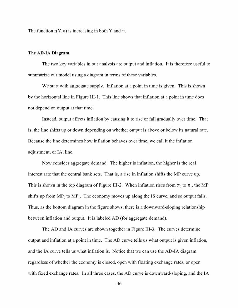
46

The function r(Y,B) is increasing in both Y and B.

The AD-IA Diagram

The two key variables in our analysis are output and inflation. It is therefore useful to

summarize our model using a diagram in terms of these variables.

We start with aggregate supply. Inflation at a point in time is given. This is shown

by the horizontal line in Figure III-1. This line shows that inflation at a point in time does

not depend on output at that time.

Instead, output affects inflation by causing it to rise or fall gradually over time. That

is, the line shifts up or down depending on whether output is above or below its natural rate.

Because the line determines how inflation behaves over time, we call it the inflation

adjustment, or IA, line.

Now consider aggregate demand. The higher is inflation, the higher is the real

interest rate that the central bank sets. That is, a rise in inflation shifts the MP curve up.

This is shown in the top diagram of Figure III-2. When inflation rises from B0 to B1, the MP

shifts up from MP0 to MP1. The economy moves up along the IS curve, and so output falls.

Thus, as the bottom diagram in the figure shows, there is a downward-sloping relationship

between inflation and output. It is labeled AD (for aggregate demand).

The AD and IA curves are shown together in Figure III-3. The curves determine

output and inflation at a point in time. The AD curve tells us what output is given inflation,

and the IA curve tells us what inflation is. Notice that we can use the AD-IA diagram

regardless of whether the economy is closed, open with floating exchange rates, or open

with fixed exchange rates. In all three cases, the AD curve is downward-sloping, and the IA

3 Throughout our analysis of the short run, we will neglect the fact that technologicalprogress and increases in the labor force and the capital stock cause the natural rate of outputto be rising over time. Thus we will keep the Y

_ line fixed rather than showing it as shifting

gradually to the right. Accounting for changes in Y_

makes the analysis more complicatedwithout giving us any important additional insights.

47

curve is horizontal and moves up or down depending on whether output is above or below its

natural rate.

The Behavior of Output and Inflation over Time

The final step in our analysis is to describe how inflation and output change. To

address this issue, we must bring in the rest of our assumption about aggregate supply:

although inflation at a point in time is given, it rises if output is above its natural rate and

falls if it is below. This is shown in Figure III-4, which adds a dashed vertical line at the

natural rate of output to the AD-IA diagram. Output is determined by the intersection of the

AD and IA curves (point A in the diagram). Thus to see if output is above or below its

natural rate, we need to look at whether this intersection is to the right or the left of the

Y = Y_

line. In the case shown, it is to the right; that is, output is above its natural rate.

According to our assumption about aggregate supply, this means that inflation is rising. This

is shown by the arrows above the IA line.3

As the IA line shifts up, inflation and output move along the AD curve. Thus

inflation is rising and output falling. This is shown by the arrows on the AD curve. In the

background, the increases in inflation are causing the central bank to raise the real interest

rate for a given level of output, and these changes in monetary policy are causing output to

fall. These shifts of the MP curve in response to changes in inflation in the IS-MP diagram

4 See Mankiw, Section 10-1.

48

correspond to movements along the AD curve in the AD-IA diagram.

Since output was initially greater than its natural rate, it remains above even after it

has fallen somewhat. Thus inflation continues to rise. The process continues until output

reaches its natural rate. This is the point labeled ELR (for long run) in the diagram. Once the

economy reaches that point, our assumption about inflation implies that inflation remains

steady. Thus, there is no further change in inflation or output until some type of disturbance

occurs.

Figure III-5 shows the long-run equilibrium. The IA curve comes to rest at the point

where it intersects the AD curve at Y = Y_

. Since output is at its natural rate, inflation is

steady -- that is, the IA curve is no longer shifting.

Finally, one can use the IS-MP diagram to see what the real interest rate is at the

long-run equilibrium. Output equals its natural rate. Thus the IS and MP curves must

intersect at Y = Y_

. This is shown in Figure III-6. As that diagram shows, the real interest

rate in a long-run equilibrium is the value of r on the IS curve at Y = Y_

. This is labeled rLR

in the diagram.

As one would expect, the level of the real interest rate in the long run implied by the

analysis is the same as the level we would find if we just assumed that prices are flexible,

and that output therefore equals its natural rate. Remember that another way of thinking

about the IS curve is that it shows, as a function of output, the real interest rate at which the

market for loans is in equilibrium.4 That is, if we are considering a closed economy, the IS

curve shows the real interest rate at which saving and investment are equal as a function of

5 Analyzing the long-run equilibrium of an open economy with fixed exchange rates isnot very interesting. If the economy's reserve loss in the long run is zero, this means thelong-run equilibrium is the same as it would be if the central bank were letting exchangerates float. And if the economy's long-run reserve loss is negative, this means that thecentral bank is accumulating reserves of foreign currencies indefinitely, which is notrealistic.

49

output. If we are considering an open economy with floating exchange rates, the curve

shows, as a function of output, the real interest rate at which saving equals the sum of

investment and net foreign investment. Thus, the long-run real interest rate shown in Figure

III-6 is simply the real interest rate that equilibrates the market for loans when output is at its

natural rate.5

III-2 Changes on the Aggregate Demand Side of the Economy

Now that we have developed our model, we can use it to understand how various

developments affect the economy. This section considers changes involving aggregate

demand. The next section considers changes involving aggregate supply.

Fiscal Policy

Our first example is the one we usually start with: an increase in government

purchases. Specifically, we consider a situation where the economy starts in a long-run

equilibrium. That is, output equals its natural rate, and as a result inflation is steady at some

level. There is then an increase in government purchases. Specifically, government

purchases rise from their initial level to a higher level, and then remain at that higher level.

50

Because this is our first example, we will work through it in detail.

We begin by considering the immediate effects of the increases -- that is, the effects

before inflation starts to change. To do this, we use the IS-MP model from Section I. The

increase in government purchases shifts the IS curve to the right. The result, as Figure III-7

shows, is that output and the interest rate both rise.

The IS-MP diagram shows that at the initial level of inflation, output is higher than

before. We could repeat this analysis for other inflation rates. Each time we considered a

different rate we would have to shift the MP curve, because inflation affects the real interest

rate the central bank sets for a given level of output. But each time, the increase in

government purchases would shift the IS curve to the right, and so output would be higher at

that inflation rate than before.

What this analysis is telling us is that the rise in government purchases shifts the AD

curved to the right: at a given inflation rate, output is higher than before. This is shown

together with the IA line in Figure III-8. The figure confirms what we already know from

the IS-MP diagram and the fact that inflation does not respond immediately to economic

developments: the immediate effect of the increase in government purchases is to raise

output and leave inflation unchanged.

The importance of the AD-IA diagram is that it allows us to trace out the effects of

the increase in government purchases after its immediate impact. Since government

purchases remain at their higher level, there are no additional shifts of the AD curve. But

output is now above its natural rate. Thus inflation rises; that is, the IA curve begins to shift

up. Output falls back toward the natural rate and inflation increases as the economy moves

up along the AD curve. This process is depicted in Figure III-9.

6 See Mankiw, Section 3-4.

51

The process continues until output returns to its natural rate; this is shown as point

E1LR in the figure. At that point, there are no further changes in inflation. Thus inflation is

steady at a higher level than it began. That is, the IA curve stops moving when it intersects

the new AD curve at Y = Y_

(point E1LR).

In the background, the increases in inflation are causing the central bank to raise the

real interest rate at a given level of output. That is, the MP curve is shifting up. The

economy moves up along the downward-sloping IS curve, so the real interest rate rises and

output falls. The process continues until output returns to its natural rate. Thus, the real

interest rate increases immediately because of the increase in government purchases, and

then rises gradually further as the economy is moving to its new long-run equilibrium

because inflation is rising.

Figure III-10 shows the positions of the IS and MP curves in the new long-run

equilibrium. The IS curve is to the right of where it was initially because of the increase in

government purchases. The MP curve is above where it was initially because of the rise in

inflation. Thus the diagram also shows us that the increase in government purchases raises

the real interest rate in the long run. This result is consistent with what you have already

learned about the long-run effects of an increase in government purchases.6

We can also see how the increase in government purchases affects the different

components of output. Consumption depends on disposable income, Y-T. Since the event

we are considering does not involve any changes in taxes, the behavior of consumption is

similar to the behavior of output. Consumption rises at the time of the increase in

52

government purchases because of the increase in output, and then declines gradually back to

its initial level as output returns to its natural rate.

Investment is determined by the real interest rate; the higher is the real interest rate,

the lower is investment. Thus investment falls at the time of the increase in government

purchases (because of the initial rise in the interest rate), and then falls more as the economy

adjusts to its new long-run equilibrium (because of the additional increases in the interest

rate).

The behavior of net exports depends on whether exchange rates are floating or fixed.

When they are floating, we find the behavior of net exports from the fact that they must

equal net foreign investment (see Section II-1). Net foreign investment is a decreasing

function of the real interest rate. Thus net foreign investment -- and hence net exports --

falls at the time of the increase in government purchases, and falls further as the economy

moves to its new long-run equilibrium. In the background, the exchange rate is adjusting so

that net exports equal the level of net foreign investment determined by the real interest rate

at each point in time. Thus the exchange rate appreciates at the time of the increase in

government purchases, and increases more after that. If we wanted to, we could show all of

this using a three-diagram figure like that in Figure II-3.

If exchange rates are fixed, on the other hand, net exports do not change in response

to the change in government purchases. Net exports depend on the real exchange rate:

NX = NX(g). With the exchange rate fixed at g_

, net exports do not change. Instead, the rise

in government purchases affects the central bank's reserve position. Recall that the reserve

loss equals the difference between private net foreign investment and net exports (see

Section II-3). Although net exports do not change, private net foreign investment does.

53

Specifically, it falls when government purchases rise (because of the rise in the real interest

rate), and falls more as the economy moves to its new long-run equilibrium (because of the

additional increases in the real interest rate). Thus the reserve loss becomes smaller. That

is, the increase in government purchases strengthens the central bank's reserve position.

Again, we could show this in detail using a diagram like Figure II-7 if we wanted to.

In practice, of course, the economy is never exactly in a long-run equilibrium when a

change occurs, and there are always other developments as the economy is adjusting to the

change. The reason for making the unrealistic assumption that the increase in government

purchases is the only force influencing the economy is that it allows us to see the effects of

the increase clearly. If the economy begins away from a long-run equilibrium or there are

other shocks while the economy is adjusting to the increase in government purchases, the

analysis we have done would show how an increase in purchases would cause the path of the

economy to differ from what it would have been otherwise. Suppose, for example, that the

rise in government purchases occurs when output is already above its natural rate. In the

absence of the increase, inflation would have risen gradually and output would have returned

gradually to its natural rate. In this case, the increase in government purchases causes output

to rise farther above its natural rate and to take longer to return to the natural rate than it

would have otherwise, and cause inflation to rise by more than it would have otherwise. To

avoiding cluttering up the discussion with endless references to what would have happened

otherwise, we focus on the case where the only development affecting the economy is the

increase in government purchases.

54

Monetary Policy

The government's other major tool for influencing the macroeconomy in the short run

is monetary policy. To see how monetary policy affects the economy, suppose there is a

shift to a tighter monetary policy rule. That is, suppose the central bank changes its rule so

that at a given level of output and inflation, it sets a higher real interest rate than before. Its

reason for doing this might be to reduce inflation. Again, to see the effects of this

development clearly, we assume that the economy is initially in a long-run equilibrium and

that there are no additional disturbances while the economy is moving to its new long-run

equilibrium.

As before, we use the IS-MP diagram to find the immediate effects of the change. At

the initial inflation rate, the central bank is setting a higher interest rate at a given level of

output than before. Thus the MP curve shifts up. The interest rate rises and output falls.

This is shown in Figure III-11.

This analysis tells us that at a given level of inflation, output is lower than before.

That is, the AD curve shifts to the left. Since output started at its natural rate, it is now

below. Thus inflation starts to fall; that is, the IA line begins to shift down. Since the

central bank makes no additional changes in its rule for setting the interest rate, the AD

curve does not shift again. The economy moves down along the new AD curve, with output

rising back towards its natural rate. As long as output is below Y_

, inflation continues to fall.

All of this is shown in Figure III-12. The economy comes to rest at point E1LR. Once it is

there, inflation is steady at a lower level than it began. Thus the central bank has succeeded

in reducing inflation -- though at the cost of putting the economy through a period when

output is below its natural rate.

7 See Mankiw, Chapter 4.

55

We can again use IS-MP analysis to find the long-run effect of the change on the

interest rate. The change in the monetary policy rule corresponded to an upward shift of the

MP curve. This is shown as the move from MP0 to MP1 in Figure III-13. This change

produced the shift of the AD curve. Then as inflation fell, the MP curve shifted down.

These changes corresponded to the movements along the AD curve: the reason the AD curve

slopes down is that when inflation is lower, the central bank sets a lower real interest rate at

a given level of output. Throughout the process, there is no change in the IS curve. Thus

when Y returns to Y_

, the MP curve must be back in its original position. This is shown by

the fact that MPLR is in the same place as MP0 in the diagram. It follows that in the new

long-run equilibrium, the real interest rate is the same as it was before the change in policy.

Notice that the change in monetary policy does not affect any real variables in the

long run. Output and the real interest rate both return to their initial values; only inflation

changes permanently. This is consistent with what you have already learned: in the long

run, monetary changes do not affect real variables (like output), only nominal ones (like

inflation).7

There have been many actual episodes like this one. In the United States, the clearest

example is the "Volcker disinflation" of the early 1980s. In October 1979, under the

leadership of Paul Volcker, the Federal Reserve made a major shift to tighter monetary

policy because it believed that inflation was much too high. The result was a period of very

high interest rates, below-normal output, and high unemployment. The unemployment rate

peaked at 10.8 percent at the end of 1982. Inflation fell rapidly. As it fell, the Federal

56

Reserve reduced the real interest rate. By 1986, output and unemployment had returned to

roughly their natural rates, and inflation had fallen from almost 10 percent to below 4

percent.

Monetary Policy and Inflation in the Long Run

This analysis shows that monetary policy is a critical determinant of inflation in the

long run. Suppose the central bank follows a fairly loose monetary policy rule -- that is, a

rule that sets a relatively low real interest rate when inflation is low or moderate unless

output is well above its natural rate. With such a rule, monetary policy tends to push output

above the natural rate when inflation is low or moderate. The result is that inflation rises,

and thus that it is high in the long run. If the central bank follows a fairly tight policy rule,

on the other hand, inflation is low in the long run.

We can be more specific about the relation between the central bank's rule and

inflation in the long run. Monetary policy does not affect either output or the real interest

rate in the long run. Output equals its natural rate, and the real interest rate equals the value

that brings the loan market into equilibrium when output is at that level. The inflation rate in

the long run is therefore the inflation rate that causes the central bank to set the real interest

rate to the level that equilibrates the loan market when output equals its natural rate. In other

words, the inflation rate in the long run is the rate that causes the MP curve to cross the IS

curve at Y = Y_

.

An example may clarify this point. Suppose the central bank's rule for the real

interest rate is linear. Specifically, suppose the function r = r(Y,B) takes the form

57

r = a + bB + c[Y - Y_

].

Here b is a parameter showing how the central bank responds to inflation: if inflation rises

by a percentage point, the central bank raises the real interest rate by b percentage points.

Similarly, c shows how it responds to departures of output from normal. If Y - Y_

rises by

one unit, the central bank raises r by c percentage points. Both b and c are positive. Finally,

a is the intercept term of this linear rule. It shows what real interest rate the central bank

would set if inflation were zero and output equaled its natural rate.

Let rLR denote the value of the real interest rate given by the IS curve when output

equals its natural rate. We know that in the long run, Y = Y_

and r = rLR. Thus if the central

bank follows the rule given above, inflation in the long run, which we will call BLR, is the

solution to the equation

rLR = a + bBLR + c[0].

Solving this equation for BLR gives us

rLR - a BLR = . b

A higher value of a -- which corresponds to a rule that sets a higher real interest rate at a

given level of inflation and output -- produces lower inflation in the long run. Likewise,

suppose that rLR - a is positive; this is what is needed for inflation to be positive in the long

8 Of course this is not done by mechanically following a rule like those we havediscussed. Instead the central bank adjusts the interest rate in response to economicdevelopments in a way that is intended to keep inflation close to the long-run goal. Oneconsequence is that policy is well described by a rule of the sort we have been discussing.

9 This analysis shows that the central bank's real interest rate rule is a crucial determinantof inflation in the long run. You learned earlier that the growth rate of the money stock is acrucial determinant of inflation in the long run (see Mankiw, Chapter 4). The way these twoconclusions are related involves how the central bank controls the real interest rate. Recallfrom Section I-3 that it does this by adjusting the money supply. Thus in setting the real

58

run. Then a rule that responds more to increases in inflation (that is, that has a higher b)

produces lower inflation in the long run. Finally, because output equals its natural rate in the

long run, inflation is not affected in the long run by how the central bank responds to

departures of output from its natural rate (that is, it is not affected by the parameter c).

Because of monetary policy's crucial role in determining inflation in the long run,

most central banks today design their policies with a focus on their implications for inflation.

In some countries, such as the United Kingdom and Canada, this is done through formal

inflation targeting. The central bank begins by choosing a long-run goal for inflation. It then

adjusts the real interest rate in response to output and inflation with that goal in mind.8

Because many different interest rate polices produce the same level of inflation in the long

run, inflation targeting takes many forms. The central bank can change the real interest rate

more or less aggressively in response to departures of inflation from the target, and more or

less aggressively in response to departures of output from its natural rate. In terms of our

example of a linear rule, the level of inflation in the long run, BLR, does not dictate the exact

values the parameters b and c must take. But by conducting policy with a focus on the level

of inflation in the long run, over the last decade central banks in many countries have

succeeded in bringing inflation down to low levels and keeping it there.9

interest rate, in the background it is choosing the money growth rate. Since the condition forequilibrium in the money market -- M/P = L(i,Y) � is the same here as in your earlieranalysis of inflation in the long run, the same long-run relationship between money growthand inflation holds here as in your earlier analysis. For example, suppose the central bank isfollowing a real interest rate rule that produces low inflation in the long run. To carry outsuch a rule, the central bank needs to keep money growth low. When inflation is low andoutput equals its natural rate, for example, high money growth would raise the supply of realmoney balances, and thus lower the real interest rate; this in turn would raise output abovenormal and hence cause inflation to start to rise. As in Section I-3, the details of how thecentral bank adjusts the money supply to carry out its rule are not important. The importantpoint is simply that the earlier conclusions about money growth and inflation in the long runcontinue to hold.

59

III-3 Changes on the Aggregate Supply Side of the Economy

Inflation Shocks and Supply Shocks

We now turn to the effects of changes in aggregate supply. There are two main types

of changes: inflation shocks and supply shocks. Since the distinction between them is

important, the first step is to define them:

An inflation shock is a disturbance to the usual behavior of inflation that shifts the

inflation adjustment line. A supply shock is a change in the natural rate of output.

Let us consider each of these in turn. An inflation shock occurs when some

development causes firms to set their prices in a way that differs from the usual pattern.

Recall that normally the rate at which firms raise their prices -- that is, the inflation rate --

rises when output is above its natural rate and falls when output is below its natural rate. An

unfavorable inflation shock is an event that causes inflation to jump to a higher level; a

60

favorable inflation shock is an event that causes it to jump to a lower level. The classic

example of an inflation shock is an oil shock -- a sudden change in oil prices. In the winter

of 1973-1974 and again in 1979, the Organization of Petroleum Exporting Countries (OPEC)

raised the price of oil dramatically. Since oil prices are a component of firms' costs, these

increases caused firms to raise the prices of their products by more than before. That is, they

caused inflation to jump to a higher level. In terms of our model, they caused an upward

shift of the IA line. And these increases in inflation had nothing to do with the level of

output; they were a result of the increases in oil prices.

To think about inflation shocks more systematically, it is helpful to list the

ingredients that go into firms' choices of their prices:

" The first ingredient is the wages that firms pay. All else equal, the

higher are wages, the higher are firms' costs, and thus the higher are the prices

they charge.

" The second ingredient is labor costs other than wages. Employing

workers involves not just the wages they are paid, but payroll taxes, fringe

benefits like health insurance, and so on.

" The third ingredient is the costs of inputs other than labor, such as

oil, other raw materials, and goods purchased from other firms.

" The fourth ingredient is productivity. When firms can produce more

using a given amount of labor and a given quantity of other inputs, their costs

are lower, and so (all else equal) their prices are lower.

" The final ingredient is the relationship between prices and costs. In

61

a perfectly competitive market, firms set their prices equal to their marginal

costs. But actual markets are not perfectly competitive; prices usually exceed

marginal costs. The greater is this gap, the higher are prices (again, all else

equal).

This list of ingredients allows us to see what kinds of developments cause inflation

shocks. An inflation shock can arise from any of these ingredients. For example, wages

might rise unusually fast because of a change in labor laws that increases unions' bargaining

power; this would cause an unfavorable inflation shock stemming from the first ingredient of

firms' pricing decisions. Rises in the cost of health insurance are an important example of

unfavorable inflation shocks involving the costs of hiring labor other than wages. Increases

in oil prices are a type of unfavorable inflation shock involving the costs of inputs other than

labor. And declines in productivity (which lead to higher costs) and increases in monopoly

power (which increase the gap between prices and costs) are also potential sources of

unfavorable inflation shocks.

Of course, inflation shocks can be favorable as well. In the United States, inflation

has not risen over the past few years despite the fact that output is almost certainly well

above its natural rate. The reason is that there have been a series of favorable inflation

shocks. The prices of oil and other raw materials have plummeted. Rises in health

insurance costs have been less than the overall inflation rate. And increased competition

from foreign firms appears to have reduced the average gap between firms' prices and their

marginal costs.

It is also important to remember that not all changes in inflation are inflation shocks.

62

If firms raise wages, and thus prices, more than before because unemployment is very low,

this is the usual response of inflation to above-normal output, not an inflation shock. The

same is true if firms find that their costs are high because they are operating close to

maximum capacity.

Supply shocks are easier to describe that inflation shocks. A supply shock is a

change in the natural rate of output, Y_

. There are two sources of supply shocks. The first is

changes in the inputs that would be available if the economy were operating at its natural

rate. Two examples of this type of supply shock are a change in the labor force and a

change in the natural rate of unemployment. Both of these changes affect the number of

workers when the economy is operating at its normal level, and thus affect Y_

. The second

source of supply shocks is changes in output for a given level of inputs -- that is, a change in

productivity. Notice that this means that a change in productivity leads to both an inflation

shock and a supply shock. That is, it both shifts the inflation adjustment line and alters the

natural rate of output.

The Effects of an Inflation Shock

Now that we have described possible sources of disturbances on the supply side of

the economy, we can analyze their effects. We begin with an unfavorable inflation shock.

For concreteness, suppose that initially the economy is in a long-run equilibrium, and that

there is a sudden rise in oil prices.

The immediate effects of this change are shown in Figure III-14. The inflation shock

shifts the inflation adjustment line up. In terms of the figure, at the time of the shock the IA

line shifts from IA0 to IA1. The economy moves up along the aggregate demand curve.

63

Output falls and inflation rises -- a combination that was dubbed "stagflation" in the 1970s.

In the background, the central bank is raising the real interest rate in response to the rise in

inflation.

Changes in oil prices have little impact on the economy's natural rate of output. Thus

output is now below its natural rate. And since the event we are considering is a one-time

rise in oil prices, there are no further inflation shocks. Thus inflation begins to fall; that is,

as Figure III-15 shows, the IA line begins to move down. Inflation falls and output rises.

The process continues until output returns to its natural rate. When it does, inflation is back

at its initial level. Thus, the unfavorable inflation shock causes a period of high inflation and

below-normal output.

The Effects of a Supply Shock

Our second example is a fall in the natural rate of unemployment, u-. With a lower

natural rate of unemployment, the economy's normal level of employment is higher, and so

its natural rate of output is higher. Again, we assume that the economy begins in a long-run

equilibrium.

The immediate effect of this development is a little surprising: neither output nor

inflation change. In the absence of an inflation shock, inflation at a point in time is given.

Thus inflation does not change immediately. And since neither the IS nor the MP curve is

affected by the change, output does not change either.

Nonetheless, the fall in the natural rate of unemployment does matter. Because the

natural rate of output is higher than before and actual output is unchanged, output is now

below its natural rate. Thus inflation begins to fall. As it falls, output rises. This continues

64

until output equals its new natural rate. At that point, inflation is steady at a lower level than

it began, and there are no further changes in output. Figure III-16 summarizes this analysis.

It shows the gradual downward shift of the IA line and the economy's movement down along

the AD curve from its initial position (point E0LR) to the new long-run equilibrium (point E1

LR).

A fall in the natural rate of unemployment appears to be another reason for the U.S.

economy's excellent performance over the past few years. In the early 1990s, the natural

rate of unemployment appears to have been slightly over six percent. But various

developments, including changes in the demographic composition of the labor force, appear

to have reduced it to between five and six percent today. This decline in the natural rate has

been accompanied by rising output and falling inflation, just as our model predicts.

Inflation Expectations and Inflation Shocks

Our final topic in this section is a source of inflation shocks that is somewhat

different from the others we have considered. Think about a firm deciding what wage to pay

for the coming year. One factor it will consider is that amount of inflation it expects during

the year. If, for example, it expects a great deal of inflation, it will want to set a fairly high

wage to make sure that it is paying an adequate amount at the end of year. And when the

firm sets a higher wage, it will charge a higher price for its product. The same analysis

applies to a firm and a union bargaining over what wage the firm will pay over the next few

years, or to a firm deciding what price to charge for its product for the next year: the higher

is expected inflation, the higher are the wages and prices that are set now. What this

analysis is telling us is that changes in expected inflation cause inflation shocks. They cause

a change in the behavior of prices that is not simply a response to whether output is above or

65

below its natural rate.

One important implication of this discussion is that the credibility of a policy to

reduce inflation can have important effects on the costs of getting inflation down. Consider

first a central bank with a poor record of fighting inflation and of carrying out its announced

policies. Suppose this central bank announces that it is changing its policy rule to set a

higher interest rate at a given level of output and inflation than it did before in order to bring

inflation down. Given the bank's track record, firms and workers are not likely to expect it

to stick with the new policy for long. Thus their expectations of inflation change little. If

the bank then carries through with its plan, the resulting shift of the AD curve leads to a fall

in output. The central bank succeeds in reducing inflation, but only at the cost of a

recession. That is, the analysis we did in Section III-2 applies.

Now consider a central bank with a strong record of fighting inflation and of sticking

with its announced policies. When this central bank announces a shift to a tighter rule,

expected inflation is likely to fall. Thus the announcement of the policy change generates a

favorable inflation shock. This development is analyzed in Figure III-17. The bank's policy

shift causes a leftward shift of the AD curve, as before; this is shown as the shift from AD0

to AD1. But the favorable inflation shock shifts the IA curve; this is shown as the shift from

IA0 to IA1. The result is an immediate fall in inflation and a smaller fall in output. In terms

of the diagram, the immediate effect of the change is to move the economy from point E0LR to

point A. In contrast, without credibility there is no immediate effect on inflation, and so the

economy moves to point B. After the initial move, the economy moves down the new AD

curve to the new long-run equilibrium (point E1LR). Thus credibility reduces the cost of

getting inflation down.

10 For some evidence on the merits of the two positions, see Thomas J. Sargent, "TheEnds of Four Big Inflations," in Robert E. Hall, ed., Inflation (Chicago: University ofChicago Press, 1982), pp. 41-98; and Guy Debelle, "The Ends of Three Small Inflations: Australia, New Zealand, and Canada," Canadian Public Policy 22 (March 1996), pp. 56-78.

66

The importance of changes in expected inflation in causing inflation shocks is

controversial. As a result, there is disagreement about how important credibility is to the

costs of reducing inflation. One view is that expected inflation is a crucial determinant of

the behavior of actual inflation. In this case, a fully credible policy can reduce inflation at

almost no cost in terms of lost output: when a credible central bank announces its plan to

bring inflation down, actual inflation drops almost immediately to the level it will attain in

the new long-run equilibrium. The opposing view is that firms and workers rely mainly on

past inflation and the current state of the economy in setting prices and wages. In this view,

even a very credible policy change has little immediate impact on how prices and wages are

set, and so our usual assumption that inflation falls only when output is below normal is still

a good first approximation.10

67

PROBLEMS

1. Describe how, if at all, each of the following developments affects the AD and/orIA curves:

a. Individuals become more optimistic about their future incomes, and thereforeconsume more out of a given amount of disposable income than before.

b. Exchange rates are fixed, and American goods become more fashionable -- that is,foreign demand for American goods at a given real exchange rate increases.

c. Exchange rates are floating, and American goods become more fashionable.d. Anti-trust laws are relaxed, so firms charge higher prices for a given level of costs.e. The demand for money increases (that is, consumers' preferences change so that at

a given level of i and Y they want to hold more real balances than before).f. Investment demand becomes less sensitive to changes in the interest rate.g. Oil prices increase, and at the same time consumption for a given level of

disposable income falls.

2. Suppose that output is initially at its natural rate, and that there is a tax cut. Describe how output, inflation, the real interest rate, consumption, and investment respondto the tax cut, both immediately and over time.

3. Consider the shift to a tighter monetary policy rule analyzed in Section III-2. What are the immediate effects of the shift on consumption and investment? How doconsumption and investment behave as the economy is moving to its new long-runequilibrium?

4. Again consider the shift to a tighter monetary policy rule analyzed in Section III-2.a. If exchange rates are floating:

i. What is the immediate effect of the shift to a tighter monetary policy ruleon net exports and the exchange rate?

ii. How do net exports and the exchange rate behave as the economy ismoving toward its new long-run equilibrium?

b. If exchange rates are fixed:i. What is the immediate effect of the shift to a tighter monetary policy rule

on the reserve loss?ii. What is the behavior of the reserve loss as the economy is moving toward

its new long-run equilibrium?

5. Suppose that there is a technological disaster that makes workers less productivethan before. Assume that initially output is at its natural rate.

a. How, if at all, does this affect the IA curve?b. How, if at all, does this affect Y

_?

c. In light of your answers to (a) and (b), what is the immediate effect of the disasteron output and the real interest rate?

d. Can you tell how the long-run effect of the disaster on output compares with the

68

short-run effect? Explain.

6. Suppose the Federal Reserve, instead of following the rule r = r(Y,B), has a targetlevel of inflation. Specifically, it sets r according to r = rLR + b[B - B*], where rLR is the realinterest rate when the economy is in long-run equilibrium, b is some positive number, andB* is the target level of inflation. This rule states that the Federal Reserve raises the realinterest rate above its long-run level when inflation is above its target and lowers it below itslong-run level when inflation is below its target. Note that this rule means that if somedevelopment changes what the real interest rate will be in the long run, the Federal Reservechanges the real interest rate immediately.

a. With this monetary policy rule, is the MP curve upward-sloping, flat, ordownward-sloping? Explain.

b. Is the AD curve upward-sloping, flat, or downward-sloping? Explain.c. Assume the economy starts in a situation where B = B* (so r = rLR) and Y = Y

_.

Thus the economy is in a long-run equilibrium. Describe the immediate effects of each ofthe following developments on output, inflation, and the real interest rate:

i. Government purchases rise.ii. There is an unfavorable inflation shock.

iii. The Federal Reserve reduces its inflation target, B*.

7. Suppose that initially output equals its natural rate, and that inflation is thereforesteady. Now suppose that there is a sudden loss of investor confidence in a country, so thatthere is a large increase in net foreign investment at a given real interest rate. Further,suppose that, in addition to our usual assumptions, the real exchange rate matters foraggregate supply. Specifically, suppose that a rise in the real exchange rate (because itlowers the costs of firms that import some of their inputs) is a favorable inflation shock, andthat a fall is an unfavorable shock. Finally, assume that exchange rates are floating.

a. How, if at all, does the loss of confidence affect the AD curve?b. How, if at all, does the loss of confidence affect the IA line?

8. Do you agree or disagree with each of the following statements? Defend youranswers.

a. "In the absence of inflation shocks, times of falling output cannot be times offalling inflation."

b. "In the absence of inflation shocks, times when output is below its natural ratecannot be times of falling inflation."