Short- and long-term demand curves for stocks: Evidence on the dynamics of

arbitrage

Robin Greenwood* rgreenwood@hbs.edu

First draft: October 2000 This draft: March 17, 2003

Abstract I derive a simple model of demand curves for portfolios of assets at different time horizons and apply it to a unique index rebalancing event in Japan. In the short-run, demand curves are downward sloping, with the slope determined by the contribution of the portfolio of assets to the total risk of a diversified arbitrageur. Demand curves flatten over time, reducing the long-term effects of changes in the supply of assets on prices. The model is applied to a redefinition of the Nikkei 225 stock index, in which 30 stocks were replaced and 195 stocks were significantly downweighted. The event caused an estimated ¥2 trillion in rebalancing by institutional investors. During a week with no major economic news, the additions gained 19%, the deletions fell by 32%, and the remainders fell by 13%. More than 70% of these returns were reversed within 20 weeks of the event. Consistent with the model, stocks with lower (higher) event returns experienced higher (lower) post-event returns.

* Harvard Business School. A previous version of this paper was circulated under the title “Large Events and Limited Arbitrage: Evidence from a Japanese stock Index Redefinition”. I thank Malcolm Baker, Ken Froot, Seki Obata, Jorge Rodriguez, Mark Seasholes, Josh White, Andrei Shleifer, Nathan Sosner, Jeremy Stein, Jeffrey Wurgler and seminar participants at MIT and Harvard for helpful comments.

Short- and long-term demand curves for stocks: Evidence on the dynamics of

arbitrage

Abstract I derive a simple model of demand curves for portfolios of assets at different time horizons and apply it to a unique index rebalancing event in Japan. In the short-run, demand curves are downward sloping, with the slope determined by the contribution of the portfolio of assets to the total risk of a diversified arbitrageur. Demand curves flatten over time, reducing the long-term effects of changes in the supply of assets on prices. The model is applied to a redefinition of the Nikkei 225 stock index, in which 30 stocks were replaced and 195 stocks were significantly downweighted. The event caused an estimated ¥2 trillion in rebalancing by institutional investors. During a week with no major economic news, the additions gained 19%, the deletions fell by 32%, and the remainders fell by 13%. More than 70% of these returns were reversed within 20 weeks of the event. Consistent with the model, stocks with lower (higher) event returns experienced higher (lower) post-event returns.

1. Introduction

In traditional finance theory, asset prices respond only to changes in expected cash flows

and discount factors. Uninformed changes in investor demand have no effect on prices, even in

the short-run. According to the theory, if securities have perfect substitutes, then investors will

always be willing to buy when the price of an asset falls slightly under the fundamental value, or

sell when the price rises slightly above. Arbitrage thus keeps the demand curve flat.

While theoretically compelling, perfect arbitrage cannot explain numerous examples in

which uninformed investor demand for securities does affect prices, at least in the short-run.

Shleifer (1986), Harris and Gurel (1986), and Wurgler and Zhurvaskaya (2002) and others find

that the price of a stock rises when it is added to a stock index, or when its weight in the index

rises (Kaul, Mehrotra and Morck (2000)).1 These papers argue that the increase in price cannot

be attributed to new information about these firms, but rather to institutional investor demand for

the stock. In short, the demand curve for stocks is downward sloping. Recent research ties

downward sloping demand curves to a wide range of phenomena in capital markets, such as

excess volatility (Harris (1989), excess comovement of returns (e.g. Hardouvelis, La Porta,

Wizman (1994), Pindyck and Rotemberg (1993), Froot and Dabora (1998), Barberis, Wurgler

and Shleifer (2002)), or discrepancies in the relative prices of asset classes (Barberis and Shleifer

(2002)).

Although there may no longer be much debate that demand curves for stock are

downward sloping in the short run, little is known about demand curves in the long run. It

seems reasonable that demand shocks have larger short-run effects on prices because of

1 See also Dhillon and Johnson (1991), Goetzmann and Garry (1986), Lynch and Mendenhall (1997) and Liu (2000).

3

temporary imbalances between demand and supply—a phenomenon often called “price

pressure.” But this imbalance is by definition only temporary, with the implication that the

demand curve must flatten over time.2 Nevertheless, researchers have found it difficult to

identify this flattening in the data. Shleifer (1986) finds that prices do not revert following

inclusion into the S&P index, while Lynch and Mendenhall (1997) document that initial event

returns are partially reversed after the event. Other research supports both conclusions. In any

case, since event returns following demand shocks are modest in comparison with the standard

deviation of returns at long horizons, most research focuses on identifying whether returns revert

at all, rather than by how much or at what speed. Even less is known about long-run effects of

demand when shocks simultaneously affect more than one asset.

This paper presents a simple limited arbitrage model of demand curves for stock at

different horizons. The model allows me to study the path of asset prices following multiple

demand shocks. Consistent with previous empirical evidence, the model predicts increases in

asset prices following decreases in the supply of the asset (net of exogenous demand), with the

amount of increase proportional to the marginal contribution of the demand shock to the risk of a

fully diversified portfolio. Following conventional CAPM logic, when more than one asset

experience shocks, the demand curve for the portfolio of assets may be flatter than demand

curves for individual assets. The model differs from other models of limited arbitrage, however,

in its characterization of medium- and long-run returns following changes in supply. I show that

after net purchases of a stock by index traders, prices rise initially but revert linearly over time,

with the speed of reversion proportional to the initial event return, itself proportional to the

2 This does not apply, however, to the cross-section. Wurgler and Zhurvaskaya (2002) find that arbitrage flattens the demand curve for stocks.

4

marginal contribution of the demand shock to the risk of the arbitrage portfolio.3 The reversion

in returns occurs because the ratio of arbitrage risk to fundamental risk falls over time. The

model yields the cross-sectional prediction that the speed of reversion should be proportional to

the initial event return.

I apply the model to a unique event in which 255 securities were subjected to

simultaneous uninformed demand shocks, which exceeded by far the typical daily trading

volume in those securities. The event is the April 2000 redefinition of the Nikkei 225 index in

Japan. As a result of the redefinition, thirty high-tech stocks replaced thirty smaller index

constituents, causing the weights of the remaining 195 securities to fall by nearly half, as the new

stocks represented a larger proportion of the index than those that had been dropped.4

Institutional investors tracking the Nikkei 225 index rebalanced their portfolios, buying additions

and selling deletions and about half of their holdings of the 195 remainders. Total trading linked

to the redefinition was about ¥2,000bn (approximately US$19bn). During the event week,

average turnover of each of the 255 stocks more than tripled.5 The additions gained 19%, the

deleted stocks fell by 32% and the remaining 195 stocks fell by an average of 13%. The rest of

the market was nearly flat – the value weighted TOPIX index dropped only 1.18% during the

week. Together, the 255 stocks affected by the event represented most of the equity market

capitalization in Japan.

The event has several features that make it suitable for testing the model, and for

understanding medium- and long-run demand curves for stock more generally. First, the 3 I use the notation “net purchases” and positive demand shock interchangeably. 4 This is partly due to an unusual weighting convention of the Nikkei index in which the index value is proportional to the sum of the ex-rights prices of its members, giving some stocks disproportionately high index representation. See Section 3 5 Average turnover (share volume / total shares) was 3.17 times the historical average, calculated using one-year of past turnover data.

5

redefinition involved a large number of securities, giving my study enough power to identify the

model using cross-sectional variation in event and post-event returns alone. Moreover, the

unusual weighting system of the Nikkei 225 yields additional variation in the size of the demand

shocks affecting individual stocks. For example, I make use of the fact that the risk incurred by

arbitrageurs accommodating demand for additions is hedged by their opposite positions in the

deletions and remainders. Second, the demand shocks are simultaneous, allowing me to hold

other factors constant with respect to the cross-section. Third, stocks displayed significant cross-

sectional variation in post-event returns, and more interestingly, most of the initial event returns

were reversed within 20 weeks of the event. Fourth, the event resulted in so much trading as to

surely test the risk capacity of professional arbitrageurs. This helps justify the assumption that

the preferences of diversified arbitrageurs determined the path of event and post-event prices.

Finally, to the extent that index changes may reflect new information about the prospective cash

flows of these firms, this concern is mitigated by 195 stocks that remained in the index yet still

experienced reductions in index weight. These stocks serve as a useful robustness check for

results obtained on the whole sample.

The model describes the short- and long-run path of prices as a function of the demand

shock, the fundamental risk of the securities, and the constraints on the arbitrage strategy. Event

returns (post-event returns) for each stock are (negatively) proportional to the marginal

contribution of the demand shock to the risk of a fully diversified portfolio. I also predict a

negative linear relationship between event returns and post-event returns. I confirm these

propositions and study the reversion of returns as a function of horizon. This reveals the long-

run profitability of arbitrage strategies during the event. Over 20% of the returns are reversed in

the week after the event, with at least 50% more reversed during the next 20 weeks. Although

the reversion of returns after the event is consistent with rewards to arbitrage, it is clear that any

6

arbitrage strategy did involve considerable risk. For example, an arbitrageur who accommodated

only 1% of the total demand shock on April 14 would have lost ¥4.17 billion (over US$ 39

million) by the end of the following week and would have only recouped this loss by

November.6 Even a strategy that sold when prices were at their peak would have experienced a

loss of over ¥0.3 billion in one of the post-event weeks.

The paper proceeds as follows. Section 2 outlines a model of multi-security arbitrage.

Section 3 describes the Nikkei 225 index redefinition and presents the details of index

construction and portfolio rebalancing. Section 4 presents the basic tests of the model. Section 5

looks at the profitability of different arbitrage strategies. Section 6 concludes.

2. Arbitrage with many stocks

A simple limits-to-arbitrage model describes the effects of multiple demand shocks on

asset returns. On day t*, all securities receive an unexpected demand shock, changing the net

supply of assets thereafter. Arbitrageurs accommodate the demand shock but receive higher

expected returns in compensation for their increased risk bearing. Expected total returns decline

over time, reversing the returns incurred because of the demand shock. The framework can be

readily applied to understand the effects of the event returns (the vector of returns between t*-1

and t*) and the reversion of returns (returns between t* and t*+k). When demand shocks include

more than one security, the demand curve for one stock does not exist independently of the

demand curve for the others.

To analyze both event returns and the slow reversion of stock returns after a change in net

supply requires a model with many periods. I rely on a theoretical framework developed in

6 This is based on April 14 prices. See Figure 3.

7

Hong and Stein (1999) and Barberis and Shleifer (2002). Most of the derivations are left for the

appendix, while the main results are presented in the text.

A. Setup

The capital market includes N risky securities in fixed supply with supply vector given by

Q. There is a risk-free asset in perfectly elastic supply with net return normalized to zero. Each

security pays a liquidating dividend at some time T. The information flow regarding dividend

TiD , is given by

∑=

+=t

ssiiti DD

1,0,, ε , for all i (1)

The information shocks si ,ε are identically and independently distributed over time and normal

with zero mean and covariance matrix Σ .

There are two types of agents operating in the capital market. Index traders own an

exogenous and fixed quantity of securities, denoted by the Nx1 vector u. For now, I normalize

this vector to zero. The other agents in the model are myopic mean-variance arbitrageurs. They

maximize exponential utility of next period wealth subject to a wealth constraint:

( )[ ]1expmax +−− ttNWE γ (2)

s.t. [ ]ttttt PPNWW −′+= ++ 11

tW , tP , and tN are arbitrageurs’ wealth, the vector of security prices, and arbitrageur demand at

period t, respectively.

I solve for the path of prices after a permanent shock to index trader demand u under two

different assumptions about arbitrageurs. In the first case, arbitrageurs are unconstrained. They

form an efficient portfolio that accommodates the entire demand shock. In the second case,

8

specialized arbitrageurs are constrained to invest in only one asset, but different amounts of these

traders may exist for each asset. Both cases have straightforward implications for event returns

and the reversion of event returns.

B. Solution for unconstrained arbitrageurs

The unconstrained solution to (2) is given by the (Nx1) demand vector

( )tttttT PPEPVarN −= +−

+ )()]([11

11γ

(3)

Consider the effects of a permanent demand shock. At *tt = , index trader holdings increase

from 0 to u . Denote positive elements of the vector u as “positive demand shocks” – they are

easily thought of as reductions in the net supply of assets. In equilibrium, total demand is equal

to total supply

uQNt −= (4)

Substituting in the demand function of arbitrageurs and rearranging gives

( ) ( )[ ]uQPVarPEP ttttt −−= ++ 11 γ (5)

In forming their demands, arbitrageurs are fully rational. This means that the conditional

variance of next period’s prices is equal to the actual variance of next period’s prices. This leads

to the first proposition.

Proposition 1 The vector of price changes for securities 1..N is given by

))(( *1 *** QutTPP ttt +−Σ+=−−

γε (6)

The expected reversion of prices between the event period *t and the period k periods after the

event is given by

9

( ) )(*** uQkPPEtktt

−Σ=−+

γ (7)

The covariance matrix of event price changes with reversion of prices is given by the negative

definite matrix

Σ⋅⋅Σ−−=∆∆+

)'()(),cov( 2*, *** uuEktTPP kttt γ (8)

The diagonal terms of this matrix are all negative. Proof: See appendix.

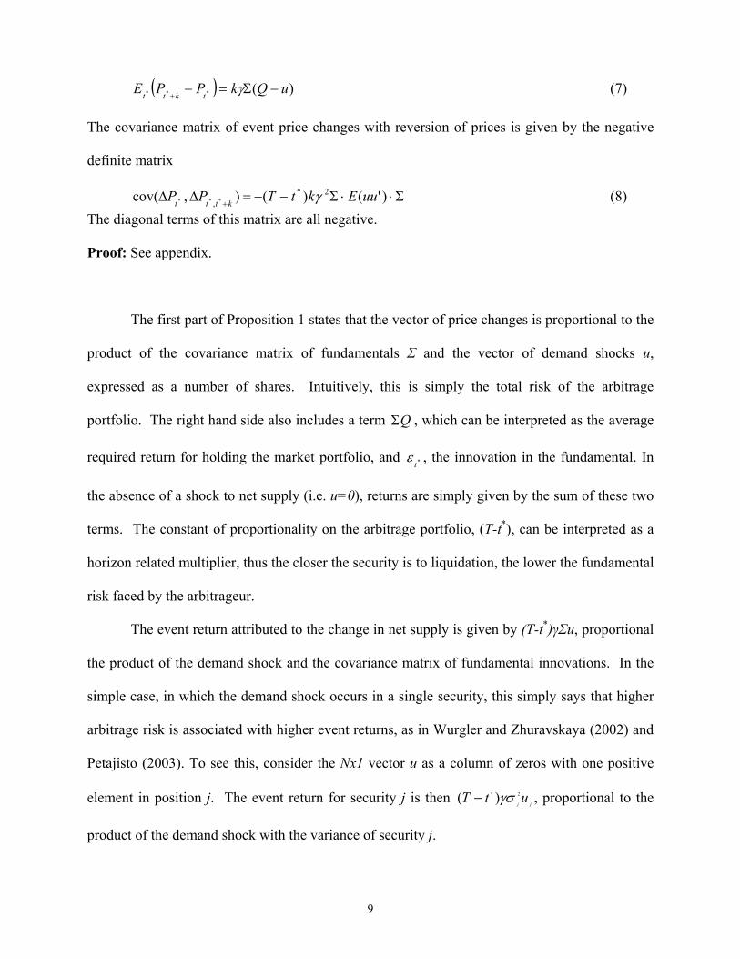
The first part of Proposition 1 states that the vector of price changes is proportional to the

product of the covariance matrix of fundamentals Σ and the vector of demand shocks u,

expressed as a number of shares. Intuitively, this is simply the total risk of the arbitrage

portfolio. The right hand side also includes a term QΣ , which can be interpreted as the average

required return for holding the market portfolio, and *tε , the innovation in the fundamental. In

the absence of a shock to net supply (i.e. u=0), returns are simply given by the sum of these two

terms. The constant of proportionality on the arbitrage portfolio, (T-t*), can be interpreted as a

horizon related multiplier, thus the closer the security is to liquidation, the lower the fundamental

risk faced by the arbitrageur.

The event return attributed to the change in net supply is given by (T-t*)γΣu, proportional

the product of the demand shock and the covariance matrix of fundamental innovations. In the

simple case, in which the demand shock occurs in a single security, this simply says that higher

arbitrage risk is associated with higher event returns, as in Wurgler and Zhuravskaya (2002) and

Petajisto (2003). To see this, consider the Nx1 vector u as a column of zeros with one positive

element in position j. The event return for security j is then jj

utT 2* )( γσ− , proportional to the

product of the demand shock with the variance of security j.

10

The model provides more insight, however, in the analysis of simultaneous demand

shocks to different securities. Consider again the Nx1 vector u, except with a positive element ui

(corresponding to an index addition, e.g.) in position i and negative element –uj (corresponding

to a deletion, e.g.) in position j. Event returns are )()( 2*

jjiijiiuutT σσρσγ −− for security i and

)()( 2*

ijiijjjuutT σσρσγ +−− for security j, where ρij denotes the correlation of fundamental

innovations between security i and j. If the fundamentals of i and j are positively correlated

(ρij>0), then the arbitrageur’s negative position in stock j hedges the idiosyncratic risk incurred

by the positive position in stock : this hedging reduces reducing the magnitude of the required

return in both. Intuitively, the ith element of the product Σu is the marginal contribution of ui to

the total risk of the arbitrage portfolio. It is important to see that as the number of securities

affected by demand shocks increases, the more event returns for each stock are determined by

the interaction of the demand shocks for other securities. It is possible that positive demand

shocks have negative required returns, and vice-versa.

The second part of Proposition 1 concerns post-event returns. Post-event returns are

negatively proportional to event returns. However, reversion occurs uniformly as Tt → . For

T>t*, the reversion to fundamentals in any one of the post-event periods is smaller than the initial

event return. It is not surprising that many studies have trouble detecting reversal after large

demand shocks, especially if event returns are very small and fundamentals have high variance.7

The cross-section affords more hope for detecting reversal because of the linear

relationship between event and post-event returns. Equation (7) describes the covariance of the

reversion of prices with changes in prices during the event. The diagonal terms of

7 Some studies document zero reversion (e.g. Shleifer (1986)) while others document a partial reversion (e.g. Lynch and Mendenhall (1997) following positive demand shocks.

11

Σ⋅⋅Σ−− )'()( 2* uuEktT γ are strictly negative: event returns for each stock are negatively

correlated with reversion returns.

To apply Proposition 1 to the data requires a change in units from price changes to

returns. This motivates Proposition 2

Proposition 2 Denote the vector of net purchases (in yen) by X∆ , and the covariance matrix of fundamental

returns byΣ . The vector of event returns is described by the cross-sectional regression

ttt

Xr εβα +Σ∆+=** 1

(9)

with 01>β .

The vector of reversion returns between period *t and kt +* , Rt*,t*+k, is related to event returns

by the cross-sectional regression

ttktt

rR εβα ++=+ *** 1,

(10)

with 01<β and

1β proportional to -k, the length of the reversion window.

Reversion returns can also be related to arbitrage risk by

ttktt

XR εβα +ΣΛ+=+ *** 1,

(11)

with .01<β

Proof: See Appendix. Other than units, Proposition 2 is identical to Proposition 1. The dependent variable is returns,

rather than changes in prices. As a result, the demand shock, X∆ , is expressed in Yen, while

Σ denotes the covariance matrix of returns, rather than innovations in fundamentals. Appendix B

shows the relationship between the units of the model and the units used in testing.

12

C. Solution for constrained arbitrageurs

So far, the residual claimants in the capital markets are fully diversified arbitrageurs. In

reality, all traders may not be as unconstrained as the arbitrageurs postulated here, but may still

play a role in the accommodation of changes in net supply of assets. Understanding event

returns when such agents are the residual claimants may therefore help capture the full richness

of the data.

As a second extreme case, consider a capital market in which each arbitrageur can invest

in only one asset (similar to Merton (1987) and Grossman and Miller (1988)). Identical to the

analysis above, these traders are completely rational and bet against mispricing by

accommodating changes in net supply. However, because they cannot diversify into other assets,

the slope of the demand curve for each stock is a function of the fundamental risk of that stock

alone.

To fix ideas, suppose that there are N kinds of arbitrageurs, each able to trade in a single

risky asset and the risk-free asset. Traders of this type are present in measure iλ for each

security. The previous analysis carries through, except that both event returns and the reversion

of event returns depend only on the diagonal terms in the covariance matrix of fundamentals, Σ ,

and the quantity of traders in each stock, iλ . Denote the diagonal matrix of coefficients iλ/1 as

Γ , then price changes during the event are given by Proposition 3.

Proposition 3 If arbitrageurs are constrained to invest in a single risky asset and are present in measure iλ in

each stock, the vector of price changes is given by

QdiagudiagtTPP S

ttt)()()( *

1 ***Σ+ΣΓ−+=−

−γγε (12)

13

The reversion of returns between *t and kt +* is given by

))((*

***

1

uQdiagkPP skt

tstkt s

−ΣΓ+=− ∑+

+=+

γε (13)

Proof: See appendix.

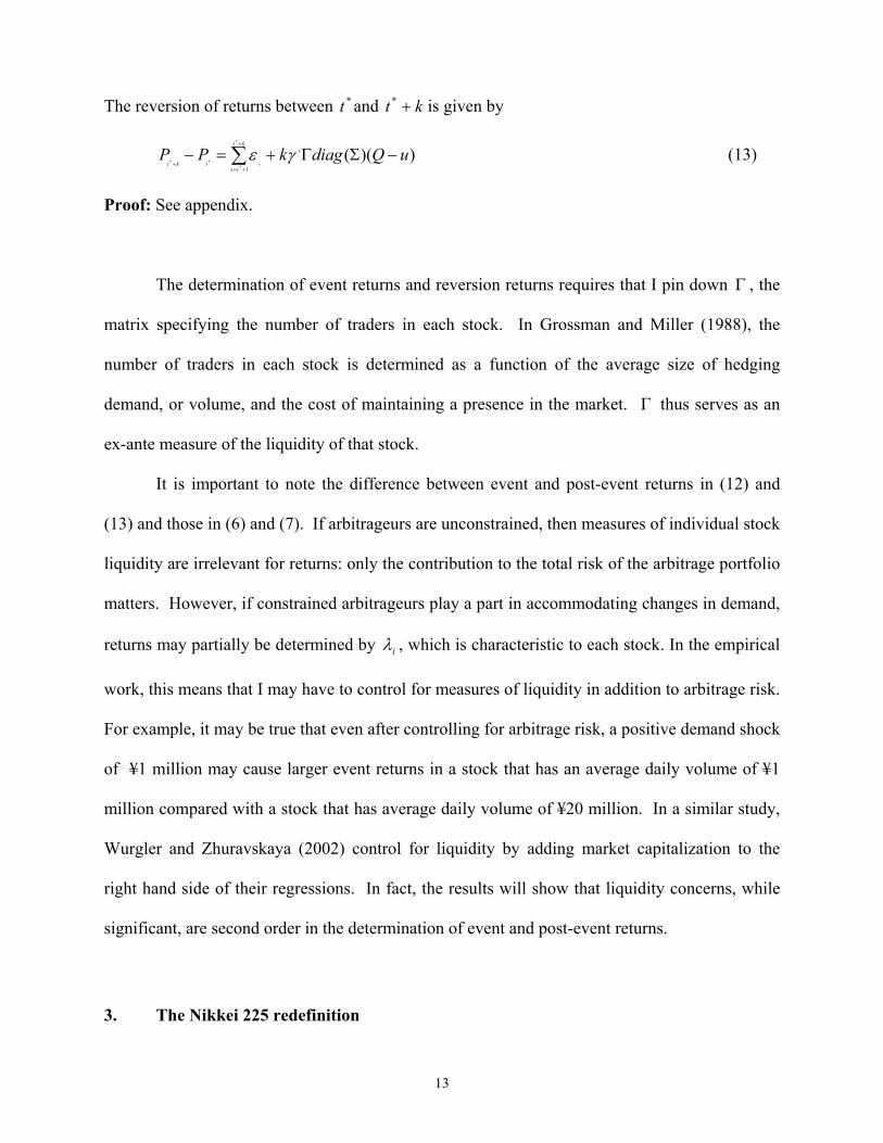
The determination of event returns and reversion returns requires that I pin down Γ , the

matrix specifying the number of traders in each stock. In Grossman and Miller (1988), the

number of traders in each stock is determined as a function of the average size of hedging

demand, or volume, and the cost of maintaining a presence in the market. Γ thus serves as an

ex-ante measure of the liquidity of that stock.

It is important to note the difference between event and post-event returns in (12) and

(13) and those in (6) and (7). If arbitrageurs are unconstrained, then measures of individual stock

liquidity are irrelevant for returns: only the contribution to the total risk of the arbitrage portfolio

matters. However, if constrained arbitrageurs play a part in accommodating changes in demand,

returns may partially be determined by iλ , which is characteristic to each stock. In the empirical

work, this means that I may have to control for measures of liquidity in addition to arbitrage risk.

For example, it may be true that even after controlling for arbitrage risk, a positive demand shock

of ¥1 million may cause larger event returns in a stock that has an average daily volume of ¥1

million compared with a stock that has average daily volume of ¥20 million. In a similar study,

Wurgler and Zhuravskaya (2002) control for liquidity by adding market capitalization to the

right hand side of their regressions. In fact, the results will show that liquidity concerns, while

significant, are second order in the determination of event and post-event returns.

3. The Nikkei 225 redefinition

14

A. Description

The Nikkei 225 is the most widely followed stock index in Japan. The newspaper Nihon

Keizai Shimbun (Nikkei) has maintained the index since 1970, following the discontinuation of

the Tokyo Stock Exchange Adjusted Stock Price Average. The 225 index stocks are selected

according to composition criteria set by Nikkei. Although index guidelines set strict targets for

industry composition and liquidity requirements for individual stocks, changes to index

composition have historically been infrequent. Since the structure of the index had remained

relatively fixed while the industrial composition of the stock market was changing, the Nikkei

had become less representative of the market over time. With the dual aim of reviving the

relevance of the index and cashing in on the hype for new-economy stocks, Nikkei announced on

Friday, April 14, 2000 that rules defining index composition would change. The announcement

cited changes in the “industrial and investment environments” and would become effective one

week from the following Monday, on April 24, 2000.8 Accordingly, for the remainder of the

paper, “event window” refers to returns between April 14 and April 21, and “post-event

window” refers to returns beginning April 24. This chronology is described in Figure 1.

The index redefinition substituted 30 large capitalization stocks for 30 small

capitalization stocks, in addition to significantly downweighting the 195 stocks that remained in

the index. Since the revision became effective on April 24, institutional investors tracking the

Nikkei index had one full week to rebalance their portfolios. Rebalancing was complicated by

the increasing prices of the additions and falling prices of the deletions during this time.

8 A full description of index rules can be found at http://www.nni.nikkei.co.jp/FR/SERV/nikkei_indexes/nifaq225.html#gen1

15

Figure 2 plots the returns of securities affected by the Nikkei 225 index redefinition.

Panel A shows the equally weighted returns of 30 additions, 30 deletions, and 195 remainders

during a one month window surrounding the event. During the five trading days following the

announcement, average returns of the additions diverged dramatically from those of the

remainders and the deletions. Both remainders and deletions experienced negative returns

during that week, with the deletions falling by an extraordinary 30%. Following the event and

the initial returns, prices of additions, deletions and remainders appear to be stable. Panel B

shows the same data at a longer horizon, where there appears to be substantial reversion in prices

at horizons of 10 to 15 weeks.

Table 1 describes the returns of the portfolios shown in Figure 2. On the announcement

day, April 14, returns of the additions, deletions and remainders are all slightly negative. It

appears that the news did not reach the market before the close of trading. On the following

Monday, the deletions fell by an average of 18.81 percent, while the remainders fell by 5.08

percent and the additions were approximately flat. The following day, the additions rose by 7.26

percent while the remainders and deletions continued to fall. By Friday of that week, additions

has risen by 19.13 percent since the previous Friday’s close, while the deletions and remainders

had dropped by 32.29 percent and 13.35 percent, respectively.

The second panel of Table 1 summarizes returns over longer horizons. In the week after

the event, part of the initial event returns was reversed. The additions fell by 6.95 percent, the

deletions gained 0.62 percent and the remainders gained 6.28 percent, about half of what they

had lost during the previous week. In the 10 weeks following the event, additions had a

cumulative return of –9.99 percent, while the deletions and remainders gained 30.13 percent and

16

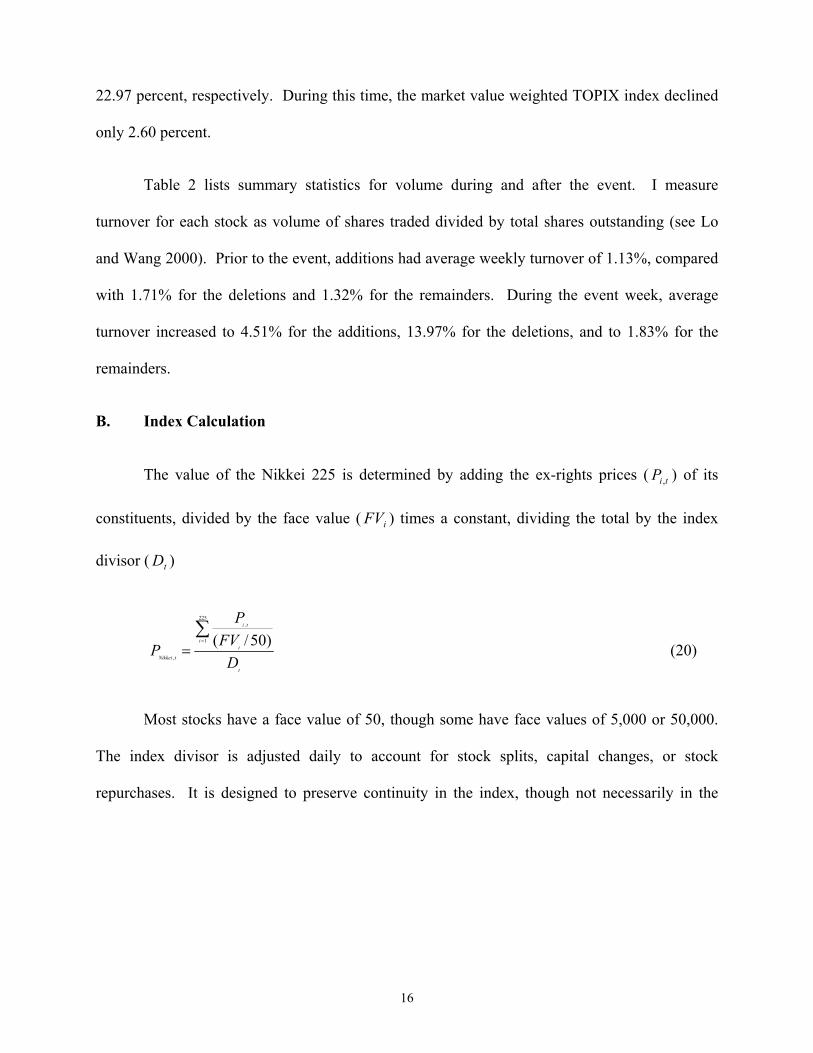
22.97 percent, respectively. During this time, the market value weighted TOPIX index declined

only 2.60 percent.

Table 2 lists summary statistics for volume during and after the event. I measure

turnover for each stock as volume of shares traded divided by total shares outstanding (see Lo

and Wang 2000). Prior to the event, additions had average weekly turnover of 1.13%, compared

with 1.71% for the deletions and 1.32% for the remainders. During the event week, average

turnover increased to 4.51% for the additions, 13.97% for the deletions, and to 1.83% for the

remainders.

B. Index Calculation

The value of the Nikkei 225 is determined by adding the ex-rights prices ( tiP , ) of its

constituents, divided by the face value ( iFV ) times a constant, dividing the total by the index

divisor ( tD )

t

ii

ti

tNikkei DFV

P

P∑=

=

225

1

.

,

)50/( (20)

Most stocks have a face value of 50, though some have face values of 5,000 or 50,000.

The index divisor is adjusted daily to account for stock splits, capital changes, or stock

repurchases. It is designed to preserve continuity in the index, though not necessarily in the

17

index weights of its constituents.9 After adjusting by face value, the index is equally weighted in

prices.

Table 3 describes construction of the index in detail. Calculations are based on prices on

April 14, with the convention that the “old index” (or “post-event” index) includes the 30

deletions and 195 remainders, and the “new index” (or “pre-event” index) includes the 30

deletions and 195 remainders. In the subsequent analysis, net purchases are always calculated

using April 14 prices, although the basic results are unchanged if prices at the end of the

following week are used.10

Table 3 shows that out 30 additions, 26 have a face value of 50. They have an average

price of 5,141, which results in an average weight of 1.46 percent in the post-event index. The

last column of the table shows the Nikkei index weight divided by the weight that the stock

would have taken were the index value-weighted. If the ratio is greater than 1, these stocks are

overweighted in the Nikkei relative to a value-weighted index, while if less than 1, these stocks

are underweighted. For example, in a market-value weighted index, the 26 additions with face

value 50 would have an average weight of 0.46 percent (1.46/3.14). There is one addition with a

face value of 5,000 and a price of 1,090,000 on April 14, 2000. This means that its price must

first be divided by 100 (5,000/50) before being added to the prices of other constituents. This

yields a Nikkei index weight of 3.10, which is 3.87 times the weight it would have taken in a

market-value weighted index. On average, the additions are overweighted in the new index.

9 For example, following a stock split, the effective weight of a stock falls by one half, while the divisor is changed to keep the index value unchanged. 10 Index weights depend on prices. It follows that my estimate of net purchases depends on when I fix prices and total funds linked to the Nikkei. During the rebalancing week, the prices of the additions rose while the prices of the deletions and remainders fell. This increased the weight of the additions in the index further still, increasing the total net purchases during this week. I use beginning-of-the-week prices as a conservative estimate of the size of the shock.

18

Their mean index weight is 1.42 percent, a factor of 2.88 greater than the hypothetical weight in

the market value weighted index.

Similar to the additions, deletions were overweighted in the old Nikkei index..11

Although their average Nikkei weight was only 0.12 percent they would have had an even lower

weight in a market-value weighted index. Because additions had a larger weight in the index

than the deletions (1.46x30=43.8 percent compared with 3.6 percent for the deletions), the total

weight of the 195 remainders fell. The total weight of the remainders fell from 95.6 percent

(0.49*195) to 56.6 percent (0.29*195), a drop of about 40 percent. Effectively, this meant that

institutions tracking the Nikkei index had to sell 40% of their entire holdings simply to purchase

the additions in the correct proportion.

C. Calculation of the demand shock vector

An institutional investor tracking the performance of the index would have rebalanced

her portfolio with current Yen value K to match the composition of the new index. Denote the

Yen weight of security i in the index portfolio as

t

jj

tj

ji

i

DFV

PFVP

w∑

=

=225

1

,

)50/(

)50//(

(21)

wi can be interpreted as the cash value of stock i held by an investor who owns 1 Yen worth of

the index. Denoting total index capital by K, Kwi is cash amount of a stock i tied to the index,

11 Note that since I am computing equally weighted averages, it is possible (and indeed occurs) for the average stock to be overweighted in the index. By definition, the market-value weighted overweighting is equal to 1, but the equally weighted average overweighting may be greater than or less than 1. I study equally weighted averages since they are the relevant statistic in the empirical work, in which each firm is given equal weight in the statistical inference.

19

I calculate the effects on wi from a change in index composition under the assumption

that prices remain fixed, thus yielding the size of the demand shock (expressed in yen) of each

security affected by index rebalancing.

Assume that stocks 1…M (M<N) are replaced by 1*…M*. In the case of the Nikkei 225

rebalancing, the sum of the prices of the added securities, normalized by face value, is greater

than the sum of the prices, normalized by face value, of the deleted securities

∑∑ <*

*1

*

1 )50/()50/(M

i

iM

i

i

FVP

FVP

(22)

To calculate new index weights requires a new index divisor. The divisor is adjusted to preserve

continuity in the index. This means that if the index were to close at value θ today, the new

index must be defined such that it would have closed at value θ. I therefore calculate

t

N

i i

ti

t

N

i i

ti

DFV

P

DFV

P

~)50/()50/( 1

,*

1

, ∑∑== =

∑∑

∑∑

+==

+==

+

+

= N

Mi i

tiM

i i

ti

N

Mi i

tiM

i i

tit

t

FVP

FVP

FVP

FVPD

D

1

,

1

,

1

,

1

,*

)50/()50/(

)50/()50/(~

*

*

(23)

The new vector of index weights is given simply by prices, divided by face value, divided by the

new index divisor. For each security i, net purchases (the demand shock) is equal to the old

index weight, minus the new index weight, times the total amount of funds linked to the Nikkei

225 index. Under the assumption that index linked assets total 2,430 billion Yen (about US $24

20

billion), the sum of the absolute value of weight changes, multiplied by total assets, yields a total

demand shock of 2,072 billion yen, approximately US$20billion.12

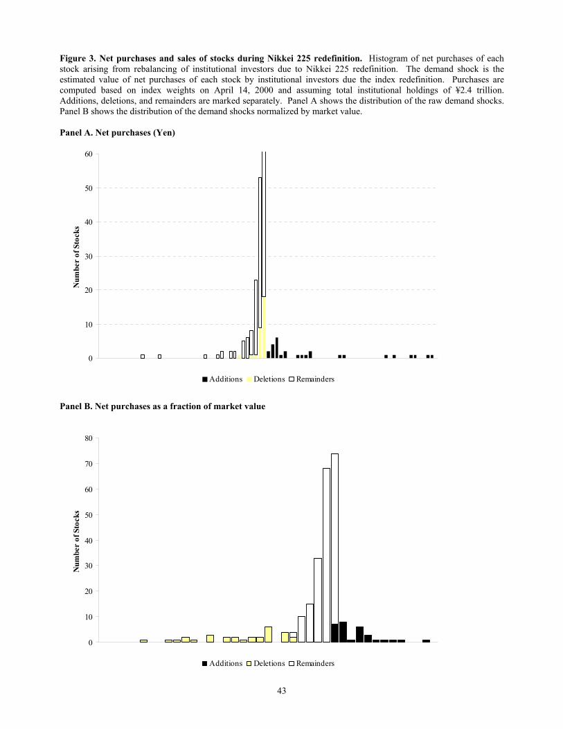
The breakdown of index weights makes it clear where cross-sectional variation in

demand comes from. Figure 3 plots the distribution of net purchases of additions, deletions and

remainders, expressed in yen. The bottom panel plots the histogram of net purchases normalized

by the market value of each stock. The figure reveals that although net sales of the remainders

were high in yen amount, they were lower than the deletions when expressed as a fraction of

market capitalization.

D. Information Content of the Event

Having calculated the net purchases of each security, it is important to ask whether the

demand may have reflected private information. If this were true, event returns may partially be

driven by information about fundamentals.

Generally speaking, index inclusions are a unique setting for the study of demand curves

for stocks because changes in index weight provide no economic information about the future

cash flows of the firms involved. There are two questions. First, do the new index criteria

provide information about future cash flows? Second, if yes, how is this information correlated

with my independent variables in the cross-section?

The new criteria for index selection were (a) components must be from the 450 most

liquid stocks in the first section of the Tokyo Stock Exchange, (b) stocks will be divided into 6

12 Total index linked assets are quoted from Nomura (2000). The demand shock figure corresponds to the sum of absolute values of the demand shocks for each stock. By definition, the sum of the actual values equals zero, since positive shocks by additions are offset by negative shocks by deletions and remainders.

21

sectors, (c) stocks will be chosen individually after selection of sector weights.13 The liquidity of

each security was determined by looking at turnover value and rate of price change per unit of

turnover. However, since criteria for inclusion and exclusion were drawn from publicly

available (price and volume) historical data, the changes gave no new insight into their

fundamentals. Finally, while one can debate whether index inclusion has any effects on future

fundamentals, there are certainly no information effects for the 195 remainders, for which the

weight change occurred only incidentally because of the difference in price between the

additions and deletions.14 In the results that follow, it is a useful robustness check to verify that

all of the major findings hold on both the full sample of 255 stocks, as well as the sub-sample of

195 remainders.

To answer the second question, information is less of a concern in a cross-sectional study,

unless innovations in fundamentals are systematically related to the independent variables. In

this paper, it is difficult to argue that cross-sectional variation of demand shocks is related to

variation in news about their fundamentals.

4. The cross-section of event returns

A. Estimation

In most event studies, the statistical issue of greatest concern is calculating what returns

would have been if the event had not occurred. Particularly in long-horizon studies, the results

frequently rest on assumptions about the equilibrium rate of return.15

13 These were taken from http://www.nni.nikkei.co.jp/FR/FEAT/plunge/plunge0095.html 14 This is similar, but with more securities, to the event described in Kaul, Morck and Stangeland (2000). 15 In long-horizon studies, results are often substantially different when cumulative abnormal returns are used rather than buy-and-hold returns.

22

Campbell, Lo and Mackinlay (1996) report two standard corrections for market

movements. First, one can simply subtract the market return from event returns. Since this is a

single event and the window includes the same days for all securities, subtracting the market

return only changes the constant term in the cross-sectional regressions. The second technique is

to estimate pre-event betas and subtract the appropriate risk premium for each stock. However,

most of the market return during the week was driven by the returns of the Nikkei index,

invalidating this technique. It is conceivable that pre-event betas be estimated on non-event

stocks (about 20-30% of the market), but I use raw returns to keep matters simple. As a

robustness check, I re-estimate all regressions allowing for cross-sectional variation in market

risk. Where I study returns at longer horizons, I report both sets of results.

If the number of periods is small relative to the number of data points in the cross section,

assuming the errors are cross-sectionally uncorrelated yields standard errors that are biased

downward by a factor of five (Fama and French (2000)). In this paper, there are few periods

(one event week and 20 weeks of reversion) with 255 points in each cross-section. There are

many standard techniques to deal with this problem. I estimate the average covariance matrix of

returns prior to the event, and calculate GLS standard errors under the assumption that the

covariance matrix of residuals is the same during the event as in the historical data. The benefit

of this technique is that it does not depend on parameter estimates during the event. However,

in some cases this technique reduces standard errors in comparison with ordinary least squares.

This is because the negative relationship between the returns of the additions and the returns of

the deletions during the event week is statistically stronger once one recognizes that the returns

of the additions and deletions are ordinarily positively correlated (OLS would assume that they

are uncorrelated ordinarily). To be conservative, the tables report the greater of OLS and

covariance adjusted standard errors.

23

B. Arbitrage risk and event returns

The model suggests that event returns are linear in the contribution of each demand shock

to the total risk of the arbitrageur’s portfolio. This requires that I calculate the contribution of

each shock to the risk of a diversified portfolio. I follow the model and multiply a proxy for the

covariance matrix of fundamentals by the vector of demand shocks (net purchases), expressed in

yen. This yields an Nx1 vector, of which the ith element represents the marginal contribution of

security i to total arbitrage risk. To proxy for the covariance matrix of fundamentals, I simply

use the historical average covariance matrix of weekly returns prior to the event.16 While the

historical average covariance is perhaps an imperfect measure of the true risk, it likely

corresponds to the technique used by real arbitrageurs in determining the ex-ante riskiness of

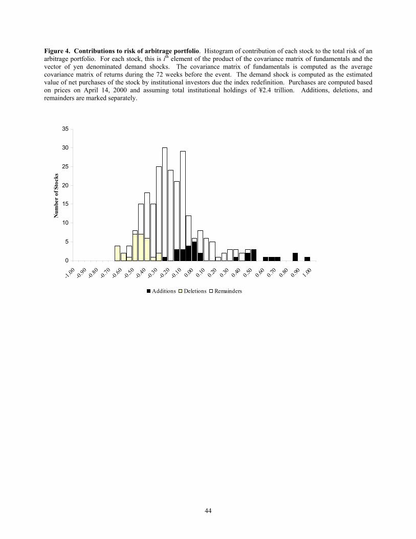
their portfolios. Figure 4 shows a the distribution of this risk measures, including the 30

additions, 30 deletions and 195 remainders. The figure reveals a high degree of cross-sectional

variation both across the three groups of securities, as well as within each group. Note that

there is considerable overlap between the three groups of securities: while most of the additions

have positive contributions to the total risk of the arbitrage portfolio, there are remainders with

greater contributions. This occurs because the additions hedge the risk of some of the positions

forced upon arbitrageurs by the deletions and remainders, reducing their required return.

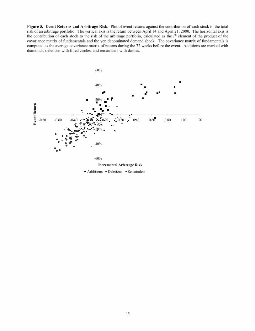
Figure 5 plots event returns against this risk measures for each of the 30 additions, 30

deletions and 195 remainders to the risk of the arbitrage portfolio. The figure reveals a striking

relationship between event returns and the contribution of each stock to the risk of the arbitrage

portfolio. The additions make up most of the top right quadrant, while the deletions and

16 The historical average is computed on 72 weeks of data. The results hold irrespective of my proxy for the covariance matrix of fundamentals. Alternative measures experimented with include the average covariance matrix of daily returns * √5 , and the average covariance matrix of weekly returns at different horizons.

24

remainders make up most of the bottom left quadrant. Close inspection of the figure reveals that

additions, deletions, and remainders all separately confirm the positive linear relationship

between event returns and my risk measure.

Table 4 tests the relationship between arbitrage risk and event returns using the

regression framework from Proposition 2. Specifically, I estimate

iiiiXcXbar ε+Σ∆+∆+= )(

(24)

on the cross-section of event returns. The independent variable iX∆ measures the size of the

demand shock, and Σ is the covariance matrix of fundamental returns. As before, the term

iX )(Σ∆ can be interpreted as the contribution of the demand shock for security i.

Panel A shows a strong relationship between arbitrage risk and event returns. The first

line shows that in the full sample, stocks had high negative returns during the event week. This

return is partly explained (line 2) by the size of the demand shock. However, the coefficient on

the size of the demand shock drops by half when I control for arbitrage risk (line 3). Both the

coefficient on arbitrage risk adjusted shock, and on the size of the demand shock alone are highly

significant. Correcting for market exposure (line 5) does not change the results.

How economically significant are these results? The table shows that the R2 on the

univariate regression of event returns on the arbitrage-risk adjusted demand shock is 0.57, and

rises to 0.60 when I control for unadjusted (by risk) net purchases. In short, more than half of the

variation in returns during this week is explained by demand. Another measure of the economic

importance of portfolio risk is the extent to which it decreases the constant term a in the

regressions. In Panel A, the significance and absolute value of the coefficient falls by about half

once I control for arbitrage risk.

25

Panel B, C and D repeat the baseline regressions in Panel A on the subsets of 30

additions, 30 deletions, and 195 remainders. In every case but for the additions, controlling for

arbitrage risk eliminates the pure effect of the demand shock on event returns.

C. Does arbitrage portfolio risk really drive returns?

The specification in (24) combines the hedging security i provides for other arbitrage

positions with the product of its own shock with its own variance, to yield total arbitrage

portfolio risk. However, it is simple to decompose the term iX )(Σ∆ into its diagonal and off-

diagonal components, thus separating the hedging effect from security i’s diversifiable

contribution to risk. Denoting the ith element of the jth row of Σ as σij, and the ith diagonal term

of Σ as 2iσ , iX )(Σ∆ can be rewritten as

∑≠

∆+∆=Σ∆ij

jijiiiXXX σσ 2)( (25)

Henceforth, let the first and second terms on the right hand side of (25) be known as the hedging

and the unhedged contributions to arbitrage risk, respectively. The decomposition allows for

greater understanding of the results because the coefficient on the unhedged contribution to

arbitrage risk may be open to alternate explanations, while the hedging component is not. For

example, rather than capture the risk contributed to the arbitrage portfolio, 2iσ may be related to

the security’s liquidity. In this case, multiplying the demand shock by the variance normalizes

the demand shock by the ex-ante sensitivity of the stock price to demand.

Substituting (25) into the regression model yields

iij

jijiiiiXdXcbuar εσσ +∆+∆++= ∑

≠

2

(26)

Table 5 shows estimates from this specification for each group of securities. Panel A examines

the results on the entire cross-section of 255 securities. The specification on the third line shows

26

that the results in Table 4 are indeed driven by the hedging contribution to arbitrage risk. In

other words, the idiosyncratic risk of each stock is not the only determinant of the slope of the

demand curve. When I drop the raw demand shock from the regression (line 4), the coefficients

on both diversified and non-diversified arbitrage risk remain significant.

Panels B, C and D repeat the basic specifications from Panel A on the additions,

deletions, and remainders separately. Again, where there were significant results in Table 4, they

appear to be driven by the significance of d, the coefficient on hedged arbitrage risk.

D. Robustness: Controlling for liquidity

The model expresses event and post-event returns as a function of the contribution of the

vector of demand shocks to the total risk of the arbitrage portfolio. However, when one allows

for the presence of constrained arbitrageurs in different measures across stocks, returns may

partially be determined by iλ , which is characteristic to each stock (see Proposition 3). The

importance of liquidity controls is best understood with the following example.

NTT Docomo, a cellular phone company, experienced one of the largest positive Yen

denominated demand shocks in the sample, with total buying estimated at approximately ¥25

billion. This yields a high contribution to the total risk of an arbitrage portfolio, 25th largest in

the sample of 30 additions. However, empirically the effect of the demand on prices may be

mitigated by the fact that the demand shock was but a small multiple of the typical daily trading

volume of this stock—net purchases arising for the rebalancing was less than a single day’s

trading volume.

To control for liquidity, I re-estimate the baseline regression including measures of

liquidity on the right hand side

27

iiiiiiiiMVXeVolXdXcXbar ε+∆+∆+Σ∆+∆+= )/()/()(

(27)

As before, the coefficient c measures the sensitivity of returns to the contribution of the stock to

the risk of an arbitrage portfolio. The regression now includes measures of the demand shock

normalized by liquidity. The first of these is net purchases divided by average trading volume.

The second is net purchases as a fraction of market capitalization.

Table 6 shows these results. In Panel A, the table shows estimates for the entire sample

of securities. The coefficient on the contribution to arbitrage risk falls from 0.396 to 0.281 once

I add the control for liquidity, as proxied by trading volume. The coefficient falls from 0.396 to

0.332 when liquidity is proxied by market capitalization. Nevertheless, controlling for either

measure of liquidity, arbitrage risk remains a significant determinant of event returns.

Panels B, C and D repeat these regressions for the additions, deletions, and remainders

separately. Each panel separately confirms the results in Panel A: the primary determinant of

event returns is the contribution of the demand shock of that stock to the total risk of the

arbitrage portfolio.

E. Post-event returns

Both propositions 2 and 3 predict that the reversal of returns following a demand shock

should occur at a rate proportional to the initial event returns. This is a simple consequence of

event returns reflecting expected future profits of arbitrageurs who initially absorbed the

demand.

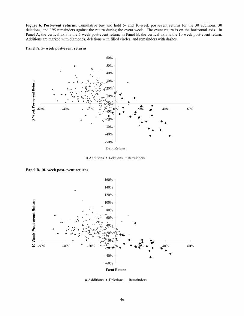
Figure 6 provides some justification for the claim that in the cross-section, post-event

returns are negatively related to event returns. Panel A plots the cumulative 5-week post-event

return for each stock against the return during the event week. Additions, deletions, and

28

remainders are marked separately. The figure shows a negative linear relationship between post-

event returns and event returns. Close inspection reveals that this pattern is borne out within the

additions, deletions, and remainders separately.

Panel B plots the cumulative 10-week post-event return for each stock against the return

during the event week. Again, the Panel shows a negative linear relationship between post-event

and event returns. Naturally, the variability of returns increases at this longer horizon, but the

basic relationship is unchanged.

Table 7a tests the relationship between post-event and event returns shown in Figure 4.

For each week after the event, I regress the cumulative k-week post-event return on the event

return for that stock

ikitkkititrR ελ +=

+ *** ,

(28)

The coefficient λk is interpreted simply as the fraction of event returns that have reverted by week

k. I show estimates for 1, 2, 3, 4, 5, 10, 15 and 20 weeks after the event, with the regression

estimated on both the entire set of securities, and on the additions, deletions, and remainders

separately. The first panel shows that 32% of the initial event returns were reversed in the first

week after the event. After 5 weeks, 57% of the initial event returns had been reversed, while

after 10 weeks, 114% of the event returns were reversed. This pattern is confirmed among the

additions (53% reversion after 10 weeks), deletions (91% reversion after 10 weeks), and

remainders (146% reversion after 10 weeks) separately.

Equation (28) does not include a constant term, imposing strict linearity between event

and post-event returns. As a result, it does not allow for changes in security prices for each

29

group of stocks related to news, such as market-wide information driving all stock prices up or

down. Adding a constant term eliminates this concern. On the other hand, adding a constant

term also eliminates information about the average event return for each group of securities,

while preserving cross-sectional variation within each group,

The second panel of Table 7 shows estimates of this regression

ikitkkkititraR ελ ++=

++ *** ,1

(29)

The λk estimates now reflect reversion of cross-sectional variation within each group of securities

and do not capture the average reversion of the group of additions, deletions, and remainders.

Nevertheless, the results hold as before. For the group of all securities, 30% of cross-sectional

variation in returns is reversed within one week of the event, and 84% within 10 weeks of the

event. This pattern again holds within the additions, deletions, and remainders, with 70%, 56%

and 96% of event returns reversed within 10 weeks of the event.

Figure 6 traces the time series of estimates of λk from (28) and (29), estimated on the

entire sample. Panel A plots estimates from the regression that includes a constant term and

Panel B shows estimates from the regression in which the constant term is omitted.

The first panel shows that event returns reverted at a faster pace during the first 4 weeks

after the event, after which the rate of reversion slowed. Dropping the constant term in Panel B

does not change the basic pattern of post-event reversion.

The assumption that the equilibrium rate of return is zero is more problematic at long

horizons, and may bias the results I report in Table 7a. As a robustness check, I re-estimate the

regressions in Table 7a using a measure of excess post-event returns as the dependent variable. I

calculate pre-event betas with respect to the market value weighted TOPIX index using data 52

weeks before the event, and adjust post-event returns with these betas. I then study post-event

30

excess returns as a function of the event return. These results are shown in Table 7b. Over

longer horizons, the adjustment strengthens the results.

5. The profitability of arbitrage strategies

While the reversion documented in this paper is consistent with positive expected returns

to arbitrage, little has been said thus far about the ex-post profitability of arbitrage strategies

during the Nikkei 225 rebalancing. In single event studies, calculation of arbitrage profits

requires a good understanding of how arbitrageurs hedge their short positions in additions or

long positions in deletions. Wurgler and Zhurvaskaya (2002) document that such hedging is

difficult in practice and still involves considerable idiosyncratic risk. They show that the

idiosyncratic risk is an important determinant of the event return in the first place.

In the Nikkei 225 redefinition, calculation of the arbitrage portfolio is trivial. Since net

purchases of the additions were exactly offset by net sales of the deletions and remainders,

arbitrageurs simply accommodated the entire demand vector.17 Of course, this portfolio may still

have some market risk. I therefore consider the profits of two alternate strategies. The first

strategy simply accommodates the demand shock without hedging market risk. Panel A of

Figure 8 shows the buy-and-hold value of the portfolio that is short 30 additions and long 30

deletions and 195 remainders in proportion to index weights based on prices on Friday, April 14,

2000. On this day, the cost of the deletions and remainders exactly offset the proceeds from the

additions; thus the value of the portfolio is zero. The profits indicated on the vertical axis

correspond to those of an arbitrageur who absorbed 1% of the total demand induced by

institutional rebalancing, under the assumption that institutional funds linked to the Nikkei are

17 This was also confirmed by the author in an interview with Taro Hornmark, an arbitrageur during this event.

31

assumed to equal ¥2.4 trillion.18 The minimum value occurs on April 21, at which point the

portfolio has declined in value by ¥4.17 billion. Because I lack data on the cost of short selling, I

am unable to adjust this figure to reflect transactions costs. However, this adjustment would

make the loss even more severe.

The second strategy I consider is one that accommodates the demand shock but hedges

exposure of the arbitrage portfolio to market movements. This is done as follows. I calculate

pre-event betas with respect to the TOPIX index for each of the 255 stocks using 52 weeks of

pre-event weekly returns. The market beta of the unhedged portfolio is the sum of these betas,

weighted by estimated net purchases, on April 14, 2000. The hedged arbitrage portfolio is equal

to the unhedged portfolio minus the market beta times the topix index.

Figure 8 shows profits from this portfolio. The figure demonstrates that the market risk

adjustment does little to change the profitability of the arbitrage portfolio.

A notable feature of both portfolios is that after the initial drop in value during the event

week, the value of each reverts quickly to zero. Nevertheless, both strategies involved

considerable risk, as the figure displays week-to-week fluctuations of more than ¥0.3 billion.

Finally, it is important to recognize that the profitability of arbitrage strategies during the

event occurred at the expense of institutions that were forced to trade at April 21 prices. The

figure reveals that if the institutions had been willing to wait 10 weeks or more after the event

before rebalancing, they could have avoided a loss of ¥4 billion. Since the figure represents only

1 percent of total estimated rebalancing, this implies a transfer of wealth of approximately ¥400

billion to arbitrageurs.

6. Conclusions 18 Nomura (2000).

32

The transfer of wealth from institutional investors to arbitrageurs during the Nikkei 225

redefinition highlights the importance of working arbitrage. While the event conveyed no

economic news, it transferred significant wealth to investors willing to wait 10 to 20 weeks

before rebalancing.

Not only did the redefinition cause a lot of trading, the trading displayed wide variation in

the cross-section of stocks. This paper uses this variation to understand the dynamic effects of

demand shocks on prices. In a simple model, I show that following a change in the net supply of

assets, event returns are proportional to the contribution of each shock to the risk of a diversified

arbitrage portfolio. The model also predicts that post-event returns are negatively correlated with

the initial event return. Both predictions are strongly supported by the data.

33

Appendix A. Model

The capital market includes N risky securities in fixed supply with supply vector given by

Q. The risk-free asset is in perfectly elastic supply with net return normalized to zero. Each

security pays a liquidating dividend at some time T. The information flow regarding dividend

TiD , is given by

∑=

+=t

ssiiti DD

1,0,, ε i∀ (A1)

in which the information shocks ti ,ε are identically and independently distributed over time and

are normal with zero mean and covariance matrix Σ .

A. Unconstrained solution

Arbitrageurs maximize exponential utility of next period wealth subject to a wealth

constraint:

( )[ ]1expmax +−− ttNWE γ (A2)

s.t. [ ]ttttt PPNWW −′+= ++ 11

tW , tP , and tN are arbitrageurs’ wealth, the vector of security prices, and the arbitrageur

demand vector at period t, respectively.

First, solve for prices and returns when *tt < . Demand is given by

tttttT PPEPVarN −= +−

+ )()]([11

11γ

(A3)

In the covariance stationary equilibrium, VPVar tt =+ )( 1 . Then

VQPEP ttt γ−= + )( 1 (A4)

34

Iterating forward and substituting )()( TtTt DEPE = , we get

VQtTDEP Ttt γ)()( −−= (A5)

Now, note that

1

111 )()()(

+

+++

=−=−

t

TtTtttt DEDEPEPε

Multiplying both sides by their transposes, it follows that the expected future variance of prices,

V, is equal to the covariance matrix of fundamentals, Σ . Substituting back into the equation for

prices, this gives

QtTDEP Ttt Σ−−= γ)()( (A6)

Consider the effects of a permanent shock u (Nx1) to the supply of net assets. Substituting

)( uQ − for Q in the above,

)()()( *** uQtTDEP Ttt −Σ−−= γ (A7)

The event return is given by

QutT

QtTuQtTDEDEPP

t

TtTttt

Σ+Σ−+=

Σ+−+−Σ−−−=−

γγε

γγ

)(

)1()()()()(*

**

*

****

(A8)

The reversion of event returns between periods )1( * +t and )( * kt + is given by

)()()()()()( ****** uQtTuQktTDEDEPP TtTkttkt −Σ−+−Σ−−−−=−

++γγ

)(*

* 1

uQkkt

tss −Σ+= ∑

+

+=

γε (A9)

The expected reversion is thus

)(*** , uQkPE kttt −Σ=∆+

γ (A10)

Proposition 1 follows directly from (8) and (10).

35

Finally, note that expected returns in absence of the demand shock would have been

given by

QkPE kttNoShockt Σ=∆+

γ*** ,| (A11)

Therefore, excess reversion returns are simply given by uk Σγ , intuitively, the risk of the

rebalancing portfolio.

We can also construct the unconditional covariance of the vector of reversion returns

with the vector of event returns. First, noting that

∑+

+=+

Σ−=∆−

Σ−=∆−

kt

tsskt

t

ukPEP

utTPEP

t

t

*

***

**

1

*)(

γε

γ

gives

Σ⋅⋅Σ−−=

Σ−⋅Σ−=∆∆ ∑

+

+=−+−

)'()(

]'[])[(),(cov

2*

1

*1,1

*

******

uuEktT

ukutTEPPkt

tsstktttt

γ

γεγ (A12)

Lemma 1. If the matrix A is symmetric positive semi-definite, then for any Nx1 vector x, the

matrix AAxxZ '= is positive semi-definite.

Proof. Write the matrix A in Cholesky form 'LLA = . Then '''' cLLLLxxLLZ == where c is

weakly positive. Positive semi-definiteness follows immediately.

From Lemma 1, the diagonal entries of ΣΣ uEu' must be greater than zero. In short, for each

stock i, own event returns are negatively correlated with reversion returns.

It is also possible to analyze the average cross-sectional covariance between the Nx1

vector of event returns and reversion returns. Consider the ordinary least squares estimator of

the regression of kttP+

∆ ** , on *tP∆ . The slope coefficient is given by

36

[ ] ( )[ ]

)(

')(])[(]')[(

),()]([

*

22*1*2*

,1

1, *******,*

tTk

uuEtTkutTutT

PPCovPVartkttttPP

tktt

−−

=

Σ−−Σ−Σ−=

∆∆∆=

−

+−

−∆∆+

γγγ

β

(A13)

Proposition 2 follows from (8) and (13).

B. Constrained solution

Suppose now that there are N groups of specialized investors, who invest optimally

except that they are constrained to invest in only one asset. Like the unconstrained arbitrageurs,

they maximize exponential utility of next period wealth subject to a wealth constraint. Denoting

demand by specialists as SpecialistitN , for each security i, this yields the demand function

)(

)(1

1

+

+ −=

ittS

itittSpecialistit PVar

PPENγ

(A14)

Suppose that arbitrageurs of this type exist in measure iλ for each security i. Allowing iλ to

differ across stocks is equivalent to allowing for variation in the slope of the underlying demand

curve. This yields the specialist demand vector

−

−

=

+

+

+

+

)()(

)()(

1

1

11

1111

NttS

NtNttN

ttS

ttt

Specialistt

PVarPPE

PVarPPE

N

γλ

γλ

M (A15)

Drawing the demand curve as expected returns on the y-axis and the size of the shock on the x-

axis, the slope is given by )()/( 1+ittiS PVarλγ . Intuitively, demand is flatter the lower the

fundamental risk of the stock, and the higher the quantity of arbitrageurs specialized in that

stock, iλ .

37

Equilibrium in the capital market sets specialist arbitrageur demand equal to total supply.

For each security i, this implies

( ) iitittitt

Si QPPEPVar

=−++

)()( 1

1γλ (A16)

We proceed as in (4), (5), and (6) to get the price of security i as a function of expected dividends

and total supply

QtTDEP iS

iTitit σλγ )/)(()( −−= (A17)

Event returns are given by

iiiiiS

ititit QutTPP 22* )/)((*** γσσλγε +−+=− (A18)

In matrix form, event returns can be written as

QdiagudiagtTPP Sttt )()()( *

*** Σ+ΣΓ−+=− γγε

where Γ denotes the diagonal matrix of random coefficients iλ and )(Σdiag denotes the matrix

containing only the diagonal elements of the variance-covariance matrix of fundamentals Σ .

The reversion of event returns between periods )1( * +t and )( * kt + is given by

)()/( 2

1

*

*** iiii

skt

tsitkit

uQkPPis

−+=− ∑+

+=+

σλγε (A19)

This can also be written in matrix form

))((*

***

1

uQdiagkPP skt

tstkt s

−ΣΓ+=− ∑+

+=+

γε (A20)

38

Appendix B. Units of Measurement

B.1. Regression Units

The main results of the model express the change in price as a function of supply,

expressed as a number of shares. However, the empirical results study returns as a function of

the demand shock, expressed in Yen. To go from one to the other, rewrite (A11) as

QPPEtt PPtt

21 1

)( −+ +=− γσ (B1)

where Q is the number of shares, and 1+tP and tP denote the price, in yen. To get from here to

returns, divide by tP

t

PP

t

tt

PQ

PPPE tt

21 1)( −+ +=− γσ

(B2)

The trick is to note that

22211 tt

t

tt PPtP

PP P −− ++= σσ (B3)

and so (B2) becomes

QPP

PPE

t

tt

PPP

t

tt ⋅=−

−+

+

211

)( γσ (B4)

Returns are linear in the quantity, expressed in Yen (or dollars), and the standard deviation of

returns.

39

References

Barberis, N, and A. Shleifer (2002), Style Investing, Journal of Financial Economics, forthcoming.

Barberis, N, A. Shleifer, and J. Wurgler (2001), Comovement, Mimeo University of Chicago.

Dhillon, U., and Johnson, H (1991), Changes in the Standard and Poor’s 500 List. Journal of Business 64:75-85.

Fama, Eugene F., and Kenneth R. French, 2000, Forecasting profitability and earnings, Journal of Business 73, 161–175.

Froot, K., and E. Dabora (1999), How are Stock Prices affected by the Location of Trade?, Journal of Financial Economics 53, 189-216.

Goetzmann, W., and Garry, M., 1986, Does delisting from the S&P 500 affect stock price? Financial Analysts Journal 42:64-69.

Greene, W., (1997), Econometric Analysis, Prentice-Hall, NJ.

Grossman, Sanford J. and Merton H Miller, Liquidity and market structure, The Journal of Finance 43(3), 617-633.

Hardouvelis, Gikas, Rafael La Porta, and Thierry A. Wizman, "What Moves the Discount on Country Equity Funds?" in Jeffrey Frankel ed.: The Internationalization of Equity Markets (University of Chicago Press, Chicago, IL), 345-397.

Hong, H and J Stein(1999), A unified theory of underreaction, momentum trading and overreaction in asset markets, Journal of Finance 54, 2143-2184;

Harris, L, S&P 500 Cash Stock Price Volatilities, Journal of Finance 44(5), 1155-1175.

Lo, A. and J. Wang, 2000, Trading Volume: Definitions, Data Analysis, and Implications of Portfolio Theory, Review of Financial Studies 13, 257-300.

Lynch, Anthony, and Richard Mendenhall (1997), New evidence on stock price effects associated with changes in the S&P 500 Index, Journal of Business 70(3), 351-383.

Kaul, A., Mehrotra V., and R. Morck (2000), Demand Curves for Stocks Do Slope Down: New Evidence from an Index Weights Adjustment, Journal of Finance 55, 893-912.

Merton, Robert (1987), A Simple model of capital market equilibrium with incomplete information, Journal of Finance 42(3), 483-510.

Randall Morck, Bernard Yeung, and Wayne Yu, (2001) Why Do Stock Prices in Emerging Markets Move in Tandem? Journal of Finance

40

Petajisto, Antti (2003), What makes demand curves for stocks slope down? Mimeo MIT.

Pindyck, R, and J. Rotemberg (1993), The Comovement of Stock Prices, Quarterly Journal of Economics 108(4), 1073-1104.

Shleifer A. (1986), Do Demand Curves for Stocks Slope Down? Journal of Finance 41, 579-590.

Shleifer A. (2000), Inefficient Markets: An Introduction to Behavioral Finance, Oxford University Press, Oxford.

Wurgler, J., and K. Zhuravskaya (2002), Does Arbitrage Flatten Demand Curves for Stocks? Journal of Business.

41

Figure 1. Chronology. Nihon Keizai Shimbun (Nikkei) announced the redefinition of the Nikkei 225 index around the close of the Tokyo stock exchange on Friday April 14, 2000. The redefinition replaced 30 index securities and downweighted the remaining 195 securities. The change became effective when the market opened on April 24, 2000. To minimize tracking error, index traders would have submitted market close orders on Friday April 21, 2000, or market open orders on Monday, April 24, 2000. Accordingly, event returns are defined on the window beginning on the close on April 14 and ending on the close on April 21. Weekly post-event windows are defined beginning on April 24. Date Weekday Event April 13, 2000 Thursday April 14, 2000 Friday Announcement Day April 17, 2000 Monday Institutions begin

April 18, 2000 Tuesday rebalancing April 19, 2000 Wednesday Event Window April 20, 2000 Thursday April 21, 2000 Friday Last day to Rebalance April 24, 2000 Monday Redefinition Effective

April 25, 2000 Tuesday April 26, 2000 Wednesday Post-event window April 27, 2000 Thursday April 28, 2000 Friday

42

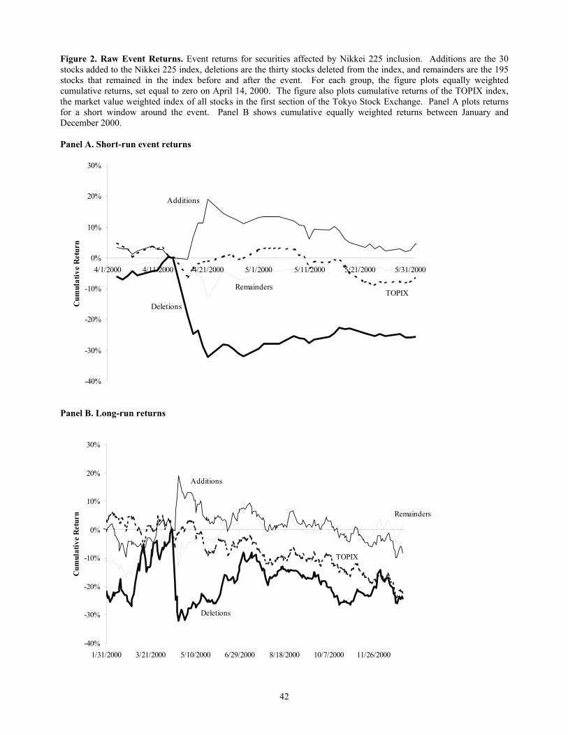
Figure 2. Raw Event Returns. Event returns for securities affected by Nikkei 225 inclusion. Additions are the 30 stocks added to the Nikkei 225 index, deletions are the thirty stocks deleted from the index, and remainders are the 195 stocks that remained in the index before and after the event. For each group, the figure plots equally weighted cumulative returns, set equal to zero on April 14, 2000. The figure also plots cumulative returns of the TOPIX index, the market value weighted index of all stocks in the first section of the Tokyo Stock Exchange. Panel A plots returns for a short window around the event. Panel B shows cumulative equally weighted returns between January and December 2000. Panel A. Short-run event returns

-40%

-30%

-20%

-10%

0%

10%

20%

30%

4/1/2000 4/11/2000 4/21/2000 5/1/2000 5/11/2000 5/21/2000 5/31/2000

Cum

ulat

ive

Ret

urn

Deletions

TOPIXRemainders

Additions

Panel B. Long-run returns

-40%

-30%

-20%

-10%

0%

10%

20%

30%

1/31/2000 3/21/2000 5/10/2000 6/29/2000 8/18/2000 10/7/2000 11/26/2000

Cum

ulat

ive

Ret

urn

Deletions

TOPIX

Remainders

Additions

43

Figure 3. Net purchases and sales of stocks during Nikkei 225 redefinition. Histogram of net purchases of each stock arising from rebalancing of institutional investors due to Nikkei 225 redefinition. The demand shock is the estimated value of net purchases of each stock by institutional investors due the index redefinition. Purchases are computed based on index weights on April 14, 2000 and assuming total institutional holdings of ¥2.4 trillion. Additions, deletions, and remainders are marked separately. Panel A shows the distribution of the raw demand shocks. Panel B shows the distribution of the demand shocks normalized by market value. Panel A. Net purchases (Yen)

0

10

20

30

40

50

60

Num

ber

of S

tock

s

Additions Deletions Remainders

Panel B. Net purchases as a fraction of market value

0

10

20

30

40

50

60

70

80

Num

ber

of S

tock

s

Additions Deletions Remainders

44

Figure 4. Contributions to risk of arbitrage portfolio. Histogram of contribution of each stock to the total risk of an arbitrage portfolio. For each stock, this is ith element of the product of the covariance matrix of fundamentals and the vector of yen denominated demand shocks. The covariance matrix of fundamentals is computed as the average covariance matrix of returns during the 72 weeks before the event. The demand shock is computed as the estimated value of net purchases of the stock by institutional investors due the index redefinition. Purchases are computed based on prices on April 14, 2000 and assuming total institutional holdings of ¥2.4 trillion. Additions, deletions, and remainders are marked separately.

0

5

10

15

20

25

30

35

-1.00-0.90

-0.80-0.70

-0.60-0.50

-0.40-0.30

-0.20-0.10

0.00 0.10 0.20 0.30 0.40 0.50 0.60 0.70 0.80 0.90 1.00

Num

ber

of S

tock

s

Additions Deletions Remainders

45

Figure 5. Event Returns and Arbitrage Risk. Plot of event returns against the contribution of each stock to the total risk of an arbitrage portfolio. The vertical axis is the return between April 14 and April 21, 2000. The horizontal axis is the contribution of each stock to the risk of the arbitrage portfolio, calculated as the ith element of the product of the covariance matrix of fundamentals and the yen denominated demand shock. The covariance matrix of fundamentals is computed as the average covariance matrix of returns during the 72 weeks before the event. Additions are marked with diamonds, deletions with filled circles, and remainders with dashes.

-60%

-40%

-20%

0%

20%

40%

60%

-0.80 -0.60 -0.40 -0.20 0.00 0.20 0.40 0.60 0.80 1.00 1.20

Incremental Arbitrage Risk

Eve

nt R

etur

n

Additions Deletions Remainders

46

Figure 6. Post-event returns. Cumulative buy and hold 5- and 10-week post-event returns for the 30 additions, 30 deletions, and 195 remainders against the return during the event week. The event return is on the horizontal axis. In Panel A, the vertical axis is the 5 week post-event return; in Panel B, the vertical axis is the 10 week post-event return. Additions are marked with diamonds, deletions with filled circles, and remainders with dashes. Panel A. 5- week post-event returns

-50%

-40%

-30%

-20%

-10%

0%

10%

20%

30%

40%

50%

60%

-60% -40% -20% 0% 20% 40% 60%

Event Return

5 W

eek

Post

-eve

nt R

etur

n

Additions Deletions Remainders

Panel B. 10- week post-event returns

-60%

-40%

-20%

0%

20%

40%

60%

80%

100%

120%

140%

160%

-60% -40% -20% 0% 20% 40% 60%

Event Return

10 W

eek

Post

-eve

nt R

etur

n

Additions Deletions Remainders

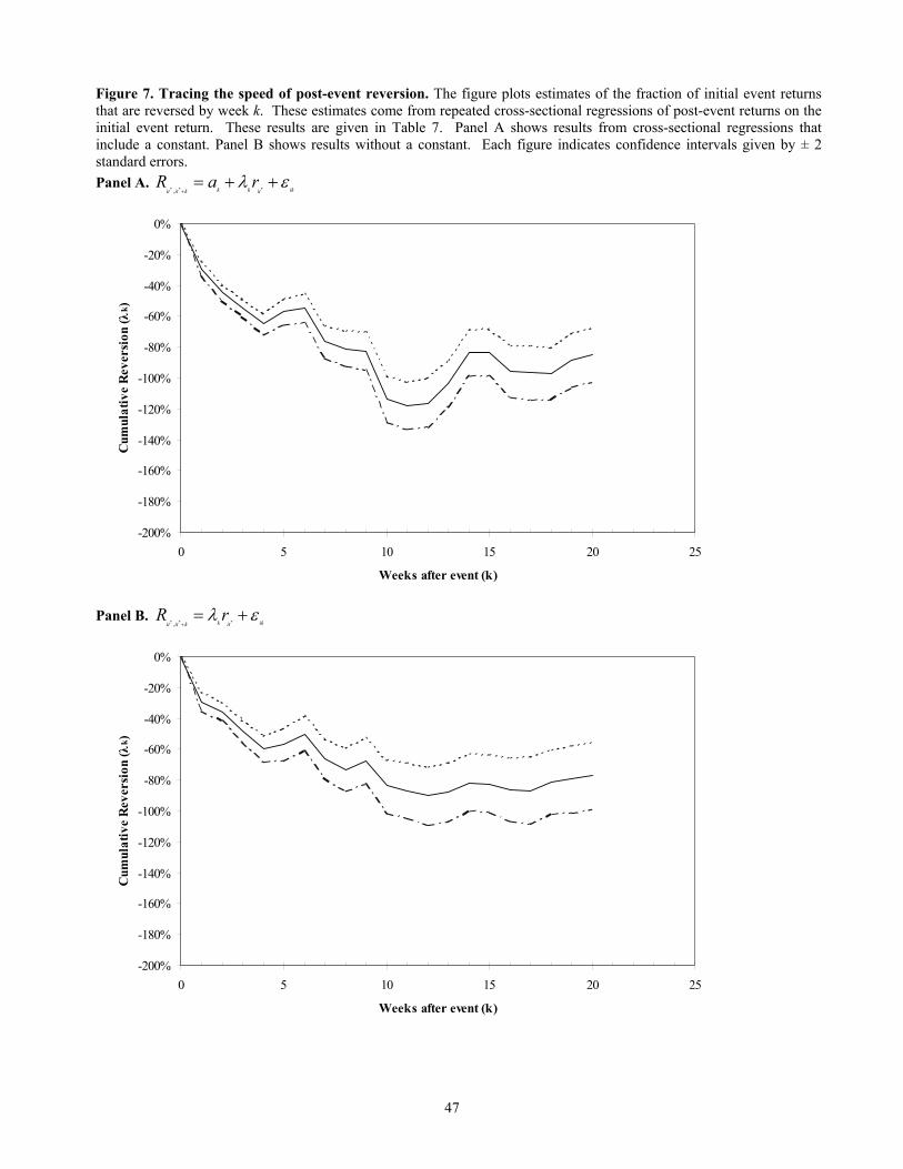
47

Figure 7. Tracing the speed of post-event reversion. The figure plots estimates of the fraction of initial event returns that are reversed by week k. These estimates come from repeated cross-sectional regressions of post-event returns on the initial event return. These results are given in Table 7. Panel A shows results from cross-sectional regressions that include a constant. Panel B shows results without a constant. Each figure indicates confidence intervals given by ± 2 standard errors. Panel A.

ikitkkkitit

raR ελ ++=+ *** ,

-200%

-180%

-160%

-140%

-120%

-100%

-80%

-60%

-40%

-20%

0%

0 5 10 15 20 25

Weeks after event (k)

Cum

ulat

ive

Rev

ersi

on (λ

k )

Panel B.

ikitkkititrR ελ +=

+ *** ,

-200%

-180%

-160%

-140%

-120%

-100%

-80%

-60%

-40%

-20%

0%

0 5 10 15 20 25

Weeks after event (k)

Cum

ulat

ive

Rev

ersi

on (λ

k )

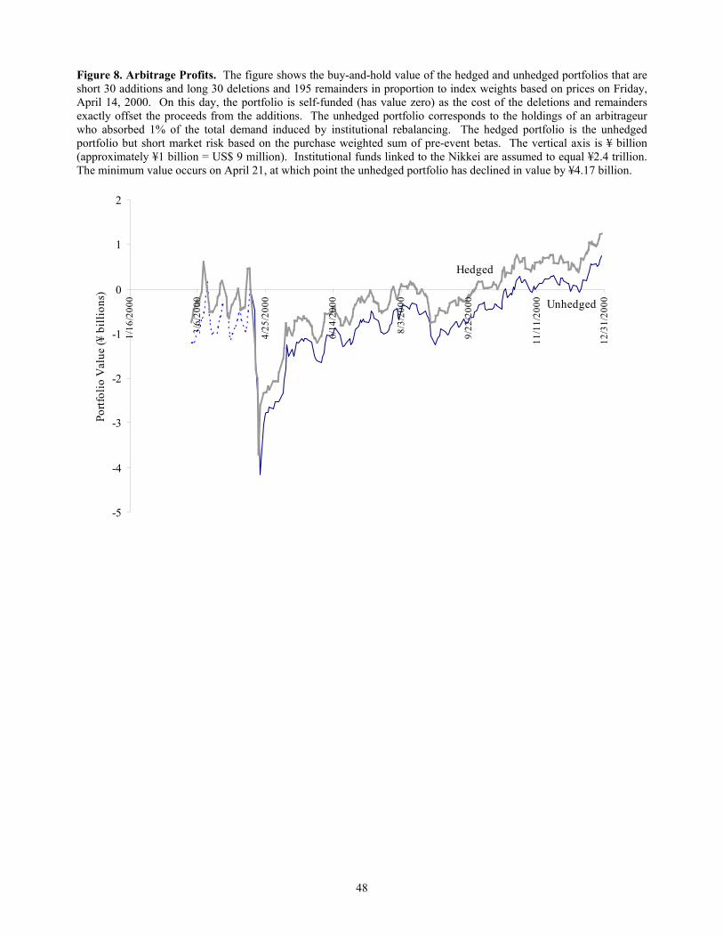
48

Figure 8. Arbitrage Profits. The figure shows the buy-and-hold value of the hedged and unhedged portfolios that are short 30 additions and long 30 deletions and 195 remainders in proportion to index weights based on prices on Friday, April 14, 2000. On this day, the portfolio is self-funded (has value zero) as the cost of the deletions and remainders exactly offset the proceeds from the additions. The unhedged portfolio corresponds to the holdings of an arbitrageur who absorbed 1% of the total demand induced by institutional rebalancing. The hedged portfolio is the unhedged portfolio but short market risk based on the purchase weighted sum of pre-event betas. The vertical axis is ¥ billion (approximately ¥1 billion = US$ 9 million). Institutional funds linked to the Nikkei are assumed to equal ¥2.4 trillion. The minimum value occurs on April 21, at which point the unhedged portfolio has declined in value by ¥4.17 billion.

-5

-4

-3

-2

-1

0

1

2

1/16

/200

0

3/6/

2000

4/25

/200

0

6/14

/200

0

8/3/

2000

9/22

/200

0

11/1

1/20

00

12/3

1/20

00

Portf

olio

Val

ue (¥

bill

ions

)

Hedged

Unhedged

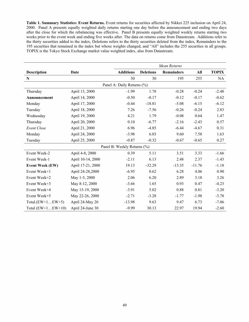
49

Table 1. Summary Statistics: Event Returns. Event returns for securities affected by Nikkei 225 inclusion on April 24, 2000. Panel A presents equally weighted daily returns starting one day before the announcement and ending two days after the close for which the rebalancing was effective. Panel B presents equally weighted weekly returns starting two weeks prior to the event week and ending five weeks after. The data on returns come from Datastream. Additions refer to the thirty securities added to the index, Deletions refers to the thirty securities deleted from the index, Remainders to the 195 securities that remained in the index but whose weights changed, and “All” includes the 255 securities in all groups. TOPIX is the Tokyo Stock Exchange market value weighted index, also from Datastream. Mean Returns Description Date Additions Deletions Remainders All TOPIX N 30 30 195 255 NA

Panel A: Daily Returns (%) Thursday April 13, 2000 -1.99 1.78 -0.28 -0.24 -2.48 Announcement April 14, 2000 -0.50 -0.17 -0.12 -0.17 -0.62 Monday April 17, 2000 -0.44 -18.81 -5.08 -6.15 -6.12 Tuesday April 18, 2000 7.26 -7.56 -0.26 -0.24 2.83 Wednesday April 19, 2000 4.21 1.79 -0.08 0.64 1.47 Thursday April 20, 2000 0.10 -6.77 -2.16 -2.43 0.57 Event Close April 21, 2000 6.96 -4.85 -6.44 -4.67 0.31 Monday April 24, 2000 -3.98 6.03 9.60 7.58 1.63 Tuesday April 25, 2000 -0.87 -0.32 -0.67 -0.65 0.27

Panel B: Weekly Returns (%) Event Week-2 April 4-8, 2000 0.39 5.11 3.51 3.33 -1.66 Event Week-1 April 10-14, 2000 -2.11 6.13 2.48 2.37 -1.43 Event Week (EW) April 17-21, 2000 19.13 -32.29 -13.35 -11.76 -1.18 Event Week+1 April 24-28,2000 -6.95 0.62 6.28 4.06 0.90 Event Week+2 May 1-5, 2000 2.06 6.20 2.89 3.18 3.26 Event Week+3 May 8-12, 2000 -3.66 1.65 0.93 0.47 -4.23 Event Week+4 May 15-19, 2000 -3.91 5.02 0.88 0.81 -3.20 Event Week+5 May 22-26, 2000 -2.71 -3.28 -1.77 -1.98 -3.78 Total.(EW+1…EW+5) April 24-May 26 -13.98 9.63 9.47 6.73 -7.06 Total (EW+1…EW+10) April 24-June 30 -9.99 30.13 22.97 19.94 -2.60

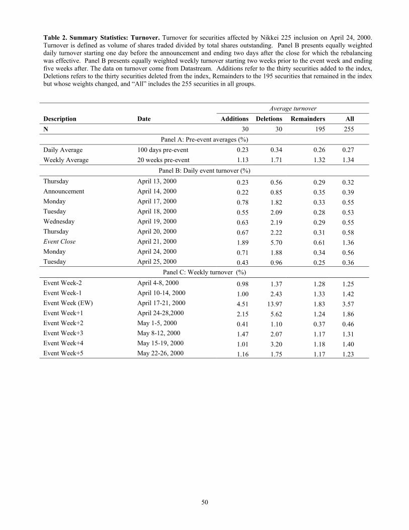
50

Table 2. Summary Statistics: Turnover. Turnover for securities affected by Nikkei 225 inclusion on April 24, 2000. Turnover is defined as volume of shares traded divided by total shares outstanding. Panel B presents equally weighted daily turnover starting one day before the announcement and ending two days after the close for which the rebalancing was effective. Panel B presents equally weighted weekly turnover starting two weeks prior to the event week and ending five weeks after. The data on turnover come from Datastream. Additions refer to the thirty securities added to the index, Deletions refers to the thirty securities deleted from the index, Remainders to the 195 securities that remained in the index but whose weights changed, and “All” includes the 255 securities in all groups. Average turnover Description Date Additions Deletions Remainders All N 30 30 195 255

Panel A: Pre-event averages (%) Daily Average 100 days pre-event 0.23 0.34 0.26 0.27 Weekly Average 20 weeks pre-event 1.13 1.71 1.32 1.34

Panel B: Daily event turnover (%) Thursday April 13, 2000 0.23 0.56 0.29 0.32 Announcement April 14, 2000 0.22 0.85 0.35 0.39 Monday April 17, 2000 0.78 1.82 0.33 0.55 Tuesday April 18, 2000 0.55 2.09 0.28 0.53 Wednesday April 19, 2000 0.63 2.19 0.29 0.55 Thursday April 20, 2000 0.67 2.22 0.31 0.58 Event Close April 21, 2000 1.89 5.70 0.61 1.36 Monday April 24, 2000 0.71 1.88 0.34 0.56 Tuesday April 25, 2000 0.43 0.96 0.25 0.36

Panel C: Weekly turnover (%) Event Week-2 April 4-8, 2000 0.98 1.37 1.28 1.25 Event Week-1 April 10-14, 2000 1.00 2.43 1.33 1.42 Event Week (EW) April 17-21, 2000 4.51 13.97 1.83 3.57 Event Week+1 April 24-28,2000 2.15 5.62 1.24 1.86 Event Week+2 May 1-5, 2000 0.41 1.10 0.37 0.46 Event Week+3 May 8-12, 2000 1.47 2.07 1.17 1.31 Event Week+4 May 15-19, 2000 1.01 3.20 1.18 1.40 Event Week+5 May 22-26, 2000 1.16 1.75 1.17 1.23

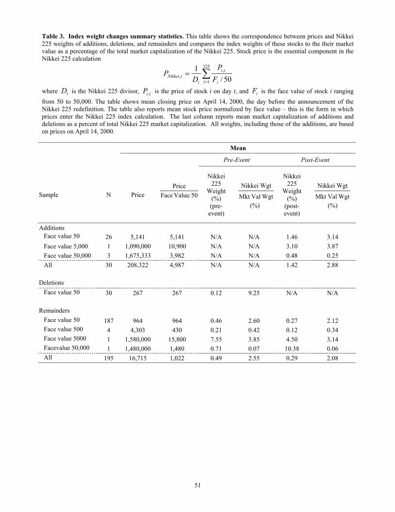
51

Table 3. Index weight changes summary statistics. This table shows the correspondence between prices and Nikkei 225 weights of additions, deletions, and remainders and compares the index weights of these stocks to the their market value as a percentage of the total market capitalization of the Nikkei 225. Stock price is the essential component in the Nikkei 225 calculation

∑=

=225

1

,, 50/

1i i

ti

ttNikkei F

PD

P

where tD is the Nikkei 225 divisor, tiP , is the price of stock i on day t, and iF is the face value of stock i ranging from 50 to 50,000. The table shows mean closing price on April 14, 2000, the day before the announcement of the Nikkei 225 redefinition. The table also reports mean stock price normalized by face value – this is the form in which prices enter the Nikkei 225 index calculation. The last column reports mean market capitalization of additions and deletions as a percent of total Nikkei 225 market capitalization. All weights, including those of the additions, are based on prices on April 14, 2000.

Mean

Pre-Event Post-Event

Sample N Price 50Value FacePrice

Nikkei 225

Weight (%) (pre-

event)

WgtValMkt

WgtNikkei

(%)

Nikkei 225

Weight (%)

(post-event)

WgtValMkt

WgtNikkei

(%)

Additions Face value 50 26 5,141 5,141 N/A N/A 1.46 3.14 Face value 5,000 1 1,090,000 10,900 N/A N/A 3.10 3.87 Face value 50,000 3 1,675,333 3,982 N/A N/A 0.48 0.25 All 30 208,322 4,987 N/A N/A 1.42 2.88 Deletions Face value 50 30 267 267 0.12 9.25 N/A N/A Remainders Face value 50 187 964 964 0.46 2.60 0.27 2.12 Face value 500 4 4,303 430 0.21 0.42 0.12 0.34 Face value 5000 1 1,580,000 15,800 7.55 3.85 4.50 3.14 Facevalue 50,000 1 1,480,000 1,480 0.71 0.07 10.38 0.06 All 195 16,715 1,022 0.49 2.55 0.29 2.08

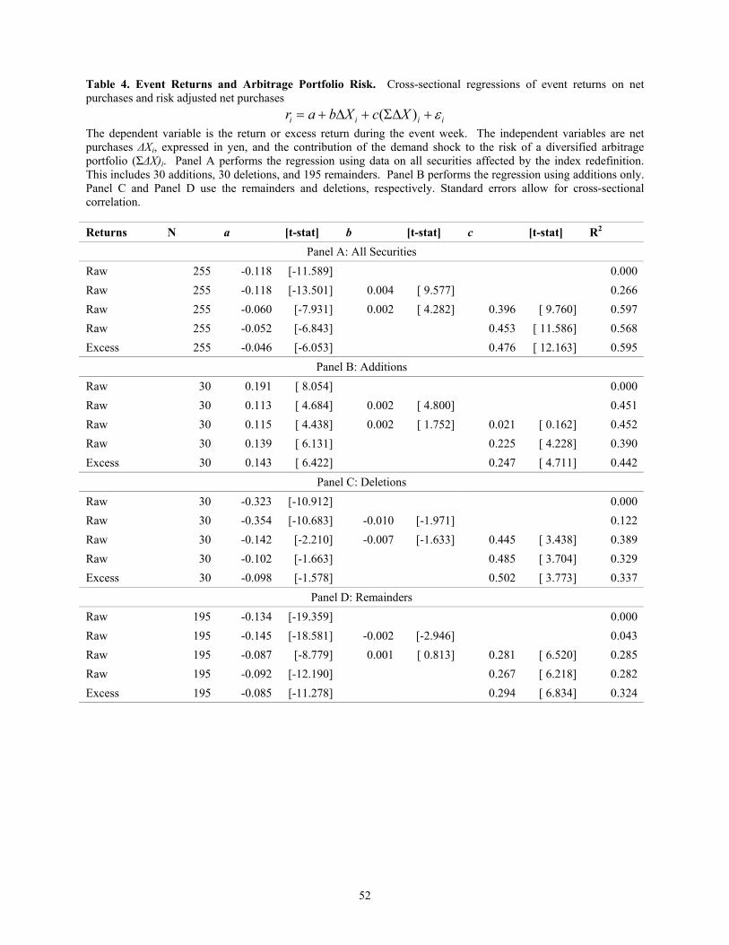
52

Table 4. Event Returns and Arbitrage Portfolio Risk. Cross-sectional regressions of event returns on net purchases and risk adjusted net purchases

iiii XcXbar ε+Σ∆+∆+= )( The dependent variable is the return or excess return during the event week. The independent variables are net purchases ∆Xi, expressed in yen, and the contribution of the demand shock to the risk of a diversified arbitrage portfolio (Σ∆X)i. Panel A performs the regression using data on all securities affected by the index redefinition. This includes 30 additions, 30 deletions, and 195 remainders. Panel B performs the regression using additions only. Panel C and Panel D use the remainders and deletions, respectively. Standard errors allow for cross-sectional correlation. Returns N a [t-stat] b [t-stat] c [t-stat] R2

Panel A: All Securities Raw 255 -0.118 [-11.589] 0.000 Raw 255 -0.118 [-13.501] 0.004 [ 9.577] 0.266 Raw 255 -0.060 [-7.931] 0.002 [ 4.282] 0.396 [ 9.760] 0.597 Raw 255 -0.052 [-6.843] 0.453 [ 11.586] 0.568 Excess 255 -0.046 [-6.053] 0.476 [ 12.163] 0.595

Panel B: Additions Raw 30 0.191 [ 8.054] 0.000 Raw 30 0.113 [ 4.684] 0.002 [ 4.800] 0.451 Raw 30 0.115 [ 4.438] 0.002 [ 1.752] 0.021 [ 0.162] 0.452 Raw 30 0.139 [ 6.131] 0.225 [ 4.228] 0.390 Excess 30 0.143 [ 6.422] 0.247 [ 4.711] 0.442

Panel C: Deletions Raw 30 -0.323 [-10.912] 0.000 Raw 30 -0.354 [-10.683] -0.010 [-1.971] 0.122 Raw 30 -0.142 [-2.210] -0.007 [-1.633] 0.445 [ 3.438] 0.389 Raw 30 -0.102 [-1.663] 0.485 [ 3.704] 0.329 Excess 30 -0.098 [-1.578] 0.502 [ 3.773] 0.337

Panel D: Remainders Raw 195 -0.134 [-19.359] 0.000 Raw 195 -0.145 [-18.581] -0.002 [-2.946] 0.043 Raw 195 -0.087 [-8.779] 0.001 [ 0.813] 0.281 [ 6.520] 0.285 Raw 195 -0.092 [-12.190] 0.267 [ 6.218] 0.282 Excess 195 -0.085 [-11.278] 0.294 [ 6.834] 0.324

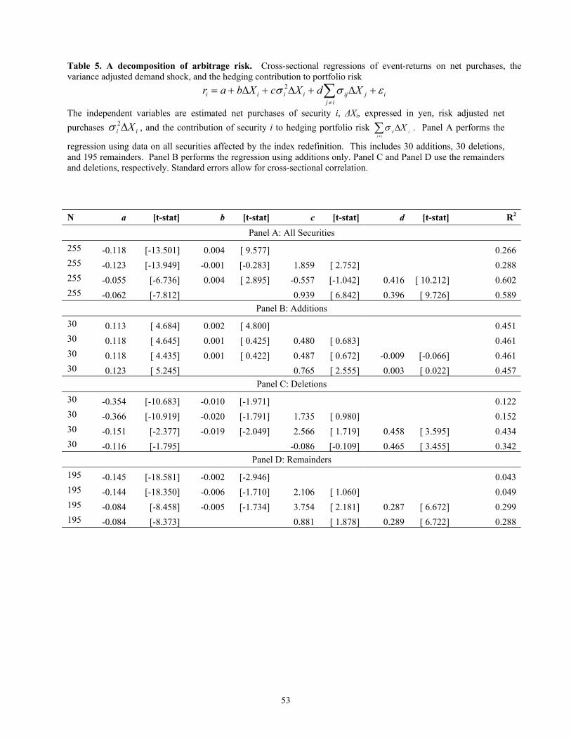
53

Table 5. A decomposition of arbitrage risk. Cross-sectional regressions of event-returns on net purchases, the variance adjusted demand shock, and the hedging contribution to portfolio risk

iij

jijiiii XdXcXbar εσσ +∆+∆+∆+= ∑≠

2

The independent variables are estimated net purchases of security i, ∆Xi, expressed in yen, risk adjusted net purchases ii X∆2σ , and the contribution of security i to hedging portfolio risk ∑

≠

∆ij

jij Xσ . Panel A performs the

regression using data on all securities affected by the index redefinition. This includes 30 additions, 30 deletions, and 195 remainders. Panel B performs the regression using additions only. Panel C and Panel D use the remainders and deletions, respectively. Standard errors allow for cross-sectional correlation.

N a [t-stat] b [t-stat] c [t-stat] d [t-stat] R2

Panel A: All Securities

255 -0.118 [-13.501] 0.004 [ 9.577] 0.266 255 -0.123 [-13.949] -0.001 [-0.283] 1.859 [ 2.752] 0.288 255 -0.055 [-6.736] 0.004 [ 2.895] -0.557 [-1.042] 0.416 [ 10.212] 0.602 255 -0.062 [-7.812] 0.939 [ 6.842] 0.396 [ 9.726] 0.589

Panel B: Additions

30 0.113 [ 4.684] 0.002 [ 4.800] 0.451 30 0.118 [ 4.645] 0.001 [ 0.425] 0.480 [ 0.683] 0.461 30 0.118 [ 4.435] 0.001 [ 0.422] 0.487 [ 0.672] -0.009 [-0.066] 0.461 30 0.123 [ 5.245] 0.765 [ 2.555] 0.003 [ 0.022] 0.457

Panel C: Deletions

30 -0.354 [-10.683] -0.010 [-1.971] 0.122 30 -0.366 [-10.919] -0.020 [-1.791] 1.735 [ 0.980] 0.152 30 -0.151 [-2.377] -0.019 [-2.049] 2.566 [ 1.719] 0.458 [ 3.595] 0.434 30 -0.116 [-1.795] -0.086 [-0.109] 0.465 [ 3.455] 0.342

Panel D: Remainders

195 -0.145 [-18.581] -0.002 [-2.946] 0.043 195 -0.144 [-18.350] -0.006 [-1.710] 2.106 [ 1.060] 0.049 195 -0.084 [-8.458] -0.005 [-1.734] 3.754 [ 2.181] 0.287 [ 6.672] 0.299 195 -0.084 [-8.373] 0.881 [ 1.878] 0.289 [ 6.722] 0.288

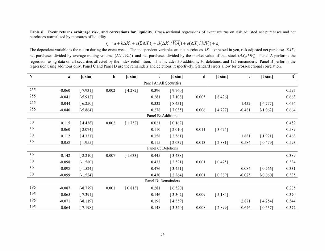
54

Table 6. Event returns arbitrage risk, and corrections for liquidity. Cross-sectional regressions of event returns on risk adjusted net purchases and net purchases normalized by measures of liquidity

iiiiiiii MVXeVolXdXcXbar ε+∆+∆+Σ∆+∆+= )/()/()( The dependent variable is the return during the event week. The independent variables are net purchases ∆Xi, expressed in yen, risk adjusted net purchases Σ∆Xi, net purchases divided by average trading volume )/( ii VolX∆ and net purchases divided by the market value of that stock (∆Xi,/MVi). Panel A performs the regression using data on all securities affected by the index redefinition. This includes 30 additions, 30 deletions, and 195 remainders. Panel B performs the regression using additions only. Panel C and Panel D use the remainders and deletions, respectively. Standard errors allow for cross-sectional correlation. N a [t-stat] b [t-stat] c [t-stat] d [t-stat] e [t-stat] R2

Panel A: All Securities 255 -0.060 [-7.931] 0.002 [ 4.282] 0.396 [ 9.760] 0.597 255 -0.041 [-5.912] 0.281 [ 7.108] 0.005 [ 8.426] 0.663 255 -0.044 [-6.250] 0.332 [ 8.431] 1.432 [ 6.777] 0.634 255 -0.040 [-5.864] 0.278 [ 7.035] 0.006 [ 4.727] -0.481 [-1.062] 0.664

Panel B: Additions 30 0.115 [ 4.438] 0.002 [ 1.752] 0.021 [ 0.162] 0.452 30 0.060 [ 2.074] 0.110 [ 2.010] 0.011 [ 3.624] 0.589 30 0.112 [ 4.331] 0.158 [ 2.561] 1.881 [ 1.921] 0.463 30 0.058 [ 1.955] 0.115 [ 2.037] 0.013 [ 2.881] -0.584 [-0.479] 0.593

Panel C: Deletions 30 -0.142 [-2.210] -0.007 [-1.633] 0.445 [ 3.438] 0.389 30 -0.098 [-1.580] 0.433 [ 2.521] 0.001 [ 0.475] 0.334 30 -0.098 [-1.524] 0.476 [ 3.451] 0.084 [ 0.266] 0.331 30 -0.099 [-1.524] 0.430 [ 2.364] 0.001 [ 0.389] -0.025 [-0.060] 0.335

Panel D: Remainders 195 -0.087 [-8.779] 0.001 [ 0.813] 0.281 [ 6.520] 0.285 195 -0.065 [-7.391] 0.146 [ 3.302] 0.009 [ 5.184] 0.370 195 -0.071 [-8.119] 0.198 [ 4.559] 2.871 [ 4.254] 0.344 195 -0.064 [-7.198] 0.148 [ 3.340] 0.008 [ 2.899] 0.646 [ 0.637] 0.372

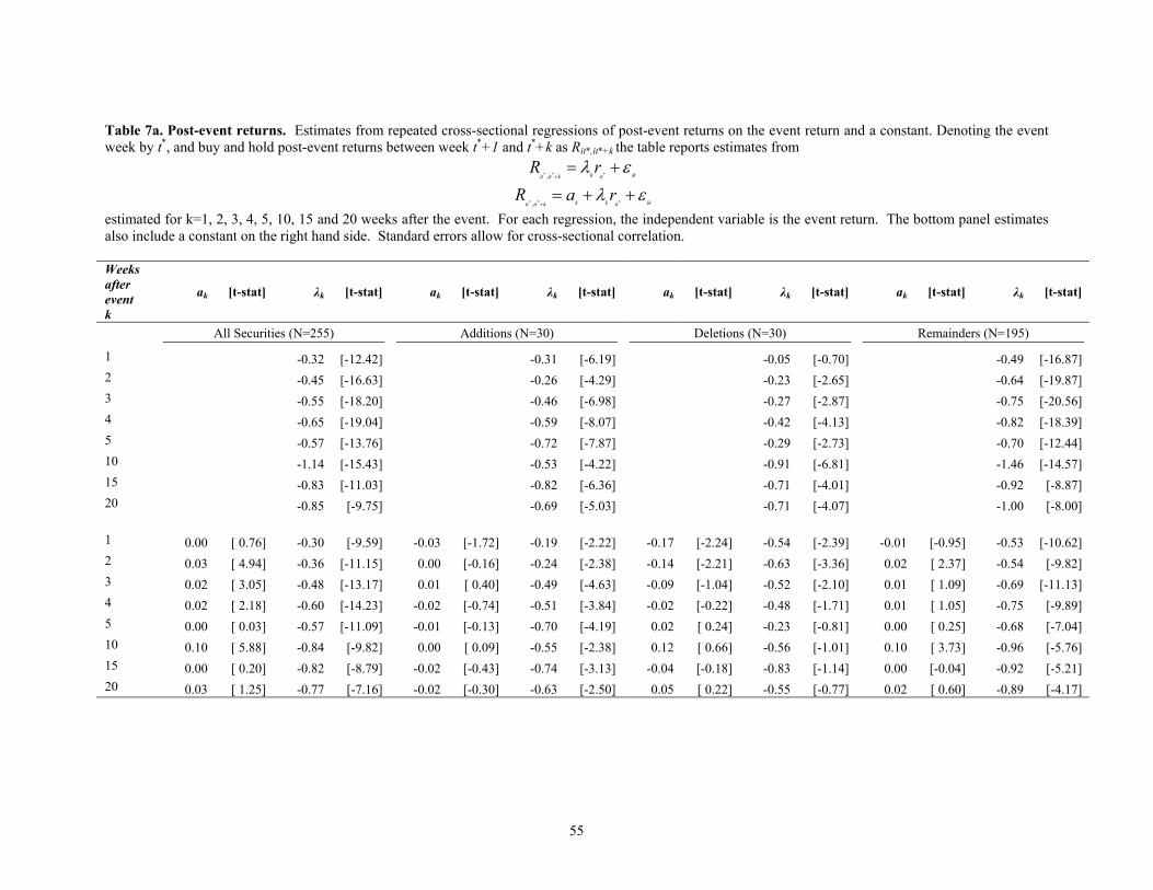
55

Table 7a. Post-event returns. Estimates from repeated cross-sectional regressions of post-event returns on the event return and a constant. Denoting the event week by t*, and buy and hold post-event returns between week t*+1 and t*+k as Rit*,it*+k the table reports estimates from

ikitkkititrR ελ +=

+ *** ,

ikitkkkitit

raR ελ ++=+ *** ,

estimated for k=1, 2, 3, 4, 5, 10, 15 and 20 weeks after the event. For each regression, the independent variable is the event return. The bottom panel estimates also include a constant on the right hand side. Standard errors allow for cross-sectional correlation. Weeks after event k

ak

[t-stat] λk [t-stat] ak

[t-stat] λk [t-stat] ak

[t-stat] λk [t-stat] ak

[t-stat] λk [t-stat]

All Securities (N=255) Additions (N=30) Deletions (N=30) Remainders (N=195)

1 -0.32 [-12.42] -0.31 [-6.19] -0.05 [-0.70] -0.49 [-16.87] 2 -0.45 [-16.63] -0.26 [-4.29] -0.23 [-2.65] -0.64 [-19.87] 3 -0.55 [-18.20] -0.46 [-6.98] -0.27 [-2.87] -0.75 [-20.56] 4 -0.65 [-19.04] -0.59 [-8.07] -0.42 [-4.13] -0.82 [-18.39] 5 -0.57 [-13.76] -0.72 [-7.87] -0.29 [-2.73] -0.70 [-12.44] 10 -1.14 [-15.43] -0.53 [-4.22] -0.91 [-6.81] -1.46 [-14.57] 15 -0.83 [-11.03] -0.82 [-6.36] -0.71 [-4.01] -0.92 [-8.87] 20 -0.85 [-9.75] -0.69 [-5.03] -0.71 [-4.07] -1.00 [-8.00] 1 0.00 [ 0.76] -0.30 [-9.59] -0.03 [-1.72] -0.19 [-2.22] -0.17 [-2.24] -0.54 [-2.39] -0.01 [-0.95] -0.53 [-10.62] 2 0.03 [ 4.94] -0.36 [-11.15] 0.00 [-0.16] -0.24 [-2.38] -0.14 [-2.21] -0.63 [-3.36] 0.02 [ 2.37] -0.54 [-9.82] 3 0.02 [ 3.05] -0.48 [-13.17] 0.01 [ 0.40] -0.49 [-4.63] -0.09 [-1.04] -0.52 [-2.10] 0.01 [ 1.09] -0.69 [-11.13] 4 0.02 [ 2.18] -0.60 [-14.23] -0.02 [-0.74] -0.51 [-3.84] -0.02 [-0.22] -0.48 [-1.71] 0.01 [ 1.05] -0.75 [-9.89] 5 0.00 [ 0.03] -0.57 [-11.09] -0.01 [-0.13] -0.70 [-4.19] 0.02 [ 0.24] -0.23 [-0.81] 0.00 [ 0.25] -0.68 [-7.04] 10 0.10 [ 5.88] -0.84 [-9.82] 0.00 [ 0.09] -0.55 [-2.38] 0.12 [ 0.66] -0.56 [-1.01] 0.10 [ 3.73] -0.96 [-5.76] 15 0.00 [ 0.20] -0.82 [-8.79] -0.02 [-0.43] -0.74 [-3.13] -0.04 [-0.18] -0.83 [-1.14] 0.00 [-0.04] -0.92 [-5.21] 20 0.03 [ 1.25] -0.77 [-7.16] -0.02 [-0.30] -0.63 [-2.50] 0.05 [ 0.22] -0.55 [-0.77] 0.02 [ 0.60] -0.89 [-4.17]

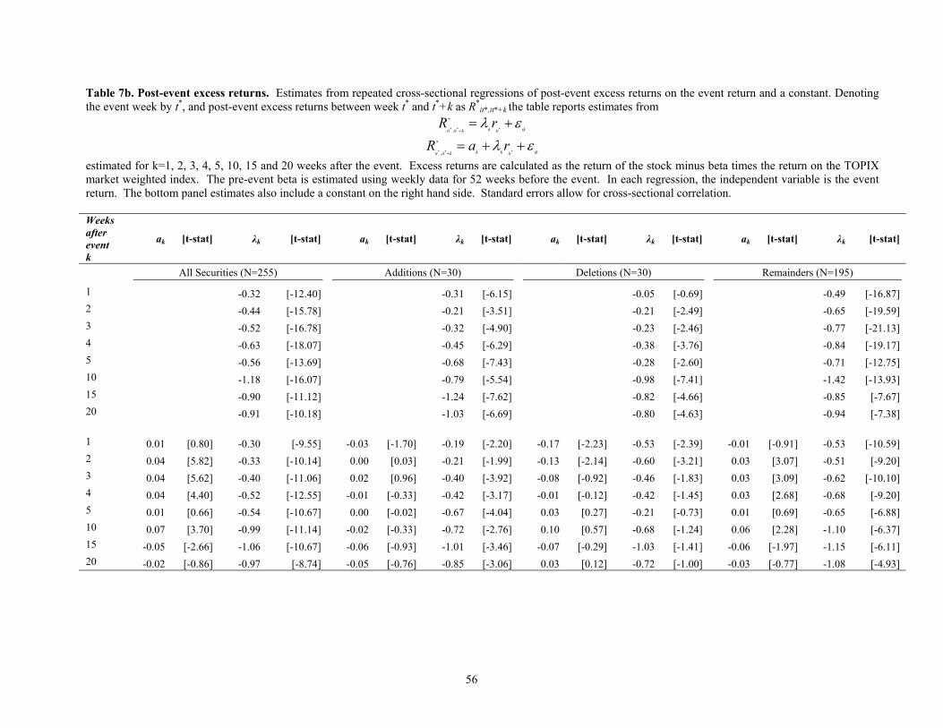
56

Table 7b. Post-event excess returns. Estimates from repeated cross-sectional regressions of post-event excess returns on the event return and a constant. Denoting the event week by t*, and post-event excess returns between week t* and t*+k as R*

it*,it*+k the table reports estimates from

ikitkkititrR ελ +=

+ ***

*

,

ikitkkkitit

raR ελ ++=+ ***

*

,

estimated for k=1, 2, 3, 4, 5, 10, 15 and 20 weeks after the event. Excess returns are calculated as the return of the stock minus beta times the return on the TOPIX market weighted index. The pre-event beta is estimated using weekly data for 52 weeks before the event. In each regression, the independent variable is the event return. The bottom panel estimates also include a constant on the right hand side. Standard errors allow for cross-sectional correlation. Weeks after event k

ak

[t-stat] λk [t-stat] ak

[t-stat] λk [t-stat] ak

[t-stat] λk [t-stat] ak

[t-stat] λk [t-stat]

All Securities (N=255) Additions (N=30) Deletions (N=30) Remainders (N=195)

1 -0.32 [-12.40] -0.31 [-6.15] -0.05 [-0.69] -0.49 [-16.87] 2 -0.44 [-15.78] -0.21 [-3.51] -0.21 [-2.49] -0.65 [-19.59] 3 -0.52 [-16.78] -0.32 [-4.90] -0.23 [-2.46] -0.77 [-21.13] 4 -0.63 [-18.07] -0.45 [-6.29] -0.38 [-3.76] -0.84 [-19.17] 5 -0.56 [-13.69] -0.68 [-7.43] -0.28 [-2.60] -0.71 [-12.75] 10 -1.18 [-16.07] -0.79 [-5.54] -0.98 [-7.41] -1.42 [-13.93] 15 -0.90 [-11.12] -1.24 [-7.62] -0.82 [-4.66] -0.85 [-7.67] 20 -0.91 [-10.18] -1.03 [-6.69] -0.80 [-4.63] -0.94 [-7.38] 1 0.01 [0.80] -0.30 [-9.55] -0.03 [-1.70] -0.19 [-2.20] -0.17 [-2.23] -0.53 [-2.39] -0.01 [-0.91] -0.53 [-10.59] 2 0.04 [5.82] -0.33 [-10.14] 0.00 [0.03] -0.21 [-1.99] -0.13 [-2.14] -0.60 [-3.21] 0.03 [3.07] -0.51 [-9.20] 3 0.04 [5.62] -0.40 [-11.06] 0.02 [0.96] -0.40 [-3.92] -0.08 [-0.92] -0.46 [-1.83] 0.03 [3.09] -0.62 [-10.10] 4 0.04 [4.40] -0.52 [-12.55] -0.01 [-0.33] -0.42 [-3.17] -0.01 [-0.12] -0.42 [-1.45] 0.03 [2.68] -0.68 [-9.20] 5 0.01 [0.66] -0.54 [-10.67] 0.00 [-0.02] -0.67 [-4.04] 0.03 [0.27] -0.21 [-0.73] 0.01 [0.69] -0.65 [-6.88] 10 0.07 [3.70] -0.99 [-11.14] -0.02 [-0.33] -0.72 [-2.76] 0.10 [0.57] -0.68 [-1.24] 0.06 [2.28] -1.10 [-6.37] 15 -0.05 [-2.66] -1.06 [-10.67] -0.06 [-0.93] -1.01 [-3.46] -0.07 [-0.29] -1.03 [-1.41] -0.06 [-1.97] -1.15 [-6.11] 20 -0.02 [-0.86] -0.97 [-8.74] -0.05 [-0.76] -0.85 [-3.06] 0.03 [0.12] -0.72 [-1.00] -0.03 [-0.77] -1.08 [-4.93]