SHOCKS AND THE SPATIAL DISTRIBUTION OF ECONOMIC

ACTIVITY: THE ROLE OF INSTITUTIONS

Patrick A. Testa∗

October 22, 2020

Abstract

Why do some historical shocks permanently impact local development, while othersdo not? This paper examines how institutions influence local recovery to populationshocks, using a model with multiple regions and increasing returns to economic activitywithin regions. Extractive institutions crowd out productive activity, making its spatialcoordination more difficult in the aftermath of large, negative shocks. Hence, when oneregion experiences such a shock, extractive institutions can hinder recovery, ensuring aredistribution of productive activity away from that region over the long-run. Using adataset of major earthquakes and 1860 world cities from 1973 to 2018, I find sustainednegative effects of earthquakes on city population growth, with effects being driven bycities located outside of stable democracies, consistent with the theory.

JEL codes: B52, C72, J24, P48, R12Key words: History dependence; multiple equilibria; institutions; increasing returns; earth-quakes

∗Department of Economics, 6823 St. Charles Avenue, Tulane University, New Orleans, LA 70118, UnitedStates of America. Email: ptesta@tulane.edu. Phone: +1 (507) 261-7728. I am grateful to the editors, MarkKoyama and Daniel Houser, as well as two anonymous referees for comments that substantially improvedthis paper. The paper also greatly benefited from discussions with and feedback from Dan Bogart, Jean-PaulCarvalho, Areendam Chanda, Matthew Freedman, Dan Keniston, Igor Kopylov, Adam Meirowitz, MichaelShin, Stergios Skaperdas, and Cole Randall Williams, as well as seminar participants at UC Irvine, Tulane,LSU, George Mason, and Alberta. All errors are my own. Declarations of interest: none.

1 Introduction

In 2010, a 7.0 magnitude earthquake struck just outside of Port-au-Prince, Haiti. In the

years following, the city witnessed a nearly 50% decline in annual population growth, a

trend which has persisted ever since.1 A year later and across the world, an even larger

earthquake struck off the coast of Sendai, Japan, fueling massive tsunamis. Today, that city

is enjoying its highest levels of population growth in over a decade.2

Why do some historical shocks permanently impact local development, while others do

not? And what factors determine the distribution of economic activity across space more

generally? These questions are of central importance in urban and development economics for

understanding differences in economic performance within countries, as well as the potential

role of policy. Despite this, their answers remain subject to active debate.

One theory is that there exists the potential for multiple equilibria in spatial development

but conditions set by both nature and history select among them. In this view, the location

of economic activity is driven in part by incentives for humans to locate near each other, such

as in production (i.e. agglomeration spillovers). Such increasing returns can generate path

dependence, while also implying a potential for policy to induce or transplant economic ac-

tivity in self-reinforcing ways (Kline and Moretti, 2014; Jedwab and Moradi, 2016). However,

some empirical research has cast doubt upon the empirical relevance of multiple equilibria.

Davis and Weinstein (2002, 2008) and Miguel and Roland (2011), among others, have shown

how even massive shocks may only temporarily redistribute economic activity across space.

This literature supports a more deterministic view, in which individuals co-gravitate toward

strong fundamentals over the long-run, while returns to scale matter more for determining

spatial dispersion (e.g. of cities). Efforts to reconcile these findings have varied considerably,

with selection in shock exposure, focal points, and heterogeneity in physical geography all

being proposed as potential sources of differential effects (Redding, 2010; Acemoglu, Hassan,

and Robinson, 2011; Bleakley and Lin, 2012; Nunn, 2009, 2014; Schumann, 2014; Jedwab,

Johnson, and Koyama, 2019).3

This paper provides an alternative approach to understanding this empirical puzzle, by

considering the interaction of increasing returns with another important force for long-run

development: formal institutions (Acemoglu, Johnson, and Robinson, 2001; Dell, 2010; Ace-

moglu and Dell, 2010). Using a two-region model with migration between regions, I explore

1In 2009, Port-au-Prince added approximately 126,712 to its population; in 2018, it added only 67,782.2Between 2017 and 2018, Sendai grew by approximately 18,131, its largest increase since 2005 saw 20,960.3In addition, an alternative theory for the persistence of shocks posits that growth follows a random walk

(Simon, 1955; Gabaix, 1999). While I do not focus on this mechanism in this paper, I do discuss and providesome evidence against it in the context of the empirical exercise in Section 3.

1

the role of institutions in explaining the differential impact of temporary shocks on the

long-run spatial distribution of economic activity. In the model, more extractive institutions

decrease the return on production relative to “unproductive” activities that do not contribute

to the productive process, thus utilizing resources at the expense of it (Nunn, 2007). In the

presence of increasing returns to productive activity within regions, a large negative shock

to a region’s population can temporarily reduce productive spillovers. When institutions are

sufficiently extractive, this can induce substitution among workers from productive into un-

productive activities. Now absent productive spillovers, relatively fewer workers will prefer

to live in the affected region, while those who do migrate there will also prefer to engage in

unproductive activities, locking in asymmetries in both population and production between

regions.

Hence, the model exhibits multiple equilibria: one with two similarly productive and

populated regions, and one with a single highly populated, productive region neighboring a

less populated and relatively unproductive region. Moreover, these asymmetries can arise

even when there are no differences in natural advantages, local institutions, or endowments

ex ante between regions. Then, as institutions become stronger and less extractive, spatial

equilibria become more robust to large shocks. This illustrates how relatively lowered levels

of economic activity may persist in a region following a negative population shock, causing

population and productive inputs such as human capital to become concentrated in select

regions over the long-run – even if formal institutions eventually improve.

The notion that institutions can have long-lasting effects on economic development is

not new. A large theoretical and empirical literature exists documenting numerous cases

throughout history in which extraction negatively impacted long-run development. Human

capital (Acemoglu, Gallego, and Robinson, 2014), culture (Tabellini, 2010), and public goods

provision (Dell, 2010) have all been cited as important channels through which historical

institutions continue to matter. Most similar to this paper is Nunn (2007), who models a

similar tradeoff between productive and unproductive activities in explaining the importance

of historical extraction. This paper goes a step further, exploring how national institutions

influence the persistence of shocks, and therefore the distribution of economic activity, within

countries. In particular, it argues that in places that feature less economic activity, extractive

institutions promote comparative advantages in unproductive activities that, as such, do not

attract productive workers. In the context of a large shock, such as a natural disaster, this

means that activities such as corruption and property theft made more attractive by weak

institutions are present to reinforce the effects of the initial shock. It also means that, by

weakening incentives underlying urban recovery in the short-run, weak central institutions

may produce greater variation in development within countries.

2

Nevertheless, a link between the institutional environment experienced by a country or

region and the persistence of population shocks therein has often been alluded to in existing

empirical research on war, expulsion, and natural disaster. Mirroring Davis and Weinstein’s

(2002, 2008) finding that Japanese city size and composition were robust to the bombings

of WWII, returning to their prewar distributions within decades, Miguel and Roland (2011)

observe similar convergence in Vietnam. At the same time, they argue that differential

convergence would be unsurprising in a larger sample of studies. In particular, the authors

note that while postwar Japan was a market democracy and Vietnam a socialist regime, both

had relatively strong institutions, which would have aided in catch-up in both places. Similar

points about the importance of preexisting institutions are made by Brakman, Garretsen,

and Schramm (2004), who find swift convergence after WWII in West but not East Germany,

as well as in surveys of the empirical literature by Redding (2010) and Nunn (2014).

Given this, it is perhaps unsurprising that much of the work on forced migration has

shown, in contrast, strong persistence in the origin economy. For instance, Chaney and

Hornbeck (2016) find delayed convergence following the expulsion of Moriscos from Spain in

1609, citing preexisting extractive institutions in Morisco areas as a potential source. Testa

(2020) similarly finds Czech municipalities affected by expulsions of Germans after WWII to

be worse off today relative to unaffected areas nearby, attributing these differences in part to

the widespread property exploitation that took place of affected areas by settlers and local

officials. Meanwhile, Nunn (2008) finds a negative relationship between exports of slaves

and future economic performance in African countries, characterizing the slave trade as an

extractive regime that gave rise to raiding and internal warfare in origin economies.

Such can also be found in the relatively smaller literature on non-political population

shocks, such as natural disaster. In the case of earthquakes, Barone and Mocetti (2014)

cite preexisting institutions as a source of differential effects, with corruption and declining

social capital impeding recovery in poorly institutionalized places, while Anbarci, Escaleras,

and Register (2005) similarly show poor collective action to exacerbate earthquake fatali-

ties in places with greater inequality, and Belloc, Drago, and Galbiati (2016) observe local

institutional stagnation following earthquakes in medieval Italy in places where separation

of relevant powers had previously been weak. Meanwhile, Acemoglu, de Feo, and de Luca

(2019) find that severe droughts paved the way for the Sicilian Mafia where institutions were

weak, at the expense of subsequent local development.4

4Also see Maloney and Caicedo (2015) and Jedwab, Johnson, and Koyama (2019) for more on institutionsas a source of heterogeneous effects in the persistence of pre-colonial American agglomerations and the BlackDeath, respectively, as well as Dell and Olken (2019) for evidence that within the extractive colonial Dutchregime in Java, agglomeration economies from sugar factories gave rise to countervailing long-run effectslocally.

3

The remainder of the paper adds to this empirical literature by testing the predictions

of the model. To do this, I consider the effects of large earthquakes on city population

growth over time, using a dataset of all major earthquakes (i.e. 5 or greater magnitude on

the Richter scale) and population size for 1860 world cities from 1973 to 2018. I first show

that earthquakes tend to have a negative impact on city population growth, with this effect

becoming large and growing over time when I account for a city’s time-invariant earthquake

risk. When I examine heterogeneous effects on the basis of political institutions, I find this

effect to be driven by cities located outside of stable democracies, in line with the predictions

of the model. These findings complement an existing literature on the economic effects of

earthquakes and other national disasters, to which they contribute an examination into the

city-level population effects of earthquakes at a global level (Ahlerup, 2013; Cavallo et al,

2013; Hsiang and Jina, 2014; Boustan et al, 2017; Kirchberger, 2017).5

2 The model

The economy in the model is composed of a share of non-atomic workers Mr in each region

r ∈ {1, 2}. Workers are long-lived but myopic, and I focus for now on a single time period.

Each worker begins a period with some endowment, which she may choose to transform into

a labor input, h (e.g. human capital). If she does, then her labor input is combined with a

firm’s resources to produce goods, and she is compensated at the regional market wage rate

wr. In this scenario, she is said to be engaged in production. At any given time, the share

of all workers living in region r and engaged in production is mr ≤ Mr.6 Each region also

has a fixed stock of resources, K, which are divided amongst λ ∗ mr identically-producing

firms indexed by ω.7 In a given period, each region r firm has some amount kr ≤ K/λmr of

resources for use in production, to be defined shortly.

However, a worker may also choose to forgo engagement in production. In this scenario,

she simply consumes resources directly – resources which might otherwise be used by firms as

inputs in production. I refer to such behavior as unproductive, to the extent that it does not

contribute to the local production process and as such comes at its expense. The relative

payoffs from unproductive activities as compared to productive ones crucially depend on

the formal institutional environment. The assumption that extractive or weak institutions

decrease the relative payoffs from productive activities and give rise to unproductive behavior

is long-standing in the political economy literature (Skaperdas, 1992; Nunn, 2007). In this

5A more similar empirical study is Kocornik-Mina (2019), who find persistent urban effects of floods.6Thus the share of the world’s workforce that is engaged in production is mr + m−r ≤ 1, where the

prevalence of productive worker activity in region r does not necessarily scale with but is constrained by Mr.7For simplicity, K is immobile and regenerates each period.

4

model, the quality of institutions is exogenous to local economic activity and represented

simply by the parameter β.8

The productive environment

Production is subject to constant returns to scale within firms in resources and labor inputs.

However, the model allows for external increasing returns (i.e. within regions) in regional

labor inputs Hr ≡ mrh. In this case, as relatively more productive activity locates in region

r, region r firms can produce relatively more given the same labor inputs. This agglomeration

spillover is represented by Hγr , where γ ≥ 0 gives its magnitude.9

Besides agglomeration, heterogeneity across regions in firm-level productivity can also be

attributed to differences in natural advantages. These locational benefits are given by the

parameter ar. Thus the overall productivity level for region r is given by:

Ar = arHγr .

Altogether, this yields a firm-level CRS production function of:

fr(ω) = Arkrhr(ω),

where hr(ω) gives a region r firm’s demand for labor inputs. Hence, a firm’s profit maxi-

mization problem can be given by:

maxhr(ω)

parHγr krhr(ω)− wrhr(ω), (1)

where prices p are set collectively by all regions with workers engaged in production.10

Assuming zero profit, this implies a real income and thus consumption payoffs for productive

8This assumption implies that, as a measure of central institutions, β is invariant to the local economicconditions within individual regions. As the model shows, however, the implications of poor central insti-tutions may nonetheless vary by region, with some regions being as if they are in a country with goodinstitutions, making the effective institutional environment endogenous within regions. Complicating themodel so β is instead modeled as endogenous to local economic activity simply magnifies existing strategiccomplementaries in local worker behavior, as shown in Theory Discussion 1 in the Supplemental Material.

9This term is common in the economic geography literature (Allen and Donaldson, 2018). For microfoun-dations, see Marshall (1920) and Duranton and Puga (2004). For empirical estimation, see Rosenthal andStrange (2004), Moretti (2004), Greenstone, Hornbeck, and Moretti (2010), and Ellison, Glaeser, and Kerr(2010).

10As regions are in close proximity, I assume no trade costs or differences in market access.

5

workers in region r of:

Vr(h) = arHγr kr ∗ h

= arkrh1+γmγ

r .(2)

How does the institutional environment matter?

Unlike typical two-region models of economic geography, this framework incorporates a

strategic component in which workers may prefer to engage in unproductive activities. In

contrast with production, which involves combining worker endowments with resources to

create value for consumers, unproductive activities involve acquiring and consuming re-

sources directly (i.e. every man for himself), which does not entail external economies of

scale, while coming at the expense of the local productive sector, which does. This distinction

between productive and unproductive activities is common in the literature on institutions

and conflict (Acemoglu, 1995; Nunn, 2007). Real-world examples of unproductive activities

include corruption and rent-seeking, as well as looting and other property crime. Institu-

tional qualities that might drive relatively high payoffs from such activities, e.g. following a

negative shock such as a bombing or natural disaster, include poor property rights protection

and weak rule of law in the enforcement of building codes and aid dispersal.

I model such resource acquisition using a variant of the contest success function (Skaper-

das, 1996). Unproductive workers consume resources that would otherwise be used in pro-

duction, where the total amount of resources acquired by unproductive workers in region r

is proportional to the relative prevalence of unproductive behavior in the regional economy:

Mr −mr

Mr

K,

where Mr−mr equals the share of all workers living in region r and engaged in unproductive

activities. This leaves each region r firm with a final resource endowment of:

k∗r =

(1− Mr −mr

Mr

)K

λmr

=K

λMr

.

(3)

Unproductive payoffs follow from this. Adopting the assumption that relative value from

unproductive activities is derived inversely from the quality of institutions, consider the

6

following payoffs from engaging in unproductive activities in region r:

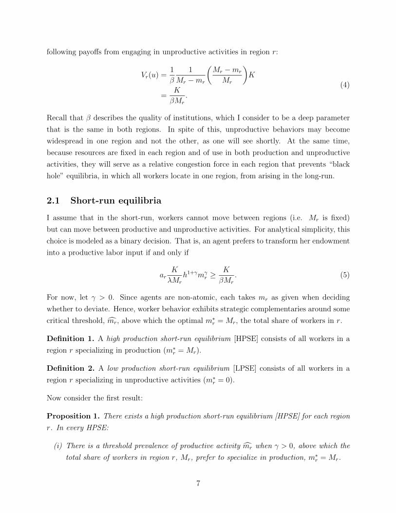
Vr(u) =1

β

1

Mr −mr

(Mr −mr

Mr

)K

=K

βMr

.

(4)

Recall that β describes the quality of institutions, which I consider to be a deep parameter

that is the same in both regions. In spite of this, unproductive behaviors may become

widespread in one region and not the other, as one will see shortly. At the same time,

because resources are fixed in each region and of use in both production and unproductive

activities, they will serve as a relative congestion force in each region that prevents “black

hole” equilibria, in which all workers locate in one region, from arising in the long-run.

2.1 Short-run equilibria

I assume that in the short-run, workers cannot move between regions (i.e. Mr is fixed)

but can move between productive and unproductive activities. For analytical simplicity, this

choice is modeled as a binary decision. That is, an agent prefers to transform her endowment

into a productive labor input if and only if

arK

λMr

h1+γmγr ≥

K

βMr

. (5)

For now, let γ > 0. Since agents are non-atomic, each takes mr as given when deciding

whether to deviate. Hence, worker behavior exhibits strategic complementaries around some

critical threshold, mr, above which the optimal m∗r = Mr, the total share of workers in r.

Definition 1. A high production short-run equilibrium [HPSE] consists of all workers in a

region r specializing in production (m∗r = Mr).

Definition 2. A low production short-run equilibrium [LPSE] consists of all workers in a

region r specializing in unproductive activities (m∗r = 0).

Now consider the first result:

Proposition 1. There exists a high production short-run equilibrium [HPSE] for each region

r. In every HPSE:

(i) There is a threshold prevalence of productive activity mr when γ > 0, above which the

total share of workers in region r, Mr, prefer to specialize in production, m∗r = Mr.

7

(ii) The share of the worker population located in r must be sufficiently large, Mr ≥ mr,

where this equilibrium is locally stable in Mr whenever this inequality is strict.

(iii) mr is decreasing in ar, h, and β and increasing in λ.

The remaining space below mr is characterized by a LPSE, in which all agents in region

r forgo production and instead simply acquire and consume local resources (i.e. m∗r = 0).

Importantly, because productive activity entails within-region externalities, and because

the relative prevalence of productive activity in one region is constrained by its relative

population size, a temporary decrease (i.e. shock) in the share of the population located in

that region has the potential to permanently shift it from a HPSE to a LPSE (i.e. Mr < mr

implies mr < mr). However, this depends on the quality of formal institutions. When the

quality of institutions β is sufficiently high, even large shocks will not generate incentives for

workers to substitute toward unproductive activities in the affected region. This is important,

as a population shock which cannot induce a shift from one short-run equilibrium to another

within a region will also have no effect on the long-run equilibrium population distribution

across regions, as we will see shortly.

Now let γ = 0, such that there are no agglomeration spillovers. This is relevant for

understanding how sectors such as agriculture respond to population shocks in the short-

run. As it turns out, population shocks cannot shift a region from one short-run equilibrium

to another in the absence of agglomeration spillovers:

Remark 1. In the absence of agglomeration spillovers, γ = 0, if a HPSE exists in region r

for some Mr, then it exists for all M ′r.

Hence, the propensity for a population shock to shift a regional economy from a HPSE to

a LPSE depends not only on the quality of formal institutions but also on the presence

of external increasing returns (i.e. γ > 0), which generate strategic complementarities in

production choices within regions. In fact, absent agglomeration spillovers, economic activity

will always tend toward its initial distribution as determined by fundamentals regardless of

institutions. To show this, however, I must first introduce population dynamics, in the form

of migration between regions over time.

2.2 Long-run equilibria

In the long-run, agents can move between productive and unproductive activities within

regions as well as migrate between regions. Population dynamics are modeled as in the

8

economic geography literature,11 using a standard replicator dynamic:

Mr = Mr(Vr − V ), (6)

where Mr gives the change over time in the share of the population in region r, which depends

on the relative size of the short-run payoffs in region r, and where V ≡ M1V1 + M2V2 gives

the national average payoffs. There is no cost to migration. However, since agents are non-

atomic, short- and long-run incentives can interact to generate coordination problems which

in turn constrain migration.

Suppose, for instance, that mr ≥ mr initially in each region r, such that both regions

specialize in production (i.e. m∗r = Mr for all r). Then there exists some steady state

Mr ≡ M∗r at which Mr = 0 as long as M∗

r ≥ mr for each region r. That is, when enough

agents are coordinating on productive behavior in each region, mr ≥ mr, there is some

population distribution Mr at which both regions have high levels of production and no

worker prefers to deviate from one region to other. From (2) and (6), this is the solution to:

a1Kh1+γ

λMγ−1

1 =a2Kh

1+γ

λMγ−1

2 , (7)

which implies for each region r:

M∗r =

a1

1−γr

a1

1−γr + a

11−γ−r

.

However, the local stability of this as a long-run equilibrium depends on γ.

Assume for now that γ ∈ (0, 1). When γ ∈ (0, 1), the lefthand side of (7) is strictly

decreasing in Mr while the righthand side is strictly increasing. Then small changes in Mr

will have only temporary effects, holding short-run equilibria fixed. However, by Proposition

1, the stability of this state also depends on the size of Mr relative to the threshold mr for

each region, i.e. local stability in the short-run. I thus define the following:

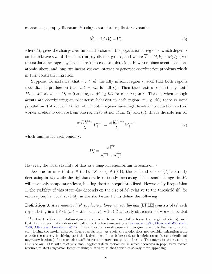
Definition 3. A symmetric high production long-run equilibrium [HPLE] consists of (i) each

region being in a HPSE (m∗r = Mr for all r), with (ii) a steady state share of workers located

11In this tradition, population dynamics are often framed in relative terms (i.e. regional shares), suchthat the total population does not matter for the long-run analysis (Krugman, 1991; Davis and Weinstein,2008; Allen and Donaldson, 2018). This allows for overall population to grow due to births, immigration,etc., letting the model abstract from such factors. As such, the model does not consider migration fromoutside the country in driving post-shock dynamics. That being said, such might occur (absent significantmigratory frictions) if post-shock payoffs in region r grow enough to induce it. This might be the case in anLPSE or an HPSE with relatively small agglomeration economies, in which decreases in population reduceresource-related congestion forces, making migration to that region relatively more appealing.

9

1M∗2M∗∗

2m2 1− m1

M2

M2

Figure 1: Symmetric high production (in blue) versus asymmetric (in red) long-run equilibria for

γ = 1/2, β = 10/3, a1 = a2 = K = h = λ = 1

in each region, M∗r , which is said to be locally stable in Mr if short-run equilibria are locally

stable in Mr (M∗r > mr) and small changes in Mr are temporary (∂Mr

∂Mr|Mr=M∗

r< 0).

Now suppose that Mr and mr are sufficiently close. Then a large, negative shock to Mr in

the short-run (e.g. from death or displacement) may result in a shift to a LPSE in region r,

such that the steady state population distribution is no longer determined by (7).

This brings me to a second case, in which a large, negative shock to e.g. M2 occurs,

shifting region 2 from a HPSE to a LPSE. In other words, in depleting region 2 of its

productive workforce relative to region 1, a large negative population shock reduces its

productive spillovers, thus making it relatively more appealing for those living in region

2 to engage in unproductive behavior, so long as institutions are sufficiently extractive.

Furthermore, conditional upon engaging in unproductive activities, it also increases the

consumable amount of resources per capita in region 2. In the long-run, this will trigger

migration into region 2 by those who see opportunity in unproductive activities, but not

productive ones. Assuming that such a shock did not also occur in region 1, the new steady

states Mr will be the solution to:

a1Kh1+γ

λMγ−1

1 =K

βM2

. (8)

It can be shown that such a shock should leave region 2 at a permanently lower relative

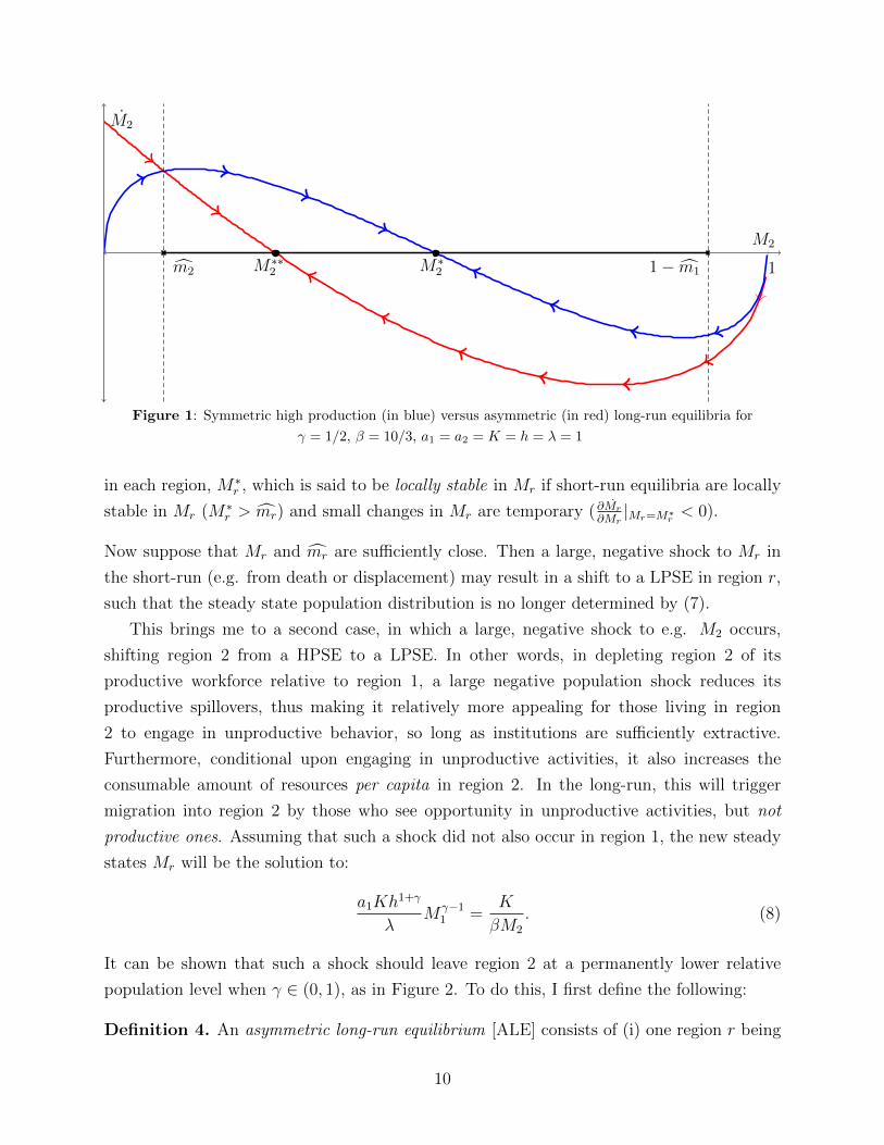
population level when γ ∈ (0, 1), as in Figure 2. To do this, I first define the following:

Definition 4. An asymmetric long-run equilibrium [ALE] consists of (i) one region r being

10

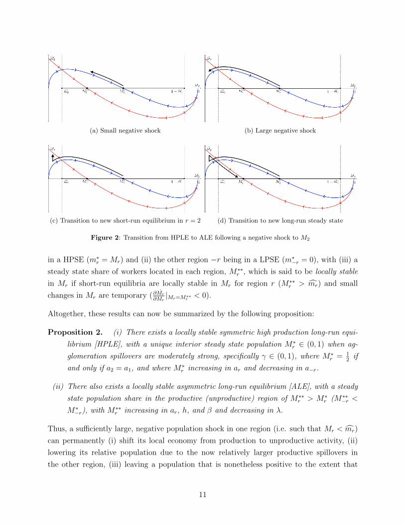
(a) Small negative shock (b) Large negative shock

(c) Transition to new short-run equilibrium in r = 2 (d) Transition to new long-run steady state

Figure 2: Transition from HPLE to ALE following a negative shock to M2

in a HPSE (m∗r = Mr) and (ii) the other region −r being in a LPSE (m∗−r = 0), with (iii) a

steady state share of workers located in each region, M∗∗r , which is said to be locally stable

in Mr if short-run equilibria are locally stable in Mr for region r (M∗∗r > mr) and small

changes in Mr are temporary (∂Mr

∂Mr|Mr=M∗∗

r< 0).

Altogether, these results can now be summarized by the following proposition:

Proposition 2. (i) There exists a locally stable symmetric high production long-run equi-

librium [HPLE], with a unique interior steady state population M∗r ∈ (0, 1) when ag-

glomeration spillovers are moderately strong, specifically γ ∈ (0, 1), where M∗r = 1

2if

and only if a2 = a1, and where M∗r increasing in ar and decreasing in a−r.

(ii) There also exists a locally stable asymmetric long-run equilibrium [ALE], with a steady

state population share in the productive (unproductive) region of M∗∗r > M∗

r (M∗∗−r <

M∗−r), with M∗∗

r increasing in ar, h, and β and decreasing in λ.

Thus, a sufficiently large, negative population shock in one region (i.e. such that Mr < mr)

can permanently (i) shift its local economy from production to unproductive activity, (ii)

lowering its relative population due to the now relatively larger productive spillovers in

the other region, (iii) leaving a population that is nonetheless positive to the extent that

11

its resources may still be utilized in relatively unproductive ways, with such payoffs being

determined by the quality of institutions (i.e. ∂mr∂β

< 0).12

In other words, given more extractive institutions, large-scale population loss tends to

induce a shift toward unproductive activities in the affected region by those remaining as well

as incoming migrants (e.g. property exploitation, corruption),13 rendering it less productive

and populated over the long-run. Stronger institutions, meanwhile, limit the extent to which

being production becomes relatively unappealing following large shocks, such that agents are

more likely to coordinate back to pre-shock patterns.

Lastly, let γ /∈ (0, 1). We know that when γ = 0, short-run shocks of any size should have

no bearing on short-run equilibria. Hence, sectors lacking agglomeration spillovers should

see their workers return to their pre-shock distribution, as determined by either (7) or (8).14

Remark 2. In the absence of agglomeration spillovers, γ = 0, population shocks have no

long-run effect on the spatial distribution of productive activity.

In other words, in sectors like agriculture which lack external economies of scale, shocks

have no permanent effects, regardless of institutions. Rather, the distribution of productive

activity is determined solely by the fundamentals. If fundamentals vary across space, then

activity will tend to locate more where they are stronger. If they are symmetric across

regions (i.e. a2 = a1), then so will be the distribution of e.g. farmers, both before and after

population shocks, assuming a HPLE to begin with.

What about when agglomeration spillovers are very strong, i.e. γ > 1?15 As it turns out,

when productive spillovers are sufficiently great, HPLE are always unstable:

Proposition 3. When agglomeration spillovers are sufficiently strong, specifically γ > 1,

then:

(i) There exists a symmetric high production long-run equilibrium [HPLE].

(ii) It is always unstable in Mr.

Hence, the existence of a locally stable HPLE is sufficient but not necessary for uneven

patterns of development to arise. Reminiscent of the new economic geography, when ag-

12Thus if a shock also negatively affects K over the long-run in that region, even fewer would reside there.13Alternatively, this could be thought of as corresponding to changes in local institutions or social norms.14As a corollary to Propositions 1 and 2, note that if institutions become too extractive, then unproductive

activities will become too appealing relative to productive ones, such that no HPLE or ALE can survive andboth regions will be in LPSE as part of a globally stable symmetric low production long-run equilibrium[LPLE]. To see this, note that the derivative on mr and those on both steady states M∗

r and M∗∗r are

opposing in β. For sufficiently low β, Mr ≥ mr can never occur, regardless of shocks.15I opt to ignore the trivial case where γ = 1, in which Mr is not well defined under equation (7).

12

glomeration spillovers are sufficiently strong, more interior equilibria tend toward instability,

in favor of unevenness over the long-run.16

The role of local development policy

Finally, note that in contrast with negative shocks, the model implies that the effects of

temporary local development policies and positive population shocks associated with them

(assuming an unproductive equilibrium to begin with) may actually be more likely to persist

in the long-run in places with strong institutions. This is because while it takes a negative

shock to mr larger than Mr − mr to move a region from a productive equilibrium to an

unproductive one, it takes a positive policy shock larger than mr to do the opposite. Hence,

when β is large, only a small-scale coordinated effort (e.g. by some “city corporation”) is

needed to move a region from an unproductive equilibrium to a productive one: an investment

need only attract a few to the region simultaneously before complementarities take over.

3 Empirical evidence

There exists a growing empirical literature exploring the short- and long-run impacts of

shocks on the location of economic activity, with war, expulsion, disease, and natural disaster

all serving as temporary shocks to relative city or region size (Davis and Weinstein, 2002;

Jedwab, Johnson, and Koyama, 2019; Kocornik-Mina et al, 2019; Testa, 2020). To the

extent that relative population levels and growth trends do not return to pre-shock levels,

as compared to places not exposed to the shock, it is taken as evidence in favor of multiple

spatial equilibria and the importance of increasing returns for determining differences in

development across space. At the same time, a sizable literature finds no such persistence

in the aftermath of even very large shocks, supporting a more deterministic view of spatial

development.

This paper proposes an interaction between increasing returns and a place’s underlying

formal17 institutions in determining its short- and long-run response to population shocks. In

the model, pre-shock equilibria are robust to even large shocks when institutions are strong.

To the extent that extractive institutions crowd out productive activities that generate in-

creasing returns, however, the model sees multiple equilibria emerge, with shocked places

experiencing a persistent relative decline in economic activity thereafter.

16For more on alternative equilibria when γ > 1, see Theory Discussion 2 in the Supplemental Material.17Although I focus on formal institutions, it is important to note that more informal institutions with

which they are correlated may also affect payoffs in the model and earthquake effects in this section.

13

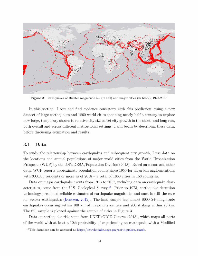
Figure 3: Earthquakes of Richter magnitude 5+ (in red) and major cities (in black), 1973-2017

In this section, I test and find evidence consistent with this prediction, using a new

dataset of large earthquakes and 1860 world cities spanning nearly half a century to explore

how large, temporary shocks to relative city size affect city growth in the short- and long-run,

both overall and across different institutional settings. I will begin by describing these data,

before discussing estimation and results.

3.1 Data

To study the relationship between earthquakes and subsequent city growth, I use data on

the locations and annual populations of major world cities from the World Urbanization

Prospects (WUP) by the UN’s DESA/Population Division (2018). Based on census and other

data, WUP reports approximate population counts since 1950 for all urban agglomerations

with 300,000 residents or more as of 2018 – a total of 1860 cities in 153 countries.

Data on major earthquake events from 1973 to 2017, including data on earthquake char-

acteristics, come from the U.S. Geological Survey.18 Prior to 1973, earthquake detection

technology precluded reliable estimates of earthquake magnitude, and such is still the case

for weaker earthquakes (Bentzen, 2019). The final sample has almost 8000 5+ magnitude

earthquakes occurring within 100 km of major city centers and 700 striking within 25 km.

The full sample is plotted against the sample of cities in Figure 3.

Data on earthquake risk come from UNEP/GRID-Geneva (2015), which maps all parts

of the world with at least a 10% probability of experiencing an earthquake with a Modified

18This database can be accessed at https://earthquake.usgs.gov/earthquakes/search.

14

Mercalli intensity (MMI) greater than V (i.e. moderate strength) within the next 50 years,

where MMI measures the effect of an earthquake at the surface.19 I consider a city as being

located in an earthquake risk area if such areas are within 50 km of its centroid. Under this

definition, 895 or about half of cities in the sample are assigned to earthquake risk areas.

To measure formal institutions, I use Polity IV’s (2019) POLITY index, which ranges

from -10 to 10. By their definition, a democracy is a country with a score of 6 or greater.

The advantage to using the POLITY index is that it consists of a long panel covering many

years and countries. Only three cities in the full sample are not covered by POLITY. One

concern, however, is that it provides a poor measure of institutions, in part because it reflects

contemporaneous political outcomes in addition to relatively “deep” institutional attributes

(Glaeser et al, 2004). To deal with this concern, I develop a time-invariant indicator of insti-

tutions, in which a city is considered to be in a “stable democracy” if it has consistently been

in a democracy under POLITY’s definition for the entire sample period. To the extent that

stable democracies tend to have stronger institutions than autocracies as well as relatively

unstable regimes (e.g. new or backsliding democracies), this should proxy for the deeper

institutional qualities with which the theory concerns itself.20

In secondary specifications, I also interact the treatment with a time-invariant indicator

of a city’s income level: its country’s income classification in 1990, midway through the

sample, as determined by the World Bank in their World Development Indicators (2019)

catalog.21 Countries with gross national income per capita below $2465 USD in 1990 are

considered low or lower-middle income, with the remainder of countries being upper-middle

or high income. I refer to cities in these two groups as low and high income, respectively.

3.2 Estimation

To estimate the immediate (i.e. following year) and longer-run impact of strong earthquakes

on city population growth, I adopt a distributed-lag approach that controls for a finite

number of lags on the explanatory variable (Dell, Jones, and Olken, 2012), using panel

19The four levels are >V, >VII, >VIII, and >IX. See Figure A.2 in the Supplemental Material for aheatmap of these areas, with darker orange corresponding to higher MMI scores with at least a 10% proba-bility of being exceeded, recreated using raster data available at https://preview.grid.unep.ch.

20A few countries in the sample were colonial territories (Angola, Djibouti, Guinea-Bissau, Mozambique,and Papua New Guinea) in the first few years of the sample and lack POLITY scores in those years. Similarly,since Berlin was divided until the end of the Cold War, it only enters the POLITY sample upon Germanreunification. I consider all of such cases as having experienced democracy and nondemocracy at varioustimes and code them as zeroes. I also derive alternative institutional measures using both POLITY and theWorld Governance Indicators (2020) rule of law and control of corruption indices, which I discuss below.

21See http://databank.worldbank.org/data/download/site-content/oghist.xls for these data.

15

Table 1: Summary Statistics, Subgroups

Subsample % City growth Earthquaket−1 Earthquake risk area Stable democracy

Full sample 3.418 0.008 0.481 0.291N= 83700 (3.265) (0.091) (0.500) (0.454)Earthquaket−1 = 1 2.867 – 0.969 0.283N= 700 (2.287) (0.175) (0.451)Earthquaket−1 = 0 3.423 – 0.477 0.291N= 83000 (3.271) (0.499) (0.454)Earthquake risk area = 1 3.403 0.017 – 0.287N= 40275 (2.965) (0.129) (0.453)Earthquake risk area = 0 3.432 0.001 – 0.295N= 43425 (3.520) (0.023) (0.456)Stable democracy 2.156 0.008 0.475 –N= 24345 (2.391) (0.090) (0.499)Not stable democracy 3.939 0.008 0.484 –N= 59220 (3.432) (0.092) (0.500)

Notes: Standard deviations in parentheses. For a complete list of summary statistics, see Table A.1 in the SupplementalMaterial. For map representations, see Figure A.3.

regressions of the following form:

∆Popit =L∑s=1

γsQuakei,t−s + θi +Yt + εit, (9)

where ∆Popit is a city’s rate of population growth between year t− 1 and year t; Quakei,t−s

is a dummy equal to one if an earthquake of 5+ magnitude on the Richter scale struck within

25 km of a city centroid in year t − s for s = 1, 2, ... up to some fixed number of lags L;

θi are city fixed effects; and Yt are year fixed effects, interacted separately with a national

income level dummy and a time-invariant earthquake risk dummy in main specifications.22

Regressions are robust to including various controls and interactions, as discussed below.

Errors εit are assumed to be spatially correlated beyond the city level (Conley, 2004; Hsiang,

2010). For main specifications, I use a distance cutoff of 300 km.23 Results are robust to

using alternative cutoffs as well as to clustering at the city or country level.

Spatial correlations in the frequency of earthquake activity may also give rise to hetero-

geneous effects.24 In particular, cities in areas regularly at risk of experiencing earthquakes

22Following comments received on previous drafts, all main specifications are now pooled and featureyear fixed effects with these interactions. Alternative specifications using institutions, region, and otherinteractions continue to be featured in the Supplemental Material, in Table A.5, as discussed below.

23This is based on the fact that contemporaneous treatment assignment may span such a radius, e.g.following tectonic structures spanning multiple cities (Tosi et al, 2008; Abadie et al, 2017).

24Of the 153 countries in the sample, only 64 (and only 13.7% of cities) experienced any major earthquakeat all, yet among those 64, 40 saw more than one strike within 25 km of a major city between 1973 and2017. Meanwhile, all years experienced such earthquakes, with a median of 15 per year, a mean of 15.6, anda standard deviation of 4.6 across years. This is consistent with Tosi et al (2008), who show that while thedistribution of seismicity across time is random at a global level, some areas are more prone to activity than

16

are likely to be different in relevant ways from those that do not. For instance, they may

be more prepared to deal with an earthquake, with better infrastructure or more funds allo-

cated toward post-earthquake recovery, which could attenuate effects (Neumayer, Plumper,

and Barthel, 2014). Since I am interested in the effects of exogenous and unexpected shocks

to city size, I also estimate regressions with a time-invariant earthquake risk dummy, which

I interact with Quakei,t−s for all s. This estimates separately the effects of an earthquake

on relative city growth in high-risk areas and in cities where it constitutes a relatively truer

shock.

3.3 Results

Table 2 examines the effect of earthquakes on city population growth, first without inter-

actions or lags. Columns (1) show that a one-off earthquake of 5+ magnitude is associated

with about a 0.1 percentage point decrease in a city’s rate of population growth the following

year. While this estimate is statistically significant, it lacks economic significance. Intro-

ducing lags in columns (2) sees this immediate effect estimated to be smaller still, reflecting

autocorrelation among lags.25 Then, in the years following an earthquake, dynamic effects

trend toward zero. Hence, when one utilizes the full sample of cities without differentiating

among them, the effect of a large, one-time earthquake shock on relative city growth appears

to be temporary and small at best.

The remainder of Table 2 accounts for a city’s time-invariant earthquake risk, estimating

the effects of earthquakes in high- and low-risk cities separately. Evaluating effects in cities

that historically experience few earthquakes, in which they are arguably more likely to serve

as an exogenous shock to city size, columns (3) reveal effects to be driven by these, with this

coefficient being much larger at about -1.1 (.37) pp. Moreover, when I introduce lags here, a

different trend emerges from before: the years following a one-off earthquake see persistent if

not increasing population growth decline, suggestive of a circular feedback process ongoing

in these cities as their relative sizes move to new equilibria.26 This trend persists if I add

additional lags, as shown in Table A.2 in the Supplemental Material.27 In contrast, summing

baseline and interaction coefficients reveals high-risk cities hardly respond at all, exhibiting

swift convergence back to pre-earthquake population levels with little cumulative effect,

others over the long-run (i.e. those near tectonic structures).25Hsiang and Jina (2014) discuss tradeoffs when choosing lags. Too few will bias estimates if omitted lags

are correlated with included ones, while adding lags will reduce bias but increase standard errors.26Another reason for relatively small instantaneous effects is that any interpolation used to derive popula-

tion counts between official reports would have averaged pre- and post-earthquake counts. Hence, measuredeffects may be largely capturing cases in which there was persistence (enough to be measurable years later).

27This finding mirrors Ager et al (2019), who find persistent changes to the spatial distribution of economicactivity in the American West following the 1906 San Francisco Earthquake.

17

Table 2: Effects of earthquakes on relative city growth

Annual city population growtht (%)No lags 3 lags

(1a) (1b) (2a) (2b)Earthquaket−1 -.124 -.124 -.099 -.099

(.070)∗ (.070)∗ (.071) (.071)

Earthquaket−2 – – -.072 -.072(.066) (.068)

Earthquaket−3 – – -.051 -.051(.070) (.071)

Earthquaket−4 – – -.029 -.029(.071) (.072)

Cumulative effect – – -.251 -.251(.139)∗ (.144)∗

Adj. R2 .134 .134 .146 .146With earthquake risk area dummy interaction

(3a) (3b) (4a) (4b)Earthquaket−1 -1.147 -1.147 -.521 -.521

(.371)∗∗∗ (.370)∗∗∗ (.166)∗∗∗ (.168)∗∗∗

Earthquaket−2 – – -.579 -.579(.145)∗∗∗ (.149)∗∗∗

Earthquaket−3 – – -.885 -.885(.267)∗∗∗ (.267)∗∗∗

Earthquaket−4 – – -1.075 -1.075(.365)∗∗∗ (.364)∗∗∗

Cumulative effect – – -3.060 -3.060(.608)∗∗∗ (.606)∗∗∗

Earthquaket−1×Earthquake risk 1.060 1.060 .434 .434(.377)∗∗∗ (.377)∗∗∗ (.181)∗∗ (.183)∗∗

Earthquaket−2×Earthquake risk – – .519 .519(.160)∗∗∗ (.164)∗∗∗

Earthquaket−3×Earthquake risk – – .864 .864(.276)∗∗∗ (.277)∗∗∗

Earthquaket−4×Earthquake risk – – 1.084 1.084(.372)∗∗∗ (.371)∗∗∗

Cum. interaction×Earthquake risk – – 2.900 2.900(.624)∗∗∗ (.624)∗∗∗

Adj. R2 .134 .134 .146 .146Observations 83700 83700 78120 78120Conley S.E. cutoff 100 km 300 km 100 km 300 km

Notes: Standard errors are robust to spatial correlation up to the distance specified, according to a uniform spatial weightingkernel, with ***, **, and * denoting significance at the 1%, 5%, and 10% levels, respectively. All specifications include city,year×income level, and year×earthquake risk fixed effects. An earthquake is considered to have hit a city if it struck within 25km of that city’s centroid in the previous year. “Earthquake risk” is a dummy that equals 1 if there is at least a 10% probabilityof a city experiencing an MMI event greater than V in the next 50 years at any point within 50 km of its centroid. Baselineeffects in the second set of results represent effects in low-risk cities. Interaction estimates represent the difference betweeneffects in low- and high-risk cities.

18

Table 3: Short-run effects of earthquakes by institutions

(1) (2) (3) (4)Earthquaket−1 -1.147 -1.484 -1.356 -.870

(.370)∗∗∗ (.468)∗∗∗ (.432)∗∗∗ (.285)∗∗∗

Earthquaket−1×Stable democracy – 1.096 1.160 1.403(.511)∗∗ (.492)∗∗ (.548)∗∗∗

Earthquaket−1×Earthquake risk 1.060 1.396 1.301 .807(.377)∗∗∗ (.475)∗∗∗ (.439)∗∗∗ (.297)∗∗∗

Earthquaket−1×Stable democracy×Risk – -1.093 -1.010 -1.288(.535)∗∗ (.501)∗∗ (.571)∗∗

Earthquaket−1×Income level – – -.275 -1.326(.169) (.572)∗∗

Earthquaket−1×Income×Risk – – – 1.116(.598)∗

Adj. R2 .134 .134 .134 .134Observations 83700 83565 83565 83565Income level interaction? No No Yes YesIncome×risk interaction? No No No Yes

Notes: Standard errors are robust to spatial correlation up to a distance of 300 km, according to a uniform spatial weightingkernel, with ***, **, and * denoting significance at the 1%, 5%, and 10% levels, respectively. All specifications include city,year×income level, and year×earthquake risk fixed effects. An earthquake is considered to have hit a city if it struck within 25km of that city’s centroid in the previous year. “Earthquake risk” is a dummy that equals 1 if there is at least a 10% probabilityof a city experiencing an MMI event greater than V in the next 50 years at any point within 50 km of its centroid. “Stabledemocracy” is a dummy that equals 1 if the country in which a city resides was consistently a democracy during the sampleperiod. “Income level” is a dummy that equals 1 if the country in which a city resides was classified as high or upper-middleincome in 1990. Baseline effects represent effects with dummies set to 0.

suggesting greater preparedness in such places re-coordinating activity post-quake.

The second exercise I perform with the data seeks to test the model’s key prediction:

that the relative amount of economic activity will be less robust to shocks in places with

weaker or more extractive institutions. If the logic of the model is correct, one would expect

the effects of earthquakes on relative city size to be driven disproportionately by the cities

located outside of stable democracies, in autocracies as well as relatively unstable regimes.

The estimates in Tables 3 and 4 suggest this to be the case. Looking first at short-run

effects, columns (2-4) in Table 3 show negative and statistically significant effects for such

cities after accounting for earthquake risk. In particular, estimates show an initial decrease

in annual city population growth of about 0.9-1.5 pp associated with a nearby earthquake

for low-risk cities outside of stable democracies, with positive and statistically significant

interaction coefficients for cities in stable democracies, suggesting overall effects are being

driven by the former.

Similar patterns are observed upon the inclusion of lags, as shown in Table 4. After

accounting for earthquake risk, long-run effects mirror those in Table 2 for cities not located in

stable democracies, with negative and increasing effects over time for a four-year cumulative

effect of −2.5 to −3.7 pp, mirroring the findings in Barone and Mocetti (2014) on a global

scale. In contrast, interaction coefficients again cancel out after a few years for cities in

19

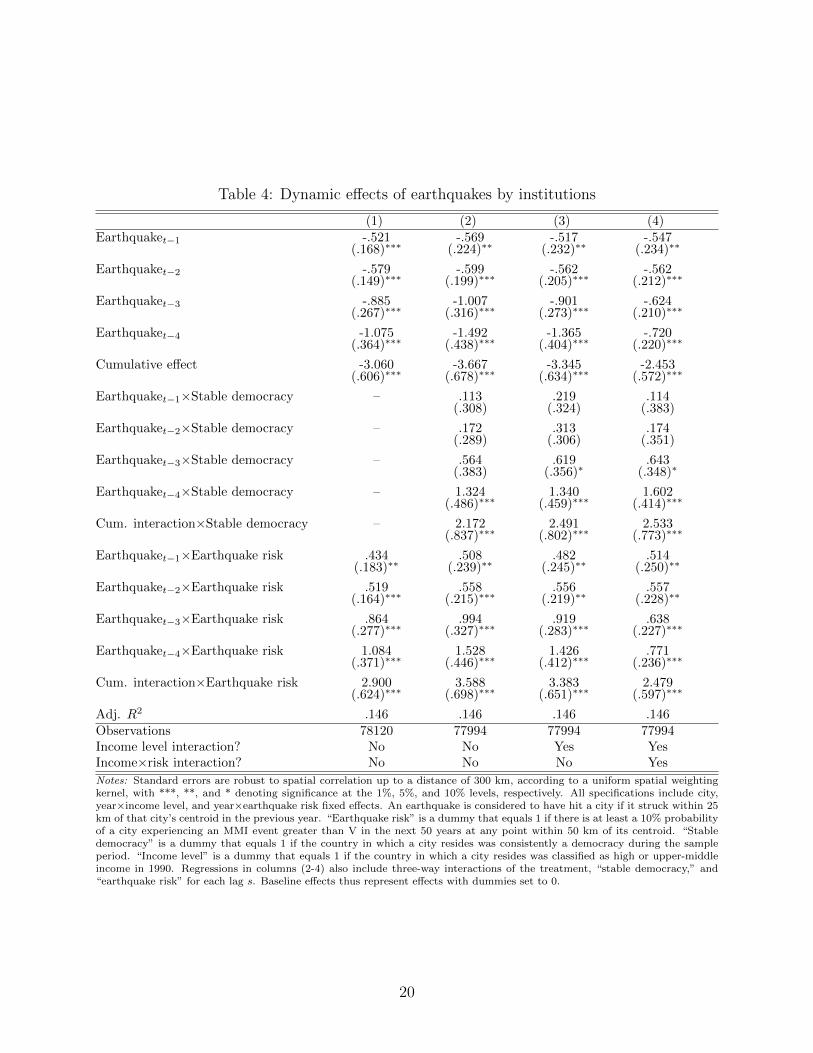
Table 4: Dynamic effects of earthquakes by institutions

(1) (2) (3) (4)Earthquaket−1 -.521 -.569 -.517 -.547

(.168)∗∗∗ (.224)∗∗ (.232)∗∗ (.234)∗∗

Earthquaket−2 -.579 -.599 -.562 -.562(.149)∗∗∗ (.199)∗∗∗ (.205)∗∗∗ (.212)∗∗∗

Earthquaket−3 -.885 -1.007 -.901 -.624(.267)∗∗∗ (.316)∗∗∗ (.273)∗∗∗ (.210)∗∗∗

Earthquaket−4 -1.075 -1.492 -1.365 -.720(.364)∗∗∗ (.438)∗∗∗ (.404)∗∗∗ (.220)∗∗∗

Cumulative effect -3.060 -3.667 -3.345 -2.453(.606)∗∗∗ (.678)∗∗∗ (.634)∗∗∗ (.572)∗∗∗

Earthquaket−1×Stable democracy – .113 .219 .114(.308) (.324) (.383)

Earthquaket−2×Stable democracy – .172 .313 .174(.289) (.306) (.351)

Earthquaket−3×Stable democracy – .564 .619 .643(.383) (.356)∗ (.348)∗

Earthquaket−4×Stable democracy – 1.324 1.340 1.602(.486)∗∗∗ (.459)∗∗∗ (.414)∗∗∗

Cum. interaction×Stable democracy – 2.172 2.491 2.533(.837)∗∗∗ (.802)∗∗∗ (.773)∗∗∗

Earthquaket−1×Earthquake risk .434 .508 .482 .514(.183)∗∗ (.239)∗∗ (.245)∗∗ (.250)∗∗

Earthquaket−2×Earthquake risk .519 .558 .556 .557(.164)∗∗∗ (.215)∗∗∗ (.219)∗∗ (.228)∗∗

Earthquaket−3×Earthquake risk .864 .994 .919 .638(.277)∗∗∗ (.327)∗∗∗ (.283)∗∗∗ (.227)∗∗∗

Earthquaket−4×Earthquake risk 1.084 1.528 1.426 .771(.371)∗∗∗ (.446)∗∗∗ (.412)∗∗∗ (.236)∗∗∗

Cum. interaction×Earthquake risk 2.900 3.588 3.383 2.479(.624)∗∗∗ (.698)∗∗∗ (.651)∗∗∗ (.597)∗∗∗

Adj. R2 .146 .146 .146 .146Observations 78120 77994 77994 77994Income level interaction? No No Yes YesIncome×risk interaction? No No No Yes

Notes: Standard errors are robust to spatial correlation up to a distance of 300 km, according to a uniform spatial weightingkernel, with ***, **, and * denoting significance at the 1%, 5%, and 10% levels, respectively. All specifications include city,year×income level, and year×earthquake risk fixed effects. An earthquake is considered to have hit a city if it struck within 25km of that city’s centroid in the previous year. “Earthquake risk” is a dummy that equals 1 if there is at least a 10% probabilityof a city experiencing an MMI event greater than V in the next 50 years at any point within 50 km of its centroid. “Stabledemocracy” is a dummy that equals 1 if the country in which a city resides was consistently a democracy during the sampleperiod. “Income level” is a dummy that equals 1 if the country in which a city resides was classified as high or upper-middleincome in 1990. Regressions in columns (2-4) also include three-way interactions of the treatment, “stable democracy,” and“earthquake risk” for each lag s. Baseline effects thus represent effects with dummies set to 0.

20

stable democracies. Both annual and cumulative baseline effects for cities in and outside of

stable democracies can be seen visually in Figure A.4 in the Supplemental Material.

One concern is that stable democracy is positively associated with wealth. Since reactions

to earthquakes likely vary in rich versus poor countries, it is possible that controlling for

national income level could account for differences associated with formal institutions above.

Columns (3) and (4) in Tables 3 and 4 include this interaction alongside the institutions

one. Significant interaction effects from institutions persist in all cases. Interestingly, cities

in higher income countries tend to exhibit more negative effects, as shown in Table 3. This

potentially reflects the economic ease of migration in response to negative shocks in such

places, relative to cities in lower income countries.

Results are also robust to including other city-year controls. Potentially important inter-

actions include earthquake depth and Richter magnitude as well as a city’s distance from the

nearest other major city. For instance, Richter magnitude and quake depth tend to increase

and decrease the surface effects of earthquakes, respectively, while Bosker et al (2017) show

that spatial interdependencies between cities can impact the effects of shocks. Effects with

these interactions included can be found in Table A.4 in the Supplemental Material.

Another important assumption is the choice of year fixed effects. The preferred specifi-

cation lets time effects vary by both national income level and earthquake risk, on the basis

that such factors are likely to impact a city’s population growth over time. In the Supple-

mental Material, I explore several alternative fixed effects assumptions, including different

combinations of (i) year×income level, (ii) year×earthquake risk, (iii)year×institutions, and

(iv) year×region dummies.28 Point estimates are substantively similar across specifications

while precision varies, with those that control for heterogeneity across institutions and/or

income groups yielding more precise estimates. In contrast, estimates lose precision when I

do not interact fixed effects or interact them only with region dummies, with little earth-

quake variation existing within regions, particularly outside of Asia and the Americas, and

much important variation in income, institutions, and other relevant unobservables existing

within each region. These estimates can be found in Table A.5.

Alternative institutions measures

Thus far, the paper has used Polity IV’s (2019) POLITY index to measure institutions.

Instead of using a city’s country’s POLITY score, however, I develop a time-invariant indi-

cator which considers a city’s entire history over the 1973-2017 period, in order to capture

relatively “deep” institutional attributes rather than contemporaneous political outcomes.

The POLITY index is thus ideal on the basis that it spans this entire period.

28Regions used are Africa, Asia, Oceania, Europe, and the Americas.

21

Results are robust, however, to using alternative measures of institutions. First, I use

the POLITY index to construct two alternative measures of institutions. The first instead

uses a cutoff POLITY score of zero to define “stable democracy,” while the second allows

institutions to vary over time if the state in which the city resided changed in the POLITY

index (e.g. Prague resided in Czechoslovakia, a communist autocracy, through 1992, after

which it resided in the Czech Republic, a parliamentary republic).29 These results can be

found in columns (1a-2b) of Table A.6 in the Supplemental Material.

The second set of alternative measures uses indices from the World Governance Indicators

(2020) report, which only covers 1996 to the present. I examine two measures of institutions

relevant to the model: (i) rule of law and (ii) control of corruption.30 For each of these, I

construct a measure analogous to the paper’s main measure, in which a city is given a value

of 1 if it is in a country that has consistently had a positive standardized score in that index

through 2017. Encouragingly, the interaction effects here bear the same signs as those of the

POLITY measure, though estimates tend to be smaller, with effects becoming statistically

significant after 3 years. These results can be found in columns (3a-4b) of Table A.6.

Event-study specification and pre-trends

Although a distributed-lag model is commonly used to study the effects of phenomena with

multiple or repeated events as in this paper (Hsiang and Jina, 2014; Dell, Jones, and Olken,

2012; Cerra and Saxena, 2008), an alternative approach would be to adopt an event-study

difference-in-differences design, in which event time is defined around earthquake years. This

would enable estimation of pre-trends leading up earthquake shocks as further evidence of

their exogeneity. Yet it may also produce biased estimates if cities have multiple earth-

quakes in close proximity, each with its own effect and with pre- and post-treatment effects

overlapping.

I mitigate this latter concern by estimating the dynamic treatment effects of the first

earthquake in each treated city’s observation window spanning 1973 to 2017. To further

reduce bias from earthquakes immediately preceding the observation window, which could

generate the appearance of pre-trends, I limit the effect window to three relatively balanced

29Relatedly, when I split the sample of cities not in stable democracies into those in stable nondemocracies(POLITY< 6 for all years) and those in neither stable democracies nor stable nondemocracies (i.e. unstablepolities), the same patterns persist in both samples, as shown in Tables A.7. To the extent that effects reflectthe importance of formal institutions, this affirms the presumption that transitioning and young democraciesdo not necessarily have strong underlying deep institutional qualities. However, due to limited observationsas subgroups increase, I do not emphasize these estimates.

30While rule of law pertains to important dimensions such as the protection of property rights, corruptionis a key “unproductive” activity that comes up repeatedly not only in the earthquake case studies below butin prior research on earthquake effects (Ambraseys and Bilham, 2011; Barone and Mocetti, 2014).

22

pre-periods (including the omitted period), before which < 80% of treated cities have ob-

servable pre-periods. Similarly, as post-earthquake periods are increasingly likely to estimate

the effects of subsequent earthquakes, I limit post-periods to four, as in the distributed-lag

model. Lastly, such factors are less likely to be problematic upon considering cities outside

of earthquake risk areas. The event-study framework thus estimates the following:

∆Popit =−1∑s=−2

γsFirstQuakei,t−s +4∑s=1

γsFirstQuakei,t−s + θi +Yt + εit,

where s = 0, the year in which the earthquake occurred, is the omitted period (i.e. γ0 = 0

imposed), to which effects for all fully post-treatment years γs>0 as well as pre-trends γs<0 are

relative. Remaining observations outside the effect window are binned, serving as additional

controls in the estimation of dynamic effects alongside never-treated observations. As in the

distributed-lag model, I let time effects vary by national income level and earthquake risk.

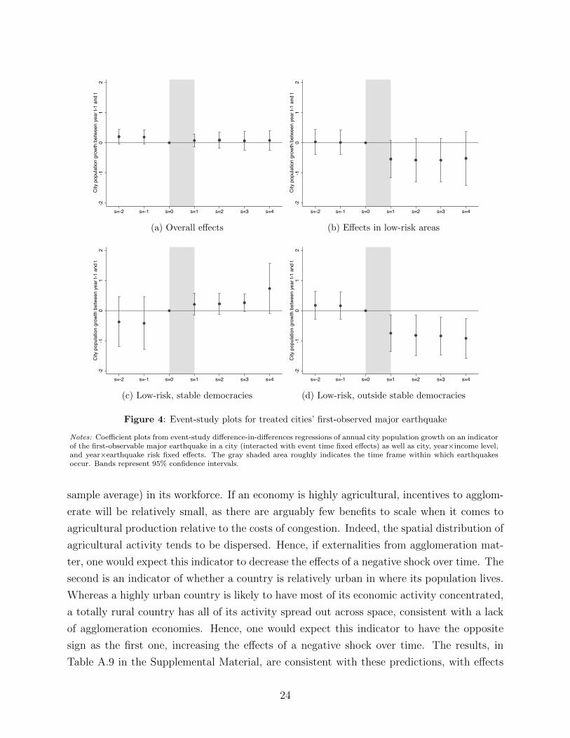
I plot event-study estimates from three variants of this model. The first analyzes overall

effects (Figure 4, top left); a second accounts for earthquake risk (Figure 4, top right);

and a third lets effects vary by institutions (Figure 4, bottom row). Estimated pre-trends

lack statistical significance in all cases, though one might argue subtle trends exist between

s = −1 and s = 0. This likely reflects the fact that population effects may occasionally occur

in the omitted year, i.e. if the earthquake happened quite early in the year. Post-treatment

effects are similar to distributed-lag estimates using the full set of quakes, with only cities

outside stable democracies exhibiting persistent negative effects.

Agglomeration economies

A secondary prediction of the model is that agglomeration spillovers remain a necessary con-

dition for a population shock to have persistent effects, regardless of institutions (see Remark

2). This has implications for local economies dominated by sectors such as agriculture that

are not generally associated with external economies of scale – that is, one would not expect

effects to persist in such economies. Although this section examines cities, on the basis that

their existence is generated associated with agglomeration economies (Glaeser and Gottlieb,

2009; Bleakley and Lin, 2012), the extent to which such spillovers matter for effects has thus

far been taken for granted in the empirical analysis. Unfortunately, there are no measures

of agglomeration economies across cities with which to match the dataset. Data do exist,

however, which can roughly capture the extent to which such incentives to agglomerate are

present in the country in which each city is located. I derive two such measures.

The first is an indicator of whether a country is relatively agricultural (i.e. above the

23

-2-1

01

2C

ity p

opul

atio

n gr

owth

bet

wee

n ye

ar t-

1 an

d t

s=-2 s=-1 s=0 s=1 s=2 s=3 s=4

(a) Overall effects

-2-1

01

2C

ity p

opul

atio

n gr

owth

bet

wee

n ye

ar t-

1 an

d t

s=-2 s=-1 s=0 s=1 s=2 s=3 s=4

(b) Effects in low-risk areas

-2-1

01

2C

ity p

opul

atio

n gr

owth

bet

wee

n ye

ar t-

1 an

d t

s=-2 s=-1 s=0 s=1 s=2 s=3 s=4

(c) Low-risk, stable democracies

-2-1

01

2C

ity p

opul

atio

n gr

owth

bet

wee

n ye

ar t-

1 an

d t

s=-2 s=-1 s=0 s=1 s=2 s=3 s=4

(d) Low-risk, outside stable democracies

Figure 4: Event-study plots for treated cities’ first-observed major earthquake

Notes: Coefficient plots from event-study difference-in-differences regressions of annual city population growth on an indicatorof the first-observable major earthquake in a city (interacted with event time fixed effects) as well as city, year×income level,and year×earthquake risk fixed effects. The gray shaded area roughly indicates the time frame within which earthquakesoccur. Bands represent 95% confidence intervals.

sample average) in its workforce. If an economy is highly agricultural, incentives to agglom-

erate will be relatively small, as there are arguably few benefits to scale when it comes to

agricultural production relative to the costs of congestion. Indeed, the spatial distribution of

agricultural activity tends to be dispersed. Hence, if externalities from agglomeration mat-

ter, one would expect this indicator to decrease the effects of a negative shock over time. The

second is an indicator of whether a country is relatively urban in where its population lives.

Whereas a highly urban country is likely to have most of its economic activity concentrated,

a totally rural country has all of its activity spread out across space, consistent with a lack

of agglomeration economies. Hence, one would expect this indicator to have the opposite

sign as the first one, increasing the effects of a negative shock over time. The results, in

Table A.9 in the Supplemental Material, are consistent with these predictions, with effects

24

disappearing after three periods for cities in agricultural and rural countries and otherwise

continuing to grow. This suggests the persistence of effects here are indeed rooted in the

presence of externalities from the agglomeration of activity, as opposed to simply following

a random walk a la Gabaix (1999).

3.4 Discussion

Though interaction effects from measures of institutions corroborate the theory presented

above, it remains to be seen whether the effects observed here are indeed rooted in shifts to-

ward unproductive behavior in the aftermath of earthquakes – such as corruption in the local

public sector or property crime in the absence of strong enforcement, which in turn prolong

the effects of the initial shock – or other unobservable factors associated with institutions.

Some qualitative support for this mechanism can be found by examining notable major

earthquakes in recent history. In this section, I analyze four such events: (i) the January 2010

earthquake near Port-au-Prince, Haiti; (ii) the May 2008 earthquake in Sichuan, China, out-

side of Chengdu; (iii) the February 2010 earthquake north of Concepcion, Chile; and (iv) the

March 2011 earthquake off the coast of Sendai, Japan. I choose to focus on these earthquakes

as each generated significant (negative or positive) analysis among the press, highlighting

the different local political and economic responses that followed them. Underlying these

differences, I will argue, is significant variation in the institutional qualities of the countries

in which each took place (e.g. in the rule of law, control of corruption, etc.), while the

importance of such differences is evident in the economic dynamics that followed.

2010 Haiti earthquake

On January 12, 2010, a magnitude 7.0 earthquake struck about 25 km outside of Port-au-

Prince, Haiti. Though the island has a history of destructive earthquakes, this earthquake

was particularly shallow and, given its close proximity to a major urban area of nearly 3

million people, severe damage was unavoidable (Hou and Shi, 2011).

Aftermath. At the time of the earthquake, Haiti was one of the poorest and least developed

countries in the world, leaving it vulnerable to higher death tolls and destruction. In the end,

upwards of 316,000 died in the quake, alongside 300,000 injured and 1.5 million displaced,

with somewhere between 1.5 and 4.5 million affected in total. Estimates of direct economic

loss range from 7.8-13.9 billion USD (Hou and Shi, 2011; Assessing Progress in Haiti Act,

2014). Given this, the Haitian government relied heavily on international support for relief

and reconstruction, with about $13.5 billion donated or pledged from foreign governments

25

and private charities in total (Assessing Progress in Haiti Act, 2014).

Beyond poverty, however, the depth of the crisis can also be attributed to a “lack of

social structures [and] weak political system that lacks both efficiency and legitimacy” (Hou

and Shi, 2011, 28), with weak institutions giving rise to corrupt and unproductive uses of

resources and recovery funds. Government teams were mobilized slowly and in low numbers,

with bodies and debris remaining in the streets for days after the quake. Police responses

were also limited; of the 6000 police directed to Port-au-Prince after the quake, just over

half actually arrived. Nor were police efficacious in bringing calm; days after the earthquake,

police opened fire on rioters and looters who had emerged in the quake’s aftermath (Hou and

Shi, 2011). And in the years since, large amounts of aid have gone unallocated to affected

communities. Beyond corrupt uses of funds by local officials, an NPR (2015) report docu-

ments how a lack of trust in the local use of funds led to a reliance on outside contractors,

slowing dispersal and inflating costs.

Effects. Haiti continues to experience direct and indirect effects of the earthquake today.

Thousands remained displaced, living in “makeshift camps, with no power or running water,”

according to one Al Jazeera report (2020). Haitian refugees also continue to flow into nearby

countries, such as Brazil as well as Ecuador and Peru (Miura, 2014; Fagen, 2013). And

population growth in Port-au-Prince seems to have slowed indefinitely. In the WUP data,

Port-au-Prince enjoyed population growth of just over 5% annually in the decade leading up

to the earthquake. After 2010, which saw the city lose 19% of its population, its growth rate

has remained around 2.6% – a nearly 50% decline from pre-quake trends.

2008 Sichuan earthquake

In May of 2008, an earthquake of Richter magnitude 8.0 hit the Wenchuan area of Sichuan,

China (Zifa, 2008). Its epicenter was about 80 km from Sichuan’s largest city and provin-

cial capital of Chengdu, which had a population of about 14 million in 2010, with the next

largest cities in the province located further away. Importantly, an earthquake of this size

was unexpected and buildings in the area generally had relatively low seismic resistance.

Aftermath. The impact of the quake was immediately felt. Though estimates suggest 68-

88,000 died in the earthquake, hundreds of millions were affected in the form of displacements,

property damage, etc. (Yang et al, 2014). In terms of economic losses, initial estimates of

direct property losses ranged from 98-500 billion RMB (the equivalent of 14-70 billion 2020

USD), making it one of the more destructive earthquakes in modern history (Zifa, 2008).

Other consequences were less direct. Several scandals unfolded in the wake of the quake,

26

most notably in the construction and public sectors. Although 3800 new schools and housing

for 1.9 million households were constructed in the aftermath, an NPR (2013) investigation

found that many of the new builds did not meet the new earthquake standards required by

law, with “cracks [appearing] before any major tremors.” Other corners were cut as well,

in the form of unpaid worker salaries and projects finished months ahead of schedule. Co-

inciding with this was the illegal use of at least $228 million in reconstruction funds, with

one low-level official being charged with $1.7 million in bribery. A report by the South

China Morning Post (2018) documents how reconstruction budgets were inflated, costs over-

reported, and billions of yuan embezzled via repeated filings for relief aid by local bureaus.

Effects. The effects of the Sichuan earthquake were highly regional, with changes in the dis-

tribution of economic activity occurring within the province of Sichuan thereafter. Although

the earthquake’s epicenter was about 80 km northwest of Chengdu, affected populations

resided disproportionately around Chengdu and in areas to its east (Jia et al, 2018). The

same areas saw significant population decline between 2005 and 2012, as high as 5% in some

counties, with less affected counties continuing to see significant population growth over the

same period (Yang, Han, and Song, 2014). In Chengdu itself, population growth in the WUP

data sees slowdown beginning in 2010, with more in the following years. Whereas population

growth in Chengdu had been just over 5% prior to the earthquake, by 2012 it was about

1.8%, around which it has remained since, a trend I do not observe in other Sichuan cities.

2010 Chile earthquake

Not all major earthquakes are associated with criminal or corrupt activity in their after-

maths. One such counterexample is the 2010 Chile earthquake, which was felt most strongly

in the city of Concepcion, about 100 km to the south of the quake’s epicenter. Occurring

just one month after the Port-au-Prince earthquake, Chile’s quake was 8.8 in magnitude and

felt throughout the country (Hombrados, 2020).

Aftermath. Despite destructive beginnings, with economic damages of about 15-30 billion

USD, Chile’s government was praised in the press for its disaster response, and only 547

fatalities were reported (Hombrados, 2020). News coverage in TIME (2010) and Brookings

(2010) compared the conditions that followed favorably to those in Port-au-Prince, noting

the swift allocation of government resources and an absence of corruption in the country’s

construction and public sectors, as evidenced by strong enforcement of building codes. An-

other article by Warren (2010) likewise lauded Chile’s aid response but criticized its ability

to protect property rights and restore public order in face of post-quake vandalism and loot-

27

ing. However, this narrative is empirically questioned by Hombrados (2020), who finds that

the incidence of property crime actually decreased in areas exposed to more intense tremors,

driven by strong community-based crime-prevention mechanisms.

Effects. Although Chile frequently experiences earthquakes and is infrastructurally prepared

for such disasters, the effects of this particular earthquake – which at a magnitude of 8.8 was

about 500 times more powerful than the one in Port-au-Prince – are not a priori clear. As it

turns out, population growth in Concepcion as well as all other major Chilean agglomerations

is remarkably stable in the WUP data in the years following the earthquake, relative to pre-

quake trends.

2011 Sendai earthquake

The 9.0 magnitude earthquake that struck off the coast of Sendai, Japan in March 2011

generated similar commentary in the press. That earthquake, which also produced extensive

tsunamis, was declared the “toughest and the most difficult crisis for Japan” since WWII by

the prime minister and, like the Port-au-Prince quake, affected the entire main island (Clark

and Heath, 2014).

Aftermath. Though much of Japan is earthquake prone, the earthquake’s magnitude and

subsequent tsunamis made it highly destructive, killing over 15,000 across 20 prefectures

and damaging over a million buildings,31 with economic damages of up to $235 billion (Kim,

2011). Despite such initial destruction, however, press reports mirrored the positive response

that had followed the Chile earthquake the previous year. One Brookings (2011) report ar-

gued that Japan’s strict enforcement of building codes, its strong control of corruption, and

low property crime in the aftermath of the disaster favored a quick local recovery, while

criticizing the government’s response to the nuclear accidents that followed the disaster. An

NPR (2011) report similarly pointed to strong enforcement of building codes by officials and

a corresponding lack of corruption and bribery in the construction sector as being key to

Japan’s recovery relative to Haiti’s and Sichuan’s, with Japan and Chile both emerging with

far fewer deaths despite suffering far more severe quakes.

Effects. As with Chile’s earthquake a year prior, the effects of the Sendai disaster appear

to have had little impact on the spatial distribution of economic activity within Japan or

population growth in affected areas. In Sendai, the largest major city in close proximity to

31Statistics are made available by the National Police Agency of Japan athttps://www.npa.go.jp/news/other/earthquake2011/pdf/higaijokyo e.pdf.

28

the quake, the WUP data actually sees population growth go from about -1.1% annually in

the years leading up to the quake, to about 0.8% annually afterward.

4 Conclusion

Why do some shocks to local development permanently impact the spatial distribution of

economic activity, while others do not? This paper considers the role of formal institutions in

explaining these differential effects. In the model, extractive institutions decrease the return

on productive relative to unproductive activities. In the presence of increasing returns to

productive activity within regions, a sufficiently large, negative shock to one region’s labor

force can serve as a tipping point, inducing its workers to substitute into unproductive

activities. Thereafter, new migrants will also prefer to engage in unproductive activities,

resulting in regional asymmetries in population and production levels over the long-run. This

suggests that extractive institutions may magnify the importance of increasing returns for

long-run local development, while long-run equilibria may be more robust to large negative

shocks where there are strong institutions to help coordinate the reemergence of production.

An empirical examination into the effects of large earthquakes on population growth in major

world cities finds suggestive evidence for these predictions.

I conclude with a few remarks. First, it is important to note that the choice between

productive and unproductive activity is, in reality, not binary. Rather, the prevalence of the

latter will depend on its relative return as determined by the institutional environment (i.e.

β). As institutions improve, it seems likely that even unproductive regions would become

more developed. Nor is this stylized model sufficient to explain all differences in development

observed within countries. A richer model is needed to capture the nuanced interactions

between institutions, agglomeration spillovers, natural geography, infrastructure, etc. That

being said, this model illustrates in simple terms how formal institutions can influence the

importance of increasing returns in the face of large shocks. In particular, it suggests that

spatial equilibria may be more subject to influence by negative shocks in places and times

in which institutions are weak, becoming more robust as they improve.

References

[1] Abadie, A. S. Athey, G. W. Imbens, and J. Wooldridge (2017). When should you adjust yourstandard errors for clustering? Working Paper.

[2] Acemoglu, D. (1995). Reward structures and the allocation of talent. European EconomicReview. 39, 17-33.

29

[3] Acemoglu, D. and M. Dell (2010). Productivity differences between and within countries.American Economic Journal: Macroeconomics. 2, 169-88.

[4] Acemoglu, D., G. de Feo, and G. D. de Luca (2019). Weak states: Causes and consequencesof the Sicilian Mafia. Review of Economic Studies. 97, 537-81.

[5] Acemoglu, D., Johnson, S. and Robinson, J.A. (2001). The colonial origins of comparativedevelopment: An empirical investigation. American Economic Review. 91, 1369-401.

[6] Acemoglu, D., T. A. Hassan, and J. A. Robinson (2011). Social structure and development:A legacy of the Holocaust in Russia. Quarterly Journal of Economics. 126, 895-946.

[7] Acemoglu, D., F. A. Gallego, and J. A. Robinson (2014). Institutions, human capital, anddevelopment. Annual Review of Economics. 6, 875-912.

[8] Ager, P., K. Eriksson, C. W. Hansen, and L. Lonstrup (2019). How the 1906 San FranciscoEarthquake shaped economic activity in the American West. Working Paper.

[9] Ahlerup, P. (2013). Are natural disasters good for economic growth? Working Paper.

[10] Allen, T. and D. Donaldson (2018). The geography of path dependence. Working Paper.

[11] Ambraseys, N. and R. Bilham (2011). Corruption kills. Nature. 469, 153-5.

[12] Anbarci, N., M. Escaleras, and C. A. Register (2005). Earthquake fatalities: The interactionof nature and political economy. Journal of Public Economics. 89, 1907-33.

[13] Assessing Progress in Haiti Act of 2014 (2014). U.S. Congress. S. 1104 (113th).https://www.govtrack.us/congress/bills/113/s1104/text.

[14] Barone, G., and S. Mocetti (2014). Natural disasters, growth and institutions: A tale of twoearthquakes. Journal of Urban Economics. 84, 52-66.

[15] Belloc, M., F. Drago, and R. Galbiati (2016). Earthquakes, religion, and transition to self-government in Italian cities. Quarterly Journal of Economics. 131, 1875-926.

[16] Bentzen, J. S. (2019). Acts of God? Religiosity and natural disasters across subnational worlddistricts. Economic Journal. 129, 2295-2321.

[17] Bleakley, H. and J. Lin (2012). Portage and path dependence. Quarterly Journal of Economics.127, 587-644.

[18] Bosker, M., S. Brakman, H. Garretsen, and M. Schramm (2007). Looking for multiple equi-libria when geography matters: German city growth and the WWII shock. Journal of UrbanEconomics. 61, 152-67.

[19] Boustan, L. P., M. E. Kahn, P. W. Rhode, and M. L. Yanguas (2017). The effect of natural dis-asters on economic activity in U.S. counties: A century of data. Journal of Urban Economics.Forthcoming.

[20] Brakman, S., H. Garretsen, and M. Schramm (2004). The strategic bombing of German citiesduring WWII and its impact on city growth. Journal of Economic Geography. 4, 201-18.

30

[21] Cavallo, E., S. Galiani, I. Noy, and J. Pantano (2013). Catastrophic natural disasters andeconomic growth. Review of Economics and Statistics. 95, 1549-61.

[22] Cerra, V. and S. C. Saxena (2008). Growth dynamics: The myth of economic recovery. Amer-ican Economic Review. 98, 439-57.

[23] Chaney, E. and R. Hornbeck (2016). Economic dynamics in the Malthusian era: Evidencefrom the 1609 Spanish expulsion of the Moriscos. Economic Journal. 126, 1404-40.

[24] Clark, T. and A. Heath (2014). Hard Times: The Divisive Toll of the Economic Slump. NewHaven: Yale University Press.

[25] Conley, T. (1999). GMM estimation with cross sectional dependence. Journal of Econometrics.92:1-45.

[26] Davis, D. R. and D. E. Weinstein (2002). Bones, bombs, and break points: The geography ofeconomic activity. American Economic Review. 92, 1269-89.

[27] – (2008). A search for multiple equilibria in urban industrial structure. Journal of RegionalScience. 48, 29-65.

[28] Dell, M. (2010). The persistent effects of Peru’s mining mita. Econometrica. 78, 1863-1903.

[29] Dell, M., B. F. Jones, and B. A. Olken (2012). Temperature shocks and economic growth:Evidence form the last half century. American Economic Journal: Macroeconomics. 4, 66-95.

[30] Dell, M. and B. A. Olken (2019). The development effects of the extractive colonial economy:The Dutch Cultivation System in Java. Review of Economic Studies. 87, 164-203.

[31] Duranton, G. and D. Puga (2004). Micro-foundations of urban agglomeration economies.Handbook of Regional and Urban Economics. 4, 2063-117.

[32] Ellison, G., E. L. Glaeser, and W. R. Kerr (2010). What causes industry agglomeration?Evidence from coagglomeration patterns. American Economic Review. 100, 1195-213.

[33] Fagen, P. W. (2013). Receiving Haitian migrants in the context of the 2010 earthquake. HansenInitiative Discussion Paper.

[34] Gabaix, X. (1999). Zipf’s Law for cities: An explanation. Quarterly Journal of Economics.114, 739-67.

[35] Glaeser, E. L., R. La Porta, F. Lopez-de-Silanes, and A. Shleifer (2004). Do institutions causegrowth? Journal of Economic Growth. 9, 271-303.

[36] Glaeser, E. L. and J. D. Gottlieb (2009). The wealth of cities: Agglomeration economies andspatial equilibrium in the United States. Journal of Economic Literature. 47, 983-1028.

[37] Greenblatt, A. (2011). Japanese preparedness likely saved thousands. NPR.https://www.npr.org/2011/03/11/134468071/japanese-preparedness-likely-saved-thousands.Retrieved on 21 June 2020.

31

[38] Greenstone, M., R. Hornbeck, and E. Moretti (2010). Identifying agglomeration spillovers:Evidence from winners and losers of large plant openings. Journal of Political Economy. 118,536-98.

[39] Hombrados, J. G. (2020). The lasting effects of natural disasters on property crime: Evidencefrom the 2010 Chilean earthquake. Journal of Economic Behavior & Organization. 175, 114-54.

[40] Hou, L. and P. Shi (2011). Haiti 2010 earthquake – how to explain such huge losses? Interna-tional Journal of Disaster Risk Science. 2, 25-33.

[41] Hsiang, S. M. (2010). Temperatures and cyclones strongly associated with economic productionin the Caribbean and Central America. Proceedings of the National Academy of Sciences. 107,15367-72.

[42] Hsiang, S. M. and A. S. Jina (2014). The causal effect of environmental catastrophe on long-runeconomic growth: Evidence from 6,700 cyclones. NBER Working Paper 20352.

[43] In pictures: 10 years since Haiti’s devastating earthquake. Al Jazeera.https://www.aljazeera.com/indepth/inpictures/pictures-10-years-haiti-devastating-earthquake-200109055311533.html. Retrieved on 19 June 2020.

[44] Jedwab, R. and A. Moradi (2016). The permanent effects of transportation revolutions in poorcountries: Evidence from Africa. Review of Economics and Statistics. 98, 268-84.

[45] Jedwab, R., N. Johnson, and M. Koyama (2019). Pandemics, places, and populations: Evi-dence from the Black Death. Working Paper.

[46] Jia, H., F. Chen, D. Pan, and C. Zhang (2018). The impact of earthquake on poverty: Learningfrom the 12 May 2008 Wenchuan earthquake. Sustainability. 10, 1-15.

[47] Kaufmann, D. and V. Penciakova (2011). Japan’s triple disaster: Governance and the earth-quake, tsunami and nuclear crises. Brookings. https://www.brookings.edu/opinions/japans-triple-disaster-governance-and-the-earthquake-tsunami-and-nuclear-crises. Retrieved on 21June 2020.

[48] Kaufmann, D. and J. Tessada (2010). Natural disasters, national diligence: The Chileanearthquake in perspective. Brookings. https://www.brookings.edu/opinions/natural-disasters-national-diligence-the-chilean-earthquake-in-perspective. Retrieved on 21 June 2020.

[49] Kim, V. (2011). Japan damage could reach $235 billion, World Bank estimates. LosAngeles Times. https://www.latimes.com/business/la-fgw-japan-quake-world-bank-20110322-story.html. Retrieved on 21 June 2020.

[50] Kirchberger, M. (2017). Natural disasters and labor markets. Journal of Development Eco-nomics. 125, 40-58.

[51] Kline, P. and E. Moretti (2014). Local economic development, agglomeration economies, andthe big push: 100 years of evidence from the Tennessee Valley Authority. Quarterly Journalof Economics. 129, 275-331.

32

[52] Knox, R. (2015). 5 years after Haiti’s earthquake, where did the $13.5 billiongo? NPR. https://www.npr.org/sections/goatsandsoda/2015/01/12/376138864/5-years-after-haiti-s-earthquake-why-aren-t-things-better. Retrieved on 20 June 2020.

[53] Kocornik-Mina, A., T. K. J. McDermott, G. Michaels, and F. Rauch (2019). Flooded cities.American Economic Journal: Applied Economics. 12, 35-66.

[54] Krugman, P. (1991). Increasing returns and economic geography. Journal of Political Economy.99, 483-99.

[55] Lim, L. (2013). Five years after a quake, Chinese cite shoddy reconstruction. NPR.https://www.npr.org/sections/parallels/2013/05/14/183635289/Five-Years-After-A-Quake-Chinese-Cite-Shoddy-Reconstruction. Retrieved on 17 June 2020.

[56] Maloney, W. F. and F. V. Caicedo (2015). The persistence of (subnational) fortune. EconomicJournal. 126, 2363-401.

[57] Marshall, A. (1920). Principles of Economics. London: MacMillan.

[58] Miura, H. H. (2014). The Haitian migration flow to Brazil: Aftermath of the 2010 earthquake.The State of Environmental Migration 2014. The Americas: 149-65.

[59] Moretti, E. (2004). Human capital externalities in cities. In: J. V. Henderson and J. Thisse(Eds.), Handbook of Regional and Urban Economics, Vol. IV. New York: North-Holland, 2243-91.

[60] Miguel, E. and G. Roland (2011). The long-run impact of bombing Vietnam. Journal ofDevelopment Economics. 96, 1-15.

[61] Neumayer, E., T. Plumper, and F. Barthel (2014). The political economy of natural disasterdamage. Global Environmental Change. 24, 8-19.

[62] Nunn, N. (2007). Historical legacies: A model linking Africa’s past to its current underdevel-opment. Journal of Development Economics. 83, 157-75.

[63] – (2008). The long term effects of Africa’s slave trades. Quarterly Journal of Economics. 123,139-76.

[64] – (2009). The importance of history for economic development. Annual Review of Economics.1, 65-92.

[65] – (2014). Historical development. Handbook of Economic Growth. 2A, 347-402.

[66] Padgett, T. (2010). Chile and Haiti: A tale of two earthquakes. TIME.http://content.time.com/time/world/article/0,8599,1968576,00.html. Retrieved on 21June 2020.

[67] Redding, S. J. (2010). The empirics of new economic geography. Journal of Regional Science.50, 297-311.

[68] Rosenthal, S. S. and W. C. Strange (2004). Evidence on the nature and sources of agglomer-ation economies. Handbook of Regional and Urban Economics. 4, 2119-171.

33

[69] Simon, H. (1955). On a class of skew distribution functions. Biometrika. 42, 425-40.

[70] Schumann, A. (2014). Persistence of population shocks: Evidence from the occupation of WestGermany after World War II. American Economic Journal: Applied Economics. 6, 189-205.

[71] Skaperdas, S. (1992). Cooperation, conflict, and power in the absence of property rights.American Economic Review. 82, 720-39.

[72] – (1996). Contest success functions. Economic Theory. 7, 283-290.

[73] Tabellini, G. (2010). Culture and institutions: Economic development in the regions of Europe.Journal of the European Economic Association. 8, 677-716.

[74] Testa, P. A. (2020). The economic legacy of expulsion: Lessons from postwar Czechoslovakia.Working Paper.

[75] Tosi, P., V. de Rubeis, V. Loreto, and L. Pietronero (2008). Space-time correlation of earth-quakes. Geophysical Journal International. 173, 932-41.

[76] Warren, M. (2010). Disaster experts praise Chile earthquake response. Cleveland.com.https://www.cleveland.com/world/2010/03/disaster experts praise chile.html. Retrieved on21 June 2020.

[77] Yang, J., J. Chen, H. Liu, and J. Zheng (2014). Comparison of two large earthquakes in China:The 2008 Sichuan Wenchuan Earthquake and the 2013 Sichuan Lushan Earthquake. NaturalHazards. 73, 1127-36.

[78] Yang, C., H. Han, and J. Song (2014). Spatial distribution of migration and economic devel-opment: A case study of Sichuan Province, China. Sustainability. 6, 6509-28.

[79] Zheng, S., C. Chi-yuk, and M. Lau (2018). Sichuan earthquake, 10years on: How a tragedy changed China. South China Morning Post.https://multimedia.scmp.com/news/china/article/sichuan-earthquake. Retrieved on 17June 2020.

[80] Zifa, W. (2008). A preliminary report on the Great Wenchuan Earthquake. Earthquake Engi-neering and Engineering Vibration. 7, 225-34.

34

Proof of Proposition 1

Proof. Suppose

Vr(h) = Vr(u)⇔ arK

λMr

h1+γmγr =

K

βMr

, (10)

where mr ≤ Mr gives the prevalence of productive worker activity in region r. Hence, any

arbitrarily small positive perturbation to mr will induce

arK

λMr

h1+γmγr >

K

βMr

, (11)

such that the remainder of workers in region r also shift to production iteratively until the

total share of workers in r are all engaged in production and mr = Mr ≡ m∗r. I define the

mr that solves (10) to be:

mr ≡(

λ

βarh1+γ

) 1γ

,

above which all workers in region r prefer to specialize in production over unproductive

activities.

Because Mr ≥ mr by definition, it follows that Mr ≥ mr must hold for this equilibrium

to be feasible. If instead mr > Mr, then mr > mr always.

Proof of Remark 1

Proof. In a HPSE, m∗r = Mr, and

arK

λMr

h1+γMγr ≥

K

βMr

.

Suppose γ = 0. Then this condition becomes βarh ≥ λ, which is invariant to Mr. Hence,

when γ = 0, if a HPSE exists in region r for some population share Mr, then it also exists

for all M ′r.

Proof of Proposition 2

Proof. Let γ ∈ (0, 1). Suppose Mr > mr and m∗r = Mr in each region r, such that there is a

locally stable HPSE in each region. Then

Mr = Mr(Vr(h)− V (h)) = Mr(1−Mr)(Vr(h)− V−r(h))

= Mr(1−Mr)(arK

λh1+γMγ−1

r − a−rK

λh1+γMγ−1

−r ), (12)

35

where M−r = 1 −Mr. By inspection, Vr(h) is strictly decreasing in Mr for all Mr, while

V−r(h) is strictly increasing in Mr for all Mr. Furthermore, limMr→0 Vr(h) = ∞ and

limMr→0 V−r(h) = a−rKλh1+γ, while limMr→1 Vr(h) = ar

Kλh1+γ and limMr→1 V−r(h) = ∞.

Hence, Mr = 0 if Vr(h) = V−r(h), where Vr(h) = V−r(h) if and only if

Mr =a

11−γr

a1

1−γr + a

11−γ−r

≡M∗r ∈ (0, 1)

for regions r and −r 6= r, and ∂Mr

∂Mr|Mr=M∗

r< 0. Hence, if m∗r = Mr and M∗

r > mr in each

region r, then there is a locally stable HPLE, with a unique interior steady state population

M∗r ∈ (0, 1) when γ ∈ (0, 1).

(ii) Suppose there is a sufficiently large negative population shock in one region, say 2

(without loss of generality), such that (11) no longer holds and m∗2 = 0. However, suppose

M1 > m1 and m∗1 = M1 still. Then

M1 = M1(1 −M1)(V1(h) − V2(u)) = M1(1 −M1)

(a1K

λh1+γMγ−1

1 − K

β(1−M1)

). (13)

By inspection, V1(h) is strictly decreasing in M1 for all M1, while V2(u) is strictly increasing

in M2 for all M2. Furthermore, limM1→0 V1(h) = ∞ and limM1→0 V2(u) = K/β, while

limM1→1 V1(h) = a1Kλh1+γ and limM1→1 V2(u) = ∞. Hence, M1 = 0 if V1(h) = V2(u);

V1(h) = V2(u) for a unique M1 ≡ M∗∗1 ∈ (0, 1); and ∂Mr

∂M1|Mr=M∗∗

1< 0. Hence, if m∗1 = M1,

m∗2 = 0, and M∗∗1 > m1, then there is a locally stable ALE, with a unique interior steady

state M∗∗1 ∈ (0, 1) when γ ∈ (0, 1).32

Next, it is straightforward to show that the steady state population share in a productive

(unproductive) region will be greater (lower) in a ALE than in a HPLE: M∗∗1 > M∗

1 and

M∗∗2 < M∗

2 .

Suppose to the contrary that M∗∗1 ≤M∗

1 . When M1 = M∗1 ,

a1K

λh1+γM∗γ−1

1 = a2K

λh1+γ(1−M∗

1 )γ−1. (14)

If M∗∗1 ≤M∗

1 , then when M1 = M∗1 holding all else fixed,

a1K

λh1+γM∗γ−1

1 ≤ K

β(1−M∗1 )⇔ M1 < 0. (15)

32Note that a black hole equilibrium in which M1 goes to 1 does not exist here, since the limit of M1 asM1 goes to 1 is −K/β.

36

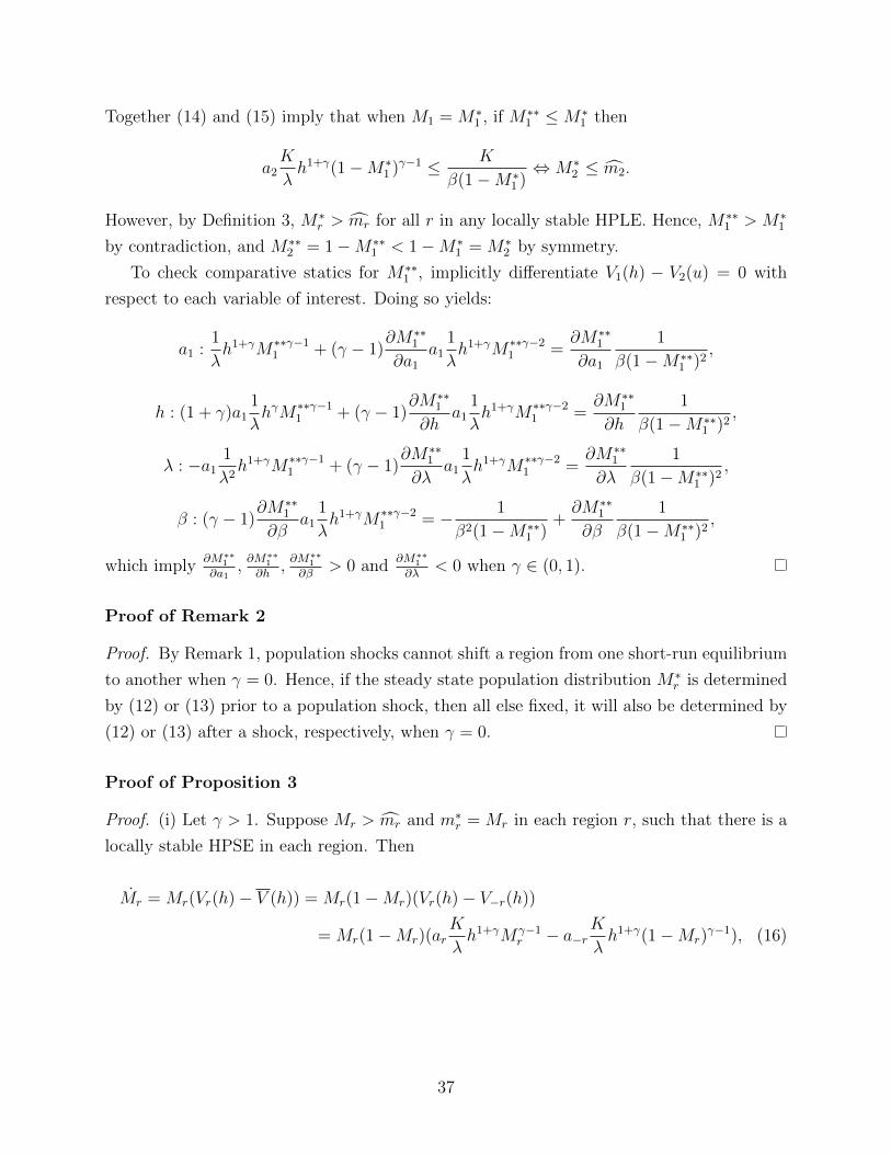
Together (14) and (15) imply that when M1 = M∗1 , if M∗∗

1 ≤M∗1 then

a2K

λh1+γ(1−M∗

1 )γ−1 ≤ K

β(1−M∗1 )⇔M∗

2 ≤ m2.

However, by Definition 3, M∗r > mr for all r in any locally stable HPLE. Hence, M∗∗

1 > M∗1

by contradiction, and M∗∗2 = 1−M∗∗

1 < 1−M∗1 = M∗

2 by symmetry.

To check comparative statics for M∗∗1 , implicitly differentiate V1(h) − V2(u) = 0 with

respect to each variable of interest. Doing so yields:

a1 :1

λh1+γM∗∗γ−1

1 + (γ − 1)∂M∗∗

1

∂a1

a11

λh1+γM∗∗γ−2

1 =∂M∗∗

1

∂a1

1

β(1−M∗∗1 )2

,

h : (1 + γ)a11

λhγM∗∗γ−1

1 + (γ − 1)∂M∗∗

1

∂ha1

1

λh1+γM∗∗γ−2

1 =∂M∗∗

1

∂h

1

β(1−M∗∗1 )2

,

λ : −a11

λ2h1+γM∗∗γ−1

1 + (γ − 1)∂M∗∗

1

∂λa1

1

λh1+γM∗∗γ−2

1 =∂M∗∗

1

∂λ

1

β(1−M∗∗1 )2

,

β : (γ − 1)∂M∗∗

1

∂βa1

1

λh1+γM∗∗γ−2

1 = − 1

β2(1−M∗∗1 )

+∂M∗∗

1

∂β

1

β(1−M∗∗1 )2

,

which imply∂M∗∗

1

∂a1,∂M∗∗

1

∂h,∂M∗∗

1

∂β> 0 and

∂M∗∗1

∂λ< 0 when γ ∈ (0, 1).

Proof of Remark 2

Proof. By Remark 1, population shocks cannot shift a region from one short-run equilibrium

to another when γ = 0. Hence, if the steady state population distribution M∗r is determined

by (12) or (13) prior to a population shock, then all else fixed, it will also be determined by

(12) or (13) after a shock, respectively, when γ = 0.

Proof of Proposition 3

Proof. (i) Let γ > 1. Suppose Mr > mr and m∗r = Mr in each region r, such that there is a

locally stable HPSE in each region. Then

Mr = Mr(Vr(h)− V (h)) = Mr(1−Mr)(Vr(h)− V−r(h))

= Mr(1−Mr)(arK

λh1+γMγ−1

r − a−rK

λh1+γ(1−Mr)

γ−1), (16)

37

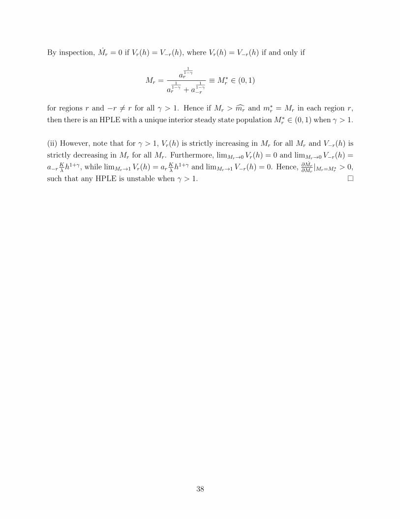
By inspection, Mr = 0 if Vr(h) = V−r(h), where Vr(h) = V−r(h) if and only if

Mr =a

11−γr

a1

1−γr + a

11−γ−r

≡M∗r ∈ (0, 1)

for regions r and −r 6= r for all γ > 1. Hence if Mr > mr and m∗r = Mr in each region r,

then there is an HPLE with a unique interior steady state population M∗r ∈ (0, 1) when γ > 1.

(ii) However, note that for γ > 1, Vr(h) is strictly increasing in Mr for all Mr and V−r(h) is

strictly decreasing in Mr for all Mr. Furthermore, limMr→0 Vr(h) = 0 and limMr→0 V−r(h) =

a−rKλh1+γ, while limMr→1 Vr(h) = ar

Kλh1+γ and limMr→1 V−r(h) = 0. Hence, ∂Mr

∂Mr|Mr=M∗

r> 0,

such that any HPLE is unstable when γ > 1.

38