Shiv Shankar Vembadi - era.library.ualberta.ca · model is first identified using downhole temperature and well rate data. ... ii Acknowledgements ... Intelligent well completion

Real-Time Feedback Control of the SAGD Process using Model Predictive

Control to Improve Recovery: A Simulation Study

by

Shiv Shankar Vembadi

A thesis submitted in partial fulfillment of the requirements for the degree of

Master of Science

in

Petroleum Engineering

Department of Civil and Environmental Engineering

University of Alberta

© Shiv Shankar Vembadi, 2014

ii

Abstract

Scope of the Work: For over a decade, the oil industry has been moving to “smart

fields”, which deploy wells with remotely operated valves and permanently

installed downhole sensors for real-time pressure and temperature measurements.

Real-time data from these “intelligent wells” provide key knowledge about the

reservoir performance and enable continuous and automatic production

optimization for better economics. In this study, we apply intelligent wells with

fiber-optic array temperature sensing to Steam Assisted Gravity Drainage

(SAGD) for real-time production optimization using Model Predictive Control

(MPC), which is a multivariable constrained control strategy. A linear empirical

model is first identified using downhole temperature and well rate data. Based on

the linear model and real-time temperature and rate data, an MPC controller

manipulates the well rates to control the subcool along a well pair in a SAGD

reservoir. We use a multilevel control framework, in which the well settings from

long-term optimization using a reservoir model provide the “set points” for MPC.

Procedure: To evaluate the use of MPC for real-time control of subcool in

SAGD, we use three-dimensional heterogeneous reservoir models with a single

pair of dual tubing string horizontal wells. A set of porosity and permeability

realizations are created. Two realizations are selected to represent two different

cases of uncertain reservoir models. Further, another realization is created that is

considered as the “synthetic” (virtual) reservoir. For each of the two reservoir

iii

models, a proprietary reservoir simulator is used to find the optimum rates and

subcool. Then MPC is used to control the subcool along the well pair in synthetic

reservoir.

Results, Observations and Conclusions: Using the multilevel control framework,

NPV improves by 18.23% and 8.81% in the two cases of reservoir models, over a

direct application of the optimum rates. Though the results validate the use of

MPC for real-time optimization of SAGD, we faced a couple of issues (which

have related practical concerns) in the identification of good linear models and

subsequently using them in the MPC controller because of steam breakthrough in

the dual tubing string well pair. However, we conclude that identification of good

linear models will be feasible if ICVs are used in the injector and producer, which

allow for more uniform steam distribution in the injector and differential steam

trap control in the producer.

Work’s Novelty: A few other works present results for the use of proportional-

integral-derivative (PID) control for automatic feedback control of the SAGD

variables. However, unlike the MPC strategy, the PID-control strategy is a single-

input and single-output control strategy. It acts on each controlled variable in

isolation by manipulating a single variable instead of optimizing the whole system

as the MPC strategy does.

iv

“What we see depends mainly on what we look for.” – John Lubbock

“Science is a way of thinking much more than it is a body of knowledge.” – Carl

Sagan

To My Father

who encouraged me to look for the right things, be curious about the world

around me and have a skeptical inclination.

v

Acknowledgements

I would like to sincerely thank my supervisors, Dr. Japan Trivedi and Dr. Vinay

Prasad, who gave me an opportunity to pursue a Master of Science degree at the

University of Alberta under their guidance. Throughout my degree program, they

corrected me whenever I was faltering in my research, in technical matters or

otherwise, and motivated me whenever I displayed a lack of confidence in myself

to accomplish the goals of this research. They have also been very understanding.

On a number of occasions, I dragged the meetings very long by engaging in

intense discussions on various technical or practical aspects of the research, and

tested their patience, but they were still very kind. I have all to thank them for.

With an undergraduate degree in Petroleum Engineering, conceptually the most

difficult part in this research was understanding the process control part of it and

relating it to intelligent oil fields. I want to thank Dr. Vinay for bearing with me

for the hard time I gave him through incessant clarifications and questions on this

part of the research. As a result of all those discussions, I now feel I have a good

basic understanding of this area, with a unique opportunity to augment it further

as I go along in my oil and gas career.

I would like to mention that on the behest of Dr. Japan, Computer Modelling

Group Ltd. arranged for an individual license for us, for their optimization and

simulation products, which was essential to finish this work in time.

vi

Table of Contents

Abstract .................................................................................................................. ii

Acknowledgements ............................................................................................... v

Table of Contents ................................................................................................. vi

List of Tables ...................................................................................................... viii

List of Figures ....................................................................................................... ix

List of Abbreviations ......................................................................................... xiv

1. Introduction ....................................................................................................... 1

1.1. Decision-Making Levels in Reservoir Management ................................... 2

1.2. Smart Fields for Production Optimization ................................................... 4

1.3. Controlling the SAGD Process .................................................................... 7

1.3.1. Steam Trap for Production Control: Optimum Subcool ....................... 8

1.3.2. Heterogeneous Steam Chamber Growth: Reasons and Implications.. 10

1.3.3. Technologies to Offset Non-Uniform Steam Chamber Growth ......... 13

1.4. Hypothesis ................................................................................................. 25

1.4.1. Research Questions ............................................................................. 28

1.4.2. Relation to Other Works on SAGD Well Control .............................. 28

1.5. Thesis Outline ............................................................................................ 33

2. Model Predictive Control ............................................................................... 35

2.1. Outline of MPC .......................................................................................... 36

2.2. MPC Optimization Problem ...................................................................... 40

2.3. Controller Design Considerations .............................................................. 42

3. System Identification ...................................................................................... 44

3.1. Stochastic Processes in Real-World Applications ..................................... 48

3.2. Overview of System identification ............................................................ 55

vii

3.3. Difference Equation Model Structures ...................................................... 57

3.4. Identification of MIMO Models ................................................................ 64

3.5. Optimal Predictor ....................................................................................... 66

3.6. Input Excitation for Identification ............................................................. 72

4. Simulation Study: Models and Procedure .................................................... 77

4.1. Numerical Models ...................................................................................... 77

4.2. Well Configuration and Modeling ............................................................. 83

4.3. Model-Based Optimization of Well Rates ................................................. 84

4.4. Economic Parameters for Optimization ..................................................... 89

4.5. Interwell Subcool Control .......................................................................... 92

5. Results ............................................................................................................ 115

6. Discussion, Conclusions and Recommendation for Future Work ........... 130

6.1. Discussion ................................................................................................ 130

6.2. Conclusions .............................................................................................. 139

6.3. Recommendation for Future Work .......................................................... 141

Bibliography ...................................................................................................... 142

viii

List of Tables

Table 3.1: Description of polynomials in difference equation model structures. 65

Table 4.1: Fluid and Rock Properties used in simulation models. 79

Table 4.2: Well dimensions used in our simulation study. 84

Table 4.3: Candidate values for optimization using P10 reservoir model. Optimum

values found by CMOST are underlined. 88


values found by CMOST are underlined. 89

Table 4.5: Identification and control periods. Any differences in the P80 case are

noted. 96

Table 4.6: Model gains in °C/m3/d for the heel subcool and toe subcool models

identified in first and second identification periods from the data recorded

from trial simulations of synthetic reservoir. 106

Table 4.7: Time constants and settling times for the heel subcool and toe subcool

models identified in the trial simulations of synthetic reservoir. 108

Table 5.1: NPV, cumulative oil production and cSOR statistics for the total

identification and control period, first identification plus control period and

second identification plus control period in the P10 reservoir model case. 116


identification and control period, first identification plus control period and

second identification plus control period in the P80 reservoir model case. 120

ix

List of Figures

Fig. 1.1: Steam chamber in crosswell plane in SAGD. 8

Fig. 1.2: a) Map (left) of steam chamber depth along SAGD wells interpreted

from 4D seismic (Suncor 2013); b) Varying subcool along horizontal SAGD

wells. 11

Fig. 1.3: An artificially lifted dual tubing string producer used by ConocoPhillips

at its oil sands project in Surmont (ConocoPhillips 2008). 13

Fig. 1.4: Intelligent well completion tested in Orion field (Clark et al. 2010). The

diagram shows steam diverters, ICVs, ICV control lines and downhole

instrumentation. 20

Fig. 1.5: Seismic thermal map (top), DTS temperature profile and steam

injectivities (bottom) for the trial well pair in Orion field (Clark et al. 2010).

Heel region (intervals A and B) shows little steam chamber growth. 23

Fig. 1.6: Multilevel oilfield management framework for real-time operations.

Saputelli et al. (2003) expound on the multilevel framework. 27

Fig. 1.7: Temperature maps showing steam chamber development in the vertical

plane containing a SAGD well pair, in the base case (left), which uses a

constant injection pressure with the wells modeled as line sources, and PID-

control case, which uses ICVs, at 12 (top), 18 (middle) and 24 months in

Gotawala and Gates (2009). 31

Fig. 2.1: MPC of a single-input single-output system. Adapted from Seborg et al.

(2004). 39

Fig. 2.2: Schematic diagram of MPC of subcool in SAGD. 40

Fig. 3.1: Dynamic behavior of a first-order system. 46

Fig. 3.2: Effect of stochastic processes on the measured output in a process. 55

x

Fig. 3.3: General difference equation model structure in system identification. 58

Fig. 3.4: The ARX model. 60

Fig. 3.5: Example of an RBS signal. 75

Fig. 4.1: NPV histogram for the 100 realizations used to select P10 and P80

reservoir models. 81

Fig. 4.2: J-K cross section of P10 reservoir model containing the wells. The map

shows I-direction permeability values of the grid blocks in millidarcies. 81

Fig. 4.3: The P10 reservoir model showing the I-direction permeability values. 82

Fig. 4.4: Optimum steam injection pressures in 13 time intervals for the 2D model

used in Gates and Chakrabarty (2006). 87

Fig. 4.5: Evolution of objective function (in dollars) in CMOST for the P10

reservoir model. Objective function value is plotted along y-axis, and job

number is along x-axis. 91

Fig. 4.6: Evolution of objective function (in dollars) in CMOST for the P80

reservoir model. Objective function value is plotted along y-axis, and job

number is along x-axis. 92

Fig. 4.7: A schematic representation of the MATLAB workflow used for

identifying linear models and controlling the SAGD wells in synthetic

reservoir. 94

Fig. 4.8: Simulation performance of models identified for heel subcool (top) and

toe subcool, represented by a dashed line, against data recorded from a trial

simulation of synthetic reservoir, for the first identification plus control

period. 100


toe subcool, represented by a dashed line, against data recorded from a trial

simulation of synthetic reservoir, for the second identification plus control

period. 101

xi

Fig. 4.10: Heel (top) and toe injection rates used for the first identification plus

control period in the trial simulation of synthetic reservoir corresponding to

Fig. 4.8. 102

Fig. 4.11: Heel (top) and toe oil rates used for the first identification plus control

period in the trial simulation of synthetic reservoir corresponding to Fig. 4.8.

103

Fig. 4.12: Simulation performance of ARX model for heel subcool, represented

by a dashed line, against data recorded from the trial simulation of synthetic

reservoir corresponding to Fig. 4.8, for the first identification plus control

period. 104

Fig. 4.13: Simulation performance of ARX model for heel subcool, represented

by a dashed line, against data recorded from the trial simulation of synthetic

reservoir corresponding to Fig. 4.9, for the second identification plus control

period. 104

Fig. 4.14: 20-step prediction performance of the model identified for heel subcool,

represented by a dashed line, against data recorded from the trial simulation

of synthetic reservoir corresponding to Fig. 4.8, for the first identification

plus control period. 107


represented by a dashed line, against data recorded from the trial simulation

of synthetic reservoir corresponding to Fig. 4.9, for the second identification

plus control period. 107


toe subcool, represented by a dashed line, against data recorded from the trial

simulation of synthetic reservoir corresponding to Fig. 4.8, for the first

identification plus control period. To identify the models, RBS signals were

used in the synthetic reservoir that had a bandwidth that was one-fifth the

xii

recommended amount. Other things, including the sampling interval, remain

the same as the models in Fig. 4.8. 110

Fig. 4.17: 20-step (top) and 60-step prediction performance of the model

identified for toe subcool, represented by a dashed line, against data recorded

from the trial simulation of synthetic reservoir corresponding to Fig. 4.8, for

the first identification plus control period. 112

Fig. 5.1: Comparison of heel (top) and toe injection rates with MPC and without

MPC in the P10 reservoir model case. 117

Fig. 5.2: Comparison of heel (top) and toe oil rates with MPC and without MPC

in the P10 reservoir model case. 118

Fig. 5.3: Comparison of heel (top) and toe subcool with MPC and without MPC in

the P10 reservoir model case. MPC tracks the set points. 119


MPC in the P80 reservoir model case. 121


in the P80 reservoir model case. 122


the P80 reservoir model case. MPC tracks the set points. 123


MPC in the P10 reservoir model case when linear models are identified using

only 2 months of input-output data. 126


in the P10 reservoir model case when linear models are identified using only

2 months of input-output data. 127


the P10 reservoir model case when linear models are identified using only 2

months of input-output data. MPC tracks the set points. 128

xiii

Fig. 6.1a: Reservoir steam chamber shape on 01-01-2014 (365 days), before the

start of first identification period, when with MPC and without MPC cases

are the same. 132

Fig. 6.1b: Reservoir steam chamber shape without MPC (top) and with MPC on

01-01-2016 (1095 days) in the P10 reservoir model case. The temperatures

of white cells lie below the range of the temperature scale. 133

Fig. 6.1c: Reservoir steam chamber shape without MPC (top) and with MPC on



Fig. 6.1d: Reservoir steam chamber shape without MPC (top) and with MPC on



Fig. 6.2a: Temperature profile, with MPC and without MPC, in the synthetic

reservoir in the P10 case on 01-01-2016 (1095 days) in the range of blocks in

well plane in the layer k = 5, which lies in between the wells, from j = 16 to

j = 55. 137

Fig. 6.2b: Temperature profile, with MPC and without MPC, in the synthetic



j = 55. 137

Fig. 6.2c: Temperature profile, with MPC and without MPC, in the synthetic



j = 55. 138

xiv

List of Abbreviations

Abbreviations:

2D two-dimensional

3D three-dimensional

ARIX autoregressive integrated with exogenous input

ARX autoregressive with exogenous input

ATS array temperature sensing

BJ box-jenkins

cSOR cumulative steam/oil ratio

CWE cold water equivalent

DTS distributed temperature sensing

GUI graphical user interface

FIR finite impulse response

ICD inflow control device

ICV interval control valve

LTI linear time invariant

MPC model predictive control

NPV net present value

OCD outflow control device

ODE ordinary differential equation

xv

pdf probability distribution function

PID proportional-integral-derivative

RBS random binary signal

SAGD steam assisted gravity drainage

SCADA supervisory control and data acquisition

SOR steam/oil ratio

STL stock tank liquid

1

1. Introduction

In this chapter, we will first consider the challenge in reservoir management of

integrated decision making at different time scales. In practice, while the reservoir

models are used for overall field development and production planning, the short-

term well operating points that are used often disregard the long-term field

performance needs. The reason is outlined. However, as digital data takes the

center stage in oil fields with the use of smart-field technologies, it has enabled

enhanced production control and integrated operations. Additionally, through the

use of integrated software tools and field controllers, there exists an exciting

possibility of implementation of field-wide production optimization in real time—

by making use of the real-time data in smart fields. Till now, optimization efforts

in oil fields have only been independently focusing on different elements of the

production system without a field-wide optimization framework.

We will then discuss Steam Assisted Gravity Drainage (SAGD), which forms the

focus of this work. SAGD is a low pressure oil recovery process that uses long

horizontal wells for steam injection and oil production. The main challenge in the

process is to develop a uniform steam chamber, upon which the oil recovery and

the process efficiency hinge. Different technologies, including smart-field

technologies, have been used to control the steam chamber formation.

Finally, in the context of the SAGD process, we will consider a multilevel control

and optimization framework for real-time feedback control of the process while

integrating the long-term production plans from the reservoir models. For the

multilevel control, the model predictive control (MPC) strategy is used. Further,

in this research a data-driven modelling approach is taken for the real-time

production optimization, as data-driven models are well suited for using the high-

frequency data in smart fields to make decisions in real-time.

2

We will frame a hypothesis for this research and state the specific questions that

we aim to answer.

1.1. Decision-Making Levels in Reservoir Management

Reservoir management involves the difficult task of addressing conflicting short-

term and long-term needs, corresponding to decision-making at different time

scales. Long-term decisions (field development planning) include a consideration

of the market forces, drainage strategies to be used and infrastructure

development. In the mid-term, decisions on production and injection rates and

drilling of wells are taken. Short-term decision-making, usually referred to as

production optimization in literature, consists of activities related to fine tune well

operating points, like decline curve analysis, well tests, well rate allocation and

gas lift rate allocation. Saputelli et al. (2005), Nikolaou et al. (2006) and Foss and

Jensen (2011) describe these different levels, albeit in slightly different ways.

Seldom decisions at these different time scales are made in an integrated manner.

Numerical reservoir simulation has become the central tool in reservoir

management. Simulation models have grown very complex and large over the

years as more complex reservoirs are being developed and there is a need for

more accurate forecasts. The forecasts are used to decide well rates in the

medium-term for the highest recovery factors or the best production economics.

However, due to the inherent uncertainty in several parameters used in reservoir

models and the presence of geological features below model resolution, reservoir

performance will vary from that predicted using a reservoir model. E.g.,

uncertainty in locations and extent of fine-scale geological features like high or

low permeability layers and shale barriers, fault intensities and level of

heterogeneity can lead to uneven injection and earlier than expected water

breakthrough in waterflooding. In order to manage the uncertainty, reservoir

models can be updated regularly using history matching to fit past production

3

data. Closed-loop Reservoir Management (CLRM) has been proposed by different

authors. It includes regular and sequential implementation of model-based

optimization and history matching. Model-based optimization optimizes well

rates or pressures at multiple points of the reservoir life by maximizing or

minimizing an economic objective function. Further, to quantify the uncertainty,

the optimization exercise can use several realizations to represent the reservoir

(robust optimization) and include a risk aversion term in the objective function for

optimization. Jansen et al. (2009) do a thorough review of CLRM and illustrate

the concept. Van den Hof (2012) is a more recent work that discusses the scope

and challenges of CLRM. The works on CLRM show that significant economic

benefits can be obtained from the use of these models to optimize production and

injection plans. Though there is no case of CLRM being applied in a field,

individual elements of it are being rapidly applied.

Because of the inherent uncertainty in and distrust of reservoir model predictions,

short-term production control in fields has been largely focused on maximizing

short-term returns without any ultimate recovery considerations. The work of

Naus et al. (2006) is an example of such a production strategy. However, with the

implementation of CLRM to mitigate the uncertainty, the scope of short-term

production control can be limited by the reservoir model predictions to avoid

overlooking long-term gains. It needs to be noted that even with CLRM, short-

term optimization is necessary because different physical constraints need to be

managed (e.g., total gas lift gas available). Also, even the history matched models

in CLRM can have a large uncertainty in them; Dilib and Jackson (2012) cite

some works as examples. History matching may also take up to a year, by which

time there is more production data available. Foss and Jensen (2011) describe the

adverse effect of such a workflow related time delay on the performance of close-

loop reservoir management.

4

1.2. Smart Fields for Production Optimization

While full field reservoir models are limited to mid/long-term decision-making,

for little over a decade, oil industry has continuously made progress on the use of

smart-field technologies for short-term production optimization to manage

geological uncertainties, increase production from fields and improve economics.

The impetus for this comes from the end of “easy oil”. Fields being developed

today are increasingly complex and riskier with lower profitability. Capital and

operating expenditures are also very high coupled with a risky environment that

the oil industry field itself in today. To increase success rates, improve economics

and improve safety of the personnel, equipment and environment (especially in

deepwater drilling), operators are moving towards smart fields (discussed as the

“digital oil field”, “i-field” or “e-field”). Smart fields represent a new wave of

innovation that is changing how business is done through digitization of the

industrial world (White 2013). It is underpinned by real time data (“big data”),

low-cost remote sensing, advanced computing and improved connectivity

between the machines and their operators.

Among other applications of technology, smart fields deploy wells with

permanently installed downhole sensors and remotely operated valves. Huge

amounts of real-time data from these intelligent wells, coupled with data analytics

and domain expertise can be used to monitor the production system in real-time

(van den Berg 2007; Al-Mulhim et al. 2013). E.g., problems in wells can be

identified and well test frequency can be improved. The data can pertain to well

rates, pressures and temperatures. Further, along with collaborative work

environments (covering the reservoir, wells and production), the real-time data

makes integrated operations possible.

Apart from production monitoring, the data can be analyzed using models to

optimize the wells and field performance in real-time. Real-time Optimization

(RTO) of production system could consist of, e.g., a Supervisory Control and

5

Data Acquisition (SCADA) system to automatically gather real-time well and

surface data, analyze the data using integrated well and surface network models to

find new optimum operating points and implement the new settings in real-time.

For instance, the surface network model could be used to route wells to the

correct separator system, debottleneck the production system, optimize the gas lift

gas distribution and find the optimum well choke and separator pressure settings

(van den Berg 2007).

Different control strategies have been explored to operate the remotely operated

valves in intelligent wells for production optimization. The intelligent-well valves

provide a greater degree of production control by controlling the inflow from

different zones and enabling the continuous adjustment of well operating points.

E.g., Naus et al. (2006) maximize daily oil rates in a compartmentalized reservoir

by calculating new Inflow Control Valve (ICV) settings using a steady-state

wellbore model. The wellbore model includes inflow models for the ICV zones

and uses a choke model to represent the ICVs. Every optimization interval,

derivative information for relating a change in phase flow rates to a change in

ICV setting is re-calculated and an objective function is optimized using

Sequential Linear Programming. In this control strategy, the inflow models can

be periodically updated based on downhole pressure and temperature

measurements—such indirect estimation is called soft-sensing—combined with

regular production tests. The models should be updated when the predicted flow

rates and pressures show deviations from the measured values. Dilib and Jackson

(2012) employ a simple direct feedback control to choke the ICVs based on

downhole multiphase flow measurements. The control strategy is reactive as

valve settings are changed only in response to changes in water cut

measurements. (On the other hand, the control strategy used by Naus et al. (2006)

is proactive as it is based on future output predictions.) The authors however

conclude that even such a simple closed-loop strategy can give close-to-optimum

economic gains.

6

We refer to Saputelli et al. (2003) for a concrete definition of the nature of RTO

activities. RTO consists of continuously traversing a loop of measurement of data,

its analysis using models to calculate new operating points by solving an objective

function and lastly control, all executed at the same frequency. Real time is

therefore in reference to a certain time scale, which is the longest affordable time

between measurement of data and control. E.g., the time scale for RTO of

production is much shorter than that for mid-term planning in reservoir

management. Saputelli et al. (2003) also pointed out that (as of the writing of their

paper) RTO was used in the oil industry merely as a slogan rather than to describe

optimization in real time, if there is any optimization at all. In the industry,

optimization has been extensively applied to individual parts of the production

system. E.g., several works have focused on gas allocation in gas-lift fields. But in

these efforts, models have been used for offline optimization once rather than

automatic process control using wellhead and field controllers. The authors

outline reasons for the slow uptake of real-time production optimization, which

includes the need for further development of software tools for data acquisition

and control, and further integration in intelligent oil field.

The industry continues to make strides in moving towards this data-centric way of

producing oil fields, as a lot of the digital data accumulated from intelligent

hardware still remains unused, some even directly thrown away (Perrons and

Jensen 2014). The basis of our work is the use of integrated software tools for

real-time (hourly–daily) feedback-based optimization of well operating points

through a data-driven modelling approach and a multivariable control strategy

(MPC). Such automatic feedback control is standard in process control for plant

wide optimization, which we explain in Chap. 2.

7

1.3. Controlling the SAGD Process

With more than a decade of experience, SAGD is a mature process which is

commercially used for in-situ recovery of the bitumen reserves of Alberta. It

continues to evolve as new technologies are being developed, put into trial and

implemented, which focus on improving the efficiency of the process and the oil

recoveries. These technologies encompass Interval Control Valves (ICVs), fiber-

optic based downhole pressure and temperature measurements, gathering of

seismic data for revealing heated zones and real-time optimization of well pads.

The process involves a pair of horizontal wells at the bottom of the reservoir, with

steam injected from the top well and oil and steam condensate produced from the

bottom well. Steam rising from the injector transfers its latent heat to bitumen and

forms an expanding steam chamber with oil and condensate flowing down the

sides of the chamber to a liquid pool at the bottom of the chamber. Fig. 1.1 shows

an expanding steam chamber in crosswell plane. The dominating heat transfer

mechanism is convection in the upper part of the steam chamber (Ito and Suzuki

1999). The steam condensate flowing along the walls displaces oil far ahead of

the steam chamber through convective effects. In their analysis, Ito and Suzuki

(1999) found peak oil flow appearing as deep as 8 m ahead of the steam chamber

interface near the bottom of the reservoir. However, near the production liner,

conduction is the mean heat transfer mechanism.

8

Fig. 1.1: Steam chamber in crosswell plane in SAGD.

1.3.1. Steam Trap for Production Control: Optimum Subcool

To avoid directly drawing steam into the producer in SAGD, the level of the

liquid pool needs to be above the producer. This can be ensured by controlling the

production temperature such that it’s below the steam saturation temperature.

Roger Butler was one of the earliest to draw an analogy between controlling

SAGD wells this way and the thermodynamic steam trap used in refineries and

process industry (Edmunds 2000). For production control by steam trap, there is a

question of what an optimum interwell subcool, which is defined as the difference

in the temperatures of the injector and the producer, is. As the liquid level drops

between the injector and producer, the interwell subcool decreases. When there is

no liquid accumulation above the producer, steam breaks through at the producer

instead of expanding the steam chamber by heating more bitumen, and the

interwell subcool is zero.

SAGD economics depends more than anything on steam utilization, and hence,

the operational design focusses on the reduction of cumulative steam/oil ratio

(cSOR) over the life of a project. Edmunds and Chhina (2001) performed a series

of simulations to analyze the supply (capital and operating) costs for different

values of a constant operating steam chamber pressure and varying reservoir

quality while the producer was constrained to produce a negligible amount of

9

steam (zero subcool). They found cSOR to be a monotonic function of the

constant operating steam chamber pressure. A higher constant pressure reduces

the number of wells and increases the oil rates, but on the down side, increases the

cSOR and the supply costs due to steam. Since steam supply costs due to surface

facilities required for treating, boiling, recycling and disposing off water, and fuel

costs account for more than half of supply costs, with wells being only

responsible for 20 to 30 %, optimization of SAGD lays more emphasis on

reducing the pressure and minimizing cSOR rather than on maximizing the oil

rates. A poorer quality reservoir and higher gas price further pushes the optimum

pressure and cSOR downward. Edmunds and Chhina (2001) found that the range

of pressures that minimized the supply costs in their cases was as low as 400–750

kPaa.

Hence, for the two-dimensional (2D) illustration in Fig. 1.1, an optimum subcool

will reduce the cSOR and maintain a liquid level a little above the producer.

Based on the discussion above, the optimum subcool will be a little lower than the

value at which the cSOR is minimized. A further lower subcool ends up drawing

too much steam from the injector, which mixes with cooler fluids and condenses

before reaching the producer. This decreases the thermal efficiency of the process.

On the other hand, a higher than optimum subcool raises the liquid level present

above the producer and decreases the oil rate. The delay in oil production leads to

slower returns. Additionally, a very high liquid level also reduces the thermal

efficiency of the process as some of the latent heat of steam goes towards keeping

the oil pool at bottom hot. A range of values from 5 to 40°C has been stated in the

literature for optimum subcool. Edmunds (2000) concluded that 20–30 °C

subcool was optimum for their 2D model. In their SAGD simulation study of

McMurray formation in Hangingstone oil sands area, Ito and Suzuki (1999) found

30–40°C subcool to be the optimum based on minimization of cSOR. Gonzalez et

al. (2012) state that in practice, 15–30°C subcool is maintained between the

10

injector and producer. Optimum subcool will vary depending on the rock and

fluid properties.

1.3.2. Heterogeneous Steam Chamber Growth: Reasons and Implications

The 2D analysis in previous section notwithstanding, SAGD well-pair operation

is much more complicated in practice. As shown in Fig. 1.2, subcool varies along

the long wells used in SAGD. Edmunds (2000) showed that optimum subcool

determined from 2D simulation is overly optimistic about oil rates and cSOR.

With the combined production stream at the presumed low optimum subcool from

2D analysis, some sections of the well can draw in a lot of steam, while other

sections are cooler than the optimum. Gates and Leskiw (2008) did a simulation

study using a detailed upscaled geological model of an Athabasca oil sands

reservoir in an area near Surmont. Injecting steam at a constant pressure, they

used different constant liquid production rate constraints in different simulation

runs to note the local subcool values along the well for the simulation period. For

the highest production rate that they used that successfully prevented major steam

trap failure along the well pair, the local subcool at several intervals was above

60°C for most of the simulation period. Hence, compared to the analysis in

Section 1.3.1, defining the optimum operating conditions in SAGD has an added

layer of complexity of considering the varying conditions along the well pair.

Both steam injection and production get limited by the section of the well pair that

is most prone to steam breakthrough. This results in lower oil rates and thermal

efficiency compared to a scenario in which the steam chamber develops more

uniformly. As we will discuss in Section 1.3.3, dividing the wells into a number

of intervals (in which the steam injection and production can be individually

controlled) through the use of an intelligent completion provides a solution.

11

Fig. 1.2: a) Map (left) of steam chamber depth along SAGD wells interpreted from

4D seismic (Suncor 2013); b) Varying subcool along horizontal SAGD wells.

There are several reasons for a heterogeneous steam chamber development. These

include heterogeneous porosity, permeability, fluid saturations and oil

composition distribution around the wells. Presence of shale and mud layers near

the well pair particularly skews the steam chamber. SAGD is known to be

susceptible to these heterogeneous conditions due to a combination of high

permeability of oil sands, high mobility ratio of steam and the viscosity-

temperature relationship of bitumen. Even for two well pairs separated by 100 m,

heterogeneity can create very different steam conformance results (Gotawala and

Gates 2012). It results in varying injectivities along the well pair, because of

which steam will enter into the reservoir preferentially at certain intervals leading

to lower subcool, higher temperatures near wellbore and a larger steam chamber

size compared to other intervals. There are two such intervals in the illustration of

a SAGD well pair in Fig. 1.2. Also, the horizontal sections are drilled within

12

certain tolerances. Variations in the injector-producer distance create

heterogeneous conditions.

Even with an ideally uniform geology and interwell spacing, wellbore flow effects

will ensure non-uniform steam flow. In a simple SAGD injector well

configuration, steam travels through a tubing string landed at the toe, and the

annulus, and through the slotted liner into the reservoir. In this configuration, the

steam flow is predominantly through the annulus, and there is a significant

pressure drop and a decrease in steam quality from the heel to toe. Because of

steam’s low density and high flow rates, pressure drop in the injector dominates

over that in the producer with a high pressure differential at the heel and low

values near the toe (Edmunds and Gittins 1993). This pressure drop gets

impressed on the reservoir. Parallel flow in the reservoir can’t counteract this

pressure difference because reservoir transmissibility is only a fraction of the

wellbore flow capacities. This leads to a much faster growing steam chamber and

a low subcool at the heel whereas a stunted steam chamber and a much higher

than desired subcool at the toe. The net result is that the operator is unable to

deliver as much steam as desired into the reservoir (because of the risks of steam

breakthrough at the heel), a higher cSOR and lower oil rates due to a non-uniform

steam chamber. Many operators in Alberta use a dual tubing string inside a slotted

liner as shown in Fig. 1.3, with one tubing string landed near the heel and one

near the toe of the well, to even out the steam chamber growth (Stone et al. 2014).

Even with this configuration, a less than ideal barbell shape steam chamber forms,

as illustrated by Bedry and Shaw (2012).

13

Fig. 1.3: An artificially lifted dual tubing string producer used by ConocoPhillips at

its oil sands project in Surmont (ConocoPhillips 2008).

1.3.3. Technologies to Offset Non-Uniform Steam Chamber Growth

In wells with a dual tubing string configuration, the short- or long-tubing string

injection and production rates can be decreased in order to control undesired

steam chamber growth in some areas. However, this provides limited control over

steam placement along the well and steam chamber growth. And with longer

wells and more heterogeneity, steam conformance becomes worse.

Different technologies have been used or put on trial to diagnose and control

injection conformance and production along SAGD well pairs to counterbalance

the adverse effects of heterogeneity (Clark et al. 2010; Gotawala and Gates 2012).

These include limited entry perforations (LEPs), inflow and outflow control

devices (ICDs and OCDs), ICVs and downhole instrumentation. LEPs have been

used by operators to create a more uniform steam injection profile by generating

14

supersonic flow conditions as steam flows through a limited number of downhole

chokes into the reservoir. Under these flow conditions, the rate depends only on

upstream pressure in the well. Hence, reservoir heterogeneity doesn’t affect steam

placement as much in the case of flow through a slotted liner. A major

disadvantage with LEPs is that later in production, the flow rates will become

subsonic and the flow rate will depend on the downstream pressure in the

reservoir, bringing heterogeneity back into play.

A more complex completion technology that has been used to control the

injection/production profiles along wells in SAGD is the inflow and outflow

control devices (ICDs and OCDs). (There are variations in the name used for

these, e.g., flow control device.) These devices are deployed along the well and

work by creating a pressure drop in the fluid flowing in or out through these

devices. Through different pressure drops across these devices at different points

along the well length, the flow profile can be improved. Two different geometries

of these devices are the nozzle type and the helical or baffled pathway type. In the

former, a pressure drop is created by forcing the fluid to pass through a

constriction before it enters the tubular. In the helical or baffled pathway type, the

pressure drop is created through friction instead as the fluid is made to flow

through long channels. A still different category of ICDs is the so-called

autonomous ICDs. The pressure drop in these ICDs depends on the composition

of fluid flowing in, and hence, these devices can adapt to changing flowing

conditions. E.g., one model for autonomous ICDs is called the hybrid-geometry

autonomous ICDs, which combines flow through a baffled pathway with a series

of constrictions present along it as well. The flow pathways in autonomous ICDs

are designed so that there is more resistance to flow of water/gas compared to oil.

Hence, they can create a more uniform inflow conditions along the producer and

prevent steam breakthrough in some intervals in SAGD. Banerjee et al. (2013)

discuss the different geometries of ICDs/OCDs, the role of pressure drop through

these devices in promoting a more uniform injection and production profile as

15

well as designing of these devices. They explain that using OCDs in the injector

immediately improves the injection conformance compared to the use of a slotted

liner. Along with the OCDs in injector, using ICDs in the producer has a

“synergistic effect” as it helps create a uniform liquid level above the producer

and prevents direct inflow of steam from the producer at any point, leading to a

better cSOR as well as higher oil production. These devices can be deployed

either in the tubing string or in the liner string. In the former case, a single tubing

string containing a few of these flow control devices runs till the toe end of the

well. Since only a single tubing string is used compared to a dual tubing string in

a slotted liner, using ICDs/OCDs has the added advantage that the liner size is

smaller and consequently, so are the casing sizes. And due to the considerations in

drilling a smaller wellbore, this enables drilling longer wells. A second option is

to deploy the ICDs/OCDs in the liner string. The liner string will then consist of

some blank pipes with the rest of the length being made up by the flow devices,

equally spaced along the well length. In this configuration, only a heel tubing

string is required. Since the whole cross-sectional area of the liner is available to

flow, the liner size is further reduced compared to wells with tubing deployed

ICDs/OCDs. It also has a further benefit of doing away with the risk of pulling

out the tubing string along with the flow devices in case of a workover.

In SAGD, flow conditions along the well pair will change as the steam chamber

develops. The steam chamber grows bigger in certain intervals compared to

others, which needs a reduction in injection rates in these intervals to normalize

the steam conformance. ICDs/OCDs, on the other hand, are designed prior to

being run into a well according to the flow profiles along the well, estimated

based on reservoir properties, and field data (see below). Hence, a disadvantage

with using pre-fixed ICDs/OCDs is that they can’t be adjusted with changing flow

profiles along the well. Nozzle-type ICDs/OCDs that have adjustable nozzles also

exist; however, the workovers that are needed lead to significant downtime, and

there are other prohibitive safety considerations as well (Bedry and Shaw 2012).

16

Other works have focused on the use of reservoir models, with or without the

quantification of uncertainty by using multiple Geostatostical realizations, to

optimize SAGD variables (Gates and Chakrabarty 2006; Yang et al. 2009, 2011).

Yang et al. (2009) optimize injection and production rates by maximizing Net

Present Value (NPV) for a real-field three-dimensional (3D) model. Though these

optimization efforts are expected to lead to improved operations, there is a

significant uncertainty still associated with the field results due to the nature of

the SAGD process itself, as Clark et al. (2010) note for the Orion SAGD project.

Intelligent Wells

Intelligent wells with ICVs involve further infrastructure complexity and higher

capital investment, but offer the best ability to normalize steam chamber growth

and manage uncertainty in field production. An intelligent well completion for

SAGD wells would consist of a tubing string, containing a few ICVs and sealed at

the end, run to the toe inside a liner. Hydraulic control lines, clamped to the

tubing string at the tubing couplings, run alongside the whole string. The ICVs are

remotely actuated via these control lines. The valves are sliding sleeves and can

be either on/off type or multiple position type. A multiple position type ICV can

be choked in increments from a fully open position to a fully closed position.

Further, the well would be instrumented with optical fiber-based technology for

pressure and temperature measurements. The optical fibers run alongside the

tubing string inside capillary tubes. Also, for full control of injection or

production along the well length using the ICVs, the tubing string consists of

diverters placed in between the valves to isolate the annulus into several intervals.

The diverter seals against the annulus and prevents annular flow between the

intervals. For designing the diverters, the high-temperature downhole conditions

that occur in SAGD are an important factor. Unlike packers, which anchor to the

casing, the diverters need to allow tubing movement during thermal changes

without compromising the seal with liner. Diverter elements should allow the

17

hydraulic control line and capillary tubes to pass through them while at the same

time maintaining the seal with the liner. The ICVs, hydraulic control fluid,

downhole instrumentation and diverters all need to be designed so that they can

withstand the high temperatures encountered in SAGD.

While ICDs/OCDs are passive devices, ICVs are active control devices. They

allow the injection profiles to be changed throughout the life of the well pair.

Further, the use of ICVs along with the zonal isolation achieved using diverters

enables differential steam trap control to individually maintain a liquid level

above the producer in all the intervals throughout production. Hence, using ICVs

has the dual benefit of improved steam conformance and differential steam trap

control, which improves cSOR and increases oil production rates.

Two fiber-optic technologies for downhole pressure and temperature

measurements are the fiber-optic pressure and temperature gauges, and

Distributed Temperature Sensing (DTS). In the oil industry, DTS is by far the

most commonly used downhole fiber-optic monitoring technology (Jacobs 2014).

The uptake of this technology by operators has been accelerating as technological

advancements have made it reliable and durable. And as the industry moves

towards more complex and risky fields, fiber-optic monitoring technologies give

the operators confidence in developing them. The operators gain key knowledge

about the reservoir through the use of these technologies—even if deployed in a

few of the wells in a field—which helps them manage their injection and

production plans better. Also, along with remotely controlled downhole valves,

these technologies can be used in controlling flow into well segments in real-time.

The DTS system consists of a hair thin fiber-optic cable run in the well. The cable

goes to a box called the interrogator unit at the surface. The interrogator has a

laser which sends light pulses through the fiber-optic cable made of silica at rates

as high as upwards of 10,000 times a second. The light loops through the cable

and is received back by an optical receiver in the interrogator, where the optical

18

signal is converted into electronic signal and processed for noise. DTS can give

accurate temperature measurements every meter of the well. For fiber-optic

pressure and temperature gauges, a fiber-optic cable runs in the well and

terminates at the location where a gauge is mounted on the tubing string. The

temperature sensor is integrated with the pressured sensor and is meant for both

providing a temperature measurement and applying a thermal correction to the

pressure measurement. The technological advancements that have enabled wider

application of these technologies include improvements in glass chemistry that

have improved the silica fibers to be able to withstand harsh downhole

environments. In the high temperatures encountered in SAGD, an earliest problem

with the fiber-optic cables had been hydrogen darkening—we refer to Jacobs

(2014)—which soon made the interrogator unable to make useful measurements

due to distortion or darkening in the signals because of hydrogen atoms (from oil

produced) that enter into the silica fibers. The darkening increases with time and

temperature. Recently, companies that provide these monitoring technologies

have been able to mitigate and manage this problem, through both use of

chemically resistant materials in the cable and advances in laser technology,

paving the way for more widespread use of fiber-optic monitoring in SAGD.

Further, increase in computer processing speed and efficient algorithms mean that

the data from downhole fiber-optic technologies can be interpreted fast-enough

for monitoring the well conditions in real-time.

In SAGD, using data from DTS and fiber-optic pressure and temperature gauges,

we can know how conditions along the well are changing with production and

infer the steam chamber shape. These changes can be monitored in short-term and

injection and production plans accordingly modified. Temperature data from

downhole optical fibers during shut-in is a good indication of near-wellbore

temperatures (see below for a field study by Clark et al. (2010)). Near-wellbore

temperature profile reveals injection conformance and production profiles.

Pressure data from downhole pressure sensors during injection or transient

19

pressure analysis during shut-in of the injector is used to calculate injectivities in

different intervals. An interval which has high temperature and high injectivity

relative to other intervals takes a disproportionate amount of the steam injected.

This results in low total steam injectivity (due to steam breakthrough concerns)

and lower oil production rates. Also, it increases the steam chamber size in the

interval and hence, further distorts the steam injectivity along the well and

worsens steam conformance. To normalize the steam chamber, injection in these

intervals should be decreased while continuing to monitor injectivity along the

well and temperature profile.

For real-time analysis of conditions along a SAGD well pair, Gonzalez et al.

(2012) contend that an Array Temperature Sensing (ATS) fiber-optic system with

multiple temperature measurement points along the wellbore and at least one

pressure point is suitable. In comparison, DTS provides very high-resolution

temperature data less apt for real-time analysis. They describe an integrated

software tool to monitor, evaluate and control temperatures and pressures in

horizontal sections of the injector and producer (inflow of the system) as well as

monitor and optimize the artificial lift system (outflow) in real-time while

integrating information on wellhead rates and temperatures. The system is thus

used to control the subcool along the well pair by changing the injection and

production rates. For optimizing the SAGD process using the system described in

this work, temperature and pressure measurement points are needed in both

injector and producer.

Clark et al. (2010) present the design and early field results for the field trial of an

intelligent completion system in a SAGD injector in Orion field in the Cold Lake

Oil Sands Area. They state that, based on the modeling works of the likes of

Gotawala and Gates (2009), differential steam trap control using ICVs can lead to

a 5–10% increase in recovery and 20–40% reduction in cSOR depending on the

level of heterogeneity in the reservoir. In the case of Orion field, greater than

expected geological heterogeneity was leading to a variable performance between

20

the well pairs. The producer temperature data (obtained using DTS), production

performance data and seismic maps showing heated zones indicated that using

ICVs for steam conformance improvement and differential steam trap control

would improve the performance in field. It was decided to initially use an

intelligent completion in the injectors, and later a completion would also be

developed for deployment in the artificially lifted producers to achieve full

control. For the trial, they chose the injector in a well pair which had enough

baseline data for a comparison with the ICV test results later, producer equipped

with DTS, and poor cSOR and lower oil production rates compared to other well

pairs. The completion in the injector was pulled out and the intelligent well

completion shown in Fig. 1.4 was installed.

Fig. 1.4: Intelligent well completion tested in Orion field (Clark et al. 2010). The

diagram shows steam diverters, ICVs, ICV control lines and downhole

instrumentation.

The wells in the field are approximately 750 m long. Four on/off type ICVs are

used in the trial injector to divide it into four intervals: A (heel), B, C and D (toe).

The ICVs were designed and tested up to temperatures of 265°C and pressures of

21

20,600 kPa. Each ICV is attached to two hydraulic control lines. There is one

control line per ICV to open it, and a common control line closes all the ICVs,

making it a total of five control lines. Having a common control line to close all

the ICVs avoids the complexity and expense of additional control lines. With this

configuration, n ICVs require n + 1 control lines. (However, the authors note that

this control configuration soon reaches the space limitations inside the well and

wellhead if the well length is increased and more ICVs are used. For higher

number of ICVs, a “multiplexed control system” is needed.) The control lines are

connected to a manifold at the surface, and a hydraulic control panel is used to

open and close the valves. A custom designed diverter was used, which had a

special assembly that allowed the control lines and fiber-optic cables to pass

through it safely without needing to splice them. This was important for reliable

operation of DTS and considerably reduced the completion complexity and time.

In each of the intervals B, C and D, a pressure and temperature gauge is mounted

on a custom-made gauge carrier just below the ICV valve. The gauges selected

for the completion had a temperature rating of 260°C. A fiber-optic cable running

inside a capillary tube transmits pressure and temperature information from the

sensors to the surface. Pressure in interval A is measured through the nitrogen-

filled annulus. The capillary tube that carries a fiber-optic cable to interval D also

consists of a DTS system for monitoring the temperature profile along the well.

After the completion was installed, it was tested to check the functioning of the

equipment, gather data on the completion performance under steam injection

conditions and fine-tune the well operating procedures. First the downhole

instrumentation was validated. Then the well operation was tested. The test

conditions included injection with all valves closed, all valves open and only one

valve open. It was demonstrated that the ICVs functioned reliably up to pressures

of 4600 kPa and temperature close to 260°C. Diverters provided good annular

isolation under pressure differentials up to 800 kPa. Data from DTS and the

pressure and temperature gauges were critical in understanding the equipment

22

performance and well response. DTS gave good accuracy and resolution under the

testing conditions. The gauges showed good reliability and stability. The testing

phase resulted in a lot of good data for carrying out the trial of intelligent

completion.

After the well function testing, there was a further phase of testing over a month

to collect baseline data about the current steam chamber and injection profile

characteristics. Steam was injected into each of the intervals individually over a

number of days; based on the pressure data from the downhole pressure gauges

and injection rates, an injectivity index for each interval was estimated. Further,

DTS data was collected over a number of 24-hour periods after both the injector

and producer were shut in. After an initial period of rapid cooling and transient

effect during these shut-ins, the temperature profile from DTS provided a good

indication of the near-wellbore temperatures. Intervals A and B had low

injectivities and lower near-wellbore temperatures for both injector and producer,

indicating that these intervals had smaller steam chamber size and had low

production rates. On the other hand, intervals C and D had good injectivities and

higher near-wellbore temperatures. The injectivities and temperature profiles from

DTS agreed well with a seismic thermal map interpreted from 2D seismic lines

taken just before the installation of the intelligent completion in the injector.

These observations also corresponded with the geological information available: a

large fraction of the injector and producer well lengths in the heel region lied in

low vertical permeability zones.

23

Fig. 1.5: Seismic thermal map (top), DTS temperature profile and steam injectivities

(bottom) for the trial well pair in Orion field (Clark et al. 2010). Heel region (intervals

A and B) shows little steam chamber growth.

To create a more uniform steam chamber, and hence improve injection

conformance and increase the total steam injectivity in the injector, an injection

plan was formulated that aimed to selectively inject into intervals A and B. The

injection plan consisted of cycles of injection, with each cycle composed of

Three week of injection into intervals A and B.

One week of injection into all intervals.

24-hour shut-in for DTS measurements.

The intermediate injection into the whole well in each cycle was meant to keep

the toe intervals in the well pair warm, and maintain the steam chamber size in

those intervals. The authors report the well-pair performance after two cycles of

injection. After two cycles, an improvement in injectivities in intervals A and B

between 30% and 70% was seen. Pressure measurements revealed that there was

24

an increasing communication of the heel intervals with the steam chamber in the

toe intervals. Based on the shut-in DTS temperature profile, temperatures near the

injector increased by 10–20°C in the heel intervals. Temperature hadn’t yet

increased much around the producer indicating that oil production from heel

intervals hadn’t improved much. cSOR improved by 20% after just the two

cycles, while the oil production rate remained around the same, compared to the

well-pair performance a few months prior to the installation of intelligent

completion. The improvement in cSOR is likely because of the fact that there is

less steam directly flowing from the injector to the producer in the toe region. A

number of additional cycles of injection were further planned to see if ultimately

uniform steam conformance could be achieved. It was planned to continue

monitoring the well through shut-in DTS temperature profiles, changes in

injectivity and production performance of the well pair. The injection cycles could

be accordingly modified to injection periods. Further, if a significant

communication of steam injected in heel interval with the steam chamber in toe

intervals, injection be only in interval A instead of both A and B. Seismic data at

some later point would also help confirm the steam chamber growth.

According to the authors, the focus for further technology development work in

the field includes increasing the temperature rating of the ICVs and development

of multiple position ICVs, which will allow better control of injection and profiles

without having to shut in certain intervals.

Manual Well Control

In practice, using the technologies described above, wells are controlled manually

in SAGD to transfer the heat uniformly and control the steam chamber growth,

while handling constraints like steam treatment capacity and well artificial lift

constraints.

25

Manual control, however, considers relationships between the variables in

isolation instead of in an integrated manner. SAGD is a complex dynamic process

with many interacting variables. When trying to control subcool along the well

pair, based on real-time data, for uniform steam injection (and hence, better steam

conformance), subcool will depend on both injection and production rates. A

change in the injection rate changes the interwell subcool, which changes the

inflow at producer. At the same time, the inflow at producer also depends on the

outflow settings (artificial lift). Hence, both inflow and outflow relationships need

to be considered at the same time (Gonzalez et al. 2012). With manual

monitoring, it becomes more difficult to do so as the number of wells increase.

Further, changing the injection rate at, say, heel will also affect the subcool at toe,

which is coupled to the subcool at heel through the wellbore. Hence, all real-time

downhole pressure and temperature data needs to be integrated with real-time

surface production rate measurements to effectively control the process. As Patel

et al. (2014) have elaborated on, manual control of wells and management of

system constraints can be effective only in case of a few wells, up to 5–10 of

them.

Additionally, Edmunds (2000) concludes from his 2D subcool analysis that “there

is no unique, quasi–steady state solution of the steam trap problem; rather there

are only solution trajectories, whose future evolution depends not just on the

boundary conditions of the moment but all past history as well.” So, the

relationships between injection/production rates and interwell subcool are time

varying as the steam chamber grows from ramp-up to plateau to wind-down phase

in SAGD. This is a further complication for SAGD well control.

1.4. Hypothesis

Section 1.2 ends on the note that intelligent oil fields provide an opportunity for

real-time feedback-based production optimization. Section 1.3.3 discusses how

26

intelligent wells in SAGD enable better production control for a more uniform

steam chamber growth and higher recovery, but that manual control of wells

doesn’t consider all the variables and constraints of the system at the same time.

We could compare this situation with a chemical plant, where there can be

thousands of process variables, which also have inequality constraints. In such

plants, MPC, which is an advanced multivariable constrained process control

technique, is widely used for automatic feedback and feedforward control of

multiple variables while handling constraints. The hypothesis for this research

follows from this and other discussion previously:

RTO of SAGD using the data from instrumented wells will lead to significant

efficiency gains, improve recovery and mitigate uncertainty inherent in the

best reservoir model predictions. The MPC strategy is suitable for

integrating all downhole and surface real-time data for controlling the

process.

As the industry continues to make a transition to smart fields, this simulation

study aims to add to the literature by evaluating the capability of advanced

process control in optimizing production. One approach for RTO using the MPC

strategy is to use the high frequency data from downhole sensors to build simple

data-driven linear dynamic models for implementing the control strategy

(Nikolaou et al. 2006; Essen et al. 2011; Essen et al. 2013). Specifically in our

work, a simple linear model, built using regression from temperature and rate data

from wells to capture the dynamic input-output relationships, is used in the MPC

strategy to control the subcool along a SAGD well pair.

Further, to take both long-term and short-term reservoir management needs into

account, the MPC of subcool along the wells is integrated with well settings

obtained from long-term optimization done using a reservoir model, as part of a

multilevel control and optimization framework. Fig. 1.6 is a simple illustration of

the oilfield management framework we considered. Such a hierarchical

27

decomposition of operations exists in the process control industry for integrated

optimization of plant operations (Seborg et al. 2004). We refer to Saputelli et al.

(2003), who expound on the field operations hierarchy for RTO in oil fields. The

different layers in the framework shown in Fig. 1.6 have different timescales for

decision-making. The timescales are indicated in the figure. The upper layers pass

down decisions related to design and/or operations to lower levels as goals (or set

points) to be followed. At the same time, data from the lower levels are used for

feedback-based decision-making at upper levels.

Fig. 1.6: Multilevel oilfield management framework for real-time operations.

Saputelli et al. (2003) expound on the multilevel framework.

Regulatory control, which is the lowermost level in Fig. 1.6, involves direct

feedback control of individual chokes and valves to control pressures, rates and

temperatures. At the multivariable control level (MPC), a centralized SCADA

system coordinates the wells and surface network by calculating new operating

points. The operating points are calculated every few hours based on the current

data on the controlled variables (which, in our case, is the subcool along the

SAGD well pair) from well measurements, which are made every few minutes at

the regulatory level. The operating points (pressures and rates) calculated are

Field Development Planning (years)

Supervisory Optimization (using resevoir models, days to

months)

Multi-Variable Control (MPC, minutes to hours)

Regulatory Control (well measurement and control,

seconds to minutes)

28

implemented at the regulatory level by, e.g., acting on the wellhead valves every

few minutes. Supervisory optimization (mid-term optimization) refers to the use

of reservoir simulation models and optimization routines for scheduling an

injection and production plan. The optimized injection and production plan

provides set points (targets) for the MPC level below. The uppermost level is

for asset level decisions.

1.4.1. Research Questions

The questions we seek to answer in this research are as follows:

How much of an improvement in process efficiency can be expected by using

advanced process control (MPC) to control subcool along a dual tubing string

SAGD well pair in contrast to direct application of optimized rates from an

uncertain reservoir model?

Can a linear model be effectively identified, using real-time data from surface

and downhole sensors, for controlling a dual tubing string SAGD well?

1.4.2. Relation to Other Works on SAGD Well Control

A few other works have used proportional-integral-derivative (PID) control

strategy for automatic feedback control of the SAGD variables. However, unlike

the MPC strategy, which is a multivariable control strategy, the PID-control

strategy is single-input and single-output. It acts on each controlled variable in

isolation by manipulating a single variable instead of optimizing the whole system

as the MPC strategy does.

Stone et al. (2014) modeled a dual tubing string configuration to study whether

PID controllers can be used for injection tubulars to achieve a certain interwell

subcool and better steam conformance. They considered a second small case with

the injector and producer each having three tubing strings to see if a mid-tubing

string could further improve the results. They used 3D models with a single

29

SAGD well pair and simple heterogeneity patterns—a combination of vertical and

horizontal lower permeability streaks near the wells with the rest of the model

having a homogenous absolute permeability. The permeability patterns have

varying complexity to be able to assess what impact heterogeneity would have on

the performance of PID control. A “multisegment well model”, which treats the

well as a network of nodes and pipes, is used to accurately simulate the

multiphase flow in wellbores, and gas lift is modeled using accurate vertical lift

performance tables. In the study, the PID-control strategy is used to control the

heel subcool by manipulating the short-tubing string injection rate, and toe

subcool by manipulating the long-tubing string injection rate directly. Heel

subcool is calculated as the difference between the steam saturation temperature

corresponding to the average pressure in the segment of the injector annulus

spanning from the heel to the middle of the well and the average temperature of

inflowing fluids in the segment of the producer from the heel to the middle of the

well. Similarly, toe subcool is calculated based on the toe half of the well pair.

However, the production well constraints in this study aren’t controlled and

remain constant: “Constraints on the production tubulars were set at switchover so

that flow into each was roughly equal but otherwise they were not controlled

throughout the simulation.” The parameters for PID control are selected based on

a number of simulations. They are selected such that the controller would be

responsive to a sudden temperature rise at the production well because of steam

breakthrough. Target for PID control for both heel subcool and toe subcool is

20°C. Though PID control was seen to increase the efficiency of the process in

the study, it was found that the heel half of the reservoir was heating up faster and

once steam broke through around the heel, PID control was unable to achieve the

target for toe subcool. Toe subcool remained much higher than the target after the

steam breakthrough around heel. An interesting observation from the work was

that in the case of more heterogeneous patterns, PID control was able to reach the

subcool target more quickly. Gotawala and Gates (2009) used a similar control

strategy, but with ICVs along the injector, and PID control individually

30

manipulates the injection pressures in the different intervals along injector. They

used a 3D model with a single well pair, and a Geostatistical realization for the

porosity, permeability and saturation distribution. The properties used are typical

for an Athabasca reservoir. In the simulator, line heaters are used to heat the

region around the injector and producer in the circulation phase, which lasts 3

months. The PID-control performance is compared with a base case without any

control. In the base case, for the production phase in SAGD, both horizontal wells

are modeled as line sources (which can be considered equivalent to using a slotted

liner and a tubing string at the heel to inject or produce the fluid). The horizontal

well length used is 700 m. A constant injection pressure is used, and a maximum

steam rate constraint is used for the producer. For the PID-control case, six ICVs

along the injection well trajectory are modeled as six separate wells, each

modeled as a line source. Total well length in this case is 720 m. Production well

constraints remain constant throughout simulation. A subcool target of 25°C is

defined for the six ICV intervals. Subcool for an interval is calculated by taking

the average temperature along the interval in the injector and subtracting from it

the average temperature for the interval in the producer. Each interval starts with

the same pressure as in the base case. Thereafter, to control the subcool, new

injection pressure controls are implemented at intervals of 1 month using the PID-

control strategy. SAGD is simulated for a total 2 years, which is the time it was

taking for the steam chamber to reach the overburden. PID control lead to a much

better steam conformance. A cold interval is seen in the base case in the interval

where there is a low permeability streak above the well pair. This cold interval

was eliminated with PID control, which manipulates the individual interval

pressures for a more uniform steam injection along the injector trajectory, as

shown in Fig. 1.7. At the end of 2 years, cSOR slightly improved and oil

production increased by 29% with PID control compared to the constant pressure

base case. According to the authors, the improvement in cSOR is more significant

in the beginning part of the operations. One of the conclusions that the authors

draw from this is that PID control is sufficient for steam conformance near the

31

well pair. However, away from the well pair as: “Interwell subcool control

appears to have a more local (in the region surrounding the well pair) impact on

steam conformance control.” We don’t find this argument convincing, at least in

the context of the multilevel control framework considered in our work, where

optimization using 3D models provide the subcool set points for control (see

below).

Fig. 1.7: Temperature maps showing steam chamber development in the vertical

plane containing a SAGD well pair, in the base case (left), which uses a constant

injection pressure with the wells modeled as line sources, and PID-control case,

which uses ICVs, at 12 (top), 18 (middle) and 24 months in Gotawala and Gates

(2009).

Stone et al. (2010) used simple 3D models with a single SAGD well pair. They

used two different models representing two different case studies. Apart from a

few lower permeability streaks near the well, permeability remains constant in

these models, similar to the work by Stone et al. (2014). The injector and

producer, which are 400 m long, consist of a tubing string in a slotted linear and

have four ICVs each. A multisegment well model is used to accurately simulate

flow through the valves, tubing and annulus. SAGD phase is simulated for around

8 months and the wells have a constant injection and production rate constraints

with secondary pressure constraints. In the base case, the ICVs are fully open.

Then, they use the PID-control strategy to continuously control the valve

apertures. In both injector and producer, the total flow rate in the well is

32

monitored and an average flow rate for the four intervals is calculated. PID

control tries to attain this average flow rate for each of the four intervals, by

manipulating the corresponding valve openings, for a more uniform steam

chamber development. PID control only showed little improvement over the

uncontrolled case. The authors note that PID control was unable to prevent or

later reverse a steam breakthrough that occurred at the toe end of the well pair

soon after the start of SAGD production phase, which limited its performance. As

a result, PID control could only slightly improve the steam injection profile.

Gotawala and Gates (2012) investigated what range of PID parameters is suitable

for controlling interwell subcool in SAGD by using downhole valves in the

injector. They considered the liquid pool at the bottom of the SAGD steam

chamber and developed new heat flow and mass transfer models to study the

control characteristics. In the liquid pool model, a constant oil rate was used.

Subcool target for PID control was 20°C. In the study, PID control was

successfully able to raise the interwell subcool from 0°C (i.e., direct steam

production) to 20°C (desired steam trap conditions). Hence, an important

conclusion from the study was that PID control can be used for a uniform steam

chamber development in SAGD. Even though the analytical model used in this

study doesn’t consider the effect that heterogeneous flow conditions along the

well pair will have on control, unlike the works described above, it shows that

wells using downhole control valves that divide the completion into several zones

can be effective in controlling the steam chamber.

In all the above works, because variables like subcool values or interval flow rates

are individually controlled, optimum operating points obtained from reservoir

models and any system constraints, like total steam available, can’t be

incorporated into production optimization. In our work, inclusion of an additional

level of feedback control, MPC, enables optimization of the system as a whole. In

this multilevel framework for real-time production optimization, optimum

injection/production rates from the reservoir models are used to define the

33

subcool set points (targets) for the MPC level, based on which the controller

calculates the optimum operating points—in our work, the injection and

production rates—subject to any constraints. These operating points can then be

implemented at the regulatory level of the framework. The rates can be

implemented by using PID controllers to manipulate, e.g., well flow valves or the

artificial lift’s pump current.

1.5. Thesis Outline

In Chap. 2 of this thesis, we will be explaining the significance of multivariable

control in process plants using MPC. The focus is on clarifying how it’s relevant

to the real-time production optimization of SAGD in this research. The relevant

control details are covered. MPC is based on the use of a model of the process

being controlled. The models are typically linear models built from the input-

output data using the theory of system identification. Relevant details on the

different types of linear models used in system identification, fundamental

differences between these different types and estimation of model parameters are

covered in Chap. 3.

Details of the simulation study that we do to illustrate the hypothesis of this

research, including the reservoir models used, model-based optimization of well

rates, how we choose to identify linear models from the well data and control

parameters for MPC, is contained in Chap. 4. The results of the simulation study

are presented in Chap. 5.

The final chapter, Discussion and Conclusions, and Recommendations for Future

Work, tries to explain the observed results of the simulation study based on an

understanding of the dynamics of the SAGD process. The discussion is framed

around what the initial expectations from the hypothesis, formulated at the

beginning of this research, were and what the simulation study revealed. This is

followed by conclusions, which lead to some recommendations for future work.

34

35

2. Model Predictive Control

In chemical plants, a process converts the feed into products though chemical and

physical operations. The subject of process control in chemical engineering deals

with the use of computer control systems to maintain the processes in a plant at

optimum operating conditions, while satisfying all the safety requirements and the

stringent environmental and product quality needs.

In a process plant, there can be several integrated processes and thousands of

process variables. The variables can be categorized as inputs, outputs and

disturbance variables. The inputs are adjusted or manipulated to control the

outputs while compensating for the effects of disturbance variables. The

disturbance variables include changes in the operating environment (like

temperature or changes in the composition of feed like crude oil) and

measurement errors in the outputs.

There are two distinct control strategies: feedback and feedforward control. In a

feedback control strategy, the output variables are measured and the inputs are

accordingly adjusted to control the outputs. This way, the controller is able to take

a corrective action after the disturbances have caused the outputs to move away

from their desired values. This is useful when the disturbance variables have an

unknown origin or they are unmeasured. When the disturbance variables are

measured, a corrective action can be taken by the controller based on these

measurements before the outputs are affected. This significantly reduces the effect

of the disturbances. This control strategy requires a model of the process that

captures how the disturbances affect the process.

MPC is an advance process control technique, which was first developed in the

1970s and later found widespread industrial use, especially in oil refineries and

petrochemical plants (Seborg et al. 2004). It incorporates feedback control for

36

unmeasured disturbances and feedforward control for measured disturbances. It’s

used for multivariable problems with constraints (Qin and Badgewell 2003; Ljung

1999). This means that in a plant, where there are multiple inputs and multiple

outputs, MPC coordinates the changes in inputs required to control the outputs in

a desired manner. And it does so while taking care of any inequality constraints

on the inputs and outputs, which is a unique capability of MPC. In the context of

SAGD, injection and production rates/pressures can be manipulated at

regularly spaced time instants to control the subcool along well pairs while

managing constraints like artificial lift constraints and surface constraints,

which can include the total steam consumption.

2.1. Outline of MPC

In any process plant, there invariably are unmeasured disturbances, or plant

dynamics that haven’t been modeled, which lead the outputs to deviate from their

desired targets. This affects the plant efficiency as well as the safety of the plant if

any constraints are violated. (In case of an oil reservoir, the unknown dynamics

manifest themselves in a heterogeneous geology, which leads to unexpected

production results.) Hence, multivariable control like MPC is used to manipulate

the inputs based on the information on outputs that is continuously fed back into

the controller. Through this feedback action, the controller is able to compensate

for any undesired movement in output variables.

To calculate the adjustments in input variables required to control the outputs,

MPC uses a dynamic model (elaborated in the next chapter) of the process. The

dynamic model can be one of the following three kinds (Seborg et al. 2004):

1. An empirical linear or nonlinear model of the process is built by fitting

coefficients to input-output data using the theory of system identification. An

empirical model is easier to build compared to the other kinds of models.

They have a serious disadvantage that they don’t perform well when

37

extrapolated to operating conditions outside of those used in fitting the model

coefficients, which are usually restricted.

2. A physical model is built using the principles of physics, chemistry and

biology. They are accurate over a wide range of operating conditions, but are

also more expensive and time-consuming to build. Also, some of the

parameter values can be difficult to know.

3. A semi-empirical or gray-box model combines the advantages of the above

two kinds of models.

In MPC, the dynamic model of the process is used to make future prediction of

the outputs and an optimization problem is solved to find an optimum sequence of

adjustments for each input that will drive the outputs to their set points (or

targets). The optimization incorporates any inequality constraints, like upper and

lower bounds, on the inputs and outputs. The control calculations are repeated at

every sampling instant, when new measurements of the outputs are available, and

the input adjustments calculated for the current sampling interval (the interval

between two successive sampling instants) is implemented in the process. For

control calculations at each sampling instant, current measured output values form

the feedback to the controller. Based on the measured output values, the model

states (see state-space models in next chapter) are estimated by a state observer.

Bemporad et al. (2012b, pp. 2-12 to 2-16) cover some of the mathematical details

of state estimation.

Qin and Badgewell (2003) define the objectives of MPC as follows:

Drive outputs to their set points. If there are more outputs than input, and thus,

only a limited degree of freedom, some of the outputs can be driven to their set

points while keeping the remaining outputs within their constraints.

Prevent violation of the input and output constraints.

Prevent excessive adjustments in the inputs.

38

Control as many inputs and outputs as possible depending on the sensors and

actuators available for the variables.

Fig. 2.1, adapted from Seborg et al. (2004), shows the control calculation for a

simple single-input single-output process and the related terminology. Current

sampling instant is k (the corresponding time is given by kTs, where Ts denotes

the sampling interval). P is the prediction horizon, the number of sampling

intervals for which the output is predicted using the process model available.

Output predicted at time t is denoted by y t k( | ) . The corresponding input

sequence calculated is also shown, with the input value remaining constant for

each sampling period. For optimization, input values are varied by the controller

only for the first M sampling intervals, which is the control horizon. After the M

sampling intervals, the input is held constant till the end of prediction horizon.

The first value in the sequence of optimum input adjustments calculated gets

implemented for the current sampling interval and calculations are repeated at the

next sampling instant.

39

Fig. 2.1: MPC of a single-input single-output system. Adapted from Seborg et al.

(2004).

In the context of control of SAGD in our work, the inputs, the outputs and the

feedback of output data for MPC are shown in Fig. 2.2. We consider that the

process consists of a single well pair having dual tubing string configuration. The

inputs are the short- and long-tubing string injection and oil production rates.

Subcool values at the heel and toe, measured in real-time through a downhole

ATS system, feed back to the controller.

40

Fig. 2.2: Schematic diagram of MPC of subcool in SAGD.

2.2. MPC Optimization Problem

A simple form of the objective function that is minimized at each sampling instant

in MPC is (Bemporad et al. 2012b)

ˆ{ y u

y u

j j j jj

n nP

J w y k i k r k i k w u k i ki j j

2 Δ 2-1

= { [ ( + +1| ) - ( + | )]} + [ Δ ( + | )]=0 =1 =1

u

u

j j jopt

n

w u k i k u k i kj 2+ { [ ( + | ) - ( + | )]} }=1

. .......................(2.1)

In the equation, subscript j denotes the jth

input or output. k + i|k denotes the

value at time k + i, with k standing for the current time instant at which the MPC

calculations are being done. ny is the total number of outputs in the process. nu is

41

the number of inputs considered for the optimization problem. ˆ jy is the predicted

value, rj is the set point and y

jw is the weight for the jth

output. Higher the relative

output weight, more is the emphasis that MPC gives for tracking the set points for

the output. u

jw is the weight and ujopt is the optimum value for jth

input.

Depending on the weight, MPC will try to follow, more or less closely, the

optimum input values. For optimization, set points, rj, and optimum input values,

ujopt , need to be provided for the whole of prediction horizon, P. Input rate,

∆uj(k + i|k), is defined as the adjustment in input uj, ∆uj(k + i) − ∆uj(k + i), at the

time instant k + i. The corresponding weight for optimization is u

jw . Input rates

are included in the optimization to prevent excessive movement of inputs from

their optimum values.

MPC finds the values of adjustments, ∆uj(k|k), ∆uj(k + 1|k), ... ∆uj(k + M − 1|k)

that minimize J. Minimization of J is subject to following constraints:

j j ju u k i k u min max( + | )

j j ju u k i k umin maxΔ ( + | ) Δ

j j jy u k i k y min max( + | )

u k h kΔ ( + | ) = 0 , ..........................................(2.2)

where i = 0, 1, ... P − 1 and h = M, ... P − 1. ujmax, ∆ujmax and yjmax are the

upper bounds on the inputs, input rates and outputs. ujmin, ∆ujmin and yjmin are the

lower bounds on the inputs, input rates and outputs. The last constraint signifies

that inputs are adjusted only in the first M sampling intervals and thereafter held

constant. After optimization, inputs uj(k + i) = uj(k − 1) + ∆uj(k|k) are used in the

process for the current sampling interval.

In a process plant, the set points and optimum input values in MPC objective

function J come from an upper layer of optimization. The optimization uses a

42

steady-state model of the process, traditionally a linear model, along with an

economic objective function like net profit to calculate the set points for MPC. In

the context of real-time optimization of SAGD production in our work,

optimization using the reservoir models gives the set points and optimum input

values for MPC.

Optimum input values are included in the optimization function in MPC

applications only in a few cases when the number of inputs is greater than the

number of outputs. When the number of inputs is higher, there will be more than

one way in which output set points can be tracked and hence, optimum values for

the additional inputs are also tracked. In the case, when the number of inputs is

smaller than number of outputs, tracking any of the inputs will compromise

output set point tracking performance. Hence, the inputs are allowed to move

freely within their constraints. However, in our work all the inputs are tracked so

that all the variables in the SAGD process remain as close as possible to their

optimum values.

For the MPC controller in our simulation study, we use the Model Predictive

Control ToolboxTM

(Bemporad et al. 2012a, 2012b) in MATLAB®

, version V7.14

(release R2012a). The toolbox only allows the option of using a linear time

invariant (LTI) model (i.e., a linear model that doesn’t vary with time) for the

control calculations. If there are no constraints, the controller uses a fast analytical

solution to calculate the optimum sequence of input adjustments at each time

instant. With constraints, as present in our work, the Model Predictive Control

Toolbox uses a Quadratic Programming solver (Bemporad et al. 2012b).

2.3. Controller Design Considerations

In MPC design, a critical part is choosing the weights for the input and outputs.

These usually have to be tuned to get the desired control performance. For

example, if the controller solely focusses on tracking the output set points, it can

43

lead to equipment wear due to excessive input movements, or controller

instability due to the process dynamics that haven’t been correctly captured by the

plant model. At the same time, higher weights for the inputs or the input rates

reduce the ability of the controller to track the output set points, but will also

make it more robust against any instability. In the Model Predictive Control

Toolbox, all outputs have a weight of 1.0, all inputs have a weight of 0 and all

input rates have a weight of 0.1 by default.

It is general practice to keep the control horizon much smaller than the prediction

horizon, M << P. The length of the prediction horizon is kept around the settling

time (defined in the next chapter) of the plant. It is necessary to predict this much

into the future in the control calculations so that the controller can move the input

in the right direction as well prevent future constraint violations. Bemporad et al.

(2012b) note that, as a rule of thumb for a lag-dominant stable process, control

horizon is usually between 3 and 5 sampling intervals, when the sampling interval

is approximately 1/5th

the dominant time constant (defined in next chapter). We

try to follow this rule in this work. Seborg et al. (2004) state a slightly different

convention. (The dominant time constant in a process is the slowest or the largest

time constant. The lag is synonymous with the time constant for an input-output

relationship. In a lag-dominant process, lag is more than dead time (explained in

next chapter) in the process.)

44

3. System Identification

In Section 2.1, we noted that MPC of a process makes use of a dynamic model of

the plant to predict its behavior, which demands some elaboration. Dynamic

models, as opposed to static models, are used for processes which exhibit

unsteady-state behavior. In these processes, the inputs change the internal states

of the plant, which in turn decide the output variables. Thus, the current outputs

depend on what the inputs/outputs were in the past instead of depending only on

the current inputs.

Linear dynamic systems can be modeled by linear ordinary differential equations

(ODE):

n n 1

n n 1 1 0 n n 1

d y d y dya a ... a a y

dt dt dx

-

- -+ + + +

m m

m m m m

d u d u dub b ... b b u

dt dt dt

-1

-1 1 0-1= + + + + . ........................(3.1)

In this equation, y is the output variable and u is the input variable. Given a set of

initial conditions and u as a function of time t, y at any time can be solved for by

integrating the equation. The order of the system is n. For physical systems,

n ≥ m, called the physical realizability condition (Seborg et al. 2004). Many cases

have m = 0. The following is a first order system:

1 0 0

dya a y b u

dx+ = . ..........................................(3.2)

It has a steady-state gain of b0 / a0. Steady-state gain is defined as the ratio of

change in steady-state output value to the change in input, when there is a step

change in input from one value to another and the process is allowed to reach a

45

new steady-state condition,. Hence, the steady-state gain, K, of a system is given

by

y y

Ku u

2 1

2 1

( - )=

( - ), .......................................(3.3)

where u 1 , u 2 , y 1 and y 2 denote steady-state values. For a linear system,

steady-state gain is constant irrespective of the operating conditions (the inputs

used). Further, the time constant, τ, of the system in Eq. 3.2 is a1 / a0. Time

constant of a first-order system is the time it takes for the output to make 63.21%

of the change from y 1 to y 2 , when the input changes from u 1 to u 2 . When

there is a step change in input by M at time t = 0, the output y of a first-order

system asymptotically changes to y 2 as

tτy y KM e 1

- - = (1- ) . ........................................(3.4)

This is represented in Fig. 3.1. On the horizontal axis, time is plotted in multiples

of the time constant τ. It is considered that there is a step change in input by M at

time t = 0.

46

Fig. 3.1: Dynamic behavior of a first-order system.

Time constant, τ, and steady-state gain, K, completely characterize the response of

a first order system to a given input. If there are multiple input variables, the

individual affects add up. A second order system is equivalent to two first order

processes in series. When there is a step change in input from one value to

another, the output oscillates to its new steady state. The response is characterized

by a time constant, a steady-state gain and a damping coefficient, which

characterizes the oscillatory behavior.

Mostly, models that are developed for processes are in discrete time as the data

itself is recorded at discrete time instances. (However, continuous-time controllers

are also used for processes.) In discrete time, if the input is piecewise constant

with the values changing only at regular discrete intervals (sampling instants), a

first-order system, similar to the one in Eq. 3.2, can be accurately expressed using

a difference equation as follows:

y k a y k b u k 1 1( )+ ( -1) = ( -1) , ..................................(3.5)

47

where, k denotes the current sampling instant, k - 1 denotes the previous sampling

instant and so on. Steady-state gain of the system is b1 / (1 + a1). If sampling is

done at intervals of 1s, then the time constant of the system in seconds is given by

the ratio − a1 / b1, considering a1 is negative and b1 is positive. Note that due to

the physical realizability condition, y(k) depends on u(k − 1), but not on u(k).

Hence, there is no b0 term in the equation or equivalently b0 = 0. It has been

assumed that the system doesn’t have any dead time. In reality, after changing an

input like a valve opening, it takes some time for it to start affecting the output.

This time lag is called the dead time. A dead time can be easily incorporated into

Eq. 3.5 by starting from u(k − d) instead of u(k − 1), where d is the time in

multiples of sampling interval, Ts, it takes for the effect of any change in u(k) to

be observed on y(k).

Eq. 3.5 can also be written in terms of the forward shift operator, q:

q u k u k -1 ( ) = ( -1) ...........................................(3.6)

nq u k u k n - ( ) = ( - ) ...........................................(3.7)

Using q, Eq. 3.5 can be re-written as

y k a q y k b q u k -1 -1

1 1( )+ ( ) = ( ) ..................................(3.8)

a q y k b q u k -1 -1

1 1(1+ ) ( ) = ( ) ....................................(3.9)

b q

y k u ka q

-1

1

-1

1

( ) = ( )1+

.......................................(3.10)

or

B q

y k u kA q

( )( ) = ( )

( ). .........................................(3.11)

48

In Eq. 3.11, A(q) and B(q) are polynomials in forward shift operator, q. B / A is a

general form of the transfer function from the input u to output y. Note that B

polynomial starts from b1, bo being zero for all physical systems. Any dead time

can be incorporated by setting the initial few coefficients in the polynomial, b0,

b1, b2, ... to zero.

Another kind of discrete-time dynamic models is the finite impulse response

(FIR) model or a related form, the step response model. These models are

equivalent to a difference equation like Eq. 3.5, but have many more parameters

to represent the system dynamics.

The unsteady-state behavior of linear dynamic processes as described above is

called process dynamics. We refer to Seborg et al. (2004) for further treatment of

process dynamics as well as process control, including development of transfer

functions (using Laplace transforms, which express the differential equations

representing linear dynamic processes in an algebraic form for easier analysis and

generalize the behavior of a process), dynamic behavior of different linear

processes, and the design and analysis of controllers based on the linear dynamic

models,.

In MPC applications, the dynamic models used are typically empirical (built by

fitting to data) linear models in the form of difference equations, as show in Eqs.

3.8 through 3.11, or step response models (Seborg et al. 2004).

In this chapter, vectors and matrices are be denoted by bold notation.

3.1. Stochastic Processes in Real-World Applications

The concepts of random variables and stochastic processes in statistics are briefly

discussed in this section before continuing with the discussion of linear dynamic

models. This discussion has been taken from Nelles (2001, pp. 739–756) and will

be useful when we move to the discussion of the different linear dynamic model

49

structures in Section 3.3. As mentioned in the introduction to Chapter 2, all real

world processes have unmeasured disturbances, which will corrupt the outputs in

a random way (see below). If, in different experiments, same input values are

used for the process, the output values will be a little different each time. The

effect of these disturbances can be modeled by including a stochastic component

(a disturbance model) in a model of the process (see Section 3.3). Ideally with the

inclusion of this stochastic component, the difference between the actual

measured output and the predicted output will be purely random because all

information about the disturbances has been captured by the disturbance model

(further elaborated below and Section 3.5).

The stochastic component used to model the disturbances makes use of a random

variable. In statistics, a random variable x can be completely characterized by its

probability density function (pdf), which relates probability density, p(x), to x.

Every time an experiment is done, it yields one realization of the random variable.

The probability that the realization will be within a range of values is given by the

area under the pdf for the given range. Also, from the pdf, the mean and variance

of the random variable can be determined:

xx μ x xp x dx +

-

mean{ } = = E{ } = ( )

. ..........................(3.12)

x x xx σ x μ x μ p x dx +

2 2 2

-

var{ } = = E{( - ) } = ( - ) ( )

. ...............(3.13)

where E is the expectation operator, which forms the basis of all statistical

calculations. σ is the standard deviation, which is a direct measure of the width of

the pdf. An important kind of probability distribution is Gaussian or normal

distribution, which has practical importance. For a given mean μ and standard

deviation σ, Gaussian distribution is given by

( x μ)σp x e

σ π

2

2

- -1 2( ) =2

.......................................(3.14)

50

For a Gaussian distribution, the probabilities that a realization will lie in the

intervals μ ± σ (one-sigma interval), μ ± 2σ (two-sigma interval) and μ ± 3σ

(three-sigma interval), which is given by the area under the pdf in the respective

intervals, are 68.3%, 95.4% and 99.7%. The higher the value of σ, larger is the

interval around mean with higher probabilities and wider is the pdf.

For more than one random variable, a joint pdf can be defined. E.g., for two

random variables x1 and x2, the joint pdf is denoted by p(x1,x2). (For more

information, we refer to Nelles (2001).) Further, for two random variables, x and

y, we can define the correlation (corr{x,y}) and covariance (cov{x,y}) between the

two. Both these measures describe the degree to which the two random variables

are related to each other and are in fact identical when the means of the two

random variables are zero.

xyx y x y corr{ , } = corr =E{ . } .................................(3.15)

xy x yx y x μ y μ cov{ , } = cov =E{( - ).( - )} .......................(3.16)

For more than two random variables, a covariance matrix can be defined that

contains covariance values for all pairs of the random variables. The values along

the diagonal of this matrix are the variances of the variables.

In a process, the disturbances evolve over time. A random variable that is also

function of time, k, is called a stochastic process, x(k). The pdf is now also a

function of time, p(x,k). A noise signal is a stochastic process. An experiment can

be done each time to produce a realization of the noise signal. In general,

statistical properties like mean and variance are now defined as functions of time

as follows:

xx k μ k x k xp x k dx +

-mean{ ( )} = ( ) = E{ ( )} = ( , )

.................(3.17)

x x xx k σ k x k μ k x k μ k p x k dx +

2 2

-

var{ ( )} = ( ) =E{( ( ) - ( )) } = ( ( ) - ( )) ( , )

51

xx k μ k p x k dx +

2

-

= ( ( ) - ( )) ( , )

. ...............................(3.18)

It is useful to consider to some definitions here. A stochastic process is called

stationary if the probability distribution p(x,k) remains constant with time, k. In

other words, p(x,k1) = p(x,k2), for all k1 and k2. For most real-world application,

it is reasonable to make the assumption that the disturbances are stationary (which

means that the mean remains constant). In some applications, noise could be

drifting or non-stationary, e.g. in a random walk. Another example is the output of

a sensor that depends on the temperature of the sensor, which increases

monotonously from the time sensor starts taking measurements (Nelles 2001). In

such a case, the disturbance model needs to account for the non-stationary noise

characteristics.

In practice, apart from stationarity, a further assumption is made for most

applications that the stochastic processes are ergodic. For a stationary process that

is ergodic, statistical properties like mean and variance can be found out by

averaging a signal over time, instead of averaging over realizations. Because in

reality there is only one realization available for a stochastic process from

measurement, the simplifying assumption of ergodicity makes the calculation of

statistical properties possible by using the expectation operator over time for the

single realization. Ergodicity assumes that as k → ∞, the realization contains all

the information about the underlying pdf of the stochastic process. (For an

example of a stationary stochastic process that is not ergodic, consider the simple

case of a stochastic process whose value remain constant with time k for every

realization, i.e. x(k) = c, where c is a constant. Using the expectation operator

over realizations of the stochastic process for any time k gives the properties of

the distribution p(x,k). However, the same is not true for averaging over time for

a single realization.) A stochastic process that is ergodic is also stationary by

definition because using the expectation operator over time naturally implies that

the properties are time-independent. If a realization of an ergodic stochastic

52

process is measured at times k = 1, 2, ... N, mean and variance can be calculated

as

N

x

k

μ x x k xN

=1

1= E{ } ( ) ..................................(3.19)

N

x

k

σ x x x k x sN

2 2 2 2

=1

1= E{( - ) } ( ( ) - ) =

-1 . ....................(3.20)

In these equations, x has been used with the expectation operator instead of x(k)

to represent the stochastic process as the averaging, following from the

assumption of ergodicity, takes place over time, k, itself to calculate the statistical

properties. Symbol x for mean signifies this. In Eq. 3.20, using N − 1 instead of

N in the denominator gives an unbiased estimation.

(We make a brief note about estimators here. An estimator, such as those given by

Eqs. 3.19 and 3.20, determines the values of a small number of parameters, given

by the vector θ, based on a large number of measurements, N. Each time the

estimator is used on a set of measurements, it will give one realization of the

parameters. Hence, an estimator will have a probability distribution given by

p( , )Nθ . The distribution depends on the number of measurements N used for

estimation. θ denotes estimated parameter values. Particularly the mean and the

covariance matrix of the distribution are considered. An estimator is called

unbiased if the estimated mean values of the parameters are equal to their true

value for any size of the data set used to make the estimates, N. Further, an

estimator that is unbiased is called consistent if, as the number of measurements

approaches infinity, N → ∞, the estimated mean values of the parameters

approach their true value. Further, a property worth noting for estimators is that

most of them have a Gaussian distribution as N → ∞, in which case the mean and

covariance matrix of the distribution characterize it completely (see Eq. 3.14 for a

univariate Gaussian distribution).

53

Similar to Eqs. 3.15 and 3.16 for two random variables, correlation and

covariance can be defined for two stochastic processes:

xyx y k k k k x k y k 1 2 1 2 1 2corr{ , , , } = corr ( , ) =E{ ( ). ( )} ...............(3.21)

xy x yx y k k k k x k μ y k μ1 2 1 2 1 2cov{ , , , } = cov ( , ) =E{( ( ) ).( ( ) )} . ......(3.22)

The properties depend on time k1 for the stochastic process x(k) and k2 for the

stochastic process y(k). They measure how much the measurement x(k1) is

correlated to the measurement y(k2). If the two stochastic processes are stationary,

dependence on time k ceases and only the lag, ∆k = k1 − k2, between x(k) and

y(k) matters:

xyx y k k x k y k k1 1corr{ , ,Δ } = corr (Δ ) =E{ ( ). ( - Δ )} ................(3.23)

xy x yx y k k x k μ y k k μ1 1cov{ , ,Δ } = cov (Δ ) =E{( ( ) ).( ( - Δ ) )} . ......(3.24)

Further, with the assumption of ergodicity, the following give unbiased estimates

of correlation and covariance:

N

xy

k k

k x k y k kN k

=1+Δ

1corr (Δ ) ( ). ( - Δ )

- Δ ......................(3.25)

N

xy

k k

k x k x y k k yN k

=1+Δ

1cov (Δ ) ( ( ) - ).( ( - Δ ) - )

- Δ -1 , ............(3.26)

where x and y are the estimated mean values. Correlation of a stochastic

process with itself, corrxy(∆k), is called auto-correlation. As can be expected,

auto-correlation is highest at zero lag, k1 − k2 = 0, and usually it will decrease

with increasing lag. It is symmetric with respect to positive and negative values of

∆k.

One kind of a stochastic process that is of great practical significance is the

Gaussian white noise. The term Gaussian refers to the nature of probability

54

distribution of the stochastic process at any time k, p(x,k). “White” tells that the

auto-correlation for the stochastic process at any non-zero lag, ∆k ≠ 0, is zero.

Hence, the noise value at a time instant k1, x(k1), has no correlation with the value

at any other time k2, x(k2). This means that if a measurement of white noise is

made at one time instant, it provides no information on what the value could be at

some other time instant. White noise is hence purely random. In practice, noise

that is observed is correlated. However, any such noise can be generated by

passing white noise though a dynamic filter, as it done in the development of the

general linear dynamic model structure in Section 3.3.

In a process, the measured output y can be thought of as composed of a

deterministic component yu, which is the undisturbed process output because of

the input u, and a stochastic component, noise n, as shown in Fig. 3.2. Noise n

summarizes the effects of all process disturbances. (Note that disturbances in

reality can both enter directly at the output as well as affect the internal process

variables). y is the output predicted by a model of the process based on estimated

parameters θ . The difference in measured output and predicted output is given by

the error e. In order to estimate the model parameters θ , an objective function

can be defined in terms of e and minimization of this objective function will give

the parameters (see Section 3.5). If the model is able to accurately capture the

process dynamics as well as the correlation in noise n, the error e should be white

noise. In other words, the difference between the process and the model is purely

random. Further, in Fig. 3.2, because n is a stochastic process, both y and e are

stochastic processes as well. Hence, the estimated parameters are themselves

random variables, given by ( )p θ . Analyzing the mean and the covariance matrix

of the estimated parameters gives insights about the quality of the estimated

model.

55

Fig. 3.2: Effect of stochastic processes on the measured output in a process.

3.2. Overview of System identification

The parameter values in a difference equation like Eq. 3.11 used to model a linear

dynamic system can be estimated by using regression to fit them to the plant’s

input/output data. The theory of linear system identification deals with the

identification of linear dynamic models, i.e., building a model from the input-

output data from the process. For identification, a couple of things need to be

considered which we note in this section before going into further details in later

sections focusing on an intuitional understanding of the subject.

Data that is sampled for system identification is divided into two parts. An initial

part is used for the actual model estimation. The latter part is used for model

validation, in which the model is used to fit the data to validate its performance.

This is necessary as validation must be on some future data that is separate from

the data that is used to estimate the model itself. For model estimation, a rule of

thumb in system identification is to keep the estimation period at least five times

the time constant of the process. Further, the data is detrended—a linear trend is

removed from the data so that its mean and overall slope are 0—before

identification (Huang 2012). As will become clear in Section 3.3, the model

structures used for linear system identification don’t have a constant term. As a

result, if the data is not detrended, the identified model orders increase by one.

56

For estimating a model from the data, following questions have to be considered:

a) What should be the model structure?

b) What should be the model orders?

Section 3.3 discusses the different linear dynamic model structures that are used

in system identification. As discussed in Sections 3.3 and 3.5, different model

structures have different noise assumptions leading to differing model

complexities. E.g., the autoregressive with exogenous input (ARX) and state-

space models discussed in these sections offer simple structures. For linear

system identification, one should first start with a simple model like the ARX

(Ljung 2012b). This provides an idea about the model orders that are needed. If

the model performance is not satisfactory with respect to modeling the noise in

output, one should then go for more complex model structures because more

complex models are more difficult to estimate from the data as explained in

Section 3.5. Further, a more complex structure doesn’t translate into more

accuracy as there will be more uncertainty in the estimated parameters and more

data is required for estimation. Apart from using the simplest model structure

possible, model orders should also be kept as low as possible.

We stress the fact that in reality processes are not linear. Hence, linear system

identification is truly only a method for approximating the process dynamics. This

is significant for how linear system identification is done, some of which was

explained above, with more details in the following sections. (Note that before

even using linear system identification, process dynamics are analyzed to see is a

linear model is enough. If no, then nonlinear system identification is done, which,

as the name suggests, uses nonlinear models.)

As noted in Chap. 2, in this work we use the Model Predictive Control Toolbox

for MPC calculations. The software only accepts state-space models. Hence, the

linear models identified this work are first converted to state-space models (see

Section 3.3).

57

In addition to the discussion that follows, the works of Ljung (1999) and

Söderström and Stoica (2001) are good references for a detailed mathematical

treatment of system identification.

3.3. Difference Equation Model Structures

The difference equation previously stated in Eq. 3.11 can be completed by

including a stochastic component for modeling the disturbance in output and

generalizing the structure such that all the standard difference equation structures

used in system identification can be derived from it (Nelles 2001; Ljung 1999;

Ljung 2012b). A general difference equation structure for system identification is

as follows:

B q q

y k u k v kF q A q D q A q

( ) C( )( ) = ( )+ ( )

( ) ( ) ( ) ( ), .......................(3.27)

which can be written in a compact form as

y k G q u k H q v k( ) = ( ) ( )+ ( ) ( ) . ................................(3.28)

In this equation, G(q) = B(q) / (F(q)A(q)) is the input transfer function. v(k) is

Gaussian white noise with mean 0 and variance σ2 (which is determined during

identification along with the parameters in polynomials). The correlated noise or

disturbance signal in output is generated by passing white noise through a filter:

n k H q v k( ) = ( ) ( ) . ..........................................(3.29)

H(q) = C(q) / (D(q)A(q)) is called the noise transfer function because it relates

white noise v(k) to output y(k). As depicted in Fig. 3.3, the filter G(q) modifies

the frequency characteristics of u(k) and filter H(q) acts on the noise v(k) to

produce the output. The polynomial A(q), which is present in both G(q) and H(q),

represents common denominator dynamics for the process and the disturbance.

58

Fig. 3.3: General difference equation model structure in system identification.

In Eq. 3.27, the roots of the numerator polynomials in G(q) and H(q) are called

the zeros of the model. The roots of the denominator polynomials are called the

poles. Poles are related to the output side of the equation and zeros are related to

the input side. E.g., in Eq. 3.5, the number of poles is the number of sampling

intervals between the most recent output appearing in the equation, y(k), and the

oldest output, which is y(k − 1). Hence, the number of poles is one (which is

same as number of unknown coefficients on the output side). Similarly,

59

considering the input side of the equation, the number of zeros is zero (the

number of coefficients on the input side being equal to number of zeros plus one).

Poles associated with F(q) in Eq. 3.27 are related to the process dynamics

whereas poles associated with D(q) are related to the disturbance dynamics. The

number of poles and zeros determine the orders of the system. They can be

thought in the same vein as m and n in Eq. 3.1.

To model drifting disturbances (see Section 3.1), a noise integrator, 1 / (1 − q−1),

can be added to the disturbance model:

H q

y k G q u k v kq -1

( )( ) = ( ) ( )+ ( )

1-. ...............................(3.30)

This can be interpreted as follows:

q y k q G q u k H q v k -1 -1(1- ) ( ) = (1- ) ( ) ( )+ ( ) ( ) .....................(3.31)

y k y k G q u k u k H q v k( ) - ( -1) = ( )( ( ) - ( -1))+ ( ) ( ) ................(3.32)

y k G q u k H q v kΔ ( ) = ( )Δ ( )+ ( ) ( ) . .............................(3.33)

Hence, the effect of drifting disturbance on the output can be modeled by

considering the differences in input data (∆u) and output data (∆y) instead of the

input and output data directly for system identification (Huang 2012).

In practice, the model structures that are used for system identification are simpler

forms of the generalized form given in Eq. 3.27. The most commonly used linear

dynamic model is the ARX model (Nelles 2001):

B q

y k u k v kA q A q

( ) 1( ) = ( )+ ( )

( ) ( ). ...............................(3.34)

The ARX model has identical process and disturbance denominator dynamics

given by the polynomial A(q) (Fig. 3.4). This simple structure leads to the

model’s popularity. It is applied even for processes with more complex

60

disturbance dynamics, given the signal-to-noise ratio is good (Ljung 2012b).

(Signal-to-noise power ratio is the ratio of the variance of the signal to that of the

noise.) This is further elaborated in Section 3.5.

Fig. 3.4: The ARX model.

For drifting disturbances, the ARX model can be modified as follows to give the

autoregressive integrated with exogenous input (ARIX) model:

B q

y k u k v kA q A q q -1

( ) 1( ) = ( )+ ( )

( ) ( )(1- ). .........................(3.35)

The following are the structures of autoregressive moving average with

exogenous input (ARMAX), autoregressive autoregressive with exogenous input

(ARARX) and autoregressive autoregressive moving average with exogenous

input (ARARMAX) models. The ARARMAX model is rarely used in system

identification.

ARMAX B q q

y k u k v kA q A q

( ) C( )( ) = ( )+ ( )

( ) ( ) ................................(3.36)

ARARX B q

y k u k v kA q D q A q

( ) 1( ) = ( )+ ( )

( ) ( ) ( ) ............................(3.37)

ARARMAX B q q

y k u k v kA q D q A q

( ) C( )( ) = ( )+ ( )

( ) ( ) ( ) ............................(3.38)

The ARMAX model extends the ARX structure by adding numerator dynamics,

given by polynomial C(q), to the disturbance model. This is a better

61

representation of processes in which the disturbance enters at the input (Ljung

2012b).

The four autoregressive models described above fall into the category of equation

error models. They are called equation error models because the noise v(k) enters

before the filter 1 / A(q) (as shown in Fig. 3.4 for the ARX model), which also

modifies the frequency characteristics of u(k).

The nomenclature for equation error models derives from the time series models

used in economics (Nelles 2001). A time series model is equivalent to Eq. 3.27

without any input u(k); and the denominator of H(q) can be represented by a

single polynomial D(q). Hence, a time series model is purely stochastic with only

a noise model. A time series model with only a denominator polynomial is called

an autoregressive (AR) model:

y k v kD q

1( ) = ( )

( ). .........................................(3.39)

If it has only a numerator polynomial, it is called a moving average (MA) model:

y k q v k( ) = C( ) ( ) . ..........................................(3.40)

Combining AR and MA models, one arrives at the autoregressive moving average

(ARMA) time series model:

C q

y k v kD q

( )( ) = ( )

( ). .........................................(3.41)

In system identification, this terminology extends directly to equation error

models and it has become standard since it was first used by Ljung (1999).

Another class of difference equation models is the output error models (Nelles

2001). The distinctive feature of these models is that there is no common

denominator dynamics for the process and the disturbance. Hence, these models

are used for processes in which the disturbance directly affects the output as

62

measurement noise. Output error models do not follow the nomenclature for

equation error models.

In the simplest form of an output error model, white noise v(k) directly adds to the

true output:

B q

y k u k v kF q

( )( ) = ( )+ ( )

( ). ....................................(3.42)

On the other hand, the Box-Jenkins (BJ) model provides complete flexibility to

model the disturbance in output by passing white noise v(k) through an ARMA

filter as

B q C q

y k u k v kF q D q

( ) ( )( ) = ( )+ ( )

( ) ( ). ...............................(3.43)

The disturbance dynamics is parameterized completely independent of the process

dynamics. Such a model is useful when the disturbance enters primarily at the

output as measurement noise.

The FIR model mentioned previously is also classified as an output error model:

y k B q u k v k( ) = ( ) ( )+ ( ) . ....................................(3.44)

Compared to other models discussed above, FIR model doesn’t have any output

feedback (in other words, output y(k) doesn’t depend on past outputs but depends

only on past inputs) because A(q) = D(q) = F(q) = 1. An FIR model has many

more parameters (as contained in B(q)) compared to the other models; however, it

is useful for describing processes that have unusual dynamics that can’t be

adequately described by other models, all of which have lower orders.

For identifying the dynamic models described above from input-output data, we

need to specify the number of poles and zeros corresponding to all the

polynomials in a model, which determines the number of coefficients that need to

be estimated. The estimated poles and zeros of the input transfer function G(q)

63

have significance in model analysis. The estimated poles and zeros (which are

complex numbers) can be plotted with a confidence interval (e.g., a confidence

interval of one standard deviation; the confidence interval can be calculated based

on the mean and variance of the estimated model parameters and assuming they

have a Gaussian distribution.). If a pole-zero pair, plotted along with their

confidence intervals, overlaps, this means that they could be cancelling each other

and the orders of the model chosen could be reduced. In case of a pole-zero

cancellation, lower orders should be tried. Further, e.g. with the ARX model, if

trying lower orders leads to a degradation of the model performance when it’s

used for validation, this could mean that the cancelling poles (which are also

common to the disturbance) might be helping in modeling the disturbance, and

therefore a model with more complex disturbance dynamics should be tried, an

ARMAX or BJ model. This is elaborated further by Ljung (2012b, pp. 8-60 to

8-63).

Apart from the input-output models described above, we also briefly touch upon

another kind of dynamic model, called the state-space model (Ljung 2012b).

Dynamic models of processes that are derived from first principles can be a set of

ODEs, instead of single ODE or difference equation discussed earlier. A state-

space model is a compact representation for a dynamic model that is a set of

ODEs. State-space models use a state vector x, which contains the state variables,

and the model order n is given by the dimension of this vector. Compared to the

input-output models, the only user input required for estimation of a state-space

model is n. The discrete-time state-space structure for a single input and a single

output is given as follows. In the state-space structure, there is only a delay of one

sampling interval, and no representation of dead time is needed.

k k u k v k( +1) = ( )+ ( )+ ( )x Ax B K ..........................(3.45a)

y k k Du k v k( ) = ( )+ ( )+ ( )Cx ...............................(3.45b)

64

(0) =x x 0 ..............................................(3.45c)

In the equations, x(k) is the state vector at time k, A is a constant matrix, B, C and

K are constant vectors (C being a row vector), D is a constant and x0 gives the

initial conditions. For an example of continuous-time state-space model of a

simple physical system, we refer to Seborg et al. (2004, pp. 96).

All the input-output models can also be written in their equivalent state-space

form. Setting K = 0 in the set of Eqs. 3.45 gives the OE model of Eq. 3.42. State-

space models are especially suited for multi-input multi-output (MIMO) processes

(Nelles 2001).

3.4. Identification of MIMO Models

In the description of different linear model structures in the previous section, it

was assumed that the process only has one input and one output. In case of a

MIMO process, A, B, C, D and F are arrays of polynomials instead, and u(k) and

y(k) represent vectors of input and outputs respectively in Eq. 3.27. The inputs are

ui, i = 1:nu, and the outputs are yi, I = 1:ny. As an example, A is an ny-by-nu array

of polynomials. The following table summarizes the dimensions of different

arrays.

65

Table 3.1: Description of polynomials in difference equation model structures.

Array Dimension Polynomial Description

A ny-by-ny Polynomial A{i,j} describes how output yj

affects output yi.

B, F ny-by-nu Polynomials B{i,j} and F{i,j} describe the

relationship between input uj and output yi.

C, D ny-by-1 Polynomials C{i} and D{i} describe how noise

vi disturbs output yi.

The first coefficient (corresponding to q0) of polynomials along A’s diagonal is 1,

which can also be noted from Eqs. 3.10 and 3.11. Further, the non-diagonal

polynomials in have their first coefficient as 0 because output yj can’t

instantaneously affect output yi. The first coefficient of all polynomials in C, D

and F is also equal to 1. Further, extending what was noted for Eq. 3.5, each

input/output pair can have a separate delay which is specified by setting the initial

few coefficient in the corresponding polynomial B{i,j} to zero.

For a MIMO model, the number of poles or zeros corresponding to a polynomial

array can be specified as a matrix having same dimensions as the array. E.g., the

orders of polynomials in A can be assigned by a ny-by-nu matrix or they can all be

given the same order. Further, noise integration can be individually added for

each output in order to model non-stationary disturbance in an output.

In general, as the number of inputs included in the model of a process increases,

the model performance becomes better; however, for outputs it becomes more

difficult to model multiple outputs simultaneously as the number of outputs

increases (Ljung 2012b). With more outputs, the number of parameters required

to define the couplings between outputs increases and the model performance

typically deteriorates. E.g., in the ARX model, array A has parameters that couple

66

the outputs. If there are two outputs y1 and y2, A{1,2} .describes how y1(k) is

depends on y2(k − 1), y2(k − 2), ... . (Note that the first coefficient of polynomial

A{1,2} is zero as y2(k) can’t instantly effect y1(k).) Also, because A is a ny-by-nu

array, the number of polynomials in A increases as yn 2

.

If there are no couplings between the outputs and there is no output feedback in a

process, it is better to construct a MIMO model as a combination of multiple

multiple-input single-output models (Ljung 2012b).

3.5. Optimal Predictor

The explanation in this section is mostly with respect to the ARX model.

An ARX model can be used in two ways. It can be used for simulation or

prediction (Nelles 2001). In simulation, for given inputs u(k), where k = 0, 1, ...

n, the outputs at these times are calculated. In prediction, to estimate the output at

k, all the past inputs are known as well as the measured output values up to k – l

are used, where l is the prediction horizon. Hence, in simulation, no information

on outputs is available. Past output values used to calculate the current outputs are

themselves the result of previous calculations. On the other hand, in prediction,

information on past outputs is used. Usually, l = 1 for prediction, which is called

one-step prediction.

When the ARX model, given by Eq. 3.34, is used to represent a process, output

y(k) can be simulated for a given input sequence u(k) using

B q

y k u kA q

( )( ) = ( )

( ). .........................................(3.46)

In this equation, y k( ) denotes simulated output (y(k) denoting actual measured

output). For simulation, there is no need of using the disturbance model

67

H(q) = 1 / A(q) in Eq. 3.34. However, note that for estimation of the ARX model

itself, H(q) is necessary to estimate an accurate input transfer function G(q).

To see how the output might be different with noise, white noise w(k) with an

appropriate variance can nonetheless be added to Eq. 3.46:

B q

y k u k kA q A q

( ) 1( ) = ( )+ w( )

( ) ( ). ...............................(3.47)

However, w(k) will be different from the actual noise in the process, v(k). Hence,

the error in simulated output, given by y k y k( ) - ( ) , will be less in Eq. 3.46

compared to Eq. 3.47.

In the following, the term prediction is used to mean one-step prediction. Unlike

simulation, in prediction, information about disturbances in the previous output

values can be used in making an estimate of the output at sampling instant k,

denoted by y k | k( -1) . An optimal predictor can be designed for prediction as

tt

y k t u k t u k t u k nn 1 2

( ) = ( -1)+ ( - 2)+...+ ( - )

s

s k k y k nn 1 2 s

y( -1)+s y( - 2)+...+s ( - ) , ......................(3.48)

which leads to

y k | k S q u k T q y k( -1) = ( ) ( )+ ( ) ( ) . ...........................(3.49)

In the ARX model, white noise v(k) filters through 1 / A(q) before adding to the

output. The function of filter T(q) in Eq. 3.49 is to extracts information about the

correlated disturbances n(k) in the past outputs y(k) to predict y k | k( -1) . For the

ARX model, it can be derived that in the optimal predictor S(q) = B(q) and

T(q) = 1 − A(q) (Nelles 2001):

y k | k B q u k A q y k( -1) = ( ) ( )+(1- ( )) ( ) . ........................(3.50)

68

For the ARMAX model, the optimal predictor is

B q C q A q

y k | k u k y kC q C q

( ) ( ) - ( )( -1) = ( )+ ( )

( ) ( ). ....................(3.51)

For the simplest OE model (Eq. 3.42), white noise adds to the output without any

filtering. Hence, the disturbances in the past outputs are uncorrelated or purely

random. Because there is no information available about the disturbances in the

outputs, the optimal predictor for the simplest OE model is the same as simulation

(Nelles 2001):

B q

y k | k u kF q

( )( -1) = ( )

( ). ....................................(3.52)

The prediction is based only on previous input values (the calculation also uses

the calculated predicted output values at previous time instants). This can seem

counter-intuitive at first sight that the previous output values are not included in

the optimal predictor. However, for a process in which white noise simply adds to

the output, Eq. 3.52 will lead to minimum prediction error.

The error in prediction, e k y k y k | k( ) = ( ) - ( -1) , is called the residual. Consider

that for a process, the assumptions of the ARX model are satisfied: white noise

enters before the common denominator dynamics A(q) as shown in Fig. 3.4.

(Though in reality, if the disturbance enters the process early, it will also have

some numerator dynamics. Furthermore, disturbances that directly affect the

output are much more common.) Let’s say the true process is given by

B q

y k u k w kA q A q

( ) 1( ) = ( )+ ( )

( ) ( ), ...............................(3.53)

w(k) being white noise with mean 0. The identified model of the process is

B q

y k u k v kA q A q

( ) 1( ) = ( )+ ( )

( ) ( ). ...............................(3.54)

69

The optimal predictor for the ARX model is

y k | k B q u k A q y k( -1) = ( ) ( )+(1- ( )) ( ) . ........................(3.55)

The prediction error can be obtained by subtracting y(k) from both the sides of

Eq. 3.55 and manipulating the equation:

e k y k y k | k A q y k B q u k( ) = ( ) - ( -1) = ( ) ( ) - ( ) ( ) . .................(3.56)

e(k) is the error in prediction based on the process model in Eq. 3.55. When the

model equals the process, i.e. A q A q( ) = ( ) and B q B q( ) = ( ) , the prediction error

e k A q y k B q u k( ) = ( ) ( ) - ( ) ( ) . .................................(3.57)

Multiplying Eq. 3.53 by A(q), we see that e(k) = w(k). The residuals e(k) are

white.

Hence, if the assumptions about the process are correct (in the above example,

assumptions are those of the ARX model), the optimal predictor leads to white

residuals. The whiteness of the residuals is one criterion for a good identified

model, i.e. auto-correlation of the residuals e(k) for any non-zero lag ∆k is zero.

The correlation should lie within some confidence interval around zero. This is

the whiteness test for an identified model. Along with whiteness test, an identified

model should also pass the independence test. For any positive lag ∆k, there

should be no correlation between residual e(k) and input u(k − ∆k). Presence of a

correlation indicates that the identified model doesn’t completely describe how

input u(k − ∆k) affects output y(k). Correlation for negative lags doesn’t

necessarily have to be zero. We refer to Ljung (2012b, pp. 8-25 to 8-26) for a

little more elaboration.

We note that for the optimal predictor, for prediction at t = 0, a set of initial

conditions need to be known: u(−1), u(−2) ... u(−nt), and y(−1), y(−2) ... y(−ns).

These initial conditions are typically set to zero as the error that is introduced

70

decays exponentially with time unless the system is unstable (Nelles 2001). In the

case of simulation using an identified model (Eq. 3.46), since no information on

outputs in used, simulated output can be completely different from the true output

if the initial conditions are different. Hence, the initial conditions should be

estimated first before using the model for simulation.

Prediction Error Method

For determining the parameters in system identification, very commonly the

prediction error is minimized (Nelles 2001). An objective function to be

minimized can be defined in terms of the prediction error. For a Gaussian noise

(as v(k) is assumed to be in Eq. 3.28), an optimum objective function is the

squared sum of errors (Nelles 2001). If measurements are made for N time

instants, then for an ARX model with nb − 1 zeros and na poles, the prediction

errors e(k) can be written in terms of the unknown coefficients as

e k A q y k B q u k( ) = ( ) ( ) - ( ) ( ) , .................................(3.58)

or

na

e k y k a y k a y k a y k na 1 2( ) = ( )+ ( -1)+ ( - 2)+...+ ( - )

nb-b u k b u k b u k nb 1 2 ( -1) - ( - 2) - ... - ( - ) , .......................(3.59)

where k = na + 1, na + 2, ... N. (Note that for k ≤ na, e(k) can’t be calculated

without knowing initial conditions.). Eq. 3.59 is linear in parameters b1, b2, ...

bnb, and a1, a2, ... ana. Hence, for minimization of the squared sum of error

N

k na

J e k 2

= +1

= ( ) , ...........................................(3.60)

the least squares technique for linear optimization can be applied. This

convenience for calculation of parameters is the reason why ARX is the most

widely used linear model. Out of the equation error models and the OE models

71

with output feedback (Eqs. 3.42 and 3.43), only the ARX model is linear in

parameters. The ARMAX model, e.g., has the following prediction error, which

can be derived by subtracting y(k) from both the sides of Eq. 3.51 and

manipulating the equation:

na

e k y k a y k a y k a y k na 1 2( ) = ( )+ ( -1)+ ( - 2)+...+ ( - )

nb-b u k b u k b u k nb 1 2 ( -1) - ( - 2) - ... - ( - )

ncc e k c e k c e k nc 1 2 - ( -1) - ( - 2) - ... - ( - ) . .....................(3.61)

Since the prediction error e(k) depends on the previous prediction errors—

e(k − 1), e(k − 2), ...—the equation is “pseudo-linear” in parameters and requires

either nonlinear optimization or some form of an iterative optimization approach

(Nelles 2001). On the contrary, the OE model in Eq. 3.42—which along with the

ARX and ARMAX models is amongst the most commonly used linear dynamic

models (Nelles 2001)—is nonlinear in its parameters. The nonlinearity arises

from the fact that output prediction at time instant k, y k( ) , depends on the

following terms containing previous output predictions, f y k 1 ( - 2) , f y k 2 ( - 2) , ...,

as can be seen in Eq. 3.52. f1, f2, ... are the parameters in polynomial F(q).

Apart from minimizing a one-step prediction, an l-step prediction error could also

be minimized for identifying a model. This can be necessary, e.g., when the

model will be used for MPC with a prediction horizon P. In this case, it is best to

minimize the prediction error P steps ahead. However, as the prediction horizon

increases, estimation of parameters become more computationally involved and

hence, even for MPC application, usually one-step prediction is minimized

(Nelles 2001). Further, parameter estimation can also be done focusing solely on

model simulation.

Since most processes in reality satisfy the noise assumption of the OE model in

Eq. 3.43, identification of an ARX model usually leads to a biased and non-

72

consistent (see Section 3.1 for the definitions of biased and non-consistent

estimators) estimation of model parameters. Different approaches exist to correct

for the non-consistent estimation, including alternatives to the prediction error

methods described above (Nelles 2001). Despite these troubles, the ARX model is

widely used because of its predictor properties, given the disturbances are small

enough. The ARX predictor is stable as it has no feedback (prediction error e(k)

doesn’t depend on the previous prediction errors). Hence, the ARX predictor

remains close to the process output even if the process itself is unstable. In

contrast, the simple OE predictor in Eq. 3.52 will result in increasing prediction

errors with time if the noise assumptions aren’t satisfied or the process dynamics

aren’t completely modeled (due to the nonlinear behavior of the process).

3.6. Input Excitation for Identification

For system identification, the input-output data should contain relevant

information about the dynamics of the process if a representative model has to be

identified (Nelles 2001). Let’s say, for a single-input single-output first-order

process, the process is in its steady state and the input and output are constant.

Using this data (and given that some other set of nominal steady-state conditions

are known), only one parameter, the gain of the process, can be accurately known

as the data contains no information about the unsteady-state behavior of the

process. For system identification, the only way to properly excite the dynamics is

through the input signal. Hence, the choice of an input signal is very important in

system identification.

Because processes in reality exhibit certain degree of nonlinearity, a fundamental

principle for input design is that for choosing the frequency contents of the input

signal, the intended use of the model should be considered (Huang 2012; Nelles

2001). The power spectrum of a signal shows how the power (which corresponds

to variance) of the signal is distributed over a range of frequencies contained in

73

the signal. The identified model will be of a higher quality for those frequencies

that are strongly excited by the input signal compared to other frequencies. If the

input signal is a sine wave, then the model will have a very good performance at

the frequency of the sine wave used while compromising its quality at other

frequencies. If only a set of frequencies are important for model identification,

then an addition of sine wave having exactly those frequencies is the best choice

for an input signal. If the modeling effort focuses on steady-state operating

conditions, then very low frequencies in the input signal are enough. In fact, if

only steady-state gain needs to be known, then a step input is the ideal choice as it

leads to an excellent estimation of the gain.

If the model will be used in a controller, as in MPC, it should especially be

accurate around the Nyquist frequency. (In angular terms, radians per unit time,

Nyquist frequency is given by π / Ts, where Ts denotes the sampling interval

length. Nyquist frequency is thus half of the sampling frequency at which control

actions will be implemented.) For the sampling interval, a rule of thumb in system

identification is to use a sampling interval of one-tenth to one-fifth the time

constant, τ, of the process (Huang 2012). Using a larger sampling interval

neglects the high frequency dynamics and requires a longer estimation time. A

much smaller sampling interval poses control related and other practical

problems. (Also, it is interesting to note that since models structures used for

identification, like the ARX model, are only approximations of reality, using a

very high sampling frequency (i.e., a very small sampling interval) nevertheless

leads to large errors in the high frequency range (Nelles 2001)). Regarding the

frequencies in the input signal, for a first-order liner system, a rule of thumb is to

use a bandwidth from 0 to p / τ, where p > 1. A value from 2 to 3 is considered

enough for p. In the System Identification ToolboxTM

(Ljung 2012a, 2012b) in

MATLAB, the function idinput (see below) is used to design input signals with

specific amplitudes and bandwidth. The function takes the bandwidth of the signal

as one of the input arguments. One way the bandwidth is defined for using idinput

74

is by expressing it as a fraction of the Nyquist frequency. In terms of a fraction of

the Nyquist frequency, the bandwidth recommended above for input signal design

for system identification then is 0 to pTs / πτ (Huang 2012).

As explained in Sections 3.1 and 3.2, the effect of disturbances in a process

appear in the output y(k) as noise n(k). For a good model of the process to be

identified, the signal-to-noise power ratio should be maximized. Since noise n(k)

itself can’t be influenced, the only opportunity to affect the signal-to-noise ratio is

the input signal. The process will have certain limits on the input, a minimum

(umin) and a maximum (umax). The input signal should be varied in this whole

range to maximize its power (Nelles 2001). However, in reality, if the plant is in

operation, the input can’t be varied a lot from its optimized value in order because

of process efficiency etc. Further, the plant can’t be pushed to its limits because of

safety concerns. However, within these constraints, the guidelines of system

identification should be followed. Very nonlinear processes have a different

consideration (Huang 2012). If a linear dynamic model is identified for a very

nonlinear process, it will be accurate around the operating point at which it is

identified. The linear model, in other words, linearizes the nonlinear process

around that operating point. Hence, the input amplitude for system identification

should be relatively small in such a case. A larger magnitude will improve the

signal-to-noise ratio, but will introduce more error into the identified linear

model.

A signal suitable for identification is the random binary signal (RBS). The input

moves between two levels in a random manner. All frequencies are equally

excited in a given bandwidth. Fig. 3.5 shows a pair of input and output in the case

of a dual tubing string SAGD well operation. The input, short-tubing string

injection rate, is an RBS signal with a bandwidth of 0–0.063, expressed as a

fraction of Nyquist frequency, corresponding to p = 2, Ts = 0.25 day and

τ = 2.5 days. A pseudorandom binary signal (PRBS) looks similar to an RBS

75

signal and is statistically random; however, as the name suggests, it is generated

by a completely deterministic process.

Fig. 3.5: Example of an RBS signal.

These signals can be generated by the function idinput in the System

Identification Toolbox. It has the following syntax:

u = idinput(N, type, band, levels). When N is a scalar, the signal generated, u, has

N discrete regular time intervals; hence u is a column vector with N entries. The

argument type for defining the type of signal can be ‘rbs’ or ‘prbs’, among other

options. The argument band is a row vector with two entries: the lower and upper

bounds of the input signal’s bandwidth. The two frequencies are expressed as

fractions of Nyquist frequency for signal type ‘rbs’. The argument levels is a row

vector with two entries that specifies the lower and the higher levels of the input

76

signal. For signal type ‘prbs’, a scalar N and given band and levels, idinput

generates the same signal every time.

Söderström and Stoica (2001, pp. 96–100) describes commonly used input signals

for system identification.

77

4. Simulation Study: Models and

Procedure

4.1. Numerical Models

We study the scope of real-time feedback control for production optimization of

SAGD using a synthetic reservoir (we will be using synthetic reservoir

interchangeably with reservoir from here) having a pair of dual tubing string

wells. The synthetic reservoir is a heterogeneous 3D reservoir model built in the

thermal reservoir simulator STARS®

, version 2013.10 (STARS 2013). Also, two

3D reservoir models, picked from an ensemble of 100 porosity and permeability

realizations, are considered as two different cases of an uncertain reservoir model

used in reservoir management to evaluate production plans. The two reservoir

models are used to find the optimum injection and production rates for SAGD

(see Section 4.3). The subcool calculated from the reservoir models corresponding

to these optimum rates gives the set points for real-time production optimization

of SAGD in the reservoir using MPC. Section 1.4 explains this multilevel

optimization and control framework in more details.

The two reservoir models have a 32 × 28 × 25 (I × J × K) cartesian grid. The

model dimensions are 42 m × 1000 m × 26 m. In the I direction, the grid block

lengths are 3 m, 23 blocks of 1 m and 8 blocks of 2 m. In the J direction, the grid

consists of 2 blocks of 50 m, 30 m, 2 blocks of 10 m, 20 blocks of 35 m, 3 blocks

of 50 m. (There are 2 blocks of 10 m in the middle so that the tubing string

lengths could be kept identical in the reservoir models and synthetic reservoir; see

grid dimensions of synthetic reservoir below and Section 4.2.). In the K direction,

the model is divided into 2 blocks of 1 m, 1.5 m, 4 blocks of 1 m, 1.5 m, 17

blocks of 1 m. Wells are in the layers k = 3 and k = 8 in blocks with i = 1, the top

78

well an injector and bottom a producer for SAGD. Both these well extend from

j = 4 to j = 25. Hence, the total well length is 720 m. The models are symmetry

elements constituting half of the actual reservoir volume. The plane of symmetry

passes through the middle of the i = 1 blocks. To model the symmetry element

correctly, the FRAC keyword in STARS is used so that the well indices and rates

are internally halved by the simulator. Further, the i = 1 blocks (and the refined

blocks within these blocks; see Section 4.2) are halved by using the VAMOD

keyword.

The reservoir model properties were sourced from Gates and Chakrabarty (2006),

who choose properties to reflect a low to medium quality Athabasca reservoir.

Average horizontal permeability is around 4200 md and average porosity is

around 0.22. Vertical to horizontal permeability ratio is 0.25. The endpoint data

for gas-liquid and oil-water relative permeability tables used in the models are

given in Table 4.1. Three phase relative permeability is calculated using Stone’s

Model II (STARS 2013). A bitumen viscosity table was generated using the

empirical linear viscosity model developed by Khan et al. 1984. The reservoir

models don’t have any water/gas zones. Other parameter values for the models

are summarized in Table 4.1.

79

Table 4.1: Fluid and Rock Properties used in simulation models.

Property Value

Initial Reservoir Pressure

1700 kPa at reference depth,

reference depth is 500 m at the

center of blocks k = 25

Initial Reservoir Temperature 11°C

Average Horizontal Permeability 4200 md

Average Vertical Permeability 1100 md

Average Porosity 0.22

Irreducible Oil Saturation for Water Injection,

Soirw 0.20

Irreducible Water Saturation, Swcon 0.20

Residual Oil Saturation for Gas Injection, Sorg 0.005

Connate Gas Saturation, Sgcon 0.05

Relative Permeability to Oil at Connate Water

and Zero Gas Saturation, krocw 0.992

Relative Permeability to Water at Sw = 1 − Soirw

in the Water/Oil Table, Krwiro 0.1

Relative Permeability to Gas at Connate Liquid,

Krgcw

1

Molecular Weight of Bitumen Component 480 g/mol

Methane Liquid Component Viscosity,

μL = avisc × exp(bvisc/Tabs)

avisc = 0.000974 cp, bvisc = 3696.1

K

Bitumen Liquid Component Viscosities,

ln ln μ(cp) = A + BlnTabs A = 22.815, B = -3.5784

Methane K-value Correlation, K =

v4

v1 v5

kk T+k

eP

v1k = 5.4547×105 kPa, v4k =

−879.84°C,

v5k = −265.99°C

80

Bitumen Thermal Conductivity 1.15E+04 J/(m.d.°C)

Rock Thermal Conductivity 6.6E+05 J/(m.d.°C)

Rock Heat Capacity 2.6E+06 J/(m3.°C)

Overburden Thermal Conductivity 6.6E+05 J/(m.d.°C)

Overburden Heat Capacity 2.6E+06 J/(m3.°C)

To select the two reservoir models, we create 100 porosity and permeability

realizations using Gaussian simulation conditioned to synthetic wellbore data. The

porosity and permeability statistics are kept similar to that in the 2D model used

in Gates and Chakrabarty (2006). To do that, we create three geological units with

distinct porosity/permeability statistics. Average porosity and permeability

increase from the bottom geological unit (layer k = 1 and k = 4) to the top

geological unit (layers k = 11 and k = 25). The hundred realizations were

simulated for 6 years and 7 months using nominal well constraints and ranked

using NPV. Fig. 4.1 shows the NPV histogram. From the distribution, the P10 and

P80 realizations form the two reservoir models used in the study. Fig. 4.2 shows

the I-direction permeability values in J-K plane containing the wells (i = 1) for the

P10 reservoir model. Fig. 4.3 shows the full 3D model. In Figs. 4.2 and 4.3, the

scale along the well direction is smaller by a factor of 17 compared to the

perpendicular directions to conveniently show the entire grid dimension in the

well direction.

81

Fig. 4.1: NPV histogram for the 100 realizations used to select P10 and P80

reservoir models.

Fig. 4.2: J-K cross section of P10 reservoir model containing the wells. The map

shows I-direction permeability values of the grid blocks in millidarcies.

0

2

4

6

8

10

12

14

2.8-2.9 3.0-3.1 3.2-3.3 3.4-3.5 3.6-3.7 3.8-3.9 4.0-4.1 4.2-4.3 4.4-4.5 4.6-4.7 4.8-4.9

No

. o

f R

ea

liza

tio

ns

NPV Range (in million dollars)

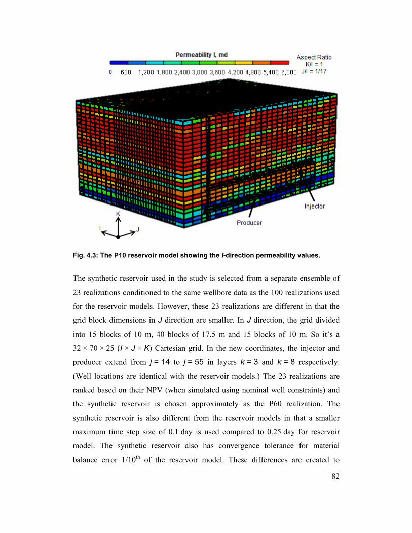
82

Fig. 4.3: The P10 reservoir model showing the I-direction permeability values.

The synthetic reservoir used in the study is selected from a separate ensemble of

23 realizations conditioned to the same wellbore data as the 100 realizations used

for the reservoir models. However, these 23 realizations are different in that the

grid block dimensions in J direction are smaller. In J direction, the grid divided

into 15 blocks of 10 m, 40 blocks of 17.5 m and 15 blocks of 10 m. So it’s a

32 × 70 × 25 (I × J × K) Cartesian grid. In the new coordinates, the injector and

producer extend from j = 14 to j = 55 in layers k = 3 and k = 8 respectively.

(Well locations are identical with the reservoir models.) The 23 realizations are

ranked based on their NPV (when simulated using nominal well constraints) and

the synthetic reservoir is chosen approximately as the P60 realization. The

synthetic reservoir is also different from the reservoir models in that a smaller

maximum time step size of 0.1 day is used compared to 0.25 day for reservoir

model. The synthetic reservoir also has convergence tolerance for material

balance error 1/10th

of the reservoir model. These differences are created to

83

replicate the differences between reservoir model predictions and real field

performance in reality, and to be able to judge the performance of MPC in

mitigating the uncertainty in reservoir models.

4.2. Well Configuration and Modeling

Long horizontal wells used in SAGD lead to non-uniform temperature profile and

steam flow along the wellbore because of the combined effects of reservoir

heterogeneity, frictional pressure drop and heat losses by conduction. The

accuracy with which these effects and the dynamic nature of SAGD are captured

by simulation models depends on the use of accurate well models. We model the

wells in our simulation study as Flexible Wellbores in STARS, which is an

advanced well modeling capability that discretizes the wellbore and solves the

wellbore equations simultaneously with the reservoir equations. This feature in

STARS allows modeling of up to three tubing strings inside an annulus. Packers

and ICDs/OCDs can also be included.

Further, as noted before, the wells in the simulation study have a dual tubing

string configuration. The dual tubing string in injector enables control of steam

injection into the heel and toe ends of the well, and the dual tubing string in

producer enables a differential steam trap control at the two ends of the well.

Also, the well containing blocks are refined into hybrid grid blocks. Each of these

blocks has 3 radial and 4 angular divisions to accurately model fluid flow around

the wellbore. The innermost radial division contains the well; the innermost block

doesn’t have any angular divisions.

The well dimensions that we use are summarized in Table 4.2. Other properties

related the wells including heat capacity and thermal conductivity of the wells,

relative roughness for pressure drop calculations and the maximum Nusselt

number allowed for heat transfer calculation are set to their defaults in STARS.

84

Table 4.2: Well dimensions used in our simulation study.

Parameter Value

Horizontal Well Length 720 m

Liner Location j = 4 to j = 25 in Reservoir Models

j = 14 to j = 55 in Synthetic Reservoir

Liner Perforations j = 6 to j = 25 in Reservoir Models


Short Tubing String Location j = 4 to j = 5 in Reservoir Models


Long Tubing String Location j = 4 to j = 25 in Reservoir Models


Packer Location j = 5 in Reservoir Models

j = 15 in Synthetic Reservoir

Liner ID/OD 0.219 m/0.241 m

Cement Thickness 0 m

Tubing ID/OD 0.076 m/0.089 m

4.3. Model-Based Optimization of Well Rates

For the P10 and P80 reservoir models, we use CMOST®

, version 2012.10

(CMOST 2012), for optimizing the well rates in SAGD production phase.

CMOST’s DECE (Designed Exploration and Controlled Exploration)

optimization method is used (Yang et al. 2009). DECE combines experimental

design technique with an evolutionary algorithm to find the optimum parameter

values from the given candidate values.

Complete simulation period consists of 4 months of circulation phase, from

January to April 2013, and 6 years and 8 months of SAGD production phase,

85

from May 2013 to December 2019. The first 8 months of the production phase are

left out of optimization because of the relatively long simulation run times for this

period. The results for RTO using MPC that we report in this thesis also only

concern the remaining 6 years of production from 2014 to 2019. In the two

reservoir models, for the production phase, the short and long tubing strings in the

injector have the maximum steam injection rate in Cold Water Equivalent (CWE)

as the primary well constraint. Further, a secondary well constraint of maximum

injection pressure of 9000 kPa is used. (Note that the simulator tries to operate a

well so that its primary constraint is satisfied; if it can’t be satisfied because a

secondary constraint is being violated, then that secondary constraint is used for

operating the well.) The short and long tubing strings in the producer have the

maximum steam production rate as their primary constraint. In STARS, a

maximum steam production rate constraint specifies the total volume of water

phase that is produced as vapor under downhole conditions, expressed in CWE.

Secondary constraints used for the producer strings are a minimum BHP of 102

kPa and maximum production rate of 300 m3/d of STL.

In CMOST, we specify the primary constraint values for injector and producer as

the optimization parameters. The different optimization intervals are January–

June 2014 (2014-1), July–December of 2014 (2014-2), January–June 2015 (2015-

1), July–December 2015 (2015-2), January–June 2016 (2016-1), July–December

(2016-2), 2017, 2018 and 2019. Within each of these optimization intervals, the

values of optimization parameters remain constant for optimization. (Note that for

the first 8 months of SAGD production, the primary well constraints are fixed at

90 m3/d and 70 m

3/d steam injection rates in CWE for short and long tubing

strings respectively in the injector and 1 m3/d and 7 m

3/d maximum steam

production rates in the short and long tubing strings respectively in the producer.

The same constraints are also used for the wells in synthetic reservoir for this

period.) The candidate values (these are the values that CMOST will try) for

optimization parameters in each optimization interval are chosen based on the

86

pressures observed during SAGD production in test simulations and the general

trend of optimized rates found in the works of Gates and Chakrabarty (2006) and

Yang et al. (2011). Gates and Chakrabarty (2006), who used a heterogeneous 2D

model, used a genetic algorithm to optimize steam injection pressures in 13 time

intervals over a total SAGD simulation period of 6 years. (At the producer, the

steam trap constraint in STARS was used, and a steam trap subcool of 5°C was

implemented). In the optimized profile that they found, shown in Fig. 4.4,

injection pressure was high at the beginning of SAGD production phase, when all

the heat is going to the bitumen formation. The pressure peaked again just before

the steam chamber hit the overburden, which according to the authors of the work

can be thought of as “overcoming thermal inertia”. After hitting the overburden,

as the steam chamber laterally expanded, the pressure continuously decreased to

reduce heat losses to the overburden. Yang et al. (2011), who used a 2D model

with three well pairs, also found a similar injection profile from optimization.

They used a maximum pressure constraint for the injector and maximum steam

rate constraint for the producer, both of which were optimized.

87

Fig. 4.4: Optimum steam injection pressures in 13 time intervals for the 2D model

used in Gates and Chakrabarty (2006).

The candidate values that we use in this work for the optimization parameters in

each optimization interval in the case of P10 reservoir model are shown in Table

4.3. Table 4.4 shows the values for P80 reservoir model. The optimized values

found by CMOST are underlined in the two tables. The P10 model was the first to

be optimized. The optimum values found in the P10 case helped us in choosing a

more narrow range of candidate values for the optimization parameters in P80

case. The range of candidate values for an optimization parameter was

approximately centered around the optimum value found in the P10 case. As a

result, as can be seen in the figures in the next section, the results of CMOST

optimization in the P80 case are better than the P10 case.

88


values found by CMOST are underlined.

Optimization

Parameters

Optimization Intervals

2014-1 2014-2 2015-1 2015-2 2016-1 2016-2 2017 2018 2019

Heel Injection

Rate (m3/d)

70 80

90 100

110 120

70 80

90 100

110 120

70 80

90 100

110 120

140

70 80

90 100

110 120

140

70 80

90 100

120 140

150 160

70 80

90 100

120 140

150 160

50 60

70 80

90 100

120

50 60

70 80

90 100

40 50

60 70

80 90

100

Toe Injection

Rate (m3/d)

70 80

90 100

110 120

70 80

90 100

110 120

70 80

90 100

110 120

140

70 80

90 100

110 120

140

70 80

90 100

120 140

150 160

70 80

90 100

120 140

150 160

50 60

70 80

90 100

120

50 60

70 80

90 100

40 50

60 70

80 90

100

Heel Maximum

Steam Rate

Constraint

Value (m3/d)

1 1.5 2

2.5 3 4

5 7

1 1.5 2

2.5 3 4

5 7

1 1.5 2

2.5 3 4

5 7

1 1.5 2

2.5 3 4

5 7

1 1.5 2

2.5 3 4

5 7

1 1.5 2

2.5 3 4

5 7

1 1.5 2

2.5 3 4

5 7

1 1.5 2

2.5 3 4

5 7

1 1.5 2

2.5 3 4

5 7

Toe Maximum

Steam Rate

Constraint

Value (m3/d)

2.5 3 4

5 6 6.5

7 7.5 8

2.5 3 4

5 6 6.5

7 7.5 8

2.5 3 4

5 6 6.5

7 7.5 8

2.5 3 4

5 6 6.5

7 7.5 8

2.5 3 4

5 6 6.5

7 7.5 8

2.5 3 4

5 6 6.5

7 7.5 8

2.5 3 4

5 6 6.5

7 7.5 8

2.5 3 4

5 6 6.5

7 7.5

8.0

2.5 3 4

5 6 6.5

7 7.5 8

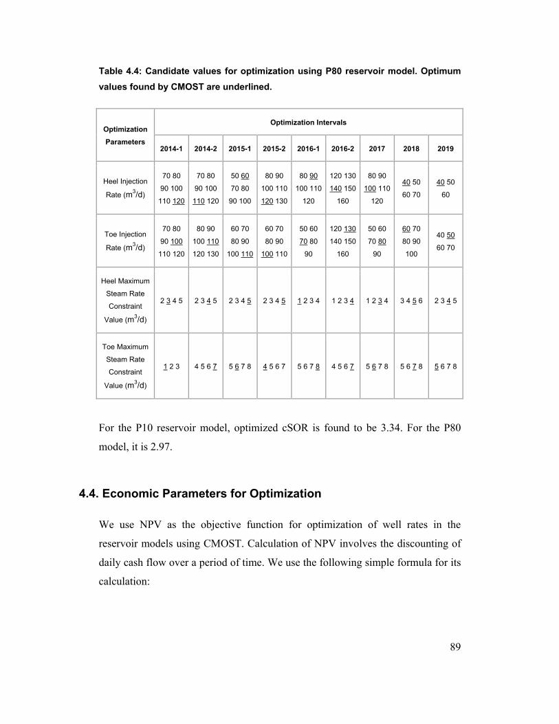
89


values found by CMOST are underlined.

Optimization

Parameters

Optimization Intervals

2014-1 2014-2 2015-1 2015-2 2016-1 2016-2 2017 2018 2019

Heel Injection

Rate (m3/d)

70 80

90 100

110 120

70 80

90 100

110 120

50 60

70 80

90 100

80 90

100 110

120 130

80 90

100 110

120

120 130

140 150

160

80 90

100 110

120

40 50

60 70

40 50

60

Toe Injection

Rate (m3/d)

70 80

90 100

110 120

80 90

100 110

120 130

60 70

80 90

100 110

60 70

80 90

100 110

50 60

70 80

90

120 130

140 150

160

50 60

70 80

90

60 70

80 90

100

40 50

60 70

Heel Maximum

Steam Rate

Constraint

Value (m3/d)

2 3 4 5 2 3 4 5 2 3 4 5 2 3 4 5 1 2 3 4 1 2 3 4 1 2 3 4 3 4 5 6 2 3 4 5

Toe Maximum

Steam Rate

Constraint

Value (m3/d)

1 2 3 4 5 6 7 5 6 7 8 4 5 6 7 5 6 7 8 4 5 6 7 5 6 7 8 5 6 7 8 5 6 7 8

For the P10 reservoir model, optimized cSOR is found to be 3.34. For the P80

model, it is 2.97.

4.4. Economic Parameters for Optimization

We use NPV as the objective function for optimization of well rates in the

reservoir models using CMOST. Calculation of NPV involves the discounting of

daily cash flow over a period of time. We use the following simple formula for its

calculation:

90

N

o o w w

k ref

t Q r - Q r =

t - tDt

1

NPV(1+ )

. ....................................(4.1)

Here, t1 is the starting time for calculating cash flow in days, tN is the ending time

in days. Qo is the oil produced in a day, ro is the oil price, Qw is the steam injected

in CWE in a day, rw is the steam generation cost and D is the discount factor. tk

goes from t1 to t2. tref is the time to which all cash flow is discounted . For the

reservoir models, NPV is calculated from 01-01-2014 to 01-01-2020. Cash flow is

discounted to the start of 2014. Oil price used is 8 $/bbl and steam generation cost

is fixed at 50 $/bbl CWE. A discount factor of 0.1 a year is used.

Fig. 4.5 shows the CMOST objective function evaluations (the jobs) for the P10

reservoir model. Fig. 4.6 shows the objective function evaluations for the P80

reservoir model. Each job is a simulation of the reservoir model for the

optimization period (6 years from 2014 to 2019) using a given set of optimization

parameter values. Simulation of the 6 years of production roughly took between 1

hour and 1.5 hours (considering the fact that in the two CMOST runs, we ran two

jobs concurrently most of the time). Further, a job restarts from a previous job,

instead of simulating the whole 6 years, if an initial set of optimization parameters

values being used for the job is identical to that of the previous job, which helps

cut the simulation time. Certain jobs in the CMOST runs, which took an

unusually large time to simulate, were terminated when the run time reached a set

maximum amount (as many as 8 hours). Objective function isn’t evaluated for

these jobs. In the P10 case, the CMOST run consisted of a total of 1452 jobs and

lasted a little more than 3.5 months with an Intel®

CoreTM

i7-2600 3.40 GHz

processor and 12 GB RAM, whereas in the P80 case, 1476 jobs needed around 3

months.

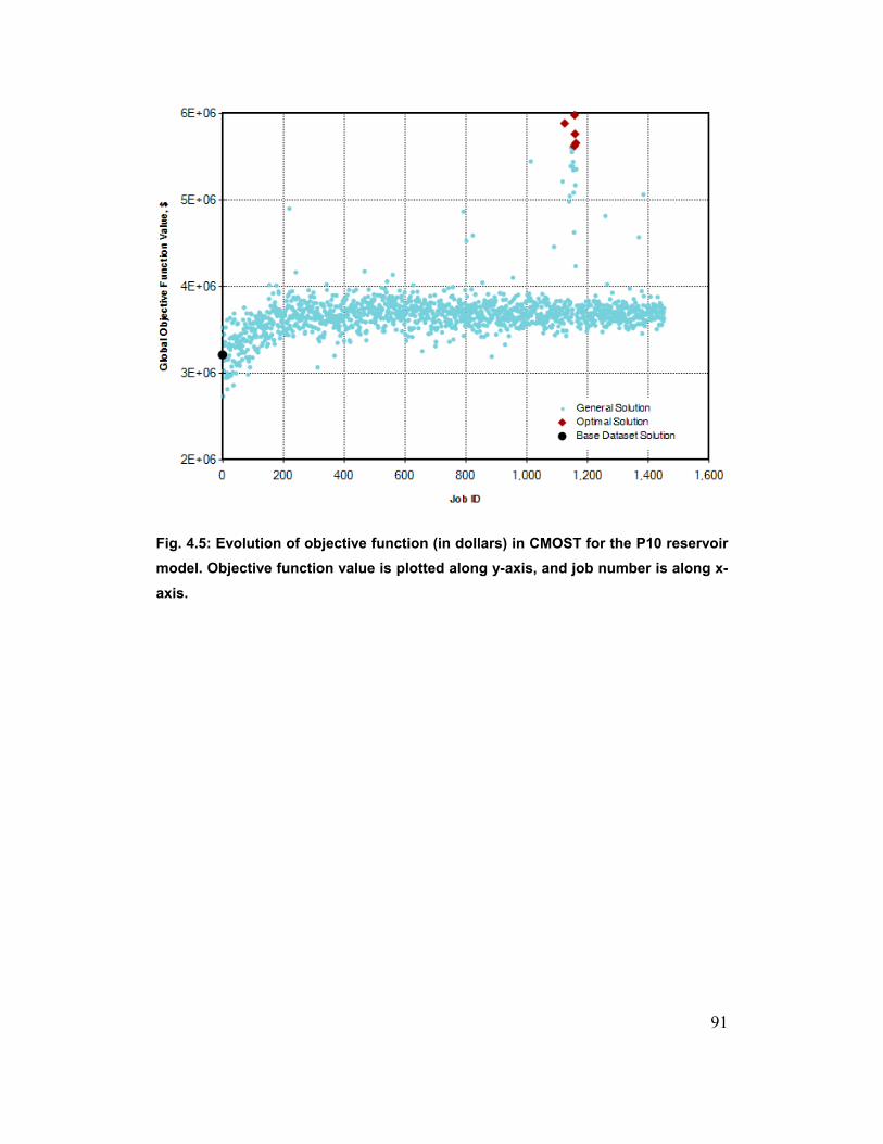
91

Fig. 4.5: Evolution of objective function (in dollars) in CMOST for the P10 reservoir

model. Objective function value is plotted along y-axis, and job number is along x-

axis.

92

Fig. 4.6: Evolution of objective function (in dollars) in CMOST for the P80 reservoir

model. Objective function value is plotted along y-axis, and job number is along x-

axis.

4.5. Interwell Subcool Control

(In the remainder of the thesis, we refer to the short-tubing string rates in a dual

tubing string well as heel rates and the long-tubing string rates as toe rates for the

sake of brevity.)

A workflow created in MATLAB integrates STARS, Results Report®, version

2013.10 (Results Report 2013), the System Identification Toolbox and the Model

Predictive Control Toolbox to control the subcool along SAGD well pair in

synthetic reservoir. The inputs that are manipulated for controlling the process are

the heel/toe steam injection and oil production rates. Hence, these (the heel and

toe rates) are used as the primary well constraints in the synthetic reservoir

93

created in STARS (the secondary well constraints remain the same as the

reservoir models). To control subcool along the well pair, the primary well

constraint values in synthetic reservoir are changed every sampling interval to

reflect the rates calculated by the MPC controller. (We note that instead of the oil

production rate, total production rate would have been a better choice for input

because in practice, choke settings are varied to control the production rate.)

The controlled variables are the heel subcool and the toe subcool. For control

purpose, the heel subcool in synthetic reservoir is defined as the average of

temperatures in the innermost hybrid refined blocks in the injector well blocks

from j = 16 to j = 35 (i.e., the heel half of the well pair after the packer) less the

average of temperatures in the corresponding innermost hybrid refined blocks in

the producer well blocks. Toe subcool is defined similarly based on the well

blocks from j = 36 to j = 55 (i.e., the toe half of the well pair after the packer).

The heel subcool and toe subcool set points for MPC are calculated from the

reservoir models for the same well intervals (j = 6 to j = 15 for heel subcool and

j = 16 to j = 25 for toe subcool in the two reservoir models).

Fig. 4.7 shows how the MATLAB workflow used for identification and control in

our simulation study works.

94

Fig. 4.7: A schematic representation of the MATLAB workflow used for identifying

linear models and controlling the SAGD wells in synthetic reservoir.

Because SAGD is a time-varying process, multiple identification periods are

required for the system identification model to correctly represent the input-output

relationships, which is necessary for a stable control performance. In our

simulation study, we demarcate two identification plus control periods—the first

such that it is roughly till the point in time when the steam chamber hits the

95

overburden and the second, after this event—each consisting of a control period

preceded by an identification period based on which an ARX model is identified,

which is then used for MPC of subcool along the well pair in reservoir. We chose

the ARX model because there is no disturbance in our synthetic process—SAGD

in the synthetic reservoir. The signal-to-noise ratio is zero and this allows us to

use the simple ARX model rather than a more complex linear dynamic model

structures like the BJ model, in which the disturbance dynamics are modeled fully

independently of the process dynamics.

In both the P10 and P80 reservoir model cases, the first identification plus control

period is the first three years from 2014 to 2016, and the second is the latter three

years from 2017 to 2019. We choose the second identification plus control period

to start from 2017 based on the optimum rate profiles for the reservoir models. As

can be noted from Table 4.3 and Table 4.4 as well as the figures in Chap. 5, the

optimum injection rates peak in the second half of 2016, which signifies that the

steam chamber hits the overburden in this period. Starting the second

identification plus control period after the steam chamber hits the overburden

ensures that the rates are more similar for the period. That way, an ARX model

identified in the beginning of the period will have a better predictive ability over

the whole period.

The only difference between the P10 and P80 reservoir model cases is that the

actual identification period, which prepares the data for identification, starts from

January 2014 in the former whereas in the latter, it starts from July 2014, followed

by a control period till the end of 2016. The first 6 months of 2014 are left out of

identification and control in the P80 case as the optimum toe oil rate obtained

from the reservoir model (corresponding to the optimum maximum steam rate

constraint value obtained from CMOST) for this period is zero. (Note that this

will happen if the long tubing string in the reservoir model is shut in by the

simulator because the secondary constraint value can’t be satisfied.) Table 4.5

96

contains the starting and ending points for the identification and control periods,

with the point of time in simulation mentioned in parentheses.

Table 4.5: Identification and control periods. Any differences in the P80 case are

noted.

Periods Start End

First Identification Period

01/01/2014 (365 days) for

P10.

01/08/2014 (577 days) for

P10.

01/07/2014 (546 days) for

P80.

01/02/2015 (761 days) for

P80

First Control Period

01/08/2014 (577 days) for

P10. 01/01/2016 (1461 days) for

P10. 01/02/2015 (761 days) for

P80.

Second Identification

Period 01/01/2017 (1461 days) 01/08/2017 (1673 days)

Second Control Period 01/08/2017 (1673 days) 01/01/2020 (2556 days)

Prior to running the MATLAB workflow represented in Fig. 4.7 for our

simulation study, we simulated the synthetic reservoir a number of times to

determine how to best identify an ARX model. The input-output data (injection

rates, oil rates, heel subcool and toe subcool) recorded from these simulations was

divided into two identification plus control periods, just as planned for the

simulation study, and for each of the periods, an initial part of the data was used

to estimate an ARX model, and the rest was used to validate the identified model.

A number of simulations were required as we found it very difficult to identify a

model that performed reasonably well in validation—we will come back to the

97

issues in identification and control and identify the causes in Section 6.1. Hence,

we used a trial-and-error approach to design the identification phase.

Based on the trial simulations of synthetic reservoir, we decided to keep the

identification periods 7 months long in our simulation study, which is also evident

from Table 4.5. The first 3 months of the 7 months, injection rates and oil

production rates are held constant at the corresponding average values of

optimum rates obtained from the reservoir model for the 7 months. The remaining

4 months, RBS signals with zero mean are superimposed on the average rates; an

ARX model is identified based on the input-output data from these 4 months only.

(Precisely the RBS signals start after the first 2 days of this 4-month period so that

the identification data has a short steady state-like part in the beginning.) Note

that in the reservoir models, the well constraints values that were varied for

optimizing the NPV were the maximum steam injection rates and the maximum

steam production rates. However, in the synthetic reservoir, wells are operated by

specifying the steam injection rates and oil production rates (these values are

manipulated by the MPC controller for optimizing the production). Hence, the

RBS signals for identification in synthetic reservoir are also for the steam

injection and oil production rates. In the identification periods, the optimum oil

rates (corresponding to the constant optimum steam injection and steam

production rates during the period) and hence the subcool exhibit a transient

behavior for the first 3 months, when they are seen to fluctuate a lot. We noted

during the trial simulations that keeping the oil production rates constant in these

3 months to prepare the data for identification leads to acceptable validation

results for the identified model. This explains our choice of an initial 3 months of

constant rates in the identification periods.

For identification of a linear model of a nonlinear process about an operating

point, the choice of amplitude of the identification signal is a trade-off between a

good signal-to-noise ratio and a close-to-linear process response (see Section 3.6).

Large changes in the signal increases the error in identified model because of the

98

system nonlinearity. On the other hand, using a small amplitude leads to a low

signal-to-noise ratio in the measurements. However, as noted before, signal-to-

noise ratio isn’t an issue in our simulation study. We choose amplitudes which are

just large enough to cause a clear change in the subcool. (We ran four small

simulations using the P10 reservoir model for the first 4 or 7 months of 2014, in

each of which a step change in one of the four primary constraint values

(maximum steam injection rate and maximum steam production rate) was

introduced after the first 2 months to observe the effect on the heel subcool and

toe subcool compared to a base case in which the constraint values are constant

throughout.) For identifying the ARX models in our simulation study, for the RBS

signals for injection rates and oil production rates, we choose amplitudes of 5

m3/d (so there are step changes of 10 m

3/d) and 1 m

3/d respectively for the first

identification period in 2014 and 15 m3/d and 1 m

3/d respectively for the second

identification period in 2017. We choose a much higher amplitude for the

injection rate RBS signals in second identification period as the response of

subcool to changes in injection rates is much smaller in second identification plus

control period. This is further explained below; it is also evident in the plots of

inputs and outputs with MPC and without MPC given in Chap. 5.

For an acceptable model performance, the linear models are identified separately

for the two outputs, and the two MISO models are combined to form a single

MIMO model for use in the MPC controller. For the first identification period, the

modified form of the ARX model structure that includes noise integration, the

ARIX model (given by Eq. 3.30 in a SISO case), is used for identification of a

model for heel subcool. And for the second identification period, the ARIX model

is used for both heel subcool and toe subcool. The need for using the ARIX model

was identified in the trial simulations that we did using the synthetic reservoir.

While looking into the validation results for the heel subcool model identified in

the first identification period, we observed that the heel subcool data shows a

drifting character. This prompted us to try the ARIX model, which vastly

99

improved the model quality to give a validation performance that was marginally

reasonable such that we could use it in the MPC controller in our simulation

study. This is shown in the figures that follow. We surmise that the improvement

in performance is because the drifting nature of the output gets modeled as noise,

which otherwise introduces big errors into the identified models.

In the MATLAB workflow that we use in this work, the function arx is used to

build the MISO models, specifying the property values appropriately for

integrating noise, if required. Further, the function idpoly is used to combine the

MISO models into a single MIMO model, specifying each element of the D array

as 1 − q−1 to integrate noise, if required, for the corresponding output (see Eq.

3.30 and Section 3.4).

The plots in Figs. 4.8 and 4.9 (which are for first, 365–1461 days, and second,

1461–2556 days, identification plus control periods respectively) represented by a

solid black line show heel subcool and toe subcool data recorded during two

different trial simulations of synthetic reservoir. In these simulations, the optimum

well settings from P10 reservoir model were used. During the identification

periods outlined in Table 4.5 for the P10 case, the injection and oil production

rates were initially held constant and then RBS are superimposed, as described

previously. For the rest of the simulation, rates corresponding to the optimum well

settings from the P10 reservoir model were directly used. For system

identification, we chose a sampling interval of 0.25 day (see below); hence, for

simulating the synthetic reservoir, the primary constraint values were specified at

intervals of 0.25 day so that the input-output data for identification could be

recorded at these intervals from the simulation. Further, in each of the two

identification plus control periods, models—a model each for the heel subcool

and toe subcool—are identified using the identification period input-output data

recorded from the synthetic reservoir, and simulated to observe the match with the

subcool data for the whole identification plus control period to validate the

models. Plots represented by a dashed line in Figs. 4.8 and 4.9 show the

100

simulation results for identified models. The figures were obtained from the

graphical user interface (GUI) of System Identification Toolbox. Before an

identified model is simulated (or predicted) in the GUI, the initial conditions are

estimated to minimize the prediction error. Note that no noise is added to the

model output for simulation; i.e., the stochastic component in the identified model

is disregarded (see Section 3.5).

Fig. 4.8: Simulation performance of models identified for heel subcool (top) and toe

subcool, represented by a dashed line, against data recorded from a trial

simulation of synthetic reservoir, for the first identification plus control period.

101

Fig. 4.9: Simulation performance of models identified for heel subcool (top) and toe

subcool, represented by a dashed line, against data recorded from a trial

simulation of synthetic reservoir, for the second identification plus control period.

Corresponding to the subcool data in Fig. 4.8, Figs. 4.10 and 4.11 show the steam

injection and oil production rates respectively that were used in the synthetic

reservoir in first identification plus control period, 365–1461 days. It can be noted

in these figures that there is an initial identification period of 7 months, 365–577

days, in which the rates are first held constant and then 4-month long RBS signals

are superimposed, as noted before. The RBS signals have amplitudes of 5 m3/d

and 1 m3/d for the steam injection rates and oil production rates respectively.

Corresponding to the subcool data in Fig. 4.9, we used amplitudes of 10 m3/d and

1 m3/d for the steam injection rates and oil production rates respectively. (Note

that for the toe oil rate in Fig. 4.11, an initial part of the RBS signal couldn’t be

102

used for operating the well as the secondary well constraint (a minimum BHP of

102 kPa) was violated. Nonetheless, the input-output data for the whole 4 months

was used for identifying the heel subcool and toe subcool models. We do the

same when we use the MATLAB workflow represented in Fig. 4.7 for our

simulation study in the P10 reservoir model case.)

Fig. 4.10: Heel (top) and toe injection rates used for the first identification plus

control period in the trial simulation of synthetic reservoir corresponding to Fig.

4.8.

103

Fig. 4.11: Heel (top) and toe oil rates used for the first identification plus control

period in the trial simulation of synthetic reservoir corresponding to Fig. 4.8.

Compared to Fig. 4.8, Fig. 4.12 shows that there is a drastic drop in the simulation

performance of identified heel subcool model if the ARX model is used instead of

the ARIX model in the first identification plus control period. Similarly, Fig. 4.13

shows the poor simulation performance, compared to Fig. 4.9, of the ARX model

for heel subcool in second identification plus control period.

104

Fig. 4.12: Simulation performance of ARX model for heel subcool, represented by a

dashed line, against data recorded from the trial simulation of synthetic reservoir

corresponding to Fig. 4.8, for the first identification plus control period.

Fig. 4.13: Simulation performance of ARX model for heel subcool, represented by a

dashed line, against data recorded from the trial simulation of synthetic reservoir

corresponding to Fig. 4.9, for the second identification plus control period.

In Figs. 4.8 and 4.9, to analyze the simulation performance of the identified

models we attached importance to whether the simulated subcool moved in the

same direction as the recorded subcool, especially at the beginning of the

optimization intervals that were outlined in Section 4.3, when step changes in the

recorded subcool data can be seen in these figures. This is necessary for MPC to

drive the inputs in right direction to control the subcool. (Note that in Figs. 4.8

and 4.9, the identified models match the initial 7 months of the subcool data well

105

as this is the same data that is used for identification.) The satisfactory

performance of the models in this respect gave us the confidence to use them for

MPC of subcool along the well pair in synthetic reservoir. E.g., in Fig. 4.8, the

identified heel subcool model for first identification plus control period correctly

follows the step changes in subcool. However, we also note that the long term

subcool trends within the optimization intervals are incorrect; further, the toe

subcool model in second identification plus control period in Fig. 4.9 doesn’t

respond correctly in the last year of the data (2019). Apart from looking at the

trends in simulated output, we paid attention to what the input-output

relationships were, whether positive or negative, in the identified models.

Particularly, we expected from the four small simulations of the P10 reservoir

model that we did, in which we used step changes in the primary constraints

values, that the heel injection rate-heel subcool relationship is positive and heel

oil rate-heel subcool relationship is negative. Table 4.6 shows the gain for each

input-output relationship in the identified models in Figs. 4.8 and 4.9. These gains

were noted from the GUI of System Identification Toolbox. We had used the

same GUI for identifying the models from data from the trial simulations of the

synthetic reservoir. A positive gain means a positive relationship between the

input and output, and, conversely, a negative value shows a negative relationship.

We note in Table 4.6 how the heel injection rate-heel subcool and toe injection

rate-toe subcool gains in first identification period are about five times higher than

in the second period. This explains why we choose a higher amplitude for the

RBS signals for injection rates in the second identification period (15 m3/d

compared to 5 m3/d in the first identification period) in the MATLAB workflow

that we use for our simulation study. We will further comment on the magnitudes

of observed gains in Section 6.1.

106

Table 4.6: Model gains in °C/m3/d for the heel subcool and toe subcool models

identified in first and second identification periods from the data recorded from

trial simulations of synthetic reservoir.

First Identification Period Second Identification Period

Heel Subcool Toe Subcool Heel Subcool Toe Subcool

Heel Injection

Rate +0.048 +0.111 +0.012 −0.055

Toe Injection

Rate −0.033 −0.025 +0.006 −0.004

Heel Oil Rate −0.444 +0.264 −0.221 −0.500

Toe Oil Rate +1.274 −0.464 −0.062 −0.680

Compared to the simulation performances in Figs. 4.8 and 4.9, the 20-step

prediction performance (see Section 3.5) for the identified heel subcool models in

first and second identification plus control intervals are shown in Figs. 4.14 and

4.15 respectively. Because we chose a sampling interval of 0.25 day for

identifying the models, a 20-step prediction horizon means the output is predicted

at t is made using past recorded input data, and past recorded output data up to t –

5 days. We note from the prediction performance figures that it is not easy to

discern the model quality because the 20-step prediction will simply tend to stay

close to the recorded output, even in cases when the identified models have large

errors in them. So, we relied on the simulation performances to judge the model

quality.

107


represented by a dashed line, against data recorded from the trial simulation of

synthetic reservoir corresponding to Fig. 4.8, for the first identification plus control

period.


represented by a dashed line, against data recorded from the trial simulation of

synthetic reservoir corresponding to Fig. 4.9, for the second identification plus

control period.

We noted in Section 3.6 that for using an identified model in a model-based

controller, the rule of thumb is to use a sampling interval, Ts, that is 0.1–0.2 times

the time constant of the process and a bandwidth of [0 pTs / πτ], expressed as a

fraction of Nyquist frequency. For the identified models in Figs. 4.8 and 4.9, we

roughly estimated the time constants and noted the approximate settling times

from the GUI of System Identification Toolbox. To do so, we looked at the step

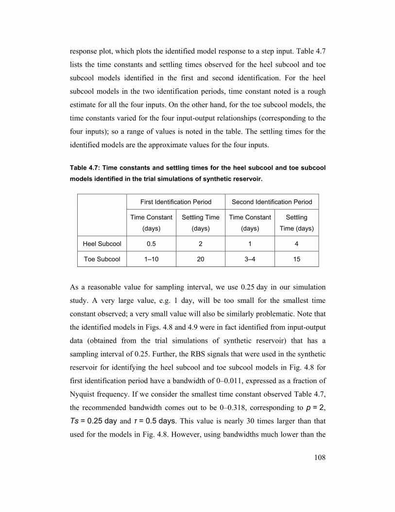
108

response plot, which plots the identified model response to a step input. Table 4.7

lists the time constants and settling times observed for the heel subcool and toe

subcool models identified in the first and second identification. For the heel

subcool models in the two identification periods, time constant noted is a rough

estimate for all the four inputs. On the other hand, for the toe subcool models, the

time constants varied for the four input-output relationships (corresponding to the

four inputs); so a range of values is noted in the table. The settling times for the

identified models are the approximate values for the four inputs.

Table 4.7: Time constants and settling times for the heel subcool and toe subcool

models identified in the trial simulations of synthetic reservoir.

First Identification Period Second Identification Period

Time Constant

(days)

Settling Time

(days)

Time Constant

(days)

Settling

Time (days)

Heel Subcool 0.5 2 1 4

Toe Subcool 1–10 20 3–4 15

As a reasonable value for sampling interval, we use 0.25 day in our simulation

study. A very large value, e.g. 1 day, will be too small for the smallest time

constant observed; a very small value will also be similarly problematic. Note that

the identified models in Figs. 4.8 and 4.9 were in fact identified from input-output

data (obtained from the trial simulations of synthetic reservoir) that has a

sampling interval of 0.25. Further, the RBS signals that were used in the synthetic

reservoir for identifying the heel subcool and toe subcool models in Fig. 4.8 for

first identification period have a bandwidth of 0–0.011, expressed as a fraction of

Nyquist frequency. If we consider the smallest time constant observed Table 4.7,

the recommended bandwidth comes out to be 0–0.318, corresponding to p = 2,

Ts = 0.25 day and τ = 0.5 days. This value is nearly 30 times larger than that

used for the models in Fig. 4.8. However, using bandwidths much lower than the

109

recommended bandwidth was a very significant conclusion that emerged from the

trial simulations of synthetic reservoir. E.g., Fig. 4.16 shows the simulation

performance for heel subcool and toe subcool models identified in first

identification period when a bandwidth of 0–0.064 is used, which is still nearly

five times lower than the recommended bandwidth; other things, including the

sampling interval, remain the same as the models in Fig. 4.8. The simulation

performance vastly degrades compared to Fig. 4.8. Hence, for identifying the heel

subcool and toe subcool models in our simulation study, we use a very low

bandwidth of 0–0.011.

110


toe subcool, represented by a dashed line, against data recorded from the trial


identification plus control period. To identify the models, RBS signals were used in

the synthetic reservoir that had a bandwidth that was one-fifth the recommended

amount. Other things, including the sampling interval, remain the same as the

models in Fig. 4.8.

In our simulation study, the low bandwidth for RBS signals leads to a need for a

much longer estimation period for the identified models compared to the rule of

thumb, which is to keep it at least five times the time constant of the process. As

noted before, we identify the models based on 4 months of input-output data. All

the identified models plotted above were identified using 4 months of data as

well. E.g., in Figs. 4.10 and 4.11, we can see in the initial part of the plots that the

low-bandwidth RBS signals only have a few (3–5) step changes. Hence, say, if we

111

use only 2 months, which would be half the length of the RBS signals in these

figures, the signal will excite very low frequencies in the process leading to a poor

identified model. As we will see in Chap. 5, this is indeed the case.

For MPC of subcool along the well pair in reservoir, because of the lesser than

expected performance of identified models (which we will discuss in Section 6.1),

we choose a relatively short prediction horizon of 5 days compared to the settling

times in Table 4.7; prediction over a longer horizon will anyways not be very

accurate as demonstrated in Fig. 4.17. The figure shows the prediction

performance of the identified toe subcool model shown in Fig. 4.8 for the first

identification plus control period. We can see that using 60-step (15-day)

prediction horizon, instead of a 20-step (5-day) horizon, deteriorates the

prediction performance to nearly the same as the simulation performance in Fig.

4.8. Further, for MPC in our simulation study, input and output weights for heel

and toe injection rates, oil rates and subcool (i.e., a total of four inputs and two

outputs) are 0.1, 0.1, 0.5, 0.5, 0.7 and 0.7 respectively. The input weights are

roughly chosen based on the observed gains of identified models from trial

simulations for different input-output relationships, as shown in Table 4.6.

Roughly speaking, let’s say, we consider a MISO process, the input changes

calculated by the MPC Controller will be proportional to the gains for the

different inputs if all the input weights are equal. Accordingly, in our case,

because we can see for the first identification period that the gains for oil rate on

an average much higher than for the injection rates, we keep oil rate weights five

times higher than the injection rate weights to keep the changes in oil rates as

calculated by the MPC controller smaller compared to changes in injection rates.

At the weights given above for the inputs, we try using higher weights, 1.0, for

the outputs, which leads to an unstable controller. We show a case of unstable

controller in Chap. 5. The failure of higher weights, again, arises from the weak

performance of the identified models.

112

Fig. 4.17: 20-step (top) and 60-step prediction performance of the model identified

for toe subcool, represented by a dashed line, against data recorded from the trial


identification plus control period.

Finally, we consider a few other identification details for the last part of this

discussion. All ARX/ARIX models in our simulation study have two poles and

one zero. Although not mentioned before, the identified models in the figures

above also have the same number of poles and zeros. The vital conclusions for

our simulation study that came out of the trial simulations of synthetic reservoir

were to use low-bandwidth RBS signals for the inputs in identification periods

and keep the identification periods long, with RBS signals superimposed on

constant rates. These conclusions improve the performance of identified models

just enough to be able to use them in the MPC controller in the simulation study.

113

Apart from these major conclusions, givdiscreteen the less-than-expected

performance of the identified models, when the model orders were varied for

identification of models from the input-output data from the trial simulations of

synthetic reservoir, no significant and consistent conclusions could be noted. So,

for the simulation study, we try to keep the model orders small without worrying

much as to its effect would be on performance and use the orders noted above.

Similarly, identifying the models by minimizing the one-step prediction error or

the simulation error (see Section 3.5) also didn’t seem significant. We choose the

latter for our simulation study. The identified models in the figures above also

minimized simulation error for estimation. Further, since the input-output data for

identification is in fact simulated data, from the synthetic reservoir, there is no

delay in it (i.e., outputs depend on the inputs instantaneously), as opposed to a

delay of one sampling interval that we had considered for the models in Chap. 3.

This arises from the way a simulator outputs information; the values output by the

simulator at any time represent the average amounts over the previous time step in

the simulation because the simulator equations are solved in discrete time.

However, the Model Predictive Control Toolbox, which we use in the MATLAB

workflow used in our simulation study, doesn’t accept models without a time

delay. Hence, in the MATLAB workflow a delay of one sampling interval is

artificially introduced in the input-output data prior to identifying linear models

by shifting the output data up a sampling interval. The models are then identified

with a delay of one sampling interval, which can subsequently be used in the

Model Predictive Control Toolbox. Also, the data for identification is not

detrended as the trends in recorded input-output data during the identification

period in the trial simulations are very different from the overall trends in the

identification plus control period.

We note that in the field, the engineer only has reservoir models at his disposal to

find suitable identification and control parameters. However, in our work, to be

able to understand and work around the several issues we had identifying

114

reasonable linear models, we took the liberty to use both the synthetic reservoir

and the P10 reservoir model to try different parameter values.

For the identification and control parameters that we use, the run time for the

MATLAB workflow used in our simulation study is of the order of a day with an

Intel®

CoreTM

i7-2600 3.40 GHz processor and 12 GB RAM. Most of this time is

taken for the simulation of synthetic reservoir.

115

5. Results

Using the P10 reservoir model to optimize injection and production rates and find

the subcool set points, MPC of subcool along the well pair in reservoir leads to an

18.23% improvement in NPV compared to a direct application of the optimized

rates. The contribution of the first identification plus control period (the first three

years of the SAGD production phase subject to RTO using MPC, 2014–2016 or

365–1461 days) to the net improvement is 8.60% and that of the second

identification plus control period (2017–2019 or 1461–2556 days) is 26.17%.

Table 5.1 lists the NPV, cumulative oil production and cSOR amounts with MPC

and without MPC for the whole 6 years, first identification plus control period and

second identification plus control period and shows the corresponding percentage

improvements with MPC as opposed to without MPC. Fig. 5.1 shows the heel and

toe injection rates with MPC and without MPC. Fig. 5.2 shows the heel and toe

oil rates with MPC and without MPC. Fig. 5.3 shows the MPC controller’s

tracking performance for the heel subcool and toe subcool. Note that without

MPC, the optimum injection and production rates are directly used for SAGD.

Hence, in Figs. 5.1 and 5.2, the plots without MPC, which are colored red, are

simply the optimum values obtained from the P10 reservoir model. In Fig. 5.3,

which shows the heel and toe subcool with MPC and without MPC, the black

dashed plots show subcool recorded from the P10 reservoir model when the

optimized rates found by CMOST are directly used. These form the set points for

the MPC controller. The red plots show the heel subcool and toe subcool recorded

from the synthetic reservoir when MPC is not used. The red plot deviates from the

black dashed plot because of the differences between the reservoir model and the

synthetic reservoir. The green plots are for heel subcool and toe subcool when

MPC is used for real-time production optimization of SAGD in the reservoir. It

can be seen that the toe subcool tracks better than the heel subcool.

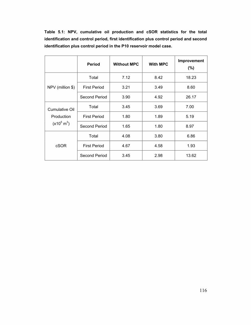
116


identification and control period, first identification plus control period and second

identification plus control period in the P10 reservoir model case.

Period Without MPC With MPC Improvement

(%)

NPV (million $)

Total 7.12 8.42 18.23

First Period 3.21 3.49 8.60

Second Period 3.90 4.92 26.17

Cumulative Oil

Production

(x105 m

3)

Total 3.45 3.69 7.00



cSOR

Total 4.08 3.80 6.86



117


MPC in the P10 reservoir model case.

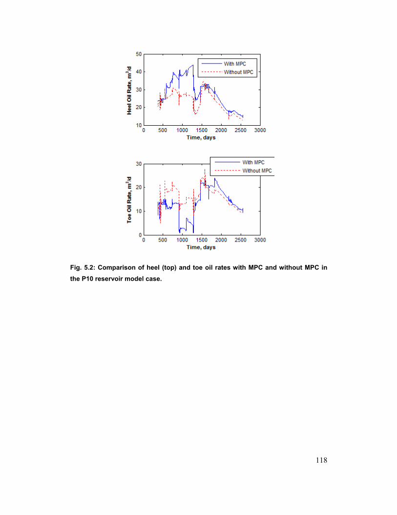
118

Fig. 5.2: Comparison of heel (top) and toe oil rates with MPC and without MPC in

the P10 reservoir model case.

119


the P10 reservoir model case. MPC tracks the set points.

In the P80 reservoir model case, using MPC to control the subcool along the well

pair in reservoir improves NPV by 8.81%, including the first 6 months of 2014

when no identification or control is done. The contribution of the first

identification plus control period (2014–2016 or 365–1461 days) to this

improvement is −0.59%, and that of the second identification plus control period

(2017–2019 or 1461–2556 days) is 21.02%. Table 5.2 lists the NPV, cumulative

oil production and cSOR amounts with MPC and without MPC for the total

period, first identification plus control period, and second identification plus

control period, and shows the corresponding percentage improvements with MPC

as opposed to without MPC. Fig. 5.4 shows the heel and toe injection rates with

MPC and without MPC. Fig. 5.5 shows the heel and toe oil rates with MPC and

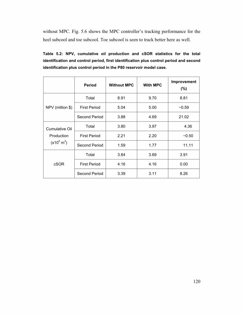
120

without MPC. Fig. 5.6 shows the MPC controller’s tracking performance for the

heel subcool and toe subcool. Toe subcool is seen to track better here as well.


identification and control period, first identification plus control period and second

identification plus control period in the P80 reservoir model case.

Period Without MPC With MPC Improvement

(%)

NPV (million $)

Total 8.91 9.70 8.81

First Period 5.04 5.00 −0.59


Cumulative Oil

Production

(x105 m

3)

Total 3.80 3.97 4.36

First Period 2.21 2.20 −0.50


cSOR

Total 3.84 3.69 3.91



121


MPC in the P80 reservoir model case.

122


the P80 reservoir model case.

123


the P80 reservoir model case. MPC tracks the set points.

We now explain a unique problem that the P80 reservoir model case posed, which

needed changes in the synthetic reservoir before the results presented above for

the P80 case could be obtained. As noted in Section 4.5, the optimum toe oil rate

obtained from the reservoir model for the first 6 months of 2014 is zero. Hence,

these first six months are excluded from any identification or control. Further, it

was seen that during the first and second identification plus control periods, when

we tried to use the optimum toe oil rate for simulating the synthetic reservoir, the

long tubing string was operating either at a fraction of that oil rate or was shut in a

lot of the simulation time, because of the violation of the secondary well

constraint (minimum BHP of 102 kPa) used for the long tubing string. In

retrospect, this is expected because the reservoir model is a P80 realization

124

whereas the synthetic reservoir is a P60 realization (see Section 4.1). Combined

with the high relative weights for oil rates used in the objective function for the

MPC controller in the MATLAB workflow that we use in in this work, this issue

with well constraints made MPC of subcool along the well pair in reservoir

unfeasible. Because the controller weights for oil rates are relatively high (0.1 for

heel and toe oil rates compared to 0.7 for the heel subcool and toe subcool), the

oil rates calculated by the controller to achieve the subcool set points remained

close to their optimum values; but when the toe oil rate calculated by the

controller for a sampling interval was used in the synthetic reservoir using the

MATLAB workflow, the long tubing string couldn’t be operated using that rate

because of the constraint issue. Ideally, we would have liked to lower the relative

weight for the oil rates to avoid the constraint issue, e.g., by using higher weights

for the outputs; however, as noted in Section 4.5, high outputs lead to controller

instability in our work due to the marginal performance of the identified linear

models in our work (also see below for an example of unstable controller action in

our work). To circumvent the issue with well constraints in the P80 reservoir

model case, we modify the producer well dimensions in the synthetic reservoir so

that the long tubing string can be operated at a higher oil rate than originally

possible. Liner ID/OD are reduced from their original values noted in Table 4.2,

0.219 m/0.241 m, to 0.139 m/0.161 m, and tubing ID/OD are reduced from

0.076 m/0.079 m to 0.036 m/0.049. (Note that this should change the NPV results

both without and with MPC.) However, despite this modification some of the

issue with the toe tubing string constraints remains as indicated by the rapidly

fluctuating toe oil rate in the second control period in Fig. 5.5—the toe oil rate

drops from the controller-calculated value when the secondary constraint gets

violated. Consequently, the heel subcool also shows large fluctuations with MPC

in the second control period, as seen in Fig. 5.6. This also results in minor

fluctuations in values calculated by the MPC controller for the injection rates and

the heel oil rate. (This happens because of the fact that the heel subcool and toe

subcool recorded from the synthetic reservoir at sampling instants feed back into

125

the controller based on which the states of the model that it uses are updated;

however, the controller is unable to “see” that the toe oil rate calculated by it in

the previous sampling interval is different from the rate at which the tubing string

actually operates in the presence of a constraint issue.)

For the P10 reservoir model case, Figs. 5.7 through 5.9 represent a scenario in

which the MPC controller is unstable. For these results, the linear models are

identified using only 2 months of input-output data as opposed to 4 months for the

results in Figs. 5.1 through 5.3. Hence, the total identification period length is 5

months, including the initial 3 months of constant rates prior to the RBS signals.

Combined with the low-bandwidth RBS signals used for identification (see

Section 4.5), this results in poor identified models, which consequently leads to

the controller instability.

126


MPC in the P10 reservoir model case when linear models are identified using only

2 months of input-output data.

127



months of input-output data.

128



months of input-output data. MPC tracks the set points.

In the MALAB workflow that we use for our simulation study, we use upper and

lower bounds on the inputs and input rates (i.e. the change in an input from one

sampling interval to another) for the objective function of the MPC controller (see

Eqs. 2.2). The upper bounds used for the injection rates, rate of change of

injection rates, oil rates and rate of change of oil rates are 180 m3/d, 10 m

3/d per

sampling interval, 100 m3/d and 2 m

3/d per sampling interval respectively. The

corresponding lower bounds are 20 m3/d, −10 m

3/d per sampling interval, 1 m

3/d

and −2 m3/d per sampling interval. In Figs. 5.7 and 5.8, the unstable controller

performance is highlighted by the fact that the injection rates are at their upper

bounds (180 m3/d) and the toe oil rate is at its lower bounds (1 m

3/d) for all or

129

most of the first control period. Correspondingly, this results in a very high heel

subcool and toe subcool in the first control period (577–1461 days), as shown in

Fig. 5.9. However, in the second control period (1673–2556 days) the controller

seems to be stable despite identification of linear models from only 2 months of

input-output data. Still, the controller is almost completely ineffective in tracking

heel subcool and toe subcool unlike what’s seen in Fig. 5.3; some of this can be

attributed to the fact that the controller is given worse conditions to begin with as

it has to act to bring down the high heel subcool and toe subcool at the end of the

first control period.

The net result of using only 2 months of input-output data for identification is that

NPV deteriorates by 47.46% when MPC is used to control the subcool along the

well pair in reservoir as opposed to without MPC. Out of this net decrease in

NPV, the first identification plus control period sees a decrease in NPV by

197.42%. In the second identification plus control period, NPV improves by

76.19%; however this is because of the fact that very little oil is produced in the

first period due to an unstable controller, rather than that the controller performs

very well.

130

6. Discussion, Conclusions and

Recommendation for Future Work

6.1. Discussion

In SAGD, unless steam bypasses the bitumen in place by directly travelling from

the injector to the producer, conduction is the main heat transfer mechanism

around the production liner. Because of the resulting sharp temperature gradients,

interwell subcool is a strong function of liquid level above the produce. In one of

his 2D simulations, Edmunds (2000) found that increasing drawdown from

injector to producer by 5 kPa increased subcool by around 30°C. Hence, a linear

model, having a high gain, should be easily identifiable between

injection/production rates, and interwell subcool at different points along the well

pair, based on historic production data, as long as the data contains sufficient

variation in the rates.

However, the models that we could identify in this work were quite the opposite

of this expectation. The gain values in general for the different input-output

relationships are of the order of 0.1 °C/m3/d, as noted in Table 4.6. We noted that

the models that could be identified from input-output data from the trial

simulations of synthetic reservoir have a marginally reasonable performance at

best when simulated to match the data. This is reflected in our simulation study as

a little higher than the chosen weights for heel subcool and toe subcool, relative to

the input weights, for the MPC controller leads to controller instability. Also,

identification is not as easy as expected. The rates need to be held constant for 3

months in identification periods before the use of RBS signals for identifying the

linear models, to be able to achieve a reasonably good model performance.

131

After an analysis of the results obtained in this work, with hindsight we conclude

that the lower than expected linear model performance is because of steam

breakthrough in the highly heterogeneous reservoir used.

In SAGD, with a dual tubing string well configuration, which is typically used in

practice, steam preferentially goes into some intervals due to heterogeneity and

the production temperature varies along the producer. Under these circumstances,

the optimum operating conditions for SAGD in a highly heterogeneous reservoir

involves a small amount of steam production along the producer; some steam

production also helps heat up the colder intervals (Edmunds and Gittins 1993).

Some steam production is acceptable as long as there is sufficient surface steam

treatment capacity available. This situation can be avoided by using intelligent

wells, which contain ICVs for a more uniform steam distribution in the injector

and differential steam trap control in different intervals in the producer.

So, soon after the start of production in SAGD using dual tubing string wells,

steam channels get established from injector to producer. It difficult to reverse the

steam breakthrough once it happens because of the high mobility ratio of steam,

and the steam channels are maintained throughout the life of the field (Stone et al.

2010). Even in 2D when heterogeneity is no longer a consideration, as analysis of

Edmunds (2000) showed, steam tends to stay in the producer after it breaks

through even after pressure differential between injector and producer is

somewhat reduced. This is a nonlinear effect in the SAGD process. (Such

nonlinearity is also observed when production is so low in an interval that the

injector gets submerged in the liquid pool. Once the liquid level rises above the

injector, the production temperature gets effectively decoupled from the liquid

pool level due to convective effects pointed out by Edmunds (2000).)

Steam breakthrough also occurs in the reservoir models used in this work, which

have a pair of dual tubing string wells. The temperature maps in Figs. 6.1a

through 6.1d show the steam chamber evolution with MPC and without MPC in

132

the J-K plane containing the wells in synthetic reservoir in the P10 reservoir

model case; steam is seen to break through even before the start of first

identification period, 01-01-2014 (365 days). We also note from Fig. 5.3 that the

optimum heel subcool obtained from optimization of well settings in the P10

reservoir model using CMOST is negative towards the end of simulation period.

The overall effect of the steam breakthrough is to impair the ability to control the

production stream subcool. This makes identification of a good linear model to

represent the process dynamics unfeasible due to the inherent nonlinearity arising

from the direct steam flow from the injector to the producer, and poses challenges

in the identification process. Stone et al. (2014), who used wells with a dual

tubing string configuration and PID controllers on the short and long injection

tubing strings to control interwell subcool, also find that the toe subcool failed to

reach its control target once steam broke through in the heel half of the producer.

Fig. 6.1a: Reservoir steam chamber shape on 01-01-2014 (365 days), before the

start of first identification period, when with MPC and without MPC cases are the

same.

133

Fig. 6.1b: Reservoir steam chamber shape without MPC (top) and with MPC on

01-01-2016 (1095 days) in the P10 reservoir model case. The temperatures of white

cells lie below the range of the temperature scale.

134

Fig. 6.1c: Reservoir steam chamber shape without MPC (top) and with MPC on



135

Fig. 6.1d: Reservoir steam chamber shape without MPC (top) and with MPC on



However, despite the issue with steam breakthrough, it is noted from Figs. 6.1a

through 6.1d that MPC is able to control the steam chamber growth and increase

the recovery within the limits of the process. In these figures, which have been

obtained from Results 3D®

, version 2013.10 (Results 3D 2013), the scale along

the well direction is smaller by a factor of 17 compared to the perpendicular

direction to show the entire grid dimension in the well direction. Near the middle

of the plane each grid block is 17.5 m in the well direction. Results 3D allows up

to a maximum of 25 intervals in the temperature scale. Accordingly, in each of

these figures a range for the temperature scale is selected so that the difference in

temperatures profiles between the wells with MPC and without MPC gets

highlighted. The white colored grid blocks couldn’t be accommodated within the

temperature scale and have temperatures below the range covered by the scale.

Fig. 6.1b shows that on 01-01-2016 (1095 days), with MPC the proportion of heat

136

being transferred to the reservoir in the heel half compared to the toe half is more

(this is evident from the fact that the coldest interwell regions in the heel half

warm up while not so much in the toe half) and the steam chamber is slightly

more uniform. At the same time, the total heat delivery is higher with MPC

(which agrees with Figs. 5.1 and 5.2, which show that with MPC, heel rates

increase and toe rates decrease in the first control period). On 01-01-2018 (1826

days), as shown in Fig. 6.1c, with MPC the near-producer temperatures are more

uniform (which would mean higher oil production rates and lower SOR), and the

total heat delivery is lower (which agrees with the lower heel and toe injection

rates in the second control period with MPC as seen in Figs. 5.1 and 5.2). On the

last date of simulation in our study, 01-01-2020 (2556 days), as shown in Fig.

6.1d, with MPC the steam chamber is more uniform and the total heat delivery is

lower. The net effect of these differences is an 18.23% improvement in NPV.

Corresponding to Figs. 6.1b through 6.1d, Figs. 6.2a through 6.2c show the

temperature profile in the blocks in the well plane in the layer k = 5, which lies in

between the wells, from j = 16 to j = 55 (i.e., the range of blocks that runs along

the whole length of the well after the packer). The distance on the x-axis in these

figures is measured from the center of the j = 16 block, and temperature is plotted

up to the center of j = 55 block. Within a block, the temperature remains constant.

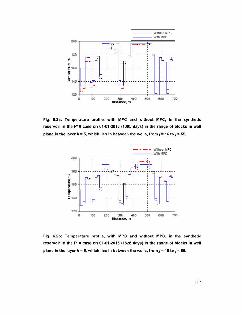
137

Fig. 6.2a: Temperature profile, with MPC and without MPC, in the synthetic

reservoir in the P10 case on 01-01-2016 (1095 days) in the range of blocks in well

plane in the layer k = 5, which lies in between the wells, from j = 16 to j = 55.

Fig. 6.2b: Temperature profile, with MPC and without MPC, in the synthetic



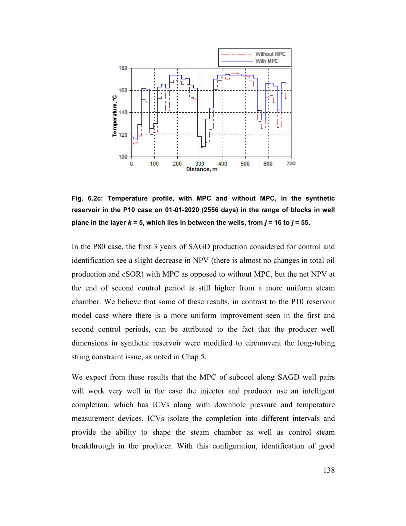
138

Fig. 6.2c: Temperature profile, with MPC and without MPC, in the synthetic



In the P80 case, the first 3 years of SAGD production considered for control and

identification see a slight decrease in NPV (there is almost no changes in total oil

production and cSOR) with MPC as opposed to without MPC, but the net NPV at

the end of second control period is still higher from a more uniform steam

chamber. We believe that some of these results, in contrast to the P10 reservoir

model case where there is a more uniform improvement seen in the first and

second control periods, can be attributed to the fact that the producer well

dimensions in synthetic reservoir were modified to circumvent the long-tubing

string constraint issue, as noted in Chap 5.

We expect from these results that the MPC of subcool along SAGD well pairs

will work very well in the case the injector and producer use an intelligent

completion, which has ICVs along with downhole pressure and temperature

measurement devices. ICVs isolate the completion into different intervals and

provide the ability to shape the steam chamber as well as control steam

breakthrough in the producer. With this configuration, identification of good

139

linear models will be much easier as opposed to the difficulties we face in our

simulation study, and real-time production optimization by means of the MPC

strategy will optimize the SAGD process. Gotawala and Gates (2012) have

already demonstrated the potential of ICVs to control steam flow with an

analytical 2D liquid pool model. They used a PID controller on the injection rates

to control the steam breakthrough and successfully revert to steam trap conditions,

and then maintain the subcool at a particular target. In the 3D model used by

Gotawala and Gates (2009), using PID control for the six ICVs along the injector,

a significant improvement in steam conformance was registered. The results

observed in these works highlight that a further extension of the MPC strategy

used in our work for RTO of the SAGD process to wells with ICVs is necessary

to obtain the desired results.

6.2. Conclusions

The following conclusions are drawn from our simulation study, with respect to

the hypothesis stated in the introduction to this thesis:

1. Despite the limitations of a dual tubing string well configuration in controlling

steam breakthrough in SAGD and the associated issue with identification of a

good linear model for MPC, the improvement in NPV with the application of

MPC to control the subcool along the well pair in reservoir in both the cases

considered in our numerical study helps us to conclude that MPC can be used

for real-time production optimization of SAGD. MPC considers all the

variables of the process while controlling it to improve the efficiency and

increase the oil recovery. At the same time, a unique capability of the MPC

strategy is that it allows handling of constraints on process variables. Hence,

MPC offers a more advanced control strategy compared to PID control, as used

in few other works for real-time optimization of SAGD.

140

2. In case of SAGD, it is possible to identify linear data driven models of the

process from the high frequency data from intelligent wells, which have

downhole pressure and temperature sensors, along with the use of surface

measurements. In our work, models were identified that related injection and

oil production rates to subcool along the SAGD well pair. To identify accurate

models, the inputs had to be held constant for a few months and then long RBS

signals with a very small bandwidth had to be used that lasted a further few

months. In practice, this won’t be feasible as the rates will move a lot.

However, this issue will be eliminated if intelligent wells with ICVs are used

to divide the production interval into isolated segments, in which steam

breakthrough can be individually controlled. In this case, because of a strong

relationship between the liquid pool level above the producer and the interwell

subcool, a process model could be identified simply based on the past

production data alone (which will normally have enough excitation in it for

good identification).

3. Additionally, a high accuracy of the identified linear models is not needed for

MPC. In the multilevel oilfield control framework that we consider in this

work, as discussed in the introduction to this thesis, the linear models used for

MPC only supplement the reservoir models, which are used to optimize the

injection/production plans. As such, they don’t need to capture the dynamics

accurately. In our work, because of the nonlinearity in the SAGD process due

to steam breakthrough very early into the production phase, it was not possible

to accurately represent the dynamics using linear models built from the input-

output data from the process using system identification. The best models that

could be identified based on the recorded input-output data from the trial

simulations of synthetic reservoir only have correct short-term subcool trends

when simulated to match the long-term data, as noted in Section 4.5. Despite

this, MPC is seen to track the subcool set points in both our cases. However, to

get the results, the output weights for MPC calculations had to be kept low in

order to avoid controller instability.

141

6.3. Recommendation for Future Work

Extending naturally from the discussion of results before, we recommend for

future a simulation study similar to the one done in this work, but with both the

injector and the producer having ICVs. E.g., the completion length used in this

work can be divided into four or five sections to control the steam chamber

independently in these sections. This will make identification of good linear

models for MPC easy and from a practical point of view, will be a much better

demonstration of the MPC strategy for real-time optimization of the steam

chamber growth and production.

Further, owing to the issues in system identification, our efforts in this work were

confined to obtaining workable linear models that we could use in the MPC

controller for controlling the subcool along the well pair in reservoir. We could do

so with ARX/ARIX models having two poles and one zero. Using wells with

ICVs, we could further investigate higher model orders to see if they improve the

validation performance significantly. Also, we used the ARX/ARIX models

because there were no disturbances in our synthetic reservoir. However, if actual

field data is used to estimate and validate linear models, different structures will

need to be tried to identify which noise assumption works the best. E.g., the BJ

model is suitable when the disturbance enters mostly at the output as

measurement noise. On a related matter, an active area of research in digital oil

fields is real-time cleansing of sensor data. Based on a statistical analysis, data

that is judged to be bad can be rejected and replaced. For further thoughts on how

real-time data from oil fields can be put to use, we refer to Rassenfoss (2013) and

Horne (2013).

142

Bibliography

Al-Mulhim, W., Mubarak, S.M., and Bonilla, J.C.G. 2013. What Is Next for

Intelligent Energy? Guest Editorial, Journal of Petroleum Technology 65

(10): 20–21.

Banerjee, S., Abdelfattah, T.A., and Nguyen, H.T. 2013. Benefits of Passive

Inflow Control Devices in a SAGD Completion. Paper SPE 165478

presented at the SPE Heavy Oil Conference-Canada, Calgary, Alberta,

Canada, 11–13 June. http://dx.doi.org/10.2118/165478-MS.

Bedry, M. and Shaw, J. 2012. Using a new Intelligent Well Technology

Completions Strategy to Increase Thermal EOR Recoveries - SAGD Field

Trial. Paper SPE 154760 presented at the SPE EOR Conference at Oil and

Gas West Asia, Muscat, Oman, 16–18 April. http://dx.doi.org/10.2118/

154760-MS.

Bemporad, A., Morari, M., and Ricker, N.L. 2012a. Model Predictive Control

Toolbox™ Reference R2012a. Natick, Massachusetts: The MathWorks,

Inc.

Bemporad, A., Morari, M., and Ricker, N.L. 2012b. Model Predictive Control

Toolbox™ User’s Guide R2012a. Natick, Massachusetts: The

MathWorks, Inc.

Huang, B. 2012. Process Identification. Lecture notes on input signals and

practical issues in process identification. Course CHE662, Fall 2012,

University of Alberta, Edmonton, Alberta.

Clark, H.P., Ascanio, F.A., Van Kruijsdijk, C.P.J.W. et al. 2010. Method to

Improve Thermal EOR Performance Using Intelligent Well Technology:

Orion SAGD Field Trial. Paper SPE 137133 presented at the Canadian

http://dx.doi.org/10.2118/%20154760-MS

http://dx.doi.org/10.2118/%20154760-MS

143

Unconventional Resources and International Petroleum Conference,

Calgary, Alberta, Canada, 19–21 October. http://dx.doi.org/10.2118/

137133-MS.

CMOST. 2012. CMOST Computer Assisted History Matching, Optimization and

Uncertainty Assessment Tool User’s Guide Version 2012. Calgary,

Canada: Computer Modelling Group Ltd.

ConocoPhillips. 2008. ERCB Annual Update: Surmont Project, June 4, 2008. In

Situ Performance Presentations, Data & Publications, Alberta Energy

Regulator, https://www.aer.ca/documents/oilsands/insitu-presentations/

ConocoPhillips_Surmont_Performance_Presentation.pdf (downloaded 25

August 2014).

Dilib, F.A. and Jackson, M.D. 2013. Closed-Loop Feedback Control for

Production Optimization of Intelligent Wells Under Uncertainty. SPE

Production & Operations 28 (4): 345–357 SPE-150096-PA.

http://dx.doi.org/10.2118/150096-PA.

Edmunds, N. 2000. Investigation of SAGD Steam Trap Control in Two and Three

Dimensions. Journal of Canadian Petroleum Technology 39 (1): 30–40.

PETSOC-00-01-02. http://dx.doi.org/ 10.2118/ 00-01-02.

Edmunds, N. and Chhina, H. 2001. Economic Optimum Operating Pressure for

SAGD Projects in Alberta. Distinguished Author Series, Journal of

Canadian Petroleum Technology 40 (12): 13–17. PETSOC-01-12-DAS.

http://dx.doi.org/10.2118/01-12-DAS.

Edmunds, N. and Gittins, S.D. 1993. Effective Application of Steam Assisted

Gravity Drainage of Bitumen to Long Horizontal Well Pairs. Journal of

Canadian Petroleum Technology 32 (6): 49–55. PETSOC-93-06-05.

http:// dx.doi.org/10.2118/93-06-05.

http://dx.doi.org/10.2118/%20137133-MS

http://dx.doi.org/10.2118/%20137133-MS

https://www.aer.ca/documents/oilsands/insitu-presentations/

http://dx.doi.org/10.2118/150096-PA

144

Foss, B.A. and Jensen, J.P. 2011. Performance Analysis for Closed-Loop

Reservoir Management. SPE Journal 16 (1): 183–190. SPE-138891-PA.

http://dx.doi.org/10.2118/138891-PA.

Gates, I.D. and Chakrabarty, N. 2006. Optimization of Steam Assisted Gravity

Drainage in McMurray Reservoir. SPE Journal of Canadian Petroleum

Technology 45 (9): 54–62. PETSOC-06-09-05. http://dx.doi.org/10.2118/

06-09-05.

Gates, I. D. and Leskiw, C. 2008. Impact of Steam Trap Control on Performance

of Steam-Assisted Gravity Drainage. Paper 2008-112 presented at the

Canadian International Petroleum Conference, 17–19 June, Calgary,

Alberta, Canada. http://dx.doi.org/10.2118/2008-112-EA.

Gonzalez, L.E., Ficocelli, P., and Bostick, T.X. 2012. Real Time Optimization of

SAGD Wells. Paper SPE 157923 presented at the SPE Heavy Oil

Conference Canada, Calgary, Alberta, Canada, 12–14 June. http://

dx.doi.org/10.2118/157923-MS.

Gotawala, D.R. and Gates, I.D. 2009. SAGD Subcool Control with Smart

Injection Wells. Paper SPE 122014 presented at the EUROPEC/EAGE

Conference and Exhibition, Amsterdam, The Netherlands, 8–11 June.

http://dx.doi.org/10.2118/122014-MS.

Gotawala, D.R. and Gates, I.D. 2012. A Basis for Automated Control of Steam

Trap Subcool in SAGD. SPE Journal 17 (3): 680–686. SPE-159170-PA.

http://dx.doi.org/10.2118/159170-PA.

Horne, R. 2013. Listening to the Reservoir – Interpreting Data from Permanent

Downhole Gauges PM. Distinguished Lecture Program Online webinar,

SPE Online Education Programs, 18 July 2013, http://

eo2.commpartners.com/users/spe/session.php?id=11058# (accessed 14

June 2014).

http://dx.doi.org/10.2118/138891PA

http://dx.doi.org/10.2118/%2006-09-05

http://dx.doi.org/10.2118/%2006-09-05

http://dx.doi.org/10.2118/159170-PA

145

Ito, Y. and Suzuki, S. 1999. Numerical Simulation of the SAGD Process In the

Hangingstone Oil Sands Reservoir. Journal of Canadian Petroleum


99-09-02.

Jacobs, T. 2014. Downhole Fiber-Optic Monitoring: An Evolving Technology.

Journal of Petroleum Technology 66 (8): 44–53.

Jansen, J.-D., Brouwer, R., and Douma, S.G. 2009. Closed Loop Reservoir

Management. Paper 119098 presented at the SPE Reservoir Simulation

Symposium, The Woodlands, Texas, 2–4 February. http://dx.doi.org/

10.2118/119098-MS.

Khan, M.A.B., Mehrotra, A.X., and Svrcek, W.Y. 1984. Viscosity Models For

Gas-Free Athabasca Bitumen. Journal of Canadian Petroleum


84-03-05.

Ljung, L. 1999. System Identification: Theory for the User, second edition. Upper

Saddle River, New Jersey: Prentice Hall Information and System Sciences

Series, Prentice Hall PTR.

Ljung, L. 2012a. System Identification Toolbox™ Reference R2012a. Natick,

Massachusetts: The MathWorks, Inc.

Ljung, L. 2012b. System Identification Toolbox™ User’s Guide R2012a. Natick,

Massachusetts: The MathWorks, Inc.

MATLAB®

, version V7.14 (release R2012a). Natick, Massachusetts: The

MathWorks, Inc.

Naus, M., Dolle, N., and Jansen, J.-D. 2006. Optimization of Commingled

Production Using Infinitely Variable Inflow Control Valves. SPE

http://dx.doi.org/10.2118/

http://dx.doi.org/%2010.2118/119098-MS

http://dx.doi.org/%2010.2118/119098-MS

http://dx.doi.org/10.2118/

146

Production & Operations 21 (2): 293–301. SPE-90959-PA. http://

dx.doi.org/10.2118/ 90959-PA.

Nelles, O. 2001. Nonlinear System Identification. Springer.

Nikolaou, M., Cullick, A.S., Saputelli, L.A. et al. 2006. A Consistent Approach

towards Reservoir Simulation at Different Time Scales. Paper SPE 99451

presented at the Intelligent Energy Conference and Exhibition,

Amsterdam, The Netherlands, 11–13 April. http://dx.doi.org/10.2118/

99451-MS.

Patel, K., Aske, E.M., and Fredriksen, M. 2014. Use of Model-Predictive Control

for Automating SAGD Well-Pair Operations: A Simulation Study. SPE

Production & Operations 29 (2): 105–113. SPE-165535-PA. http://

dx.doi.org/10.2118/165535-PA.

Perrons, R.K. and Jensen, J. 2014. The Unfinished Revolution: What is Missing

From the E&P Industry’s Move to “Big Data”. Guest Editorial, Journal of

Petroleum Technology 66 (5): 20–22.

Qin, S.J. and Badgewell, T.A. 2003. A Survey of Industrial Model Predictive

Control Technology. Control Engineering Practice 11 (7): 733–764.

http://dx.doi.org/10.1016/S0967-0661(02)00186-7.

Rassenfoss, S. 2013. Doing More With Data. Journal of Petroleum Technology

65 (5): 34–41.

Results 3D. 2013. Results 3D User’s Guide Version 2013. Calgary, Canada:

Computer Modelling Group Ltd.

Results Report. 2013. Results Report User’s Guide Version 2013. Calgary,

Canada: Computer Modelling Group Ltd.

http://dx.doi.org/10.2118/%2099451-MS

http://dx.doi.org/10.2118/%2099451-MS

147

Saputelli, L., Nikolaou, M., and Economides, M.J 2005. Self-Learning Reservoir

Management. SPE Reservoir Engineering and Evaluation 8 (6): 534–547.

SPE-84064-PA. http://dx.doi.org/10.2118/84064-PA.

Saputelli, L.A., Mochizuki, S., Hutchins, L. et al. 2003. Promoting Real-Time

Optimization of Hydrocarbon Producing Systems. Paper SPE 83978

presented at Offshore Europe, Aberdeen, UK, 2–5 September. http://

dx.doi.org/10.2118/83978-MS.

Seborg, D.E., Edgar, T.F., and Mellichamp, D.A. 2004. Process Dynamics and

Control, second edition. Hoboken, New Jersey: John Wiley & Sons, Inc.

Söderström, T. and Stoica, P. 2001. System Identification, 2001 edition. Hemel

Hempstead, Hertfordshire: Prentice Hall international series in systems

and control Engineering, Prentice Hall international (UK) Ltd.

STARS. 2013. STARS Advanced Processes & Thermal Reservoir Simulator

User’s Guide Version 2013. Calgary, Canada: Computer Modelling Group

Ltd.

Stone, T.W., Brown, G., Guyaguler, B. et al. 2014. Practical Control of SAGD

Wells With Dual-Tubing Strings. Journal of Canadian Petroleum

Technology 53 (1): 32–47. SPE-149352-PA. http://dx.doi.org/10.2118/

149352-PA.

Stone, T.W., Yardumian, H.E., Bailey, W.J. et al. 2010. Dynamic SAGD Well

Flow Control Simulation. Paper SPE 138054 presented at the Canadian

Unconventional Resources and International Petroleum Conference,

Calgary, Alberta, Canada, 19–21 October. http://dx.doi.org/10.2118/

138054-MS.

Suncor. 2013. Suncor Firebag 2013 ERCB Performance Presentation,

Commercial Scheme Approval No. 8870, May 1st and 2

nd, 2013. In Situ

http://dx.doi.org/10.2118/%20149352-PA

http://dx.doi.org/10.2118/%20149352-PA

http://dx.doi.org/10.2118/%20138054-MS

http://dx.doi.org/10.2118/%20138054-MS

148

Performance Presentations, Data & Publications, Alberta Energy

Regulator, https://www.aer.ca/documents/oilsands/insitu-presentations/

2013AthabascaSuncorFirebagSAGD8870.pdf (downloaded 25 August

2014).

van den Berg, F.G. 2007. Smart Fields®

—Optimising Existing Fields. Paper SPE

108206 presented at the SPE Digital Energy Conference and Exhibition,

Houston, Texas, US, 11–12 April. http://dx.doi.org/10.2118/108206-MS.

Van den Hof, P.M.J., Jansen, J,-D. et al. 2012. Recent Developments in Model-

Based Optimization and Control of Subsurface Flow in Oil Reservoirs.

Automatic Control in Offshore Oil and Gas Production, Vol. 1, Part 1,

189–200. http://dx.doi.org/10.3182/20120531-2-NO-4020.00047.

van Essen, G., Rezapour, A., Van den Hof, P.M.J. et al. 2011. In Decision and

Control (CDC), 2010 49th IEEE Conference on, 7643–7648.

http://dx.doi.org/10.1109/CDC.2010.5718102.

van Essen, G., Van den Hof, P., and Jansen, J.-D. 2013. A Two-Level Strategy to

Realize Life-Cycle Production Optimization in an Operational

Setting. SPE Journal 18 (6): 1057–1066. SPE-149736-PA. http://

dx.doi.org/10.2118/149736-PA.

White, P. 2014. The Power of the Industrial Internet: Turning Data Into Insight

and Action. Talent & Technology, Journal of Petroleum Technology 66

(11): 90–93.

Yang, C., Card, C., and Nghiem, L. 2009. Economic Optimization and

Uncertainty Assessment of Commercial SAGD Operations. Journal of

Canadian Petroleum Technology 48 (9): 33:40. PETSOC-09-09-33. http://

dx.doi.org/10.2118/09-09-33.

https://www.aer.ca/documents/oilsands/insitu-presentations/%202013AthabascaSuncorFirebagSAGD8870.pdf

https://www.aer.ca/documents/oilsands/insitu-presentations/%202013AthabascaSuncorFirebagSAGD8870.pdf

http://dx.doi.org/10.3182/20120531-2-NO-4020.00047

http://ieeexplore.ieee.org/xpl/mostRecentIssue.jsp?punumber=5707200

http://ieeexplore.ieee.org/xpl/mostRecentIssue.jsp?punumber=5707200

http://dx.doi.org/10.1109/CDC.2010.5718102

149

Yang, C., Card, C., Nghiem, L.X. et al. 2011. Robust Optimization of SAGD

Operations under Geological Uncertainties. Paper SPE 141676 presented

at the SPE Reservoir Simulation Symposium, The Woodlands, Texas, US,

21–23 February. http://dx.doi.org/10.2118/141676-MS.

http://dx.doi.org/10.2118/141676-MS

Documents

Shiv Shankar Vembadi - era.library.ualberta.ca · model is first identified using downhole temperature and well rate data. ... ii Acknowledgements ... Intelligent well completion