Ship plume dispersion rates in convective boundary …cfdbib/repository/TR_CFD_08_124.pdf · The spatial and temporal evolution of ship plumes are sim- ... a stochastic LPDM based

Atmos. Chem. Phys., 8, 4841–4853, 2008www.atmos-chem-phys.net/8/4841/2008/© Author(s) 2008. This work is distributed underthe Creative Commons Attribution 3.0 License.

AtmosphericChemistry

and Physics

Ship plume dispersion rates in convective boundary layers forchemistry models

F. Chosson1,*, R. Paoli1, and B. Cuenot1

1URA CNRS/CERFACS no. 1875, Toulouse, France* now at: Environnement Canada, Montreal, Canada

Received: 29 February 2008 – Published in Atmos. Chem. Phys. Discuss.: 9 April 2008Revised: 3 July 2008 – Accepted: 3 July 2008 – Published: 21 August 2008

Abstract. Detailed ship plume simulations in various con-vective boundary layer situations have been performed us-ing a Lagrangian Dispersion Model driven by a Large EddySimulation Model. The simulations focus on the early stage(1–2 h) of plume dispersion regime and take into account theeffects of plume rise on dispersion. Results are presentedin an attempt to provide to atmospheric chemistry modellersa realistic description of characteristic dispersion impact onexhaust ship plume chemistry. Plume dispersion simulationsare used to derive analytical dilution rate functions. Eventhough results exhibit striking effects of plume rise param-eter on dispersion patterns, it is shown that initial buoyancyfluxes at ship stack have a minor effect on plume dilutionrate. After initial high dispersion regimes a simple charac-teristic dilution time scale can be used to parameterize thesubgrid plume dilution effect in large-scale chemistry mod-els. The results show that this parameter is directly related tothe typical turn-over time scale of the convective boundarylayer.

1 Introduction

Studies and estimates of the impact of ship traffic on cli-mate, atmospheric chemistry and air quality have receivedincreasing attention in the last few years, following the ob-served and expected augmentation of seaborne trade, theworld fleet, and the consequent increasing contribution ofshipping to the world fuel consumption and anthropogenicatmospheric emissions (Eyring et al., 2005a and b; Corbettand Kohler, 2003). As repeatedly pointed out by Corbett(e.g. Corbett, 2003), ship emissions are of major concern forboth researchers and politicians, and represent serious eco-

Correspondence to:R. Paoli([email protected])

nomic, environmental, technological, climate and also health(Corbett et al., 2007) challenges from local to global scales.

However, all modeling and measurement (remote or “in-situ”) studies of ship exhaust effects must deal with the emis-sion process, from ship funnel to background air via in-plume chemistry and background/plume mixing processes.Those entrainment processes impact plume chemistry be-yond the simple exchange/dilution effects due to highly non-linear reaction rates and can significantly alter model resultsat any scale (von Glasow et al., 2003; Esler et al., 2004;Poppe et al., 1998). Additionally, they can bias the interpre-tation of experimental measurements (Schlager et al., 2006;Chen et al., 2005; Richter et al., 2004). Supported by mea-surements, it has been shown that ignoring or misrepresent-ing chemical conversion inside the plume can lead to im-portant overestimation of NOx and O3 emissions in globalmodels (Esler et al., 2004; von Glasow, 2003; Davis et al.,2001). Those systematic biases especially arise from the di-lution process during the early stage of plume dispersion thatis before the plume has been sufficiently diluted throughoutthe boundary layer (Esler, 2003; Chen et al., 2005; Schlageret al., 2006; Song et al., 2003; Poppe et al., 1998).

Although such dilution effects on plume chemistry simu-lations have been widely considered in recent studies (e.g.Esler, 2003 and references therein), detailed descriptions ofthe dispersion regimes in realistic boundary layer are stilllacking, and chemical modelers have to rely on parsed obser-vations (e.g. von Glasow et al., 2003) or simple theoreticalapproaches using Gaussian plume models and homogeneousturbulence (Poppe et al., 1998). The present study relies ondetailed and realistic plume dispersion data generated by aLagrangian Particle Dispersion Model (LPDM) coupled toan atmospheric Large Eddy Simulation (LES) model. Theobjective is two-fold: first is to characterize the early stage ofplume dilution in representative convective boundary layers;and second to propose a simple parameterization of dilutionin chemical box and transport models.

Published by Copernicus Publications on behalf of the European Geosciences Union.

http://creativecommons.org/licenses/by/3.0/

4842 F. Chosson et al.: Ship plume dispersion rates in convective BL

This paper is organized as follows: the models, method-ology and simulation set-up are presented in Sect. 2; inSect. 3, we discuss the results of the simulations obtainedwith LPDM-LES coupled models, including the influencesof boundary layer height and the initial buoyancy flux at shipstack on plume dispersion patterns; in Sect. 4, we present amethodology to derive dilution rate estimates at early stageof plume dispersion, for four different convective boundarylayer situations, and various initial buoyancy flux at shipstack. The same simulations are finally used to determinea simple constant dilution rate suitable for subgrid-scale pa-rameterization of effective emissions in coarse chemistrytransport models; conclusions are given in Sect. 5.

2 Models and methodology

2.1 LPDM and LES Models

A solution to simulate realistic ship plume dispersion is torepresent it by a large number of passive particle trajectoriesin a Lagrangian framework using time-dependent velocityfields from LES model outputs. Since the pioneering work ofLamb (1978), this method has been successfully employed invarious boundary-layer and plume cases (e.g. Mason, 1992;Gopalakrishnan and Avissar, 2000; Weil et al., 2004; Cai etal., 2006).

The spatial and temporal evolution of ship plumes are sim-ulated using DIFPAR (Wendum, 1998), a stochastic LPDMbased on a Markovian ”zeroth order” equation. The code hasbeen developed by Electricite de France R and D and adaptedto the scale of LES and ship emissions issue by CERFACS.The model uses periodic wind, turbulence and thermody-namic input fields which are linearly interpolated in spaceand time, to compute trajectories of passive particles. Thosefields are provided by LES of marine boundary layers usingthe Non-Hydrostatic atmospheric model Meso-NH (Laforeet al., 1998), jointly developed by CNRM (Meteo-FranceToulouse) and Laboratoire d’Aerologie (CNRS Toulouse).This model has been conceived to simulate air motions at allscales ranging from synoptic scale to turbulent large eddies.In the present study, Meso-NH simulations are performedin its LES mode. A complete description of the Meso-NH model can be found at:http://mesonh.aero.obs-mip.fr/mesonh. The model has been extensively used for studiesof LES of various atmospheric phenomena, notably in themarine boundary layer, and especially for cloud studies (e.g.Cosma-Averseng et al., 2003; Chosson et al., 2006; Geoffroyet al., 2007).

2.2 Plume rise scheme

The heat release from ship exhaust stacks represents an ad-ditional buoyancy flux that controls plume dispersion, espe-cially close to the source. In some cases, the combined ef-fect of momentum and buoyancy may lead to plume rise of

2 to 10 times the actual release height (Arya, 1999), thusreducing the maximum ground concentration by a factor upto 100 (Briggs, 1984). In turn, the structure of the atmo-spheric boundary layer (ABL) can strongly modify the riseand shape of the plume as in the case of a slightly decou-pled boundary layer (e.g. Liu et al., 2000). However, anexact description of the effect of buoyancy forces on parti-cle motion is intrinsically not feasible in a Lagrangian ap-proach because of the nature of entrainment processes thatmust take into account all fluid-flow interactions simultane-ously (i.e. the interactions between fluid particles and be-tween particles and background flow). Consequently, mostof the Lagrangian formulations use separate plume rise mod-els that include the effect of entrainment, by means of ana-lytical or semi-empirical formulae of bulk plume properties,such as those derived by Briggs (1975) or similar approaches.The vertical velocity generated by these hybrid Lagrangian-Eulerian models is then added to the Lagrangian particle mo-tion (Luhar and Bitter, 1992; Anfossi et al., 1993; Hurley andPhysick, 1993; Hurley, 1999). In our approach, the plumerise scheme added to DIFPAR model is based on the ideaof Anfossi et al. (1993). The scheme is a simple parame-terization that uses a generalized form of Briggs plume riseformula (Anfossi, 1985):

H (t) =2.6

(F t2/u

t2S+4.3

)1/3

(1)

whereH is plume height above stack,u andS are respec-tively the local wind module and the stability parameter, pro-vided by the LES model; whileF is the initial buoyancy fluxgiven by:

F=gw0r2Tf −Ta

Tf

(2)

wherew0 is the initial exhaust air velocity;r is the stackradius; andTf andTa are the exit plume and ambient tem-peratures. Note that the estimation ofF is usually com-plicated, due to its dependence on ship engine power andsailing configuration, background air temperature, and even-tual additional exhaust devices. For diesel engine-equipped,regular cruising ocean-going vessels, estimated values ofF range from 80 to 250 m4 s−3 with a typical mean valuearound 120 m4 s−3 (Hobbs et al., 2000; Pingkuan et al., 2006;Moldanova, 2007).

The basic idea is to assume that each particle is by itselfa plume that rises according to Eq. (1) independently on theothers. In order to mimic mutual particle interaction effectson buoyancy, and to fit the empirical plume radius increasenear the stack (Anfossi et al., 1993), a normally distributedFi is assigned to eachith particle such that:

Fi=F+F

3δi (3)

Atmos. Chem. Phys., 8, 4841–4853, 2008 www.atmos-chem-phys.net/8/4841/2008/

http://mesonh.aero.obs-mip.fr/mesonh

http://mesonh.aero.obs-mip.fr/mesonh

F. Chosson et al.: Ship plume dispersion rates in convective BL 4843

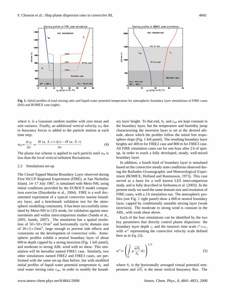
Fig. 1. Initial profiles of total mixing ratio and liquid water potential temperature for atmospheric boundary layer simulations of FIRE cases(left) and BOMEX case (right).

whereδi is a Gaussian random number with zero mean andunit variance. Finally, an additional vertical velocitywb dueto buoyancy forces is added to the particle motion at eachtime step:

wb=1zb

1t=

H (u, S, t+1t) −H (u, S, t)

1t(4)

The plume rise scheme is applied to each particle untilwb isless than the local vertical turbulent fluctuations.

2.3 Simulations set-up

The Cloud-Topped Marine Boundary Layer observed duringFirst ISCCP Regional Experiment (FIRE), at San NichollasIsland, 14–17 July 1987, is simulated with Meso-NH, usinginitial conditions provided by the EUROCS model compar-ison exercise (Duynkerke et al., 2004). FIRE is a well doc-umented experiment of a typical convective marine bound-ary layer, and a benchmark validation test for the atmo-spheric modelling community. It has been successfully simu-lated by Meso-NH in LES mode, for validation against mea-surements and within intercomparison studies (Sandu et al.,2005; Sandu, 2007). The simulation has a spatial resolu-tion of 50×50×10 m3 and horizontally cyclic domain sizeof 20×5×3 km3, large enough to prevent side effects andconstraints on the development of convective cells. Atmo-spheric profiles exhibit a neutral boundary layer of about600 m depth capped by a strong inversion (Fig. 1 left panel),and moderate to strong ABL wind with no shear. This sim-ulation will be hereafter named FIRE1 case. Similarly, twoother simulations named FIRE2 and FIRE3 cases, are per-formed with the same set-up than before, but with modifiedinitial profiles of liquid water potential temperatureθL andtotal water mixing ratiortot, in order to modify the bound-

ary layer height. To that end,θL andrtot are kept constant inthe boundary layer, but the temperature and humidity jumpcharacterizing the inversion layer is set at the desired alti-tude, above which the profiles follow the initial free tropo-sphere slope (Fig. 1 left panel). The resulting boundary layerheights are 400 m for FIRE2 case and 800 m for FIRE3 case.All FIRE simulation cases ran for one hour after 2 h of spin-up, in order to reach a fully developed, steady, well-mixedboundary layer.

In addition, a fourth kind of boundary layer is simulatedbased on the convective steady state conditions observed dur-ing the Barbados Oceanographic and Meteorological Exper-iment (BOMEX; Holland and Rasmusson, 1973). This caseserved as a basis for a well known LES intercomparisonstudy, and is fully described in Siebesma et al. (2003). In thepresent study we used the same domain size and resolution ofFIRE cases, with a 2 h simulation run. The atmospheric pro-files (see Fig. 1 right panel) show a 600 m neutral boundarylayer, capped by conditionally unstable mixing layer (weakinversion). The moderate to strong wind is constant in theABL, with weak shear above.

Each of the four simulations can be identified by the twokey parameters that directly control plume dispersion: theboundary layer depthzi and the turnover time scalet∗=zi ,with w∗ representing the convective velocity scale definedhere as in Eq. (5):

w∗=

zi∫0

gwθv

θv

dz

1/3

(5)

whereθv is the horizontally averaged virtual potential tem-perature andwθv is the mean vertical buoyancy flux. The

www.atmos-chem-phys.net/8/4841/2008/ Atmos. Chem. Phys., 8, 4841–4853, 2008


Table 1. Boundary layer depthzi and characteristic turn-over timescalet∗ of the simulated BL cases.

FIRE1 FIRE2 FIRE3 BOMEX

zi 580 400 800 600t∗(min) 22.2 12.3 29.2 23.5

values of these two parameters are presented in Table 1, andare used as scaling factors to characterize plume dispersion.

2.4 Simulating a characteristic plume

One major issue in the simulation of ship plumes – e.g. forvalidation of parameterizations or comparison with observa-tions – is that the shape of the plume strongly depends onthe local flow conditions around each particle trajectory. Forexample, the rise and fall of a plume are influenced by ex-tremely scattered and random events such as the updraftsand downdrafts occurring in a turbulent convective bound-ary layer. Besides, the exact values of the ship speed anddirection (relative to the wind) are generally unknown. Allthese uncertainties and the wide range of spatial and tempo-ral variability of the parameters make any single simulationof the plume a particular case among huge number of possi-ble combinations. On the other hand, simulation of all con-ceivable cases is obviously unaffordable. A reasonable com-promise made in this study is to reconstruct the propertiesof a generic (“idealized”) plume that is somehow representa-tive of any plume evolving in a given ABL. This done in twosteps as detailed next.

The first step is to consider that a plume is the superpo-sition of puffs released at different times and different loca-tions. The above mentioned generic plume model can thenbe treated using one single puff simulation. The second stepis to model such a puff – characteristic of the whole bound-ary layer – so as to get rid of the dependency on local time-changing dynamical events. The idea is to release a largenumber of particles equally distributed in space and eventu-ally in time at the same ship stack level over all the modeledboundary layer.

The time evolution of the normalized concentration fieldof this “generic puff”, characteristic of the given boundarylayer, can then be recombined from the particle positions attime t following (adapted from Lamb, 1978):

C (x, y, z, t) =

t∫−∞

Q(t ′)p1(xp (t) −x0−U×(t−t ′),

yp (t) −y0−V ×(t−t ′

), zp (t) , t ′

)dt ′ (6)

whereQ is the source strength function which can be timedependent;xp (t), yp (t) andzp (t) indicate the particle posi-tion at timet ; x0 andy0 indicate the initial particle position at

its release timet ′; U , V are horizontal mean wind speed com-ponents of the ABL in the case of a stationary source. In thecase of a moving source, (U, V ) can be interpreted as the rel-ative wind speed components (Uwind−Uship, Vwind−Vship).p1 is the position PDF for particles found at timet in a coor-dinate system that depends on the particle initial position andthe mean advection. The method is thus particularly suitablefor practical implementation in atmospheric chemistry mod-els which rely only on general boundary layer parameters.It must however be noted that Eq. (6) accurately describesany generic puff provided that the statistic properties of tur-bulence is independent enough from the mean wind velocity,which is the case in convective boundary layers but not forshear-driven boundary layers.

In our cases, the LES fields are stored every minute, pro-vided off-line to the Lagrangian model and interpolated intime and space (taking advantage of the cyclic boundary con-ditions of the LES domain); 50 000 particles are released in-stantaneously, equally distributed horizontally over the do-main, at an initial altitude of 60 m, matching the upper limitof ship height above sea level in international PANAMAXstandard for major marine vessels (which defines the maxi-mum size allowed for the crossing of the Panama Canal, andcorresponds to the design of modern container ships).

3 Analysis of plume dispersion parameters

3.1 Influence of ship stack buoyancy flux on plume disper-sion

The mean initial buoyancy flux at ship stackF (Eq. 2)is a tunable parameter for the puff dispersion simulation.The plume rise scheme is applied to each particle followingEq. (3). For each boundary layer case, seven plume sim-ulations are performed with a mean initial buoyancy fluxF=0 m4 s−3 (no buoyancy), 50, 100, 120, 150, 200 and250 m4 s−3.

Although the initial buoyancy flux can have a major im-pact on plume dispersion as discussed above, in situ obser-vations show that the heat and humidity release at ship stackcan not significantly raise the in-plume temperature and wa-ter mixing ratio above background level, even as close as200 m from the stack. In rare and specific cases, only a smalltemperature increase of less than 0.4◦K has been documented(Hobbs et al., 2000).

In the simulations, the temperature difference betweenplume and boundary layer background can be estimatedusing the plume rise scheme integrated in the Lagrangianmodel. For each particle and at each time step, a verticalbuoyancy acceleration is obtained by taking time derivativeof its plume rise velocitywb (t) defined in Eq. (4). This ac-celeration can be related to temperature difference between



the plume air particle and the surrounding environment via abuoyancy force:

∂wb

∂t=

1wb

1t≈g

θv−θvref

θvref(7)

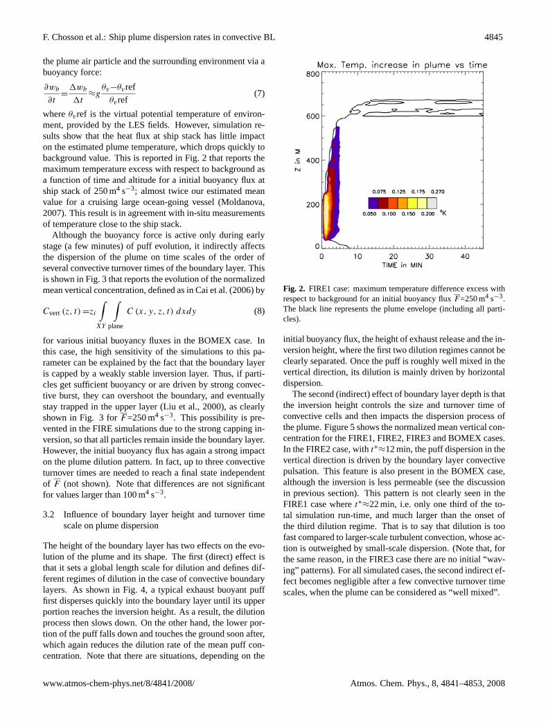
whereθvref is the virtual potential temperature of environ-ment, provided by the LES fields. However, simulation re-sults show that the heat flux at ship stack has little impacton the estimated plume temperature, which drops quickly tobackground value. This is reported in Fig. 2 that reports themaximum temperature excess with respect to background asa function of time and altitude for a initial buoyancy flux atship stack of 250 m4 s−3; almost twice our estimated meanvalue for a cruising large ocean-going vessel (Moldanova,2007). This result is in agreement with in-situ measurementsof temperature close to the ship stack.

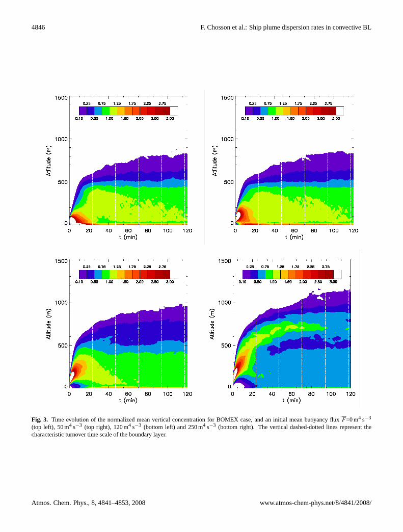
Although the buoyancy force is active only during earlystage (a few minutes) of puff evolution, it indirectly affectsthe dispersion of the plume on time scales of the order ofseveral convective turnover times of the boundary layer. Thisis shown in Fig. 3 that reports the evolution of the normalizedmean vertical concentration, defined as in Cai et al. (2006) by

Cvert (z, t) =zi

∫XY

∫plane

C (x, y, z, t) dxdy (8)

for various initial buoyancy fluxes in the BOMEX case. Inthis case, the high sensitivity of the simulations to this pa-rameter can be explained by the fact that the boundary layeris capped by a weakly stable inversion layer. Thus, if parti-cles get sufficient buoyancy or are driven by strong convec-tive burst, they can overshoot the boundary, and eventuallystay trapped in the upper layer (Liu et al., 2000), as clearlyshown in Fig. 3 forF=250 m4 s−3. This possibility is pre-vented in the FIRE simulations due to the strong capping in-version, so that all particles remain inside the boundary layer.However, the initial buoyancy flux has again a strong impacton the plume dilution pattern. In fact, up to three convectiveturnover times are needed to reach a final state independentof F (not shown). Note that differences are not significantfor values larger than 100 m4 s−3.

3.2 Influence of boundary layer height and turnover timescale on plume dispersion

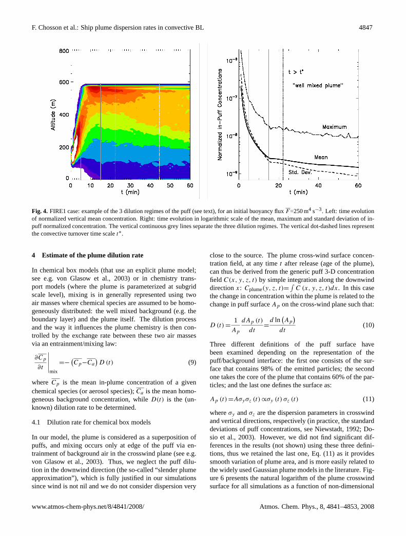
The height of the boundary layer has two effects on the evo-lution of the plume and its shape. The first (direct) effect isthat it sets a global length scale for dilution and defines dif-ferent regimes of dilution in the case of convective boundarylayers. As shown in Fig. 4, a typical exhaust buoyant pufffirst disperses quickly into the boundary layer until its upperportion reaches the inversion height. As a result, the dilutionprocess then slows down. On the other hand, the lower por-tion of the puff falls down and touches the ground soon after,which again reduces the dilution rate of the mean puff con-centration. Note that there are situations, depending on the

F. Chosson, R. Paoli and B. Cuenot, 2008: Ship plume dispersion rates in convective BL …

18 / 29

Figure 2. FIRE1 case: maximum temperature difference excess with respect to

background for an initial buoyancy flux F = 250m4.s-3. The black line

represents the plume envelope (including all particles).

Fig. 2. FIRE1 case: maximum temperature difference excess withrespect to background for an initial buoyancy fluxF=250 m4 s−3.The black line represents the plume envelope (including all parti-cles).

initial buoyancy flux, the height of exhaust release and the in-version height, where the first two dilution regimes cannot beclearly separated. Once the puff is roughly well mixed in thevertical direction, its dilution is mainly driven by horizontaldispersion.

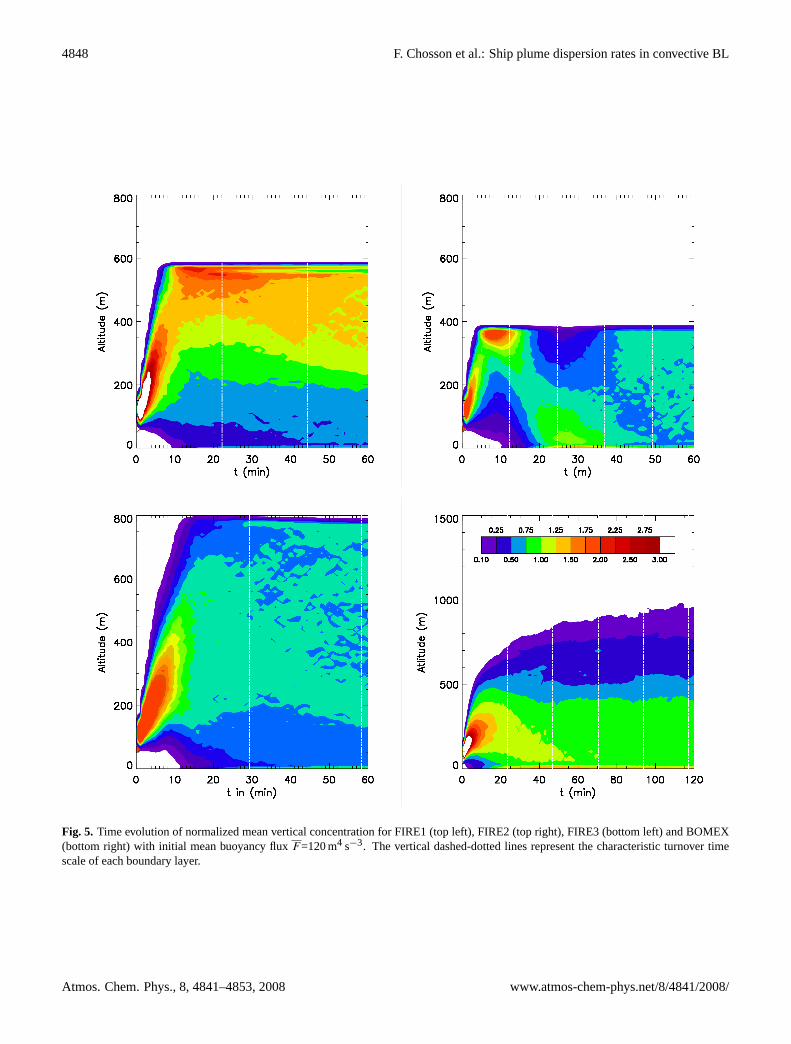
The second (indirect) effect of boundary layer depth is thatthe inversion height controls the size and turnover time ofconvective cells and then impacts the dispersion process ofthe plume. Figure 5 shows the normalized mean vertical con-centration for the FIRE1, FIRE2, FIRE3 and BOMEX cases.In the FIRE2 case, witht∗≈12 min, the puff dispersion in thevertical direction is driven by the boundary layer convectivepulsation. This feature is also present in the BOMEX case,although the inversion is less permeable (see the discussionin previous section). This pattern is not clearly seen in theFIRE1 case wheret∗≈22 min, i.e. only one third of the to-tal simulation run-time, and much larger than the onset ofthe third dilution regime. That is to say that dilution is toofast compared to larger-scale turbulent convection, whose ac-tion is outweighed by small-scale dispersion. (Note that, forthe same reason, in the FIRE3 case there are no initial “wav-ing” patterns). For all simulated cases, the second indirect ef-fect becomes negligible after a few convective turnover timescales, when the plume can be considered as “well mixed”.




19 / 29

Figure 3. Time evolution of the normalized mean vertical concentration for BOMEX case,

and an initial mean buoyancy flux F = 0 m4.s-3 (top left), 50 m4.s-3 (top right),

120 m4.s-3 (bottom left) and 250 m4.s-3 (bottom right). The vertical dashed-dotted

lines represent the characteristic turnover time scale of the boundary layer.

Fig. 3. Time evolution of the normalized mean vertical concentration for BOMEX case, and an initial mean buoyancy fluxF=0 m4 s−3

(top left), 50 m4 s−3 (top right), 120 m4 s−3 (bottom left) and 250 m4 s−3 (bottom right). The vertical dashed-dotted lines represent thecharacteristic turnover time scale of the boundary layer.




20 / 29

Figure 4. FIRE1 case: example of the 3 dilution regimes of the puff (see text), for an

initial buoyancy flux F = 250 m4.s-3. Left: time evolution of normalized

vertical mean concentration. Right: time evolution in logarithmic scale of the

mean, maximum and standard deviation of in-puff normalized concentration.

The vertical continuous grey lines separate the three dilution regimes. The

vertical dot-dashed lines represent the convective turnover time scale t*.

Fig. 4. FIRE1 case: example of the 3 dilution regimes of the puff (see text), for an initial buoyancy fluxF=250 m4 s−3. Left: time evolutionof normalized vertical mean concentration. Right: time evolution in logarithmic scale of the mean, maximum and standard deviation of in-puff normalized concentration. The vertical continuous grey lines separate the three dilution regimes. The vertical dot-dashed lines representthe convective turnover time scalet∗.

4 Estimate of the plume dilution rate

In chemical box models (that use an explicit plume model;see e.g. von Glasow et al., 2003) or in chemistry trans-port models (where the plume is parameterized at subgridscale level), mixing is in generally represented using twoair masses where chemical species are assumed to be homo-geneously distributed: the well mixed background (e.g. theboundary layer) and the plume itself. The dilution processand the way it influences the plume chemistry is then con-trolled by the exchange rate between these two air massesvia an entrainment/mixing law:

∂Cp

∂t

∣∣∣∣∣mix

=−(Cp−Ca

)D (t) (9)

where Cp is the mean in-plume concentration of a givenchemical species (or aerosol species);Ca is the mean homo-geneous background concentration, whileD(t) is the (un-known) dilution rate to be determined.

4.1 Dilution rate for chemical box models

In our model, the plume is considered as a superposition ofpuffs, and mixing occurs only at edge of the puff via en-trainment of background air in the crosswind plane (see e.g.von Glasow et al., 2003). Thus, we neglect the puff dilu-tion in the downwind direction (the so-called “slender plumeapproximation”), which is fully justified in our simulationssince wind is not nil and we do not consider dispersion very

close to the source. The plume cross-wind surface concen-tration field, at any timet after release (age of the plume),can thus be derived from the generic puff 3-D concentrationfield C(x, y, z, t) by simple integration along the downwinddirectionx: Cplume(y, z, t)=

∫C (x, y, z, t)dx. In this case

the change in concentration within the plume is related to thechange in puff surfaceAp on the cross-wind plane such that:

D (t) =1

Ap

dAp (t)

dt=

d ln(Ap

)dt

(10)

Three different definitions of the puff surface havebeen examined depending on the representation of thepuff/background interface: the first one consists of the sur-face that contains 98% of the emitted particles; the secondone takes the core of the plume that contains 60% of the par-ticles; and the last one defines the surface as:

Ap (t) =Aσyσz (t) ∝σy (t) σz (t) (11)

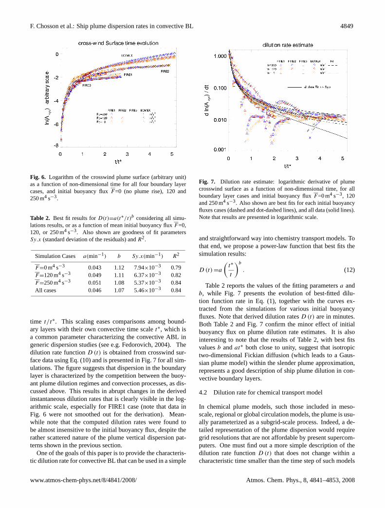
whereσy andσz are the dispersion parameters in crosswindand vertical directions, respectively (in practice, the standarddeviations of puff concentrations, see Niewstadt, 1992; Do-sio et al., 2003). However, we did not find significant dif-ferences in the results (not shown) using these three defini-tions, thus we retained the last one, Eq. (11) as it providessmooth variation of plume area, and is more easily related tothe widely used Gaussian plume models in the literature. Fig-ure 6 presents the natural logarithm of the plume crosswindsurface for all simulations as a function of non-dimensional




21 / 29

Figure 5. Time evolution of normalized mean vertical concentration for FIRE1 (top left),

FIRE2 (top right), FIRE3 (bottom left) and BOMEX (bottom right) with initial

mean buoyancy flux F = 120 m4.s-3. The vertical dashed-dotted lines represent

the characteristic turnover time scale of each boundary layer.

Fig. 5. Time evolution of normalized mean vertical concentration for FIRE1 (top left), FIRE2 (top right), FIRE3 (bottom left) and BOMEX(bottom right) with initial mean buoyancy fluxF=120 m4 s−3. The vertical dashed-dotted lines represent the characteristic turnover timescale of each boundary layer.




22 / 29

Figure 6. Logarithm of the crosswind plume surface (arbitrary unit) as a

function of non-dimensional time for all four boundary layer cases,

and initial buoyancy flux F = 0 (no plume rise), 120 and 250 m4.s-3.

Fig. 6. Logarithm of the crosswind plume surface (arbitrary unit)as a function of non-dimensional time for all four boundary layercases, and initial buoyancy fluxF=0 (no plume rise), 120 and250 m4 s−3.

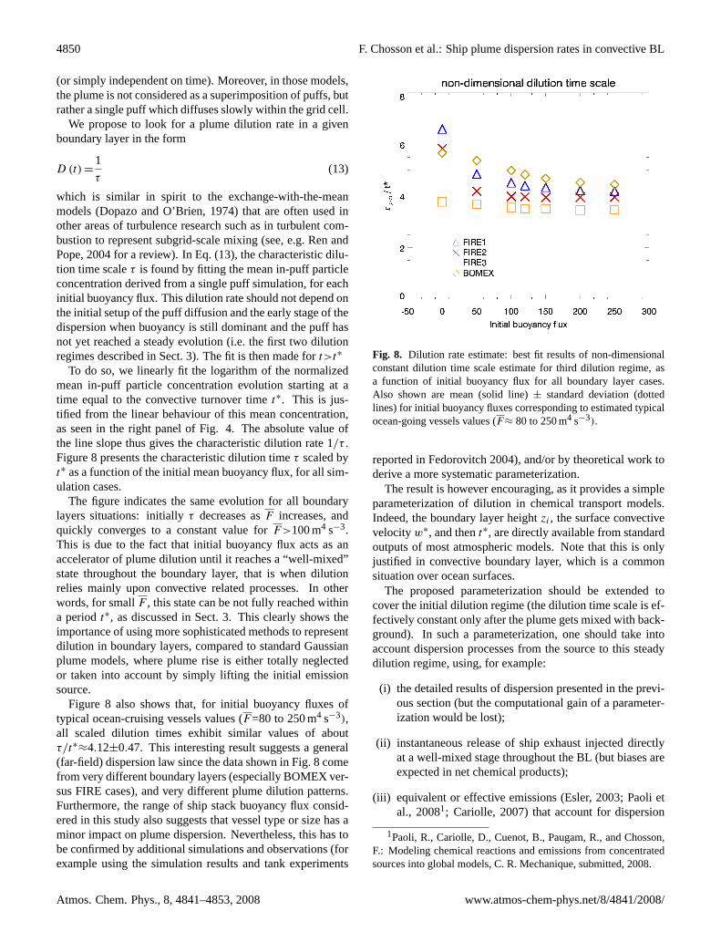
Table 2. Best fit results forD(t)=a(t∗/t)b considering all simu-lations results, or as a function of mean initial buoyancy fluxF=0,120, or 250 m4 s−3. Also shown are goodness of fit parametersSy.x (standard deviation of the residuals) andR2.

Simulation Cases a(min−1) b Sy.x(min−1) R2

F=0 m4 s−3 0.043 1.12 7.94×10−3 0.79F=120 m4 s−3 0.049 1.11 6.37×10−3 0.82F=250 m4 s−3 0.051 1.08 5.37×10−3 0.84All cases 0.046 1.07 5.46×10−3 0.84

time t/t∗. This scaling eases comparisons among bound-ary layers with their own convective time scalet∗, which isa common parameter characterizing the convective ABL ingeneric dispersion studies (see e.g. Fedorovich, 2004). Thedilution rate functionD (t) is obtained from crosswind sur-face data using Eq. (10) and is presented in Fig. 7 for all sim-ulations. The figure suggests that dispersion in the boundarylayer is characterized by the competition between the buoy-ant plume dilution regimes and convection processes, as dis-cussed above. This results in abrupt changes in the derivedinstantaneous dilution rates that is clearly visible in the log-arithmic scale, especially for FIRE1 case (note that data inFig. 6 were not smoothed out for the derivation). Mean-while note that the computed dilution rates were found tobe almost insensitive to the initial buoyancy flux, despite therather scattered nature of the plume vertical dispersion pat-terns shown in the previous section.

One of the goals of this paper is to provide the characteris-tic dilution rate for convective BL that can be used in a simple


23 / 29

Figure 7. Dilution rate estimate: logarithmic derivative of plume crosswind

surface as a function of non-dimensional time, for all boundary layer

cases and initial buoyancy flux F = 0 m4.s-3, 120 and 250 m4.s-3.

Also shown are best fits for each initial buoyancy fluxes cases

(dashed and dot-dashed lines), and all data (solid lines). Note that

results are presented in logarithmic scale.

Fig. 7. Dilution rate estimate: logarithmic derivative of plumecrosswind surface as a function of non-dimensional time, for allboundary layer cases and initial buoyancy fluxF=0 m4 s−3, 120and 250 m4 s−3. Also shown are best fits for each initial buoyancyfluxes cases (dashed and dot-dashed lines), and all data (solid lines).Note that results are presented in logarithmic scale.

and straightforward way into chemistry transport models. Tothat end, we propose a power-law function that best fits thesimulation results:

D (t) =a

(t∗

t

)b

. (12)

Table 2 reports the values of the fitting parametersa andb, while Fig. 7 presents the evolution of best-fitted dilu-tion function rate in Eq. (1), together with the curves ex-tracted from the simulations for various initial buoyancyfluxes. Note that derived dilution ratesD (t) are in minutes.Both Table 2 and Fig. 7 confirm the minor effect of initialbuoyancy flux on plume dilution rate estimates. It is alsointeresting to note that the results of Table 2, with best fitsvaluesb andat∗ both close to unity, suggest that isotropictwo-dimensional Fickian diffusion (which leads to a Gaus-sian plume model) within the slender plume approximation,represents a good description of ship plume dilution in con-vective boundary layers.

4.2 Dilution rate for chemical transport model

In chemical plume models, such those included in meso-scale, regional or global circulation models, the plume is usu-ally parameterized as a subgrid-scale process. Indeed, a de-tailed representation of the plume dispersion would requiregrid resolutions that are not affordable by present supercom-puters. One must find out a more simple description of thedilution rate functionD (t) that does not change within acharacteristic time smaller than the time step of such models



(or simply independent on time). Moreover, in those models,the plume is not considered as a superimposition of puffs, butrather a single puff which diffuses slowly within the grid cell.

We propose to look for a plume dilution rate in a givenboundary layer in the form

D (t) =1

τ(13)

which is similar in spirit to the exchange-with-the-meanmodels (Dopazo and O’Brien, 1974) that are often used inother areas of turbulence research such as in turbulent com-bustion to represent subgrid-scale mixing (see, e.g. Ren andPope, 2004 for a review). In Eq. (13), the characteristic dilu-tion time scaleτ is found by fitting the mean in-puff particleconcentration derived from a single puff simulation, for eachinitial buoyancy flux. This dilution rate should not depend onthe initial setup of the puff diffusion and the early stage of thedispersion when buoyancy is still dominant and the puff hasnot yet reached a steady evolution (i.e. the first two dilutionregimes described in Sect. 3). The fit is then made fort>t∗

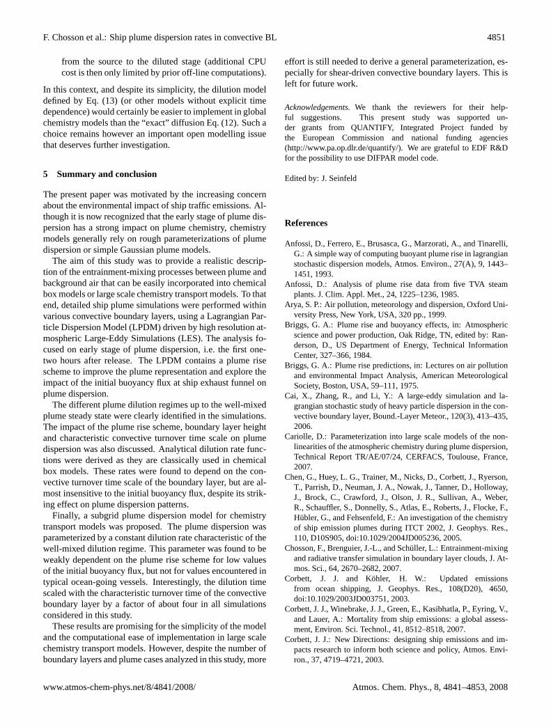
To do so, we linearly fit the logarithm of the normalizedmean in-puff particle concentration evolution starting at atime equal to the convective turnover timet∗. This is jus-tified from the linear behaviour of this mean concentration,as seen in the right panel of Fig. 4. The absolute value ofthe line slope thus gives the characteristic dilution rate 1/τ .Figure 8 presents the characteristic dilution timeτ scaled byt∗ as a function of the initial mean buoyancy flux, for all sim-ulation cases.

The figure indicates the same evolution for all boundarylayers situations: initiallyτ decreases asF increases, andquickly converges to a constant value forF>100 m4 s−3.This is due to the fact that initial buoyancy flux acts as anaccelerator of plume dilution until it reaches a “well-mixed”state throughout the boundary layer, that is when dilutionrelies mainly upon convective related processes. In otherwords, for smallF , this state can be not fully reached withina periodt∗, as discussed in Sect. 3. This clearly shows theimportance of using more sophisticated methods to representdilution in boundary layers, compared to standard Gaussianplume models, where plume rise is either totally neglectedor taken into account by simply lifting the initial emissionsource.

Figure 8 also shows that, for initial buoyancy fluxes oftypical ocean-cruising vessels values (F=80 to 250 m4 s−3),all scaled dilution times exhibit similar values of aboutτ/t∗≈4.12±0.47. This interesting result suggests a general(far-field) dispersion law since the data shown in Fig. 8 comefrom very different boundary layers (especially BOMEX ver-sus FIRE cases), and very different plume dilution patterns.Furthermore, the range of ship stack buoyancy flux consid-ered in this study also suggests that vessel type or size has aminor impact on plume dispersion. Nevertheless, this has tobe confirmed by additional simulations and observations (forexample using the simulation results and tank experiments


24 / 29

Figure 8. Dilution rate estimate: best fit results of non-dimensional constant

dilution time scale estimate for third dilution regime, as a function of

initial buoyancy flux for all boundary layer cases. Also shown are

mean (solid line) +/- standard deviation (dotted lines) for initial

buoyancy fluxes corresponding to estimated typical ocean-going

vessels values ( F ≈ 80 to 250 m4.s-3).

Fig. 8. Dilution rate estimate: best fit results of non-dimensionalconstant dilution time scale estimate for third dilution regime, asa function of initial buoyancy flux for all boundary layer cases.Also shown are mean (solid line)± standard deviation (dottedlines) for initial buoyancy fluxes corresponding to estimated typicalocean-going vessels values (F≈ 80 to 250 m4 s−3).

reported in Fedorovitch 2004), and/or by theoretical work toderive a more systematic parameterization.

The result is however encouraging, as it provides a simpleparameterization of dilution in chemical transport models.Indeed, the boundary layer heightzi , the surface convectivevelocityw∗, and thent∗, are directly available from standardoutputs of most atmospheric models. Note that this is onlyjustified in convective boundary layer, which is a commonsituation over ocean surfaces.

The proposed parameterization should be extended tocover the initial dilution regime (the dilution time scale is ef-fectively constant only after the plume gets mixed with back-ground). In such a parameterization, one should take intoaccount dispersion processes from the source to this steadydilution regime, using, for example:

(i) the detailed results of dispersion presented in the previ-ous section (but the computational gain of a parameter-ization would be lost);

(ii) instantaneous release of ship exhaust injected directlyat a well-mixed stage throughout the BL (but biases areexpected in net chemical products);

(iii) equivalent or effective emissions (Esler, 2003; Paoli etal., 20081; Cariolle, 2007) that account for dispersion

1Paoli, R., Cariolle, D., Cuenot, B., Paugam, R., and Chosson,F.: Modeling chemical reactions and emissions from concentratedsources into global models, C. R. Mechanique, submitted, 2008.



from the source to the diluted stage (additional CPUcost is then only limited by prior off-line computations).

In this context, and despite its simplicity, the dilution modeldefined by Eq. (13) (or other models without explicit timedependence) would certainly be easier to implement in globalchemistry models than the “exact” diffusion Eq. (12). Such achoice remains however an important open modelling issuethat deserves further investigation.

5 Summary and conclusion

The present paper was motivated by the increasing concernabout the environmental impact of ship traffic emissions. Al-though it is now recognized that the early stage of plume dis-persion has a strong impact on plume chemistry, chemistrymodels generally rely on rough parameterizations of plumedispersion or simple Gaussian plume models.

The aim of this study was to provide a realistic descrip-tion of the entrainment-mixing processes between plume andbackground air that can be easily incorporated into chemicalbox models or large scale chemistry transport models. To thatend, detailed ship plume simulations were performed withinvarious convective boundary layers, using a Lagrangian Par-ticle Dispersion Model (LPDM) driven by high resolution at-mospheric Large-Eddy Simulations (LES). The analysis fo-cused on early stage of plume dispersion, i.e. the first one-two hours after release. The LPDM contains a plume risescheme to improve the plume representation and explore theimpact of the initial buoyancy flux at ship exhaust funnel onplume dispersion.

The different plume dilution regimes up to the well-mixedplume steady state were clearly identified in the simulations.The impact of the plume rise scheme, boundary layer heightand characteristic convective turnover time scale on plumedispersion was also discussed. Analytical dilution rate func-tions were derived as they are classically used in chemicalbox models. These rates were found to depend on the con-vective turnover time scale of the boundary layer, but are al-most insensitive to the initial buoyancy flux, despite its strik-ing effect on plume dispersion patterns.

Finally, a subgrid plume dispersion model for chemistrytransport models was proposed. The plume dispersion wasparameterized by a constant dilution rate characteristic of thewell-mixed dilution regime. This parameter was found to beweakly dependent on the plume rise scheme for low valuesof the initial buoyancy flux, but not for values encountered intypical ocean-going vessels. Interestingly, the dilution timescaled with the characteristic turnover time of the convectiveboundary layer by a factor of about four in all simulationsconsidered in this study.

These results are promising for the simplicity of the modeland the computational ease of implementation in large scalechemistry transport models. However, despite the number ofboundary layers and plume cases analyzed in this study, more

effort is still needed to derive a general parameterization, es-pecially for shear-driven convective boundary layers. This isleft for future work.

Acknowledgements.We thank the reviewers for their help-ful suggestions. This present study was supported un-der grants from QUANTIFY, Integrated Project funded bythe European Commission and national funding agencies(http://www.pa.op.dlr.de/quantify/). We are grateful to EDF R&Dfor the possibility to use DIFPAR model code.

Edited by: J. Seinfeld

References

Anfossi, D., Ferrero, E., Brusasca, G., Marzorati, A., and Tinarelli,G.: A simple way of computing buoyant plume rise in lagrangianstochastic dispersion models, Atmos. Environ., 27(A), 9, 1443–1451, 1993.

Anfossi, D.: Analysis of plume rise data from five TVA steamplants. J. Clim. Appl. Met., 24, 1225–1236, 1985.

Arya, S. P.: Air pollution, meteorology and dispersion, Oxford Uni-versity Press, New York, USA, 320 pp., 1999.

Briggs, G. A.: Plume rise and buoyancy effects, in: Atmosphericscience and power production, Oak Ridge, TN, edited by: Ran-derson, D., US Department of Energy, Technical InformationCenter, 327–366, 1984.

Briggs, G. A.: Plume rise predictions, in: Lectures on air pollutionand environmental Impact Analysis, American MeteorologicalSociety, Boston, USA, 59–111, 1975.

Cai, X., Zhang, R., and Li, Y.: A large-eddy simulation and la-grangian stochastic study of heavy particle dispersion in the con-vective boundary layer, Bound.-Layer Meteor., 120(3), 413–435,2006.

Cariolle, D.: Parameterization into large scale models of the non-linearities of the atmospheric chemistry during plume dispersion,Technical Report TR/AE/07/24, CERFACS, Toulouse, France,2007.

Chen, G., Huey, L. G., Trainer, M., Nicks, D., Corbett, J., Ryerson,T., Parrish, D., Neuman, J. A., Nowak, J., Tanner, D., Holloway,J., Brock, C., Crawford, J., Olson, J. R., Sullivan, A., Weber,R., Schauffler, S., Donnelly, S., Atlas, E., Roberts, J., Flocke, F.,Hubler, G., and Fehsenfeld, F.: An investigation of the chemistryof ship emission plumes during ITCT 2002, J. Geophys. Res.,110, D10S905, doi:10.1029/2004JD005236, 2005.

Chosson, F., Brenguier, J.-L., and Schuller, L.: Entrainment-mixingand radiative transfer simulation in boundary layer clouds, J. At-mos. Sci., 64, 2670–2682, 2007.

Corbett, J. J. and Kohler, H. W.: Updated emissionsfrom ocean shipping, J. Geophys. Res., 108(D20), 4650,doi:10.1029/2003JD003751, 2003.

Corbett, J. J., Winebrake, J. J., Green, E., Kasibhatla, P., Eyring, V.,and Lauer, A.: Mortality from ship emissions: a global assess-ment, Environ. Sci. Technol., 41, 8512–8518, 2007.

Corbett, J. J.: New Directions: designing ship emissions and im-pacts research to inform both science and policy, Atmos. Envi-ron., 37, 4719–4721, 2003.


http://www.pa.op.dlr.de/quantify/


Cosma-Averseng, S., Flamant, C., Pelon, J., Palm, S. P., andSchwemmer, G. K.: The cloudy atmospheric boundary layerover the subtropical South Atlantic Ocean: airborne-spacebornelidar observations and numerical simulation, J. Geophys. Res.,108(D7), 4220, doi:10.1029/2002JD002368, 2003.

Davis, D. D., Grodzinsky, G., Kasibhatla, P., Crawford, J., Chen,G., Liu, S., Bandy, A., Thornton, D., Guan, H., and Sandholm,S.: Impact of ship emissions on marine boundary layer NOx andSO2 distributions over the Pacific basin, Geophys. Res. Lett., 28,235–238, 2001.

Dosio, A., Vila-Guereau de Arellano, J., Holtslag, A. A. M., andBuiltjes, P. J. H.: Dispersion of a passive tracer in buoyancyand shear-driven boundary layers, J. Appl. Meteorol., 42, 1116–1130, 2003.

Dopazo, C. and O’Brien, E. : An approach to autoignition of a tur-bulent mixture, Acta Astronautica, 1, 1239–1266, 1974.

Duynkerke, P. G., De Roode, S. R., Van Zanten, M. C., Calvo,J., Cuxart, J., Cheinet, S., Chlond, A., Grenier, H., Jonker, P.J., Kohler, M., Lenderink, G., Lewellen, D., Lappen, C.-L.,Lock, A. P., Moeng, C.-H., Muller, F., Olmeda, D., Piriou, J.-M., Sanchez, E., and Sednev, I.: Observations and simulationsof the diurnal cycle of the EUROCS stratocumulus case, Q. J. R.Meteorol. Soc., 604, 3269–3296, 2004.

Esler, J. G., Roelofs, G. J., Kolher, M. O., and O’Connor, F. M.: Aquantitative analysis of grid-related systematic errors in exidis-ing capacity and ozone production rates in chemistry transportmodels, Atmos. Chem. Phys., 4, 1781–1795, 2004,http://www.atmos-chem-phys.net/4/1781/2004/.

Esler, J. G.: An integrated approach to mixing sensitivities in tro-pospheric chemistry: a basis for the parameterization of subgrid-scale emissions for chemistry transport models, J. Geophys. Res.,108(D20), 4632, doi:10.1029/2003JD003627, 2003.

Eyring, V., Kohler, H. W., Lauer, A ., and Lemper, B.: Emis-sions from international shipping – 2: Impact of future technolo-gies on scenarios until 2050, J. Geophys. Res., 110, D17306,doi:10.1029/2004JD005620, 2005b.

Eyring, V., Kohler, H.W., van Aardenne, J., and Lauer, A.: Emis-sions from international shipping – 1: The last 50 years, J. Geo-phys. Res., 110, D17305, doi:10.1029/2004JD005619, 2005a.

Fedorovich, E.: Dispersion of passive tracer in the atmospheric con-vective boundary layer with wind shears: a review of laboratoryand numerical model studies, Meteorol. Atmos. Phys., 87, 3–21,2004.

Geoffroy, O., Brenguier, J.-L., and Sandu, I.: Relationship betweendrizzle rate, liquid water path and droplet concentration at thescale of a stratocumulus cloud system, Atmos. Chem. Phys. Dis-cuss., 8, 3921–3959, 2008,http://www.atmos-chem-phys-discuss.net/8/3921/2008/.

Gopalakrishnan, S. G., and Avissar, R.: An LES study of the im-pacts of land surface heterogeneity on dispersion in the convec-tive boundary layer, J. Atmos. Sci., 57, 352–371, 2000.

Hobbs, P. V., Garrett, T. J., Ferek, R. J., Strader, S. R., Hegg, A.,Frick, G. M., Hoppel, A., Gasparovic, R. F., Russell, L. M., John-son, D. W., O’Dowd, C., Durkee, P. A., Nielsen, K. E., and Innis,G.: Emissions from Ships with respect to their effects on clouds,J. Atmos. Sci., 57, 2570–2590, 2000.

Holland, J. Z. and Rasmusson, E. M.: Measurement of atmosphericmass, energy, and momentum budgets over a 500-kilometersquare of tropical ocean, Mon. Weather Rev., 101, 44–55, 1973.

Hurley, P. J. and Physick, W.: Lagrangian particle modeling ofbuoyant point sources: plume rise and entrapment under con-vective conditions, Atmos. Environ., 27, 1579–1584, 1993.

Hurley, P. J.: The air pollution model (TAPM) version 1: technicaldescription and examples, CSIRO Atmospheric Research Tech-nical Paper No. 55, 43 pp., 1999.

Lafore, J.-P., Stein, J., Bougeault, P., Ducrocq, V., Duron, J., Fis-cher, C., Hereil, P., Mascart, P., Masson, V., Pinty, J.-P., Redels-berger, J. L., Richard, E., and Vila-Guerau de Arellano, J.: TheMeso-NH atmospheric simulation system – Part 1: Adiabatic for-mulation and control simulations, Ann. Geophys., 16, 90–109,1998,http://www.ann-geophys.net/16/90/1998/.

Lamb, R. G.: A numerical simulation of dispersion from an elevatedpoint source in the convective planetary boundary layer, Atmos.Environ., 12, 1297–1304, 1978.

Liu, Q., Kogan, Y. L., Lilly, D. K., Johnson, D. W., Innis, G. E.,Durkee, P. A., and Nielsen, K. E.: Modeling of Ship effluenttransport and its sensitivity to boundary layer structure, J. Atmos.Sci., 57, 2779–2791, 2000.

Luhar, A. K. and Britter, R. E.: Random-walk modeling of buoyant-plume dispersion in the convective boundary layer, Atmos. Env-iron., 26, 1283–1298, 1992.

Mason, P. J.: Large-eddy simulation of dispersion in convectiveboundary layers with wind shear, Atmos. Environ., 26A, 1561–1571, 1992.

Moldanova, J.: Main campaign quicklooks and preliminary datafrom the ship exhaust measurements, QUANTIFY European In-tegrated Project, internal report no. D.2.3.2.10, 2007.

Nieuwstadt, F. T. M.: A Large-Eddy simulation of a line source ina convective atmospheric boundary layer – 1: Dispersion charac-teristics, Atmos. Envir., 26A, 485–495, 1992.

Pier Siebesma, A., Bretherton, C. S., Brown, A., Chlond, A.,Cuxart, J., Duynkerke, P. G., Jiang, H., Khairoutdinov, M.,Lewellen, D., Moeng, C.-H., Sanchez, E., Stevens, B., andStevens, D. E.: A Large Eddy Simulation Intercomparison Studyof Shallow Cumulus Convection, J. Atmos. Sci., 60, 10, 1201–1219, 2003.

Pingkuan, D., Servin, A., Rosenkranz, K., and Schwarh, B.: Dieselparticulate matter exposure assessment study for the ports of LosAngeles and Long Beach, California Environment ProtectionAgency, Air Ressources Board (ARB), Sacramento, CA, USA,74 pp., 2006.

Poppe, D., Koppmann, R., and Rudolph, J.: Ozone formation inbiomass burning plumes: Influence of atmospheric chemistry,Geophys. Res. Lett., 25, 3823–3826, 1998.

Ren, Z. and Pope, S. B. : An investigation of the performance ofturbulent mixing models, Comb. Flame, 136, 208–216, 2004.

Richter, A., Eyring, V., Burrows, J.P., Bovensmann, H., Lauer, A.,Sierk, B., and Crutzen, P. J.: Satellite measurements of NO2 frominternational shipping emissions, Geophys. Res. Lett., 31(23),L23110, doi:10.1029/2004GL020822, 2004.

Sandu, I., Tulet, P., and Brenguier, J.-L.: Parameterization of thecloud droplet single scattering albedo based on aerosol chem-ical composition for LES modeling of boundary layer clouds,Geophys. Res. Lett., 32, L19814, doi:10.1029/2005GL023994,2005.

Sandu, I.: Impact des aerosols sur le cycle de vie des nuages decouche limite, PhD Thesis, Meteo-France, Universite Toulouse


http://www.atmos-chem-phys.net/4/1781/2004/

http://www.atmos-chem-phys-discuss.net/8/3921/2008/

http://www.ann-geophys.net/16/90/1998/


III, France, 2007.Schlager, H., Baumann, R., Lichtenstern, M., Petzold, A., Arnold,

F., Speidel, M., Gurk, C., and Fischer, H.: Aircraft-based tracegas measurements in a primary European ship corridor, in: Pro-ceedings of the International Conference on Transport, Atmo-sphere and Climate (TAC), 26–29 June 2006, Oxford, UK, 83–88, 2006.

von Glasow, R., Lawrence, M. G., Sander, R., and Crutzen, P. J.:Modeling the chemical effects of ship exhaust in the cloud-freemarine boundary layer, Atmos. Chem. Phys., 3, 233–250, 2003,http://www.atmos-chem-phys.net/3/233/2003/.

Weil, J. C., Sullivan, P. P., and Moeng, C.-H.: The use of large-eddysimulations in Lagrangian particle dispersion models, J. Atmos.Sci., 61, 2877–2887, 2004.

Wendum, D.: Three long range transport models compared to theETEX experiment: a performance study, Atmos. Env., 32, 4297–4305, 1998.


http://www.atmos-chem-phys.net/3/233/2003/

Documents

Ship plume dispersion rates in convective boundary …cfdbib/repository/TR_CFD_08_124.pdf · The spatial and temporal evolution of ship plumes are sim- ... a stochastic LPDM based