Embed Size (px)
Citation preview
MATH 283A Topics in Topology
Shintaro Fushida-Hardy
381B Sloan Hall, Stanford University, CA
This document contains course notes from MATH 283A (taught at Stanford, spring 2020,by Ciprian Manolescu) transcribed by Shintaro Fushida-Hardy. Some additional thoughts
and mistakes may have been added.
Contents
1 Classification of 4-manifolds 31.1 Admin (lecture 1) . . . . . . . . . . . . . . . . . . . . . . . . . . . . . . . . . 31.2 The futility of a full classification of 4-manifolds . . . . . . . . . . . . . . . 41.3 The intersection form . . . . . . . . . . . . . . . . . . . . . . . . . . . . . . 61.4 Intersection form homotopy type? (lecture 2) . . . . . . . . . . . . . . . 81.5 Intersection form homeomorphism type? . . . . . . . . . . . . . . . . . . 91.6 Homeomorphism type diffeomorphism type? . . . . . . . . . . . . . . . . 101.7 Classification of symmetric Z-bilinear forms . . . . . . . . . . . . . . . . . . 121.8 Summary of homeomorphism types of X4 (lecture 3) . . . . . . . . . . . . . 141.9 Crash course on characteristic classes . . . . . . . . . . . . . . . . . . . . . . 151.10 Classifying homeomorphism types of X4 with characteristic classes . . . . . 171.11 Algebraic surfaces as smooth 4-manifolds . . . . . . . . . . . . . . . . . . . 18
2 Representations of 4-manifolds 222.1 Morse functions and handle decompositions (lecture 4) . . . . . . . . . . . . 222.2 Handle moves . . . . . . . . . . . . . . . . . . . . . . . . . . . . . . . . . . . 242.3 H-cobordism theorem . . . . . . . . . . . . . . . . . . . . . . . . . . . . . . 252.4 Handle decompositions of 3 and 4 manifolds (lecture 5) . . . . . . . . . . . 282.5 Kirby diagrams . . . . . . . . . . . . . . . . . . . . . . . . . . . . . . . . . . 292.6 Surgery diagrams (lecture 6) . . . . . . . . . . . . . . . . . . . . . . . . . . 332.7 Kirby calculus . . . . . . . . . . . . . . . . . . . . . . . . . . . . . . . . . . . 342.8 Heegaard diagrams . . . . . . . . . . . . . . . . . . . . . . . . . . . . . . . . 372.9 Trisections (lecture 7) . . . . . . . . . . . . . . . . . . . . . . . . . . . . . . 38
3 Construction of Seiberg-Witten gauge theory 413.1 Clifford modules . . . . . . . . . . . . . . . . . . . . . . . . . . . . . . . . . 413.2 Spinc structure definitions (lecture 8) . . . . . . . . . . . . . . . . . . . . . . 433.3 Spinc structure existence and classification . . . . . . . . . . . . . . . . . . . 443.4 Hodge theory . . . . . . . . . . . . . . . . . . . . . . . . . . . . . . . . . . . 463.5 Hodge meets spinc (lecture 9) . . . . . . . . . . . . . . . . . . . . . . . . . . 47
1
3.6 Connections and curvature . . . . . . . . . . . . . . . . . . . . . . . . . . . 493.7 Seiberg-Witten equations . . . . . . . . . . . . . . . . . . . . . . . . . . . . 523.8 Seiberg-Witten moduli space (lecture 10) . . . . . . . . . . . . . . . . . . . 533.9 Counting solutions to SW . . . . . . . . . . . . . . . . . . . . . . . . . . . . 543.10 The Seiberg-Witten invariant . . . . . . . . . . . . . . . . . . . . . . . . . . 56
4 Applications of Seiberg-Witten theory 584.1 Basic properties of SW (lecture 11) . . . . . . . . . . . . . . . . . . . . . . . 584.2 Basic applications of SW . . . . . . . . . . . . . . . . . . . . . . . . . . . . . 594.3 Proofs of the basic properties . . . . . . . . . . . . . . . . . . . . . . . . . . 614.4 Proof of the adjunction inequality for SW (lecture 12) . . . . . . . . . . . . 634.5 Resolving the Thom conjecture using SW . . . . . . . . . . . . . . . . . . . 674.6 Resolving the Milnor conjecture using SW . . . . . . . . . . . . . . . . . . . 684.7 Knots bounding affine algebraic curves (lecture 13) . . . . . . . . . . . . . . 694.8 Donaldson diagonalisability theorem . . . . . . . . . . . . . . . . . . . . . . 724.9 Infinitude of smooth structures on K3. . . . . . . . . . . . . . . . . . . . . . 744.10 Furuta’s 10/8-theorem (lecture 14) . . . . . . . . . . . . . . . . . . . . . . . 774.11 Exotic smooth structures on R4 . . . . . . . . . . . . . . . . . . . . . . . . . 80
5 Khovanov homology 835.1 Definition of Khovanov homology (lecture 15) . . . . . . . . . . . . . . . . . 835.2 Khovanov example: the right-handed trefoil . . . . . . . . . . . . . . . . . . 875.3 Isotopy invariance of Khovanov homology . . . . . . . . . . . . . . . . . . . 895.4 Generalising Khovanov homology: TQFTs (lecture 16) . . . . . . . . . . . . 915.5 Lee homology and spectral sequences . . . . . . . . . . . . . . . . . . . . . . 945.6 Rasmussen’s s-invariant (lecture 17) . . . . . . . . . . . . . . . . . . . . . . 975.7 The s-invariant bounds the slice genus . . . . . . . . . . . . . . . . . . . . . 1005.8 Combinatorial proof of Milnor’s conjecture (lecture 18) . . . . . . . . . . . . 1025.9 Combinatorial proof of the existence of exotic R4s . . . . . . . . . . . . . . 1045.10 FGMW strategy to disprove SPC4 . . . . . . . . . . . . . . . . . . . . . . . 1065.11 The FGMW strategy fails for Gluck twists (lecture 19) . . . . . . . . . . . . 1085.12 Combinatorial proof of the Thom conjecture . . . . . . . . . . . . . . . . . . 112
2
Chapter 1
Classification of 4-manifolds
1.1 Admin (lecture 1)
Topics in the course will include:
1. topological 4-manifolds: Freedman’s classification (without proof)
2. presentations of smooth 4-manifolds: Kirby diagrams, trisections;
3. spinc structures, the Dirac operator, the Seiberg-Witten equations;
4. applications of gauge theory: exotic smooth structures, Donaldson’s diagonalizabilitytheorem, the Thom and Milnor conjectures;
5. (time permitting) Khovanov homology and the combinatorial proofs of the Thomand Milnor conjectures.
There is no official textbook for the course, but the following resources could be useful:
Robert Gompf and Andras Stipsicz, “4-Manifolds and Kirby Calculus”
Alexandru Scorpan, “The Wild World of 4-manifolds”
John Morgan, “The Seiberg-Witten Equations and Applications to the Topology ofSmooth Four-Manifolds”
John Moore, “Lectures on the Seiberg-Witten Invariants”
Simon Donaldson and Peter Kronheimer, “The Geometry of Four-Manifolds”
Results from the following research articles will also be discussed:
Peter Kronheimer and Tomasz Mrowka, “The Genus of Embedded Surfaces in theProjective Plane”. Mathematical Research Letters. 1 (1994), 797–808,
3
Mikhail Khovanov, , “A categorification of the Jones polynomial”, Duke Mathemat-ical Journal, 101 (2000), 359–426
David Gay and Robion Kirby, “Trisecting 4-manifolds”, Geom. Topol. 20 (2016),3097-3132
Peter Lambert-Cole, “Bridge trisections in CP2 and the Thom Conjecture”, arXiv:1807.10131
Some highlights from the course are the following three results:
1. There exist smooth homeomorphic 4-manifolds which are not diffeomorphic.
2. The Thom conjecture, proved by Kronheimer and Mrowka in 1994: if Σ ⊂ CP2 is asmoothly embedded surface, and Σ represents an algebraic curve of degree d, thenthe genus of Σ is at least (d− 1)(d− 2)/2.
3. The Milnor conjecture, also proven by Kronheimer and Mrowka in the 90s: let Tp,qdenote the torus knot with p twists and q strands. Suppose Σ ⊂ B4 is a smoothlyand properly embedded surface, with ∂Σ = Σ ∩ ∂B4 = Tp,q. Then the genus of Σ isat least (p− 1)(q − 1)/2.
The original proofs of the above three results were analytic in nature. More precisely, theemployed gauge theory - specifically the Yang-Mills and Seiberg-Witten equations.
Newer proofs are referred to as “combinatorial” in the literature, but this is a misnomer.The newer methods are algebraic and topological, without using analysis. A very importanttool is Khovanov homology.
1.2 The futility of a full classification of 4-manifolds
The most fundamental and desired result is a classification of all 4-manifolds. Unfortu-nately, this is hopeless by combining the following two theorems:
Theorem 1.2.1 (Adyan-Rubin, 1955). There does not exist an algorithm which determineswhether a given presentation of a group yields the trivial group.
Theorem 1.2.2 (Markov, 60s). Given a finitely presented group G, there exists a smoothclosed 4-manifold X with π1(X) = G.
Therefore smooth closed 4-manifolds are at least as complicated as finitely presentedgroups. It follows that we cannot classify smooth closed 4-manifolds up to homotopy, letalone up to diffeomorphism.
Proof of Markov’s theorem. The proof proceeds in a few steps.
4
Step 1. Given any 4-manifolds X1 and X2, π1(X1#X2) = π1(X1) ∗ π1(X2). This fol-lows from Seifert-Van Kampen. Observe that
π1(Xi) = π1(Xi −B4) ∗π1(S3) π1(B4) = π1(Xi −B4).
Therefore
π1(X1#X2) = π1(X1 −B4) ∗π1(S3) π1(X2 −B4) = π1(X1) ∗ π1(X2).
Step 2. Write G = 〈g1, . . . , gn|r1, . . . , rm〉. Suppose N is the connected sum of n copies ofS1 × S3. Then by step 1, π1(N) = ∗ni=1Z = 〈g1, . . . , gn〉.
Step 3. Consider any relation rj . These are represented by a loop γi ⊂ N . Since anytwo loops have dimension 1, and 1 + 1 < 4 = dimN , by the transversality theorem we canchoose the rj to be pairwise disjoint embedded submanifolds.
Step 4. Surgery on loops: fix a loop γ ⊂ N representing a relation r. This has a tubularneighbourhood, homeomorphic to S1 ×B3. Then
∂(N − (S1 ×B3)) = S1 × S2 = ∂(B2 × S2).
Therefore the idea is to cut out S1 ×B3 and glue in B2 × S2;
N := (N − (S1 ×B3)) tS1×S2 (B2 × S2).
Once again we apply Seifert-Van Kampen. Writing N = (N − (S1×B3))tS1×S2 (S1×B3),we have
π1(N) = π1(N − (S1 ×B3)) ∗〈r〉 〈r〉 = π1(N − (S1 ×B3)).
Therefore we see that
π1(N) = π1(N − (S1 ×B3)) ∗〈r〉 1 = π1(N − (S1 ×B3))/〈〈r〉〉 = π1(N)/〈〈r〉〉.
Since all of the γi in step 3 were chosen to be disjoint, the above surgery can be carriedout simultaneously on all of the γi, giving a closed smooth manifold M with fundamentalgroup π1(N)/〈〈r1, . . . , rm〉〉 = G.
Question from class. Where does this proof fail in lower dimensions?
Answer. The surgery above required the use of a four manifold with trivial fundamentalgroup, and boundary S1 × S2. In three dimensions, one can show that there do not existmanifolds with trivial fundamental group and boundary S1 × S1 (e.g. by comparing thefirst Betti number of the manifold to that of the boundary).
5
1.3 The intersection form
We’ve observed that there is no hope of classifying all 4-manifolds, so instead we restrictto those with trivial fundamental group. What are all of the closed simply connectedsmooth manifolds of dimension 4 ? In this course we usually consider classifications up todiffeomorphism, but sometimes homeomorphism or homotopy are considered. Note thatevery simply connected manifold is orientable, so no generality is lost in assuming our4-manifolds are oriented.
Question from class. Will we ever equip X with a metric?
Answer. For the traditional set-up with Seiberg-Witten equations and other PDE methods,a metric is necessary. However, in newer methods such as Khovanov homology, a metric isnot required.
We now study some invariants of an arbitrary oriented simply connected closed smoothmanifold X.
First since X is connected, H0(X;Z) = Z. By the universal coefficient theorem forcohomology, it follows that H0(X) = Z. Since X is oriented, Poincare duality applies,from which we conclude that H4(X) = H4(X) = Z.
Next since π1(X) = 0, by Hurewicz’s theorem we know that H1(X) = 0. By theuniversal coefficient theorem we find that H1(X) = 0. By Poincare duality it follows thatH3(X) = H3(X) = 0.
Finally we investigate H2(X). By Poincare duality, it is isomorphic to its own dual.But by the universal coefficient theorem,
H2(X) = Hom(H2(X),Z)⊕ Ext(H1(X),Z) = Hom(H2(X),Z),
so H2(X) is a free Z-module. Thus H2(X) = H2(X) = Zr, where r = b2(X) is thesecond Betti number of X. By Hurewicz’s theorem, we also know that π2(X) = H2(X).In summary:
H0 = H0 = H4 = H4 = Z, π1 = H1 = H1 = H3 = H3 = 0, π2 = H2 = H2 = Zr.
Recall that the cohomology is equipped with a cup product, Hp(X)×Hq(X)→ Hp+q(X).For an arbitrary oriented simply connected smooth 4-manifold, inspecting the cohomologygroups above, the most interesting cup product should be that of H2.
Definition 1.3.1. The intersection form of X is the symmetric unimodular bilinear form
Q : H2(X;Z)×H2(X;Z)→ Z
induced from the cup product by Poincare duality.
6
Suppose we consider the intersection form with real coefficients instead of integralcoefficients. We find that the intersection form then contains less information. Why isthis? With real coefficients, unimodular bilinear forms are classified by rank and signature.That is, any two unimodular matrices sharing the same rank and signature are similar overR. If A is a unimodular matrix of rank r and signature p, then over R
A ∼ diag(1, . . . , 1)⊕ diag(−1, . . . ,−1),
where the first diagonal matrix has size p× p, and the second (r − p)× (r − p).To see that unimodular matrices are more difficult to classify over Z, we introduce an
invariant:
Definition 1.3.2. Let A : Zr×Zr → Z be a bilinear form. A is even if A(a, a) = 0 mod 2for all a ∈ Zr. Evidently parity is a similarity invariant.
Example. Consider the matrices
A =
(1 00 −1
), B =
(0 11 0
).
These are both rank 2 signature 1 matrices, hence similar over R. However, A is not evenwhile B is even, so they are not similar over Z.
Why do we call Q the intersection form? This follows from the following theorem:
Theorem 1.3.3. Let X be a smooth 4-manifold. Then any α ∈ H2(X;Z) is representedby [Σ] for some smoothly embedded surface Σ ⊂ X.
Proof. There is an isomorphism between equivalence classes of complex line bundles overX and H2(X;Z) defined by sending each bundle E to its first chern class c1(E). Thusfix any complex line bundle over X representing α, and consider a generic section of thebundle. Then the zero-set of the section defines a surface (which can be assumed to besmoothly embedded by transversality) that represents α.
In general this proof holds in codimension 2.
With this in mind, the intersection form Q can be thought of as taking two surfaceswhich are transverse and counting their signed intersections.
Remark. Recall that π2 = H2 in the case of simply connected 4-manifolds, so every classα ∈ H2 can be represented by the image of f : S2 → X. But hey, doesn’t this contradictthe Thom conjecture? The key here is that the image of f is an immersed submanifold,while the Thom conjecture concerns embedded submanifolds. The Thom conjecture is anspecial case of the minimum genus problem:
What is mingenus(Σ) : Σ embedded surface, [Σ] = α ∈ H2?
7
In the next lecture, we prove that the intersection form determines the homotopy typeof a simply connected 4-manifold.
Theorem 1.3.4 (Whitehead). Let X1, X2 be closed simply connected topological 4-manifolds.Then X1 is homotopy equivalent to X2 if and only if their intersection forms are similarover Z.
To end the lecture we look at some examples of 4-manifolds and their intersection forms.
Example. If X = S4, then Q = 0 (the empty matrix.)
If X = CP2 (with the complex orientation) then Q = (1).
If X = CP2 (the projective plane with the reverse orientation), then Q = (−1).
If X = S2 × S2, then Q is the anti-diagonal matrix adiag(1, 1).
The connected sum X1#X2 has intersection form QX1 ⊕QX2 .
Inspecting the above examples, we can extract some non-trivial facts.
1. There is no orientation reversing diffeomorphism CP2 → CP2, since QCP2 6= QCP2 .
2. Let Q1 denote the intersection form of CP2#CP2, and Q2 the intersection form ofS2×S2. Then Q1 = (1)⊕(−1), so it has the same rank and signature as Q2. It followsthat they are similar over R, so homology with real coefficients cannot distinguish
S2 × S2 from CP2#CP2. However, S2 × S2 and CP2#CP2 aren’t even homotopyequivalent, since their integral intersection forms have different parity.
1.4 Intersection form homotopy type? (lecture 2)
At the end of the previous lecture, we mentioned a theorem due to Whitehead:
Theorem 1.4.1 (Whitehead). Let X1, X2 be closed simply connected topological 4-manifolds.Then X1 is homotopy equivalent to X2 if and only if their intersection forms are similarover Z.
In other words, closed simply connected 4-manifolds are completely determined up tohomotopy by their intersection forms. We now give a proof sketch.
Proof. Observe that H2(X) ∼= H2(X −B4) ∼= π2(X −B4), so generators of H2(X) can berepresented by maps fi : S2 → X − B4, with i = 1, . . . , r = b2(X). Thus we can define amap
f :
r∨i=1
S2 → X −B4
8
which induces isomorphisms on H∗. By relative Hurewicz, f induces isomorphisms on π∗,and by Whitehead’s theorem (not this one - the usual one), f is a homotopy equivalence.It follows that X is homotopic to
(∨ri=1 S2
)th e4, where h is a map h : S3 →
∨ri=1 S2. It
remains to understand the map h.Claim: π3
(∨ri=1 S2
)= symmetric r × r matrices over Z. (Thus each h corresponds
to an intersection form Q.) The idea behind this correspondence is that each element [h] ofπ3(S2) can be represented by the “linking number” lk(L,L′) of loops L and L′ defined tobe the preimages of points x, x′ under the map h. This arises from the Pontryagin-Thomconstruction. More generally, for h : S3 →
∨ri=1 S2, we obtain a matrix Qij = lk(Li, L
′j) of
linking numbers corresponding to [h].
Question from class. Why did we use X−B4 instead of just X at the start of the proof?
Answer. We needed to kill H4 by excision.
1.5 Intersection form homeomorphism type?
It is natural to ask whether or not the intersection form restricts 4-manifolds any further.How much can we say about the homeomorphism type of a manifold if we know its in-tersection form? What can we say about its diffeomorphism type? This is answered by acelebrated theorem by Freedman, which earned him a Field’s medal.
Theorem 1.5.1 (Freedman, 1982). (a) For every unimodular symmetric bilinear form Q,there exists a topological simply connected closed 4-manifold X with QX = Q.
(b) If Q is even, X is unique up to homeomorphism.
(c) If Q is odd, there are exactly two homeomorphism types of such an X, and at mostone of them admits a smooth structure.
In particular, the following corollary is immediate by combining (b) and (c):
Corollary 1.5.2. If X is a priori a smooth manifold, then its homeomorphism type iscompletely determined by QX .
The above theorem shows that it may be possible to detect smoothability by usinginvariants. This is indeed the case, one such invariant being the Kirby–Siebenmann invari-ant for simply connected n-manifolds; KSX ∈ H4(X;Z/2). Whenever KSX is non-zero,X does not admit a smooth structure. It turns out that the intersection form affects theKirby–Siebenmann invariant. Suppose X is a 4-manifold. Whenever QX is even, KSXvanishes. Whenever QX is odd, KSX is either 0 or 1.
Example. By Freedman’s theorem, there exists a topological 4-manifold X with QX = (1)which is not smoothable. (This manifold is now denoted ∗CP2, since it is the one othersimply connected closed 4-manifold with the same intersection form as CP2.) One canshow that KSX = 1.
9
1.6 Homeomorphism type diffeomorphism type?
A question that has not been addressed above is the uniqueness of smooth structures thatmay exist on topological manifolds. This section is dedicated to studying diffeomorphismtypes of manifolds, given a homeomorphism type.
Definition 1.6.1. A smooth structure on a topological manifold X is a diffeomorphismequivalence class of smooth manifolds homeomorphic to X. If X is a priori equipped witha smooth structure, another smooth structure is said to be exotic if it doesn’t contain X.That is,
Xhomeo∼= X ′, X
diffeo
6∼= X ′.
Example. In dimensions at most 3, every topological manifold admits a uniquesmooth structure (Moise, 50s).
For n 6= 4, Rn admits a unique smooth structure. On the other hand, R4 hasuncountably many. (Donaldson, Gompf, Taubes etc, 80s).
If X4 is closed, it has at most countably many smooth structures. This is becauseevery smooth structure in 4 dimensions is uniquely determined by a piecewise linearstructure, but a closed manifold admits at most countably many finite simplicialcomplexes (and hence countably many piecewise linear structures). Note that aclosed 4-manifold admitting countably many smooth structures has been exhibited;
namely CP2#kCP2, for k ≥ 2 (due to Akhmedov-Park).
For n 6= 4, Xn admits finitely many smooth structures. A well known example isexotic spheres:
– n = 4: It is unknown how many smooth structures S4 admits.
– n = 1, 2, 3, 5, 6: Sn has a unique smooth structure.
– n = 7: S7 admits 28 smooth structures (including orientation).
In principle we can count the number of smooth structures on Sn for n ≥ 5, in whichcase it reduces to understanding homotopy groups.
Remark. An interesting “non-example” is whether or not exotic smooth structures existon the following manifolds:
S4,CP2,CP2#CP2, S2 × S2.
The idea is that increasing topological complexity (Betti numbers) allows more space forconstructions, making it easier to find exotic structures.
In fact, a remarkable open question is the following:
10
Open question. Does every closed smooth 4-manifold admit infinitely many smooth struc-tures?
That is, we have not yet exhibited a single closed 4-manifold admitting only finitelymany smooth structures. A more familiar open problem is the last remaining open versionof the Poincare conjecture:
Conjecture. Every homotopy 4-sphere necessarily diffeomorphic to S4. Here after wedenote this conjecture by SPC4 (smooth Poincare conjecture, dimension 4).
By Freedman’s theorem, every homotopy 4-sphere is homeomorphic to a 4-sphere.Therefore the above question boils down to figuring out whether or not spheres admitexotic smooth structures. Two families of potential counter-examples to SPC4 will now bedescribed.
Example. The first family of potential counter examples are constructed via surgery usingbalanced presentations of the trivial group. In other words, presentations P = 〈g1, . . . , gm |r1, . . . , rm〉 (so the number of generators and relations is equal). Then XP is the simplyconnected manifold obtained from #m(S1 × S3) via surgery along loops, as in the con-struction in lecture 1 (where we proved that every finitely presented group arises as thefundamental group of a closed 4-manifold.)
We know that π1(XP ) = 0, while H1 = H3 = 0 and H0 = H4 = Z. Therefore to provethat XP is a homotopy sphere, it remains to show that H2 = 0. Suppose we know that theEuler characteristic of XP is 2. But
2 = χ(XP ) = 1− 0 + b2 − 0 + 1 = 2 + b2,
so this proves that H2 = 0. It turns out that (from the fact that P is balanced) we candeduce that χ(XP ) = 2. (See homework.) It follows from Freedman’s theorem that XP ishomeomorphic to the 4-sphere, but it’s unknown what the diffeomorphism type of XP is.
Some examples of balanced presentations of the trivial group are
P = 〈x, y | x4y3 = y2x2, x6y4 = y3x3〉, P ′ = 〈x, y | x4 = y5, xyx = yxy〉.
It is currently open whether or not XP is diffeomorphic to the sphere, while XP ′ wasfamously shown to be diffeomorphic to the sphere 8 years ago.
Example. The second family of potential counter examples is constructed using Glucktwists. (Again, see the homework.) The idea is to consider knotted embeddings S2 ∼= Σ→S4. Let V be a neighbourhood of Σ, diffeomorphic to S2 ×D2. Now consider the manifold
GΣ = (S4 − V ) tϕ (S2 ×D2),
where ϕ : S2×S1 → S2×S1 is a Gluck twist : ϕ(x, θ) = (rotθ(x), θ). It is left as an exerciseto prove that H2(GΣ) = 0, so that GΣ is homeomorphic to S4.
11
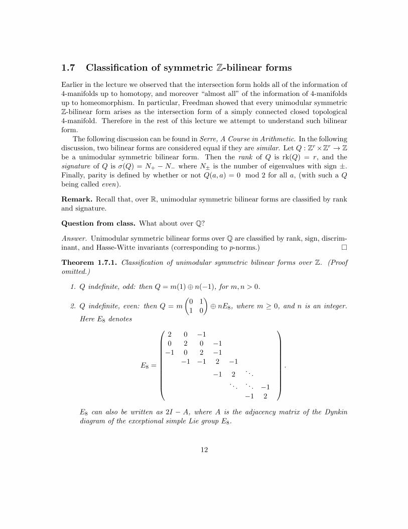
1.7 Classification of symmetric Z-bilinear forms
Earlier in the lecture we observed that the intersection form holds all of the information of4-manifolds up to homotopy, and moreover “almost all” of the information of 4-manifoldsup to homeomorphism. In particular, Freedman showed that every unimodular symmetricZ-bilinear form arises as the intersection form of a simply connected closed topological4-manifold. Therefore in the rest of this lecture we attempt to understand such bilinearform.
The following discussion can be found in Serre, A Course in Arithmetic. In the followingdiscussion, two bilinear forms are considered equal if they are similar. Let Q : Zr×Zr → Zbe a unimodular symmetric bilinear form. Then the rank of Q is rk(Q) = r, and thesignature of Q is σ(Q) = N+ − N− where N± is the number of eigenvalues with sign ±.Finally, parity is defined by whether or not Q(a, a) = 0 mod 2 for all a, (with such a Qbeing called even).
Remark. Recall that, over R, unimodular symmetric bilinear forms are classified by rankand signature.
Question from class. What about over Q?
Answer. Unimodular symmetric bilinear forms over Q are classified by rank, sign, discrim-inant, and Hasse-Witte invariants (corresponding to p-norms.)
Theorem 1.7.1. Classification of unimodular symmetric bilinear forms over Z. (Proofomitted.)
1. Q indefinite, odd: then Q = m(1)⊕ n(−1), for m,n > 0.
2. Q indefinite, even: then Q = m
(0 11 0
)⊕ nE8, where m ≥ 0, and n is an integer.
Here E8 denotes
E8 =
2 0 −10 2 0 −1−1 0 2 −1
−1 −1 2 −1
−1 2. . .
. . .. . . −1−1 2
.
E8 can also be written as 2I − A, where A is the adjacency matrix of the Dynkindiagram of the exceptional simple Lie group E8.
12
3. Q definite: complicated (whether or not Q is even or odd). For example, E16 can beinvolved.
Thus when Q is indefinite, it is determined uniquely by parity, rank, and signature. How-ever, when Q is definite, this no longer holds: for example, 9(1) is not similar to E8⊕ (1),but they are both odd, with rank and signature 9.
Which Q appears as QX for a closed simply connected topological 4-manifold? ByFreedman’s theorem, all of them do. What if X is smooth?
Theorem 1.7.2 (Rokhlin, 1952). If X is smooth and simply connected, with QX even,then 16 | σ(QX).
This is non-trivial. From algebraic arguments (using the classification above) we canonly conclude that 8 divides the signature of QX .
Corollary 1.7.3. There exists an “E8-manifold”, i.e. a simply connected closed topological4-manifold X with QX = E8, and this is not smoothable.
What about the 4-manifold corresponding to E8 ⊕ E8? This time 16 divides the sig-nature, but in fact it is still not smoothable! This is a corollary of the following ground-breaking result due to Donaldson, which was part of a wave of physical methods flowinginto maths.
Theorem 1.7.4 (Donaldson diagonalizability theorem, 1982). Let X4 be a smooth closedsimply connected manifold. Then if QX is definite, it is diagonalizable (over Z). That is,QX = ±r(1).
The original proof used the Yang-Mills equations. Newer proofs used Seiberg-Wittentheory, and even more recently Heegard-Floer homology. How about indefinite forms, ofwhich we have a better classification?
1. ForQ indefinite and odd, QX = m(1)⊕n(−1) is realised byX = (#mCP2)#(#nCP2).
2. For Q indefinite and even, we see later that for |m| ≤ (2/3)n, QX = n
(0 11 0
)⊕mE8
is realised by X being a connected sum of K3 surfaces and copies of S2×S2. A special
case is QX = 3
(0 11 0
)⊕ 2E8, which is realised by the Fermat quartic,
X = z40 + z4
1 + z42 + z4
3 = 0 ⊂ CP3.
The above restriction that |m| ≤ (2/3)n is quite curious. However, there is a conjecturethat this is not a restriction at all!
Conjecture (11/8-conjecture (Matsumoto)). If X is a simply connected closed smooth4-manifold, then we necessarily have that |m| ≤ (2/3)n.
Note that b2 = 2n + 8|m|, and σ = −8m, so the condition that |m| ≤ (2/3)n isequivalent to the condition that b2 ≥ (11/8)|σ|. This explains the naming.
13
1.8 Summary of homeomorphism types of X4 (lecture 3)
Recall the 11/8-conjecture from the previous lecture:
Conjecture (11/8-conjecture (Matsumoto)). If X is a simply connected closed smooth4-manifold, then we necessarily have b2 ≥ (11/8)|σ|.
Using Seiberg-Witten theory, a slightly weaker version of the conjecture has been knownfor several years:
Theorem 1.8.1 (10/8-theorem (Furuta)). If X is a simply connected closed smooth 4-manifold, then we necessarily have b2 ≥ (10/8)|σ|.
The 10/8-theorem is equivalent to the statement that |m| ≤ n, where m and n are asin the classification of Z-bilinear forms from the previous lecture. Most recently, a slightimprovement to the 10/8-theorem was achieved:
Theorem 1.8.2 (Hopkins, Lin, Shi, Xu). If X is a simply connected closed smooth 4-manifold, with m = 2p ≥ 4, then
n ≥
2p+ 2 p ≡ 1, 2, 5, 6
2p+ 3 p ≡ 3, 4, 7
2p+ 4 p ≡ 0
mod 8.
Here we can assume m is even by Rokhlin’s theorem. In fact, it was shown that this is thebest bound that can be achieved using Seiberg-Witten theory.
Summarising results so far, we have established the following:
Theorem 1.8.3. Let X4 be a simply connected closed smooth 4-manifold. Then the home-omorphism type of X is determined uniquely by
σ(QX), parity(QX), χ(X).
This follows from Freedman’s theorem, Donaldson’s diagonalisability theorem, and the clas-sification of symmetric unimodular Z-bilinear forms.
Equivalently, X is determined up to homeomorphism by b+2 , b−2 , and the parity of Q,
where b2 = b+2 + b−2 is the second Betti number of X, and b+2 is the number of positiveeigenvalues of QX , while b−2 is the number of negative eigenvalues. Then σ = b+2 − b
−2 and
χ = 2 + b2.
14
1.9 Crash course on characteristic classes
Using characteristic classes, it is possible to calculate σ(QX) and χ(X) in some cases. Firstwe define the four characteristic classes.
Definition 1.9.1 (Chern class). Let E → X be a complex vector bundle with rank r.(X can be any paracompact topological space, but is typically a manifold.) Then for eachk ∈ N, ck(E) ∈ H2k(X;Z) is uniquely determined by the following four properties:
1. Rank. c0(E) = 1, ck(E) = 0 for k > r.
2. Functoriality. If f : Y → X, then f∗ck(E) = ck(f∗E).
3. Product. If E,F → X, then c(E ⊕ F ) = c(E) ^ c(F ). Here c is the total Chernclass, c(E) = c0(E) + c1(E) + · · · ∈ H∗(X;Z). Thus for each k,
ck(E ⊕ F ) =
k∑i=0
ci(E) ^ ck−i(F ).
4. Normalisation. If X = CPn and E = TX, then c(E) = (1 + ω)n+1, where ω ∈H2(CPn) = Z is the Poincare dual of CPn−1 ⊂ CPn.
Geometrically, the chern class ck corresponds to the Poincare dual of the locus wherer + 1− k generic sections of E are linearly dependent. The Chern class enjoys a few morenotable properties:
Lemma 1.9.2. Let E → X be a complex vector bundle as above. Then
1. c1(E) = c1(ΛrE). The line bundle ΛrE → X is also denoted detE → X.
2. If L1, L2 → X are line bundles, then c1(L1 ⊗ L2) = c1(L1) + c1(L2).
3. For each k, ck(E∗) = (−1)kck(E), where E∗ is the dual bundle.
Next we define the Stiefel-Whitney classes. These are the real analogue of Chern classes.Every complex structure induces an orientation so integral homology was used above, butfor Stiefel-Whitney classes we use mod 2 homology.
Definition 1.9.3 (Stiefel-Whitney class). Let E → X be a real vector bundle with rankr. Then for each k ∈ N, wk(E) ∈ Hk(X;Z/2Z) is uniquely determined by the followingfour properties:
1. Rank. w0(E) = 1, wk(E) = 0 for k > r.
2. Functoriality. If f : Y → X, then f∗wk(E) = wk(f∗E).
15
3. Product. If E,F → X, then w(E ⊕ F ) = w(E) ^ w(F ). Here w is the totalStiefel-Whitney class, defined analogously to above.
4. Normalisation. If X = RPn and E = TX, then w(E) = (1 + ω)n+1, where ω ∈H2(RPn;Z/2Z) is the Poincare dual of RPn−1 ⊂ RPn.
In addition, we have the following properties.
Lemma 1.9.4. Let E → X be a real vector bundle as above. Then
1. Suppose E is endowed with a complex structure. Then w2k+1(E) = 0 for each k, andw2k(E) = ck(E) mod 2.
2. w1(E) = 0 if and only if E is orientable.
3. If w1(E) = 0, then w2(E) = 0 if and only if E is spinnable. We now explain whatthis means: oriented real vector bundle of rank r are in bijective correspondence withprincipal SO(r)-bundles, with a correspondence given by clutching maps. But SO(r)has a double cover, namely Spin(r) → SO(r). For r ≥ 3, since π1(SO(r)) = Z/2Z,Spin(r) is in fact the universal cover of SO(r). A spin structure on E is a lift of E toa Spin(r)-bundle.
The third characteristic class is again defined for real vector bundles, but via a com-plexification.
Definition 1.9.5 (Pontryagin class). Let E → X be a real vector bundle with rank r.Then for each k,
pk(E) = (−1)kc2k(E ⊗R C) ∈ H4k(X;Z).
Lemma 1.9.6. The Pontryagin class inherits rank, functoriality, product, and normalisa-tion properties from the Chern class.
The complex vector bundle E⊗RC→ X is called the complexification of E. Since thisis self-dual, by a property of the Chern class above, 2ck(E ⊗ C) = 0 for each odd k. Thuswe only consider even Chern classes in the definition of the Pontryagin class. The finalcharacteristic class is in fact the most familiar, as it relates directly to Euler characteristics.
Definition 1.9.7 (Euler class). Let E → X be an oriented real vector bundle of rank r.Then e(E) ∈ Hr(X;Z) is uniquely determined by the following properties:
1. Orientation. If E is E equipped with the opposite orientation, then e(E) = −e(E).
2. Functoriality. If f : Y → X is orientation preserving, then f∗e(E) = e(f∗E).
3. Product. If E,F → X are oriented, then e(E ⊕ F ) = e(E) ^ e(F ).
4. Normalisation. If E possesses a nowhere-vanishing section, then e(E) = 0.
16
Geometrically, the Euler class is the Poincare dual of the zero set of a generic sectionof E. In addition, we have the following properties.
Lemma 1.9.8. Let E → X be a real oriented vector bundle as above. Then
1. wr(E) = e(E) mod 2.
2. If E is endowed with a complex structure, e(E) = cr/2(E). In particular, pr/2(E) =cr(E ⊗R C) = e(E) ^ e(E).
3. If X is oriented, then choosing E = TX gives e(TX)[X] = χ(X), where χ(X) is theEuler characteristic.
1.10 Classifying homeomorphism types of X4 with charac-teristic classes
Suppose X4 is a simply connected closed smooth 4-manifold. In this section we show thatthe homeomorphism type of X is determined completely by the characteristic classes of X.(Specifically the Stiefel-Whitney, Pontryagin, and Euler class.) We also try to determineas much as we can about the characteristic classes, given the premise for X.
First we study the Euler class. Since X is orientable as shown in lecture 1, we assumeX is oriented. Then e(X) is determined entirely by the Euler characteristic χ(X) and viceversa.
Next we study the Pontryagin class. Since pi(TX) ∈ H4i(X;Z) and p0(TX) = 1, theonly non-trivial Pontryagin class is p1(TX). By the Hirzebruch signature theorem, we knowthat L1(X)[X] = σ(X) where L1(X) is the first L-class of X. But L1(X) = 1
3p1(TX), so itfollows that p1(TX)[X] = 3σ(X). Thus the first Pontryagin class is completely determinedby the signature σ(X) and vice versa.
Finally we investigate the Stiefel-Whitney classes. We know that wi(TX) ∈ H i(X;Z/2Z),and w0(TX) = 0 since X is oriented. How about w2 ∈ H i(X;Z/2Z)?
Lemma 1.10.1. w2(TX) is a characteristic element of X, i.e. 〈w2, α〉 = 〈α, α〉 mod 2 forall α ∈ H2(X;Z).
Proof. Let α ∈ H2(X;Z). From lecture 1, α is represented by an embedded orientedsurface, i.e. α is the Poincare dual [Σ], where Σ → X is a smooth oriented embedding.But TX|Σ = TΣ⊕NΣ, and on each of these we have w(TΣ) = 1 +w2(TΣ) and w(NΣ) =1 + w2(NΣ) (since all higher wk vanish). Thus by the product axiom
w(TX)|Σ = (1 + w2(TΣ))(1 + w2(NΣ)).
It follows that w2(TX) = w2(TΣ) + w2(NΣ). In particular, pairing with α gives
〈w2(TX), α〉 = w2(TΣ)[Σ] + w2(NΣ)[Σ] = e(TΣ)[Σ] + e(NΣ)[Σ] mod 2.
17
The last equality applies; we know that TΣ and NΣ are oriented since Σ and X areoriented. But (TΣ)[Σ] is the Euler characteristic of Σ, which vanishes mod 2. On theother hand, e(NΣ)[Σ] = 〈[Σ], [s(Σ)]〉 where s is a section of NΣ transverse to the zerosection. But then s(Σ) is itself a representative of α, so in summary
〈w2(TX), α〉 = e(NΣ)[Σ] = 〈α, α〉 mod 2.
Corollary 1.10.2. With X as above, QX is even if and only if TX is spinnable.
Proof. QX is even if and only if 〈α, α〉 = 0 mod 2 for all α ∈ H2(X;Z). But by theabove lemma, w2(TX) is a characteristic element, so equivalently QX is even if and onlyif 〈w2(TX), α〉 = 0 mod 2 for all α. Since QX is non-degenerate, this holds if and only ifw2(TX) vanishes, i.e. exactly when TX is spinnable.
In summary, the data of e(TX) is equivalent to that of the Euler characteristic of X,the data of p1(TX) is equivalent to that of the signature of QX , and the data of w2(TX)is equivalent to that of the parity of QX . Therefore we have the following:
Corollary 1.10.3. Let X be a closed simply connected smooth 4-manifold. Then theclasses e(X), p1(TX), and w2(TX) determine X up to homeomorphism.
1.11 Algebraic surfaces as smooth 4-manifolds
To finish this lecture we explore some examples of smooth 4-manifolds for which we cancompute characteristic classes. Namely, these are algebraic surfaces. Specifically, we con-sider
Zd = [z0 : · · · : z3] ∈ CP3 : P (zi) = 0,
where P is a homogeneous degree d polynomial, and the system of equations ∂P/∂zi =P = 0, i has no non-zero solutions. Then Zd is a smooth manifold. In fact, the diffeomor-phism type of Zd depends only on d and not on P . For example, we can always chooseP = zd0 + · · · + zd3 . (This is a homework problem.) Concretely, for each d, we have thefollowing:
1. Z1 = CP2 ⊂ CP3. This is automatic because P is a linear equation.
2. Z2 = CP1 × CP1 ∼= S2 × S2. We can choose our polynomial to be xy = uv. Then adiffeomorphism Z2 → CP1 × CP1 is given by [x : y : u : v] 7→ ([x : u], [y : v]).
3. Z3 = CP2#6CP2. This is a homework problem.
4. Z4 is a K3 surface. These are all diffeomorphic, but algebraically distinct.
18
5. Zd for d ≥ 5 are all “surfaces of general type”.
We now compute some characteristic classes associated to the Zd above. First by applyingthe Veronese embedding and Lefschetz hyperplane theorem, we conclude that Zd is simplyconnected. Write X = Zd, and X = CP3 ∩ V ⊂ CPm where V is some hyperplane, andCPm is the codomain of the Veronese embedding.
Let H → CP3 be the hyperplane line bundle, i.e. the dual bundle of the tautologicalbundle. We study characteristic classes of this bundle to better understand X. We beginwith Chern classes. First define
h = c1(H) = PD(CP2) ∈ H2(CP3) = Z.
Here PD(CP2) denotes the Poincare dual of [CP2]. Now consider X ⊂ CP3. Its normalbundle is given by H⊗d|X , so
c1(NX) = c1(H⊗d)|X = dη,
where η = h|X ∈ H2(X;Z). It follows that
c(TCP3|X) = c(TX)c(NX) = (1 + c1(TX) + c2(TX))(1 + dη).
On the other hand,c(TCP3|X) = (1 + η)4 = 1 + 4η + 6η2
by the normalisation axiom. Solving the system of equations gives
c1(TX) = (4− d)η, c2(TX) = (d2 − 4d+ 6)η2.
Next we can use the Chern classes to determine the Euler characteristic. Specifically, wehave
χ(X) = e(TX)[X] = c2(TX)[X] = (d2 − 4d+ 6)(η2[X]).
But η2[X] = d, because h[X] = d in CP3. This gives
χ(X) = d3 − 4d2 + 6d,
which also determines all Betti numbers of X (since we already knew all Betti numbersother than b2).
Next we determine the signature of QX . Recall that σ(QX) = 13p1(TX)[X]. But the
Pontryagin class is defined using the Chern classes which we have already understood!Specifically,
p1(TX) = −c2(TX ⊗ C) = −c2(TX ⊕ T ∗X) =
2∑i=0
ci(TX) ^ c2−i(T∗X).
19
Since ci(TX) = (−1)ici(T∗X), this gives p1(TX) = c2
1(TX) − 2c2(TX). (Note that thiscalculation holds for all complex algebraic surfaces!) In particular, we now find that thesignature is given by
σ(X) =d(4− d2)
3.
Finally, we determine the Stiefel-Whitney classes. Since w2 = c1 mod 2, we find that Qis even if and only if d is even. In summary, we have the following results:
Proposition 1.11.1. Let Zd be as above. Let Q denote its intersection form. Then theparity of Q is the parity of d, and
χ(Zd) = d3 − 4d2 + 6d, σ(Q) =d(4− d2)
3.
One can verify that Zd agrees with the 11/8-conjecture.
Example. We now fix d = 4. Then X = Z4 is a K3 surface. Since c1(TX) = (4 − d)η,c1(TX) vanishes. Thus X is a Calabi-Yau manifold. We further find that b2 = 43 − 43 +24 − 2 = 22, and σ(QX) = −16. Finally, d is even, so QX is even. Since QX is even andindefinite, by the classification of symmetric unimodular bilinear forms,
QX = n
(0 11 0
)⊕m(−E8).
Solving for n and m using σ and b2, we find that n = 3 and m = 2.
In the above two pages, we determined the homeomorphism type of the complex alge-braic surfaces Zd. Of course, similar calculations can be carried out on alternative algebraicsurfaces:
Example. Let H → CP2 be the hyperplane line bundle, and s a generic section of H⊗2p.Denote its zero set by Bp ⊂ CP2. We can define a new bundle by
Rp = ξ : ξ2 = s → CP2.
This is a two to one cover away from Bp, so Rp is a double cover of CP2 branched over Bp.Using similar methods to above, we have
π1(Rp) = 1, b+2 = p2 − 3p+ 3, b−2 = 3p2 − 3p+ 1, Rp spin ⇔ p odd.
Fixing p, this gives
1. R1 = S2 × S2,
2. R2 = CP2#7CP2,
20
3. R3 is a K3 surface,
4. Rp for p ≥ 4 is a surface of general type.
We finish the lecture with a caveat into the classification of algebraic surfaces.
Theorem 1.11.2 (Enriques-Kodaira classification of (smooth projective) algebraic sur-faces). Let K denote the canonical bundle of X, and pn the dimension of H0(K⊗n) foreach n ≥ 1. Then define the Kodaira dimension κ by
κ =
smallest k such that pn
nkis bounded (k = 0, 1, 2 in dimension 4)
−∞ if all pn vanish.
Smooth projective algebraic surfaces are classified as follows:
1. If κ = −∞, then X is a rational or ruled surface. For example, CP2,CP1 × CP1.
2. If κ = 0, then X is a K3 surface, diffeomorphic to T 4, hyperelliptic, or an En-riques surface. (Note that all K3 (and T 4) surfaces are diffeomorphic, but they arealgebraically distinct.)
3. If κ = 1, then X is elliptic.
4. If κ = 2, then X is a surface of general type. These are essentially unclassifiable.
21
Chapter 2
Representations of 4-manifolds
2.1 Morse functions and handle decompositions (lecture 4)
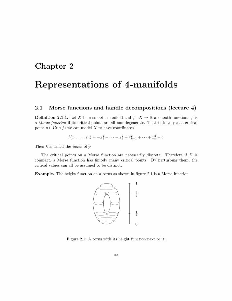
Definition 2.1.1. Let X be a smooth manifold and f : X → R a smooth function. f isa Morse function if its critical points are all non-degenerate. That is, locally at a criticalpoint p ∈ Crit(f) we can model X to have coordinates
f(x1, . . . , xn) = −x21 − · · · − x2
k + x2k+1 + · · ·+ x2
n + c.
Then k is called the index of p.
The critical points on a Morse function are necessarily discrete. Therefore if X iscompact, a Morse function has finitely many critical points. By perturbing them, thecritical values can all be assumed to be distinct.
Example. The height function on a torus as shown in figure 2.1 is a Morse function.
0
14
34
1
Figure 2.1: A torus with its height function next to it.
22
Morse functions contain topological information about a manifold in the following way:
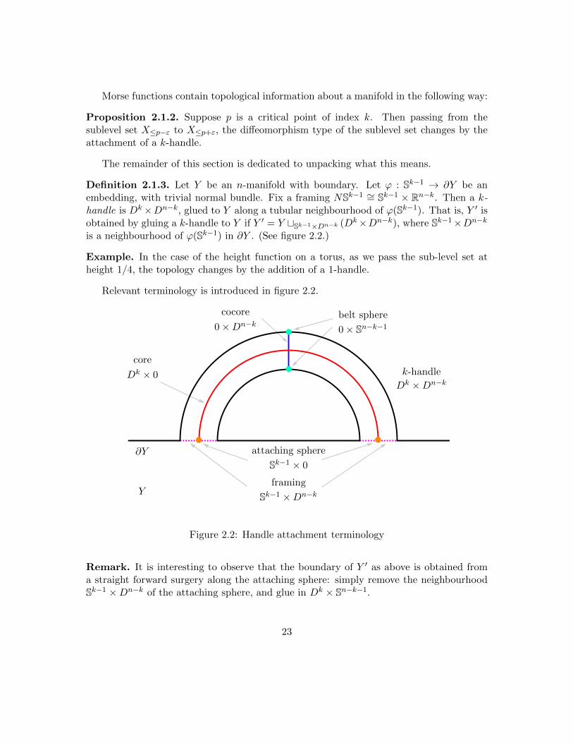
Proposition 2.1.2. Suppose p is a critical point of index k. Then passing from thesublevel set X≤p−ε to X≤p+ε, the diffeomorphism type of the sublevel set changes by theattachment of a k-handle.
The remainder of this section is dedicated to unpacking what this means.
Definition 2.1.3. Let Y be an n-manifold with boundary. Let ϕ : Sk−1 → ∂Y be anembedding, with trivial normal bundle. Fix a framing NSk−1 ∼= Sk−1 × Rn−k. Then a k-handle is Dk×Dn−k, glued to Y along a tubular neighbourhood of ϕ(Sk−1). That is, Y ′ isobtained by gluing a k-handle to Y if Y ′ = Y tSk−1×Dn−k (Dk×Dn−k), where Sk−1×Dn−k
is a neighbourhood of ϕ(Sk−1) in ∂Y . (See figure 2.2.)
Example. In the case of the height function on a torus, as we pass the sub-level set atheight 1/4, the topology changes by the addition of a 1-handle.
Relevant terminology is introduced in figure 2.2.
Y
∂Y
k-handle
Dk ×Dn−k
core
Dk × 0
cocore
0×Dn−kbelt sphere
0× Sn−k−1
attaching sphere
Sk−1 × 0
framing
Sk−1 ×Dn−k
Figure 2.2: Handle attachment terminology
Remark. It is interesting to observe that the boundary of Y ′ as above is obtained froma straight forward surgery along the attaching sphere: simply remove the neighbourhoodSk−1 ×Dn−k of the attaching sphere, and glue in Dk × Sn−k−1.
23
Proposition 2.1.4. A result from Morse theory is that every Xn admits a handle decom-position. Without loss of generality, suppose f is a Morse function on X such that thecritical points are arranged with increasing index. Then
X = X0 | X1 | · · · | Xn,
where each Xi is a union of i-handles, and the vertical line represents that Xi and Xi+1
glue together along boundary components.
Example. The torus T 2 admits a Morse function with indices 0, 1, 1, 2. Thus T 2 admitsa handle decomposition consisting of a 0-handle, two 1-handles, and a 2-handle.
Remark. The homology type of a manifold can be read off its handle decomposition!The cores of k-handles are k-cells, so Ck(X) is generated by k-handles (hkα)α∈A, with theboundary map given by
∂hkα =∑β
〈hkα, hk−1β 〉hk−1
β .
Here the angle-brackets denote the incidence number, also called the algebraic intersectionnumber. It is the signed count of intersections between attaching spheres of hkα and beltspheres of hk−1
β .
2.2 Handle moves
Theorem 2.2.1 (Cerf). Every two monotone handle decompositions of X are related bya finite sequence of handle slides and creation/cancellation of handle pairs.
By a monotone handle decomposition, we mean the manifold is decomposed into orderedlevels as in the previous proposition. We now describe the moves.
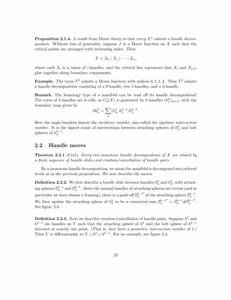
Definition 2.2.2. We first describe a handle slide between handles hkα and hkβ, with attach-
ing spheres Sk−1α and Sk−1
β . Since the normal bundles of attaching spheres are trivial (and in
particular we have chosen a framing), there is a push-off Sk−1β
′of the attaching sphere Sk−1
β .
We then update the attaching sphere of hkα to be a connected sum Sk−1α′
:= Sk−1α #Sk−1
β
′.
See figure 2.3.
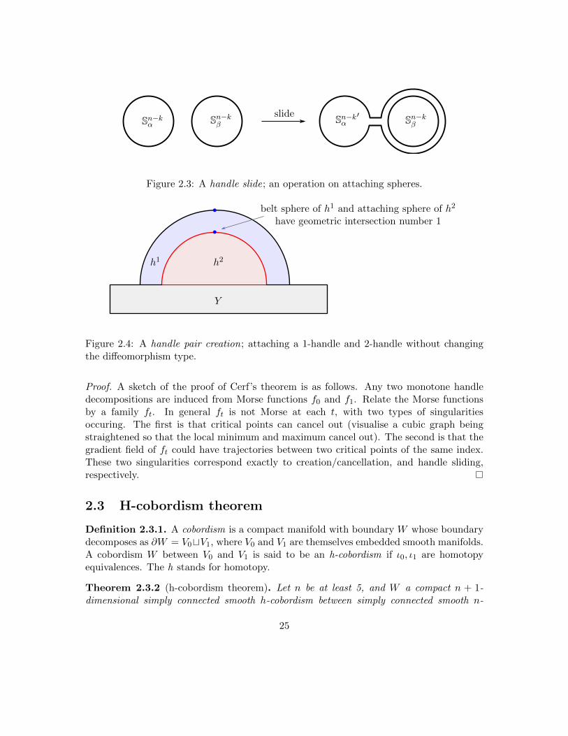
Definition 2.2.3. Next we describe creation/cancellation of handle-pairs. Suppose hk andhk−1 are handles on Y such that the attaching sphere of hk and the belt sphere of hk−1
intersect at exactly one point. (That is, they have a geometric intersection number of 1.)Then Y is diffeomorphic to Y ∪ hk ∪ hk−1. For an example, see figure 2.4.
24
Sn−kα Sn−kβSn−kβSn−kα
′slide
Figure 2.3: A handle slide; an operation on attaching spheres.
Y
h1 h2
belt sphere of h1 and attaching sphere of h2
have geometric intersection number 1
Figure 2.4: A handle pair creation; attaching a 1-handle and 2-handle without changingthe diffeomorphism type.
Proof. A sketch of the proof of Cerf’s theorem is as follows. Any two monotone handledecompositions are induced from Morse functions f0 and f1. Relate the Morse functionsby a family ft. In general ft is not Morse at each t, with two types of singularitiesoccuring. The first is that critical points can cancel out (visualise a cubic graph beingstraightened so that the local minimum and maximum cancel out). The second is that thegradient field of ft could have trajectories between two critical points of the same index.These two singularities correspond exactly to creation/cancellation, and handle sliding,respectively.
2.3 H-cobordism theorem
Definition 2.3.1. A cobordism is a compact manifold with boundary W whose boundarydecomposes as ∂W = V0tV1, where V0 and V1 are themselves embedded smooth manifolds.A cobordism W between V0 and V1 is said to be an h-cobordism if ι0, ι1 are homotopyequivalences. The h stands for homotopy.
Theorem 2.3.2 (h-cobordism theorem). Let n be at least 5, and W a compact n + 1-dimensional simply connected smooth h-cobordism between simply connected smooth n-
25
manifolds V0 and V1. Then W is diffeomorphic to V0 × [0, 1].
Proof. We now give a proof sketch of the h-cobordism theorem. We choose a Morse functionf : W → [0, 1] such that f−1(0) = V0, and f−1(1) = V1. We assume without loss ofgenerality that critical points are arranged in increasing order of index, so that W = W0 |· · · | Wn+1, where each vertical line represents a sum of cobordisms. Each Wi consists ofi-handles. The proof outline is simple:
1. Eliminate 0-handles and n+ 1-handles, so that W = W1 | · · · |Wn.
2. Eliminate 1-handles and n-handles by trading them for 3-handles and n− 2 handles,so that W = W2 | · · · |Wn−1.
3. Show that k-handles and k+ 1-handles (for 2 ≤ k ≤ n− 1) have incidence number 1.
4. Upgrade this result; show that belt spheres of k-handles and attaching spheres ofk + 1-handles (for 2 ≤ k ≤ n − 1) can be perturbed to have geometric intersectionnumber 1. Apply handle cancellation to conclude that W is a trivial cobordism.
1. Note that the attaching sphere of a 0-handle is empty. Since our handle decom-position is monotone, any 0-handle is necessarily connected with other components via1-handles. But the attaching sphere of a 1-handle consists of two points a t b, so to con-nected a 0-handle to another component, it is necessarily the case that a connects to thebelt sphere of the 0-handle, and b connects to another component. Then by handle can-cellation, the 0-handle and 1-handle cancel. This applies to n+ 1-handles, since these aredual to 0-handles by replacing f with the Morse function −f .
2. A similar procedure is used to replace 1-handles with 3-handles. Again by replacingf with −f , we trade n-handles with n− 2-handles.
3. Since W is an h-cobordism rather than just a cobordism, we can conclude thatH•(W ;V0) is trivial. Recall that C•(W ;V0) is generated by handles and is freely generatedover Z. Since the homologies vanish, up to isomorphism, the boundary maps decomposeinto a direct sum of identity maps Z→ Z. Thus the incidence numbers are 〈hkα, hk−1
β 〉 = 1.
4. We now know that the algebraic intersection numbers of belt spheres of hk−1 andattaching spheres of hk are 1. These have dimensions n− k+ 1 and k− 1. More generally,suppose P k−1 and Qn−k+1 are submanifolds of W , such that P ∩Q is contained in a levelset Zn = f−1(x). Suppose their algebraic intersection number is 1. We use the Whitneytrick to cancel intersection pairs so that their geometric intersection number is 1.
Suppose a, b ∈ P ∩Q are distinct, with opposite sign. We can find a path from a to bin Q, and a path from a to b in P . Suppose these two paths bound and embedded disk.Then by the Whitney trick we can isotope P along the disk to cancel the intersections aand b. Therefore the goal is to find and embedded disk.
First we require that the loop is homotopically trivial so that it bounds at least animmersed disk, so we want π1(Z) = 0. This comes from simple connectedness assumptions
26
in the h-cobordism theorem premises. To ensure that the disk can be embedded, we usetransversality results. We a generic perturbation of the disk to have trivial intersectionwith the disk, which happens when 2 + 2 < n. Thus we also require n ≥ 5 (as given asa premise in the h-cobordism theorem). Therefore we can make P and Q have geometricintersection number 1 as required. By applying handle cancellation, this completes theproof.
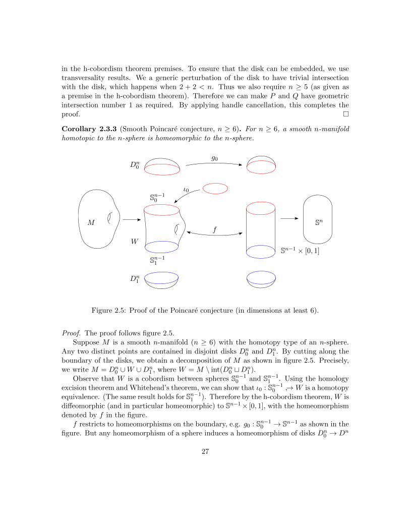
Corollary 2.3.3 (Smooth Poincare conjecture, n ≥ 6). For n ≥ 6, a smooth n-manifoldhomotopic to the n-sphere is homeomorphic to the n-sphere.
M
W
Dn0
Dn1
Sn−10
Sn−11
f
g0
Sn−1 × [0, 1]
Sn
ι0
Figure 2.5: Proof of the Poincare conjecture (in dimensions at least 6).
Proof. The proof follows figure 2.5.Suppose M is a smooth n-manifold (n ≥ 6) with the homotopy type of an n-sphere.
Any two distinct points are contained in disjoint disks Dn0 and Dn
1 . By cutting along theboundary of the disks, we obtain a decomposition of M as shown in figure 2.5. Precisely,we write M = Dn
0 ∪W ∪Dn1 , where W = M \ int(Dn
0 tDn1 ).
Observe that W is a cobordism between spheres Sn−10 and Sn−1
1 . Using the homologyexcision theorem and Whitehead’s theorem, we can show that ι0 : Sn−1
0 →W is a homotopyequivalence. (The same result holds for Sn−1
1 ). Therefore by the h-cobordism theorem, W isdiffeomorphic (and in particular homeomorphic) to Sn−1× [0, 1], with the homeomorphismdenoted by f in the figure.
f restricts to homeomorphisms on the boundary, e.g. g0 : Sn−10 → Sn−1 as shown in the
figure. But any homeomorphism of a sphere induces a homeomorphism of disks Dn0 → Dn
27
by the Alexander trick. (One can simply take the radial extension of the homeomorphism.)Therefore we have homeomorphisms g0, g1 : Dn
0 , Dn1 → Dn which agree with f on overlaps.
The map M → Dn∪ (Sn−1× [0, 1])∪Dn ∼= Sn defined piecewise by g0, f , and g is thereforea homeomorphism.
Remark. The topological Poincare conjecture is true in all dimensions. However, the h-cobordism theorem is false in dimension 4. The issue is that we cannot find embeddeddisks (only immersed) and the Whitney trick cannot be applied.
Proposition 2.3.4 (Freedman). The topological h-cobordism theorem is true in dimension4.
Freedman’s approach for proving the topological h-cobordism theorem is to removetransverse double-points in immersed Whitney disks by adding “infinite towers of handles”called Casson handles. The topological h-cobordism theorem implies the 5-dimensionaltopological Poincare conjecture. However, it also implies the 4-dimensional topologicalPoincare conjecture when combined with the following result:
Theorem 2.3.5 (Wall). Let M,N be smooth closed simply connected 4-manifolds. Supposethey have equivalent intersection forms. Then they are h-cobordant.
The proof strategy is to use the fact that the intersection forms are the same to constructa cobordism, and then use surgery to upgrade to an h-cobordism.
Corollary 2.3.6. Topological Poincare conjecture in dimension 4.
Proof. Suppose M is a 4-dimensional homotopy sphere. By Wall’s theorem, there is an h-cobordism W between M and a 4-sphere. By Freedman’s topological h-cobordism theorem,S4 × [0, 1] = W = M × [0, 1]. Therefore M is homeomorphic to S4.
Earlier it was remarked that the smooth h-cobordism theorem fails in dimension 4.However, the following result is an alternative which does hold, also due to Wall:
Theorem 2.3.7 (Wall). Let M,N be smooth closed simply connected 4-manifolds. Supposethey have equivalent intersection forms. Then M and N are stably diffeomorphic. In otherwords, there exists k ≥ 0 such that
M#k(S2 × S2) ∼= N#k(S2 × S2).
2.4 Handle decompositions of 3 and 4 manifolds (lecture 5)
Example. We first consider the case of 3-manifolds. Suppose
X3 = X0 | X1 | X2 | X3
28
where each Xi is a union of 3-dimensional i-handles. (Without loss of generality we havearranged the handles monotonically, and without loss of generality X0 and X3 are bothsingle 3-balls.) We can denote
Hg = X0 | X1, H ′g = X2 | X3,
and Σg := ∂Hg. ThenX = Hg tΣg H
′g
is called the Heegaard splitting of X. What do Hg and H ′g look like? Hg is a boundaryconnected sum of 1-handles; \g(S1 ×D2). A boundary connected sum A\B is obtained byidentifying a small disks in ∂A to one in ∂B. Thus ∂(A\B) = ∂A#∂B.
By reversing the Morse function (f 7→ −f) we see that H ′g can also be realised as
\k(S1 × D2) for some k. In fact, since H ′g and Hg have the same boundary, and k is thegenus of the boundary of H ′g, we must have that k = g. Therefore H ′g is topologically thesame as Hg!
Example. Next we consider 4-manifolds. This time we write
X4 = X0 | X1 | X2 | X3 | X4,
and again we assume X0∼= X4
∼= B4. What does X0 | X1 look like? As in the 3-manifoldcase, we have
X0 | X1∼= \k(S1 ×D3).
Similarly we know that X3 | X4 is of the same form.What about 2-handles? The attaching sphere of a 2-handle is a copy of S1. These
attaching spheres can be knotted. Precisely, the boundary of X0 | X1 is #k(S1×S2) (whichis a three manifold and hence knots and links are non-trivial), and the attaching spheresof all the 2-handles of X are given by a link L ⊂ #k(S1 × S2).
For each component S of L, we require a framing which describes the way a neighbour-hood S×D2 embeds into #k(S1×S2). (E.g. annulus vs mobius strip.) This is characterisedby the self-linking number lk(S, S) ∈ Z. (Note that the correspondence between self linkingnumber and framing depends on H1(S3) = 0.)
In summary, all 2-handles are determined by the data of a link L, where each componentis decorated with an integer.
2.5 Kirby diagrams
By the above discussion, we can represent all 2-handles by a link with each componentdecorated by an integer representing the self-linking number. On the other hand, every1-handle is determined by its attaching sphere S0. In a Kirby diagram we represent thefigure on the left (figure 2.6) by the diagram on the right: The two green spheres represent
29
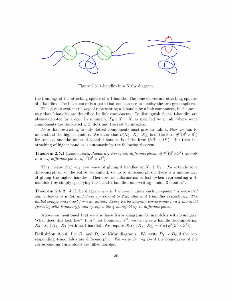
Figure 2.6: 1-handles in a Kirby diagram.
the framings of the attaching sphere of a 1-handle. The blue curves are attaching spheresof 2-handles. The black curve is a path that one can use to idenity the two green spheres.
This gives a systematic way of representing a 1-handle by a link component, in the sameway that 2-handles are described by link components. To distinguish them, 1-handles arealways denoted by a dot. In summary, X0 | X1 | X2 is specified by a link, where somecomponents are decorated with dots and the rest by integers.
Note that restricting to only dotted components must give an unlink. Now we aim tounderstand the higher handles. We know that ∂(X0 | X1 | X2) is of the form #`(S1 × S2)for some `, and the union of 3 and 4 handles is of the form \`(S1 × D3). But then theattaching of higher handles is automatic by the following theorem!
Theorem 2.5.1 (Laudenbach, Poenaru). Every self-diffeomorphism of #`(S1×S2) extendsto a self-diffeomorphism of \`(S1 ×D3).
This means that any two ways of gluing 3 handles to X0 | X1 | X2 extends to adiffeomorphism of the entire 4-manifold, so up to diffeomorphism there is a unique wayof gluing the higher handles. Therefore no information is lost (when representing a 4-manifold) by simply specifying the 1 and 2 handles, and writing “union 3 handles”.
Theorem 2.5.2. A Kirby diagram is a link diagram where each component is decoratedwith integers or a dot, and these correspond to 2 handles and 1 handles respectively. Thedotted components must form an unlink. Every Kirby diagram corresponds to a 4-manifold(possibly with boundary), and specifies the 4-manifold up to diffeomorphism.
Above we mentioned that we also have Kirby diagrams for manifolds with boundary.What does this look like? If X4 has boundary Y 3, we can give a handle decompositionX0 | X1 | X2 | X3 (with no 4 handle). We require ∂(X0 | X1 | X2) = Y#(#`(S1 × S2)).
Definition 2.5.3. Let D1 and D2 be Kirby diagrams. We write D1 ∼ D2 if the cor-responding 4-manifolds are diffeomorphic. We write D1 ∼∂ D2 if the boundaries of thecorresponding 4-manifolds are diffeomorphic.
30
Example. Consider X4 = S4. This has a handle decomposition consisting of one 0 handleand one 4 handle. Therefore it corresponds to the empty diagram.
Another handle decomposition is given by a 0 handle, 1 handle, 2 handle, and 4 handle.The corresponding diagram is then a Hopf link, with one component decorated with aninteger, and one with a dot.
Further we can dualise the decomposition, so that the sphere breaks into a 0 handle, 2handle, 3 handle, and 4 handle. Then the corresponding Kirby diagram necessarily consistsof a single unknot (union 3-handles). This is decorated with the integer 0.
Example. What is the 4 manifold corresponding to the diagram with an unknot labelledwith a non-zero integer n? This is a D2-bundle over S2, with Euler number n. It’s boundaryis the Lens space L(n, 1). Note that ∂(L(0, 1)) = S1 × S2.
Example. What about the diagram with a single dotted unknot? The correspondinghandle is S1 × D3, so it is boundary diffeomorphic to D2 × S2, which is the 2-handlerepresented by the unknot with integer 0.
Example. What about the 4-manifold represented by a single unknot, with label 1? Theboundary is L(1, 1) = S3. The corresponding manifold is in fact CP2. (One can find aMorse function on CP2 with three critical points of index 0,2, and 4.) Similarly the unknot
labelled with −1 corresponds to the manifold CP2.
Example. How about the four manifold represented by a Hopf link, both componentslabelled with 0? This is diffeomorphic to S2 × S2. This is because the height function onS2 has two critical points of index 0 and 2 respectively, so the height function on S2 × S2
has four critical points, of index 0,2,2, and 4.
Example. If D1 and D2 are Kirby diagrams for M1 and M2, their disjoint union is adiagram for M1#M2 (if the Mi are closed). If the Mi has boundary, the Kirby diagramcorresponds to the boundary connected sum.
Example. As a last example let’s look at something crazy. What does a K3 surface looklike? By Harer, Kas, and Kirby, a diagram for K3 is given in figure 2.7 (sourced fromMandelbaum: Four dimensional topology: an introduction).
We also observe that the homology of a 4-manifold can be read off the Kirby dia-gram: we know that Ck(X) is generated by k-handles, and the boundary map ∂k computesincidence numbers between k handles and k − 1 handles.
For example, if a diagram consists only of 2-handles, then Qij = lk(Li, Lj), where Liand Lj are components of the Kirby diagram. In particular, for the Hopf link with eachcomponent decorated with 0, we have Q = adiag(1, 1).
Definition 2.5.4. A Morse function f : M → R is called perfect if the number of crit-ical points is the sum of Betti numbers. Equivalently, all Morse inequalities are in factequalities.
31
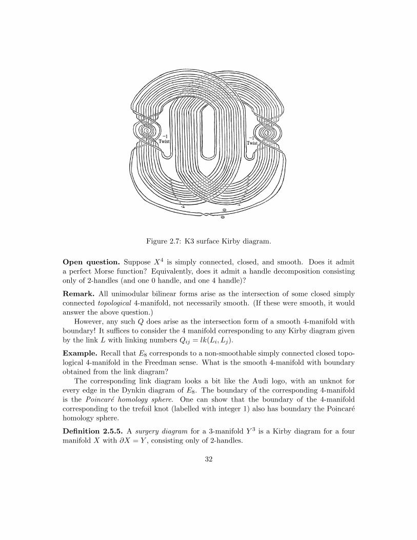
Figure 2.7: K3 surface Kirby diagram.
Open question. Suppose X4 is simply connected, closed, and smooth. Does it admita perfect Morse function? Equivalently, does it admit a handle decomposition consistingonly of 2-handles (and one 0 handle, and one 4 handle)?
Remark. All unimodular bilinear forms arise as the intersection of some closed simplyconnected topological 4-manifold, not necessarily smooth. (If these were smooth, it wouldanswer the above question.)
However, any such Q does arise as the intersection form of a smooth 4-manifold withboundary! It suffices to consider the 4 manifold corresponding to any Kirby diagram givenby the link L with linking numbers Qij = lk(Li, Lj).
Example. Recall that E8 corresponds to a non-smoothable simply connected closed topo-logical 4-manifold in the Freedman sense. What is the smooth 4-manifold with boundaryobtained from the link diagram?
The corresponding link diagram looks a bit like the Audi logo, with an unknot forevery edge in the Dynkin diagram of E8. The boundary of the corresponding 4-manifoldis the Poincare homology sphere. One can show that the boundary of the 4-manifoldcorresponding to the trefoil knot (labelled with integer 1) also has boundary the Poincarehomology sphere.
Definition 2.5.5. A surgery diagram for a 3-manifold Y 3 is a Kirby diagram for a fourmanifold X with ∂X = Y , consisting only of 2-handles.
32
Theorem 2.5.6 (Lickorish-Wallace). Every closed oriented 3-manifold admits a surgerydiagram.
2.6 Surgery diagrams (lecture 6)
Recall from the previous lecture the notion of surgery diagrams, and the Lickorish-Wallacetheorem:
Definition 2.6.1. A surgery diagram for a 3-manifold Y 3 is a Kirby diagram for a fourmanifold X with ∂X = Y , consisting only of 2-handles.
Theorem 2.6.2 (Lickorish-Wallace). Every closed oriented 3-manifold admits a surgerydiagram.
Proof. By a theorem of Rokhlin, we know that every Y 3 arises as ∂X4 for some compactsmooth manifold X. Draw a Kirby diagram for X. Since D3 × S1 is boundary isomorphicto S2×D2, we replace all 1-handles with 0-framed 2-handles to obtain a new four manifoldwhich still has boundary Y 3. By “flipping the diagram upside down”, any 3-handlescorrespond to 1-handles. By following the same procedure, we can eliminate all 3-handles.All that remains are 2-handles, as required.
Example. Some examples of surgery diagrams are as follows:
The empty diagram corresponds to S3.
The 0-framed 2-handle is S1 × S2.
An n-framed 2-handle is the lens space −L(n, 1).
The 1-framed trefoil corresponds to the Poincare sphere. The 0-framed Borromeanrings corresponds to the torus T 3.
Remark. We can read off homology from the surgery diagram! We have a Kirby diagramfor X, ∂X = Y , consisting of 2-handles. Thus H1(X) = H3(X) = 0. On the other hand,H2(X) is generated by 2-handles. This gives
H2(Y )→ H2(X)→ H2(X,Y )→ H1(Y )→ H1(X) = 0,
where the map H2(X)→ H2(X,Y ) is Q : Zr → Zr. Then H1(Y ) = cokerQ, and H2(Y ) ∼=H1(Y ) is the free part of H1(Y ).
33
2.7 Kirby calculus
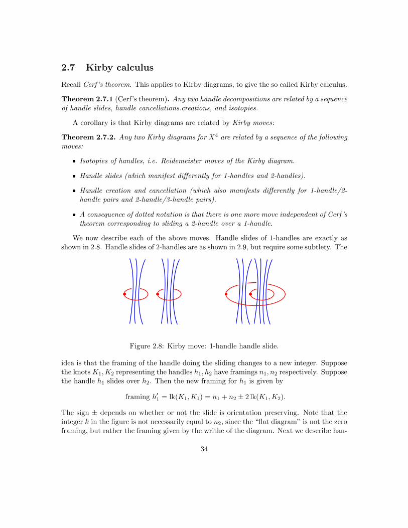
Recall Cerf’s theorem. This applies to Kirby diagrams, to give the so called Kirby calculus.
Theorem 2.7.1 (Cerf’s theorem). Any two handle decompositions are related by a sequenceof handle slides, handle cancellations.creations, and isotopies.
A corollary is that Kirby diagrams are related by Kirby moves:
Theorem 2.7.2. Any two Kirby diagrams for X4 are related by a sequence of the followingmoves:
Isotopies of handles, i.e. Reidemeister moves of the Kirby diagram.
Handle slides (which manifest differently for 1-handles and 2-handles).
Handle creation and cancellation (which also manifests differently for 1-handle/2-handle pairs and 2-handle/3-handle pairs).
A consequence of dotted notation is that there is one more move independent of Cerf ’stheorem corresponding to sliding a 2-handle over a 1-handle.
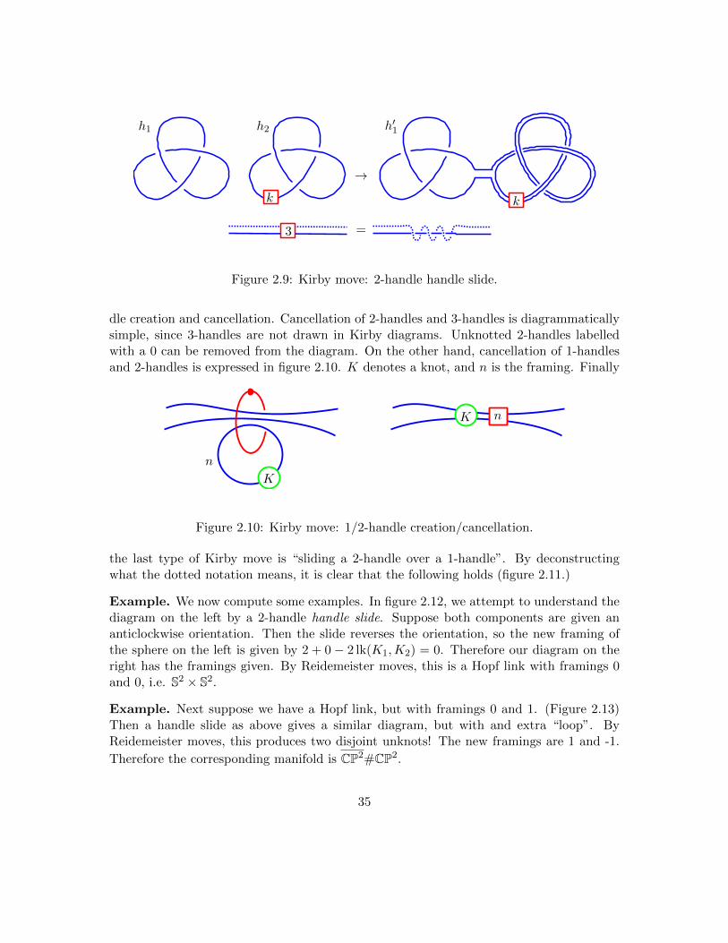
We now describe each of the above moves. Handle slides of 1-handles are exactly asshown in 2.8. Handle slides of 2-handles are as shown in 2.9, but require some subtlety. The
Figure 2.8: Kirby move: 1-handle handle slide.
idea is that the framing of the handle doing the sliding changes to a new integer. Supposethe knots K1,K2 representing the handles h1, h2 have framings n1, n2 respectively. Supposethe handle h1 slides over h2. Then the new framing for h1 is given by
framing h′1 = lk(K1,K1) = n1 + n2 ± 2 lk(K1,K2).
The sign ± depends on whether or not the slide is orientation preserving. Note that theinteger k in the figure is not necessarily equal to n2, since the “flat diagram” is not the zeroframing, but rather the framing given by the writhe of the diagram. Next we describe han-
34
→
h1 h2
k
h′1
k
3 =
Figure 2.9: Kirby move: 2-handle handle slide.
dle creation and cancellation. Cancellation of 2-handles and 3-handles is diagrammaticallysimple, since 3-handles are not drawn in Kirby diagrams. Unknotted 2-handles labelledwith a 0 can be removed from the diagram. On the other hand, cancellation of 1-handlesand 2-handles is expressed in figure 2.10. K denotes a knot, and n is the framing. Finally
K
n
K n
Figure 2.10: Kirby move: 1/2-handle creation/cancellation.
the last type of Kirby move is “sliding a 2-handle over a 1-handle”. By deconstructingwhat the dotted notation means, it is clear that the following holds (figure 2.11.)
Example. We now compute some examples. In figure 2.12, we attempt to understand thediagram on the left by a 2-handle handle slide. Suppose both components are given ananticlockwise orientation. Then the slide reverses the orientation, so the new framing ofthe sphere on the left is given by 2 + 0− 2 lk(K1,K2) = 0. Therefore our diagram on theright has the framings given. By Reidemeister moves, this is a Hopf link with framings 0and 0, i.e. S2 × S2.
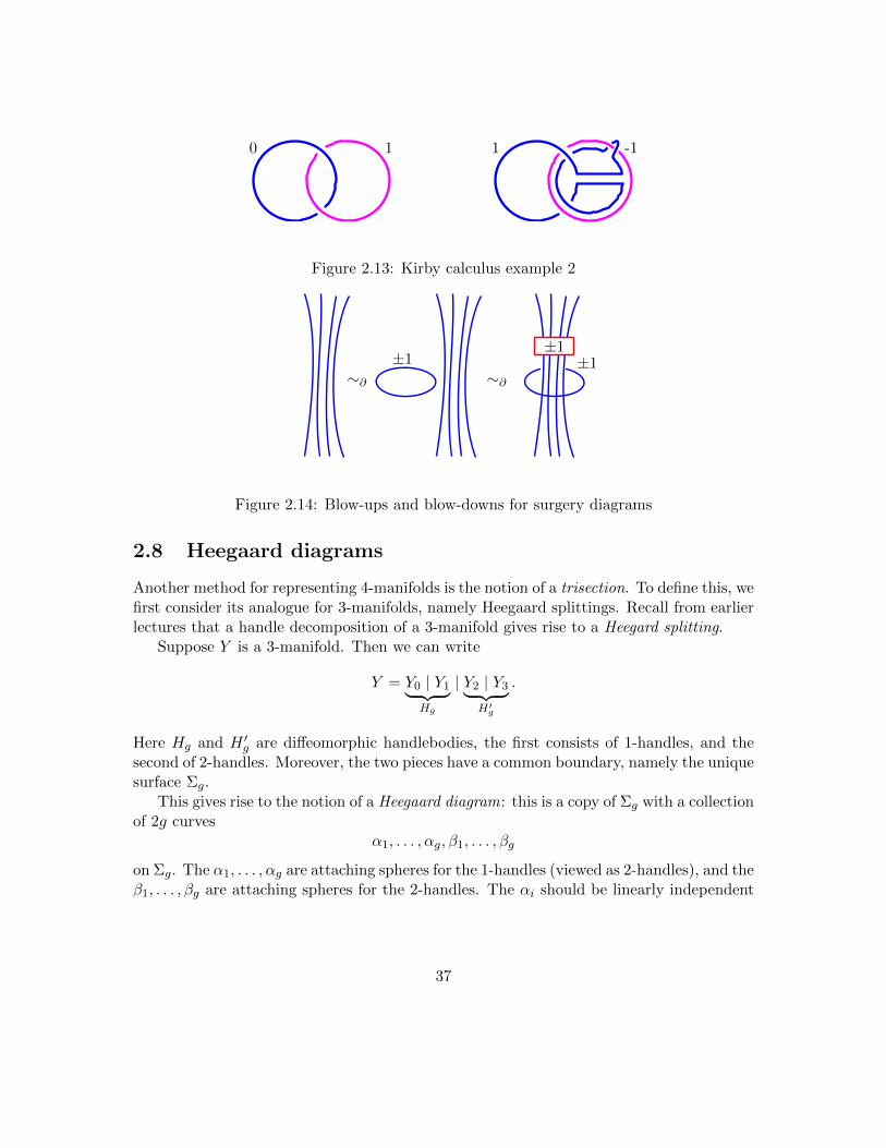
Example. Next suppose we have a Hopf link, but with framings 0 and 1. (Figure 2.13)Then a handle slide as above gives a similar diagram, but with and extra “loop”. ByReidemeister moves, this produces two disjoint unknots! The new framings are 1 and -1.
Therefore the corresponding manifold is CP2#CP2.
35

Figure 2.11: Sliding 2-handles over 1-handles.
2 0 00
Figure 2.12: Kirby calculus example
In general we find that a Hopf link with framings 0 and p represents CP2#CP2 if p isodd, and S2 × S2 is p is even.
What about the case of Hopf links with framings p, q? This gives the intersection form
Q =
(p 11 p
),
which has determinant pq − 1. This is usually not ±1! In other words, it doesn’t give avalid intersection form for a manifold without boundary. (Or with contrapositive phrasing,in general we obtain a 4-manifold with boundary.)
A similar theorem holds for surgery diagrams.
Theorem 2.7.3. Two surgery diagrams represent the same 3-manifold if and only if theyare related by Reidemeister moves, handle-slides, or blow-ups and blow-downs.
Here a blow-up or blow-down refers to the fact that ±1-framed unknots are boundaryhomeomorphic to the empty diagram. Therefore for surgery diagrams, it is completelyvalid to just drop them.
Example. Consider the Hopf-link with framing 0 and 1. Then by handle-sliding, we obtainan unlink with framing -1 and 1. By blow-downs, this corresponds to the empty diagram.Therefore the corresponding 3-manifold is S3.
Note that blow-ups and blow-downs can be generalised, as shown in figure 2.14.
36
0 1 -11
Figure 2.13: Kirby calculus example 2
∼∂ ∼∂±1
±1±1
Figure 2.14: Blow-ups and blow-downs for surgery diagrams
2.8 Heegaard diagrams
Another method for representing 4-manifolds is the notion of a trisection. To define this, wefirst consider its analogue for 3-manifolds, namely Heegaard splittings. Recall from earlierlectures that a handle decomposition of a 3-manifold gives rise to a Heegard splitting.
Suppose Y is a 3-manifold. Then we can write
Y = Y0 | Y1︸ ︷︷ ︸Hg
| Y2 | Y3︸ ︷︷ ︸H′g
.
Here Hg and H ′g are diffeomorphic handlebodies, the first consists of 1-handles, and thesecond of 2-handles. Moreover, the two pieces have a common boundary, namely the uniquesurface Σg.
This gives rise to the notion of a Heegaard diagram: this is a copy of Σg with a collectionof 2g curves
α1, . . . , αg, β1, . . . , βg
on Σg. The α1, . . . , αg are attaching spheres for the 1-handles (viewed as 2-handles), and theβ1, . . . , βg are attaching spheres for the 2-handles. The αi should be linearly independent
37
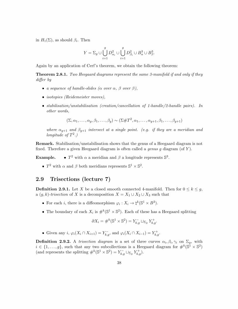
in H1(Σ), as should βi. Then
Y = Σg ∪g⋃i=1
D2αi ∪
g⋃i=1
D2βi∪B3
α ∪B3β.
Again by an application of Cerf’s theorem, we obtain the following theorem:
Theorem 2.8.1. Two Heegaard diagrams represent the same 3-manifold if and only if theydiffer by
a sequence of handle-slides (α over α, β over β),
isotopies (Reidemeister moves),
stabilisation/unstabilisation (creation/cancellation of 1-handle/2-handle pairs). Inother words,
(Σ, α1, . . . , αg, β1, . . . , βg) ∼ (Σ#T 2, α1, . . . , αg+1, β1, . . . , βg+1)
where αg+1 and βg+1 intersect at a single point. (e.g. if they are a meridian andlongitude of T 2.)
Remark. Stabilisation/unstabilisation shows that the genus of a Heegaard diagram is notfixed. Therefore a given Heegaard diagram is often called a genus g diagram (of Y ).
Example. T 2 with α a meridian and β a longitude represents S3.
T 2 with α and β both meridians represents S1 × S2.
2.9 Trisections (lecture 7)
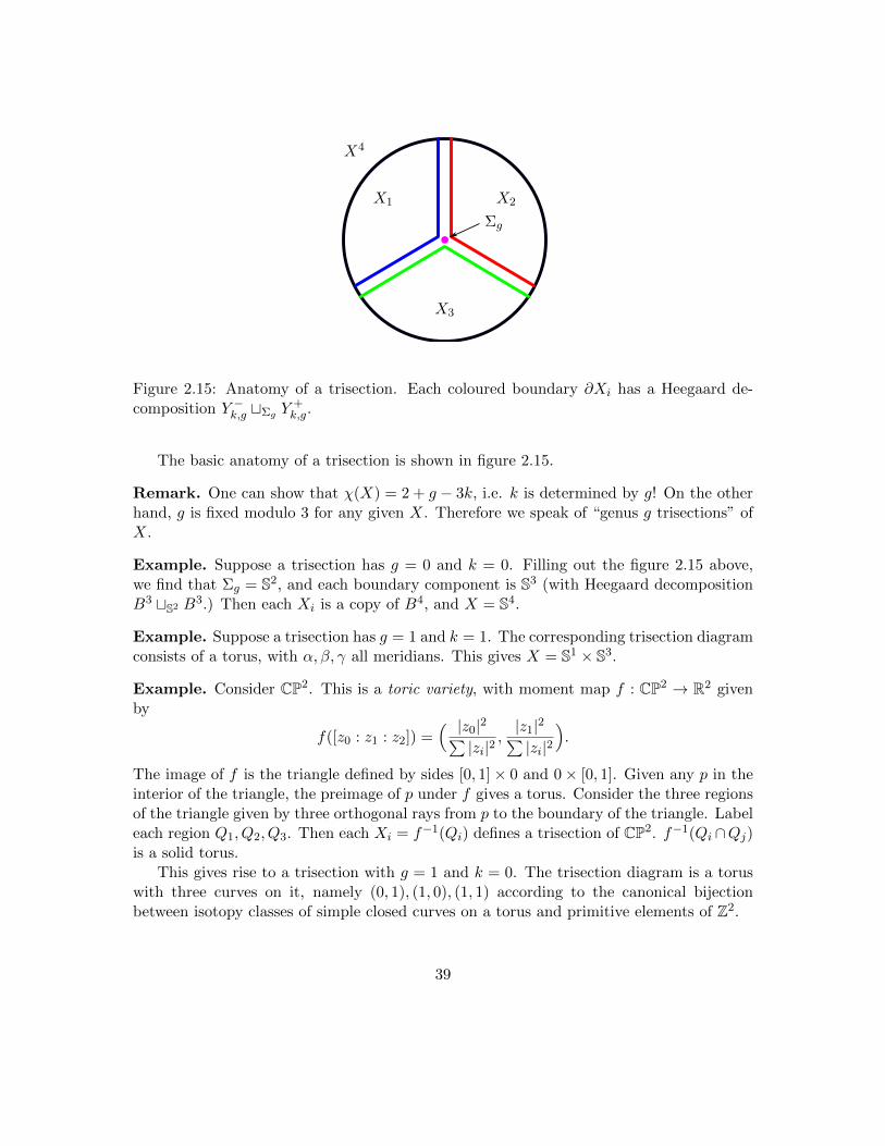
Definition 2.9.1. Let X be a closed smooth connected 4-manifold. Then for 0 ≤ k ≤ g,a (g, k)-trisection of X is a decomposition X = X1 ∪X2 ∪X3 such that
For each i, there is a diffeomorphism ϕi : Xi → \k(S1 ×B3).
The boundary of each Xi is #k(S1 × S2). Each of these has a Heegaard splitting
∂Xi = #k(S1 × S2) = Y −k,g tΣg Y+k,g.
Given any i, ϕi(Xi ∩Xi+1) = Y −k,g, and ϕi(Xi ∩Xi−1) = Y +k,g.
Definition 2.9.2. A trisection diagram is a set of three curves αi, βi, γi on Σg, withi ∈ 1, . . . , g, such that any two subcollections is a Heegaard diagram for #k(S1 × S2)(and represents the splitting #k(S1 × S2) = Y −k,g tΣg Y
+k,g).
38
X4
X1 X2
X3
Σg
Figure 2.15: Anatomy of a trisection. Each coloured boundary ∂Xi has a Heegaard de-composition Y −k,g tΣg Y
+k,g.
The basic anatomy of a trisection is shown in figure 2.15.
Remark. One can show that χ(X) = 2 + g − 3k, i.e. k is determined by g! On the otherhand, g is fixed modulo 3 for any given X. Therefore we speak of “genus g trisections” ofX.
Example. Suppose a trisection has g = 0 and k = 0. Filling out the figure 2.15 above,we find that Σg = S2, and each boundary component is S3 (with Heegaard decompositionB3 tS2 B3.) Then each Xi is a copy of B4, and X = S4.
Example. Suppose a trisection has g = 1 and k = 1. The corresponding trisection diagramconsists of a torus, with α, β, γ all meridians. This gives X = S1 × S3.
Example. Consider CP2. This is a toric variety, with moment map f : CP2 → R2 givenby
f([z0 : z1 : z2]) =( |z0|2∑|zi|2
,|z1|2∑|zi|2
).
The image of f is the triangle defined by sides [0, 1]× 0 and 0× [0, 1]. Given any p in theinterior of the triangle, the preimage of p under f gives a torus. Consider the three regionsof the triangle given by three orthogonal rays from p to the boundary of the triangle. Labeleach region Q1, Q2, Q3. Then each Xi = f−1(Qi) defines a trisection of CP2. f−1(Qi ∩Qj)is a solid torus.
This gives rise to a trisection with g = 1 and k = 0. The trisection diagram is a toruswith three curves on it, namely (0, 1), (1, 0), (1, 1) according to the canonical bijectionbetween isotopy classes of simple closed curves on a torus and primitive elements of Z2.
39
Theorem 2.9.3 (Gay-Kirby). Every closed smooth connected oriented 4-manifold admitsa trisection.
Proof. We give a proof sketch. Choose a “2-valued Morse function” f : X → B2. Thelocal models are
generic points: f is a submersion (t, x, y, z)→ (t, x)
folds: (t, x, y, z)→ (t,±x2 ± y2 ± z2)
cusps: (t, x, y, z)→ (t, x3 − tx± y2 ± z2).
We now consider a family of functions ft : X → R. Cusps occur when ft experiences thebirth or death of a singularity, and folds are curves of critical points. The image of X4
in B2 is called a Cerf graphic, and by massaging the Cerf graphic in analogous ways tohandle-moves, the Cerf graphic can be arranged to form a trisection.
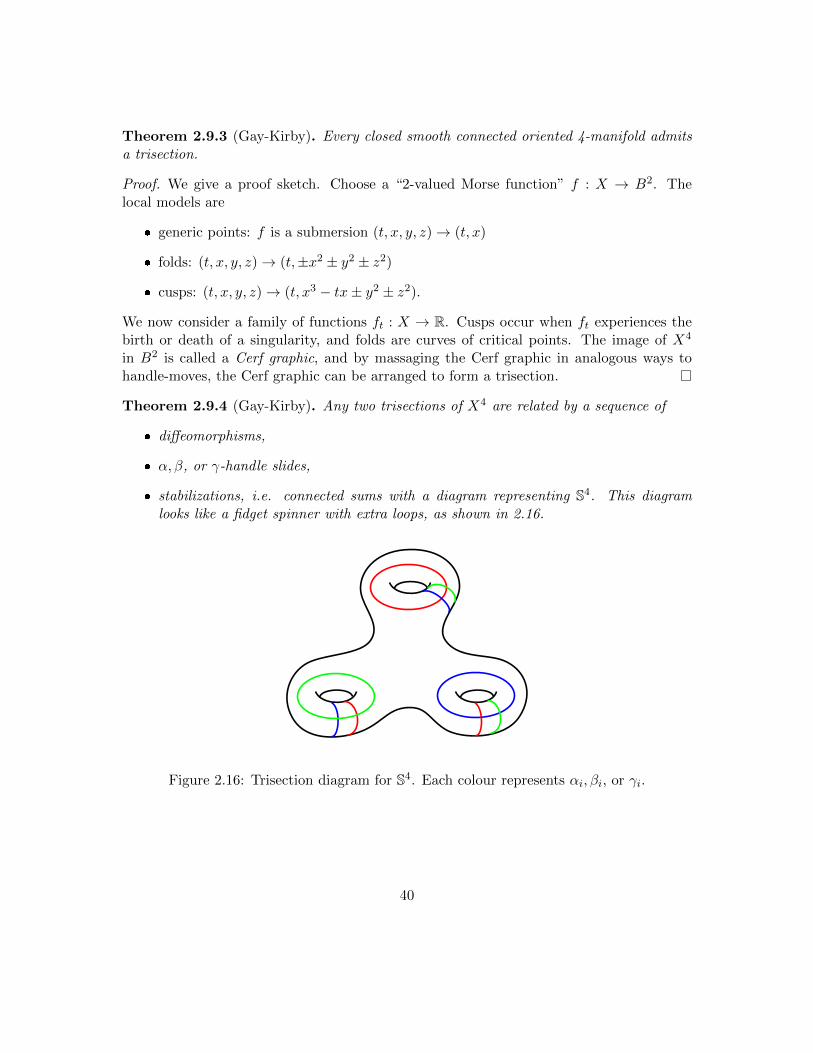
Theorem 2.9.4 (Gay-Kirby). Any two trisections of X4 are related by a sequence of
diffeomorphisms,
α, β, or γ-handle slides,
stabilizations, i.e. connected sums with a diagram representing S4. This diagramlooks like a fidget spinner with extra loops, as shown in 2.16.
Figure 2.16: Trisection diagram for S4. Each colour represents αi, βi, or γi.
40
Chapter 3
Construction of Seiberg-Wittengauge theory
Some of the goals of this section are to prove the following results:
1. Prove Donaldson’s diagonalisability theorem.
2. Show the existence of exotic smooth structures in dimension 4.
3. Prove the Thom conjecture (which concerns the genus of surfaces Σ ⊂ CP2).
4. Prove the Milnor conjecture (which concerns the genus of surfaces Σ ⊂ Tp,q).
To do this, we use the tools of Seiberg-Witten gauge theory. To state the Sieberg-Wittenequations, we must first introduce the relevant definitions.
3.1 Clifford modules
Consider the Laplacian ∆ = −∑
(∂/∂xi)2. This is an operator C∞(Rn,Cn)→ C∞(Rn,Cn).
The Laplacian is self-adjoint ; 〈∆ϕ,ψ〉 = 〈ϕ,∆ψ〉. When does the Laplacian admit a squareroot? We want
D =∑
Ai∂/∂xi, 〈Dϕ,ψ〉 = 〈ϕ,Dψ〉, D2 = ∆.
Expanding what this means, we require A2i = −1, A∗i = −Ai, and AiAj + AjAi = 0
whenever i 6= j.
Definition 3.1.1. A Clifford algebra is a real algebra generated by elements Ai satisfyingA2i = −1 and AiAj +AjAi = 0 whenever i 6= j.
41
Definition 3.1.2. Let H denote an n-dimensional real inner product space. A Cliffordmodule ofH is a Hermitian complex vector space V equipped with a Clifford multiplication,i.e. a map γ : H → End(V ) such that
1. If ‖e‖ = 1, then γ(e)2 = −1.
2. If e1 ⊥ e2, then γ(e1)γ(e2) + γ(e2)γ(e1) = 0.
3. γ(e)∗ = −γ(e).
Thus a Clifford module is a skew-Hermitian representation of a Clifford algebra.
Theorem 3.1.3. If n = 2k, then there exists a unique finite dimensional irreducible Clif-ford module (S, γ) up to isomorphism, with dimC S = 2k.
If n = 2k+1, then there are exactly two finitely dimensional irreducible Clifford modulesup to isomorphism; (S, γ) and (S,−γ). These have dimC S = 2k.
Example. Suppose H has basis e1, e2, e3. Let S = C2, and γ(ei) = Bi, where the Bi arePauli matrices:
B1 =
(i 00 −i
), B2 =
(0 ii 0
), B3 =
(0 −11 0
).
Then (S, γ) and (S,−γ) are the two Clifford modules of H, up to isomorphism.
Example. Suppose H has basis e1, e2, e3, e4. Let S = C4 = S+ ⊕ S−1, and
γ(ei) =
(0 −BiBi 0
),
where the Bi are as above, and B4 = I. Then (S, γ) is the unique irreducible module of Hup to isomorphism.
Definition 3.1.4. A spinc structure on an n-dimensional oriented Riemannian manifoldX is a Hermitian bundle S → X with bundle map ρ : TX → End(S) such that for all x,(Sx, ρx : TxX → End(Sx)) is isomorphic to an irreducible Clifford module for TxX.
Example. If n = 3, a spinc structure is a Hermitian bundle S → X of rank 2, with a mapρ : TX → End(S) such that there exists an orthonormal basis ei at each x for TxX, and aHermitian basis for S, with ρ(ei) = Bi.
In fact, this can be thought of as U(2)-bundle together with a compatibility conditionwith TX.
Example. If n = 4, a spinc structure corresponds to two Hermitian bundles S+ and S−
of rank 2, with a map ρ : TX → Hom(S+, E−), such that there is an orthonormal basis eiand Hermitian basis for S+, S−, with ρ(ei) = Bi.
Question from class. Is the category of Clifford algebras semisimple? What happens tothe earlier theorems if we drop irreducibility?
Answer. Yes, every Clifford algebra is a direct sum of irreducible Clifford algebras.
42
3.2 Spinc structure definitions (lecture 8)
Recall from the previous lecture that a spinc structure on an oriented Riemannian 4-manifold X is a pair of rank 2 Hermitian bundles S+, S− → X with bundle map ρ : TX →End(S) such that for all x, (Sx, ρx : TxX → End(Sx)) is isomorphic to an irreducibleClifford module for TxX.
More explicitly, we can refine ρ to a map γ : TX → Hom(S+, S−) ⊂ End(S). Then aspinc structure is a map γ such that for each x, there exists an orthonormal basis ei forTX and a unitary basis for S± such that
γ(ei) =
(0 −B∗iBi 0
),
where each Bi is a Pauli matrix (with B4 = I.)S = S+ ⊕ S− → X is called the spinor bundle.
Remark. Since the determinant of each Bi is 1, the determinant line bundles of S+ andS− are isomorphic. (To establish this isomorphism, it suffices to verify that ρ(e) = 1whenever ‖e‖ = 1.)
Definition 3.2.1. The class of (S, γ) is defined to be
c1(detS+) = c1(S+) = c1(S−) ∈ H2(X;Z).
Note that c1(S) = 2c1(S±).
Remark. Fix some x ∈ X. Then Aut(Sx, γx) = S1. To see this, observe that anyautomorphism commuting with γx corresponds to a pair A+ and A− of automorphismson S+ and S−, such that BiA
+ = A−Bi for each i. Since B4 = I, this implies thatA := A+ = A− ∈ U(2). On the other hand, ABiA
−1 = Bi implies that A is central, soA ∈ Z(U(2)) = S1.
Another way to think about spinc structures is via principal bundles. Recall thatSpin(n) → SO(n) is a 2:1 covering map. Then the statement that Xn is a Riemannianmanifold is equivalent to saying that the frame bundle of its tangent bundle is a principalSO(n)-bundle. A spin structure is then a lift of this structure to a Spin(n)-bundle.
With this perspective, we can define
Spinc(n) = Spin(n)×Z/2Z U(1) = (g, eiθ) ∈ Spin(n)× U(1)/ ∼
where ∼ is the equivalence relation (g, eiθ) = (τg, e−iθ). Here τg denotes the uniqueelement so that g, τg is the fibre above a point in Spin(n)→ SO(n). With this definitionof Spinc(n), a spinc structure is equivalently a lift of the frame bundle of TX to a Spinc(n)-bundle.
43
Example. Suppose n = 3. Then Spin(3) = SU(2) = S(H), where S(H) denotes the unitquaternions. There’s a 2:1 covering map
S(H)→ SO(3), h 7→ (x 7→ hxh−1).
Then Spinc(3) = SU(2) ×Z/2Z U(1) = U(2). To see this equality, for each A ∈ U(2),consider the map
A 7→ ((detA)−1/2A)((detA)1/2I).
The first component on the left belongs to SU(2), and the second to U(1). The failureof this map being well defined is that (detA)1/2 is only well defined up to sign, but thisexactly accounted for in the fibre product with respect to Z/2Z. Therefore this map givesan isomorphism, so Spinc(3) = U(2) as required. In summary we have the following result:
A spinc structure on X3 is a U(2)-bundle S → X with compatibility conditions givenby ρ : TX → End(S).
Example. Suppose n = 4. Then Spin(4) = SU(2)× SU(2)→ SO(4). The covering map isgiven by
(h1, h2) 7→ (x 7→ h1xh−12 ),
where we have again identified SU(2) with S(H). With this interpretation,
Spinc(4) = (SU(2)× SU(2))×Z/2Z U(1)
⊂ (SU(2)× 0×Z/2Z U(1))× (0× SU(2)×Z/2Z U(1)) = U(2)× U(2).
More explicitly, the subset is
Spinc(n) = (A,B) ∈ U(2)× U(2) : detA = detB ⊂ U(2)× U(2).
In summary, a four dimensional spinc structure is given by U(2)-bundles S+, S− → Xsatisfying additional compatibility conditions via γ : TX → End(S+ ⊕ S−).
3.3 Spinc structure existence and classification
Suppose X is a smooth simply connected oriented closed 4-manifold. Recall that X admitsa spin structure if and only if w2(TX) = 0, or equivalently if and only if QX is even.Existence of spinc structures is less constrained:
Proposition 3.3.1. Any smooth simply connected oriented closed 4-manifold X admits aspinc structure. The space of spinc structures is an affine space, modelled on H2(X;Z). Inother words, given any s0, s1 ∈ Spinc(X), s0−s1 is well defined in H2(X;Z). In particular,there are non-canonical isomorphisms Spinc(X) ∼= H2(X;Z).
Remark. If s ∈ Spinc(X), and h ∈ H2(X;Z) is given by h = c1(E) for a complex linebundle E, then s+ h ∈ Spinc(X) is (S+ ⊗ E,S−1 ⊗ E, ρ⊗ id).
44
Proof. We give a proof for the case where π1(X) = 1. Suppose Uαα∈A is an atlas for X,such that each Uα gives a trivialisation TX|Uα = R4 ×Uα, and Sα := S|Uα is the standardClifford module.
Choosing any α, β, we have trivialisations from each chart, with Sα corresponding toUα, and Sβ corresponding to Uβ. Thus on the intersection Uαβ, the transition map givesan isomorphism Sα → Sβ. Succinctly, we have a map
ϕαβ : Uαβ → Aut(S, γ) = S1.
Given any three charts with non-empty intersection, we can compose the above maps toobtain
ϕγα ϕβγ ϕαβ : Uαβγ → S1.
Our goal is to glue the maps over Uα to form a spinc structure on X. For this we requirethe transition maps to satisfy the cocycle condition, in this case ϕγα ϕβγ ϕαβ = 1. Whenis this true?
The obstruction to the above identity is given by Cech 2-cocycles [ϕ] ∈ H2(X,C∞S1)of the Sheaf cohomology, where
C∞S1(U) := C∞(U,S1)
for each U . We now show that this particular cohomology group vanishes. Consider thelong exact sequence
0→ Z→ C∞R exp−−→ C∞S1 → 0.
The corresponding sequence of cohomology is given by
H2(X;C∞R)→ H2(X,C∞S1)→ H3(X;Z).
The cohomology group on the left vanishes because C∞R has partitions of unity, andthe cohomology group on the right vanishes by Poincare duality (since we assumed thatπ1(X) = 0, so in particular H1(X;Z) ∼= H3(X;Z) vanishes). It follows that the cohomologygroup in the middle must also vanish, as required. This shows that our obstruction vanishes,completing the proof of existence in the case π1(X) = 0.
For the general case, it turns out that even if π1(X) doesn’t vanish (so that H3(X;Z)is non-trivial), we can still look at the image of H2(X,C∞S1) under the induced map toconclude that the cohomology group is trivial.
Question from class. Doesn’t this imply spin structures exist?
Answer. No, recall that spin structures exist if and only if QX is even. The reason wedon’t have a contradiction here is because there is no map Spinc → Spin (because of the“modulo 2”). We only have a natural map Spinc → SO, which is perfectly fine since thelatter is a Riemannian structure.
45
Proposition 3.3.2. Classification: suppose (S, γ) and (S′, γ′) are two spinc structures.On Uα, we obtain isomorphisms ψα : (S, γ)|Uα → (S′, γ′)|Uα , and on an intersection Uαβ,we have ψα ψ−1
β : Uαβ → Aut(S, γ) = S1. This gives a 1-cocyle in H1(X;C∞S1). But
this cohomology group is in fact isomorphic to H2(X;Z), from the exact sequence
0 = H1(X;C∞R)→ H1(X;C∞S1)→ H2(X;Z)→ H2(X;C∞R) = 0.
Therefore spinc structures exist, and are non-canonically isomorphic to H2(X;Z) (they areaffine over H2(X;Z)).
Remark. The above result depends on dimension 4: there exist 6-dimensional manifoldsadmitting no spinc structures.
Recall that we defined the class of a spinc structure (S, γ) to be the first Chern classc1(S±) = c1(detS±). For h ∈ H2(X;Z), we noted that s+ h ∈ Spinc(X) was given by thebundle S± ⊗ E, where E is a complex line bundle with c1(E) = h. Therefore if c denotesthe class of s, then the class of s+ h is given by
c1(S+ ⊗ E) = c1(detS+ ⊗ E2) = c1(S+) + 2c1(E) = c+ 2h.
If H2(X;Z) has no 2-torsion, (e.g. π1(X) = 0), then s ∈ Spinc(X) is determined by itsclass, c1(s) = c1(S+). In other words, the map c1 : Spinc(X)→ H2(X;Z) is an injection.
What is the image of c1 : Spinc(X)→ H2(X;Z)? One can show that these are exactlythe characteristic elements of X;
im c1 = k ∈ H2(X;Z) : k mod 2 = w2(TX) = char(X).
Note that k mod 2 = w2(TX) means that 〈k, a〉 = 〈a, a〉 modulo 2.For example, if X is spin, then w2(TX) vanishes. Therefore Spinc(X) is isomorphic
to the characteristic elements of X, which are 2H2(X;Z) ⊂ H2(X;Z). If X = CP2, thenH2(X;Z) = Z and QX = (1). The characteristic elements of CP2 are 2Z + 1 ⊂ Z.
3.4 Hodge theory
Let V denote an inner product space over R, equipped with an orientation. That is, achoice of volume form vol ∈ ΛnV . The Hodge star is the map
? : ΛkV → Λn−kV
such that α ∧ ?β = 〈α, β〉vol. Explicitly, if I = i1, . . . , ik ⊂ 1, . . . , n, then vI =ei1 ∧ · · · ∧ eik gives a basis for ΛkV , and ?vI = ±vI , where I is the complement of I in1, . . . , n.
46
Example. When k = 2, and the dimension of V is 4, then
dim Λ2V =
(4
2
)= 6,
with? : Λ2V → Λ2V, ?2 = 1, Λ2V = Λ+V ⊕ Λ−V
where Λ±V are the ± eigenspaces of ?. What are the bases for the eigenspaces? For Λ+V ,we have basis
e1 ∧ e2 + e3 ∧ e4, e1 ∧ e3 − e2 ∧ e4, e1 ∧ e4 + e2 ∧ e3.
For Λ−V , we have a basis
e1 ∧ e2 − e3 ∧ e4, e1 ∧ e3 + e2 ∧ e4, e1 ∧ e4 − e2 ∧ e3.
Suppose X is an oriented Riemannian 4-manifold. Then
Λ2T ∗X = Λ+T ∗X ⊕ Λ−T ∗X.
The first factor on the right consists of self-dual 2-forms, and the second factor, anti-self-dual 2-forms.
Definition 3.4.1. H2(X;R) denotes the harmonic 2-forms,
H2(X;R) = ω ∈ Ω2(X) : dω = d?ω = 0.
Here d? = − ? d?. The action of ? on harmonic 2-forms gives a decomposition
H2(X;R) = H+ ⊕H−
of ± eigenspaces. The self-dual forms give a cohomology theory with H = H+.
3.5 Hodge meets spinc (lecture 9)
Recall that the Hodge star is a map
? : Ωk(M)→ Ωn−k(M),
where M is a closed oriented n-manifold. On the other hand, the exterior derivative is amap
d : Ωk(M)→ Ωk+1(M),
which gives rise to the de Rham complex, with cohomology Hk(M ;R) = ker d/ im d. Wealso define the dual of the exterior derivative by
d? = ± ? d? : Ωk+1(M)→ Ωk(M).
47
Theorem 3.5.1. The Hodge decomposition theorem states that
Ωk(M) = im d⊕Hk(M)⊕ im d?,
where Hk(M) = ω ∈ Ωk(M) : ∆ω = 0 are the Harmonic 2-forms, and ∆ = dd? + d?d.
Now suppose X is a 4-manifold, so ? : Ω2(X)→ Ω2(X) is an involution (?2 = 1). Then
Ω2(X) = Ω2+(X)⊕ Ω2
−(X),
where Ω2±(X) are the ± eigenspaces of ?. We can further define projection operators
Π± : Ω2(X)→ Ω2±(X) by
Π± =1± ?
2,
so that Π+ + Π− = 1. We can further define a complex (analogously to the de Rhamcomplex),
Ω0(X)d−→ Ω1(X)
d+
−−→ Ω2+(X), d+ = Π+ d.
Then the second cohomology H2+ of the above complex is exactly the + eigenspace of ?
acting on H2(X).How does the Hodge star interact with spinc structures? Suppose X is a 4-manifold
with spinc structure (S, γ). More explicitly, γ : TX → Hom(S, S), with
γ(ei) =
(0 −B∗iBi 0
),
so the γ(ei) anticommute. X is Riemannian, so we have a (musical) isomorphism TX ∼=T ∗X. Combining these two observations, γ extends to maps
ΛkTX ⊗ C→ End(S), γ(ei1 ∧ · · · ∧ eik) = γ(ei1) · · · γ(eik).
Lemma 3.5.2. Λ2+ ⊂ Λ2TX acts trivially on S−, and γ : Λ2
+ → su(S+) is an isomorphism.Note that
su(S+) = A ∈ End(S+) : A∗ = −A, tr(A) = 0.
Proof. Check in local bases. For example, e1 ∧ e2 + e3 ∧ e4 acts trivially on S− sinceB1(−B∗2) +B3(−B∗4) = 0.
Corollary 3.5.3. Fix ω ∈ Ω2+(X). This gives a section γ(ω) ∈ Γ(su(S)).
48
3.6 Connections and curvature
Definition 3.6.1. An “E-valued k-form” is an element of
Ωk(X;E) = Γ(ΛkT ∗X ⊗ E),
where E → X is a vector bundle. In particular, Ω0(X;E) = Γ(E).
Definition 3.6.2. Let X be a smooth manifold, and E → X a vector bundle. A connection∇A on E is an operator
∇A : Ω0(X;E)→ Ω1(X;E)
satisfying the Leibniz rule, i.e.
∇A(fs) = df ⊗ s+ f∇As
for all smooth f : X → R and s ∈ Γ(E).
Remark. If ∇A and ∇B are connections, then
(∇A −∇B)(fs) = f(∇A −∇B)(s).
Therefore the difference of connections is not a connection, but rather it belongs to Γ(Hom(E, T ∗X⊗E)) = Ω1(X; End(E)). Hence the set connections on E is an affine space over Ω1(X; End(E)).
Definition 3.6.3. Now let E be a Hermitian complex vector bundle. A connection ∇Aon E is unitary if
d〈s, t〉 = 〈∇As, t〉+ 〈s,∇At〉
for all s, t ∈ Γ(E).
Remark. If ∇A and ∇B are unitary connections, then their difference ∇ = ∇A − ∇Bsatisfies
〈∇s, t〉+ 〈s,∇t〉 = 0,
so ∇ ∈ Ω1(X; u(E)) where u(E) is the unitary Lie algebra, and can be viewed as a subsetof End(E). Hence the set unitary connections on E is an affine space over Ω1(X; u(E)).
Definition 3.6.4. Let X4 be a manifold with spinc structure (S, γ). A spinc connection∇A on S is a unitary connection such that
∇A(γ(v)s) = γ(v)∇As+ γ(∇LCv)s
for all v ∈ Γ(TX), s ∈ Γ(S). On the left side, γ(v)s is Clifford multiplication, and ∇LC isthe Levi-Civita connection.
49
Remark. If ∇A,∇B are spinc connections, then ∇ = ∇A −∇B satisfies
∇(γ(v)s) = γ(v)∇s.
Therefore the set spinc connections on S is an affine space over Ω1(X; End(S, γ)∩u(S))On one hand, End(S, γ) consists of diagonal matrices zI, and on the other, u(S) forcesz∗ = −z. Therefore we can make the identification
Ω1(X; End(S, γ) ∩ u(S)) = Ω1(X; iR).
Hence spinc connections on S is an affine space over Ω1(X; iR).
Definition 3.6.5. The curvature of a connection ∇A is simply given by FA = ∇A ∇A.
The idea is that ∇A induces a connection on higher exterior powers, so the above isreally a composition of maps
Γ(E)→ Γ(T ∗X ⊗ E)→ Γ(Λ2T ∗X ⊗ E).
Then for any f : X → R and s ∈ Γ(E), we have
FA(fs) = ∇A(df ⊗ s+ f∇As) = d2f ⊗ s+ df ⊗∇As− df ⊗∇As+ fFAs = fFAs.
This shows that FA ∈ Ω2(X; End(E)).
Remark. The curvature measures the failure of exactness of the “E-valued de Rhamcomplex”.
The curvature satisfies the following properties:
Let ∇A have curvature FA. Then there is a canonical connection ∇Aτ on det(E),with curvature FAτ = tr(FA).
c1(E) =[
12πFAτ
]∈ im(H2(X;Z)→ H2(X;R)).
Suppose X is a spinc 4-manifold, with ∇A a spinc connection, FA ∈ Ω2(X; iR). In thiscase, FA = 1
2FAτ . Further define F+A = Π+ FA ∈ Ω2
+(X; iR) ∼= Γ(su(S+)).For any Φ ∈ Γ(S), we obtain an element (iΦΦ∗)0 ∈ Γ(su(S+)). The idea is that
h = iΦΦ∗ ∈ Γ(S ⊗ S∗) = Γ(End(S)) is map
h : ψ 7→ iΦ〈Φ, ψ〉,
so that h∗ = −h. To ensure that h lies in Γ(su(S+)), we take the trace free part,
h0 = h− 1
2(trh)I.
50
With this in mind, we define
σ(Φ) = γ−1(ΦΦ∗)0 ∈ Ω2+(X; iR).
In fact, we’ve now developed enough terminology and machinery to state one of the Seiberg-Witten equations:
F+A = σ(Φ).
Definition 3.6.6. Let X4 be a 4-manifold with spinc structure (S, γ) and spinc connection∇A. The Dirac operator is defined by the composition
Γ(S)∇A−−→ Γ(T ∗X ⊗ S)
g−→ Γ(TX ⊗ S)γ−→ Γ(S).
This is denoted by DA (or sometimes DA or ∂A). In fact, we can write
DA =
(0 D−AD+A 0
), D+
A : Γ(S+)→ Γ(S−).
Example. Suppose X denotes Euclidean 4-space, with S+ = S− = C2 the trivial bundle.A spinc structure is given by
γ(ei) =
(0 −B∗iBi 0
)= Ai.
Then a spinc connection is given by the the exterior derivative by identifying C2 to withR4. Therefore the Dirac operator is given by
s∇A7−−→ ds
g7−−→∑i
ei∂s
∂xiγ7−−→(∑
i
Ai∂
∂xi
)s.
Therefore
DA =∑i
Ai∂
∂xi.
But this is exactly a square root of the Laplacian! Recall that the Ai satisfies A2i = −1,
and AiAj +AjAi = 0 for i 6= j.
Example. Suppose (X4, g, (S, γ),∇A) are arbitrary. Then DA isn’t necessarily a squareroot of the Laplacian - it will also have some curvature terms. Explicitly, this is given bythe Weitzenbock formula:
D2AΦ = ∇∗A∇AΦ +
s
4Φ +
1
2γ(FA)Φ.
In the above, s denotes the scalar curvature of (X, g). The first term on the right is theLaplacian for Spinors; ∇∗A∇A. The second term is a curvature term from g, and the thirdterm is the curvature from ∇A.
51
Question from class. Does the above formulation hold in pseudo-Riemannian settings?
Answer. Yes, the formulas above come from universal polynomial equations.
Question from class. Do connections always exist?
Answer. Yes, you can locally trivialise the relevant bundles and locally define the trivialconnection. Then by using partitions of unity, the local structures can be glued together.
3.7 Seiberg-Witten equations
Definition 3.7.1. Let X be a spinc 4-manifold, with spinc connection ∇A. Then theSeiberg-Witten equations are
D+AΦ = 0, F+
A = σ(Φ)
where Φ is a positive spinor, i.e. Φ ∈ Γ(S+), where S = S+ ⊕ S− → X and γ : TX →End(S) gives the spinc structure. Recall that σ is a “squaring map”, σ(Φ) = γ−1((ΦΦ∗)0).
What are some properties of the Seiberg-Witten equations? A very important propertyis Gauge invariance. Let G = Γ(Aut(S, γ)) = C∞(X,S1). This is called the Gauge group.For any u ∈ G, u · Φ ∈ Γ(S+), and we can define u · ∇A to be
u · ∇A = ∇A − u−1du.
This comes from the Leibniz rule, by computing u(∇A(u−1Φ)). Note that du ∈ Ω1(X; iR),so if u = ef with f : X → iR, then u−1du = df .
Proposition 3.7.2. The Seiberg-Witten equations are gauge invariant. That is, for anyu ∈ G, if ∇A and Φ satisfy the Seiberg-Witten equations, so do u · ∇A and u · Φ.
This is a non-trivial result in the sense that G is very large! It is an infinite dimensionalgroup.
Definition 3.7.3. Let ∇A0 be a fixed spinc connection. We say that A is in Coulombgauge with respect to A0 if d?(A−A0) = 0.
Everything can be put in Coulomb gauge by applying some u ∈ G. In particular,solutions to the Seiberg-Witten equations modulo G are equivalent to solutions to Seiberg-Witten in the Coulomb gauge modulo H1(X;Z)× S1.
52
3.8 Seiberg-Witten moduli space (lecture 10)
We consider X a closed smooth oriented Riemannian 4-manifold with metric g, and spinc
structure s = (S, γ) ∈ Spinc(X), S = S+ ⊕ S−. For simplicity, for the remainder of thislecture we assume X is simply connected (π1(X) = 0).
Recall the Seiberg-Witten equations:
D+AΦ = 0, F+
A = γ−1((ΦΦ∗)0),
for A a spinc connection, and Φ ∈ Γ(S+). The Gauge group is G = Γ(Aut(S, γ)) =C∞(X,S1). Then the Seiberg Witten moduli space is
MSW = (A,Φ) satisfying SW/G = (A,Φ) satisfying SW in Coulomb gauge/S1.
Recall that a spinc connection A is in Coulomb gauge with respect to A0 if d?(A−A0) = 0.Our goal is to count solutions to the Seiberg-Witten equations. To make sure this is welldefined, we begin by proving that MSW is compact.
Theorem 3.8.1. MSW is compact.
Proof. Suppose (A,Φ) is a solution to SW. By Weitzenbock,
D2AΦ = ∇∗A∇AΦ +
s
4Φ +
1
2γ(FA)Φ.
On the other hand,
d〈Φ,Φ〉 = 〈∇AΦ,Φ〉+ 〈Φ,∇AΦ〉 = 2Re〈∇AΦ,Φ〉.
It follows that
1
2∆|Φ|2 =
1
2d?d〈Φ,Φ〉 = d?(Re〈∇AΦ,Φ〉) ≤ 〈∇∗A∇AΦ,Φ〉.
But now by applying the Weitzenbock formula, we have
∇∗A∇AΦ,Φ〉 = 〈D2AΦ,Φ〉 − s
4〈Φ,Φ〉 − 1
2〈γ(FA)Φ,Φ〉.
Since (A,Φ) solves SW, D2AΦ = 0, so the first term on the right vanishes. Moreover,
γ(F+A ) = γ(γ−1(ΦΦ∗)0).
Since Ω2− acts trivially on S+, γ(FA)Φ = (ΦΦ∗)0Φ. In summary we have
〈∇∗A∇AΦ,Φ〉 = −s4|Φ|2 − 1
2〈(ΦΦ∗)0Φ,Φ〉.
53
In a unitary basis at some x ∈ X we can write Φ = (t, 0), where t = |Φ|. Then
ΦΦ∗ =
(|t|2 00 0
), so that (ΦΦ∗)0 =
1
2
(|t|2 00 −|t|2
).
But then 〈(ΦΦ∗)0Φ,Φ〉 = 12 |Φ|
4. Overall, this gives
1
2∆|Φ|2 ≤ 〈∇∗A∇AΦ,Φ〉 ≤ −s
4|Φ|2 − 1
4|Φ|4.
Since X is compact, we can choose x ∈ X which maximises |Φ|. Then 0 ≤ ∆|Φ|2, so eitherΦ = 0 or |Φ|2 ≤ −s. In particular, if s ≥ 0, then Φ = 0. These pointwise bounds on Φ giveLp bounds on Φ. This induces bounds on F+
A = γ−1((ΦΦ∗)0).Write A = A0 + ia, where a ∈ Ω1(X;R). Then F+
A = F+A0
+ id+a. By the Coulombcondition, we have −id?(A−A0) = d?a = 0. Now considering the homology of
Ω0 d−→ Ω1 d+
−−→ Ω+2 ,
we have H1(X;R) = a : d+a = d?a = 0. It follows that
d+ + d? : Ω1 → Ω+2 ⊕ (Ω0/R)
is a linear elliptic injective Fredholm operator. This provides an elliptic estimate. Namely, abound on (d++d?)a induces a bound on a in some Sobolev norm. By elliptic bootstrapping,this gives C∞ bounds on a and Φ, which then gives compactness.
3.9 Counting solutions to SW
Solutions to the Seiberg-Witten equations are classified in the following two ways:Reducible, Φ = 0 fixed points of S1 action.
Irreducible, Φ 6= 0 S1 action is free: eiθ : (A,Φ) 7→ (A, eiθΦ).
We first investigate reducible solutions. These satisfy the following properties:
Φ = 0, DAΦ = 0, F+A = 0, F+
A0+ d+a = 0,
where a = A − A0. Therefore we have an injective map d+ + d? on the collection of asatisfying d?a = 0 and d+a = −F+
A0. We conclude that there is either one solution or no
solutions satisfying these properties.
Proposition 3.9.1. The Seiberg-Witten equations have 0 or 1 reducible solutions.
54
Our next goal is to count irreducible solutions. Define
SW : Connections⊕ Γ(S+)→ Ω2+(X; iR)⊕ Γ(S−)⊕ (Ω0(X)/R)
by(∇A,Φ) 7→ (F+
A − γ−1((ΦΦ∗)0), D+
AΦ, d?(A−A0)).
We claim that MSW = SW−1
(0)/S1. (Again we are assuming for simplicity that our fourmanifold is simply connected.) For this to be true, we require that 0 is a regular value, sothat the preimage is really a submanifold. Therefore we compute the derivative:
dSW (A,Φ) = (d+ + 〈Φ, . . .〉, D+A0
+ · · · , d?).
This is a linear elliptic Fredholm operator! Therefore the index defined by
ind(dSW ) = dim ker dSW − dim coker dSW ∈ Z.
This is invariant under deformations. By the famous Aityah-Singer index theorem, we canactually compute this:
ind(dSW ) =c1(s)2 − σ(X)
4− b+2 (X) + b1(X).
(In our case, b1(X) = 0.) Here σ(X) is the signature of the intersection form on X. Sincethe index is invariant under deformations, we consider perturbed Seiberg-Witten equations:
SW (A,Φ) = (η, 0, 0), η ∈ Ω2+(X; iR).
Then SW−1
(η, 0, 0) is still compact, and we define MSW ,η
= SW−1
(η, 0, 0)/S1. By the
transversality theorem, for generic η, SW−1
(η, 0, 0) is a smooth manifold of dimension the
index of dSW . In summary we have established the following:
Proposition 3.9.2. For generic η, SW−1
(η, 0, 0) is a smooth manifold of dimension
ind(dSW ).
To conclude that the quotient SW−1
(η, 0, 0)/S1 is a smooth manifold, we want the S1
action to be free. But in general the action isn’t quite free, since reducible solutions tothe Seiberg-Witten equations might exist. We now determine some conditions to eliminateany reducible solutions. Recall that a reducible solution satisfies
SW (A,Φ) = (η, 0, 0), Φ = 0, F+A = F+
A0+ d+a = η, d?a = 0.
Inspecting the sequence
Ω0 → Ω1 d+
−−→ Ω2+,
55
we find that reducible solutions exist if and only if η−F+A0
lies in the image of d+. This is
a codimension b2+(X) condition, so to guarantee that there are no reducible solutions forgeneric η, it suffices to assume that b2+(X) > 0.
Finally recall that the signature and Euler characteristic of a 4-manifold is given by
σ(X) = b+2 − b−2 , χ(X) = 2− 2b1 + b+2 + b−2 .
Proposition 3.9.3. If b2+(X) > 0, then for generic η,
MSW,η =MSW (X, s, g, η) = SW−1
(0)/S1
is a smooth compact manifold of dimension
d =c1(s)2 − σ(X)
4− b+2 + b1 − 1 =
c1(s)2 − (3σ(X) + 2χ(X))
4.
In particular, when d = 0, MSW,η is a finite collection of points.
3.10 The Seiberg-Witten invariant
In summary we have shown that “counting solutions” is well defined, given a perturbationand b2+(X) > 0.
Definition 3.10.1. The Seiberg-Witten invariant SWX(s, g, η) of X is the signed count ofpoints inMSW,η, for some fixed choice of orientations. More precisely, we fix a “homologyorientation”, i.e. we orient H0(X)⊕H1(X)⊕H2
+(X).
Remark. The above definition implicitly assumes that d = 0. However, the definition canbe extended to any even d > 0. But in all known cases, it turns out that SWX = 0 forpositive d.
Remark. A 4-manifold X is of simple type if SWX(s) = 0 for all s with d > 0. Witten’sconjecture is that all 4-manifolds are of simple type. This is known to be true for symplectic4-manifolds (e.g. all complex projective surfaces).
Theorem 3.10.2. If b+2 (X) ≥ 2, then SWX(s, g, η) is independent of generic η and g.
Proof. Consider (g0, η0), (g1, η1) in metrics×Ω2+. We interpolate by a family (gt, ηt). Then
M =⋃t∈[0,1]MSW,(gt,ηt) is a smooth manifold of dimension d + 1 = 1. We can avoid
reducibles in a one-parameter family: to do this, we require b+2 ≥ 2, since existence ofreducibles are a codimension b+2 condition as mentioned earlier. Now M is a 1-manifoldwith boundary −MSW,(g0,η0) tMSW,(g1,η1). But the signed count of boundary points ofany 1-manifold is always zero!
56
Hereafter we write SWX(s), for s ∈ Spinc(X), given the assumption b+2 ≥ 2 and d = 0.
Remark. When b+2 = 1, there is a wall of perturbations in which reducibles exist. Thiswall partitions the space metrics×Ω2
+ into two chambers. We denote the chambers by ±,and the Seiberg-Witten invariant takes two values SW+
X (s) and SW−X (s), which differ by±1.
Recall that Spinc(X) is an affine space over H2(X;Z). When π1(X) = 1, we have aninjective map
c1 : Spinc(X)→ H2(X;Z).
The image consists of characteristic elements:
Spinc(X) ∼= k ∈ H2(X;Z) : 〈k, a〉 = 〈a, a〉 mod 2 for all a = Char(X).
With this identification established, we can give the final juicy definition of the Seiberg-Witten invariant:
Definition 3.10.3. The Seiberg-Witten invariant of a four manifold X is the map
SWX : Char(X)→ Z
defined by SWX(k) = SWX(s) for a Spinc structure s satisfying c1(s) = k.
We explore the properties of the Seiberg-Witten invariant in the following lecture, andlook at some applications.
57
Chapter 4
Applications of Seiberg-Wittentheory
4.1 Basic properties of SW (lecture 11)
Recall that the Seiberg-Witten invariant was defined as a map
SWX : Char(X)→ Z.
We will see that SWX(k) often vanishes.
Definition 4.1.1. A characteristic element k ∈ Char(X) is called a basic class if SWX(k) 6=0.
Eight basic properties of the Seiberg-Witten invariant are as follows:
1. SWX(k) = 0 for all but finitely many k. In other words, there are only finitely manybasic classes.
2. If X admits a metric of positive scalar curvature, then SWX vanishes identically.
3. The Seiberg-Witten invariant satisfies a notion of symmetry:
SWX(−k) = (−1)b+2 (X)−b1(X)+1SWX(k).
(In our case we only established the existence of the Seiberg-Witten invariant for sim-ply connected 4-manifolds so that b1(X) = 0. However, the Seiberg-Witten invariantsexist more generally, in which case the above formula is the correct generalisation.)
4. Another important vanishing property of the Seiberg-Witten invariant is the follow-ing: suppose X = X1#X2, where b+2 (Xi) ≥ 1 for both i ∈ 1, 2. Then SWX
identically vanishes.
58
5. A related property is called the blow up formula. Suppose X is of simple type, withbasic classes k1, . . . , ks. Then
X ′ = X#CP2
has basic classes ki ± E : i = 1, . . . , s, where E ∈ H2(CP 2;Z). (This is called the
exceptional class, and represents CP1 in CP2.) Moreover,
SWX′(ki ± E) = ±SWX(ki).
6. So far we have only shown that SW vanishes in various cases, but have yet to exhibitthat SW is ever non-trivial. This is remedied here.
Suppose X is a complex projective surface. Then ±c1(TX) are characteristic ele-ments, and
SWX(±c1(TX)) = ±1.
7. The following is a generalisation of the previous property, due to Taubes: let X besymplectic, and J a compatible almost-complex structure. Then
SWX(±c1(TX, J)) = ±1.
8. Adjunction inequality.
(a) Let Σ ⊂ X be an embedded oriented closed surface, with self intersection number[Σ]2 at least 0, and [Σ] 6= 0. Then for any basic class k on X,
2g(Σ)− 2 ≥ [Σ]2 + |k · [Σ]|
(where k · [Σ] is again the intersection number).
(b) If X is of simple type, and g(Σ) 6= 0, the above result also holds in the casewhere [Σ]2 < 0.
4.2 Basic applications of SW
Using these properties, one huge result we can prove is the existence of exotic structureson four manifolds.
Example. Define the following 4-manifolds:
X1 = K3#CP2, X2 = (#3CP2)#(#20CP2).
Then X1 and X2 are connected sums of simply connected manifolds, and hence simplyconnected. Hence by Freedman’s theorem, if X1 and X2 have equivalent intersection forms,they are homeomorphic. Explicitly, we have
QX1 = 2(−E8)⊕ 3
(0 11 0
)⊕ (−1), QX2 = 3(1)⊕ 20(−1).
59
One way of seeing these are equivalent is to use the classification of unimodular bilinear
forms. Specifically, we see that QX1 = 2(−E8) ⊕ 3
(0 11 0
)⊕ (−1) is indefinite and odd.
Therefore it is equivalent to m(1)⊕ n(−1) for unique m,n. By inspection, we see that
m+ n = 2× 8 + 3× 2 + 1 = 23, m− n = 2× (−8) + 0− 1 = −17.
Therefore m = 3 and n = 20, so QX1 is equivalent to QX2 . It follows that X1 and X2 arehomeomorphic.
To see that they are not diffeomorphic, we show that they have different Seiberg-Witten invariants. Since a K3 surface is a complex projective variety, by property 6,SWK3(c1(TK3)) = ±1. But we also know that K3 surfaces are Calabi-Yau, so in particularc1(TK3) = 0. (One way to see this is to recall that Zd ⊂ CP3 can be defined as the zeroset of a homogeneous degree d polynomial in 4 variables, and then c1(TZd) = (4− d)h forsome h. In particular, K3 = Z4, giving us the desired result. This calculation was givenin the section on characteristic classes earlier in the notes.)
Therefore SWK3(0) = ±1. Next by property 5 (the blow up formula), the exceptional
class E ∈ H2(CP2;Z) satisfiesSWX1(E) = ±1.
On the other hand, we can write
X2 = (#2CP2)#(CP2#(#20CP2).
This expresses X2 as a connected sum of two 4-manifolds each with b+2 ≥ 1. Therefore byproperty 4, SWX2 identically vanishes. In particular, SWX1 6= SWX2 , so X1 and X2 arenon-diffeomorphic smooth manifolds.
Finally we note that the vanishing result can also be proven geometrically, using prop-erty 2. By a theorem of Schoen and Yau, if M1,M2 are manifolds of dimension n at least3, and M1 and M2 each admit metrics with positive scalar curvature, then so does the con-
nected sum. Therefore by noting that the Fubini-Study metric on CP2,CP2 has positivecurvature, we conclude that X2 admits a metric of positive scalar curvature as required.Thus SWX2 = 0.
Example. Next consider X1 = Z5 ⊂ CP3. This is a “surface of general type”, obtainedas the zero set of a quintic homogeneous polynomial in four variables. We also consider
X2 = (#9CP2)#(#44CP2). Both X1 and X2 can be shown to be simply connected, with
QX1 = 9(1)⊕ 44(−1) = QX2 .
Therefore by Freedman’s theorem, they are homeomorphic. By property 6, X1 has non-trivial Seiberg-Witten invariant, but X2 has everywhere vanishing Seiberg-Witten invariantby property 2 or 4. Therefore X1 and X2 are not diffeomorphic.
60
Other applications are the following theorems:
Theorem 4.2.1. Let X be a symplectic simply connected closed 4-manifold. Then thereis no decomposition X = X1#X2, such that b+2 (Xi) > 0 for both i ∈ 1, 2.
Proof. Suppose X has a decomposition X = X1#X2, such that b+2 (Xi) > 0 for bothi ∈ 1, 2. Then SWX vanishes identically by property 4. However, If X is symplectic,property 7 ensures that SWX does not vanish everywhere. Therefore X cannot have adecomposition as above.
Theorem 4.2.2. There exist simply connected almost-complex 4-manifolds that are notsymplectic.
Proof. Recall that an almost complex structure onX is a complex structure J ∈ End(TX), J2 =−1 on TX. That is, (TX, J) is a complex bundle over X.
By algebraic topology, if X is a simply connected 4-manifold, it admits an almostcomplex structure if and only if b+2 (X) is odd. But now we can take X = #3CP2, andthis is almost complex since b+2 = 3. However, it cannot be symplectic by the previoustheorem, since
X = (CP2)#(#2CP2),
and then both factors have positive b+2 . Therefore by the previous theorem, X cannot besymplectic.
Question from class. So far all of the SW invariants seem to be 0 or 1, do we ever getlarge numbers?
Answer. Yes, we can get 200, or 300, or, well, any integer you want!
4.3 Proofs of the basic properties
Property 1, finiteness. There are only finitely many basic classes. This follows from com-pactness of the moduli space.
Property 2, curvature. SW vanishes identically on any 4-manifold admitting a metric withpositive scalar curvature. This follows from the Weitzenbock formula.
Property 3, symmetry. SWX(−k) = (−1)b+2 (X)−b2(X)+1SWX(−k). Let (S, γ : TX →
End(S)) be a spinc structure. This has a conjugate structure, (S∗, γ∗), where S∗ ∼= Svia the Hermitian metric. Then c1(S+) = −c1(S+). Finally the result follows from theone-to-one correspondence
Solutions of SW for (S, γ) ↔ Solutions of SW for (S∗, γ∗).
61
Property 4, connected sum. If X = X1#X2, with b+2 (Xi) ≥ 1, then SWX = 0. For ourproof outline, we assume X is of simple type. X1#X2 can be decomposed as X1 and X2
glued together with a cylinder S3 × [−T, T ] between them. The process of neck stretchingsends T to ∞. Then studying the limit, we can show that
MSW (X) ∼= MSW (X1)× MSW (X2),
where MSW (X) consists of (A,Φ) satisfying the Seiberg-Witten equations, and d?(A0 −A) = 0 for some A0. Thus MSW = MSW /S1.
But now taking their products, the additional factor of S1 manifests in that MSW (X)is an S1-bundle over MSW (X1)×MSW (X2). Here the fibre of S1 corresponds to a gluingparameter. Less formally, we have
Solutions to SW on X ↔ solutions on X1, solutions on X2, gluing parameter.
But now if d(X, s) denotes the “expected dimension of MSW ”, namely
c1(s)2 − σ4
− b+2 + b1 − 1,
then we must have0 = d(X, s) = d(X1, s1) + d(X2, s2) + 1.
Therefore one of d(Xi, si) must be negative, so there are no irreducible solutions for suchand (Xi, si). Hence SWX = 0.
Property 5, blow-up formula. If X ′ = X#CP2, and X is of simple type, the basic classesof X ′ are exactly k ± E where k is a basic class of X, and E is the exceptional class of
CP2. Since b+2 (CP2) = 0, reducible solutions exist generically. Therefore we obtain exactly
one reducible solution on (CP2,±E), even though d(CP2,±E) = −1. Pairing this withirreducibles on (X, s) gives irreducibles on (X#CP 2, s± E).
Property 6, non-triviality. SWX is non-trivial on complex projective surfaces. The idea isto interpret solutions to SW on complex surfaces as divisors. Then s = c1(TX) correspondsto the empty curve, from which we conclude that SWX(±c1(TX)) = ±1.
Property 7, non-triviality 2. If X is symplectic and J is a compatible almost complex struc-ture, then SWX(±c1(TX, J)) = ±1. This is a huge result proven by Taubes using hardanalysis. The result is called “SW = GW”, in which it was shown that the Gromov-Witten invariants and Seiberg-Witten invariants are equal (when they are both defined).While SW counts solutions to the SW equations, GW counts the number of J-holomorphiccurves.
62
Property 8, adjunction inequality, part (a). Let Σ ⊂ X be embedded oriented closed, withnon-negative self-intersection number. Then 2g(Σ)− 2 ≥ [Σ]2 + |k · [Σ]| for any basic classk.
The first step in this proof is to reduce the inequality to a slightly easier one. Byproperty 3 (symmetry), we can replace k with −k, so that it suffices to prove k · [Σ]+[Σ]2 ≤2g(Σ)− 2 without the absolute value.
The second step in this proof (which is all we can prove in the remainder of thislecture) is to reduce to the case where [Σ]2 = 0. We do this via the blow up formula:
suppose X = X#CP2. Then this contains Σ = Σ#CP1 as an embedded oriented closedsurface of the same genus as Σ. Moreover, k is basic in X if and only if k − E is basic inX. Computing intersection numbers, we have
[Σ]2 = [Σ]2 + [CP1]2 = [Σ]2 − 1.
This gives a way of reducing intersection numbers. Next to verify that the reduction isvalid, we need to ensure that the adjunction formula holds for Σ if it holds for Σ. This isindeed the case:
2g(Σ) ≥ [Σ]2 + (k − E) · [E]
⇒ 2g(Σ)− 2 ≥ [Σ]2 − 1 + k · [E]− E[CP1] = [Σ]2k · [E].
Therefore we can inductively blow up until the self intersection number is zero. We nowproceed with the main proof.
Claim: If [Σ]2 = 0, then k · [Σ] ≤ 2g(Σ) − 2. Since [Σ]2 = 0, it has a neighbourhooddiffeomorphic to Σ × D2 ⊂ X. Recalling the result from the previous lecture concerningmetric independence (for generic metrics), whenever SWX(k) 6= 0, it must be the case thatMSW (X, s, g) 6= 0 for all metrics g. This is because being non-zero is an open condition.Therefore there exists a solution (A,Φ) to the Seiberg-Witten equations on X for anymetric g, with no perturbation.
Which metric will we choose? We again do some neck-stretching: we can write X as
(D2 × Σ) ∪ ([0, R]× S1 × Σ) ∪ (X − (D2 × Σ)).
For each R, will consider g on X to restrict to the product metric on the cylinder [0, R]×S1 × Σ. On the first two factors the metric is canonical, and on Σ we choose g to be theconstant curvature metric with volume equal to 1. (Typically Σ is hyperbolic, but mayalso be a torus or a sphere.) We will study how (A,Φ) behaves as R goes to infinity. Thisproof is continued in the following lecture.
4.4 Proof of the adjunction inequality for SW (lecture 12)
In the previous lecture, we started a proof of the adjunction inequality, which is one ofthe properties of the Seiberg-Witten invariant. Here we complete the proof. First let us
63
restate the result.
Proposition 4.4.1. Let X be a smooth 4-manifold with b+2 ≥ 2. Let Σ ⊂ X be a smoothlyembedded oriented connected surface. Assume [Σ]2 ≥ 0, with [Σ] 6= 0. Then for any basicclass k,
2g(Σ)− 2 ≥ [Σ]2 + |k · [Σ]|.
Moreover, if X is of simple type, and g(Σ) 6= 0, this result holds for all Σ.
The second part of the theorem is due to Ozsvath and Szabo, and we do not give aproof. For the first part, we continue the proof from where we left in the previous lecture.
Proof. In the previous lecture, we showed that we can reduce the problem to showing that
2g(Σ)− 2 ≥ k · [Σ]
in the case where [Σ]2 = 0. In this setting, we will consider metrics on X and study somebounds on solutions to the SW equations.
Lemma 4.4.2. Let (A,Φ) be a solution to the Seiberg-Witten equations on X. Then if sdenotes the scalar curvature of X,
2√
2‖F+A ‖ ≤ ‖s‖
where ‖ · ‖ is the L2 norm on X.
Proof. We use some bounds established in earlier lectures using the Weitzenbock formula.In particular, we established that
〈∇∗A∇AΦ,Φ〉 = −s4|Φ|2 − 1
4|Φ|4.
Integrating each term of X, we have∫|∇AΦ|2 +
1
4
∫|Φ|4 =
1
4
∫(−s)|Φ|2.
Applying the Cauchy-Schwarz inequality to the right hand side gives
1
4
∫(−s)|Φ|2 ≤ 1
4
(∫s2)1/2(∫
|Φ|4)1/2
.
Combining this with the above equation, we have
1
4
∫|Φ|4 ≤
∫|∇AΦ|2 +
1
4
∫|Φ|4 ≤ 1
4
(∫s2)1/2(∫
|Φ|4)1/2
.
64
If Φ vanishes identically the desired inequality holds trivially. Otherwise we divide throughby (
∫|Φ|2)1/2/4 to obtain
‖|Φ|2‖ =(∫|Φ|4
)1/2≤(∫
s2)1/2
≤ ‖s‖.
Since F+A = γ−1((ΦΦ∗)0), writing Φ = (t, 0), we can compute (as in an earlier lecture) that
|Φ| = t, while
(ΦΦ∗)0 =1
2
(t2 00 −t2
).
But now |(ΦΦ∗)0| = 12 t
2. Next we note that γ changes this norm by a factor of square-root-2, so |F+
A | = |γ−1(ΦΦ∗)0| = 12√
2t2 = |Φ|2. These pointwise equalities give an L2
equality,
8‖F+A ‖
2 = 8
∫|F+A |
2 =
∫|Φ|4 = ‖|Φ|2‖.
Taking the root of each side and equating with the previous inequality gives
2√
2‖F+A ‖ ≤ ‖s‖
as desired.
Our goal is to establish the adjunction inequality by combining this result with theGauss-Bonnet theorem. Before we do this we need one more lemma:
Lemma 4.4.3. Let α ∈ Ω2(X4) be closed. Then [α]2 = ‖α+‖2 − ‖α−‖2 (where the normsare again in L2).
Proof. This is a direct calculation:
[α]2 =
∫Xα ∧ α
=
∫(α+ + α−) ∧ (α+ + α−)
=
∫α+ ∧ α+ +
∫α− ∧ α− + 2
∫α− ∧ α+
=
∫α+ ∧ ?α+ −
∫α− ∧ ?α− − 2
∫α+ ∧ ?α−
= ‖α+‖2 − ‖α−‖2 + 2〈α+, α−〉 = ‖α+‖2 − ‖α−‖2.
65
We now apply the two previous lemmas to bound ‖FA‖. From Chern-Weil theory, wecan write
c1(S+) = [i
2πFA].
Therefore by the most recent lemma,
0 = ‖F+A ‖
2 − ‖F−A ‖2 − 4π2c1(S+)2.
On the other hand, we also have ‖FA‖2 = ‖F+A ‖2 + ‖F−A ‖2. Adding the two expressions
gives
‖FA‖2 = 2‖F+A ‖
2 − 4π2c1(S+)2
≤ 1
4‖s‖2 + constant.
We now restrict ourselves to a certain family of metrics to control the scalar curvatureterm. We write
X = (D2 × Σ) ∪ ([0, R]× Σ× S1) ∪ (X −D2 × Σ).
where the “cylinder” is embedded between the two pieces on the ends. We choose metricsgR which restrict to the product metric on the cylinder, and are the constant-curvaturemetric with volume 1 on Σ. We will later consider the limit as R goes to infinity, which iscalled neck stretching. We write X = C ∪ (X − C).
Since gR is fixed on the non-cylinder parts of X, we have∫s2 =
∫X−C
s2 +
∫Cs2 = constant +R
∫Σs2
Σ.
By the Gauss-Bonnet theorem, since we chose our metric to be the volume-one constantcurvature metric on Σ, we have∫
Σκ = 2π(2g − 2) ⇒ sΣ = 2κ = 4π(2g − 2).
Combining this with the previous inequality, we obtain an almost-topological bound on‖FA‖, namely
‖FA‖2 ≤ R(2π(2g − 2))2constant.
From Chern-Weil theory, the left side is in fact a bound for k · [Σ]. That is, for any R,
R(2π〈c1(S+), [Σ]〉)2 = R(∫
ΣFA
)2≤∫C|FA|2 ≤
∫X|FA|2 = ‖FA‖2.
Therefore for any R, we have
R(2π〈c1(S+), [Σ]〉)2 ≤ R(2π(2g − 2))2constant
where the constant is independent of R. It follows that
k · [Σ] = 〈c1(S+), [Σ]〉 ≤ 2g − 2
as required.
66
4.5 Resolving the Thom conjecture using SW
The Thom conjecture is a lower bound on the genus of a smoothly embedded projectivesurface representing an algebraic curve. To establish these bounds, we pair the adjunctioninequality with the adjunction formula (which we now state).
Theorem 4.5.1. Let X4 be equipped with an almost complex structure J . Suppose Σ ⊂ Xis J-holomorphic, with J∗(TΣ) = TΣ. Then
2g(Σ)− 2 = [Σ]2 − c1(TX, J) · [Σ].
Proof. We decompose the tangent bundle as
TX|Σ = TΣ⊕NΣ.
Thenc1(TX) · [Σ] = c1(TΣ) · [Σ] + c1(NΣ) · [Σ] = χ(Σ) + [Σ]2.
For example, this formula applies to complex curves in complex projective surfaces, orJ-holomorphic curves in symplectic 4-manifolds.
Theorem 4.5.2 (Symplectic Thom conjecture, Osvath-Szabo 1998). Let (X,ω) be a sym-plectic 4-manifold, and Σ ⊂ X a symplectic surface with volume form ω|Σ. Then Σ isgenus minimising in its homology class.
By genus minimising, we mean any other embedded surface representing the samehomology class (not necessarily symplectic) has genus at least that of Σ.
Proof. We note that [ω]2 = [ω∧ω] > 0, so b+2 (X) ≥ 1. We give a proof assuming b+2 (X) ≥ 2,and describe how to prove the general case later.
If Σ = S2, the result holds trivially. Therefore we assume Σ has positive genus, andb+2 (X) ≥ 2. Since X is symplectic, it is of simple type. By a result of Taubes, since Xis symplectic, k = −c1(TX) is a basic class. Choose J compatible with ω such that Σ isJ-holomorphic.
Let S ⊂ X be any other surface with [S] = [Σ]. Then
2g(S)− 2 ≥ [S]2 + k · [S] = [Σ]2 + k · [Σ] = 2(Σ)− 2,
where the first equality uses the adjunction inequality, and the second uses the adjunctionformula. It follows that g(S) ≥ g(Σ), so Σ is genus minimising.
If b+2 (X) = 1 (which is the remaining case), then SW takes values which change by ±1passing between each of the two chambers. By carefully working through the details, thesame proof holds.
67
Theorem 4.5.3 (Thom conjecture, Kronheimer-Mrowka 1994). Let S ⊂ CP2 be a smoothlyembedded surface, representing the homology class [C] of a degree d complex projective curveC. Then
g(S) ≥ (d− 1)(d− 2)
2= g(C).
Proof. First by the symplectic Thom conjecture, g(S) ≥ g(C). It remains to show that(d−1)(d−2)
2 = g(C). This follows from the adjunction formula:
2g(C)− 2 = [C]2 + k · [C] = d2 − 3d.
Therefore g(C) = (d− 1)(d− 2)/2.
Corollary 4.5.4 (Local Thom conjecture). Let Σ ⊂ C2 be an affine algebraic smoothcurve. Then Σ is locally genus minimising.
By locally genus minimising, we mean that if B ⊂ C2 is a ball, ∂B t Σ, and S ⊂ B isa surface such that ∂S = S ∩ ∂B = Σ ∩ ∂B, then
g(S|B) ≥ g(Σ|B).
Proof. This follows from the Thom conjecture. Compactify Σ to obtain Σ. Perturb toensure smoothness. Similarly perturb S so that S∩∂B = Σ∩∂B. By the Thom conjecture,
g(S ∪ (Σ−B)) ≥ g(Σ).
It follows that g(S|B) ≥ g(Σ|B) = g(Σ|B) as required.
4.6 Resolving the Milnor conjecture using SW
The Milnor conjecture concerns the value of the slice genus of torus knots. Notions of knotgenus are generally hard to compute since they consider minimums over large families ofobjects. Nevertheless, the slice genus of a torus knot can be computed using the localThom conjecture.
Definition 4.6.1. Let K ⊂ S3 be a knot. The slice genus of K is
gs(K) = ming(S) : S ⊂ B4, ∂S = S ∩ ∂B = K.
Definition 4.6.2. A slice knot is a knot with slice genus 0. In other words, any knot thatbounds a smoothly embedded disk in the four-ball.
Corollary 4.6.3. If K arises as a transverse intersection ∂B∩S, with S an affine algebraiccurve, then gs(K) = g(S|B).
68
Proof. This is immediate from the local Thom conjecture.
Corollary 4.6.4 (Milnor conjecture, Kronheimer-Mrowka 1993). Let Tp,q denote the p, q-torus knot. Then
gs(Tp,q) =(p− 1)(q − 1)
2.
Proof. By the previous corollary, it remains to show that the torus knot Tp,q arises asthe intersection of an affine algebraic curve Σ and ∂B4, where the genus of Σ ∩ B is(p− 1)(q − 1)/2.
Let p, q ≥ 1, with gcd(p, q) = 1. Then wrapping p strands on a torus longitudinally,with q twists around the meridian, we obtain the torus knot Tp,q. Consider the surface
Σ = xp − yq = 0 ⊂ C2.
Then it can be shown that Tp,q = Σ ∩ ∂B(√
2) as follows: first observe that ∂B(√
2) =|x|2 + |y|2 = 2 contains the torus T 2 = |x| = 1 × |y| × 1. Then the parametrisationx = eiqθ, y = eipθ realises the knot, for θ ∈ [0, 2π].
Unfortunately, our Σ is not quite smooth! We therefore deform to Σε = xp − yq − ε.This is now smooth, and Σε ∩ ∂B(
√2) is isotopic to Σ ∩ ∂B(
√2).
Next we determine the genus of Σε ∩ B(√
2). Consider the projection map (x, y) ∈Σε 7→ x ∈ C. This is a q : 1 covering map, branched over the points with xp = ε. Tocompute the genus of Σε, we can therefore use the Riemann-Hurwitz formula:
1− 2g(Σε ∩B) = χ(Σε ∩B) = qχ(D2)− p(q − 1) = p+ q − pq.
Therefore
g(Σε ∩B) =(p− 1)(q − 1)
2
as required.
In the next lecture, we will see how this generalises to quasi-positive knots.
4.7 Knots bounding affine algebraic curves (lecture 13)
We continue studying some of the implications of Seiberg-Witten theory on knots. One ofthe “goals” of knot theory is to determine unknotting numbers - this is the most intuitiveinvariant measuring the complexity of a knot, but is in general difficult to determine.
Definition 4.7.1. Let K be a knot. The unknotting number of K, denoted u(K), isthe minimum number of crossing changes required to turn K into the unknot, where theminimum is taken over all diagrams.
69
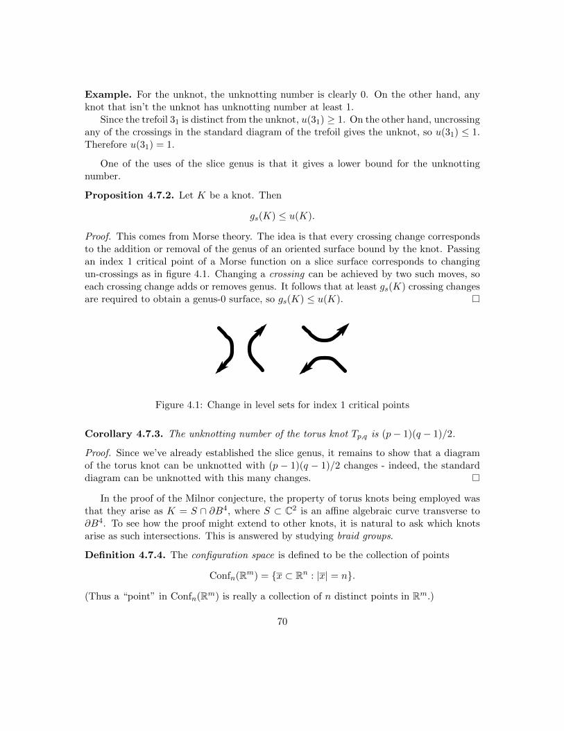
Example. For the unknot, the unknotting number is clearly 0. On the other hand, anyknot that isn’t the unknot has unknotting number at least 1.
Since the trefoil 31 is distinct from the unknot, u(31) ≥ 1. On the other hand, uncrossingany of the crossings in the standard diagram of the trefoil gives the unknot, so u(31) ≤ 1.Therefore u(31) = 1.
One of the uses of the slice genus is that it gives a lower bound for the unknottingnumber.
Proposition 4.7.2. Let K be a knot. Then
gs(K) ≤ u(K).
Proof. This comes from Morse theory. The idea is that every crossing change correspondsto the addition or removal of the genus of an oriented surface bound by the knot. Passingan index 1 critical point of a Morse function on a slice surface corresponds to changingun-crossings as in figure 4.1. Changing a crossing can be achieved by two such moves, soeach crossing change adds or removes genus. It follows that at least gs(K) crossing changesare required to obtain a genus-0 surface, so gs(K) ≤ u(K).
Figure 4.1: Change in level sets for index 1 critical points
Corollary 4.7.3. The unknotting number of the torus knot Tp,q is (p− 1)(q − 1)/2.
Proof. Since we’ve already established the slice genus, it remains to show that a diagramof the torus knot can be unknotted with (p − 1)(q − 1)/2 changes - indeed, the standarddiagram can be unknotted with this many changes.
In the proof of the Milnor conjecture, the property of torus knots being employed wasthat they arise as K = S ∩ ∂B4, where S ⊂ C2 is an affine algebraic curve transverse to∂B4. To see how the proof might extend to other knots, it is natural to ask which knotsarise as such intersections. This is answered by studying braid groups.
Definition 4.7.4. The configuration space is defined to be the collection of points
Confn(Rm) = x ⊂ Rn : |x| = n.
(Thus a “point” in Confn(Rm) is really a collection of n distinct points in Rm.)
70
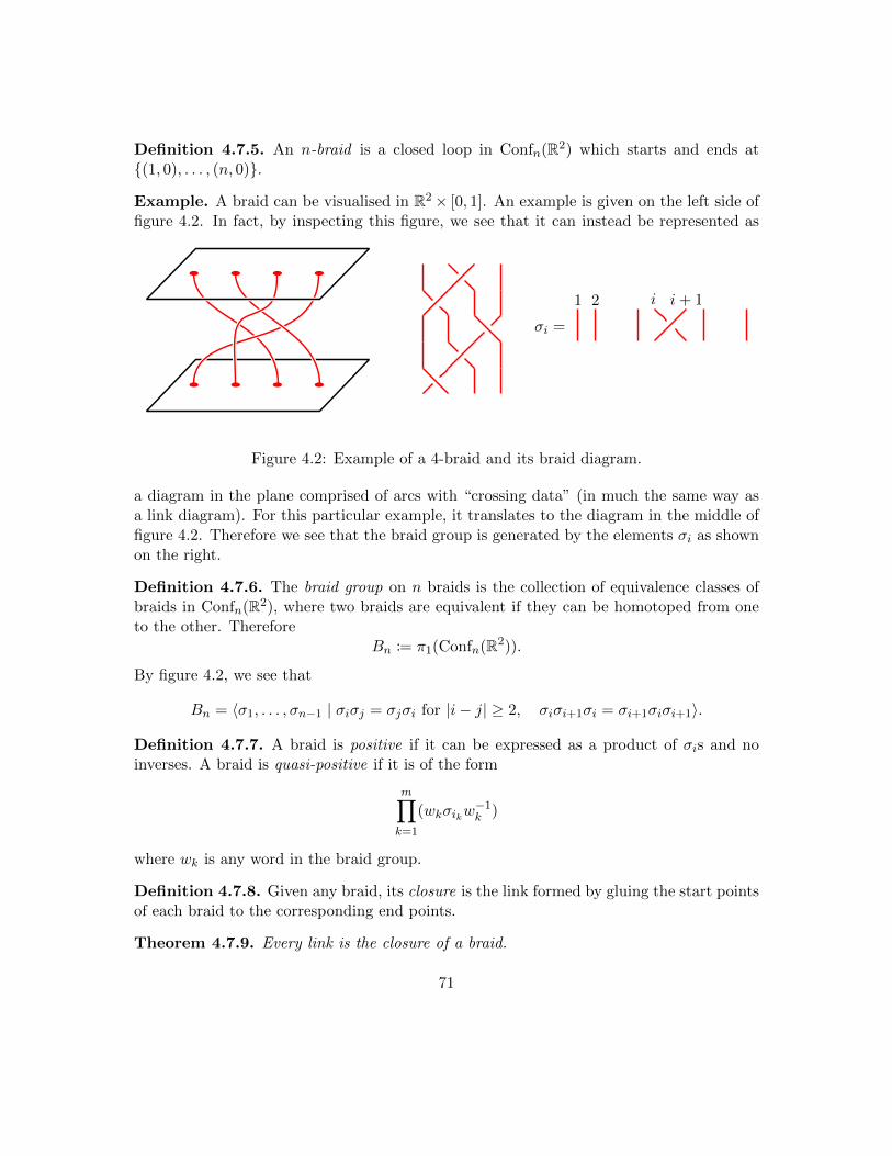
Definition 4.7.5. An n-braid is a closed loop in Confn(R2) which starts and ends at(1, 0), . . . , (n, 0).
Example. A braid can be visualised in R2× [0, 1]. An example is given on the left side offigure 4.2. In fact, by inspecting this figure, we see that it can instead be represented as
σi =
1 2 i i+ 1
Figure 4.2: Example of a 4-braid and its braid diagram.
a diagram in the plane comprised of arcs with “crossing data” (in much the same way asa link diagram). For this particular example, it translates to the diagram in the middle offigure 4.2. Therefore we see that the braid group is generated by the elements σi as shownon the right.
Definition 4.7.6. The braid group on n braids is the collection of equivalence classes ofbraids in Confn(R2), where two braids are equivalent if they can be homotoped from oneto the other. Therefore
Bn := π1(Confn(R2)).
By figure 4.2, we see that
Bn = 〈σ1, . . . , σn−1 | σiσj = σjσi for |i− j| ≥ 2, σiσi+1σi = σi+1σiσi+1〉.
Definition 4.7.7. A braid is positive if it can be expressed as a product of σis and noinverses. A braid is quasi-positive if it is of the form
m∏k=1
(wkσikw−1k )
where wk is any word in the braid group.
Definition 4.7.8. Given any braid, its closure is the link formed by gluing the start pointsof each braid to the corresponding end points.
Theorem 4.7.9. Every link is the closure of a braid.
71
Definition 4.7.10. A knot (or link) is called braid positive if it is the closure of a positivebraid. Similarly a knot (or link) is quasi-positive if it is the closure of a quasi-positivebraid.
Remark. We don’t call braid positive links “positive”, since they refer to oriented linkswith only positive crossings - a different notion.
Theorem 4.7.11 (Rudolph, Boileau-Orevkov). A knot K ⊂ S3 arises as K = S ∩ ∂B,with S ⊂ C2 an affine algebraic curve transverse to ∂B, if and only if K is quasi-positive.Moreover, in this instance, K bounds a complex curve of genus
g(S ∩B) =m− n+ 1
2,
provided that K = b, for b a quasi-positive n-braid of the form
b =
m∏k=1
wkσikw−1k .
Corollary 4.7.12. The slice genus of a quasi-positive knot K is gs(K) = (m− n+ 1)/2,with m and n as above.
Remark. The m and n above are not unique, but m − n is always fixed for any quasi-positive knot K.
Remark. For braid positive knots, it can be shown that u(K) = gs(K). However, forquasi-positive knots, this is not generally true. A counter example is given by the knot 820.
4.8 Donaldson diagonalisability theorem
We now give a proof of Donaldson’s diagonalisability theorem, which was instrumental inclassifying homeomorphism classes of 4-manifolds in terms of intersection forms. Recallthe following theorem from chapter 1 of the notes:
Theorem 4.8.1. Let X be a simply connected closed smooth 4-manifold. Then the home-omorphism class of X is determined uniquely by
σ(QX), parity(QX), χ(X).
The ingredients of this theorem are the classification of symmetric unimodular Z-bilinear forms, Freedman’s theorem, and Donaldson’s diagonalisability theorem.
Theorem 4.8.2 (Donaldson diagonalisability). Let X be a simply connected closed smooth4-manifold. Then if QX is definite, it is diagonal.
72
The original proof, in 1982, used Yang-Mills theory. Here we use Seiberg-Witten theoryto give a proof outline.
Proof. Suppose QX is negative definite. (Otherwise we can reverse the orientation of X.)Then b+2 = 0, so we cannot avoid reducibles among the solutions to the Seiberg-Wittenequations. Choose a metric and spinc-structure, and let c1(S+) = k be a characteristicelement of H2(X). Then we write
MSW = (A,Φ) solutions to SW, d?(A−A0) = 0, MSW = MSW /S1.
By transversality, for a generic perturbation η, MSW,η is a smooth manifold of dimension
d+ 1 =k2 − σ
4− b+2 + b1 =
k2 + b24
.
The second equality comes from the fact that QX is negative definite, so b2(X) = b−2 (X) =−σ(X). The d is the expected dimension of MSW .
Now we count the number of reducible solutions, by studying (A,Φ) such that Φ = 0,F+A = η, F+
A0+ d+(A−A0) = η. To solve for d+a = η − F+
A0, we inspect the sequence
Ω0 → Ω1 → Ω2+.
In this case H1 = H2+ = 0, so the equation d+a = η − F+
A0has a unique solution modulo
gauge (d? = 0). This means there is a unique reducible solution x.Now we study the geometry of MSW . away from the reducible solution, it’s a smooth
manifold of dimension d = 2m− 1. At the reducible solution, the local model is a cone onCPm−1 (since the reducible is a fixed point of the S1 action). Thus consider the smoothmanifold M∗SW =MSW − x. The S1 gives a line bundle L→M∗SW where
L[(A,Φ)] = (A, zΦ) : z ∈ C.
Then L|CP is the tautological bundle. But this almost gives a contradiction! Write c1(L) =u ∈ H2(M∗SW ). Then u restricted to CPm−1 is a generator of H2(CPm−1). Therefore um−1·[CPm−1] = 1. But this is nonsense, because CPm−1 bounds a cycle in M∗SW (namely thecomplement of a neighbourhood of the reducible solution x). This means that [CPm−1] =0 ∈ H2(M∗SW ), which is a contradiction! (Almost!)
This contradiction holds assuming m is positive. But m could be non-positive. In thiscase, M∗SW is empty, so MSW = x.
In summary it follows that m is necessarily negative, so that
m =k2 + b2
8≤ 0.
73
This rearranges to the requirement that k2 ≤ −b2. We now reduce to algebra: we have asymmetric unimodular Z-bilinear form
Q : Zr × Zr → Z, k2 + r ≤ for all k ∈ Char.
But now the proof reduces to a theorem of Elkies:
Theorem 4.8.3 (Elkies). If Q is a symmetric unimodular bilinear form with the aboveproperty, then Q is diagonal.
It follows that any simply connected closed smooth 4-manifold with a definite intersec-tion form has a diagonalisable intersection form.
4.9 Infinitude of smooth structures on K3.
We use Fintushel-Stern knot surgery to prove that the homeomorphism class of K3 surfacesadmit infinitely many smooth structures.
Definition 4.9.1. Fintushel-Stern knot surgery is the following procedure:
Fix a four manifold X, and a knot K. Suppose there is an embedding of a torusT 2 → X with “elliptic fibre”, that is to say [T 2]2 = 0 and [T 2] 6= 0.
Let N(T 2) denote a regular neighbourhood of T 2, which can be written as N(T 2) =T 2 ×D2 ⊂ X. Then ∂N(T 2) = T 2 × S1 = T 3.
Our knot K also determines a knot complement, which is S3 − N(K), for a regularneighbourhood N(K) = K × D2 of K. But then S1 × (S3 − N(K)) has boundaryS1 × ∂(S3 −N(K)) = S1 × ∂N(K) = T 3.
Since N(T 2) and S1×(S3−N(K)) have the same boundaries, we define the Fintushel-Stern knot surgery to be
XK = (X −N(T 2)) tT 3 (S1 × (S3 −N(K))).
There is a choice in the gluing: we send a meridian of K to ∗∂D2.
Theorem 4.9.2. If XK is obtained from a simply connected smooth manifold X by Fintushel-Stern knot surgery, then XK is homeomorphic to X.
Proof. Suppose X is simply connected. By Mayer-Vietoris and Seifert Van-Kampen, onecan show that for any K, π1(XK) = π1(X) = 1, and QXK = QX . Therefore by Freedman’stheorem, X is homeomorphic to XK .
74
Definition 4.9.3. Let X be a 4-manifold. The Seiberg-Witten series of X is the formalpower series
SWX =∑
k∈Char(X)
SWX(k)ek
where SWX is the Seiberg-Witten invariant of X.
Example. Let X be a K3 surface. Then c1(X) = 0, so SWX(0) = 1. In fact, SWX = 1.
Theorem 4.9.4 (Fintushel-Stern). Let XK be the smooth manifold obtained by Fintushel-Stern surgery along the knot K and torus T . Then
SWXK = SWX∆K(t), t = e2[T ].
In the above theorem, ∆K(t) denotes the Alexander polynomial with the “symmetricnormalisation” ∆(t) = ∆(t−1). Recall that the Alexander polynomial is characterised byskein relations:
∆0(t) = 1.
∆L+(t)−∆L−(t) = (t1/2 − t−1/2)∆L0(t).
Here L+, L−, and L0 correspond to the same link with a single crossing modified: L+ hasthe positive oriented crossing, L− the negative crossing, and L0 the un-crossing.
Example. The Alexander polynomial of the trefoil knot is t − 1 − t−1. The Alexanderpolynomial of Borromean rings is (t − 1)4, multiplied by some ±tk so that it becomes“symmetric” in the sense mentioned above.
Since the trefoil knot has Alexander polynomial t− 1− t−1, if XK is obtained from K3via Fintushel-Stern surgery along K = 31, then
SWXK = e2[T ] − 1 + e−2[T ].
I.e.
SWXK (s) =
1 if s = ±2[T ]
−1 if s = 0
0 otherwise.
Proposition 4.9.5. The Alexander polynomial satisfies the following properties:
∆K(t) = ∆K(−t)
∆K(1) = 1
All polynomials satisfying the above arise as ∆K(t) for some K.
75
Corollary 4.9.6. If K1,K2 are knots with distinct Alexander polynomials, then XK1 andXK2 are homeomorphic but not diffeomorphic.
Corollary 4.9.7. By the previous theorem, for a knot K, if XK is obtained by Fintushel-Stern knot surgery from K3 along K, then
SWXK = ∆K(t).
By the previous proposition there are infinitely many distinct Alexander polynomials, sothere are infinitely many smoothly distinct XK . But these are all homeomorphic to K3, sothe homeomorphism class of K3 admits infinitely many smooth structures.
Open question. Do there exist knots K1,K2 such that ∆K1(t) = ∆K2(t), but XK1 is notdiffeomorphic to XK2?
One easy way to obtain distinct knots with the same Alexander polynomial is to reflectthe knot. (e.g. the trefoil knot is chiral; i.e. not equivalent to its reflection.) However, inthis case the following results are known:
Proposition 4.9.8. Let K,Q be knots. Denote the reflection of K by K. Then for anyX, the manifolds XQ#K and XQ#K are diffeomorphic.
Note that the above holds when Q is the unknot, so XK∼= XK is a special case.
The Alexander polynomial is determined by the knot complement (which we can see inthe way that the Seiberg-Witten series is determined by the Alexander polynomial, whichitself comes from the knot complement). Moreover, one can show that the knot complementis an Eilenberg Maclane space,
S3 −N(K) = K(π1(S3 −K), 1).
Therefore the Seiberg-Witten invariant is determined by the fundamental group of the knotcomplement. This motivates the following open question:
Open question. Does π1(S3 −K) determine the diffeomorphism type of XK?
If this open question holds true, then diffeomorphism types of a given homeomorphismclass of a smooth manifold are at least as complicated as the fundamental groups of knotcomplements. Moreover, the following theorem holds:
Theorem 4.9.9. If K1,K2 are prime and have the same knot groups (i.e. the fundamentalgroups of their knot complements are isomorphic), then K1 = K2 or K1 = K2.
This means that fundamental groups of knot complements are at least as complicated asknots. Therefore if the previous open question holds true, we would have simply connectedsmooth 4-manifolds are at least as complicated as knots. That would be unfortunate froma classification viewpoint!
76
4.10 Furuta’s 10/8-theorem (lecture 14)
Suppose X4 is a smooth, closed, simply connected spin 4-manifold. (Recall that X admitsa spin structure if and only if QX is even.) Then
b2(X) ≥ 11
8|σ(X)|.
Equivalently,
QX = m
(0 11 0
)⊕ 2p(−E8),
with m ≥ 2p.
Proof. We give a proof sketch. The main ideas are as follows:
1. Study the Pin(2) symmetries of the solution space to SW. Construct a Pin(2)-equivariant “SW map”.
2. Extend the analysis of this map to Sobolev completions (which are easier to workwith in this case).
3. Construct and study finite dimensional approximations to the infinite dimensionalmap.
4. Use Furuta’s theorem on local properties of the approximations to more closely studythe SW map, to conclude the result.
1. Since QX is even, 0 is a characteristic element of X. Define a spinc structure s on X tobe a lift of the underlying spin structure. Then c1(s) = 0.
It follows that s = s, so the space of solutions to the SW equations is invariant underconjugation:
j : (A,Φ) 7→ (−A,Φ)
sends solutions to solutions. On the other hand, Gauge invariance ensures that the solutionspace is also invariant under
(A,Φ) 7→ (A, eiθΦ).
Combining these symmetries gives Pin(2) invariance of solutions to SW:
Pin(2) = S1 ∪ j · S1 ⊂ C⊕ jC = H.
Recall the map
SW : Γ(S+)⊕ Connections→ Γ(S−)⊕ Ω2+ ⊕ (Ω0/R)
defined bySW (Φ, A) = (DAΦ, F+
A − γ−1(ΦΦ∗)0, d
?(A−A0)).
77
This is Pin(2)-equivariant. We write this as
SW : H∞ ⊕ R∞ → H∞ ⊕ R∞,
where the Pin(2) is given by left multiplication on H∞, and its action on R is given by
S1 · x = x, j · x = −x.
2. To study this map, we want to work in the completions of the domain and codomainso that functional analysis can be applied. We begin by introducing some terminology.Let E → M be a vector bundle over a Riemannian manifold, where E is equipped withan inner product and connection. We denote the space of smooth sections by C∞(E), andthe kth Sobolev completion by L2
k(E). The kth Sobolev completion is the space of all ϕsuch that
∇iϕ ∈ L2, i ∈ 0, . . . , k.
The L2k norm is
‖ϕ‖2L2k
= ‖ϕ‖2 + · · ·+ ‖∇kϕ‖2.
Note that different metrics and connections give rise to equivalent norms. In our case, weobtain a map
SW : H = L2k(S
+ ⊕ T ∗X)→ H′ = L2k−1(S ⊕ Λ2
+T∗X ⊕ R)/R.
We can decompose this map into two pieces:
SW = `+ c, ` = dA0SW = (DA0 , d+ + d?).
Then ` is the linear part of SW , and c consists of the constant and quadratic terms. FromFredholm theory, we have
ind ` = dim ker `− dim coker ` =c1(s)2 − σ
4− b+2 .
This is realised by
indDA0 =c1(s)2 − σ
4= −σ
4, ind(d+ + d?) = −b+2 .
3. We now investigate finite dimensional approximations of SW : H → H′. Choose asequence of finite dimensional subspaces
coker ` ⊂ Vk ⊂ Vk+1 ⊂ · · · ⊂ H′,
such that⋃n Vn is dense in H′. (The subscript denotes the dimension.) Let Un = `−1(Vn).
The Sobolev completions are Hilbert spaces, so we have access to orthogonal projections.For each n, define
SWn = `+ projVnc : Un → Vn.
78
This is the “finite dimensional approximation” to SW .4. An important lemma by Furuta concerning the local structure of solutions is the
following:
Lemma 4.10.1. There exists R, ε > 0 such that for all sufficiently large n, if x ∈ Unsatisfies ‖x‖ < 2R, and |SWn(x)| < ε, then ‖x‖ < R.
The main idea is that SWn is a good approximation to SW on bounded sets. Fromthis theorem, we obtain a map
SW+
n : B(2R)/∂B(2R)→ B(ε)/∂B(ε)
defined by
x 7→
SWn(x) if |SW (x)| < ε
∗ otherwise.
Up to homotopy, this is a Pin(2)-equivariant map SW+
n : U+n → V +
n . As Pin(2) represen-tations, we can write Vn = Ha ⊕ Rb for some a and b. But now using finite dimensionalityand the index of `, we see that Un = Ha−σ/16 ⊕ Rb−b
+2 . Explicitly, this is because
ind ` = dim ker `− dim coker ` = dimUn − dimVn,
so writing QX = m
(0 11 0
)⊕ 2p(−E8) gives σ = −16p and b+2 = m. In summary, we
obtain a Pin(2)-equivariant map
f : (Ha+p ⊕ Rb−m)+ → (Ha ⊕ Rb)+.
The map has natural restrictions on the direct summands. Restriction onto the secondsummand gives a map
f : (0, a) 7→ (0, (d+ + d?)a), a = A−A0.
This is a linear map corresponding to the inclusion (Rb−m)+ → (Rb)+. The existenceof such a Pin(2)-equivariant map forces, essentially by the Borsuk Ulam theorem, thatm ≥ 2p+ 1. This implies the 10/8-theorem.
Recently (2018) the theorem was improved:
Theorem 4.10.2 (Hopkins, Lin, Shi, Xu). If X is a simply connected closed smooth 4-manifold, with n = 2p ≥ 4, then
m ≥
2p+ 2 p ≡ 1, 2, 5, 6
2p+ 3 p ≡ 3, 4, 7
2p+ 4 p ≡ 0
mod 8.
79
More precisely, it was shown using Pin(2)-equivariant stable homotopy theory that anymap as constructed at the end of the above proof exists if and only if
n ≥
2p+ 2 p ≡ 1, 2, 5, 6
2p+ 3 p ≡ 3, 4, 7
2p+ 4 p ≡ 0
mod 8.
Since this is a complete characterisation, it shows that this is the best possible result thatcan be obtained using Sieberg-Witten theory.
Open question. Is the “11/8”-theorem true? That is, if
QX = m
(0 11 0
)⊕ 2p(−E8),
then is m ≥ 3p?
If so, this would complete the classification of homeomorphism classes of simply con-nected smooth 4-manifolds.
4.11 Exotic smooth structures on R4
In this section, we prove the existence of an exotic smooth structure on R4. Later we givea proof outline that there are infact uncountably many distinct smooth structures on R4.
Our first example with arise from
X = CP2#9CP2.
Its intersection form is
QX = (1)⊕ 9(−1) ∼= (−E8)⊕ (−1)⊕ (1).
Denote by α an element of H2(X;Z) that spans the (1) term of QX . Suppose for acontradiction that α is represented by a smoothly embedded 2-sphere S2. We can then choosea D2-bundle over S2 with Euler number 1, so that the boundary of the neighbourhood isS3. Then this boundary realises a smooth connected sum
X = X ′#CP2, QX′ = (−E8)⊕ (−1).
But one can show that (−E8) ⊕ (−1) is not diagonalisable, despite being definite. Thiscontradicts Donaldson’s diagonalisability theorem, so X ′ cannot be smooth.
While α cannot be represented by a smoothly embedded sphere, it can actually berepresented by a topologically embedded sphere. This follows from Freedman’s theory: bygluing Casson handles onto disks, one can construct Σ ⊂ X such that Σ is a topologicalsphere representing α, and moreover Σ has a neighbourhood which smoothly embeds inCP2. Namely,
U ∼= CP2 −B4, U a neighbourhood of Σ.
80
Proposition 4.11.1. Z = CP2 − Σ is homeomorphic to R4, but not diffeomorphic.
Proof. We first establish that Z is not homeomorphic to R4 by using Freedman’s theoremfor open 4-manifolds. One can verify that π1(Z) = 1, and H∗(Z) = 0, using Seifert-vanKampen and Mayer-Vietoris. In particular, Z is contractible.
Next note that Z is “simply connected at infinity”. I.e. for all C ⊂ Z compact, thereexists D ⊂ Z compact with C ⊂ D such that π1(Z − D) → π1(Z − C) is trivial. In ourcase, Z ∩ U ∼= CP2 − B4 − CP1 = S3 × (0, 1). This is the “end” of Z. This is simplyconnected as required.
By Freedman’s theorem for open 4-manifolds, it follows that Z is homeomorphic to R4.
∼
Next we show that Z is not diffeomorphic to R4. Assume it is. Any compact subset of R4
can be enclosed in a smoothly embedded 3-sphere (i.e. given any C ⊂ R4 compact, we canwrite R4 = (R4 −B4) ∪B4, with C ⊂ B4.) In our case, let K = CP2 − U , where U is theneighbourhood defined earlier. Then K is compact. Suppose for a contradiction that K isenclosed in a smooth 3-sphere. Then
X ′′ = (X − nbhd(Σ)) ∪S3 B4
is a smooth simply connected manifold, with
QX′′ = (−E8)⊕ (−1).
But by Donaldson’s theorem, this is impossible!
Theorem 4.11.2. There uncountably many exotic R4s.
Proof. We give a proof outline. Above we verified the existence of one exotic R4, which wedenote by ER4. Let h : R4 → ER4 be a homeomorphism. Then write
h(B4(ρ)) = ER4ρ.
The refined theorem is the following:
Theorem 4.11.3. There exists ρ0 > 0 such that for all s > t > ρ0, ER4s is not diffeomor-
phic to ER4t .
Therefore our one example earlier provides an uncountable family. A proof sketchof the refined result is as follows: suppose ϕ : ER4
t → ER4s is a diffeomorphism. Let
h(S3(ρ)) = Yρ. Next choose x ∈ (t, s) and consider ϕ−1(Yx). This gives copies of Yx oneither side of Yt. By repeatedly gluing, we obtain a smooth 4-manifold “with periodic end”.One can conclude that the intersection form Q of this smooth manifold with periodic endis actually just QX−U = (−E8)⊕ (−1).
However, Taubes proved a version of Donaldson’s theorem for smooth manifolds withperiodic ends from which it follows that Q must be diagonalisable. This is a contradiction,so ϕ cannot exist.
81
Remark. The proof of Donaldson’s theorem for smooth manifolds with periodic ends usesYang-Mills theory. There is no known proof using Seiberg-Witten theory.
Question from class. Does the space of all smooth structures on R4 have any meaningfulstructure? topological or algebraic?
Answer. No, the above only gives a small family, in general we know nothing about whatthe space of all smooth structures looks like.
82
Chapter 5
Khovanov homology
The Khovanov homology is an intrinsically “combinatorial” invariant of knots. Using this,we will obtain the following:
A new proof of the Milnor conjecture (Rasmussen)
A new proof of the Thom conjecture (Lambert-Cole)
Existence of exotic R4s (Rasmussen-Gompf)
A possible approach to disprove the smooth 4-dimensional Poincare conjecture.
5.1 Definition of Khovanov homology (lecture 15)
Today we explore the definition and proof of invariance. We work with an oriented linkL ⊂ S3, with planar diagram D ⊂ R2. Recall that Reidemeister moves of link diagramscharacterise isotopy of links.
Proposition 5.1.1. The outline of Khovanov homology is as follows:
1. For each link diagram D, there is a corresponding cochain complex
D C(D) =⊕i,j∈Z
Ci,j(D).
This is equipped with boundary maps
d : Ci,j(D)→ Ci+1,j(D), d2 = 0.
2. We see that the index i gives the homological grading. On the other hand, the indexj defines the “quantum” or “Jones” grading.
83
3. The Khovanov homology is defined by
Kh•,•(L) = H•,•(C(D)) =⊕i,j
Khi,j(L).
We show that this is invariant under Reidemeister moves, and hence an invariant ofL.
Question from class. Are there any maps between the different Jones gradings?
Answer. Yes, we can define maps, but for our purposes we do not do this (yet).
Remark. In Russian, Khovanov is pronounced a little more like Hovanov. (Technicallythe kh is a voiceless velar fricative.) On the other hand, we see above that our theoryshould really be called a cohomology theory rather than a homology theory. Therefore itwould be more correct for our theory to be
Hovanov Khomology.
Why do we call the j index the “Jones” index? Given a chain complex, its Eulercharacteristic is defined to be
χ(H•(C)) =∑i
(−1)i rkH i(C).
For a bigraded complex, we modify this definition to obtain a Laurent polynomial. Inparticular, for the Khovanov homology,
χ(Kh•,•(L)) =∑i,j
(−1)iqj rk Khi,j(L) = JL(q) ∈ Z[q, q−1].
Remarkably, this Euler characteristic is an “unnormalised Jones polynomial”:
JL(q) = (q + q−1)JL(q2), for JL(t) the Jones polynomial.
Definition 5.1.2. Recall that the Jones polynomial is the polynomial invariant that trans-formed knot theory, characterised by the following skein relations:
J0(t) = 1.
t−1JL+(t)− tJL−(t) = (t1/2 − t−1/2)JL0(t).
Here L+, L−, and L0 correspond to the same link with a single crossing modified: L+ hasthe positive oriented crossing, L− the negative crossing, and L0 the un-crossing.
84
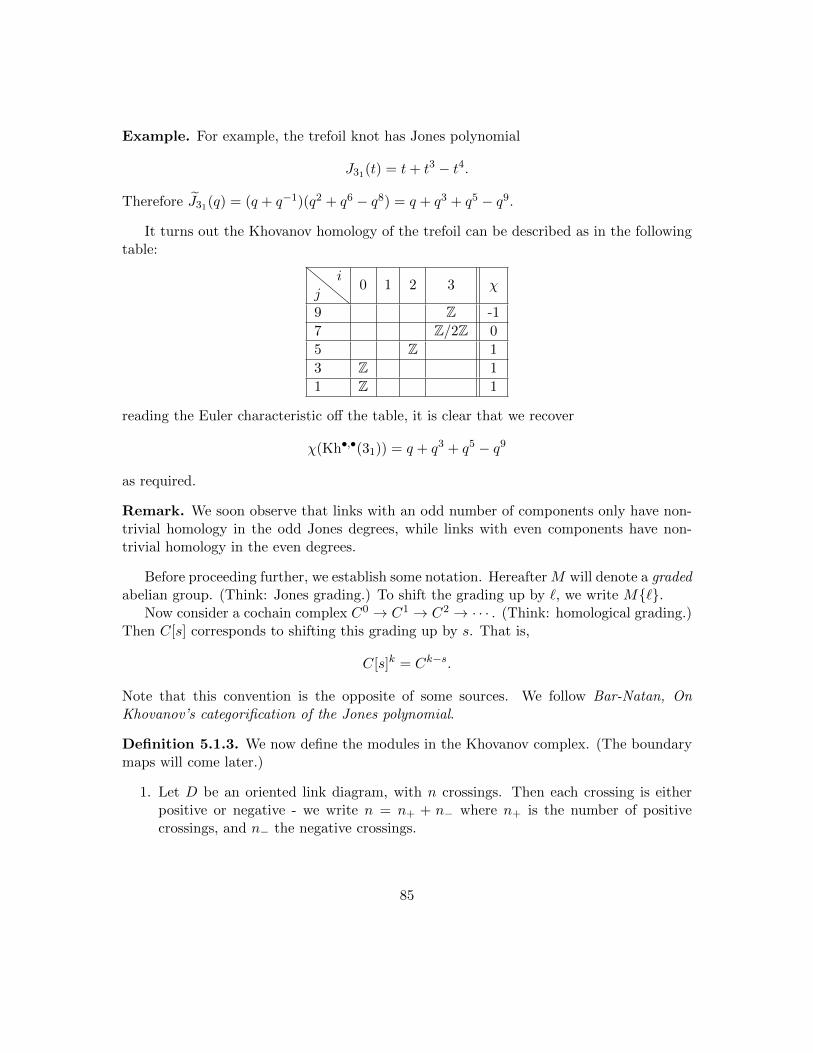
Example. For example, the trefoil knot has Jones polynomial
J31(t) = t+ t3 − t4.
Therefore J31(q) = (q + q−1)(q2 + q6 − q8) = q + q3 + q5 − q9.
It turns out the Khovanov homology of the trefoil can be described as in the followingtable:
ji
0 1 2 3 χ
9 Z -1
7 Z/2Z 0
5 Z 1
3 Z 1
1 Z 1
reading the Euler characteristic off the table, it is clear that we recover
χ(Kh•,•(31)) = q + q3 + q5 − q9
as required.
Remark. We soon observe that links with an odd number of components only have non-trivial homology in the odd Jones degrees, while links with even components have non-trivial homology in the even degrees.
Before proceeding further, we establish some notation. Hereafter M will denote a gradedabelian group. (Think: Jones grading.) To shift the grading up by `, we write M`.
Now consider a cochain complex C0 → C1 → C2 → · · · . (Think: homological grading.)Then C[s] corresponds to shifting this grading up by s. That is,
C[s]k = Ck−s.
Note that this convention is the opposite of some sources. We follow Bar-Natan, OnKhovanov’s categorification of the Jones polynomial.
Definition 5.1.3. We now define the modules in the Khovanov complex. (The boundarymaps will come later.)
1. Let D be an oriented link diagram, with n crossings. Then each crossing is eitherpositive or negative - we write n = n+ + n− where n+ is the number of positivecrossings, and n− the negative crossings.
85
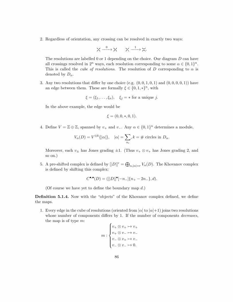
2. Regardless of orientation, any crossing can be resolved in exactly two ways:
0−−−→ 1−−−→ .
The resolutions are labelled 0 or 1 depending on the choice. Our diagram D can haveall crossings resolved in 2n ways, each resolution corresponding to some α ∈ 0, 1n.This is called the cube of resolutions. The resolution of D corresponding to α isdenoted by Dα.
3. Any two resolutions that differ by one choice (e.g. (0, 0, 1, 0, 1) and (0, 0, 0, 0, 1)) havean edge between them. These are formally ξ ∈ 0, 1, ∗n, with
ξ = (ξ1, . . . , ξn), ξj = ∗ for a unique j.
In the above example, the edge would be
ξ = (0, 0, ∗, 0, 1).
4. Define V = Z⊕ Z, spanned by v+ and v−. Any α ∈ 0, 1n determines a module,
Vα(D) = V ⊗k|α|, |α| =∑αi
, k = # circles in Dα.
Moreover, each v± has Jones grading ±1. (Thus v+ ⊗ v+ has Jones grading 2, andso on.)
5. A pre-shifted complex is defined by [|D|]r =⊕
α,|α|=r Vα(D). The Khovanov complexis defined by shifting this complex:
C•,•(D) = ([|D|]•[−n−]n+ − 2n−, d).
(Of course we have yet to define the boundary map d.)
Definition 5.1.4. Now with the “objects” of the Khovanov complex defined, we definethe maps.
1. Every edge in the cube of resolutions (oriented from |α| to |α|+1) joins two resolutionswhose number of components differs by 1. If the number of components decreases,the map is of type m:
m :
v+ ⊗ v+ 7→ v+
v+ ⊗ v− 7→ v−
v− ⊗ v+ 7→ v−
v− ⊗ v− 7→ 0.
86
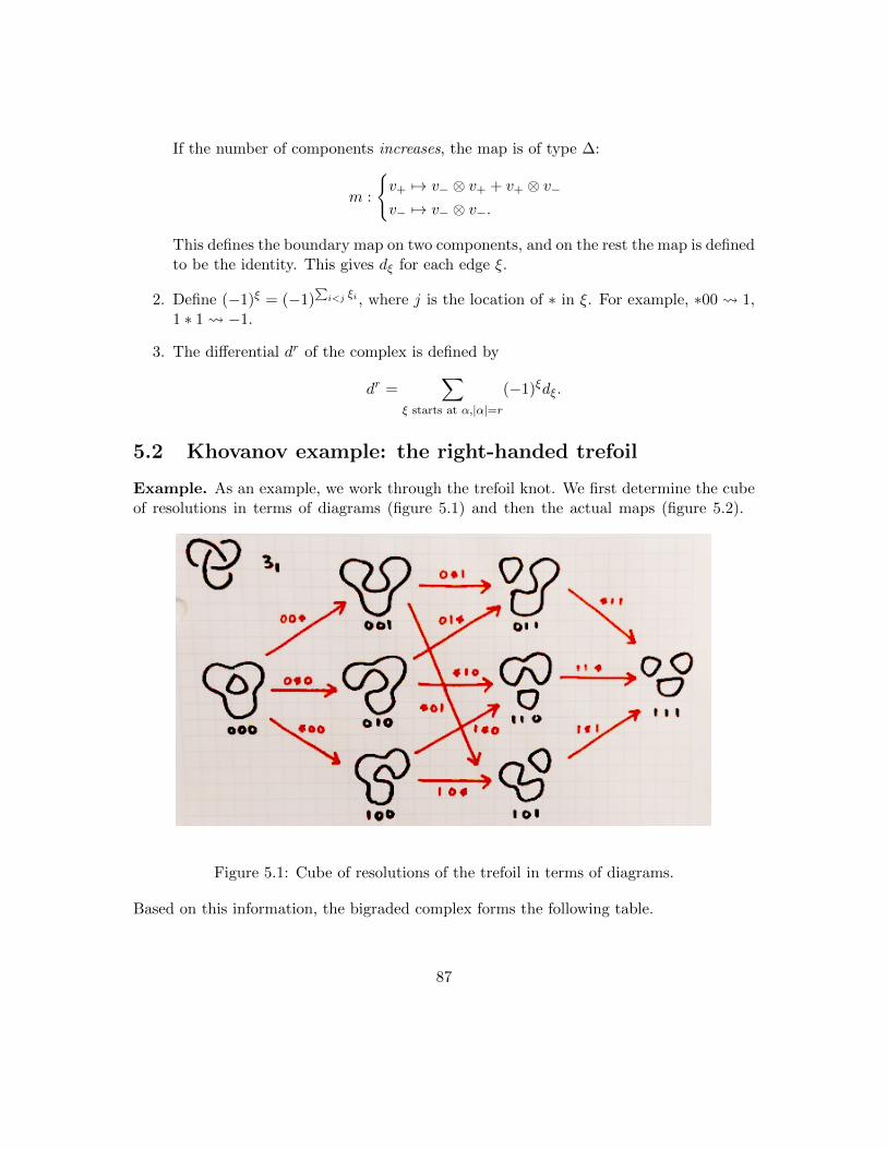
If the number of components increases, the map is of type ∆:
m :
v+ 7→ v− ⊗ v+ + v+ ⊗ v−v− 7→ v− ⊗ v−.
This defines the boundary map on two components, and on the rest the map is definedto be the identity. This gives dξ for each edge ξ.
2. Define (−1)ξ = (−1)∑i<j ξi , where j is the location of ∗ in ξ. For example, ∗00 1,
1 ∗ 1 −1.
3. The differential dr of the complex is defined by
dr =∑
ξ starts at α,|α|=r
(−1)ξdξ.
5.2 Khovanov example: the right-handed trefoil
Example. As an example, we work through the trefoil knot. We first determine the cubeof resolutions in terms of diagrams (figure 5.1) and then the actual maps (figure 5.2).
Figure 5.1: Cube of resolutions of the trefoil in terms of diagrams.
Based on this information, the bigraded complex forms the following table.
87
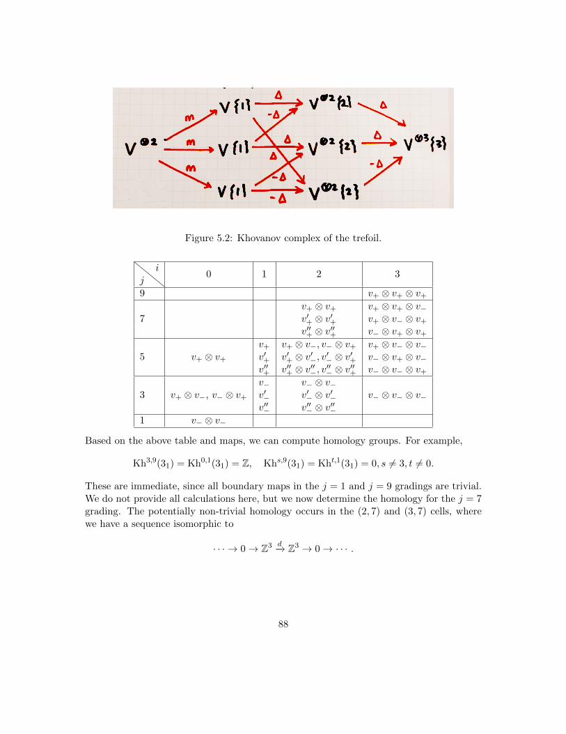
Figure 5.2: Khovanov complex of the trefoil.
ji
0 1 2 3
9 v+ ⊗ v+ ⊗ v+
v+ ⊗ v+ v+ ⊗ v+ ⊗ v−7 v′+ ⊗ v′+ v+ ⊗ v− ⊗ v+
v′′+ ⊗ v′′+ v− ⊗ v+ ⊗ v+
v+ v+ ⊗ v−, v− ⊗ v+ v+ ⊗ v− ⊗ v−5 v+ ⊗ v+ v′+ v′+ ⊗ v′−, v′− ⊗ v′+ v− ⊗ v+ ⊗ v−
v′′+ v′′+ ⊗ v′′−, v′′− ⊗ v′′+ v− ⊗ v− ⊗ v+
v− v− ⊗ v−3 v+ ⊗ v−, v− ⊗ v+ v′− v′− ⊗ v′− v− ⊗ v− ⊗ v−
v′′− v′′− ⊗ v′′−1 v− ⊗ v−
Based on the above table and maps, we can compute homology groups. For example,
Kh3,9(31) = Kh0,1(31) = Z, Khs,9(31) = Kht,1(31) = 0, s 6= 3, t 6= 0.
These are immediate, since all boundary maps in the j = 1 and j = 9 gradings are trivial.We do not provide all calculations here, but we now determine the homology for the j = 7grading. The potentially non-trivial homology occurs in the (2, 7) and (3, 7) cells, wherewe have a sequence isomorphic to
· · · → 0→ Z3 d−→ Z3 → 0→ · · · .
88
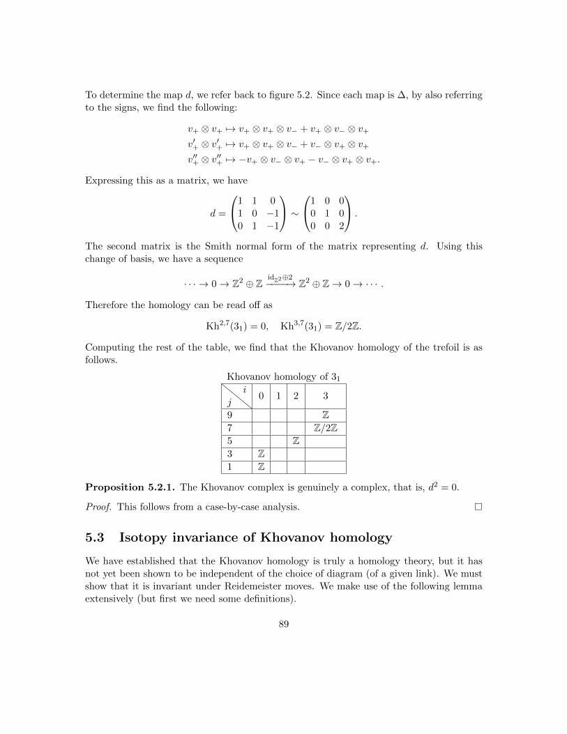
To determine the map d, we refer back to figure 5.2. Since each map is ∆, by also referringto the signs, we find the following:
v+ ⊗ v+ 7→ v+ ⊗ v+ ⊗ v− + v+ ⊗ v− ⊗ v+
v′+ ⊗ v′+ 7→ v+ ⊗ v+ ⊗ v− + v− ⊗ v+ ⊗ v+
v′′+ ⊗ v′′+ 7→ −v+ ⊗ v− ⊗ v+ − v− ⊗ v+ ⊗ v+.
Expressing this as a matrix, we have
d =
1 1 01 0 −10 1 −1
∼1 0 0
0 1 00 0 2
.
The second matrix is the Smith normal form of the matrix representing d. Using thischange of basis, we have a sequence
· · · → 0→ Z2 ⊕ ZidZ2⊕2−−−−→ Z2 ⊕ Z→ 0→ · · · .
Therefore the homology can be read off as
Kh2,7(31) = 0, Kh3,7(31) = Z/2Z.
Computing the rest of the table, we find that the Khovanov homology of the trefoil is asfollows.
Khovanov homology of 31
ji
0 1 2 3
9 Z7 Z/2Z5 Z3 Z1 Z
Proposition 5.2.1. The Khovanov complex is genuinely a complex, that is, d2 = 0.
Proof. This follows from a case-by-case analysis.
5.3 Isotopy invariance of Khovanov homology
We have established that the Khovanov homology is truly a homology theory, but it hasnot yet been shown to be independent of the choice of diagram (of a given link). We mustshow that it is invariant under Reidemeister moves. We make use of the following lemmaextensively (but first we need some definitions).
89
Definition 5.3.1. Let (C, d) be a complex, and C ′ ⊂ C a subcomplex. This means thatd(C ′) ⊂ C ′. This also gives rise to a quotient complex, C/C ′. We then obtain a short exactsequence
0→ C ′ → C → C/C ′ → 0
of complexes, which induces the usual long exact sequence on (co)homology
· · · → H i(C ′)→ H i(C)→ H i(C/C ′)→ H i+1(C ′)→ · · · .
Lemma 5.3.2. If C ′ is acyclic, i.e. if H∗(C ′) = 0, then H∗(C) ∼= H∗(C/C ′). Similarly ifH∗(C/C ′) = 0, then H∗(C ′) ∼= H∗(C).
This this notation established, we are ready to prove invariance under Reidemeistermoves. Invariance under those of types 2 and 3 are left as an exercise, but we proveinvariance of Khovanov homology under type 1 Reidemeister moves.
Proposition 5.3.3. Khovanov homology is invariant under type 1 Reidemeister moves.
Proof. Let D be a diagram with a crossing x that can be removed by a type 1 Reidemeistermove. Write [|D|] to denote the pre-shifted Khovanov complex of D. This factors as
C = [|D0|]m−→ [|D1|]1
where [|D0|] is a subcomplex which consists of all diagrams where x has a 0 resolution, and[|D1|] the subcomplex corresponding to x having the 1 resolution. Note that each diagram(vertex) in [|D0|] has an additional component L coming from the 0 resolution of x. On theother hand, the 1 resolution at x corresponds exactly to the type 1 Reidemeister move at x,so that [|D1|] is exactly the pre-shifted complex of D after applying a type 1 Reidemeistermove.
The component L contributes two free elements v+ and v−. Consider the subcomplexC ′ of C, where the space associated to L is restricted to the span of v+. Since the map mis defined by
m : v+ ⊗ w 7→ w,
we have an isomorphism
C ′ = [|D0|]v+ at Lm,∼=−−→ [|D1|]1.
The quotient complex C/C ′ is then given by
C/C ′ = [|D0|]v− at Lm−→ 0.
But [|D0|]v− at L is isomorphic to [|D′|]−1, where D′ is D after the type 1 Reidemeistermove has been applied. The shift −1 is to cancel the change in grading due to D′ havingone fewer crossing. But now by the previous lemma,
Kh(D) = [|D|]n+ − 2n− = [|D0|]v− at Ln+ − 2n− = [|D′|]n+ − 2n− − 1 = Kh(D′).
90
Proposition 5.3.4. The Khovanov homology is invariant under type 2 and type 3 Reide-meister moves.
Proof. These follow a similar argument. Details can be found in Dror Bar-Natan’s paper(which is available on the ArXiV).
5.4 Generalising Khovanov homology: TQFTs (lecture 16)
Recall that any crossing in a link diagram can be resolved in two ways, giving either the0 resolution or 1 resolution. If a link diagram is oriented, there is a unique way to resolveeach crossing so that it agrees with the orientation.
Given a link diagram D with c components, there are 2c possible orientations O, eachwith a unique resolution DO.
In the first section of today’s lecture, we explore the core of the invariance proofs of theprevious lecture to better understand Khovanov homology. A seemingly arbitrary choicewas that each component of a resolution was associated to Z⊕ Z, and the maps m and ∆were not motivated either.
We now attempt to better understand the underlying ingredients of Khovanov homol-ogy, independent of the choices.
1. The spaces were direct sums and tensor products of V = Z ⊕ Z. These had mapsm : V ⊗ V → V , and ∆ : V → V ⊗ V .
2. 1 ∈ V is a unit for m, and ε : V → Z defined by ε(v+) = 0 and ε(v−) = 1 is a counitfor ∆.
3. The map m itself is a commutative associative multiplication. ∆ is a cocommutativecoassociative comultiplication.
4. The maps satisfy the Frobenius law, ∆ m = (m⊗ 1) (1⊗∆).
These are exactly the ingredients of a commutative Frobenius algebra.
Proposition 5.4.1. To obtain a homological invariant of knots like Khovanov homology,we need V a commutative Frobenius algebra, free of rank 2.
The easiest way to think about commutative Frobenius algebras is to consider (1+1)-dimensional topological quantum field theories (TQFTs).
Theorem 5.4.2. There is an equivalence of groupoids
TQFTs 2Cob→ Vectk ←→ comFrobk.
We do not give a formal proof, but describe (1+1) dimensional TQFTs (i.e. functors2Cob → Vectk), and give examples of how they correspond to commutative frobeniusalgebras.
91

Remark. Here we describe TQFTs as functors into vector spaces, but in our context theyare abelian groups.
Definition 5.4.3. The category 2Cob consists of (1+1) dimensional cobordisms. Thatis, the objects are closed one-manifolds (disjoint unions of circles), and the morphisms arecobordisms between them.
Definition 5.4.4. Vectk is the category of vector spaces over a field k. A (1+1) dimen-sional TQFT is a functor that sends a 1-manifold to a vector space, and a cobordism toa homomorphism between them. Moreover, these respect the monoidal (tensor product)structure: for X,Y 1-manifolds,
Z(X t Y ) = Z(X)⊗ Z(Y ).
The following table describes the four generators of 2Cob, and how they correspondto maps in a Frobenius algebra.
M Z(M) Interpretation
1 : k → A unit
m : A⊗A→ A multiplication
ε : A→ k counit
∆ : A→ A⊗A comultiplication
Properties such as associativity, commutativity, and the Frobenius law can all be verifiedby using the classification of surfaces. We give one example here:
idA = Z( )
= Z
= Z
Z
= m (1⊗ idA).
92
Example. Khovanov homology can be expressed in a perhaps more intuitive form by usingthe perspective of Frobenius algebras. Write
V = Z[x]/(x2).
Define m : V ⊗ V → V to be the usual product on Z[x]/(x2). 1 is of course a unit. Themap ∆ : V → V ⊗ V defined by
∆(1) = 1⊗ x+ x⊗ 1, ∆(x) = x⊗ x
is a comultiplication, and ε : V → Z defined by
ε(1) = 0, ε(x) = 1
is a counit. This defines the Khovanov homology with the symbols v+ = 1 and v− = x.
Example. We can consider a deformation
V = Z[x]/(x2 − t),
over the ring Z[t]. Let 1 and ε be as above, and m the usual multiplication on V . Wedefine a modified comultiplication maps as follows:
∆(1) = 1⊗ x+ x⊗ 1, ∆(x) = x⊗ x+ t(1⊗ 1).
This also defines a Frobenius algebra. With the notation v+, v−, the multiplication andcomultiplication maps can be written as
m :
v+ ⊗ v+ 7→ v+
v+ ⊗ v−, v− ⊗ v+ 7→ v−
v− ⊗ v− 7→ tv+
∆ :
v+ 7→ v+ ⊗ v− + v− ⊗ v+
v− 7→ v− ⊗ v− + tv+ ⊗ v+.
This gives rise to a complex C ′(D) of Z[t]-modules. When t = 0 this is the Khovanovcomplex. When t = 1, this is the Lee complex, which we denote by CLee(D).
The corresponding integral homology theories are denoted by Kh(K) and Lee(K),called the Khovanov and Lee homologies respectively. We write Kh′(K) to represent theKhovanov-Lee homology over Z[t].
93
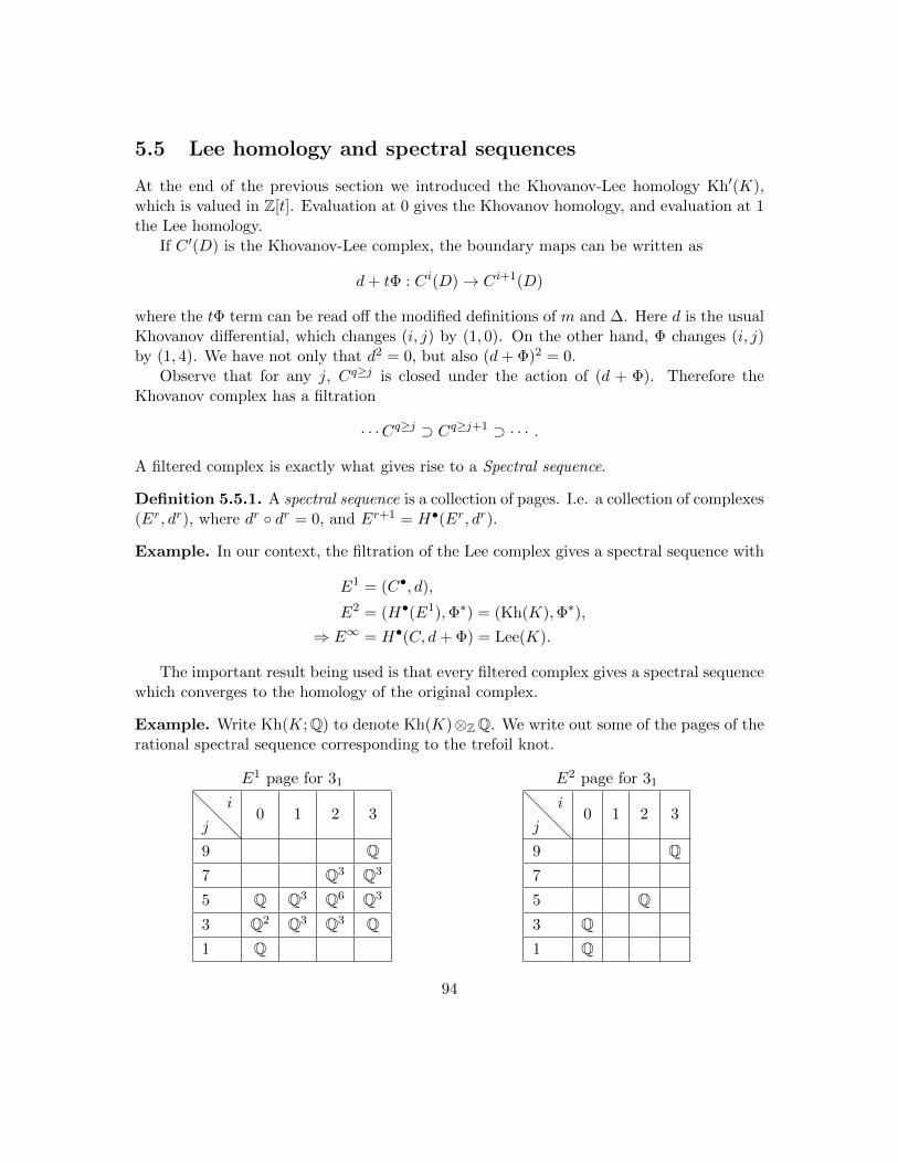
5.5 Lee homology and spectral sequences
At the end of the previous section we introduced the Khovanov-Lee homology Kh′(K),which is valued in Z[t]. Evaluation at 0 gives the Khovanov homology, and evaluation at 1the Lee homology.
If C ′(D) is the Khovanov-Lee complex, the boundary maps can be written as
d+ tΦ : Ci(D)→ Ci+1(D)
where the tΦ term can be read off the modified definitions of m and ∆. Here d is the usualKhovanov differential, which changes (i, j) by (1, 0). On the other hand, Φ changes (i, j)by (1, 4). We have not only that d2 = 0, but also (d+ Φ)2 = 0.
Observe that for any j, Cq≥j is closed under the action of (d + Φ). Therefore theKhovanov complex has a filtration
· · ·Cq≥j ⊃ Cq≥j+1 ⊃ · · · .
A filtered complex is exactly what gives rise to a Spectral sequence.
Definition 5.5.1. A spectral sequence is a collection of pages. I.e. a collection of complexes(Er, dr), where dr dr = 0, and Er+1 = H•(Er, dr).
Example. In our context, the filtration of the Lee complex gives a spectral sequence with
E1 = (C•, d),
E2 = (H•(E1),Φ∗) = (Kh(K),Φ∗),
⇒ E∞ = H•(C, d+ Φ) = Lee(K).
The important result being used is that every filtered complex gives a spectral sequencewhich converges to the homology of the original complex.
Example. Write Kh(K;Q) to denote Kh(K)⊗ZQ. We write out some of the pages of therational spectral sequence corresponding to the trefoil knot.
E1 page for 31
j
i0 1 2 3
9 Q7 Q3 Q3
5 Q Q3 Q6 Q3
3 Q2 Q3 Q3 Q1 Q
E2 page for 31
j
i0 1 2 3
9 Q7
5 Q3 Q1 Q
94
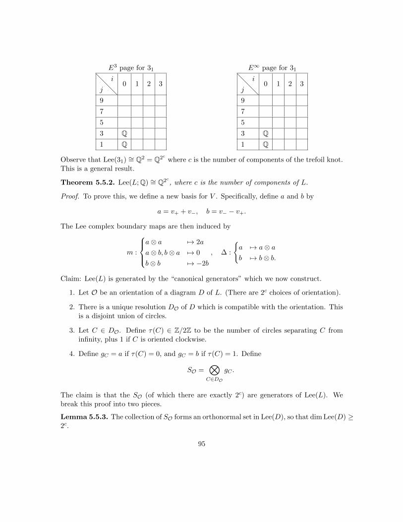
E3 page for 31
j
i0 1 2 3
9
7
5
3 Q1 Q
E∞ page for 31
j
i0 1 2 3
9
7
5
3 Q1 Q
Observe that Lee(31) ∼= Q2 = Q2c where c is the number of components of the trefoil knot.This is a general result.
Theorem 5.5.2. Lee(L;Q) ∼= Q2c, where c is the number of components of L.
Proof. To prove this, we define a new basis for V . Specifically, define a and b by
a = v+ + v−, b = v− − v+.
The Lee complex boundary maps are then induced by
m :
a⊗ a 7→ 2a
a⊗ b, b⊗ a 7→ 0
b⊗ b 7→ −2b
, ∆ :
a 7→ a⊗ ab 7→ b⊗ b.
Claim: Lee(L) is generated by the “canonical generators” which we now construct.
1. Let O be an orientation of a diagram D of L. (There are 2c choices of orientation).
2. There is a unique resolution DO of D which is compatible with the orientation. Thisis a disjoint union of circles.
3. Let C ∈ DO. Define τ(C) ∈ Z/2Z to be the number of circles separating C frominfinity, plus 1 if C is oriented clockwise.
4. Define gC = a if τ(C) = 0, and gC = b if τ(C) = 1. Define
SO =⊗C∈DO
gC .
The claim is that the SO (of which there are exactly 2c) are generators of Lee(L). Webreak this proof into two pieces.
Lemma 5.5.3. The collection of SO forms an orthonormal set in Lee(D), so that dim Lee(D) ≥2c.
95
We first note that if any two circles have the same label (either a or b) then they cannotmeet at a resolved vertex. It follows that each SO is a cycle, i.e. (d+ Φ)SO = 0. Therefore[SO] ∈ Lee(D).
Now that it has been established that these are all elements of Lee(D), we equip CLee(D)with an inner product by declaring that the a⊗a⊗ b⊗ · · · is an orthonormal basis. Themap d+ Φ has an adjoint with respect to the inner product, namely
(d+ Φ)∗ :
a⊗ a 7→ a
b⊗ b 7→ b
a 7→ 2a⊗ ab 7→ −2b⊗ brest 7→ 0.
Then one can show that (d + Φ)∗SO = 0. But this implies that each SO descends to anelement of Lee(D) while preserving pairwise orthogonality, since
Lee(D) = H∗(SLee(D)) = ker(d+ Φ)/ im(d+ Φ) ∼= ker(d+ Φ) ∩ ker(d+ Φ)∗.
In summary this proves that dim Lee(D) ≥ 2c.
Lemma 5.5.4. In fact, dim Lee(D) = 2c.
To see this, it remains to prove that dim Lee(D) ≤ 2c. This follows from an inductionon the number of crossings of D. Let D0 and D1 be 0 and 1 resolutions of a single crossing xin D. Then CLee(D1) ⊂ CLee(D) is a subcomplex. This gives rise to a long exact sequence
· · · → Lee(D1)→ Lee(D)→ Lee(D0)→ Lee(D1)→ · · · .
There are two cases to consider. First suppose the two strands crossing at x belong todistinct components of D. Then D0 and D1 each have c − 1 components each. By theinductive hypothesis,
dim Lee(D0) = dim Lee(D1) = 2c−1.
By the long exact sequence,
dim Lee(D) ≤ dim Lee(D0) + dim Lee(D1) = 2c−1 + 2c−1 = 2c.
This proves the first case. For the second case, suppose the strands meeting at x belongto the same component. Then one of D0, D1 has c components, and the other c + 1components. (Assume without loss of generality that D0 has c components, and D1 hasc+ 1 components.) The induced map
Lee(D0)i−→ Lee(D1)
is then injective. Therefore dim Lee(D) = dim coker i = 2c. (The size of the cokernel canbe verified by showing that the canonical generators of Lee(D0) map to half of those ofLee(D1).) The other case is formally dual, with a surjective map and so on.
This completes the proof that dim Lee(D) = 2c. Therefore Lee(D) = Q2c .
96
5.6 Rasmussen’s s-invariant (lecture 17)
Let K ⊂ S3 be a knot. Recall that the slice genus is the minimal genus of a surface boundby K in a 4-ball:
gs(K) := ming(Σ) : Σ ⊂ B4 properly smoothly embedded, ∂Σ = K.
Recall the Milnor conjecture (now a theorem), which we proved earlier using Seiberg-Wittengauge theory:
Theorem 5.6.1 (Milnor conjecture). Let K denote the p, q-torus knot, for p, q coprime.Then gs(K) = (p− 1)(q − 1)/2.
The original proof, due to Kronheimer and Mrowka in 1993, used Yang-Mills gaugetheory.
Several years later, Kronheimer and Mrowka proved the result using Seiberg-Wittengauge theory.
In 2004, Rasmussen gave a “combinatorial” proof. This is what we’ll start discussingtoday.
Recall that the slice genus is a lower bound for the unknotting number, and the p, q-torusknot K can be unknotted in (p− 1)(q − 1)/2 moves. Therefore
gs(K) ≤ u(K) ≤ (p− 1)(q − 1)
2.
On the other hand, today we introduce Rasmussen’s s-invariant s ∈ 2Z. We show that
1. |s(K)| ≤ 2gs(K).
2. s(K) = (p− 1)(q − 1).
Therefore by combining 1 and 2,
(p− 1)(q − 1)
2=s(K)
2≤ gs(K).
This will prove the Milnor conjecture.To give a definition of the s-invariant, we consider Khovanov and Lee homology with
rational coefficients. Recall that a diagram D for an arbitrary knot K determines a complex(C(D), d) called the Khovanov complex. This in turn determines a homology theory whichis invariant under Reidemeister moves, which we call the Khovanov homology Kh(K). By
97
perturbing the boundary maps, we obtain a different complex (CLee(D), d+ Φ) called theLee complex, and this also gives an invariant homology theory Lee(K). Moreover,
Kh(K)⇒ Lee(K) = Q⊕Q.
Although Lee(K) is almost trivial, the two surviving copies of Q have Jones (q) gradings.Let smax ≥ smin be the Jones gradings of the two copies. Since K is a knot, smax, smin areboth odd. Moreover, the isomorphism type of the spectral sequence is an invariant of K,so smax and smin are also invariants. It turns out that smax = smin + 2, so we define theRasmussen invariant to be
s(K) = smax(K)− 1 = smin(K) + 1 ∈ 2Z.
While this is the idea, we now give a formal definition of smax(K) and smin(K).
Definition 5.6.2. Let D be a diagram of a knot K. Then CLee(D) has a filtration
CLee(D) ⊃ · · · ⊃ Cq≥jLee (D) ⊃ Cq≥j+1Lee (D) ⊃ · · · ⊃ 0,
since the map d + Φ changes the bidegree (i, j) by (1, 0) (by d) and by (1, 4) (by Φ). Foreach j, we define
Ij = im(H∗(Cq≥jLee (D)) → H∗(CLee(D))) ⊂ Lee(D).
Note that there exists some N so that we need only consider −N ≤ j ≤ N for j as above.Then
Lee(D) = I−N ⊃ I−N+1 ⊃ · · · ⊃ IN = 0.
This induces a grading on Lee(D), by
Lee(D) =⊕j
Ij/Ij+1.
Now any class [x] in Lee(D) has a grading, namely
q([x]) = maxj : q(x) = j, x ∈ [x], q(x) = maxj : x ∈ Cq≥jLee (D).
In particular, we define
smax(K) = maxq([x]) : [x] ∈ Lee(K), [x] 6= 0, smin(K) = minq([x]) : [x] ∈ Lee(K), [x] 6= 0.
Given these formal definitions of the invariants smin and smax, the definition of theRasmussen invariant rests on the following result:
Proposition 5.6.3. Let K be a knot. Then smax(K) = smin(K) + 2.
98
Note that this justifies the definition of the Rasmussen invariant to be s(K) = smax−1 =smin + 1.
Proof. The main idea of the proof is to study the two canonical generators SO and SO ofLee(K) = Q⊕Q introduced in the previous lecture. We use combinations of these to firstshow that smax − smin ≡ 2 mod 4. (In particular, they differ by at least 2.) Whe theyshow that they differ by at most 2, to obtain the desired equality.
First note that for a knot K, we already know that CLee is supported only in oddquantum gradings. Define
CLee,even(D) = generated by elements with q = 1 mod 4
CLee,odd(D) = generated by elements with q = 3 mod 4
Note that d preserves the q grading while Φ changes it by 4, so d+ Φ preserves q modulo4. In particular, CLee(D) = CLee,even(D) ⊕ CLee,odd(D), where the direct summands arepreserved by d+ Φ. It follows that
Lee(K) = Leeeven(K)⊕ Leeodd(K).
We now make use of this direct summand structure. Define ι : CLee(D)→ CLee(D) to actby 1 on CLee,even, and -1 on CLee,odd. Then any x ∈ CLee(D) decomposes as
x =x+ ι(x)
2+x− ι(x)
2,
where the first term lives in CLee,even, and the second in CLee,odd. We further definei : V → V by i(v−) = v− and i(v+) = −v+. Then ι = ±i⊗n. Moreover, setting a = v−+v+
and b = v− − v+ as an alternative basis, we have i(a) = b and i(b) = a.We now analyse SO and SO more closely. These actually arise from the same diagram!
Switching all orientations in a diagram and then resolving gives rise to the same resolution,but with all orientations switched. Therefore
i([SO]) = ±[SO].
It follows that the canonical even/odd decomposition is given by
[SO] =[SO] + [SO]
2+
[SO]− [SO]
2.
This proves that the two copies of Q in Lee(K) = Q⊕Q live in different gradings mod 4,as required. That is,
smax − smin ≡ 2 mod 4.
In particular, smax is at least smin + 2.
99
Finally we show that smax is at most smin + 2. This follows from a similar calculationas showing that the Khovanov homology is invariant under Reidemeister moves. Let D′
denote the diagram of K obtained by adding a crossing via a type 1 move. Then
CLee(D′) =
(CLee(D t 0)→ CLee(D)
).
This can expressed as the short exact sequence
0→ CLee(D)→ CLee(D′)→ CLee(D t 01)→ 0
which induces a long exact sequence in homology
· · · → Lee(K)→ Lee(K)→ Lee(K t 01)∂−→ Lee(K)→ · · ·
where Lee(K t 01) ∼= Lee(K)⊗ V . Depending on labels near the crossing x of D′ obtainedfrom the type 1 move, we denote the two canonical generators of CLee(D) by sa and sb.Without loss of generality, q(sa − sb) = smax, and q(sa + sb) = smin. One can verify that
∂([sa − sb]⊗ [a]) = [sa],
from which it follows that
smax − 1 = q([sa − sb]⊗ [a]) ≤ q([sa]) + 1 = smin + 1.
Therefore smax ≤ smin + 2 as required. Earlier we established that smax ≥ smin + 2, so thiscompletes the proof that smax = smin + 2.
In summary the Rasumussen s-invariant is well defined.
5.7 The s-invariant bounds the slice genus
Recall that the proof strategy for proving Milnor’s conjecture is two establish the followingtwo facts:
1. |s(K)| ≤ 2gs(K).
2. s(K) = (p− 1)(q − 1).
We now prove the first of these.
Proposition 5.7.1. For a knot K, |s(K)| ≤ 2gs(K).
100
Proof. The idea is to use the functoriality of Khovanov-homology under link cobordisms.Let L0 and L1 be links, with Σ ⊂ R3 × [0, 1] a cobordism between them. We induce mapsFΣ : Kh(L0)→ Kh(L1), and FΣ,Lee : Lee(L0)→ Lee(L1) and use their properties.
By Morse theory, Σ splits into building blocks with one critical point each, of indices0,1, or 2. (These are with respect to the height function π : Σ → [0, 1].) If D0 is adiagram for L0, and D1 a diagram for L1, then D0 and D1 must be related by a sequenceof Reidemeister moves and Morse moves. By a Morse move, we mean the change in levelset as we pass a critical point. Explicitly,
Passing an index 0 critical point corresponds to taking a disjoint union with anunknot.
Passing an index 1 critical point corresponds to locally swapping two horizontal arcswith two vertical arcs or vice versa.
Passing an index 2 critical point corresponds to destroying a disjoint unknot.
Therefore to define a map FΣ : Kh(L0) → Kh(L1) we must define maps correspondingto each Reidemeister or Morse move, and glue them together. We must then verify thatthe map FΣ is an invariant of Σ, that is, it must not depend on the choice of Morsefunction/decomposition.
Explicitly, to each move, we associate the following maps:
For each Reidemeister move Di to Di+1, there is a canonical isomorphism Fi :Kh(Di)→ Kh(Di+1) as used in the proof of the well-definedness of Khovanov homol-ogy.
For an index 0 Morse move Di to Di+1 = Di t 01, define Fi : Kh(Di)→ Kh(Di+1) tosend 1 7→ v+ on the 01 component, and the identity elsewhere.
For an index 1 Morse move Di to Di+1, define Fi to be m or ∆ at the location ofthe move depending on the change in the number of components, and the identityelsewhere.
For an index 2 Morse move Di to Di+1, define Fi to send v− to 1 and v+ to 0 at thelocation of the move, and the identity elsewhere.
If D1, . . . , Dn are a sequence of diagrams from L0 to L1, the composition of the Fi definesthe map FΣ : Kh(L0)→ Kh(L1). We claim without proof that the map FΣ is well definedup to sign as an invariant of Σ. That is, the map does not depend on the decompositionof Σ. (This is a theorem of Khovanov and Jacobsson.) Note that this fact is not actuallyneeded for the proof!
A similar construction works for the Lee homology! We obtain maps FΣ,Lee : Lee(L0)→Lee(L1) as well.
101
Suppose Σ is an oriented cobordism from L0 to L1, such that every component of Σ hasa boundary component on L0. Then by verifying each Reidemeister and Morse move, onecan show that FΣ,Lee([SO|L0
]) is a non-zero multiple of [SO|L1], where O is an orientation
of Σ. This means that if Σ is a connected cobordism between knots K0 and K1, thenFΣ,Lee : Q⊕Q→ Q⊕Q is an isomorphism.
Suppose Σ has genus g = gs(K) for a knot K. Then removing a disk D, Σ′ = Σ−D is agenus g cobordism from K to the unknot. Now FΣ and FΣ,Lee are maps from Khovanov andLee homologies of K to that of the unknot. How do they change the quantum gradings?Observe that Reidemeister moves leaves q invariant, while Morse moves of index 0 and 2change q by +1, and Morse moves of index 1 change q by −1. Therefore FΣ changes q byχ(Σ′), and FΣ,Lee by at least χ(Σ′).
Let x ∈ Lee(K)− 0 be a class attaining q(x) = smax = s+ 1. Then
1 ≥ q(FΣ′(x)) ≥ q(x) + χ(Σ′) = s+ 1− 2gs(K).
The first inequality is because FΣ′(x) lives in Lee(01). Therefore
s ≤ 2gs(K)
as required.Finally for the general result, consider the mirror K of K. This bounds a surface Σ
with the same genus as Σ. But now s(K) = −s(K), so
−s(K) ≤ 2g = 2gs(K).
Combining this with the previous result, we can bound gs(K) below by |s(K)|/2 as required.
5.8 Combinatorial proof of Milnor’s conjecture (lecture 18)
In the previous lecture we defined the Rasmussen s-invariant for knots, and showed thatit satisfies
|s(K)| ≤ 2gs(K).
Today we show that s(Tp,q) = (p− 1)(q − 1). This will be a special case of the calculationof s for positive knots.
Definition 5.8.1. A knot K is positive if it has an oriented diagram with only positivecrossings.
For example, a torus knot is a positive knot.
Remark. This notion is distinct from that of braid-positivity we introduced several lec-tures ago.
102
If D is a positive diagram of a positive knot, then its oriented resolution D0 is in factthe zero resolution! Our final result needed to prove the Milnor conjecture is the following:
Proposition 5.8.2. If K has a positive diagram D with n crossings, and D0 consists of kcircles (components), then s(K) = n+ 1− k.
Proof. Recall from the previous lecture that the s-invariant has the explicit formula
s(K) = s =q([SO] + [SO]) + q([SO]− [SO])
2.
Here one of [SO]± [SO] has degree s+ 1, and the other has degree s− 1. Moreover,
q([SO]) = q([SO]) = s− 1.
Explicitly, the left side is defined to be
q([SO]) = maxq(x) : x is homologous to SO = maxq(x) : x = SO + dα.
But SO lives in the lowest homological grading (since our resolution D0 is the zero resolu-tion). Therefore there is no non-trivial α that can map to dα, i.e. there is a unique classhomologous to SO. Hence
q([SO]) = q(SO), SO = (v+ ± v−)⊗ (v+ ± v−)⊗ · · · .
The expression on the right has k factors. But this necessarily lies in the same quantumgrading as ⊗kv−. Therefore by the definition of the Khovanov homology,
q(SO) = −k + (n+ − 2n−) = n− k = s− 1.
The claimed result follows.
Example. The standard diagram of the torus knot Tp,q consists of p(q− 1) positive cross-ings, and its 0 resolution consists of q circles. Therefore s(Tp,q) = p(q − 1) − q + 1 =(p− 1)(q − 1).
We can now pull together a proof of Milnor’s conjecture using just Rasmussen’s s-invariant.
Proposition 5.8.3. The slice genus of the torus knot Tp,q is
gs(Tp,q) =(p− 1)(q − 1)
2.
Proof. The standard diagram can me unknotted in (p− 1)(q − 1)/2 moves, giving
gs(Tp,q) ≤ u(Tp,q) ≤(p− 1)(q − 1)
2.
Conversely, the Rasmussen s-invariant gives
(p− 1)(q − 1)
2=s(Tp,q)
2≤ 2gs(Tp,q)
2= gs(Tp,q).
Therefore we have equality as required.
103
5.9 Combinatorial proof of the existence of exotic R4s
Another application of Khovanov homology is that it gives a novel proof of the existenceof exotic smooth structures on R4, without requiring any gauge theory. More concretely,our proof outline is as follows:
1. Use Rasmussen’s s invariant together with a result of Freedman to find knots thatare topologicall slice but not slice.
2. Introduce the trace embedding lemma.
3. Use the trace embedding lemma with manifolds obtained from a knot as in 1 toconstruct an open manifold which is homeomorphic to R4 but cannot be diffeomorphicto it. A result of Freedman states that all open 4-manifolds admit admit smoothstructures, so it must then be an exotic R4.
We now carry out the details. First we introduce relevant definitions and results to establishpoint 1.
Definition 5.9.1. A knot K is slice (or smoothly slice) if gs(K) = 0. That is, if thereexists a smooth properly embedded disk D ⊂ B4 such that ∂D = K ∈ S3.
By replacing the notion of a smooth embedding with a topological embedding, weobtain a weaker condition.
Definition 5.9.2. A knot K is topologically slice if there exists a locally flat topologicallyembedded disk D ⊂ B4 such that ∂D = K ∈ S3. This means that there is a topologicalembedding ϕ : (D2 ×D2, ∂D2 ×D2)→ (B4, ∂B4 = S3) such that ϕ(∂D2 × 0) = K. Thenϕ(D2 × 0) is a topologically embedded disk which is locally flat.
Remark. The local flatness condition is necessary to obtain an “interesting” definition:without this assumption, all knots would be topologically slice by taking the embeddeddisk to be a cone over the knot.
We now use the following theorem of Freedman to establish the existence of topologicallyslice knots which aren’t slice:
Theorem 5.9.3. If ∆K(t) = 1, then K is topologically slice.
Here ∆ is the Alexander polynomial. One method of proliferating knots with trivialAlexander polynomials is to take the Whitehead double Wh(K) of a knot K. In particular,
∆Wh(T2,3) = 1.
However, we can also compute the s-invariant for any given knot - this particular knotsatisfies s(Wh(T2,3)) = 2. Since s/2 is a lower bound for the slice genus, we know thatgs(Wh(T2,3)) ≥ 1. Therefore Wh(T2,3) is not slice, despite being topologically slice!
104
Remark. In fact, Wh(T2,3) = 0. This is because the “clasp” in the Whitehead doubleis not mirrored, i.e. the Mirror of a Whitehead double is not the Whitehead double of amirror. In general, it is known that all Whitehead doubles of torus knots are not slice, butsuch a result is not known for mirrors of torus knots!
The next ingredient in our proof of the existence of exotic smooth structures on R4
is the trace embedding lemma. This relates the properties of being slice (or topologicallyslice) to embeddings of “traces of 0 surgeries of knots”.
We establish some notation. Let K be a knot, and S3n(K) the manifold obtained by
n-surgery along K ⊂ S3. Let Xn(K) be the manifold obtained from B4 by attaching ann-framed 2-handle along K. Then Xn(K) is called the trace of the n-surgery along K, andsatisfies ∂Xn(K) = S3
n(K). Alternatively Xn(K) can be thought of a cobordism from S3
to S30(K) (with the S3 end capped).
Example. If K is the unknot, then S30(K) = S1 × S2, and X0(K) = (D2 × S2)−B4.
The trace embedding lemma takes two forms for each notion of sliceness:
Proposition 5.9.4. K ⊂ S3 is (topologically) slice if and only if X0(K) embeds smoothly(locally flat topologically) in S4.
We only prove the smooth case, as the locally flat case is similar.
Proof. ⇒. If K is slice, it bounds a disk D smoothly embedded in B4. One can verify that
S4 = X0(K) tS30(K) (B4 − int(nbhd(D))).
In particular, X0(K) embeds smoothly in S4.⇐. We start by constructing an embedding F : S2 → X0(K), so that F (S2) is of the
form D tK C where D is a smooth disk (and the core of the 2-handle of X0(K)) and Chas a single cone point. By assumption, there is a smooth embedding i : X0(K) → S4.Therefore we have an embedding iF : S2 → S4 which is smooth away from the cone point.Removing a small ball around the cone point, the image of i F restricts to a smoothlyembedded disk in B4, whose boundary is K.
The final step is to combine this result with the previous example of a non-slice topo-logically slice knot to construct an exotic R4.
Theorem 5.9.5. There exist exotic R4s.
Proof. Let K be a topologically slice knot which is not slice. Write
S4 = X0(K) ∪ (B4 − nbhd(D))
105
where D is a topologically flat disk, with boundary K. Define
Z = S4 − x − int(X0(K)) = R4 − int(X0(K)).
This is an open topological 4-manifold with boundary. A theorem of Freedman states thatall open 4-manifolds admit smooth structures, so we equip Z with a smooth structure. Inparticular ∂Z is a smooth manifold.
On the other hand, we already know that ∂Z is homeomorphic to ∂X0(K), which ishomeomorphic to S3
0(K). In dimension 3, all topological manifolds admit a unique smoothstructure, so ∂Z is diffeomorphic to S3
0(K). Now define
R = Z tϕ X0(K)
where ϕ : ∂Z → S30(K) is a diffeomorphism. This is a smooth manifold, and by Mayer-
Vietoris and Seifert-van Kampen, can be shown to be homeomorphic to R4.In particular, X0(K) embeds smoothly in R. Since K is not slice, X0(K) cannot embed
smoothly in R4. Therefore the smooth structure on R must be distinct from that on R4.This completes the proof.
5.10 FGMW strategy to disprove SPC4
In the previous proof, it was crucial that Z was open. This is because Freedman’s proof ofthe existence of smooth structures (on an arbitrary manifold) works everywhere except fora single point. Can we modify the approach to find exotic smooth structures of non-openmanifolds? What about shedding light on the smooth Poincare conjecture in dimension 4?
We now describe an equivalent formulation of the smooth Poincare conjecture in 4dimensions, and show how we can attempt to understand it using Khovanov homology aswe did above.
Proposition 5.10.1. The smooth Poincare conjecture in dimension 4 (SPC4) is equivalentto the statement that if W 4 is smooth with ∂W = S3 and W contractible, then W isdiffeomorphic to B4.
The equivalence is immediate. To get from S4 to W , simply remove a 4-ball, and toget from W to S4, glue along a 3-sphere (since we know that the 3-dimensional Poincareconjecture holds).
The Freedman-Gompf-Morrison-Walker (FGMW) strategy for disproving the smoothPoincare conjecture is as follows: find a knot K such that K bounds a smooth disk in someW contractible with ∂W = S3, s(K) 6= 0. Then K is not slice, so W 6= B4. Thus W is anexotic B4, which gives us an exotic S4.
Example. Earlier in the class we considered potential counter-examples to SPC4. Theycan be revisited here: can we find knots K as above in our potential SPC4 counter exam-ples?
106

Example. Suppose W has a handle decomposition with no 3-handles. The attachingspheres of 2-handles are in fact knots in S3, and moreover bound smooth disks in W(specifically the cores of the handles). Therefore if any of these K have non-trivial s-invariant, we are done. So far all such K have had trivial s-invariant.
Remark. There are invariants similar to the s-invariant that arise from Seiberg-Wittenand Yang-Mills gauge theory, along with Floer homology theories. However, none of thesecan distinguish between sliceness in B4 vs sliceness in homotopy B4s, so these cannot workin a similar strategy.
Whether or not this strategy has a chance of working is an open question. Moreprecisely, the following problem is open:
Open question. Let K ⊂ S3 = ∂W 4. Suppose W is smooth and contractible. SupposeΣ →W is a smooth proper embedding, with ∂Σ = K. Do we necessarily have
|s(K)| ≤ 2g(Σ)?
This is of course true if W = B4. If it is true for all W as above, then the FGMWstrategy fails.
Theorem 5.10.2 (Manolescu, Marengon, Sarkar, Willis). The inequality |s(K)| ≤ 2g(Σ)holds as above if W is a Gluck twist of a sphere.
As a corollary, the FGMW strategy fails for Gluck twists. We prove this in the lastlecture.
Recall the following definition of a Gluck twist:
Definition 5.10.3. Let X be a 4-manifold, and S2 → X an embedding with image S.Then there is a neighbourhood of S diffeomorphic to S2 ×D2. Then the Gluck twist of Xby S is
XS = (X − nbhd(S)) tϕ (S2 ×D2)
where ϕ : S2 × S1 → S2 × S1 is the map
ϕ : (z, eiθ) 7→ (rotθ(z), eiθ).
Question from class. Can Khovanov homology prove that there are infinitely manysmooth exotic structures on R4?
Answer. Yes. Consider distinct knots which are topologically slice but not slice. There isanother invariant such that if the two knots are distinguished by this invariant, then theyinduce different smooth structures. This cannot prove that there are uncountably manyexotic smooth structures however, since there are only countably many knots!
107
5.11 The FGMW strategy fails for Gluck twists (lecture 19)
In the previous lecture we introduced the Freedman-Gompf-Morrison-Walker strategy todisprove the smooth Poincare conjecture. It is an open question whether or not the strategycan be carried out. However, today we give a proof outline to show that the strategy failsfor Gluck twists.
Theorem 5.11.1 (Theorem A - Manolescu, Marengon, Sarkar, Willis). Let K ⊂ S3 = ∂W ,where W is obtained as a Gluck twist of B4. Suppose Σ →W is a smooth embedding, with∂Σ = K. Then |s(K)| ≤ 2g(Σ).
This means that if W is a smooth manifold homeomorphic to B4 obtained via a Glucktwist, and K is a knot bounding a disk in W , we cannot show that K is not slice (andhence W is not diffeomorphic to B4) by using the s-invariant. In other words, the FGMWstrategy fails for such W .
It is interesting that such a result can be proven, since we expect to only know infor-mation about cylinders S3 × [0, 1] based on the definition of the Khovanov homology.
Recall that Gluck twist, in our context, is the following manifold: let Σ ∼= S2 → B4
be an embedding. Then there is a neighbourhood N of Σ diffeomorphic to S2 ×D2. TheGluck twist of B4 by Σ is
W = B4Σ = (B4 −N) tϕ N
where ϕ : ∂N = S2 × S1 → S2 × S1 is the map
ϕ : (z, eiθ) 7→ (rotθ(z), eiθ).
It is known that a Gluck twist of B4 is homeomorphic to B4, but not if it is diffeomorphic.
Definition 5.11.2. GΣ denotes the Gluck twist of S4 by an embedding Σ → S4, withS2 ∼= Σ. By the following remark, there is no ambiguity in writing GΣ.
Remark. The diffeomorphism ϕ ∈ Aut(∂N) is a generator of π1(RP3) = π1(SO(3)) =S1 → rot(S2) = Z/2Z. If two maps in Aut(∂N) are homotopic, they give the same Glucktwists.
The proof outline for the MMSW theorem is as follows:
1. Prove a special case with W = CP2 −B4.
2. Prove a special case with W = CP2 −B4.
3. Use Kirby diagrams to prove a result analogous to the “stable diffeomorphism” clas-sification of 4-manifolds. Concretely, we show that GΣ#CP2 is diffeomorphic to CP2,
and GΣ#CP2 is diffeomorphic to CP2.
4. We combine the three results to prove the general result.
108
We now state and prove the first special case:
Proposition 5.11.3. “Theorem B”. Let W = CP2 − B4, and K ⊂ ∂W = S3. LetΣ ⊂ W be smoothly properly embedded, with ∂Σ = K. Suppose [Σ] = 0 ∈ H2(W,∂W ) =
H2(CP2) = Z. Then s(K) ≤ 2g(Σ).
Proof. The goal is to reduce the problem further to a surface in a cylinder. In that casewe obtain a map corresponding to the surface (as described in an earlier lecture).
Consider the data of W = CP2 − B4, K ⊂ ∂W = S3, and Σ ⊂ W smoothly properlyembedded, with ∂Σ = K and [Σ] = 0 ∈ H2(W,∂W ). Note that H2(W,∂W ) is generated
by [CP1].
Let N be a regular neighbourhood of CP1. Then ∂N = S3. Moreover, the “radial”
projection ∂N → CP1 ∼= S2 is the (negative) Hopf fibration. Decomposing along theboundary of N , we then have
CP2 = N t∂N (S3 × [0, 1]) t∂W B4.
We also assume that [Σ] = 0 ∈ H2(W,∂W ). Therefore [Σ] · [CP1] = 0. That is, assuming
transversality, Σ and CP1 intersect at 2p points, p positively signed and p negatively signed.Therefore Σ intersects N along 2p disks, and intersects ∂N along 2p circles. Each of thesecircles is a fibre of the negative Hopf fibration mentioned above.
The collection of fibres forms a link Lp,p ⊂ S3 in the total space of the Hopf fibration.In fact, this is a torus link T2p,2p with p strands oriented in one direction and p the otherway.
One can define Rasmussen’s s-invariant for links rather than just knots. Recall thatdim Lee(L) = 2` where L has ` components, and Kh(L) ⇒ Lee(L). This time there aremany generators, but our link has a given orientation, so there exist canonical generatorsSO and SO. We can define the s-invariant to be
s(L) =q([SO] + [SO]) + q([SO]− [SO])
2.
By the definition of Σ, its restriction to S3 × [0, 1] is a cobordism inside S3 × [0, 1] from Kto Lp,p, of genus g(Σ). By functoriality of the Khovanov homology under cobordisms (asin Rasmussen’s proof of the Milnor conjecture), we find that
s(K)− 2g(Σ) + 1− 2p ≤ s(Lp,p).
We can compute s(Lp,p). (This takes some work and is the main content of the paper byMMSW), but these turn out to be 1− 2p. Therefore the inequality above gives the desiredresult.
It is now straight forward to prove the result for CP2 instead of CP2. Explicitly, wehave the following proposition:
109
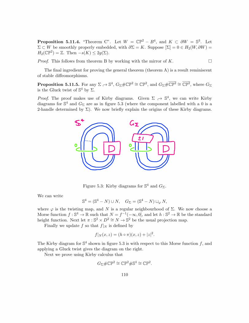
Proposition 5.11.4. “Theorem C”. Let W = CP2 − B4, and K ⊂ ∂W = S3. LetΣ ⊂ W be smoothly properly embedded, with ∂Σ = K. Suppose [Σ] = 0 ∈ H2(W,∂W ) =H2(CP2) = Z. Then −s(K) ≤ 2g(Σ).
Proof. This follows from theorem B by working with the mirror of K.
The final ingredient for proving the general theorem (theorem A) is a result reminiscentof stable diffeomorphisms.
Proposition 5.11.5. For any Σ → S4, GΣ#CP2 ∼= CP2, and GΣ#CP2 ∼= CP2, where GΣ
is the Gluck twist of S4 by Σ.
Proof. The proof makes use of Kirby diagrams. Given Σ → S4, we can write Kirbydiagrams for S4 and GΣ are as in figure 5.3 (where the component labelled with a 0 is a2-handle determined by Σ). We now briefly explain the origins of these Kirby diagrams.
Figure 5.3: Kirby diagrams for S4 and GΣ.
We can writeS4 = (S4 −N) ∪N, GΣ = (S4 −N) tϕ N,
where ϕ is the twisting map, and N is a regular neighbourhood of Σ. We now choose aMorse function f : S4 → R such that N = f−1(−∞, 0], and let h : S2 → R be the standardheight function. Next let π : S2 ×D2 ∼= N → S2 be the usual projection map.
Finally we update f so that f |N is defined by
f |N (x, z) = (h π)(x, z) + |z|2.
The Kirby diagram for S4 shown in figure 5.3 is with respect to this Morse function f , andapplying a Gluck twist gives the diagram on the right.
Next we prove using Kirby calculus that
GΣ#CP2 ∼= CP2#S4 ∼= CP2.
110
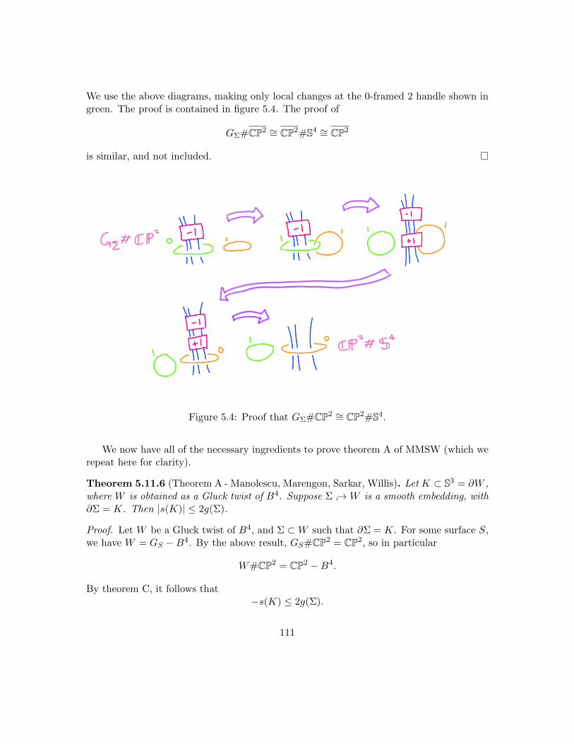
We use the above diagrams, making only local changes at the 0-framed 2 handle shown ingreen. The proof is contained in figure 5.4. The proof of
GΣ#CP2 ∼= CP2#S4 ∼= CP2
is similar, and not included.
Figure 5.4: Proof that GΣ#CP2 ∼= CP2#S4.
We now have all of the necessary ingredients to prove theorem A of MMSW (which werepeat here for clarity).
Theorem 5.11.6 (Theorem A - Manolescu, Marengon, Sarkar, Willis). Let K ⊂ S3 = ∂W ,where W is obtained as a Gluck twist of B4. Suppose Σ →W is a smooth embedding, with∂Σ = K. Then |s(K)| ≤ 2g(Σ).
Proof. Let W be a Gluck twist of B4, and Σ ⊂W such that ∂Σ = K. For some surface S,we have W = GS −B4. By the above result, GS#CP2 = CP2, so in particular
W#CP2 = CP2 −B4.
By theorem C, it follows that−s(K) ≤ 2g(Σ).
111
Moreover, we also know that GS#CP2 = CP2, from which it follows that W#CP2 =
CP2 −B4, so by theorem B,s(K) ≤ 2g(Σ).
Combining these two results, we find that
|s(K)| ≤ 2g(Σ)
as required.
Is there any hope for the FGMW strategy? A modification of the strategy which mightstill work is the following result:
Proposition 5.11.7. Suppose K,K ′ are knots with S30(K) ∼= S3
0(K ′), but with K sliceand K ′ not slice. Then SPC4 is false.
Proof. Recall that S30(K) denotes the result of 0-surgery on K. The above result follows
from the trace embedding lemma, which we saw in the previous lecture. Let X0(K) andX0(K ′) denote the traces of 0-surgery along K and K ′ respectively. Then ∂X0(K) =∂X0(K ′) as smooth manifolds. On one hand, we know that
S4 = X0(K) ∪ (B4 − nbhd(D)),
where the union glues along the boundary. Therefore we can replace X0(K) with X0(K ′),and consider
S′ = X0(K ′) ∪ (B4 − nbhd(D)).
From Mayer-Vietoris, Seifert-van Kampen, and the topological Poincare conjecture, onecan show that S′ is homeomorphic to S4. However, since K ′ is not slice, it cannot be dif-feomorphic to S4 (by the trace embedding lemma). Therefore S′ is an exotic S4, disprovingSPC4.
So far such K and K ′ have not been found, but there is also no evidence that theycannot be found!
5.12 Combinatorial proof of the Thom conjecture
In 2018, Lambert-Cole1 proved the Thom conjecture using Khovanov homology techniquesand no gauge theory. We give a very brief outline of the ingredients of the proof here. Butfirst - let us recall the statement of the Thom conjecture.
1Originally I had erroneously written Lambert and Cole instead of Lambert-Cole, thinking it was workby two authors. Lambert-Cole himself emailed me to correct my mistake:“Dear Mr Fushida
I came across your excellent lecture notes from Ciprian Manolescu’s 4-manifold class. However I noticedan error (see attached). I’m sure this is simply a miscommunication between yourself and Mr Hardy, butPeter Lambert-Cole is in fact a single person.
Best, Peter Lambert-Cole”
112

Theorem 5.12.1 (Thom conjecture). Let Σ ⊂ CP2 be a smoothly embedded connected(real) surface, and suppose [Σ] = d[CP1] ∈ H2(CP2;Z) ∼= Z. Then the genus of Σ isbounded below by (d− 1)(d− 2)/2.
To prove this theorem using Khovanov homology, we require three main ingredients, asfollows.
Trisections. Let Σ as in the proposition be given. We choose a trisection of CP2,forwhich Σ is in a “bridge” position. That is, it arches over the three components ofthe trisection. In particular, each Σ ∩ Yi (where Yi is an interface of the trisection)does not intersect either of the other two Yj .
Contact geometry. We make each Σ∩Yi transverse to the standard contact structurein #k(S1 × S2).
Khovanov homology. We use the slice-Bennequin inequality for transverse knots,which can be proved using Khovanov homology. (In fact, this is equivalent to Milnor’sconjecture!)
This completes the course! Thank you Ciprian for an amazing class.
113