Shelling (Bruggesser-Mani 1971) and Ranking

Let � � � � � � � � � � � � � � � � � � � � � � � be a polytope.� hassuch a representation iff it contains the origin in its interior. For a generic

� � � � , sort the inequalities so that � � � � � � � � � � � � � � � .

( � a ranking of vertices� ’s in the dual by a linear function).

Geometrically, the line� � � � � � � � � � � � � meets each hyperplane

� � � � . Let � denotes the parameter value at the intersection. Thus,� � � � and � � � � �

Consequently:

� � � � � � � � � � � � � � � � � � �

This ordering induces a shelling of� :

� � ! �

" � # � $ # is a topological� % & � � -ball for each

� ' � & � .

24

Shelling and Ranking (cont.)

F1

F3

F4

F2

0

c

F5

x

z1

z2

xz3

z4

z5

P

25

Shelling in � � (Launching a Space Shuttle)

z1

z3

z2

z4

z5

z12

z4

L

F4

(a)

(b)

26

Shelling in � � (cont.)

F1 F2

F3

F4

F5

F6

F7

F12F11

F10

F9

F8

27

The Double Description Method: Complexity?� : an H-polytope represented by� halfspaces� � , � � � , � � in � � .

� � $ " � � : ' th polytope (� � � � ).

� � � � � � : the vertex set computed at' th step.

(Pk-1, Vk-1) (Pk, Vk)

hk

newlygeneratedfor each adjpair ( , )

28

The Double Description Method: Complexity? (cont.)� It is anincremental method, dual to the Beneath-Beyond Method.

� Practical for low dimensions and highly degenerate inputs.

� For highly degenerate inputs, the sizes of intermediate polytopes are

very sensitive to the orderingof halfspaces. For example, the

maxcutoff ordering (“the deepest cut”) may provoke extremely high

intermediate sizes.

� It is hard to estimate its complexity in terms of and the sizesof input

and output. The main reason is that the intermediate polytopes �

can become very complex relative to the original polytope� � � � .

� D. Bremner (1999) proved that there is a class of polytopes for which

the double description method (and the beneath-beyond) method is

exponential.

29

How Intermediate Sizes Fluctuate with Different Orderings

20 22 24 26 28 30 32Iteration

250

500

750

1000

1250

1500

Size INTERMEDIATE SIZES FOR CCP6

maxcutoff

mincutoffrandom

lexmin

The input is a� � -dimensional polytope with� � facets. The output is a list

of � � � vertices. The lexmin is a sort of shelling ordering.

30

How Intermediate Sizes Fluctuate with Different Orderings

200 400 600 800 1000

5000

10000

15000

20000

25000

30000

Iteration

Size

Random

Maxcutoff

Mincutoff

The input is a� � -dimensional cross polytope with� � � facets. The output

is a list of � � vertices. The highest peak is attained by maxcutoff ordering,

following by random and mincutoff. Lexmin is the best among all and the

peak intermediate size is less than� � . (Too small too see it above.)

31

Pivoting Algorithms for Vertex Enumeration

Basic Idea:Search the connected graph of an H-polytope� by pivotingoperations to list all vertices.

A polytope � and its graph (1-skeleton)

Advantage:Under the usual nondegeneracy (i.e. no points in� lie onmore than% facets), it is polynomial in the input size and the output size.

Space Complexity:Depends on the search technique. The standarddepth-first search requires to store all vertices found.

32

Memory Free: Reverse Search for Vertex Enumeration

Key idea:Reverse the simplex method from theoptimal vertexin allpossible ways:

!!

!$

"*

#"

$"

min x1 + x2 + x3

Complexity: � � � % � � � -time and� � � % � -space (under nondegeneracy).

33

Reverse Search: General Description

Two functions� and � � � define the search:

A finite local search� for a graph� � � � � � � with a special node� � �

is a function: � � � � � � � satisfying

(L1) � � � � � � � � � � for each� � � � � � � , and

(L2) for each� � � � � � � , ' � � such that� � � � � � .

Example:

� Let � � � � � � � � � � � be a simple polytope, and�� � be any

generic linear objective function. Let� be the set of all vertices of

� , � the unique optimal, and� � � � be the vertex adjacent to� selected

by the (deterministic) simplex method.

34

Reverse Search: General Description

A adjacency oracle� � � for a graph� � � � � � � is a function (where� a

upper bound for the maximum degree of� ) satisfying:

(i) for each vertex� and each number' with � ' � the oracle returns

� � � � � � ' � , a vertex adjacent to� or extraneous� (zero),

(ii) if � � � � � � ' � � � � � � � � '�

� �� � for some� � � , ' and ' � , then ' � ' � ,

(iii) for each vertex� , � � � � � � � ' � � � � � � � � ' � �� � � � ' � � is exactly

the set of vertices adjacent to� .

Example:

� Let � � � � � � � � � � � be a simple polytope. Let� be the set

of all vertices of� , � be the number of nonbasic variables and

� � � � � � ' � be the vertex adjacent to� obtained by pivoting on the' th

nonbasic variable at� .

35

Reverse Search: General Description

procedure ReverseSearch(� � � , � , � , � );� � � � ; � � ; (* : neighbor counter *)

repeatwhile � � do

� � � ;

(r1) � � � � � � � � � � � � � ;

if � � � � �� then(r2) if � � � � � � �

� � then (* reverse traverse *)

� � � � � � � ; � � endif

endifendwhile;

if � �� � then (* forward traverse *)

(f1) � � � � ; � � � � � � � ;

(f2) � � ; repeat � � � until � � � � � � �� � (* restore *)

endifuntil � � � and � �

36

Pivoting Algorithm vs Incremental Algorithm� Pivoting algorithms, in particular the reverse search algorithm (lrs,

lrslib), work well for high dimensional cases.

� Incremental algorithms work well for low (up to� � ) dimensionalcases and highly degenerate cases. For example, the codes cdd/cddliband porta are implemented for highly degenerate cases and the codeqhull for low (up to � � ) dimensional cases.

� The reverse search algorithm seems to be the only method thatscalesvery efficiently in massively parallel environment.

� Various comparisons of representation conversion algorithms andimplementations can be found in the excellent article:

D. Avis, D. Bremner, and R. Seidel. How good are convex hullalgorithms.ComputationalGeometry:TheoryandApplications,7:265–302, 1997.

37

Voronoi Diagram in � �

� : a set of� distinct points in� �

Voronoi diagram is the partition of� � into � polyhedral regions:

� � � � � � � � � ��

� % � � � � � � � % � � � � � � � � � � � &� � � for � � �

where % � � is the Euclidean distance function. Each region� � � � � is called

theVoronoi cell of � .

38

Voronoi Diagram as Polyhedral Projection

For � in � , consider the hyperplane� � � � tangent to the paraboloid

( � � � � � � �� � � � � � � �� ) in �� � � at � :

�� " �

��

�&

�� " �

� � � � � � � � � � � � �

Replacing equation with inequality� for each� � � , we obtain the

polyhedron

� � � � � � � � � ��

� " ���

�&

�� " �

� � � � � � � � � � � � � � � � � � �

The key observation is that for two distinct points� and � , the intersection

of two hyperplanes� � � � and � � � � is in fact the equal separator hyperplane

of the two points.

39

Voronoi Diagram as Polyhedral Projection

The Voronoi diagram is simply the orthogonal projection of� � �� � �

onto the original space� � .

The projected vertices of� are called theVoronoi vertices.

40

Delaunay Triangulation in � �

For each point� � �� , thenearestneighborset � � � � � � of � is the set of

points� � � which are closest to� in Euclidean distance.

The convex hull� � � � � � � � � � � � of the nearest neighbor set of a Voronoi

vertex � is called theDelaunaycell of � . TheDelaunaytriangulation of�

is a partition of the convex hull� � � � � � � into the Delaunay cells of

Voronoi vertices. The one-to-one correspondence between the Voronoi

vertices and the Delaunay cells is duality that .

41

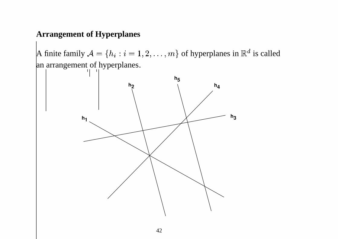
Arrangement of Hyperplanes

A finite family � � � � � � � � � � � � � � � � of hyperplanes in� � is calledanarrangementof hyperplanes.

h1

h2

h3

h4

h5

42

Arrangement of Hyperplanes: Representation of Faces��

� � � � � � � � � � � � � � � � � � � � �!

� � � � � � � � �

h1

h2

h3

h4

h5

+−

−

−++

_

+

_

+

(0-0-+)(+++++)

(++++0)

43

Central Arrangement of Hyperplanes

An arrangement of hyperplanes in which all its hyperplanes contain the

origin � is called acentralarrangementof hyperplanes.

h1

h2

h3

0

h4

+

-

- + +-

-

+

44

Central Arrangement and Sphere Arrangement

S1

S2

S4

S3

+

-

+ -

+

-

+-

(-+++)

(00++)

(-0++)

45

Polyhedral Realization of Arrangements

Let � be an arrangement of hyperplanes represented by a matrix� , i.e,

� � � � � � � � � � � � � � � � � � � � .

Consider the following polytope:� � � � � � �� � � � � � � � � & � � � � ��

�

Theorem 0.14. The face lattice of� is isomorphic to the face lattice ofthe polytope� � .

46

Dual of � � : A Zonotope

The polar of the polytope� � is the polytope (calledzonotope)

� � � �� � � � � � � �� � � � � � � � � & � � � � ��

�

� � �� � � � � � � � �& � � � � ��

�

� � � � � � � � � � � � � �

where eachgenerator� is the line segment� & � � � � .

(PA)*

47

Dual of � � : A Zonotope

The polar of the polytope� � is the polytope (calledzonotope)

� � � �� � � � � � � �� � � � � � � � � & � � � � ��

�

� � �� � � � � � � � �& � � � � ��

�

� � � � � � � � � � � � � �

where eachgenerator� is the line segment� & � � � � .

(PA)*

48

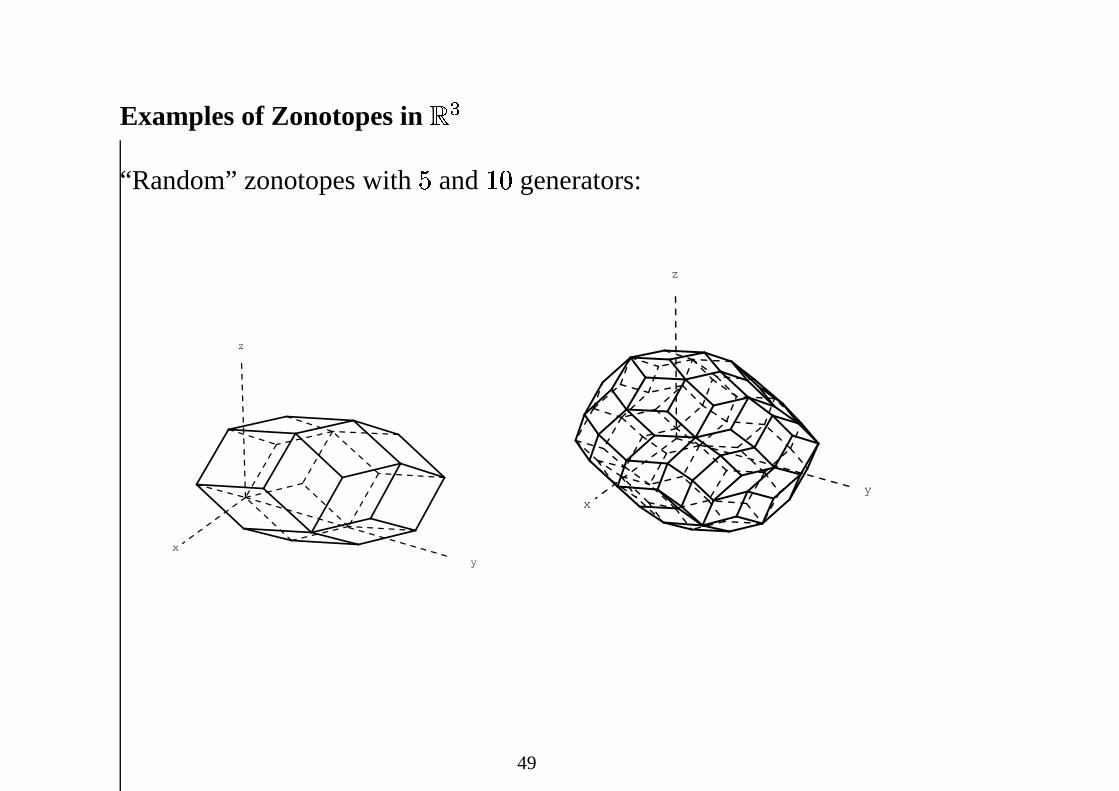
Examples of Zonotopes in � �

“Random” zonotopes with� and � � generators:

x

y

z

xy

z

49