Embed Size (px)
Citation preview
Traveling pulse emerges from individuals coordinating theirstop-and-go motion: a case study in sheep
Manon Azaıs1, Stephane Blanco2, Richard Bon1, Richard Fournier2, Marie-HelenePillot1, Jacques Gautrais1*
1 Centre de Recherches sur la Cognition Animale (CRCA), Centre de BiologieIntegrative (CBI), Universite de Toulouse; CNRS, UPS, France.2 LaPlaCE, Universite de Toulouse; CNRS, UPS, France.
Abstract
Monitoring small groups of sheep in spontaneous evolution in the field, we decipherbehavioural rules that sheep follow at the individual scale in order to sustain collectivemotion. Individuals alternate grazing mode at null speed and moving mode at walkingspeed, so cohesive motion stems from synchronising when they decide to switch betweenthe two modes. We propose a model for the individual decision making process, basedon switching rates between stopped / walking states that depend on behind / aheadlocations and states of the others. We parametrize this model from data. Next, wetranslate this (microscopic) individual-based model into its density-flow (macroscopic)equations counterpart. Numerical solving these equations display a traveling pulsepropagating at constant speed even though each individual is at any moment eitherstopped or walking. Considering the minimal model embedded in these equations, wederive analytically the steady shape of the pulse (sech square). The parameters of thepulse (shape and speed) are expressed as functions of individual parameters. This pulseemerges from the non linear coupling of start/stop individual decisions whichcompensate exactly for diffusion and promotes a steady ratio of walking / stoppedindividuals, which in turn determines the traveling speed of the pulse. The systemseems to converge to this pulse from any initial condition, and to recover the pulse afterperturbation. This gives a high robustness to this coordination mechanism.
Introduction
Behavioural mechanisms driving collective motion in animals and chemotactic bacteriahave raised a sustained interest over the last twenty years [Sumpter, 2006,Eftimie et al.,2007a,Tindall et al., 2008,Saragosti et al., 2010,Sumpter, 2010,Saragosti et al.,2011,Lopez et al., 2012,Vicsek and Zafeiris, 2012,Eftimie, 2012,Kuwayama and Ishida,2013,Carrillo et al., 2014,Pineda et al., 2015,Cavagna et al., 2016,Herbert-Read,2016,Jiang et al., 2017]. Beyond attraction/repulsion basics, lots of studies have beendevoted to understand how individuals coordinate their turns (velocity matching, inmagnitude and direction), either considering a constant speed module [Vicsek et al.,1995,Gautrais et al., 2012] or adaptive accelerations [Katz et al., 2011,Tunstrøm et al.,2013,Bialek et al., 2014]. Data-based models have been proposed to understand mutualinteractions within flocks and schools [Hemelrijk et al., 2015,Hemelrijk andHildenbrandt, 2015,Hemelrijk and Hildenbrandt, 2014,Gautrais et al., 2012,Ballerini
1
arX
iv:1
712.
0577
4v2
[nl
in.P
S] 6
Jul
201
8
et al., 2008a], and how they translate into large-scale correlations and informationpropagation at the group scale [Cavagna et al., 2016,Bialek et al., 2012,Attanasi et al.,2014,Attanasi et al., 2015,Calovi et al., 2015].
Here, we focus on a specific kind of speed coordination, namely for terrestrialanimals who display intermittent motion [Kramer and McLaughlin, 2001]: at any time,an individual is either stopped (null speed), or it is walking at a given constant speed.Such individual intermittent motion processes can combine into collective displays thatcould be poorly accounted for by continuous-speed models [Ginelli et al., 2015,Rimerand Ariel, 2017]. In a stop-go process, the behavioural decision is about the delay beforeswitching from stopped to walking, and back, depending on the relative position andmoving states of the others. In order to decipher the behavioural mechanisms at play sothat intermittent-moving animals keep moving together, we studied small groups ofsheep left alone grazing on their own on flat homogeneous pastures. Our purpose is firstto confirm that their decision making process in spontaneous condition in the field canbe modelled by extending a previous model that accounted for their decision makingprocess in manipulative condition. Our second purpose is to derive a macroscopic modelbased on this microscopic (individual) behavioral rules.
Biological background
We followed the spontaneous evolution of groups of N = 2, 3, 4, 8 Merino sheep,introduced in fence-delimited square pens (80 x 80 m) planted in flat irrigated pastures(groups of N = 100 sheep have also been monitored in the same series of experimentsand have been the subject of a separate study, reported in a previous paper [Ginelliet al., 2015]).
After habituation time, the groups adopted a collective behaviour alternating phasesof quasi-static grazing and phases of head-up walking (see Movie S1 for an illustrationwith a group of three sheep). There was a striking coordination of these phases amongindividuals, so that, most of time, a group is either found with all individuals grazing orall individuals walking. The collective grazing phases are characterised by individualshardly moving and keeping very close to each others (within the meter). The collectivewalking phases are much shorter than grazing phases and can translocate the groupsover several tens of meters.
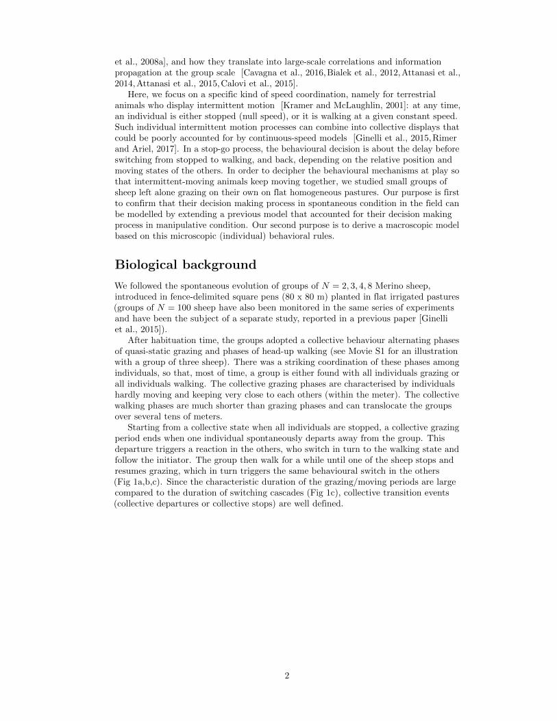
Starting from a collective state when all individuals are stopped, a collective grazingperiod ends when one individual spontaneously departs away from the group. Thisdeparture triggers a reaction in the others, who switch in turn to the walking state andfollow the initiator. The group then walk for a while until one of the sheep stops andresumes grazing, which in turn triggers the same behavioural switch in the others(Fig 1a,b,c). Since the characteristic duration of the grazing/moving periods are largecompared to the duration of switching cascades (Fig 1c), collective transition events(collective departures or collective stops) are well defined.
2
0 −10 −20 −30 −40 −50 −60
0
5
10
15
20
25
30
35
X (m)
Y (
m)
Grazing
Grazing
Walking
a
0 −10 −20 −30 −40 −50 −60
0
5
10
15
20
25
30
35
X (m)
Y (
m)
b
740 760 780 800
Time (s)
Nu
mb
er
wa
lkin
g
0
1
2
3
Starts Stops
Grazing Walking Grazing
c
0 500 1000 1500
0
50
100
150
200
Time (s)
S (
m)
d
Fig 1. Coordination of motion illustrated in one experimental group of 3sheep. The position and behaviour of each individual is monitored every 1s during1800 s. The collective behaviour can be categorised as periods of collective grazing(individuals are about motionless) interspersed by periods of collective walking (highspeed motion). (a) An extract of 70 s shows a typical event of collective transition fromgrazing to walking, leading to a spatial shift of the group to a new location whereindividuals resume grazing. (b) The data are idealised by binarizing individual speed(0,1) and the motion is projected in 1D along the axis of collective motion. (c) Thesame event reported in time shows that the collective starts and stops are triggered bysheep synchronising their transition from grazing to walking (and back) within timewindows by far shorter than typical duration of grazing / walking periods. (d)Time-space representation of group evolution in 1D. Alternating synchronouslygrazing/walking/grazing over large time (1800 s) lead to a collective stop-and-goprogression along the curvilinear abscissa S of the group trajectory. The extracted eventof 70 s is highlighted.
3
Regarding the directional process, we observed that the followers always adopted abearing matching the initiator’s (they followed him, Fig 1a), so that we will not addresshere the orientational decision, taking for granted that the initiator chooses a bearing,that the followers will systematically mimic. We can thus consider the spatial progressof a group along the multi-segments trajectory of the group center of mass, indexing theindividual positions by projecting their 2D positions onto the corresponding curvilinearabscissa along this group trajectory (Fig 1b). Doing this, the collective dynamics areidealised as individuals progressing in 1D towards positive abscissa (Fig 1d), and thequestion becomes to understand the mechanisms synchronising their switches fromnull-speed grazing to full-speed progression, and back (Fig 1c).
In previous studies, we have proposed an individual-based model to explain thecollective dynamics of group departures [Petit et al., 2009,Pillot et al., 2011], andgroup stops [Toulet et al., 2015] observed in a manipulative setup, using a remotecontrol device to trigger the departure of a first (trained) individual [Pillot et al.,2011,Toulet et al., 2015]. In this model, individuals are in two possible states: stoppedor moving (at speed v). Their transitions from state to state are governed by atransition rate (probability switching state per unit time), which depends on the stateconfiguration of the others. In [Pillot et al., 2011], we only considered collectivedepartures of naive individuals after the trained individual had departed. We had founda double mimetic effect based on the state of the others: departed individuals tend tostimulate stopped individuals to switch to moving while still stopped individuals tendsto inhibit it. The higher the number of individuals that have already departed, thehigher the rate to depart. The higher the number of individuals that are still stopped,the lower the rate to depart. We proposed then a formal dependence of thestopped-to-moving (activation) switching rate K
A, following:
KA
(A, I) = αAβ
Iγ(1)
where A denotes the number of moving individuals (departed, active) and I thenumber of stopped individuals (not departed, inactive). We checked in a later study[Toulet et al., 2015] that the same double mimetic effect can explain as well howmoving-to-stopped (inactivation) switchings escalate in a group of moving individuals toreach a consensus to stop.
In those previous studies, only one event (collective departure or collective stop) wasmonitored at a time, a trained individual was used to trigger the collective events andthe model was purely temporal. To give account of groups behaviour in the presentstudy, we start from the same model, to which we add two ingredients so that groupscan chain multiple collective departures / collective stops as they meanderspontaneously on the pasture.
The first ingredient accounts for the spontaneous switching rates, to allow a firstindividual to depart from a stopped group and a first individual to stop in a movinggroup.
A second ingredient is needed to introduce spatial effects. In the present setup(small groups on open pastures), it was obvious that each sheep can monitor every otherone, so we do not introduce limited range of interaction (this point is discussed furtherin the Discussion), neither metric nor topologic [Ballerini et al., 2008a]. As a proxy forthe relevant information in sheep decisions, we consider only relative positions along the1-dimensional group trajectory, so that one individual can make a difference betweenindividuals ahead of him and individuals behind him. The states configuration of theothers around can then be split into four pools: the individuals behind him that arestopped I−, the ones behind him that are moving A−, the ones ahead that are stoppedI+ and the ones ahead that are moving A+.
4
For the stopped-to-moving switching rates KA
(activation), the double mimeticeffects become:
KA
(A−, I−, A+, I+) = µA
+ αA
[A+]βA
[A−+I−+I+]γA
= µA
+ αA
[A+]βA
[N−A+]γA
(2)
and for the moving-to-stopped switching rates:
KI(A−, I−, A+, I+) = µ
I+ α
I
[I−]βI
[A++A−+I+]γI
= µI
+ αI
[I−]βI
[N−I−]γI
(3)
where we have considered that only neighbours ahead and moving, A+, arestimulating switches to motion (the others inhibiting it) and only stopped neighboursbehind, I−, are stimulating stopping decision of a moving animal (the others inhibitingit). This modeling choice is discussed further in the Discussion. In absence ofstimulating individuals, the rates reduce to the spontaneous switching rates µ
Aand µ
I.
Parameters estimation
In order to estimate the parameters for the stimulated part (α•, β•, γ•), we collected allcollective transition events from 1800-s movie sequences, combining group sizes todisentangle the two mimetic effects, as in [Pillot et al., 2011,Toulet et al., 2015](Table 1).
Table 1. Individual parameters for the double mimetic effect.
Parameter Stopped-to-Moving Kept Moving-to-Stopped Kept
α (s−1) 0.32 [0.25;0.41] 0.3 0.42 [0.33;0.54] 0.4β 0.61 [0.44;0.78] 0.6 0.48 [0.31;0.65] 0.5γ 0.71 [0.53;0.87] 0.7 0.54 [0.36;0.71] 0.5
Table notes Mean estimates and 95% CI are given for each parameter and for bothkinds of transition. In Kept columns are reported the mean estimates rounded at thefirst decimal, which was retained in the model.
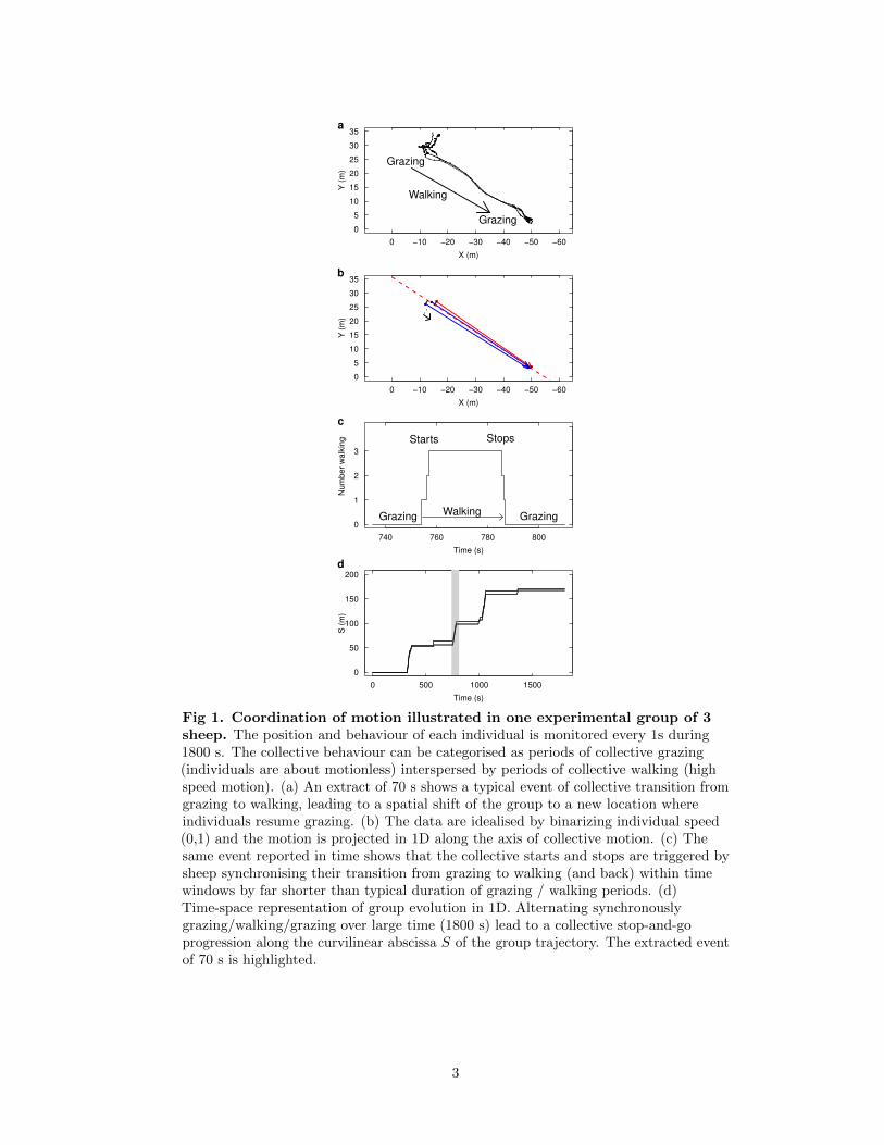
This functional dependence fitted with the experimental rates as nicely as in ourprevious studies (Fig 2a,c), and correctly predicted as well the duration of eventsdepending on group size (Fig 2b,d).
The spontaneous rate of switching to the stopped state µI was straightforwardlyretrieved from collective moves duration, and we found that it depends on the groupsize N , following:
µI = µ∗I/N (4)
with µ∗I = 0.08 s−1.The spontaneous rate of switching to the walking state was practically impossible to
estimate from data because small grazing moves and actual departures as an initiatorwere too difficult to discriminate. A reasonable estimate is however µA = 0.0055 (s−1),corresponding to a mean time of 3 minutes before next spontaneous departure. This
5
0.0
0.2
0.4
0.6
0.8
1.0
Nb. Walking
Depart
ing r
ate
(s
−1)
1 1 2 1 2 3 1 2 3 4 5 6 7
a
0
2
4
6
8
10
12
Group Size
Eve
nt D
ura
tion (
s)
2 3 4 8
b
0.0
0.2
0.4
0.6
0.8
1.0
Nb. Stopped
Sto
ppin
g r
ate
(s
−1)
1 1 2 1 2 3 1 2 3 4 5 6 7
c
0
2
4
6
8
10
12
Group Size
Eve
nt D
ura
tion (
s)
2 3 4 8
d
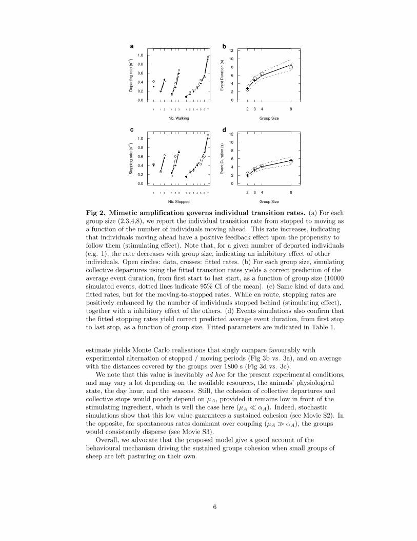
Fig 2. Mimetic amplification governs individual transition rates. (a) For eachgroup size (2,3,4,8), we report the individual transition rate from stopped to moving asa function of the number of individuals moving ahead. This rate increases, indicatingthat individuals moving ahead have a positive feedback effect upon the propensity tofollow them (stimulating effect). Note that, for a given number of departed individuals(e.g. 1), the rate decreases with group size, indicating an inhibitory effect of otherindividuals. Open circles: data, crosses: fitted rates. (b) For each group size, simulatingcollective departures using the fitted transition rates yields a correct prediction of theaverage event duration, from first start to last start, as a function of group size (10000simulated events, dotted lines indicate 95% CI of the mean). (c) Same kind of data andfitted rates, but for the moving-to-stopped rates. While en route, stopping rates arepositively enhanced by the number of individuals stopped behind (stimulating effect),together with a inhibitory effect of the others. (d) Events simulations also confirm thatthe fitted stopping rates yield correct predicted average event duration, from first stopto last stop, as a function of group size. Fitted parameters are indicated in Table 1.
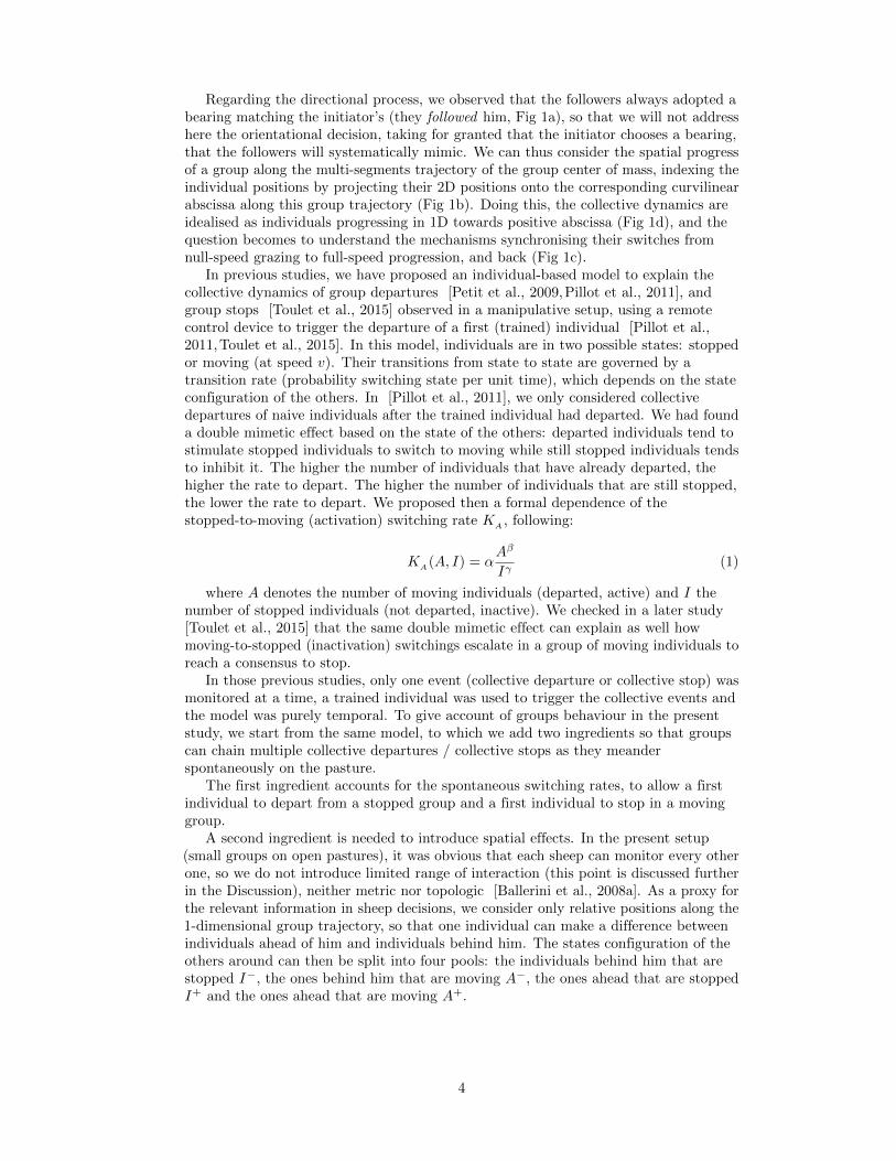
estimate yields Monte Carlo realisations that singly compare favourably withexperimental alternation of stopped / moving periods (Fig 3b vs. 3a), and on averagewith the distances covered by the groups over 1800 s (Fig 3d vs. 3c).
We note that this value is inevitably ad hoc for the present experimental conditions,and may vary a lot depending on the available resources, the animals’ physiologicalstate, the day hour, and the seasons. Still, the cohesion of collective departures andcollective stops would poorly depend on µA, provided it remains low in front of thestimulating ingredient, which is well the case here (µA � αA). Indeed, stochasticsimulations show that this low value guarantees a sustained cohesion (see Movie S2). Inthe opposite, for spontaneous rates dominant over coupling (µA � αA), the groupswould consistently disperse (see Movie S3).
Overall, we advocate that the proposed model give a good account of thebehavioural mechanism driving the sustained groups cohesion when small groups ofsheep are left pasturing on their own.
6
0 500 1000 1500
0
20
40
60
80
100
120
Time (s)
S (
m)
Dataa
0 500 1000 1500
0
20
40
60
80
100
120
Time (s)
S (
m)
Modelb
0 500 1000 1500
0
20
40
60
80
100
120
Dis
tan
ce
wa
lke
d (
m)
c
0 500 1000 1500
0
20
40
60
80
100
120
Dis
tan
ce
wa
lke
d (
m)
d
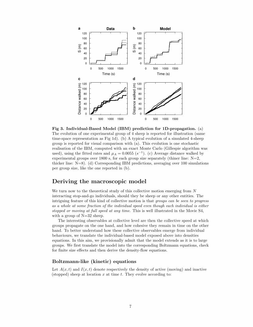
Fig 3. Individual-Based Model (IBM) prediction for 1D-propagation. (a)The evolution of one experimental group of 4 sheep is reported for illustration (sametime-space representation as Fig 1d). (b) A typical evolution of a simulated 4-sheepgroup is reported for visual comparison with (a). This evolution is one stochasticrealisation of the IBM, computed with an exact Monte Carlo (Gillespie algorithm wasused), using the fitted rates and µA = 0.0055 (s−1). (c) Average distance walked byexperimental groups over 1800 s, for each group size separately (thiner line: N=2,thicker line: N=8). (d) Corresponding IBM predictions, averaging over 100 simulationsper group size, like the one reported in (b).
Deriving the macroscopic model
We turn now to the theoretical study of this collective motion emerging from Ninteracting stop-and-go individuals, should they be sheep or any other entities. Theintriguing feature of this kind of collective motion is that groups can be seen to progressas a whole at some fraction of the individual speed even though each individual is eitherstopped or moving at full speed at any time. This is well illustrated in the Movie S4,with a group of N=32 sheep.
The interesting observables at collective level are then the collective speed at whichgroups propagate on the one hand, and how cohesive they remain in time on the otherhand. To better understand how these collective observables emerge from individualbehaviours, we translate the individual-based model exposed above into densitiesequations. In this aim, we provisionally admit that the model extends as it is to largegroups. We first translate the model into the corresponding Boltzmann equations, checkfor finite size effects and then derive the density-flow equations.
Boltzmann-like (kinetic) equations
Let A(x, t) and I(x, t) denote respectively the density of active (moving) and inactive(stopped) sheep at location x at time t. They evolve according to:
7
{∂tI(x, t) = −KA(x, t)I(x, t) +KI(x, t)A(x, t)
∂tA(x, t) + v∂xA(x, t) = +KA(x, t)I(x, t)−KI(x, t)A(x, t)(5)
where KA(x, t) and KI(x, t) are respectively the conversion rates fromstopped-to-moving (activation) and moving-to-stopped (inactivation) at location x attime t, which depend on A and I according to:
KA(x, t) = µA
+αA
[∫∞xA(u, t)du
]βA[N −
∫∞xA(u, t)du
]−γAKI(x, t) = µ
I+α
I
[∫ x−∞ I(u, t)du
]βI[N −
∫ x−∞ I(u, t)du
]−γI (6)
with N =∫∞−∞A(u, t) + I(u, t)du is the total amount of sheep (which is conserved in
time), and parameters are those given in the individual-based model. This descriptionin density is the direct translation of the individual model expressions (in the limit ofcontinuum theory).
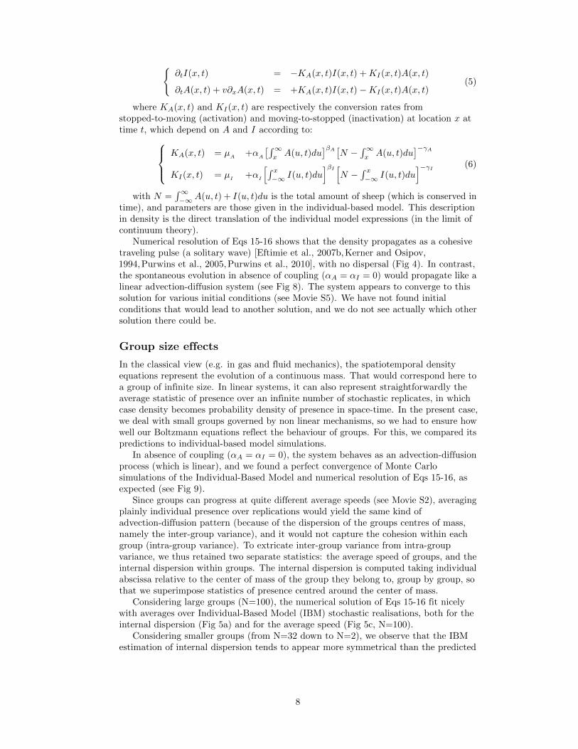
Numerical resolution of Eqs 15-16 shows that the density propagates as a cohesivetraveling pulse (a solitary wave) [Eftimie et al., 2007b,Kerner and Osipov,1994,Purwins et al., 2005,Purwins et al., 2010], with no dispersal (Fig 4). In contrast,the spontaneous evolution in absence of coupling (αA = αI = 0) would propagate like alinear advection-diffusion system (see Fig 8). The system appears to converge to thissolution for various initial conditions (see Movie S5). We have not found initialconditions that would lead to another solution, and we do not see actually which othersolution there could be.
Group size effects
In the classical view (e.g. in gas and fluid mechanics), the spatiotemporal densityequations represent the evolution of a continuous mass. That would correspond here toa group of infinite size. In linear systems, it can also represent straightforwardly theaverage statistic of presence over an infinite number of stochastic replicates, in whichcase density becomes probability density of presence in space-time. In the present case,we deal with small groups governed by non linear mechanisms, so we had to ensure howwell our Boltzmann equations reflect the behaviour of groups. For this, we compared itspredictions to individual-based model simulations.
In absence of coupling (αA = αI = 0), the system behaves as an advection-diffusionprocess (which is linear), and we found a perfect convergence of Monte Carlosimulations of the Individual-Based Model and numerical resolution of Eqs 15-16, asexpected (see Fig 9).
Since groups can progress at quite different average speeds (see Movie S2), averagingplainly individual presence over replications would yield the same kind ofadvection-diffusion pattern (because of the dispersion of the groups centres of mass,namely the inter-group variance), and it would not capture the cohesion within eachgroup (intra-group variance). To extricate inter-group variance from intra-groupvariance, we thus retained two separate statistics: the average speed of groups, and theinternal dispersion within groups. The internal dispersion is computed taking individualabscissa relative to the center of mass of the group they belong to, group by group, sothat we superimpose statistics of presence centred around the center of mass.
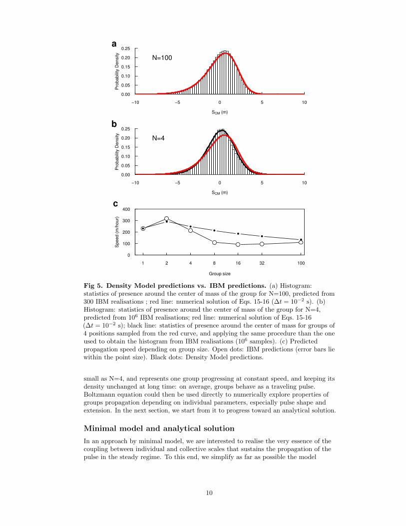
Considering large groups (N=100), the numerical solution of Eqs 15-16 fit nicelywith averages over Individual-Based Model (IBM) stochastic realisations, both for theinternal dispersion (Fig 5a) and for the average speed (Fig 5c, N=100).
Considering smaller groups (from N=32 down to N=2), we observe that the IBMestimation of internal dispersion tends to appear more symmetrical than the predicted
8
0 50 100 150 200
0.0
0.2
0.4
0.6
0.8
space (m)
density (
sheep/m
)
a
−10 −5 0 5 10
0.0
0.2
0.4
0.6
0.8
SCM (m)
Density
b
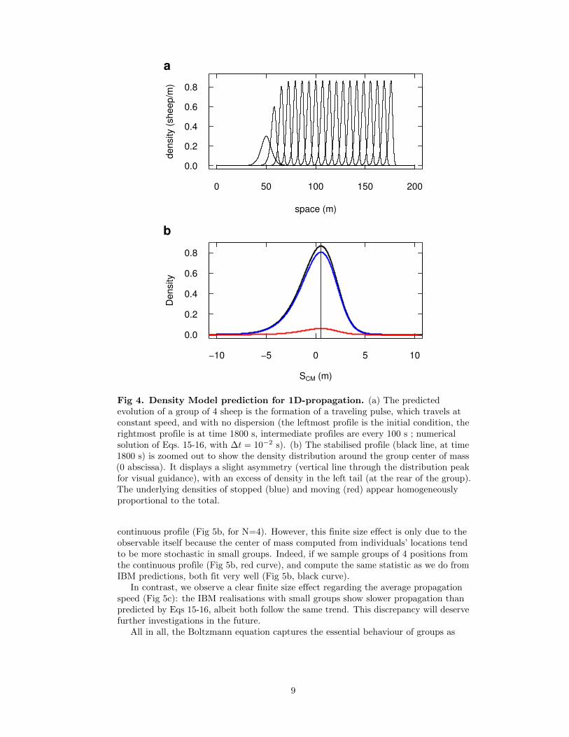
Fig 4. Density Model prediction for 1D-propagation. (a) The predictedevolution of a group of 4 sheep is the formation of a traveling pulse, which travels atconstant speed, and with no dispersion (the leftmost profile is the initial condition, therightmost profile is at time 1800 s, intermediate profiles are every 100 s ; numericalsolution of Eqs. 15-16, with ∆t = 10−2 s). (b) The stabilised profile (black line, at time1800 s) is zoomed out to show the density distribution around the group center of mass(0 abscissa). It displays a slight asymmetry (vertical line through the distribution peakfor visual guidance), with an excess of density in the left tail (at the rear of the group).The underlying densities of stopped (blue) and moving (red) appear homogeneouslyproportional to the total.
continuous profile (Fig 5b, for N=4). However, this finite size effect is only due to theobservable itself because the center of mass computed from individuals’ locations tendto be more stochastic in small groups. Indeed, if we sample groups of 4 positions fromthe continuous profile (Fig 5b, red curve), and compute the same statistic as we do fromIBM predictions, both fit very well (Fig 5b, black curve).
In contrast, we observe a clear finite size effect regarding the average propagationspeed (Fig 5c): the IBM realisations with small groups show slower propagation thanpredicted by Eqs 15-16, albeit both follow the same trend. This discrepancy will deservefurther investigations in the future.
All in all, the Boltzmann equation captures the essential behaviour of groups as
9
SCM (m)P
rob
ab
ility
De
nsity
−10 −5 0 5 10
0.00
0.05
0.10
0.15
0.20
0.25
N=100
a
SCM (m)
Pro
ba
bili
ty D
en
sity
−10 −5 0 5 10
0.00
0.05
0.10
0.15
0.20
0.25
N=4
b
0
100
200
300
400
Group size
Sp
ee
d (
m/h
ou
r)
1 2 4 8 16 32 100
c
Fig 5. Density Model predictions vs. IBM predictions. (a) Histogram:statistics of presence around the center of mass of the group for N=100, predicted from300 IBM realisations ; red line: numerical solution of Eqs. 15-16 (∆t = 10−2 s). (b)Histogram: statistics of presence around the center of mass of the group for N=4,predicted from 106 IBM realisations; red line: numerical solution of Eqs. 15-16(∆t = 10−2 s); black line: statistics of presence around the center of mass for groups of4 positions sampled from the red curve, and applying the same procedure than the oneused to obtain the histogram from IBM realisations (106 samples). (c) Predictedpropagation speed depending on group size. Open dots: IBM predictions (error bars liewithin the point size). Black dots: Density Model predictions.
small as N=4, and represents one group progressing at constant speed, and keeping itsdensity unchanged at long time: on average, groups behave as a traveling pulse.Boltzmann equation could then be used directly to numerically explore properties ofgroups propagation depending on individual parameters, especially pulse shape andextension. In the next section, we start from it to progress toward an analytical solution.
Minimal model and analytical solution
In an approach by minimal model, we are interested to realise the very essence of thecoupling between individual and collective scales that sustains the propagation of thepulse in the steady regime. To this end, we simplify as far as possible the model
10
presented above by setting βA = βI = 1, and neglecting inhibitory effects: γA = γI = 0.Doing this, we keep only the two essential components: the spontaneous switch of speed(driven by µA and µI), and the stimulating effect of the others (driven by αA and αI).
To derive an analytical solution, we first translate the Boltzmann equations aboveinto the corresponding “macroscopic” density-flow equations. We selected eventuallytwo variables to describe this evolution. The dispersion can be described by the sumdensity of sheep η(x, t) (moving and stopped) at location x at time t:
η(x, t) = A(x, t) + I(x, t) (7)
and the collective speed can be described by the moving fraction β(x, t) at location xat time t:
β(x, t) =A(x, t)
A(x, t) + I(x, t)=A(x, t)
η(x, t)(8)
the collective speed being v β(x, t), where v is the speed at which a walkingindividual walks.
Next we consider the traveling pulse at the steady regime, and write the equationgoverning its density profile n(y) in a moving frame anchored to the pulse peak (yindexing abscissa in the moving frame). This profile obeys:
(n′)2 − nn′′ − αA + αIv
n3 = 0 (9)
where prime denotes regular derivative with respect to y.A solution to Eq.43 is given by:
n(y) =1
2Nγsech2 (γy) with γ =
N(αA + αI)
4v(10)
Full details for the analytical solution in the steady regime for the minimal model aregiven in Appendix 1 : Analytical solution in the steady regime for the minimal model.
This solution well recovers the numerical predictions of the Boltzmann expressionEqs 15-16, for different parameters α• (see see Movie S6 in which we have superimposedthis analytical solution in red upon the numerical prediction in black).
The full expression for the pulse profile in the field frame and the associatedpropagation speed are:
ηs(x, t) = N
2N(αA+αI)
4v sech2(
N(αA+αI)4v (x− b∗svt)
)βs(x, t) = b∗s =
(N2 (αA−αI)−µA−µI)+√
(N2 (αA−αI)−µA−µI)2+4µA
N2 (αA−αI)
N(αA−αI)
(11)
when αA 6= αI .In the symmetrical case where αA = αI , the steady state solution simplifies to:{
ηs(x, t) = N2Nα2v sech2(Nα2v (x− b∗svt))
βs(x, t) = b∗s = µA/(µA + µI)(12)
The shape of the pulse depends on individual speed v, reaction terms αA and αI andgroup size N , while the propagation speed of the pulse also depends on the spontaneousswitching rates µA and µI . Sensitivity of the latter to some parameters is illustrated innext section.
11
Sensitivity of the moving fraction to parameters
The collective behaviour of first interest is the mean speed at which groups propagate,and it is a direct reflect of the moving fraction, given by Eq 11. In the general case, thismoving fraction depends upon two kinds of parameters:
1. The rates of spontaneous switching µA and µI : in terms of individual behaviour,these rates govern the propensity for an individual to be the first to depart from astopped group, respectively the propensity for an individual to be the first to stopin a moving group.
2. The imitation rates αA and αI : in terms of individual behaviour, these ratesgovern the propensity for a stopped individual to imitate departing individuals,respectively the propensity for a moving individual to imitate stopping individuals.
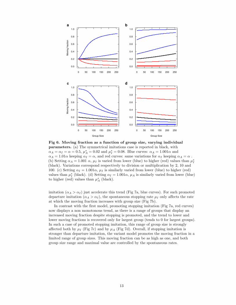
Fig 6 reports the moving fraction as a function of group size, varying the parameters.As mentioned above, in the case of symmetrical imitations, the moving fraction b∗s
appears to depend only on the rates of spontaneous switching µA and µI and in thisparticular case, it would not depend on the group size N (Fig 6a, black curve). In theasymmetric cases, the moving fraction also depends on imitation rates and on groupsize. Promoting departure imitation over stopping imitation (αA > αI), even by theslightest amount (Fig 6a, blue curves, αA = 1.001 αI and αA = 1.01 αI) lead largergroups to display higher and higher moving fractions (tends to 1 for large groups).Conversely, promoting stopping imitation (Fig 6a, red curves) lead larger groups tolower and lower moving fractions (tends to 0 for large groups).
The trend to full moving fractions for promoted departure imitation depends on thespontaneous stopping rate µI (Fig 6b). For very large values of µI (low moving fraction,Fig 6b, red curves), this trend is very slow and might be negligible. At the other end ofthe scope, very low µI values would promote a high moving fraction even for smallestgroup (Fig 6b, blue curves) so that the trend is also saturated. In between, µI has asensible effect upon the trend. The trend to null moving fractions for promotedstopping imitation is more affected by µI (Fig 6c) than by µA (Fig 6d), especially whenit is low (Fig 6c, blue curves).
Overall, the moving fraction depending on group size is especially sensitive to slightpromotion of imitation rates, but also to spontaneous stopping rate when the latter islow.
As a variant of the model, our data suggest that the spontaneous stopping rate isregulated by the group size N (Eq.4) such that walking individuals in large groups tendto spontaneously stop less often. In such a case, the moving fraction in the symmetricalimitation case, should be rewritten as:
b∗s =µA
µA + (µI/N)(13)
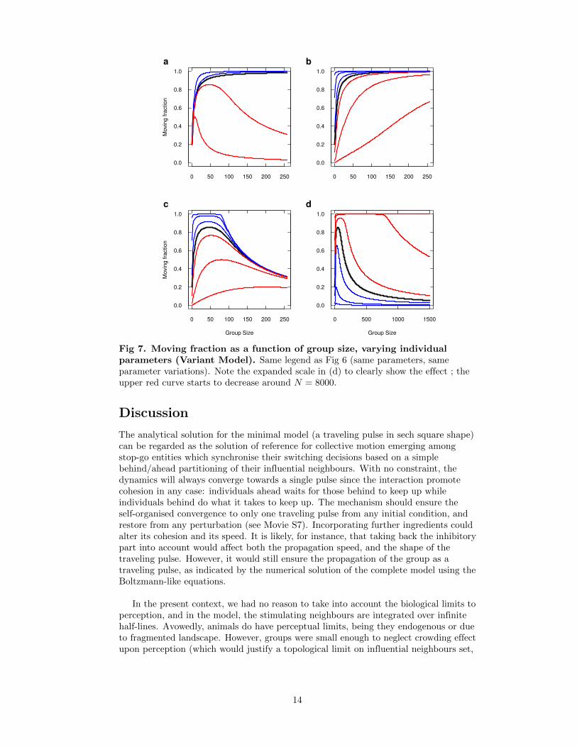
Avowedly, extending this property to very large groups would result in a vanishingspontaneous stopping rate, so that the moving fraction should tend to 1 in any case atfirst sight. This is actually true only in the symmetrical case. In the general case, thiseffect combines with other parameters and yields non monotonous trends with groupsize, so we expose it for the sake of interest. Fig 7 reports the moving fraction as afunction of group size (or total mass), varying the parameters the very same way as inFig. 6, but for the variant model (graphics can be compared one to one).
Introducing the variant produces a striking effect upon the sensitivity to parameters.First, as expected, the moving fraction increases with group size under the symmetricalinfluences case (Fig 7a, black curve). Promoting departure imitation over stopping
12
0 50 100 150 200 250
0.0
0.2
0.4
0.6
0.8
1.0
Movin
g fra
ction
a
0 50 100 150 200 250
0.0
0.2
0.4
0.6
0.8
1.0
b
0 50 100 150 200 250
0.0
0.2
0.4
0.6
0.8
1.0
Group Size
Movin
g fra
ction
c
0 50 100 150 200 250
0.0
0.2
0.4
0.6
0.8
1.0
Group Size
d
Fig 6. Moving fraction as a function of group size, varying individualparameters. (a) The symmetrical imitations case is reported in black, withαA = αI = α = 0.5, µ∗A = 0.02 and µ∗I = 0.08. Blue curves: αA = 1.001α andαA = 1.01α keeping αI = α, and red curves: same variations for αI keeping αA = α .(b) Setting αA = 1.001 α, µI is varied from lower (blue) to higher (red) values than µ∗I(black). Variations correspond respectively to division or multiplication by 2, 10 and100. (c) Setting αI = 1.001α, µI is similarly varied from lower (blue) to higher (red)values than µ∗I (black). (d) Setting αI = 1.001α, µA is similarly varied from lower (blue)to higher (red) values than µ∗A (black).
imitation (αA > αI) just accelerate this trend (Fig 7a, blue curves). For such promoteddeparture imitation (αA > αI), the spontaneous stopping rate µI only affects the rateat which the moving fraction increases with group size (Fig 7b).
In contrast with the first model, promoting stopping imitation (Fig 7a, red curves)now displays a non monotonous trend, as there is a range of groups that display anincreased moving fraction despite stopping is promoted, and the trend to lower andlower moving fractions is recovered only for largest group (tends to 0 for largest groups).In such a case of promoted stopping imitation, this range of group size is stronglyaffected both by µI (Fig 7c) and by µA (Fig 7d). Overall, if stopping imitation isstronger than departure imitation, the variant model promotes the moving fraction in alimited range of group sizes. This moving fraction can be as high as one, and bothgroup size range and maximal value are controlled by the spontaneous rates.
13
0 50 100 150 200 250
0.0
0.2
0.4
0.6
0.8
1.0
Movin
g fra
ction
a
0 50 100 150 200 250
0.0
0.2
0.4
0.6
0.8
1.0
b
0 50 100 150 200 250
0.0
0.2
0.4
0.6
0.8
1.0
Group Size
Movin
g fra
ction
c
0 500 1000 1500
0.0
0.2
0.4
0.6
0.8
1.0
Group Size
d
Fig 7. Moving fraction as a function of group size, varying individualparameters (Variant Model). Same legend as Fig 6 (same parameters, sameparameter variations). Note the expanded scale in (d) to clearly show the effect ; theupper red curve starts to decrease around N = 8000.
Discussion
The analytical solution for the minimal model (a traveling pulse in sech square shape)can be regarded as the solution of reference for collective motion emerging amongstop-go entities which synchronise their switching decisions based on a simplebehind/ahead partitioning of their influential neighbours. With no constraint, thedynamics will always converge towards a single pulse since the interaction promotecohesion in any case: individuals ahead waits for those behind to keep up whileindividuals behind do what it takes to keep up. The mechanism should ensure theself-organised convergence to only one traveling pulse from any initial condition, andrestore from any perturbation (see Movie S7). Incorporating further ingredients couldalter its cohesion and its speed. It is likely, for instance, that taking back the inhibitorypart into account would affect both the propagation speed, and the shape of thetraveling pulse. However, it would still ensure the propagation of the group as atraveling pulse, as indicated by the numerical solution of the complete model using theBoltzmann-like equations.
In the present context, we had no reason to take into account the biological limits toperception, and in the model, the stimulating neighbours are integrated over infinitehalf-lines. Avowedly, animals do have perceptual limits, being they endogenous or dueto fragmented landscape. However, groups were small enough to neglect crowding effectupon perception (which would justify a topological limit on influential neighbours set,
14
like in starling flocks or large fish flocks [Ballerini et al., 2008a,Rosenthal et al., 2015]),and landscape obstacles to perception would need to be introduced explicitly if theywere of relevance. Moreover, the dynamics favours packing against diffusion, so if smallgroups start from reasonably dense initial condition, the probability that the groupdisperse so widely that individuals could not see each other anymore due to endogenouslimit is nearly zero. In absence of external factors disrupting the groups, introducing abiologically relevant metric cutoff (e.g. some hundreds of meters in sheep) would thenhave no effect upon the sustained dynamics of the pulse (which is far narrower thanthat).
With no limited perception, the spatial effect results entirely from the asymmetricalinfluence of individuals that are in the opposite state: only active individuals ahead arestimulating switching to motion, only inactive individuals behind are stimulatingswitching to stop. The simple behind/ahead asymmetrical influence together with thedouble mimetic effect are sufficient to generate the traveling pulse since it promotes thetendency to wait at the front edge of the pulse, and to keep moving at the backedge [Mogilner and Edelstein-Keshet, 1999].
Without this simple asymmetry, e.g. if we had considered all (behind and ahead)active individuals as stimulating switching to motion, there would be no spatial effect atall, since the stimulation would be the same all over the space. In such a case, thedynamics would degenerate into a simple advection-diffusion process, and the groupwould eventually disperse despite interactions. This asymmetry can then be seen as analternative to models based upon topologically-defined neighbours [Ballerini et al.,2008b] or limited sensing kernels (non local terms) [Eftimie et al., 2007a]. It could aswell be described by an Heaviside odd kernels on the half-line. Considering extension to2-dimensional motion, our simple behind/ahead symmetry breaking parallels theviolation of Newton’s third law (action-reaction symmetry) in models based on socialforces [Barberis and Peruani, 2016].
Classically, traveling pulse studies start directly from a macroscopic description atthe system level [Kerner and Osipov, 1994,Purwins et al., 2005,Purwins et al., 2010]. Inthe present study, we have found a traveling pulse solution starting from the“microscopic” description of interactions at the individual level (and even binaryinteractions in the minimal model) so that the macroscopic solution (in the minimalversion of the model) is completely parametrized by the individual behavioralparameters.
In the same spirit, Bertin et al. [Bertin et al., 2009], extended by Peshkov etal. [Peshkov et al., 2014], propose a method to derive density equations for the Vicsekmodel [Vicsek et al., 1995] in the dilute regime (binary interactions). Starting from theBoltzmann expression (and using an approximation needed by the 2-dimensional natureof their model), they find an explicit expression of the macroscopic transportcoefficients. Projecting their Boltzmann expression onto an arbitrary direction in theunstable collective motion regime, the resulting 1-dimensional system display irregulartrains of traveling pulses. In contrast to the sech2 profile we found for our model, thesetraveling pulses profiles are made of two (behind / ahead) exponential decayscompatible with their hydrodynamic approximation. Saragosti et al. [Saragosti et al.,2010] also found double exponential wave profiles by deriving analytical macroscopicbehavior from a kinetic description of the mesoscopic run-and-tumble process inchemotactic bacteria E. coli. Such traveling bands have been long identified inlarge-scale IBM simulations [Chate et al., 2008,Ginelli et al., 2010]. The Vicsek modelassuming a constant velocity module, it would be interesting to study the effect ofincorporating coupled intermittent motion in such large-number 2-dimensional systems,e.g. along the lines developed in [Bertin, 2017].
15
Methods
Ethics statement
Animal care and experimental manipulations were applied in conformity with the rulesof the Ethics Committee for Animal Experimentation of Federation of Research inBiology of Toulouse, in accordance with the European Directive 2010/63/EU, with therules of the European Convention for the Protection of Vertebrate Animals used forExperimental and Other Scientific Purposes. All protocols were approved by theSteering Committee of the National Institute of Higher Education in AgriculturalSciences - Montpellier SupAgro (French Ministry of Agriculture). We note that uponthe French Ethical Committee for animal experimentation regulation, no special rulehad to be invoked since no protected or endangered species was involved, and theexperiments did not imply any invasive nor stressful manipulation, the experimentalprotocol consisting only in the observation of groups and the acquired data being onlypictures of the animals in their normal herding conditions. At the end of theexperiment, all animals reintegrated the herd of the breeding research station. Allpersonnel involved had technical support and supervision by the employees of theResearch Station as required by the French Ministry of Research.
Data collection
Sheep (Merinos d’Arles) groups evolutions were collected at the experimental farm ofDomaine du Merle (5.74◦E and 48.50◦N, South France) during 2008-2009 winter.Groups of 18-months aged females were formed, picking individuals at random from alarge sheep herd (around 1600) which was raised on the domain. The groups wereintroduced within one of four 80m x 80m enclosures delimited by fences and opaque1.2m high polypropylene blind (for visual isolation). The pastures were flat andhomogeneously covered by native Crau grass. A 7-m-high tower was anchored at themiddle point between enclosures, from the top of which snapshots of groups wererecorded every second for an hour, using Digital cameras (15.1-megapixel Canon EOSD50). Only the second half-hour recording was used in data analysis, to discardperturbation effects due to the introduction of groups in enclosures. Groups of N = 2, 3,4 and 8 individuals were used, with 8 replications each. 2 groups of 8 individuals,recorded on the same day, were discarded from the analysis because the high windcondition was very perturbative to their behaviour (they kept about motionless for anhour near the blind that was the most protective from the wind).
Events extraction
For groups of N = 2, 3 and 4, the position of each sheep was visually tracked using aCintiq interactive pen displays [Cintiq 21 UXGA 1600 x 1200 pixels). From thesepositional tracks, events of collective departures and collective stops were identified, andwe visually checked on the original pictures that they well corresponded to head-upwalking behaviours. For groups of N = 8, harder to track, we first identify such eventson the original pictures, and only tracked the position from the start of collectivedepartures to the end of collective stops. Field coordinates were recovered from pixelcoordinates using projective geometry inverse.
Finally, we obtained 76, 58, 66 and 21 collective departures events for groups of N=2,3, 4 and 8 ; and 73, 56, 60 and 18 collective stop events respectively (the lower numberof collective stops is because we filtered out the few events where the initiator stoppedbefore the last follower departed, so that the stimuli at work were not clearlydetermined).
16
Estimation of interaction parameters α•, β•, γ•
We follow the same procedure as we used in previous studies. In each collectivedeparture event, we considered the following latency (in s) for each individual (timeelapsed between the previous individual switching to walking and the switching time ofthis individual). We then obtained a collection of latencies, each associated with thestates of other individuals in the group (namely, W the number already in walkingmode, and R the number still at rest). The corresponding following rate f(R,W ) (ins−1) was then recovered as the inverse of the mean latency before switching whenconfronted to R,W , taking into account the number of individuals at risk. Gathering allthose rates across the group size 2, 3, 4 and 8, we performed a single regression in thelog-domain following:
mcreg = MCMCregress(log(LatencesDeparts$f) ~ log(LatencesDeparts$W)
+ log(LatencesDeparts$R) );
We used MCMCregress from the R Package MCMCpack in order to obtaindistribution-free confidence interval. The use of standard lm / confint yielded the sameresults to the second digit. The output of lm was:
Multiple R-squared: 0.9455,Adjusted R-squared: 0.9334
F-statistic: 85.04 on 2 and 10 DF, p-value: 5.281e-07
We performed the same data analysis for the collective stops. The correspondingoutput of lm was:
Multiple R-squared: 0.9108,Adjusted R-squared: 0.8929
F-statistic: 51.02 on 2 and 10 DF, p-value: 5.662e-06
Spontaneous switching rates
. To estimate the spontaneous rate of switching to the stopped state µI , we consider theset of all durations between the starts of collective move (the date at which the lastindividual had switched to the moving state) and the date at which the first movingindividual switched to the stopped state. The corresponding rate appeared to dependupon the group size, following
µI = µ∗I/N (14)
with µ∗I = 0.08 s−1.
Unfortunately, we found impracticable to estimate accurately the spontaneous rate ofswitching to the moving state µA. Indeed, the spontaneous departure of one individualcould trigger a collective response in some cases, but lots of them actually do not,because the inhibitory effect of the others makes it stop before they start moving. Suchaborted departures would mix with the high number of small moves that sheep displaywhile grazing, when one individual leave the grass clump he was feeding on, walks acouple of steps and resume grazing on another clump. It was thus impossible to define aclear behavioural clue to cut among pure grazing small moves and actual aborteddepartures. This parameter remains then free in the present study, and we provide arealistic value, based on Monte Carlo simulations of the whole process, chaining multiplecollective departures / collective stops over 1800 s, and calibrating it by comparingmodel predictions to the average distances experimental groups ranged over the pasture.
17
Appendix 1 : Analytical solution in the steadyregime for the minimal model
Let A(x, t) and I(x, t) denote respectively the density of active (moving) and inactive(stopped) sheep at location x at time t. They evolve according to:{
∂tI(x, t) = −KA(x, t)I(x, t) +KI(x, t)A(x, t)
∂tA(x, t) + v∂xA(x, t) = +KA(x, t)I(x, t)−KI(x, t)A(x, t)(15)
where KA(x, t) and KI(x, t) are respectively the conversion rates fromstopped-to-moving (activation) and moving-to-stopped (inactivation) at location x attime t, which depend on A and I according to:
KA(x, t) = µA
+ αA
[∫∞xA(u, t)du
]βA[N −
∫∞xA(u, t)du
]−γAKI(x, t) = µ
I+ α
I
[∫ x−∞ I(u, t)du
]βI[N −
∫ x−∞ I(u, t)du
]−γI (16)
with N =∫∞−∞A(u, t) + I(u, t)du is the total amount of sheep (which is conserved in
time), and parameters are those given in the individual-based model. This descriptionin density is the direct translation of the IBM expressions (in the limit of continuumtheory).
Let now consider the classical macroscopic descriptors η(x, t), the sum density ofsheep (moving and stopped) at location x at time t, and the corresponding flow j(x, t),defined by: {
η(x, t) = A(x, t) + I(x, t)
j(x, t) = v A(x, t) + 0 I(x, t)(17)
Introducing β(x, t), the moving fraction at location x at time t, defined by:
β(x, t) =A(x, t)
A(x, t) + I(x, t)=A(x, t)
η(x, t)(18)
we have A(x, t) = β(x, t)η(x, t), so that j(x, t) = v β(x, t)η(x, t).
The macroscopic description in Eq (17) can then be equivalently expressed by:{η(x, t) = A(x, t) + I(x, t)
β(x, t)η(x, t) = A(x, t)(19)
which we will use from now on. The evolution of these macroscopic descriptors isderived from Eq (15), summing the two evolutions to obtain η, and using only thesecond as for βη, leading to:{
∂tη +v ∂x(βη) = 0
∂t(βη) +v ∂x(βη) = KA(1− β)η −KIβη(20)
in which dependencies to (x, t) have been omitted for the sake of clarity, and whereKA and KI are now expressed in macroscopic terms, following: KA(x, t) = µA + αA [A+(x, t)]
βA [N −A+(x, t)]−γA
KI(x, t) = µI + αI [I−(x, t)]βI [N − I−(x, t)]
−γI(21)
18
with A+(x, t) the quantity of moving sheep ahead of x, and I− the quantity ofstopped sheep behind x :{
A+(x, t) =∫∞xβ(u, t)η(u, t)du
I−(x, t) =∫ x−∞(1− β(u, t))η(u, t)du
(22)
The complete macroscopic minimal model reads:
∂tη(x, t) +v ∂x(β(x, t)η(x, t)) = 0
∂t(β(x, t)η(x, t)) +v ∂x(β(x, t)η(x, t)) = η(x, t)×[(1− β(x, t))(µA + αA
∫∞xβ(u, t)η(u, t)du)
−β(x, t)(µI + αI∫ x−∞(1− β(u, t))η(u, t)du)
](23)
summarized by: ∂tη +v ∂x(βη) = 0
∂t(βη) +v ∂x(βη) = η[(1− β)KA − βKI
] (24)
where KA and KI are :{KA(x, t) = µA + αA A+(x, t)KI(x, t) = µI + αI I
−(x, t)(25)
with A+(x, t) the quantity of moving sheep ahead of x, and I− the quantity ofstopped sheep behind x :{
A+(x, t) =∫∞xβ(u, t)η(u, t)du
I−(x, t) =∫ x−∞(1− β(u, t))η(u, t)du
(26)
This expression gives the evolution of the density of sheep in a fixed frame (x, t),attached to the field (hereafter the field frame).
Non Homogeneous Steady State
Numerical simulations suggest the existence of a non homogeneous steady state with theform of a propagating wave. Here, we characterize this state.
Having in mind a solution in the form of a wave propagation, we will rewrite thesystem in another frame (y, t), which is moving at a constant speed c relatively to thefield frame, with coordinates: {
y = R(x, t) = x− ctt = Q(x, t) = t
(27)
with coincidence of the two frames at initial time. We then have, for anyg(y, t) = f(R(x, t), Q(x, t)):{
∂xf = ∂xR ∂yg + ∂xQ ∂tg = ∂yg∂tf = ∂tR ∂yg + ∂tQ ∂tg = ∂tg − c ∂yg
(28)
Denoting η(y, t) = η(R(x, t), Q(x, t)) the density of sheep, andβ(y, t) = β(R(x, t), Q(x, t)) the moving fraction in the moving frame, we then have fromEq 18:
19
∂tη − c ∂y η +v ∂y(βη) = 0
∂t(βη)− c ∂y(βη) +v ∂y(βη) = η[(1− β)KA − βKI
] (29)
where KA and KI are:{KA(y, t) = µA + αA
∫∞yβ(u, t)η(u, t)du
KI(y, t) = µI + αI∫ y−∞(1− β(u, t))η(u, t)du
(30)
If steady states exist, they obey (in the moving frame): −c ∂y η +v ∂y(βη) = 0
−c ∂y(βη) +v ∂y(βη) = η[(1− β)KA − βKI
] (31)
that we rewrite as: −c n′ +v (bn)′ = 0
−c (bn)′ +v (bn)′ = n[(1− b)(µA + αAA
+)− b(µA + αAI−)] (32)
where steady states (n, b) are such that n(y) = η(y, t) and b(y) = β(y, t) ∀t, primedenotes regular derivative with respect to y, and{
A+ =∫∞yb(u)n(u)du
I− =∫ y−∞(1− b(u))n(u)du
(33)
Propagation speed
A pure propagation of a wave would imply a pure advection of a non homogenousprofile of n. In the static frame, this would imply that the first equation in Eq.18 is apure advection, meaning:
∂tη + v ∂x(βη) = ∂tη + v ∂xη = 0 (34)
This can occur only when ∂xβ = 0, meaning an homogeneous profile for β, orequivalently, in the moving frame, b(y) = bs, ∀y.
Plugging into the first equation of Eq.32, this translates into:
− c n′ + v (bsn)′ = −c n′ + v bs n′ = 0 (35)
yielding
c = bsv (36)
meaning, consistently, that the density profile would propagate at a speed bsv equalto the average speed (the moving fraction times the individual speed).
20
Wave profile for the density n(y)
What would be the steady state density profile in this particular moving frame? Secondequation in Eq (32) becomes:
vbs(1− bs)n′ = n[
(1− bs)(µA + αAbs
∫∞yn(u)du
)−bs
(µI + αI(1− bs)
∫ y−∞ n(u)du
) ] (37)
Rearranging terms, we get:
vbs(1− bs)n′ = n [(1− bs)µA − bsµI ]+nbs(1− bs) [αAN
+ − αIN−](38)
with N+ =∫∞yn(u)du and N− =
∫ y−∞ n(u)du.
Deriving with respect to y, we get:
vbs(1− bs)n′′ = n′ [(1− bs)µA − bsµI ]+ n′bs(1− bs) [αAN
+ − αIN−]+ nbs(1− bs) [αA(−n)− αI(n)]= n′ [(1− bs)µA − bsµI ]+ n′bs(1− bs) [αAN
+ − αIN−]− n2bs(1− bs) [αA + αI ]
(39)
Multiplying by n, we obtain:
vbs(1− bs)n′′n = n′n [(1− bs)µA − bsµI ]+ n′{nbs(1− bs) [αAN
+ − αIN−]}− n3bs(1− bs) [αA + αI ]
(40)
From Eq.38, we extract the term in {} in Eq.40 :
nbs(1− bs) [αAN+ − αIN−] = vbs(1− bs)n′ − n ((1− bs)µA − bsµI) (41)
that we plug back into Eq.40, and we obtain:
vbs(1− bs)n′′n = n′n [(1− bs)µA − bsµI ]+ n′ [vbs(1− bs)n′ − n ((1− bs)µA − bsµI)]− n3bs(1− bs) [αA + αI ]= n′n [(1− bs)µA − bsµI ]+ (n′)2vbs(1− bs)− n′n [(1− bs)µA − bsµI ]− n3bs(1− bs) [αA + αI ]= (n′)2vbs(1− bs)− n3bs(1− bs) [αA + αI ]
(42)
finally yielding:
n′2 − nn′′ − αA+αIv n3 = 0 (43)
Let ξ = (αA + αI)/v.
21
A solution to Eq.43 compatible with a wave peak at y = 0 (i.e. n′(0) = 0) is:
n(y) = K2ξ sech2
((1/2)
√Ky)
(44)
with K a constant. To solve for this constant, we consider the constraint that∫ +∞−∞ n(u)du = N, the number of sheep, is conserved.
Since ∫ +∞−∞ sech2 (ky) dy = 2/k (45)
we then have:∫ +∞−∞ n(u)du =
∫ +∞−∞ duK2ξ sech2
((1/2)
√Ku)
=√K
2ξ = N (46)
so that
K = (1/4) N2 ξ2 (47)
Finally, the profile for the density, in the frame moving at speed βsv, is then:
n(y) = 12Nγsech2 (γy) (48)
with
γ =N(αA + αI)
4v(49)
We note that this solution n(y) for this steady state profile is independent from thevalue bs as well as from the spontaneous activation/inactivation parameters µA and µB .We see below that those parameters are only involved in the propagation speed of thisprofile.
Value of the moving fraction bs
The solution above is compatible with the model only if the corresponding movingfraction bs is such that bs ∈ [0..1].
This solution with a wave peak at y = 0 is compatible with only one value for bs,since we must have that Eq.37 holds at y = 0, namely :
vbs(1− bs)n′(0) = n(0)[
(1− bs)(µA + αAbs
∫∞0n(u)du
)−bs
(µI + αI(1− bs)
∫ 0
−∞ n(u)du) ] (50)
With n′(0) = 0 and n(0) > 0, bs must then be solution to:
(1− bs)(µA + αAbs
∫ ∞0
n(u)du
)− bs
(µI + αI(1− bs)
∫ 0
−∞n(u)du
)= 0 (51)
The wave solution being symetrical around y = 0, we have:∫ ∞0
n(u)du =
∫ 0
−∞n(u)du = N/2 (52)
22
so that bs must be solution to:
(1− bs) (µA + αAbsN/2)− bs (µI + αI(1− bs)N/2) = 0 (53)
i.e.b2s [N/2(−αA + αI)] + bs [N/2(αA − αI)− (µA + µI)] + µA = 0 (54)
i.e.C b2s − (C − (µA + µI)) bs − µA = 0 (55)
with C = N2 (αA − αI).
We note that, in the symetrical case where αA = αI , we have bs = µA/(µA + µI).
In other cases, we check that :
(C − µA − µI)2 + 4µAC = (C + µA − µI)2 + 4µAµI (56)
which is always positive because parameter rates are positive or null ; hencesolutions to Eq.55 are real.
The correct solution is actually always given by the root:
bs =(C − µA − µI) +
√(C − µA − µI)2 + 4µAC
2C(57)
Of course, C can be any real value (negative or positive), depending on αA − αI .However, we have:
limC→−∞
bs(C) = 0
limC→+∞
bs(C) = 1
b′s(C) > 0 ∀C(58)
so that there always is a solution bs ∈ [0..1] for any set of parameters (see Fig. S3 forsome illustration).
Complete solution in the field frame
A non homogeneous steady regime is then a propagating wave with a spatial profile insech2 with:
ηs(x, t) = N
2N(αA+αI)
4v sech2(
N(αA+αI)4v (x− b∗svt)
)βs(x, t) = b∗s =
(N2 (αA−αI)−µA−µI)+√
(N2 (αA−αI)−µA−µI)2+4µA
N2 (αA−αI)
N(αA−αI)
(59)
when αA 6= αI .In the symetrical case where αA = αI , the steady state solution simplifies to:
{ηs(x, t) = N
2Nα2v sech2(Nα2v (x− b∗svt))
βs(x, t) = b∗s = µA/(µA + µI)(60)
23
Supplemental figures
0 50 100 150 200
0.00
0.02
0.04
0.06
space (m)
de
nsity (
sh
ee
p/m
)
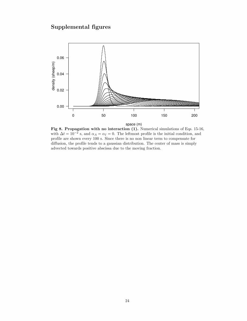
Fig 8. Propagation with no interaction (1). Numerical simulations of Eqs. 15-16,with ∆t = 10−2 s, and αA = αI = 0. The leftmost profile is the initial condition, andprofile are shown every 100 s. Since there is no non linear term to compensate fordiffusion, the profile tends to a gaussian distribution. The center of mass is simplyadvected towards positive abscissa due to the moving fraction.
24
T = 0 s
De
nsity
0 100 200 300 400
0.000
0.005
0.010
0.015
0.020
T = 450 s
De
nsity
0 100 200 300 400
0.000
0.005
0.010
0.015
0.020
T = 900 s
De
nsity
0 100 200 300 400
0.000
0.005
0.010
0.015
0.020
T = 1350 s
De
nsity
0 100 200 300 400
0.000
0.005
0.010
0.015
0.020
T = 1800 s
S (m)
De
nsity
0 100 200 300 400
0.000
0.005
0.010
0.015
0.020
T = 7200 s
S (m)
De
nsity
0 200 400 600 800 1000
0.000
0.005
0.010
0.015
0.020
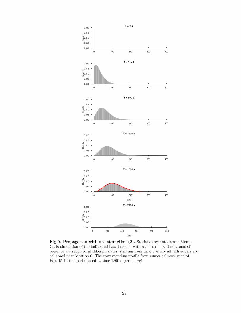
Fig 9. Propagation with no interaction (2). Statistics over stochastic MonteCarlo simulation of the individual-based model, with αA = αI = 0. Histograms ofpresence are reported at different dates, starting from time 0 where all individuals arecollapsed near location 0. The corresponding profile from numerical resolution ofEqs. 15-16 is superimposed at time 1800 s (red curve).
25
−100 −50 0 50 100
0.0
0.2
0.4
0.6
0.8
1.0
C
bs
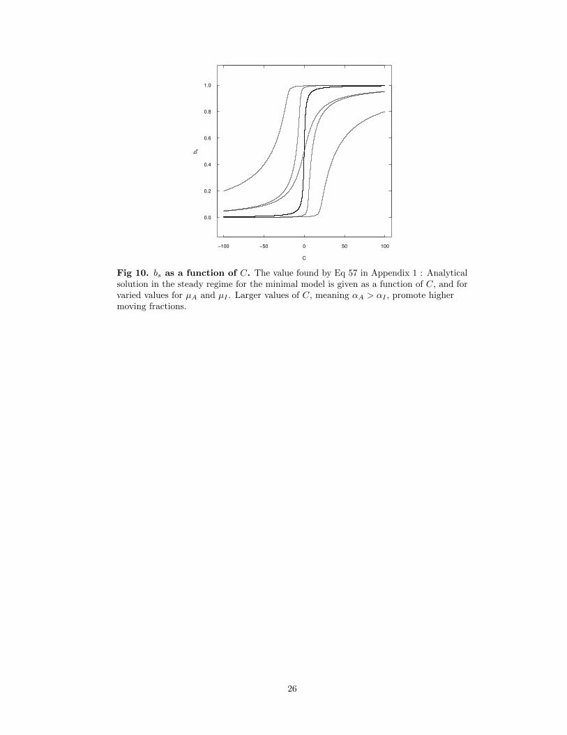
Fig 10. bs as a function of C. The value found by Eq 57 in Appendix 1 : Analyticalsolution in the steady regime for the minimal model is given as a function of C, and forvaried values for µA and µI . Larger values of C, meaning αA > αI , promote highermoving fractions.
26
Movie S1 Typical motion behaviour of a group of 3 sheep. The evolution of3 sheep is reported every second in field coordinates. Each sheep has been assigned acolour. Individuals are nearly motionless most of the time, while they are devoted tograzing. These grazing phases are separated by collective moves that translocate thegroup over several meters at high speed. A clear event of such a collective motionhappens from frame 318 to frame 344.
Movie S2 Stochastic simulations for a group of N=4 sheep with biologicalparameters given in the main text. One realisation is given in each frame. The 1Dposition of each individual is presented as a function of time. Horizontal progressionindicates a motionless individual. Oblique progression indicates a moving individual.The aggregation in time of oblique events indicates the synchronisation of motionphases.
Movie S3 Stochastic simulations for a group of N=4 sheep, like in MovieS2, but with a dominant spontaneous departure parameter. The couplingparameters have been downscaled to αA = 0.001 and αI = 0.016. As a consequence,individual are mainly driven by independent switching decisions, which results in theloss of synchronisation and group dispersion over ten of meters.
Movie S4 Illustration of the propagation of a group of N=32 sheeppredicted by the model, illustrating that groups can be seen to progress as a wholeat some fraction of the individual speed whilst each individual is either stopped ormoving at full speed. Stopped individuals are reported by black dots, and movingindividuals are reported by red dots. The panel above reports the number of individualsin motion. The dotted line indicates the average of this number over time.
Movie S5 Numerical simulations of Eqs. 15-16, with ∆t = 10−2 s, forvarious initial conditions. Four different initial conditions were tested: starting atframe 1, the group starts loosely dispersed over 20-30 m with all individuals in thestopped state, from frame 116 the group starts with the same dispersion but with allindividuals in the moving state, from frame 210 the group is split into two separatedgroups with moving individuals in the group ahead, and from frame 348 with movingindividuals in the group behind. All simulations converge to the same traveling pulse.
Movie S6 Numerical simulations of Eqs. 15-16, with ∆t = 10−2 s, withanalytical solution superimposed. The upper panel shows the numericalsimulations of the Boltzmann-like equations using the minimal model (βA = βI = 1 andγA = γI = 0, N = 4, spontaneous rates unchanged). Two sets of parameters arereported: αA = αI = 0.5 from frame 1, and αA = 0.8, αI = 0.2 from frame 202. Thelower panel shows a zoom of the numerical profile, centred on the center of mass (blackcurve) and the analytical traveling pulse (red curve). Since αA + αI remains equal to 1in both case, the analytical solution is the same for the density profile. However, thepropagating speed is affected (it is faster for the case with dominant activatingstimulation) and the route to converge towards the analytical solution is different.
Movie S7 Recovering the traveling pulse propagation after a perturbation.We use the IBM simulation program to test how the group react to a perturbation. Here,the perturbation is the extinction of interactions for a given period of time. The groupstarts unperturbed. Stopped individuals are reported in black and moving individuals inred. In the beginning, we set the camera in constant speed motion tuned to the averagespeed of the group. We can see the group ahead of sync or behind of sync in regards to
27
this moving camera frame, but still it keeps progressing on average. At time 1000 (frame1000), the interactions are set off, and the camera is stopped while its angle is enlargedto cover a larger area. From that time, individuals progress at their own pace, leadingto group dispersal (by advection/diffusion). At time 1999 (frame 1999), interactions arerestored. The groups then tends to regain its cohesion, illustrating that the ones aheadwaits for the one behind to progress before they move again. At times near 2500, thegroup has reached its steady regime density and recovers the steady regime propagation.The camera is set back in motion at time 2550 and its angle restored to its initial value.
Acknowledgments
This work was supported by French Agence Nationale de la Recherche (ANR) GrantBLAN07-3 200418.
References
Attanasi et al., 2015. Attanasi, A., Cavagna, A., Castello, L. D., Giardina, I., Jelic,A., Melillo, S., Parisi, L., Pohl, O., Shen, E., Viale, M., and Giardina, I. (2015).Emergence of collective changes in travel direction of starling flocks from individualbirds’ fluctuations. J. R. Soc. Interface, 12:1–11, 1410.3330.
Attanasi et al., 2014. Attanasi, A., Cavagna, A., Del Castello, L., Giardina, I.,Grigera, T. S., Jelic, A., Melillo, S., Parisi, L., Pohl, O., Shen, E., and Viale, M.(2014). Information transfer and behavioural inertia in starling flocks. Nat. Phys.,10(9):691–696, 1303.7097.
Ballerini et al., 2008a. Ballerini, M., Cabibbo, N., Candelier, R., Cavagna, A.,Cisbani, E., Giardina, I., Lecomte, V., Orlandi, A., Parisi, G., Procaccini, A., Viale,M., and Zdravkovic, V. (2008a). Interaction ruling animal collective behaviordepends on topological rather than metric distance: evidence from a field study.Proc. Natl. Acad. Sci. U. S. A., 105(4):1232–1237.
Ballerini et al., 2008b. Ballerini, M., Cabibbo, N., Candelier, R., Cavagna, A.,Cisbani, E., Giardina, I., Lecomte, V., Orlandi, A., Parisi, G., Procaccini, A., Viale,M., and Zdravkovic, V. (2008b). Interaction ruling animal collective behaviordepends on topological rather than metric distance: evidence from a field study.Proc. Natl. Acad. Sci. U. S. A., 105(4):1232–7.
Barberis and Peruani, 2016. Barberis, L. and Peruani, F. (2016). Large-ScalePatterns in a Minimal Cognitive Flocking Model: Incidental Leaders, NematicPatterns, and Aggregates. Phys. Rev. Lett., 117(24):1–6.
Bertin, 2017. Bertin, E. (2017). Theoretical approaches to the steady-state statisticalphysics of interacting dissipative units. J. Phys. A Math. Theor., 50(8):083001.
Bertin et al., 2009. Bertin, E., Droz, M., and Gregoire, G. (2009). Hydrodynamicequations for self-propelled particles: microscopic derivation and stability analysis.J. Phys. A Math. Theor., 42(44):445001, 0907.4688.
Bialek et al., 2014. Bialek, W., Cavagna, A., Giardina, I., Mora, T., Pohl, O.,Silvestri, E., Viale, M., and Walczak, A. M. (2014). Social interactions dominatespeed control in poising natural flocks near criticality. Proc. Natl. Acad. Sci. U. S.A., 111(20):7212–7.
28
Bialek et al., 2012. Bialek, W., Cavagna, A., Giardina, I., Mora, T., Silvestri, E.,Viale, M., and Walczak, A. M. (2012). Statistical mechanics for natural flocks ofbirds. Proc. Natl. Acad. Sci. U. S. A., 109(13):4786–91.
Calovi et al., 2015. Calovi, D. S., Lopez, U., Schuhmacher, P., Chate, H., andTheraulaz, G. (2015). Collective response to perturbations in a data-driven fishschool model. J. R. Soc. Interface, 12:20141362, arXiv:1409.6430v2.
Carrillo et al., 2014. Carrillo, J. A., Eftimie, R., and Hoffmann, F. K. O. (2014).Non-local kinetic and macroscopic models for self-organised animal aggregations.Kinet. Relat. Model., 8(3):1–29, arXiv:1407.2099v1.
Cavagna et al., 2016. Cavagna, A., Conti, D., Giardina, I., Grigera, T. S., Melillo, S.,and Viale, M. (2016). Spatio-temporal correlations in models of collective motionruled by different dynamical laws. Phys. Biol., 13(6):065001, 1605.09628.
Chate et al., 2008. Chate, H., Ginelli, F., Gregoire, G., and Raynaud, F. (2008).Collective motion of self-propelled particles interacting without cohesion. Phys. Rev.E - Stat. Nonlinear, Soft Matter Phys., 77(4):1–15, 0712.2062.
Eftimie, 2012. Eftimie, R. (2012). Hyperbolic and kinetic models for self-organizedbiological aggregations and movement: A brief review. J. Math. Biol., 65(1):35–75.
Eftimie et al., 2007a. Eftimie, R., de Vries, G., and Lewis, M. a. (2007a). Complexspatial group patterns result from different animal communication mechanisms.Proc. Natl. Acad. Sci. U. S. A., 104(17):6974–6979.
Eftimie et al., 2007b. Eftimie, R., De Vries, G., Lewis, M. A., and Lutscher, F.(2007b). Modeling group formation and activity patterns in self-organizingcollectives of individuals. Bull. Math. Biol., 69(5):1537–1565.
Gautrais et al., 2012. Gautrais, J., Ginelli, F., Fournier, R., Blanco, S., Soria, M.,Chate, H., and Theraulaz, G. (2012). Deciphering interactions in moving animalgroups. PLoS Comput. Biol., 8(9):e1002678.
Ginelli et al., 2010. Ginelli, F., Peruani, F., Bar, M., and Chate, H. (2010).Large-scale collective properties of self-propelled rods. Phys. Rev. Lett.,104(18):184502, 0911.1924.
Ginelli et al., 2015. Ginelli, F., Peruani, F., Pillot, M.-H., Chate, H., Theraulaz, G.,and Bon, R. (2015). Intermittent collective dynamics emerge from conflictingimperatives in sheep herds. Proc. Natl. Acad. Sci., 112(41):12729–12734.
Hemelrijk and Hildenbrandt, 2014. Hemelrijk, C. K. and Hildenbrandt, H. (2014).Scale-Free Correlations, Influential Neighbours and Speed Control in Flocks ofBirds. J. Stat. Phys., 158(3):563–578.
Hemelrijk and Hildenbrandt, 2015. Hemelrijk, C. K. and Hildenbrandt, H. (2015).Diffusion and topological neighbours in flocks of starlings: Relating a model toempirical data. PLoS One, 10(5).
Hemelrijk et al., 2015. Hemelrijk, C. K., van Zuidam, L., and Hildenbrandt, H.(2015). What underlies waves of agitation in starling flocks. Behav. Ecol. Sociobiol.,69(5):755–764.
Herbert-Read, 2016. Herbert-Read, J. E. (2016). Understanding how animal groupsachieve coordinated movement. J. Exp. Biol., 219(19):2971–2983.
29
Jiang et al., 2017. Jiang, L., Giuggioli, L., Perna, A., Escobedo, R., Lecheval, V.,Sire, C., Han, Z., and Theraulaz, G. (2017). Identifying influential neighbors inanimal flocking. PLOS Comput. Biol., 13(11):e1005822.
Katz et al., 2011. Katz, Y., Tunstrøm, K., Ioannou, C. C., Huepe, C., Couzin, I. D.,Tunstrom, K., Ioannou, C. C., Huepe, C., and Couzin, I. D. (2011). Inferring thestructure and dynamics of interactions in schooling fish. Proc. Natl. Acad. Sci.,108:18720–18725.
Kerner and Osipov, 1994. Kerner, B. S. and Osipov, V. V. (1994). Autosolitons,volume 61. Springer Netherlands, Dordrecht.
Kramer and McLaughlin, 2001. Kramer, D. L. and McLaughlin, R. L. (2001). TheBehavioral Ecology of Intermittent Locomotion1. Am. Zool., 41(2):137–153.
Kuwayama and Ishida, 2013. Kuwayama, H. and Ishida, S. (2013). Biological solitonin multicellular movement. Sci. Rep., 3:3–7.
Lopez et al., 2012. Lopez, U., Gautrais, J., Couzin, I. D., and Theraulaz, G. (2012).From behavioural analyses to models of collective motion in fish schools. InterfaceFocus, 2(6):693–707.
Mogilner and Edelstein-Keshet, 1999. Mogilner, A. and Edelstein-Keshet, L. (1999).A non-local model for a swarm. J. Math. Biol., 38(6):534–570.
Peshkov et al., 2014. Peshkov, A., Bertin, E., Ginelli, F., and Chate, H. (2014).Boltzmann-Ginzburg-Landau approach for continuous descriptions of genericVicsek-like models. Eur. Phys. J. Spec. Top., 223(7):1315–1344, 1404.3275.
Petit et al., 2009. Petit, O., Gautrais, J., Leca, J.-B., Theraulaz, G., andDeneubourg, J.-L. (2009). Collective decision-making in white-faced capuchinmonkeys. Proc. R. Soc. B Biol. Sci., 276(1672):3495–3503.
Pillot et al., 2011. Pillot, M.-H., Gautrais, J., Arrufat, P., Couzin, I. D., Bon, R., andDeneubourg, J.-L. (2011). Scalable rules for coherent group motion in a gregariousvertebrate. PLoS One, 6(1):e14487.
Pineda et al., 2015. Pineda, M., Weijer, C. J., and Eftimie, R. (2015). Modelling cellmovement, cell differentiation, cell sorting and proportion regulation inDictyostelium discoideum aggregations. J. Theor. Biol., 370(0):135–150.
Purwins et al., 2005. Purwins, H., Bodeker, H., and Liehr, A. (2005). DissipativeSolitons in Reaction-Diffusion Systems. In Dissipative Solitons, volume 308, pages267–308. Springer Berlin Heidelberg, Berlin, Heidelberg.
Purwins et al., 2010. Purwins, H. G., Bodeker, H. U., and Amiranashvili, S. (2010).Dissipative solitons. Advances in Physics, 59(5):485–701.
Rimer and Ariel, 2017. Rimer, O. and Ariel, G. (2017). Kinetic order-disordertransitions in a pause-and-go swarming model with memory. J. Theor. Biol.,419:90–99.
Rosenthal et al., 2015. Rosenthal, S. B., Twomey, C. R., Hartnett, A. T., Wu, H. S.,and Couzin, I. D. (2015). Revealing the hidden networks of interaction in mobileanimal groups allows prediction of complex behavioral contagion. Proc. Natl. Acad.Sci., 112(15):4690–4695.
30
Saragosti et al., 2010. Saragosti, J., Calvez, V., Bournaveas, N., Buguin, A.,Silberzan, P., and Perthame, B. (2010). Mathematical description of bacterialtraveling pulses. PLoS Comput. Biol., 6(8), 0912.1792.
Saragosti et al., 2011. Saragosti, J., Calvez, V., Bournaveas, N., Perthame, B.,Buguin, A., and Silberzan, P. (2011). Directional persistence of chemotactic bacteriain a traveling concentration wave. Proc. Natl. Acad. Sci., 108(39):16235–16240.
Sumpter, 2006. Sumpter, D. J. T. (2006). The principles of collective animalbehaviour. Philos. Trans. R. Soc. Lond. B. Biol. Sci., 361(1465):5–22.
Sumpter, 2010. Sumpter, D. J. T. (2010). Collective Animal Behavior. Princeton,NJ: Princeton University Press.
Tindall et al., 2008. Tindall, M. J., Maini, P. K., Porter, S. L., and Armitage, J. P.(2008). Overview of mathematical approaches used to model bacterial chemotaxis II:Bacterial populations. Bulletin of Mathematical Biology, 70(6):1570–1607.
Toulet et al., 2015. Toulet, S., Gautrais, J., Bon, R., and Peruani, F. (2015).Imitation Combined with a Characteristic Stimulus Duration Results in RobustCollective Decision-Making. PLoS One, 10(10):e0140188.
Tunstrøm et al., 2013. Tunstrøm, K., Katz, Y., Ioannou, C. C., Huepe, C., Lutz,M. J., and Couzin, I. D. (2013). Collective States, Multistability and TransitionalBehavior in Schooling Fish. PLoS Comput. Biol., 9(2):e1002915.
Vicsek et al., 1995. Vicsek, T., Czirok, A., Ben-Jacob, E., Cohen, I., and Shochet, O.(1995). Novel type of phase transition in a system of self-driven particles. Phys. Rev.Lett., 75(6):4–7.
Vicsek and Zafeiris, 2012. Vicsek, T. and Zafeiris, A. (2012). Collective motion.Phys. Rep., 517(3-4):71–140.
31