SHED: Shape Edit Distance for Fine-grained Shape Similarity

Yanir Kleiman1 Oliver van Kaick1,2 Olga Sorkine-Hornung3 Daniel Cohen-Or11Tel Aviv University 2Carleton University 3ETH Zurich

Abstract

Computing similarities or distances between 3D shapes is a crucialbuilding block for numerous tasks, including shape retrieval, ex-ploration and classification. Current state-of-the-art distance mea-sures mostly consider the overall appearance of the shapes and areless sensitive to fine changes in shape structure or geometry. Wepresent shape edit distance (SHED) that measures the amount ofeffort needed to transform one shape into the other, in terms of re-arranging the parts of one shape to match the parts of the othershape, as well as possibly adding and removing parts. The shapeedit distance takes into account both the similarity of the overallshape structure and the similarity of individual parts of the shapes.We show that SHED is favorable to state-of-the-art distance mea-sures in a variety of applications and datasets, and is especially suc-cessful in scenarios where detecting fine details of the shapes isimportant, such as shape retrieval and exploration.

CR Categories: I.3.5 [Computer Graphics]: Computational Ge-ometry and Object Modeling—Geometric algorithms, languages,and systems.

Keywords: Shape similarity, intra-class retrieval, edit distance.

1 Introduction

With the growth of on-line shape repositories in recent years, thereis an increasing need to organize and efficiently explore large col-lections of 3D shapes [Ovsjanikov et al. 2011; Huang et al. 2013b;Kim et al. 2013; Kleiman et al. 2013; Averkiou et al. 2014]. Thequestion underlying this task, and a fundamental question in shapeanalysis, is how to compare shapes and measure their similarity. Infact, the choice of an appropriate similarity measure is in the coreof many algorithms that handle 3D shapes. In this regard, previ-ous work has focused on the development of similarity measuresfor classification of shapes into broad sets of categories [Tangelderand Veltkamp 2008], but little attention has been given to estimat-ing the similarity between shapes that belong to the same class.That is, detection of inter-class differences has been emphasizedover quantification of intra-class differences. With the large repos-itories available today, organization and exploration of families ofshapes has become as important as categorizing shapes into dif-ferent classes, and such tasks require an estimation of fine-grainedshape similarities.

In this work, we introduce shape edit distance to measure similar-ities between shapes. Intuitively, the shape edit distance (SHED)

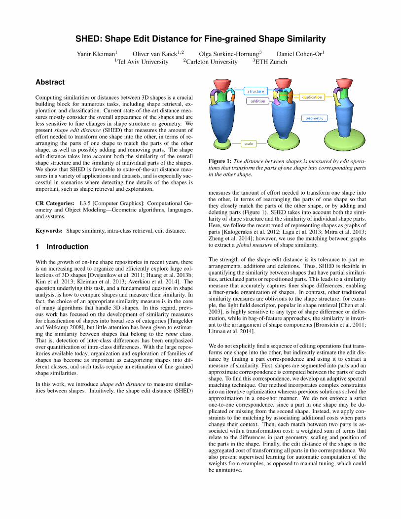
Figure 1: The distance between shapes is measured by edit opera-tions that transform the parts of one shape into corresponding partsin the other shape.

measures the amount of effort needed to transform one shape intothe other, in terms of rearranging the parts of one shape so thatthey closely match the parts of the other shape, or by adding anddeleting parts (Figure 1). SHED takes into account both the simi-larity of shape structure and the similarity of individual shape parts.Here, we follow the recent trend of representing shapes as graphs ofparts [Kalogerakis et al. 2012; Laga et al. 2013; Mitra et al. 2013;Zheng et al. 2014]; however, we use the matching between graphsto extract a global measure of shape similarity.

The strength of the shape edit distance is its tolerance to part re-arrangements, additions and deletions. Thus, SHED is flexible inquantifying the similarity between shapes that have partial similari-ties, articulated parts or repositioned parts. This leads to a similaritymeasure that accurately captures finer shape differences, enablinga finer-grade organization of shapes. In contrast, other traditionalsimilarity measures are oblivious to the shape structure: for exam-ple, the light field descriptor, popular in shape retrieval [Chen et al.2003], is highly sensitive to any type of shape difference or defor-mation, while in bag-of-feature approaches, the similarity is invari-ant to the arrangement of shape components [Bronstein et al. 2011;Litman et al. 2014].

We do not explicitly find a sequence of editing operations that trans-forms one shape into the other, but indirectly estimate the edit dis-tance by finding a part correspondence and using it to extract ameasure of similarity. First, shapes are segmented into parts and anapproximate correspondence is computed between the parts of eachshape. To find this correspondence, we develop an adaptive spectralmatching technique. Our method incorporates complex constraintsinto an iterative optimization whereas previous solutions solved theapproximation in a one-shot manner. We do not enforce a strictone-to-one correspondence, since a part in one shape may be du-plicated or missing from the second shape. Instead, we apply con-straints to the matching by associating additional costs when partschange their context. Then, each match between two parts is as-sociated with a transformation cost: a weighted sum of terms thatrelate to the differences in part geometry, scaling and position ofthe parts in the shape. Finally, the edit distance of the shape is theaggregated cost of transforming all parts in the correspondence. Wealso present supervised learning for automatic computation of theweights from examples, as opposed to manual tuning, which couldbe unintuitive.

We demonstrate the advantage of using SHED with a series of ex-periments. First, we evaluate SHED in a quantitative manner byconstructing categorization trees that can be used for shape explo-ration. We compare these trees to the trees generated using otherstate-of-the-art similarity measures, as well as ground truth treescreated by expert users. In addition, we cluster shapes into a pre-defined number of clusters and compare the results to clusters gen-erated from the ground truth trees. These evaluations demonstratethat the similarity estimated by SHED is preferable to other dis-tance measures and leads to a more intuitive shape organization inthe intra-class context. In the inter-class context, we perform shaperetrieval according to SHED and show that it yields comparableresults to state-of-the-art similarity measures. Finally, in settingswhere ground truth data is not well defined, we show qualitative re-sults of nearest neighbors queries and embeddings of sets of shapes.

2 Related work

Our work comprises ideas such as shape comparison, graph editdistances and part-based matching, which we discuss as follows.

Shape comparison, retrieval and exploration. There has beenmuch work on the development of shape similarity measures thatcan be used for retrieval, exploration, or any type of shape com-parison [Tangelder and Veltkamp 2008]. In terms of shape retrievaland categorization, state-of-the-art approaches that currently givethe best performance are a combination of the light field descrip-tor with bag-of-features and metric learning approaches [Li et al.2012]. For intra-class organization, Xu et al. [2010] cluster a setof shapes into different groups by factoring out the effect of non-homogeneous part scaling and then establishing a correspondencebetween shape parts. Huang et al. [2013a] present an approach forfine-grained labeling of shape collections. Similarly to our work,their goal is to learn a distance metric within a class of shapes tocapture finer shape differences. However, their method follows adifferent paradigm than our work: the shapes are globally alignedwith an affine transformation followed by local deformations, andthe metric is learned on the aligned shapes. Individual parts ob-tained from segmentation and their transformation are not consid-ered as in our approach. In the more restricted context of isometricmatching, there has been much activity in deriving signatures forshape comparison, such as GPS embedding [Rustamov 2007] orheat kernel signature [Ovsjanikov et al. 2010]. Kurtek et al. [2013]define a shape space and metric that capture more comprehensivedeformations than nearly isometric, but require surfaces of the sametopology. Bag-of-feature approaches [Bronstein et al. 2011; Litmanet al. 2014] are considered state of the art for retrieval of non-rigidisometric shapes. The goal of these methods is to retrieve shapeswith similar topology from a collection of shapes in the same class,such as human models in different poses. Hence, these methods arenot suitable for comparison of shapes with different part composi-tion, structure or topology, which is the focus of our work.

Shape exploration necessitates not only the estimation of the sim-ilarity of shapes to a query shape, but also a way of organizingthe shapes. Thus, different strategies have been proposed for ex-ploration, such as the use of a deformable template [Ovsjanikovet al. 2011], region selection [Kim et al. 2012], dynamically adaptedviews of close neighborhoods [Kleiman et al. 2013], or parameter-ization of the template space [Averkiou et al. 2014]. In the work ofHuang et al. [2013b], the goal is to obtain a qualitative organizationof a collection of shapes, since an organization based on a singlesimilarity measure is not always meaningful when comparing bothsimilar and dissimilar shapes. Likewise, our goal is to properlycapture both inter- and intra-class differences. However, instead ofaggregating the scores of several similarity measures, we developan edit distance to estimate the shape similarity.

Graphs of parts for shape analysis. The idea of describing 2Dshapes and images as graphs of parts has appeared prominently inthe field of computer vision. A few representative works includematching shapes according to shock graphs [Sebastian et al. 2004]and skeletons [Sundar et al. 2003], and matching images accordingto graphs that represent their segmentations [Harchaoui and Bach2007]. In the graphics literature, comparing shapes by matchinggraphs was utilized for consistent joint segmentation [Huang et al.2011] and co-segmentation [Sidi et al. 2011] of a set of shapes.A group of works has estimated the similarity between shapes bymatching Reeb graphs, which are constructed from functions de-fined on manifold shapes [Hilaga et al. 2001; Barra and Biasotti2013]. Other works have explicitly segmented shapes and createdgraphs of segments, with applications in shape synthesis [Kaloger-akis et al. 2012] and semantic correspondence [Laga et al. 2013].These works are directly related to the idea of modeling shapes bycombining parts from different models [Funkhouser et al. 2004].Templates or part arrangements have also been learned from col-lections, although these do not explicitly represent the connectivitybetween parts [Kim et al. 2013; Zheng et al. 2014]. The fundamen-tal difference of our approach to these representative works is thatwe use the matching between two graphs of parts as input to esti-mate the overall similarity between two shapes; the correspondencebetween the graphs is the base for a distance measure that enablesus to quantify finer shape differences.

Graph matching and integer programming. The graph match-ing problem is commonly posed as an integer quadratic program-ming problem, which is NP-hard. There is a large body of workregarding the relaxation of such problems to a tractable convexquadratic programming optimization. Two prominent works in thisarea are the spectral correspondence presented by Leordeanu andHebert [2005] and a relaxation of the quadratic optimization byusing bounding linear integer optimizations, proposed by Berg etal. [2005]. These relaxations often yield good results in practicein the one-to-one matching scenario. However, performing gra-dient descent from a continuous relaxation of the integer prob-lem has been shown to yield non-optimal permutations in mostcases [Lyzinski et al. 2015]. Indeed, the above methods performpoorly in our one-to-many scenario where a part can correspondto several parts in the other shape. Recently, Kezurer et al. [2015]suggested lifting the problem to a higher dimension, followed bya linear semi-definite relaxation. However, their method is com-putationally expensive and does not extend easily to one-to-manyscenarios. Bommes et al. [2012] perform iterative relaxation of theproblem where in each iteration a single integer constraint is addedto the optimization. We follow a similar approach, but instead ofadding hard constraints in each step, we adjust the objective func-tion to give precedence to solutions which are compatible with pre-viously selected matches.

Graph edit distance. The graph edit distance has been used tofind a correspondence between graphs in several areas of visualcomputing, such as computer vision and medical imaging [Gaoet al. 2010]. The idea of an edit distance is attractive because itposes the problem of matching two graphs as finding a sequenceof operations that transforms one graph into the other. The editdistance can consider not only the matching of similar nodes andedges, but also their addition, duplication and deletion. However,finding the minimal edit distance is NP-hard, so different heuris-tics have been proposed to compute it. A common technique isto use a graph kernel that estimates the similarity between twonodes according to their attributes and their neighborhoods in thegraphs [Neuhaus and Bunke 2007]. Our shape edit distance doesnot require an explicit sequence of operations, but an aggregationof all the changes necessary to transform one shape into the other.

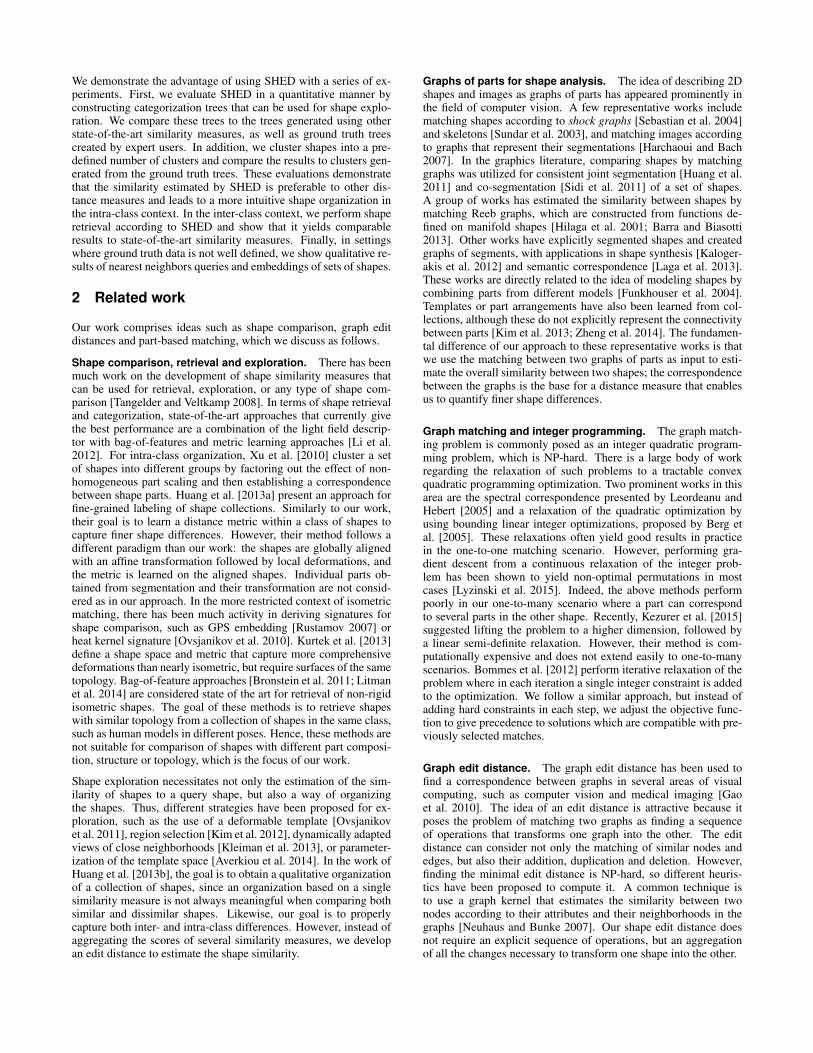
Figure 2: Difference between the semantic segmentation of twoshapes in (a) and (b), and their nearly convex decomposition in (c)and (d). Note how, in (a) and (b), the bounding boxes of the partscorresponding to the candle supports have considerably differentsizes. In (c) and (d), both supports are composed of small nearlyconvex segments with similar sizes.

In the context of computer graphics, Fisher et al. [2011] usedgraph kernels to estimate the similarity between graphs represent-ing scenes composed of multiple objects. In addition, Denning andPellacini [2013] proposed a technique based on the edit distance toquantify localized differences between two models. Their methodis better suited for comparing models generated by editing the samesource shape. On the other hand, our work is aimed at computingthe similarity between any pair of shapes. We derive the edit dis-tance directly from a correspondence between graph nodes, as op-posed to the methods above based on graph kernels. In addition,we do not require a one-to-one correspondence between the shapeparts, but find a one-to-many correspondence and quantify the editdistance without explicitly searching for a sequence of editing op-erations. We explain the details in the next section.

3 Shape edit distance

Input, output, and shape representation. The edit distancemeasure takes as input two shapes and returns a real number rep-resenting the distance (dissimilarity) between the shapes. The dis-tance is lower for shapes that have similar part geometry and struc-ture, taking into account part rearrangements and partial correspon-dence, and higher for shapes that differ in these aspects.

We represent each shape as a collection of parts and connectionsamong these parts, i.e., a graph of parts. Our method is generic andcan take as input different shape representations, although in thiswork we represent the shapes as triangle meshes. The first step inour method is the partitioning of input meshes into parts. One pos-sibility is to use semantic segmentation techniques [Shapira et al.2008; Shamir 2008]. However, semantic parts do not have a cleardefinition and can greatly vary among different shapes. Moreover,a semantic part can have a complex geometry, making its compar-ison to other semantic parts non-trivial (Figure 2). In a sense, theproblem of comparing two complex segments can be as involved asthat of comparing two shapes. Instead, we segment the shapes intosimpler primitives that can be more easily analyzed. For this task,we use the recent weakly-convex decomposition technique of vanKaick et al. [2014], which partitions the input shapes into nearlyconvex parts. Nearly convex parts are easier to analyze, since theyhave a simpler geometry and can be approximated well by theirbounding boxes (Figure 2). In addition, the convex decompositionof a shape is robust to small changes in the shape.

Our method also supports using a manual segmentation of theshapes into parts, if such data is available. However, the resultsin this paper were produced using the automatic weakly-convex de-composition to provide a complete solution. The part graph is de-fined by creating a node for each nearly convex part of the shape,and an edge between adjacent parts in the shape segmentation.

Part similarities and matching. Given two shapes representedas graphs of parts, our goal is to find a set of editing operations thattransform the parts of one shape into the parts of the other. Pos-sible editing operations include deforming, displacing, duplicating,adding, or removing parts. Then, a cost is associated with eachediting operation based on the extent of the transformation. Theediting costs are aggregated to produce the final shape edit distancebetween the two input shapes.

In SHED, we derive the set of editing operations from a mappingbetween the parts, since we can associate each pairwise match witha single operation. This mapping depends on the similarity of partsto each other as well as their context and the structure of the shape.For example, two parts with different geometry can be matched iftheir neighborhood is similar. On the other hand, two parts in differ-ent locations in the shape can be matched if their geometry is sim-ilar. Thus, the mapping of each part depends not only on the partproperties, but on the mapping of all other parts of the shape. Thismakes the problem of finding the correct matching intractable, soan approximate solution is necessary. To this end, we formulate ourobjective in a quadratic form by constructing unary terms for eachmatch between two parts, and binary terms for pairs of matches,representing only pairwise dependencies between matches. Then,we develop a novel adaptive spectral matching technique to find anapproximate solution for this formulation. Our technique uses sim-ilar principles as the method of Leordeanu and Hebert [2005], butinstead of solving the optimization once and applying constraints ina greedy manner, we iteratively improve the optimization by incor-porating the constraints that arise in previous steps. We explain thecomputation of the matching in detail in Section 4.

Given the mapping between two shapes, a cost can be computed foreach edit operation. The costs reflect the following aspects of shapesimilarity:

• Similarity of the geometry of the parts. For example, mor-phing a cylindrical part into another cylindrical part is lesscostly than morphing a cube into a cylinder, as the formerpair is geometrically more similar than the latter.

• Similarity of the structure of the part graphs. We allownodes to move in the part graph, with a cost proportional tothe magnitude of the structural change. Duplicated parts andadditional parts also incur additional costs as the structure ofthe shape changes.

• Scaling of the parts. The scale of each part plays a criticalrole in the global similarity of a shape; different shapes canhave similar graphs of parts where each part is scaled differ-ently relative to its neighborhood. Thus, we introduce scale-specific terms in our formulation.

To produce a scalar similarity measure between two shapes, theterms described above need to be weighted and aggregated. A ques-tion arises of how to determine the weights for each term. Shapesimilarity is a subjective measure, so different users might have dif-ferent views on which shapes are more similar, which implies thatdifferent weights are necessary. Moreover, while a set of manuallyselected weights can provide a reasonable similarity measure forall shapes, it is clearly beneficial to fine-tune the weights to bet-ter reflect the variation in a specific set. Therefore, we employ aweight learning scheme that finds the optimal weights to match aset of given distances. We elaborate on the details of the distanceformulation and the weight learning scheme in Section 5.

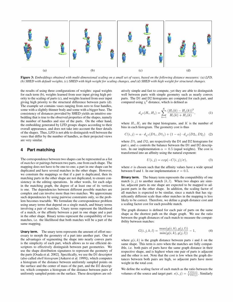
In Figure 3, we show the effect of considering these different fac-tors in the edit distance. We compare a 2D embedding created withmulti-dimensional scaling, according to the similarities given bySHED and the light field descriptor (LFD). For SHED, we show

(a) (b) (c) (d)

Figure 3: Embeddings obtained with multi-dimensional scaling on a small set of vases, based on the following distance measures: (a) LFD,(b) SHED with default weights, (c) SHED with high weight for scaling changes, and (d) SHED with high weight for structural changes.

the results of using three configurations of weights: equal weightsfor each term (b), weights learned from user input giving high pri-ority to the scaling of parts (c), and weights learned from user inputgiving high priority to the structural difference between parts (d).The example set contains vases ranging from zero to four handles,some with a slightly thinner body and some with a bigger base. Theconsistency of distances provided by SHED yields an intuitive em-bedding that is true to the observed properties of the shapes, namelythe number of handles and size of the parts. On the other hand,the embedding generated by LFD groups shapes according to theiroverall appearance, and does not take into account the finer detailsof the shapes. Thus, LFD is not able to distinguish well between thevases that differ by the number of handles, as their projected viewsare very similar.

4 Part matching

The correspondence between two shapes can be represented as a listof matches or pairings between two parts, one from each shape. Themapping does not have to be one-to-one; a part in one shape can beduplicated and have several matches in the other shape. However,we constrain the mappings so that if a part is duplicated, then itsmatching parts in the other shape are not duplicated, to ensure con-sistency in the editing operations. In other words, for each edgein the matching graph, the degree of at least one of its verticesis one. The dependencies between different possible matches arecomplex and can involve more than two matches. We approximatesuch dependencies by using pairwise constraints only, so the prob-lem becomes tractable. We formulate the correspondence problemusing unary terms that depend on a single match, and binary termsinvolving a pair of matches. Unary terms represent the likelihoodof a match, or the affinity between a part in one shape and a partin the other shape. Binary terms represent the compatibility of twomatches, i.e. the likelihood that both matches will be a part of thesame mapping.

Unary term. The unary term represents the amount of effort nec-essary to morph the geometry of a part into another part. One ofthe advantages of segmenting the shape into nearly convex partsis the simplicity of each part, which allows us to use efficient de-scriptors to effectively distinguish between part geometries. Weuse the shape distribution signatures to represent the geometry ofthe parts [Osada et al. 2002]. Specifically, we use the D1 descriptor(also called shell histogram [Ankerst et al. 1999]), which computesa histogram of the distance between uniformly sampled points onthe surface and the center of mass of the part, and the D2 descrip-tor, which computes a histogram of the distance between pairs ofuniformly sampled points on the surface. These descriptors are rel-

atively simple and fast to compute, yet they are able to distinguishwell between parts with simple geometry such as nearly convexparts. The D1 and D2 histograms are computed for each part, andcompared using χ2 distance, which is defined as

dχ2(Hi, Hj) =

K∑k=1

(Hi(k)−Hj(k))2

Hi(k) +Hj(k), (1)

where Hi, Hj are the input histograms, and K is the number ofbins in each histogram. The geometry cost is thus

C(i, j) = α · dχ2(D1i, D1j) + (1− α) · dχ2(D2i, D2j) (2)

where D1i and D2i are respectively the D1 and D2 histograms forpart i, and α controls the balance between the D1 and D2 descrip-tors. In our implementation α = 0.5 (equal weights). The cost istransformed into an affinity using the natural exponent:

U(i, j) = exp(−C(i, j)/σ), (3)

where σ is chosen such that the affinity values have a wide spreadbetween 0 and 1. In our implementation σ = 0.5.

Binary term. The binary term represents the compatibility of onematch (i, j) to another match (k, l). When two shapes are simi-lar, adjacent parts in one shape are expected to be mapped to ad-jacent parts in the other shape. In addition, the scaling factor ofall matches is expected to be similar, since a match that has sig-nificantly different scale than other matches in the mapping is lesslikely to be correct. Therefore, we define a graph distance cost anda scaling factor cost for each possible match.

The graph distance is defined for each pair of parts on the sameshape as the shortest path on the shape graph. We use the ratiobetween the graph distances of each match to measure the compat-ibility between matches:

G(i, j, k, l) =max(g(i, k), g(j, l))

min(g(i, k), g(j, l))− 1, (4)

where g(i, k) is the graph distance between parts i and k on thesame shape. This term is zero when the matches are fully compat-ible, i.e. both pairs of parts have the same graph distance in theirrespective shape, and is highest when one pair of parts is adjacentand the other is not. Note that the cost is low when the graph dis-tances between both pairs are high, so adjacent parts have moreweight in the total cost.

We define the scaling factor of each match as the ratio between thevolumes of the source and target part: s(i, j) = V OL(i)

V OL(j). Similarly

to the graph distance cost, we use the ratio between the scalingfactors of two matches as the scaling factor cost:

S(i, j, k, l) =max(s(i, j), s(k, l))

min(s(i, j), s(k, l))− 1. (5)

The binary term is defined as the affinity between two matches,which is computed from the above costs as follows:

B(i, j, k, l) = β · exp(−(G(i, j, k, l) + S(i, j, k, l))/2). (6)

The parameter β controls the weight of the binary term comparedto the unary term. If β is large, the structure of the shape takesprecedence over the geometry of parts, and if β is small, the ge-ometry of the parts is more important than the shape structure. Ifβ = 0, the only consideration is the part geometry and the corre-spondence resembles a bag-of-features approach. In our implemen-tation, β = 0.3.

Matching technique. There are several matching techniquesin the literature that find an approximate solution to pairwise-constrained correspondence problems, such as the spectral match-ing technique of Leordeanu and Hebert [2005], or the integerquadratic programming relaxation proposed by Berg et al. [2005].The main idea of these methods is that the pairwise constraints canbe presented in a quadratic form by constructing a matrix M ofn · m rows and n · m columns, where n and m are the numbersof parts in the first and second shape, respectively. The diagonalof M contains the values of the unary term U(i, j), and the val-ues outside of the diagonal of M are the binary terms B(i, j, k, l).The best correspondence is then represented by the binary vector xthat maximizes the product xTMx and does not break additionalconstraints, such as the requirement for one-to-one mapping, etc.This poses an integer quadratic programming problem, which isNP-hard, therefore different approximation methods are suggestedin the above methods.

Leordeanu and Hebert [2005] propose to first solve an un-constrained assignment problem in the continuous setting, wherex is allowed to have values in the range [0, 1]. This can be solvedeasily by setting x to the normalized principal eigenvector of M .Then, the result vector x is binarized in a greedy manner, takinginto consideration additional constraints in the process. In eachstep, the match with the highest value in x is marked, and the valuesof the match and all conflicting matches in x are reduced to zero.This process continues until all values in x are zeros, and the finalmapping is returned as the collection of marked matches. Since theconstraints are not incorporated into the cost matrix, the greedy bi-narization process is less successful when several conflicting map-pings are possible. While strictly conflicting matches are filteredout, matches which are compatible with those conflicting matchesmight still be selected since their score is computed before the con-flicting matches are discarded. This effect is most prominent in lessconstrained scenarios such as ours. For example, we allow duplica-tions of parts, but a matching in which almost all parts are matchedto the same part is valid but not desirable in most cases.

To address these issues, we introduce adaptive spectral matching,which incorporates the desired constraints directly into the objec-tive function, leading to a more consistent global solution to thecorrespondence problem. We iteratively adjust the affinity matrixM according to the constraints and re-run the eigenvector decom-position. In this way, not only conflicting matches are excludedfrom the solution, but matches that are compatible with conflictingmatches are also less likely to be selected in subsequent steps. Theiterative method starts by setting x to the principal eigenvector ofM , and then performs the following steps:

• Mark the match with the highest value in x.

• Set the affinity of the match in M to 1.

• Incorporate constraints into M , by setting the affinities ofeach conflicting match or pair of matches to zero. In our case,once a match (i, j) is selected, the compatibility of matchesthat contain part i to matches that contain part j becomes zero(i.e. the binary scores B(i, j′, i′, j) = 0 for each i′ and j′),since having both of these matches would mean that there is amany-to-many relation between parts i and j.

• Set x to the principal eigenvector of the adjusted M , and ig-nore all matches that are conflicting or were already selected.

• Repeat until there are no more valid matches.

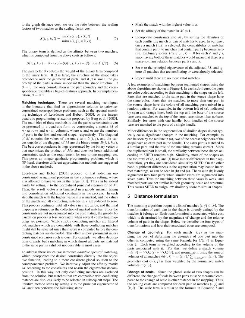
A few examples of matchings between segmented shapes using theabove algorithm are shown in Figure 4. In each sub-figure, the partsare color coded according to their matching to the shape on the left.Parts that are matched to the same part in the source shape havethe same color. Parts that are matched to more than one part inthe source shape have the colors of all matching parts mixed in arandom pattern. For example, in the bottom left of (a), indicatedby cyan and orange lines, both the top and the base of the sourcevase were matched to the top of the target vase, since it has no base.Similarly, for vases with one handle, both handles of the sourcevase are matched to the parts of a single handle.

Minor differences in the segmentation of similar shapes do not typ-ically cause significant changes in the matching. For example, ascan be seen by the red line in (a), two of the nearest neighbors of theshape have an extra part in the handle. The extra part is matched toa similar part, and the rest of the matching remains correct. Sincethe duplicated part is small, the similarity between these shapes ac-cording to SHED remains high. Similarly, most of the shapes onthe top rows of (c), (d) and (f) have minor differences in their seg-mentation, yet they are considered similar by SHED. On the otherhand, significant differences in the segmentation may lead to incor-rect matchings, as can be seen in (b) and (e). The vase in (b) is onlysegmented into four parts while similar vases are segmented intoseven parts. Thus the matching between these vases is weak, andmatched parts are not similar in their geometry, scale and structure.This causes SHED to assign low similarity score to similar shapes.

5 Distance formulation

The matching algorithm output is a list of matches (i, j) ∈M. Thetransformation of each part in the shape is directly defined by thematches it belongs to. Each transformation is associated with a costwhich is determined by the magnitude of change and the relativevolume of parts in the shape. Below we describe the four types oftransformations and how their associated costs are computed.

Change of geometry. For each match (i, j) in the map-ping, the cost of deforming the geometry of one part into theother is computed using the same formula for C(i, j) in Equa-tion 2. Each term is weighted according to the volume of theparts associated with it. For this, we define a match volumem(i, j) = V OL(i) + V OL(j), and normalize it using the sum ofvolumes of all matches m(i, j) = m(i, j)/

∑(i,j)∈Mm(i, j). The

geometry cost C(i, j) is then weighted by the normalized matchvolumes m(i, j).

Change of scale. Since the global scale of two shapes can bedifferent, the change of scale between parts must be measured com-pared to the change of scale in other matches in the mapping. Thus,the scaling costs are computed for each pair of matches (i, j) and(k, l). The scale term is similar to the formula in Equation 5 and

(a) (b) (c)

(d) (e) (f)

Figure 4: Matching between shapes. In each set, the source shape (left) is matched with three nearest neighbors according to SHED (top),and three additional shapes which are not neighbors (bottom). Multiple target parts that match the same part in the source shape are markedwith the same color (see red line, top insets in (a)). A single target part that is matched with multiple parts in the source shape is marked withmixed colors (see orange and cyan lines, bottom insets in (a)). Note that minor differences in the segmentation do not affect the matching ornearest neighbors computation (a, d, f). On the other hand, significant differences in the segmentation may lead to incorrect matching (b, e).

measures the difference between the change of scale in the twomatches:

Cs(i, j, k, l) =max(s(i, j), s(k, l))

min(s(i, j), s(k, l))− 1. (7)

Note that Cs = 0 when the scale change of the two matches isexactly the same, and Cs = 1 when the magnitude of change inone match is exactly twice than the other match. The scale costsare weighted by m(i, j) · m(k, l), such that the total weights of allthe pairs which contain match (i, j) is m(i, j).

Change of position. To detect a part that changed position, itmust be compared with its environment, so the position costs arealso computed for each pair of matches (i, j) and (k, l). We com-pare the graph distance of parts i and k in the first shape g(i, k) andthe graph distance of parts j and l in the second shape g(j, l):

Cp(i, j, k, l) = abs(g(i, k)− g(j, l)). (8)

Note that if a part is duplicated, we compare the adjacency withthe most similar instance, such that if several parts are duplicatedtogether as a group they will only be compared to parts in the samegroup. The position costs are also weighted by m(i, j) · m(k, l).

Duplication costs. When a part is duplicated, there are two ormore matches with the same part. Each of the matches incurs theabove costs if applicable. In addition, we aggregate the volume ofthe shape that is being duplicated, by summing the volume of allparts in all matches and subtracting the total volume of the shapes.The remainder is the volume of all parts (in both shapes) that appeartwice or more in the matches. The duplication cost is normalizedby the total volume of the matches, so it represents the percent ofmatches that have duplicated parts. It is formulated as:

Cd =

∑(i,j)∈M

m(i, j)−∑i∈S

V OL(i)−∑j∈T

V OL(j)∑(i,j)∈M

m(i, j), (9)

where S and T are the shapes being compared. Note that we do notdefine a cost for parts that were added, since adding a new part canbe thought of as duplicating the most similar part and morphing itto the desired shape.

Aggregation and weight learning. The shape edit distance isformulated as a weighted sum of the above costs:

SHED(S, T ) = wg ·∑

(i,j)∈Mm(i, j) · C(i, j)

+ws ·∑

(i,j)∈M,(k,l)∈Mm(i, j) · m(k, l) · Cs(i, j, k, l)

+wp ·∑

(i,j)∈M,(k,l)∈Mm(i, j) · m(k, l) · Cp(i, j, k, l)

+wd · Cd,

(10)

where wg, ws, wp and wd are the respective weights of the geom-etry term, scale term, position term and duplication term. Sincesemantic similarity between shapes is a subjective matter, it makessense to learn the values of these weights from user input. However,similarity or semantic distance between two shapes cannot be quan-tified numerically by the user. Instead, we ask users to indirectlyprovide the semantic similarity of a set of shapes by generating cat-egorization trees, which group together similar shapes in severallevels of hierarchy. For more details see Section 6. To learn theweights from the categorization trees, we extract trios of shapes,where in each trio two shapes are similar (i.e. they belong to thesame subtree of depth two), and the third shape is semantically far(i.e. it belongs to a different subtree). Each trio of shapes definesa relative relation of the form “shape A is closer to shape B thanto shape C”. Each categorization tree provides many thousands oftrios, from which we randomly select 1000 trios as a training set. Tolearn the weights from such relations, we employ a weight learningscheme suggested by Schultz and Joachims [2004]. Each relationbetween shapes A, B, and C, is transformed into a constraint of theform: D(A,C) − D(A,B) ≥ 1 where D(A,B) is the weighted

SHED LFD SPH

Figure 5: Categorization trees automatically generated for a set of vases according to SHED, LFD and SPH. The vases are colored accordingto their shape style. Note that the organization of shapes is more consistent when using SHED (3 categorization errors) than when using LFDor SPH (6 categorization errors each), as seen by the number of shapes with a different color than their lowest level neighbors in the tree.

Figure 6: Comparison of automatically generated trees to ground truth trees, according to the average difference in the degree of separation.

distance between shapes A and B. Then, a convex quadratic op-timization is formulated and solved similarly to a support vectormachine. For more details see [Schultz and Joachims 2004].

Using this method, we can fine tune the weights for a specific set ofshapes such as lamps or vases. For example, the scaling differencesbetween parts affects the semantic distance between lamps morethan it affects the semantic distance between vases. Alternatively,we can use trios from categorization trees of several sets of shapesto learn a global set of weights. Using this method, we propose aset of default weights (see Table 1) that would approximate well thesemantic similarity of any set of shapes. Note that these weightsalso reflect the relations between the different units in which thedifferent costs are measured.

6 Evaluation

The distance between two shapes cannot be directly measured orestimated numerically by a human observer, hence evaluating theaccuracy of a similarity measure is somewhat challenging. Still,we are able to compare SHED with state-of-the-art distance mea-sures, namely the light field descriptor (LFD) [Chen et al. 2003]and the spherical harmonic descriptor (SPH) [Kazhdan et al. 2003],and demonstrate its success in various applications. We evaluate theresults quantitatively using ground truth data for shape explorationand clustering, and qualitatively for nearest neighbors queries andembedding, where ground truth data is not well defined.

Datasets. We evaluate SHED using three sets of shapes from theCOSEG dataset [Wang et al. 2012] and three sets from the PrincetonSegmentation Benchmark (PSB) [Chen et al. 2009]. In addition,we collected a set of airplanes from Google Warehouse and other

online resources. The set of airplanes and the sets in the COSEGdataset were enriched by introducing finer intra-class variation. Theenriched sets include 100 lamps, 80 vases, 70 airplanes, and 40candelabra, and contain shapes that vary in their part composition,geometry, and articulation. The PSB sets include 20 humans, 20hands and 20 Teddy bears, which vary mostly in articulation.

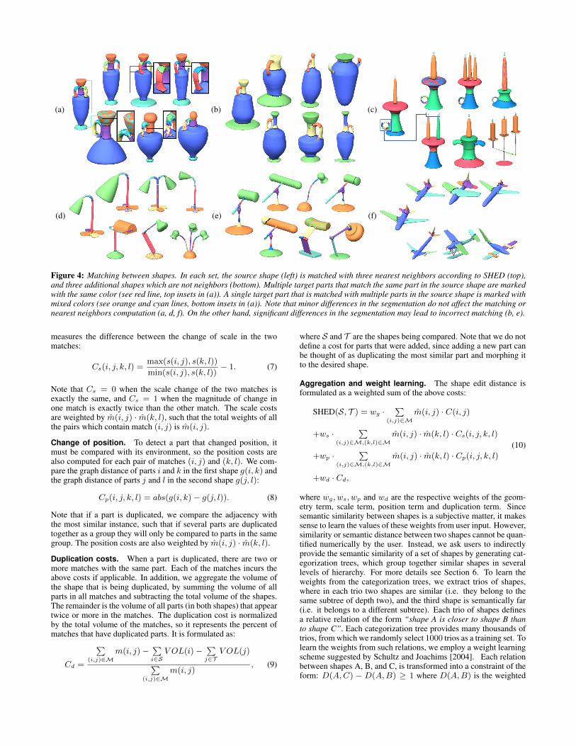
Categorization trees. We present an application where catego-rization trees of shapes are automatically generated for each en-riched set. The resulting trees hierarchically organize the shapes ina set and can be used for exploration. The trees are created usingSelf-Tuning Spectral Clustering [Zelnik-Manor and Perona 2004],which is a non-parametric clustering method, i.e., the number ofclusters in each set is selected automatically. We used this methodrecursively to build a categorization tree for each distance measure(SHED, LFD, and SPH). An example of the generated trees on asubset of shapes is presented in Figure 5, where the shapes are col-ored according to their shape style. Note that the tree generatedusing SHED has fewer categorization errors. The generated treesfor the full sets can be found in the supplementary material.

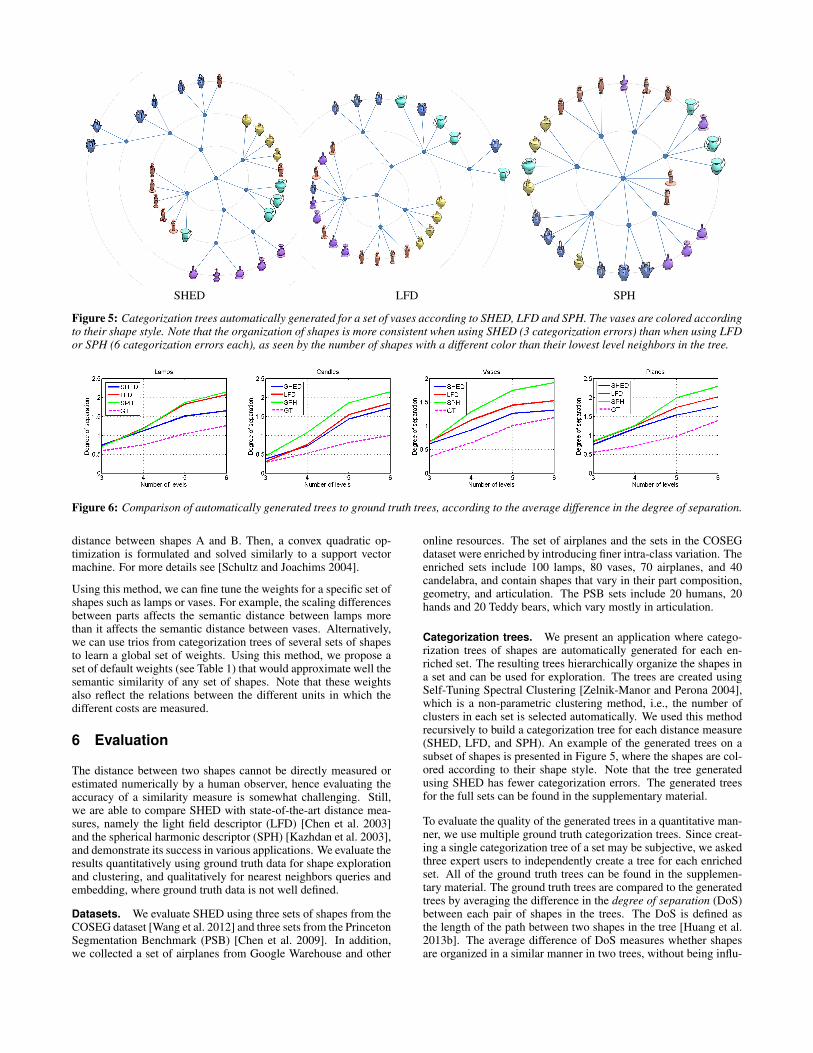
To evaluate the quality of the generated trees in a quantitative man-ner, we use multiple ground truth categorization trees. Since creat-ing a single categorization tree of a set may be subjective, we askedthree expert users to independently create a tree for each enrichedset. All of the ground truth trees can be found in the supplemen-tary material. The ground truth trees are compared to the generatedtrees by averaging the difference in the degree of separation (DoS)between each pair of shapes in the trees. The DoS is defined asthe length of the path between two shapes in the tree [Huang et al.2013b]. The average difference of DoS measures whether shapesare organized in a similar manner in two trees, without being influ-

SHED LFD SPH

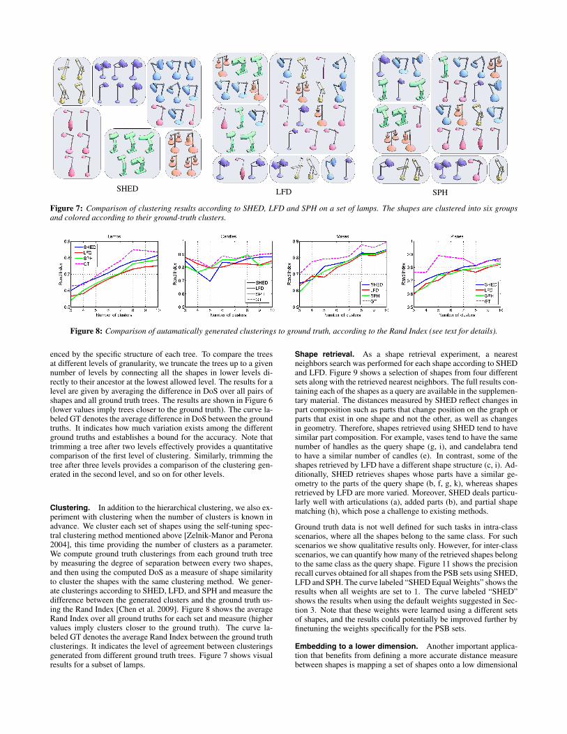
Figure 7: Comparison of clustering results according to SHED, LFD and SPH on a set of lamps. The shapes are clustered into six groupsand colored according to their ground-truth clusters.

Figure 8: Comparison of autamatically generated clusterings to ground truth, according to the Rand Index (see text for details).

enced by the specific structure of each tree. To compare the treesat different levels of granularity, we truncate the trees up to a givennumber of levels by connecting all the shapes in lower levels di-rectly to their ancestor at the lowest allowed level. The results for alevel are given by averaging the difference in DoS over all pairs ofshapes and all ground truth trees. The results are shown in Figure 6(lower values imply trees closer to the ground truth). The curve la-beled GT denotes the average difference in DoS between the groundtruths. It indicates how much variation exists among the differentground truths and establishes a bound for the accuracy. Note thattrimming a tree after two levels effectively provides a quantitativecomparison of the first level of clustering. Similarly, trimming thetree after three levels provides a comparison of the clustering gen-erated in the second level, and so on for other levels.

Clustering. In addition to the hierarchical clustering, we also ex-periment with clustering when the number of clusters is known inadvance. We cluster each set of shapes using the self-tuning spec-tral clustering method mentioned above [Zelnik-Manor and Perona2004], this time providing the number of clusters as a parameter.We compute ground truth clusterings from each ground truth treeby measuring the degree of separation between every two shapes,and then using the computed DoS as a measure of shape similarityto cluster the shapes with the same clustering method. We gener-ate clusterings according to SHED, LFD, and SPH and measure thedifference between the generated clusters and the ground truth us-ing the Rand Index [Chen et al. 2009]. Figure 8 shows the averageRand Index over all ground truths for each set and measure (highervalues imply clusters closer to the ground truth). The curve la-beled GT denotes the average Rand Index between the ground truthclusterings. It indicates the level of agreement between clusteringsgenerated from different ground truth trees. Figure 7 shows visualresults for a subset of lamps.

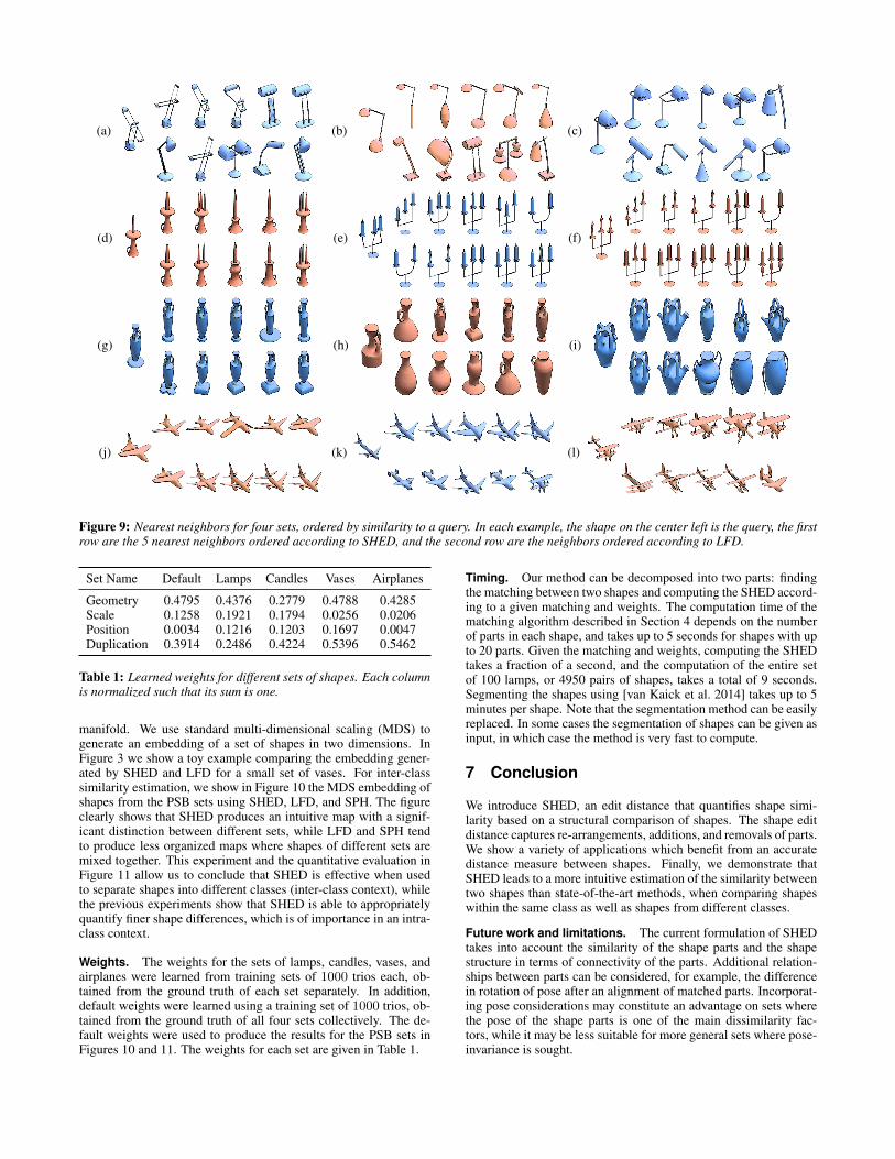
Shape retrieval. As a shape retrieval experiment, a nearestneighbors search was performed for each shape according to SHEDand LFD. Figure 9 shows a selection of shapes from four differentsets along with the retrieved nearest neighbors. The full results con-taining each of the shapes as a query are available in the supplemen-tary material. The distances measured by SHED reflect changes inpart composition such as parts that change position on the graph orparts that exist in one shape and not the other, as well as changesin geometry. Therefore, shapes retrieved using SHED tend to havesimilar part composition. For example, vases tend to have the samenumber of handles as the query shape (g, i), and candelabra tendto have a similar number of candles (e). In contrast, some of theshapes retrieved by LFD have a different shape structure (c, i). Ad-ditionally, SHED retrieves shapes whose parts have a similar ge-ometry to the parts of the query shape (b, f, g, k), whereas shapesretrieved by LFD are more varied. Moreover, SHED deals particu-larly well with articulations (a), added parts (b), and partial shapematching (h), which pose a challenge to existing methods.

Ground truth data is not well defined for such tasks in intra-classscenarios, where all the shapes belong to the same class. For suchscenarios we show qualitative results only. However, for inter-classscenarios, we can quantify how many of the retrieved shapes belongto the same class as the query shape. Figure 11 shows the precisionrecall curves obtained for all shapes from the PSB sets using SHED,LFD and SPH. The curve labeled “SHED Equal Weights” shows theresults when all weights are set to 1. The curve labeled “SHED”shows the results when using the default weights suggested in Sec-tion 3. Note that these weights were learned using a different setsof shapes, and the results could potentially be improved further byfinetuning the weights specifically for the PSB sets.

Embedding to a lower dimension. Another important applica-tion that benefits from defining a more accurate distance measurebetween shapes is mapping a set of shapes onto a low dimensional

(a) (b) (c)

(d) (e) (f)

(g) (h) (i)

(j) (k) (l)

Figure 9: Nearest neighbors for four sets, ordered by similarity to a query. In each example, the shape on the center left is the query, the firstrow are the 5 nearest neighbors ordered according to SHED, and the second row are the neighbors ordered according to LFD.

Set Name Default Lamps Candles Vases Airplanes

Geometry 0.4795 0.4376 0.2779 0.4788 0.4285Scale 0.1258 0.1921 0.1794 0.0256 0.0206Position 0.0034 0.1216 0.1203 0.1697 0.0047Duplication 0.3914 0.2486 0.4224 0.5396 0.5462

Table 1: Learned weights for different sets of shapes. Each columnis normalized such that its sum is one.

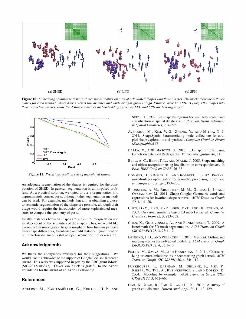
manifold. We use standard multi-dimensional scaling (MDS) togenerate an embedding of a set of shapes in two dimensions. InFigure 3 we show a toy example comparing the embedding gener-ated by SHED and LFD for a small set of vases. For inter-classsimilarity estimation, we show in Figure 10 the MDS embedding ofshapes from the PSB sets using SHED, LFD, and SPH. The figureclearly shows that SHED produces an intuitive map with a signif-icant distinction between different sets, while LFD and SPH tendto produce less organized maps where shapes of different sets aremixed together. This experiment and the quantitative evaluation inFigure 11 allow us to conclude that SHED is effective when usedto separate shapes into different classes (inter-class context), whilethe previous experiments show that SHED is able to appropriatelyquantify finer shape differences, which is of importance in an intra-class context.

Weights. The weights for the sets of lamps, candles, vases, andairplanes were learned from training sets of 1000 trios each, ob-tained from the ground truth of each set separately. In addition,default weights were learned using a training set of 1000 trios, ob-tained from the ground truth of all four sets collectively. The de-fault weights were used to produce the results for the PSB sets inFigures 10 and 11. The weights for each set are given in Table 1.

Timing. Our method can be decomposed into two parts: findingthe matching between two shapes and computing the SHED accord-ing to a given matching and weights. The computation time of thematching algorithm described in Section 4 depends on the numberof parts in each shape, and takes up to 5 seconds for shapes with upto 20 parts. Given the matching and weights, computing the SHEDtakes a fraction of a second, and the computation of the entire setof 100 lamps, or 4950 pairs of shapes, takes a total of 9 seconds.Segmenting the shapes using [van Kaick et al. 2014] takes up to 5minutes per shape. Note that the segmentation method can be easilyreplaced. In some cases the segmentation of shapes can be given asinput, in which case the method is very fast to compute.

7 Conclusion

We introduce SHED, an edit distance that quantifies shape simi-larity based on a structural comparison of shapes. The shape editdistance captures re-arrangements, additions, and removals of parts.We show a variety of applications which benefit from an accuratedistance measure between shapes. Finally, we demonstrate thatSHED leads to a more intuitive estimation of the similarity betweentwo shapes than state-of-the-art methods, when comparing shapeswithin the same class as well as shapes from different classes.

Future work and limitations. The current formulation of SHEDtakes into account the similarity of the shape parts and the shapestructure in terms of connectivity of the parts. Additional relation-ships between parts can be considered, for example, the differencein rotation of pose after an alignment of matched parts. Incorporat-ing pose considerations may constitute an advantage on sets wherethe pose of the shape parts is one of the main dissimilarity fac-tors, while it may be less suitable for more general sets where pose-invariance is sought.

(a) SHED (b) LFD (c) SPH

Figure 10: Embedding obtained with multi-dimensional scaling on a set of articulated shapes with three classes. The insets show the distancematrix for each method, where dark green is low distance and white or light green is high distance. Note how SHED groups the shapes intotheir respective classes, while the distance matrices and embeddings given by LFD and SPH are less organized.

Figure 11: Precision-recall on sets of articulated shapes.

An adequate segmentation of the shapes is required for the com-putation of SHED. In general, segmentation is an ill-posed prob-lem. As a practical solution, we opted to use a segmentation intoapproximately convex parts, although other segmentation methodscan be used. For example, methods that aim at obtaining a close-to-semantic segmentation of the shape are possible, although theirusage would require the introduction of more sophisticated mea-sures to compare the geometry of parts.

Finally, distances between shapes are subject to interpretation andare dependent on the semantics of the shapes. Thus, we would liketo conduct an investigation to gain insight on how humans perceivefiner shape differences, to enhance our edit distance. Quantificationof intra-class distances is still an open avenue for further research.

Acknowledgments

We thank the anonymous reviewers for their suggestions. Wewould like to acknowledge the support of Google Focused ResearchAward. This work was supported in part by the ERC grant iModel(StG-2012-306877). Oliver van Kaick is grateful to the AzrieliFoundation for the award of an Azrieli Fellowship.

References

ANKERST, M., KASTENMULLER, G., KRIEGEL, H.-P., AND

SEIDL, T. 1999. 3D shape histograms for similarity search andclassification in spatial databases. In Proc. Int. Symp. Advancesin Spatial Databases, 207–226.

AVERKIOU, M., KIM, V. G., ZHENG, Y., AND MITRA, N. J.2014. ShapeSynth: Parameterizing model collections for cou-pled shape exploration and synthesis. Computer Graphics Forum(Eurographics) 33.

BARRA, V., AND BIASOTTI, S. 2013. 3D shape retrieval usingkernels on extended Reeb graphs. Pattern Recognition 46, 11.

BERG, A. C., BERG, T. L., AND MALIK, J. 2005. Shape matchingand object recognition using low distortion correspondences. InProc. IEEE Conf. on CVPR, 26–33.

BOMMES, D., ZIMMER, H., AND KOBBELT, L. 2012. Practicalmixed-integer optimization for geometry processing. In Curvesand Surfaces. Springer, 193–206.

BRONSTEIN, A. M., BRONSTEIN, M. M., GUIBAS, L. J., ANDOVSJANIKOV, M. 2011. Shape Google: Geometric words andexpressions for invariant shape retrieval. ACM Trans. on Graph30, 1, 1:1–20.

CHEN, D.-Y., TIAN, X.-P., SHEN, Y.-T., AND OUHYOUNG, M.2003. On visual similarity based 3D model retrieval. ComputerGraphics Forum 22, 3, 223–232.

CHEN, X., GOLOVINSKIY, A., AND FUNKHOUSER, T. 2009. Abenchmark for 3D mesh segmentation. ACM Trans. on Graph(SIGGRAPH) 28, 3, 73:1–12.

DENNING, J. D., AND PELLACINI, F. 2013. MeshGit: Diffing andmerging meshes for polygonal modeling. ACM Trans. on Graph(SIGGRAPH) 32, 4, 35:1–10.

FISHER, M., SAVVA, M., AND HANRAHAN, P. 2011. Character-izing structural relationships in scenes using graph kernels. ACMTrans. on Graph (SIGGRAPH) 30, 4, 34:1–12.

FUNKHOUSER, T., KAZHDAN, M., SHILANE, P., MIN, P.,KIEFER, W., TAL, A., RUSINKIEWICZ, S., AND DOBKIN, D.2004. Modeling by example. ACM Trans. on Graph (SIG-GRAPH) 23, 3, 652–663.

GAO, X., XIAO, B., TAO, D., AND LI, X. 2010. A survey ofgraph edit distance. Pattern Anal. Appl. 13, 1, 113–129.

HARCHAOUI, Z., AND BACH, F. 2007. Image classification withsegmentation graph kernels. In Proc. IEEE Conf. on CVPR, 1–8.

HILAGA, M., SHINAGAWA, Y., KOHMURA, T., AND KUNII, T. L.2001. Topology matching for fully automatic similarity estima-tion of 3D shapes. In Proc.SIGGRAPH, 203–212.

HUANG, Q., KOLTUN, V., AND GUIBAS, L. 2011. Joint shapesegmentation with linear programming. ACM Trans. on Graph(SIGGRAPH Asia) 30, 6, 125:1–12.

HUANG, Q.-X., SU, H., AND GUIBAS, L. 2013. Fine-grainedsemi-supervised labeling of large shape collections. ACM Trans-actions on Graphics (TOG) 32, 6, 190.

HUANG, S.-S., SHAMIR, A., SHEN, C.-H., ZHANG, H., SHEF-FER, A., HU, S.-M., AND COHEN-OR, D. 2013. Qualitativeorganization of collections of shapes via quartet analysis. ACMTrans. on Graph (SIGGRAPH) 32, 4, 71:1–10.

KALOGERAKIS, E., CHAUDHURI, S., KOLLER, D., ANDKOLTUN, V. 2012. A probabilistic model of component-basedshape synthesis. ACM Trans. on Graph (SIGGRAPH) 31, 4,55:1–11.

KAZHDAN, M., FUNKHOUSER, T., AND RUSINKIEWICZ, S.2003. Rotation invariant spherical harmonic representation of3D shape descriptors. In Symp. on Geom. Proc., 156–164.

KEZURER, I., KOVALSKY, S. Z., BASRI, R., AND LIPMAN, Y.2015. Tight relaxation of quadratic matching. Computer Graph-ics Forum 24, 5.

KIM, V. G., LI, W., MITRA, N. J., DIVERDI, S., ANDFUNKHOUSER, T. 2012. Exploring collections of 3D models us-ing fuzzy correspondences. ACM Trans. on Graph (SIGGRAPH)31, 4, 54:1–11.

KIM, V. G., LI, W., MITRA, N. J., CHAUDHURI, S., DIVERDI,S., AND FUNKHOUSER, T. 2013. Learning part-based templatesfrom large collections of 3D shapes. ACM Trans. on Graph (SIG-GRAPH) 32, 4, 70:1–12.

KLEIMAN, Y., FISH, N., LANIR, J., AND COHEN-OR, D. 2013.Dynamic maps for exploring and browsing shapes. ComputerGraphics Forum (SGP) 32, 5, 187–196.

KURTEK, S., SRIVASTAVA, A., KLASSEN, E., AND LAGA, H.2013. Landmark-guided elastic shape analysis of spherically-parameterized surfaces. Computer Graphics Forum 32, 2pt4,429–438.

LAGA, H., MORTARA, M., AND SPAGNUOLO, M. 2013. Geom-etry and context for semantic correspondences and functionalityrecognition in man-made 3D shapes. ACM Trans. on Graph 32,5, 150:1–16.

LEORDEANU, M., AND HEBERT, M. 2005. A spectral techniquefor correspondence problems using pairwise constraints. In Proc.Int. Conf. on Comp. Vis., 1482–1489.

LI, B., GODIL, A., AONO, M., BAI, X., FURUYA, T., LI, L.,LOPEZ-SASTRE, R., JOHAN, H., OHBUCHI, R., REDONDO-CABRERA, C., TATSUMA, A., YANAGIMACHI, T., ANDZHANG, S. 2012. SHREC’12 track: Generic 3D shape retrieval.In Eurographics Workshop on 3D Object Retrieval (3DOR),M. Spagnuolo, M. Bronstein, A. Bronstein, and A. Ferreira, Eds.

LITMAN, R., BRONSTEIN, A., BRONSTEIN, M., AND CASTEL-LANI, U. 2014. Supervised learning of bag-of-features shapedescriptors using sparse coding. Computer Graphics Forum 33,5, 127–136.

LYZINSKI, V., FISHKIND, D., FIORI, M., VOGELSTEIN, J.,PRIEBE, C., AND SAPIRO, G. 2015. Graph matching: relaxat your own risk. IEEE TPAMI.

MITRA, N. J., WAND, M., ZHANG, H., COHEN-OR, D., ANDBOKELOH, M. 2013. Structure-aware shape processing. InProc. Eurographics State-of-the-art Reports.

NEUHAUS, M., AND BUNKE, H. 2007. Bridging the Gap BetweenGraph Edit Distance and Kernel Machines. World Scientific,River Edge, NJ, USA.

OSADA, R., FUNKHOUSER, T., CHAZELLE, B., AND DOBKIN,D. 2002. Shape distributions. ACM Trans. on Graph 21, 4,807–832.

OVSJANIKOV, M., MERIGOT, Q., MEMOLI, F., AND GUIBAS, L.2010. One point isometric matching with the heat kernel. Com-puter Graphics Forum (SGP) 29, 5, 1555–1564.

OVSJANIKOV, M., LI, W., GUIBAS, L., AND MITRA, N. J. 2011.Exploration of continuous variability in collections of 3D shapes.ACM Trans. on Graph (SIGGRAPH) 30, 4, 33:1–10.

RUSTAMOV, R. M. 2007. Laplace-Beltrami eigenfunctions fordeformation invariant shape representation. In Symp. on Geom.Proc., 225–233.

SCHULTZ, M., AND JOACHIMS, T. 2004. Learning a distance met-ric from relative comparisons. Advances in neural informationprocessing systems (NIPS), 41.

SEBASTIAN, T., KLEIN, P., AND KIMIA, B. 2004. Recognitionof shapes by editing their shock graphs. IEEE Trans. Pat. Ana.& Mach. Int. 26, 5, 550–571.

SHAMIR, A. 2008. A survey on mesh segmentation techniques.Computer Graphics Forum 27, 6, 1539–1556.

SHAPIRA, L., SHAMIR, A., AND COHEN-OR, D. 2008. Consis-tent mesh partitioning and skeletonisation using the shape diam-eter function. The Visual Computer 24, 4, 249–259.

SIDI, O., VAN KAICK, O., KLEIMAN, Y., ZHANG, H., ANDCOHEN-OR, D. 2011. Unsupervised co-segmentation of a setof shapes via descriptor-space spectral clustering. ACM Trans.on Graph (SIGGRAPH Asia) 30, 6, 126:1–10.

SUNDAR, H., SILVER, D., GAGVANI, N., AND DICKINSON, S.2003. Skeleton based shape matching and retrieval. In ShapeModeling International, 130–139.

TANGELDER, J. W. H., AND VELTKAMP, R. C. 2008. A surveyof content based 3D shape retrieval methods. Multimedia Toolsand Applications 39, 3, 441–471.

VAN KAICK, O., FISH, N., KLEIMAN, Y., ASAFI, S., ANDCOHEN-OR, D. 2014. Shape segmentation by approximate con-vexity analysis. ACM Trans. Graph. 34, 1, 4:1–11.

WANG, Y., ASAFI, S., VAN KAICK, O., ZHANG, H., COHEN-OR,D., AND CHEN, B. 2012. Active co-analysis of a set of shapes.ACM Trans. on Graph (SIGGRAPH Asia) 31, 6, 157:1–10.

XU, K., LI, H., ZHANG, H., COHEN-OR, D., XIONG, Y., ANDCHENG, Z. 2010. Style-content separation by anisotropic partscales. ACM Trans. on Graph (SIGGRAPH Asia) 29, 6.

ZELNIK-MANOR, L., AND PERONA, P. 2004. Self-tuning spectralclustering. In NIPS, vol. 17, 1601–1608.

ZHENG, Y., COHEN-OR, D., AVERKIOU, M., AND MITRA, N. J.2014. Recurring part arrangements in shape collections. Com-puter Graphics Forum (Eurographics) 33.