Embed Size (px)
Citation preview

Shear Wave Seismic Study Comparing 9C3D SV and SH Images with 3C3D C-Wave Images
FINAL REPORT
Reporting Period Start Date: January 1, 2003
Reporting Period End Date: June 30, 2004
John Beecherl, Principal Investigator* Bob A. Hardage**
July 2004
Work performed under DOE Grant DE-FG26-03NT15431
Prepared by
*Vecta Technology
5950 Cedar Springs Road, Suite 225 Dallas, TX 75235
and
**Bureau of Economic Geology
John A. and Katherine G. Jackson School of Geosciences The University of Texas at Austin
University Station, P.O. Box X Austin, TX 78713-8924

ii
DISCLAIMER
This report was prepared as an account of work sponsored by an agency of the United States Government. Neither the United States Government nor any agency thereof, nor any of their employees, makes any warranty, express or implied, or assumes any legal liability for responsibility for the accuracy, completeness, or usefulness of any information, apparatus, product, or process disclosed, or represents that its use would not infringe privately owned rights. Reference herein to any specific commercial product, process, or service by trade name, trademark, manufacturer, or otherwise does not necessarily constitute or imply its endorsement, recommendation, or favoring by the United States Government or any agency thereof. The views and opinions of authors expressed herein do not necessarily state or reflect those of the United States Government or any agency thereof.

iii
ABSTRACT The objective of this study was to compare the relative merits of shear-wave (S-
wave) seismic data acquired with nine-component (9-C) technology and with three-component (3-C) technology. The original proposal was written as if the investigation would be restricted to a single 9-C seismic survey in southwest Kansas (the Ashland survey), on the basis of the assumption that both 9-C and 3-C S-wave images could be created from that one data set. The Ashland survey was designed as a 9-C seismic program. We found that although the acquisition geometry was adequate for 9-C data analysis, the source-receiver geometry did not allow 3-C data to be extracted on an equitable and competitive basis with 9-C data. To do a fair assessment of the relative value of 9-C and 3-C seismic S-wave data, we expanded the study beyond the Ashland survey and included multicomponent seismic data from surveys done in a variety of basins. These additional data were made available through the Bureau of Economic Geology, our research subcontractor.
Bureau scientists have added theoretical analyses to this report that provide valuable insights into several key distinctions between 9-C and 3-C seismic data. These theoretical considerations about distinctions between 3-C and 9-C S-wave data are presented first, followed by a discussion of differences between processing 9-C common-midpoint data and 3-C common-conversion-point data. Examples of 9-C and 3-C data are illustrated and discussed in the last part of the report.
The key findings of this study are that each S-wave mode (SH-SH, SV-SV, or P-SV) involves a different subsurface illumination pattern and a different reflectivity behavior and that each mode senses a different Earth fabric along its propagation path because of the unique orientation of its particle-displacement vector. As a result of the distinct orientation of each mode’s particle-displacement vector, one mode may react to a critical geologic condition in a more optimal way than do the other modes. A conclusion of the study is that 9-C seismic data contain more rock and fluid information and more sequence and facies information than do 3-C seismic data; 9-C data should therefore be acquired in multicomponent seismic programs whenever possible.

iv
CONTENTS
Abstract ..................................................................................................................... iii
Introduction .................................................................................................................1
Executive Summary ....................................................................................................2
Basic Concepts That Distinguish 9-C and 3-C S-Wave Data .....................................3
Concept 1: Vector-Based Technology ...................................................................4
Concept 2: Components of Multicomponent Seismic Data.................................10
Argument 1: Sensing the Earth Fabric .................................................................12
Terminology.........................................................................................................13
Marine Environments ..........................................................................................15
Argument 2: Multicomponent Reflectivities .......................................................17
Argument 3: Multicomponent Illumination .........................................................26
Elastic-Wavefield Seismic Stratigraphy ..............................................................33
Data-Processing Differences between 9-C and 3-C S-Wave Data ...........................36
Common-Midpoint (CMP) Imaging ....................................................................36
Common-Conversion-Point (CCP) Imaging........................................................37
CMP and CCP Velocity Analyses .......................................................................40
CMP and CCP Stacking .......................................................................................43
Examples of 9-C and 3-C S-Wave Data ...................................................................49
Distinctions between SH-SH and SV-SV S-Wave Modes ..................................50
3-C Data Polarizations .........................................................................................55
Making 3-C and 9-C Images Depth Equivalent ...................................................61

v
Conclusions ...............................................................................................................62
References .................................................................................................................64
Figures
1. Distinction between vector and scalar seismic sources ...................................................5
2. An example of three orthogonal seismic vector sources working to produce nine-component vertical seismic profile data ..............................................................................7
3. Twelve vector sources ready to deploy across a large 9C3D seismic survey ..................7
4. Standard three-component moving-coil geophone ..........................................................8
5. Micro-Electro-Mechanical System three-component seismic sensor available from Input/Output .........................................................................................................................9
6. MEMS three-component sensor package available from Sercel ...................................10
7. Full-elastic, multicomponent seismic wavefield propagating in a homogeneous Earth consisting of a compressional mode P and two shear modes, SV and SH ........................11
8. Distinction between SH and SV shear wave displacements ..........................................12
9. Options for acquiring multicomponent seismic data and seismic modes associated with each option .........................................................................................................................15
10. One type of multicomponent seismic sensor that can be deployed on the seafloor to record multicomponent marine seismic data .....................................................................16
11. Reflectivity equation for the SH-SH seismic mode .....................................................19
12. Analysis of P and SV reflectivities requires that a polarity convention be assumed for the particle-displacement vectors .......................................................................................20
13. Each incident P and SV mode creates four scattered modes at an interface ................20
14. Mathematical terms needed for P and SV reflectivity equations .................................21
15. Reflectivity equations for downgoing P-mode illumination ........................................22
16. Reflectivity equations for downgoing SV-mode illumination .....................................22
17. Side-by-side comparison of 3-C and 9-C reflectivity equations ..................................23

vi
18. Simplified formulation for P-wave reflectivity that can be used when two elastic media at an interface have “similar” petrophysical properties ..........................................25
19. Simplified formulation for SV reflectivity that can be used when two elastic media at an interface have “similar” petrophysical properties .........................................................25
20. Map view of particle-displacement wavefield propagating away from a horizontal-displacement vector source ................................................................................................27
21. Map view of SH and SV illumination patterns for orthogonal horizontal-displacement sources................................................................................................................................29
22. Section view of P-SV radiation pattern .......................................................................30
23. Map view of P-SV illumination pattern .......................................................................31
24. Side-by-side comparison of 3-C and 9-C S-wave illumination patterns .....................32
25. Distinctions between 3-C SV-mode polarization and 9-C SV-mode polarization ......33
26. Distinction between 9-C CMP image points and 3-C CCP image points .................. 37
27. Distinction between 3-C CCP image coordinates and 9-C CMP image point coordinates ........................................................................................................................ 39
28. Distinction between a 9-C SV-P CCP raypath and a 3-C P-SV CCP raypath ............ 40
29. Traveltimes for positive offsets are the same as traveltimes for negative offsets in 9-C CMP imaging because the lengths of the travel paths in Facies 1 and 2 are the same for both offset options..............................................................................................................41
30. Traveltimes for positive offsets are not the same as traveltimes for negative offsets in 3-C CCP imaging because the lengths of the P and SV raypaths in Facies 1 and 2 change when the offset direction changes ......................................................................................42
31. Comparison of 9-C CMP image trace and 3-C CCP image trace ................................44
32. Single vertical image trace in one stacking bin of CCP image space must be constructed by summing data from different time windows of all CCP traces that traverse the bin.................................................................................................................................46
33. Simple, straight-raypath model showing that the velocity ratio Vp/Vs in the propagation medium controls the position of a 3-C P-SV image coordinate in seismic image space ........................................................................................................................47
34. 9-C SV-SV and SH-SH super gathers shown in field-record format ..........................51

vii
35. 9-C SV-SV and SH-SH trace gathers after processing to emphasize primary reflections between 2 and 2.5 s ..........................................................................................53
36. Wave mode velocities calculated for transverse isotropic media showing that 9-C SV and SH velocities differ in a flat-layered Earth .................................................................54
37. Example 1 of polarities of 3-C P-SV data measured in azimuth directions that differ by 180° ...............................................................................................................................56
38. Example 2 of polarities of 3-C P-SV data measured in azimuth directions that differ by 180° ...............................................................................................................................58
39. 2-D field record showing polarity behavior of the inline-horizontal component of P-SV data .............................................................................................................................. 60

1
INTRODUCTION Several concepts involved in generating, acquiring, and processing
multicomponent seismic data are essential for understanding distinctions between 9-
component (9-C) and 3-component (3-C) data. The basic principle that has to be
emphasized is that the physics of any multicomponent seismic technology cannot be
understood until the data are viewed in terms of the displacement vector associated with
each mode of the seismic wavefield that is being considered. This report therefore begins
with a discussion of seismic vector-wavefield behavior to set the stage for all subsequent
discussions.
There are three arguments that can be used to explain why each S-wave mode of
9-C and 3-C seismic data carries a different amount and a different type of rock/fluid
information. These arguments were developed by scientists subcontracted to this study at
the Bureau of Economic Geology (Bureau). One argument is designed to appeal to people
who have limited interest in mathematics. The second approach is structured for people
who have an appreciation of the mathematics of wavefield reflectivity. The third option is
to illustrate the fundamental differences in the S-wave radiation patterns and S-wave
target illuminations associated with 9-C and 3-C seismic sources.

2
EXECUTIVE SUMMARY
This investigation summarizes the basic physics of nine-component (9-C) and
three-component (3-C) shear-wave (S-wave) data and illustrates selected physical
concepts of 9-C and 3-C S-waves with real data examples. There are fundamental
differences in the P-SV S-wave mode provided by 3-C seismic data and the SH-SH and
SV-SV S-wave modes available with 9-C data. Key distinctions among these S-wave
modes are explained by describing differences in the sources that generate the modes,
illustrating how the downgoing wavefields of the modes result in different illuminations
of a target, showing differences in the reflectivity behaviors of the modes, and stressing
how different source-receiver geometries and different data-processing strategies are
required for 9-C data and for 3-C data. A principle that is stressed and illustrated
repeatedly is that each mode of a multicomponent seismic wavefield may sense a
different Earth fabric along its propagation path because the particle-displacement vector
of each mode is oriented in a different direction. We conclude that because each wave
mode has the potential of sensing an Earth fabric that its companion modes cannot, that
optimal seismic evaluation of hydrocarbon prospects can occur only when 9-C seismic
data are acquired. 9-C seismic data provide all possible wave modes and all possible
fabric-sensing options. 3-C seismic data provide only two fabric-sensing options: the P-P
mode and the P-SV mode.

3
BASIC CONCEPTS THAT DISTINGUISH 9-C AND 3-C S-WAVE DATA
The nonmathematical approach used to distinguish 9-C and 3-C S-wave data will
be considered first. The logic of this argument emphasizes how differently Earth fabric
can be sensed when a small rock volume embedded in a layered, spatially variant Earth is
deformed in a different direction by the orthogonal displacement vectors associated with
various seismic wave modes. Estimation of Earth fabric obtained from individual seismic
wave modes can differ, and yet each estimate can be correct, because each mode deforms
the test volume of rock in a different direction. These deformations sense different Earth
resistance in directions parallel to, and normal to, various symmetry planes in real-Earth
media. The logic of this nonmathematical model appeals in particular to people who are
interested in only the geologic and petrophysical information that multicomponent
seismic data may provide.
The second approach used to distinguish 9-C and 3-C wavefield behavior focuses
on the mathematics of the reflectivity equation associated with each mode of the full-
elastic seismic wavefield. The mathematical structure of the reflectivity equation
associated with each seismic wave mode describes why and how petrophysical properties
of the propagation medium affect different wave modes in different ways. The logic of
this model is appreciated by geophysicists, engineers, and others who are comfortable
with mathematics.
The third and last argument used to emphasize differences in 9-C and 3-C seismic
data focuses on the S-wave illumination patterns produced by 9-C and 3-C seismic
sources. The physics of the S-wave radiation associated with these sources is explained

4
graphically, not numerically, to again have greater appeal to that large community of
multicomponent seismic users who prefer not to be burdened by mathematical analyses.
All of these concepts led to the development of a new seismic interpretation
science called elastic-wavefield seismic stratigraphy, which will be briefly described. The
fundamental principle of elastic-wavefield seismic stratigraphy is that any mode of the
elastic wavefield may provide unique rock, fluid, or sequence information across some
stratigraphic intervals that cannot be obtained with the other wave modes of the elastic
wavefield.
Concept 1: Vector-Based Technology
A special thought process based on vector concepts has to be used when
developing and applying multicomponent seismic technology, regardless of whether the
effort involves 9-C data or 3-C data. Previous seismic technology has been scalar based.
For scalar data, it is not necessary to know the direction that each seismic wave mode
moves the Earth. In multicomponent seismic technology, it is mandatory to know the
direction of Earth displacement (vector-based thinking) when any step is taken to create,
process, or interpret multicomponent data.
If the objective is to conduct a multicomponent seismic survey that will produce
all possible wave modes, then each source station must be occupied by sources that
generate three orthogonal source-displacement vectors. These three vectors must then
propagate through the Earth as three independent illuminating wavefields. Such sources
are called vector sources (Fig. 1). Full-vector source illumination requires that one
illuminating wavefield (designated as wavefront 1) has a displacement vector oriented

5
normal to its wavefront, and that two illuminating wavefields (designated as wavefronts 2
and 3) have orthogonal displacement vectors that are tangent to the respective wavefronts
(Fig. 1). The displacement vector that is normal to wavefront 1 generates compressional
(P-wave) data. The displacement vectors that are tangent to wavefronts 2 and 3 create
shear (S-wave) data.
Figure 1. Distinction between vector and scalar seismic sources. A full-vector vector source should cause three orthogonal displacement vectors to propagate through the Earth. Two seismic properties are measured for a vector seismic source: the time-varying magnitude and the time-varying direction of the displacement of the Earth. A scalar source creates at least one displacement vector, but the seismic property that is measured is only the time-varying change of the magnitude of Earth movement, not the direction of that movement.

6
An example of three vector-based vibrator sources positioned to create orthogonal
source-displacement vectors is shown in Figure 2. In this example, a single vibrator is
used to produce each of the three orthogonal source-displacement vectors illustrated for a
vector source in Figure 1. A single-vibrator source is satisfactory in this instance because
the data being acquired are 9-C vertical seismic profile (VSP) data, which do not require
extreme, robust sources to produce good data quality. In large-scale 3-D seismic
programs, arrays of vibrators may be needed to produce good-quality source-
displacement vectors at large offset distances. An example of 12 vibrators assembled for
a 9C3D seismic survey is shown in Figure 3. In this instance, an array of four vertical
vibrators produced the vertical-displacement source vector, an array of four horizontal
vibrators produced the inline horizontal-displacement source vector, and a second array
of four horizontal vibrators produced the crossline horizontal-displacement source vector.
If the sources do not create these three orthogonal source-displacement vectors, some
seismic wave modes of the full-elastic wavefield will not propagate into the Earth. The
illuminating wavefields associated with the three orthogonal displacement vectors are
produced and recorded in a time-sequence manner, with time delays of minutes to hours
between generation of the vertical displacement vector, the inline horizontal-
displacement vector, and the crossline horizontal-displacement vector at each source
station.

7
Figure 2. An example of three orthogonal seismic vector sources working to produce nine-component vertical seismic profile data. These three vibrators create the three source-displacement vectors illustrated for a vector seismic source in Figure 1 in a time-sequence manner, not simultaneously.
Figure 3. Twelve vector sources ready to deploy across a large 9C3D seismic survey. In this instance, four vibrators work as an array to produce a vertical source-displacement vector; four vibrators work in an array to produce an inline horizontal source-displacement vector; and four vibrators work in an array to produce a crossline horizontal source-displacement vector. These three source-displacement vectors are produced in a time-sequence manner, not simultaneously, at each source station.

8
Equally important, if there are not three orthogonal vector sensors at all receiver
stations, then some wave modes produced by these three orthogonal source-displacement
vectors will not be recorded. Three-component geophones are the oldest and most
common type of vector sensor used to acquire multicomponent seismic data across
onshore seismic prospects. A typical 3-C geophone is illustrated in Figure 4. This sensor
package has one vertical moving-coil geophone element and two orthogonal and
horizontal, moving-coil elements. A second vector-sensor technology based on solid-state
accelerometers is now available and is being used in more and more multicomponent
surveys. These sensors are called Micro-Electro-Mechanical System (MEMS) devices.
The MEMS technology developed by Input/Output is illustrated in Figure 5. Sercel also
offers MEMS 3-C vector sensors. Sercel’s concept for packaging MEMS vector-based
sensors is illustrated in Figure 6.
Figure 4. Standard three-component moving-coil geophone.

9
Figure 5. Micro-Electro-Mechanical System (MEMS) three-component seismic sensor available from Input/Output. The basic sensor element is a solid-state accelerometer.

10
Figure 6. MEMS three-component sensor package available from Sercel.
If each source station is occupied by sources that create three orthogonal source-
displacement vectors (typically three different sources) and the wavefield produced by
each source is then recorded by 3-C vector-based sensors, the result is a 9-C seismic
vector wavefield. If the source station is occupied by a source that generates only one
source-displacement vector (for example, sources such as a vertical vibrator or an
explosive in a shothole in an onshore environment, or an air gun in a marine
environment) and that single wavefield is then recorded by 3-C vector-based sensors, the
result is a 3-C seismic wavefield. Distinctions between 9-C seismic wave modes and 3-C
seismic wave modes will be emphasized throughout this report.
Concept 2: Components That Make Multicomponent Seismic Data
Three independent, vector-based, seismic wave modes propagate in a simple
homogeneous Earth: a compressional mode, P, and two shear modes, SV and SH (Fig.7).
These are the three modes we try to create with three orthogonal source-displacement
vectors and then record with three orthogonal vector sensors. Each mode travels through

11
the Earth at a different velocity, and each mode distorts the Earth in a different direction
as it propagates. The propagation velocities of the SH and SV shear modes differ by only
a few percent, but both shear velocities (Vs) are significantly less than the P-wave
velocity (Vp). The velocity ratio Vp/Vs can vary by an order of magnitude in Earth
media, from a value of 15 in deep-water, unconsolidated, seafloor sediment to a value of
1.5 in a few dense, well-consolidated rocks. The orientations of the P, SV, and SH
displacement vectors relative to the propagation direction of each mode are defined in
Figure 7. A convenient way to distinguish between SH and SV shear modes is to imagine
a vertical plane passing through a source station and a receiver station. SV vector
displacement occurs in this vertical plane; SH vector displacement is normal to the plane
(Fig. 8).
Figure 7. Full-elastic, multicomponent seismic wavefield propagating in a homogeneous Earth consisting of a compressional mode P and two shear modes, SV and SH. A key distinction among these modes is that each mode distorts the Earth in a different direction along its propagation path. The direction in which each mode distorts the Earth is indicated by the double-headed arrows.

12
Figure 8. Distinction between SH and SV shear wave displacements. SV displacement occurs in the vertical plane that passes through the source station and the observation point; SH displacement is normal to this plane.
Argument 1: Sensing the Earth Fabric
We discuss now the first argument that can be used to distinguish how 9-C and 3-
C S-wave data sense petrophysical properties of the seismic propagation medium. This
argument is based on the concept that the Earth’s fabric is a direction-dependent quantity.
In real Earth media, the physical character and elastic properties of the internal
fabric of a small Earth volume depend on the direction in which the internal fabric of that
volume is tested. Different elastic constants (fabric) are sensed when the Earth is
distorted perpendicular to its bedding planes versus being displaced parallel to these
planes, or when the Earth is displaced perpendicular to fractures versus parallel to
fractures. For decades, the only seismic data used in oil and gas applications have been P-
wave (scalar) data. The particle-displacement vector of a P-wave mode senses the Earth
fabric in only one direction—the direction in which the P mode is propagating (Fig. 7).

13
The advantage of multicomponent seismic data is that P, SH, and SV wave modes
sense the Earth’s fabric in three orthogonal directions (Fig. 7). Each wave mode thus
carries unique Earth-fabric information, such as directional-dependent information about
elastic constants, cementation quality, pore geometry, anisotropy axes, and lateral
variations in rock and fluid types, as it leaves a target interval and travels to receiver
stations. The technology challenges are to preserve this increased amount of geologic
information when processing multicomponent seismic data and then to correctly interpret
the geologic messages contained in the P, SH, and SV data volumes that are created.
Terminology
A new vocabulary is required to discuss multicomponent seismic technology. As
previously stated, if three orthogonal source-displacement vectors are created at a source
station (Figs. 2 and 3) and three orthogonal vector sensors record the distinct wavefields
associated with each of these source displacements (Figs. 4 through 6), the result is nine-
component data. Nine-component seismic data contain all possible wave modes. In this
discussion, these wave modes will be designated as P-P, SH-SH, SV-SV, P-SV, and SV-
P. In this nomenclature, the term preceding the hyphen defines the downgoing wavefield,
and the term following the hyphen specifies the upgoing wavefield. Three-component (3-
C) data are generated when three orthogonal vector sensors occupy the receiver stations
but only a P-wave (1-C, or single displacement) source is used to generate the
illuminating wavefield. Only two wave modes are provided by 3-C data: the P-P mode
and the P-SV mode.

14
A shear wave that propagates in an Earth that has vertical fractures, or that has a
consistent tectonic orientation of the maximum horizontal stress vector, will segregate
into two daughter modes called the fast-S mode and the slow-S mode. These daughter
modes travel at different velocities, as their names imply, and they have orthogonal, not
parallel, displacement vectors. The displacement vector of the fast-S mode is oriented
parallel to the symmetry plane that is parallel to the vertical fractures (or parallel to the
maximum horizontal stress if a stress condition is used to describe the propagation
medium). The displacement vector of the slow-S mode is oriented normal to this
symmetry plane. This wave physics is mentioned here only to complete this discussion of
“terminology.” Examples of fast-S and slow-S data will not be included in this report.
The various options for acquiring multicomponent seismic data and the specific
wave modes that are associated with each acquisition option are tabulated in Figure 9.
Note how many S-wave modes are involved in multicomponent seismic data, particularly
in fractured Earth media where S-wave splitting occurs. One terminology error
encountered in multicomponent seismic applications is that people sometimes use the
term “shear wave” and do not specify which particular shear mode is being considered.
Each shear mode listed in Figure 9 is unique and commonly provides geologic
information not available in its companion shear modes. Accurate terminology requires
that we define the specific shear mode(s) we are dealing with in any multicomponent
seismic operation.

15
Figure 9. Options for acquiring multicomponent seismic data and seismic modes associated with each option. The top list applies to an isotropic Earth. The bottom list applies to an anisotropic medium in which S-wave splitting occurs. Subscript 1 defines a fast-S mode; subscript 2 indicates a slow-S mode.
In fact, our use of correct terminology matured during this investigation. For
example, because the terms “SV,” “SH,” and “C-wave” were used in the title of the
proposal that was submitted to DOE, those terms are used in the title of this report. We
would now replace those terms, respectively, with the more accurate nomenclature “SV-
SV,” “SH-SH,” and “P-SV.”
Marine Environments
Shear waves cannot propagate in fluids, or in any media in which the shear
modulus, µ, has a value of zero. For multicomponent seismic data to be acquired in
marine environments, sources and receivers need to be on the seafloor where they are in
contact with sediment that has a nonzero value of µ. To date, no vector-based sources
function efficiently on the seafloor. The only source option for marine seismic data

16
acquisition is an air-gun array suspended or towed in the water column. Such air-gun
sources will produce only P-wave (scalar) seismic wavefields in their water medium.
Because the illuminating wavefield in a marine environment is limited to the P (scalar)
mode, the only scattered wavefields that can be recorded are the P-P mode and the P-SV
mode.
Several types of multicomponent, vector-based sensors can be deployed on the
seafloor. One popular option is illustrated in Figure 10. As shown in this illustration,
marine seafloor sensors contain three orthogonal, vector-sensing geophones, as well as a
scalar-sensing hydrophone. Marine multicomponent seismic data are called four-
component data because the three components of geophone data are combined with the
pressure data (scalar data) provided by the hydrophone. The fourth data component,
pressure, is important because water-column multiples can be better suppressed by
combining the vertical geophone response and hydrophone response.
Figure 10. One type of multicomponent seismic sensor that can be deployed on the seafloor to record multicomponent marine seismic data.

17
Argument 2: Multicomponent Reflectivities
We now move to the second argument that will be used to distinguish 9-C and 3-
C S-wave modes. This argument focuses on the reflectivity equations of multicomponent
wave modes and involves some mathematics.
Each wave mode listed in Figure 9 has a unique reflectivity equation that relates
the reflection amplitude and phase of that mode to elastic impedances of the Earth. These
differing reflectivity equations are often the most compelling evidence to convince
physicists, mathematicians, geophysicists, and other mathematically oriented
investigators that elastic-wavefield seismic stratigraphy is built on a sound premise and
that different Earth fabric is often sensed by each vector of the three orthogonal particle-
displacement vectors involved in multicomponent seismic imaging.
Developing expressions for reflectivity equations of the various modes of a
multicomponent seismic wavefield involves cumbersome and tedious algebra. The
mathematics of reflectivity calculations is not particularly complex because it is
essentially basic trigonometry and algebra. Yet many published analyses of reflectivity
equations contain errors because the equations are lengthy, contain many terms, involve
numerous petrophysical parameters, and provide multiple opportunities for making
simple blunders, such as writing cosine when sine should be used, forgetting to include a
parameter in an expression, inadvertently altering the algebraic sign of a term, or writing
an incorrect subscript on parameters. Some of these published errors have persisted in the
literature for years.
Because these types of errors are easy to make when reflectivity equations are
calculated, most researchers copy the equations from a source that has proven over time

18
to be error free. That approach will be followed in this discussion, using the widely
accepted reflectivity equations published by Aki and Richards (1980).
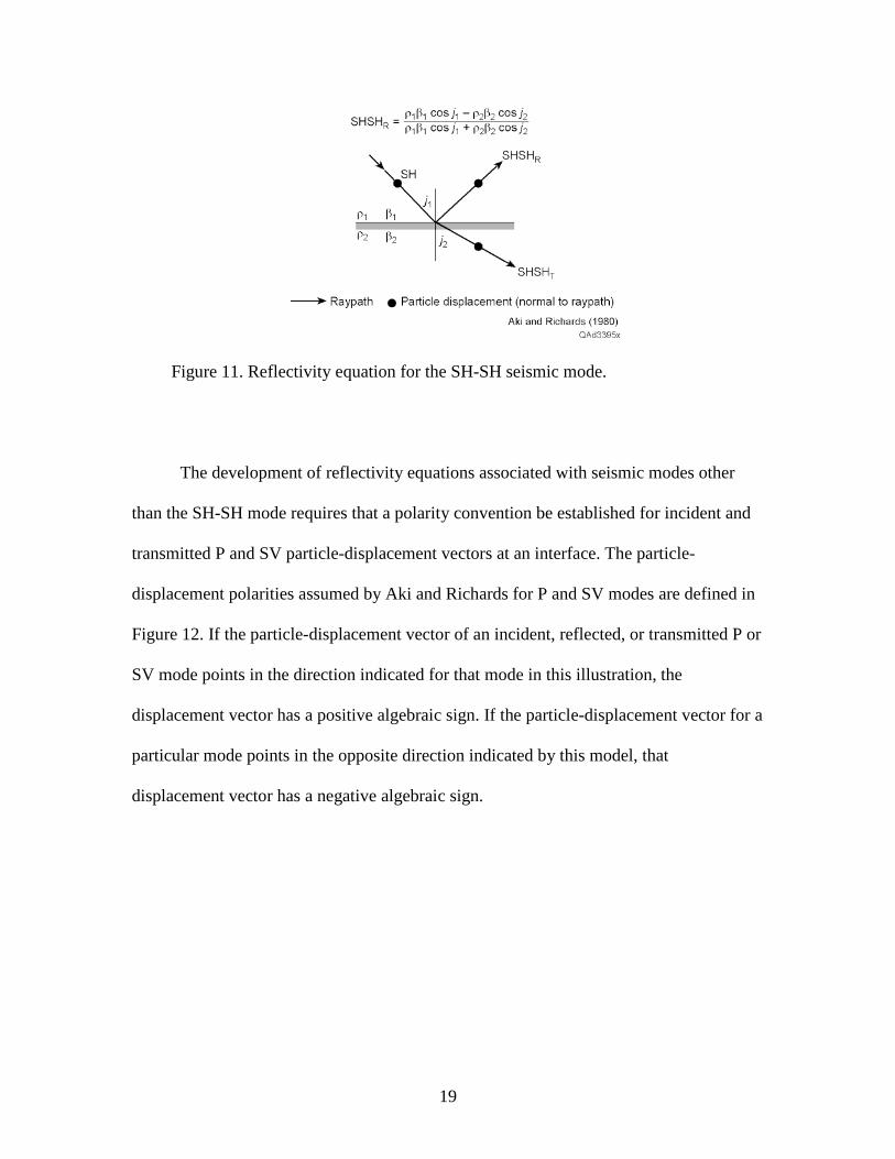
A distinct reflectivity equation is needed for each of the wave modes listed in
Figure 9. The simplest reflectivity equation is the one associated with the SH-SH mode,
which is defined in Figure 11. Also shown in the figure is an illustration of the single-
interface Earth model that will be used in the derivation of all reflectivity equations. This
model and the SH-SH reflectivity equation incorporate the notation for petrophysical
properties used by Aki and Richards (1980). In Aki and Richard’s nomenclature, alpha
and beta represent P-wave and S-wave velocities, respectively. The terms Vp and Vs are
used for these quantities in all other parts of this report. Additional petrophysical
parameters are bulk density (rho), P-wave angle (i), S-wave angle (j), and horizontal
slowness (p). Horizontal slowness is defined as
p = sin(i)/Vp = sin(j)/Vs. (1)
Snell’s law requires the horizontal slowness of every reflected and transmitted
mode to be identical to the horizontal slowness of the incident wave that caused the
reflection and transmission. Indices 1 and 2 attached to parameters refer, respectively, to
the layer above the interface and to the layer below the interface. In Figure 11 and
subsequent figures, subscripts R and T refer, respectively, to reflected and transmitted
modes. The notation for these scattered SH modes is the same as the nomenclature used
in Figure 9, except the hyphen is omitted.
19
Figure 11. Reflectivity equation for the SH-SH seismic mode.
The development of reflectivity equations associated with seismic modes other
than the SH-SH mode requires that a polarity convention be established for incident and
transmitted P and SV particle-displacement vectors at an interface. The particle-
displacement polarities assumed by Aki and Richards for P and SV modes are defined in
Figure 12. If the particle-displacement vector of an incident, reflected, or transmitted P or
SV mode points in the direction indicated for that mode in this illustration, the
displacement vector has a positive algebraic sign. If the particle-displacement vector for a
particular mode points in the opposite direction indicated by this model, that
displacement vector has a negative algebraic sign.
20
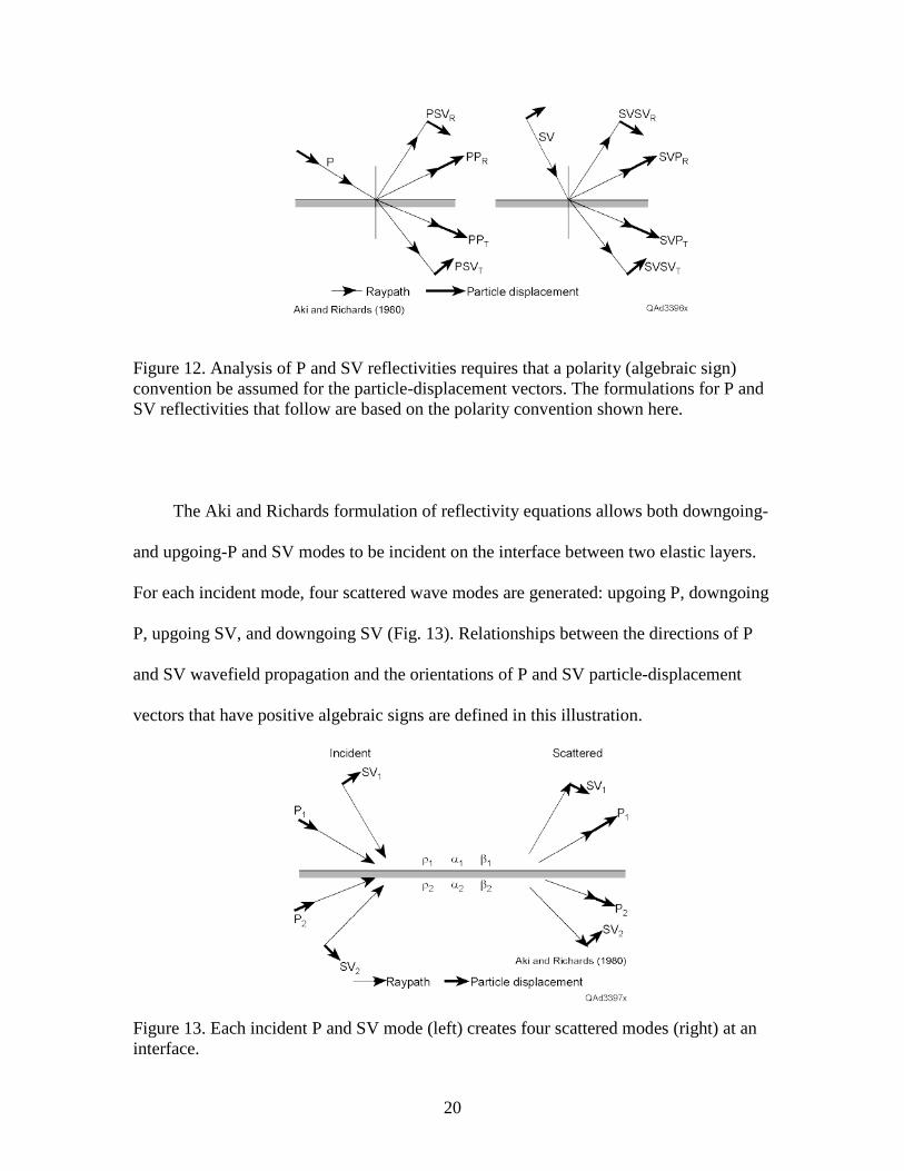
Figure 12. Analysis of P and SV reflectivities requires that a polarity (algebraic sign) convention be assumed for the particle-displacement vectors. The formulations for P and SV reflectivities that follow are based on the polarity convention shown here.
The Aki and Richards formulation of reflectivity equations allows both downgoing-
and upgoing-P and SV modes to be incident on the interface between two elastic layers.
For each incident mode, four scattered wave modes are generated: upgoing P, downgoing
P, upgoing SV, and downgoing SV (Fig. 13). Relationships between the directions of P
and SV wavefield propagation and the orientations of P and SV particle-displacement
vectors that have positive algebraic signs are defined in this illustration.
Figure 13. Each incident P and SV mode (left) creates four scattered modes (right) at an interface.

21
By allowing four scattered modes for each of the four incident modes, Aki and
Richards (1980) developed 16 equations to describe the total reflection/transmission
physics of P and SV wavefields at an interface. Only 4 of these 16 equations are of
interest in this discussion—the two reflectivity equations associated with a downgoing-P
mode and the two reflectivity equations resulting from a downgoing-SV mode. To
shorten the mathematical description of the reflectivity equations, Aki and Richards
introduced the nine terms listed in Figure 14. With these terms being used, the reflectivity
equations associated with a downgoing-P-mode illumination wavefield are then defined
in Figure 15, and the two reflectivity equations produced by a downgoing-SV-mode
illumination wavefield are given in Figure 16.
Figure 14. Mathematical terms needed for P and SV reflectivity equations.

22
Figure 15. Reflectivity equations for downgoing P-mode illumination. These two reflectivity equations are the ones of interest in 3-C and 4-C seismic imaging. Terms a, b, c, d, D, F, and H are defined in Figure 14. Horizontal slowness is defined by Equation 1 in the text. Note how complicated these expressions are compared with the reflectivity equation for the SH mode in Figure 11.
Figure 16. Reflectivity equations for downgoing SV-mode illumination. Terms a, b, c, d, D, E, and H are defined in Figure 14. Horizontal slowness is defined by Equation 1 in the text. Compare the complexity of these expressions with the simpler expression for the reflectivity equation of the SH mode in Figure 11.
All wave modes listed in Figures 15 and 16 have a subscript R because we are
interested in only reflected wavefields in this discussion. The notation used to identify
these reflected modes is identical to the nomenclature in Figure 13 and in Figure 9 (with
the hyphen omitted). The reflectivity equations in Figure 15 are of particular interest
because they describe the P-P and P-SV modes involved in 3-C and 4-C seismic
technology (Fig. 9).

23
Any downgoing-wave mode could be used to acquire 3-C seismic data, but in this
report, 3-C and 4-C seismic technology will be restricted to data produced by only P-
wave illumination. This definition of 3-C and 4-C seismic data is standard practice in the
seismic industry. The reflectivity equations in Figures 11 and 16 thus apply to 9-C
seismic technology, not 3-C seismic technology, because they are produced, respectively,
by SH-mode and SV-mode illumination, not by P-mode illumination. To simplify the
comparison of the reflectivity physics associated with each 3-C and 9-C seismic mode,
the foregoing equations are positioned in a side-by-side format in Figure 17. The left
column describes 3-C (or 4-C) reflectivity. The right column describes 9-C reflectivity.
Figure 17. Side-by-side comparison of 3-C and 9-C reflectivity equations.
Key principles illustrated by these equations can now be noted.
1. 3-C seismic data are a subset of 9-C seismic data (P-P and P-SV modes: top box of both columns).

24
2. Only one S-wave mode (P-SV) is provided by 3-C data; 9-C data provide three S-wave modes (SV-SV and SH-SH, as well as P-SV).
3. The reflectivity equations for the three S-wave modes (P-SV, SV-SV, SH-SH) differ from each other. Each S mode may thus result in a different image of the subsurface, even though all three images can be correct in terms of their reflectivity physics.
4. The SV shear mode and the P compressional mode are linked to each other, and energy is exchanged between these two modes during reflection.
5. The SH shear mode is not linked to either P or SV, and no energy exchange between SH and these modes occurs during reflection.
6. The only way to generate a reflected SH mode is to use an SH source for illumination. An SH mode is thus never available in 3-C or 4-C seismic data because the data are generated by a P source.
7. SH-SH reflectivity is simpler (mathematically) than SV-SV and P-SV reflectivities. This fact implies that SH shear-wave data should be easier to process and interpret than SV-SV and P-SV data.
8. Only one P-wave mode (P-P) is available with 3-C data; 9-C data provide two P-wave modes (P-P and SV-P).
This analysis leads to the conclusion that differences in mathematical structure of
the reflectivity equations for the various seismic wave modes cause these modes to react
to changes in elastic constants in different ways. The result is that one mode sometimes
images stratal surfaces and produces seismic sequences and facies that are different from
those of the other modes. This fact is particularly important when assessing the relative
value of 3-C and 9-C S-wave imaging. Because 9-C data allow three independent S-wave
images to be made but 3-C data provide only one S-wave image, 9-C S-wave data should
always provide more petrophysical, stratigraphic, sequence, and facies information than
should 3-C data.
The complex reflectivity equations associated with illuminating P and SV modes
can be simplified when the petrophysical properties of the two Earth layers at an interface

25
are “similar.” The definition of “similar” Earth parameters is arbitrary, but in most
instances it is reasonable to assume that a variation of less than 20 percent in bulk density
(rho) and in velocities Vp and Vs across a boundary satisfies the approximation of
similarity between the two Earth layers at that boundary. In such instances, the lengthy,
tedious mathematical descriptions of reflectivity equations for an illuminating P mode
(Fig. 15) simplify to the expressions in Figure 18. The reflectivity equations for an
illuminating SV mode reduce to the simpler expressions in Figure 19. These simplified
equations are adequate for most multicomponent seismic modeling exercises and for
most multicomponent seismic data analyses. They also allow density-contrast and
velocity-contrast contributions to reflectivity to be compared more easily than do the
equations in Figures 15 and 16.
Figure 18. Simplified formulation for P-wave reflectivity that can be used when two elastic media at an interface have “similar” petrophysical properties. Horizontal slowness is defined by Equation 1 in the text.
Figure 19. Simplified formulation for SV reflectivity that can be used when two elastic media at an interface have “similar” petrophysical properties. Horizontal slowness is defined by Equation 1 in the text.

26
Argument 3: Multicomponent Illumination
The preceding section discussed distinctions between the reflected S-wave modes
involved in 9-C and 3-C seismic data acquisition. To further appreciate how 3-C and 9-C
S-wave data differ, it is equally important to consider distinctions between the
downgoing illumination patterns of 9-C and 3-C S-wave modes. The reflectivity
equations developed in the previous section assume that the illuminating wave mode,
whether it is a P, SV, or SH mode, is a plane wave. In discussing this final argument, we
will consider S-wave radiation patterns generated by finite sources.
A map view of the particle-displacement wavefield produced by a horizontal-
displacement vector source is illustrated in Figure 20. It is assumed that the source
introduces a horizontal displacement oriented from left to right over the finite Earth-to-
source contact area, labeled S. This source-displacement vector converts into the particle-
displacement vectors shown distributed over the image space. All particle-displacement
vectors are drawn with equal length because the intent of this illustration is to show
orientations of the vectors across the image space, not their relative magnitudes. The key
point is that at every image coordinate encircling the source station, the particle-
displacement vector is always oriented in the direction of the source-displacement vector.
Bold arrows G1 through G4 indicate the positive orientation direction of a horizontal
vector sensor at four locations around the source station. The particle-displacement vector
at each sensor station is oriented in the direction of positive sensor response. The
principle illustrated in Figure 8 will be used to define SV and SH shear modes produced
by this vector source. If a vertical plane is constructed through source station S and
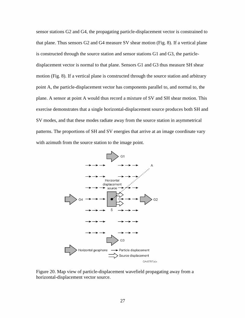
27
sensor stations G2 and G4, the propagating particle-displacement vector is constrained to
that plane. Thus sensors G2 and G4 measure SV shear motion (Fig. 8). If a vertical plane
is constructed through the source station and sensor stations G1 and G3, the particle-
displacement vector is normal to that plane. Sensors G1 and G3 thus measure SH shear
motion (Fig. 8). If a vertical plane is constructed through the source station and arbitrary
point A, the particle-displacement vector has components parallel to, and normal to, the
plane. A sensor at point A would thus record a mixture of SV and SH shear motion. This
exercise demonstrates that a single horizontal-displacement source produces both SH and
SV modes, and that these modes radiate away from the source station in asymmetrical
patterns. The proportions of SH and SV energies that arrive at an image coordinate vary
with azimuth from the source station to the image point.
Figure 20. Map view of particle-displacement wavefield propagating away from a horizontal-displacement vector source.

28
Numerous people have developed mathematical expressions that describe the
geometrical shape of P, SV, and SH radiation patterns produced by seismic sources in an
isotropic Earth. One of the respected references on this topic is White (1983). These
published analyses show that in map view, SH and SV radiation patterns produced by a
horizontal-displacement source have the appearance of that shown in Figure 21. Viewed
from directly above the horizontal-displacement source, SV and SH modes propagate
away from the source station as expanding circles. Because SV radiation from a
horizontal-displacement source is more energetic than SH radiation, SV radiation circles
are drawn larger than SH radiation circles. These circles indicate which parts of the
image space each mode affects and the magnitude of the mode illumination that reaches
each image coordinate. For example, a horizontal source-displacement vector oriented in
the Y direction (left side of figure) causes SV modes to radiate in the +Y and –Y
directions and SH modes to propagate in the +X and –X directions. A horizontal source-
displacement vector oriented in the X direction (right side of figure) causes SV modes to
radiate in the +X and –X directions and SH modes to propagate in the +Y and –Y
directions. If a line is drawn from the source station to intersect one of these radiation
circles, the distance to the intersection point indicates the magnitude of that particular
mode displacement in the azimuth direction of that line. The orientation of the particle-
displacement vector remains constant across the image space, as indicated in Figure 20,
but the magnitude of the SH and SV particle-displacement vectors vary with azimuth as
shown, respectively, by the SH and SV radiation circles in Figure 21.

29
Figure 21. Map view of SH and SV illumination patterns for orthogonal (X and Y) horizontal-displacement sources.
The shear-wave radiation associated with P-to-SV mode conversion is much
different from that produced by a horizontal-displacement source. Section and map views
of P-SV radiation patterns are provided as Figures 22 and 23, respectively. The section
view (Fig. 22) indicates an air gun operating in a water environment (a scalar source).
The converted-SV radiation patterns in this diagram apply equally well to land-based
operations where the energy source is a vertical vibrator or an explosive in a shot hole. In
both 3-C (land) and 4-C (marine) data acquisition, the SV radiation pattern associated
with the P-SV mode is produced in the subsurface at the P-to-SV conversion point, not at
the surface-based source station, as is the case for a horizontal-displacement source (Figs.
20 and 21). The map view in Figure 23 shows the downgoing-P mode propagating away
from the source station, with SV radiation patterns being produced at subsurface
interfaces at every point along the P wavefront. The dotted patterns indicate the
geometrical shape of the converted-SV radiation that is created at each subsurface P-to-

30
SV conversion point. A key point to note is that the orientation of the SV particle-
displacement vector is not in a fixed direction, as it is for a horizontal-displacement
source (Fig. 20), but varies with azimuth direction. The vector orientations shown in this
diagram are correct for an isotropic Earth where the total SV displacement is oriented in
the radial direction in which the P wave is propagating. In an anisotropic Earth, the SV
particle-displacement vector has both radial and transverse components.
Figure 22. Section view of P-SV radiation pattern.

31
Figure 23. Map view of P-SV illumination pattern.
Distinctions between 3-C and 9-C S-wave target illuminations are easier to
visualize if SV and SH radiation patterns associated with each type of data are viewed in
a side-by-side format as in Figure 24. These radiation patterns are descriptive of S-wave
propagation in an isotropic Earth, not an anisotropic Earth. Analysis of these illumination
behaviors leads to several conclusions.
1. A 3-C, scalar, P-wave source generates only an SV S-wave mode. A 9-C horizontal-displacement source creates both SH and SV modes.
2. An SH S-wave mode can be created by only an SH source, which by definition is a 9-C horizontal-displacement source.
3. A 9-C horizontal-displacement source creates SH and SV modes in the Earth volume immediately around its surface-station coordinates. A 3-C, scalar, P-wave source creates a converted-SV mode at subsurface coordinates remote from the source station.
4. In 9-C illumination, all SH and SV particle-displacement vectors throughout the propagation medium are oriented in the same direction as the horizontal source-displacement vector that created the modes. In 3-C illumination, orientation of the SV particle-displacement vector varies with azimuth direction away from the source station.

32
5. In 9-C target illumination, SH and SV particle-displacement vectors have a constant algebraic sign (polarity) throughout the propagation medium. In 3-C illumination, the particle-displacement vector of the converted-SV mode has an opposite algebraic sign (polarity) for any two propagation azimuths that differ by 180°.
6. In 9-C data acquisition, SH and SV modes illuminate the subsurface with a different intensity in each azimuth direction. In 3-C data acquisition, the converted-SV mode illuminates the subsurface with the same intensity in all azimuth directions.
Figure 24. Side-by-side comparison of 3-C and 9-C S-wave illumination patterns.
A final observation about 3-C and 9-C S-wave illumination is based on the
principles shown in Figure 25. This diagram illustrates distinctions between the
polarizations of SV modes in 3-C and 9-C seismic data, as seen in map view around a
source station. SH-mode polarization is not included in the illustration because a 3-C
source cannot create an SH mode. For each source, polarization behavior of the SV mode
is defined in terms of inline and crossline vector components in each of the four
quadrants that encircle the source position. When a P-wave source occupies the source

33
station, its downgoing-P wavefield illuminates all four quadrants with equal intensity
(Figs. 23 and 24). However, inline and crossline vector sensors measure a different
polarization for one or both of the horizontal, P-generated, SV displacements in each
quadrant, as illustrated in the left diagram. A single horizontal-displacement source will
not illuminate all four quadrants around a source station with equal intensity (Figs. 21
and 24). Two orthogonal horizontal-displacement sources must therefore occupy a source
station in 9-C data acquisition to create equivalent SV (and SH) illumination intensity
throughout the propagation medium. These orthogonal sources create the same SV
polarization in all quadrants (right diagram), which is significantly different from 3-C SV
polarization behavior.
Figure 25. Distinctions between 3-C (left) SV-mode polarization and 9-C (right) SV-mode polarization.
Elastic-Wavefield Seismic Stratigraphy
Multicomponent seismic data, whether 9-C or 3-C data, provide an important
new method for interpreting subsurface geology called elastic-wavefield seismic

34
stratigraphy. The fundamentals of this interpretation technique are discussed here
because several concepts documented in this report are critical to this emerging
technology. First, several key terms used in the methodology must be defined. A seismic
sequence a succession of relatively conformable seismic reflections bounded by
unconformities or their correlative conformities (Mitchum, 1977). The bounding surface
of a seismic sequence commonly occurs as a horizon that follows a trend of reflection
terminations. A seismic facies is defined as any seismic attribute that distinguishes one
succession of reflections from another succession of seismic reflections (Mitchum, 1977).
The science of seismic stratigraphy is based on recognizing seismic sequences and
seismic facies and then using the spatial geometries, arrangements, and distributions of
these sequences and facies to infer depositional environments and lithofacies patterns.
The concepts of seismic stratigraphy have dominated the science of seismic interpretation
ever since the fundamentals of seismic stratigraphy were made public by Exxon
researchers in the mid-1970’s (Payton, 1977).
Historical, or traditional, seismic stratigraphy is based on P-P seismic data.
Multicomponent seismic data now expand seismic stratigraphy into a new science
referred to as elastic-wavefield seismic stratigraphy. The basic premise of elastic-
wavefield seismic stratigraphy is that any mode of a multicomponent seismic wavefield
may provide unique seismic sequence information and/or unique seismic facies
information across some stratigraphic intervals that cannot be observed in the other
modes of the wavefield. Seismic stratigraphy analyses now do not need to be limited to
P-P data, as they have for decades.

35
The logic for the fundamental premise of elastic-wavefield seismic stratigraphy
is based on the principles discussed in the preceding sections. First, the particle-
displacement vectors of a multicomponent seismic wavefield test the properties of the
Earth in different directions (Fig. 1). As a result, the displacement vector of one mode
may detect seismic facies (Earth fabric) that are different from what other displacement
vectors detect and may be affected by stratal surfaces that are different from those that
affect the displacement vectors of other modes. Second, each wave mode illuminates a
target with a unique radiation pattern geometry, which may cause one mode to reveal a
target feature not seen with other modes. Third, all wave modes have distinct reflectivity
behaviors at an Earth interface, which sometimes causes one mode to emphasize a suite
of stratigraphic interfaces differently than do its companion modes.
If 9-C seismic data are used, Earth fabric can be measured using five
independent particle-displacement vectors (P-P, SH-SH, SV-SV, P-SV, SV-P). If 3-C
seismic data are used, Earth fabric can be tested using only two particle-displacement
vectors (P-P and P-SV). The increased number of independent fabric-sensing
displacement vectors associated with 9-C seismic data leads to the conclusion that more
rock, fluid, and general Earth-fabric information should be provided by 9-C seismic data
than by 3-C data. Similarly there is a greater likelihood that 9-C seismic data can image a
stratal surface that is not imaged by 3-C data, and that 9-C data can reveal a seismic
sequence or a seismic facies that is not revealed by 3-C data.

36
DATA-PROCESSING DIFFERENCES BETWEEN 9-C AND 3-C S-WAVE DATA
Software that transforms S-wave modes of 9-C seismic data into S images differs
in fundamental ways from software that produces S-wave images from 3-C data.
Common-midpoint (CMP) data-processing concepts, which have been used in oil and gas
applications for decades, can be used to produce S-wave images from 9-C data. A
different data-processing strategy called common-conversion-point (CCP) imaging is
required for constructing S-wave images from 3-C data. Key differences between these
two data-processing technologies (CMP and CCP) are described in this section.
Common Midpoint (CMP) Imaging
The basic requirement for CMP imaging is that the propagation velocity of the
reflected, upgoing wavefield be the same as the propagation velocity of the downgoing,
illuminating wavefield. In the P-P seismic imaging that the oil/gas industry has done for
approximately 50 years, downgoing and upgoing wavefields both travel at P-wave
velocity Vp. CMP software was developed originally to make only P-P images and has
been used for this restricted, seismic-mode imaging until recently. However, CMP
imaging can be applied in any situation in which the downgoing and upgoing wavefields
have equivalent propagation velocities. Thus, when 9-C data are acquired, SH-SH and
SV-SV images, in addition to P-P images, can be made with CMP software. Downgoing-
and upgoing-SH wavefields that travel with velocity VSH are segregated from the 9-C
wavefield and are used to make an SH-SH image. Downgoing- and upgoing-SV
wavefields that travel with velocity Vsv, which differs slightly from SH velocity VSH,, are
then extracted from the 9-C data and used to make an SV-SV image. Many versions of

37
CMP software are available throughout the seismic data-processing industry. Any of
these software packages can be used to process 9-C seismic data to create SH-SH and
SV-SV shear-wave images, in addition to the standard P-P compressional-wave image
that has been made for decades. The raypaths involved in CMP imaging are shown in
Figure 26. This diagram shows that in a flat-layered Earth, CMP reflection points
generated at different reflector depths stack vertically above each other at coordinate Xm,
the common midpoint, located halfway between the source station and the receiver
station. The image-point trend labeled CCP is discussed in the following section.
Figure 26. Distinction between 9-C CMP image points (vertical dash line) and 3-C CCP image points (curved dash line). Raypaths show the propagation paths involved in CMP imaging.
Common-Conversion-Point (CCP) Imaging
Common-midpoint (CMP) imaging concepts cannot be used when the
propagation velocity of the downgoing, illuminating wavefield differs from the
propagation velocity of the upgoing reflected wavefield. The most common situation
where this wave physics is encountered involves the P-SV mode, which is created when a

38
downgoing-P illumination wavefield converts to an upgoing-, reflected-SV wavefield via
P-to-SV mode conversion at a reflecting interface. As has been stressed in the preceding
sections, a P-SV mode is the only S-wave mode that can be extracted from 3-C seismic
data. The inverse mode, SV-P, which is created by a downgoing-, illuminating-SV
wavefield converting to an upgoing-, reflected-P wavefield via SV-to-P mode conversion
at a reflecting interface, is another situation where CMP data-processing concepts cannot
be used. An SV-P mode is available only with 9-C seismic data because an SV source is
required to produce the downgoing illumination wavefield.
For each of these converted-S modes (P-SV and SV-P), the image point does not
occur at common-midpoint coordinate Xm, as in CMP imaging. In 3-C (or 4-C) P-SV
imaging, the downgoing wavefield has a faster velocity (Vp) than the upgoing wavefield
(Vsv). As a consequence of Snell’s law, the image point does not occur at midpoint Xm
but at a coordinate that is closer to the receiver station than to the source station. This
image coordinate is called the common-conversion point (CCP). The raypaths involved in
CCP imaging of a P-SV mode are depicted in Figure 27. This diagram shows that in a
flat-layered Earth, CCP image points generated at different depths do not stack vertically
above each other, as do CMP image points, but move closer to the receiver station as
reflecting interfaces are imaged nearer the Earth surface.

39
Figure 27. Distinction between 3-C CCP image coordinates (curved dash line) and 9-C CMP image point coordinates (vertical dash line). Raypaths illustrate propagation paths involved in CCP imaging.
In 9-C SV-P imaging, the downgoing wavefield propagates at a velocity (Vsv)
slower than that of the upgoing wavefield (Vp). Now as a result of Snell’s law, the image
point occurs closer to the source station than to the receiver station. This image point is
still called a common-conversion point even though it is located at a subsurface
coordinate different from the CCP coordinate associated with 3-C P-SV imaging. The
raypath involved in 9-C CCP imaging of SV-P data is illustrated in Figure 28. Again, the
image points generated at different depths will not stack vertically above each other. In

40
contrast to 3-C P-SV imaging, SV-P image coordinates move closer to the source station,
not the receiver station, as reflecting interfaces approach the Earth’s surface.
Figure 28. Distinction between a 9-C SV-P CCP raypath (dash line) and a 3-C P-SV CCP raypath (solid line).
CMP and CCP Velocity Analyses
The stacking and migration velocities needed for 9-C (CMP) and 3-C (CCP) S-
wave imaging have to be determined by different analytical procedures. The fundamental
reason that an approach to velocity estimation has to be done for 9-C data that is different
from that for 3-C data can be explained by referring to the simple Earth model in Figure
29. In this model there is a change in rock facies along the imaging raypaths. P-wave
velocity Vp and SV velocity Vsv in Facies 1 are assumed to be different from the values
of Vp and Vsv in Facies 2.

41
Figure 29. Traveltimes for positive offsets are the same as traveltimes for negative offsets in 9-C CMP imaging because the lengths of the travel paths in Facies 1 and 2 are the same for both offset options.
The offset between source and receiver stations now has to be defined in terms of
the direction that the raypath takes to propagate from the source to the receiver. A
receiver offset to the right of the source will be defined arbitrarily as a positive offset;
receivers to the left of the source station will then be in the negative offset direction. In 9-
C CMP S-wave imaging (Fig. 29), the same raypath velocity and traveltime occur in both
negative and positive offset directions because the lengths of the travel paths in Facies 1
and in Facies 2 are the same when B is the source station and A is the receiver station
(negative offset) as they are when A is the source station and B is the receiver station
(positive offset). The same stacking and migration velocities are therefore calculated in
positive and negative offset directions when 9-C SH-SH and SV-SV data are processed.

42
A different conclusion is reached in 3-C P-SV CCP velocity analysis. The
raypaths involved in 3-C CCP imaging of the P-SV mode are shown in Figure 30. If A is
the source station and B is the receiver station (positive offset), the velocity of the
downgoing-P mode is controlled by Facies 1 and the upgoing-SV-mode velocity is
determined by Facies 2. The image coordinate is CCPA. When B is the source station and
A is the receiver station (negative offset), most of the P-wave velocity is controlled by
Facies 2, and all of the upgoing-SV raypath is in Facies 1. The image coordinate is now
CCPB. Assuming that velocities Vp and Vsv in Facies 1 differ from those of Vp and Vsv
in Facies 2, CCP stacking and migration velocities calculated for positive offsets and
negative offsets are not the same. That different velocity behaviors are observed in
opposite offset directions for 3-C P-SV imaging is a fundamental distinction between the
wave physics of 9-C and 3-C seismic data.
Figure 30. Traveltimes for positive offsets are not the same as traveltimes for negative offsets in 3-C CCP imaging because the lengths of the P and SV raypaths in Facies 1 and 2 change when the offset direction changes.

43
CMP and CCP Stacking
For a seismic image to be created, the image space between all source and
receiver pairs is segregated into small subvolumes called stacking bins. During data
processing, data traces are positioned across this image space by calculating the bin
locations where successive image points occur. In CMP (9-C) imaging in a flat-layered
Earth, image points occur at the midpoint between source and receiver regardless of the
depth of the reflecting interface (Fig. 26). A CMP trace is shifted in time (source-static
correction, receiver-static correction, other static corrections, and normal moveout
correction), and then the entire data trace is positioned vertically at the common midpoint
for the source-receiver pair that produced the trace. This type of imaging is indicated in
Figure 31 by the vertical data trace in stacking-bin column A located at the common
midpoint for the indicated source and receiver. That data trace is created at the indicated
source station and recorded at the labeled receiver station. In CMP image space, however,
the trace is positioned in stacking bin A at the midpoint between source and receiver
coordinates.

44
Figure 31. Comparison of 9-C CMP image trace (vertical in stacking bin A) and 3-C CCP image trace (curved across stacking bins 1 through 7).
Robust CMP stacking algorithms are widespread across the seismic industry,
and most commercial seismic data-processing shops have extensive experience in CMP
processing. Numerous seismic data-processing companies can therefore create good-
quality SH-SH and SV-SV images from 9-C data because CMP concepts that they
understand and have applied countless times are all that are required to create these S-
wave image options. The basic requirement is that a horizontal-displacement vector

45
source be positioned at the source station to create downgoing-SH and -SV illumination
modes. The raypath notation in Figure 31 indicates only downgoing- and upgoing-SV
modes because the objective is to distinguish between SV-SV and P-SV imaging.
The curved wiggle trace in Figure 31 shows where the data trace would be
distributed across the image space if a P-wave source occupied the source station, a 3-C
vector sensor occupied the receiver station, and the data were acquired according to 3-C
P-SV imaging constraints. In this case, the downgoing raypath is a P wave, and the
upgoing raypath is an SV mode. Now the static and normal-moveout time adjustments
made to the image trace affect data in several columns of stacking bins. Segments from
several CCP traces have to be patched together to create a vertically stacked trace in each
column of stacking bins. For example, three 3-C CCP-processed data traces that are
offset from each other by one bin dimension in seismic image space are shown in Figure
32. That part of trace A between points 1 and 2 has to be combined with the data window
extending from 2 to 3 in trace B and with the data window extending between points 3
and 4 in trace C to create a vertical wiggle trace extending from point 1 to point 4 in the
shaded column of stacking bins. 3-C CCP stacking is thus fundamentally different from
9-C CMP stacking. As a consequence of the more complex requirements of CCP
stacking, some seismic data-processing shops do not have software or experience needed
to do 3-C P-SV imaging. Even data-processing shops that have established themselves as
reputable CCP data imagers are still developing some critical software and improving
older algorithms.

46
Figure 32. Single vertical image trace in one stacking bin of CCP image space (shaded column) must be constructed by summing data from different time windows of all CCP traces that traverse the bin.
The parameter that controls the curvature of a CCP trace in CCP-image space is
the Vp/Vs velocity ratio in the propagation medium. A model that illustrates this fact for
small angles of incidence is presented as Figure 33. This simple, straight-raypath model
shows that a 3-C P-SV image coordinate is defined by offsets Xp and XSV from the
source and receiver stations and that these offsets are proportional to the Vp/Vs velocity

47
ratio in the propagation medium. The top equation listed in this illustration is Snell’s law
of reflection, the middle equation is a statement of the raypath geometry shown in the
model, and the bottom equation is valid when the incident angles are small enough that
sine is the same as tangent. For larger angles of incidence and reflection in a layered
Earth, the relationship between CCP image coordinates and the Vp/Vs velocity ratio is
more complicated than the simple equation in Figure 33. In real Earth media, a key
requirement of 3-C CCP processing is to create accurate Vp/Vs imaging functions across
seismic image space by first stacking P-SV data with a large number of Vp/Vs values and
then determining which Vp/Vs value produces optimal-quality stacked data at each image
coordinate. The concept is similar to the time-variant, space-variant, velocity-semblance
technology that is used to stack CMP data.
Figure 33. Simple, straight-raypath model showing that the velocity ratio Vp/Vs in the propagation medium controls the position of a 3-C P-SV image coordinate in seismic image space.
48
Although construction of 3-C P-SV images concentrates on determining accurate
values of Vp/Vs over the total image space, some data processors take shortcuts. The
most common shortcut is to do asymptotic binning. In asymptotic binning, the CCP
coordinate for the deep part of the image space, where the CCP image trace is almost
vertical (Figs. 31 and 32), is calculated, and then the entire data trace is assumed to be
vertically aligned at that coordinate. This approximation would cause all of the curved
trace in Figure 31 to be positioned in stacking bin 7, the asymptotic bin for that trace. The
deep part of the image would be correct, but the upper part would be incorrect, with the
imaging error increasing as the reflecting interface approaches the Earth’s surface. For
deep targets, asymptotic binning is acceptable. For shallow targets, it is not.
More advanced data-processing shops have abandoned asymptotic binning and
replaced that shortcut technique with procedures that calculate time-dependent and space-
dependent estimates of Vp/Vs over the total CCP image space. In so doing, however,
they still often take shortcuts, such as giving little attention to determining accurate
values of Vp/Vs in shallow data windows if there is no exploration interest in shallow
targets. This imaging philosophy is a practical procedure in the low-profit-margin
business of seismic data processing. There is no financial reward for work done to make
the shallowest part of a CCP image correct if no one is interested in shallow geology.

49
EXAMPLES OF 9-C AND 3-C SEISMIC DATA
Data from several multicomponent seismic surveys will be presented in this
section to illustrate selected concepts that distinguish 9-C S-wave data from 3-C S-wave
data. The ideal way to evaluate distinctions between 9-C and 3-C seismic data is to have
both 9-C and 3-C data acquired at the same location. However, two separate seismic
surveys are required to satisfy this same-location objective without biasing the analysis of
the data toward one or the other of the multicomponent technologies. Such bias will
likely occur if analysis is limited to a single seismic survey because 9-C CMP imaging
geometry differs from optimal 3-C CCP imaging geometry (Figs. 26, 27, 29, and 30).
Source-receiver geometries that result in high, uniform stacking fold of 9-C CMP data
rarely produce optimal image-fold conditions for 3-C CCP data. Similarly, most 3-C
seismic survey geometries are not optimal for 9-C CMP data acquisition. These
comments should not be construed to mean that a single seismic acquisition program
cannot be designed that will produce optimal-quality data for both 9-C and 3-C imaging.
We think that as multicomponent seismic technology gains acceptance, such surveys will
be done. The real-world situation for this study, however, was that no single survey using
a geometry that was optimal for both 9-C and 3-C data was available for our analysis. We
are not aware that such a survey exists anywhere.
We began this project with the rather naïve assumption that a 9C3D seismic
survey we called the Ashland Survey would be an ideal database for comparing 9-C and
3-C data. However, as we pursued the study we came to the conclusion that because the
Ashland Survey geometry was designed for CMP imaging, our findings would probably

50
be biased toward the advantages of SH-SH and SV-SV CMP modes, and the P-SV CCP
mode would not be judged on a fair basis. We thus decided to satisfy our research
objectives by explaining distinctions between 9-C and 3-C seismic data from theoretical
and data-processing points of view and then showing S-wave data acquired using surveys
in which the acquisition geometry was optimal for either 9-C or 3-C data, but not for
both. That decision dictated the content and format of this report.
Distinctions between SH-SH and SV-SV S-Wave Modes
The fundamental thesis of this investigation is that several S-wave modes can be
extracted from multicomponent seismic data and that each of these modes can provide
different geologic information about the Earth than can its companion modes. A concept
that has been stressed throughout this report is that the greatest differences between S-
wave modes occur when 3-C P-SV data are compared with 9-C SH-SH and SV-SV data.
However, we will depart from this thesis temporarily and start this section with an
example that illustrates the principle that even 9-C SH-SH and SV-SV S-wave data differ
in fundamental ways.
Data from the Ashland 9C3D seismic survey are displayed in Figure 34. These
data are prestack super gathers constructed to show distinctions between SV-SV and SH-
SH data in field-record format. The data-processing procedures used to transform the 9-C
data from field-coordinate data space (where SH-SH and SV-SV modes are mixed
together) to the radial-transverse data space used in this display (where SH-SH and SV-
SV modes are separated) were discussed by Simmons and Backus (1999) and will not be
repeated here.

51
Figure 34. 9-C SV-SV and SH-SH super gathers shown in field-record format (Simmons and Backus, 1999).
Two distinctions between SH-SH and SV-SV shear-wave modes can be illustrated
with this data example. First, the downgoing-SV mode converts to two upgoing modes,
SV and P, but the downgoing-SH mode converts to only one upgoing mode, SH. This
wave physics is demonstrated by the presence of both SV-SV and SV-P refraction events
in the SV-SV data but only SH-SH refraction events in the SH-SH data. These refraction
events are labeled on the data to ensure that there is no misunderstanding about what is
being viewed. We see in this SV-SV field record (left) the exact wavefield behavior
described by the SV dual-reflectivity equations in Figures 16, 17, and 19 and in the SH-
52
SH field record (right) the behavior indicated by the single-reflectivity equation in Figure
11. The fact that a downgoing-SH mode creates only a reflected-SH mode, but a
downgoing-SV mode creates both reflected SV and P is why the SH mode is sometimes
called a “pure” shear mode. Said another way, SH-SH field records contain only shear-
wave information, but SV-SV field records contain both S-wave and P-wave information
mixed together in a rather complicated way, as the SV reflectivity equations imply (Fig.
17). This distinction between SH-SH and SV-SV data is fundamental.
The events that curve across the data panels of Figure 34 between 2 and 3 seconds
are SV-SV reflection events (left panel) and SH-SH reflection events (right panel). It is
rare to see SV-P reflections in field-record formats. None is obvious in the left data panel
of the figure. However, SV-P reflections should contaminate the SV-SV reflections in
almost the same proportion as the SV-P refractions contaminate the SV-SV refractions.
The second distinction to note between the SV-SV and SH-SH data of Figure 34
is that there is a significant difference in SV and SH propagation velocities. This fact is
illustrated by marking the distances A and B that S-wave refraction events propagate
after 1.5 and 2 seconds of traveltime. As shown in the figure, distances A and B for the
SH-SH data are greater than distances A and B for the SV-SV data. SH velocity parallel
to bedding (the direction of refraction travel) is therefore greater than SV velocity.
To further demonstrate differences between SH and SV propagation velocities,
the super gathers in Figure 34 are processed to emphasize primary reflection events in the
time window between 2 and 2.5 seconds. These processed data are shown as Figure 35.
The normal-moveout corrections used to flatten reflection events in both the SH-SH and
SV-SV data were done using SH-derived stacking velocities. The SH-SH events are

53
flattened, as expected (right panel), but the SV-SV events are overcorrected (left panel).
This test is a compelling demonstration that SH stacking velocities are larger than SV
stacking velocities. Because stacking velocities are horizontal velocities, the test also
confirms that differences between SH and SV velocities exist at deep interfaces where
primary reflections originate, as well as at shallow refracting interfaces (Fig. 34).
Figure 35. 9-C SV-SV and SH-SH trace gathers after processing to emphasize primary reflections between 2 and 2.5 s. Reflection events in both modes are corrected to horizontal events with SH-derived velocities to demonstrate that SH and SV stacking velocities differ (Simmons and others, 1999).

54
Distinctions between SH and SV propagation velocities in a layered Earth were
published by Levin (1979, 1980) more than 2 decades ago. A part of Levin’s work is
repeated as Figure 36. This diagram shows that SH and SV velocities are equal when
modes travel vertically in a transverse isotropic (flat layered) Earth and when they
propagate away from their coincident point of origin at one particular takeoff angle
(where velocity curves cross). The velocities differ at all other propagation angles, with
the difference being greatest along the horizontal propagation axis. In the horizontal
direction, SH velocity is significantly greater than SV velocity, which is what the data in
Figures 34 and 35 confirm.
Figure 36. Wave mode velocities calculated for transverse isotropic (TI) media showing that 9-C SV and SH velocities differ in a flat-layered Earth (Levin, 1979; Levin, 1980). All wave modes propagate from a station positioned at the origin. The vertical axis represents downward, vertical propagation into the Earth. The horizontal axis represents propagation along the Earth’s surface.

55
In summary, two key concepts are described by these Ashland data: SV-SV data
are contaminated with SV-P data but SH-SH data are not, and SH velocity is different
from SV velocity. These two fundamental distinctions sometimes cause one of the 9-C S-
wave modes, either SH-SH or SV-SV, to react to geologic conditions in a way different
from that of the other mode. It is rarely apparent which mode, SH-SH or SV-SV, will
provide more valuable information about a particular target. The best policy is to acquire
data that allow both S-wave images to be created.
3-C Data Polarization
A key distinction between 9-C and 3-C S-wave data is that the polarization of the
P-SV mode provided by 3-C technology is fundamentally different from the polarization
of the SH-SH and SV-SV modes provided by 9-C technology. These distinctions are
emphasized in the discussions of the 3-C and 9-C radiation patterns illustrated in Figures
21 through 25. We use data from a good-quality 3C3D seismic survey here to
demonstrate that the preceding theoretical descriptions of P-SV polarization are correct.
For this demonstration, we select a source station at the center of the survey and
then show the 3-C response observed at each of the four corners of the survey grid. Data
acquired at receiver station 50 in the southeast corner of the survey and at receiver station
488 in the northwest corner are displayed in Figure 37. Because the azimuths from the
source station to these two receiver stations differ by approximately 180°, the
polarization of the P-SV data at these two receiver coordinates should differ by 180°.
Positions of the source station and receiver station and orientations of the orthogonal
inline and crossline vector sensors, RIL and RXL, are shown in the map views of the
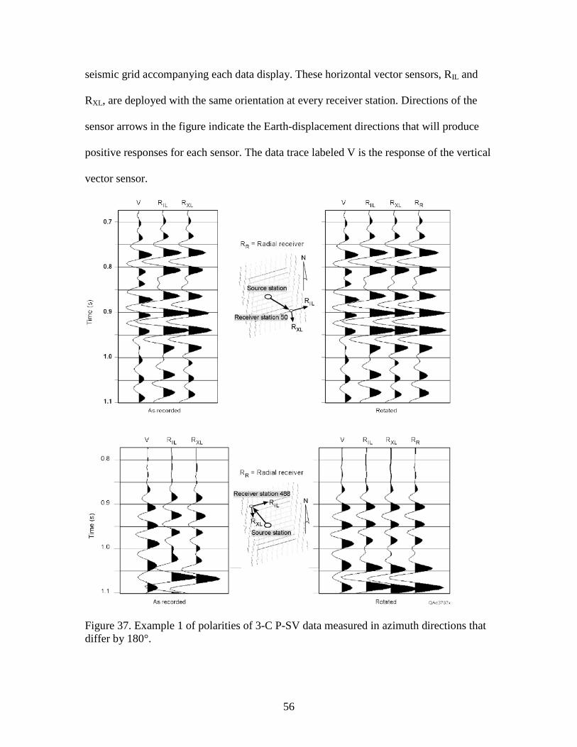
56
seismic grid accompanying each data display. These horizontal vector sensors, RIL and
RXL, are deployed with the same orientation at every receiver station. Directions of the
sensor arrows in the figure indicate the Earth-displacement directions that will produce
positive responses for each sensor. The data trace labeled V is the response of the vertical
vector sensor.
Figure 37. Example 1 of polarities of 3-C P-SV data measured in azimuth directions that differ by 180°.

57
Raw, unprocessed 3-C data are shown in the panels on the left. Comparing the top
and bottom panels shows that data recorded by orthogonal horizontal sensors at receiver
station 50 have the opposite algebraic sign to that of the data recorded at receiver station
488. Thus the P-SV data exhibit a 180° change in polarization for azimuth propagation
directions that differ by 180°, as Figure 25 indicates. The data panels on the right show
the P-SV data after processing steps have been taken to make the data appear to have
been created by a 9-C horizontal-displacement source. For a horizontal-displacement
source, there is no change in S-wave data polarity across the illuminated area (Fig. 25).
That constant-polarity condition exists for the P-SV data in the right panels, and P-SV
imaging can proceed only after this type of polarization correction has been made to all
of the 3C3D data.
For completeness, data acquired in the other two corners of the 3C3D survey are
shown in Figure 38. The principles illustrated here are the same as those that have been
discussed for Figure 37. First, P-SV data acquired at receiver station 537 in the northeast
corner have polarity opposite to the P-SV data acquired at receiver station 4 in the
southwest corner (left panels). Second, the data can be altered to represent constant-
polarization S-wave data similar to what would have been produced by a 9-C horizontal-
displacement source (right panels). The adjusted data in the right panels can now be used
for image construction.

58
Figure 38. Example 2 of polarities of 3-C P-SV data measured in azimuth directions that differ by 180°.
This P-SV data polarization discussion has been expanded to cover a larger
number of receiver stations by using an example from a second 3C3D seismic survey.
These data are shown in Figure 39. The data in this figure are a 2-D profile extracted
from the 3-D survey in which the receiver stations are inline with the source station. The
source station is between receiver stations 269 and 270 at the center of the profile. The

59
display documents response of the inline horizontal vector sensor along the profile. Data
in the top panel confirm that inline horizontal displacements measured to the right of the
source station (positive offset) have polarities that are opposite to the polarities of the
horizontal displacements measured to the left of the source station (negative offset). This
phenomenon is documented by comparing data polarities within data window A and by
comparing data polarities between data windows B and C. The bottom panel shows the
data after they have been polarity-adjusted to simulate 9-C horizontal-displacement
source data. The adjusted data in this bottom panel can now be processed to create a P-
SV image.

60
Figure 39. 2-D field record showing polarity behavior of the inline-horizontal component of P-SV data.

61
Making 3-C and 9-C Images Depth Equivalent
When multicomponent seismic data are processed to make stacked and migrated
images, S-wave images made from 9-C and 3-C data have different image-time axes
because the two-way traveltime of a P-SV mode for a particular target depth is different
from SH-SH and SV-SV traveltimes to and from that same depth coordinate. As a result,
9-C and 3-C S-wave modes position the reflection from a specific geologic interface at
different traveltime coordinates. The principal problem that confronts interpreters who
compare 9-C and 3-C S-wave data is the repeated dilemma of deciding which reflection
events in each image are depth equivalent across the seismic image space.
Probably the most rigorous method for depth registering 9-C and 3-C S-wave data
is to acquire and process multicomponent vertical seismic profile (VSP) data in a well
inside the image space spanned by a multicomponent seismic survey. Because VSP data
are acquired in the depth domain, each mode of a multicomponent VSP wavefield can be
converted directly into either a depth-based image or a traveltime image (Hardage, 2000).
An example of multicomponent VSP data being used to define depth-equivalent SH-SH
and SV-SV reflections was published by Hardage and others (2003). Depth registration
techniques for 9-C and 3-C seismic data are also being developed that are internally self-
consistent within the multicomponent data themselves and do not have to rely on external
calibration data such as a multicomponent VSP (Fomel and others, 2003).

62
CONCLUSIONS
Multicomponent seismic technology cannot be properly understood or applied
until all aspects of data generation, acquisition, processing, and interpretation are
structured on vector-based principles. When vector-based thinking is used, it becomes
more obvious why one S-wave mode may sense the Earth fabric differently than other S-
wave modes because the particle-displacement vector of each mode distorts the Earth in a
different direction relative to the bedding planes, laminae, fractures, and other physical
discontinuities that exist along the seismic propagation path. This concept that each S-
wave mode senses a different Earth fabric at a given subsurface coordinate is
fundamental to understanding why all S-wave modes should be used in prospect
evaluation rather than depending on only one S-wave mode to provide needed
information.
Nine-component (9-C) seismic data provide three S-wave modes (SH-SH, SV-
SV, and P-SV). Of these three modes, the SH-SH mode is the simplest in terms of its
reflectivity behavior and its lack of contamination from other modes. In contrast, three-
component (3-C) seismic data provide only one S-wave mode (P-SV). Each S-wave
mode (SH-SH, SV-SV, and P-SV) involves a different subsurface illumination pattern, a
different wavefield polarization, and a different reflectivity behavior. These distinctions
mean that one S-wave mode may provide a critical piece of geologic information about a
particular target that the other modes cannot. It is not possible to say that one S-wave
mode will be more valuable than the other modes in all types of geological imaging
problems. What can be said with confidence is that all information options are provided
by 9-C seismic data because all S-wave modes can be extracted from such data. In

63
situations where the SH-SH mode and/or the SV-SV mode (both being 9-C data) carries
more valuable information than that of the P-SV mode (3-C data), it is unwise to restrict
S-wave imaging to only 3-C technology.
In some cases, numerical modeling may indicate which S-wave mode will be the
more valuable option for evaluating a particular geologic target. However, numerical
modeling can sometimes be misleading. The safest course of action seems to be always to
acquire 9-C seismic data if at all possible. In those cases where budget considerations and
equipment constraints allow only 3-C data to be acquired, it is better to acquire 3-C data
than to be content with 1-C P-wave data.

64
REFERENCES
Aki, K., and Richards, P. G., 1980, Quantitative seismology-theory and methods: San
Francisco, W. H. Freeman and Company, 557 p. Fomel, S., Backus, M., DeAngelo, M., Murray, P., and Hardage, B., 2003,
Multicomponent seismic data registration for subsurface characterization in the shallow Gulf of Mexico: Offshore Technology Conference, Houston.
Hardage, B., 2000, Vertical seismic profiling principles: seismic exploration series, third
updated and revised edition: New York, Pergamon Press, v. 14, 552 p. Hardage, B., DeAngelo, M., and Murray, P., 2003 Defining P-Wave and S-wave stratal
surfaces with nine-component VSPs: The Leading Edge, v. 22, no. 8, p. 720–729. Levin, F. K., 1979, Seismic velocities in transversely isotropic media I: Geophysics, v.
44, p. 918–936. __________1980, Seismic velocities in transversely isotropic media, II: Geophysics, v.
45, p. 3–17. Mitchum, R. M., Jr., 1977, Seismic stratigraphy and global changes of sea level, part 11,
glossary of terms used in seismic stratigraphy, in Seismic stratigraphy-applications to hydrocarbon exploration: American Association of Petroleum Geologists, Memoir 26, p. 205–212.
Payton, C. E., 1977, Seismic stratigraphy-applications to hydrocarbon exploration:
American Association of Petroleum Geologists, Memoir 26, 516 pages. Simmons, J., Jr., Backus, M., Hardage, B., and Graebner, R., 1999, Case history: 3-D
shear-wave processing and interpretation in radial-transverse (SV-SH) coordinates (exp. abs), in Technical Program, 69th Annual International Meeting, Society of Exploration Geophysicists, v. 1, p. 792–795.
Simmons, J., Jr., and Backus, M., 1999, Radial-transverse (SV-SH) coordinates for 9-C
3-D seismic reflection data analysis (exp. abs), in Technical Program, 69th Annual International Meeting, Society of Exploration Geophysicists, v. 1, p. 728–731.
White, J. E., 1983, Underground sound—applications of seismic waves: New York,
Elsevier Science Publishers, 238 p.


![[sv] Validity date from LAND Marocko 00258 [SV] SECTION … · 2020. 5. 22. · 1 / 35 LAND [SV] SECTION Marocko Fiskeriprodukter [sv] Validity date from 10/08/2007 [sv] Date of publication](https://img.pdfslide.us/doc/110x75/5fbce723db71870cc10035f6/sv-validity-date-from-land-marocko-00258-sv-section-2020-5-22-1-35-land.jpg)